Download Santa Barbara Instrument Group ST-7E Operating instructions

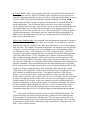
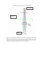
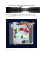
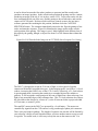
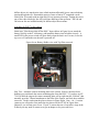
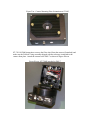
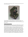
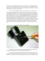
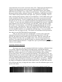
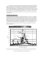
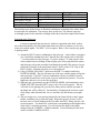
OPERATING INSTRUCTIONS
FOR THE
SANTA BARBARA INSTRUMENT GROUP
DEEP SPACE SPECTROGRAPH
(DSS-7)
AND
DSS-7 SPECTRAL CALIBRATION
PROGRAM (SCP)
Alan Holmes
4/27/2005
Overview: SBIG’s DSS-7 spectrograph will provide a powerful spectral measurement
capability to the amateur. Spectra of nebular, stellar, and galactic objects can now be
obtained with modest amateur telescopes as small as 4 inch aperture (but bigger is better).
While the SBIG Self Guided Spectrograph is optimized for high resolution stellar
measurements, the DSS-7 is more for spectral measurements of extended objects like
nebula and galaxies. The SGS has the ability to guide on a star while acquiring its
spectra, but the DSS-7 does not. This is because we have made the assumption that with
an extended object you can drift a little bit and still have the emitting region on the
entrance slit, at least more so than with a star. However, the DSS-7 is certainly capable
of stellar measurements. This manual describes connection of the spectrograph to an
SBIG camera, data collection at the telescope, and analysis of the resulting images to
obtain a spectrum of the source.
Spectroscopy Fundamentals: a spectrograph is an instrument that can produce a graph of
the intensity of light as a function of color, or wavelength. A spectrometer is a device
that measures only one selectable color, and a monochromator is a device that transmits
only one color. Wavelength is measured in Angstroms. An angstrom is one ten billionth
of a meter. You will also quite often see wavelengths written in nanometers, which is
one billionth of a meter. 6563 angstroms (A) is 656.3 nanometers (nm). The DSS-7
instrument is designed to separate and focus wavelengths from 4000 to 8000 angstroms
across the width of an ST-7 CCD. The human eye is sensitive from about 4500 (deep
blue) to 7000 (deep red) angstroms, with its peak sensitivity at 5550 angstroms. The
silicon CCD used in SBIGs cameras has a larger range of sensitivity than the eye. Most
stars put out a continuum of wavelengths with a number of absorption lines superimposed
upon the continuum. Most emission nebula like the Orion Nebula produce a spectrum
this is composed of a few bright emission lines, such as H-alpha (a hydrogen line at 6563
angstroms), H-beta (a hydrogen line at 4861 angstroms), and O-III (a triply ionized
oxygen line at 5007 angstroms). Galaxies have a spectrum that is an aggregate of many
stars, and have a similar spectrum to stars. Most galaxies only have a few obvious
features – the cores tend to show a sodium absorbtion line due to the older stars there.
Seyfert galaxies and other active galaxies show an excess of H-alpha, which is great since
it makes a red shift much easier to determine. Quasars, nova and supernova in general
exhibit strong 6563A emission. In the case of quasars it can be red shifted quite a bit,
hundreds of angstroms, so it may actually appear at a different wavelength. For a nova,
the line will only be shifted slightly since the star is in our own galaxy, but it may be
greatly broadened. The individual hydrogen atoms are moving very fast due to the
tremendous temperatures involved, producing Doppler broadening that smears out the
line.
Stars can be classified spectrally into the well know OBAFGKM groups. The
very hot stars have few features in their spectrum, perhaps only a few hydrogen lines.
The spectrum of Vega shown later illustrates this. The cool stars tend to be old, with
many metallic lines producing a very complex and structured spectrum. There are also
several types of peculiar stars, which show strong emission lines or other structure. The
DSS-7 can reveal these features.
Specifications: The DSS-7 will work with the SBIG ST-7/8/9/10/2000 cameras (with no
filter wheel attached), and the ST-402/1603/3200 line of cameras. It will not work with
the STL series of cameras since it cannot reach focus with them. It will also work with
ST-5C and ST-237 cameras, but with reduced spectral range due to the smaller CCD. It
might work with the ST-6 cameras, but we don’t offer an attachment that we know
works. The supplied software, SPECTRA, will work with images captured by the ST7/8/9/10/2000 line of cameras, and also with the ST-402/1603/3200 cameras, but not with
older cameras. The cameras that have larger CCDs than the ST-7 or ST-402 offer no
significant advantage in terms of spectral coverage – the design does not cover the larger
CCDs. The dispersion of the DSS-7 is 600 nanometers per mm, or about 5.4 angstroms
per pixel for the ST-7 (9 micron pixels). The resolution, which is less than the dispersion
due to blur and the finite slit width, is about 3 pixels, or 16 angstroms. The spectral range
captured by an ST-7 or ST-402 is about 4130 angstroms. The grating blaze is optimized
for 5000 angstroms.
Optical Design and Operation: the optical design of the DSS-7 is illustrated in Figure
One. Light enters the spectrograph through an entrance slit and is folded and then
collimated (made parallel) by the collimation lens. The light then impinges upon a
diffraction grating, which causes different colors to be reflected at different angles. You
can see a similar effect in the light reflected from a CD or DVD. The light diffracted
from the grating is then collected by a focusing lens, and imaged onto the CCD. Light of
a discrete wavelength through the slit will be imaged into a vertical line. If the light does
not fill the slit (such as is the case with a star) the discrete wavelength will produce a
starlike point on the CCD, with different wavelengths spread out along a line. This is
illustrated by the next few figures.
Figure One: Optical Layout of DSS-7 Spectrograph
CCD Location
Entrance Slit
Location
Grating
Figure Two shows the DSS-7 entrance slit. The narrow (50 micron) slit in the center is
flanked by a wider slit above (100 micron), and an even wider slit below (200 micron).
400 micron slits lie at the extreme top and bottom of the pattern. 50 microns is about
0.002 inch, smaller than a human hair, so the slits are quite narrow.
Figure Two: DSS-7 Entrance Slit
Figure Three shows the spectrum collected when this slit is illuminated by hydrogen light
– the two major wavelengths, 6563 and 4861 anstroms, produce two images of the slit
displaced horizontally. Figure Four shows a spectrum collected while examing P Cygni,
a peculiar star with permanent emission lines. The broadband radiation from the star
produces a horizontal line, while the emission lines show up as bright points, and the
airglow lines (some natural, some light pollution) show up as copies of the slit pattern.
For this image the airglow lines have been exaggerated to illustrate them better – P Cygni
is bright enough that exposures are short and airglow is not so prominent.
Figure Three: Hydrogen Spectra
Figure Four: Spectra of P Cygni and SkyGlow: Bright Points are 4861 and 6563
Angstroms
An obvious question at this point is “how does one put the star onto a 50 micron slit at
the focus of a telescope with an 2000 mm (80 inch) focal length”? Figure Five illustrates
the mechanics of the DSS-7.
Figure Five: DSS-7 Mechanical Configuration
The orientation shown here matches that of the optical schematic. The light enters from
the left. Both the slit and diffraction grating are motorized. The slit is motorized such
that it can be flipped in or out under computer control. The grating is motorized such that
it can be driven between the first order (produces a spectrum) and the zeroeth order
(produces an image) position. In the zeroeth order position the grating acts like a mirror,
producing an image of the slit, if it is in place, on the CCD. To put a star on the slit, the
user commands the slit out of the way, and the grating to the zeroeth order, and sets the
camera to FOCUS mode. He then uses his telescope controls to move the star into a
software generated box marking the slit position, and then clicks the CAPTURE
SPECTRUM button. The computer immediately inserts the slit, flips the grating to first
order, and starts the exposure. Figure Six illustrates the image quality in the zeroeth
order position of the grating. The image is good. Much light has been diffracted out of
this order by the grating, though, so objects are about 5 to 10X dimmer than without the
DSS-7.
Figure Six: Full Zeroeth Order Image on an ST-7XME (Nova Scorpius-2 in Center)
The DSS-7 is designed to accept an F/10 cone of light, a value typical of popular
commercial Schmidt-Cassegrain telescopes. In the imaging mode, it acts like a 2:1 focal
reducer, increasing the field of view of the CCD. It also is effectively a 2:1 focal reducer
in spectrograph mode, increasing the sensitivity to extended objects like nebulas or
galaxies. It will accept the center portion of the cone of light from a faster telescope, but
light is lost around the edges of the collimator lens. This 2:1 focal reduction also reduces
the slit width on the detector by a factor of 2, so the 50 micron slit has a projected width
of 25 microns, or around 3 pixels.
The small DC motors in the DSS-7 are powered by a 9 volt battery. The motors are
controlled by signals from the CCD camera’s relay port through a phone jack connector.
There is no provision for guiding. The length of exposure one can take will be limited by
your telescope’s ability to track unguided unless you have another camera set up to work
as a guider. For stellar work, it is not easy to keep the star on the narrowest slit. For
diffuse objects it is much easier since a little motion still usually leaves some nebulosity
passing through the slit. Reasonable spectra of stars as faint as 9th magnitude can be
achieved in 30 seconds with an eight inch (20 cm) aperture telescope. Putting the star in
one of the wider slits helps, but will yield some blurring of the spectrum. The 100 and
200 micron slits are included mainly for diffuse object observations.
Attaching the DSS-7 to the camera:
Initial step: Take the top plate off the DSS-7 shown below in Figure Seven, attach the
battery lead clip to the 9 volt battery, and install the battery into its holder securely. A
small LED in the power switch will glow dimly when the unit is on. For now, leave the
top cover off, and make sure the unit is powered off.
Figure Seven: Battery Holder view with Top Plate removed
Step Two – attach the camera mounting plate to the camera. Remove the three brass
thumbscrews and detach the camera mounting plate from the DSS-7. If you have an ST7/8/9/10/2000 the ring on the camera mounting plate will go right into the “D-block” that
normally provides T-thread attachment to the front of the camera, and lock down with the
setscrews. Do this, and orient the plate as shown in Figure Eight. Note – for –I version
cameras you will need to first attach the ring shown for the ST-402 in Figure Nine.
Otherwise you will not get to focus. If your –I camera has one of our taller t-rings in the
D-block you may need to contact us to get an adapter to let you reach focus.
Figure Eight: Camera Mounting Plate Orientation on ST-7XME
If you have a ST-402 camera, first screws the adapter into it as shown in Figure
Nine, and then attach the camera mounting plate oriented as shown in Figure Ten.
Figure Nine: Adapter Ring Mounted to ST-402
Figure Ten: Camera Mounting Plate Orientation on ST-402
ST-7/8/9/10/2000 instructions: remove the filter wheel from the camera (if attached) and
make sure the D-block/T-ring assembly shipped with the telescope is attached to the
camera front plate. Attach the camera to the DSS-7 as shown in Figure Eleven.
Figure Eleven: ST-7XME attached to DSS-7
Figure 12 shows a ST-402 attached to a DSS-7: Once again, note the orientation relative
to the ST-402 connectors.
Figure 12: ST-402 shown attached to DSS-7
The brass thumbscrews are used to attach the camera mounting plate to DSS-7 in both
cases so the camera can be slightly translated and rotated to bring it into perfect
alignment with the spectrum output by the DSS-7. For now, don’t worry about tightening
them too tightly.
Aligning the DSS-7 to the camera:
Leave the lid off the DSS-7 for now so you can see the mechanisms operate. A block of
pink foam may be under the metal spring strip that presses the motor shaft against the
grating mechanism arm. Remove it. We find that the motor shaft can leave a dent in the
O-ring material during long periods of storage, so we hold the pressure off with this
block. It would not be a bad idea to re-use it during long periods of inactivity. Next,
connect the phone cable provided from the ST-402 relay port to the DSS-7, or from the
ST-7XME relay port (using the RC-11 adapter) to the DSS-7. Power up the DSS-7 by
flipping the switch, and establish a link to the camera using CCDOPS. Using CCDOPS,
under the DSS-7 menu, select DSS MODE. A dialog box will appear. At the bottom,
make sure ENABLE DSS is not checked. We will first test the mechanisms. Exit that
dialog (hit OK), and select MOVE TELESCOPE under TRACK. Select XPLUS with a
time of 0.2 seconds, and hit OK. The grating assembly should rotate clockwise (CW) to
its limit. Next, select XMINUS and try it. The grating should rotate counterclockwise
(CCW). Do this a couple times to make sure it moves freely. Next, select YPLUS and
hit OK. The slit assembly should rotate into the entrance port. Select YMINUS and it
should rotate out. Do this a few times to verify it works properly. When done, install the
lid on the DSS-7 with the screws provided.
Now, go back to the DSS menu, and select DSS MODE. At the bottom of the
dialog box check ENABLE DSS-7. This will cause the relay outputs to be solely used
for controlling the DSS-7. If, at a later date, you need to use the relay port for guiding
you will need to uncheck this box. After checking the ENABLE box, select VIEW SLIT
with an exposure time of 1 second, room background light on the slit, and hit OK. The
DSS-7 slit will click into place, the grating will rotate CW, and a 1 second exposure will
be taken and displayed. It is probably out of focus. Use your normal FOCUS mode
under CAMERA to repetitively update this view. You should see an out-of-focus version
of the pattern in Figure Two. It is probably not centered, or square with the CCD edges,
but for now just concentrate on focusing it. Loosen the screws on the slider on the
bottom of the DSS-7 that carries the final focusing lens. The slider is shown in Figure
13.
Figure 13: Slider for focus adjustment
Slide this piece back and forth, intermittently tightening it down and observing
the image. When the image is as sharp as possible, tighten it down.
The next step is to center the slit image on the CCD array, and to line it up with
the sides of the CCD so there is minimal tilt of the spectrum. After loosening the brass
thumbscrews, manually center the slit image, and rotate the camera to align the slit image
vertical direction closely to the vertical axis of the CCD. Tighten down the thumbscrews,
and then loosen the setscrews on the camera attachment ring (for ST-402s and –I
cameras), or the D-block for ST-7 style cameras. Stop FOCUS mode, select GRAB
SPECTRA from the DSS-7 menu, with a ten second exposure. The grating will rotate to
the proper position, and the exposure collected. You should see wide stripes across the
CCD, which are the spectrum of the room light. Now, go back to CAMERA - FOCUS
mode, and start taking exposures with a few second duration. Use PLANET mode to get
a frame around the spectrum. Rotate the camera so the stripes are precisely horizontal.
Lock down the setscrews. Do not overtighten the setscrews or they put pits in the ring
that pull you off. You have now completed attachment and alignment of the spectrograph
to camera! You have one more adjustment before proceeding to the telescope. Using the
same computer you will use at the telescope, go to the DSS-7 menu, and select VIEW
SLIT with a 1 second exposure. You should get an image that shows the slit as before,
but well focused. Under the DSS-7 menu, select POSITION MARKER and a small
rectangle will appear on the screen. Drag the rectangle to the center of the slit image, and
size it to match the small slit, so it surrounds the small slit image. You can position it
around any of the two larger slits also. The software will remember the box position for
later when you use POSITION MODE at the telescope.
After you gain some experience with the DSS-7 you may want to repeat the
alignment of the spectra to better center the 400-800 nm region on the CCD, and
precisely line up the spectrum with the edges of the CCD. This may result in the slit
being a little bit off-center, and very slightly rotated. This will cause no problem in
operation. You might also note that the slit image in a spectrum might not be exactly
square with the dispersion direction. A slight error, up to 1 pixel horizontal per 40 pixels
vertical, is not a problem.
Capturing Calibration Spectrum:
The easiest way to become acquainted with the device and get a calibration frame
is to position a fluorescent shop light or desk lamp nearby, and point the entrance
aperture of the DSS-7 at a sheet of white paper illuminated by the lamp. Using GRAB
SPECTRA, with an exposure of 1 to 3 seconds, and you should see the horizontal
spectral stripes with a few vertical emission lines apparent. The brightest one is at 5461
Angstroms in the green, and the second brightest is at 4358 angstroms (deep blue). Figure
14 below illustrates what you should see with a ST-7XME and a DSS-7 while looking at
white paper illuminated by fluorescent tubes (5 second exposure in an office). Appendix
A contains a figure that will help you identify the spectral lines. Note that for a ST-402
the longest wavelengths are on the left, not the right as shown. The SPECTRA software
will work fine either way, as long as the same camera is used for calibration spectra as for
spectra of the object.
Figure 14: Spectrum of Room Light (lit by fluorescent) captured with ST-402
Once the spectrum has been captured, you need to crop it to inport it into SBIG’s
SPECTRA software. Using CCDOPS, select SPECTROSCOPY under the CROP menu
under the UTILITY menu. This will place a 765 pixel wide x 20 pixel tall box on the
screen, which you then place over the portion of the spectrum you wish to analyze. Next,
select CROP-CROP IMAGE under the UTILITY menu. You will get a strip as indicated
below in Figure 15. Save this with a different filename, such as with a –C on the end so
you don’t get it confused with the original file. You are now ready to analyze the strip
with SPECTRA.
Calibrating using Airglow lines:
If you are like most of us, you have significant light pollution in your area. Fortunately
that skyglow has a lot of well known spectral lines in it that can be used to self-calibrate
long exposure spectra. Figure 15 below illustrates a 20 minute exposure from a fairly
dark site near Atascadero, California, and my polluted backyard. The prominent lines are
labeled, and the longer wavelengths are on the right. When capturing skyglow lines (or
any diffuse object) you should use vertical binning of 4:1 or 8:1. Airglow data is very
easy to collect – you don’t need a lens at all, or tracking. Just point the entrance slit
aperture straight up!
Figure 15: Skyglow Spectra from Two Sites
8000
7000
High
Pressure
Sodium
6000
Counts
5000
Natural Lines
Light Pollution
4000
3000
Mercury
2000
1000
Dark Site
0
4000
4500
5000
5500
6000
6500
7000
7500
Wavelength in Angstroms
The prominent lines in the airglow you can use for calibration are tabulated in Table 1
Table 1: Prominent Skyglow and Airglow Lines.
Source
Street Lighting
Street Lighting
Atmospheric Oxygen
Street Lighting
Atmospheric Oxygen
Element
Mercury (Hg)
Mercury (Hg)
(O)
Sodium Vapor (Na)
(O)
Wavelength in Angstroms
4358.337
5460.753
5577.339
5686.5- aggregate (blend)
6300.304
The fact that some of these lines are blended combinations of multiple lines makes them
less desirable for calibration. The mercury lines are the best. The sodium vapor line
wavelength quoted is the centroid wavelength of the three lines that comprise this feature.
Operation at the Telescope:
I always recommend that one practice with new equipment in the back yard on
one of those beautifully clear full moon nights that seem to be so common, so as to not
waste time on dark nights. The DSS-7 is no exception. Below I list a step-by-step guide
to getting started.
1) Attach the DSS-7/camera combination to the telescope. – attach either a nosepiece
or a Visual Back attachment to the T-threads above the entrance slit on the DSS7. Securely attach it to the telescope. If you are using a 1.25 inch eyepiece tube
with a simple setscrew holding all that weight, put a safety strap between camera
and telescope to keep the assembly from hitting the ground if the setscrew lets go
(which they often do as the temperature drops). Power up the CCD. Flip on the
DSS-7 Switch. Align the telescope on a very bright star.
2) Using CCDOPS, select DSS-7, make sure the DSS-7 is enabled, and Select
POSITION MODE. The slit will rotate out of the way, and the grating will go the
mirror position. The DSS-7/camera combination will now work like a camera,
except that the small box exists on the screen to mark the slit position. Focus the
bright star, and move it over into the small box.
3) When the star is positioned, stop the POSITION MODE, and immediately select
GRAB SPECTRA from the DSS-7 menu, with a 10 second exposure. The slit
will rotate in, the grating will go to the first order position, and the spectrum of
the bright star will be collected. You should see a bright streak across the center
of the image when it downloads. Save it, and take any dark frames you might
need.
4) The next target to try is an emission nebula like the Orion Nebula or the Lagoon
nebula, something easy to find and bright. Repeat the process of steps 2 and 3,
but now select a vertical binning mode of 4 under the DSS-7 dialog, and use a 60
second exposure. You should see vertical lines corresponding to the brighter lines
in the object’s emission spectrum. You will need to take darks with similar
settings using the CAMERA – GRAB command. Vertical binning for this mode
can be set under CAMERA-SETUP.
Use of the SBIG DSS-7 Spectral Calibration Program (SCP) software:
SBIG’s WINDOWS 95/98/XP analysis software enables one to view the collected
spectra graphically, to calibrate the spectra, to print out graphical data, and to produce
text files with the raw data annotated with wavelength data. These text files can be
viewed with popular spreadsheet programs, which have more powerful graphing
capability. The calibration that is performed is a best fit to the grating equation using two
lines, and is good to about 0.1 pixel with adequate signal.
To install the software, install the CD disk with the DSS-7 SCP software into your PC,
and run the setup program. The setup utility will install the program and some sample
files.
If you run the program you will see the user screen shown in Figure 16. You should
begin by loading a calibration spectrum. Start by clicking on the LOAD CAL button, and
load the MERC.SBIG spectra. This spectrum was obtained by capturing a mercury
spectrum in low resolution mode. The SBIG Spectra program will only load files that are
less than 768 pixels wide and exactly 20 pixels tall, so the data was cropped to that shape.
Next, click LOAD DATA and load the NEON.SBIG data. Reselect the calibration data
by clicking the GRAPH CAL button.
Once the data is loaded you can click the ADJUST CONTRAST button to bring
up a dialog box that allows you to modify the background and range with which the
image is displayed. The analysis program uses the values that were saved with the
image, so if you get in the habit of adjusting the appearance before first saving the image
you will save time.
Using the long horizontal scroll bar underneath the graph, move the red tick
between the two spectral strips over to the line at 5460.7 nm (refer to Figure 16). You
can move the tick by either clicking on the ends of the scroll bar, or putting the mouse on
the slider between them, holding down the left button, and dragging it back and forth.
Center the spectral line between the two vertical lines on the graph. These two vertical
lines should be spaced to comfortably enclose 95% of the signal in the spectral line, but
not so far apart that neighboring spectral lines are included. The line spacing can be
changed using the SELECT WIDTH OF REGION control on the right side of the screen.
Click the down arrow, and choose the desired width from the options by clicking on it.
The line spacing should change on the graph. Five pixels wide is a good choice for the
example.
With the 5460.7 nm spectral line centered, click MARK LINE 1. The software
will then find the centroid of the spectral line to accurately determine its position. Next,
move the red tick mark to center the line at 4358.337 nm. Use the IDENTIFY
SPECTRAL LINE control to select 4358.337 nm. Click MARK LINE 2. The software
will complete the calibration and display the calculated focal length of the spherical
mirror in the spectrograph, and the spectral dispersion across the CCD in angstroms per
pixel. The dispersion is an approximation – the software uses the grating equation every
time it calculates a wavelength to minimize calculation errors. The focal length is about
50 mm, and the dispersion 600 angstroms per mm.
You are now ready to measure features in a spectrum. Click the GRAPH DATA
button to look at the neon data. Move the red tick over to a line, center the line, use the
CALCULATE LINE WAVELENGTH control to view the line’s wavelength (this control
uses the centroid of the data for accurate results). If the value is slightly off, select the
correct wavelength from the IDENTIFY SPECTRAL LINE box, and hit MARK LINE
ONE. Since the program has an active calibration it keeps the focal length parameter
from before, and adjusts the grating angle to compensate for the slightly different position
in the neon spectra. Now, move the red tick mark over to the other spectral lines visible
in the ring nebula image, center them, and click CALCULATE LINE WAVELENGTH
on the left side of the screen. The software will find the centroid of each line, and use the
grating equation to find the true wavelength.
Note that the border around the upper strip image is red. Click the GRAPH CAL
button to bring the calibration data back to the graph. Now if you center a line in the
graph, and click CALCULATE LINE WAVELENGTH you will see the center
wavelength of a feature in the calibration data. The calibration will still use the offset
calibration value from the neon data, though, so you need to recenter the 5460.7 nm line
in the calibration data, and click MARK LINE 1 again.
The CALCULATE LINE WAVELENGTH button works with absorption features
also. The software first looks to see if the center pixel is less than or greater than the
pixels marked by the lines to determine if it is an absorption feature or emission feature,
respectively, and then calculates the centroid appropriately.
The LINEAR GRAPH, LOG GRAPH, AUTOSCALED GRAPH, and PUSHED
GRAPH all affect the way the data is graphed in the graph box. For LINEAR GRAPH
the data is simply scaled from the minimum to the maximum of the data set. For LOG
GRAPH each factor of 10 in counts is scaled to one quarter of the graph box’s range. For
AUTOSCALED GRAPH, which is the most useful, the data is linearly scaled from the
maximum to the minimum of the portion of the spectrum within the graph box. For
PUSHED GRAPH the data is shown at maximum scale so features down in the noise can
be seen.
If you check the SMOOTHING ON box, the graph will be smoothed for display
purposes. If you click EXPAND SPECTRA, the gray scale display for both data and
calibration spectra will be displayed expanded vertically. Any slope in the lines is
removed, and faint features (real or not!) are more easily seen. If a calibration is active,
the displayed spectral data will be shown in color, matched to the visual perceived color.
Controls for cropping the calibration and data spectra are contained in the lower
right and left corners of the screen. If these controls are left at their default, 1 to 20, then
all 20 pixels in a column are summed and that data used for all calculations. You can
adjust the crop box to include only that portion of the spectra which contains stellar data.
This is a convenient feature. For example, collect some data on a star or nebula with the
calibration source on during the exposure. Crop the data to 765x20 and resave it. Load
the file into both the calibration and data spectra screens. Crop the CALIBRATION data
to just include the calibration lines above the object’s spectra, and crop the DATA spectra
to just include the object. Cropping is useful when the calibration data is captured at the
same time as the astronomical data, such as this. It can also improve the signal to noise
when very faint stars are being observed, when including all 20 pixels in a column when
only 4 have signal will increase the noise. Note – when moving the crop limits, the
display can take several seconds to update.
The FILTER AIRGLOW control can be used when the crop lines are moved off
the boundaries into the body of the strip. It subtracts off the airglow, based on what is
above or below the crop box. The USE MEDIAN control reduces noise by applying a
median filter to the data. The median filter works well since the noise is mostly “hot
pixel” in appearance.
To print out a graph of the spectrum for annotation or future reference, click the
PRINT GRAPH button. To write a text file containing the sum of the signal between the
crop lines, use the WRITE TEXT FILE button. The file created will be saved in the same
directory as the original file, with a .TXT extension. If a calibration is active the
wavelength data will be shown for each pixel. This text file can be opened with
Microsoft Excel or other spreadsheet programs. The data saved will be for the active
strip. IMPORTANT NOTE: if you wish to do quantitative measurement of the spectral
intensity data captured in a text file you need to subtract off an offset, which is
determined by looking at a region of the original CCD image away from the spectrum,
but representative of the background. Unfortunately a simple dark subtract is not enough
since there is usually a background glow in the atmosphere or due to grating stray light.
Determine this using the crosshairs within CCDOPS, and subtract 20 times the average
pixel value from your spectrum within EXCEL. Soemtimes a good background region is
captured in the spectral strip, but not always.
The SAVE STRIP FILE command creates a .ST7 file of the expanded spectra for
processing by CCDOPS with the intent of creating a publishable illustration. One can
also sample the screen image at any time by hitting the ALT-PRINT SCREEN keys on
the PC keyboard, which copies a bitmap of the screen into the clipboard. One can then
PASTE the image into PAINT, or other programs, where it can be manipulated.
If you need to calibrate using spectral lines that are not part of the list, please use
the MANUAL ENTRY option at the bottom of the spectral line list. Then enter the
wavelength of the calibration line in Angstroms in the dialog box that pops up.
Version 1.0 of the DSS-7 SCP software should read ST-7/8/9/10/2000 images up
to 768 pixels wide and 20 pixels tall. Users with ST-8s, ST-10s and ST-2000s should
crop the images to 765 x 20 pixels.
Collecting Astronomical Spectra:
To gain experience with the device and the software, we recommend you start out
measuring some bright stars and bright nebulas. With the stars you will find that red
stars, such as Betelgeuse, Arcturus, and Antares have copious spectral lines. These lines
will not be fully resolved. Many easily identified lines are blurred together , such as the
magnesium triplet at 5167.328, 5172.698, and 5183.619 A, and the sodium doublet at
5889.973 and 5895.940 A, but the aggregate lines are detected. Bright blue stars, such as
Sirius and Vega have much less distinct lines, but have broad absorption features around
H-alpha (6562.808 A), H-beta (4861.342 A) and H-gamma (4340.475 A). Note that the
breadth of these features is different between stars of different temperatures. Stars with
hotter coronas have broader features (Doppler broadening).
With nebular objects, you should have no problem finding H-alpha, H-beta, and
atomic oxygen (5007 A) lines. Faint diffuse objects are easy if the spectrum is composed
of emission lines.
The red shift of a spectral line in angstroms is well approximated by the following
equation:
Red shift = Z = (wavelength observed-wavelength actual)/(wavelength actual)
Z = velocity/C, where C = 300000 km per second (for non-relativistic speeds)
Objects moving away from you are shifted to the red. Our position in the spiral arm of
the Milky Way results in a 215 km per second imposed on objects outside the galaxy,
depending on their direction relative to the galactic equator (which is quite tilted relative
to the celestial equator). Velocities of remote galaxies are sometimes given relative to
the center of the Milky Way, so use reference publications carefully.
When you are comfortable with the unit, you can attempt measuring galactic red
shifts. Galaxies are hard since they are faint, extended, and mostly have continuum
spectra. Capture some spectra with long exposures, such as 10 to 20 minutes, with
multiple exposures. One usually does not need a calibration lamp on during the exposure
since light pollution and natural airglow lines will be recorded, but at a low level. It is
much easier to measure red shifts for Seyfert galaxies, which have an excess of H-alpha
and show emission lines, than other galaxies. Even the knots of H-alpha in galactic arms
may be easier than the core. Take a conventional CCD image with an H-alpha filter or
red filter to reveal the H-alpha regions, which can then be positioned on the slit. They
may be difficult to see, and may require that you estimate where they are from the galaxy
core and nearby stars, and put the desired part of the sky on the slit. One trick is to rotate
the spectrograph so that the slit runs through both the core and the H-alpha region, so you
can improve your chances of hitting it. While rotating the spectrograph-camera
combination is not that easy, neither are hour-long exposures. If you are capturing
spectra of galaxies with little H-alpha, look for the blurred sodium doublet absorption
feature to detect red shifts, and compare it with spectra of M0 stars. The older red stars
that comprise most galaxy cores show the sodium feature. Higher resolution would not
produce a sharper view of the doublet since the random motion of the stars within the
galaxy blur the spectral features to several angstroms width anyway.
M82 is a bright galaxy with a small red shift but copious H-alpha and very high
velocities in its core. It is a good initial target to see galactic spectral lines.
Quasars can be detected. Their spectrum approximates a galaxy with
superimposed emission lines. Fortunately their energy in spectral lines is great so, while
they are faint, their red shift is more easily measured than galaxies. Novae and
Supernovae are also fairly easy. Supernova down to about 14th magnitude can be
captured with an 8 inch (20 cm) aperture telescope.
Calibration Lamps – I’ve used the Edmund H71559 Power Supply ($175) and some
spectral tubes (Mercury = H60908, and Neon = H60910, each around $30) as calibration
sources – they work well and the price is reasonable. They also have hydrogen tubes
available. You can do quite well with fluorescent tubes and skyglow lines, though, so
don’t feel you have to buy these lamps. Also, do not use these high voltage tubes while
standing in wet grass – you can get zapped.
Important Safety Warning: if you use calibration lamps such as a Mercury PenRay that
emits short wave UV (at around 2537 Angstroms, or 253.7 nM), be very careful with
corneal and skin sunburn from the lamps. The little mercury PenRays (such as an
Edmund H40759) with quartz envelopes, held one foot from your face for five minutes,
will put you in the hospital. They do not appear that bright, but the UV emission is
tremendous. Even one minute will give you a sunburn and scratchy, dry feeling eyes. I
have personally suffered the effects of exposure to these sources twice, and have had two
coworkers (separate incidents) requiring bandaging of their eyes after exposure. The
SBIG spectrometer does not detect these short UV wavelengths, so long wave mercury
sources are adequate.
Literature:
The field of amateur spectroscopy is quite new. Only now is equipment commercially
available to make measurements of stellar spectra, radial velocity, and emission nebula.
As a result there is a shortage of publications that help the amateur interpret the spectra
obtained, and plan interesting observing programs. The popular magazines are beginning
to fill this shortage, working in conjunction with the advanced amateurs using our
equipment. As the discipline matures we will strive to build the capability into our
equipment that is needed, for presently we too have limited knowledge of what the
amateur desires.
Some interesting web sites with lots of spectral data are Maurice Gavin’s
(www.astroman.fsnet.co.uk), and Christian Buel’s (www.astrosurf.org/buil/). You will
find that both highly recommend slitless spectrographs. I have not chosen that design
here because of the problem of confusing zero order background stars with spectral
features, and the impossiblity of doing good measurements on extended sources such as
nebula and galaxies. Dale Mais also has a lot of good information at his web site at
www.mais-ccd-spectroscopy.com.
Appendix B: Control Port Connections and Conventions
The SBIG relay port (AO/CFW/Scope Port) controls the motors in the DSS-7. The “X”
relays control the grating and the “Y” relays the slit. Commanding a relay for 0.2
seconds is sufficient to change the slit or grating position. The controls are as follows:
+X relay: rotates grating to clockwise limit
-X relay: rotates grating to counterclockwise limit
+Y relay: rotates slit in (visible through entrance port)
-Y relay: rotates slit out of way
Almost 0.5 ampere is drawn from the battery during actuation, so if you write your own
control software keep the relay times short to avoid exhaustng the battery.