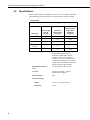
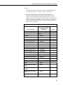
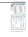
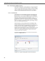
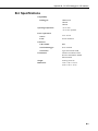
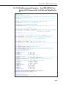
1
CDM-VW300 Series
Dynamic Vibrating-Wire
Analyzers
Revision: 10/13
C o p y r i g h t © 2 0 1 3
C a m p b e l l S c i e n t i f i c , I n c .
Warranty
“PRODUCTS MANUFACTURED BY CAMPBELL SCIENTIFIC, INC. are
warranted by Campbell Scientific, Inc. (“Campbell”) to be free from defects in
materials and workmanship under normal use and service for twelve (12)
months from date of shipment unless otherwise specified in the corresponding
Campbell pricelist or product manual. Products not manufactured, but that are
re-sold by Campbell, are warranted only to the limits extended by the original
manufacturer. Batteries, fine-wire thermocouples, desiccant, and other
consumables have no warranty. Campbell’s obligation under this warranty is
limited to repairing or replacing (at Campbell’s option) defective products,
which shall be the sole and exclusive remedy under this warranty. The
customer shall assume all costs of removing, reinstalling, and shipping
defective products to Campbell. Campbell will return such products by surface
carrier prepaid within the continental United States of America. To all other
locations, Campbell will return such products best way CIP (Port of Entry)
INCOTERM® 2010, prepaid. This warranty shall not apply to any products
which have been subjected to modification, misuse, neglect, improper service,
accidents of nature, or shipping damage. This warranty is in lieu of all other
warranties, expressed or implied. The warranty for installation services
performed by Campbell such as programming to customer specifications,
electrical connections to products manufactured by Campbell, and product
specific training, is part of Campbell’s product warranty. CAMPBELL
EXPRESSLY DISCLAIMS AND EXCLUDES ANY IMPLIED
WARRANTIES OF MERCHANTABILITY OR FITNESS FOR A
PARTICULAR PURPOSE. Campbell is not liable for any special, indirect,
incidental, and/or consequential damages.”
Assistance
Products may not be returned without prior authorization. The following
contact information is for US and international customers residing in countries
served by Campbell Scientific, Inc. directly. Affiliate companies handle
repairs for customers within their territories. Please visit
www.campbellsci.com to determine which Campbell Scientific company serves
your country.
To obtain a Returned Materials Authorization (RMA), contact CAMPBELL
SCIENTIFIC, INC., phone (435) 227-9000. After an application engineer
determines the nature of the problem, an RMA number will be issued. Please
write this number clearly on the outside of the shipping container. Campbell
Scientific’s shipping address is:
CAMPBELL SCIENTIFIC, INC.
RMA#_____
815 West 1800 North
Logan, Utah 84321-1784
For all returns, the customer must fill out a “Statement of Product Cleanliness
and Decontamination” form and comply with the requirements specified in it.
The form is available from our web site at www.campbellsci.com/repair. A
completed form must be either emailed to [email protected] or faxed to
(435) 227-9106. Campbell Scientific is unable to process any returns until we
receive this form. If the form is not received within three days of product
receipt or is incomplete, the product will be returned to the customer at the
customer’s expense. Campbell Scientific reserves the right to refuse service on
products that were exposed to contaminants that may cause health or safety
concerns for our employees.
Table of Contents
PDF viewers: These page numbers refer to the printed version of this document. Use the
PDF reader bookmarks tab for links to specific sections.
1. Introduction .................................................................1
2. Cautionary Statements...............................................2
3. Initial Inspection .........................................................2
4. Overview ......................................................................3
4.1
4.2
4.3
4.4
4.5
4.6
Channel Allocations .............................................................................3
Measurement Rates ..............................................................................4
Integrated Thermistor Measurement ....................................................4
Laboratory Mode..................................................................................5
Field Mode ...........................................................................................5
Data Uses .............................................................................................6
4.6.1 Static Measurements .....................................................................6
4.6.2 Dynamic Measurements................................................................6
4.6.3 Thermistor Measurements.............................................................6
4.6.4 Rainflow Histograms ....................................................................7
4.6.5 System Diagnostics .......................................................................7
5. Specifications .............................................................7
5.1
5.2
Features ................................................................................................7
Specifications .......................................................................................8
6. Installation .................................................................10
6.1
Laboratory-Mode Installation ............................................................11
6.1.1 Laboratory-Mode Installation Equipment...................................11
6.1.2 Laboratory-Mode Installation Procedure ....................................12
6.2
Field-Mode Installation ......................................................................18
6.2.1 Field-Mode Installation Equipment ............................................18
6.2.2 Field-Mode Installation Procedure..............................................18
7. System Operation .....................................................26
7.1
PC Based Tools ..................................................................................26
7.1.1 Software and Driver Installation .................................................26
7.1.2 Using DVWTool.........................................................................27
7.1.2.1 Ensure Connection is Active ............................................27
7.1.2.2 DVWTool Settings Editor ................................................28
7.1.2.3 Button and Field Descriptions..........................................28
7.1.3 Using DevConfig ........................................................................29
7.1.3.1 Ensure Connection is Active ............................................29
7.1.3.2 DevConfig Settings Editor ...............................................30
i
Table of Contents
7.2
7.3
7.4
Using the Datalogger......................................................................... 30
Using the SC-CPI Interface ............................................................... 31
Using Power Supplies........................................................................ 31
7.4.1 CDM-VW300 Series Analyzer Power ....................................... 31
7.4.2 Data-Acquisition System Power................................................. 32
7.5
Configuring the CDM-VW300 Analyzer .......................................... 32
7.5.1 Device Name .............................................................................. 34
7.5.2 CPI Bus Speed............................................................................ 34
7.5.3 Operating System Version.......................................................... 35
7.5.4 Operating System Date............................................................... 35
7.5.5 Analyzer Serial Number............................................................. 35
7.5.6 Display Rate ............................................................................... 35
7.5.7 Dynamic Sample Rate ................................................................ 35
7.5.8 Device Type ............................................................................... 35
7.5.9 CPI Bus Address ........................................................................ 35
7.5.10 System Options .......................................................................... 35
7.5.11 Channels Enabled....................................................................... 36
7.5.12 Desired Resonant Amplitude...................................................... 36
7.5.13 Minimum- and Maximum Cut-Off Frequencies ........................ 36
7.5.14 Frequency-Output Format .......................................................... 36
7.5.15 Multipliers and Offsets............................................................... 36
7.5.16 Steinhart-Hart Coefficients......................................................... 36
7.5.17 Rainflow-Histogram Output Configurations .............................. 36
7.6
Sensor Selection ................................................................................ 37
7.6.1 Frequency Considerations .......................................................... 37
7.6.2 Noise Performance ..................................................................... 37
7.7
System Connections .......................................................................... 37
7.7.1 CDM-VW300 to PC Connection ............................................... 38
7.7.2 CDM-VW300 to Sensor Connection.......................................... 38
7.7.3 CDM-VW300 to SC-CPI Connection ........................................ 40
7.7.4 CDM-VW300 to Power Connection .......................................... 42
7.7.5 Earth Ground Connections ......................................................... 44
7.7.6 Communication Connections ..................................................... 44
7.7.6.1 SC-CPI to CPI Bus Connection....................................... 44
7.7.6.2 Datalogger to SC-CPI Connection................................... 44
7.7.7 Maximum Number of Analyzers on a Datalogger ..................... 45
7.8
Operating System .............................................................................. 46
7.9
Power-Up Sequence .......................................................................... 46
7.10 CRBasic Programming...................................................................... 47
7.10.1 Writing Programs ....................................................................... 47
7.10.2 Sending Programs to the Datalogger.......................................... 48
7.11 System Adjustments .......................................................................... 49
7.11.1 Frequency Range........................................................................ 49
7.12 System Validation ............................................................................. 49
7.12.1 Sensor Validation ....................................................................... 49
7.12.2 Monitoring System Performance................................................ 49
7.12.2.1 Monitoring with DVWTool Software.............................. 52
7.12.2.1.1 Fault Detection...................................................... 52
8. Troubleshooting........................................................53
8.1
8.2
8.3
8.4
8.5
Connections ....................................................................................... 53
Power................................................................................................. 53
Isolating Components........................................................................ 53
Filtering Harmonics........................................................................... 54
Diagnostic Outputs ............................................................................ 54
ii
Table of Contents
8.5.1 Diagnostic Codes (Dynamic) ......................................................54
8.5.1.1 Description of Diagnostic Parameters ..............................55
8.5.1.2 Calculating Low- and High-Frequency Boundaries .........56
8.5.1.3 Using Diagnostic Parameters ...........................................57
8.5.1.4 Decoding the Diagnostic Code.........................................57
8.5.1.4.1 Excitation Strength ................................................57
8.5.1.4.2 Low-Amplitude Warning Flag ..............................57
8.5.1.4.3 High-Amplitude Warning Flag..............................58
8.5.1.4.4 Low-Frequency Warning Flag...............................58
8.5.1.4.5 High-Frequency Warning Flag ..............................58
8.5.1.4.6 Interpreting the Diagnostic Code...........................58
8.5.2 Standard Deviation of Dynamic Output......................................59
8.6
Factory Default Reset.........................................................................59
9. Glossary ....................................................................60
10. References and Attributions....................................60
Appendices
A. Measurement Theory.............................................. A-1
A.1
Dynamic Vibrating-Wire Measurements ........................................ A-1
A.1.1 Dynamic and Static Frequencies .............................................. A-2
B. SC-CPI Datalogger to CPI Interface....................... B-1
B.1
B.2
B.3
B.4
Introduction......................................................................................B-1
Quickstart .........................................................................................B-1
Overview..........................................................................................B-1
Specifications ...................................................................................B-3
C. CDM Devices and CPI Bus ..................................... C-1
C.1
CDM Interconnection and Datalogger Connection ..........................C-1
C.1.1 Power ........................................................................................C-1
C.1.2 Interconnect Cable ....................................................................C-1
C.1.3 Speed as a Function of Distance ...............................................C-2
C.1.4 CPI Grounding ..........................................................................C-3
C.1.6 Addressing ................................................................................C-3
C.2 Distributed Architecture...................................................................C-3
D. Digits Conversion ................................................... D-1
D.1
Example: Frequency to Digits to Displacement .............................. D-1
E. Calculating Measurement Error............................. E-1
E.1
E.2
E.3
E.4
E.5
Example Error Calculation: Geokon Strain Gage ............................E-1
Example Error Calculation: DGSI Embedment Strain Gage ...........E-2
Example Error Calculation: DGSI Spot-Welded Strain Gage..........E-2
Example Error Calculation: Geokon 4420 Crack Meter ..................E-2
Example Error Calculation: DGSI Piezometer 52611099................E-3
iii
Table of Contents
F. Thermistor Information........................................... F-1
F.1
Converting Resistance to Temperature.............................................F-1
F.1.1 Resistance Conversion Example – Geokon Sensor ...................F-1
F.2
Accuracy and Resolution..................................................................F-1
G. CRBasic Program Library ......................................G-1
G.1
Dynamic Measurements .................................................................. G-1
G.1.1 20 Hz Measurement Example — One CDM-VW300, Two
Channels ............................................................................... G-1
G.1.2 20 Hz Measurement Example — One CDM-VW305, Eight
Channels ............................................................................... G-2
G.1.3 20 Hz Measurement Example — Three CDM-VW305s, 24
Channels ............................................................................... G-4
G.1.4 20 Hz Measurement Example — Six CDM-VW305s, 48
Channels ............................................................................... G-5
G.1.5 50 Hz Measurement Example — One CDM-VW300, Two
Channels ............................................................................... G-8
G.1.6 50 Hz Measurement Example — One CDM-VW305, Eight
Channels ............................................................................... G-9
G.1.7 50 Hz Measurement Example — Three CDM-VW305s, 24
Channels ............................................................................. G-11
G.1.8 50 Hz Measurement Example — One CDM-VW300, Two
Channels, Rainflow Histogram........................................... G-12
G.1.9 50 Hz Measurement Example — One CDM-VW305, Eight
Channels, Rainflow Histogram........................................... G-14
G.1.10 50 Hz Diagnostic Example — One CDM-VW300, Two
Geokon 4000 Sensors with FieldCal()................................ G-15
G.1.11 50 Hz Measurement Example — One CDM-VW300, Two
Geokon 4000 Sensors with FieldCal()................................ G-17
G.1.12 50 Hz Measurement Example — One CDM-VW300, Two
Geokon 4000 Sensors with FieldCal() and CardOut() to
CF ....................................................................................... G-19
G.1.13 50 Hz Measurement Example — One CDM-VW300, Two
Geokon 4000 Sensors with FieldCal() and TableFile() to
CF ....................................................................................... G-21
G.1.14 100 Hz Measurement Example — One CDM-VW300, Two
Channels ............................................................................. G-23
G.1.15 100 Hz Measurement Example — One CDM-VW305,
Eight Channels.................................................................... G-24
G.2 Static Measurements...................................................................... G-25
G.2.1 1 Hz Measurement Example — One CDM-VW300, Two
Channels ............................................................................. G-25
G.2.2 1 Hz Measurement Example — One CDM-VW305, Eight
Channels ............................................................................. G-26
Figures
4-1.
4-2.
4-3.
4-4.
4-5.
4-6.
Two-channel CDM-VW300 wiring panel ........................................... 3
Eight-channel CDM-VW305 wiring panel.......................................... 4
Measurement speeds of the AVW200 and CDM-VW300 analyzers .. 4
Single-coil vibrating-wire sensor including coil and thermistor
outputs.............................................................................................. 5
Laboratory-mode measurement system diagram................................. 5
Field-mode data-acquisition system diagram ...................................... 6
iv
Table of Contents
6-1.
6-2.
6-3.
6-4.
6-5.
6-6.
6-7.
6-8.
6-9.
6-10.
6-11.
6-12.
6-13.
7-1.
7-2.
7-3.
7-4.
7-5.
7-6.
7-7.
7-8.
7-9.
7-10.
7-11.
7-12.
7-13.
7-14.
7-15.
7-16.
7-17.
7-18.
A-1.
B-1.
C-1.
C-2.
D-1.
F-1.
F-2.
F-3.
F-4.
Laboratory-mode measurement system..............................................11
12 Vdc power connection on the CDM-VW300................................12
USB receptacle on CDM-VW300 and Type-Micro-B connector
of USB cable...................................................................................13
Sensor connection on a CDM-VW305...............................................16
Three-wire vibrating-wire sensor connections ...................................16
Five-wire vibrating-wire sensor connections .....................................16
Field data-acquisition system .............................................................18
CPI communications links .................................................................21
Datalogger to SC-CPI connection ......................................................21
Connecting the CPI ports of the SC-CPI and CDM-VW300 .............22
Install CPI bus terminator ..................................................................22
Power connection ...............................................................................23
Earth ground connections...................................................................24
DVWTool Settings Editor and Data Display .....................................28
DevConfig Settings Editor .................................................................30
12 Vdc power transformer for laboratory-mode installation..............31
USB port on the CDM-VW300..........................................................38
Three-wire vibrating-wire sensor leads..............................................38
Three-wire vibrating-wire sensor connection.....................................39
Five-wire, vibrating-wire sensors leads..............................................39
Five-wire vibrating-wire sensor connection.......................................40
SC-CPI and CDM-VW300 CPI ports with RJ45 cable marked
with yellow tape..............................................................................41
CPI terminator installed .....................................................................41
Multiple analyzers on a CPI bus ........................................................42
Installing 12 Vdc transformer on the CDM-VW300..........................43
Daisy-chaining 12 Vdc power input on the CDM-VW300................43
Earth ground connections...................................................................44
CR3000 and SC-CPI connections ......................................................45
LoggerNet connect screens showing frequencies from
CDM-VW300 .................................................................................50
RTDAQ screens showing frequencies in Public table.......................51
Dynamic Vibrating-Wire Tool Box Fault Indicators .........................52
Timing of dynamic vibrating-wire measurements .......................... A-2
Connection to the SC-CPI in DevConfig .........................................B-2
CPI pin assignments.........................................................................C-2
Long cable lengths of a distributed CPI bus.....................................C-4
Geokon Calibration Report of a Sensor without a Thermistor ........ D-2
Temperature measurement error at three temperatures as a
function of lead length. Wire is 22 AWG with 16 ohms per
1000 feet. ...................................................................................... F-2
Temperature measurement error on a 1000 foot lead. Wire is
22 AWG with 16 ohms per 1000 feet. .......................................... F-3
Temperature measurement error on a 3000 foot lead. Wire is
22 AWG with 16 ohms per 1000 feet. .......................................... F-3
Temperature measurement error on a 5000 foot Lead. Wire is
22 AWG with 16 ohms per 1000 feet. .......................................... F-4
Tables
5-1.
5-2.
5-3.
6-1.
6-2.
CDM-VW300 / Datalogger Compatibility...........................................8
CDM-VW300/305 Sensor Resonant Frequency Range (Hz)...............9
CDM-VW300/305 Effective Frequency Measurement Resolution4 ....9
CDM-VW300 Status LED States.......................................................17
DVWTool and CRBasic Settings .......................................................19
v
Table of Contents
7-1.
7-2.
7-3.
7-4.
7-5.
8-1.
8-2.
C-1.
Summary of CDM-VW300 Configuration Settings .......................... 33
Relationship of Sample Rate and Sensor Frequency ......................... 37
Number of Analyzers and Channels Supported by a Datalogger
Writing to CF Card ........................................................................ 45
CDM-VW300 Scan Rate / Datalogger Scan() Interval Pairings ....... 47
CDM-VW300 Channel-Status LED States ....................................... 49
Scan Rate and Boundary Resolution ................................................. 56
Diagnostic Code Ranges.................................................................... 58
Maximum Potential Speed as a Function of Distance1 .................... C-2
vi
CDM-VW300 Series Dynamic VibratingWire Analyzers
Configuring a dynamic vibrating-wire measurement system requires an
integrated system-wide approach. Please review this manual before
connecting hardware together or to the PC. The ResourceDVD, which ships
free of charge with most Campbell Scientific instrumentation orders, contains
the following tools that will help you configure a dynamic vibrating-wire
analyzer system:
•
A copy of this manual
•
DVWTool Dynamic Vibrating-Wire Toolbox software for CDMVW300 support
•
DevConfig Device Configuration Utility software
•
Required datalogger operating systems
Other support information and downloads are available at
www.campbellsci.com/cdm-vw300-support.
1.
Introduction
Vibrating-wire sensors are commonly used in geotechnical or structural
monitoring applications to measure strain, load, tilt, inclination, temperature,
pressure, extension, and crack movement. CDM-VW300 Series Dynamic
Vibrating-Wire Analyzers facilitate sub-second measurement of vibrating-wire
sensors. These analyzers perform advanced excitation, spectral analysis, and
digital signal processing to obtain high-accuracy measurements. Data are
stored on a Campbell Scientific datalogger, which is normally used to control
the system in field installations.
The CDM-VW300 has two modes of operation:
•
Laboratory mode
o Manual operation
o Does not require a datalogger
o Requires a PC
o Used in short-term evaluation
o Real-time data and metadata are monitored with PC
•
Field mode
o Automated operation
o Requires a datalogger
o PC used only for setup and collection of data from datalogger
o Used in long-term monitoring applications
o Time-series data and metadata stored in datalogger memory
Two analyzer models are available in the CDM-VW300 series:
•
•
CDM-VW300 (two channels)
CDM-VW305 (eight channels)
1
CDM-VW300 Series Dynamic Vibrating-Wire Analyzers
See TABLE 5-1, CDM / Datalogger Compatibility, in Section 5,
Specifications, for datalogger compatibility information.
Other than a few clearly noted exceptions, any discussion in this manual of the
CDM-VW300 also applies to the CDM-VW305.
Before using the CDM-VW300, please study
•
•
Section 2, Cautionary Statements
Section 3, Initial Inspection
Detailed installation, operation, and troubleshooting information can be found
in the remaining sections.
2.
3.
2
Cautionary Statements
•
CAUTION — Do not connect power to the system until it is completely
assembled.
•
IMPORTANT — Do not connect the CDM-VW300 analyzer or SC-CPI
interface to a PC until AFTER installing DVWTool or DevConfig on the
PC. Consult Section 7.1.1, Software and Driver Installation, for more
information.
•
All references to DVWTool mean Dynamic Vibrating-Wire Tool Box
software version 1.0 or later. DVWTool is available on current versions of
the ResourceDVD that ships with CDM-VW300 series analyzers. All
references to DevConfig mean Device Configuration Utility software
version 2.04 or later. DevConfig is available from the these three sources:
o
ResourceDVD shipped with CDM-VW300 series analyzers
o
www.campbellsci.com/downloads (no charge)
o
Installations of LoggerNet, PC400, PC200W, or RTDAQ
software. Check the Help | About screen in DevConfig for
the version number.
Initial Inspection
•
CDM-VW300 series analyzers ship with,
o 1 each pn 29389 CDM Parts Kit
o 1 each ResourceDVD, which contains DVWTool and current
DevConfig software.
•
Upon receipt of the CDM-VW300, inspect the packaging and contents for
damage. File damage claims with the shipping company.
•
Thoroughly check all packaging material for product that may be
concealed inside it. Check model and part numbers, and product
descriptions against the shipping documents. Model or part numbers are
found on each product. Cable numbers are normally found at the end of
the cable that connects to the measurement device. Check that expected
cable lengths were received. Contact Campbell Scientific immediately
concerning any discrepancies.
CDM-VW300 Series Dynamic Vibrating-Wire Analyzers
4.
Overview
Single-coil vibrating-wire sensors are preferred in many applications because
they are stabile, accurate, and durable. CDM-VW300 Series Dynamic
Vibrating-Wire Analyzers make accurate high-speed measurements of the
resonant frequencies of these sensors at sub-second intervals using advanced
excitation and signal processing techniques, including spectral analysis.
Resonant frequency data are passed with diagnostics to a Campbell Scientific
datalogger. Applications include characterization of events that require rapid
measurements and data storage, and measurement of sensor signals too weak to
be measured with other instrumentation. See Appendix A, Measurement
Theory, for more information.
Dynamic vibrating-wire measurements require a complete system of
instrumentation. This manual focuses on the use of CDM-VW300 series
analyzers, but it also gives basic guidance on system configuration.
4.1
Channel Allocations
As illustrated in FIGURE 4-1, the CDM-VW300 simultaneously measures two
vibrating-wire sensors. FIGURE 4-2 shows that the CDM-VW305 has the
capacity to measure eight sensors. When more than eight channels are needed,
multiple devices are attached to the same datalogger through the CPI bus. See
Section 7.7.7, Maximum Number of Analyzers on a Datalogger, and Appendix
C, CDM Devices and CPI Bus, for details on connecting multiple analyzers to
a CPI bus.
FIGURE 4-1. Two-channel CDM-VW300 wiring panel
3
CDM-VW300 Series Dynamic Vibrating-Wire Analyzers
FIGURE 4-2. Eight-channel CDM-VW305 wiring panel
4.2
Measurement Rates
CDM-VW300 analyzers use patented techniques to measure sensors at rates
from 1 to 333.3 Hz. Systems that exclusively require rates slower than 1 Hz
should use a Campbell Scientific AVW200-Series Vibrating-Wire Spectrum
Analyzer.
FIGURE 4-3. Measurement speeds of the AVW200 and CDM-VW300
analyzers
4.3
Integrated Thermistor Measurement
Many vibrating-wire sensors include an integrated thermistor to allow for
temperature compensation of the vibrating-wire measurement. The CDMVW300 supports thermistor measurements and the associated temperature
compensation required in some applications.
4
CDM-VW300 Series Dynamic Vibrating-Wire Analyzers
Vibrating Wire
Thermistor
Stainless Steel Housing
4-Conductor Cable
Two Thermistor
Outputs
Two Coil Outputs
Internal Bulkhead Seal
Diaphragm
Filter
Plucking and Pickup Coils
FIGURE 4-4. Single-coil vibrating-wire sensor including coil and
thermistor outputs
4.4
Laboratory Mode
Laboratory mode allows for examination and validation of specific
measurements types without a datalogger, such as might occur before field
deployment. As shown in FIGURE 4-5, a connection is made from the CDMVW300 to a personal computer using a USB cable. Campbell Scientific
DVWTool software on the PC enables observation of sensor outputs and
configuration of the CDM-VW300 to measure sensors. Specific procedures
can be found in Section 6.1.2, Laboratory-Mode Installation Procedure.
Vibrating-Wire
Sensors
PC
CDMVW300
DVWTool
FIGURE 4-5. Laboratory-mode measurement system diagram
4.5
Field Mode
Field mode is used for long-term measurement and data acquisition. As shown
in FIGURE 4-6, a connection is made from the CDM-VW300 to a Campbell
Scientific datalogger through the SC-CPI interface. A Campbell Scientific
datalogger with a customized CRBasic program configures, controls, and
collects data from the CDM-VW300. Specific installation procedures are
found in Section 6.2.2, Field-Mode Installation Procedure.
5
CDM-VW300 Series Dynamic Vibrating-Wire Analyzers
Vibrating-Wire
Sensors
CDMVW300
SC-CPI
PC
CR3000
Datalogger
LoggerNet
FIGURE 4-6. Field-mode data-acquisition system diagram
4.6
Data Uses
Users should consult authoritative sources concerning the use of vibrating-wire
data in structural analysis applications. Following is a short introduction to the
use of data made available by CDM-VW300 series analyzers.
4.6.1 Static Measurements
Each sensor is measured for a static frequency once per second. The static
frequency is used to obtain a result with finer spectral bin resolution than that
which can be achieved at the dynamic measurement rates. This measurement
can be helpful in detecting the rare case, for example, in which a noise
frequency very near the resonant frequency affects dynamic sampling
measurements.
4.6.2 Dynamic Measurements
Each analyzer can be configured in a 20, 50, 100, 200, or 333.3 Hz sampling
mode. By capturing multiple readings each second from a vibrating-wire
sensor, rapid changes or events can be captured and evaluated. Due to the
Nyquist sampling theorem, only responses equal to or less than half of the
sampling frequency can be detected and characterized. Event-based data
capture techniques programmed into the controlling datalogger can be helpful
to ensure useful data are captured under the right event conditions. In this way,
storage and retrieval of less-useful data are avoided.
4.6.3 Thermistor Measurements
Each vibrating-wire sensor input channel has inputs for the thermistor that is
usually built into a vibrating-wire sensor. The temperature measurement is
normally used to correct the frequency measurement for temperature changes.
A 24-bit measurement circuit ensures high-accuracy resistance measurements,
which are converted to temperature. Guidance about the impact of temperature
on the vibrating wire is usually provided by the manufacturer in documentation
provided with each individual sensor. Contact the sensor manufacturer if more
information is required.
6
CDM-VW300 Series Dynamic Vibrating-Wire Analyzers
4.6.4 Rainflow Histograms
Rainflow histograms are 3-D representations of the rainflow counting
algorithm of Matsuiski and Endo (1968). Rainflow histograms can be used to
monitor fatigue levels of structures under stress, such as components of a largescale transportation bridge. The histograms are calculated by the CDMVW300 analyzer to ease the processing burden required of the controlling
datalogger.
CRBasic Help topic for the Rainflow() instruction has more information about
rainflow histograms.
4.6.5 System Diagnostics
Several diagnostic values will help you scrutinize basic CDM-VW300
measurements. Excitation level and low / high frequency or amplitude
warnings are provided for each dynamic measurement. A standard deviation is
provided once each second.
Excitation level is bounded by setting the amplitude at which the wire in the
sensor is to be maintained. That figure is reported so that excitation levels can
be monitored. If the analyzer-sensor system experiences a low amplitude, high
amplitude, low-frequency, or high frequency condition, that information is also
provided.
Once each second, a standard deviation of a dynamic measurement is provided.
Unexplained changes in the standard deviation from baseline levels may
indicate noise or other interference.
5.
Specifications
5.1
Features
•
Measurement of standard, single-coil circuit, vibrating-wire sensors
•
Dynamic-sampling rates of 20 to 333.3 Hz
•
On-board frequency-output conversion
•
Two (CDM-VW300) or eight (CDM-VW305), simultaneously-sampled
channels per module
•
Time synchronization of multiple modules using one datalogger
•
Thermistor input for each vibrating-wire channel measured at 1 Hz
•
On-board temperature conversion
•
Rainflow-histogram compilation
•
Superior noise immunity and effective measurement resolution (precision)
•
Continuous resonant vibration in the sensor
•
Spectral analysis method protected under U.S. patent no. 7,779,690. An
additional U.S. patent that relates to the dynamic vibrating-wire
measurement technique is pending.
7
CDM-VW300 Series Dynamic Vibrating-Wire Analyzers
5.2
Specifications
Electrical specifications are valid from –25 to 50 °C unless otherwise specified.
Non-condensing environment required. Specifications are subject to change.
Compatibility:
TABLE 5-1. CDM-VW300 / Datalogger Compatibility
Datalogger
Connect with
SC-CPI1
Module
Maximum
Measurement
Rate (Hz)
Maximum CDMVW305 Analyzers
at Max Rate /
Maximum
Channels
CR3000
*
1002
1/8
–
–
50
3/24
–
–
20
6/48
CR800 /
CR1000
*
50
–
–
20
Frequency measurement:
1/8
4/32
A vibrating-wire circuit is excited and
measured through the same coil
connection. Sinusoidal excitation
persists for a few cycles of the wire
oscillation. The wire is maintained in a
continuously vibrating state. Excitation
voltage varies automatically to maintain
the desired return signal strength.
Dynamic measurement
rates:
20, 50, 100, 2003, and 333.33 Hz
Accuracy:
±(0.005% of reading + effective
measurement resolution)
Input resistance:
5 kΩ
Excitation voltage
8
Range:
0 to ±3 V (6 V peak-to-peak)
Resolution:
26 mV
CDM-VW300 Series Dynamic Vibrating-Wire Analyzers
Sensor resonant frequency
range:
TABLE 5-2. CDM-VW300/305
Sensor Resonant Frequency Range (Hz)
Sample Rate
Minimum Sensor
Frequency
Maximum Sensor
Frequency
20
290
6000
50
290
6000
580
6000
1150
6000
2300
6000
100
200
3
333.3
3
Effective resolution (precision):
TABLE 5-3. CDM-VW300/305
Effective Frequency Measurement Resolution4
Sample Rate (Hz)
Noise Level (Hz RMS)5
1
0.005
20
0.008
50
0.015
100
200
0.035
3
0.11
333.33
0.45
Sustained input voltage without
damage:
–0.5 to 7.1 V
Temperature measurement:
Temperature measurement is
available for sensors so equipped.
Excitation and half-bridge
measurement circuits are integrated
into the CDM-VW300 and CDMVW305 analyzers.
Accuracy:
0.15% of reading6
Resolution:
0.002 Ω RMS @ 5 kΩ thermistor
resistance
Bridge resistor:
4.99 kΩ 0.1%
Excitation voltage:
1.5 V
Measurement rate:
1 Hz
9
CDM-VW300 Series Dynamic Vibrating-Wire Analyzers
Operating temperature
Standard:
–25° to 50°C
Extended:
–55° to 85°C
Power requirement
Voltage:
9.6 to 32 Vdc
Typical current drain
CDM-VW300:
115 mA @ 12 Vdc
CDM-VW305:
190 mA @ 12 Vdc
Output
CPI:
Connects to datalogger. Baud rate
selectable from 50 kbps to 1 Mbps.
Cable length varies depending on
baud rate, number of nodes, cable
quality, and noise environment.
2500 ft maximum.
USB:
Connects to PC. USB 2.0 full speed.
Provided for configuration, updates,
and communication with DVWTool
software. The USB port does not
support collection of time-series
data.
Weight:
< 1 kg, < 2 lb
Dimensions:
20.3 x 12.7 x 5.1 cm (8 x 5 x 2 in)
Mounting:
One-inch grid. Optional DIN rail
mounting is available using
Campbell Scientific pn 29388.
1
SC-CPI module connects to terminals C1, C2, C3 (not SDM-C1, SDM-C2, SDM-C3).
2
CR3000 is the recommended datalogger.
3
These rates available only on PC with fast processor using USB cable in lab mode.
4
The effective resolution (precision) of the output is limited by noise and varies with the sample
rate.
6.
5
Typical values for a 2.5 kHz resonant sensor.
6
Thermistor accuracy and resistance of the wire should be considered as additional errors.
Installation
The CDM-VW300 system is designed for use with a PC or as part of a field
data-acquisition system using a Campbell Scientific CR3000 datalogger.
When sensors are sampled at slower rates equal to or less than 50 Hz, a
CR1000 or CR800 datalogger can be used.
Pre-configure and test the system before taking it to the field. Issues that are
unresolved before placing instrumentation in the field will usually be more
10
CDM-VW300 Series Dynamic Vibrating-Wire Analyzers
difficult to resolve. Data-acquisition systems, from the sensors to the
telecommunications equipment, are complex. Campbell Scientific equipment
and software are among the best available, but the integration process can be
demanding and involves trial and error; contingencies should be developed to
address possible problems. Do the bulk of the integration work in a
comfortable and dry location that has a communications link with Campbell
Scientific during regular business hours. If you are experienced with field
deployments, set aside at least a full day for pre-configuration work.
Otherwise, set aside three to seven days for system development before
travelling to the field.
6.1
Laboratory-Mode Installation
IMPORTANT — Do not connect the CDM-VW300 analyzer or SC-CPI
interface to a PC until AFTER installing DVWTool 1.0 or later or DevConfig
2.04 or later. Consult Section 7.1.1, Software and Driver Installation, for more
information.
Laboratory mode allows for easy examination and validation of measurements.
To ensure a successful field deployment, perform this procedure before
stepping through the field-mode installation procedure of Section 6.2, FieldMode Installation.
As illustrated in the following figure, a connection is made directly between
the CDM-VW300 and a PC via USB cable. No datalogger is required.
DVWTool support software is used to configure, communicate with, and obtain
sensor readings from the CDM-VW300.
Vibrating-Wire
Sensors
PC
CDMVW300
DVWTool
FIGURE 6-1. Laboratory-mode measurement system
6.1.1 Laboratory-Mode Installation Equipment
The following equipment is used in a laboratory-mode installation:
•
•
•
•
Vibrating-wire sensors
CDM-VW300 measurement module
PC
DVWTool software
11
CDM-VW300 Series Dynamic Vibrating-Wire Analyzers
6.1.2
.1.2 Laboratory-Mode Installation Procedure
The following procedure sets up the measurement system in laboratory mode:
1.
Install DVWTool software on the PC. Do this before connecting the CDMVW300 to the PC. DVWTool installation automatically installs drivers for
the CDM-VW300 USB connection.
Reference Section 7.1.1, Software and Driver Installation.
2.
Connect 12 Vdc power to the CDM-VW300 as shown in FIGURE 6-2.
Reference Section 7.4, Using Power Supplies.
Campbell Scientific pn 29796, a 24 Vdc, 1670 mA wall charger, is
recommended.
Insert small
screwdriver
to open gates.
Leads from
pn 13947
transformer
FIGURE 6-2. 12 Vdc power connection on the CDM-VW300
3.
Connect a type-A male to type-micro-B male USB cable (Campbell
Scientific pn 27555, supplied with the analyzer) between the CDMVW300 and the PC as shown in FIGURE 6-3.
Reference Section 7.7.1, CDM-VW300 to PC Connection.
12
CDM-VW300 Series Dynamic Vibrating-Wire Analyzers
FIGURE 6-3. USB receptacle on CDM-VW300 and Type-Micro-B
connector of USB cable
With the driver installed (step 1) and the power connected and live (step
2), connecting the USB cable will start an automatic process that creates a
new communication (COM) port for the CDM-VW300 on the PC. Watch
the Windows® system tray to see that the PC completes the process. Once
complete, a new port will appear as an available communication port in
DVWTool.
4.
Test to see that DVWTool can access the USB connection.
Reference Section 7.1.2, Using DVWTool.
Run DVWTool. Select CDM-VW300 from the Com Port drop-down list
as indicated in the following figure.
13
CDM-VW300 Series Dynamic Vibrating-Wire Analyzers
NOTE
If COM port CDM-VW300 does not appear, there is a problem
with the installation of the device driver or the creation of the
COM port. See Section 7.1.1, Software and Driver Installation,
for remedial steps.
Press Connect in the lower left of the DVWTool window. If DVWTool
connects with the CDM-VW300, the channel list on the DVWTool
interface becomes available and the button at lower left reads Disconnect
as shown in the following figure.
Notice that the fields Device Type, Serial Number, Device Name, and
CPI address are active and populated in the lower portion of the
DVWTool window. Otherwise, the channel list remains dimmed and the
notice Not connected... No data available is displayed at the right of the
channel list, as shown in the following figure.
14
CDM-VW300 Series Dynamic Vibrating-Wire Analyzers
5.
Check the operating system version of the CDM-VW300.
Reference Section 7.8, Operating System.
Operating systems are occasionally updated. To ensure the CDM-VW300
has the latest, search through www.campbellsci.com/downloads for the
most recent release. Compare the version information on the website with
the version shown in the DVWTool Help | About screen, which is sampled
in the following figure.
6.
If DVWTool is running, click Disconnect. Remove the 12 Vdc power
from the CDM-VW300.
7.
Connect the vibrating-wire sensors to the CDM-VW300 as shown in the
following figures.
Reference Section 7.7.2, CDM-VW300 to Sensor Connection.
15
CDM-VW300 Series Dynamic Vibrating-Wire Analyzers
FIGURE 6-4. Sensor connection on a CDM-VW305
Coil
Coil
Ground
VW
VW
1
T
T
CDM-VW300
FIGURE 6-5. Three-wire vibrating-wire sensor connections
Coil
Coil
Ground
Thermistor
Thermistor
VW
VW
1
T
T
CDM-VW300
FIGURE 6-6. Five-wire vibrating-wire sensor connections
16
CDM-VW300 Series Dynamic Vibrating-Wire Analyzers
8.
Reconnect 12 Vdc power to the CDM-VW300.
9.
Confirm sensor operation.
Reference Section 7.12.1, Sensor Validation.
Two status LED lights are provided on the CDM-VW300 for each sensor
connection. Eight are provided on the CDM-VW305. The following table
lists LED functions and interpretations:
TABLE 6-1. CDM-VW300 Status LED States
Green or red flash at three-second
interval
Channel is activated.
Green flash
Response received from sensor.
Red flash
Diagnostic flags indicate there may
be a problem.
No flash, unlit
Channel is not activated.
10. Ensure that frequency readings can be obtained from the sensors.
Reference Section 7.12.2.1, Monitoring with DVWTool Software.
Click Connect on the DVWTool window. Check the box associated with
each channel to which a sensor is connected. If all sensor systems are
operational, the DVWTool main window will appear much as it does in the
following figure:
a.
Frequency reading of each sensor will correspond to the
frequency range specified by the sensor manufacturer.
b.
No faults are indicated. If faults are indicated (Diagnostic Bits
does not equal 0x00, measurement results are in red type, or cells
17
CDM-VW300 Series Dynamic Vibrating-Wire Analyzers
are shaded red), consult Section 7.12.2.1, Monitoring with
DVWTool Software, for troubleshooting help.
6.2
Field-Mode Installation
IMPORTANT — Do not connect the CDM-VW300 analyzer or SC-CPI
interface to a PC until AFTER installing DVWTool 1.0 or later or DevConfig
2.04 or later. Consult Section 7.1.1, Software and Driver Installation, for more
information.
A simple field-mode configuration, using one CDM-VW300, is covered in this
section. Additional details concerning field-mode configuration and daisychaining power and RJ45 connections are discussed in Section 7, System
Operation. Capacity of the power supply is a critical element of field
installations. Most field-mode installations will require continuous ac power or
large solar panels and batteries.
6.2.1 Field-Mode Installation Equipment
The following components are used in a field-mode installation:
•
•
•
•
•
•
•
•
Vibrating-wire sensors
CDM-VW300 measurement modules
SC-CPI interface
Datalogger
Datalogger power supply
Personal computer (PC)
DVWTool analyzer software
Datalogger support software (LoggerNet, PC400, or RTDAQ)
6.2.2 Field-Mode Installation Procedure
FIGURE 6-7 illustrates the final form of a simplified field-mode installation.
With reference to this figure, work through the following procedure. Reference
Section 7.7, System Connections, for more information.
Vibrating-Wire
Sensors
pn 29526
Cable
CDMVW300
12V
RJ-45 to
RJ-45
SC-CPI
C1
C2
C3
12V
G
C1
C2
C3
12V
G
CR3000
Datalogger
Power In
G 12V
G 12V
LoggerNet
12 Vdc
Ground
G
12 Vdc and G
Connection
FIGURE 6-7. Field data-acquisition system
18
PC
Power Supply
CDM-VW300 Series Dynamic Vibrating-Wire Analyzers
Procedure:
1.
Install DVWTool before connecting the SC-CPI or CDM-VW300 to the
PC. Reference Section 7.1.1, Software and Driver Installation.
2.
Before proceeding, follow the procedure outlined in Section 6.1,
Laboratory-Mode Installation for all sensors connected to the CDMVW300. Record settings determined in DVWTool for later use in the
CRBasic program. The following work sheet (TABLE 6-2) lists DVWTool
settings and corresponding CRBasic instruction settings, and provides a
place to record settings for one sensor. Copy and fill in this worksheet for
each sensor to be connected.
TABLE 6-2. DVWTool and CRBasic Settings
DVWTool Setting
Device Name
Corresponding CRBasic
Instructions and
Parameters
Setting
No corresponding setting
Scan()
Scan Rate1
Interval1
No corresponding setting
Units = msec
No corresponding setting
Buffer = 500
No corresponding setting
Count = 0
CDM_VW300Config()
Device Type (auto-detected)
DeviceType
CPI Address
CPIAddress
No corresponding setting
SysOptions
Channel X Enable check box
ChanEnable
Resonant Amplitude (V)
ResonAmp
Minimum Frequency (Hz)
LowFreq
Maximum Frequency (Hz)
HighFreq
Output Format (Hz or Hz2)
ChanOptions
Multiplier
Mult
Offset
Offset
Steinhart-Hart Thermistor
Coeff A
SteinA
Steinhart-Hart Thermistor
Coeff B
SteinB
Steinhart-Hart Thermistor
Coeff C
SteinC
Rainflow | Number of Mean
Bins
RF_MeanBins
19
CDM-VW300 Series Dynamic Vibrating-Wire Analyzers
Rainflow | Number of Amp
Bins
RF_AmpBins
Rainflow | Low Limit
RF_LowLim
Rainflow | High Limit
RF_HighLim
Rainflow | Minimum Change
RF_Hyst
RF_Form
Rainflow | Rainflow Form |
reset list
A
Rainflow | Rainflow Form |
total list
B
Rainflow | Rainflow Form |
form list
C
1
Scan rate is automatically set based on the datalogger CRBasic Scan() instruction
Interval parameter. Set the Interval parameter such that the desired CDM-VW300
scan rate is achieved. Relationship between Scan Rate and Interval is:
CRBasic Scan() instruction Interval = (1 / DVWTool Scan Rate) * 1000
20
3.
When the laboratory-mode installation has been performed on all sensors,
click Disconnect in the DVWTool window. Disconnect or turn off power
to the CDM-VW300.
4.
Assemble the datalogger and power supply using FIGURE 6-7, Field dataacquisition system, as a guide. Do not turn power on until the system is
completely assembled.
5.
A reliable data-acquisition system requires a reliable power supply. CDMVW300 analyzers consume more power than do many Campbell Scientific
products, so the power supplies often used with other data-acquisition
systems may not be adequate. Consult Section 7.4, Using Power Supplies,
for sizing guidance. For large systems, consult with a Campbell Scientific
application engineer.
6.
The following figure illustrates the connections between the datalogger,
SC-CPI interface, and CDM-VW300. With this figure as a reference,
work through the following procedure.
CDM-VW300 Series Dynamic Vibrating-Wire Analyzers
SC-CPI to CDM-VW300
CPI to CPI
(RJ-45 to RJ-45)
CPI Bus
Terminator
SC-CPI to Datalogger
12V to 12V
G to G
C1 to C1
C2 to C2
C3 to C3
FIGURE 6-8. CPI communications links
a.
Connect the SC-CPI to the datalogger. Reference FIGURE 6-9,
Datalogger to SC-CPI Connection.
CR3000, CR1000, and CR800 dataloggers require that a SC-CPI
interface the datalogger to the CDM-VW300. Connect 12V, G, C1,
C2, and C3 from the SC-CPI to the corresponding 12V, G, C1, C2,
and C3 ports of the datalogger.
NOTE
SC-CPI module connects to terminals C1, C2, C3 (not SDM-C1,
SDM-C2, SDM-C3).
FIGURE 6-9. Datalogger to SC-CPI connection
b.
As shown in FIGURE 6-10, connect the CDM-VW300 to the SC-CPI.
Reference Section 7.7.3, CDM-VW300 to SC-CPI Connection, and
Appendix B, SC-CPI Datalogger to CPI Interface.
21
CDM-VW300 Series Dynamic Vibrating-Wire Analyzers
Use the RJ45 CPI cable between the CPI ports of the CDM-VW300
and the SC-CPI interface. Use the yellow tape included in the CPI
Network Kit (pn 29370) to differentiate a cable used for CPI bus
communications from cables used for Ethernet communications.
Connect SC-CPI to CDM-VW300:
RJ-45 to RJ-45
FIGURE 6-10. Connecting the CPI ports of the SC-CPI and CDMVW300
c.
As shown in FIGURE 6-11, place a CPI terminator in the remaining
open CPI port of the CDM-VW300 unless more CDM-VW300
devices will be daisy-chained.
FIGURE 6-11. Install CPI bus terminator
22
CDM-VW300 Series Dynamic Vibrating-Wire Analyzers
7.
As shown in FIGURE 6-12, connect power leads to the CDM-VW300.
Do not turn power on until the system is fully assembled.
Connect dc power to the Power connector on the side of the CDMVW300. Voltages from 10 to 32 Vdc may be used. Do not connect ac
power directly to the CDM-VW300. A convenient power source is the
combination of 12V and G terminals on the face of the datalogger.
FIGURE 6-12. Power connection
8.
As shown in FIGURE 6-13, connect earth grounds.
Ground lugs are provided for tying the CDM-VW300 and datalogger to
earth ground with large gage wire. 14 AWG wire or larger is
recommended. Reference Section 7.7.5, Earth Ground Connections.
23
CDM-VW300 Series Dynamic Vibrating-Wire Analyzers
FIGURE 6-13. Earth ground connections
9.
Write or obtain a CRBasic program for the datalogger. Reference Section
7.10, CRBasic Programming, and Appendix G, CRBasic Program
Library.
CDM-VW300 and CDM-VW305 programs use the following CRBasic
instructions:
CDM_VW300Config()
CDM_VW300Dynamic()
CDM_VW300Static()
The CRBasic program must be enabled specifically for the CDM-VW300
or the CDM-VW305. Programs enabled for a CDM-VW300 use a
DeviceType argument of 0 in the CDM_VW300Config() instruction.
Programs enabled for a CDM-VW305 use a DeviceType of 1. Check that
other settings recorded in step 2 are integrated into the CRBasic program.
NOTE
24
Do not attempt to use a program written for the CDM-VW300
when using a CDM-VW305. Configurations for a particular
analyzer are deeply rooted in the CRBasic program. Simply
changing the DeviceType argument will not make all the
necessary changes.
CDM-VW300 Series Dynamic Vibrating-Wire Analyzers
The following figure points out essential elements of the CRBasic program
for a datalogger controlling a CDM-VW300.
To simply confirm that readings can be obtained, one of the following
example programs can be used. These programs measure only basic
frequency:
•
Appendix G.1.1, 20 Hz Measurement Example – One CDMVW300, Two Channels
•
Appendix G.1.2, 20 Hz Measurement Example – One CDMVW305, Eight Channels
10. Send the CRBasic program to the datalogger using the program Send
command in the datalogger support software (RTDAQ, LoggerNet, or
PC400).
11. Monitor the operation of the system.
Reference Section 7.12.2, Monitoring System Performance.
Using the datalogger support software, monitor the datalogger Public table
as indicated in the following figure. In the Public table, frequency data
can be displayed that correspond to the channels selected for measurement.
The following figure shows Public table variables Freq(1), Diag(1),
StaticFreq(1), Therm(1), DynStdDev(1) as active with frequency data
from one sensor. The sensor is connected to channel 1 of the CDMVW305.
25
CDM-VW300 Series Dynamic Vibrating-Wire Analyzers
A clean display of data, as shown in the previous figure, is obtained by
deactivating all but channel 1 in the CRBasic program. If channels 2 through 8
had not been deactivated, erroneous, but perhaps seemingly-real, data would be
displayed. Channels 2 through 8 are deactivated by setting line 24 in the
CRBasic example in Appendix G.1.2, 20 Hz Measurement Example – One
CDM-VW305, Eight Channels, to the following:
Dim Enable(8) As Long =
{
1,
0,
0,
0,
0,
0,
0,
0}
If proper frequencies are shown, the datalogger has successfully communicated
with the CDM-VW300 via the SC-CPI device and obtained data. A permanent
data collection program for field operation can now be loaded.
7.
System Operation
IMPORTANT — Do not connect the CDM-VW300 analyzer or SC-CPI
interface to a PC until AFTER installing DVWTool 1.0 or later or DevConfig
2.04 or later. Consult Section 7.1.1, Software and Driver Installation, for more
information.
7.1
PC Based Tools
All PC software is for use on Windows® XP, Windows® Vista, Windows® 7, or
Windows® 8 operating systems.
7.1.1 Software and Driver Installation
USB communication between the PC and the CDM-VW300 analyzer, and
between the PC and the SC-CPI interface, require that USB drivers be installed
on the PC. For driver installation to work seamlessly, the drivers must be
installed before making the physical USB connections. These drivers are
installed automatically when DVWTool 1.0 software or DevConfig 2.04
software or later are installed.
•
26
If the physical USB connection is attempted before the installation of
the drivers, a non-functional placeholder definition is created in the
Windows® USB device list. This placeholder prevents that device
from becoming active during subsequent driver installs and device
connections via USB. The following procedure should correct this
condition:
CDM-VW300 Series Dynamic Vibrating-Wire Analyzers
1. Install either DVWTool 1.0 or later or DevConfig 2.04 or
later.
2. Connect the device to the computer with the USB cable.
3. Open the Windows® Device Manager. In Windows® 7, this
is done by choosing Control Panel | Hardware and Sound,
and then clicking on the Device Manager icon found in the
Devices and Printers section.
4. Find the placeholder device (CDM-VW300 or SC-CPI)
identified with a super-imposed exclamation point in a
yellow bubble box. Right-click on the device. Select Scan
for hardware changes or Update Driver Software....
5. The driver will be found and the disabled placeholder will be
overridden.
•
If USB drivers are installed on Windows® 8:
The installation of the USB drivers can fail silently on the Windows®
8 platform under certain circumstances. This problem is indicated by
the absence of the CDM-VW300 COM port from the list of available
COM ports associated with the Connect button in the main screen of
DVWTool.
To correct this problem, connect the device to the computer with the
USB cable. Open the Windows® Device Manager. Find the
placeholder device (CDM-VW300 or SC-CPI) identified with a
super-imposed exclamation point in a yellow bubble box. Right-click
on the device. Select Update Driver Software....
7.1.2 Using DVWTool
The Dynamic Vibrating-Wire Tool Box (DVWTool) is a software package that
enables a PC to communicate with the CDM-VW300 via USB, configure
CDM-VW300 settings, and display the output of attached sensors. No
datalogger is required. Data are output in the main window table, on a line
graph, and in a rainflow histogram.
Users of the CDM-VW300 should become familiar with the function and
operation of DVWTool. Detailed information about this software can be found
in the DVWTool Help system.
7.1.2.1 Ensure Connection is Active
The installation of DevConfig 2.04 or later or DVWTool 1.0 or later
automatically installs the drivers required to make a connection between the
CDM-VW300 and the PC. Do not connect a USB cable between your CDMVW300 and the PC until after DevConfig or DVWTool has been installed.
Before starting DVWTool , ensure that the CDM-VW300 analyzer is connected
to the PC via USB cable. After opening DVWTool, choose the CDM-VW300
port from the Com Port dropdown list, as indicated in FIGURE 7-1. Click the
Connect button.
27
CDM-VW300 Series Dynamic Vibrating-Wire Analyzers
FIGURE 7-1. DVWTool Settings Editor and Data Display
NOTE
If CDM-VW300 does not appear in the available selections for
Com Port, there is a problem with the installation of the device
driver or the creation of the COM port. See Section 7.1.1,
Software and Driver Installation, for remedial steps.
7.1.2.2 DVWTool Settings Editor
See TABLE 7-1, Summary of CDM-VW300 Configuration Settings, for a
listing of settings that can be viewed and edited with DVWTool.
7.1.2.3 Button and Field Descriptions
Enable — select each checkbox to turn on the respective channel.
Dynamic Frequency is the resonant frequency of the vibrating-wire sensor
sampled at the specified scan rate. This is the primary output of the attached
analyzer. If the Output Format field is set to Freq then this field represents
the resonant frequency of the vibrating-wire sensor. If the Output Format
field is set to Freq2, this is the square of the resonant frequency. In either
format, the resulting number is modified by the Multiplier and Offset fields
before being output to this field.
Static Frequency (Hz or Hz2) represents the same information as the
Dynamic Frequency field in all respects except for the slower rate at which it
is computed.
Static Thermistor (ohms) is a measure of the resistance across the thermistor
inputs. It is measured once per second. If the Steinhart-Hart Thermistor
Coefficients (A, B, and C) are entered for the channel, then they are used to
convert the measured resistance to degrees Celsius.
28
CDM-VW300 Series Dynamic Vibrating-Wire Analyzers
Standard Deviation of Dynamic Frequency (Hz or Hz2) is the standard
deviation of the Dynamic Frequency field computed on one-second data. It is
output once per second. It is computed after the Output Format, Multiplier,
and Offset have been applied.
Resonant Amplitude (V) sets the desired amplitude of the steady-state signal
response from the sensor.
Excitation Strength (V) is the peak-to-peak amplitude of the excitation
waveform that is required to produce the desired response amplitude. An
increase in the Scan Rate corresponds to a decrease in the excitation strength
needed.
Diagnostic Bits provides information on the operation of the module and can
indicate conditions during which the data may be suspect.
The Minimum Frequency (Hz) and Maximum Frequency (Hz) are the
bounds in which the resonant frequency of the sensor is expected to fall during
its operation. Signal frequencies measured outside of this range are not
included in the spectral analysis, except as noted in Section 8.5.1.1,
Description of Diagnostic Parameters.
Graph button brings up a graphical display of the frequency output of the
sensors.
Pressing the Rainflow button and selecting a channel brings up a rainflow
histogram of the frequency output of the sensor on that channel.
7.1.3 Using DevConfig
The Device Configuration Utility (DevConfig) is a software package that
enables a PC to communicate with many Campbell Scientific products. It
communicates with the CDM-VW300 via USB to configure settings and
display the output of attached sensors. No datalogger is required. Data are
output to the main window in tabular form.
Users of the CDM-VW300 should become familiar with the function and
operation of DevConfig. Detailed information about this software can be found
in the DevConfig Help system and the LoggerNet software manual, which is
available at www.campbellsci.com.
7.1.3.1 Ensure Connection is Active
The installation of DevConfig 2.04 or later or DVWTool 1.0 or later
automatically installs the drivers required to make a connection between the
CDM-VW300 and the PC. Do not connect a USB cable between your CDMVW300 and the PC until after DevConfig or DVWTool has been installed.
Before starting DevConfig, ensure that the CDM-VW300 analyzer is connected
to the PC via USB cable. After opening DevConfig, choose the CDM-VW300
port from the Communication Port dropdown list as indicated in FIGURE
7-2. Click the Connect button.
29
CDM-VW300 Series Dynamic Vibrating-Wire Analyzers
FIGURE 7-2. DevConfig Settings Editor
Details about using DevConfig can be found in DevConfig Help or in the
LoggerNet datalogger support software manual, which is available at
www.campbellsci.com.
NOTE
If a COM port CDM-VW300 does not appear in the available
selections for Communications Port, then there is a problem
with the installation of the device driver or the creation of the
COM port. See Section 7.1.1, Software and Driver Installation,
for remedial steps.
7.1.3.2 DevConfig Settings Editor
See TABLE 7-1, Summary of CDM-VW300 Configuration Settings, for a
listing of settings that can be viewed and edited with DevConfig.
7.2
Using the Datalogger
Outputs from the CDM-VW300 are captured by a CR3000, CR1000, or CR800
datalogger via the SC-CPI communications interface. A custom CRBasic
program written to capture and store device outputs is loaded into the
datalogger.
30
CDM-VW300 Series Dynamic Vibrating-Wire Analyzers
Write or obtain a CRBasic program for the datalogger. Reference Section
7.10, CRBasic Programming. Example programs are available in Appendix G,
CRBasic Program Library, and at www.campbellsci.com/cdm-vw300-support.
7.3
Using the SC-CPI Interface
See Appendix B, SC-CPI Datalogger to CPI Interface.
7.4
Using Power Supplies
See Section 7.7.4, CDM-VW300 to Power Connection, for instructions and
precautions when connecting power.
7.4.1 CDM-VW300 Series Analyzer Power
The purchase of a CDM-VW300 series analyzer does not include a power
supply. A 12 Vdc power source must be specifically ordered or provided by
other means. Power supplies providing 9.6 to 32 Vdc, with a 200 mA or
greater current rating, can be used. Transformer pn 29796, which is illustrated
in FIGURE 7-3, is a 24 Vdc, 1.67 A wall charger. It can be purchased from
Campbell Scientific. Alternatively, if an adequate power supply used with a
Campbell Scientific datalogger is available, power for the CDM-VW300 series
analyzer can be drawn from the datalogger wiring panel.
FIGURE 7-3. 12 Vdc power transformer for laboratory-mode installation
NOTE
The transformer sometimes used to provide charging power to a
Campbell Scientific PS100 power supply, or to a CR3000
datalogger with a battery base (Campbell Scientific pn 9591),
does not have the correct power output for the CDM-VW300.
31
CDM-VW300 Series Dynamic Vibrating-Wire Analyzers
7.4.2 Data-Acquisition System Power
Power supply requirements will vary depending on system configuration and
location. The following power supplies are typically adequate to power a dataacquisition system consisting of one datalogger, one CDM-VW300, and the
SC-CPI interface:
NOTE
•
PS100 connected to ac
•
PS200 connected to ac
•
CR3000 rechargeable base connected to ac
CR3000 with alkaline base is NOT an adequate power supply
and will fail shortly after deployment.
A solar powered system requires careful planning including a power budget.
For example, to power a data-acquisition system consisting of a CR3000
datalogger, an SC-CPI interface, and a CDM-VW300 series analyzer, the
following battery and solar panel specifications are required to operate the
system year-round in a remote installation in northern Utah using standard
silicon cell solar panels, lead-acid rechargeable batteries, and industry accepted
reserve margins:
•
•
CDM-VW300, two channels enabled
o
60 watts of solar panel capacity
o
91 ampere-hours of battery reserve
CDM-VW305, eight channels enabled
o
84 watts of solar panel capacity
o
130 ampere-hours of battery reserve.
Many applications will require the use of several analyzers. A carefully
considered power budget in these applications is essential to ensuring system
reliability and data continuity. Contact a Campbell Scientific application
engineer for assistance in configuring an adequate power supply.
7.5
Configuring the CDM-VW300 Analyzer
CDM-VW300 series analyzers must be configured by the user before sensor
measurement will be successful. Configuration can be done using DVWTool or
DevConfig software or a datalogger CRBasic program. See Section 7.1, PC
Based Tools, for more information about the software. See Section 7.10,
CRBasic Programming, for more information about using the datalogger.
IMPORTANT — Do not connect the CDM-VW300 analyzer or SC-CPI
interface to a PC until AFTER installing DVWTool 1.0 or later or DevConfig
2.04 or later. Consult Section 7.1.1, Software and Driver Installation, for more
information.
32
CDM-VW300 Series Dynamic Vibrating-Wire Analyzers
If using software to configure the analyzer, which is recommended, physically
connect the CDM-VW300 to the PC with a USB cable. See Section 7.7.1,
CDM-VW300 to PC Connection, for assistance in making this connection.
Check that the software is pointing to the correct communications port.
TABLE 7-1, summarizes the configuration settings. Each configuration setting
is discussed in the following sections.
TABLE 7-1. Summary of CDM-VW300 Configuration Settings
DVWTool PC Software
DevConfig PC Software
Setting Name
Setting Name
Setting Description
CRBasic Datalogger
Instructions /
Parameters
Device name
Device Name
Device Name
ncs
CPI bus speed (kbps)
CPI Bit Rate
CPI Bit Rate
CPISpeed()
Operating system
version
ncs1
OS Version
ncs
Operating system date
ncs
OS Date
ncs
Analyzer serial
number
Serial Number
Board Serial Number
ncs
Display rate
DVWTool Decimation
DevConfig Output
Decimation
ncs
Dynamic sample rate
Scan Rate
Scan Rate Hz
Device type
Device Type
Device Type
CPI bus address
CPI Address
CPI Address
System options
ncs
ncs
Channels enabled
Enable
Channel X Enable
Desired resonant
amplitude
Resonant Amplitude (V)
RMS Amplitude Set
Point
Minimum cut-off
frequency
Minimum Frequency (Hz)
Low Freq. bound
Maximum cut-off
frequency
Maximum Frequency (Hz)
High Freq. bound
Frequency-output
format
Output Format (Hz or
Hz2)
Output Format
Scan()
Interval = (1/DVWTool
Scan Rate * 1000)
CDM_VW300Config()
DeviceType
CDM_VW300Config()
CPIAddress
CDM_VW300Config()
SysOptions
CDM_VW300Config()
ChanEnable
CDM_VW300Config()
ResonAmp
CDM_VW300Config()
LowFreq
CDM_VW300Config()
HighFreq
CDM_VW300Config()
ChanOptions
33
CDM-VW300 Series Dynamic Vibrating-Wire Analyzers
DVWTool PC Software
DevConfig PC Software
Setting Name
Setting Name
Setting Description
Multiplier
Multiplier
Multiplier
Offset
Offset
Offset
Steinhart-Hart
coefficients
Steinhart-Hart
Thermistor Coeff A
Thermistor A
Steinhart-Hart
Thermistor Coeff B
Thermistor B
Steinhart-Hart
Thermistor Coeff C
Thermistor C
Rainflow | Number of
Mean Bins
Rainflow Mean Bins
Rainflow | Number of
Amp Bins
Rainflow Amp Bins
Rainflow | Low Limit
Rainflow Low Limit
Rainflow | High Limit
Rainflow High limit
Rainflow | Minimum
Change
Rainflow Min Change
Rainflow | Rainflow Form
Rainflow Form
Rainflow-histogram
output configuration
CRBasic Datalogger
Instructions /
Parameters
CDM_VW300Config()
Mult
CDM_VW300Config()
Offset
CDM_VW300Config()
SteinA
CDM_VW300Config()
SteinB
CDM_VW300Config()
SteinC
CDM_VW300Config()
RF_MeanBins
CDM_VW300Config()
RF_AmpBins
CDM_VW300Config()
RF_LowLim
CDM_VW300Config()
RF_HighLim
CDM_VW300Config()
RF_Hyst
CDM_VW300Config()
RF_Form
7.5.1 Device Name
This setting specifies an alphanumeric name for the analyzer. This is an
optional setting and is not available in the CRBasic datalogger instruction
setup.
7.5.2 CPI Bus Speed
This setting specifies the speed at which the CDM-VW300 communicates with
the CPI bus. Speed options are 50, 125, 250, 500, and 1000 kbps. In a
CRBasic program, use the CPISpeed() instruction to set this setting. Shorter
CPI cable lengths allow for a faster CPI bus speed.
34
CDM-VW300 Series Dynamic Vibrating-Wire Analyzers
7.5.3 Operating System Version
This field reports the version of the CDM-VW300 operating system. This
setting is viewable only in DevConfig.
7.5.4 Operating System Date
This field reports the release date of the CDM-VW300 operating system. This
setting is viewable only in DevConfig.
7.5.5 Analyzer Serial Number
This field reports the serial number of the CDM-VW300. The same serial
number is on a tag on CDM-VW300 case. This setting is viewable DVWTool
and DevConfig.
7.5.6 Display Rate
This setting specifies the rate at which PC displays are updated. This is not an
option in the CRBasic datalogger instruction setup.
7.5.7 Dynamic Sample Rate
This setting is entered in units of Hz (hertz) in DVWTool and DevConfig.
Options are 20, 50, 100, 200, or 333.3 kHz. This is set for lab mode using
DVWTool. In field mode, it is determined automatically from the Interval
argument CRBasic program Scan() instruction. It is calculated for the Interval
parameter as:
Interval = (1 / DVWTool Scan Rate • 1000).
7.5.8 Device Type
This setting specifies whether the analyzer is a CDM-VW300 (Option 0) or
CDM-VW305 (Option 1).
7.5.9 CPI Bus Address
Each CDM-VW300 series analyzer must be given a unique address on the CPI
bus using DVWTool or DevConfig software. This address is used as the
argument in the CPIAddress parameter in the CRBasic program instruction
CDM_VW300Config(). For more information about the operation of the CPI
bus, see Appendix B, SC-CPI Datalogger to CPI Interface. Addresses range
from 1 to 120.
7.5.10 System Options
This setting determines if a numeric value or NAN will be stored in the
datalogger when a flag condition occurs, and whether or not the diagnostic
LEDs are on or off. This option is available for only the CRBasic datalogger
program. Options are 0, 1, 10, and 11.
35
CDM-VW300 Series Dynamic Vibrating-Wire Analyzers
7.5.11 Channels Enabled
Each channel on a CDM-VW300 series analyzer can be individually enabled
for measurement. If a channel is not enabled, the LED corresponding to it will
not flash. If the channel is enabled, but there is a diagnostic warning, the LED
will flash red. If the device is enabled and obtaining a reading properly from
the attached sensor, the LED will flash green. Channels are enabled either with
check boxes or Boolean values.
7.5.12 Desired Resonant Amplitude
This is the target amplitude, measured in volts, for keeping the wire of the
sensor in constant excitation. The excitation voltage is adjusted automatically
by the analyzer to accommodate the target resonant amplitude. This is set to a
minimum of 100 µV and a maximum of 10 mV. Default is 2 mV.
7.5.13 Minimum- and Maximum Cut-Off Frequencies
Band-pass filters can be set to isolate a certain frequency range within which a
reading is expected to fall. See Section 7.11.1, Frequency Range, for more
information. Settings are frequency values.
7.5.14 Frequency-Output Format
Use this setting to select whether the output from the sensor will be given as
frequency (Hz) or frequency squared (Hz2). Settings are selected from lists in
the PC software. Entry in CRBasic is Boolean (0 = Hz, 1 = Hz2).
7.5.15 Multipliers and Offsets
Multipliers (gain, slope, or scaling) and offsets (y-intercept or shifting) allow
for linear scaling of the frequency output of each sensor. Some vibrating-wire
sensors, however, require polynomial calculations to obtain the desired
engineering units. If transformation other than linear scaling is required, the
multiplier should be set to 1 and the offset to 0, and the transformation made
through other datalogger calculations or by post-processing of the data. Please
refer to the calibration sheet that came with each sensor to understand how the
frequency output should be transformed to obtain the desired engineering units.
Appendix D, Digits Conversion, and Appendix E, Calculating Measurement
Error, contain additional information about conversion from frequency to
engineering units.
7.5.16 Steinhart-Hart Coefficients
These coefficients are used to convert thermistor resistance from ohms to
temperature in degrees Celsius. See Appendix F, Thermistor Information, for
more information.
7.5.17 Rainflow-Histogram Output Configurations
Output configuration settings in DevConfig and CRBasic are three digit values.
For example, an entry of 100 means reset histogram, divide bins by total count,
and use open form.
36
CDM-VW300 Series Dynamic Vibrating-Wire Analyzers
Options:
•
•
•
0 = reset histogram each output / 1 = Do not reset histogram.
0 = Divide bins by total count / 1 = use the total of each bin.
0 = Open form (includes half cycles) / 1 = Closed form (use full
cycles)
Settings in DVWTool are selected from lists.
7.6
Sensor Selection
CDM-VW300 series analyzers work well with standard vibrating-wire sensors
that use a single-coil circuit design. In this design, two sensor leads are used to
both excite the sensor and read back the resonant frequency. When selecting a
vibrating-wire sensor, consider its frequency range and the sample rate at
which that frequency will be sampled by the datalogger or PC.
7.6.1 Frequency Considerations
In general, sensors with higher resonant-frequency ranges are more versatile
when used with a CDM-VW300 series analyzer. Higher sample rates require a
higher-frequency range on the sensor.
Based on the dynamic rate used to sample the sensor, be aware of the low-end
(minimum) frequency limitations of the CDM-VW300 as given in the
following table:
TABLE 7-2. Relationship of Sample Rate and Sensor Frequency
Sample
Rate (Hz)
Min Sensor
Freq (Hz)
Max Sensor
Freq (Hz)
20
290
6000
50
290
6000
100
580
6000
200
1150
6000
333.3
2300
6000
Be sure that the expected frequency response of the sensor does not fall outside
the specified limits even when responding to maximum or minimum
measurement conditions.
7.6.2 Noise Performance
See Section 5.2, Specifications, for more information about the noise and
accuracy of frequency readings at various sampling rates.
7.7
System Connections
IMPORTANT — Do not connect the CDM-VW300 analyzer or SC-CPI
interface to a PC until AFTER installing DVWTool 1.0 or later or DevConfig
2.04 or later. Consult Section 7.1.1, Software and Driver Installation, for more
information.
37
CDM-VW300 Series Dynamic Vibrating-Wire Analyzers
7.7.1 CDM-VW300 to PC Connection
A PC to CDM-VW300 USB connection is used in a laboratory-mode
installation and in the initial setup and troubleshooting of field-mode
installations.
Connect a male-USB to type-micro-B male-USB cable between the PC and the
CDM-VW300 analyzer; pn 27555, provided in the CDM network kit (pn
29370), which is shipped with each analyzer, can be used. The type-micro-B
male-USB connector connects to the CDM-VW300. The USB port is located
on the analyzer as shown in FIGURE 7-4, USB port on the CDM-VW300.
FIGURE 7-4. USB port on the CDM-VW300
When the connection is made, DVWTool or DevConfig can be used to
communicate with and configure the analyzer. DVWTool is the preferred
software tool.
7.7.2 CDM-VW300 to Sensor Connection
Typical single-coil vibrating-wire sensors come with either three- or five-wire
connection leads. Refer to the specifications of a particular sensor to
understand the function of each lead.
Coil
Coil
Vibrating-Wire Sensor
Shield / Sensor Ground
FIGURE 7-5. Three-wire vibrating-wire sensor leads
As illustrated in FIGURE 7-5 and FIGURE 7-6, in the three-wire
configuration, two wires are provided as connections to the coil circuit of the
sensor. The third wire is a shield wire to be connected to ground. Most
38
CDM-VW300 Series Dynamic Vibrating-Wire Analyzers
vibrating-wire sensors operate equally well with either polarity position of the
two signal wires. Two coil connections (C) are provided on each channel on
the CDM-VW300 to which these leads are connected.
FIGURE 7-6. Three-wire vibrating-wire sensor connection
The third lead is the shield wire, or sensor ground, and should be connected to
the ground connection corresponding to the measurement channel.
Coil
Coil
Thermistor
Vibrating-Wire Sensor
Thermistor
Shield / Sensor Ground
FIGURE 7-7. Five-wire, vibrating-wire sensors leads
For sensors with five lead wires, three wires operate as described previously
for a three-wire configuration. The additional two leads are thermistor leads,
and, as illustrated in FIGURE 7-7 and FIGURE 7-8, can be wired to the
thermistor (T) channels on the analyzer.
39
CDM-VW300 Series Dynamic Vibrating-Wire Analyzers
FIGURE 7-8. Five-wire vibrating-wire sensor connection
Since temperature is a factor that can influence the frequency output of a
vibrating-wire sensor, a temperature measurement is often part of the
calculation used to convert the frequency output of the sensor to the desired
engineering units. A thermistor is a specialized resistor used for measuring
temperature and as such has no polarity.
7.7.3 CDM-VW300 to SC-CPI Connection
Connect a CPI cable between the CPI port of the CDM-VW300 and the SCCPI interface as shown in FIGURE 7-9. A standard RJ45 cable, such as those
used in Ethernet networks, may be used. Yellow tape included in the CPI
Network Kit (pn 29370) can be used to identify an RJ45 cable that is being
used for CPI bus communications.
40
CDM-VW300 Series Dynamic Vibrating-Wire Analyzers
Connect SC-CPI to CDM-VW300:
RJ-45 to RJ-45
FIGURE 7-9. SC-CPI and CDM-VW300 CPI ports with RJ45 cable
marked with yellow tape
Place a terminator in the remaining open CPI port of the CDM-VW300 as
shown in FIGURE 7-10.
FIGURE 7-10. CPI terminator installed
Apply power to the CDM-VW300, the datalogger, and the SC-CPI interface to
confirm connectivity.
Multiple CDM-VW300 analyzers can be connected to the CPI bus. The
following figure shows these connections. The last open CPI port should have
a CPI terminator installed.
41
CDM-VW300 Series Dynamic Vibrating-Wire Analyzers
SC-CPI
interface
Daisy-chained
CPI cables
Daisy-chained
power leads
CPI
terminator
FIGURE 7-11. Multiple analyzers on a CPI bus
7.7.4 CDM-VW300 to Power Connection
Connect 12 Vdc power to the Power In connector on the side of the CDMVW300. Power supplies providing voltages from 9.6 to 32 Vdc, with a
minimum 200 mA current rating, may be used. Connect dc power to the
CDM-VW300 as illustrated in the following figure.
42
CDM-VW300 Series Dynamic Vibrating-Wire Analyzers
Insert small
screwdriver
to open
gates.
Leads from
pn 13947
transformer
FIGURE 7-12. Installing 12 Vdc transformer on the CDM-VW300
In field-mode installations, power is connected and daisy-chained as shown in
the following figures.
FIGURE 7-13. Daisy-chaining 12 Vdc power input on the CDM-VW300
43
CDM-VW300 Series Dynamic Vibrating-Wire Analyzers
7.7.5 Earth Ground Connections
Earth grounding provides protection from static discharge, transients, and
power surges. Ground lugs are provided on the CDM-VW300 and the
datalogger for connection to earth ground with high-gage wire. Minimum 14
AWG ground wire is recommended. The earth side of the connection should
be to a grounding rod or other grounded device. Consult the datalogger manual
for more information on earth grounding.
FIGURE 7-14. Earth ground connections
7.7.6 Communication Connections
A CDM-VW300 analyzer can connect to both PC software via USB (DVWTool
or DevConfig) and the datalogger (through the SC-CPI, via RJ-45)
simultaneously. When connecting to a CDM-VW300 analyzer that is active
via CPI in this way, the device settings are locked. The settings shown in
DVWTool will reflect the settings that were configured on the device by the
datalogger CRBasic program using the CDM_VW300Config() instruction.
Even if the interface of the DVWTool software appears to make a change to one
of these locked settings, it will not be executed at the hardware level, so it will
have no impact on the operation of the device.
7.7.6.1 SC-CPI to CPI Bus Connection
See Appendix B, SC-CPI Datalogger to CPI Interface.
7.7.6.2 Datalogger to SC-CPI Connection
CR3000, CR1000, and CR800 dataloggers require a SC-CPI interface to
connect with the CDM-VW300. Connect 12V, G, C1,C2 and C3 from the SCCPI to the corresponding 12V, G, C1, C2, C3 ports of the datalogger, as
shown in FIGURE 7-15.
44
CDM-VW300 Series Dynamic Vibrating-Wire Analyzers
FIGURE 7-15. CR3000 and SC-CPI connections
NOTE
SC-CPI module connects to terminals C1, C2, C3 (not SDM-C1,
SDM-C2, SDM-C3).
7.7.7 Maximum Number of Analyzers on a Datalogger
The maximum number of active CDM-VW300 or CDM-VW305 analyzers
and channels that can be managed by a single datalogger is a function of the
dynamic sample or scan rate. The following table lists example configurations
that have a full complement of analyzers.
TABLE 7-3. Number of Analyzers and Channels Supported by a
Datalogger Writing to CF Card
Measurement
Rate
CR3000
Datalogger
CR1000
Datalogger
CR800
Datalogger
20 Hz
48 Channels on
6 CDM-VW305s
32 Channels on
4 CDM-VW305s
32 Channels on
4 CDM-VW305s
50 Hz
24 channels on
3 CDM-VW305s
8 channels on
1 CDM-VW305
8 channels on
1 CDM-VW305
100 Hz
8 channels on
1 CDM-VW305
Not supported
Not supported
These channel counts predict best case scenarios wherein no other
measurements are made on the dataloggers. Additional measurements will
likely reduce the channel counts.
Note that each analyzer uses the bandwidth of the full channel compliment
whether or not all channels are active. For example, consider a CR3000
datalogger controlling eight CDM-VW305 analyzers with two active channels
on each analyzer making measurements at 20 Hz. The number of active
channels is 16, but the system fails because the maximum number of analyzers
(6) has been exceeded, even though the maximum number of channels has not.
Two notes about CR1000 and CR800 dataloggers with a full analyzer
compliment:
•
Final storage will significantly lag behind real time — several minutes in
some cases.
45
CDM-VW300 Series Dynamic Vibrating-Wire Analyzers
•
These dataloggers get into a state wherein they measure and store so
intensely that little time remains to communicate with LoggerNet or
RTDAQ software.
The CR3000 datalogger is the only datalogger currently available (as of August
2013) that will allow near real-time monitoring of events.
7.8
Operating System
The following components of a dynamic vibrating-wire data-acquisition system
require an operating system (OS):
•
•
•
CDM-VW300 series analyzer
Datalogger
SC-CPI interface
Operating systems may be updated on occasion to address new or enhanced
features, or bugs fixes. The frequency of updates decreases as a product
matures. If a product is received within six to twelve months of its first
shipment, check the operating system identifiers against those listed at
www.campbellsci.com/downloads upon receipt. The CDM-VW300 series
analyzers and SC-CPI interface were first shipped in April of 2013.
NOTE
Updating an operating system usually clears all settings. Always
save the current settings of the device before loading an
operating system.
Use DevConfig to update the CDM-VW300 operating system. In the
DevConfig CDM-VW300 option, check the operating system version in the
Settings Editor tab. Download operating system updates in the Send OS tab
by following the instruction outlined therein.
7.9
Power-Up Sequence
Switch power to the CDM-VW300 analyzers, the datalogger, and the SC-CPI
interface simultaneously.
If powering devices sequentially is necessary, first switch power to each
analyzer. The COMM Status LED on each analyzer will flash orange,
meaning that the device has not yet established a connection with the SC-CPI.
Next, switch power to the datalogger and the SC-CPI. The SC-CPI will begin
initializing the CPI network. The COMM Status light on the analyzers may
flash both green and red intermittently. When the SC-CPI is finished
initializing the network, the CPI Status and Serial Status LEDs will flash
green, as will the COMM Status light for each analyzer. If initialization fails,
LEDs on all devices will flash red.
If the datalogger or SC-CPI interface loses power, and the CDM-VW300
analyzers do not, the COMM Status light on each device will change to red
indicating that the connection to the CPI network is lost. Usually, restoring
power to the datalogger (assuming it is still running a CDM-VW300 enabled
program) and SC-CPI will automatically reinitialize the network.
46
CDM-VW300 Series Dynamic Vibrating-Wire Analyzers
7.10 CRBasic Programming
7.10.1 Writing Programs
In field-mode installations, the system datalogger requires a user-entered
CRBasic program. Programs can be written either from scratch using CRBasic
instructions or copied from the example programs provided in Appendix G,
CRBasic Program Library. The following CRBasic instructions are used. For
details concerning each instruction, consult CRBasic Editor Help. CRBasic
Editor is included with PC400, LoggerNet, and RTDAQ datalogger support
software.
CDM_VW300Config() sends configuration settings to the CDM-VW300. It is
placed before the BeginProg statement in the CRBasic program. Before
starting the datalogger program, the datalogger configures the specified
analyzer according to the arguments in this instruction.
CDM_VW300Config() cannot be used to set the CPI address of the CDMVW300. See Section 7.5.9, CPI Bus Address, for information on how to set
the CPI address.
CDM_VW300Config(DeviceType, CPIAddress, SysOptions,
ChanEnable, ResonAmp, LowFreq, HighFreq, ChanOptions,
Mult, Offset, SteinA, SteinB, SteinC, RF_MeanBins,
RF_AmpBins, RF_LowLim, RF_HighLim, RF_Hyst, RF_Form)
Scan() sets the scan interval to match the desired scan rate used for CDMVW300 dynamic readings. For example:
Scan(50,msec,100,0)
is the Scan() instruction with arguments set for a 20 Hz CDM-VW300 scan
rate. TABLE 7-4 lists other scan matches.
TABLE 7-4. CDM-VW300 Scan Rate / Datalogger
Scan() Interval Pairings
NOTE
CDM-VW300 Scan Rate
Datalogger Scan()
Interval
20 Hz
50 ms
50 Hz
20 ms
100 Hz
10 ms
The CR3000, CR1000, and CR800 dataloggers do not support
operation of the CDM-VW300 in 200 and 333.3 Hz modes.
CDM_VW300Dynamic() captures dynamic readings from sensors. It is used
in the main scan of the CRBasic program.
CDM_VW300Dynamic(CPIAddress, DestFreq, DestDiag)
47
CDM-VW300 Series Dynamic Vibrating-Wire Analyzers
CDM_VW300Static() captures static readings such as thermistor, static
frequency, and standard deviation of dynamic frequencies at 1 Hz. It is used in
the main scan inside of a TimeIntoInterval() conditional statement. Set
TimeIntoInterval() to capture static data at 1 Hz. Capturing static data less
frequently is possible, but when doing so, only the latest static frequency
sample will be available.
CDM_VW300Static(CPIAddress, DestFreq, DestTherm, DestStdDev)
CDM_VW300RainFlow() obtains rainflow-histogram data. It is used in a
slow sequence.
CDM_VW300RainFlow(CPIAddress, RF1, RF2, RF3, RF4, RF5, RF6,
RF7, RF8)
RainFlowSample() writes the rainflow-histogram data to a data table. A
typical rate for obtaining rainflow data is once per minute (60 s interval).
RainFlowSample(Source, DataType)
For more information, see the CRBasic Editor Help topics for each instruction.
Sample CRBasic programs for the CR3000 datalogger and CDM-VW300 and
CDM-VW305 combinations are listed in Appendix G, CRBasic Program
Library. These programs are examples and will likely need to be adapted for a
specific application.
CPISpeed() controls the speed of the CPI bus. Use of this instruction is
optional.
CPISpeed(BitRate)
7.10.2 Sending Programs to the Datalogger
Several options are available for sending programs to dataloggers. Detailed
information can be found in the manuals for those options. Manuals are
available at www.campbellsci.com. Software options are preferred and assume
that the datalogger has an active communications link with a PC. The
following datalogger support software have Send Program utilities to send
programs over the active communications link:
•
•
•
•
DevConfig
PC400
LoggerNet
RTDAQ
In addition, the following portable memory devices have provisions for
transferring programs from a PC to the datalogger:
•
•
48
CompactFlash® (CF) card with CFM100 or NL115 CompactFlash®
Modules
SC115 CS I/O 2G Flash Memory Drive with USB Interface
CDM-VW300 Series Dynamic Vibrating-Wire Analyzers
7.11 System Adjustments
7.11.1 Frequency Range
Assuming a reasonable level of certainty about the maximum and minimum
frequency response of a sensor (that is, what frequency values are returned
when the sensor experiences maximum and minimum phenomena or stimulus
conditions), the minimum and maximum frequency settings (LowFreq and
HighFreq in CRBasic CDM_VW300Config() instruction) can be used to
implement further noise reduction of the sensor response. For example, at 100
Hz, the CDM-VW300 is capable of measuring frequencies between 580 and
6000 Hz. However, if a sensor frequency will always fall between 2000 and
3000 Hz, even for the lowest or highest reasonable readings, the minimum
frequency (LowFreq) can be set to 2000 Hz, and the maximum frequency
(HighFreq) set to 3000 Hz. The result will be that unwanted signals, such as
noise, between 580 and 2000 Hz, and between 3000 and 6000 Hz will be
filtered out.
7.12 System Validation
7.12.1 Sensor Validation
Confirm sensors are working with the CDM-VW300 by using a USB
connection with DevConfig or DVWTool software. Status-indicating LED
lights are provided for each sensor channel — two on the CDM-VW300 and
eight on the CDM-VW305. TABLE 7-5 lists meanings of these indicators.
TABLE 7-5. CDM-VW300 Channel-Status LED States
Flash green or red at 3 s interval
Channel set to actively measure.
Flash green
Response received from sensor.
Flash red
Diagnostic flags indicate there may
be a problem.
No flash, unlit
Channel not designated as active
for measurement.
For more detail on how to activate individual channels for measurement, see
Section 7.1.2, Using DVWTool or Section 7.1.3, Using DevConfig.
7.12.2 Monitoring System Performance
RTDAQ or LoggerNet software is typically used to monitor system
performance. For complete information about using these software, consult the
associated Help or respective manuals, which are available at
www.campbellsci.com.
To use the tools for datalogger monitoring provided in RTDAQ or LoggerNet,
start the software and open a numeric display of the Public table (LoggerNet:
Num Display, RTDAQ: Monitor Data tab). In the Public table, observe the
frequencies or readings that correspond to the analyzer channels selected for
measurement. FIGURE 7-16 and FIGURE 7-17 shows a data displays in
LoggerNet and RTDAQ.
49
CDM-VW300 Series Dynamic Vibrating-Wire Analyzers
FIGURE 7-16. LoggerNet connect screens showing frequencies from
CDM-VW300
50
CDM-VW300 Series Dynamic Vibrating-Wire Analyzers
FIGURE 7-17. RTDAQ screens showing frequencies in Public table
If proper frequencies are showing, the datalogger has successfully
communicated with the CDM-VW300 and obtained data.
51
CDM-VW300 Series Dynamic Vibrating-Wire Analyzers
7.12.2.1 Monitoring with DVWTool Software
The Dynamic Vibrating-Wire Tool Box (DVWTool) is a software package that
enables a PC to communicate with the CDM-VW300 via USB (no datalogger
required), configure CDM-VW300 settings, and display the output of attached
sensors. The output data can be graphed on a line graph or in a rainflow
histogram. For more information, refer to Section 7.1.2, Using DVWTool.
7.12.2.1.1 Fault Detection
Fault indication are shown in FIGURE 7-18, Dynamic Vibrating-Wire Tool
Box Fault Indicators. A value other than 0x00 in the DVWTool Diagnostic
Bits field indicates a fault. The fault is emphasized by measurement results
appearing in red type, as illustrated in the following figure. Occasionally, the
display of the measurement values will also be flashing. A fault is
accompanied by an information icon (i inside a blue circle) in the Diagnotic
Bits field. Click on the i to view a short decription of the fault. An argument
input error is indicted by a red field and a ! inside a yellow triangle. Click on
the ! to view a short description of the error.
When the frequency of a sensor changes quickly (corresponding to rapid
changes of the phenomenon under test), the energy in the vibrating wire may
drop briefly until the excitation mechanism can insert energy at the new
frequency. The result is that a low-amplitude diagnostic condition may appear
for a short time. This is expected behavior. Low- and high-amplitude
diagnostic codes that appear briefly are usually no cause for concern. For these
instances, there is no loss of fidelity in the values measured by the analyzer.
However, low- and high-amplitude diagnostic codes that occur for long
continuous periods require investigation.
See Section 8.5, Diagnostic Outputs, for more detail about the faults that are
displayed in the Diagnostic Bits field.
FIGURE 7-18. Dynamic Vibrating-Wire Tool Box Fault Indicators
52
CDM-VW300 Series Dynamic Vibrating-Wire Analyzers
8.
Troubleshooting
CDM-VW300 series analyzers are designed to give years of trouble-free
service with reasonable care. However, if factory repair is needed, you must
first contact a Campbell Scientific application engineer to obtain an RMA
(Return Materials Authorization) number. See the Assistance statement at the
beginning of this manual for more information.
If the procedures in Section 6, Installation, do not lead to successful
measurements, review the following suggestions. If these suggestions do not
resolve the problem, please contact a Campbell Scientific application engineer.
Essential troubleshooting tools include a PC and a volt-ohm meter
(multimeter).
8.1
Connections
Re-check all connections:
8.2
•
Sensor wiring
•
Analyzer wiring and connections
•
Datalogger wiring and connections
•
Communications interface and PC connections
Power
Use a volt meter to check that adequate power is provided to:
8.3
•
CDM-VW300 analyzer
•
SC-CPI communications interface
•
Datalogger
Isolating Components
Isolating components is an effective troubleshooting strategy. The following
procedure isolates various components for independent verification.
1.
Isolate the CDM-VW300 and sensors from the datalogger. Disconnect the
analyzer from the datalogger and connect it to a PC with DevConfig or
DVWTool software installed (ensure that the CDM-VW300 driver is
installed properly on the PC Windows® operating system before going to
the field).
2.
Attempt to measure sensors in the lab-mode configuration (refer to Section
6.1, Laboratory-Mode Installation).
If the above procedure results in successful measurements, the problem likely
resides with the datalogger. Otherwise, the problem likely resides with the
CDM-VW300 analyzer or the sensors.
3.
With the datalogger and CDM-VW300 still disconnected, send a CRBasic
program to the datalogger that measures only panel temperature and
battery voltage. CRBasic Editor defaults to this type of program. Ensure
53
CDM-VW300 Series Dynamic Vibrating-Wire Analyzers
that those readings are correct and can be viewed with RTDAQ or
LoggerNet.
4.
8.4
If temperature and battery measurements in step 1 are successful,
reconnect the CDM-VW300 to the datalogger and send the 1 Hz program
listed in Appendix G.2, Static Measurements, to the datalogger. If the
temperature and battery measurement are unsuccessful, contact a
Campbell Scientific application engineer.
Filtering Harmonics
Occasionally, a sensor output can consistently report a harmonic instead of the
fundamental frequency. Most vibrating-wire sensors are designed such that
harmonic frequencies are much less prominent in the signal than the
fundamental. However, especially in worn or damaged sensors, harmonics can
become a significant part of wire motion. A knowledge of the spectral response
of a sensor will help set the maximum and minimum response frequencies
properly. See Section 7.11.1, Frequency Range, and Section 8.5.1.2,
Calculating Low- and High-Frequency Boundaries, for more details. If
adjustment of max and min response settings does not remedy the problem,
force the CDM-VW300 device to re-assess the primary frequency by a)
disabling and re-enabling a channel, or b) re-sending the CRBasic program to
the datalogger.
8.5
Diagnostic Outputs
Diagnostic outputs given by CDM-VW300 series analyzers include:
•
Long integer diagnostic codes output at 20, 50, 100, 200 or 333.3 Hz
for each enabled channel.
•
Standard deviation calculated from the dynamic readings output at 1
Hz for each enabled channel.
8.5.1 Diagnostic Codes (Dynamic)
Diagnostic codes are returned with each dynamic frequency measurement
made by the CDM-VW300 analyzer. Each diagnostic code is a 32-bit
unsigned integer encoded with five diagnostic parameters. This method of
reporting diagnostics minimizes data sent over the CPI bus, which helps to
maximize measurement throughput rates. The five diagnostic parameters are:
1.
Excitation strength
2.
Low-amplitude warning flag
3.
High-amplitude warning flag
4.
Low-frequency warning flag
5.
High-frequency warning flag
Each parameter is explained fully in Section 8.5.1.1, Description of Diagnostic
Parameters. The third argument of the CDM_VW300Dynamic() instruction
specifies the variable array to which the 32-bit diagnostic codes are written.
This array is dimensioned up to a number equal to the maximum number of
channels of the analyzer. For example, when the CDM-VW305 is measuring
eight channels at 100 Hz, the diagnostic code array should be dimensioned to
(8). Each variable in the array receives 100 diagnostic codes per second, or
54
CDM-VW300 Series Dynamic Vibrating-Wire Analyzers
one diagnostic code for each measurement. In total, 800 diagnostic codes are
received each second.
8.5.1.1 Description of Diagnostic Parameters
Excitation strength — reports the voltage applied by the CDM-VW300
analyzer to keep the vibrating-wire of a sensor in motion. Excitation strength
is reported as bit values between 0 and 255, which represent excitation voltages
between 0 and 6 V.
NOTE
Excitation voltage is set indirectly by the user when the user
enters the Resonant Amplitude of the vibrating wire in
DVWTool
or
the
ResonAmp
parameter
of
the
CDM_VW300Config() CRBasic instruction. The excitation
level is calculated by the analyzer and applied each time a
measurement is made.
To translate the bit value to volts, divide the bit value by 42.5. For example, an
excitation bit value of 180 is equivalent to an excitation voltage of 4.235 V.
To reduce the computational load on the datalogger processor, multiply the bit
value by the reciprocal of 42.5, which is 0.02353. A multiplication operation
consumes less datalogger processor time than a division operation, which is a
consideration in fast throughput applications. Results will be substantially the
same as those obtained by a division operation.
Low-amplitude warning flag — flag is set true when the resonant amplitude
of the vibrating wire falls to or below 50% of the value entered in DVWTool or
CDM_VW300Config(). Resonant amplitude must be maintained higher than
50% to ensure an accurate measurement.
High-amplitude warning flag — flag is set true when the resonant amplitude
of the vibrating wire reaches or exceeds 200% of the value entered in
DVWTool or CDM_VW300Config(). Resonant amplitude must be maintained
less than 200% to ensure an accurate measurement.
Low-frequency warning flag — flag is set true when the frequency of the
vibrating wire falls between the Actual Min Freq (Hz) shown in DVWTool
and the Minimum Frequency (Hz) entered in DVWTool. The
CDM_VW300Config() instruction equivalent to Minimum Frequency (Hz)
is the LowFreq parameter. When a low-frequency limit is entered into
DVWTool or the CRBasic program, an error window is created that spans the
bandwidth between the frequency cut-off requested (Minimum Frequency or
LowFreq) and the frequency cut-off the analyzer can actually establish (Actual
Min Freq). If a measured frequency falls within the error band, the lowfrequency warning flag is set true. For example, if a low-frequency limit of
500 Hz is entered, and the closest the analyzer can come to complying is to set
the limit at 476.85 Hz, any frequency below 476.85 Hz is discarded, and any
frequency above 476.85 Hz is used. However, any frequency between 476.85
Hz and 500 Hz will activate the low-frequency warning flag, indicating that the
data includes at least one measurement below the user set limit. See Section
8.5.1.2, Calculating Low- and High-Frequency Boundaries, for more
information.
High-frequency warning flag — flag is set true when the frequency of the
vibrating wire falls between the Actual Max Freq (Hz) shown in DVWTool
55
CDM-VW300 Series Dynamic Vibrating-Wire Analyzers
and the Maximum Frequency (Hz) entered in DVWTool. The
CDM_VW300Config() instruction equivalent to Maximum Frequency (Hz)
is the HighFreq parameter. When a high-frequency limit is entered into
DVWTool or the CRBasic program, an error window is created that spans the
bandwidth between the frequency cut-off requested (Maximum Frequency or
HighFreq) and the frequency cut-off the analyzer can actually establish
(Actual Max Freq). If a measured frequency falls within the error band, the
high-frequency warning flag is set true. For example, if a high-frequency limit
of 1000 Hz is entered, and the closest the analyzer can come to complying is to
set the limit at 1049.07 Hz, any frequency above 1049.07 Hz is discarded, and
any frequency below 1049.07 Hz is used. However, any frequency between
1000 Hz and 1049.07 Hz will activate the high-frequency warning flag,
indicating that the data include at least one measurement above the user set
limit. See Section 8.5.1.2, Calculating Low- and High-Frequency Boundaries,
for more information.
8.5.1.2 Calculating Low- and High-Frequency Boundaries
The easiest way to minimize the size of the low- and high-frequency error
windows is to enter estimated limits into the Minimum Frequency and
Maximum Frequency columns in the DVWTool main screen, record the
resulting values displayed in the Actual Min Freq and Actual Max Freq
columns, then turn around and enter those values back into the Minimum
Frequency and Maximum Frequency columns or the LowFreq and
HighFreq parameters in the CDM_VW300Config() CRBasic instruction.
However, to calculate the actual-minimum and actual-maximum frequencies,
use the information in TABLE 8-1 to size the value. For example, to calculate
the actual-minimum frequency, assuming a measurement is to be taken at a
scan rate of 20 Hz, use an integer multiple of 47.68 to calculate the actualminimum frequency. If the low-frequency limit is estimated to be 150 Hz,
enter 3 x 47.68, or 143.04 Hz, as the Minimum Frequency in DVWTool or as
the LowFreq argument in the CDM_VW300Config() CRBasic instruction.
To calculate the actual-maximum frequency, assuming a measurement is to be
taken at a scan rate of 20 Hz, use an integer multiple of 47.68 to calculate the
actual-maximum frequency. If the high-frequency limit is estimated to be 500
Hz, enter 10 x 47.68, or 476.80 Hz, as the Maximum Frequency in DVWTool
or as the HighFreq argument in the CDM_VW300Config() CRBasic
instruction.
TABLE 8-1. Scan Rate and Boundary Resolution
1
56
Scan Rate (Hz)
Boundary Resolution (Hz)1
20
47.68
50
95.37
100
190.73
The low-frequency limit or the high-frequency limit must be an integer multiple of this frequency.
CDM-VW300 Series Dynamic Vibrating-Wire Analyzers
8.5.1.3 Using Diagnostic Parameters
Although a frequency reading may be provided when an amplitude or
frequency warning flag is true, the measurement should be accepted only with
caution. Rather than risk accepting bad data, consider setting the SysOptions
argument of the CDM_VW300Config() instruction to force the analyzer to
report the frequency measured under these conditions as NAN. A low- or highamplitude warning flag can be set for any one measurement, but not both. A
low- or high-frequency warning flag can be set for any one measurement, but
not both. Any one amplitude flag and any one frequency flag can be set
simultaneously.
8.5.1.4 Decoding the Diagnostic Code
To recover the five diagnostic parameters from a diagnostic code, the bit
pattern represented by the twelve least-significant bits of the 32-bit diagnostic
code is decoded.
8.5.1.4.1 Excitation Strength
The eight least-significant bits (20 through 27) of the diagnostic code represent
the excitation strength (0 to 255). When no low- or high-amplitude or
frequency warning flags are true, the diagnostic code has a value between 0
and 255. If amplitude- or frequency-warning flags are set, the integer will be
larger than 255. To strip the warning flags out of the diagnostic code, a bitmasking operation is performed.
The bit-masking operation uses the AND operator in CRBasic. The following
CRBasic statement decodes excitation strength in volts from the integer:
ExciteStrengthV = (DiagCode AND 255) / 42.5
where DiagCode is the diagnostic code and ExciteStrengthV is assigned a
Float data type. This ensures that only the eight least-significant bits are
considered, resulting in an intermediate value between 0 to 255 and a result
between 0 and 6 V.
8.5.1.4.2 Low-Amplitude Warning Flag
The ninth bit (28 or 256) corresponds to the low-amplitude warning flag. Use
the following expression to isolate the state of this bit:
(DiagCode AND 256)
This expression results in zero if the bit is not set (in other words, lowamplitude warning flag is false) and 256 if the bit is set (in other words, lowamplitude warning flag is set true). Since many diagnostic codes are given each
second, a counter is normally used to track occasional instances of this flag
being set. The following CRBasic statement counts the number of times a lowamplitude warning flag is set true.
If (DiagCode AND 256) Then LowAmpCount=LowAmpCount + 1
where LowAmpCount is assigned a Long data type. An alternative is to
assign the expression to a Boolean value. However, seeing the warning will be
difficult if it is set and reset too rapidly:
57
CDM-VW300 Series Dynamic Vibrating-Wire Analyzers
LowAmpWarning = (DiagCode AND 256)
where LowAmpWarning is assigned a Boolean data type.
8.5.1.4.3 High-Amplitude Warning Flag
The tenth bit (29 or 512) corresponds to the high-amplitude warning flag. Use
the following expression to isolate the state of this bit:
(DiagCode AND 512)
Similar techniques to those described in the preceding section for the lowamplitude warning flag can be used with this expression.
8.5.1.4.4 Low-Frequency Warning Flag
The eleventh bit (210 or 1024) corresponds to the low-frequency warning flag
and can be isolated with the expression,
(DiagCode AND 1024)
Similar techniques to those described in the preceding section for the lowamplitude warning flag can be used with this expression.
8.5.1.4.5 High-Frequency Warning Flag
The twelfth bit (211 or 2048) corresponds to the high-frequency warning flag
and can be isolated with this expression:
(DiagCode AND 2048)
Similar techniques to those described in the preceding section for the lowamplitude warning flag can be used with this expression.
8.5.1.4.6 Interpreting the Diagnostic Code
Although the above techniques constitute the preferred way for processing and
communicating the state of diagnostic parameters, examining the ranges of
values within which the returned code falls may be useful.
The following table summarizes these ranges and their meaning:
TABLE 8-2. Diagnostic Code Ranges
If diagnostic
code falls
within this
range:
Lowamplitude
warning
flag is:
0 – 255
(0 – FF Hex)
256 – 511
(100 – 1FF Hex)
58
True
Highamplitude
warning
flag is:
Lowfrequency
warning
flag is:
Highfrequency
warning
flag is:
CDM-VW300 Series Dynamic Vibrating-Wire Analyzers
512 – 767
(200 – 2FF Hex)
True
1024 – 1279
(400 – 4FF Hex)
1280 – 1535
(500 – 5FF Hex)
True
True
1536 – 1791
(600 – 6FF Hex)
True
True
2048 – 2303
(800 – 8FF Hex)
2304 – 2559
(900 – 9FF Hex)
True
True
True
2560 – 2815
(A00 – AFF
Hex)
True
True
True
The excitation level associated with a diagnostic code can be calculated. This
is done by subtracting the low diagnostic code boundary value (shown in the
first column) from the raw diagnostic value and dividing the difference by
42.5. For example, a raw diagnostic value of 1650 falls within the range 1536
to 1791. Subtract 1536 from 1650 and divide the result, 114 (the result will
always fall between 0 and 255), by 42.5. The result is 2.68 V.
Ranges outside those listed in TABLE 8-2, Diagnostic Code Ranges, should
only occur in conjunction with hardware or operational errors reported by the
datalogger.
8.5.2 Standard Deviation of Dynamic Output
A 1 Hz calculation of standard deviation from an array of dynamic readings
can be obtained from the output of the CDM_VW300Static() instruction. A
significant increase in standard deviation from a baseline may indicate a
problem with either the sensor or the structure or phenomena being measured.
Take appropriate steps to identify the source of any unexpected change in
standard deviation.
8.6
Factory Default Reset
Products that use an operating system and memory may occasionally require a
reset to factory defaults. A default reset is probably near the end of the list of
troubleshooting techniques used when some aspect of a data-acquisition system
is not functioning or returning the expected results.
Use DevConfig to reset Campbell Scientific products to factory defaults. The
following procedure is a guide to resetting factory defaults. When resetting to
factory defaults, first preserve the current state of the device.
1.
Connect the product to the PC. For the CDM-VW300 and SC-CPI
interface, connection is made via a male-USB to type-micro-B male USB
cable.
59
CDM-VW300 Series Dynamic Vibrating-Wire Analyzers
2.
To reset the product to factory defaults,
i. From the list at the left of the main DevConfig window, select the
product that was just physically connected. A series of tabs
related to the selected product is displayed.
ii. Select the Communication Port associated with the physical
connection.
iii. Click Connect. A series of tabs is presented. Select Settings
Editor.
iv. Save the old settings by clicking Summary, then Save in the
lower portion of the Settings Editor tab.
v. To reset factor defaults, click Factory Defaults, then click
Apply.
9.
Glossary
DevConfig — Device Configuration Utility. Use version 2.04 or later with
dynamic vibrating-wire data-acquisition systems. When DevConfig is
installed, USB drivers for CDM-VW300 series analyzers and the SC-CPI
interface are automatically sent to the PC running Windows® XP, Windows®
Vista, Windows® 7, or Windows® 8 operating system.
DVWTool — Dynamic Vibrating-Wire Tool software. It was specifically
written to support CDM-VW300 series analyzers. DVWTool enables a PC to
initiate and request measurements from the CDM-VW300 without use of a
datalogger. When DVWTool is installed, USB drivers for CDM-VW300 series
analyzers and the SC-CPI interface are automatically sent to the PC. running
Windows® XP, Windows® Vista, Windows® 7, or Windows® 8 operating system
Datalogger support software — for the purposes of Campbell Scientific
dynamic vibrating-wire data-acquisition systems, this includes RTDAQ,
LoggerNet, and PC400. RTDAQ is preferred.
AWG — gage. Units used when expressing the thickness of wire. The higher
the AWG value, the thinner the wire. 20 AWG to 24 AWG wire is often used
in all connections except power and earth ground. Power connections often
use 16 AWG to 18 AWG wire. Earth ground connections usually use 14 AWG
or larger diameter.
NAN — not a number. An indication that an invalid measurement has been
made.
10. References and Attributions
Matsuishi, M. and T. Endo, "Fatigue of Metals Subjected to Varying Loading,"
Japan Society of Mechanical Engineers, Fukuoka, Japan, 1968.
Israelsen, D. L., L. E. Jacobsen, J. A. Swenson, "Vibrating Wire Sensor Using
Spectral Analysis", U.S. Patent 7779690, Oct 24, 2010.
60
CDM-VW300 Series Dynamic Vibrating-Wire Analyzers
Microsoft and Windows are either registered trademarks or trademarks of
Microsoft Corporation in the United States and/or other countries.
Geokon 4000 and Geokon 4420 are products of Geokon, Inc.
CompactFlash is a registered trademark of the SanDisk Corporation.
61
CDM-VW300 Series Dynamic Vibrating-Wire Analyzers
62
Appendix A. Measurement Theory
A.1 Dynamic Vibrating-Wire Measurements
The key components of standard, single-coil vibrating-wire sensors are 1) a
taut wire suspended between two anchor points, and 2) an electromagnetic coil
positioned at the center of the wire. The coil serves two functions: first as an
actuator to put energy into the wire and, second, as a pickup to detect the
motion of the wire. Static vibrating-wire measurements are typically
performed in a two-step process of exciting the wire and then measuring the
wire response for a period of time to determine its resonant frequency. The
excitation waveform must be spectrally broad, such as a swept-frequency sine
wave, so as to provide sufficient energy at the unknown resonant frequency of
the wire. After the excitation, the resonant motion of the wire is sampled, the
frequency is determined, and then the resonant energy dissipates prior to
making the next measurement. The time required for these steps typically
limits this measurement method to rates slower than 1 Hz.
Dynamic measurements compress the measurement cycle and achieve much
higher sample rates by eliminating the broadband excitation and not allowing
the wire oscillation to decay. FIGURE A-1, Timing of dynamic vibrating-wire
measurements illustrates the timing of this process. If energy can be injected
into the oscillation at precisely the right frequency and with the correct phase,
then a very short excitation waveform with a small amplitude can maintain the
resonance of the wire. If the excitation is not phase-aligned to the wire motion,
then the resonance will be dampened rather than reinforced. In between these
excitation windows, the wire motion can be sampled and the resonant
frequency determined. Using the newly calculated frequency, the excitation is
adjusted slightly as needed to track the changes in the resonant frequency of
the wire. The excitation mechanism has very fine frequency resolution to
precisely track even very subtle changes in the resonant frequency. As can be
seen in FIGURE A-1, there are usually only a few oscillation cycles of the wire
available for determining the wire resonant frequency. This difficulty is
overcome by the spectral analysis algorithm, which can determine the
frequency of the wire precisely, even with this short data sample.
A-1
Appendix A. Measurement Theory
Wire Response
Frequency
Measurement
Excitation
Mirrored
Oscillator
Datalogger Sample Period
FIGURE A-1. Timing of dynamic vibrating-wire measurements
An important aspect of dynamic measurement timing is synchronizing the
process to an external timing source that is independent of the wire oscillation.
Synchronization has intrinsic benefits to the measurement quality and also
allows simultaneous sampling of multiple channels. FIGURE A-1 shows that
the datalogger sample period dictates when the excitations are introduced and
when the frequency measurement is made. Since this sample period is
independent of the wire motion, the excitation may begin at any point in the
phase of the oscillation. When measuring single-coil sensors, inclusion of the
excitation in the measurement can skew the measured frequency and result in
increased noise and a diminished dynamic response. The remedy to excitation
noise is synchronization, which guarantees that the frequency measurement
never overlaps the excitation window. The multi-channel simultaneity enabled
by time-synchronization is another important benefit when correlating
measurements from multiple sensors. Time-synchronized excitation control is
a key differentiator between this approach and other auto-resonant, coilexcitation methods.
A.1.1 Dynamic and Static Frequencies
CDM-VW300 series analyzers output a dynamic-frequency value for each
sensor at the rates of 20, 50, 100, 200, or 333.3 Hz. A static frequency is given
once each second. The same multiplier and offset apply to both the static and
dynamic frequency outputs.
Since only a few cycles of the wire are sampled each time a dynamic reading is
made (less than 50 ms, 20 ms, or 10 ms is available for sampling, depending on
the dynamic sample frequency used), the resolution in the spectrum is larger
(coarser) than the spectral resolution obtained when using all of the data
captured during a one-second period. As a result, there can occasionally be
noise frequencies that end up in the same FFT (Fast Fourier Transform) bin as
the signal of interest, causing measurement error. To detect such conditions, a
static, one-second frequency is provided by the analyzer. This finer resolution
reading can be examined to detect and respond to cases such as those described
above.
A-2
Appendix B. SC-CPI Datalogger to CPI
Interface
B.1 Introduction
The SC-CPI is designed to interface the CR3000, CR1000, and CR800
dataloggers to a network of CDMs (Campbell Distributed Modules) using the
CPI bus communications protocol. Only one SC-CPI interface is required per
datalogger. The datalogger and the SC-CPI should be installed in the same
enclosure.
B.2 Quickstart
The following figure shows SC-CPI to CR3000, CR1000, or CR800 series
datalogger connection wiring. Cable length should not exceed five feet.
NOTE
SC-CPI module connects to terminals C1, C2, C3 (not the
CR3000 SDM-C1, SDM-C2, SDM-C3).
B.3 Overview
The SC-CPI allows Campbell Scientific CR3000, CR1000, and CR800
dataloggers to interface to CDM modules. The datalogger communicates with
the SC-CPI module using control ports C1, C2 and C3.
There are two LED indicator lights on the SC-CPI module. The indicator lights
show status of the link and give a visual indication that it is operating correctly.
The LED closest to the CPI port shows status of the CPI bus. The LED closest
to the terminal block shows status of the serial connection to the datalogger.
Connection to the datalogger consists of connecting 12V and G terminals of
one device to the other. Power can come from the datalogger, but may also be
provided by another source. A ground connection to the datalogger is required
for a reference for the data signals. A ground-wire connection from the ground
B-1
Appendix B. SC-CPI Datalogger to CPI Interface
lug to a suitable ground should be made. Cabling between the datalogger and
the SC-CPI should be as short as possible.
To configure the SC-CPI with a PC requires a software driver be installed on
the PC. This driver is automatically installed when DVWTool or DevConfig
software is installed. Once the driver is installed, a USB cable can be
connected between the PC and the SC-CPI. As indicated in FIGURE B-1,
DevConfig can then be used to check the SC-CPI OS version and examine
other settings and operational statistics such as:
•
CPI communication diagnostics
•
Serial or CPI load
•
CPI frame errors
•
CPI network information
FIGURE B-1. Connection to the SC-CPI in DevConfig
Refer to the help window in the DevConfig Settings Editor tab for further
details about operations that can be performed and information that is
available.
B-2
Appendix B. SC-CPI Datalogger to CPI Interface
B.4 Specifications
Compatibility
Dataloggers:
Operating temperature:
CR800 Series
CR1000
CR3000
–25° to 50°C
–55° to 85°C optional
Power requirement
Source:
9.6 to 16 Vdc
Load:
50 mA continuous
Connectors
CPI to CDM:
RJ45
Serial to datalogger:
Screw terminal
Serial to PC:
Type-micro-B male USB
Certification:
Tested in accordance to EM
directive 2004/108/EC and BS
EN61326:2006
Weight:
0.188 kg (0.415 lb)
Dimensions:
15.94 x 7.49 x 3.18 cm
(6.28 x 2.95 x 1.25 in)
B-3
Appendix B. SC-CPI Datalogger to CPI Interface
B-4
Appendix C. CDM Devices and CPI Bus
Campbell Scientific is introducing the CDM (Campbell Distributed Module)
line of peripherals, starting with the CDM-VW300 series of vibrating-wire
analyzers. As multiple CDM devices become available, they will be able to be
networked to communicate measurement information to a central datalogger.
The communications protocol used is the CAN (Controller Area Network)
Peripheral Interface (CPI) protocol.
CPI is a proprietary interface for communications between Campbell Scientific
dataloggers and Campbell Scientific CDM peripheral devices. It consists of a
physical layer definition and a data protocol. CDM devices are similar to
Campbell Scientific SDM devices in concept, but the use of the CPI bus
enables higher data-throughput rates and use of longer cables. CDM devices
require more power to operate in general than do SDM devices.
C.1 CDM Interconnection and Datalogger Connection
C.1.1 Power
The transmission of dc power to CDM modules is not governed by the CPI
specification but is left to the system integrator to implement. Most CDMs
require modest power from a regulated dc voltage between 11 and 32 Vdc.
This power may come from the datalogger power source or through the
datalogger wiring panel.
C.1.2 Interconnect Cable
Current Campbell Scientific dataloggers require the SC-CPI Interface to
connect with one or more CDM devices. Cat5e cable with RJ45 terminations
connects a CDM devices with the SC-CPI and other CDM devices. Cabling
and connections must be managed carefully to achieve the highest data rates
and longest transmission distances. Ideally, four twisted-pair (data,
synchronization, clock, and ground) are contained in a single shielded cable.
The data pair carries data between the SC-CPI and CDM using the CAN
protocol with ISO 11898 as the electrical standard. The CAN protocol covers
device addressing, bus arbitration, prioritization, bit-error checking, and failedmessage retransmission. The synchronization pair uses the RS-485 (TIA/EIA485A) electrical standard. This signal is a pulse that marks the beginning of
each scan. CDMs use this precision timing to remain synchronized, to latch,
and to buffer and transmit data to the datalogger unprompted over the data pair.
Use a pn 28558 termination resistor plug (included with the pn 29370 CPI
network kit) on the final device of a CPI chain to ensure cable communications
are working at high speeds and over very long distances. CPI pin assignments
are provided in the following figure as implemented with Cat5e cabling.
C-1
Appendix C. CDM Devices and CPI Bus
FIGURE C-1. CPI pin assignments
C.1.3 Speed as a Function of Distance
TABLE C-1. Maximum Potential Speed as a Function of Distance1
Bit Rate (kbps)
Cable Length, m (ft)
1000
45 (150)
500
91 (300)
250
182 (600)
125
365 (1200)
50
914 (3000)
25
1219 (4000)
1
for a two-node CDM network under optimal conditions
Cable lengths shown in the preceding table can usually be adapted to CPI
networks containing multiple CDM devices if the total distance for all cable in
a network does not exceed the given length.
For most CPI bus deployments, all CDM devices should be set with a CPI Bit
Rate setting of Auto Detect1. Doing so allows the bit rate to be controlled by
either the CPISpeed() CRBasic instruction, or the CPI Bit Rate setting of the
SC-CPI interface1. The CPISpeed() setting takes priority. When a CDM device
is set to Auto Detect, it initializes into the mode given to it by the SC-CPI
interface, which comes from either the SC-CPI setting or the CPISpeed()
instruction. Any CDM device that is set to a bit rate that differs from the
current SC-CPI setting will not operate on the CPI network, and the COMM
Status indicator light on the CDM device will flash red.
1
The SC-CPI interface and all CDM devices can be configured using Campbell
Scientific Device Configuration Utility (DevConfig). CDM-VW300 series analyzers
can also be configured using DVWTool software.
C-2
Appendix C. CDM Devices and CPI Bus
C.1.4 CPI Grounding
To keep the common mode of the signals in range, a common reference
(ground) connection is advised for any non-isolated communication link. If a
ground potential difference exists, then current will flow on the common wire
from one end of the cable to the other. This current is restricted only by the dc
resistance of the common wire which is often quite low. To increase this
resistance, a 100-Ω resistor is placed inside each CDM device, SC-CPI
interface, or CDM equipped datalogger between the CPI ground and the local
ground. This is a compromise between directly connecting the two points and
leaving the common connection entirely disconnected. It limits current while
still helping to prevent the two node voltage potentials from drifting too far
apart.
C.1.6 Addressing
The CPI bus uses an addressing scheme that supports up to 120 CDM devices
on the bus connected to a single SC-CPI interface. In the case of the CDMVW300, fewer devices must be used because of limitations of bandwidth
caused by high-speed measurement rates. Future CDM devices may be used on
a CPI bus managed by a SC-CPI interface device connected to a datalogger.
C.2 Distributed Architecture
CDM devices can operate with longer cable distances between modules and
the datalogger than might be expected for sub-second data acquisition. A
common long cable network is illustrated in the following FIGURE C-2.
The CDM-VW300 uses the CPI communications protocol to communicate
with Campbell Scientific dataloggers or other CDM devices. Two CPI
connectors are provided on each device. The network kit supplied with each
CDM device provides yellow tape with which to optionally mark RJ45cables
dedicated to CPI communications.
A single CDM device can be connected to a CR800 series, CR1000, or
CR3000 datalogger using an SC-CPI interface. One CPI port on the CDM
device connects to a CPI port on the SC-CPI. The other CPI port is terminated
with a CPI terminator (supplied with pn 29370 network kit). When multiple
CDM devices are used in a daisy-chain topology, one CPI port of the CDM
device nearest the datalogger connects to the SC-CPI interface and the other
CPI port connects to a neighboring CDM device. Any CDM devices in the
middle of the chain will have both CPI ports connected to neighboring CDM
devices. Once CPI port of the CDM device at the end of the CPI bus/chain
connects to a neighboring CPI device, and the other port is fitted with a
termination plug (pn 28558). Contact a Campbell Scientific application
engineer for information about using a optional star topology.
C-3
Appendix C. CDM Devices and CPI Bus
CR3000 Datalogger
SC-CPI
CPI
CDM Device #1
CPI
Long Cable Lengths
CDM Device #3
CPI
FIGURE C-2. Long cable lengths of a distributed CPI bus
C-4
CDM Device #2
Appendix D. Digits Conversion
Vibrating-wire sensors are typically supplied with a calibration report from the
manufacturer. Use the calibration data to convert the frequency output of the
CDM-VW300 to engineering units. While basic measurement of CDMVW300 analyzers is frequency, which is expressed in hertz (Hz), some
calibration reports express the base measurement in terms of 'digits'. If this is
the case, first convert the frequency output of the CDM-VW300 to a digits
equivalent using the following formula,
digits = Hz2 / 1000.
Use gage factor and polynomial fit data from the calibration report to then
convert digits to engineering units. Following is an example that converts the
frequency output of the CDM-VW300 first to digits, then to engineering units
of millimeters of displacement.
D.1 Example: Frequency to Digits to Displacement
Measuring a Geokon vibrating-wire displacement sensor, the CDM-VW300
analyzer outputs a value of 2400 Hz. FIGURE D-1 shows the calibration
report for the sensor. The relationship of sensor output to displacement, s, is
expressed as,
s = (3.598e–9) • digits2 + (1.202e–3) • digits + (–3.1682)
First, 2400 Hz is converted to digits using the following formula:
digits = (2400 Hz) 2 / 1000 = 5760
Next, the digits value is placed in the polynomial equation:
s = (9.139E–08) • (5760)2 + (0.03054) • 5760 + (–80.471)
s = 98.53 mm
D-1
Appendix D. Digits Conversion
FIGURE D-1. Geokon Calibration Report of a Sensor without a
Thermistor
D-2
Appendix E. Calculating Measurement
Error
When using a CDM-VW300 analyzer, the basic output of a measurement is
frequency (Hz) or frequency squared (Hz2). Vibrating-wire sensors are usually
designed with a linear relationship between wire tension and the phenomenon
being measured. Further, wire tension usually has a linear relationship to the
square of the resonant frequency (f2). Manufacturers typically provide a
formula for converting frequency to an engineering unit (UE) in the form,
UE = Kf2,
Eq. 1
where K is a constant determined from sensor specifications.
So, for a very small change in frequency, ∆f, change in output, ∆UE, is given
by,
∆UE = 2Kf∆f
Eq. 2
where Eq. 2 is obtained by taking the first derivative of Eq.1 with respect to f,
and f is the present frequency on the wire.
Use Eq. 2 together with noise levels, N (Hz RMS), found in TABLE 5-3,
CDM-VW300/305 Effective Frequency Measurement Resolution, to calculate
the effective resolution (Re) of a measurement. For a specific sample rate in
TABLE 5-3, use the corresponding value of N in place of ∆f. Eq. 2 can then be
expressed as,
Re = 2KfN
Eq. 3
E.1 Example Error Calculation: Geokon Strain Gage
When using a Geokon strain gage, constant K is given by,
K = GB / 1000
Where G is the gage factor 4.062 or 0.391, dependent on gage type, and B is a
batch factor (a number usually near 1, such as 0.97), given on the sensor
calibration sheet.
Substituting into Eq. 1 using engineering units of microstrain (µε):
µε = GBf2 / 1000,
The effective resolution, Re, of the output, or ∆µε, is:
∆µε = 2GBfN / 1000
or
∆µε = GBfN / 500,
E-1
Appendix E. Calculating Measurement Error
where N is the noise value given in TABLE 5-3, CDM-VW300/305 Effective
Frequency Measurement Resolution, corresponding to the sample rate being
used.
E.2 Example Error Calculation: DGSI Embedment
Strain Gage
For Durham Geo Slope Indicator embedment strain gages, K = G, where G =
4.0624E–03.
So, for microstrain,
µε = Gf2
And for effective resolution,
∆ µε = 2GfN
E.3 Example Error Calculation: DGSI Spot-Welded
Strain Gage
For Durham Geo Slope Indicator spot-welded strain gages,
µε = Af2 + C
Where A = 7.576E–04 and C = –2030.1
So, K = A, and the above formula stands as it is for specifying the output.
When calculating the effective resolution, the constant C does not vary with
frequency, so it can be ignored for the very small changes in frequency that are
of concern. The formula becomes,
∆ µε = 2AfN
E.4 Example Error Calculation: Geokon 4420 Crack
Meter
The displacement, s, measured by the crack meter is given by the formula:
s = (Gf2 / 1000) + Kt,
where G is the linear gage factor, K is a thermal factor, and t is the temperature
of the sensor. During a short measurement interval, the assumption is made
that there is no change in the temperature of the sensor. So, for small changes
in sensor displacement, K is assumed to be constant, and the Kt term is ignored
when calculating the output error. The resulting equation is,
∆s = 2GfN / 1000
E-2
Appendix E. Calculating Measurement Error
or
∆s = GfN / 500
E.5 Example Error Calculation: DGSI Piezometer
52611099
For Durham Geo Slope Indicator piezometer 52611099, when using gage
factors A, B, and C, the formula for pressure, P, derived from frequency is
given as:
P = Af2 + Bf + C
The resulting noise (effective resolution) formula is then:
∆P = (2Af + B)N
or
∆P = 2AfN + BN
E-3
Appendix E. Calculating Measurement Error
E-4
Appendix F. Thermistor Information
F.1 Converting Resistance to Temperature
The CDM-VW300 outputs a resistance value for sensors that contain a
thermistor. Temperature is normally calculated by applying the resistance to
the Steinhart-Hart equation, which converts resistance to temperature.
The Steinhart-Hart equation for converting resistance to degree Celsius is as
follows:
Temperature = 1/(A + B • LN(resistance) + C • (LN(resistance))^3) - 273.15
Where A, B, and C are coefficients for the Steinhart-Hart equation.
The coefficients for the Steinhart-Hart equation are specific to the thermistor
contained in your sensor and are obtained from the sensor manufacturer.
NOTE
Please contact the sensor manufacturer to get coefficients for a
specific thermistor.
F.1.1 Resistance Conversion Example – Geokon Sensor
If the coefficients for the Steinhart-Hart equation are as follows
A = 1.4051E–03
B = 2.369E–04
C = 1.019E–07
The equation for converting the resistance measurement to degrees Celsius is:
Temperature = 1/(1.4051E–03 + 2.369E–04 • LN(resistance) +
1.019E–07 • (LN(resistance))^3) – 273.15
If the measured resistance is 2221 Ω, the calculated temperature in degree
Celsius is:
Temperature = 1/(1.4051E–03 + 2.369E–04 • LN(2221) +
1.019E–07 • (LN(2221))^3) – 273.15
Temperature = 31.98°C
F.2 Accuracy and Resolution
The accuracy of the temperature measurement is a function of the following
factors:
1. Thermistor interchangeability
2. Resistance of the wire
F-1
Appendix F. Thermistor Information
3. Steinhart-Hart equation error
4. Precision of the bridge resistors
5. Accuracy of the datalogger voltage measurement
6. Temperature coefficient of the bridge resistors
Errors three through six are usually sufficiently small that they can be ignored.
The wire resistance is primarily an offset error and its effect can be removed by
the initial calibration. Errors caused by the change in wire resistance due to
temperature and thermistor interchangeability are not removed by the initial
calibration. FIGURE F-1 through FIGURE F-4 show how wire resistance
affects the temperature measurement for a Geokon 4500 vibrating-wire
piezometer.
1.00
ERROR = (ACTUAL – COMPUTED) DEG C
0.90
0.80
0.70
0.60
0.50
0.40
0.30
0.20
0.10
0.00
0.0
ERROR AT –5 C
1.0
2.0
3.0
(THOUSANDS)
LEAD LENGTH IN FEET
ERROR AT 25 C
4.0
5.0
ERROR AT 60 C
FIGURE F-1. Temperature measurement error at three temperatures
as a function of lead length. Wire is 22 AWG with 16 ohms per
1000 feet.
F-2
Appendix F. Thermistor Information
0.32
ERROR = (ACTUAL - COMPUTED) DEG C
.0.30
0.28
0.26
0.24
0.22
0.20
0.18
0.16
0.14
0.12
0.10
0.08
0.06
0.04
-10
-5
0
5
10
15
20
25
30
COMPUTED TEMPERATURE (C) 1000 FOOT LEAD
FIGURE F-2. Temperature measurement error on a 1000 foot lead.
Wire is 22 AWG with 16 ohms per 1000 feet.
1.0
ERROR = (ACTUAL - COMPUTED) DEG C
0.9
0.8
0.7
0.6
0.5
0.4
0.3
0.2
0.1
-10
-5
0
5
10
15
20
25
30
COMPUTED TEMPERATURE (C) 3000 FOOT LEAD
FIGURE F-3. Temperature measurement error on a 3000 foot lead.
Wire is 22 AWG with 16 ohms per 1000 feet.
F-3
Appendix F. Thermistor Information
1.6
1.5
ERROR = (ACTUAL - COMPUTED) DEG C
1.4
1.3
1.2
1.1
1.0
0.9
0.8
0.7
0.6
0.5
0.4
0.3
0.2
-10
-5
0
5
10
15
20
25
30
COMPUTED TEMPERATURE (C) 5000 FOOT LEAD
FIGURE F-4. Temperature measurement error on a 5000 foot Lead.
Wire is 22 AWG with 16 ohms per 1000 feet.
F-4
Appendix G. CRBasic Program Library
The following example programs are compatible with CR3000, CR1000, and
CR800 dataloggers without modification. The programs are available for
download at www.campbellsci.com/downloads. Look for "CDM-VW300
Example Programs." The programs are named with a .CR3 extension and can
be renamed as .CR1 or .CR8 without modification to run on the CR1000 or
CR800 dataloggers. To use programs from this library,
1.
Select the desired program and save it to your PC.
2.
Open CRBasic Editor.
3.
Open the program file just downloaded to edit, if necessary.
4.
Send the program to the datalogger using the program Send command
in RTDAQ or LoggerNet.
5.
Monitor the operation of the system with the numeric and graphical
monitors available with RTDAQ or LoggerNet.
G.1 Dynamic Measurements
G.1.1 20 Hz Measurement Example — One CDM-VW300, Two
Channels
'===20Hz-1Device2Ch_4-25-13.CR3===
'CR3000 datalogger
'CDM-VW300 vibrating-wire analyzer
'Program to read 20 Hz dynamic data from one CDM-VW300 analyzer measuring two channels
'IMPORTANT -- Ensure that the CPI address coded on the following line matches the address
'reported for the attached analyzer in the DevConfig or DVWTool software.
Const CPI_ADDR = 1 '<<<<<<<<<<<<<<SET CPI ADDRESS HERE
Public Freq(2) 'dynamic frequencies
Public Diag(2) As Long 'diagnostic code
Public StaticFreq(2) 'Static (1 Hz output) frequencies
Public Therm(2) 'Thermistor readings
'Standard Deviation of the dynamic readings that occurred during the latest one-second interval
Public DynStdDev(2)
'The following arrays are used to configure the CDM-VW300. Refer to the CDM_VW300Config
'instruction used below
'
CH1
CH2
'
----'Set to true (Enabled=1, Disabled=0) only those channels which have sensors connected
Dim Enable(2) As Long =
{
1,
1}
'Specify the target/desired resonant amplitude at which the sensor will be maintained
'via excitation, given in volts. This should be in the range 0.010 to 0.001
Dim Max_AMP(2) =
{ 0.002, 0.002}
'Low Frequency Boundary (sensor frequency should never fall below
'this value regardless of environmental changes)
Dim F_Low(2) =
{
300,
300}
'High Frequency Boundary (sensor frequency should never exceed
'this value regardless of environmental changes)
Dim F_High(2) =
{ 6000, 6000}
'Output Format - Hz vs. Hz^2 :: Value of 0 – measured frequency is given in units of Hz,
'Value of 1 – measured frequency is squared and given in units of Hz^2
Dim OutForm(2) As Long =
{
0,
0}
'Multiplier (factor) to be applied to sensor output frequency
Dim Mult(2) =
{
1.0,
1.0}
G-1
Appendix G. CRBasic Program Library
'Offset (shift) to be applied to sensor output frequency
Dim Off(2) =
{
0.0,
0.0}
'Steinhart-Hart coefficients [A,B,C] for converting thermistor ohms to
'temperature in Celsius. Specifying zeroes for A,B,C results in a reading in Ohms.
Dim SteinA(2) =
{
0.0,
0.0}
Dim SteinB(2) =
{
0.0,
0.0}
Dim SteinC(2) =
{
0.0,
0.0}
'Rainflow configuration (not used in this program,
'but required as configuration arguments)
Dim RFMB(2) As Long =
{
20,
20}
Dim RFAB(2) As Long =
{
20,
20}
Dim RFLL(2) =
{ 400.0, 400.0}
Dim RFHL(2) =
{4000.0,4000.0}
Dim RFHY(2) =
{ 0.005, 0.005}
Dim RFOF(2) As Long =
{
100,
100}
'Configure the CDM-VW300 series device
'Use the variable arrays declared above
CDM_VW300Config(0,CPI_ADDR,0,Enable(),Max_AMP(),F_Low(),F_High(), _
OutForm(),Mult(),Off(), SteinA(),SteinB(),SteinC(), _
RFMB(),RFAB(),RFLL(),RFHL(),RFHY(),RFOF())
DataTable (static,true,-1)
'Static Frequency reading (1 Hz output)
Sample (2,StaticFreq(),IEEE4)
'Thermistor reading : Ohms or DegC
Sample (2,Therm(),IEEE4)
'Standard Deviation of dynamic readings
'taken during the most recent second
Sample (2,DynStdDev(),IEEE4)
EndTable
DataTable (dynamic,true,-1)
'Dynamic Frequency (20 Hz output)
Sample (2,Freq(),IEEE4)
'Diagnostic code for the current dynamic reading
Sample (2,Diag(),IEEE4)
EndTable
BeginProg
'20 Hz/50msec scan rate
Scan(50,msec,500,0)
CDM_VW300Dynamic(CPI_ADDR,Freq(),Diag()) 'Get dynamic readings
CallTable dynamic
If TimeIntoInterval (0,1,Sec) Then ' Process static data only once per second
CDM_VW300Static(CPI_ADDR,StaticFreq(),Therm(),DynStdDev()) 'Get static readings
CallTable static
EndIf
NextScan
EndProg
G.1.2 20 Hz Measurement Example — One CDM-VW305, Eight
Channels
'===20Hz-1Device8Ch_4-25===
'CR3000 datalogger
'CDM-VW305 vibrating-wire analyzer
'Program to read 20-Hz dynamic data from one CDM-VW305 analyzer measuring eight channels
'IMPORTANT -- Ensure that the CPI address coded on the following line matches the address
'reported for the attached analyzer in the DevConfig or DVWTool software.
Const CPI_ADDR = 1 '<<<<<<<<<<<<<<SET CPI ADDRESS HERE
Public Freq(8) 'dynamic frequencies
Public Diag(8) As Long 'diagnostic code
Public StaticFreq(8) 'Static (1Hz output) frequencies
Public Therm(8) 'Thermistor readings
G-2
Appendix G. CRBasic Program Library
'Standard Deviation of the dynamic readings that occurred during the latest one-second interval
Public DynStdDev(8)
'The following arrays are used to configure the CDM-VW300 series device. Refer to the
'CDM_VW300Config instruction used below.
'
'
CH1
CH2
CH3
CH4
CH5
CH6
CH7
CH8
'
----------------'Set to true (Enabled=1, Disabled=0) only those channels which have sensors connected
Dim Enable(8) As Long =
{
1,
1,
1,
1,
1,
1,
1,
1}
'Specify the target/desired resonant amplitude at which the sensor will be maintained
'via excitation, given in volts. This should be in the range 0.010 to 0.001
Dim Max_AMP(8) =
{ 0.002, 0.002, 0.002, 0.002, 0.002, 0.002, 0.002, 0.002}
'Low Frequency Boundary (sensor frequency should never fall below
'this value regardless of environmental changes)
Dim F_Low(8) =
{
300,
300,
300,
300,
300,
300,
300,
300}
'High Frequency Boundary (sensor frequency should never exceed
'this value regardless of environmental changes)
Dim F_High(8) =
{ 6000, 6000, 6000, 6000, 6000, 6000, 6000, 6000}
'Output Format - Hz vs. Hz^2 :: Value of 0 – measured frequency is given in units of Hz,
'Value of 1 – measured frequency is squared and given in units of Hz^2
Dim OutForm(8) As Long =
{
0,
0,
0,
0,
0,
0,
0,
0}
'Multiplier (factor) to be applied to sensor output frequency
Dim Mult(8) =
{
1.0,
1.0,
1.0,
1.0,
1.0,
1.0,
1.0,
1.0}
'Offset (shift) to be applied to sensor output frequency
Dim Off(8) =
{
0.0,
0.0,
0.0,
0.0,
0.0,
0.0,
0.0,
0.0}
'Steinhart-Hart coefficients [A,B,C] for converting thermistor ohms to
'temperature in Celsius. Specifying zeroes for A,B,C results in a reading in Ohms.
Dim SteinA(8) =
{
0.0,
0.0,
0.0,
0.0,
0.0,
0.0,
0.0,
0.0}
Dim SteinB(8) =
{
0.0,
0.0,
0.0,
0.0,
0.0,
0.0,
0.0,
0.0}
Dim SteinC(8) =
{
0.0,
0.0,
0.0,
0.0,
0.0,
0.0,
0.0,
0.0}
'Rainflow configuration (not used in this program, but required as configuration arguments)
Dim RFMB(8) As Long =
{
20,
20,
20,
20,
20,
20,
20,
20}
Dim RFAB(8) As Long =
{
20,
20,
20,
20,
20,
20,
20,
20}
Dim RFLL(8) =
{ 400.0, 400.0, 400.0, 400.0, 400.0, 400.0, 400.0, 400.0}
Dim RFHL(8) =
{4000.0,4000.0,4000.0,4000.0,4000.0,4000.0,4000.0,4000.0}
Dim RFHY(8) =
{ 0.005, 0.005, 0.005, 0.005, 0.005, 0.005, 0.005, 0.005}
Dim RFOF(8) As Long =
{
100,
100,
100,
100,
100,
100,
100,
100}
'Configure the CDM-VW300 series device. Use the variable arrays declared above.
CDM_VW300Config(1,CPI_ADDR,0,Enable(),Max_AMP(),F_Low(),F_High(), _
OutForm(),Mult(),Off(), SteinA(),SteinB(),SteinC(), _
RFMB(),RFAB(),RFLL(),RFHL(),RFHY(),RFOF())
DataTable (static,true,-1)
'Static Frequency reading (1Hz output)
Sample (8,StaticFreq(),IEEE4)
'Thermistor reading : Ohms or DegC
Sample (8,Therm(),IEEE4)
'Standard Deviation of dynamic readings taken during the most recent second
Sample (8,DynStdDev(),IEEE4)
EndTable
DataTable (dynamic,true,-1)
'Dynamic Frequency (20Hz output)
Sample (8,Freq(),IEEE4)
'Diagnostic code for the current dynamic reading
Sample (8,Diag(),IEEE4)
EndTable
BeginProg
'20 Hz/50msec scan rate
Scan(50,msec,500,0)
CDM_VW300Dynamic(CPI_ADDR,Freq(),Diag()) 'Get dynamic readings
CallTable dynamic
If TimeIntoInterval (0,1,Sec) Then 'Process static data only once per second
CDM_VW300Static(CPI_ADDR,StaticFreq(),Therm(),DynStdDev()) 'Get static readings
CallTable static
EndIf
NextScan
EndProg
G-3
Appendix G. CRBasic Program Library
G.1.3 20 Hz Measurement Example — Three CDM-VW305s, 24
Channels
'===20Hz-3Devices8Ch_3-25-13.CR3===
'CR3000 datalogger
'CDM-VW305 vibrating-wire analyzer
'Program to read 20-Hz dynamic data from three CDM-VW305 analyzers (8x3=24 channels)
'IMPORTANT -- Ensure that the CPI addresses coded on the following lines matches the addresses
'reported for each attached analyzer in the DevConfig or DVWTool software.
Const CPI_ADDR1 = 5
Const CPI_ADDR2 = 15
Const CPI_ADDR3 = 25
Public Freq1(8), Freq2(8), Freq3(8) 'dynamic frequencies
Public Diag1(8) As Long, Diag2(8) As Long, Diag3(8) As Long 'diagnostic codes
Public StaticFreq1(8), StaticFreq2(8), StaticFreq3(8) 'Static (1Hz output) frequencies
Public Therm1(8), Therm2(8), Therm3(8) 'Thermistor readings
Public DynStdDev1(8), DynStdDev2(8), DynStdDev3(8) 'Dynamic Standard Deviations
'Setup for First Device
'
'
Dim Enable1(8) As Long =
Dim Max_AMP1(8) =
Dim F_Low1(8) =
Dim F_High1(8) =
Dim OutForm1(8) As Long =
Dim Mult1(8) =
Dim Off1(8) =
Dim SteinA1(8) =
Dim SteinB1(8) =
Dim SteinC1(8) =
{
{
{
{
{
{
{
{
{
{
'Setup for Second Device
Dim Enable2(8) As Long =
Dim Max_AMP2(8) =
Dim F_Low2(8) =
Dim F_High2(8) =
Dim OutForm2(8) As Long =
Dim Mult2(8) =
Dim Off2(8) =
Dim SteinA2(8) =
Dim SteinB2(8) =
Dim SteinC2(8) =
{
1,
1,
1,
1,
1,
1,
1,
1}
{ 0.002, 0.002, 0.002, 0.002, 0.002, 0.002, 0.002, 0.002}
{
300,
300,
300,
300,
300,
300,
300,
300}
{ 6000, 6000, 6000, 6000, 6000, 6000, 6000, 6000}
{
0,
0,
0,
0,
0,
0,
0,
0}
{
1.0,
1.0,
1.0,
1.0,
1.0,
1.0,
1.0,
1.0}
{
0.0,
0.0,
0.0,
0.0,
0.0,
0.0,
0.0,
0.0}
{
0.0,
0.0,
0.0,
0.0,
0.0,
0.0,
0.0,
0.0}
{
0.0,
0.0,
0.0,
0.0,
0.0,
0.0,
0.0,
0.0}
{
0.0,
0.0,
0.0,
0.0,
0.0,
0.0,
0.0,
0.0}
'Setup for Third Device
Dim Enable3(8) As Long =
Dim Max_AMP3(8) =
Dim F_Low3(8) =
Dim F_High3(8) =
Dim OutForm3(8) As Long =
Dim Mult3(8) =
Dim Off3(8) =
Dim SteinA3(8) =
Dim SteinB3(8) =
Dim SteinC3(8) =
{
1,
1,
1,
1,
1,
1,
1,
1}
{ 0.002, 0.002, 0.002, 0.002, 0.002, 0.002, 0.002, 0.002}
{
300,
300,
300,
300,
300,
300,
300,
300}
{ 6000, 6000, 6000, 6000, 6000, 6000, 6000, 6000}
{
0,
0,
0,
0,
0,
0,
0,
0}
{
1.0,
1.0,
1.0,
1.0,
1.0,
1.0,
1.0,
1.0}
{
0.0,
0.0,
0.0,
0.0,
0.0,
0.0,
0.0,
0.0}
{
0.0,
0.0,
0.0,
0.0,
0.0,
0.0,
0.0,
0.0}
{
0.0,
0.0,
0.0,
0.0,
0.0,
0.0,
0.0,
0.0}
{
0.0,
0.0,
0.0,
0.0,
0.0,
0.0,
0.0,
0.0}
CH1
CH2
CH3
CH4
CH5
CH6
CH7
CH8
----------------1,
1,
1,
1,
1,
1,
1,
1}
0.002, 0.002, 0.002, 0.002, 0.002, 0.002, 0.002, 0.002}
300,
300,
300,
300,
300,
300,
300,
300}
6000, 6000, 6000, 6000, 6000, 6000, 6000, 6000}
0,
0,
0,
0,
0,
0,
0,
0}
1.0,
1.0,
1.0,
1.0,
1.0,
1.0,
1.0,
1.0}
0.0,
0.0,
0.0,
0.0,
0.0,
0.0,
0.0,
0.0}
0.0,
0.0,
0.0,
0.0,
0.0,
0.0,
0.0,
0.0}
0.0,
0.0,
0.0,
0.0,
0.0,
0.0,
0.0,
0.0}
0.0,
0.0,
0.0,
0.0,
0.0,
0.0,
0.0,
0.0}
'Shared rainflow configuration (not used, but required as configuration arguments)
Dim RFMB(8) As Long =
{
20,
20,
20,
20,
20,
20,
20,
20}
Dim RFAB(8) As Long =
{
20,
20,
20,
20,
20,
20,
20,
20}
Dim RFLL(8) =
{ 400.0, 400.0, 400.0, 400.0, 400.0, 400.0, 400.0, 400.0}
Dim RFHL(8) =
{4000.0,4000.0,4000.0,4000.0,4000.0,4000.0,4000.0,4000.0}
Dim RFHY(8) =
{ 0.005, 0.005, 0.005, 0.005, 0.005, 0.005, 0.005, 0.005}
Dim RFOF(8) As Long =
{
100,
100,
100,
100,
100,
100,
100,
100}
'Configure First Device
CDM_VW300Config(1,CPI_ADDR1,0,Enable1(),Max_AMP1(),F_Low1(),F_High1(), _
OutForm1(),Mult1(),Off1(), SteinA1(),SteinB1(),SteinC1(), _
RFMB(),RFAB(),RFLL(),RFHL(),RFHY(),RFOF())
'Configure Second Device
CDM_VW300Config(1,CPI_ADDR2,0,Enable2(),Max_AMP2(),F_Low2(),F_High2(), _
OutForm2(),Mult2(),Off2(), SteinA2(),SteinB2(),SteinC2(), _
RFMB(),RFAB(),RFLL(),RFHL(),RFHY(),RFOF())
'Configure Third Device
G-4
Appendix G. CRBasic Program Library
CDM_VW300Config(1,CPI_ADDR3,0,Enable3(),Max_AMP3(),F_Low3(),F_High3(), _
OutForm3(),Mult3(),Off3(), SteinA3(),SteinB3(),SteinC3(), _
RFMB(),RFAB(),RFLL(),RFHL(),RFHY(),RFOF())
DataTable (static,true,-1)
Sample (8,StaticFreq1(),IEEE4)
Sample (8,Therm1(),IEEE4)
Sample (8,DynStdDev1(),IEEE4)
Sample (8,StaticFreq2(),IEEE4)
Sample (8,Therm2(),IEEE4)
Sample (8,DynStdDev2(),IEEE4)
Sample (8,StaticFreq3(),IEEE4)
Sample (8,Therm3(),IEEE4)
Sample (8,DynStdDev3(),IEEE4)
EndTable
DataTable (dynamic,true,-1)
Sample (8,Freq1(),IEEE4)
Sample (8,Diag1(),IEEE4)
Sample (8,Freq2(),IEEE4)
Sample (8,Diag2(),IEEE4)
Sample (8,Freq3(),IEEE4)
Sample (8,Diag3(),IEEE4)
EndTable
BeginProg
'20 Hz/50msec scan rate
Scan(50,msec,500,0)
CDM_VW300Dynamic(CPI_ADDR1,Freq1(),Diag1()) 'Get dynamic readings
CDM_VW300Dynamic(CPI_ADDR2,Freq2(),Diag2())
CDM_VW300Dynamic(CPI_ADDR3,Freq3(),Diag3())
CallTable dynamic
If TimeIntoInterval (0,1,Sec) Then
CDM_VW300Static(CPI_ADDR1,StaticFreq1(),Therm1(),DynStdDev1())
CDM_VW300Static(CPI_ADDR2,StaticFreq2(),Therm2(),DynStdDev2())
CDM_VW300Static(CPI_ADDR3,StaticFreq3(),Therm3(),DynStdDev3())
CallTable static
EndIf
'Get static readings
NextScan
EndProg
G.1.4 20 Hz Measurement Example — Six CDM-VW305s, 48
Channels
'===20Hz-6Devices8Ch_4-25-13.CR3===
'CR3000 datalogger
'CDM-VW305 vibrating-wire analyzer
'Program to read 20-Hz dynamic data from six CDM-VW305 analyzers (8x6=48 channels)
'IMPORTANT -- Ensure that the CPI addresses coded on the following lines matches the addresses
'reported for each attached analyzer in the DevConfig or DVWTool software.
Const CPI_ADDR1 = 5 '<<<<<<<<<<<<<<SET CPI ADDRESSES HERE
Const CPI_ADDR2 = 15
Const CPI_ADDR3 = 25
Const CPI_ADDR4 = 35
Const CPI_ADDR5 = 45
Const CPI_ADDR6 = 55
Public
Public
Public
Public
Freq1(8), Freq2(8), Freq3(8) 'dynamic frequencies
Freq4(8), Freq5(8), Freq6(8)
Diag1(8) As Long, Diag2(8) As Long, Diag3(8) As Long 'diagnostic codes
Diag4(8) As Long, Diag5(8) As Long, Diag6(8) As Long
Public
Public
Public
Public
StaticFreq1(8), StaticFreq2(8), StaticFreq3(8) 'Static (1-Hz output) frequencies
StaticFreq4(8), StaticFreq5(8), StaticFreq6(8)
Therm1(8), Therm2(8), Therm3(8) 'Thermistor readings
Therm4(8), Therm5(8), Therm6(8)
G-5
Appendix G. CRBasic Program Library
Public DynStdDev1(8), DynStdDev2(8), DynStdDev3(8) 'Dynamic standard deviations
Public DynStdDev4(8), DynStdDev5(8), DynStdDev6(8)
G-6
'Setup for First Device
'
'
Dim Enable1(8) As Long =
Dim Max_AMP1(8) =
Dim F_Low1(8) =
Dim F_High1(8) =
Dim OutForm1(8) As Long =
Dim Mult1(8) =
Dim Off1(8) =
Dim SteinA1(8) =
Dim SteinB1(8) =
Dim SteinC1(8) =
{
{
{
{
{
{
{
{
{
{
'Setup for Second Device
Dim Enable2(8) As Long =
Dim Max_AMP2(8) =
Dim F_Low2(8) =
Dim F_High2(8) =
Dim OutForm2(8) As Long =
Dim Mult2(8) =
Dim Off2(8) =
Dim SteinA2(8) =
Dim SteinB2(8) =
Dim SteinC2(8) =
{
1,
1,
1,
1,
1,
1,
1,
1}
{ 0.002, 0.002, 0.002, 0.002, 0.002, 0.002, 0.002, 0.002}
{
300,
300,
300,
300,
300,
300,
300,
300}
{ 6000, 6000, 6000, 6000, 6000, 6000, 6000, 6000}
{
0,
0,
0,
0,
0,
0,
0,
0}
{
1.0,
1.0,
1.0,
1.0,
1.0,
1.0,
1.0,
1.0}
{
0.0,
0.0,
0.0,
0.0,
0.0,
0.0,
0.0,
0.0}
{
0.0,
0.0,
0.0,
0.0,
0.0,
0.0,
0.0,
0.0}
{
0.0,
0.0,
0.0,
0.0,
0.0,
0.0,
0.0,
0.0}
{
0.0,
0.0,
0.0,
0.0,
0.0,
0.0,
0.0,
0.0}
'Setup for Third Device
Dim Enable3(8) As Long =
Dim Max_AMP3(8) =
Dim F_Low3(8) =
Dim F_High3(8) =
Dim OutForm3(8) As Long =
Dim Mult3(8) =
Dim Off3(8) =
Dim SteinA3(8) =
Dim SteinB3(8) =
Dim SteinC3(8) =
{
1,
1,
1,
1,
1,
1,
1,
1}
{ 0.002, 0.002, 0.002, 0.002, 0.002, 0.002, 0.002, 0.002}
{
300,
300,
300,
300,
300,
300,
300,
300}
{ 6000, 6000, 6000, 6000, 6000, 6000, 6000, 6000}
{
0,
0,
0,
0,
0,
0,
0,
0}
{
1.0,
1.0,
1.0,
1.0,
1.0,
1.0,
1.0,
1.0}
{
0.0,
0.0,
0.0,
0.0,
0.0,
0.0,
0.0,
0.0}
{
0.0,
0.0,
0.0,
0.0,
0.0,
0.0,
0.0,
0.0}
{
0.0,
0.0,
0.0,
0.0,
0.0,
0.0,
0.0,
0.0}
{
0.0,
0.0,
0.0,
0.0,
0.0,
0.0,
0.0,
0.0}
'Setup for Fourth Device
Dim Enable4(8) As Long =
Dim Max_AMP4(8) =
Dim F_Low4(8) =
Dim F_High4(8) =
Dim OutForm4(8) As Long =
Dim Mult4(8) =
Dim Off4(8) =
Dim SteinA4(8) =
Dim SteinB4(8) =
Dim SteinC4(8) =
{
1,
1,
1,
1,
1,
1,
1,
1}
{ 0.002, 0.002, 0.002, 0.002, 0.002, 0.002, 0.002, 0.002}
{
300,
300,
300,
300,
300,
300,
300,
300}
{ 6000, 6000, 6000, 6000, 6000, 6000, 6000, 6000}
{
0,
0,
0,
0,
0,
0,
0,
0}
{
1.0,
1.0,
1.0,
1.0,
1.0,
1.0,
1.0,
1.0}
{
0.0,
0.0,
0.0,
0.0,
0.0,
0.0,
0.0,
0.0}
{
0.0,
0.0,
0.0,
0.0,
0.0,
0.0,
0.0,
0.0}
{
0.0,
0.0,
0.0,
0.0,
0.0,
0.0,
0.0,
0.0}
{
0.0,
0.0,
0.0,
0.0,
0.0,
0.0,
0.0,
0.0}
'Setup for Fifth Device
Dim Enable5(8) As Long =
Dim Max_AMP5(8) =
Dim F_Low5(8) =
Dim F_High5(8) =
Dim OutForm5(8) As Long =
Dim Mult5(8) =
Dim Off5(8) =
Dim SteinA5(8) =
Dim SteinB5(8) =
Dim SteinC5(8) =
{
1,
1,
1,
1,
1,
1,
1,
1}
{ 0.002, 0.002, 0.002, 0.002, 0.002, 0.002, 0.002, 0.002}
{
300,
300,
300,
300,
300,
300,
300,
300}
{ 6000, 6000, 6000, 6000, 6000, 6000, 6000, 6000}
{
0,
0,
0,
0,
0,
0,
0,
0}
{
1.0,
1.0,
1.0,
1.0,
1.0,
1.0,
1.0,
1.0}
{
0.0,
0.0,
0.0,
0.0,
0.0,
0.0,
0.0,
0.0}
{
0.0,
0.0,
0.0,
0.0,
0.0,
0.0,
0.0,
0.0}
{
0.0,
0.0,
0.0,
0.0,
0.0,
0.0,
0.0,
0.0}
{
0.0,
0.0,
0.0,
0.0,
0.0,
0.0,
0.0,
0.0}
'Setup for Sixth Device
Dim Enable6(8) As Long =
Dim Max_AMP6(8) =
Dim F_Low6(8) =
Dim F_High6(8) =
Dim OutForm6(8) As Long =
Dim Mult6(8) =
Dim Off6(8) =
Dim SteinA6(8) =
Dim SteinB6(8) =
Dim SteinC6(8) =
{
1,
1,
1,
1,
1,
1,
1,
1}
{ 0.002, 0.002, 0.002, 0.002, 0.002, 0.002, 0.002, 0.002}
{
300,
300,
300,
300,
300,
300,
300,
300}
{ 6000, 6000, 6000, 6000, 6000, 6000, 6000, 6000}
{
0,
0,
0,
0,
0,
0,
0,
0}
{
1.0,
1.0,
1.0,
1.0,
1.0,
1.0,
1.0,
1.0}
{
0.0,
0.0,
0.0,
0.0,
0.0,
0.0,
0.0,
0.0}
{
0.0,
0.0,
0.0,
0.0,
0.0,
0.0,
0.0,
0.0}
{
0.0,
0.0,
0.0,
0.0,
0.0,
0.0,
0.0,
0.0}
{
0.0,
0.0,
0.0,
0.0,
0.0,
0.0,
0.0,
0.0}
CH1
CH2
CH3
CH4
CH5
CH6
CH7
CH8
----------------1,
1,
1,
1,
1,
1,
1,
1}
0.002, 0.002, 0.002, 0.002, 0.002, 0.002, 0.002, 0.002}
300,
300,
300,
300,
300,
300,
300,
300}
6000, 6000, 6000, 6000, 6000, 6000, 6000, 6000}
0,
0,
0,
0,
0,
0,
0,
0}
1.0,
1.0,
1.0,
1.0,
1.0,
1.0,
1.0,
1.0}
0.0,
0.0,
0.0,
0.0,
0.0,
0.0,
0.0,
0.0}
0.0,
0.0,
0.0,
0.0,
0.0,
0.0,
0.0,
0.0}
0.0,
0.0,
0.0,
0.0,
0.0,
0.0,
0.0,
0.0}
0.0,
0.0,
0.0,
0.0,
0.0,
0.0,
0.0,
0.0}
Appendix G. CRBasic Program Library
'Shared rainflow configuration (not used, but required as configuration arguments)
Dim RFMB(8) As Long =
{
20,
20,
20,
20,
20,
20,
20,
20}
Dim RFAB(8) As Long =
{
20,
20,
20,
20,
20,
20,
20,
20}
Dim RFLL(8) =
{ 400.0, 400.0, 400.0, 400.0, 400.0, 400.0, 400.0, 400.0}
Dim RFHL(8) =
{4000.0,4000.0,4000.0,4000.0,4000.0,4000.0,4000.0,4000.0}
Dim RFHY(8) =
{ 0.005, 0.005, 0.005, 0.005, 0.005, 0.005, 0.005, 0.005}
Dim RFOF(8) As Long =
{
100,
100,
100,
100,
100,
100,
100,
100}
'Configure First Device
CDM_VW300Config(1,CPI_ADDR1,0,Enable1(),Max_AMP1(),F_Low1(),F_High1(),
OutForm1(),Mult1(),Off1(), SteinA1(),SteinB1(),SteinC1(), _
RFMB(),RFAB(),RFLL(),RFHL(),RFHY(),RFOF())
'Configure Second Device
CDM_VW300Config(1,CPI_ADDR2,0,Enable2(),Max_AMP2(),F_Low2(),F_High2(),
OutForm2(),Mult2(),Off2(), SteinA2(),SteinB2(),SteinC2(), _
RFMB(),RFAB(),RFLL(),RFHL(),RFHY(),RFOF())
'Configure Third Device
CDM_VW300Config(1,CPI_ADDR3,0,Enable3(),Max_AMP3(),F_Low3(),F_High3(),
OutForm3(),Mult3(),Off3(), SteinA3(),SteinB3(),SteinC3(), _
RFMB(),RFAB(),RFLL(),RFHL(),RFHY(),RFOF())
'Configure Fourth Device
CDM_VW300Config(1,CPI_ADDR4,0,Enable4(),Max_AMP4(),F_Low4(),F_High4(),
OutForm4(),Mult4(),Off4(), SteinA4(),SteinB4(),SteinC4(), _
RFMB(),RFAB(),RFLL(),RFHL(),RFHY(),RFOF())
'Configure Fifth Device
CDM_VW300Config(1,CPI_ADDR5,0,Enable5(),Max_AMP5(),F_Low5(),F_High5(),
OutForm5(),Mult5(),Off5(), SteinA5(),SteinB5(),SteinC5(), _
RFMB(),RFAB(),RFLL(),RFHL(),RFHY(),RFOF())
'Configure Sixth Device
CDM_VW300Config(1,CPI_ADDR6,0,Enable6(),Max_AMP6(),F_Low6(),F_High6(),
OutForm6(),Mult6(),Off6(), SteinA6(),SteinB6(),SteinC6(), _
RFMB(),RFAB(),RFLL(),RFHL(),RFHY(),RFOF())
_
_
_
_
_
_
DataTable (static,true,-1)
Sample (8,StaticFreq1(),IEEE4)
Sample (8,Therm1(),IEEE4)
Sample (8,DynStdDev1(),IEEE4)
Sample (8,StaticFreq2(),IEEE4)
Sample (8,Therm2(),IEEE4)
Sample (8,DynStdDev2(),IEEE4)
Sample (8,StaticFreq3(),IEEE4)
Sample (8,Therm3(),IEEE4)
Sample (8,DynStdDev3(),IEEE4)
Sample (8,StaticFreq4(),IEEE4)
Sample (8,Therm4(),IEEE4)
Sample (8,DynStdDev4(),IEEE4)
Sample (8,StaticFreq5(),IEEE4)
Sample (8,Therm5(),IEEE4)
Sample (8,DynStdDev5(),IEEE4)
Sample (8,StaticFreq6(),IEEE4)
Sample (8,Therm6(),IEEE4)
Sample (8,DynStdDev6(),IEEE4)
EndTable
DataTable (dynamic,true,-1)
Sample (8,Freq1(),IEEE4)
Sample (8,Diag1(),IEEE4)
Sample (8,Freq2(),IEEE4)
Sample (8,Diag2(),IEEE4)
Sample (8,Freq3(),IEEE4)
Sample (8,Diag3(),IEEE4)
Sample (8,Freq4(),IEEE4)
Sample (8,Diag4(),IEEE4)
Sample (8,Freq5(),IEEE4)
Sample (8,Diag5(),IEEE4)
Sample (8,Freq6(),IEEE4)
Sample (8,Diag6(),IEEE4)
EndTable
BeginProg
'20 Hz/50msec scan rate
Scan(50,msec,500,0)
CDM_VW300Dynamic(CPI_ADDR1,Freq1(),Diag1()) 'Get dynamic readings
CDM_VW300Dynamic(CPI_ADDR2,Freq2(),Diag2())
CDM_VW300Dynamic(CPI_ADDR3,Freq3(),Diag3())
CDM_VW300Dynamic(CPI_ADDR4,Freq4(),Diag4())
G-7
Appendix G. CRBasic Program Library
CDM_VW300Dynamic(CPI_ADDR5,Freq5(),Diag5())
CDM_VW300Dynamic(CPI_ADDR6,Freq6(),Diag6())
CallTable dynamic
If TimeIntoInterval (0,1,Sec) Then
CDM_VW300Static(CPI_ADDR1,StaticFreq1(),Therm1(),DynStdDev1())
CDM_VW300Static(CPI_ADDR2,StaticFreq2(),Therm2(),DynStdDev2())
CDM_VW300Static(CPI_ADDR3,StaticFreq3(),Therm3(),DynStdDev3())
CDM_VW300Static(CPI_ADDR4,StaticFreq4(),Therm4(),DynStdDev4())
CDM_VW300Static(CPI_ADDR5,StaticFreq5(),Therm5(),DynStdDev5())
CDM_VW300Static(CPI_ADDR6,StaticFreq6(),Therm6(),DynStdDev6())
CallTable static
EndIf
'Get static readings
NextScan
EndProg
G.1.5 50 Hz Measurement Example — One CDM-VW300, Two
Channels
'===50Hz-1Device2Ch_4-25-13.CR3===
'CR3000 datalogger
'CDM-VW300 vibrating-wire analyzer
'Program to read 50-Hz dynamic data from one CDM-VW300 analyzer measuring two channels
'IMPORTANT -- Ensure that the CPI address coded on the following line matches the address
'reported for the attached analyzer in the DevConfig or DVWTool software.
Const CPI_ADDR = 1 '<<<<<<<<<<<<<<SET CPI ADDRESS HERE
Public Freq(2) 'dynamic frequencies
Public Diag(2) As Long 'diagnostic code
Public StaticFreq(2) 'Static (1Hz output) frequencies
Public Therm(2) 'Thermistor readings
'Standard Deviation of the dynamic readings that occurred during the latest one-second interval
Public DynStdDev(2)
'The following arrays are used to configure the CDM-VW300 series device. Refer to the
'CDM_VW300Config instruction used below.
'
'
CH1
CH2
'
----'Set to true (Enabled=1, Disabled=0) only those channels which have sensors connected
Dim Enable(2) As Long =
{
1,
1}
'Specify the target/desired resonant amplitude at which the sensor will be maintained
'via excitation, given in volts. This should be in the range 0.010 to 0.001
Dim Max_AMP(2) =
{ 0.002, 0.002}
'Low Frequency Boundary (sensor frequency should never fall below
'this value regardless of environmental changes)
Dim F_Low(2) =
{
300,
300}
'High Frequency Boundary (sensor frequency should never exceed
'this value regardless of environmental changes)
Dim F_High(2) =
{ 6000, 6000}
'Output Format - Hz vs. Hz^2 :: Value of 0 – measured frequency is given in units of Hz,
'Value of 1 – measured frequency is squared and given in units of Hz^2
Dim OutForm(2) As Long =
{
0,
0}
'Multiplier (factor) to be applied to sensor output frequency
Dim Mult(2) =
{
1.0,
1.0}
'Offset (shift) to be applied to sensor output frequency
Dim Off(2) =
{
0.0,
0.0}
'Steinhart-Hart coefficients [A,B,C] for converting thermistor ohms to
'temperature in Celsius. Specifying zeroes for A,B,C results in a reading in Ohms.
Dim SteinA(2) =
{
0.0,
0.0}
Dim SteinB(2) =
{
0.0,
0.0}
Dim SteinC(2) =
{
0.0,
0.0}
'Rainflow configuration (not used in this program,
'but required as configuration arguments)
Dim RFMB(2) As Long =
{
20,
20}
Dim RFAB(2) As Long =
{
20,
20}
Dim RFLL(2) =
{ 400.0, 400.0}
Dim RFHL(2) =
{4000.0,4000.0}
G-8
Appendix G. CRBasic Program Library
Dim RFHY(2) =
Dim RFOF(2) As Long =
{ 0.005, 0.005}
{
100,
100}
'Configure the CDM-VW300 series device
'Use the variable arrays declared above
CDM_VW300Config(0,CPI_ADDR,0,Enable(),Max_AMP(),F_Low(),F_High(), _
OutForm(),Mult(),Off(), SteinA(),SteinB(),SteinC(), _
RFMB(),RFAB(),RFLL(),RFHL(),RFHY(),RFOF())
DataTable (static,true,-1)
'Static Frequency reading (1Hz output)
Sample (2,StaticFreq(),IEEE4)
'Thermistor reading : Ohms or DegC
Sample (2,Therm(),IEEE4)
'Standard Deviation of dynamic readings
'taken during the most recent second
Sample (2,DynStdDev(),IEEE4)
EndTable
DataTable (dynamic,true,-1)
'Dynamic Frequency (50Hz output)
Sample (2,Freq(),IEEE4)
'Diagnostic code for the current dynamic reading
Sample (2,Diag(),IEEE4)
EndTable
BeginProg
'50 Hz/20msec scan rate
Scan(20,msec,500,0)
CDM_VW300Dynamic(CPI_ADDR,Freq(),Diag()) 'Get dynamic readings
CallTable dynamic
If TimeIntoInterval (0,1,Sec) Then ' Process static data only once per second
CDM_VW300Static(CPI_ADDR,StaticFreq(),Therm(),DynStdDev()) 'Get static readings
CallTable static
EndIf
NextScan
EndProg
G.1.6 50 Hz Measurement Example — One CDM-VW305, Eight
Channels
'===50Hz-1Device8Ch_3-25-13.CR3===
'CR3000 datalogger
'CDM-VW305 vibrating-wire analyzer
'Program to read 50-Hz dynamic data from one CDM-VW305 analyzer measuring eight channels
'IMPORTANT -- Ensure that the CPI address coded on the following line matches the address
'reported for the attached analyzer in the DevConfig or DVWTool software.
Const CPI_ADDR = 1 '<<<<<<<<<<<<<<SET CPI ADDRESS HERE
Public Freq(8) 'dynamic frequencies
Public Diag(8) As Long 'diagnostic code
Public StaticFreq(8) 'Static (1Hz output) frequencies
Public Therm(8) 'Thermistor readings
'Standard Deviation of the dynamic
'readings that occurred during the latest
'1 second interval
Public DynStdDev(8)
'The following arrays are used to configure the CDM-VW300 series device. Refer to the
'CDM_VW300Config instruction used below.
'
'
CH1
CH2
CH3
CH4
CH5
CH6
CH7
CH8
'
----------------'Set to true (Enabled=1, Disabled=0) only those channels which have sensors connected
Dim Enable(8) As Long =
{
1,
1,
1,
1,
1,
1,
1,
1}
'Specify the target/desired resonant amplitude at which the sensor will be maintained
G-9
Appendix G. CRBasic Program Library
'via excitation, given in volts. This should be in the range 0.010 to 0.001
Dim Max_AMP(8) =
{ 0.002, 0.002, 0.002, 0.002, 0.002, 0.002, 0.002, 0.002}
'Low-Frequency Boundary (sensor frequency should never fall below
'this value regardless of environmental changes)
Dim F_Low(8) =
{
300,
300,
300,
300,
300,
300,
300,
300}
'High-Frequency Boundary (sensor frequency should never exceed
'this value regardless of environmental changes)
Dim F_High(8) =
{ 6000, 6000, 6000, 6000, 6000, 6000, 6000, 6000}
'Output Format - Hz vs. Hz^2 :: Value of 0 – measured frequency is given in units of Hz,
'Value of 1 – measured frequency is squared and given in units of Hz^2
Dim OutForm(8) As Long =
{
0,
0,
0,
0,
0,
0,
0,
0}
'Multiplier (factor) to be applied to sensor output frequency
Dim Mult(8) =
{
1.0,
1.0,
1.0,
1.0,
1.0,
1.0,
1.0,
1.0}
'Offset (shift) to be applied to sensor output frequency
Dim Off(8) =
{
0.0,
0.0,
0.0,
0.0,
0.0,
0.0,
0.0,
0.0}
'Steinhart-Hart coefficients [A,B,C] for converting thermistor ohms to
'temperature in Celsius. Specifying zeroes for A,B,C results in a reading in Ohms.
Dim SteinA(8) =
{
0.0,
0.0,
0.0,
0.0,
0.0,
0.0,
0.0,
0.0}
Dim SteinB(8) =
{
0.0,
0.0,
0.0,
0.0,
0.0,
0.0,
0.0,
0.0}
Dim SteinC(8) =
{
0.0,
0.0,
0.0,
0.0,
0.0,
0.0,
0.0,
0.0}
'Rainflow configuration (not used in this program, but required as configuration arguments)
Dim RFMB(8) As Long =
{
20,
20,
20,
20,
20,
20,
20,
20}
Dim RFAB(8) As Long =
{
20,
20,
20,
20,
20,
20,
20,
20}
Dim RFLL(8) =
{ 400.0, 400.0, 400.0, 400.0, 400.0, 400.0, 400.0, 400.0}
Dim RFHL(8) =
{4000.0,4000.0,4000.0,4000.0,4000.0,4000.0,4000.0,4000.0}
Dim RFHY(8) =
{ 0.005, 0.005, 0.005, 0.005, 0.005, 0.005, 0.005, 0.005}
Dim RFOF(8) As Long =
{
100,
100,
100,
100,
100,
100,
100,
100}
'Configure the CDM-VW300 series device. Use the variable arrays declared above
CDM_VW300Config(1,CPI_ADDR,0,Enable(),Max_AMP(),F_Low(),F_High(), _
OutForm(),Mult(),Off(), SteinA(),SteinB(),SteinC(), _
RFMB(),RFAB(),RFLL(),RFHL(),RFHY(),RFOF())
DataTable (static,true,-1)
'Static Frequency reading (1Hz output)
Sample (8,StaticFreq(),IEEE4)
'Thermistor reading : Ohms or DegC
Sample (8,Therm(),IEEE4)
'Standard Deviation of dynamic readings taken during the most recent second.
Sample (8,DynStdDev(),IEEE4)
EndTable
DataTable (dynamic,true,-1)
'Dynamic Frequency (50Hz output)
Sample (8,Freq(),IEEE4)
'Diagnostic code for the current dynamic reading.
Sample (8,Diag(),IEEE4)
EndTable
BeginProg
'50 Hz/20msec scan rate
Scan(20,msec,500,0)
CDM_VW300Dynamic(CPI_ADDR,Freq(),Diag()) 'Get dynamic readings.
CallTable dynamic
If TimeIntoInterval (0,1,Sec) Then 'Process static data only once per second.
CDM_VW300Static(CPI_ADDR,StaticFreq(),Therm(),DynStdDev()) 'Get static readings
CallTable static
EndIf
NextScan
EndProg
G-10
Appendix G. CRBasic Program Library
G.1.7 50 Hz Measurement Example — Three CDM-VW305s, 24
Channels
'===50Hz-3Devices8Ch_4-25-13.CR3===
'CR3000 datalogger
'CDM-VW305 vibrating-wire analyzer
'Program to read 50-Hz dynamic data from three CDM-VW305 analyzers (8x3=24 channels)
'IMPORTANT -- Ensure that the CPI addresses coded on the following lines matches the addresses
'reported for each attached analyzer in the DevConfig or DVWTool software.
Const CPI_ADDR1 = 5 '<<<<<<<<<<<<<<SET CPI ADDRESSES HERE
Const CPI_ADDR2 = 15
Const CPI_ADDR3 = 25
Public Freq1(8), Freq2(8), Freq3(8) 'dynamic frequencies
Public Diag1(8) As Long, Diag2(8) As Long, Diag3(8) As Long 'diagnostic codes
Public StaticFreq1(8), StaticFreq2(8), StaticFreq3(8) 'Static (1Hz output) frequencies
Public Therm1(8), Therm2(8), Therm3(8) 'Thermistor readings
Public DynStdDev1(8), DynStdDev2(8), DynStdDev3(8) 'Dynamic Standard Deviations
'Setup for First Device
'
'
Dim Enable1(8) As Long =
Dim Max_AMP1(8) =
Dim F_Low1(8) =
Dim F_High1(8) =
Dim OutForm1(8) As Long =
Dim Mult1(8) =
Dim Off1(8) =
Dim SteinA1(8) =
Dim SteinB1(8) =
Dim SteinC1(8) =
{
{
{
{
{
{
{
{
{
{
'Setup for Second Device
Dim Enable2(8) As Long =
Dim Max_AMP2(8) =
Dim F_Low2(8) =
Dim F_High2(8) =
Dim OutForm2(8) As Long =
Dim Mult2(8) =
Dim Off2(8) =
Dim SteinA2(8) =
Dim SteinB2(8) =
Dim SteinC2(8) =
{
1,
1,
1,
1,
1,
1,
1,
1}
{ 0.002, 0.002, 0.002, 0.002, 0.002, 0.002, 0.002, 0.002}
{
300,
300,
300,
300,
300,
300,
300,
300}
{ 6000, 6000, 6000, 6000, 6000, 6000, 6000, 6000}
{
0,
0,
0,
0,
0,
0,
0,
0}
{
1.0,
1.0,
1.0,
1.0,
1.0,
1.0,
1.0,
1.0}
{
0.0,
0.0,
0.0,
0.0,
0.0,
0.0,
0.0,
0.0}
{
0.0,
0.0,
0.0,
0.0,
0.0,
0.0,
0.0,
0.0}
{
0.0,
0.0,
0.0,
0.0,
0.0,
0.0,
0.0,
0.0}
{
0.0,
0.0,
0.0,
0.0,
0.0,
0.0,
0.0,
0.0}
'Setup for Third Device
Dim Enable3(8) As Long =
Dim Max_AMP3(8) =
Dim F_Low3(8) =
Dim F_High3(8) =
Dim OutForm3(8) As Long =
Dim Mult3(8) =
Dim Off3(8) =
Dim SteinA3(8) =
Dim SteinB3(8) =
Dim SteinC3(8) =
{
1,
1,
1,
1,
1,
1,
1,
1}
{ 0.002, 0.002, 0.002, 0.002, 0.002, 0.002, 0.002, 0.002}
{
300,
300,
300,
300,
300,
300,
300,
300}
{ 6000, 6000, 6000, 6000, 6000, 6000, 6000, 6000}
{
0,
0,
0,
0,
0,
0,
0,
0}
{
1.0,
1.0,
1.0,
1.0,
1.0,
1.0,
1.0,
1.0}
{
0.0,
0.0,
0.0,
0.0,
0.0,
0.0,
0.0,
0.0}
{
0.0,
0.0,
0.0,
0.0,
0.0,
0.0,
0.0,
0.0}
{
0.0,
0.0,
0.0,
0.0,
0.0,
0.0,
0.0,
0.0}
{
0.0,
0.0,
0.0,
0.0,
0.0,
0.0,
0.0,
0.0}
CH1
CH2
CH3
CH4
CH5
CH6
CH7
CH8
----------------1,
1,
1,
1,
1,
1,
1,
1}
0.002, 0.002, 0.002, 0.002, 0.002, 0.002, 0.002, 0.002}
300,
300,
300,
300,
300,
300,
300,
300}
6000, 6000, 6000, 6000, 6000, 6000, 6000, 6000}
0,
0,
0,
0,
0,
0,
0,
0}
1.0,
1.0,
1.0,
1.0,
1.0,
1.0,
1.0,
1.0}
0.0,
0.0,
0.0,
0.0,
0.0,
0.0,
0.0,
0.0}
0.0,
0.0,
0.0,
0.0,
0.0,
0.0,
0.0,
0.0}
0.0,
0.0,
0.0,
0.0,
0.0,
0.0,
0.0,
0.0}
0.0,
0.0,
0.0,
0.0,
0.0,
0.0,
0.0,
0.0}
'Shared rainflow configuration (not used, but required as configuration arguments)
Dim RFMB(8) As Long =
{
20,
20,
20,
20,
20,
20,
20,
20}
Dim RFAB(8) As Long =
{
20,
20,
20,
20,
20,
20,
20,
20}
Dim RFLL(8) =
{ 400.0, 400.0, 400.0, 400.0, 400.0, 400.0, 400.0, 400.0}
Dim RFHL(8) =
{4000.0,4000.0,4000.0,4000.0,4000.0,4000.0,4000.0,4000.0}
Dim RFHY(8) =
{ 0.005, 0.005, 0.005, 0.005, 0.005, 0.005, 0.005, 0.005}
Dim RFOF(8) As Long =
{
100,
100,
100,
100,
100,
100,
100,
100}
'Configure First Device
CDM_VW300Config(1,CPI_ADDR1,0,Enable1(),Max_AMP1(),F_Low1(),F_High1(), _
OutForm1(),Mult1(),Off1(), SteinA1(),SteinB1(),SteinC1(), _
RFMB(),RFAB(),RFLL(),RFHL(),RFHY(),RFOF())
'Configure Second Device
CDM_VW300Config(1,CPI_ADDR2,0,Enable2(),Max_AMP2(),F_Low2(),F_High2(), _
OutForm2(),Mult2(),Off2(), SteinA2(),SteinB2(),SteinC2(), _
RFMB(),RFAB(),RFLL(),RFHL(),RFHY(),RFOF())
'Configure Third Device
G-11
Appendix G. CRBasic Program Library
CDM_VW300Config(1,CPI_ADDR3,0,Enable3(),Max_AMP3(),F_Low3(),F_High3(), _
OutForm3(),Mult3(),Off3(), SteinA3(),SteinB3(),SteinC3(), _
RFMB(),RFAB(),RFLL(),RFHL(),RFHY(),RFOF())
DataTable (static,true,-1)
Sample (8,StaticFreq1(),IEEE4)
Sample (8,Therm1(),IEEE4)
Sample (8,DynStdDev1(),IEEE4)
Sample (8,StaticFreq2(),IEEE4)
Sample (8,Therm2(),IEEE4)
Sample (8,DynStdDev2(),IEEE4)
Sample (8,StaticFreq3(),IEEE4)
Sample (8,Therm3(),IEEE4)
Sample (8,DynStdDev3(),IEEE4)
EndTable
DataTable (dynamic,true,-1)
Sample (8,Freq1(),IEEE4)
Sample (8,Diag1(),IEEE4)
Sample (8,Freq2(),IEEE4)
Sample (8,Diag2(),IEEE4)
Sample (8,Freq3(),IEEE4)
Sample (8,Diag3(),IEEE4)
EndTable
BeginProg
'50 Hz/20msec scan rate
Scan(20,msec,500,0)
CDM_VW300Dynamic(CPI_ADDR1,Freq1(),Diag1()) 'Get dynamic readings
CDM_VW300Dynamic(CPI_ADDR2,Freq2(),Diag2())
CDM_VW300Dynamic(CPI_ADDR3,Freq3(),Diag3())
CallTable dynamic
If TimeIntoInterval (0,1,Sec) Then
CDM_VW300Static(CPI_ADDR1,StaticFreq1(),Therm1(),DynStdDev1())
CDM_VW300Static(CPI_ADDR2,StaticFreq2(),Therm2(),DynStdDev2())
CDM_VW300Static(CPI_ADDR3,StaticFreq3(),Therm3(),DynStdDev3())
CallTable static
EndIf
'Get static readings
NextScan
EndProg
G.1.8 50 Hz Measurement Example — One CDM-VW300, Two
Channels, Rainflow Histogram
'===RFH-50HzExample2Ch_3-25-13.CR3===
'CR3000 datalogger
'CDM-VW300 vibrating-wire analyzer
'Program to read 50-Hz dynamic data from one CDM-VW300 analyzer measuring two channels.
'Demonstrate use of rainflow histogram.
'IMPORTANT -- Ensure that the CPI address coded on the following line matches the address
'reported for the attached analyzer in the DevConfig or DVWTool software.
Const CPI_ADDR = 1 '<<<<<<<<<<<<<<SET CPI ADDRESS HERE
Public
Public
Public
Public
Public
Freq(2)
Diag(2) As Long
StaticFreq(2)
Therm(2)
DynStdDev(2)
'Rainflow : Mean Bins and Amplitude Bins dimensions
Const MBINS = 10
Const ABINS = 10
'Rainflow-Histogram Outputs - 2 dimensional arrays
Public RF1(MBINS,ABINS)
Public RF2(MBINS,ABINS)
G-12
Appendix G. CRBasic Program Library
Dim Enable(2) As Long =
{
1,
1}
Dim Max_AMP(2) =
{ 0.002, 0.002}
Dim F_Low(2) =
{
300,
300}
Dim F_High(2) =
{ 6000, 6000}
Dim OutForm(2) As Long =
{
0,
0}
Dim Mult(2) =
{
1.0,
1.0}
Dim Off(2) =
{
0.0,
0.0}
Dim SteinA(2) =
{
0.0,
0.0}
Dim SteinB(2) =
{
0.0,
0.0}
Dim SteinC(2) =
{
0.0,
0.0}
'Rainflow-Histogram configuration
Dim RF_mean_bins(2) As Long = { MBINS, MBINS} 'Mean Bins
Dim RF_amp_bins(2) As Long = { ABINS, ABINS} 'Amplitude Bins
Dim RF_Lo_lim(2) =
{ 400.0, 400.0} 'Low Limit
Dim RF_Hi_lim(2) =
{4000.0,4000.0} 'High Limit
Dim RF_Hyst(2) =
{ 0.005, 0.005} 'Hysteresis
'Output format consists of three digits ABC, that can be either 1 or 0
Dim RF_OutForm(2) As Long =
{
110,
110}
'RF Histogram Digit Code
Histogram output result
'---------------------------------------------'A = 0
Reset histogram after each output.
'A = 1
Do not reset histogram.
'B = 0
Divide bins by total count.
'B = 1
Output total in each bin.
'C = 0
Open form. Include outside range values in end bins.
'C = 1
Closed form. Exclude values outside range.
CDM_VW300Config(0,CPI_ADDR,0,Enable(),Max_AMP(),F_Low(),F_High(), _
OutForm(),Mult(),Off(), SteinA(),SteinB(),SteinC(), _
RF_mean_bins(),RF_amp_bins(),RF_Lo_lim(), _
RF_Hi_lim(),RF_Hyst(),RF_OutForm())
DataTable (static,true,-1)
Sample (2,StaticFreq(),IEEE4)
Sample (2,Therm(),IEEE4)
Sample (2,DynStdDev(),IEEE4)
EndTable
DataTable (dynamic,true,-1)
Sample (2,Freq(),IEEE4)
Sample (2,Diag(),IEEE4)
EndTable
'Store rainflow-histogram output
DataTable (rainflhist,true,-1)
RainflowSample(RF1(),IEEE4)
RainflowSample(RF2(),IEEE4)
EndTable
BeginProg
'50 Hz/20msec scan rate
Scan(20,msec,500,0)
CDM_VW300Dynamic(CPI_ADDR,Freq(),Diag())
CallTable dynamic
If TimeIntoInterval (0,1,Sec) Then
CDM_VW300Static(CPI_ADDR,StaticFreq(),Therm(),DynStdDev())
CallTable static
EndIf
NextScan
SlowSequence
Scan(5,sec,10,0)
'Rainflow-histogram call must be in a slow sequence scan
CDM_VW300Rainflow(CPI_ADDR,RF1(),RF2())
CallTable rainflhist
NextScan
EndProg
G-13
Appendix G. CRBasic Program Library
G.1.9 50 Hz Measurement Example — One CDM-VW305, Eight
Channels, Rainflow Histogram
'===RFH-50HzExample8Ch_4-25-13.CR3===
'CR3000 datalogger
'CDM-VW305 vibrating-wire analyzer
'Program to read 50-Hz dynamic data from one CDM-VW305 analyzer measuring eight channels.
'Demonstrate use of rainflow histogram.
'IMPORTANT -- Ensure that the CPI address coded on the following line matches the address
'reported for the attached analyzer in the DevConfig or DVWTool software.
Const CPI_ADDR = 1 '<<<<<<<<<<<<<<SET CPI ADDRESS HERE
Public
Public
Public
Public
Public
Freq(8)
Diag(8) As Long
StaticFreq(8)
Therm(8)
DynStdDev(8)
'Rainflow : Mean Bins and Amplitude Bins dimensions
Const MBINS = 10
Const ABINS = 10
'Rainflow-Histogram Outputs - 2 dimensional arrays
Public RF1(MBINS,ABINS)
Public RF2(MBINS,ABINS)
Public RF3(MBINS,ABINS)
Public RF4(MBINS,ABINS)
Public RF5(MBINS,ABINS)
Public RF6(MBINS,ABINS)
Public RF7(MBINS,ABINS)
Public RF8(MBINS,ABINS)
Dim Enable(8) As Long =
{
1,
1,
1,
1,
1,
1,
1,
1}
Dim Max_AMP(8) =
{ 0.002, 0.002, 0.002, 0.002, 0.002, 0.002, 0.002, 0.002}
Dim F_Low(8) =
{
300,
300,
300,
300,
300,
300,
300,
300}
Dim F_High(8) =
{ 6000, 6000, 6000, 6000, 6000, 6000, 6000, 6000}
Dim OutForm(8) As Long =
{
0,
0,
0,
0,
0,
0,
0,
0}
Dim Mult(8) =
{
1.0,
1.0,
1.0,
1.0,
1.0,
1.0,
1.0,
1.0}
Dim Off(8) =
{
0.0,
0.0,
0.0,
0.0,
0.0,
0.0,
0.0,
0.0}
Dim SteinA(8) =
{
0.0,
0.0,
0.0,
0.0,
0.0,
0.0,
0.0,
0.0}
Dim SteinB(8) =
{
0.0,
0.0,
0.0,
0.0,
0.0,
0.0,
0.0,
0.0}
Dim SteinC(8) =
{
0.0,
0.0,
0.0,
0.0,
0.0,
0.0,
0.0,
0.0}
'Rainflow-Histogram configuration
Dim RF_mean_bins(8) As Long = { MBINS, MBINS, MBINS, MBINS, MBINS, MBINS, MBINS, MBINS} 'Mean
Bins
Dim RF_amp_bins(8) As Long = { ABINS, ABINS, ABINS, ABINS, ABINS, ABINS, ABINS, ABINS}
'Amplitude
'Bins
Dim RF_Lo_lim(8) =
{ 400.0, 400.0, 400.0, 400.0, 400.0, 400.0, 400.0, 400.0} 'Low
Limit
Dim RF_Hi_lim(8) =
{4000.0,4000.0,4000.0,4000.0,4000.0,4000.0,4000.0,4000.0} 'High
'Limit
Dim RF_Hyst(8) =
{ 0.005, 0.005, 0.005, 0.005, 0.005, 0.005, 0.005, 0.005}
'Hysteresis
'Output format consists of three digits ABC, that can be either 1 or 0
Dim RF_OutForm(8) As Long =
{
110,
110,
110,
110,
110,
110,
110,
110}
'RF Histogram Digit Code
Histogram output result
'---------------------------------------------'A = 0
Reset histogram after each output.
'A = 1
Do not reset histogram.
'B = 0
Divide bins by total count.
'B = 1
Output total in each bin.
'C = 0
Open form. Include outside range values in end bins.
'C = 1
Closed form. Exclude values outside range.
CDM_VW300Config(1,CPI_ADDR,0,Enable(),Max_AMP(),F_Low(),F_High(), _
OutForm(),Mult(),Off(), SteinA(),SteinB(),SteinC(), _
RF_mean_bins(),RF_amp_bins(),RF_Lo_lim(), _
RF_Hi_lim(),RF_Hyst(),RF_OutForm())
DataTable (static,true,-1)
Sample (8,StaticFreq(),IEEE4)
Sample (8,Therm(),IEEE4)
Sample (8,DynStdDev(),IEEE4)
EndTable
G-14
Appendix G. CRBasic Program Library
DataTable (dynamic,true,-1)
Sample (8,Freq(),IEEE4)
Sample (8,Diag(),IEEE4)
EndTable
'Store Rainflow-Histogram Output
DataTable (rainflhist,true,-1)
RainflowSample(RF1(),IEEE4)
RainflowSample(RF2(),IEEE4)
RainflowSample(RF3(),IEEE4)
RainflowSample(RF4(),IEEE4)
RainflowSample(RF5(),IEEE4)
RainflowSample(RF6(),IEEE4)
RainflowSample(RF7(),IEEE4)
RainflowSample(RF8(),IEEE4)
EndTable
BeginProg
'50 Hz/20msec scan rate
Scan(20,msec,500,0)
CDM_VW300Dynamic(CPI_ADDR,Freq(),Diag())
CallTable dynamic
If TimeIntoInterval (0,1,Sec) Then
CDM_VW300Static(CPI_ADDR,StaticFreq(),Therm(),DynStdDev())
CallTable static
EndIf
NextScan
SlowSequence
Scan(5,sec,10,0)
'Rainflow-Histogram call must be in a slow sequence scan
CDM_VW300Rainflow(CPI_ADDR,RF1(),RF2(),RF3(),RF4(),RF5(),RF6(),RF7(),RF8())
CallTable rainflhist
NextScan
EndProg
G.1.10 50 Hz Diagnostic Example — One CDM-VW300, Two
Geokon 4000 Sensors with FieldCal()
'===Geokon4000-50Hz2ChDiags_4-25-13.CR3===
'CR3000 datalogger
'CDM-VW300 vibrating-wire analyzer
'Program to read 50-Hz diagnostic data from one CDM-VW300 analyzer measuring two Geokon 4000
'strain gages.
'Diagnostic code evaluation example -- use counters to track diagnostic flag counts.
'IMPORTANT -- Ensure that the CPI address coded on the following line matches the address
'reported for the attached analyzer in the DevConfig or DVWTool software.
Const CPI_ADDR = 1 '<<<<<<<<<<<<<<SET CPI ADDRESS HERE
'Constants specific to the Geokon 4000 strain gages
Const GageFactor = 4.062 'G = 4.062 - Gage factor taken from sensor manual
Const NomBatchFactor = 0.97 'B=0.97 - Batch Factor taken from cal sheet provided with sensors
'Output will be in Strain, not Digits nor Frequency
Public Strain(2) : Units Strain() = Microstrain 'Measured strain output in units of Microstrain
Public StrainBL(2) : Units Strain() = Microstrain 'Baseline/offset strain reading in units of
'Microstrain (for calibration)
Public DCode(2) As Long 'Dynamic diagnostic code
Public StaticStrain(2) : Units StaticStrain() = Microstrain 'Static (1Hz) strain reading in
microstrain
Public StaticDigits(2) 'Calculated Static (1Hz) Digits output (for troubleshooting)
Public StaticFreq(2) : Units StaticFreq) = Hz 'Calculated Frequency (1Hz) from static
'digits (for troubleshooting).
G-15
Appendix G. CRBasic Program Library
Public Temp(2) : Units Temp() = DegC ' Temperature in DegC
Public TempBL(2) : Units TempBL() = DegC ' Temperature Baseline in DegC
Public StrainStdDev(2)
: Units StrainStdDev() = Microstrain
'StdDev of dynamic strain readings
Public ZeroMode 'Mode variable for baseline/offset zeroing calibration
'Diagnostic Code flags
Public ExciteStr(2) : Units ExciteStr() = Volts 'Excitation strength on the VW channel in volts
Const VoltFactor = 1/42.5 'For converting 0-255 range of excitation into 0 to 6V
Public LowAmpCount(2) As Long
Public HighAmpCount(2) As Long
Public LowFreqCount(2) As Long
Public HighFreqCount(2) As Long
Public ResetCounts As Boolean
'Configure the CDM-VW300 device
Dim Enable(2) As Long =
{
1,
1}
Dim Max_AMP(2) =
{ 0.002, 0.002}
Dim F_Low(2) =
{
300,
300}
Dim F_High(2) =
{ 6000, 6000}
'Use Hz^2 (1) instead of Hz (0) so we can get to digits
Dim OutForm(2) As Long =
{
1,
1}
'Use a multiplier of 0.001 to divide by 1000 and get digits, then scale further to get Strain.
Dim Mult(2) =
{ 0.001*GageFactor*NomBatchFactor,
0.001*GageFactor*NomBatchFactor} 'Digits (Hz^2/1000) times G times B results in strain
Dim Off(2) =
{
0.0,
0.0}
'Use Steinhart-Hart coefficients To get Thermistor output in DegC
Dim SteinA(2) =
{1.4051E-3, 1.4051E-3}
Dim SteinB(2) =
{ 2.369E-4, 2.369E-4}
Dim SteinC(2) =
{ 1.019E-7, 1.019E-7}
Dim RFMB(2) As Long =
{
20,
20}
Dim RFAB(2) As Long =
{
20,
20}
Dim RFLL(2) =
{ 400.0, 400.0}
Dim RFHL(2) =
{4000.0,4000.0}
Dim RFHY(2) =
{ 0.005, 0.005}
Dim RFOF(2) As Long =
{
100,
100}
CDM_VW300Config(0,CPI_ADDR,0,Enable(),Max_AMP(),F_Low(),F_High(), _
OutForm(),Mult(),Off(), SteinA(),SteinB(),SteinC(), _
RFMB(),RFAB(),RFLL(),RFHL(),RFHY(),RFOF())
DataTable (static,true,-1)
Sample (2,StaticStrain(),IEEE4)
Sample (2,Temp(),IEEE4)
Sample (2,StrainStdDev(),IEEE4)
EndTable
DataTable (slow,true,-1)
DataInterval (0,1,Min,10)
Average (2,StaticStrain(),IEEE4,False)
Average (2,Temp(),IEEE4,False)
Average (2,StrainStdDev(),IEEE4,False)
Average (2,ExciteStr(),IEEE4,False)
Sample (2,LowAmpCount(),UINT2)
Sample (2,HighAmpCount(),UINT2)
Sample (2,LowFreqCount(),UINT2)
Sample (2,HighFreqCount(),UINT2)
EndTable
DataTable (dynamic,true,-1)
Sample (2,Strain(),IEEE4)
Sample (2,DCode(),IEEE4)
Sample (2,ExciteStr(),IEEE4)
EndTable
DataTable(CalHist,NewFieldCal,-1)
SampleFieldCal
EndTable
BeginProg
'50 Hz/20msec scan rate
Scan(20,msec,500,0)
CDM_VW300Dynamic(CPI_ADDR,Strain(),DCode()) 'Get unshifted strain
G-16
Appendix G. CRBasic Program Library
'Now shift the given Strain using the Baseline/Offset value
Strain(1) = Strain(1) + StrainBL(1) : Strain(2) = Strain(2) + StrainBL(2)
'Zeroing calibration for Geokon 4000 Vibrating Wire Strain Gage
'Strain offset and Temperature baseline readings
FieldCal(0,Strain(),2,0,StrainBL(),ZeroMode,0,1,100) 'Calibrate for 2 seconds
FieldCal(4,Temp(),2,0,TempBL(),ZeroMode,0,1,100)
'Process the
ExciteStr(1)
VoltFactor
If (DCode(1)
If (DCode(2)
If (DCode(1)
If (DCode(2)
If (DCode(1)
If (DCode(2)
If (DCode(1)
If (DCode(2)
Diagnostic codes to keep an eye on the health of the monitored date
= ( DCode(1) AND 255) * VoltFactor : ExciteStr(2) = ( DCode(2) AND 255) * _
AND
AND
AND
AND
AND
AND
AND
AND
256) Then LowAmpCount(1) += 1
256) Then LowAmpCount(2) += 1
512) Then HighAmpCount(1) += 1
512) Then HighAmpCount(2) += 1
1024) Then LowFreqCount(1) += 1
1024) Then LowFreqCount(2) += 1
2048) Then LowFreqCount(1) += 1
2048) Then LowFreqCount(2) += 1
If ResetCounts Then
LowAmpCount(1) = 0 : LowAmpCount(2) = 0
HighAmpCount(1) = 0 : HighAmpCount(2) = 0
LowFreqCount(1) = 0 : LowFreqCount(2) = 0
HighFreqCount(1) = 0 : HighFreqCount(2) = 0
ResetCounts = False
EndIf
CallTable dynamic
CallTable CalHist
CallTable slow
If TimeIntoInterval (0,1,Sec) Then
CDM_VW300Static(CPI_ADDR,StaticStrain(),Temp(),StrainStdDev()) 'Obtain un-shifted
'static strain.
'Calculate static digits reading (for troubleshooting)
StaticDigits(1) = StaticStrain(1)/GageFactor/NomBatchFactor
StaticDigits(2) = StaticStrain(2)/GageFactor/NomBatchFactor
'Now shift the given StaticStrain using the Offset/Baseline reading to obtain
'Final/adjusted StaticStrain.
StaticStrain(1) = StaticStrain(1) + StrainBL(1) : StaticStrain(2) = StaticStrain(2) + _
StrainBL(2)
'Calculate static frequency from static digits (for troubleshooting)
StaticFreq(1) = SQR(StaticDigits(1)*1000) : StaticFreq(2) = SQR(StaticDigits(2)*1000)
CallTable static
EndIf
NextScan
EndProg
G.1.11 50 Hz Measurement Example — One CDM-VW300, Two
Geokon 4000 Sensors with FieldCal()
'===Geokon4000-50Hz2Ch_4-25-13.CR3===
'CR3000 datalogger
'CDM-VW300 vibrating-wire analyzer
'Program to read 50-Hz dynamic data from one CDM-VW300 measuring two Geokon 4000 strain gages
'IMPORTANT -- Ensure that the CPI address coded on the following line matches the address
'reported for the attached analyzer in the DevConfig or DVWTool software.
Const CPI_ADDR = 1 '<<<<<<<<<<<<<<SET CPI ADDRESS HERE
'Constants specific to the Geokon 4000 strain gages
Const GageFactor = 4.062 'G = 4.062 - Gage factor taken from sensor manual
Const NomBatchFactor = 0.97 'B=0.97 - Batch Factor taken from sensor calibration sheet
'Output will be in Strain, not Digits nor Frequency
Public Strain(2) : Units Strain() = Microstrain 'Measured strain output in units of Microstrain
Public StrainBL(2) : Units Strain() = Microstrain 'Baseline/offset strain reading in units of
'Microstrain (for calibration)
G-17
Appendix G. CRBasic Program Library
Public DCode(2) As Long 'Dynamic diagnostic code
Public StaticStrain(2) : Units StaticStrain() = Microstrain 'Static (1Hz) strain reading in
'microstrain
Public StaticDigits(2) 'Calculated Static (1Hz) Digits output (for troubleshooting).
Public StaticFreq(2) : Units StaticFreq) = Hz 'Calculated Frequency (1Hz) from static digits
'(for troubleshooting)
Public Temp(2) : Units Temp() = DegC ' Temperature in DegC
Public TempBL(2) : Units TempBL() = DegC ' Temperature Baseline in DegC
Public StrainStdDev(2)
: Units StrainStdDev() = Microstrain
'StdDev of dynamic strain readings
Public ZeroMode 'Mode variable for baseline/offset zeroing calibration
'Configure the CDM-VW300 device
Dim Enable(2) As Long =
{
1,
1}
Dim Max_AMP(2) =
{ 0.002, 0.002}
Dim F_Low(2) =
{
300,
300}
Dim F_High(2) =
{ 6000, 6000}
'Use Hz^2 (1) instead of Hz (0) so we can get to digits
Dim OutForm(2) As Long =
{
1,
1}
'Use a multiplier of 0.001 to divide by 1000 and get digits. Then scale further to get to Strain
Dim Mult(2) =
{ 0.001*GageFactor*NomBatchFactor,
0.001*GageFactor*NomBatchFactor} 'Digits (Hz^2/1000) times G times B results in strain
Dim Off(2) =
{
0.0,
0.0}
'Use Steinhart-Hart coefficients to get thermistor output in DegC
Dim SteinA(2) =
{1.4051E-3, 1.4051E-3}
Dim SteinB(2) =
{ 2.369E-4, 2.369E-4}
Dim SteinC(2) =
{ 1.019E-7, 1.019E-7}
Dim RFMB(2) As Long =
{
20,
20}
Dim RFAB(2) As Long =
{
20,
20}
Dim RFLL(2) =
{ 400.0, 400.0}
Dim RFHL(2) =
{4000.0,4000.0}
Dim RFHY(2) =
{ 0.005, 0.005}
Dim RFOF(2) As Long =
{
100,
100}
CDM_VW300Config(0,CPI_ADDR,0,Enable(),Max_AMP(),F_Low(),F_High(), _
OutForm(),Mult(),Off(), SteinA(),SteinB(),SteinC(), _
RFMB(),RFAB(),RFLL(),RFHL(),RFHY(),RFOF())
DataTable (static,true,-1)
Sample (2,StaticStrain(),IEEE4)
Sample (2,Temp(),IEEE4)
Sample (2,StrainStdDev(),IEEE4)
EndTable
DataTable (dynamic,true,-1)
Sample (2,Strain(),IEEE4)
Sample (2,DCode(),IEEE4)
EndTable
DataTable(CalHist,NewFieldCal,-1)
SampleFieldCal
EndTable
BeginProg
'50 Hz/20msec scan rate
Scan(20,msec,500,0)
CDM_VW300Dynamic(CPI_ADDR,Strain(),DCode()) 'Get unshifted strain
'Now shift the given Strain using the Baseline/Offset value
Strain(1) = Strain(1) + StrainBL(1) : Strain(2) = Strain(2) + StrainBL(2)
'Zeroing calibration for Geokon 4000 Vibrating Wire Strain Gage
'Strain offset and Temperature baseline readings
FieldCal(0,Strain(),2,0,StrainBL(),ZeroMode,0,1,100) 'Calibrate for 2 seconds
FieldCal(4,Temp(),2,0,TempBL(),ZeroMode,0,1,100)
CallTable dynamic
CallTable CalHist
If TimeIntoInterval (0,1,Sec) Then
CDM_VW300Static(CPI_ADDR,StaticStrain(),Temp(),StrainStdDev()) 'Obtain un-shifted static
'strain
G-18
Appendix G. CRBasic Program Library
'Calculate static digits reading (for troubleshooting)
StaticDigits(1) = StaticStrain(1)/GageFactor/NomBatchFactor
StaticDigits(2) = StaticStrain(2)/GageFactor/NomBatchFactor
'Now shift the given StaticStrain using the Offset/Baseline reading to obtain
'Final/adjusted StaticStrain
StaticStrain(1) = StaticStrain(1) + StrainBL(1) : StaticStrain(2) = StaticStrain(2) + _
StrainBL(2)
'Calculate static frequency from static digits (for troubleshooting)
StaticFreq(1) = SQR(StaticDigits(1)*1000) : StaticFreq(2) = SQR(StaticDigits(2)*1000)
CallTable static
EndIf
NextScan
EndProg
SlowSequence
Scan(5,sec,10,0)
'Rainflow-Histogram call must be in a slow sequence scan
CDM_VW300Rainflow(CPI_ADDR,RF1(),RF2(),RF3(),RF4(),RF5(),RF6(),RF7(),RF8())
CallTable rainflhist
NextScan
EndProg
G.1.12 50 Hz Measurement Example — One CDM-VW300, Two
Geokon 4000 Sensors with FieldCal() and CardOut() to
CF
'===Geokon4000-50Hz2ChEventCard_4-22-13.CR3===
'CR3000 datalogger
'CDM-VW300 vibrating-wire analyzer
'Program to read 50-Hz dynamic data from one CDM-VW300 measuring two Geokon 4000 strain gages.
' Write data to CF card at each event.
' Demonstrate use of CardOut(), DataEvent(), and DataInterval() to conserve data storage.
'IMPORTANT -- Ensure that the CPI address coded on the following line matches the address
'reported for the attached analyzer in the DevConfig or DVWTool software.
Const CPI_ADDR = 1 '<<<<<<<<<<<<<<SET CPI ADDRESS HERE
'Constants specific to the Geokon 4000 strain gages
Const GageFactor = 4.062 'G = 4.062 - Gage factor taken from sensor manual
Const NomBatchFactor = 0.97 'B=0.97 - Batch Factor taken from calibration sheet provided with
'sensors
'Output will be in Strain, not Digits nor Frequency
Public Strain(2) : Units Strain() = Microstrain 'Measured strain output in units of Microstrain
Public StrainBL(2) : Units Strain() = Microstrain 'Baseline/offset strain reading in units of
Microstrain (for calibration)
Public DCode(2) As Long 'Dynamic diagnostic code
Public StaticStrain(2) : Units StaticStrain() = Microstrain 'Static (1Hz) strain reading in
microstrain
Public StaticDigits(2) 'Calculated Static (1Hz) Digits output (for troubleshooting)
Public StaticFreq(2) : Units StaticFreq) = Hz 'Calculated Frequency (1Hz) from static digits
'(for troubleshooting)
Public Temp(2) : Units Temp() = DegC ' Temperature in DegC
Public TempBL(2) : Units TempBL() = DegC ' Temperature Baseline in DegC
Public StrainStdDev(2)
: Units StrainStdDev() = Microstrain
'StdDev of dynamic strain readings
Public ZeroMode 'Mode variable for baseline/offset zeroing calibration
'Configure the CDM-VW300 device
Dim Enable(2) As Long =
{
1,
1}
Dim Max_AMP(2) =
{ 0.002, 0.002}
Dim F_Low(2) =
{
300,
300}
Dim F_High(2) =
{ 6000, 6000}
'Use Hz^2 (1) instead of Hz (0) so we can get to digits
G-19
Appendix G. CRBasic Program Library
Dim OutForm(2) As Long =
{
1,
1}
'Use a multiplier of 0.001 to divide by 1000 and get digits
'Then scale further to get to Strain
Dim Mult(2) =
{ 0.001*GageFactor*NomBatchFactor,
0.001*GageFactor*NomBatchFactor} 'Digits (Hz^2/1000) times G times B results in strain
Dim Off(2) =
{
0.0,
0.0}
'Use Steinhart-Hart coefficients To get Thermistor output in DegC
Dim SteinA(2) =
{1.4051E-3, 1.4051E-3}
Dim SteinB(2) =
{ 2.369E-4, 2.369E-4}
Dim SteinC(2) =
{ 1.019E-7, 1.019E-7}
Dim RFMB(2) As Long =
{
20,
20}
Dim RFAB(2) As Long =
{
20,
20}
Dim RFLL(2) =
{ 400.0, 400.0}
Dim RFHL(2) =
{4000.0,4000.0}
Dim RFHY(2) =
{ 0.005, 0.005}
Dim RFOF(2) As Long =
{
100,
100}
CDM_VW300Config(0,CPI_ADDR,0,Enable(),Max_AMP(),F_Low(),F_High(), _
OutForm(),Mult(),Off(), SteinA(),SteinB(),SteinC(), _
RFMB(),RFAB(),RFLL(),RFHL(),RFHY(),RFOF())
DataTable (static,true,-1)
DataInterval (0,1,Min,10)
CardOut (0 ,-1)
Average (2,StaticStrain(),IEEE4,False)
Average (2,Temp(),IEEE4,False)
Average (2,StrainStdDev(),IEEE4,False)
EndTable
DataTable (dynamic,true,-1)
CardOut (0 ,-1)
DataEvent (100,(Strain(1) > 200) OR (Strain(2) > 200),1,100)
Sample (2,Strain(),IEEE4)
Sample (2,DCode(),IEEE4)
EndTable
DataTable(CalHist,NewFieldCal,-1)
CardOut (0 ,-1)
SampleFieldCal
EndTable
BeginProg
'50 Hz/20msec scan rate
Scan(20,msec,500,0)
CDM_VW300Dynamic(CPI_ADDR,Strain(),DCode()) 'Get unshifted strain
'Now shift the given Strain using the Baseline/Offset value
Strain(1) = Strain(1) + StrainBL(1) : Strain(2) = Strain(2) + StrainBL(2)
'Zeroing calibration for Geokon 4000 Vibrating Wire Strain Gage
'Strain offset and Temperature baseline readings
FieldCal(0,Strain(),2,0,StrainBL(),ZeroMode,0,1,100) 'Calibrate for 2 seconds
FieldCal(4,Temp(),2,0,TempBL(),ZeroMode,0,1,100)
CallTable dynamic
CallTable CalHist
If TimeIntoInterval (0,1,Sec) Then
CDM_VW300Static(CPI_ADDR,StaticStrain(),Temp(),StrainStdDev()) 'Obtain un-shifted static
'strain
'Calculate static digits reading (for troubleshooting)
StaticDigits(1) = StaticStrain(1)/GageFactor/NomBatchFactor
StaticDigits(2) = StaticStrain(2)/GageFactor/NomBatchFactor
'Now shift the given StaticStrain using the Offset/Baseline reading to obtain
'final/adjusted StaticStrain
StaticStrain(1) = StaticStrain(1) + StrainBL(1) : StaticStrain(2) = StaticStrain(2) + _
StrainBL(2)
'Calculate static frequency from static digits (for troubleshooting)
StaticFreq(1) = SQR(StaticDigits(1)*1000) : StaticFreq(2) = SQR(StaticDigits(2)*1000)
CallTable static
EndIf
NextScan
EndProg
G-20
Appendix G. CRBasic Program Library
G.1.13 50 Hz Measurement Example — One CDM-VW300, Two
Geokon 4000 Sensors with FieldCal() and TableFile() to
CF
'===Geokon4000-50Hz2ChEventTableFile_4-25-13.CR3===
'CR3000 datalogger
'CDM-VW300 vibrating-wire analyzer
'Program to read 50-Hz dynamic data from one CDM-VW300 measuring two Geokon 4000 strain gages.
'Write data to CF card at each event.
'Demonstrate use of TableFile() with Option 64, DataEvent(), and DataInterval() to conserve
' data storage.
'IMPORTANT -- Ensure that the CPI address coded on the following line matches the address
'reported for the attached analyzer in the DevConfig or DVWTool software.
Const CPI_ADDR = 1 '<<<<<<<<<<<<<<SET CPI ADDRESS HERE
'Constants specific to the Geokon 4000 strain gages
Const GageFactor = 4.062 'G = 4.062 - Gage factor taken from sensor manual
Const NomBatchFactor = 0.97 'B=0.97 - Batch Factor taken from calibration sheet provided with
'sensors
'Output will be in Strain, not Digits nor Frequency
Public Strain(2) : Units Strain() = Microstrain 'Measured strain output in units of Microstrain
Public StrainBL(2) : Units Strain() = Microstrain 'Baseline/offset strain reading in units of
'Microstrain (for calibration)
Public DCode(2) As Long 'Dynamic diagnostic code
Public StaticStrain(2) : Units StaticStrain() = Microstrain 'Static (1Hz) strain reading in
'microstrain
Public StaticDigits(2) 'Calculated Static (1Hz) Digits output (for troubleshooting)
Public StaticFreq(2) : Units StaticFreq) = Hz 'Calculated Frequency (1Hz) from static digits
'(for troubleshooting)
Public Temp(2) : Units Temp() = DegC ' Temperature in DegC
Public TempBL(2) : Units TempBL() = DegC ' Temperature Baseline in DegC
Public StrainStdDev(2)
: Units StrainStdDev() = Microstrain
'StdDev of dynamic strain readings
Public ZeroMode 'Mode variable for baseline/offset zeroing calibration
Public
Public
Public
Public
NewDynFileStored As Boolean 'Needed for TableFile
NewStaticFileStored As Boolean 'True when a new file was just created on the card
LastDynFileName As String * 35 'The name of the new file just created on the card
LastStaticFileName As String * 35
'Configure the CDM-VW300 device
Dim Enable(2) As Long =
{
1,
1}
Dim Max_AMP(2) =
{ 0.002, 0.002}
Dim F_Low(2) =
{
300,
300}
Dim F_High(2) =
{ 6000, 6000}
'Use Hz^2 (1) instead of Hz (0) so we can get to digits
Dim OutForm(2) As Long =
{
1,
1}
'Use a multiplier of 0.001 to divide by 1000 and get digits, then scale further to get to Strain
Dim Mult(2) =
{ 0.001*GageFactor*NomBatchFactor,
0.001*GageFactor*NomBatchFactor} 'Digits (Hz^2/1000) times G times B results in strain
Dim Off(2) =
{
0.0,
0.0}
'Use Steinhart-Hart coefficients To get Thermistor output in DegC
Dim SteinA(2) =
{1.4051E-3, 1.4051E-3}
Dim SteinB(2) =
{ 2.369E-4, 2.369E-4}
Dim SteinC(2) =
{ 1.019E-7, 1.019E-7}
Dim RFMB(2) As Long =
{
20,
20}
Dim RFAB(2) As Long =
{
20,
20}
Dim RFLL(2) =
{ 400.0, 400.0}
Dim RFHL(2) =
{4000.0,4000.0}
Dim RFHY(2) =
{ 0.005, 0.005}
Dim RFOF(2) As Long =
{
100,
100}
CDM_VW300Config(0,CPI_ADDR,0,Enable(),Max_AMP(),F_Low(),F_High(), _
OutForm(),Mult(),Off(), SteinA(),SteinB(),SteinC(), _
RFMB(),RFAB(),RFLL(),RFHL(),RFHY(),RFOF())
DataTable (static,true,-1)
'Even though data is observed once per second,
'write out 1 minute averages
G-21
Appendix G. CRBasic Program Library
DataInterval (0,1,Min,10)
'Using TableFile, write the 1 minute averages out each
'15 minutes to a file on the CRD (Compact Flash) device
TableFile ("CRD:"&Status.StationName(1,1)&".TFStatic", _
64,-1,0,15,Min,NewStaticFileStored,LastStaticFileName)
Average (2,StaticStrain(),IEEE4,False)
Average (2,Temp(),IEEE4,False)
Average (2,StrainStdDev(),IEEE4,False)
EndTable
DataTable (dynamic,true,-1)
'Using DataEvent, only store data in this table when
'the Microstrain reading is greater than 200 on either channel
DataEvent (100,(Strain(1) > 200) OR (Strain(2) > 200),1,100)
'Using TableFile, write out the 50Hz data to the CRD (Compact
'flash) into a new file whenever 600 data records have been captured
TableFile ("CRD:"&Status.StationName(1,1)&".TFDynamic", _
64,-1,600,0,Sec,NewDynFileStored,LastDynFileName)
Sample (2,Strain(),IEEE4)
Sample (2,DCode(),IEEE4)
EndTable
DataTable(CalHist,NewFieldCal,-1)
CardOut (0 ,2000)
SampleFieldCal
EndTable
BeginProg
'50 Hz/20msec scan rate
Scan(20,msec,500,0)
CDM_VW300Dynamic(CPI_ADDR,Strain(),DCode()) 'Get unshifted strain
'Now shift the given Strain using the Baseline/Offset value
Strain(1) = Strain(1) + StrainBL(1) : Strain(2) = Strain(2) + StrainBL(2)
'Zeroing calibration for Geokon 4000 Vibrating Wire Strain Gage
'Strain offset and Temperature baseline readings
FieldCal(0,Strain(),2,0,StrainBL(),ZeroMode,0,1,100) 'Calibrate for 2 seconds
FieldCal(4,Temp(),2,0,TempBL(),ZeroMode,0,1,100)
CallTable dynamic
CallTable CalHist
If TimeIntoInterval (0,1,Sec) Then
CDM_VW300Static(CPI_ADDR,StaticStrain(),Temp(),StrainStdDev()) 'Obtain unshifted static
'strain
'Calculate static digits reading (for troubleshooting)
StaticDigits(1) = StaticStrain(1)/GageFactor/NomBatchFactor
StaticDigits(2) = StaticStrain(2)/GageFactor/NomBatchFactor
'Now shift the given StaticStrain using the Offset/Baseline reading to obtain
'Final/adjusted StaticStrain
StaticStrain(1) = StaticStrain(1) + StrainBL(1) : StaticStrain(2) = StaticStrain(2) + _
StrainBL(2)
'Calculate static frequency from static digits (for troubleshooting)
StaticFreq(1) = SQR(StaticDigits(1)*1000) : StaticFreq(2) = SQR(StaticDigits(2)*1000)
CallTable static
EndIf
NextScan
EndProg
G-22
Appendix G. CRBasic Program Library
G.1.14 100 Hz Measurement Example — One CDM-VW300, Two
Channels
'===100Hz-1Device2Ch_3-25-13.CR3===
'CR3000 datalogger
'CDM-VW300 vibrating-wire analyzer
'Program to read 100-Hz dynamic data from one CDM-VW300 analyzer measuring two channels
'IMPORTANT -- Ensure that the CPI address coded on the following line matches the address
'reported for the attached analyzer in the DevConfig or DVWTool software.
Const CPI_ADDR = 1 '<<<<<<<<<<<<<<SET CPI ADDRESS HERE
Public Freq(2) 'dynamic frequencies
Public Diag(2) As Long 'diagnostic code
Public StaticFreq(2) 'Static (1Hz output) frequencies
Public Therm(2) 'Thermistor readings
'Standard Deviation of the dynamic readings that occurred during the latest one-second interval.
Public DynStdDev(2)
'The following arrays are used to configure the CDM-VW300 series device. Refer to the
'CDM_VW300Config instruction used below
'
'
CH1
CH2
'
----'Set to true (Enabled=1, Disabled=0) only those channels which have sensors connected
Dim Enable(2) As Long =
{
1,
1}
'Specify the target/desired resonant amplitude at which the sensor will be maintained
'via excitation, given in Volts. This should be in the range 0.010 to 0.001
Dim Max_AMP(2) =
{ 0.002, 0.002}
'Low Frequency Boundary (sensor frequency should never fall below
'this value regardless of environmental changes)
Dim F_Low(2) =
{
300,
300}
'High Frequency Boundary (sensor frequency should never exceed
'this value regardless of environmental changes)
Dim F_High(2) =
{ 6000, 6000}
'Output Format - Hz vs. Hz^2 :: Value of 0 – measured frequency is given in units of Hz,
'Value of 1 – measured frequency is squared and given in units of Hz^2
Dim OutForm(2) As Long =
{
0,
0}
'Multiplier (factor) to be applied to sensor output frequency
Dim Mult(2) =
{
1.0,
1.0}
'Offset (shift) to be applied to sensor output frequency
Dim Off(2) =
{
0.0,
0.0}
'Steinhart-Hart coefficients [A,B,C] for converting thermistor ohms to
'temperature in Celsius. Specifying zeroes for A,B,C results in a reading in Ohms.
Dim SteinA(2) =
{
0.0,
0.0}
Dim SteinB(2) =
{
0.0,
0.0}
Dim SteinC(2) =
{
0.0,
0.0}
'Rainflow configuration (not used in this program, but required as configuration arguments)
Dim RFMB(2) As Long =
{
20,
20}
Dim RFAB(2) As Long =
{
20,
20}
Dim RFLL(2) =
{ 400.0, 400.0}
Dim RFHL(2) =
{4000.0,4000.0}
Dim RFHY(2) =
{ 0.005, 0.005}
Dim RFOF(2) As Long =
{
100,
100}
'Configure the CDM-VW300 series device. Use the variable arrays declared above.
CDM_VW300Config(0,CPI_ADDR,0,Enable(),Max_AMP(),F_Low(),F_High(), _
OutForm(),Mult(),Off(), SteinA(),SteinB(),SteinC(), _
RFMB(),RFAB(),RFLL(),RFHL(),RFHY(),RFOF())
DataTable (static,true,-1)
'Static Frequency reading (1Hz output)
Sample (2,StaticFreq(),IEEE4)
'Thermistor reading : Ohms or DegC
Sample (2,Therm(),IEEE4)
'Standard Deviation of dynamic readings
'taken during the most recent second
Sample (2,DynStdDev(),IEEE4)
EndTable
DataTable (dynamic,true,-1)
'Dynamic Frequency (100Hz output)
Sample (2,Freq(),IEEE4)
'Diagnostic code for the current dynamic reading
G-23
Appendix G. CRBasic Program Library
Sample (2,Diag(),IEEE4)
EndTable
BeginProg
'100 Hz/10msec scan rate
Scan(10,msec,500,0)
CDM_VW300Dynamic(CPI_ADDR,Freq(),Diag()) 'Get dynamic readings
CallTable dynamic
If TimeIntoInterval (0,1,Sec) Then 'Process static data only once per second
CDM_VW300Static(CPI_ADDR,StaticFreq(),Therm(),DynStdDev()) 'Get static readings
CallTable static
EndIf
NextScan
EndProg
G.1.15 100 Hz Measurement Example — One CDM-VW305, Eight
Channels
'===100Hz-1Device8Ch_4-25-13.CR3===
'CR3000 datalogger
'CDM-VW305 vibrating-wire analyzer
'Program to read 100-Hz dynamic data from one CDM-VW305 analyzer measuring eight channels
'IMPORTANT -- Ensure that the CPI address coded on the following line matches the address
'reported for the attached analyzer in the DevConfig or DVWTool software.
Const CPI_ADDR = 1 '<<<<<<<<<<<<<<SET CPI ADDRESS HERE
Public Freq(8) 'dynamic frequencies
Public Diag(8) As Long 'diagnostic code
Public StaticFreq(8) 'Static (1Hz output) frequencies
Public Therm(8) 'Thermistor readings
'Standard Deviation of the dynamic readings that occurred during the latest one-second interval
Public DynStdDev(8)
'The following arrays are used to configure the CDM-VW300 series device. Refer to the
'CDM_VW300Config instruction used below.
'
'
CH1
CH2
CH3
CH4
CH5
CH6
CH7
CH8
'
----------------'Set to true (Enabled=1, Disabled=0) only those channels which have sensors connected.
Dim Enable(8) As Long =
{
1,
1,
1,
1,
1,
1,
1,
1}
'Specify the target/desired resonant amplitude at which the sensor will be maintained
'via excitation, given in volts. This should be in the range 0.010 to 0.001.
Dim Max_AMP(8) =
{ 0.002, 0.002, 0.002, 0.002, 0.002, 0.002, 0.002, 0.002}
'Low Frequency Boundary (sensor frequency should never fall below
'this value regardless of environmental changes).
Dim F_Low(8) =
{
300,
300,
300,
300,
300,
300,
300,
300}
'High Frequency Boundary (sensor frequency should never exceed
'this value regardless of environmental changes).
Dim F_High(8) =
{ 6000, 6000, 6000, 6000, 6000, 6000, 6000, 6000}
'Output Format - Hz vs. Hz^2 :: Value of 0 – measured frequency is given in units of Hz,
'Value of 1 – measured frequency is squared and given in units of Hz^2
Dim OutForm(8) As Long =
{
0,
0,
0,
0,
0,
0,
0,
0}
'Multiplier (factor) to be applied to sensor output frequency
Dim Mult(8) =
{
1.0,
1.0,
1.0,
1.0,
1.0,
1.0,
1.0,
1.0}
'Offset (shift) to be applied to sensor output frequency
Dim Off(8) =
{
0.0,
0.0,
0.0,
0.0,
0.0,
0.0,
0.0,
0.0}
'Steinhart-Hart coefficients [A,B,C] for converting thermistor ohms to
'temperature in Celsius. Specifying zeroes for A,B,C results in a reading in Ohms.
Dim SteinA(8) =
{
0.0,
0.0,
0.0,
0.0,
0.0,
0.0,
0.0,
0.0}
Dim SteinB(8) =
{
0.0,
0.0,
0.0,
0.0,
0.0,
0.0,
0.0,
0.0}
Dim SteinC(8) =
{
0.0,
0.0,
0.0,
0.0,
0.0,
0.0,
0.0,
0.0}
'Rainflow configuration (not used in this program, but required as configuration arguments)
Dim RFMB(8) As Long =
{
20,
20,
20,
20,
20,
20,
20,
20}
Dim RFAB(8) As Long =
{
20,
20,
20,
20,
20,
20,
20,
20}
Dim RFLL(8) =
{ 400.0, 400.0, 400.0, 400.0, 400.0, 400.0, 400.0, 400.0}
G-24
Appendix G. CRBasic Program Library
Dim RFHL(8) =
Dim RFHY(8) =
Dim RFOF(8) As Long =
{4000.0,4000.0,4000.0,4000.0,4000.0,4000.0,4000.0,4000.0}
{ 0.005, 0.005, 0.005, 0.005, 0.005, 0.005, 0.005, 0.005}
{
100,
100,
100,
100,
100,
100,
100,
100}
'Configure the CDM-VW300 series device. Use the variable arrays declared above.
CDM_VW300Config(1,CPI_ADDR,0,Enable(),Max_AMP(),F_Low(),F_High(), _
OutForm(),Mult(),Off(), SteinA(),SteinB(),SteinC(), _
RFMB(),RFAB(),RFLL(),RFHL(),RFHY(),RFOF())
DataTable (static,true,-1)
'Static Frequency reading (1Hz output)
Sample (8,StaticFreq(),IEEE4)
'Thermistor reading : Ohms or DegC
Sample (8,Therm(),IEEE4)
'Standard Deviation of dynamic readings
'taken during the most recent second
Sample (8,DynStdDev(),IEEE4)
EndTable
DataTable (dynamic,true,-1)
'Dynamic Frequency (100Hz output)
Sample (8,Freq(),IEEE4)
'Diagnostic code for the current dynamic reading
Sample (8,Diag(),IEEE4)
EndTable
BeginProg
'100 Hz/10msec scan rate
Scan(10,msec,500,0)
CDM_VW300Dynamic(CPI_ADDR,Freq(),Diag()) 'Get dynamic readings
CallTable dynamic
If TimeIntoInterval (0,1,Sec) Then 'Process static data only once per second.
CDM_VW300Static(CPI_ADDR,StaticFreq(),Therm(),DynStdDev()) 'Get static readings.
CallTable static
EndIf
NextScan
EndProg
G.2 Static Measurements
G.2.1 1 Hz Measurement Example — One CDM-VW300, Two
Channels
'===1Hz-1Device2Ch_3-25-13.CR3===
'CR3000 datalogger
'CDM-VW300 vibrating-wire analyzer
'Program to read 1-Hz static data from one CDM-VW300 analyzer measuring two channels
'IMPORTANT -- Ensure that the CPI address coded on the following line matches the address
'reported for the attached analyzer in the DevConfig or DVWTool software.
Const CPI_ADDR = 1 '<<<<<<<<<<<<<<SET CPI ADDRESS HERE
Public StaticFreq(2) 'Static (1Hz output) frequencies
Public Therm(2) 'Thermistor readings
Dim Freq(2) 'dynamic instruction is required
Dim Diag(2) As Long
Dim DynStdDev(2)
Dim
Dim
Dim
Dim
Dim
Dim
Dim
Enable(2) As Long =
Max_AMP(2) =
F_Low(2) =
F_High(2) =
OutForm(2) As Long =
Mult(2) =
Off(2) =
{
1,
1}
{ 0.002, 0.002}
{
300,
300}
{ 6000, 6000}
{
0,
0}
{
1.0,
1.0}
{
0.0,
0.0}
G-25
Appendix G. CRBasic Program Library
Dim
Dim
Dim
Dim
Dim
Dim
Dim
Dim
Dim
SteinA(2) =
SteinB(2) =
SteinC(2) =
RFMB(2) As Long =
RFAB(2) As Long =
RFLL(2) =
RFHL(2) =
RFHY(2) =
RFOF(2) As Long =
{
0.0,
0.0}
{
0.0,
0.0}
{
0.0,
0.0}
{
20,
20}
{
20,
20}
{ 400.0, 400.0}
{4000.0,4000.0}
{ 0.005, 0.005}
{
100,
100}
CDM_VW300Config(0,CPI_ADDR,0,Enable(),Max_AMP(),F_Low(),F_High(), _
OutForm(),Mult(),Off(), SteinA(),SteinB(),SteinC(), _
RFMB(),RFAB(),RFLL(),RFHL(),RFHY(),RFOF())
DataTable (static,true,-1)
'Static Frequency reading (1Hz output)
Sample (2,StaticFreq(),IEEE4)
'Thermistor reading : Ohms or DegC
Sample (2,Therm(),IEEE4)
EndTable
BeginProg
'20 Hz/50msec scan rate - dynamic scan rate is required
Scan(50,msec,500,0)
CDM_VW300Dynamic(CPI_ADDR,Freq(),Diag()) 'dynamic instruction is required
If TimeIntoInterval (0,1,Sec) Then 'Process static data once per second
CDM_VW300Static(CPI_ADDR,StaticFreq(),Therm(),DynStdDev()) 'Get static readings
CallTable static
EndIf
NextScan
EndProg
G.2.2 1 Hz Measurement Example — One CDM-VW305, Eight
Channels
'===1Hz-1Device8Ch_3-25-13.CR3===
'CR3000 datalogger
'CDM-VW305 vibrating-wire analyzer
'Program to read 1-Hz static data from one CDM-VW305 analyzer measuring eight channels
'IMPORTANT -- Ensure that the CPI address coded on the following line matches the address
'reported for the attached analyzer in the DevConfig or DVWTool software.
Const CPI_ADDR = 1 '<<<<<<<<<<<<<<SET CPI ADDRESS HERE
Public StaticFreq(8) 'Static (1 Hz output) frequencies
Public Therm(8) 'Thermistor readings
Dim Freq(8) 'dynamic instruction is required
Dim Diag(8) As Long
Dim DynStdDev(8)
Dim
Dim
Dim
Dim
Dim
Dim
Dim
Dim
Dim
Dim
Dim
Dim
Dim
Dim
Dim
Dim
G-26
Enable(8) As Long =
Max_AMP(8) =
F_Low(8) =
F_High(8) =
OutForm(8) As Long =
Mult(8) =
Off(8) =
SteinA(8) =
SteinB(8) =
SteinC(8) =
RFMB(8) As Long =
RFAB(8) As Long =
RFLL(8) =
RFHL(8) =
RFHY(8) =
RFOF(8) As Long =
{
1,
1,
1,
1,
1,
1,
1,
1}
{ 0.002, 0.002, 0.002, 0.002, 0.002, 0.002, 0.002, 0.002}
{
300,
300,
300,
300,
300,
300,
300,
300}
{ 6000, 6000, 6000, 6000, 6000, 6000, 6000, 6000}
{
0,
0,
0,
0,
0,
0,
0,
0}
{
1.0,
1.0,
1.0,
1.0,
1.0,
1.0,
1.0,
1.0}
{
0.0,
0.0,
0.0,
0.0,
0.0,
0.0,
0.0,
0.0}
{
0.0,
0.0,
0.0,
0.0,
0.0,
0.0,
0.0,
0.0}
{
0.0,
0.0,
0.0,
0.0,
0.0,
0.0,
0.0,
0.0}
{
0.0,
0.0,
0.0,
0.0,
0.0,
0.0,
0.0,
0.0}
{
20,
20,
20,
20,
20,
20,
20,
20}
{
20,
20,
20,
20,
20,
20,
20,
20}
{ 400.0, 400.0, 400.0, 400.0, 400.0, 400.0, 400.0, 400.0}
{4000.0,4000.0,4000.0,4000.0,4000.0,4000.0,4000.0,4000.0}
{ 0.005, 0.005, 0.005, 0.005, 0.005, 0.005, 0.005, 0.005}
{
100,
100,
100,
100,
100,
100,
100,
100}
Appendix G. CRBasic Program Library
CDM_VW300Config(1,CPI_ADDR,0,Enable(),Max_AMP(),F_Low(),F_High(), _
OutForm(),Mult(),Off(), SteinA(),SteinB(),SteinC(), _
RFMB(),RFAB(),RFLL(),RFHL(),RFHY(),RFOF())
DataTable (static,true,-1)
'Static Frequency reading (1 Hz output)
Sample (8,StaticFreq(),IEEE4)
'Thermistor reading : Ohms or DegC
Sample (8,Therm(),IEEE4)
EndTable
BeginProg
'20 Hz/50msec scan rate - dynamic scan rate is required
Scan(50,msec,500,0)
CDM_VW300Dynamic(CPI_ADDR,Freq(),Diag()) 'dynamic instruction is required
If TimeIntoInterval (0,1,Sec) Then ' Process static data once per second
CDM_VW300Static(CPI_ADDR,StaticFreq(),Therm(),DynStdDev()) 'Get static readings
CallTable static
EndIf
NextScan
EndProg
G-27
Appendix G. CRBasic Program Library
G-28
Campbell Scientific Companies
Campbell Scientific, Inc. (CSI)
815 West 1800 North
Logan, Utah 84321
UNITED STATES
www.campbellsci.com • [email protected]
Campbell Scientific Africa Pty. Ltd. (CSAf)
PO Box 2450
Somerset West 7129
SOUTH AFRICA
www.csafrica.co.za • [email protected]
Campbell Scientific Australia Pty. Ltd. (CSA)
PO Box 8108
Garbutt Post Shop QLD 4814
AUSTRALIA
www.campbellsci.com.au • [email protected]
Campbell Scientific do Brasil Ltda. (CSB)
Rua Apinagés, nbr. 2018 ─ Perdizes
CEP: 01258-00 ─ São Paulo ─ SP
BRASIL
www.campbellsci.com.br • [email protected]
Campbell Scientific Canada Corp. (CSC)
11564 - 149th Street NW
Edmonton, Alberta T5M 1W7
CANADA
www.campbellsci.ca • [email protected]
Campbell Scientific Centro Caribe S.A. (CSCC)
300 N Cementerio, Edificio Breller
Santo Domingo, Heredia 40305
COSTA RICA
www.campbellsci.cc • [email protected]
Campbell Scientific Ltd. (CSL)
Campbell Park
80 Hathern Road
Shepshed, Loughborough LE12 9GX
UNITED KINGDOM
www.campbellsci.co.uk • [email protected]
Campbell Scientific Ltd. (CSL France)
3 Avenue de la Division Leclerc
92160 ANTONY
FRANCE
www.campbellsci.fr • [email protected]
Campbell Scientific Ltd. (CSL Germany)
Fahrenheitstraße 13
28359 Bremen
GERMANY
www.campbellsci.de • [email protected]
Campbell Scientific Spain, S. L. (CSL Spain)
Avda. Pompeu Fabra 7-9, local 1
08024 Barcelona
SPAIN
www.campbellsci.es • [email protected]
Please visit www.campbellsci.com to obtain contact information for your local US or international representative.