Download Parallel Performance Wizard User Manual

Parallel Performance Wizard User Manual
for v3.2
Adam Leko
Max Billingsley III
c 2006-2011 HCS
This manual is for Parallel Performance Wizard version 3.2. Copyright Lab, University of Florida.
All rights reserved.
Copying and distribution of this file, with or without modification, are permitted in any
medium without royalty provided the copyright notice and this notice are preserved.
i
Table of Contents
PPW User Manual . . . . . . . . . . . . . . . . . . . . . . . . . . . . . . . . . 1
1
PPW Concepts . . . . . . . . . . . . . . . . . . . . . . . . . . . . . . . . . 2
1.1
Introduction to Performance Analysis. . . . . . . . . . . . . . . . . . . . . . . . . . . 2
1.1.1 Instrumentation . . . . . . . . . . . . . . . . . . . . . . . . . . . . . . . . . . . . . . . . . . . 2
1.1.2 Measurement . . . . . . . . . . . . . . . . . . . . . . . . . . . . . . . . . . . . . . . . . . . . . . 3
1.1.3 Analysis. . . . . . . . . . . . . . . . . . . . . . . . . . . . . . . . . . . . . . . . . . . . . . . . . . . 4
1.1.4 Presentation . . . . . . . . . . . . . . . . . . . . . . . . . . . . . . . . . . . . . . . . . . . . . . 5
1.1.5 Optimization . . . . . . . . . . . . . . . . . . . . . . . . . . . . . . . . . . . . . . . . . . . . . . 5
1.2 Profile Terminology . . . . . . . . . . . . . . . . . . . . . . . . . . . . . . . . . . . . . . . . . . . . 5
1.2.1 Flat and Full Profiles . . . . . . . . . . . . . . . . . . . . . . . . . . . . . . . . . . . . . . 6
1.2.2 Phases and Regions . . . . . . . . . . . . . . . . . . . . . . . . . . . . . . . . . . . . . . . 7
1.2.3 Inclusive and Exclusive Times . . . . . . . . . . . . . . . . . . . . . . . . . . . . . 8
1.2.4 Other Profile Statistics . . . . . . . . . . . . . . . . . . . . . . . . . . . . . . . . . . . . 8
1.2.5 Aggregating Profile Data . . . . . . . . . . . . . . . . . . . . . . . . . . . . . . . . . . 9
1.3 High-Level Description of PPW’s Workflow . . . . . . . . . . . . . . . . . . . . 11
2
Installing PPW . . . . . . . . . . . . . . . . . . . . . . . . . . . . . . . . 12
2.1
2.2
Installing the Frontend . . . . . . . . . . . . . . . . . . . . . . . . . . . . . . . . . . . . . . . .
Installing the Backend . . . . . . . . . . . . . . . . . . . . . . . . . . . . . . . . . . . . . . . .
2.2.1 Backend Prerequisites . . . . . . . . . . . . . . . . . . . . . . . . . . . . . . . . . . . .
2.2.2 Compiling the Backend . . . . . . . . . . . . . . . . . . . . . . . . . . . . . . . . . . .
2.2.3 Backend Build Session Example . . . . . . . . . . . . . . . . . . . . . . . . . .
2.2.4 Cross Compilation (for Cray XT) . . . . . . . . . . . . . . . . . . . . . . . . .
2.3 Obtaining Analysis Baseline Measurements . . . . . . . . . . . . . . . . . . . .
2.3.1 Building the Baseline Programs . . . . . . . . . . . . . . . . . . . . . . . . . .
2.3.2 Running the Baseline Programs . . . . . . . . . . . . . . . . . . . . . . . . . .
2.3.3 Using the Baseline PAR Files . . . . . . . . . . . . . . . . . . . . . . . . . . . . .
3
Analyzing UPC Programs . . . . . . . . . . . . . . . . . . . . 18
3.1
3.2
3.3
3.4
4
12
12
12
13
14
15
16
17
17
17
Compiling UPC Programs . . . . . . . . . . . . . . . . . . . . . . . . . . . . . . . . . . . . .
Running UPC Programs . . . . . . . . . . . . . . . . . . . . . . . . . . . . . . . . . . . . . .
Recording Phase Data in UPC . . . . . . . . . . . . . . . . . . . . . . . . . . . . . . . .
Further UPC Examples . . . . . . . . . . . . . . . . . . . . . . . . . . . . . . . . . . . . . . .
18
18
19
21
Analyzing SHMEM Programs . . . . . . . . . . . . . . . . 22
4.1
4.2
4.3
4.4
Compiling SHMEM Programs . . . . . . . . . . . . . . . . . . . . . . . . . . . . . . . . .
Running SHMEM Programs . . . . . . . . . . . . . . . . . . . . . . . . . . . . . . . . . . .
Recording Phase Data in SHMEM. . . . . . . . . . . . . . . . . . . . . . . . . . . . .
Further SHMEM Examples. . . . . . . . . . . . . . . . . . . . . . . . . . . . . . . . . . . .
22
22
22
22
ii
5
Analyzing MPI Programs. . . . . . . . . . . . . . . . . . . . . 23
5.1
5.2
5.3
5.4
6
Compiling C Programs . . . . . . . . . . . . . . . . . . . . . . . . . . . . . . . . . . . . . . . .
Running C Programs . . . . . . . . . . . . . . . . . . . . . . . . . . . . . . . . . . . . . . . . . .
Recording Phase Data in C . . . . . . . . . . . . . . . . . . . . . . . . . . . . . . . . . . .
Further C Examples. . . . . . . . . . . . . . . . . . . . . . . . . . . . . . . . . . . . . . . . . . .
24
24
24
25
Managing Measurement Overhead . . . . . . . . . . . 26
7.1
7.2
7.3
7.4
8
23
23
23
23
Analyzing C Programs . . . . . . . . . . . . . . . . . . . . . . . . 24
6.1
6.2
6.3
6.4
7
Compiling MPI Programs . . . . . . . . . . . . . . . . . . . . . . . . . . . . . . . . . . . . .
Running MPI Programs . . . . . . . . . . . . . . . . . . . . . . . . . . . . . . . . . . . . . . .
Recording Phase Data in MPI . . . . . . . . . . . . . . . . . . . . . . . . . . . . . . . . .
Further MPI Examples . . . . . . . . . . . . . . . . . . . . . . . . . . . . . . . . . . . . . . . .
Selective Instrumentation . . . . . . . . . . . . . . . . . . . . . . . . . . . . . . . . . . . . .
Selective Measurement . . . . . . . . . . . . . . . . . . . . . . . . . . . . . . . . . . . . . . . .
Using Selective File . . . . . . . . . . . . . . . . . . . . . . . . . . . . . . . . . . . . . . . . . . .
Throttling . . . . . . . . . . . . . . . . . . . . . . . . . . . . . . . . . . . . . . . . . . . . . . . . . . . .
26
27
28
28
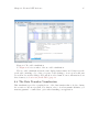
Frontend GUI Reference . . . . . . . . . . . . . . . . . . . . . . 30
8.1
Overview of the PPW GUI . . . . . . . . . . . . . . . . . . . . . . . . . . . . . . . . . . . .
8.1.1 Open File List . . . . . . . . . . . . . . . . . . . . . . . . . . . . . . . . . . . . . . . . . . .
8.1.2 Experiment Information Panel . . . . . . . . . . . . . . . . . . . . . . . . . . . .
8.1.3 Source Panel . . . . . . . . . . . . . . . . . . . . . . . . . . . . . . . . . . . . . . . . . . . . .
8.1.4 Visualization Panel . . . . . . . . . . . . . . . . . . . . . . . . . . . . . . . . . . . . . . .
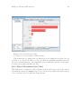
8.2 The Profile Table Visualization . . . . . . . . . . . . . . . . . . . . . . . . . . . . . . . .
8.3 The Tree Table Visualization . . . . . . . . . . . . . . . . . . . . . . . . . . . . . . . . . .
8.4 The Data Transfers Visualization . . . . . . . . . . . . . . . . . . . . . . . . . . . . . .
8.5 The Array Distribution Visualization . . . . . . . . . . . . . . . . . . . . . . . . . .
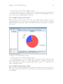
8.6 The Profile Charts Visualization. . . . . . . . . . . . . . . . . . . . . . . . . . . . . . .
8.6.1 Operation Types Pie Chart . . . . . . . . . . . . . . . . . . . . . . . . . . . . . . .
8.6.2 Profile Metrics Pie Chart . . . . . . . . . . . . . . . . . . . . . . . . . . . . . . . . .
8.6.3 Profile Metrics Bar Chart . . . . . . . . . . . . . . . . . . . . . . . . . . . . . . . .
8.6.4 Thread Breakdown Line Chart . . . . . . . . . . . . . . . . . . . . . . . . . . .
8.6.5 Total Times Line Chart . . . . . . . . . . . . . . . . . . . . . . . . . . . . . . . . . .
8.6.6 Total Times by Function . . . . . . . . . . . . . . . . . . . . . . . . . . . . . . . . .
8.7 Analysis Menu . . . . . . . . . . . . . . . . . . . . . . . . . . . . . . . . . . . . . . . . . . . . . . . .
8.7.1 Application Analysis . . . . . . . . . . . . . . . . . . . . . . . . . . . . . . . . . . . . .
8.7.2 Scalability Analysis . . . . . . . . . . . . . . . . . . . . . . . . . . . . . . . . . . . . . .
8.7.3 Memory Leak Analysis . . . . . . . . . . . . . . . . . . . . . . . . . . . . . . . . . . .
8.7.4 Saving Analysis Data . . . . . . . . . . . . . . . . . . . . . . . . . . . . . . . . . . . . .
8.7.5 Load-Balancing Analysis . . . . . . . . . . . . . . . . . . . . . . . . . . . . . . . . .
8.8 Analysis Visualizations . . . . . . . . . . . . . . . . . . . . . . . . . . . . . . . . . . . . . . . .
8.8.1 High Level Application Analysis . . . . . . . . . . . . . . . . . . . . . . . . . .
8.8.2 Experiment Set Analysis . . . . . . . . . . . . . . . . . . . . . . . . . . . . . . . . .
8.8.3 Analysis Table . . . . . . . . . . . . . . . . . . . . . . . . . . . . . . . . . . . . . . . . . . .
8.8.4 Analysis Summary . . . . . . . . . . . . . . . . . . . . . . . . . . . . . . . . . . . . . . .
8.9 Jumpshot Introduction . . . . . . . . . . . . . . . . . . . . . . . . . . . . . . . . . . . . . . . .
30
30
32
32
32
33
34
35
37
38
38
39
39
40
41
43
45
45
46
46
46
46
48
48
49
50
51
51
iii
8.9.1
8.9.2
8.9.3
8.9.4
8.9.5
8.9.6
9
Generating Trace Files . . . . . . . . . . . . . . . . . . . . . . . . . . . . . . . . . . .
Starting Jumpshot . . . . . . . . . . . . . . . . . . . . . . . . . . . . . . . . . . . . . . .
Jumpshot’s Timeline View . . . . . . . . . . . . . . . . . . . . . . . . . . . . . . .
Navigating Through Traces . . . . . . . . . . . . . . . . . . . . . . . . . . . . . . .
Preview States and Preview Arrows . . . . . . . . . . . . . . . . . . . . . .
For More Information . . . . . . . . . . . . . . . . . . . . . . . . . . . . . . . . . . . .
52
53
53
55
56
57
Eclipse PTP Integration . . . . . . . . . . . . . . . . . . . . . . 58
9.1
9.2
9.3
9.4
Overview of Eclipse and Eclipse PTP . . . . . . . . . . . . . . . . . . . . . . . . . .
Installation of Eclipse Tools . . . . . . . . . . . . . . . . . . . . . . . . . . . . . . . . . . .
Creating a UPC Project . . . . . . . . . . . . . . . . . . . . . . . . . . . . . . . . . . . . . . .
Using PPW within Eclipse . . . . . . . . . . . . . . . . . . . . . . . . . . . . . . . . . . . .
Appendix A
API Reference . . . . . . . . . . . . . . . . . . . . 69
A.1 UPC Measurement API . . . . . . . . . . . . . . . . . . . . . . . . . . . . . . . . . . . . . .
A.1.1 UPC API Description. . . . . . . . . . . . . . . . . . . . . . . . . . . . . . . . . . . .
A.1.2 UPC API Examples . . . . . . . . . . . . . . . . . . . . . . . . . . . . . . . . . . . . .
A.1.3 UPC API Notes . . . . . . . . . . . . . . . . . . . . . . . . . . . . . . . . . . . . . . . . .
A.2 SHMEM Measurement API . . . . . . . . . . . . . . . . . . . . . . . . . . . . . . . . . . .
A.2.1 SHMEM API Description . . . . . . . . . . . . . . . . . . . . . . . . . . . . . . . .
A.2.2 SHMEM API Examples. . . . . . . . . . . . . . . . . . . . . . . . . . . . . . . . . .
A.2.3 SHMEM API Notes . . . . . . . . . . . . . . . . . . . . . . . . . . . . . . . . . . . . .
A.3 MPI Measurement API . . . . . . . . . . . . . . . . . . . . . . . . . . . . . . . . . . . . . . .
A.3.1 MPI API Description . . . . . . . . . . . . . . . . . . . . . . . . . . . . . . . . . . . .
A.3.2 MPI API Notes . . . . . . . . . . . . . . . . . . . . . . . . . . . . . . . . . . . . . . . . . .
A.4 C Measurement API . . . . . . . . . . . . . . . . . . . . . . . . . . . . . . . . . . . . . . . . . .
A.4.1 C API Description . . . . . . . . . . . . . . . . . . . . . . . . . . . . . . . . . . . . . . .
A.4.2 C API Examples. . . . . . . . . . . . . . . . . . . . . . . . . . . . . . . . . . . . . . . . .
A.4.3 C API Notes . . . . . . . . . . . . . . . . . . . . . . . . . . . . . . . . . . . . . . . . . . . .
Appendix B
58
58
58
62
69
69
70
72
73
73
73
74
75
75
75
76
76
76
77
Command Reference . . . . . . . . . . . . . 78
B.1 ppw . . . . . . . . . . . . . . . . . . . . . . . . . . . . . . . . . . . . . . . . . . . . . . . . . . . . . . . . . .
B.1.1 Invoking ppw . . . . . . . . . . . . . . . . . . . . . . . . . . . . . . . . . . . . . . . . . . . .
B.1.2 ppw Command Options . . . . . . . . . . . . . . . . . . . . . . . . . . . . . . . . . .
B.1.3 ppw Notes . . . . . . . . . . . . . . . . . . . . . . . . . . . . . . . . . . . . . . . . . . . . . . .
B.1.4 ppw Environment Variables . . . . . . . . . . . . . . . . . . . . . . . . . . . . . .
B.2 ppwjumpshot . . . . . . . . . . . . . . . . . . . . . . . . . . . . . . . . . . . . . . . . . . . . . . . . .
B.2.1 Invoking ppwjumpshot . . . . . . . . . . . . . . . . . . . . . . . . . . . . . . . . . . .
B.2.2 ppwjumpshot Command Options . . . . . . . . . . . . . . . . . . . . . . . . .
B.2.3 ppwjumpshot Notes . . . . . . . . . . . . . . . . . . . . . . . . . . . . . . . . . . . . . .
B.2.4 ppwjumpshot Environment Variables . . . . . . . . . . . . . . . . . . . . .
B.3 ppwprof . . . . . . . . . . . . . . . . . . . . . . . . . . . . . . . . . . . . . . . . . . . . . . . . . . . . . .
B.3.1 Invoking ppwprof . . . . . . . . . . . . . . . . . . . . . . . . . . . . . . . . . . . . . . . .
B.3.2 ppwprof Command Options . . . . . . . . . . . . . . . . . . . . . . . . . . . . . .
B.3.3 ppwprof Notes . . . . . . . . . . . . . . . . . . . . . . . . . . . . . . . . . . . . . . . . . . .
B.3.4 ppwprof Environment Variables . . . . . . . . . . . . . . . . . . . . . . . . . .
B.4 ppwprof.pl. . . . . . . . . . . . . . . . . . . . . . . . . . . . . . . . . . . . . . . . . . . . . . . . . . . .
78
78
78
78
78
79
79
79
79
79
80
80
80
81
81
82
iv
B.4.1 Invoking ppwprof.pl. . . . . . . . . . . . . . . . . . . . . . . . . . . . . . . . . . . . . . 82
B.4.2 ppwprof Command Options . . . . . . . . . . . . . . . . . . . . . . . . . . . . . . 82
B.4.3 ppwprof Notes . . . . . . . . . . . . . . . . . . . . . . . . . . . . . . . . . . . . . . . . . . . 82
B.5 ppwhelp . . . . . . . . . . . . . . . . . . . . . . . . . . . . . . . . . . . . . . . . . . . . . . . . . . . . . . 83
B.5.1 Invoking ppwhelp . . . . . . . . . . . . . . . . . . . . . . . . . . . . . . . . . . . . . . . . 83
B.5.2 ppwhelp Command Options . . . . . . . . . . . . . . . . . . . . . . . . . . . . . . 83
B.5.3 ppwhelp Notes . . . . . . . . . . . . . . . . . . . . . . . . . . . . . . . . . . . . . . . . . . . 83
B.5.4 ppwhelp Environment Variables . . . . . . . . . . . . . . . . . . . . . . . . . . 83
B.6 ppwcc . . . . . . . . . . . . . . . . . . . . . . . . . . . . . . . . . . . . . . . . . . . . . . . . . . . . . . . . 84
B.6.1 Invoking ppwcc . . . . . . . . . . . . . . . . . . . . . . . . . . . . . . . . . . . . . . . . . . 84
B.6.2 ppwcc Command Options . . . . . . . . . . . . . . . . . . . . . . . . . . . . . . . . 84
B.6.3 ppwcc Notes . . . . . . . . . . . . . . . . . . . . . . . . . . . . . . . . . . . . . . . . . . . . . 85
B.7 ppwshmemcc . . . . . . . . . . . . . . . . . . . . . . . . . . . . . . . . . . . . . . . . . . . . . . . . . 86
B.7.1 Invoking ppwshmemcc . . . . . . . . . . . . . . . . . . . . . . . . . . . . . . . . . . . 86
B.7.2 ppwshmemcc Command Options . . . . . . . . . . . . . . . . . . . . . . . . . 86
B.7.3 ppwshmemcc Notes . . . . . . . . . . . . . . . . . . . . . . . . . . . . . . . . . . . . . . 87
B.8 ppwmpicc . . . . . . . . . . . . . . . . . . . . . . . . . . . . . . . . . . . . . . . . . . . . . . . . . . . . 88
B.8.1 Invoking ppwmpicc . . . . . . . . . . . . . . . . . . . . . . . . . . . . . . . . . . . . . . 88
B.8.2 ppwmpicc Command Options . . . . . . . . . . . . . . . . . . . . . . . . . . . . 88
B.8.3 ppwmpicc Notes . . . . . . . . . . . . . . . . . . . . . . . . . . . . . . . . . . . . . . . . . 89
B.9 ppwupcc . . . . . . . . . . . . . . . . . . . . . . . . . . . . . . . . . . . . . . . . . . . . . . . . . . . . . 90
B.9.1 Invoking ppwupcc . . . . . . . . . . . . . . . . . . . . . . . . . . . . . . . . . . . . . . . 90
B.9.2 ppwupcc Command Options . . . . . . . . . . . . . . . . . . . . . . . . . . . . . 90
B.9.3 ppwupcc Notes . . . . . . . . . . . . . . . . . . . . . . . . . . . . . . . . . . . . . . . . . . 91
B.10 ppwrun. . . . . . . . . . . . . . . . . . . . . . . . . . . . . . . . . . . . . . . . . . . . . . . . . . . . . . 93
B.10.1 Invoking ppwrun . . . . . . . . . . . . . . . . . . . . . . . . . . . . . . . . . . . . . . . 93
B.10.2 ppwrun Command Options . . . . . . . . . . . . . . . . . . . . . . . . . . . . . 93
B.10.3 ppwrun Notes . . . . . . . . . . . . . . . . . . . . . . . . . . . . . . . . . . . . . . . . . . 95
B.10.4 ppwrun Environment Variables . . . . . . . . . . . . . . . . . . . . . . . . . 97
B.11 par2cube . . . . . . . . . . . . . . . . . . . . . . . . . . . . . . . . . . . . . . . . . . . . . . . . . . . . 98
B.11.1 Invoking par2cube . . . . . . . . . . . . . . . . . . . . . . . . . . . . . . . . . . . . . . 98
B.11.2 par2cube Command Options . . . . . . . . . . . . . . . . . . . . . . . . . . . . 98
B.11.3 par2cube Notes . . . . . . . . . . . . . . . . . . . . . . . . . . . . . . . . . . . . . . . . . 98
B.11.4 par2cube Environment Variables . . . . . . . . . . . . . . . . . . . . . . . . 98
B.12 par2tau . . . . . . . . . . . . . . . . . . . . . . . . . . . . . . . . . . . . . . . . . . . . . . . . . . . . . 99
B.12.1 Invoking par2tau . . . . . . . . . . . . . . . . . . . . . . . . . . . . . . . . . . . . . . . 99
B.12.2 par2tau Command Options . . . . . . . . . . . . . . . . . . . . . . . . . . . . . 99
B.12.3 par2tau Notes . . . . . . . . . . . . . . . . . . . . . . . . . . . . . . . . . . . . . . . . . . 99
B.12.4 par2tau Environment Variables . . . . . . . . . . . . . . . . . . . . . . . . . 99
B.13 par2yaml . . . . . . . . . . . . . . . . . . . . . . . . . . . . . . . . . . . . . . . . . . . . . . . . . . . 100
B.13.1 Invoking par2yaml . . . . . . . . . . . . . . . . . . . . . . . . . . . . . . . . . . . . . 100
B.13.2 par2yaml Command Options . . . . . . . . . . . . . . . . . . . . . . . . . . 100
B.13.3 par2yaml Notes. . . . . . . . . . . . . . . . . . . . . . . . . . . . . . . . . . . . . . . . 100
B.14 par2otf . . . . . . . . . . . . . . . . . . . . . . . . . . . . . . . . . . . . . . . . . . . . . . . . . . . . . 101
B.14.1 Invoking par2otf . . . . . . . . . . . . . . . . . . . . . . . . . . . . . . . . . . . . . . . 101
B.14.2 par2otf Command Options. . . . . . . . . . . . . . . . . . . . . . . . . . . . . 101
B.14.3 par2otf Notes . . . . . . . . . . . . . . . . . . . . . . . . . . . . . . . . . . . . . . . . . . 101
B.14.4 par2otf Environment Variables . . . . . . . . . . . . . . . . . . . . . . . . . 101
v
B.15 par2slog2. . . . . . . . . . . . . . . . . . . . . . . . . . . . . . . . . . . . . . . . . . . . . . . . . . .
B.15.1 Invoking par2slog2. . . . . . . . . . . . . . . . . . . . . . . . . . . . . . . . . . . . .
B.15.2 par2slog2 Command Options . . . . . . . . . . . . . . . . . . . . . . . . . .
B.15.3 par2slog2 Notes . . . . . . . . . . . . . . . . . . . . . . . . . . . . . . . . . . . . . . .
B.15.4 par2slog2 Environment Variables . . . . . . . . . . . . . . . . . . . . . .
B.16 ppw-config . . . . . . . . . . . . . . . . . . . . . . . . . . . . . . . . . . . . . . . . . . . . . . . . .
B.16.1 Invoking ppw-config . . . . . . . . . . . . . . . . . . . . . . . . . . . . . . . . . . .
B.16.2 ppw-config Command Options . . . . . . . . . . . . . . . . . . . . . . . . .
B.17 ppw-showopts . . . . . . . . . . . . . . . . . . . . . . . . . . . . . . . . . . . . . . . . . . . . . .
B.17.1 Invoking ppw-showopts . . . . . . . . . . . . . . . . . . . . . . . . . . . . . . . .
B.17.2 ppw-showopts Command Options . . . . . . . . . . . . . . . . . . . . . .
B.18 ppwresolve.pl . . . . . . . . . . . . . . . . . . . . . . . . . . . . . . . . . . . . . . . . . . . . . . .
B.18.1 Invoking ppwresolve.pl . . . . . . . . . . . . . . . . . . . . . . . . . . . . . . . . .
B.18.2 ppwresolve.pl Command Options . . . . . . . . . . . . . . . . . . . . . .
B.18.3 ppwresolve.pl Notes . . . . . . . . . . . . . . . . . . . . . . . . . . . . . . . . . . .
B.19 ppwparutil.pl . . . . . . . . . . . . . . . . . . . . . . . . . . . . . . . . . . . . . . . . . . . . . . .
B.19.1 Invoking ppwparutil.pl . . . . . . . . . . . . . . . . . . . . . . . . . . . . . . . . .
B.19.2 ppwparutil.pl Command Options . . . . . . . . . . . . . . . . . . . . . .
B.20 ppwcomminfo.pl . . . . . . . . . . . . . . . . . . . . . . . . . . . . . . . . . . . . . . . . . . . .
B.20.1 Invoking ppwcomminfo.pl . . . . . . . . . . . . . . . . . . . . . . . . . . . . . .
B.20.2 ppwcomminfo.pl Command Options. . . . . . . . . . . . . . . . . . . .
102
102
102
102
102
103
103
103
104
104
104
105
105
105
105
106
106
106
107
107
107
Concept Index. . . . . . . . . . . . . . . . . . . . . . . . . . . . . . . . . . . . 108
PPW User Manual
1
PPW User Manual
Thank you for downloading the Parallel Performance Wizard (PPW) tool, version 3.2. This
user manual describes how to install and use PPW.
We hope that you find PPW useful for troubleshooting performance problems in your
applications. Should you encounter any problems while using PPW, please report them
using our Bugzilla website. You may also report feature requests using this website. We
want our software to remain as bug-free as possible and appreciate any feedback that might
help us improve our tool.
If this is your first time using PPW or you are not very familiar with PPW, we recommend reading the PPW concepts chapter (see Chapter 1 [PPW Concepts], page 2) first.
Chapter 1: PPW Concepts
2
1 PPW Concepts
Welcome to the wonderful world of parallel performance analysis! As you may have already
learned, getting a significant fraction of your hardware’s peak performance is a challenging
enough task for a single-CPU system, and trying to tune the performance of parallel applications can become overwhelming unless you have a tool to help you along your way. If
you’re reading this manual, then you’re already on the right track.
First of all, we’ll start with a brief background to experimental performance analysis,
that is, analyzing your application by running performance experiments. If you’re already
familiar with performance analysis or performance tools, you can skip most of the rest of
this section, although we do recommend that you glance through this section so that you
are aware of the terminology that the rest of this manual uses.
Next, we’ll overview some terminology related to different methods of collecting profile
data. Feel free to skim through this section at first, but you may wish to read it more
thoroughly after you’ve become more familiar with PPW.
Finally, we’ll quickly describe PPW’s general workflow. We highly recommend reading
this section, especially if you have never used PPW before.
1.1 Introduction to Performance Analysis
In experimental performance analysis, there are two major techniques that influence the
overall design and workflow of performance tools. The first technique, profiling, keeps track
of basic statistical information about a program’s performance at runtime. This compact
representation of a program’s execution is usually presented to the developer immediately
after the program has finished executing, and gives the developer a high-level view of where
time is being spent in their application code. The second technique, tracing, keeps a complete log of all activities performed by a developer’s program inside a trace file. Tracing
usually results in large trace files, especially for long-running programs. However, tracing
can be used to reconstruct the exact behavior of an application at runtime. Tracing can also
be used to calculate the same information available from profiling and so can be thought of
as a more general performance analysis technique.
Performance analysis in performance tools supporting either profiling or tracing is usually carried out in five distinct stages: instrumentation, measurement, analysis, presentation, and optimization. Developers take their original application, instrument it to record
performance information, and run the instrumented program. The instrumented program
produces raw data (usually in the form of a file written to disk), which the developer gives
to the performance tool to analyze. The performance tool then presents the analyzed data
to the developer, indicating where any performance problems exist in their code. Finally,
developers change their code by applying optimizations and repeat the process until they
achieve acceptable performance. This collective process is often referred to as the measuremodify approach, and each stage will be discussed in the remainder of this section.
1.1.1 Instrumentation
During the instrumentation stage, an instrumentation entity (either software or a developer) inserts code into a developer’s application to record when interesting events happen,
such as when communication or synchronization occurs. Instrumentation may be accomplished in one of three ways: through source instrumentation, through the use of wrapper
Chapter 1: PPW Concepts
3
libraries, or through binary instrumentation. While most tools may use only one of these
instrumentation techniques, it is possible to use a combination of techniques to instrument
a developer’s application.
Source instrumentation places measurement code directly inside a developer’s source
code files. While this enables tools to easily relate performance information back to the developer’s original lines of source code, modifying the original source code may interfere with
compiler optimizations. Source instrumentation is also limited because it can only profile
parts of an application that have source code available, which can be a problem when users
wish to profile applications that use external libraries distributed only in compiled form.
Additionally, source instrumentation generally requires recompiling an entire application
over again, which is inconvenient for large applications.
Wrapper libraries use interposition to record performance data during a program’s execution and can only be used to record information about calls made to libraries such as
MPI. Instead of linking against the original library, a developer first links against a library
provided by a performance tool and then links against the original library. Library calls
are intercepted by the performance tool library, which passes on the call to the original
library after recording information about each call. In practice, this interposition is usually accomplished during the linking stage by including weak symbols for all library calls.
Wrapper libraries can be convenient because developers only need to re-link an application
against a new library, which means that there is less interference with compiler optimizations. However, wrapper libraries are limited to capturing information about each library
call. Additionally, many tools that use wrapper libraries cannot relate performance data
back to the developer’s source code (eg, locations of call sites to the library). Wrapper
libraries are used to implement the MPI profiling interface (PMPI), which is used by most
performance tools to record information about MPI communication.
Binary instrumentation is the most convenient instrumentation technique for developers,
but places a high technical burden on performance tool writers. This technique places instrumentation code directly into an executable, requiring no recompilation or relinking. The
instrumentation may be performed before runtime, or may happen dynamically at runtime.
Additionally, since no recompiling or relinking is required, any optimizations performed by
the compiler are not lost. The major problem with binary instrumentation is that it requires
substantial changes to support new platforms, since each platform generally has completely
different binary file formats and instruction sets. As with wrapper libraries, mapping information back to the developer’s original source code can be difficult or impossible, especially
when no debugging symbols exist in the executable.
Our PPW performance tool uses a variety of the above techniques to instrument UPC
and SHMEM programs. For UPC programs, we rely on tight integration with UPC compilers by way of the GASP performance tool interface, which is described in detail at the
GASP website. For the most part, the instrumentation technique used by PPW should be
transparent to most users.
1.1.2 Measurement
In the measurement stage, data is collected from a developer’s program at runtime. The
instrumentation and measurement stages are closely related; performance information can
only be directly collected for parts of the program that have been instrumented.
Chapter 1: PPW Concepts
4
The term metric is used to describe what kind of data is being recorded during the
measurement phase. The most common metric collected by performance tools is the wall
clock time taken for each portion of a program, which is simply the elapsed time as reported
by a standard clock that might hang on your wall. This timing information can be further
separated into time spent on communication, synchronization, and computation. In addition to wall clock time, a performance tool can also record the number of times a certain
event happens, the amount of bytes transferred during communication, and other metrics.
Many tools also use hardware counter libraries such as PAPI to record hardware-specific
information such as cache miss counts.
There is an obvious tradeoff between the amount of data that can be collected and the
overhead imposed by collecting this data. In general, the more information collected during
runtime, the more overhead experienced and thus the less accurate this data becomes.
While early work has shown that it is possible to compensate for much of this overhead
(Allen Malony’s PhD thesis, Performance Observability, is a good starting reference on this
subject), overhead compensation has not become available for the majority of performance
tools.
Profiling tools may also use an indirect method known as sampling to gather performance
information. Instead of using instrumentation to directly measure each event as it occurs
during runtime, metrics such as a program’s callstack are sampled. This sampling can be
performed at fixed intervals, or can be triggered by hardware counter overflows. Using
sampling instead of a more direct measuring technique drastically reduces the amount of
data that a performance tool must analyze. However, sampled data tends to be much
less accurate than performance data collected by direct measurement, especially when the
sampling interval is large enough to miss short-lived events that happen frequently.
Another major advantage of sampling is that sampling does not generally require instrumentation code to be inserted in a program’s performance-critical path. In some instances,
especially in cases where fine-grained performance data is being recorded, this extra instrumentation code can greatly change a program’s runtime behavior.
PPW supports both tracing and profiling modes, but does not support a sampling mode
(although might support a sampling mode in the future if enough users request one). A
future version of PPW will have overhead compensation functionality; if you experience
large overhead while running your application code with PPW, see Chapter 7 [Managing
Overhead], page 26 for techniques on how to manage this overhead.
1.1.3 Analysis
During the analysis stage, data collected during runtime is analyzed in some manner. In
some profiling or sampling tools, this analysis is carried out as the program executes. This
technique is generally referred to as online analysis. More commonly, analysis is deferred
until after an application has finished execution so that runtime overhead is minimized.
Performance tools using this technique are often referred to as post-mortem analysis tools.
The types of analysis capabilities offered varies significantly from tool to tool. Some
performance tools offer no analysis capabilities at all, while others can compute only basic
statistical information to summarize a program’s execution characteristics. A few performance tools offer sophisticated analysis techniques that can identify performance bottlenecks. Generally, tools that provide minimal analysis capabilities rely on the developer to
interpret data shown during the presentation stage.
Chapter 1: PPW Concepts
5
PPW currently has a few simple analysis features, with plans to offer more in the future.
In some modes, PPW will do a small amount of processing and analysis online, but should
be considered a post-mortem analysis tool.
1.1.4 Presentation
After data has been analyzed by the performance tool, the tool must present the data to
the developer for interpretation in the presentation stage.
For tracing tools, the performance tool generally presents the data contained in the
trace file in the form of a space-time diagram, also known as a timeline diagram. In
timeline diagrams, each node in the system is represented by a line. States for each node
are represented through color coding, and communication between nodes is represented by
arrows. Timeline diagrams give a precise recreation of program state and communication
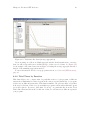
at runtime. The Jumpshot-4 trace visualization tool is a good example of a timeline viewer
(see Section 8.9 [Jumpshot Introduction], page 51 for an introduction to Jumpshot).
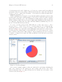
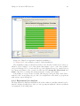
For profiling tools, the performance tool generally displays the profile information in
the form of a chart or table. Bar charts or histograms graphically display the statistics
collected during execution. Text-based tools use formatted text tables to display the same
type of information. A few profiling tools also display performance information alongside
the original source code, as profiled data such as the percentage of time an instruction
contributes to overall execution time lends itself well to this kind of display.
All of PPW’s presentation visualizations are described later in this manual (see Chapter 8
[Frontend GUI Reference], page 30).
1.1.5 Optimization
In most performance tools, the optimization stage in which the code for the program is
changed to improve performance based on the results of the previous stages is left up to
the developer. The majority of performance tools do not have any facility for applying
optimizations to a developer’s code. At best, the performance tool may indicate where a
particular bottleneck occurs in the developer’s source code and expects the developer to
come up with an optimization to apply to their code.
PPW does not have any automated optimization features, although primitive optimization capabilities may be added in the future. Automated optimization is patently difficult
(as witnessed by the nonexistence of practical tools exhibiting this feature). Instead of
being designed as a automated tool with limited real-world utility, PPW has instead been
designed with the aim of enabling users to identify and fix bottlenecks in their programs as
quickly as possible.
1.2 Profile Terminology
As mentioned in the previous section, while collecting full trace data results in a more accurate picture of a program’s runtime behavior, profile data can be collected more efficiently
and managed much more easily. Since profile data is essentially a statistical description of
a program’s runtime performance, a natural question to ask is
How exactly is this performance data being summarized?
While there are many, many different methods that one can use to process performance
data, there are a few popular methods that show up across different tools that we’ll describe
Chapter 1: PPW Concepts
6
in this section. We feel that it is important to understand these terms so that profile data
reported by PPW can be correctly interpreted.
Where possible, we’ve used the same terms that we’ve found in literature to describe the
concepts in this section, although some terms do vary slightly from author to author.
1.2.1 Flat and Full Profiles
Within the category of profiling tools, there are variations on how profile data is collected
with regards to a program’s callstack. Traditionally, profile data is tracked with respect to
the topmost entry on the callstack, which gives a flat profile. Flat profiles keep track of
time spent in each function, but do not keep track of the relationship between functions.
For instance, a flat profile will be able to tell you that your program spent 25.2 seconds
executing function ‘A’, but will not be able to tell you that ‘A’ ran for 10.5 seconds when
called from ‘B’ and 14.7 seconds when called from ‘C’. In other words, a flat profile tallies
time spent with respect to functions rather than function callstacks.
Generating a path profile (also known as a callpath profile) involves another method
of collecting profile data in which statistical information is kept with respect to function
callstacks. A path profile tracks time spent in function paths rather than just time spent
in each function. It is important to point out that a flat profile can be constructed from a
path profile, but not vice versa. Path profiles contain much more useful information at the
cost of higher implementation complexity and storage space for the profile data.
A good way to think of the difference between a flat profile and a path profile is to
logically envision how data is recorded under each scenario. Assume we have the following
C program:
void B() {
sleep(1);
}
void A() {
sleep(1);
B();
}
int main() {
A();
sleep(1);
B();
B();
return 0;
}
In the program above, we see that ‘main’ calls ‘A’, which calls ‘B’. ‘main’ then calls ‘B’
twice, and finally finishes executing.
If we were constructing a flat profile for the above program, we would keep a timer
associated with each function, starting the timer when the function began executing and
stopping the timer when the function returned. Therefore, we would have a total of three
timers: a timer for ‘main’, a timer for ‘A’, and a timer for ‘B’. It is also important to note
Chapter 1: PPW Concepts
7
here that since we are creating an execution profile, we do not create a new timer for each
function each time it executes; rather, we continue tallying with our existing timer if a
function is executed more than once.
If we were constructing a path profile for the above program, we would look up which
timer based on all of the functions on the callstack rather than just the currently-executing
function. Following the execution path above, we would end up with four timers instead of
three: ‘main’, ‘main - A’, ‘main - A - B’, and ‘main - B’. There will be one timer for each
possible callstack, and since we are generating profile data our timers are reused, as with
flat profiles.
Similar to the idea of using function callstacks to track profile data separately, one can
also get more detailed performance information by tracking data with respect to a sequence
of functions with callsite information rather than a sequence of function names. Profiles
based on callsites are sometimes called callsite profiles. Continuing with our example above,
we would end up with five timers: ‘main’ with no callsite, ‘main - A’ with a callsite in ‘main’,
‘main - A - B’ with a callsite in ‘A’, ‘main - B’ with one callsite in ‘main’, and ‘main - B’
with a second callsite in ‘main’. In short, we end up with nearly the same group of timers as
with a path profile, except that we end up with an additional timer for ‘main - B’ because
it is called from two different lines of code within ‘main’.
Note that the TAU performance tool framework uses a slightly different definition of
the term “callpath profile”. In TAU’s version of callpath profiles, timers are differentiated
based on looking at a maximum of N entries from the bottom of the callstack to the root.
A TAU callpath profile with a depth of two for the example given above would have the
following timers: ‘main’, ‘main - A’, ‘main - B’, and ‘A - B’. TAU uses the term calldepth
profile to refer to PPW’s path profiles, which is really just a special case of a TAU callpath
profile with an infinite depth.
PPW’s measurement code will always collect full path profiles rather than flat profiles,
and uses callsite profiles.
In PPW, the profile table visualization shows a flat profile and the tree table visualization
shows path profiles. The flat profile information is calculated from the full callpath profile,
and timers are grouped together by region where appropriate (when they have no subcalls).
1.2.2 Phases and Regions
There are many definitions of the term program phase, but for the purposes of this manual
we use the term to describe a time interval in which a program is performing a particular activity. For a linear algebra application, example phases might include matrix initialization,
Eigenvalue computation, doing a matrix-vector product, collecting results from all nodes,
formatting output, and performing disk I/O to write the results of all computations to disk.
Each program phase generally has different performance characteristics, and for this reason
it is generally useful to treat each phase as a separate entity during the performance tuning
process.
The idea of keeping track of timers for each function can be extended to track arbitrary
sections of program code. A program region, also called a region, is a generalization of the
function concept that may include loops and sections of functions. Additionally, regions
may span groups of functions. The concept of a region is useful for attributing performance
information to particular phases of program execution.
Chapter 1: PPW Concepts
8
When working with regions, it is possible to have a region that contains other regions,
such as a ‘for’ loop within a function. These regions are referred to as subregions, because
they are regions contained within another region.
In most cases, the terms region and function can be used interchangeably. PPW and
the rest of this manual use the more general term region instead of function; feel free to
mentally substitute “function” for “region” and “function call” for “subregion call” when
reading this manual.
To track phase data and arbitrary regions of code, PPW exposes a user-level measurement API (see Appendix A [API Reference], page 69 for details on how to use this API
within your programs).
When compiling using the ‘--inst-functions’ option to ‘ppwcc’, ‘ppwshmemcc’, or
‘ppwupcc’, PPW will automatically instrument your program to track function entry and
exit for compilers that support this. In this case, regions representing functions in your program will be created automatically at runtime by PPW’s measurement code. See Section B.6
[ppwcc], page 84, Section B.7 [ppwshmemcc], page 86, and Section B.9 [ppwupcc], page 90
for more information on those commands. Note that the ‘--inst-functions’ option is not
supported on all compilers.
PPW always creates a toplevel region named ‘Application’ that keeps track of the total
execution time of the program.
1.2.3 Inclusive and Exclusive Times
Profile data may also differentiate between time spent executing within a region and time
spent in calls to other region within a given region. Time spent executing code in the
region itself is referred to as exclusive time or self time. Time spent within this region and
any subregion calls (ie, function calls) is referred to as inclusive time or total time. The
inclusive/exclusive terms can be easily differentiated with the following sentence:
Exclusive time for function ‘A’ is the time spent executing statements in the
body of ‘A’, while inclusive time is the total time spent executing ‘A’ including
any subroutine calls.
PPW uses the self/total terms because they are easier to remember: self time is only the
time taken by the region itself, and total refers to all the time taken by a region including
any subregions or calls to other regions.
1.2.4 Other Profile Statistics
Sometimes it is useful to know how many times a particular region was executed, or how
many times a region made calls to other regions or executed subregions within that region.
Such statistics are useful in identifying functions that might benefit from inlining. These
terms are usually known as calls and sub calls, although some other tools use the term
count instead.
Many times, when troubleshooting a load-balancing problem in which a region of code
has input-sensitive execution time, it is useful to know the minimum and maximum time
spent executing a particular region. Tracking min time and max time can be done using
either inclusive or exclusive time, but most tools usually track min and max statistics for
inclusive time since it generally is easier to interpret.
Chapter 1: PPW Concepts
9
In addition to calls and min/max time, other summary statistics about program execution can also be collected, including standard deviation of inclusive times and average
exclusive or inclusive time (which can be derived from other statistics).
PPW does keep track of call and sub call counts, in addition to min and max time. However, for overhead management reasons, PPW does not track any other statistics. If you’d
like to see PPW track other statistics, please file a bug report for a feature enhancement
using the Bugzilla website.
1.2.5 Aggregating Profile Data
Armed with the terms above, we can now discuss one of the stranger topics relating to
profile data, which is how to interpret profile data spanning different nodes. While tools
can simply display profile data for each node, this amount of data becomes impractical
after only a few nodes. Instead, most tools choose to aggregate the data in some manner
by combining the data using one of several techniques.
The most straightforward method of aggregating data from different nodes is to simply
sum together timers that have the same callpath. When summing profile data in this
manner, the resulting profile gives you a good overall picture of how time (or whatever
metric was collected) was spent in your application across every node. Interpreting summed
profile data is fairly straightforward, as it will show any regions of code that contributed a
significant amount to overall runtime. In addition, looking at summed profile data will also
identify any costly synchronization constructs that sap program efficiency.
Other aggregation methods including taking the min, max, or average metric values
across each timer with the same callpath. These aggregation techniques give performance
data that is representative of a single node in the system, instead of giving a summary
of data across all nodes. While aggregating the data using these techniques can give you
a little more insight into the distribution of values among regions in your program, the
resulting data can often be slightly strange.
For example, let’s assume you have a simple program with three functions ‘main’, ‘A’,
and ‘B’. In this example, ‘main’ makes a single call to both ‘A’ and ‘B’ and does not do
anything aside from calling ‘A’ and ‘B’. A flat profile for this example might look like this
(with times reported in seconds):
Node
Region
Inclusive time
Exclusive time
---------------------------------------------------1
main
10.0
0.0
1
A
7.5
7.5
1
B
2.5
2.5
2
main
10.0
0.0
2
A
2.5
2.5
2
B
7.5
7.5
If we aggregate using summing, the resulting profile would look like this:
Region
Inclusive time
Exclusive time
-------------------------------------------main
20.0
0.0
A
10.0
10.0
Chapter 1: PPW Concepts
10
B
10.0
10.0
which makes sense, although glosses over the fact that ‘A’ and ‘B’ took different times to
execute on different nodes. Note that by aggregating data together, we always lose some
of these details, although tools providing a breakdown of an aggregated metric across all
nodes will let you reconstruct this information.
Now let’s look at what the data will look like if we aggregate using the max values:
Region
Inclusive time
Exclusive time
-------------------------------------------main
10.0
0.0
A
7.5
7.5
B
7.5
7.5
This data set definitely looks much stranger, especially if you consider that it is telling you
the sum of time spent in ‘A’ and ‘B’ is greater than all time spent in ‘main’. However, this
data set also lets us know that both ‘A’ and ‘B’ took a max of 7.5 seconds to execute on at
least one node, which is useful to know as the time can be treated as a “worst-case” time
across all nodes.
A similar thing happens when we aggregate using min values:
Region
Inclusive time
Exclusive time
-------------------------------------------main
10.0
0.0
A
2.5
2.5
B
2.5
2.5
Similar to the max aggregation example, the min values give us the “best-case” time for
executing that region across all nodes, which is somewhat unintuitive.
When aggregating data using path profiles rather than flat profiles, these oddities make
the resulting data set even harder to interpret properly. Since a function hierarchy can
be reconstructed from path profile information, a tool can feasibly “fix” the aggregation
by recalculating inclusive times in a bottom-up fashion based on the new exclusive timing
information. However, after “fixing” this data, one could argue that the data set is no
longer representative of the original program run.
To summarize, the summing aggregation technique is the most useful because the resulting data is simply a summary of all node data in the system. The min and max aggregation
techniques can be used to get an idea of the best- and worst-case performance data that
could be expected from any node in the system, and the averaging technique can be used
to get an idea of nominal performance data for any given node in the system.
As mentioned before, given a path profile, we can use aggregation techniques to derive
a flat profile. In this case, it only makes sense to use a summing aggregation, as the
min/max/average techniques make the resulting data set nonsensical.
PPW offers all four aggregation techniques described here, but uses summing as a default
aggregation method since it is the easiest to make sense of. For the profile table visualization, PPW uses the summing aggregation technique on single-node path profile data.
Additionally, when aggregating other profile statistics such as calls and max inclusive time,
PPW uses the expected method (summing counts, taking the absolute min of all minimum
Chapter 1: PPW Concepts
11
times and the absolute max of all maximum times, etc). Also, when aggregating path profiles, PPW does not attempt to “fix” inclusive times and instead shows the inclusive times
generated by the aggregation method itself.
1.3 High-Level Description of PPW’s Workflow
In designing PPW, we have strived to make day-to-day usage of our tool to be as painless
as possible. Rather than require users to completely modify their build process, we have
opted to use compiler wrapper scripts that take care of the mundane details of setting
up PPW’s compilation environment. Also, our tool has been designed to work with both
batch-processing and interactive machines, so we have taken the approach of providing a
text-based interface (via the ppwprof command) for viewing performance data on your
parallel machine, in addition to a graphical frontend that can run both on your parallel
machine (the ppw command) and on your workstation.
In general, and assuming you have a working installation of PPW (see Chapter 2 [Installing PPW], page 12), to use PPW you generally perform these steps:
• Instead of using upcc or cc (ie, your regular compilers), compile your application using
ppwupcc for UPC programs, ppwshmemcc for SHMEM programs, or ppwcc for sequential
C programs.
• Prefix your regular run command with ‘ppwrun --profile’ to gather profile data or
‘ppwrun --trace’ to gather trace data.
• View performance information using ppwprof or by transferring the PAR data file to
your workstation and using the PPW GUI. If you’ve collected trace data, then convert
your PAR data file using one of the conversion utilities and view your performance
data in Jumpshot or Vampir.
• Update your code and run your program again to see how your application’s performance changed.
• Repeat until your application is fast/efficient enough.
More details on each of the steps listed above can be found in later parts in this manual.
Chapter 2: Installing PPW
12
2 Installing PPW
We have designed our tool to integrate well with batch processing and interactive systems.
To support both types of environments, we’ve split our tool into two pieces: a frontend used
for browsing performance data on your workstation, and a backend that interfaces with your
application and system libraries. The rest of this chapter will explain how to install both
the frontend and backend of our tool onto your workstation and parallel machine.
2.1 Installing the Frontend
The frontend has a graphical user interface written in Java, so you’ll need a relatively recent
installation of the Java Runtime Environment (JRE). Our frontend requires Java version
1.5 or above. If you don’t have a recent JRE installed, you can install one (for free, of
course!) by visiting the Java website. Once you’ve installed the JRE, you can download an
appropriate installer for your workstation by visiting the PPW website.
2.2 Installing the Backend
Our backend is distributed in source code form, which means to install it you’ll need to
compile it first. We use the standard open-source Automake and Autoconf tools to help
you configure the package for your system. If you’ve never heard of these before, don’t
worry; all you need to do is follow the instructions outlined in the rest of this section.
If you compile and install the source code distribution of PPW, both the frontend and
the backend will be installed. If the machine on which you are installing PPW does not have
Java support (eg, if you are unable to find a JVM for it, or do not have permissions to install
a JVM), a few commandline tools will be unavailable. However, functional equivalents of
these commandline tools are available through the GUI on your workstation, and none of
these tools are required to operate the tool.
A word about portability: the backend of our tool is written in portable ANSI C and
should compile on just about any UNIX-like system. If you have problems compiling or
installing our software on your machine, please file a bug report at our Bugzilla website and
we’ll work with you to get our tool working on your system.
2.2.1 Backend Prerequisites
There are a number of prerequisites (system requirements) which you will need in order to
build the PPW software. At a minimum, you will need the following:
• Some version of Unix, or a Unix-like operating environment
• make (GNU make is recommended)
• Perl (5.005 or newer)
• A number of standard Unix tools: a Bourne-compatible shell, ’sed’, ’awk’, etc.
• A C compiler. The PPW code should be able to build with essentially any C89compliant compiler. Let us know if you find an exception.
Before you can install our tool, you’ll need to have a version of a UPC compiler, a
SHMEM library, or an MPI library that our tool supports on your system. Currently,
PPW supports the following parallel programming languages/libraries:
Chapter 2: Installing PPW
13
• Berkeley UPC version 2.3.16+ configured with instrumentation enabled (using
‘--with-multiconf=+opt_inst’ for newer versions of Berkeley UPC, or the
‘--enable-inst’ flag for older versions)
• GCC UPC version 4.3.2.4+
• A recent version of HP UPC (released in or after 2011)
• A version of Quadrics SHMEM containing PSHMEM support (any version of QSNET2LIBS 2.2.8+ should work)
• A version of the MPI library
If your favorite UPC compiler isn’t on the list above, please contact your vendor and
request that they add support for the GASP performance tool interface as described on the
GASP website.
If your favorite parallel programming library isn’t on the list above, please contact us
and we’ll try our best to add support for it.
2.2.2 Compiling the Backend
To compile the backend, you’ll need to download the PPW source distribution from the
PPW website onto your system, and then uncompress and untar it.
Once you’ve expanded the source distribution, you’ll need to run the configure script
to adapt the tool to your system. If you’ve installed your UPC or SHMEM libraries in
nonstandard locations, you might have to provide the configure script with additional arguments. For MPI, you’ll need to use a configure option to specify the location of the MPI
installation you would like to use. You may type ‘./configure --help’ to see what options
are available; here’s a quick guide to help you get started:
• ‘--with-upc=DIR’: If you’ve installed your UPC compiler in a nonstandard location,
use this option to tell the tool in which directory you’ve installed your UPC compiler,
such as --with-upc=/usr/local/berkeley-upc-2.8.0. By default, PPW will try to
find your UPC compiler automatically, but if it doesn’t find it or finds the wrong one,
use this option.
• ‘--with-mpi=DIR’: This option tells PPW where to find the MPI installation you would
like to use for analyzing MPI programs. This option is currently required in order to
use MPI with PPW.
• ‘--with-papi=DIR’: Similar to above, if you have the PAPI hardware counter library
installed on your system and PPW doesn’t find it, use this option to point PPW to
where you installed PAPI. For more information on the PAPI library, please refer to the
PAPI website. Note that PPW requires PAPI version 3 or higher. We highly recommend that you install PAPI on your systems as hardware counters can be indispensable
in the tuning process; however, be warned that installing PAPI can be a very involved
process. Bribing your local system administrator with free pizza might go a long way
for you. . .
• ‘--prefix=DIR’: If you don’t have root privileges on your machine, or would like to
install PPW in another directory than the default, you can use this option to customize
where PPW will be installed. This option is typically used to install software into
your home directory rather than into system directories. If you use this option, you’ll
probably have to edit your PATH environment variable so that you don’t have to specify
the full path to the PPW commandline programs and scripts.
Chapter 2: Installing PPW
14
• ‘--with-mpiP=DIR’: For GASP implementations that don’t provide source code information directory (such as PPW’s support for SHMEM and sequential C), PPW can
use the mpiP library to get this information. To do this, point PPW at your mpiP installation directory (eg, ‘/usr/local/mpiP/’). You’ll need mpiP version 2.8.2 or above
installed for this to work.
Note that mpiP is very sensitive to compiler optimizations. In particular, you need to
compile mpiP with no optimizations and compile your application with no optimizations and debug flags in order for mpiP’s callsite support to work reliably.
As with using mpiP by itself, when you link your application, you’ll need to specify all
the libraries that mpiP requires. This usually includes ‘-liberty -lbfd’ and the like.
For more information, refer to the mpiP website.
If you’re using PPW only for its UPC support, you probably don’t need this option.
• ‘--with-libunwind=DIR’: Use libunwind for getting callsite information. This is similar to the ‘--with-mpiP’ option, except that it enables PPW to use libunwind instead
of mpiP for getting callsite information.
When PPW is configured to use libunwind, resulting PAR files will initially contain
source code information given as virtual memory addresses like ‘0x80497f7’. PPW will
attempt to automatically resolve these addresses using its Section B.18 [ppwresolve.pl],
page 105 utility, which itself invokes the addr2line utility (part of GNU Binutils).
When using libunwind, don’t forget to compile your applications with debug symbols.
This is usually accomplished by passing the ‘-g’ option to most compilers.
On some platforms, you may have to set extra environment variables such as LD_
LIBRARY_PATH in order to get applications compiled against libunwind to run properly.
For more information on libunwind, please visit the libunwind website.
If you’re using PPW only for its UPC support, you probably don’t need this option.
Once the configure script finishes running, the script will tell you what software was found
and how PPW was configured. If you notice something missing, delete the ‘config.cache’
file and re-run the configure script with the correct arguments.
Note: Failure to remove the ‘config.cache’ file when giving new arguments
to the configure script may result in your new configuration options not being
reflected.
After you’ve configured PPW to your liking, type make to compile the tool and make
install to install it. Note that PPW may require GNU make to build correctly. If your
vendor-supplied version of make fails to build PPW properly, we recommend downloading
GNU make from the GNU make website.
2.2.3 Backend Build Session Example
The example session below shows how to download, build, and install PPW:
$ wget "http://ppw.hcs.ufl.edu/v3.2/ppw-3.2.tar.gz"
--18:44:49-- http://ppw.hcs.ufl.edu/v3.2/ppw-3.2.tar.gz
=> ‘ppw-3.2.tar.gz’
Resolving ppw.hcs.ufl.edu... 128.227.45.2
Connecting to ppw.hcs.ufl.edu|128.227.45.2|:80... connected.
HTTP request sent, awaiting response... 200 OK
Chapter 2: Installing PPW
15
Length: 8,297,910 (7.9M) [application/x-tar]
100%[======================================>] 8,297,910
10.80M/s
18:44:50 (10.80 MB/s) - ‘ppw-3.2.tar.gz’ saved [8297910/8297910]
$ gunzip -c ppw-3.2.tar.gz | tar xf $ cd ppw-3.2
$ ./configure --prefix=/home/ACCT/ppw
... output truncated ...
$ make; make install
After these commands finish executing, PPW will be installed in ‘/home/ACCT/ppw’.
Remember to replace ‘ACCT’ with your username appropriately.
As another example, suppose your username is USER, you have Berkeley UPC installed
in your home directory at ‘/home/USER/bupc’, you have PAPI installed in ‘/usr/local’,
and you wish to install PPW into your home directory. In this case, you’ll want to use the
following configure line:
./configure --prefix=/home/USER/ppw \
--with-upc=/home/USER/bupc --with-papi=/usr/local/papi
Don’t forget to update your PATH environment variable to include the path to PPW’s
‘bin’ directory after you install PPW. Consult your shell’s user documentation on how to
do this. Continuing with our prior example, if you use a sh-compatible shell like bash, you
will want to use the following command:
export PATH=/home/USER/ppw/bin:$PATH
The corresponding command for csh-compatible shells like tcsh or csh would look like
this:
setenv PATH /home/USER/ppw/bin:${PATH}
If you’ve used the ‘--prefix’ option and would like to access PPW’s man and info documentation, you might also have to set your MANPATH and INFOPATH environment variables
similarly.
2.2.4 Cross Compilation (for Cray XT)
To compile PPW for the Cray XT platform, you need to use the one of the special
cross-compilation scripts, cross-configure-crayxt-linux or cross-configure-crayxtcatamount (depending on your compute node setup), found in the PPW distribution. The
steps to install PPW on a Cray XT system are roughly as follows:
1. Grab a copy of Berkeley UPC and follow their instructions for cross-compiling Berkeley UPC for use with the Cray XT (see the INSTALL.TXT file within the BUPC
source directory). Be sure to enable instrumentation, normally by using the --withmulticonf=+opt_inst flag.
2. Download and untar a copy of the PPW source distribution. From within the PPW
source directory, type
Chapter 2: Installing PPW
16
ln -s contrib/cross-configure-crayxt-linux ./
or
3.
4.
5.
6.
7.
ln -s contrib/cross-configure-crayxt-catamount ./
as appropriate.
Edit the cross-configure-crayxt-linux or cross-configure-crayxt-catamount
script and update to match your working environment. Be sure to update the TARGET ID variable to match your current compute node setup (ie, CNL or Catamount).
Note that PPW must be compiled with the same compilers used to build Berkeley
UPC. If you compiled Berkeley UPC with GCC, you might need to do a module swap
PrgEnv-pgi PrgEnv-gnu.
Make sure your cc’s default target matches your compute nodes. If not, do module
load xtpe-target-cnl or module load xtpe-target-catamount. Most like this will
already be done for you, so this step is probably not needed.
If you want to configure PPW to use PAPI, type module load papi or module load
papi-cnl before you perform the next step.
Use the cross-configure-crayxt-linux or cross-configure-crayxt-catamount
script in place of the normal configure script, as in
$ ./cross-configure-crayxt-linux
$ make
Then install as normal.
We have had best luck using Berkeley UPC compiled with GCC. Also, depending on your
Cray XT installation, you might need to adjust the module commands above. Generally
speaking, if you can get Berkeley UPC up and running, then you’ll need the same type of
build environment to compile and install PPW.
2.3 Obtaining Analysis Baseline Measurements
PPW’s analysis module can make use of baseline measurements of the execution times for
various operations in UPC, SHMEM, and MPI programs. These baseline values - measurements of the execution time of an operation under optimal circumstances - are helpful in
determining whether or not a given operation occurring in an application is taking more
time than it should. For this baseline filtering to be most effective, you should obtain
baseline measurements for a given system when the system load is minimal.
Note that obtaining baseline values is an optional, though recommended, step in the
setup of PPW. The baseline values are only used by the advanced analyses provided by the
tool. Also, if baseline values are not present when you run analyses, the analysis process
will use deviation comparison in place of baseline comparison to filter events.
The PPW backend supplies UPC, SHMEM, and MPI programs used to collect the baseline execution times for various operations in these programming models. These programs
are instrumented and run with PPW to obtain resulting performance data files that supply
the baseline values. These programs are located in subdirectories of the analysis directory
within the PPW backend installation.
Chapter 2: Installing PPW
17
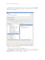
2.3.1 Building the Baseline Programs
We have provided basic makefiles for compiling the baseline programs for each programming
model. You may need to modify these to specify the location of your PPW installation (if
the compiler wrappers are not in your path) or add any necessary compiler options. Running
make for a given programming model should then generate two baseline programs, called
ppw_base_all and ppw_base_a2a.
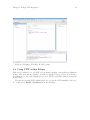
2.3.2 Running the Baseline Programs
The ppw_base_all program needs to be run only with a system size of 2, while the ppw_
base_a2a program should be run with system sizes ranging from 2 to 32. We have provided
basic run.sh scripts (for each programming model) to run the baseline programs using the
appropriate system sizes. You may need to modify the scripts to specify the appropriate
run command(s) for your system. Also, in some cases the scripts may not be useful for
invoking the baseline programs on your system, and you’ll need to manually run the baseline
programs in the appropriate manner.
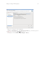
2.3.3 Using the Baseline PAR Files
Once the instrumented baseline programs have been run, you should obtain output PAR files
with specific names: ppw_base_all.par for the ppw_base_all program, and ppw_base_
a2a_N.par files for runs of the ppw_base_a2a program on system size N. These files should
now be transferred to the appropriate location within your frontend PPW installation,
normally the analysis/baseline/PMODEL directory, where PMODEL is UPC, SHMEM, or
MPI. If you use the PPW frontend on a separate workstation from your parallel system,
you will need to use a file transfer program to copy the baseline PAR files to the appropriate
directory within your PPW installation on your workstation.
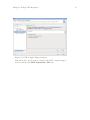
Now when you first run analyses from within the PPW GUI, the baseline PAR files will
be used to generate files containing baseline values for operations in a given programming
model. These resulting files, called ppw_baseline.txt and located within each of the
subdirectories of the analysis/baseline directory of the PPW frontend installation, should
be deleted if you need to regenerate baseline data from new baseline PAR files (for example,
if you are using a different system than before).
Chapter 3: Analyzing UPC Programs
18
3 Analyzing UPC Programs
To analyze the performance of your UPC programs, you will need to configure PPW to use
a UPC compiler. If you haven’t configured PPW to use a UPC compiler yet, please see
Section 2.2 [Backend Installation], page 12.
When measuring performance data for UPC programs, all shared data references occurring through direct variable accesses will be attributed to the ‘upc_get’ and ‘upc_put’
regions. Shared data references with affinity to the current thread will be attributed to
the ‘upc_get_local’ and ‘upc_put_local’ regions. Additionally, in some UPC implementations (including Berkeley UPC), a ‘upc_barrier’ will be split into ‘upc_notify;
upc_wait;’ and show up in the ‘upc_notify’ and ‘upc_wait’ regions.
3.1 Compiling UPC Programs
In order to analyze the performance of your UPC program, you’ll first need to recompile it
using a PPW compiler wrapper script. Instead of compiling with upc or upcc, use ppwupcc
instead.
The ppwupcc wrapper script has a few important options that can reduce the amount of
performance data collected and help reduce instrumentation overhead. In particular, you
can pass the ‘--inst-local’ and ‘--inst-functions’ options to ppwupcc to record more
detailed performance information at the cost of higher perturbation.
We recommend compiling with the --inst-functions flag, which will allow you to
relate performance information back to individual functions. The ‘--inst-local’ option
is useful if you’d like to identify segments of code that frequently access shared data local
to the node, in addition to remote shared data accesses. Local accesses will show up in
visualizations under regions having a ‘local’ suffix, such as ‘upc_get_local’. Note that
tracking shared-local accesses is more expensive than tracking remote accesses only, and
may cause PPW to over-report the actual time taken for parts of your code that perform
many local data accesses in a short amount of time. If you experience very high overhead
(ie, much longer execution times) while running your program under PPW, see Chapter 7
[Managing Overhead], page 26 for tips on how to reduce that overhead.
For more information on the ppwupcc command, please see Section B.9 [ppwupcc],
page 90.
3.2 Running UPC Programs
To run your instrumented application, use the ppwrun command in front of your application’s run command invocation. Note that you must recompile your application first; for
more information please see Section 3.1 [Compiling UPC Programs], page 18.
For instance, if you normally run your application using the following command:
$ upcrun -n 16 ./myapp 1 2 3
you would use this command instead:
$ ppwrun --output=myapp.par upcrun -n 16 ./myapp 1 2 3
For UPC programs, PPW does not currently support noncollective UPC exits, such as
an exit on one thread that causes a SIGKILL signal to be sent to other threads. As an
example, consider the following UPC program:
Chapter 3: Analyzing UPC Programs
19
...
int main() {
if (MYTHREAD) {
upc_barrier;
} else {
exit(0);
}
return 0;
}
In this program, depending on the UPC compiler and runtime system used, PPW may
not write out valid performance data for all threads. A future version of PPW may add
“dump” functionality where complete profile data is flushed to disk every N minutes, which
will allow you to collect partial performance data from a long-running program that happens
to crash a few minutes before it is completed. However, for technical reasons PPW will
generally not be able to recover from situations like these, so please do try to debug any
crashes in your program before analyzing it with PPW.
For more information on the ppwrun command, please see Section B.10 [ppwrun], page 93.
3.3 Recording Phase Data in UPC
While the ‘--inst-local’ and ‘--inst-functions’ instrumentation options provided by
ppwupcc do provide several different options for attributing performance information to specific regions of code in your program, sometimes simply having function-level performance
information does not give you enough information to analyze your program. Rather, it
might be useful to track time spent in a particular phase of your program’s execution.
In the future, PPW may add support to automatically detect program phases based
on an online analysis of barriers. In the meantime, if you’d like to collect performance
information for particular phases of your program’s execution, you’ll need to manually add
calls to PPW’s measurement API in your program.
As an example, suppose you’ve written a UPC program that resembles the following
structure:
#include <upc.h>
int main() {
/* initialization phase */
/* ... */
upc_barrier;
/* computation phase with N iterations */
for (i = 0; i < N; i++) {
/* ... */
upc_barrier;
}
/* communication phase */
/* ... */
Chapter 3: Analyzing UPC Programs
20
upc_barrier;
return 0;
}
and you compile this program with ppwupcc --inst-functions main.upc. When viewing
this performance data, you will get information about how long each thread spent executing ‘main’, but not much information about each of the phases within your program. If
your computation phase has a load-balancing problem, this might be hard to detect just
by examining performance data for ‘main’. Similarly, if you have a complicated program
structure where program phases are not neatly divided into function calls, then you will
have a hard time localizing performance problems to particular phases of your program’s
execution.
Using PPW’s measurement API, you would do this:
#include <upc.h>
#include <pupc.h>
int main() {
unsigned int evin, evcp, evcm;
evin = pupc_create_event("Init phase", NULL);
evcp = pupc_create_event("Compute phase", "%d");
evcm = pupc_create_event("Comm phase", NULL);
/* initialization phase */
pupc_event_start(evin);
/* ... */
upc_barrier;
pupc_event_end(evin);
pupc_event_start(evcp, -1);
/* computation phase with N iterations */
for (i = 0; i < N; i++) {
pupc_event_atomic(evcp, i);
/* ... */
upc_barrier;
}
pupc_event_end(evcp, -1);
/* communication phase */
pupc_event_start(evcm);
/* ... */
upc_barrier;
pupc_event_end(evcm);
return 0;
}
Chapter 3: Analyzing UPC Programs
21
For full details on the UPC measurement API, see Section A.1 [UPC Measurement API],
page 69.
3.4 Further UPC Examples
For more examples showing how to use PPW to analyze UPC applications, please see the
‘share/examples/upc’ directory of your PPW installation.
Chapter 4: Analyzing SHMEM Programs
22
4 Analyzing SHMEM Programs
To analyze the performance of your SHMEM programs, you will need to configure PPW to
use your SHMEM library. If you haven’t configured PPW to use your SHMEM library yet,
please see Section 2.2 [Backend Installation], page 12.
4.1 Compiling SHMEM Programs
In order to analyze the performance of your SHMEM program, you’ll first need to recompile it using a PPW compiler wrapper script. Instead of compiling with cc or gcc, use
ppwshmemcc instead.
For more information on the ppwshmemcc command, please see Section B.7 [ppwshmemcc], page 86. If you experience very high overhead (ie, much longer execution times)
while running your program under PPW, see Chapter 7 [Managing Overhead], page 26 for
tips on how to reduce overhead.
4.2 Running SHMEM Programs
To run your instrumented application, use the ppwrun command in front of your application’s run command invocation. Note that you must recompile your application first; for
more information please see Section 4.1 [Compiling SHMEM Programs], page 22.
For instance, if you normally run your application using the following command:
$ srun -n 16 ./myapp 1 2 3
you would use this command instead:
$ ppwrun --output=myapp.par srun -n 16 ./myapp 1 2 3
For more information on the ppwrun command, please see Section B.10 [ppwrun], page 93.
Note: The current OpenSHMEM support does not profile the following functions:
start pes, my pe, num pes, shmem pe accessible, shmem add accessible, shmem ptr,
shmemalign.
4.3 Recording Phase Data in SHMEM
While the ‘--inst-functions’ instrumentation option provided by ppwshmemcc does provide some flexibility for attributing performance information to specific regions of code in
your program, sometimes simply having function-level performance information does not
give you enough information to analyze your program. Rather, it might be useful to track
time spent in a particular phase of your program’s execution.
If you’d like to collect performance information for particular phases of your program’s
execution, you’ll need to manually add calls to PPW’s measurement API in your program.
For full details on the SHMEM measurement API, see Section A.2 [SHMEM Measurement
API], page 73.
4.4 Further SHMEM Examples
For more examples showing how to use PPW to analyze SHMEM applications, please see
the ‘share/examples/shmem’ directory of your PPW installation.
Chapter 5: Analyzing MPI Programs
23
5 Analyzing MPI Programs
To analyze the performance of your MPI programs, you will need to configure PPW to use
your MPI library. If you haven’t configured PPW to use your MPI library yet, please see
Section 2.2 [Backend Installation], page 12.
5.1 Compiling MPI Programs
In order to analyze the performance of your MPI program, you’ll first need to recompile it
using a PPW compiler wrapper script. Instead of compiling with mpicc, use ppwmpicc.
For more information on the ppwmpicc command, please see Section B.8 [ppwmpicc],
page 88. If you experience very high overhead (ie, much longer execution times) while
running your program under PPW, see Chapter 7 [Managing Overhead], page 26 for tips
on how to reduce overhead.
5.2 Running MPI Programs
To run your instrumented application, use the ppwrun command in front of your application’s run command invocation. Note that you must recompile your application first; for
more information please see Section 5.1 [Compiling MPI Programs], page 23.
For instance, if you normally run your application using the following command:
$ srun -n 16 ./myapp 1 2 3
you would use this command instead:
$ ppwrun --output=myapp.par srun -n 16 ./myapp 1 2 3
For more information on the ppwrun command, please see Section B.10 [ppwrun], page 93.
5.3 Recording Phase Data in MPI
While the ‘--inst-functions’ instrumentation option provided by ppwmpicc does provide
some flexibility for attributing performance information to specific regions of code in your
program, sometimes simply having function-level performance information does not give
you enough information to analyze your program. Rather, it might be useful to track time
spent in a particular phase of your program’s execution.
If you’d like to collect performance information for particular phases of your program’s
execution, you’ll need to manually add calls to PPW’s measurement API in your program.
For full details on the MPI measurement API, see Section A.3 [MPI Measurement API],
page 75.
5.4 Further MPI Examples
For more examples showing how to use PPW to analyze MPI applications, please see the
‘share/examples/mpi’ directory of your PPW installation.
Chapter 6: Analyzing C Programs
24
6 Analyzing C Programs
While PPW was designed to work best with parallel programs, you can still use it to analyze
the performance of sequential C applications. For best results, you should install a UPC
compiler with GASP support (such as Berkeley UPC) and configure PPW to use that UPC
compiler. See Section 2.2 [Backend Installation], page 12.
6.1 Compiling C Programs
In order to analyze the performance of your sequential C program, you’ll first need to
recompile it using one of the PPW compiler wrapper scripts. Simply use the wrapper
scripts in place of your normal C compiler (eg, in place of gcc).
For sequential C programs, you have two options:
• Compile with ppwupcc: Since every C program is a valid UPC program, you should
be able to compile your application with a UPC compiler. See Section 3.1 [Compiling
UPC Programs], page 18.
• Compile with ppwcc: If compiling your C application with a UPC compiler is not
a viable option, you can still use PPW with your sequential code if you manually
instrument your code with API calls. See Section 6.3 [Recording Phase Data in C],
page 24.
For more information on the compiler wrapper commands, please see Section B.6 [ppwcc],
page 84, or Section B.9 [ppwupcc], page 90 if you are using a UPC compiler installation.
If you experience very high overhead (ie, much longer execution times) while running your
program under PPW, see Chapter 7 [Managing Overhead], page 26 for tips on how to reduce
overhead.
6.2 Running C Programs
To run your instrumented application, use the ppwrun command in front of your application’s run command invocation. Note that you must recompile your application first; for
more information please see Section 6.1 [Compiling C Programs], page 24.
For instance, if you normally run your application using the following command:
$ ./myapp 1 2 3
you would use this command instead:
$ ppwrun --output=myapp.par ./myapp 1 2 3
For more information on the ppwrun command, please see Section B.10 [ppwrun], page 93.
6.3 Recording Phase Data in C
While the ‘--inst-functions’ instrumentation option provided by ppwupcc and ppwcc
does provide some flexibility for attributing performance information to specific regions
of code in your program, sometimes simply having function-level performance information
does not give you enough information to analyze your program. Rather, it might be useful
to track time spent in a particular phase of your program’s execution.
If you’d like to collect performance information for particular phases of your program’s
execution, you’ll need to manually add calls to PPW’s measurement API in your program.
For full details on the C measurement API, see Section A.4 [C Measurement API], page 76.
Chapter 6: Analyzing C Programs
25
6.4 Further C Examples
For more examples showing how to use PPW to analyze C applications, please see the
‘share/examples/sequential’ directory of your PPW installation.
Chapter 7: Managing Measurement Overhead
26
7 Managing Measurement Overhead
The simplest way to reduce the overhead caused by PPW is try compiling your program
without using the ‘--inst-functions’ or ‘--inst-local’ compilation flags. If this does
not solve your problem, or if it eliminates too much useful performance information, read
on.
Aside from the compilation flags mentioned above, PPW provides two methods of controlling overhead in your program: selective instrumentation, and selective measurement.
7.1 Selective Instrumentation
The most effective way of removing overhead caused by PPW is to simply avoid instrumentation of parts of your program that generate a lot of overhead. If you have a function in
UPC that looks similar to the following:
int argplusfive(int arg) {
return arg + 5;
}
then you will undoubtedly experience a large amount of overhead if you compile your code
with the ‘--inst-functions’ flag, especially if you call ‘argplusfive’ frequently in a short
period of time.
In such cases, you might not be interested in the time taken for each and every call to
‘argplusfive’ since you know it is not a likely source of performance problems. If so, you
can use the ‘pupc’ pragmas defined in the GASP specification to ask the compiler to inhibit
instrumentation around lexically-scoped regions of code. For instance, you might do the
following:
#pragma pupc off
int argplusfive(int arg) {
return arg + 5;
}
#pragma pupc on
For most compilers, this should prevent PPW from receiving performance information
about the ‘argplusfive’ function at runtime. However, if your GASP-aware compiler
instruments at function callsites instead of function definitions, then you’ll have to move
the ‘#pragma pupc’s to surround the location of each callsite to ‘argplusfive’. For the
current generation of UPC GASP-aware compilers supporting function call instrumentation
(Berkeley UPC and GCC UPC), you will need to use the ‘#pragma pupc’s around function
definitions and not callsites.
As an interesting side note, if you do experience a high amount of overhead due to
frequent calls to short-lived functions, you might consider inlining those function calls via
macros or compiler directives/keywords such as ‘inline’. Function calls can add quite a bit
of overhead if your function bodies consist of a small amount of instructions, so you might
see a big performance increase by playing around with your compiler’s inlining settings.
In addition to the line-level ‘#pramga pupc’ instrumentation controls, you may also give
the ‘--noinst’ flag to PPW’s compiler wrapper scripts to disable instrumentation for whole
files. This can be useful for ignoring parts of your application that have already been tuned
or that are not important to overall performance.
Chapter 7: Managing Measurement Overhead
27
The C and SHMEM API provides similar pragmas (‘#pragma cprof’ and ‘#pragma
pshmem’, respectively) to control instrumentation for particular regions of code.
7.2 Selective Measurement
PPW also supports a simple API for turning measurement on and off for particular parts
of your program code. This API does not affect the instrumentation process, so it is not
as effective of an overhead reduction technique as the techniques described in Section 7.1
[Selective Instrumentation], page 26. However, since the technique is API-based, it does
offer a lot of flexibility.
Listed below is a quick example of how to use the UPC measurement controls:
#include <upc.h>
#include <pupc.h>
int main() {
/* turn off measurement for initialization process */
pupc_control(0);
do_init();
/* now record data about computation... */
pupc_control(1);
do_computation();
/* ignore data collection and presentation phase */
pupc_control(0);
do_process_results();
/* finally, turn control back on to dump out performance data */
pupc_control(1);
return 0;
}
Since the GASP ‘pupc’ functions are not part of the UPC specification, you’ll probably
want to protect any code that uses these functions with an ‘#ifdef __UPC_PUPC__’. For
example, you could do something like this:
#ifdef __UPC_PUPC__
#define PUPC_CONT(a) pupc_control(a)
#else
#define PUPC_CONT(a)
#endif
and use the ‘PUPC_CONT’ macro in place of ‘pupc_control’ function calls. That way, your
program code still compiles on systems without GASP support.
It is important to keep in mind that the ‘pupc_control’ function does not change the
instrumentation code added to your program in any way; rather, it tells PPW to ignore
performance information for parts of your program’s execution.
The C and SHMEM API provides similar functions (‘cprof_control’ and
‘pshmem_control’, respectively) to control measurement for particular regions of code. See
Appendix A [API Reference], page 69 for more details on the measurement API provided
by PPW.
Chapter 7: Managing Measurement Overhead
28
7.3 Using Selective File
This feature is currently available only to UPC.
It is also possible to provide a selective file to ppw by passing an option
‘--selective-file=file’ to Section B.10 [ppwrun], page 93. The file specifies the list of
events that should be excluded from measurment and a list of events that should never be
throttled. An example selective file is shown below,
#list of events to exclude
EXCLUDE_START
ft.c:fftz2
input.c:*
*:upc_notify
EXCLUDE_END
#list of events not to throttle
INCLUDE_START
ft.c:cfftz
INCLUDE_END
Each line can contain only one of the following:
• Defination of an event e.g:ft.c:cfftz
• Predefined string e.g: INCLUDE END
• Comment: line with ’#’ as first charecter. Please note, there cannot be a comment
and any of the above on same line
Each event is specified as FileName:EventName. Either FileName or EventName can
be * which means all the files or all the events. Formations using wild-card charecters
(e.g: ft*.c, upc * lock, ft?.upc) are not supported in-order to keep the run time overhead
due to selective measurment low. Only the basename of the specified FileName would be
considered. For example if the specified filename is /usr/local/hello.c only hello.c will be
considered.
All events that should be exclude should be defined between EXCLUDE START and
EXCLUDE END and all events that should be included shoucl be defined between INCLUDE START and INCLUDE END.
7.4 Throttling
Throttling is a technique where measurment of certain events will be stopped if it crosses
certain predefined thresholds. In the current implementation we throttle only user-level
events (function calls) and we consider two different threshold for throttling:
• ‘throttling-count’ Number of times an event is invoked
• ‘throttling-duration’ Average duration of an event
An event will be throttled (or won’t be measured any further) during runtime, if it was
invoked more than ‘throttling-count’ and the average duration for that event was less
than ‘throttling-duration’. The events specified in selective file will not be considered
for throttling.
Chapter 7: Managing Measurement Overhead
29
If a user function func1 is throttled, then it will appear as func1(throttled) in the performance data.
Throttling is enabled by default and can be disabled by passing ‘--disable-throttling’
to Section B.10 [ppwrun], page 93.
The thresholds can be modified by passing
‘--throttling-count=COUNT’ and ‘--throttling-duration=DURATION’ to Section B.10
[ppwrun], page 93.
Chapter 8: Frontend GUI Reference
30
8 Frontend GUI Reference
As described in the “Frontend Installation” portion of the PPW manual (Section 2.1 [Frontend Installation], page 12), PPW provides a Java-based graphical user interface (GUI) for
browsing your application’s performance data. We describe this interface in this part of the
manual.
8.1 Overview of the PPW GUI
The GUI provided by PPW allows you to view the performance data obtained during the
measurement process.
Figure 8.1: Default PPW GUI
See Figure 8.1 for a screenshot of this interface as it appears when no data file is loaded.
PPW’s user interface is grouped into four main sections: the open file list (upper left),
the experiment information panel (lower left), the source panel (lower right, not shown),
and the visualization panel (upper right).
8.1.1 Open File List
The open file list shows all currently-open files. Some visualizations deal with experiment
data from more than one run, so PPW allows you to open and browse performance data
for more than one data file.
PPW also allows you to organize your data files into revisions, which you can think of as
a particular “version” of your program. For instance, you might have two possible methods
of runtime load-balancing strategies and you want to use PPW to compare the performance
Chapter 8: Frontend GUI Reference
31
of both strategies side-by-side. In this case, you’d create two revisions, and load up different
performance data sets corresponding to different system sizes into each revision. Revisions
can also be used to compare the performance of a program across different architectures,
communication hardware, etc.
PPW’s visualizations are designed to treat data files within a particular revision as data
from the same revision run on different number of nodes. If you don’t follow this convention
when loading in data files, some of the visualizations dealing with more than one data file
will show strange results. However, if you are simply using visualizations that display data
for a single file only (such as the Tree Table and Data Transfers visualizations) you do not
need to load data files in any special way.
To create or modify revisions in the PPW GUI, choose File > New revision..., File >
Rename revision..., or File > Close revision... from the menu bar. To load data files into
a particular revision, select a revision by clicking on that revision name (ie, click “Default
Revision” in Figure 8.1) or left-click on a file within that revision, then choose File > Open...
from the menu bar. Additionally, you may right-click on a revision name in the open file
list to add files to that revision. Files can also be dragged with the mouse from one revision
to another, or dragged from outside the PPW program into the file list and opened in the
current revision.
Figure 8.2: Revisions Example
As a concrete example, assume you have two strategies for performing calculating the
value of Pi, “Strategy A” and “Strategy B”, and you have data sets for both of these
methods with runs of size one, eight, and sixteen nodes. In this case you’d want to create
revisions as shown in Figure 8.2.
Chapter 8: Frontend GUI Reference
32
For complex analyses and programs with many different revisions, it might take a while
to set up your revision sets just the way you want them. To save time, PPW allows you to
save and restore the current workspace (which includes all revisions and files within those
revisions) if you want to come back to the same revision set up later on. To save the current
set of loaded files, choose File > Workspace > Save workspace from the menu bar and give
your saved file an extension of ‘.pbw’. To restore a previously-saved set of loaded files,
choose File > Workspace > Load workspace from the menu bar and select a file you have
previosly saved.
Note: The workspace files you save use absolute paths, which means they will
not work on another machine unless the data files reside in the same location
on that machine too.
8.1.2 Experiment Information Panel
The information panel in the lower left of the PPW GUI shows basic data about the
currently-selected data file, including the date the data was gathered, the number of threads
in the run, if the data file contains trace records, and the date the executable for this program
was built.
To get more detailed information about a particular data file, choose File > Experiment
info from the menu bar. PPW tracks a lot of information about your program, including:
• information about when the program was built and run
• the commandline arguments given to the program
• a snapshot of all environment variables in effect when the program was run
• a list of hostnames for each node the program was run on
• all the “ident” strings in your program’s executable
In particular, the “ident” strings for your program’s executable will contain a lot of useful
(but detailed) information, especially if you use Berekley UPC and/or Quadrics network
hardware.
8.1.3 Source Panel
The source panel shows a snapshot of source code that was used to generate the performance
data shown by each visualization. If you notice source code files missing from your data set,
see the notes section for Section B.6 [ppwcc], page 84, Section B.7 [ppwshmemcc], page 86,
and Section B.9 [ppwupcc], page 90.
8.1.4 Visualization Panel
The visualization panel shows a tabbed interface of available visualizations. To switch to a
different visualization, click on the visualization’s name in tab list.
Most visualizations will show performance data for the currently-selected file in the open
file list. To change the currently-selected file, left-click on a file within the open file list on
the left side of the screen. For visualizations that work on a group of files in a single revision,
you may change which revision is used to display data by left-clicking on the revision name
in the open file list.
The available visualizations are:
• Profile table (see Section 8.2 [Profile Table], page 33)
Chapter 8: Frontend GUI Reference
•
•
•
•
33
Tree table (see Section 8.3 [Tree Table], page 34)
Data transfers (see Section 8.4 [Data Transfers], page 35)
Array distribution (see Section 8.5 [Array Distribution], page 37)
Profile charts (see Section 8.6 [Profile Charts], page 38)
Each of these visualizations is discussed in the following sections.
8.2 The Profile Table Visualization
The profile table visualization provides a tabular view of statistical profile data for all regions
of a program. The table shows data for one metric at a time, with ‘Time’ being the default
metric to show. The data is either for a single thread or for ‘All Threads’, as selected
using the Thread drop-down box. If ‘All Threads’ is selected, then the current aggregation
method as specified in the Options > Aggregation Method menu is used to aggregate the data
across all threads. To see how metric values for a particular region of code are distributed
across all threads, double-click on that region to bring up a graph illustrating the breakdown
of the selected region across all nodes in the run.
Figure 8.3: Profile table visualization
See Figure 8.3 for a screenshot of the profile table visualization.
The following columns are used to show the profile data:
‘Name’
the name of the region (often the name of a function)
‘Callsite’
the line of code the region was called from, or the line of code where the region
was defined if the actual callsite is not available
Chapter 8: Frontend GUI Reference
‘Total’
the total value of the metric for the region, inclusive of subregions
‘Self’
the value of the metric for this region alone, exclusive of subregions
‘Min’
the minimum value of the metric across all instances of this region
‘Max’
the maximum value of the metric across all instances of this region
‘Calls’
how many times this region was called
34
‘Sub Calls’
how many subregions this region called
If a region has multiple callsites, PPW may group these together if the callsites can be
grouped together without affecting the interpretation of the performance data. By clicking
on the tree controls in the first column of a grouped entry (which will have no entry in the
‘Callsite’ column), you can hide or show the callsites that were grouped together for that
particular region. Entries in the table corresponding to a single callsite will have a right
arrow icon next to their region name, while grouped entities will show a circular icon. For
example, in Figure 8.3, PPW has grouped all calls to ‘upc_notify’ underneath a single
generic ‘upc_notify’ entry.
Right-clicking on any column header will bring up a menu allowing you choose which
columns from among those listed above you would like to see in the table. By default, only
a few columns are shown.
Each entry in the profile table is coded with a color to describe the class the entry falls
into. The colors used are:
Black
a user region, such as a function call or (eg, ‘main’)
Blue
a language region, such as a barrier (eg, ‘upc_barrier’)
Red
a region that may have its time values over-reported time due to overheads
caused by PPW’s measurement code
If a particular region is flagged in red, that means the average time taken to execute
this region is low enough that tracking performance information for each call to this region
might add too much overhead to give you an accurate idea of this function’s effect on overall
execution time. In other words, PPW might be overestimating the actual time taken for this
region in an unprofiled run. Future versions of PPW may include an overhead compensation
feature that attempts to compensate for any perturbations caused by executing PPW’s own
measurement code.
If you find that PPW severely perturbs your application’s performance characteristics,
please see Chapter 7 [Managing Overhead], page 26 for tips on how to reduce PPW’s
performance footprint.
8.3 The Tree Table Visualization
The tree table is like the profile table in that it shows a tabular view of profile data.
However, instead of just showing a flat list of regions in your program, the tree table shows
you performance information in relation to your application’s call paths. Related callsites
for a region are still grouped together, but only if the callsites occurred within the same
call path.
Chapter 8: Frontend GUI Reference
35
Figure 8.4: Tree table visualization
See Figure 8.4 for a screenshot of the tree table visualization.
The tree table visualization has the same display characteristics and behaviors as the
profile table, including color coding of regions, double-clicking to view region breakdowns
across all nodes, and the ability to hide and show each column. For more information about
these features, see Section 8.2 [Profile Table], page 33.
8.4 The Data Transfers Visualization
This visualization provides a graphical view of the data transfers that took place during
the execution of the user program. Note that in order to view data transfer statistics, you
must use ppwrun’s ‘--comm-stats’ option when launching your application.
Chapter 8: Frontend GUI Reference
36
Figure 8.5: Data transfers visualization
See Figure 8.5 for a screenshot of the data transfers visualization.
The data-transfer information is shown in a grid, with each cell in the grid containing the
data-transfer value of the current metric for a particular initiating thread and data affinity
thread. Here the initiating thread is the thread which invoked the data-transfer operation,
and the data affinity thread is the thread where the data resided.
The value for a given cell is represented using a color-coding scheme. The legend near
the right side of the window shows the mapping between colors and metric values, with the
maximum value corresponding to red and the minimum value to purple.
Controls near the top of the window allow you to specify the visualization’s content and
appearance. The Zoom Level control allows you to adjust the zoom level to increase or
decrease the number of cells show on the screen at once.
The Metric drop-down box lets you select from the following data-transfer metrics:
‘Bytes’
The amount of data transferred, in bytes
‘Comm Operations’
The number of data-transfer operations
‘Avg Payload Size’
The average size of the data-transfer payload
The Operation drop-down box lets you choose whether to show the metric for only
‘Puts’, for only ‘Gets’, or for ‘Puts + Gets’. By default, ‘Puts + Gets’ is selected.
Finally, the Payload Size drop-down box allows you to choose a payload size range for
which to show data-transfer data.
Chapter 8: Frontend GUI Reference
37
The data transfers visualization is helpful in identifying problems associated with the
communication pattern in your program. Threads that initiate an inordinate amount of
communication will have their corresponding row in the grid stand out in red. Similarly,
threads which have affinity to data which is transferred a lot will have their column in the
grid stand out.
8.5 The Array Distribution Visualization
This visualization shows how each statically-allocated shared array was distributed across
threads at runtime, and is only relevant for UPC programs.
Figure 8.6: Array distribution visualization
See Figure 8.6 for a screenshot of the array distribution visualization.
The Array drop-down box allows you to select an array from the data file of your program. Based on the original declaration of this selected array, the Blocksize and Dimensions
fields will be filled in. Additionally, the Threads field is automatically set to the number of
threads with which the program was executed. This information is then used to graphically
show how the array is distributed among the threads as dictated by the UPC language
specification.
In this graphical view, the color of a particular cell is mapped to the array indices of
the element that cell represents, with black mapped to 0 and bright green mapped to the
maximum value of that array index.
The Blocksize, Dimensions, and Threads fields can all be modified to allow you to see
how a different distribution of an array would appear. You may use arbitrary expressions
Chapter 8: Frontend GUI Reference
38
involving THREADS in each of the fields, although remember to put brackets around each
dimenion in the Dimensions field as you would if you were declaring it in your source code.
8.6 The Profile Charts Visualization
This visualization provides a number of charts showing various graphical depictions of statistical profile data. These charts include the following:
• Operation Types Pie Chart
• Profile Metrics Pie Chart
• Profile Metrics Bar Chart
• Thread Breakdown Line Chart
• Total Times Line Chart
• Total Times by Function Bar Chart
For each of the charts, right-clicking the chart will bring up a menu allowing you to
perform several operations on the chart, such as adjusting the display properties, saving it
to an image file, or adjusting the zoom level.
Some of the charts deal with displaying information for regions of code. In cases where
different callsites for a particular region can’t be safely aggregated together (eg, nested
‘upc_forall’ loops), callsite information will be attached to the region name.
8.6.1 Operation Types Pie Chart
This chart is a pie chart that shows how much time your application spent doing different
types of operations, such as time spent in locks, gets, or barriers.
Figure 8.7: Operation types pie chart
Chapter 8: Frontend GUI Reference
39
See Figure 8.7 for a screenshot of this pie chart.
This pie chart gives you a very high-level view how time is spent in your program. It
can be useful for determining if your application is compute-bound, throughput-bound, or
has excessive calls to synchronization operations.
8.6.2 Profile Metrics Pie Chart
This chart shows profile metrics in the form of a pie chart, where each slice of the pie
represents self time for one region of your program. Slices are included for the ten regions
with the highest self times; the ‘Other’ region includes all other regions that do not fall in
the top ten.
Figure 8.8: Profile metrics pie chart
See Figure 8.8 for a screenshot of this pie chart.
Since this chart is based on self (exclusive) time, it helps you see the breakdown of the
most costly individual regions of code where time spent can be attributed to that region
alone. This can help you identify computationally-intensive region of code, such as poorlytuned computation kernels.
8.6.3 Profile Metrics Bar Chart
This chart is a bar chart in which the bars depict the total time spent in a given region of
the user program. One bar is shown for each of the top ten regions in your program (sorted
by total time).
Chapter 8: Frontend GUI Reference
40
Figure 8.9: Profile metrics bar chart
See Figure 8.9 for a screenshot of this bar chart.
This chart helps you quickly pick out which regions are taking the most time in your
program, so you can decide where to focus your efforts in optimizing particular regions. It
also gives a visual indication of the relationship between different regions in your program,
in terms of how much total time they take.
8.6.4 Thread Breakdown Line Chart
This chart shows a breakdown of the total time spent in a given region across the various
threads in the system. The Region drop-down box near the top-right of the window allows
you to select the region for which the chart is shown.
Chapter 8: Frontend GUI Reference
41
Figure 8.10: Thread breakdown line chart
See Figure 8.10 for a screenshot of this chart.
This chart can be useful in identifying any load-balancing issues in your program. In
a perfectly well balanced program, the time spent in a given region will be the same on
each of the threads in the system. Thus, if you observe that one or more of the threads is
spending significantly more or less time in a particular region than the other threads, you
should investigate further to determine if this is the result of a load-balancing problem in
you program.
8.6.5 Total Times Line Chart
This chart allows you to compare different runs of your program across different revisions
using different numbers of nodes.
In this chart, each line corresponds to a revision created in the open files list. Points for
each line are obtained by plotting the number of nodes versus total execution time for each
data file listed in a particular program revision. In other words, what you are looking at
here is the classic time vs. nodes speedup chart.
Chapter 8: Frontend GUI Reference
42
Figure 8.11: Total times line chart (summing aggregation)
See Figure 8.11 for a screenshot of this chart.
It is important to note that this chart is affected by the aggregation method option
(Options -> Aggregation method from the menu bar). If you are using the default “summing”
aggregation method in which displayed times are really a sum of all times taken across every
node, then you would expect to have a perfectly straight line. For example, if your program
had 100% efficiency and you ran your program on four nodes, then running it eight nodes
should take half as long. However, since there are twice as many nodes, the sum of execution
times across all nodes will be the same.
Therefore, to interpret the previous screenshot (see Figure 8.11), we see that the program does not have perfectly-linear speedups because the lines are not perfectly straight.
Additionally, the big jumps between one and eight nodes of the “Orig” and “Orig.opt”
revisions tell us there is a big drop in efficiency when moving beyond one node, but the
efficiency doesn’t seem to get worse as we increase the number of nodes. If we compare
these lines to the “Fixed” and “Fixed.opt” lines, we see that these revisions do not exhibit
the same efficiency drop as we move beyond one node, so whatever changes we made to
those revisions has nearly eliminated the efficiency problem.
Chapter 8: Frontend GUI Reference
43
Figure 8.12: Total times line chart (average aggregation)
If you are using one of the non-default aggregation methods such as min, max, or average,
then you will end up with a more traditional type of time vs. nodes chart. See Figure 8.12
for an example of the same data set from Figure 8.11 using the average aggregation method
instead of the summing aggregation method.
For more information on how to set up program revisions, see Section 8.1 [GUI Overview],
page 30.
8.6.6 Total Times by Function
This chart allows you to compare runs of a particular revision of your program on different
system sizes, illustrating how time is spent in the various regions (functions) of a program
revision across different system sizes. This chart is similar to the previous chart, except that
it shows a breakdown of time for regions within a program revision rather than time spent
across all revisions. In essence, this chart “blows up” one particular line from the Total
Times Line Chart and shows the breakdown of time for each run across different regions in
your program.
Chapter 8: Frontend GUI Reference
44
Figure 8.13: Total times by function (summing aggregation)
See Figure 8.13 for an example screenshot of this chart.
As with the previous chart, this chart is affected by the aggregation method option
(Options -> Aggregation method from the menu bar). If we are using the default “summing”
aggregation, then we’d expect a perfectly-horizontal line as we increase the number of nodes.
See the notes on the Program Speedup Line Chart for more information.
To interpret the screenshot in Figure 8.13, we see that the “Orig” revision of the program
we’re analyzing has a clear scalability problem when moving beyond one node. In particular,
the time taken for the ‘upc_lock’ and ‘upc_notify’ regions (which are parts of UPC’s
barrier and lock language constructs) greatly jump once moving past one node, but the
percentage of time taken for that lock operation decreases as the percentage of the barrier
operation increases when increasing the number of nodes in the run. From this graph, we
can determine that our example program has a lock contention issue that may be resuling
in extra time spent in a barrier construct.
Chapter 8: Frontend GUI Reference
45
Figure 8.14: Total times by function (average aggregation)
If you are using one of the non-default aggregation methods such as min, max, or average,
then you will end up with a chart that is slightly harder to interpret and make good
use of. See Figure 8.14 for an example of the same data set from Figure 8.13 using the
average aggregation method instead of the summing aggregation method. For this chart,
we recommend sticking with the summing aggregation method, although flipping between
the min and max aggregation methods may shed some insight into where efficiency losses
are coming from.
For more information on how to set up program revisions, see Section 8.1 [GUI Overview],
page 30.
8.7 Analysis Menu
This section describes the analysis features offered by the PPW GUI, which can be accessed
through the Analysis menu of the GUI.
8.7.1 Application Analysis
PPW provides substantial application-level analysis functionality. The tool uses profile
and/or trace data to automatically identify problem areas, or bottlenecks, within your
application code. Application analysis is initiated by choosing Analysis > Run Application
Analysis from the menu bar in the main PPW GUI. Choosing this menu option brings up
a dialog for specifying various parameters to the application analysis process.
Within the Application Analysis dialog, the Do Filtering option specifies that high-level
profile data should be used for filtering prior to the (potentially time-consuming) bottleneck
Chapter 8: Frontend GUI Reference
46
identification steps. Choosing the Do Trace and Profile Analysis option indicates that both
profile- and trace-based analysis should be performed. Trace-based analysis uses trace
records to identify bottlenecks at a much greater level of detail, but also takes much longer
and of course requires trace records to be present.
Another important option to be aware of is the Number of Analysis Threads. This
specifies how many threads (units of execution on the computer running PPW) should
be used to perform the analysis processing. This value is important for optimizing the
performance of the analysis process. The field will be filled in with a guess of how many
“processors” (or cores) your machine has. This should be a reasonable number of analysis
threads to use, but you may want to adjust the value based on specific knowledge of your
system. For example, if you know your system actually has more processors or otherwise
supports more parallel units of execution, increasing the number of analysis threads may
improve performance. Similarly, if you know you actually have fewer processors available,
or will be utilizing CPU resources for other applications, decreasing the number of analysis
threads may be advisable.
Click Run to start the analysis process. A dialog will appear with a progress bar indicating the status of the processing. Once the process is complete, analysis visualizations
will become available within the PPW GUI.
8.7.2 Scalability Analysis
Scalability analysis is initiated by choosing Analysis > Run Scalability Analysis from the
menu bar in the main PPW GUI. There are currently no parameters to the scalability
analysis processing, so the analysis should begin immediately. After it completes, scalabilityrelated analysis visualizations will become available within the PPW interface.
8.7.3 Memory Leak Analysis
Memory leak analysis is initiated by choosing Analysis > Run Memory Leak Analysis from
the menu bar in the main PPW GUI. For UPC programs the analysis should begin. After
it completes, memory leak analysis visualizations will become available within the PPW
interface.
8.7.4 Saving Analysis Data
After one or more analyses have been run, the resulting analysis data can be saved to
the currently opened PAR file using the Analysis > Save analysis data to current PAR file
option in PPW’s menu bar. Alternatively, a new PAR file containing the analysis data can
be saved by choosing the Analysis > Save new PAR file with analysis data... option. This
will bring up a dialog allowing you to specify the name and location of the file to save.
8.7.5 Load-Balancing Analysis
The load-balancing analysis is accessed by choosing Analysis > Other Analyses > Loadbalancing analysis from the menu bar in the main PPW GUI. Choosing this menu option
brings up a dialog that describes this analysis. By clicking the ‘Next’ button, PPW will
analyze the profile data for the currently-open file. After a short delay, the dialog will
change to show you a list of lines of code with a load-balancing problem.
Chapter 8: Frontend GUI Reference
47
Figure 8.15: Load-balancing analysis
See Figure 8.15 for an example of how the interface looks after running the load-balancing
analysis.
Clicking on each of the entries in the list below will change the graph in the top half of
the screen, showing you the breakdown of time spent on that particular line of code across
all nodes on which the program was run.
The load-balancing analysis uses a very simple method for detecting load-balancing
problems across your application. The analysis uses the heuristic that the sum of time
spent executing each line of profiled code (such as calls to UPC library functions, or lines
of code incurring communication in UPC) should take roughly the same amount of time on
each node in the system. The analysis examines profile data for each profiled line of code,
and flags any line of code where one node’s time differs by more than 25 percent than the
average time taken by all the nodes. After the analysis is finished running, it displays all
flagged source lines, sorted by the greatest difference of time from the average (the ‘Max
imbalance’ column) and shows the sum of differences of each node from the mean in the
‘Total’ column.
In the example screenshot above, line number 860 of ‘CAMEL_upc.c’ had a max imbalance
of 0.95 seconds, meaning that one node’s sum of execution time for line 860 differed from
the mean time across all nodes by 0.95 seconds. By examining the top of the screen we see
that node five is the culprit. The ‘upc_notify’ line in this example belongs to a barrier
synchronization construct; thus, the graph tells us that most nodes end up waiting in a
barrier for node five to catch up to them. This clearly shows the example program has
Chapter 8: Frontend GUI Reference
48
load-balancing problems (node five is a slowpoke!), and that by fixing the imbalance on line
860, we could increase this example application’s efficiency.
The load-balancing analysis can be even more useful when combined with program phase
information recorded using the measurement API described later in the manual. For details on how to use PPW’s measurement API to record application-specific performance
information, see Appendix A [API Reference], page 69.
8.8 Analysis Visualizations
PPW provides a number of visualizations that show the results of the various analyses
offered by the tool. Within the Analysis visualization tab in the PPW GUI, the following
are available:
• High Level Application Analysis
• Experiment Set Analysis
• Analysis Table
• Analysis Summary
Each of these is described in more detail in its corresponding subsection of the manual.
8.8.1 High Level Application Analysis
The High Level Application Analysis visualization shows a high-level breakdown of where
time is spent in your application. Operations performed by the application are placed into
several categories, including computation, global synchronization, point-to-point synchronization, outbound data transfers (sends or puts), and inbound data transfers (receives or
gets).
Chapter 8: Frontend GUI Reference
49
Figure 8.16: High Level Application Analysis visualization
See Figure 8.16 for an example screenshot of this visualization.
The visualization employs a stacked bar chart to show the time breakdown for each node,
which is depicted using a color-coding scheme that assigns colors to each of the available
categories mentioned above. A tab near the top of the display allows you to switch between
Percentages and Times for the operation breakdowns. The Arrange By:, Show Sorted, and
Order: controls let you change the arrangement and ordering of the display.
Left-clicking on a region in the bar chart will bring up a dialog showing detailed information for the corresponding category. Also, if you right-click on the chart, a pop-up menu
with various options will appear.
8.8.2 Experiment Set Analysis
The Experiment Set Analysis visualization shows the results of scalability analysis by plotting the calculated scaling factor value for each experiment within the current experiment
set against the ideal scaling value.
Chapter 8: Frontend GUI Reference
50
Figure 8.17: Experiment Set Analysis visualization
See Figure 8.17 for an example screenshot of this visualization.
Within this visualization the blue line represents the ideal expected scaling, while the
red line shows the observed scaling.
8.8.3 Analysis Table
The Analysis Table visualization can be considered the most important view of analysis
results. The display is broken down into two tables, along with source code shown below.
Chapter 8: Frontend GUI Reference
51
Figure 8.18: Analysis Table visualization
See Figure 8.17 for an example screenshot of this visualization.
The upper table contains profile analysis entries, which are the results of the profile
analysis process. Each of these entries corresponds to a single potential problem location,
as identified using either baseline or deviation comparison. For each of these entries, the
table contains the name of the operation associated with the entry, the operation’s type,
the callsite where operation appeared, the various time values for the entry, and the number
of associated trace analysis entries. Left-clicking on an entry in the table causes the lower
table to show any trace analysis entries associated with that profile analysis entry.
When available, trace analysis entries corresponding to the currently selected profile
analysis entry (in the table above) are shown in the lower table of the Analysis Table
visualization. These entries are the results of detailed analysis using trace records and
basically correspond to individual bottlenecks that occurred in the application. For each of
these, we show the start time, end time, and duration of the bottleneck event, the matching
thread and callsite with which it is associated, and a description of the pattern of the
bottleneck.
8.8.4 Analysis Summary
The Analysis Summary visualization provides a high-level summary of analysis results in a
simple textual form. This includes basic information on whether or certain kinds of analysis
data are available, along with a listing of profile analysis entries for each program thread.
8.9 Jumpshot Introduction
Jumpshot is an open-source timeline viewer that has been bundled with PPW. Jumpshot
does have its own user manual; however Jumpshot is a complex program, and the existing
Chapter 8: Frontend GUI Reference
52
manual is not very user-centric. The rest of this section provides a gentle introduction on
how to use Jumpshot to browse trace data generated by PPW.
8.9.1 Generating Trace Files
In order to view trace data with Jumpshot, you must first generate trace data with PPW.
You’ll have to recompile and re-run your application as described in the previous parts of
this manual. When running your application, use the ‘--trace’ option with the ‘ppwrun’
command. A quick example for a UPC program:
$ ppwupcc -o test test.upc
$ ppwrun --trace --output=mytrace.par srun -N 64 ./test
Once you have generated the trace data, you’ll need to convert it to the SLOG2 file
format that Jumpshot can read. To do this, you can either transfer the ‘mytrace.par’
file to your local workstation and convert the file using PPW’s GUI, or you can try the
conversion on your parallel machine using the par2slog2 command. A quick example of
the par2slog2 command:
$ par2slog2 mytrace.par mytrace.slog2
Converting to SLOG-2
0% done (2 / 58522)
8% done (5000 / 58522) 11.615s left
17% done (10000 / 58522) 8.675s left
25% done (15000 / 58522) 6.087s left
34% done (20000 / 58522) 4.293s left
42% done (25000 / 58522) 3.256s left
51% done (30000 / 58522) 2.716s left
59% done (35000 / 58522) 2.051s left
68% done (40000 / 58522) 1.462s left
76% done (45000 / 58522) 1.005s left
85% done (50000 / 58522) 0.585s left
93% done (55000 / 58522) 0.255s left
SLOG-2 Header:
version = SLOG 2.0.6
NumOfChildrenPerNode = 2
TreeLeafByteSize = 65536
MaxTreeDepth = 6
MaxBufferByteSize = 176385
Categories is FBinfo(610 8960460)
MethodDefs is FBinfo(0 0)
LineIDMaps is FBinfo(292 8961070)
TreeRoot
is FBinfo(175665 8784795)
TreeDir
is FBinfo(3438 8961362)
Annotations is FBinfo(0 0)
Postamble
is FBinfo(0 0)
Finished in 3.591s
Chapter 8: Frontend GUI Reference
53
To do the same conversion on your workstation using the PPW GUI, open up the
‘mytrace.par’ data file with the GUI and choose File > Export > SLOG-2 from the menu
bar.
For best results, we recommend that you do not compile your application with the
‘--inst-functions’ flag as it will generate a lot of extra information that may be overwhelming when displayed with Jumpshot.
The trace data collection and merge process is very expensive when compared with
PPW’s usual profile mode. While eliminating all tracing overhead is usually not possible,
refer to Chapter 7 [Managing Overhead], page 26 for tips on how to reduce this overhead.
8.9.2 Starting Jumpshot
To start Jumpshot, look for a Jumpshot launcher on your workstation near the launcher
you normally use for the PPW GUI. For Windows-based workstations, this is generally
in the Start Menu listed underneath Program Files > PPW. For Mac OSX-based workstations, you’ll want to run the Jumpshot program included in the OSX disk image you
downloaded earlier when installing the frontend. For all other systems, you’ll want to run
the ppwjumpshot command.
For performance reasons, we highly recommend running Jumpshot on your local workstation. Running Jumpshot using a remote X display can be a painfully slow, even over a
fast network.
8.9.3 Jumpshot’s Timeline View
Once you have started Jumpshot and generated a SLOG-2 trace using par2slog2 or the
PPW GUI, you are ready to start browsing traces in Jumpshot. Bring the Jumpshot main
window into focus, then open up your SLOG-2 file by choosing File > Open from the menu
bar inside Jumpshot.
Chapter 8: Frontend GUI Reference
54
Figure 8.19: Simple timeline example
Once Jumpshot has finished loading the SLOG-2 file, you’ll be presented with a window
similar to the one shown in Figure 8.19.
Jumpshot gives you a timeline view of your program’s trace file. A timeline view shows
you the state of each node from a particular run at every point in time during the execution
of your program. Each node from your run has a horizontal line drawn across the screen
with boxes that tell you what operation that node was performing, and time increases as you
travel towards the right of your screen. If you draw a perfectly straight vertical line at any
point on the timeline, the line will intersect with every operation active at that particular
instance of time. Because timeline views share many similarities with Gantt charts, they
are often referred to as specialized Gantt charts.
For example, Figure 8.19 shows a trace file from a run with four threads. By examining
the legend and the leftmost section of the timeline window, we see that each thread spends
a different amount of time in the ‘upc_wait’ region (red boxes), which is a part of a barrier
construct in UPC. Just after that, each node initiates a get operation from the thread above
it, with thread 0 wrapping around to thread 3. Jumpshot denotes data transfers by drawing
arrows from the data source, pointing to the destination of the data transfer operation.
Chapter 8: Frontend GUI Reference
55
As suggested above, this data example does not include function states, so we may
interpret any black space (ie, the light blue lines) as time spent outside of UPC language
operations, such as computation or OS system calls. If you convert a PPW trace file
containing function information, you will see the states nested within each other. If your
program has a deep nesting of function calls, this can become overwhelming very quickly.
For visualizing one-sided commmunication operations, PPW configures arrows for get
and put operations to be drawn so that their direction shows the flow of data from one
thread to the next. Put operations are drawn to suggest data is flowing from the initiating
thread towards the passive remote thread, while get operations are drawn to suggest data
is flowing from the remote thread where the data resides towards the initiating thread.
For example, a get initiated on thread 0 for data residing on thread 3 will show an arrow
originating on thread 3’s timeline pointing towards the end of the get operation on thread
0.
To determine the time intervals for each one-sided operation, PPW configures the data
transfer arrows to be drawn across the entire duration of the underlying get or put operation.
This is a coarse approximation of the timing of the actual transfer; for technical reasons
(DMA support in hardware that leaves the host CPU out of the loop, etc) it is generally
not possible to accurately draw the exact start and end times of each data transfer.
Note: PPW does not display any nonblocking data transfers in any special way,
so the timing of the arrows displayed for nonblocking get or put operations might
be a little misleading as the data might not yet have finished transferring when
the end of the arrow is drawn.
8.9.4 Navigating Through Traces
One good thing about Jumpshot is that it includes very good support for quickly browsing
around a trace file by zooming and scrolling. This lets you easily jump around a very large
trace file to quickly identify potential problem areas in your code.
To zoom in, make sure the magnifying glass icon is selected (the one above the
‘TimeLines’ blue text in the upper-right corner of the timeline window). Then, hold the
left mouse button down on the part of the area you want to zoom in on, move the mouse
to the rightmost side of the area you want to zoom in on, and release the mouse button
(ie, highlight the area using the left mouse button).
To zoom out, use the button on the top of the screen that looks like a magnifying glass
with a negative sign in it, or click on the button that looks like a house to reset the zoom
and see the entire data file again.
You can use the scrollbar at the bottom of the screen to move through the data file. Alternatively, you can select the hand icon (next to the magnifying class, above the ‘TimeLines’
blue text in the upper-right corner of the timeline window) and scroll through the file using
the same dragging motion you used before with the zoom operation.
Chapter 8: Frontend GUI Reference
56
Figure 8.20: Jumpshot popup dialog
Right-clicking on any state box or arrow in the timeline display will bring up a dialog
box similar to the one shown in Figure 8.20. PPW provides Jumpshot with source code
information whenever possible when exporting data to SLOG-2, so using these popups is
an excellent way to find out which line of code caused the operation you are viewing in
Jumpshot. This is incredibly useful for spotting “communication leaks” in UPC programs,
or for relating the performance data you’re seeing back to parts of your original program.
Figure 8.21: Jumpshot time span popup dialog
If you use the same dragging motion used in the zoom operation, but use your right mouse
button instead of your left mouse button, you will get a popup as shown in Figure 8.21.
Clicking on the statistics graphical button in the popup will bring up another window
showing histrogram information for all active states in the selected region. This view is
useful for viewing a summary of how time was spent in the region you just selected.
8.9.5 Preview States and Preview Arrows
One of the more interesting aspects of Jumpshot deals with how it is able to display a
large amount of trace data efficiently. Instead of drawing each individual box/arrow for a
densely-populated region of time, Jumpshot instead displays preview states and preview
arrows.
Preview states look just like a regular state box, except that they contain a histogram
embedded inside them that describes the fraction of time taken by all of the state transitions
encompassed by the region of time the preview state box encompasses. In other words, the
preview state simply draws a histogram instead of drawing a bunch of individual boxes.
Preview arrows are similar to preview states, except that a single thick yellow arrow is
used to represent a whole set of data transfers.
Chapter 8: Frontend GUI Reference
57
Figure 8.22: Jumpshot preview states and arrows
Figure 8.22 shows a trace file in which preview states and preview arrows are being
displayed. This is the topmost view of a large trace view, and while the preview boxes and
preview arrows are a little overwhelming, they are much easier to interpret than the jumble
of colors that would result if each and every trace record were drawn instead of the preview
objects that summarize multiple trace records.
Jumpshot provides several options to tweak how the histogram data is dislayed inside the
preview boxes. The histogram calculation method can be changed by using the dropdown
box above the node name list in the top left of the timeline window (ie, the box that says
‘CumulativeE...’). For more information on the available histogramming methods, refer
to the Jumpshot user manual.
8.9.6 For More Information
For more information about Jumpshot, refer to the online user manual which is available
at http://www.mcs.anl.gov/perfvis or through the Jumpshot user interface by clicking
on the green question button of the main Jumpshot window. The manual provided with
Jumpshot can be very technical in some areas, but if you’ve skimmed through our brief
introduction you should have an easier time of making sense of it.
Chapter 9: Eclipse PTP Integration
58
9 Eclipse PTP Integration
PPW has been integrated with the Eclipse PTP project, which provides an integrated development environment (IDE) for developing parallel applications. This part of the manual
describes Eclipse PTP and PPW’s integration with the project.
9.1 Overview of Eclipse and Eclipse PTP
Eclipse http://www.eclipse.org is an extensible, open-source platform for integrating software development tools. From a user’s point of view, Eclipse provides a powerful integrated
development environment (IDE) that can help the user be productive throughout each stage
of software development. While originally created by IBM as a Java IDE, numerous projects
have since added support for many other programming paradigms and languages. One such
project is Eclipse CDT (C/C++ Development Tooling), which provides a full-featured environment for developing programs written in C, C++, and related languages.
When CDT is combined with the Eclipse PTP (Parallel Tools Platform) project, the
result is a powerful IDE specifically for parallel application development. Additionally, PTP
provides support for the integration of various types of parallel tools, including performance
tools like PPW.
9.2 Installation of Eclipse Tools
In this section we outline the installation of the various Eclipse tools that are needed to use
PPW within the Eclipse environment.
The first major step is to install Eclipse PTP and its various prerequisites, including
CDT. Detailed installation instructions are provided on the PTP Downloads page; be sure
to install the latest versions of Eclipse, CDT, and PTP.
Note: To use PPW in Eclipse, you almost certainly want to install optional features
of CDT, in particular UPC support (and the Berkeley UPC toolchain). To install these
features, you must use the CDT update site (only the core CDT features are available from
the Helios update site):
CDT Update Site: http://download.eclipse.org/tools/cdt/releases/helios
In particular, if you will be compiling UPC applications with Berkeley UPC (a fairly
likely scenario with PPW), you will want to select the Unified Parallel C Berkeley UPC
Toolchain Support feature, which provides a tool-chain and project wizard for using this
compiler within Eclipse.
The PPW plugin is now part of Eclipse PTP and available from the Eclipse Helios
site (PTP components are listed under General Purpose Tools). When installing the PTP
components, be sure to select PTP Parallel Performance Wizard (PPW) to install the PPW
plugin.
9.3 Creating a UPC Project
In this section we outline the creation of a UPC project within the Eclipse environment;
note that this assumes that the Berkeley UPC Project Wizard feature has been installed
(as described in the Section 9.2 [Eclipse Tool Installation], page 58 section).
Chapter 9: Eclipse PTP Integration
59
Within the Eclispe workbench, first switch to the C/C++ perspective using the Open Perspective button. Then select File from the menubar or right-click in the Project Explorer,
and choose New > C Project.
Figure 9.1: UPC Hello World Project
You should see a dialog like that shown in Figure 9.1.
As an initial example, we will create a UPC Hello World Project by selecting that option
(under Executable) from the Project type tree. Enter a name for the project and choose
Berkeley UPC from the available toolchains. Click Next >.
Chapter 9: Eclipse PTP Integration
60
Figure 9.2: Hello World Fields
Now fill in the fields on the dialog as shown in Figure 9.2.
After clicking Next > again, you should see a dialog with both Debug and Release
configurations selected. Go ahead and click Finish to create the UPC Hello World project.
Once the project is created, you may want to adjust some settings for the Berkeley UPC
compiler. You can do this by right-clicking on the project name in the Project Explorer,
choosing Properties, and then selecting Settings under C/C++ Build on the left side of the
dialog.
Chapter 9: Eclipse PTP Integration
61
Figure 9.3: Berkeley UPC Settings
Many compiler settings in various categories can be adjusted based on the needs of your
project. More detailed documentation on Berkeley UPC and its various compiler options
are available from the Berkeley UPC Documentation page.
With your UPC project set up in your Eclipse workspace, you can navigate within the
Project Explorer to the main UPC source file located under the source-code directory you
specified. If you then double-click on this file, it will be opened in the Eclipse editor. Note
that the editor is fully UPC-aware and provides several UPC-specific features, including
markup of UPC keywords.
Chapter 9: Eclipse PTP Integration
62
Figure 9.4: Editing a UPC Hello World Program
9.4 Using PPW within Eclipse
This section outlines how to use PPW for performance analysis of an application within the
Eclipse PTP environment. Starting out with an example UPC project set up in Eclipse,
we will show how the PPW plugins give access to PPW’s capabilities without leaving the
Eclipse IDE.
The first step in using PPW within Eclipse is to specify the PPW installation directory.
To do this, select Window > Preferences from the menubar.
Chapter 9: Eclipse PTP Integration
63
Figure 9.5: Setting the PPW Location
Next select Parallel Tools > External Tools > Tool Location Configuration on the left
side of the dialog shown in Figure 9.5. Complete the ppw Bin Directory field to specify the
‘bin’ directory within your PPW installation, and then click OK.
We now want to create a profile configuration that will allow us to profile our application
using PPW. Just as run configurations can be created to perform a Parallel Application run
using PTP (see the Eclipse PTP documentation for more information about this functionality), we create profile configurations to build our application with performance analysis
support and then perform parallel runs with instrumentation to collect performance data.
Select Run > Profile Configurations... to begin setting up a profile configuration for your
application. On the left side of the dialog, double-click on Parallel Performance Analysis
to create a new profile configuration. Many of the fields will be the same as for a corresponding run configuration, but a few important new tabs will be available in the Profile
Configurations dialog. Selecting the Performance Analysis tab will allow you to choose
from available performance tools and specify performance-analysis-related options.
Chapter 9: Eclipse PTP Integration
64
Figure 9.6: Creating a Profile Configuration
Within the Tool Selection tab of the Performance Analysis page of the dialog (as seen
in Figure 9.6), we now choose PPW UPC as our tool.
We then proceed to the PPW Compiler Wrapper - UPC tab.
Chapter 9: Eclipse PTP Integration
Figure 9.7: PPW Compiler Wrapper Options
This allows us to specify various options for the PPW compiler wrapper.
Next we switch to the PPW Program Run - UPC tab.
65
Chapter 9: Eclipse PTP Integration
66
Figure 9.8: PPW Program Run Options
Here we can specify options for the parallel program run with PPW. Of particular
importance are the options to enable tracing and to collect communication statistics.
Once the appropriate options have been specified, we are ready to perform profiling (or
tracing). Click on Profile to initiate this process.
Once the application is built (using appropriate invocations of PPW’s compiler wrapper
scripts, which should happen automatically), a parallel run (via PTP) will be initiated.
This run can be monitored using the PTP Runtime perspective in Eclipse. When the run
completes, the resulting PPW performance date (PAR) file will be placed in your project
workspace, and the PPW GUI will be directly launched with this file open.
Chapter 9: Eclipse PTP Integration
67
Figure 9.9: PPW GUI Running from Eclipse
When the PPW GUI is launched from within Eclipse, certain functionality will change
to suit the Eclipse environment. Currently the main difference is that when a source code
region is selected, as shown in the example in Figure 9.9, the corresponding file will be
opened in the Eclipse editor window with the appropriate line highlighted.
Chapter 9: Eclipse PTP Integration
Figure 9.10: Eclipse Editor Showing Region Selected in PPW
68
Appendix A: API Reference
69
Appendix A API Reference
This appendix explains how to use PPW’s measurement API to record custom performance
data about different parts of your application.
A.1 UPC Measurement API
The prototypes for the UPC measurement API are shown below:
#include <pupc.h>
int pupc_control(int on );
unsigned int pupc_create_event(const char *name , const char *desc );
void pupc_event_start(unsigned int evttag , ...);
void pupc_event_end(unsigned int evttag , ...);
void pupc_event_atomic(unsigned int evttag , ...);
A.1.1 UPC API Description
These functions may be used to turn data measurement on and off at runtime, and to
manually instrument your program to notify PPW about application-specific events, such
as when your program enters certain phases of communication or computation.
If you plan on using your code with systems that might not support these functions, such
as non-GASP compilers, you may protect each part of your program that is related to these
functions by checking for the existence of the __UPC_PUPC__ macro. Any UPC compiler or
performance tool supporting the measurement API described here will define the __UPC_
PUPC__ macro, so protecting any manual instrumentation with #ifdefs will allow your code
to remain portable to systems not supporting this API.
The ‘pupc_control’ function allows a programmer to turn data collection on and off at
runtime. If the on parameter is zero, PPW will stop recording all data measurements until
another call to ‘pupc_control’ is made with a non-zero value for on. This function allows
you to restrict performance data measurements to particular parts of your program, which
may be useful if you are only interested in tuning specific parts of your program.
The ‘pupc_create_event’ function instructs PPW to generate a new user-defined event
ID named name with a description desc, which is then returned. This event ID may
correspond to a region of code or a program phase; it is entirely up to the programmer how
to use event IDs to record performance data for their program.
Once a new event ID has been created with the ‘pupc_create_event’ function, that
event ID may be used with the ‘pupc_event’ family of functions to denote entry/exit/atomic
operations related to this event. The ‘pupc_event_start’ function instructs PPW that the
event has just begun execution, and the ‘pupc_event_end’ function instructs PPW that
the event has just finished executing.
The desc string given to ‘pupc_create_event’ may contain printf(3)-style format strings.
If so, this desc parameter will be used to interpret any additional arguments given to the
‘pupc_event’ family of functions beyond the evttag event identifier. A quick example:
Appendix A: API Reference
70
...
unsigned int myev;
myev = pupc_create_event("Phase 1", "%d - %s");
pupc_start_event(myev, 1, "String data 1");
...
pupc_end_event(myev, 2, "String data 2");
...
If the desc argument is not NULL, every call to the ‘pupc_event’ family with that event
ID must follow the formatting dictated by the original desc argument or PPW may not
behave properly (or may crash!).
The ‘pupc_event_atomic’ function is a special function that instructs PPW that an
atomic operation has just occurred on this event. This event is useful if you want to record
event data while the program is in the middle of executing that event, or you just want to
record the number of times some particular event occurred without having to make a call
to both ‘pupc_event_start’ and ‘pupc_event_end’.
By default, PPW will treat all user events the same way it treats functions, so all
calls the ‘pupc_event’ family of functions must be properly nested. That is, any call to
‘pupc_event_start’ must have a corresponding call to ‘pupc_event_end’ with the same
event ID. If you do not do this, you will experience warnings similar to the following:
... unbalanced start & end timer...
This will most likely occur if you insert a ‘pupc_event_start’ call at the beginning of
a function but do not place a ‘pupc_event_end’ at every possible function exit.
A.1.2 UPC API Examples
As an example, suppose you’ve written a UPC program that resembles the following structure:
#include <upc.h>
int main() {
/* initialization phase */
/* ... */
upc_barrier;
/* computation phase with N iterations */
for (i = 0; i < N; i++) {
/* ... */
upc_barrier;
}
/* communication phase */
/* ... */
upc_barrier;
return 0;
}
Appendix A: API Reference
71
and you compile this program with ppwupcc --inst-functions main.upc. When viewing
this performance data, you will get information about how long each thread spent executing ‘main’, but not much information about each of the phases within your program. If
your computation phase has a load-balancing problem, this might be hard to detect just
by examining performance data for ‘main’. Similarly, if you have a complicated program
structure where program phases are not neatly divided into function calls, then you will
have a hard time localizing performance problems to particular phases of your program’s
execution.
Using PPW’s measurement API, you would do this:
#include <upc.h>
#include <pupc.h>
int main() {
unsigned int evin, evcp, evcm;
evin = pupc_create_event("Init phase", NULL);
evcp = pupc_create_event("Compute phase", "%d");
evcm = pupc_create_event("Comm phase", NULL);
/* initialization phase */
pupc_event_start(evin);
/* ... */
upc_barrier;
pupc_event_end(evin);
pupc_event_start(evcp, -1);
/* computation phase with N iterations */
for (i = 0; i < N; i++) {
pupc_event_atomic(evcp, i);
/* ... */
upc_barrier;
}
pupc_event_end(evcp, -1);
/* communication phase */
pupc_event_start(evcm);
/* ... */
upc_barrier;
pupc_event_end(evcm);
return 0;
}
Appendix A: API Reference
72
A.1.3 UPC API Notes
PPW does not currently record any of the user-supplied data that is passed into the
‘pupc_event’ family of functions. This means that calling ‘pupc_event_atomic’ essentially
is a no-op.
In the future, PPW may treat the desc argument of ‘pupc_create_event’ in a special way, or allow users to denote the iteration number of a program phase using the
‘pupc_event_atomic’ function.
PPW might be extended to allow arbitrary nesting of user events. See bug #71 on our
Bugzilla website.
Finally, having to manually instrument your UPC code is a pain, and it would be nice
if PPW could use a simple barrier to phase matching to automatically detect most of the
program’s phases. See bug #88 on our Bugzilla website.
Appendix A: API Reference
73
A.2 SHMEM Measurement API
The prototypes for the SHMEM measurement API are shown below:
#include <pshmem.h>
int pshmem_control(int on );
unsigned int pshmem_create_event(const char *name , const char *desc );
void pshmem_event_start(unsigned int evttag , ...);
void pshmem_event_end(unsigned int evttag , ...);
void pshmem_event_atomic(unsigned int evttag , ...);
A.2.1 SHMEM API Description
These functions may be used to turn data measurement on and off at runtime, and to
manually instrument your program to notify PPW about application-specific events, such
as when your program enters certain phases of communication or computation.
If you plan on using your code with systems that might not support these functions,
such as non-GASP compilers, you may protect each part of your program that is related
to these functions by checking for the existence of the __GASP_PSHMEM__ macro. Any C
compiler or performance tool supporting the measurement API described here will define
the __GASP_PSHMEM__ macro, so protecting any manual instrumentation with #ifdefs will
allow your code to remain portable to systems not supporting this API.
A.2.2 SHMEM API Examples
Using the measurement API described here, you might do this:
#include <shmem.h>
#include <pshmem.h>
int main() {
unsigned int evin, evcp, evcm;
shmem_init();
evin = pshmem_create_event("Init phase", NULL);
evcp = pshmem_create_event("Compute phase", "%d");
evcm = pshmem_create_event("Comm phase", NULL);
/* initialization phase */
pshmem_event_start(evin);
/* ... */
shmem_barrier_all();
pshmem_event_end(evin);
pshmem_event_start(evcp, -1);
/* computation phase with N iterations */
Appendix A: API Reference
74
for (i = 0; i < N; i++) {
pshmem_event_atomic(evcp, i);
/* ... */
shmem_barrier_all();
}
pshmem_event_end(evcp, -1);
/* communication phase */
pshmem_event_start(evcm);
/* ... */
shmem_barrier_all();
pshmem_event_end(evcm);
return 0;
}
A.2.3 SHMEM API Notes
These functions are analogous to the pupc create event(3) functions and are subject to the
same notes and limitations. See the pupc create event(3) for more documentation on how
to properly use these functions.
For more information on pupc create event, see See Section A.1 [UPC Measurement
API], page 69.
Appendix A: API Reference
75
A.3 MPI Measurement API
The prototypes for the MPI measurement API are shown below:
#include <pmpi.h>
int pmpi_control(int on );
unsigned int pmpi_create_event(const char *name , const char *desc );
void pmpi_event_start(unsigned int evttag , ...);
void pmpi_event_end(unsigned int evttag , ...);
void pmpi_event_atomic(unsigned int evttag , ...);
A.3.1 MPI API Description
These functions may be used to turn data measurement on and off at runtime, and to
manually instrument your program to notify PPW about application-specific events, such
as when your program enters certain phases of communication or computation.
If you plan on using your code with systems that might not support these functions, such
as non-GASP compilers, you may protect each part of your program that is related to these
functions by checking for the existence of the __GASP_PMPI__ macro. Any C compiler or
performance tool supporting the measurement API described here will define the __GASP_
PMPI__ macro, so protecting any manual instrumentation with #ifdefs will allow your code
to remain portable to systems not supporting this API.
A.3.2 MPI API Notes
These functions are analogous to the pupc create event(3) functions and are subject to the
same notes and limitations. See the pupc create event(3) for more documentation on how
to properly use these functions.
For more information on pupc create event, see See Section A.1 [UPC Measurement
API], page 69.
Appendix A: API Reference
76
A.4 C Measurement API
The prototypes for the sequential C measurement API are shown below:
#include <cprof.h>
int cprof_control(int on );
unsigned int cprof_create_event(const char *name , const char *desc );
void cprof_event_start(unsigned int evttag , ...);
void cprof_event_end(unsigned int evttag , ...);
void cprof_event_atomic(unsigned int evttag , ...);
A.4.1 C API Description
These functions may be used to turn data measurement on and off at runtime, and to
manually instrument your program to notify PPW about application-specific events, such
as when your program enters certain phases of computation.
If you plan on using your code with systems that might not support these functions,
such as non-GASP compilers, you may protect each part of your program that is related
to these functions by checking for the existence of the __GASP_CPROF__ macro. Any C
compiler or performance tool supporting the measurement API described here will define
the __GASP_CPROF__ macro, so protecting any manual instrumentation with #ifdefs will
allow your code to remain portable to systems not supporting this API.
A.4.2 C API Examples
Using the measurement API described here, you might do this:
#include <cprof.h>
int main() {
unsigned int evin, evcp;
evin = cprof_create_event("Init phase", NULL);
evcp = cprof_create_event("Compute phase", "%d");
/* initialization phase */
cprof_event_start(evin);
/* ... */
cprof_event_end(evin);
cprof_event_start(evcp, -1);
/* computation phase with N iterations */
for (i = 0; i < N; i++) {
cprof_event_atomic(evcp, i);
/* ... */
}
cprof_event_end(evcp, -1);
Appendix A: API Reference
77
return 0;
}
A.4.3 C API Notes
These functions are analogous to the pupc create event(3) functions and are subject to the
same notes and limitations. See the pupc create event(3) for more documentation on how
to properly use these functions.
For more information on pupc create event, see See Section A.1 [UPC Measurement
API], page 69.
Appendix B: Command Reference
78
Appendix B Command Reference
This appendix gives details for each command-line utility available in PPW. The information
in this appendix is also available in man format; see the ‘man’ directory of your PPW
installation.
B.1 ppw
ppw starts up the PPW Java GUI, which lets you graphically browse performance data you
have previously collected with ppwrun(1).
B.1.1 Invoking ppw
To invoke ppw, use the following syntax:
ppw [‘-h’|‘--help’]
[filename.par ]
B.1.2 ppw Command Options
ppw accepts the following options:
‘-h’
‘--help’
Show the help screen.
B.1.3 ppw Notes
Note that this command requires a Java installation to work properly. If you do not have
a Java installation available, please install the GUI on your workstation, or see the PPW
manual section entitled ‘Installing PPW’ for more options.
B.1.4 ppw Environment Variables
If you did not configure PPW to use a Java installation at build time, or would like to
override which version of Java PPW uses to start the GUI, you may set the JAVA_CMD
environment variable to the full path of a Java interpreter.
Appendix B: Command Reference
79
B.2 ppwjumpshot
ppwjumpshot starts up the Jumpshot timeline viewer, which lets you graphically browse
trace data you have previously collected using ppwrun(1). For more information on Jumpshot, see the Jumpshot user’s manual, or the PPW manual section entitled ‘Jumpshot
Introduction’.
To view trace data in Jumpshot, you must first convert PPW’s data file format into the
SLOG-2 file format using the par2slog2 command.
B.2.1 Invoking ppwjumpshot
To invoke ppwjumpshot, use the following syntax:
ppwjumpshot [‘-h’|‘-help’|‘--help’]
[‘-debug’]
[‘-profile’]
[‘-v view_ID ’]
[filename.slog2 ]
B.2.2 ppwjumpshot Command Options
ppwjumpshot accepts the following options:
‘-h’
‘-help’
‘--help’
Show the help screen.
‘-v view_ID ’
Set the view ID (not useful for most users).
‘-debug’
Turn on debugging output (not useful for most users).
‘-profile’
Turn on profiling output (not useful for most users).
B.2.3 ppwjumpshot Notes
Note that this command requires a Java installation to work properly. If you do not have
a Java installation available, please install the GUI on your workstation, or see the PPW
manual section entitled ‘Installing PPW’ for more options.
B.2.4 ppwjumpshot Environment Variables
If you did not configure PPW to use a Java installation at build time, or would like to
override which version of Java PPW uses to start the GUI, you may set the JAVA_CMD
environment variable to the full path of a Java interpreter.
Appendix B: Command Reference
80
B.3 ppwprof
ppwprof outputs most of the same performance data shown by the PPW graphical interface
ppw(1), except in text format. The command works by querying each visualization in the
graphical interface for a text version, then displaying that text version if one is available.
By default, the data displayed comes from a text version of the profile table visualization. In this mode, the output is similar to what is available from the gprof(1) command.
However, by using the ‘--all’ option, you can also view text versions of the rest of the
analyses and visualizations that are normally shown in the PPW GUI.
In short, the ppwprof command generates a text report of performance data information
instead of a graphical report like ppw(1).
B.3.1 Invoking ppwprof
To invoke ppwprof, use the following syntax:
ppwprof [‘-s’|‘-l’|‘-p’|...] filename.par
B.3.2 ppwprof Command Options
ppwprof accepts the following options:
‘-s’
‘--summary’
Print only summary information. In this mode, only aggregated performance
will be shown rather than displaying data about each node from the performance
data set. This option is the default, and affects each text visualization.
‘-l’
‘--long’
Show detailed information in each text display, including performance data
about each node. This option is the converse of ‘--summary’.
‘-o X ’
‘--output=X ’
Output text data to file X instead of ‘stdout’.
‘-p’
‘--prof’
‘-a’
‘--all’
‘-t’
‘--tabs’
‘-h’
‘--help’
Show only profile data, which is taken from the profile table visualization, or
tree table visualization if the ‘--prof-callsite’ option is given. This option
is the default and turns off text output for all other visualizations and analyses.
Show text versions of visualization and analysis. This option conflicts with the
‘--prof’ option, and may generate a lot(!) of text output if used with the ‘-l’
option.
Use tabs for formatting output. Useful for importing performance data into
another program, such as Excel or another data processing/analysis program.
Show the help screen.
Appendix B: Command Reference
81
B.3.3 ppwprof Notes
Note that this command requires a Java installation to work properly. If you do not have
a Java installation available, please install the GUI on your workstation, or see the PPW
manual section entitled ‘Installing PPW’ for more options.
For an alternative to ppwprof(1) that does not require a working Java installation, you
may use the ppwprof.pl(1) command.
B.3.4 ppwprof Environment Variables
If you did not configure PPW to use a Java installation at build time, or would like to
override which version of Java PPW uses to start the GUI, you may set the JAVA_CMD
environment variable to the full path of a Java interpreter.
Appendix B: Command Reference
82
B.4 ppwprof.pl
ppwprof.pl outputs a subset of the information provided by the ppwprof(1) command.
Unlike the ppwprof(1) command, this command does not require a full Java installation in
order to work. However, this script only shows basic performance information and does not
perform any aggregation across each thread’s data sets.
B.4.1 Invoking ppwprof.pl
To invoke ppwprof.pl, use the following syntax:
ppwprof.pl filename.par
B.4.2 ppwprof Command Options
ppwprof does not have any command-line options.
B.4.3 ppwprof Notes
This command is a Perl script and tends to run much slower than ppwprof(1) with files
containing data from a larger number of nodes. Additionally, this script does not support
reading gzipped PAR data files.
Appendix B: Command Reference
83
B.5 ppwhelp
ppwhelp starts up the PPW Java GUI help system, which lets you browse all available
documentation for PPW.
B.5.1 Invoking ppwhelp
To invoke ppwhelp, use the following syntax:
ppwhelp [‘-h’|‘--help’]
B.5.2 ppwhelp Command Options
ppwhelp does not have any command-line options.
B.5.3 ppwhelp Notes
Note that this command requires a Java installation to work properly. If you do not have
a Java installation available, please install the GUI on your workstation, or see the PPW
manual section entitled ‘Installing PPW’ for more options.
All documentation available through ppwhelp is also available on the PPW website at
http://ppw.hcs.ufl.edu/.
B.5.4 ppwhelp Environment Variables
If you did not configure PPW to use a Java installation at build time, or would like to
override which version of Java PPW uses to start the GUI, you may set the JAVA_CMD
environment variable to the full path of a Java interpreter.
Appendix B: Command Reference
84
B.6 ppwcc
ppwcc is a simple wrapper that takes care of invoking your underlying C compiler with all
options and flags needed by the PPW performance tool. ppwcc is meant to be used in place
of your regular C compiler (such as cc) such that you can instrument your program for use
with PPW with as little effort as possible.
‘ppwcc’ will pass any options it does not understand to your underlying C compiler.
B.6.1 Invoking ppwcc
To invoke ppwcc, use the following syntax:
ppwcc [‘--inst’|‘--inst-functions’|‘--noinst’]
[‘-v’|‘-V’|‘--version’|‘--ppw-verbose’|‘--ppw-showcommand’]
file.c ...
B.6.2 ppwcc Command Options
ppwcc gives special meaning to the following options:
‘--inst’
Instrument any source files given to the compiler for recording performance
data. This option is on by default unless the ‘--noinst’ option is given.
‘--inst-functions’
Track all function entry and exits. This allows PPW to record information
about how much time was spent in each function, which allows you to localize
performance bottlenecks to individual functions. If you make a large number
of function calls in a short period of time in your application, be sure to read
the PPW manual section ‘Managing Measurement Overhead’.
Note that this flag will not work with all C compilers. If PPW cannot record
per-function performance data with your chosen C compiler and this flag is
passed in, ppwcc will print a warning message.
‘--noinst’
Do not instrument the source files to record performance data. Conflicts with
any of the ‘--inst’ options.
‘-V’
‘--version’
Print version information to ‘stdout’ before before invoking the underlying C
compiler.
‘--ppw-verbose’
Print all commands to ‘stdout’ prefixed by a ‘+’ before invoking them. This
option is not passed along to the backend C compiler. Not useful for most users.
‘--ppw-showcommand’
Print all commands out as in ‘--ppw-verbose’, except do not run them. Useful
for debugging the PPW wrapper script or for poking into the internals of PPW.
This option is not passed along to the backend C compiler. Not useful for most
users.
‘-v’
Same as ‘--version --ppw-verbose’.
Appendix B: Command Reference
85
B.6.3 ppwcc Notes
If you decide to compile parts of your application using a regular compiler such as gcc, you
may experience warnings like this:
$ gcc -c file.c
$ ppwcc -o myapp file.o file2.c
PPW warning: Can’t find file.o.ppw.compopts
PPW warning: missing some compilation info
PPW warning: Can’t find file.o.ppw.src
PPW warning: missing some source info
In short, you may ignore this warning but read the rest of this section for caveats.
PPW keeps metadata about each file that you compile, including compilation arguments
and a snapshot of the source code that was compiled. This metadata is stored in files with
extensions matching ‘.ppw.*’, such as ‘.ppw.compopts’ and ‘.ppw.src’.
During the linking phase, PPW’s wrapper scripts assemble all compilation metadata
information (along with other data) into a single ‘.ppw.sar’ file. If you pass in a ‘.o’
object file that does not have appropriate ‘.ppw.*’ files, you will get warnings similar to
those mentioned above. You may safely ignore such warnings, although when you view
performance data for your application later this metadata will not be available.
If you have a complicated build process that moves object files around from the location
in which they were originally compiled, remember to keep the ‘.ppw.*’ files in the same
directory if you wish to preserve this metadata.
Please be sure to use either ppwupcc, ppwshmemcc, or ppwcc when linking your application, as these scripts will pass in the necessary arguments to link your application against
all libraries that PPW requires.
Appendix B: Command Reference
86
B.7 ppwshmemcc
ppwshmemcc is a simple wrapper that takes care of invoking your underlying C compiler
with all options and flags needed by the PPW performance tool. ppwshmemcc is meant to
be used in place of your regular C compiler (such as cc) such that you can instrument your
program for use with PPW with as little effort as possible.
To match the behavior of cc, ppwshmemcc does not automatically append the SHMEM
library when linking your application. If your regular compiler requires you to specify
‘-lshmem’ at the end of your link command, you will also need to specify ‘-lshmem’ to
ppwshmemcc when you link your application.
‘ppwshmemcc’ will pass any options it does not understand to your underlying C compiler.
B.7.1 Invoking ppwshmemcc
To invoke ppwshmemcc, use the following syntax:
ppwshmemcc [‘--inst’|‘--inst-functions’|‘--noinst’]
[‘-v’|‘-V’|‘--version’|‘--ppw-verbose’|‘--ppw-showcommand’]
file.c ...
B.7.2 ppwshmemcc Command Options
ppwshmemcc gives special meaning to the following options:
‘--inst’
Instrument any source files given to the compiler for recording performance
data. This option is on by default unless the ‘--noinst’ option is given.
‘--inst-functions’
Track all function entry and exits. This allows PPW to record information
about how much time was spent in each function, which allows you to localize
performance bottlenecks to individual functions. If you make a large number
of function calls in a short period of time in your application, be sure to read
the PPW manual section ‘Managing Measurement Overhead’.
Note that this flag will not work with all C compilers. If PPW cannot record
per-function performance data with your chosen C compiler and this flag is
passed in, ppwshmemcc will print a warning message.
‘--noinst’
Do not instrument the source files to record performance data. Conflicts with
any of the ‘--inst’ options.
‘-V’
‘--version’
Print version information to ‘stdout’ before before invoking the underlying C
compiler.
‘--ppw-verbose’
Print all commands to ‘stdout’ prefixed by a ‘+’ before invoking them. This
option is not passed along to the backend C compiler. Not useful for most users.
‘--ppw-showcommand’
Print all commands out as in ‘--ppw-verbose’, except do not run them. Useful
for debugging the PPW wrapper script or for poking into the internals of PPW.
Appendix B: Command Reference
87
This option is not passed along to the backend C compiler. Not useful for most
users.
‘-v’
Same as ‘--version --ppw-verbose’.
B.7.3 ppwshmemcc Notes
If you decide to compile parts of your application using a regular compiler such as gcc, you
may experience warnings like this:
$ gcc -c file.c
$ ppwcc -o myapp file.o file2.c
PPW warning: Can’t find file.o.ppw.compopts
PPW warning: missing some compilation info
PPW warning: Can’t find file.o.ppw.src
PPW warning: missing some source info
In short, you may ignore this warning but read the rest of this section for caveats.
PPW keeps metadata about each file that you compile, including compilation arguments
and a snapshot of the source code that was compiled. This metadata is stored in files with
extensions matching ‘.ppw.*’, such as ‘.ppw.compopts’ and ‘.ppw.src’.
During the linking phase, PPW’s wrapper scripts assemble all compilation metadata
information (along with other data) into a single ‘.ppw.sar’ file. If you pass in a ‘.o’
object file that does not have appropriate ‘.ppw.*’ files, you will get warnings similar to
those mentioned above. You may safely ignore such warnings, although when you view
performance data for your application later this metadata will not be available.
If you have a complicated build process that moves object files around from the location
in which they were originally compiled, remember to keep the ‘.ppw.*’ files in the same
directory if you wish to preserve this metadata.
Please be sure to use either ppwupcc, ppwshmemcc, or ppwcc when linking your application, as these scripts will pass in the necessary arguments to link your application against
all libraries that PPW requires.
Appendix B: Command Reference
88
B.8 ppwmpicc
ppwmpicc is a simple wrapper that takes care of invoking your underlying C/MPI compiler
with all options and flags needed by the PPW tool. ppwmpicc is meant to be used in place
of your usual mpicc invocation such that you can instrument your program for use with
PPW with as little effort as possible.
‘ppwmpicc’ will pass any options it does not understand to your underlying C compiler.
B.8.1 Invoking ppwmpicc
To invoke ppwmpicc, use the following syntax:
ppwmpicc [‘--inst’|‘--inst-functions’|‘--noinst’]
[‘-v’|‘-V’|‘--version’|‘--ppw-verbose’|‘--ppw-showcommand’]
file.c ...
B.8.2 ppwmpicc Command Options
ppwmpicc gives special meaning to the following options:
‘--inst’
Instrument any source files given to the compiler for recording performance
data. This option is on by default unless the ‘--noinst’ option is given.
‘--inst-functions’
Track all function entry and exits. This allows PPW to record information
about how much time was spent in each function, which allows you to localize
performance bottlenecks to individual functions. If you make a large number
of function calls in a short period of time in your application, be sure to read
the PPW manual section ‘Managing Measurement Overhead’.
Note that this flag will not work with all C compilers. If PPW cannot record
per-function performance data with your chosen C compiler and this flag is
passed in, ppwmpicc will print a warning message.
‘--noinst’
Do not instrument the source files to record performance data. Conflicts with
any of the ‘--inst’ options.
‘-V’
‘--version’
Print version information to ‘stdout’ before before invoking the underlying C
compiler.
‘--ppw-verbose’
Print all commands to ‘stdout’ prefixed by a ‘+’ before invoking them. This
option is not passed along to the backend C compiler. Not useful for most users.
‘--ppw-showcommand’
Print all commands out as in ‘--ppw-verbose’, except do not run them. Useful
for debugging the PPW wrapper script or for poking into the internals of PPW.
This option is not passed along to the backend C compiler. Not useful for most
users.
‘-v’
Same as ‘--version --ppw-verbose’.
Appendix B: Command Reference
89
B.8.3 ppwmpicc Notes
If you decide to compile parts of your application using a regular compiler such as gcc, you
may experience warnings like this:
$ gcc -c file.c
$ ppwcc -o myapp file.o file2.c
PPW warning: Can’t find file.o.ppw.compopts
PPW warning: missing some compilation info
PPW warning: Can’t find file.o.ppw.src
PPW warning: missing some source info
In short, you may ignore this warning but read the rest of this section for caveats.
PPW keeps metadata about each file that you compile, including compilation arguments
and a snapshot of the source code that was compiled. This metadata is stored in files with
extensions matching ‘.ppw.*’, such as ‘.ppw.compopts’ and ‘.ppw.src’.
During the linking phase, PPW’s wrapper scripts assemble all compilation metadata
information (along with other data) into a single ‘.ppw.sar’ file. If you pass in a ‘.o’
object file that does not have appropriate ‘.ppw.*’ files, you will get warnings similar to
those mentioned above. You may safely ignore such warnings, although when you view
performance data for your application later this metadata will not be available.
If you have a complicated build process that moves object files around from the location
in which they were originally compiled, remember to keep the ‘.ppw.*’ files in the same
directory if you wish to preserve this metadata.
Please be sure to use either ppwupcc, ppwshmemcc, or ppwcc when linking your application, as these scripts will pass in the necessary arguments to link your application against
all libraries that PPW requires.
Appendix B: Command Reference
90
B.9 ppwupcc
ppwupcc is a simple wrapper that takes care of invoking your underlying UPC compiler
with all options and flags needed by the PPW performance tool. ppwupcc is meant to be
used in place of your regular UPC compiler (such as upcc) such that you can instrument
your program for use with PPW with as little effort as possible.
‘ppwupcc’ will pass any options it does not understand to your underlying UPC compiler.
B.9.1 Invoking ppwupcc
To invoke ppwupcc, use the following syntax:
ppwupcc [‘--inst’|‘--inst-local’|‘--inst-functions’|‘--noinst’]
[‘-v’|‘-V’|‘--version’|‘--ppw-verbose’|‘--ppw-showcommand’]
[‘--ppw-overschedule’]
file.upc ...
B.9.2 ppwupcc Command Options
ppwupcc gives special meaning to the following options:
‘--inst’
Instrument any source files given to the compiler for recording performance
data. This option is on by default unless the ‘--noinst’ option is given.
‘--inst-local’
Instrument source files to record performance data bout both shared-remote
and shared-local memory accesses. By default, only shared-remote accesses
will be tracked (accesses to the shared data space to remote data located on
other threads) unless this option is given.
‘--inst-functions’
Track all function entry and exits. This allows PPW to record information
about how much time was spent in each function, which allows you to localize
performance bottlenecks to individual functions. If you make a large number
of function calls in a short period of time in your application, be sure to read
the PPW manual section ‘Managing Measurement Overhead’.
‘--noinst’
Do not instrument the source files to record performance data. Conflicts with
any of the ‘--inst’ options.
‘-V’
‘--version’
Print version information to ‘stdout’ before invoking the underlying UPC compiler.
‘--ppw-verbose’
Print all commands to ‘stdout’ prefixed by a ‘+’ before invoking them. This
option is not passed along to the backend UPC compiler. Not useful for most
users.
‘--ppw-showcommand’
Print all commands out as in ‘--ppw-verbose’, except do not run them. Useful
for debugging the PPW wrapper script or for poking into the internals of PPW.
Appendix B: Command Reference
91
This option is not passed along to the backend UPC compiler. Not useful for
most users.
‘--ppw-overschedule’
Forces PPW to use polite synchronization methods when collecting performance
data into a PAR file at the end of the run, such as calling sched yield(2) while
inside synchronization spinlocks. This is only useful if you are severely overscheduling threads to CPUs, such as using ‘-pthreads=32’ on a uniprocessor
cluster with Berkeley UPC.
‘-v’
Same as ‘--version --ppw-verbose’.
B.9.3 ppwupcc Notes
If you decide to compile parts of your application using a regular compiler such as gcc, you
may experience warnings like this:
$ gcc -c file.c
$ ppwcc -o myapp file.o file2.c
PPW warning: Can’t find file.o.ppw.compopts
PPW warning: missing some compilation info
PPW warning: Can’t find file.o.ppw.src
PPW warning: missing some source info
In short, you may ignore this warning but read the rest of this section for caveats.
PPW keeps metadata about each file that you compile, including compilation arguments
and a snapshot of the source code that was compiled. This metadata is stored in files with
extensions matching ‘.ppw.*’, such as ‘.ppw.compopts’ and ‘.ppw.src’.
During the linking phase, PPW’s wrapper scripts assemble all compilation metadata
information (along with other data) into a single ‘.ppw.sar’ file. If you pass in a ‘.o’
object file that does not have appropriate ‘.ppw.*’ files, you will get warnings similar to
those mentioned above. You may safely ignore such warnings, although when you view
performance data for your application later this metadata will not be available.
If you have a complicated build process that moves object files around from the location
in which they were originally compiled, remember to keep the ‘.ppw.*’ files in the same
directory if you wish to preserve this metadata.
Please be sure to use either ppwupcc, ppwshmemcc, or ppwcc when linking your application, as these scripts will pass in the necessary arguments to link your application against
all libraries that PPW requires.
For UPC programs, PPW does not currently support noncollective UPC exits, such as
an exit on one thread that causes a SIGKILL signal to be sent to other threads. As an
example, consider the following UPC program:
...
int main() {
if (MYTHREAD) {
upc_barrier;
} else {
exit(0);
}
Appendix B: Command Reference
92
return 0;
}
In this program, depending on the UPC compiler and runtime system used, PPW may
not write out valid performance data for all threads. A future version of PPW may add
“dump” functionality where complete profile data is flushed to disk every N minutes, which
will allow you to collect partial performance data from a long-running program that happens
to crash a few minutes before it is completed. However, for technical reasons PPW will
generally not be able to recover from situations like these, so please do try to debug any
crashes in your program before analyzing it with PPW.
Appendix B: Command Reference
93
B.10 ppwrun
ppwrun is a program that allows you to easily control PPW’s runtime performance data
recording options, which are otherwise manually set via environment variables. To use
ppwrun, prefix your normal program invocation command line with the ppwrun command
with any of the options listed below, and the appropriate environment variables will be set.
For example, if you would like to gather profile information and PAPI hardware counter
information about your UPC program ‘a.out’, and you normally execute that program
using upcrun, you might do this instead:
$ ppwrun --output=aoutprof.par --profile \
--papi-metrics=PAPI_TOT_CYC \
upcrun -n 128 ./a.out
Alternatively, if you’d like to collect trace data for a sequential program ‘a.out’, you
might do this:
$ ppwrun --output=aouttrace.par --trace \
./a.out
The slashes in the example commands above are used to break each example shell command across multiple lines and not actually part of the command itself.
B.10.1 Invoking ppwrun
To invoke ppwrun, use the following syntax:
ppwrun [‘--help’]
[‘--output=file ’]
[‘--disable’|‘--trace’]
[‘--trace-handling=MODE ’]
[‘--disable-throttling’]
[‘--throttling-count=count ’]
[‘--throttling-duration=duration ’]
[‘--selective-file=file ’]
[‘--comm-stats’|‘--line-comm-stats’]
[‘--bash’|‘--tcsh’]
upcrun ...|a.out ...
B.10.2 ppwrun Command Options
ppwrun accepts the following options:
‘--output=file.par ’
Output performance data file to file.par.
‘--trace’
Collect trace data for your application. Note that using this option with longrunning programs or fine-grained instrumentation may result in very large trace
data files.
‘--trace-buffer=N ’
Set the trace buffer size to N bytes. Most users shouldn’t need to change the
default buffer size, but set this to a larger size if you have a particularly slow
I/O system on each compute node. In some instances, setting this option to
Appendix B: Command Reference
94
a large value may result in a significant decrease of overhead when collecting
trace data.
‘--comm-stats’
Enable collecting communication stats at runtime. This enables you to use the
data transfer visualization of ppw(1), but uses up a lot of memory at runtime,
on the order of the number of threads/ranks1 squared. Not recommended for
runs of size 256 or greater unless your application can spare a lot of extra
memory.
‘--line-comm-stats’
Enable collecting detailed, per-line communication statistics. This option implies ‘--comm-stats’ and uses up even more memory at runtime.
‘--disable’
Disable all data collection. Note that any instrumentation code that has been
added to the executable may still decrease your application’s performance. To
get an accurate baseline of your program’s performance, recompile your application normally or give the ‘--noinst’ option to ppwcc(1) or ppwupcc(1).
‘--trace-handling=MODE ’
Set the trace collection mode to MODE. Possible values for MODE include
centralized (default), distributed and reduced. Any of these modes will work
on any cluster, This option can be used only to optimize the final data collection
phase.
In centralized mode, all threads process their trace data in parallel, then master
will collects trace data from each thread and writes it to a file. Suited for
distributed shared-memory clusters.
In distributed mode, all threads process their trace data in parallel, then each
node will write its trace data to the par file. The master node will assist in
synchronization between different nodes. Suited for multi-core shared-memory
machines.
In reduced mode, all threads process and write their trace data in a sequential
manner. Master will assist in synchronization between threads. This mode
should be used with clusters with slow IO. The amount of disk IO is minimum
in this mode.
‘--disable-throttling’
Disables throttling, which is enabled by default.
THROTTLING:
When throttling is not disabled (This option is not used); PPW determines
high frequency, short duration user level events and stops measuring them once
it crosses couple of throttling thresholds. An event is eligible for throttling if it
is invoked more than throttling-count (can be set by –throttling-count) times
and the execution time for that event is less than throttling-duration (can be
set by –throttling-duration)
Appendix B: Command Reference
95
‘--throttling-count=count ’
‘--throttling-duration=duration ’
Using this option the user can set thresholds for throttling. duration is specified
in microseconds. The default values are count=10000 and duration=100. For
more details see THROTTLING under –diable-throttling.
‘--selective-file=file ’
[Currently applicable only to UPC] Provide a selective measurement file that
contains a list of excluded and/or included events. The specified events overrides
throttling. See manual for file format, usage and behavior.
‘--bash’
Instead of running anything, write out commands in bash(1)-compatible syntax
to ‘stdout’ that correspond to the data recording options given. Most users
will not need this option unless their parallel job spawner does not propagate
environment variables properly.
‘--csh’
Similar to the ‘--bash’ command, except write commands in csh(1)-compatible
syntax that can be used with csh(1) or tcsh(1) shells.
‘--help’
Show the help screen.
ppwrun will also accept each command with a single dash instead of two, so you can type
$ ppwrun -trace ...
instead of
$ ppwrun --trace ...
B.10.3 ppwrun Notes
If your parallel job spawner does not propagate environment variables for you, then you
may experience problems with ppwrun. Symptoms of this problem will be apparent because
you will not be able to collect trace data for your applications and any option you give to
ppwrun will seem to be ignored.
If this is the case, then you’ll need to include the shell commands printed by the ‘--bash’
or ‘--csh’ options into your shell’s profile file. This file is usually ‘.bash_profile’ or
‘.cshrc’; consult your shell’s documentation or your local sysadmin guru for more information.
For UPC programs, PPW does not currently support noncollective UPC exits, such as
an exit on one thread that causes a SIGKILL signal to be sent to other threads. As an
example, consider the following UPC program:
...
int main() {
if (MYTHREAD) {
upc_barrier;
} else {
exit(0);
}
return 0;
}
Appendix B: Command Reference
96
In this program, depending on the UPC compiler and runtime system used, PPW may
not write out valid performance data for all threads. A future version of PPW may add
“dump” functionality where complete profile data is flushed to disk every N minutes, which
will allow you to collect partial performance data from a long-running program that happens
to crash a few minutes before it is completed. However, for technical reasons PPW will
generally not be able to recover from situations like these, so please do try to debug any
crashes in your program before analyzing it with PPW.
When you run your application, you may run into error messages like the following one:
PPW warning: no source information available
PPW stores a snapshot of your application’s source code in a file archive with the
extension ‘.ppw.sar’. If you move your program’s executable and do not move this file to
the same directory, you will get this error message whenever you run your program. To
fix this problem, keep a copy of the ‘.ppw.sar’ file in the same directory as your compiled
program.
If you’d like to test which recording options are dictated by your current environment
variable settings, use the ppw-showopts command. As an example (but keep in mind output
will vary from machine to machine) using csh(1)-compatible shell syntax:
% ppwrun -trace -output=foo.par -csh
setenv PPW_TRACEMODE 1
setenv PPW_OUTPUT foo.par
% setenv PPW_TRACEMODE 1
% setenv PPW_OUTPUT foo.par
% ppw-showopts
Current PPW configuration options (in directory /storage/home/leko):
+
+
+
+
+
+
+
Disabled? 0
Communication stats? 0
Communication stats per line? 0
Tracing? 1
Trace buffer size? 16384
Output? foo.par
PAPI metrics? (none)
And the same example using bash(1)-compatible syntax:
$ ppwrun -trace -output=foo.par -bash
export PPW_TRACEMODE=1
export PPW_OUTPUT=foo.par
$ export PPW_TRACEMODE=1
$ export PPW_OUTPUT=foo.par
$ ppw-showopts
Current PPW configuration options (in directory /storage/home/leko):
+ Disabled? 0
+ Communication stats? 0
+ Communication stats per line? 0
Appendix B: Command Reference
+
+
+
+
97
Tracing? 1
Trace buffer size? 16384
Output? foo.par
PAPI metrics? (none)
B.10.4 ppwrun Environment Variables
To see which environment variables are set by ppwrun, use the ‘--csh’ and ‘--bash’ options.
Appendix B: Command Reference
98
B.11 par2cube
par2cube converts PPW performance data archive files (PAR files) to the format used by
KOJAK’s CUBE profile viewer.
This conversion is also available from the PPW graphical interface ppw(1), so you may
choose to perform the conversion on your workstation instead.
B.11.1 Invoking par2cube
To invoke par2cube, use the following syntax:
par2cube [‘-h’|‘--help’]
filename.par dest.cube
B.11.2 par2cube Command Options
par2cube accepts the following options:
‘-h’
‘--help’
Show the help screen.
B.11.3 par2cube Notes
Note that this command requires a Java installation to work properly. If you do not have
a Java installation available, please install the GUI on your workstation, or see the PPW
manual section entitled ‘Installing PPW’ for more options.
B.11.4 par2cube Environment Variables
If you did not configure PPW to use a Java installation at build time, or would like to
override which version of Java PPW uses to start the GUI, you may set the JAVA_CMD
environment variable to the full path of a Java interpreter.
Appendix B: Command Reference
99
B.12 par2tau
par2tau converts PPW performance data archive files (PAR files) to the format used by
TAU’s ParaProf profile viewer.
This conversion is also available from the PPW graphical interface ppw(1), so you may
choose to perform the conversion on your workstation instead.
B.12.1 Invoking par2tau
To invoke par2tau, use the following syntax:
par2tau [‘-h’|‘--help’]
filename.par dest.tau
B.12.2 par2tau Command Options
par2tau accepts the following options:
‘-h’
‘--help’
Show the help screen.
B.12.3 par2tau Notes
Note that this command requires a Java installation to work properly. If you do not have
a Java installation available, please install the GUI on your workstation, or see the PPW
manual section entitled ‘Installing PPW’ for more options.
This conversion is also available from the PPW graphical interface ppw(1), so you may
choose to perform the conversion on your workstation instead.
B.12.4 par2tau Environment Variables
If you did not configure PPW to use a Java installation at build time, or would like to
override which version of Java PPW uses to start the GUI, you may set the JAVA_CMD
environment variable to the full path of a Java interpreter.
Appendix B: Command Reference
100
B.13 par2yaml
par2yaml converts PPW performance data archive files (PAR files) to the YAML ASCII
serializations format and prints the result to the standard output. The YAML format is
similar in some respects to XML, except much simpler. From the YAML website:
YAML(tm) (rhymes with “camel”) is a straightforward machine parsable data serialization format designed for human readability and interaction with scripting languages such
as Perl and Python. YAML is optimized for data serialization, configuration settings, log
files, Internet messaging and filtering. YAML(tm) is a balance of the following design goals:
• YAML documents are very readable by humans.
• YAML interacts well with scripting languages.
• YAML uses host languages’ native data structures.
• YAML has a consistent information model.
• YAML enables stream-based processing.
• YAML is expressive and extensible.
• YAML is easy to implement.
The output from the par2yaml command is a direct representation of the internal PPW
data file format and is not processed in any significant way. This makes the output inconvenient for human consumption, but allows accurate exports of the underlying performance
data into other arbitrary formats via further processing from 3rd-party/user-written utilities. If you want more human-readable ASCII output, see the ppwprof(1) command.
B.13.1 Invoking par2yaml
To invoke par2yaml, use the following syntax:
par2yaml filename.par
B.13.2 par2yaml Command Options
par2yaml does not have any command-line options.
B.13.3 par2yaml Notes
This command is a Perl script and tends to run much slower than ppwprof(1) with files
containing data from a larger number of nodes. Additionally, this script does not support
reading gzipped PAR data files.
Appendix B: Command Reference
101
B.14 par2otf
par2otf converts PPW performance data archive files (PAR files) with trace data to the
OTF trace format, which is currently used by VampirNG and TAU.
B.14.1 Invoking par2otf
To invoke par2otf, use the following syntax:
par2otf [‘-h’|‘--help’]
filename.par dest.otf
B.14.2 par2otf Command Options
par2otf accepts the following options:
‘-h’
‘--help’
Show the help screen.
B.14.3 par2otf Notes
Note that this command requires a Java installation to work properly. If you do not have
a Java installation available, please install the GUI on your workstation, or see the PPW
manual section entitled ‘Installing PPW’ for more options.
This conversion is also available from the PPW graphical interface ppw(1), so you may
choose to perform the conversion on your workstation instead.
B.14.4 par2otf Environment Variables
If you did not configure PPW to use a Java installation at build time, or would like to
override which version of Java PPW uses to start the GUI, you may set the JAVA_CMD
environment variable to the full path of a Java interpreter.
Appendix B: Command Reference
102
B.15 par2slog2
par2slog2 converts PPW performance data archive files (PAR files) with trace data to the
SLOG-2 format used by the Jumpshot trace data viewer.
This conversion is also available from the PPW graphical interface ppw(1), so you may
choose to perform the conversion on your workstation instead.
B.15.1 Invoking par2slog2
To invoke par2slog2, use the following syntax:
par2slog2 [‘-h’|‘--help’]
filename.par dest.slog2
B.15.2 par2slog2 Command Options
par2slog2 accepts the following options:
‘-h’
‘--help’
Show the help screen.
B.15.3 par2slog2 Notes
Note that this command requires a Java installation to work properly. If you do not have
a Java installation available, please install the GUI on your workstation, or see the PPW
manual section entitled ‘Installing PPW’ for more options.
B.15.4 par2slog2 Environment Variables
If you did not configure PPW to use a Java installation at build time, or would like to
override which version of Java PPW uses to start the GUI, you may set the JAVA_CMD
environment variable to the full path of a Java interpreter.
Appendix B: Command Reference
103
B.16 ppw-config
By default, the ppw-config command prints configuration information about the current
installation of PPW to ‘stdout’ and displays a usage screen. When given the ‘--config’
option, ppw-config will display configuration information only and exit. This command
prints out nearly the same information that is displayed at the end of the configuration
process when you build PPW from source, which is useful for checking if PPW has been
configured with support for pthreads, etc.
B.16.1 Invoking ppw-config
To invoke ppw-config, use the following syntax:
ppw-config [‘--version’|‘--config’|‘--help’]
B.16.2 ppw-config Command Options
ppw-config understands the following options:
‘--config’
Display configuration information about the current installation of PPW to
‘stdout’.
‘--version’
Print the version of PPW that is currently installed and exit.
‘--help’
Show the help screen and exit.
ppw-config will also accept each command with a single dash instead of two, so you
can type
$ ppw-config -version ...
instead of
$ ppw-config --version ...
Appendix B: Command Reference
104
B.17 ppw-showopts
The ppw-showopts command can be used to check what runtime measurement options are
in effect. When run, ppw-showopts examines the current PPW runtime configuration by
reading environment variables/etc and prints out all measurement settings to ‘stdout’.
Under normal circumstances, PPW’s runtime measurement options are controlled using
the ppwrun(1) program, which sets all environment variables according to the options given
to it.
Most users do not need to use this command, but it can be useful in tracking down
problems if ppwrun(1) is not working as expected. In particular, it is very useful in checking
what measurement options are in effect if you need to set them via environment variables
because your parallel job spawner does not propagate environment variables. See ppwrun(1)
for more information on how that situation can arise.
B.17.1 Invoking ppw-showopts
To invoke ppw-showopts, use the following syntax:
ppw-showopts
B.17.2 ppw-showopts Command Options
ppw-showopts does not have any command-line options.
Appendix B: Command Reference
105
B.18 ppwresolve.pl
ppwresolve.pl resolves function names and callsites expressed as VMAs (virtual memory
addresses) into their appropriate form. An input PAR file will likely contain function
names and callsites as VMAs if it comes from the execution of a program that was compiled
using the ‘--inst-functions’ option of ppwshmemcc, ppwmpicc, or ppwcc. A PAR file
will also contain callsites as VMAs if libunwind was used to obtain callsite information.
ppwresolve.pl works by making appropriate invocations of the addr2line program.
B.18.1 Invoking ppwresolve.pl
To invoke ppwresolve.pl, use the following syntax:
ppwresolve.pl [‘--quiet’] input.par output.par
B.18.2 ppwresolve.pl Command Options
ppwresolve.pl accepts the following options:
‘--quiet’
Suppress all output to the screen during normal execution.
B.18.3 ppwresolve.pl Notes
ppwresolve.pl requires the addr2line program to be available in order to work properly.
In addition, the script must be able to locate and open your original application executable
(corresponding to the input PAR file), so it is best to run ppwresolve.pl immediately after
obtaining a PAR file that needs to be fixed.
Appendix B: Command Reference
106
B.19 ppwparutil.pl
ppwparutil.pl provides utility functions for working with PPW performance data archives
(PAR files). Currently, the main function is to output a profile-only (PAR file) corresponding to the given input PAR file which contains profile and trace data. The main reason to
generate such a profile-only PAR file is the (perhaps greatly) decreased size of the resulting
file.
B.19.1 Invoking ppwparutil.pl
To invoke ppwparutil.pl, use the following syntax:
ppwparutil.pl [OPTION] input.par output.par
B.19.2 ppwparutil.pl Command Options
ppwparutil.pl accepts the following options:
‘-p, --profile-only’
Output a profile-only PAR corresponding to an input PAR file.
Appendix B: Command Reference
107
B.20 ppwcomminfo.pl
ppwcomminfo.pl provides access to basic communication-related profile data in a PPW
performance data archive (PAR file). Currently, the main function is to output per-line
communication data in either human-readable or comma-separated-value (CSV) form.
B.20.1 Invoking ppwcomminfo.pl
To invoke ppwcomminfo.pl, use the following syntax:
ppwcomminfo.pl [OPTION] input.par
B.20.2 ppwcomminfo.pl Command Options
ppwcomminfo.pl accepts the following options:
‘-l, --line-comm-stats’
Outputs per-line communication data in human-readable form.
‘-lc, --line-comm-stats-csv’
Outputs a CSV representation of per-line communication data.
Concept Index
108
Concept Index
A
aggregation, average . . . . . . . . . . . . . . . . . . . . . . . . . . . . 9
aggregation, max . . . . . . . . . . . . . . . . . . . . . . . . . . . . . . . 9
aggregation, min . . . . . . . . . . . . . . . . . . . . . . . . . . . . . . . . 9
aggregation, of profile data . . . . . . . . . . . . . . . . . . . . . . 9
aggregation, sum . . . . . . . . . . . . . . . . . . . . . . . . . . . . . . . 9
analysis . . . . . . . . . . . . . . . . . . . . . . . . . . . . . . . . . . . . . . . . 4
analysis visualizations, analysis summary . . . . . . 51
analysis visualizations, analysis table . . . . . . . . . . . 50
analysis visualizations, experiment set analysis
. . . . . . . . . . . . . . . . . . . . . . . . . . . . . . . . . . . . . . . . . . . 49
analysis visualizations, high level application
analysis . . . . . . . . . . . . . . . . . . . . . . . . . . . . . . . . . . . 48
analysis, application . . . . . . . . . . . . . . . . . . . . . . . . . . . 45
analysis, baseline . . . . . . . . . . . . . . . . . . . . . . . . . . . . . . 16
analysis, baseline PAR files . . . . . . . . . . . . . . . . . . . . 17
analysis, building baseline programs. . . . . . . . . . . . 17
analysis, in PPW . . . . . . . . . . . . . . . . . . . . . . . . . . . . . . 45
analysis, load-balancing . . . . . . . . . . . . . . . . . . . . . . . . 46
analysis, memory leak . . . . . . . . . . . . . . . . . . . . . . . . . 46
analysis, online . . . . . . . . . . . . . . . . . . . . . . . . . . . . . . . . . 4
analysis, post-mortem. . . . . . . . . . . . . . . . . . . . . . . . . . . 4
analysis, running baseline programs . . . . . . . . . . . . 17
analysis, saving . . . . . . . . . . . . . . . . . . . . . . . . . . . . . . . . 46
analysis, scalability . . . . . . . . . . . . . . . . . . . . . . . . . . . . 46
application region. . . . . . . . . . . . . . . . . . . . . . . . . . . . . . . 8
approach, measure-modify . . . . . . . . . . . . . . . . . . . . . . 2
array distribution . . . . . . . . . . . . . . . . . . . . . . . . . . . . . . 37
array visualization, UPC . . . . . . . . . . . . . . . . . . . . . . . 37
B
binary instrumentation . . . . . . . . . . . . . . . . . . . . . . . . . 3
C
C programs, compiling . . . . . . . . . . . . . . . . . . . . . . . . . 24
C programs, more examples . . . . . . . . . . . . . . . . . . . . 25
C programs, phase data. . . . . . . . . . . . . . . . . . . . . . . . 24
C programs, running. . . . . . . . . . . . . . . . . . . . . . . . . . . 24
calldepth profile . . . . . . . . . . . . . . . . . . . . . . . . . . . . . . . . 7
callpath profile . . . . . . . . . . . . . . . . . . . . . . . . . . . . . . . . . 6
calls, in profile data . . . . . . . . . . . . . . . . . . . . . . . . . . . . . 8
callsite profile. . . . . . . . . . . . . . . . . . . . . . . . . . . . . . . . . . . 7
compilation, in PPW . . . . . . . . . . . . . . . . . . . . . . . . . . 11
concepts, PPW . . . . . . . . . . . . . . . . . . . . . . . . . . . . . . . . . 2
conversion, CUBE format . . . . . . . . . . . . . . . . . . . . . . 98
conversion, OTF . . . . . . . . . . . . . . . . . . . . . . . . . . . . . 101
conversion, SLOG2 . . . . . . . . . . . . . . . . . . . . . . . . . . . 102
conversion, TAU profile . . . . . . . . . . . . . . . . . . . . . . . . 99
conversion, YAML format . . . . . . . . . . . . . . . . . . . . 100
count, in profile data . . . . . . . . . . . . . . . . . . . . . . . . . . . 8
cprof control . . . . . . . . . . . . . . . . . . . . . . . . . . . . . . . . . . 76
cprof create event . . . . . . . . . . . . . . . . . . . . . . . . . . . . . 76
cprof event atomic . . . . . . . . . . . . . . . . . . . . . . . . . . . . 76
cprof event end . . . . . . . . . . . . . . . . . . . . . . . . . . . . . . . 76
cprof event start . . . . . . . . . . . . . . . . . . . . . . . . . . . . . . 76
D
data transfers . . . . . . . . . . . . . . . . . . . . . . . . . . . . . . . . . 35
diagram, space-time . . . . . . . . . . . . . . . . . . . . . . . . . . . . 5
diagram, timeline . . . . . . . . . . . . . . . . . . . . . . . . . . . . . . . 5
E
eclipse . . . . . . . . . . . . . . . . . . . . . . . . . . . . . . . . . . . . . . . . . 58
Eclipse PTP integration . . . . . . . . . . . . . . . . . . . . . . . 58
Eclipse PTP, installation . . . . . . . . . . . . . . . . . . . . . . 58
Eclipse PTP, overview . . . . . . . . . . . . . . . . . . . . . . . . . 58
Eclipse PTP, project creation . . . . . . . . . . . . . . . . . . 58
Eclipse PTP, using PPW . . . . . . . . . . . . . . . . . . . . . . 62
Eclipse, PTP, integration . . . . . . . . . . . . . . . . . . . . . . 58
exclusive time . . . . . . . . . . . . . . . . . . . . . . . . . . . . . . . . . . 8
experiment information . . . . . . . . . . . . . . . . . . . . . . . . 32
experiment revisions . . . . . . . . . . . . . . . . . . . . . . . . . . . 30
F
five steps of performance analysis . . . . . . . . . . . . . . . 2
flat profile . . . . . . . . . . . . . . . . . . . . . . . . . . . . . . . . . . . . . . 6
frontend GUI . . . . . . . . . . . . . . . . . . . . . . . . . . . . . . . . . . 30
frontend GUI, overview . . . . . . . . . . . . . . . . . . . . . . . . 30
G
GASP . . . . . . . . . . . . . . . . . . . . . . . . . . . . . . . . . . . . . . . . . . 3
generating trace files . . . . . . . . . . . . . . . . . . . . . . . . . . . 52
Global Address Space Performance tool interface
............................................ 3
Graphical User Interface reference . . . . . . . . . . . . . 30
GUI . . . . . . . . . . . . . . . . . . . . . . . . . . . . . . . . . . . . . . . . . . . 30
GUI, frontend . . . . . . . . . . . . . . . . . . . . . . . . . . . . . . . . . 30
H
hardware counters . . . . . . . . . . . . . . . . . . . . . . . . . . . . . . 3
I
ident strings, viewing . . . . . . . . . . . . . . . . . . . . . . . . . . 32
inclusive time . . . . . . . . . . . . . . . . . . . . . . . . . . . . . . . . . . . 8
installation . . . . . . . . . . . . . . . . . . . . . . . . . . . . . . . . . . . . 12
installation, backend . . . . . . . . . . . . . . . . . . . . . . . . . . . 12
installation, backend compilation . . . . . . . . . . . . . . 13
installation, backend compilation example . . . . . . 14
installation, backend prerequisites . . . . . . . . . . . . . . 12
Concept Index
installation, frontend . . . . . . . . . . . . . . . . . . . . . . . . . . 12
instrumentation . . . . . . . . . . . . . . . . . . . . . . . . . . . . . . . . 2
instrumentation, binary . . . . . . . . . . . . . . . . . . . . . . . . . 3
instrumentation, source . . . . . . . . . . . . . . . . . . . . . . . . . 3
interposition . . . . . . . . . . . . . . . . . . . . . . . . . . . . . . . . . . . . 3
introduction to Jumpshot . . . . . . . . . . . . . . . . . . . . . . 51
J
Jumpshot trace format . . . . . . . . . . . . . . . . . . . . . . . 102
Jumpshot, generating data files for . . . . . . . . . . . . . 52
Jumpshot, introduction . . . . . . . . . . . . . . . . . . . . . . . . 51
Jumpshot, previews. . . . . . . . . . . . . . . . . . . . . . . . . . . . 56
Jumpshot, starting . . . . . . . . . . . . . . . . . . . . . . . . . . . . 53
Jumpshot, using . . . . . . . . . . . . . . . . . . . . . . . . . . . . . . . 53
L
libraries, wrapper . . . . . . . . . . . . . . . . . . . . . . . . . . . . . . . 3
libunwind, configure option . . . . . . . . . . . . . . . . . . . . 14
list, of open files . . . . . . . . . . . . . . . . . . . . . . . . . . . . . . . 30
M
Malony, Allen . . . . . . . . . . . . . . . . . . . . . . . . . . . . . . . . . . 4
MANPATH environment variable . . . . . . . . . . . . . . 15
max time . . . . . . . . . . . . . . . . . . . . . . . . . . . . . . . . . . . . . . . 8
measure-modify approach . . . . . . . . . . . . . . . . . . . . . . . 2
measurement . . . . . . . . . . . . . . . . . . . . . . . . . . . . . . . . . . . 3
measurement API . . . . . . . . . . . . . . . . . . . . . . . . . . . . . 69
metrics . . . . . . . . . . . . . . . . . . . . . . . . . . . . . . . . . . . . . . . . . 3
min time . . . . . . . . . . . . . . . . . . . . . . . . . . . . . . . . . . . . . . . 8
MPI programs, compiling . . . . . . . . . . . . . . . . . . . . . . 23
MPI programs, more examples . . . . . . . . . . . . . . . . . 23
MPI programs, phase data . . . . . . . . . . . . . . . . . . . . . 23
MPI programs, running . . . . . . . . . . . . . . . . . . . . . . . . 23
mpiP, configure option . . . . . . . . . . . . . . . . . . . . . . . . . 14
O
open file list . . . . . . . . . . . . . . . . . . . . . . . . . . . . . . . . . . . 30
Open Trace Format. . . . . . . . . . . . . . . . . . . . . . . . . . . 101
optimization . . . . . . . . . . . . . . . . . . . . . . . . . . . . . . . . . . . . 5
OTF . . . . . . . . . . . . . . . . . . . . . . . . . . . . . . . . . . . . . . . . . 101
P
panel, experiment information . . . . . . . . . . . . . . . . . 32
panel, source . . . . . . . . . . . . . . . . . . . . . . . . . . . . . . . . . . 32
panel, visualization . . . . . . . . . . . . . . . . . . . . . . . . . . . . 32
PAPI . . . . . . . . . . . . . . . . . . . . . . . . . . . . . . . . . . . . . . . . . . . 3
PAPI, configure option . . . . . . . . . . . . . . . . . . . . . . . . 13
par2cube . . . . . . . . . . . . . . . . . . . . . . . . . . . . . . . . . . . . . . 98
par2otf . . . . . . . . . . . . . . . . . . . . . . . . . . . . . . . . . . . . . . . 101
par2slog2 . . . . . . . . . . . . . . . . . . . . . . . . . . . . . . . . . . . . . 102
par2tau . . . . . . . . . . . . . . . . . . . . . . . . . . . . . . . . . . . . . . . 99
par2yaml . . . . . . . . . . . . . . . . . . . . . . . . . . . . . . . . . . . . . 100
Parallel Tools Platform . . . . . . . . . . . . . . . . . . . . . . . . 58
109
PATH environment variable. . . . . . . . . . . . . . . . . . . . 15
path profile . . . . . . . . . . . . . . . . . . . . . . . . . . . . . . . . . . . . . 6
performance analysis, experimental. . . . . . . . . . . . . . 2
performance analysis, introduction . . . . . . . . . . . . . . 2
performance analysis, stages . . . . . . . . . . . . . . . . . . . . 2
Performance Observability . . . . . . . . . . . . . . . . . . . . . . 4
phase data. . . . . . . . . . . . . . . . . . . . . . . . . . . . . . . . . . . . . . 7
phase data, recording . . . . . . . . . . . . . . . . . . . . . . . . . . 69
phases . . . . . . . . . . . . . . . . . . . . . . . . . . . . . . . . . . . . . . . . . . 7
pmpi control . . . . . . . . . . . . . . . . . . . . . . . . . . . . . . . . . . 75
pmpi create event . . . . . . . . . . . . . . . . . . . . . . . . . . . . . 75
pmpi event atomic . . . . . . . . . . . . . . . . . . . . . . . . . . . . 75
pmpi event end . . . . . . . . . . . . . . . . . . . . . . . . . . . . . . . 75
pmpi event start . . . . . . . . . . . . . . . . . . . . . . . . . . . . . . 75
ppw . . . . . . . . . . . . . . . . . . . . . . . . . . . . . . . . . . . . . . . . . . . 78
PPW concepts . . . . . . . . . . . . . . . . . . . . . . . . . . . . . . . . . . 2
PPW, using . . . . . . . . . . . . . . . . . . . . . . . . . . . . . . . . . . . 11
PPW, workflow . . . . . . . . . . . . . . . . . . . . . . . . . . . . . . . . 11
ppw-config . . . . . . . . . . . . . . . . . . . . . . . . . . . . . . . . . . . 103
ppw-showopts . . . . . . . . . . . . . . . . . . . . . . . . . . . . . . . . 104
ppwcc . . . . . . . . . . . . . . . . . . . . . . . . . . . . . . . . . . . . . . . . . 84
ppwcomminfo.pl . . . . . . . . . . . . . . . . . . . . . . . . . . . . . . 107
ppwhelp . . . . . . . . . . . . . . . . . . . . . . . . . . . . . . . . . . . . . . . 83
ppwjumpshot . . . . . . . . . . . . . . . . . . . . . . . . . . . . . . . . . . 79
ppwmpicc . . . . . . . . . . . . . . . . . . . . . . . . . . . . . . . . . . . . . 88
ppwparutil.pl . . . . . . . . . . . . . . . . . . . . . . . . . . . . . . . . . 106
ppwprof . . . . . . . . . . . . . . . . . . . . . . . . . . . . . . . . . . . . . . . 80
ppwprof.pl. . . . . . . . . . . . . . . . . . . . . . . . . . . . . . . . . . . . . 82
ppwresolve.pl . . . . . . . . . . . . . . . . . . . . . . . . . . . . . . . . . 105
ppwrun . . . . . . . . . . . . . . . . . . . . . . . . . . . . . . . . . . . . . . . . 93
ppwshmemcc . . . . . . . . . . . . . . . . . . . . . . . . . . . . . . . . . . 86
ppwupcc . . . . . . . . . . . . . . . . . . . . . . . . . . . . . . . . . . . . . . 90
presentation . . . . . . . . . . . . . . . . . . . . . . . . . . . . . . . . . . . . 5
preview arrows, in Jumpshot . . . . . . . . . . . . . . . . . . . 56
preview states, in Jumpshot . . . . . . . . . . . . . . . . . . . 56
profile charts . . . . . . . . . . . . . . . . . . . . . . . . . . . . . . . . . . 38
profile charts, metrics bar chart . . . . . . . . . . . . . . . . 39
profile charts, metrics pie chart . . . . . . . . . . . . . . . . 39
profile charts, operation types pie chart . . . . . . . . 38
profile charts, speedup by function . . . . . . . . . . . . . 43
profile charts, speedup line chart . . . . . . . . . . . . . . . 41
profile charts, thread breakdown line chart . . . . . 40
profile charts, total times by function . . . . . . . . . . 43
profile charts, total times line chart . . . . . . . . . . . . 41
profile data, displaying . . . . . . . . . . . . . . . . . . . . . . . . . . 5
profile table . . . . . . . . . . . . . . . . . . . . . . . . . . . . . . . . . . . 33
profile, calldepth . . . . . . . . . . . . . . . . . . . . . . . . . . . . . . . . 7
profile, callpath . . . . . . . . . . . . . . . . . . . . . . . . . . . . . . . . . 6
profile, callsite . . . . . . . . . . . . . . . . . . . . . . . . . . . . . . . . . . 7
profile, flat . . . . . . . . . . . . . . . . . . . . . . . . . . . . . . . . . . . . . 6
profile, path . . . . . . . . . . . . . . . . . . . . . . . . . . . . . . . . . . . . 6
profiling . . . . . . . . . . . . . . . . . . . . . . . . . . . . . . . . . . . . . . . . 2
program phases . . . . . . . . . . . . . . . . . . . . . . . . . . . . . . . . . 7
program region . . . . . . . . . . . . . . . . . . . . . . . . . . . . . . . . . 7
pshmem control . . . . . . . . . . . . . . . . . . . . . . . . . . . . . . . 73
pshmem create event . . . . . . . . . . . . . . . . . . . . . . . . . . 73
pshmem event atomic . . . . . . . . . . . . . . . . . . . . . . . . . 73
pshmem event end . . . . . . . . . . . . . . . . . . . . . . . . . . . . 73
Concept Index
pshmem event start . . . . . . . . . . . . . . . . . . . . . . . . . . .
pupc control . . . . . . . . . . . . . . . . . . . . . . . . . . . . . . . . . .
pupc create event . . . . . . . . . . . . . . . . . . . . . . . . . . . . .
pupc event atomic . . . . . . . . . . . . . . . . . . . . . . . . . . . .
pupc event end . . . . . . . . . . . . . . . . . . . . . . . . . . . . . . . .
pupc event start . . . . . . . . . . . . . . . . . . . . . . . . . . . . . .
110
73
69
69
69
69
69
R
reference, analysis in PPW. . . . . . . . . . . . . . . . . . . . . 45
reference, API . . . . . . . . . . . . . . . . . . . . . . . . . . . . . . . . . 69
reference, commands . . . . . . . . . . . . . . . . . . . . . . . . . . . 78
region, application . . . . . . . . . . . . . . . . . . . . . . . . . . . . . . 8
regions . . . . . . . . . . . . . . . . . . . . . . . . . . . . . . . . . . . . . . . . . 7
revisions . . . . . . . . . . . . . . . . . . . . . . . . . . . . . . . . . . . . . . . 30
time, max . . . . . . . . . . . . . . . . . . . . . . . . . . . . . . . . . . . . . . 8
time, min . . . . . . . . . . . . . . . . . . . . . . . . . . . . . . . . . . . . . . . 8
time, self . . . . . . . . . . . . . . . . . . . . . . . . . . . . . . . . . . . . . . . 8
time, total . . . . . . . . . . . . . . . . . . . . . . . . . . . . . . . . . . . . . . 8
time, wall clock . . . . . . . . . . . . . . . . . . . . . . . . . . . . . . . . . 3
timeline diagram. . . . . . . . . . . . . . . . . . . . . . . . . . . . . . . . 5
total time . . . . . . . . . . . . . . . . . . . . . . . . . . . . . . . . . . . . . . 8
total times by function . . . . . . . . . . . . . . . . . . . . . . . . 43
total times line chart . . . . . . . . . . . . . . . . . . . . . . . . . . 41
trace data, displaying . . . . . . . . . . . . . . . . . . . . . . . . . . . 5
trace files, generating . . . . . . . . . . . . . . . . . . . . . . . . . . 52
trace viewers, overview. . . . . . . . . . . . . . . . . . . . . . . . . . 5
tracing . . . . . . . . . . . . . . . . . . . . . . . . . . . . . . . . . . . . . . . . . 2
tree table . . . . . . . . . . . . . . . . . . . . . . . . . . . . . . . . . . . . . . 34
U
S
sampling . . . . . . . . . . . . . . . . . . . . . . . . . . . . . . . . . . . . . . . 4
sampling, advantages . . . . . . . . . . . . . . . . . . . . . . . . . . . 4
sampling, drawbacks . . . . . . . . . . . . . . . . . . . . . . . . . . . . 4
scripts, wrapper . . . . . . . . . . . . . . . . . . . . . . . . . . . . . . . 11
self time . . . . . . . . . . . . . . . . . . . . . . . . . . . . . . . . . . . . . . . . 8
SHMEM programs, compiling . . . . . . . . . . . . . . . . . . 22
SHMEM programs, more examples . . . . . . . . . . . . . 22
SHMEM programs, phase data. . . . . . . . . . . . . . . . . 22
SHMEM programs, running. . . . . . . . . . . . . . . . . . . . 22
SLOG2 . . . . . . . . . . . . . . . . . . . . . . . . . . . . . . . . . . . . . . . 102
source instrumentation . . . . . . . . . . . . . . . . . . . . . . . . . . 3
source panel . . . . . . . . . . . . . . . . . . . . . . . . . . . . . . . . . . . 32
space-time diagram . . . . . . . . . . . . . . . . . . . . . . . . . . . . . 5
speedup by function . . . . . . . . . . . . . . . . . . . . . . . . . . . 43
speedup line chart . . . . . . . . . . . . . . . . . . . . . . . . . . . . . 41
stage, analysis . . . . . . . . . . . . . . . . . . . . . . . . . . . . . . . . . . 4
stage, instrumentation . . . . . . . . . . . . . . . . . . . . . . . . . . 2
stage, measurement . . . . . . . . . . . . . . . . . . . . . . . . . . . . . 3
stage, optimization . . . . . . . . . . . . . . . . . . . . . . . . . . . . . 5
stage, presentation . . . . . . . . . . . . . . . . . . . . . . . . . . . . . . 5
starting Jumpshot . . . . . . . . . . . . . . . . . . . . . . . . . . . . . 53
sub calls, in profile data. . . . . . . . . . . . . . . . . . . . . . . . . 8
subregion . . . . . . . . . . . . . . . . . . . . . . . . . . . . . . . . . . . . . . . 7
UPC array visualization . . . . . . . . . . . . . . . . . . . . . . .
UPC programs, compiling . . . . . . . . . . . . . . . . . . . . .
UPC programs, more examples . . . . . . . . . . . . . . . .
UPC programs, phase data . . . . . . . . . . . . . . . . . . . .
UPC programs, running . . . . . . . . . . . . . . . . . . . . . . .
using Jumpshot . . . . . . . . . . . . . . . . . . . . . . . . . . . . . . .
37
18
21
19
18
53
V
visualization panel . . . . . . . . . . . . . . . . . . . . . . . . . . . . .
visualization tabbed interface . . . . . . . . . . . . . . . . . .
visualization, array distribution . . . . . . . . . . . . . . . .
visualization, data transfers . . . . . . . . . . . . . . . . . . . .
visualization, profile charts. . . . . . . . . . . . . . . . . . . . .
visualization, profile table . . . . . . . . . . . . . . . . . . . . . .
visualization, tree table . . . . . . . . . . . . . . . . . . . . . . . .
visualizations, analysis . . . . . . . . . . . . . . . . . . . . . . . . .
32
32
37
35
38
33
34
48
W
wall clock time . . . . . . . . . . . . . . . . . . . . . . . . . . . . . . . . . 3
workflow, of PPW . . . . . . . . . . . . . . . . . . . . . . . . . . . . . 11
wrapper libraries . . . . . . . . . . . . . . . . . . . . . . . . . . . . . . . 3
wrapper scripts . . . . . . . . . . . . . . . . . . . . . . . . . . . . . . . . 11
T
X
TAU . . . . . . . . . . . . . . . . . . . . . . . . . . . . . . . . . . . . . . . . . . 99
TAU, profile terminology comparisons . . . . . . . . . . . 7
TEXINFO environment variable . . . . . . . . . . . . . . . 15
time, exclusive . . . . . . . . . . . . . . . . . . . . . . . . . . . . . . . . . . 8
time, inclusive . . . . . . . . . . . . . . . . . . . . . . . . . . . . . . . . . . 8
xml . . . . . . . . . . . . . . . . . . . . . . . . . . . . . . . . . . . . . . . . . . 100
Y
yaml . . . . . . . . . . . . . . . . . . . . . . . . . . . . . . . . . . . . . . . . . 100