1
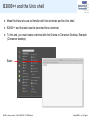
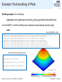
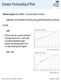
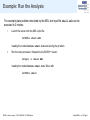
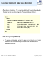
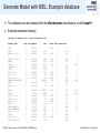
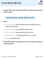
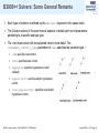
B2000++ Lecture Notes Using B2000++ Version1.2 of 13.1.2014 SMR Engineering & Development CH-2500 Bienne http://www.smr.ch B2000++ Lecture notes, © 2014 SMR SA, CH-2500 Bienne Using B2000++ (v1.2) Page 1 Content of Lecture ► Presentation of an example – Buckling of a plate ► Create a FE model with B2000++ with the Model Description language (MDL) or with the Nastran BDF converter ► Overview of MDL ► Summary of MDL model creation capabilities ► Execute B2000++ ► Summary of post-processing capabilities ► Viewing ► Scripting B2000++ Lecture notes, © 2014 SMR SA, CH-2500 Bienne Using B2000++ (v1.2) Page 2 B2000++ and the Unix shell ► Meant for those who are not familiar with Unix terminals and the Unix shell. ► B2000++ and the tools must be launched from a terminal. ► To this end, you must create a terminal with the Gnome or Cinnamon Desktop. Example (Cinnamon desktop): Select B2000++ Lecture notes, © 2014 SMR SA, CH-2500 Bienne Using B2000++ (v1.2) Page 3 Example: Post-buckling of Plate ► Example to illustrate the non-linear solid mechanics analysis capabilities of B2000++. ► Square plate made of laminated composite material. ► Loaded in-plane by a “displacement load” and out-of-plane by a concentrated load. ► Plate is simply supported. ► B2000++ shall compute: ► The linear buckling load due to in-plane “displacement loading” ► The non-linear response due to increasing in-plane “displacement loading” ► Note: The example can be found in the examples collection under <prefix>/share/doc/B2000++/examples/solid_mechanics/ static_plate_postbuckling Copy the examples to one of your directories: cp -a <prefix>/share/B2000++/test_cases/examples . B2000++ Lecture notes, © 2014 SMR SA, CH-2500 Bienne Using B2000++ (v1.2) Page 4 Example: Post-buckling of Plate Buckling analysis: Go to directory examples/solid_mechanics/static_plate_postbuckling/buckling and run B2000++ and the buckling value extraction post-processing script by typing make Output from B2000++ Solver INFO:solver.linearised_prebuckling:12:26:54.108: INFO:solver.linearised_prebuckling:12:26:54.108: INFO:solver.linearised_prebuckling:12:26:54.111: INFO:solver.linearised_prebuckling:12:26:54.395: INFO:solver.linearised_prebuckling:12:26:54.447: INFO:solver.linearised_prebuckling:12:26:54.477: INFO:solver.linearised_prebuckling:12:26:54.802: Start linearised prebuckling solver for case 1. Assemble the linear problem. Element matrix assembly Resolve the linear problem Assemble the stability matrix. Eigenvalue problem resolution End of linearised prebuckling solver Output from Python post-processing script Total force Fx [N]= 89373.4838994 Eigenvalue= 0.039875218639 Fcrit=Fx*Eigenvalue [N]= 3563.78721101 Ncrit=Fcrit/L [N/mm]= 17.8189360551 Post-processor (make view): Buckling shape and amplitude B2000++ Lecture notes, © 2014 SMR SA, CH-2500 Bienne Using B2000++ (v1.2) Page 5 Example: Post-buckling of Plate Nonlinear analysis: Run a B2000++ non-linear analysis in directory examples/solid_mechanics/static_plate_postbuckling/post_buckling by typing make ► Plot the results with a script for plotting the total edge reaction force vs. plate center out-of-plane displacement (upper diagram) and total edge reaction force vs. edge shortening (lower diagram): make view B2000++ Lecture notes, © 2014 SMR SA, CH-2500 Bienne Using B2000++ (v1.2) Page 6 Example: Run the Analysis The example plate problem described by the MDL text input file shell.mdl can be executed in 2 modes: 1. Launch the solver with the MDL input file: b2000++ shell.mdl creating the model database shell.b2m and solving the problem. 2. Run the input processor, followed by the B2000++ solver: b2ip++ -i shell.mdl creating the model database shell.b2m. Solve with b2000++ shell B2000++ Lecture notes, © 2014 SMR SA, CH-2500 Bienne Using B2000++ (v1.2) Page 7 Example: Run the Analysis ► To get information or debug information during the execution of the solver, issue one of the solver options. Note that b2000++ -h will print a short list of options and stop. ► The -l option of b2000++ allows for printing all kind of information. b2000++ -l 'info of solver in cerr' shell.mdl will print a short summary of the solver steps. Plate example: INFO:solver.linearised_prebuckling:12:26:54.108: case 1. INFO:solver.linearised_prebuckling:12:26:54.108: INFO:solver.linearised_prebuckling:12:26:54.111: INFO:solver.linearised_prebuckling:12:26:54.395: INFO:solver.linearised_prebuckling:12:26:54.447: INFO:solver.linearised_prebuckling:12:26:54.477: INFO:solver.linearised_prebuckling:12:26:54.802: B2000++ Lecture notes, © 2014 SMR SA, CH-2500 Bienne Start prebuckling solver for Assemble linear problem. Element matrix assembly. Resolve linear problem Assemble stability matrix. Eigenvalue problem resolution. End of prebuckling solver. Using B2000++ (v1.2) Page 8 Model and Analysis ► An analysis with B2000++ is performed in two steps: 1. Create the B2000++ model database, 2. Solve the problem. Both steps are executed in batch mode. ► The solver is capable of creating the database before solving the problem. The is is the usual procedure, unless one wants to view the model before starting the solver. ► A B2000++ model database can be created by ► Specifying the mesh, boundary conditions and solution parameter with the B2000++ Model Description Language (MDL), ► Converting a Nastran BDF file to an (almost) complete MDL file, ► Creating a mesh with Salome, convert it to MDL, and add boundary conditions and solution parameter with the B2000++ Model Description Language (MDL), ► User-written software, and by translating the MDL file to a B2000++ database with the B2000++ input processor b2ip++. B2000++ Lecture notes, © 2014 SMR SA, CH-2500 Bienne Using B2000++ (v1.2) Page 9 Generate Model with MDL Syntax ► A B2000++ model is generated by means of a text file containing MDL commands. The file is passed to the B2000++ input processor which translates it to database format. ► The B2000++ Model Description language is a relatively simple, easy to understand keyword-based language with some flow control capabilities. Example: set 1 title 'Forced displacement' value -1.0 dof 1 epatch 1 e2 end which means create a set no. 1 with a title and with values of -1.0 for dof (degrees-offreedom) 1 assigned to patch 1, edge e2. ► For details, see B2000++ user Manual: B2000++ User Manual > The B2000++ Model Description Language (MDL) > MDL syntax and programming B2000++ Lecture notes, © 2014 SMR SA, CH-2500 Bienne Using B2000++ (v1.2) Page 10 Generate Model with MDL Input Deck ► A B2000++ Model Description Language (MDL) input deck is composed of a series of blocks, each of them defining a specific feature of the model. ► Each block is started by the relevant keyword and terminated by end. ► Example node coordinate definitions nodes 1 0.0 0.0 0.0 2 2.5 0.0 0.0 dref 1 3 5.0 0.0 0.0 dref 0 4 0. 5. 0.0 end Nodes 1 and 2 adopt default DOF reference system, node 3 adopts DOF reference system 1, and node 4 and subsequent default system 0. B2000++ Lecture notes, © 2014 SMR SA, CH-2500 Bienne Using B2000++ (v1.2) Page 11 Generate Model with MDL Input Deck # Title title " " # Branches definitions branch id commands end # Element materials definitions emat mid id commands endmid end # Explicitly connect nodes join commands end # Linear constraints linc commands end B2000++ Lecture notes, © 2014 SMR SA, CH-2500 Bienne # Essential boundary conditions ebc commands end # Natural boundary conditions nbc commands end # Analysis cases cases commands end # Analysis directives adir commands end Using B2000++ (v1.2) Page 12 Generate Model with MDL Branch Definition ► B2000++ allows for defining branches, i.e. parts of a model with independent node, element, and boundary condition definitions. Note: If only one branch exists in the model, the branch does not have to be defined explicitly. ► Branches can then be connected with the join command. ► NASTRAN does not have the concept of branches. Thus, for NASTRAN models there is only one branch, branch no. 1. ► In case there is only one branch the branch block does not have to be defined. ► Branch block: branch id nodes ... end elements ... end ... end B2000++ Lecture notes, © 2014 SMR SA, CH-2500 Bienne branch id epatch id ... end ... end Using B2000++ (v1.2) Page 13 Generate Model with MDL: Nodes ► The nodes block: nodes id x y z ... dref id cref id ... end ► id designates the node identifier (a positive integer), the 'external node identifier'. ► x, y, z designate the coordinates with respect to the current transformation. ► dref designates the DOF transformation. Default id 0 is branch system. B2000++ Lecture notes, © 2014 SMR SA, CH-2500 Bienne Using B2000++ (v1.2) Page 14 Generate Model with MDL: Transformations ► The transformation block: transformation id type p1x p1y p1z p2x p2y p2z p3x p3y p3z ... end ► id designates the transformation identifier (a positive integer). ► type designate the type of transformation (CARTESIAN, CYLINDRICAL, SHPERICAL). ► The three points p1, p2, and p3, construct the transformation. Cartesian B2000++ Lecture notes, © 2014 SMR SA, CH-2500 Bienne Cylindrical Spherical Using B2000++ (v1.2) Page 15 Generate Model with MDL: Reference Frames ► B2000++ discerns between the following coordinate systems reference frames). ► Global system ► Branch system ► Element system ► Material system. ► Usually and per default the global system and the branch system coincide, as is the case with NASTAN meshes. B2000++ Lecture notes, © 2014 SMR SA, CH-2500 Bienne Using B2000++ (v1.2) Page 16 Generate Model with MDL: Elements ► B2000++ elements can be specified one by one, as is the case when NASTRAN BDF meshes are translated. ► Requires the nodes to be defined. ► allows for maximum flexibility with definition of material properties, shell properties, local element orientation, etc. ► B2000++ elements can be generated with the epatch command – a means for generating meshes based on simple analytical geometries. ► A patch defines nodes and elements. ► Node and element attributes are constant throughout the patch. B2000++ Lecture notes, © 2014 SMR SA, CH-2500 Bienne Using B2000++ (v1.2) Page 17 Generate Model with MDL: Elements ► The elements block: elements attributes ... eid n1 n2 ... nnne attributes ... eid [n1 n2 ... nnne] end ► Required attributes are the element type eltype t which also re-initializes all attribute definitions within the block and, for most element types, the material identifier mid id. ► Other attributes are element dependent, see element documentation. ► The element identifier eid, together with the element-to-node connectivity n1 n2 ... nnn defines elements with the attributes previously listed (or the default attributes). Brackets are required in case the number of nodes is variable. ► See the Generic Element section of the user manual for the element node, edge, and face numbering scheme. B2000++ Lecture notes, © 2014 SMR SA, CH-2500 Bienne Using B2000++ (v1.2) Page 18 Generate Model with MDL: Elements ► Example of element definition: elements eltype B2.S.MITC mid 1 section rectangular 0.3 0.01 beam_orientation 0 1 0 1 1 2 2 2 3 ... end which defines 2 node beam elements. Note that beam elements require the definition of a local frame. This is achieved with the beam_orientation defining the local beam y-axis. B2000++ Lecture notes, © 2014 SMR SA, CH-2500 Bienne Using B2000++ (v1.2) Page 19 Generate Model with MDL: Element patches ► Elements can be generated with patches, i.e. some simple pre-defined analytical geometrical forms such as 4-sided plate, cylinder, cone, cube, etc. ► Element patch block definition: epatch id geometry t geometrical_attributes ... eltype t element_attributes ... end ► One or more element patches can be generated in one and the same branch. ► However, some branches usually require translation and rotation. In this case only one patch per branch! ► More than one element patch require the join command (see later). B2000++ Lecture notes, © 2014 SMR SA, CH-2500 Bienne Using B2000++ (v1.2) Page 20 Generate Model with MDL: Element patches ► From the Introduction Example: Generate the mesh and the elements of the plate with a MDL epatch (here: with id=1). epatch 1 geometry plate p1 0. 0. 0. p2 200. 0. 0. p3 200. 200. 0. p4 0. 200. 0. ne1 20 ne2 20 # eltype Q4.S.MITC # thickness 1.6 # mid 2 # end B2000++ Lecture notes, © 2014 SMR SA, CH-2500 Bienne N. of elements in either direction Element type generated Thickness (for non laminate material) Material identifier Using B2000++ (v1.2) Page 21 Generate Model with MDL: Material ► The emat block defines all element materials which describe the physical properties of the materials assigned to the elements. emat mid id type t attributes end ... end ► Each material is identified by a positive integer id and a material type descriptor t. ► The element material is then referenced from elements etc. by the identifier id. B2000++ Lecture notes, © 2014 SMR SA, CH-2500 Bienne Using B2000++ (v1.2) Page 22 Generate Model with MDL: Material ► Example from Introduction: ► Define an orthotropic stress analysis material 1 for each layer of MITC shell elements. Define a second material of type LAMINATE. ► The shell element then gets the material reference 2 (the LAMINATE material), which in its turn references the layer material. emat mid 1 type ORTHOTROPIC e1 146.86e+03 e2 9.65e+03 e3 9.65e+03 p1 0.3 p2 0.023 p3 0.023 g1 45.5e+02 g2 45.5e+02 g3 45.5e+02 end mid 2 type LAMINATE end B2000++ Lecture notes, © 2014 SMR SA, CH-2500 Bienne lid 1 Using B2000++ (v1.2) Page 23 Generate Model with MDL: Laminates ► The laminates block allow for defining all laminates of the model, the laminates being placed in a sub-block identified by a positive identifier id. ► Each ply contains the ply number iply, the ply thickness t, the angle of orientation alpha, and the material identifier mid. laminates lid id [attributes] iply t alpha mid ... [attributes] iply t alpha mid ... end ... end Laminate orientation in element B2000++ Lecture notes, © 2014 SMR SA, CH-2500 Bienne Using B2000++ (v1.2) Page 24 Generate Model with MDL: Essential B. C. ► The ebc block defines essential boundary conditions, such as 'zero constraints' or 'displacement constraints'. ► Collections of conditions are grouped in a set identified by a positive integer. Later, in the cases blocks, these sets are referenced. ► Conditions can be generated for nodes, edges, ebc set id attributes list ... attributes list ... end ... end faces, volumes and they can be assigned to edges or faces of patches. ► Again, attributes are listed, followed by the objects such as nodes, edges, etc., to which they will be assigned. ► See B2000++ User Manual The B2000++ Model Description Language (MDL) > Global MDL Commands > ebc B2000++ Lecture notes, © 2014 SMR SA, CH-2500 Bienne Using B2000++ (v1.2) Page 25 Generate Model with MDL: Essential B. C. ► Example from Introduction: ► Create a set 1 with non-zero constraints for dof 2 of edge 2 of epatch 1. This is the edge which is going to be pushed. ► Create a set 2 with zero constraints for DOF's 3 of edges 2 and 3 of epatch 1 and DOF's 1 and 3 of edge 4. Add an additional constraint to node 1 for dof 2. This is the set which defines the plate support conditions ebc set 1 title value end set 2 title value value value value value end 'Forced displacement' -1.0 dof 1 epatch 1 e2 'Zero constraints' 0.0 dof [3] epatch 1 0.0 dof [3] epatch 1 0.0 dof [3] epatch 1 0.0 dof [1 3] epatch 0.0 dof 2 nodes 1 e1 e2 e3 1 e4 end B2000++ Lecture notes, © 2014 SMR SA, CH-2500 Bienne Using B2000++ (v1.2) Page 26 Generate Model with MDL: Natural B. C. ► The nbc block defines natural boundary conditions, such as 'forces' or 'heat sources'. ► Collections of conditions are grouped in a set identified by a positive integer. Later, in the cases blocks, these sets are referenced. ► Conditions can be generated for nodes, edges, nbc set id [parameters] attributes list ... attributes list ... end ... end faces, volumes and they can be assigned to edges or faces of patches. ► Again, attributes are listed, followed by the objects such as nodes, edges, etc., to which they will be assigned. ► See B2000++ User Manual The B2000++ Model Description Language (MDL) > Global MDL Commands > nbc B2000++ Lecture notes, © 2014 SMR SA, CH-2500 Bienne Using B2000++ (v1.2) Page 27 Generate Model with MDL: Natural B. C. ► Example from Introduction: ► For the one epatch model: Create the set 2 with a force of 2 N in the z-direction (DOF 3) of node 221. This node can be parametrized with the MDL scripting capability and the definition of variables (see input file plate1.mdl). ► For the four epatch model: Create the set 2 with a force of 2 N in the z-direction (DOF 3) of point P3 of epatch 1. Node is parametrized! # One-branch model nbc set 2 title 'Out-of-plane force' value 2. dof 3 nodes 221 end end B2000++ Lecture notes, © 2014 SMR SA, CH-2500 Bienne # Four-branch model nbc set 2 title 'Out-of-plane force' value 2. epatch 1 p3 end end Using B2000++ (v1.2) Page 28 Generate Model with MDL: Case definition ► The cases block defines all ingredients needed for one or more specific states referred to as cases. One or more cases can be defined in the case sub-blocks. Each case is identified by the case identifier id. Specifically, a case ► Adds boundary conditions sets to a case cases case id attributes end case id attributes end ... end ► Defines set names (optional) ► Defines solution type and strategy ► Many of the attributes in a case are solution type dependent. The relevant sections of the user manual explain all parameters pertaining to a specific solution type. B2000++ Lecture notes, © 2014 SMR SA, CH-2500 Bienne Using B2000++ (v1.2) Page 29 Generate Model with MDL: Case definition ► Examples from Introduction: The first analysis calculates the linear buckling load under the given boundary condition configuration. The associated case definition is cases case 1 analysis linearised_prebuckling # Analysis type nmodes 10 # Compute 10 eigenmodes around 0.0 ebc 1 # Include displacement constraint set 1 (ebc) ebc 2 # Include zero-value constraint set 2 (ebc) nbc 2 # Include Force set 1 (nbc) endcase end ► Note the analysis keyword hierarchy: ► The analysis method analysis specified in the adir command defines the overall analysis method for all cases, except when analysis is specified in the case block, where is supersedes the overall one. B2000++ Lecture notes, © 2014 SMR SA, CH-2500 Bienne Using B2000++ (v1.2) Page 30 Generate Model with MDL: Case definition ► Examples from Introduction: The second analysis calculates the nonlinear response under the given boundary condition configuration. The associated case definition is cases case 1 analysis nonlinear increment_control_type load # Load control (no continuation) ebc 1 # Include displacement constraint set 1 (ebc) ebc 2 # Include zero-value constraint set 2 (ebc) nbc 2 # Include Force set 1 (nbc) step_size_init 0.01 # Initial step size step_size_max 0.1 # Maximum step size # to get some points on the curve! step_size_min 0.001 # Minimum step size (IMPORTANT!) endcase end B2000++ Lecture notes, © 2014 SMR SA, CH-2500 Bienne Using B2000++ (v1.2) Page 31 Generate Model with MDL: Analysis Directives ► The adir tells the solver which cases to process during the run. list contains one or more case identifiers. If more than one identifier is specified, the identifiers must be placed between square brackets [...]. adir cases list Other attributes… end ► Example from the Introduction: adir cases 1 end adir cases [1] end adir cases [1 2] end ► See B2000++ User Manual The B2000++ Model Description Language (MDL) > Global MDL Commands > cases B2000++ Lecture notes, © 2014 SMR SA, CH-2500 Bienne Using B2000++ (v1.2) Page 32 Generate Model with MDL Other Commands ► title Specifies an optional problem title. ► join connects branches and/or patches. ► linc defines linear constraints. ► dof_init and dofd_init define initial conditions for transient analysis. B2000++ Lecture notes, © 2014 SMR SA, CH-2500 Bienne Using B2000++ (v1.2) Page 33 Generate Model with MDL: Example database ► The database can be browsed with the b2mcbrowser data browser or with baspl++ ► Example database directory: Contents of database file "./shell.b2m/archives.mc": dataset_name ADIR BDTB.1 BMODE.1.0.0.1.1 ... BMODE.1.0.0.1.10 BNFP.1 CASE.1 CONSTANTS COOR.1 DISP.1.0.0.1 EBC.1.0.0.1 EBC.1.0.0.2 ELEMENT-PARAMETERS ELMA.1 EMAT.0.0.0.1 … ETAB.1 FIELDS FORC.1.0.0.1 LAMI.0.0.0.1 NBC.1.0.0.2 NODA.1 NODE-NORMALS.1 NODE-PARAMETERS NODS.1.0.270.0 PATCH.1 RCFO.1.0.0.1 SOLUTION.0.0.0.1 type file_address size dsize ndim dimensions I $ F 4615240 4263072 4918728 1 8192 2205 8192 0 4096 1 1 2 1 8192 441, F I $ $ F F F F $ I F 5266416 4525856 4598848 4197504 4538776 4841464 4561216 4565816 0 4556416 4581320 2205 2205 12288 4096 1323 2205 63 318 4096000 1200 68 4096 4096 4096 0 0 4096 4096 4096 8192 0 4096 2 2 2 1 2 2 2 2 2 2 1 441, 441, 3, 4096 441, 441, 21, 106, 1000, 400, 68 $ $ F F F I F $ I $ F $ 4275360 4201600 4802832 4576576 4572456 4549360 4775352 4104192 4519456 4271264 4880096 5288152 240000 61440 2205 80 3 1764 1323 9216 1600 4096 2205 4096 4096 0 4096 4096 4096 0 0 0 0 0 4096 0 2 2 2 2 2 2 2 2 2 1 2 1 400, 30, 441, 16, 1, 441, 441, 18, 400, 4096 441, 4096 B2000++ Lecture notes, © 2014 SMR SA, CH-2500 Bienne 5 5 5 4096 3 5 3 3 4096 3 600 2048 5 5 3 4 3 512 4 5 Using B2000++ (v1.2) Page 34 Convert Nastran BDF deck ► The Nastran BDF converter reads a Nastran BDF file and translates (most) of the deck to a B2000++ MDL file. b2convert_from_nas [options] bdf-file mdl-file ► Options: ► -coor-scale=factor scales all coordinates, thicknesses, and offsets by a factor. Also scaled are non-structural masses. ► -dof-scale=factor scales all specified DOF's (ebc's) by a factor. ► -force-scale=factor scales all specified forces (nbc's) by a factor. ► -permute=[X|x|Y|y|Z|z] specifies permutation for the x-, y-, and z-axes. ► -verbose produces verbose output. ► Note that BDF instructions not understood by the converter are listed in the beginning of the generated MDL file. B2000++ Lecture notes, © 2014 SMR SA, CH-2500 Bienne Using B2000++ (v1.2) Page 35 B2000++ Solvers: Some General Remarks Each type of solution is defined by the analysis keyword in the cases block. The Solvers section of the user manual explains in detail each set of parameters pertaining to a specific analysis type. The non-linear solver will be explained here in more detail. The increment_control_type parameter of case specifies the predictor type t: load specifies load control state specifies state control hyperplane specifies hyperplane control (default) hyperelliptic specifies elliptic hyperplane control local_hyperelliptic specifies local elliptic hyperplane control B2000++ Lecture notes, © 2014 SMR SA, CH-2500 Bienne Using B2000++ (v1.2) Page 36 Post-Processing: The baspl++ Viewer baspl++ is a viewing and post-processing tool fully integrated in B2000++: It allows for viewing most of the mesh and solution of a B2000++ model. It also allows for on-line viewing (during solution process). The Python based scripting language allows for extracting and displaying of text-based output. In addition, baspl++ also understands other solvers and formats for multi-disciplinary analysis (not discussed here). This short introduction describes Some elementary viewing functions Some elementary scripting functions B2000++ Lecture notes, © 2014 SMR SA, CH-2500 Bienne Using B2000++ (v1.2) Page 37 The baspl++ Viewer: Launch ► baspl++ is launched from the terminal (shell) with baspl++ [options] [database(s)] [script [argument(s)] or from a Python script (see later) or with the GUI. ► Example: Launch baspl++ for viewing the plate problem of the introduction baspl++ -t shell.b2m which launches the viewer with the baspl++ interpreter (Python console) in the launching shell and baspl++ shell.b2m which launches the viewer with the interpreter (Python console) in the GUI (see next slide). B2000++ Lecture notes, © 2014 SMR SA, CH-2500 Bienne Using B2000++ (v1.2) Page 38 The baspl++ Viewer: Objects baspl++ top-level window (object): The Models The Renderers The Scenes B2000++ Lecture notes, © 2014 SMR SA, CH-2500 Bienne Using B2000++ (v1.2) Page 39 The baspl++ Viewer: Objects ► baspl++ main objects (classes): ► Some objects for viewing meshes and solutions: ► Model (Models): Contains a B2000++ model database with mesh. ► Field: Contains a solution field. ► NPart (Renderers): Extracts or cuts – for rendering - elements, nodes, interpolates solution fields. ► Tracer: Computes 3D particle traces from Model object and velocity solution field(s) and renders them. ► Objects for XY (graph) plotting ► Curve: A container for x/y-values. ► Graph: Contains a set of Curve objects and renders them. ► Applets and tools. ► Plus others (see baspl++ user manual). B2000++ Lecture notes, © 2014 SMR SA, CH-2500 Bienne Using B2000++ (v1.2) Page 40 The baspl++ Viewer: View mesh ► To view a mesh and solutions Open a B2000++ model database or pass the database name with the command line. With the right mouse button, select Create empty NPart from the Model shell.b2m: 1. Click with right mouse button 2. A new renderer NPart_1 is created 3. The renderer context is displayed B2000++ Lecture notes, © 2014 SMR SA, CH-2500 Bienne Using B2000++ (v1.2) Page 41 The baspl++ Viewer: View mesh ► Extract all elements: Displays mesh without edges Check extract button B2000++ Lecture notes, © 2014 SMR SA, CH-2500 Bienne Using B2000++ (v1.2) Page 42 Post-Processing The baspl++ Viewer: View mesh Select Display menu and check Edge box: View edges 1. Check edge box 2. Displays mesh with edges B2000++ Lecture notes, © 2014 SMR SA, CH-2500 Bienne Using B2000++ (v1.2) Page 43 The baspl++ Viewer: View solution To add i.e. amplitude of buckling mode, start by extracting the mode in the Field menu: 4. Return to previous 2. Select field and mode no. (double click!) 1. Add a field extraction 3. Apply B2000++ Lecture notes, © 2014 SMR SA, CH-2500 Bienne Using B2000++ (v1.2) Page 44 The baspl++ Viewer: View solution To view amplitude of buckling mode, select extracted field (BMODE.1.1) and check amplitude in Component menu: Select field B2000++ Lecture notes, © 2014 SMR SA, CH-2500 Bienne Using B2000++ (v1.2) Page 45 The baspl++ Viewer: Save Script To save the script which generates the current view, select Create script from File menu and type a file name: Restart with file name and restore view: baspl++ myview.py B2000++ Lecture notes, © 2014 SMR SA, CH-2500 Bienne Using B2000++ (v1.2) Page 46 The baspl++ Viewer: Scripting Python-scripting example: Extract the buckling analysis eigenvalue and transform to critical load (see file buckling_load.py in the buckling examples directory). The script ► Creates a baspl++ Modes objects, which computes, for the particular case of a displacement loading the total reaction force Fx due to the forced displacement. the total critical load Fcrit Fcrit=Fx * Eigenvalue ► Computes the critical load per unit length of the plate Ncrit Ncrit =Fcrit / L where L is the plate edge length. Python code: o = Modes() # Ceate Modes object o.part = p # Add current part to Model objects Fcrit = o.details[0].critical_force # Get critial force s.label = "Fcrit=Fx*Eigenvalue [N]=%g, \ Ncrit=Fcrit/L [N/mm]=%g" % (Fcrit, Fcrit/200.) B2000++ Lecture notes, © 2014 SMR SA, CH-2500 Bienne Using B2000++ (v1.2) Page 47