Download MDStressLab User Manual version 1.0.0

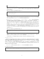
MDStressLab User Manual Version 1.2.0
Nikhil Chandra Admal, Min Shi and E. B. Tadmor
Department of Aerospace Engineering and Mechanics
University of Minnesota, Minneapolis, MN 55455, USA
1. Introduction
This is the user manual for MDStressLab, a computer program for post processing molecular statics (MS) and
molecular dynamics (MD) results to obtain stress fields using different definitions of the atomistic stress tensor. The
latest version of the code and this user manual are available online at http://mdstresslab.org. When making
use of this code, please cite the following articles by Admal and Tadmor upon which it is based:
1. Admal, N. C., Tadmor, E. B., 2010. A unified interpretation of stress in molecular systems. Journal of Elasticity
100, 63–143
2. Admal, N. C., Tadmor, E. B., 2011. Stress and heat flux for arbitrary multibody potentials: A unified framework.
The Journal of Chemical Physics 134, 184106
3. Admal, N. C., Tadmor, E. B., 2016b. The non-uniqueness of the atomistic stress tensor and its relationship to
the generalized Beltrami representation. Journal of the Mechanics and Physics of Solids 93, 72–92
4. Admal, N. C., Tadmor, E. B., 2016a. Material fields in atomistics as pull-backs of spatial distributions. Journal
of the Mechanics and Physics of Solids 89, 59–76
1.1. Stress Definitions
The most commonly used atomistic stress definitions are the Hardy (1982), Virial (Maxwell, 1870, 1874) and Tsai
(1979) stress tensors. For a given choice of weighting function w, the Hardy stress σw at a point x ∈ R3 and time t is
given by
σw (x, t) = σw,v (x, t) + σw,k (x, t),
Z
1X 1
[−fαβ w((1 − s)xα + sxβ − x) ⊗ (xα − xβ )] ds,
σw,v (x, t) =
2
s=0
(1)
(2)
α,β
α6=β
σw,k (x, t) = −
X
α
mα (vαrel ⊗ vαrel )w(xα − x),
(3)
where xα ∈ R3 and vα ∈ R3 denote the position and velocity of particle α in the deformed configuration, fαβ is
the force between particles α and β, and vαrel is the relative velocity of particle α with respect to the particles in its
neighborhood.1 The summations in (2) and (3) are over all particles, and the summation in (2) is a double summation.
The Tsai and virial stress tensors are obtained from the Hardy stress as special cases (Admal and Tadmor, 2010). The
Tsai stress tensor is obtained from (1) as a limit of σw for a sequence of weighting functions whose support collapses
to a plane l. For a plane l with normal n and area A, the Tsai traction vector is given by
t(x, n) =


Z
T
X
1  T X
(xα − xβ ) · n
mα vα (t↔ )(vα (t↔ ) · n) 
lim
fαβ
dt −
,
T →∞ AT
|(xα − xβ ) · n|
|vα (t↔ ) · n|
0
αβ∩l
1 See
(4)
α↔l
rel .
Admal and Tadmor (2016b) and Admal and Tadmor (2016a) for the definition of vα
Preprint submitted to Journal of Mechanics and Physics of Solids
August 2, 2017
where the first summation is over all bonds that cross the plane, the second summation is over all particles that cross
the plane, and vα (t↔ ) denotes the velocity of particle α at the time it crosses the plane l. The virial stress is obtained
from the Hardy stress by taking a constant weighting function, and neglecting bonds that cross or exit the averaging
domain in the summation given in (1).
The atomistic stress tensors described above are defined on the deformed configuration of particles and correspond
to the spatial Cauchy stress (or true stress) defined in continuum mechanics. To make this clear, in the following the
prefix “Cauchy” is used when referring to spatial stress measures.
At the same time, in continuum mechanics the stress tensor also has a material description in terms of the first
Piola–Kirchhoff stress. In the absence of an explicit deformation mapping, it is uncommon to give a material description of the atomistic stress tensor. However, in Admal and Tadmor (2016a), we have shown that there exists a material
description of the atomistic stress in the form of an atomistic Piola–Kirchhoff stress. In particular, for a given reference
and deformed configuration of particles, Xα and xα respectively, we have shown that the Hardy version of the first
Piola–Kirchhoff stress is given by
P (X, t) =
XZ
α,β
α<β
1
s=0
[−fαβ w((1 − s)Xα + sXβ − X) ⊗ (Xα − Xβ )] ds,
(5)
where fαβ is evaluated for a deformed configuration of particles. Some notable features of the first Piola–Kirchhoff
atomistic stress is its non-symmetry and the absence of a kinetic contribution. Similar to the derivation of the Cauchy–
Tsai and the Cauchy–virial stress tensors, their Piola counterparts can be obtained as special cases of (5).
1.2. Non-uniqueness of the atomistic stress tensor
The non-uniqueness of the potential part of the atomistic stress tensor due to the non-uniqueness of force decomposition, i.e. the non-uniqueness of the forces fαβ , is a well-known issue. Admal and Tadmor (2010) show that this
non-uniqueness is directly related to the non-uniqueness of the potential energy representation as a function of distances. In Admal and Tadmor (2016b) we propose a decomposition of the atomistic stress into a unique irrotational
part (independent of the potential energy representation) and a non-unique solenoidal (divergence-free) part which
depends on the choice of the potential energy representation. Additionally, it is shown that this decomposition has
an interesting analog in continuum mechanics in the form of a generalized Beltrami representation, which itself is an
analog for symmetric tensor fields of the Helmholtz decomposition of vector fields.
1.3. MDStressLab stress calculations and required input
The MDStressLab code can calculate fields of the Cauchy and first Piola–Kirchhoff versions of the Hardy, Tsai
and virial stress tensor for three-dimensional systems. The user defines a grid of points and the stress is evaluated at
all grid points. Additionally, the decomposition studied in Admal and Tadmor (2016b) can be carried out on each of
these stress tensors.
Examining the definitions given in equations (1)–(5), we see that the stress tensor code requires the following
input:
• Reference and deformed configuration of particles.
• Velocities of particles.
• The species of each particle (used to identify its mass and used by the force calculations with the interatomic
model).
• Details of the periodic boundary conditions (PBCs) and the initial and final size of the box used to prescribe the
PBCs. In the present version, we restrict ourselves to orthogonal periodic boundary conditions.
• The potential representation used to evaluate the forces fαβ . This is an interatomic model compatible with
the application programming interface (API) of the Knowledgebase of Interatomic Models (KIM) as described
below.
• The weighting function used to evaluate the Hardy stress tensor. In the present version of the code, the compact
support of the weighting function is taken to be a sphere of radius ravg specified by the user. The Tsai stress
tensor at a point x is constructed using the Tsai traction vector evaluated at x on three equal squares parallel to
the three axes. The length of the squares is taken to be 2ravg .
2
1.4. Units
The units used by the MDStressLab program are:
• Distance: Å
• Energy: eV
• Time: ps
• Mass: eV · ps2 /Å
2
In the next section, the format of the input file to MDStressLab is described.
2. Input file
Below is a sample input file to MDStressLab. This is followed by a detailed explanation of the commands that
appear in it.
% Read in atomic configuration and species information
read
spec,species
conf,config
end
% Set up the grid for computing the stress field
grid
gfit,300,300,0
end
% Define the KIM model used to compute the atomic interactions
potential
modl,Pair_LJ_Smooth_Bernardes_Ar__MO_764178710049_000
end
% Specify whether to decompose stress into unique and non-unique parts
uniqueness
project,T
end
% Setup and begin stress calculation
stress
cauchy,T
pkstr,F
hardy,T
virial,F
tsai,F
avgsize,8.0
weight,constant
end
stop
The input file consists of six stages: read, grid, potential, uniqueness, stress and stop. Any text
following a % symbol is treated as a comment. Each stage (except stop) contains commands and their associated
arguments in the following format:
3
command,value_1,value_2,...
Each stage (except stop) ends with an ’end’ command. The six stages are described separately below. Note that
the six stages must be included in the input file in the order shown in the example below, otherwise incorrect behavior
may result.
2.1. Stage ’read’
In this stage, the state of the system is read as an input from a configuration file and a species file. The two files are
expected to have an extension .data. The configuration and species files are specified using the commands conf and
spec, respectively. For example, in the input file shown above, the conf commands reads in the configuration file
’config.data’, and the spec commands reads in the species file ’species.data’. If no file names are specified, the files ’config.data’ and ’species.data’ will be read in by default. The format for the configuration
file is shown below.
3
<n=Number of atoms>
<Initial box size>
<Final box size>
<Periodic boundary conditions>
<Species_1>
<Position_1>_i
<Velocity_1>_i
<Species_2>
<Position_2>_i
<Velocity_2>_i
.. .. .. .. .. .. .. .. .. .. .. .. .. ..
<Species_n>
<Position_n>_i
<Velocity_n>_i
<Species_1>
<Position_1>_f
<Velocity_1>_f
<Species_2>
<Position_2>_f
<Velocity_2>_f
.. .. .. .. .. .. .. .. .. .. .. .. .. ..
<Species_n>
<Position_n>_f
<Velocity_n>_f
The subscripts i and f shown above correspond to initial and final configurations. The <PBC> field accepts a 3dimensional logical (boolean) array indicating whether or not (T/F) each of the Cartesian directions is periodic. The
fields <Box size_i> and <Box size_f> accept a 3-dimensional double precision array. The value of the final
box size (in all periodic directions) must be greater than twice the cutoff of the interatomic model. The <Species_k>
field is a string of length 2 or 3 of the element name. A snippet of a configuration file of Argon atoms is shown below.
3
58260
1000.00
1000.00
26.46
F
F
T
Ar
-129.658 -148.180
Ar
-129.658 -148.180
Ar
-129.658 -148.180
..
1000.00
2.6460
13.230
7.9382
1000.00
0.00
0.00
0.00
0.00
0.00
0.00
26.46
0.00
0.00
0.00
Note that the order of the atomic positions in the final configuration should be identical to the order of the atomic
positions in the initial configuration. The species file contains masses of different species of atoms. The format of the
species file is shown below.
<Species_1>
<mass_1>
<Species_2>
<mass_2>
..
<mass_nsp_file> <mass_nsp_file>
A sample species file is given below.
Al
Ar
Si
0.0026981
0.0039948
0.0028085
4
2.2. Stage ’grid’
In this stage, the grid on which the atomistic stress will be evaluated is constructed. There are three different
options for specifying the grid points: gfit, gfile and gdef. Each grid point is a 3-dimensional array. For PBC
conditions, all grid points must lie inside the periodic box, and the distance between any grid point and the box sides2
must be greater than or equal to the size of the averaging domain.3 The grid commands and their arguments are
described below.
• gfit,<div_1,...,div_3> (double precision): This command defines a uniform grid fit to the box. The
number of divisions in the x, y and z directions for the grid are given by the arguments <div_1>, <div_2>
and <div_3>, respectively. The total number of grid points generated by gfit is equal to (<div_1>+1)
×(<div_2>+1)×(<div_3>+1). If one of the divisions is set to zero the grid becomes two dimensional
and is located at the origin of the corresponding axis. For example for <div_3>=0, the 2D grid is positioned
at z = 0. The grid is constructed such that all grid points lie inside the smallest rectangular box enclosing the
sample, and at a distance greater than ravg (averaging domain size) from the sides of the box.
As an example, below is the grid stage from the sample input file given at the start of Section 2:
grid
gfit,300,300,0
end
The above command generates a two-dimensional grid perpendicular to the z-axis. The number of divisions in
the x and y direction is 300.
The grid for Cauchy stress is built in the deformed configuration, and the grid for first Piola-Kirchhoff stress is
built in the reference configuration. By default, both grids are constructed and stored in the files grid_cauchy.data
and grid_pk1.data for later use. Different grid filenames can be specified by adding arguments to the command line a shown below. Note the double commas in the command.
grid
gfit,300,300,0,,<grid filename for Cauchy>,<grid filename for pk1>
end
The grids for either the Cauchy stress or first Piola-Kirchhoff stress or both can be explicitly requested by the
following commands:
grid
gfit,300,300,0,cauchy,<grid filename for Cauchy>
gfit,300,300,0,pk1,<grid filename for pk1>
end
• gfile,<grid filename for Cauchy>,<grid filename for pk1>: This command reads the
grid definitions from the files <grid filename for Cauchy>.data and <grid filename for
pk1>.data. One of the filenames can be omitted if no grid information is to be read for it. The format
for the grid file is shown below.
<Grid point position_1>
<Grid point position_2>
2 Three sides of the box are defined by the minimum of the x, y and z coordinates of all particles, and three parallel sides are obtained by
offsetting the minimum sides in the x, y and z directions by Lx , Ly and Lz , respectively.
3 We place this restriction due to the following reason. In order to calculate the atomistic stress at a grid point, the program loops over all
bonds that cross the averaging domain centered at the grid point. Under periodic boundary conditions, for a grid point close to the boundary of the
bounding box, there are three different kinds of bonds that cross the averaging domain: bonds which lie entirely in the box, bonds that cross the
boundaries of the box, and bonds that lie entirely in an image of the box. The program does not loop over bonds that lie entirely in the image of the
box. All grid points that lie at distance greater than ravg from the box sides, do not contain such bonds in their averaging domains.
5
.. .. .. .. .. .. .. ..
<Grid point position_ng>
Here <Grid point position_i> are the coordinates of the i-th grid point (three space delimited double
precision numbers).
Below is an example of a grid definition using gfile.
grid
gfile,grid_cauchy
gfile,,grid_pk1
end
The above command reads the positions of the grid points from a file named grid_cauchy.data for cauchy
stress and a file named grid_pk1.data for the first Piola-Kirchhoff stress.
• gdef,<val_1,...,val_3>,<len_1,...,len_3>,<div_1,...,div_3>: This command defines
a grid whose center is given by the argument <val_1,...,val_3>. The lengths of the grid in the x, y
and z directions relative to the box size in each direction are given by <len_1>, <len_2> and <len_3>,
respectively. Their values lie in the interval [0, 1]. Finally, the number of divisions in the x, y and z directions are
given by <div_1>, <div_2> and <div_3>, respectively. The total number of grid points generated by gdef
is equal to (<div_1>+1)×(<div_2>+1)×(<div_3>+1). If one of the divisions is set to zero the grid
becomes two dimensional and is located at the origin of the corresponding axis. For example for <div_3>=0,
the 2D grid is positioned at z = 0. The generated grids are stored in the files grid_cauchy.data and
grid_pk1.data for later use. The names of the grid filenames can be changed and grids can be selected as
explained for gfit.
Below is an example of a grid definition using gdef.
grid
gdef,0.0,0.0,0.0,1.0,0.5,1.0,300,300,0
end
The above command generates a two-dimensional grid beginning at the origin with lengths in the x, y directions
equal to <box size_1> and 0.5×<box size_2>, respectively.
Note that in the case of multiple definitions of the grid, only the last command will be executed.
2.3. Stage ’potential’
In this stage, the interatomic model (potential or force field) used to obtain the interatomic forces is specified.
MDStressLab is a KIM-compliant program, which means that it works with interatomic models that are compatible
with the KIM Application Programming Interface (API) (see https://openkim.org). In order to use KIM
models, it is necessary to install the KIM API framework. This is a prerequisite for using MDStressLab. See the
INSTALL_KIM file for instructions on how to install the KIM API and accompanying model files. The name of the
KIM model is given using the command
• modl,<val> (Character(len=128)), where <val> is the extended KIM ID of the model.
For example, the command
potential
modl,Pair_LJ_Smooth_Bernardes_Ar__MO_764178710049_000
end
6
(taken from the input file given at the start of Section 2) couples MDStressLab to a model with the extended KIM
ID “Pair_LJ_Smooth_Bernardes_Ar__MO_764178710049_000”. This model (Admal, 2015) describes Ar using a
modified Lennard–Jones potential.
In order to compute the various notions of the atomistic stress tensor, MDStressLab couples to a KIM compliant
model and outsources the computation of interatomic forces to the model. During this process, MDStressLab and
the coupled model constantly exchange information. The KIM API ensures that a consistent exchange of information
happens by performing an appropriate hand-shaking procedure at the beginning of the computation. This hand-shaking
is performed by comparing the KIM descriptor files4 of MDStressLab and the KIM model. The current version of
MDStressLab couples with KIM models with the following capabilities:
1. Since the units of MDStressLab are fixed, it can only work with models that support these units or models whose
units are flexible.
2. The computation within a model requires a neighbor list corresponding to a given configuration of particles.
Within the framework of KIM API, a neighbor list and its accessibility come in various forms. For example,
a neighbor list can be “half-neighbor” list or a “full-neighbor” list, both of which can be accessible through a
“locator mode”, “iterator mode”, or a combination of these two modes. The current version of MDStressLab
offers half- and full-neighbor lists accessible through iterator and locator modes.
3. Currently MDStressLab supports systems with the following neighbor boundary conditions (NBC): MI_OPBC_H,
NEIGH_PURE_H, MI_OPBC_F and NEIGH_PURE_F.
4. Since the atomistic stress tensor field depends on the derivative of the energy with respect to distances between
particles, MDStressLab can only couple to models that can compute this derivative. Within the framework of
the KIM API, this capability is described by “process_dEdr”. Thus only models that support process_dEdr can
couple to MDStressLab.
2.4. Stage ’uniqueness’
In this stage, we specify options related to the decomposition of the atomistic stress into an irrotational part and a
solenoidal part. This stage consists of only one command:
• project,<val> (logical): If <val>=T (true), the decomposition of the atomistic stress into an irrotational
part and a solenoidal part is performed. Details of the decomposition are given in Admal and Tadmor (2016b).
2.5. Stage ’stress’
In this stage, input data and options required to compute various notions of the atomistic stress tensor are specified,
including the size of the averaging domain. The following commands may be used:
• cauchy,<val> (logical): If <val>=T (true), the Cauchy stress is evaluated on the deformed configuration.
Default <val>=T.
• pkstr,<val> (logical): If <val>=T (true), the first Piola–Kirchhoff stress is evaluated on the reference
configuration. Default <val>=T.
• hardy,<val> (logical): If <val>=T (true), the Hardy stress is evaluated. Default <val>=F (false), specified
for both the Cauchy and first Piola-Kirchoof stress.
hardy,T,cauchy
hardy,false,pk1
Note that in the <val> field, only the first character is evaluated. A value of T or t is taken to be true. A value
of F or f is taken to be false.
4 A KIM descriptor file is a standard formatted file associated with a KIM model or KIM-compliant code that describes its capabilities and the
information that it can receive and provide.
7
• virial,<val> (logical): If <val>=T (true), the virial stress is evaluated. Default <val> = F (false). The
same additional information can be provided as for hardy.
• tsai,<val> (logical): If <val>=T (true), the Tsai stress is evaluated. Default <val> = F (false). The
same additional information can be provided as for hardy.
• avgsize,<val> (double precision): The value of ravg described in Section 1. Default <val>=1.0_dp.
The same additional information can be provided as for hardy.
• weight,<val> (character): The weighting function described in Section 1 used to compute the Hardy stress.
The valid options are either <val>=constant or <val>=mollify. Default <val>=constant. The
same additional information can be procided as for hardy.
MDStressLab currently supports a constant weighting function, with or without a mollifying function to smooth
the end, in a Hardy stress evaluation. The mollified weighting function is (Admal and Tadmor, 2011)

 c if r < R − δ
1
R−r
(6)
w(r) =
c 1 − cos δ π
if R − δ < r < R ,
 2
0
otherwise
In this expression, R is the radius of the sphere which forms the compact support, δ = 0.12R, and c is chosen
such that the weighting function satisfies the normalization condition:
Z
w(r)dr = 1.
(7)
R3
As an example, below is the stress stage from the sample input file given at the start of Section 2:
stress
cauchy,T
pkstr,F
hardy,T
virial,F
tsai,F
avgsize,8.0
weight,constant
end
The above command is used to compute the Cauchy version of the Hardy stress tensor using a spherical averaging
domain of radius 8 Å with a constant weighting function.
2.6. Stage ’stop’
This stage terminates the program in an orderly fashion, freeing any allocated storage and exiting gracefully.
3. Output files
The output from MDStressLab is directed to standard output and contains information about the progress of the
simulation. In addition, the various stress tensor fields requested in the input file are output to external files as described
below.
• The potential part of the Hardy, virial and Tsai stress tensors are outputted to the files hardy.str, virial.str
and tsai.str, respectively.
• The kinetic component of an atomistic stress is outputted to a file with a suffix _kin.str. For instance, the
kinetic component of the Hardy stress is outputted to the file hardy_kin.str.
8
• The decomposition of the potential part of the atomistic stress tensor is given by evaluating the irrotational and
the solenoidal parts, and outputting them to files with a suffixes _i.str and _s.str respectively, e.g. the irrotational and solenoidal parts of the Hardy stress can be found in the files hardy_i.str and hardy_s.str
respectively.
For example, the solenoidal part of the first Piola–Kirchhoff–Hardy stress tensor will be output to a file named
hardy_s_pk1.str.
All str output files consist of 12 columns and a number of rows equal to the number of grid points for either
evaulating the cauchy or 1st pk stress. The first three columns are the coordinates of the grid points, and the next nine
columns are the components of the stress tensor in the following order: 11, 21, 31, 12, 22, 32, 13, 23, 33.
4. Examples
The following two examples are included with the MDStressLab code.
4.1. Uniaxial strain
An example of a silicon under uniaxial strain is provided with the MDStressLab code. In this example, various
stress measures are computed for a strained single crystal cube of silicon in the diamond cubic crystal structure such
that the x, y and z axis are oriented along the [100], [010], and [001] crystallographic directions. The system is
deformed with a strain of 1% in the y direction, and zero strain in the x and z directions. In addition, the decomposition
of stress into an irrotational part and a solenoidal part is performed. The system is studied under zero temperature.
The intial and final configurations are obtained using LAMMPS (Plimpton, 1995) in the form of two .dump files.
The LAMMPS input script in.uniaxialstrain to generate the .dump files is included with this example. Using LAMMPS, the reference configuration of the cube is obtained by stacking 10 × 10 × 10 unit cells with a lattice
parameter a0 = 5.430950Å under flexible periodic boundary conditions. The interatomic potential is a three-body
Stillinger–Weber potential archived in OpenKIM (Singh (2016); Wen (2016); Elliott and Tadmor (2011)). The reference and deformed configurations are generated in the files dump.initial.0 and dump.final.1, respectively. These files
are converted to the MDStressLab configuration file format (see Section 2.1) using the executable script dump2str
included in the utils/ directory. This example is contained in the directory examples/Uniaxial_strain,
which contains the following files:
• README: Contains instructions for how to run the example.
• in.uniaxialstrain: The LAMMPS input script file used to generate the reference and deformed configuration dump files.
• dump.initial.0: A LAMMPS generated .dump configuration file that contains the positions of atoms
corresponding to the reference configuration.
• dump.final.1: A LAMMPS generated .dump configuration file that contains the positions of atoms corresponding to the deformed configuration.
• species.data: Contains the mass of the atomic species involved. See Section 2.1 for more information.
• testrun.in: The input file to MDStressLab setting up the problem and defining what needs to be computed.
Note that since the .dump files are included in the directory, the user does not need to have LAMMPS installed
to generate them.
Warning: the cfg files use scaled coordinates which will generate huge numerical errors during MDStressLab
calculation. We strongly recommand using unscaled/exact coordinates to perform the computation.
9
y
R
−tx
x
tx
H
H
Figure 1: A schematic of the geometry of the studied boundary-value problem, with non-zero traction boundary conditions enforced on a part of
the boundary as shown.
4.2. Plate with a hole
An example of a rectangular anisotropic medium with a hole subjected to a uniaxial loading under plane strain
conditions is provided with the MDStressLab code. As part of the example various stress measures are computed and
the decomposition into the unique (irrotational) and non-unique (solenoidal) parts is performed. A schematic of the
body showing the relevant dimensions and the boundary conditions is shown in Fig. 1. The size of the body, radius of
the hole and applied traction shown in Fig. 1 are
H = 198 Å,
R = 50 Å,
and
3
t̄x = 7.117 × 10−5 eV/Å .
(8)
The body extends to infinity in the positive and negative z-directions (i.e. periodic boundary conditions are applied
in the out-of-plane direction). The material model is taken to be a single crystal Ar in the face-centered cubic (fcc)
structure such that the x, y and z axes are oriented along the [100], [010] and [001] crystallographic directions. The
system is studied at zero temperature.
The boundary-value problem discussed above is input to the MDStressLab code in the form of reference configuration, final configuration and the potential energy model for the interaction of Ar atoms. The reference (unloaded) configuration of the plate is obtained by stacking 37×37×4 unit cells with lattice parameter a0 corresponding to the stress
free state of the chosen potential model, and removing all atoms that fall inside a circle of radius 50 Å positioned at the
center of the stack, with its out-of-plane axis parallel to the [001] crystallographic axis. The resulting system consists
of 18032 atoms. The interatomic potential is a modified Lennard–Jones pair potential archived in OpenKIM (Admal,
2015; Tadmor et al., 2011). The final configuration is obtained by displacing the atoms in the reference configuration
according to the numerical solution of the traction boundary-value problem described above. For a full discussion of
the problem, see Admal and Tadmor (2016b). This example is contained in directory examples/Plate_w_hole.
5. Utilities
A C++ script to convert LAMMPS dump (.dump) files to the configuration file format (see Section 2.1) of MDStressLab is included in the utils/ directory. The format of the .dump files for this script to work is described in the
utils/README file. Note that you need to compile the C++ script to make it work for you. An option to use g++ to
compile is:
g++ dump2str.cpp -o dump2str
10
References
Admal, N. C., 2015. Modified Lennard–Jones potential for Argon.
URL https://openkim.org/cite/MO_764178710049_000
Admal, N. C., Tadmor, E. B., 2010. A unified interpretation of stress in molecular systems. Journal of Elasticity 100,
63–143.
Admal, N. C., Tadmor, E. B., 2011. Stress and heat flux for arbitrary multibody potentials: A unified framework. The
Journal of Chemical Physics 134, 184106.
Admal, N. C., Tadmor, E. B., 2016a. Material fields in atomistics as pull-backs of spatial distributions. Journal of the
Mechanics and Physics of Solids 89, 59–76.
Admal, N. C., Tadmor, E. B., 2016b. The non-uniqueness of the atomistic stress tensor and its relationship to the
generalized Beltrami representation. Journal of the Mechanics and Physics of Solids 93, 72–92.
Elliott, R. S., Tadmor, E. B., 2011. Knowledgebase of interatomic models application programming interface. https:
//openkim.org/kim-api, Online; accessed: 2017-08-01.
Hardy, R. J., 1982. Formulas for determining local properties in molecular dynamics simulation: Shock waves. The
Journal of Chemical Physics 76 (01), 622–628.
Maxwell, J. C., 1870. On reciprocal figures, frames and diagrams of forces. Translations of the Royal Society of
Edinburgh XXVI, 1–43.
Maxwell, J. C., 1874. Van der waals on the continuity of the gaseous and liquid states. Nature 10, 477–80.
Plimpton, S., 1995. Fast parallel algorithms for short-range molecular dynamics. Journal of computational physics
117 (1), 1–19.
Singh, A. K., 2016. A three-body stillinger-weber (sw) model (parameterization) for silicon. https://openkim.
org/cite/MO_405512056662_003, Online; accessed: 2017-08-01.
Tadmor, E. B., Elliott, R. S., Sethna, J. P., Miller, R. E., Becker, C. A., 2011. The potential of atomistic simulations
and the Knowledgebase of Interatomic Models. JOM Journal of the Minerals, Metals and Materials Society 63 (7),
17–17.
Tsai, D. H., 1979. The virial theorem and stress calculation in molecular dynamics. The Journal of Chemical Physics
70 (03), 1375–1382.
Wen, M., 2016. Three-body stillinger-weber (sw) model driver. https://openkim.org/cite/MD_
335816936951_002, Online; accessed: 2017-08-01.
11