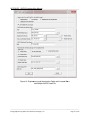
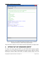
1
ACS SASSISASSI-ANSYS*
Integration Capability
Version 3.0
“Options A and AA”
An Advanced Computational
Software for 3D Dynamic
Analysis Including
Soil--Structure Interaction
Soil
User Manual
Revision 0
July 31, 2014
Ghiocel Predictive Technologies, Inc.
4 South Main St., 3rd Floor, Pittsford, NY 14534, USA
Phone: (585) 641641-0379/ Fax: (585) 586
586--4672
E-mail: acs.sassi@ghiocel
[email protected]
* ANSYS is a trademark of ANSYS, Inc.
DISCLAIMER
GHIOCEL PREDICTIVE TECHNOLOGIES, INC. DOES NOT W ARRANT THE
OPERATION OF THE ACS SASSI VERSION 3.0 PROGRAM W ILL BE
UNINTERUPTED OR ERROR-FREE. GHIOCEL PREDICTIVE TECHNOLOGIES, INC.
MAKES NO REPRESENTATIONS OR W ARRANTIES, EXPRESS OR IMPLIED,
INCLUDING, BUT NOT LIMITED TO, THE IMPLIED W ARRANTIES OF
MERCHANTIBILITY AND FITNESS FOR A PARTICULAR PURPOSE. Ghiocel
Predictive Technologies, Inc., in any case shall not be liable for any costs, damages,
fees, or other liability, nor for any direct, indirect, special, incidental, or consequential
damages (including loss of profits) with respect to any claim by LICENSEE or any third
party on account of or arising from this License Agreement or use the ACS SASSI
Version 3.0 program.
The ACS SASSI Version 3.0 baseline code using the standard skyline solver has been
extensively verified, tested, and used for seismic 3D soil-structure interaction models up
to 25,000 nodes including up to 5,000 interaction nodes. However, for 20,000 node or
slightly larger-size SSI problems, the standard solver becomes numerically inefficient
on typical PCs with 16GB RAM, since the SSI analysis runtime and the disk storage go
up out of hand.
The ACS SASSI Version 3.0 fast-solver code, called Option FS, has been extensively
verified, tested, and used for coherent seismic 3D SSI models up to 100,000 nodes
including up to 35,000 interaction nodes. The fast-solver code is much more
numerically efficient than the standard solver code. The ACS SASSI Version 3.0 fastsolver code has two major SSI problem size limitations for current MS Windows PC
platforms: 1) MS Windows OS limitation: The maximum accessed RAM for the SSI
problem is limited to 192 GB RAM for Windows 7 and 512 GB RAM for Windows 8,
respectively, and 2) ACS SASSI limitation: The total node number should be less than
100,000. The governing limitation of the SSI problem size is due to the MS Windows
OS limitation. On MS Windows PCs with 16 GB RAM, SSI problems with sizes up to
100,000 nodes including up to 8,000 interaction nodes can be run efficiently with the
fast-solver using the in-core SSI solution algoritm. For the SSI problems including
larger-size models with more than 80,000 nodes and 8,000-25,000 interaction nodes,
MS Windows PCs with RAM ranging from 32 GB up to 192 GB are recommended. For
large-size SSI problems with more than 20,000-30,000 interaction nodes, MS Windows
8 PCs with up to 512 GB RAM are recommended.
The fast-solver code is limited to arbitrary 3D SSI models. It does not work for 2D
models and 3D models with symmetry or antisymmetry conditions.
© Copyright 2014 by Ghiocel Predictive Technologies, Inc.
ACS SASSI - ANSYS Interface User Manual_________________________________________
Table of Contents
1. INTRODUCTION ...................................................................................................... 1
2. USING THE SUBMODELER MODULE FOR ACS SASSI AND ANSYS FE
MODELING ..................................................................................................................... 1
2.1. SUBMODELER Converters for ANSYS Models................................................ 2
2.2. SUBMODELER Commands for Checking and Building Complex SSI FEA
Models ......................................................................................................................... 4
3. OPTION “A” OR “ANSYS” ........................................................................................ 9
3.1. SSI Modeling Issues ....................................................................................... 12
3.2. Validation off the Two-Step Stress SSI Analysis ............................................. 13
3.3. SSI Methodology for Two-Step Approach ....................................................... 13
3.3.1. ANSYS Equivalent-Static Structural Stress SSI Analyses ......................... 15
3.3.2. ANSYS Dynamic Structural Stress SSI Analyses ...................................... 17
3.3.3. ANSYS Equivalent-Static Seismic Soil Pressure SSI Analyses................. 18
3.4. ACS SASSI-ANSYS Interface Description and Use........................................ 19
3.4.1. Requirements and Limitations ................................................................... 20
3.4.2. ACS SASSI-ANSYS Interface Description................................................. 21
3.4.3. ANSYS Seismic Load Generator for Exporting ACS SASSI SSI Responses
as Input Boundary Conditions to ANSYS Model (LOADGEN Module) ................... 24
3.5. ANSYS Equivalent-Static Analysis for Foundation Soil Pressures.................. 51
3.5.1. Linear Analysis Steps ................................................................................ 51
3.5.2. Nonlinear Analysis Steps ........................................................................... 51
3.5.3. Automatic Generation of the Surrounding Soil Deposit ............................. 53
4. OPTION “AA” OR “ADVANCED ANSYS” ............................................................... 54
4.1. ANSYS APDL Procedure to Generate Structural Matrices ............................. 56
4.2. Using SUBMODELER to Generate the HOUSEFSA Input File....................... 58
4.2.1. Surface SSI Models ................................................................................... 59
4.2.2. Embedded SSI Models .............................................................................. 60
4.3. Running the HOUSEFSA Module ................................................................... 62
_____________________________________________________________________________________________
© Copyright 2014 by Ghiocel Predictive Technologies, Inc.
i
ACS SASSI - ANSYS Interface User Manual_________________________________________
1.
INTRODUCTION
The ACS SASSI-ANSYS interfacing capability provides an advanced two-step SSI approach
that is capable of including more refined FEA structural models, local nonlinear material, and/or
nonlinear geometric aspects within the structure or at foundation interface with the soil. There
are two ACS SASSI-ANSYS interfacing options: i) Option A or ANSYS, and ii) Option AA or
Advanced ANSYS. Three demo problems, Demo 5, 6 and 7, are provided to help users
understand how to best use the ACS SASSI-ANSYS interface via Options A and AA.
The Option A or Option ANSYS of the ACS SASSI-ANSYS interfacing capability is based on an
integrated two-step SSI approach in which the 1st step is the overall SSI or SSSI analysis using
ACS SASSI and the 2nd step is the detailed structural stress analysis using ANSYS with the
input boundary conditions defined by the SSI responses computed with ACS SASSI. The
LOADGEN module (that is a part of the ACS SASSI MAIN module GUI) is used to transfer the
data from the ACS SASSI results database to the ANSYS input files.
Option A works with both the standard solver and the fast-solver implementations.
The Option AA or Option Advanced ANSYS of the ACS SASSI-ANSYS integration capability
consists of using directly an ANSYS structural model for SSI analysis without the need for
converting the structural model to ACS SASSI. The ANSYS structural stiffness, mass and
damping matrices are used directly by ACS SASSI for SSI analysis. The SSI relative
displacements, absolute accelerations and response spectra computed for the ANSYS
structural FEA model are obtained using the ACS SASSI software. The Option A should be
used to transfer the SSI response motions at all time steps or selected critical steps as input
boundary conditions for the ANSYS superstructure model only for computing structural stresses.
Option AA works with the fast-solver implementation only.
2.
USING THE SUBMODELER MODULE FOR ACS
SASSI AND ANSYS FE MODELING
The SUBMODELER module has similar functionalities to the PREP module, except the
graphical capabilities which are not in SUBMODELER. In addition to the PREP commands,
SUBMODELER has many new commands to check FE modeling and generate both the ANSYS
and ACS SASSI models, and also convert them back and forth, as needed by the user.
NOTE: The fact that SUBMODELER duplicates some of the PREP functionalities is due to our
intention to replace the PREP module by the SUBMODELER module in the future. The new
coming PREP based on the SUBMODELER module will have many additional pre- and postprocessing capabilities than the present PREP module.
_____________________________________________________________________________________________
© Copyright 2014 by Ghiocel Predictive Technologies, Inc.
Page 1 of 62
ACS SASSI - ANSYS Interface User Manual_________________________________________
SUBMODELER can use all the PREP commands used for building SSI models or selecting SSI
analysis options, including the AFWRITE command. The SUBMODELER also includes new
powerful commands for handling and combining multiple ACS SASSI or ANSYS models as
described in this section. The SUBMODELER is deficient in comparison with the PREP module
only on the graphical processing aspects, since it has no graphical capabilities at this time.
SUBMODELER can be launched by selecting RUN “ANSYS Soil Model Generator” from the
ACS SASSI MAIN menu.
As shown in the next sections, SUBMODELER is used in Option A to create the surrounding
soil deposit ANSYS model, or convert ACS SASSI models to ANSYS or vice-versa, and in
Option AA to transfer ANSYS model information to ACS SASSI to perform the SSI analysis
using the ANSYS structural model directly with no need for conversion to ACS SASSI.
2.1. SUBMODELER Converters for ANSYS Models
The SUBMODELER also has a powerful capability to convert models from ANSYS (.cdb file) to
ACS SASSI models. The SUBMODELER Converter has much fewer limitations than the MAIN
Converter. The ANSYS model conversion limitations for MAIN Converter are described in the
MAIN User Manual. In this section, only the SUBMODELER Converter limitations are described.
The SUBMODELER Converter is capable of converting ANSYS Version 13-14 models that
might have element types that are not fully compatible with the ACS SASSI element types. The
SUMBMODELER Converter can handle the following element types: i) SOLID element types;
SOLID45 and SOLID185, ii) SHELL element types; SHELL63 and SHELL181, iv) BEAM
element types; BEAM44 and BEAM188, v) PIPE element types; vi) COMBIN element types;
COMBIN14, vii) viii) Couple nodes (CP command) and ix) Constraint equations (CE commands)
and x) Multipoint constraint element types; MPC184: Rigid Link and/or Rigid Beam.
For ANSYS models with elements that are compatible with ACS SASSI, such as BEAM4,
BEAM44, SOLID45, SHELL63, COMBIN14 and MASS21, the SUBMODELER Converter has
the same limitations as the MAIN Converter with the exception that it can handle inputs from the
ANSYS Versions 13-14 models, and therefore, it is not limited to ANSYS Versions 11-12 as the
MAIN Converter is.
The SUBMODELER Converter limitations are described below.
The Material Data must be defined using the MPDATA command unless otherwise specified.
Any other way of defining this data is not recognized by the Converter.
The BEAM4/BEAM44 elements are convertible with some limitations: These beams must be
defined with the K node definition. These beams must have properties defined by the RBLOCK,
_____________________________________________________________________________________________
© Copyright 2014 by Ghiocel Predictive Technologies, Inc.
Page 2 of 62
ACS SASSI - ANSYS Interface User Manual_________________________________________
and the RBLOCK entry for the property must have 6, 8, 10, 12 or 19-24 fields for this element to
be converted properly. The end releases are defined by KEYOPT 6 and 7. The cross-section
commands are limited to SECTYPE, SECBLOCK and SECDATA.
The BEAM188 and PIPE288 elements are convertible with the following limitations. Pipes are
converted to equivalent beams only for visual simulation. These elements must be defined with
a K node definition.
WARNING: End releases for these elements cannot be defined for these beams because
ANSYS ENDRELEASE command creates new nodes and couples these nodes to simulate an
end release. This cannot be properly represented in ACS SASSI. The beam properties must be
defined by using the section commands. Beams must be defined with the ASEC or RECT type
option to be convertible. Section Offset must be default or not specified for beams (CENT is
default for beam) and must not be specified for pipes.
The COMBIN14 spring element with selected options is equivalent with the ACS SASSI
SPRING element type. COMBIN14 is convertible with the following limitations: KEYOPT 2 or
KEYOPT 3 must be defined for the group. KEYOPT 2 will take precedence if both KEYOPT 2
and KEYOPT 3 are defined. The spring constant must be defined by the by RBLOCK entry.
KEYOPT 2 options 1-6 are supported and options 1-2 for KEYOPT 3.
The MASS21 elements are equivalent with nodal masses defined in ACS SASSI. Mass data
must be defined in the RBLOCK entry.
The SHELL63 is equivalent to the ACS SASSI SHELL element type. The SHELL thickness must
be defined by RBLOCK entry. The SHELL181 is also convertible for visual simulation only with
the limitation that the shell thickness must be defined using section commands. The crosssection commands are limited to SECTYPE, SECBLOCK and SECDATA.
The SOLID45 is equivalent to the ACS SASSI SOLID element type. The SOLID185 is also
convertible for visual simulation with the limitation that KEYOPT4 which sets the option for
nonuniform materials is not defined or set to 0.
The SUBMODELER menu also includes the “Export to ANSYS” menu option that has an
identical functionality with the ANSYS command. The active model in the SUBMODELER is
exported in the ANSYS Versions 11-12 APDL format when this option is used.
WARNING: The conversion from ACS SASSI to ANSYS is problematic for BEAM44 when the
BEAM end releases are different from beam element to beam element inside of the group of the
BEAM elements. This is because ANSYS does not accept variations in beam releases from
element to element for the same ETYPE command that is equivalent to ACS SASSI Group
commands. In this case the structure of the ACS SASSI model and ANSYS model are not
compatible. For these situations we suggest use of the ANSYSREFORMAT command that
_____________________________________________________________________________________________
© Copyright 2014 by Ghiocel Predictive Technologies, Inc.
Page 3 of 62
ACS SASSI - ANSYS Interface User Manual_________________________________________
regroups all the beam elements into groups that have a common set of end releases and
creates a new ACS SASSI model that is compatible with ANSYS model.
WARNING: The SUBMODELER Converter will convert the ANSYS model in ACS SASSI format
so that it can be displayed in the PREP, but this model will be flagged by SUBMODELER and
the .hou file that the AFWRITE command generates will not be runnable using the standard
HOUSE module. If the SSI model isn't runnable with standard HOUSE module, the user will
receive a warning when the file is converted. The list of elements types below are the additional
element types that can be converted in the ACS SASSI PREP format for graphical processing.
There are no limitations on these elements because only element node connections need to be
translated for display.
The list below specifies the element type from ANSYS and the element type used to represent it
in the ACS SASSI model:
-
TRUSS180 will be displayed as a beam
MPC184 will be displayed as a Spring
PIPE16 will be displayed as a Beam
PIPE18 will be displayed as a Beam
Other elements will be ignored by the SUBMODELER Converter and not be included in the
model.
To run the SSI analysis for these converted ANSYS models that have different element types
than the ACS SASSI element types, a new, modified HOUSE module called HOUSEFSA is
required. This HOUSEFSA module is a part of the Option AA capability that is described in
Section 4.
2.2. SUBMODELER Commands for Checking and Building Complex
SSI FEA Models
In addition to the PREP commands for building FE models, SUBMODELER has many additional
commands for checking and building FE models which are described here, as follows:
INPUT, <filename> - This command provides the same functionality as the menu path File>Input used for loading an input text file. The input file name should include the full path, unless
the model name and path have been specified using the MDL command.
ACTM, <N> - The ACTM command switches the active model to the Model number N. The
initial Model number when SUBMODELER is started is 0. N can be any integer number.
MDL, <filename>,<path> - Create the path for the active Model. The path and model name will
also be used to define the path and file name used by the WRITE and ANSYS commands
_____________________________________________________________________________________________
© Copyright 2014 by Ghiocel Predictive Technologies, Inc.
Page 4 of 62
ACS SASSI - ANSYS Interface User Manual_________________________________________
DMODEL, <N> - Delete the FE model number N.
ANSYS, <filename>,<path> - The ANSYS command writes the model in an ANSYS APDL
input file (extension .inp). ANSYS, <filename>,<path> must be used if the active model name
and path have not yet been specified using the MDL command. If the model name and path
have been defined, then no arguments are necessary, and the ADPL file will be saved to the
active model directory
WRITE,<filename>,<path> - The WRITE command writes the model in an ACS SASSI PREP
input file (extension .pre). WRITE,<filename>,<path> must be used if the active model name
and path have not yet been specified using the MDL command. If the model name and path
have been defined, then no arguments are necessary, and the ADPL file will be saved to the
active model directory
For building SSI models:
ANSYSREFORMAT,<Org>,<Map> creates an ACS SASSI model input that has beam end
releases compatible with ANSYS model input structure. This command takes an ACS SASSI
model and regroups the beam elements based on their set of end releases, so that the beam
end releases can be translated into an ANSYS ADPL format correctly. This command should be
used with an empty active model. The user specifies which model should to be converted.
< Org> – Model number of the model to be reformatted
<Map> - A mapping file that indicates the correspondence between the original and the new
beam groups
SOILMESH, <Model>,<Scale X>,<Scale Y>, <Hori>, <Vert>,<mX>, <mY>,
<Thick>,<Contact> ,<RC num> - The SOILMESH command creates a soil FE mesh for the
active model and stores the model data in the user specified Model.
<Model>- user specified integer model number.
<Scale X> - percentage of growth in the X direction of each level, i.e. 0.07
<Scale Y> - percentage of growth in the Y direction of each level, i.e. 0.07
<Hori> - number of horizontal levels to build away from the embedment.
<Vert> - number of vertical levels to build away from the embedment.
<mX> - Centroid correction in the X direction
<mY> - Centroid correction in the Y direction
<Thick> - Thickness of each new level.
<Contact> - if equal 0 do not use contact surfaces, else include contact surfaces in the
model.
<RC num> - defines the constant set number to be used in ANSYS for the contact
surface Real Constants
_____________________________________________________________________________________________
© Copyright 2014 by Ghiocel Predictive Technologies, Inc.
Page 5 of 62
ACS SASSI - ANSYS Interface User Manual_________________________________________
WARNING: If the excavation volume has lateral walls that are not vertical, or if the node layers
are different at different excavation levels, then SOILMESH will not work correctly.
EXCAV,<model>,[delta] - This command creates an excavation volume model for a SSI model
that doesn't have an excavation volume. The command will use the lowest vertical z-level grid
as a template to create a homogenous mesh model up to ground surface. The new excavation
model will be stored in the model ID number given by the user. The ground surface must be
defined properly in the model used in the generation. The delta parameter is a factor used to
match slight variations in z-level used in some models for the same embeddment level. Models
that don't have uniform z coordinates across the floor should use a delta > 0, so that the
command doesn't generate multiple levels for the small variations of Z.
<model> – Model ID number to store the new excavation volume
[delta] - allowable distance of z-level variation on a single level (Default = 0). Parameter
delta should be entered as a positive floating point number or the default will be used.
WARNING: If there are outcropping beneath ground surface that do not extend to the bottom zlevel the code will not generate excavation volume for these areas.
MERGESOIL,<Struct>,<Soil>,[Mode],[StiffStiff],[StiffSoft],[SepLevel],[Mapping] – This
command is used to merge the structural and the excavation volume models together in a new
active SSI FEA model.
<Struct> - Model Number of the Structure
<Soil> - Model Number of the Excavation volume
[Mode] - merging nodes on the structure excavation interface
= 0 unbonded lateral foundation-soil interface with side solid
= 1 bonded lateral foundation-soil interface (default)
= 2 bonded foundation-soil interface using duplicate nodes connected by stiff springs
= 3 unbonded foundation soil-interface using duplicate nodes connected by soft springs
[StiffStiff] - Stiff spring stiffness for Modes 2 and 4. (Default = 10^7)
[StiffSoft] - Soft spring stiffness for Modes 3. (Default = 10)
[SepLevel] - Global z-coordinate level for the depth where soil separation occurs
[Mapping] - This is mapping filename for the duplicate node merging
GROUNDELEV,<elev> - This command sets the ground elevation constant for the SSI model.
This is constant is also set by the HOUSE command.
<elev> - The ground elevation for the model.
GRAVITY,<grav> - This command sets the gravity constant for the model. This is constant is
also set by the HOUSE command.
<grav> - The gravity constant for the model.
NCOM - This command compresses the node list so there are no gaps in the defined node
numbering in the current model. The command also updates the node element connections in
the model to reflect the new node numbering in the model. The command will maintain relative
order of the nodes in the model.
_____________________________________________________________________________________________
© Copyright 2014 by Ghiocel Predictive Technologies, Inc.
Page 6 of 62
ACS SASSI - ANSYS Interface User Manual_________________________________________
GCOM - The GCOM command will compress group number so there are no gaps in the group
numbering. The new group numbering will start a 1. The relative order of the groups will not
change and this command does nothing to compress the element numbers in each group (use
ECOMPR to element numbers inside of groups).
RMVUNUSED – The RMVUNUSED Command checks elements and interaction nodes in the
current model to see which nodes are being used. All unused, non interaction nodes will be
removed from the model. This command does not compress node numbers or change element
node connections. The command should be used in conjunction with NCOM to compress the
node list of a complete model.
INTGEN,<type>,[skip] - automatically generates interaction nodes for different substructuring
approaches FV, FI-FSIN (SM), FI-EVBN (MSM), Surface model and Fast FV . The excavation
volume must be explicitly defined by the ETYPE command for options 1-3. If the ETYPE of the
elements is left to the default values, this command will not work. The <type> argument is the
type of iteration node generation to be used:
=1
=2
=3
=4
=5
Embedded Foundation - Flexible Volume (FV)
Embedded Foundation - Flexible Interface with Excavation Volume Boundary Nodes,
denoted FI-EVBN or Modified Subtraction Method (MSM)
Embedded Foundation - Flexible Interface with Foundation-Soil Interface Nodes,
denoted FI-FSIN or Subtraction Method (SM)
Surface Foundation (interaction nodes are only at the ground surface level)
Embedded Foundation - Fast FV including multiple layers of internal interaction nodes
The [skip] argument is only necessary when using type 5. Type 5 gives the option to include
intermediate layers of interaction nodes between the surface and bottom of the foundation. The
[skip] argument specifies the number of node layers to be skipped before generating the next
layer of interaction nodes. For example, setting the [skip] argument to 1 will result in interaction
nodes being generated at every other level of nodes in the excavation volume.
ETYPEGEN,<type> - assigns the type of SOLID elements. These SOLID elements can be
either a part of the structure or a part of the excavation volume based on ETYPE. The type is
implicitly defined by default (ETYPE = 0) when an element is added. Then, during AFWRITE
rules are used to determine if implicitly defined elements are structural or excavation *.hou file.
However, when using WRITE file the implicit ETYPE definition is maintained in the *.pre file.
Some INTGEN options require explicitly defined types of elements to work correctly. Use
ETYPEGEN,<type> to either explicitly type elements using the AFWRITE rules, or changes the
type of all the elements in the model. Depending on the assigned value, the type parameter has
the following functionalities:
=0
changes all implicitly defined element type to explicitly defined element type
_____________________________________________________________________________________________
© Copyright 2014 by Ghiocel Predictive Technologies, Inc.
Page 7 of 62
ACS SASSI - ANSYS Interface User Manual_________________________________________
=1
=2
sets all elements to structural
sets all elements to soil
For checking SSI models:
FIXEDINT checks SSI model to find if there is any fixed interaction node (that is a SSI modeling
error). No parameter is needed.
HINGED checks model to find all hinged connections between solids and shell and beams and
beams and shells. These hinged connections could indicate potentially incorrect FE modeling,
since the node rotations from beams and shells are not transmitted to solids at the common
nodes, and the node rotations from beams are not transmitted the in-plane shell rotations at the
common nodes (the drilling dof equations have no stiffness terms by default).
KINT - The command will check the K-nodes of all Beams to see if they are also defined as
interaction nodes. K nodes that are interaction nodes may cause incorrect simulation results.
This command will report the nodes that have this issue to the user and remove the node from
interaction node list.
FREESPRING - This command will find all unconstrained node dofs that are only connected to
a spring, and warn the user about this condition at the nodes where it occurs.
For improving SSI models:
FIXROT,<Stiff> - automatically fixes the unnecessary rotational degrees of freedom and adds
soft rotational springs to improve numerical conditioning for shell models (for the Kirckhoff plate
element the drilling degree of freedom has no stiffness associated with it, and therefore could
produce poorly conditioned or unstable numerical models). Using FIXROT,<Stiff> will fix all
rotational dofs for nodes that belong only to solid elements or shell elements that are parallel to
global system planes and have no connection that provides stiffness for the shell in-plane
rotations. The FIXROT command fixes rotations by using the D command to fix rotations
described above.
For the shell elements that are not parallel to a global coordinate system planes, the FIXROT
command automatically adds low-stiffness in-plane rotational springs to each node of the shells
(rotations around the normal to the shell planes). The user can control the rotational spring
stiffness using the <stiff> parameter of the command. By default the rotational spring stiffness is
10. The user can change the <stiff> parameter values in the updated .pre file as needed if more
or less local stiffness is desired in particular sections of the model. To do this, the user should
edit the values of the “SC” commands in the .pre file. The stiff parameter = 10 is an appropriate
value for typical nuclear structure models that consist of concrete shells for which the shell
bending stiffnesses are at least several thousand times larger if defined in kips-ft/rad. The
recommendation based on FE theory is that the stiff parameter should be less than 10% of the
_____________________________________________________________________________________________
© Copyright 2014 by Ghiocel Predictive Technologies, Inc.
Page 8 of 62
ACS SASSI - ANSYS Interface User Manual_________________________________________
shell element bending stiffness. The user will need to use the WRITE command to save all the
FIXROT command fixes in an updated .pre input file that then can be reviewed by the user.
FIXSLDROT - This command fixes the rotational degrees of freedom of all the nodes that are
only connected to Solid elements.
FIXSPRROT - This command fixes the rotational degrees of freedom of all the nodes that are
only connected to Springs and Springs/Solid node connections. If the node is only connected to
a Spring the unconstrained degrees of freedom are determined by the spring stiffness. If the
node is connected to Springs and Solids the rotational degrees of freedom are determined by
the Springs rotational stiffness.
FIXSHLROT,<Stiff> - This command applies rotational soft springs to all nodes that are only
connected to coplanar shells. The overall spring stiffness is determined by the stiffness
argument of the command and applied along the normal shell's plane.
<stiff> – Stiffness of the soft springs added to shells to remove the shell drilling rotation
singularities (default stiffness value is 10)
WARNING: The above FIXROT and FIXSHLROT commands are HIGHLY RECOMMENDED to
be used for ACS SASSI FE shell models that have shells that are oblique with respect to the
global coordinate system planes. These oblique shell elements can produce numerically
unstable SSI models. The use of FIXROT/FIXSHLROT ensures that no numerical singularities
could be produced by the shell drilling equations. The use of FIXROT/FIXSHLROT is highly
recommended especially if large-size SSI models are run with the fast-solver SSI modules
(HOUSEFS and ANALYSFS) are used. Benchmark results obtained against ANSYS for various
fixed-base models have indicated that the use of the FIXROT/FIXSHLROT commands is highly
beneficial for improving numerical condition of the FEA shell models. The use of
FIXROT/FIXSHLROT makes the two FEA codes provide same results for the identical
configuration shell models (using SHELL63 in ANSYS to be consistent with the ACS SASSI
Kirckhoff thin plate element formulation). The use of FIXROT/FIXSHLROT has no improving
effects when the ANSYS FE shell models are used directly via the Option AA capability.
3.
OPTION “A” OR “ANSYS”
The “Option A” or “Option ANSYS” ACS SASSI-ANSYS interfacing capability is based on an
integrated two-step SSI approach in which the 1st step is the overall SSI or SSSI analysis using
the ACS SASSI model and the 2nd step is the detailed structural stress analysis using the
ANSYS model with the input boundary conditions defined by the SSI responses. The
LOADGEN module (that is a part of the ACS SASSI MAIN module GUI) is used to automatically
transfer the data from the ACS SASSI result database to the ANSYS input files.
The 2nd step using ANSYS has two distinct functionalities:
i) perform structural stress analysis using refined ANSYS FE structural models with
detailed meshes, eventually including enhanced element types, non-linear material and
plasticity effects, contact and gap elements, and
_____________________________________________________________________________________________
© Copyright 2014 by Ghiocel Predictive Technologies, Inc.
Page 9 of 62
ACS SASSI - ANSYS Interface User Manual_________________________________________
ii) compute seismic soil pressure on basement walls and slabs including soil material
plasticity, foundation soil separation and sliding using refined ANSYS FE soil deposit models.
The 1st functionality involves creating a more “detailed” FE model in ANSYS that corresponds
to the “coarse” ACS SASSI structural model, while the second functionality implies creating an
FE submodel of the surrounding soil deposit in ANSYS. Figures 1 and 2 show the new ANSYS
FE models created by the ACS SASSI-ANSYS interfacing tools that correspond to the two
functionalities mentioned above. It should be noted that the two-step SSI analysis is based on a
“cascaded” analysis assumption in which the SSI responses output from the first step (ACS
SASSI SSI analysis) becomes the input boundary conditions for the second step (ANSYS stress
analysis). In the second step of ANSYS analysis, local nonlinear material or geometric aspects
can be considered. The “cascaded” assumption implies that there is no feedback effect due to
the local structural and foundation nonlinearities on the SSI soil motions at the foundation-soil
interface. This assumption appears to be reasonable for practical applications, except for some
particular situations when the foundation separation from the surrounding soil is quite large.
The Option A two distinct functionalities are handled by three separate software modules, the
Converter module, the LOADGEN module and the SUBMODELER module. The LOADGEN and
SUBMODELER modules are two standalone modules, while the Converter module is part of the
SUBMODELER module. It should be noted that in addition to the Converter included in the
SUBMODELER, there is another standalone Converter module that is included in the MAIN
module menu. This older Converter is still available, but has fewer capabilities than the newer
Converter included in the SUBMODELER module. The key difference is that the MAIN
standalone Converter module is limited to the ANSYS Versions 11 and 12, while the
SUBMODELER Converter can translate models from the ANSYS Versions 13 and 14 in addition
to the ANSYS Versions 11 and 12.
The Converter module translates the ANSYS models saved in the .cdb input format into ACS
SASSI structural models in the PREP or SUBMODELER .pre input format, or vice versa
translate the ACS SASSI models in the .pre format into ANSYS structural models in the APDL
input format. In the latter case, the ACS SASSI excavation volume part of the embedded SSI
models is automatically deleted during the conversion to the ANSYS model. The model
conversions are done efficiently via the command line in SUBMODELER.
_____________________________________________________________________________________________
© Copyright 2014 by Ghiocel Predictive Technologies, Inc.
Page 10 of 62
ACS SASSI - ANSYS Interface User Manual_________________________________________
Figure 1 Coarse Model (identical to SSI structural model) vs. Detailed Model (user defined)
Figure 2 Surrounding Soil ANSYS Model Generated by ACS SASSI SUBMODELER Module
_____________________________________________________________________________________________
© Copyright 2014 by Ghiocel Predictive Technologies, Inc.
Page 11 of 62
ACS SASSI - ANSYS Interface User Manual_________________________________________
The LOADGEN module uses a simple GUI window dialog to transfer the seismic SSI boundary
conditions, the seismic loading, and relative displacements at the foundation soil interface from
the ACS SASSI SSI result database (.acc and .thd frames) to the ANSYS structural model via a
ANSYS APDL command file. This can be done either for a single time step, or all time steps, or
selected critical time steps.
The SUBMODELER module, similar to the LOADGEN module, uses a simple GUI window
dialog to generate a new surrounding soil FE submodel in the ANSYS APDL input format,
based on the ACS SASSI SSI model embedment geometry. The LOADGEN module is then
used to transfer the SSI relative displacements at the interaction nodes defined at the
foundation interface with respect to the free-field motion, and the nodal seismic forces for all
active dofs at the selected time steps.
3.1. SSI Modeling Issues
The second step analysis performed in ANSYS can be either i) a quasi-static or equivalent static
stress analysis performed for the selected critical time steps, or ii) a dynamic stress analysis
using the direct integration approach
The ANSYS equivalent-static analysis option is applied at all or selected critical time steps, so
that the seismic loading phasing and foundation deformations are correctly included. It should
be noted that the ACS SASSI-ANSYS equivalent-static stress analyses at selected time steps
are more accurate than those computed using the traditional “ZPA-based approach” that
computes the seismic equivalent-static forces based structural the ZPA values. However, for the
users’ convenience, the traditional ZPA-based approach can be also applied using the ACS
SASSI-ANSYS interfacing capability.
For seismic soil pressure SSI analyses, both the LOADGEN and SUBMODELER modules are
used, as explained in this manual. Both linear elastic analyses and nonlinear equivalent-static
analyses, including nonlinear soil and foundation-soil separation effects can be considered.
The ANSYS dynamic time-domain direct integration analysis uses all time steps. The major
benefit of the time-domain dynamic ANSYS analysis is that is greatly reduces the computational
requirements of a direct ANSYS SSI analysis approach by eliminating the need of including
additional surrounding soil elements for large distances in the structural FE model. Instead, the
SSI boundary conditions corresponding to the SSI foundation relative displacements with
respect to the free-field motion are applied at the foundation-soil interface nodes, and the
kinematic SSI seismic loads are applied to structure. These SSI relative displacements that are
applied at the foundation-soil interface nodes should be computed at the different embedment
depth levels by the difference between the foundation SSI motion and the free-field motion at
the same depth.
_____________________________________________________________________________________________
© Copyright 2014 by Ghiocel Predictive Technologies, Inc.
Page 12 of 62
ACS SASSI - ANSYS Interface User Manual_________________________________________
It should be noted that ANSYS direct integration approach is limited in practice to the Rayleigh
damping matrix option that assumes that structural damping is frequency-dependent. This is a
significant modeling limitation, since for the structural and soil hysteretic materials the damping
is independent of frequency, so that the Rayleigh damping can be too crude. The use of the
frequency-dependent Rayleigh damping could significantly overdamp the low and the high
frequency structural responses. Also, ACS SASSI uses a structural mass matrix that is a mixed
lumped and consistent mass matrix, while ANSYS uses either a lumped mass matrix or a
consistent matrix for the direct time-domain integration approach. Thus, some visible differences
between the ACS SASSI dynamic response and the ANSYS dynamic response are expected.
3.2. Validation off the Two-Step Stress SSI Analysis
The high computational accuracy of the implemented ACS SASSI-ANSYS dynamic and
equivalent-static SSI stress approaches are demonstrated in the Verification Manual, Problem
32. This problem includes comparisons of the ACS SASSI and ANSYS displacements and
stress results for the fixed-base model, the surface SSI model, and the deeply embedded SSI
model.
It should be noted that for the quasi-static (or equivalent-static) analysis, the ANSYS structural
stresses and the ACS SASSI structural stresses matching is practically perfect for identical
structural FEA models, i.e. when the ANSYS model is obtained using the ACS SASSI automatic
converters. However, for the ANSYS dynamic SSI analysis option, the ANSYS and ACS SASSI
stresses could be significantly different due to the fact that the mass and damping matrices are
different, and the numerical algorithms are different.
WARNING: If the ANSYS dynamic SSI analysis option is selected, then, the differences
between ANSYS and ACS SASSI SSI results due to different mass and damping matrix
formulations, and numerical solution methods, as the direct time-integration integration method
in ANSYS and the complex frequency convolution method in ACS SASSI, have to be evaluated
by the user before the final SSI production runs are started.
WARNING: For embedded structures, the user should compute kinematic SSI structural
accelerations (for zero mass structure) and then use them to define the translational and
rotational rigid-body acceleration fields, as required to define the seismic load forcing function
inputs for the ANSYS dynamic analysis. In addition, the foundation relative displacements with
respect to the free-field motions shall be computed for all the excavation levels.
3.3. SSI Methodology for Two-Step Approach
Before using the ACS SASSI-ANSYS integration capability, the user must convert the ACS
SASSI structural model to an ANSYS structural model using the ACS SASSI converter. The
converter produces an ANSYS model that is identical with the ACS SASSI structural model.
This will be referred to in this documentation as the “Coarse ANSYS model”.
_____________________________________________________________________________________________
© Copyright 2014 by Ghiocel Predictive Technologies, Inc.
Page 13 of 62
ACS SASSI - ANSYS Interface User Manual_________________________________________
WARNING: The user has to make sure that this "Coarse ANSYS model" includes no "D" nodal
constrains. This is required since this ANSYS model will be used to generate the mass matrix
data via modal analysis option.
The Coarse ANSYS model (converted from ACS SASSI) can be used as a starting point for
building a Detailed ANSYS structural model by using either the EREFINE command for SHELL
models or other options in ANSYS.
The user can also develop a Detailed ANSYS structural model directly in ANSYS, not by using
the converted ACS SASSI model. The Detailed ANSYS does not need to have the node or
element numbering, or even the geometry configuration of the Coarse ANSYS model (that is
identical configuration with the SSI model). However, we recommend as a good practice to
include all the nodal points from the Coarse ANSYS model in the Detailed ANSYS model. The
seismic loads and relative displacements are transferred from ACS SASSI to ANSYS only
based on the node coordinate information, and the applied loads and BCs are placed at the
closest coordinate from the nodes in the Detailed ANSYS model.
The LOADGEN module ensures the automatic transfer of the SSI responses in terms of nodal
seismic forces (based on the node accelerations, computed with MOTION) and nodal relative
displacements with respect to free-field motion (computed with RELDISP) to the ANSYS model.
The seismic SSI boundary conditions (nodal seismic loads and/or nodal relative displacements)
from the ACS SASSI structural model are automatically transferred to the refined, Detailed
ANSYS structural. Foundation displacements can be also transferred to the surrounding soil
submodel. The nodal coordinates of the Coarse ANSYS model are used to identify the node
locations of the seismic loads and relative displacements in the Detailed ANSYS model.
For computing the seismic loads on the Detailed ANSYS model, user has two options:
i) use the lumped mass matrix of the Coarse ANSYS model, or
ii) use the reduced mass matrix obtained from the Detailed ANSYS model via the
ANSYS Guyan reduction for computing the structural seismic forces (nodal masses
multiplied by the nodal accelerations).
If the lumped mass matrix option i) is used, then the Coarse ANSYS model needs to be
generated using the SUBMODELER. If the reduced mass matrix option ii) is used, then, the
Detailed ANSYS model will be used directly for computing the reduced mass matrix data or the
master mass that corresponds to the node dofs of the Coarse ANSYS model The user must
make sure the Detailed ANSYS model includes no "D" node dof constrains.
_____________________________________________________________________________________________
© Copyright 2014 by Ghiocel Predictive Technologies, Inc.
Page 14 of 62
ACS SASSI - ANSYS Interface User Manual_________________________________________
3.3.1. ANSYS Equivalent-Static Structural Stress SSI Analyses
Three options for the ANSYS quasi-static or equivalent-static SSI are implemented. These three
options depend on the type of the seismic SSI responses used for the second step analysis:
i)
ii)
iii)
Accelerations for all structural dofs. This still needs “calibrated” soil springs at the
foundation support nodes,
Accelerations for all structural dofs and Displacements for the foundation-soil
interface nodes, and
Displacements for all structural dofs.
The last two of the above equivalent-static approaches are theoretically “exact” for identical
structural FE models in ACS SASSI and ANSYS. Figure 3 reviews the capabilities of the three
equivalent-static analysis approaches.
These equivalent-static approaches can use SSI seismic loads and/or displacements that are
transferred at each time step or at selected critical time steps. These critical time steps, tk, are
those for which maximum structural stresses/forces are reached in different parts of the
structure at different time steps. These critical time steps can be selected by the user using the
ACS SASSI PREP time-history visualization tools, or more efficiently by using the automatic
stress “peak” selection option in the ACS SASSI PREP Batch menu.
Using LOADGEN, the seismic load and foundation displacements at all or selected critical time
steps will be transferred automatically to ANSYS model in the APDL format in separate load
steps. The final stress results should be obtained by the user by enveloping the absolute value
results from different load steps.
WARNING: No output requests are included in the load step files. The output request is entirely
at the ANSYS user discretion and responsibility.
It should be noted that user is also able to select only a portion of the structure as a submodel
for further perform the detailed stress analysis. The Displacements and Acceleration options
could be combined, so that SSI relative displacements are transferred at the boundary nodes of
the submodel and the seismic forces are applied at the submodel interior nodes. In this case,
the user has to select all the structural nodes around the selected portion of the structure as
interaction nodes, so that LOADGEN will transfer the node relative displacements of these
nodes as SSI boundary conditions into the ANSYS APDL file.
It should be noted that the traditional ZPA-based approach that uses the SSI maximum nodal
acceleration response values to compute equivalent-static seismic forces could be applied in
conjunction with the above option i). However, the ZPA-based equivalent-static approach is
generally overly conservative, especially for non-symmetric structures, but, it can also be locally
unconservative, since it loses the phasings of the seismic loads on the structure. The ZPA_____________________________________________________________________________________________
© Copyright 2014 by Ghiocel Predictive Technologies, Inc.
Page 15 of 62
ACS SASSI - ANSYS Interface User Manua
Manual_________________________________________
_________________________________________
based approach requires that the user determin
determines
es calibrated soil springs that need to be
included at the foundation support nodes, or assume a rigid base. The rigid base assumption
could be very crude, especially for flexible foundations in soft soils as shown in the Problem 32
of the Verification Manual.
ANSYS Equivalent
Equivalent-Static
Static Structural Analysis: Using Acceleration Input
Figure 3 ACS SASSI-ANSYS
(left), Displacement Input (right) and Mixed, Acceleration and Displacement Inputs (middle)
Table 1 describes the different types of equivalent
equivalent-static stress
ss analysis that were implemented
based on the SSI approaches illustrated in Figure 3. Of these approaches, the mixed approach
using both the SSI acceleration and displacement boundary condition as inputs shown in the
middle of Figure 3 is recommended as tthe
he best approach. This approach is particularly useful,
when the ANSYS equivalent-static
static model is much more refined than the SSI model, and/or
when improved element types for computing stresses, and/or local structural nonlinearities are
included.
_____________________________________________________________________________________________
© Copyright 2014 by Ghiocel Predictive Technologies, Inc
Inc.
Page 16 of 62
ACS SASSI - ANSYS Interface User Manual_________________________________________
Table 1 ANSYS Equivalent-Static Seismic Stress Analyses Including SSI Effects
3.3.2. ANSYS Dynamic Structural Stress SSI Analyses
Through the ACS SASSI-ANSYS integration capability, ANSYS can be used to perform an
efficient dynamic analysis in the second analysis step using either the Coarse or the Detailed
ANSYS model. In this case, the seismic load is defined by the kinematic SSI forces on the
structure that are introduced by the SSI translational and rotational rigid-body acceleration
history of the massless structure. The foundation flexibility SSI effects are included at the
foundation-soil interface nodes through the relative displacement histories with respect to the
free-field input motions at different excavation levels.
WARNING: Due to the differences in the dynamic modeling in ANSYS and ACS SASSI, i.e.
different formulations for the mass and damping matrices, and different numerical techniques for
solving the differential equations of motion for SSI system, we recommend a preliminary
comparative ACS SASSI-ANSYS stress analysis using identical FEA models in the two codes,
i.e. the Coarse ANSYS model that is obtained by converting from the ACS SASSI model. Such
a preliminary comparison between Coarse ANSYS model results and ACS SASSI results is
necessary to validate the ANSYS dynamic model, including the Rayleigh damping modeling
_____________________________________________________________________________________________
© Copyright 2014 by Ghiocel Predictive Technologies, Inc.
Page 17 of 62
ACS SASSI - ANSYS Interface User Manual_________________________________________
against ACS SASSI results. After the ANSYS model validation is passed, only then, for the final
stress analyses, the Detailed ANSYS model can be used instead of the Coarse ANSYS model.
3.3.3. ANSYS Equivalent-Static Seismic Soil Pressure SSI Analyses
Using the ACS SASSI-ANSYS integration, the user can efficiently and accurately compute the
seismic soil pressure on the embedded foundation walls and base slabs. Using ANSYS
equivalent-static analysis, the seismic soil pressures can be computed for the critical time steps.
These critical time steps are usually those that produce the largest base shear, sliding forces
and overturning moments.
The first action taken by the user before performing the seismic soil pressure analysis is to
generate the ANSYS submodel for the surrounding soil deposit. This soil model is then used for
the soil pressure analysis. Using the SUBMODELER module the user can automatically
generate a surrounding soil deposit model full control over the mesh refinement and extension.
In general, for an equivalent-static stress analysis, the soil deposit should extend about twice
the size of the foundation to eliminate any effect the soil deposit boundaries away from the
foundation area may have on the soil pressure results. The user should perform some
sensitivity studies on the soil mesh sizes and its extension in lateral and vertical directions to
ensure that both are correctly sized for the problem.
NOTE: The user could use limited extension surrounding soil model with displacement
boundary conditions input from SSI analysis.
Two ACS SASSI-ANSYS equivalent-static approaches are implemented, as shown in Figure 4:
i) Linear Analysis (foundation is bonded with the elastic soil) uses as the SSI boundary
condition inputs the SSI foundation-soil interface node relative displacements with respect to the
free-field motion, and
ii) Nonlinear Analysis (foundation can separate from soil material that can behave linear
or nonlinear) uses as SSI boundary condition inputs the SSI seismic loads on the structure
including basement.
It should be noted that the Linear Analysis (LA) option requires only the use of the surrounding
soil deposit model with relative displacement boundary conditions. No structural model is
needed. The Nonlinear Analysis (NA) option requires the use of both of the ANSYS structural
and soil deposit models, with the SSI seismic loads transferred to the structure model.
Theoretically, the NA option can be also applied using the ANSYS dynamic time-integration
approach, but in this case the model size and the mesh refinement of the soil deposit is
dramatically larger to handle the high-frequency wave components transmission and the
reflected waves into the infinite soil media space. Inclusion of a large-size soil model will
_____________________________________________________________________________________________
© Copyright 2014 by Ghiocel Predictive Technologies, Inc.
Page 18 of 62
ACS SASSI - ANSYS Interface User Manual_________________________________________
produce huge computational analysis efforts and therefore, is totally impractical for seismic SSI
design-basis analyses.
If dynamic analysis is used, then, the user has to input the desired boundary conditions for the
ANSYS soil deposit model. By default, no boundary conditions are placed on the lateral
surfaces of the soil deposit model.
Figure 4 Seismic Soil Pressure Equivalent-Static SSI Analysis: Nonlinear/Linear Analysis Using
Seismic Loads (left) and Linear Analysis Using Support Displacements (right)
3.4. ACS SASSI-ANSYS Interface Description and Use
The ACS SASSI-ANSYS interface capability provides an efficient tool to perform the second
analysis step using a Detailed ANSYS model. The ACS SASSI-ANSYS interface tool
(LOADGEN module) automatically generates the SSI boundary condition input files for the
Detailed ANSYS model. The SSI boundary condition inputs consist of the nodal seismic forces
within the structure and/or nodal relative displacements at the foundation interface with
surrounding soil. The required SSI boundary conditions are automatically transferred to ANSYS
in an APDL format input file. This APDL file contains nodal forces and/or relative displacements
for ANSYS equivalent-static analyses, and nodal displacements and acceleration field data for
ANSYS dynamic analyses. The type of SSI boundary condition input is selected by the user
from the ACS SASSI SSI analysis result database.
_____________________________________________________________________________________________
© Copyright 2014 by Ghiocel Predictive Technologies, Inc.
Page 19 of 62
ACS SASSI - ANSYS Interface User Manual_________________________________________
It should be noted that the SSI nodal forces and nodal displacements are transmitted to the
ANSYS model based on the structure node coordinates. The nodal seismic load and/or relative
displacements with respect to the free-field control motion from the SSI analysis are applied at
the same node locations within the Detailed ANSYS model.
The nodal acceleration response data is converted to the nodal seismic forces by multiplying
them with nodal masses. The displacement boundary conditions and the seismic forces are
generated in the ANSYS APDL format input files, so that the user can apply them directly to
ANSYS using the command, “/INPUT, …”.
The user has two options for defining the nodal seismic forces for the Detailed ANSYS model
based on the mass matrix formulations:
1)
Lumped Mass matrix of the Coarse ANSYS model that is identical to the SSI model
(this ANSYS coarse model can be obtained by the user using the new ACS SASSI
PREP converter from ACS SASSI to ANSYS), and
2)
Reduced Mass matrix of the Detailed ANSYS model (using a Guyan reduction of the
mass matrix of the Detailed ANSYS model assuming as masters all the active
degrees of freedom of the Coarse ANSYS model.
3.4.1. Requirements and Limitations
In this section we describe the use of the ANSYS load generator or LOADGEN module
(included in the MAIN GUI menu) to transfer the ACS SASSI SSI analysis result data as input
boundary conditions for the ANSYS detailed stress analysis.
Before using the LOADGEN module options the user needs to make sure that the appropriate
SSI model and result database are used, since otherwise the LOADGEN module will not
function correctly. These must be open in MAIN when LOADGEN is launched. The current
database path and model name are shown in the bottom right of the MAIN window.
There are a few things the user needs to pay attention when using LOADGEN:
1) Avoid having coincident node locations. Avoid having nodes with the same coordinates.
The load generator uses the nodal coordinates from the SSI model to determine which
node in the Detailed ANSYS are loaded Therefore, if there are two or more nodes with
same coordinates, the ANSYS load generator cannot distinguish between these two
nodes. The coincident nodes will cause the displacements or inertial forces to potentially
be applied incorrectly. This incorrect load can cause erroneous results in the static
analysis. When there are coincident nodes in the ANSYS refined model, the user should
check if the displacement BC's and inertial forces are applied correctly.
2) When the “Lumped Mass” option is selected for the “Generate Mass Data” input using
the Coarse ANSYS model, the user must make sure the Coarse ANSYS model has no
_____________________________________________________________________________________________
© Copyright 2014 by Ghiocel Predictive Technologies, Inc.
Page 20 of 62
ACS SASSI - ANSYS Interface User Manual_________________________________________
displacement constraints (from the “D” command in ANSYS) at any node. Also, if there
are beam elements with end-released degrees of freedom in the Coarse ANSYS model,
the ANSYS model the nodal masses cannot be extracted, as these are not compatible
with the “LUMPM” option for modal analysis. Refer to section 3.4.3 for an explanation
on how to deal with this scenario.
3) When select the “Master Node Mass” option for the “Generate Mass Data” input using
the Detailed ANSYS model, the user has to make sure the Detailed ANSYS model has
no displacement constraints (from the “D” command in ANSYS) on the model. The
reason same as for above item 2).
WARNING: It is strongly advised to include all the nodes from the Coarse ANSYS model in the
Detailed ANSYS model. Since ANSYS will apply the nodal loads to the nodes of the Detailed
ANSYS model with the nearest coordinates to the Coarse ANSYS model nodes, it is
recommended that all the Coarse ANSYS model nodes to be included in the Detailed ANSYS
model to ensure that the loads are not applied to incorrect nodes. Failure to include coarse
model nodes with the same coordinates in the detailed model will require the user to extensively
check the detailed model to ensure that the loads from coarse model are applied to the correct
locations. This checking is a MUST when the detailed model has a different geometry
configuration and/or different element types than the coarse model. This applied load checking
is labor intensive and has significant associated risks. Also, as above mentioned, the existence
of pairs of duplicate nodes with the same coordinates should be avoided in both models since
they can generate the same problem of misplacing the nodal loads in the detailed model.
3.4.2. ACS SASSI-ANSYS Interface Description
The ACS SASSI-ANSYS integration modules, LOADGEN and SUBMODELER (or SOILMESH
in previous version), are accessible though the ACS SASSI MAIN module. After using the
SUBMODELER model converter to create a Coarse ANSYS structural model equivalent to the
ACS SASSI structural model, the user will transfer the seismic loads and displacements from
the SSI result database to ANSYS model with the LOADGEN module.
The ANSYS load generator (the LOADGEN module) provides four functions to convert the SSI
displacements and/or accelerations at all or selected critical time steps from the ACS SASSI
results into the ANSYS seismic load via APDL format input file, as shown in Figure 5.
The four options are organized in the first user input data group labeled as “Data to Add from
ACS SASSI to the ANSYS model"
1. “Displacements” option provides the function to apply displacements only;
2. “Acceleration” option provides the function to apply inertial forces only;
_____________________________________________________________________________________________
© Copyright 2014 by Ghiocel Predictive Technologies, Inc.
Page 21 of 62
ACS SASSI - ANSYS Interface User Manual_________________________________________
3. “Displacement and Acceleration” option provides the function to apply both
displacement boundary conditions and seismic forces from nodal accelerations which
here will be referred to as a “mixed” boundary condition;
4. “Displacement for Soil model” option provides the function to generate the
displacement boundary conditions for soil FE model that is used to compute the seismic
soil pressures on embedded foundation walls and base slab.
The “Displacement” option is the simplest to use, and requires the least amount of input data.
The “Acceleration” option requires the user to prepare the nodal mass data first. If the
“Acceleration” option is selected, then user will need to define soil springs at the foundation
support nodes in order to simulate the soil deposit stiffness. The structural seismic forces are
automatically calculated using either the Lumped Mass matrix option for the Coarse ANSYS
model, or the Reduced Mass matrix option for the Detailed ANSYS model. The Reduced Mass
matrix corresponds to a reduced model produced by the master nodes selected at the locations
of all the nodes contained in the Coarse ANSYS model. The computation of the soil springs at
support nodes will likely not be a trivial calculation for the user, especially for embedded
foundations. Alternately, the “Displacement and Acceleration” option (or “Mixed” option) can be
used. This option provides theoretically exact boundary conditions (BCs) for the ANSYS
equivalent-static analysis.
We strongly recommend the use of the “Displacement and Acceleration” option for application to
all SSI problems.
It should be noted that using the “Displacement and Acceleration” or “Acceleration” options, the
user can include local structural nonlinearities in the ANSYS equivalent-static analysis.
The “Displacement” option applicability is very limited, since by using it, the user constrains the
ANSYS displacement solution to the ACS SASSI displacement solution, even in situations when
a much more detailed ANSYS model is applied.
_____________________________________________________________________________________________
© Copyright 2014 by Ghiocel Predictive Technologies, Inc.
Page 22 of 62
ACS SASSI - ANSYS Interface User Manual_________________________________________
Figure 5: ANSYS Static Load Generator Window Launched from ACS SASSI MAIN
The “Displacement for Soil Model” option is designed to generate the displacement boundary
conditions for the ANSYS soil deposit model that is generated by SUBMODELER (or
SOILMESH in previous revision) module and is used to calculate the seismic soil pressures on
foundation walls and mats.
WARNING: Currently only the Flexible Interface method with interaction nodes at the
foundation-soil interface (Subtraction) is supported by default for the "Displacement for Soil
Model" option. The application of the Flexible Interface method with additional SSI interaction
nodes (Modified Subtraction), or the application of the Flexible Volume method is possible only
if the user creates a new SSI model that has the SSI interaction nodes defined only at the
foundation-soil interface. Using the AFWRITE command for HOUSE, the user will create a new
_____________________________________________________________________________________________
© Copyright 2014 by Ghiocel Predictive Technologies, Inc.
Page 23 of 62
ACS SASSI - ANSYS Interface User Manual_________________________________________
.hou file that is then copied in the ACS SASSI result folder. This .hou file will be identical to the
.hou file used for the SSI analysis, with the exception of the interaction nodes.
Seismic load files can be defined either at a single time step or at multiple time steps. In the
latter case the user will need to create a file with the list of the SSI response frame file names,
rather than use a single file name as input. The format for this file is detailed in the next section.
3.4.3.
ANSYS Seismic Load Generator for Exporting ACS SASSI SSI
Responses as Input Boundary Conditions to ANSYS Model
(LOADGEN Module)
The use of the ANSYS seismic load generator consists of two stages: 1) Stage 1 is the input file
preparation stage, and 2) Stage 2 is the running stage, when the LOADGEN module is used to
generate the APDL load input files for the ANSYS equivalent-static analysis or dynamic
analysis.
To demonstrate how the ANSYS load generator is used, an illustrative example is considered in
the next sections, as shown in Figures 6 through 21. All the file paths and names listed below
are provided for explanation purposes only. Any other paths or file names can be used, as long
as they follow the guidelines listed in this document.
The application of the LOADGEN module for ANSYS equivalent-static structural stress analysis
is shown in detail in the Demo 5 problem, which is included on the installation media.
Stage 1: Input File Preparation
Before using the ANSYS seismic load generator, the user must prepare the following
data files:
Step 1: Create a folder to save the ACS SASSI model and result files
In this first step, the user creates a folder to save the necessary SSI analysis result files that will
be used for the ANSYS equivalent-static analysis. This folder, called “F:\SSI_Results” in this
example, should contain the following data files:
1. ACS SASSI HOUSE input file (.hou extension); for illustration purposes, assume that the
.hou file is named “solid_box.hou” file.
2. All necessary relative displacement frame data files from SSI analysis;
a. If an equivalent-static analysis in ANSYS is to be performed, the relative
displacement data files at the selected time steps should be copied to this folder.
For this example, assume that the names of these data files are
“THD_04.215_00844”, and “THD_04.105_00822”.
_____________________________________________________________________________________________
© Copyright 2014 by Ghiocel Predictive Technologies, Inc.
Page 24 of 62
ACS SASSI - ANSYS Interface User Manual_________________________________________
b. If a dynamic analysis in ANSYS is to be performed, then all the displacement
data files at all time steps should be copied to this folder.
For this example,
assume that the file names are “THD_00.000_00001”, “THD_00.005_00002”, …,
“THD_14.995_03000”.
3. All necessary acceleration frame data files from SSI analysis;
a. If an equivalent-static analysis in ANSYS is to be performed, the acceleration
data files at selected times should be put in this folder, such as
“ACC_04.215_00844”, and “ACC_04.105_00822” in the example.
b. If a dynamic analysis in ANSYS is to be performed, the input ground acceleration
history data file, including the six degrees of freedom components in space,
should be copied to this folder. In this example, we assume that this file is named
“NEWMHX.ACC”.
4. If multiple critical time steps for defining the seismic loads for ANSYS analysis are to be
used, then an input file with the list of the frame data files must be created. The first line
of this file contains the number of frame files that the user will use to generate seismic
load files for ANSYS analysis. The subsequent lines are the list of the file names
containing the SSI response frames. To use the multiple file input option, the user should
select this option in the LOADGEN GUI. The name of the file containing the list of frame
files should be input into the appropriate box for either “Displacement” option or
“Acceleration” option. If the "Displacement and Acceleration" option is used, then two list
files must be created for both acceleration and displacement frames at selected times.
Below is an example of a displacement list file, "disp_list.txt". This file will be used to
create input BCs for ANSYS analysis using the two selected relative displacement
frames.
2
THD_04.105_00822_E
THD_04.215_00844_F
Step 2: Create a folder to save ANSYS model and input load files
In this second step, the user creates a folder where the ANSYS model and input load files
produced from LOADGEN will be saved. This folder, called “F:\ANSYS_Files” in this example,
should contain the files listed below. Please note that it will be necessary to use two ANSYS
models for this step. A copy of the original ANSYS model should be modified to remove all
displacement boundary conditions. Any beam releases should be removed as well to ensure
compatibility with using the "LUMPM" option. This secondary model will only be used to
generate the nodal mass file to be used with LOADGEN. The original model will still be used for
the ANSYS analysis. The files contained in the ANSYS working folder described above are as
follows:
_____________________________________________________________________________________________
© Copyright 2014 by Ghiocel Predictive Technologies, Inc.
Page 25 of 62
ACS SASSI - ANSYS Interface User Manual_________________________________________
1. The Coarse ANSYS model that is converted from the ACS SASSI SSI model using the
“Export to ANSYS” menu selection or “ANSYS” command in SUBMODELER. The model
converter translates the ACS SASSI structural model to an ANSYS APDL file with the
extension ".inp". This text file is found in the ACS SASSI working folder. The user should
copy the file to the ANSYS working folder called “F:\ANSYS_Files”. The Coarse ANSYS
model db file is created by using the /INPUT command in ANSYS, and is saved as a .db
file. If the user plans to use "Lumped mass" to do the equivalent-static analysis, a
Coarse ANSYS model for generating lumped mass data should prepared by the
following steps:
1) delete all displacement BCs in the generated Coarse ANSYS model;
2) make sure this model is able to do modal analysis;
3) save as ANSYS model for generating Lumped mass data.
2. If the user plans to use "Master Mass" for the ANSYS analysis, he should also prepare
the Detailed ANSYS model for generating mass matrix data for the reduced dynamic
model that corresponds to the master nodes defined by all nodes of the Coarse ANSYS
model by the following step 2.
1) Copy the Detailed ANSYS model in the folder "F:\ANSYS_Files ";
2) Load this model into ANSYS;
3) Delete all the displacement BCs;
4) Make sure the model is able to do modal analysis;
5) Save it for generating mass data at the master nodes.
3. If the user wishes to generate multiple load files in a single run, then the frame name list
file should be input in the “APDL File” section box. This file has similar file format as the
input file of multiple displacement data file described in Step 1. The first line is the
number of load frame files. The subsequent lines are a list of file names that the load
data will be saved to. This file name should be entered into the "APDL File" box as
shown in Figure 7. In the example, this file is called “disp4soil_apdl_list.txt” and its
content is as follows:
2
disp4soil_822.cmd
disp4soil_844.cmd
4. For generating the seismic loads for the ANSYS model, the user is required to select the
mass matrix generation option that is either “Lumped Mass” data option using the
Coarse ANSYS model, or “Master Node Mass” data option using the Detailed ANSYS
_____________________________________________________________________________________________
© Copyright 2014 by Ghiocel Predictive Technologies, Inc.
Page 26 of 62
ACS SASSI - ANSYS Interface User Manual_________________________________________
model. Theoretically, the use of the Detailed ANSYS model reduced mass data for
computing the seismic forces provides a more refined numerical solution than using
directly the Coarse ANSYS model lumped mass data for computing the seismic forces.
The generation of nodal mass data for computing the seismic forces is described later in
this section.
WARNING: The user should make sure the ANSYS model used for generating mass
data is able to do modal analysis, which implies that there are no released node degrees
of freedom using “D” command in ANSYS model to be used to calculate the structure
mass matrix data.
Stage 2: Using LOADGEN for ANSYS Equivalent-Static Analysis
After finishing all the preparation work, the user is ready to run the ANSYS load generator. To
run the LOADGEN module for equivalent-static analysis, the user needs: first open the
database and model from the "Model" menu in the ACS SASSI MAIN; then, select in the ACS
SASSI MAIN menu the option RUN “ANSYS Eq. Static Load”. There are four options can be
selected to generate the load files for ANSYS static analysis. The flowchart in Figure 6 shows
the basic steps to generate the seismic load files according to the user’s selection. In the
following sections, an example will be used to illustrate these steps in more details. The paths
displayed in the “ANSYS Static Load Generator” window are F:\SSI_Results and
F:\ANSYS_files for the SSI result files and the ANSYS input and output files, respectively.
These directories are the ones the user specified in the Stage 1 as described earlier in this
section. Suppose there are the following files in the folder of “F:\SSI_Results”.
•
“Solid_box.hou” – input for the HOUSE module;
•
“THD_04.105_00822”, “THD_04.215_00844” – selected displacement frame files at
time 4.105 seconds and 4.215 seconds;
•
“ACC_04.105_00822”, “ACC_04.215_00844” – selected acceleration frame file at time
4.105 seconds and 4.215 seconds;
•
“disp_list.txt”, “acc_frm_list.txt” – input files that include the names of multiple
displacement data files and acceleration data files, respectively. These name list files
are required only if “Use Multiple File List Input” box is selected. They are prepared in
Stage 1 described earlier in his section.
And there are the following files prepared in the folder of “F:\ANSYS_files”.
•
“Solid_box.inp”– the ANSYS APDL input file automatically generated by the ACS SASSI
PREP converter using the menu selection “Convert to ANSYS”;
•
“solid_box.db”– the Coarse ANSYS model (identical with SSI model geometrically)
database produced by ANSYS for lumped mass data option;
_____________________________________________________________________________________________
© Copyright 2014 by Ghiocel Predictive Technologies, Inc.
Page 27 of 62
ACS SASSI - ANSYS Interface User Manual_________________________________________
•
“solid_box_ref.db”– the Detailed ANSYS model database produced by ANSYS for the
reduced mass data option using master nodes defined at all nodes of the Coarse
ANSYS model (or SSI model) via Guyan reduction;
•
“lumped_mass.dat” and “master_mass.dat” – The lumped mass data file and the
reduced master node mass data file, respectively, that are produced by ANSYS as
explained later in this section
•
“disp_apdl_list.txt”,
“acc_lump_apdl_list.txt”,
and
“acc_master_apdl_list.txt”,
"mix_lump_apdl_list.txt”,“mix_master_apdl_list.txt”, disp4soil_loads_list.cmd” – The input
files that define the APDL output files, when user selects to multiple frame files at
different time steps in a single analysis run.
“Displacements” Option (No Nodal Mass Needed)
If the user wishes to apply only the displacements from the ASC SASSI results to the ANSYS
model, the “Displacements” option should be used, as shown in Figures 7 and 8.
The user should input the following parameters.
1. Check the “Use Multiple File Lists Inputs”, if multiple displacement load files will be
generated in one run;
2. Enter the folder name that contains the ACS SASSI results that was prepared in Stage 1,
“F:\SSI_Results”.
3. Enter the HOUSE module input file name, which has the “.hou” file extension that was
prepared in Stage 1, “Solid_box.hou”.
4. Enter the displacement data file for the selected time, which was prepared in Phase I,
“THD_04.105_00822” or “THD_04.105_00844”. If “Use Multiple File Lists Inputs” was
checked, the file that defines multiple displacement data should be input. In our
demonstration it is “disp_list.txt”;
5. If the user wants to apply rotational displacements as well, check the “Rotational Disp”
check-box first, then input the data file name of rotational displacement in the corresponding
edit box. If “Use Multiple File Lists Inputs” was checked, the file that defines multiple
rotational displacement data should be input in the edit box;
6. Enter the folder name that contains the ANSYS model in the “Path” input box that was
prepared in Stage 1, “F:\ANSYS_Files”
7. Enter the displacement BC APDL command file name in the text box next to “APDL file”.
This file contains the displacement BC described in APDL commands. If “Use Multiple File
_____________________________________________________________________________________________
© Copyright 2014 by Ghiocel Predictive Technologies, Inc.
Page 28 of 62
ACS SASSI - ANSYS Interface User Manual_________________________________________
Lists Inputs” was checked, the file “disp_apdl_list.txt” that contains multiple APDL output file
names should be input.
8. Click the “OK” button to run the code and generate the displacement BC file in the ANSYS
working folder with the file name entered in Step 7. This file can be used for the ANSYS
equivalent-static stress analysis using the APDL command “/INPUT, …”
Figure 6: Basic Flowchart for running the ANSYS load generator
_____________________________________________________________________________________________
© Copyright 2014 by Ghiocel Predictive Technologies, Inc.
Page 29 of 62
ACS SASSI - ANSYS Interface User Manual_________________________________________
Figure 7: ANSYS Load Generator “Displacements” Option for Single Load Step File
_____________________________________________________________________________________________
© Copyright 2014 by Ghiocel Predictive Technologies, Inc.
Page 30 of 62
ACS SASSI - ANSYS Interface User Manual_________________________________________
Figure 8: ANSYS Load Generator “Displacements” Option with Multiple Load Step Files
Generation of Nodal Mass Data for Computing Equivalent-Static
Seismic Forces for “Acceleration” and “Displacement and
Acceleration” Options
If the user wishes to apply the equivalent-static seismic forces on the structure, the user must
generate the nodal mass data first. In order to generate the nodal mass data for inertial forces,
the user should follow these steps shown below:
1. Check the “Generate Mass Data” box in the “Mass Data for Inertia Load” section. After
checking that box, the program enters the nodal mass data generation mode regardless of
what function the user chooses in the selection box. With this box checked, no seismic load
_____________________________________________________________________________________________
© Copyright 2014 by Ghiocel Predictive Technologies, Inc.
Page 31 of 62
ACS SASSI - ANSYS Interface User Manual_________________________________________
data is produced. Only the ANSYS APDL command file for generating nodal mass data will
be generated. This file will be used later to generate mass data in given file for calculating
seismic force loads on structure.
2. Select the appropriate nodal mass data type radio button, based on your plan and prepared
work. There are two types of mass data for equivalent-static seismic forces. The “Lumped
Mass” option will calculate the nodal mass data from the Coarse ANSYS model with
“LUMPM, 1” setting. The “Master Node Mass” option will calculate the nodal mass data from
the Detailed ANSYS model at the master nodes. The lumped mass option is selected by
default. The user interface is shown in Figures 9 and 10 for "Lumped Mass" and "Master
Node Mass", respectively.
3. If the user selects “Lumped Mass”, then go to Step 4; If “Master Node Mass” is selected
then, the go to Step 7.
4. Input the following parameters as shown in Figure 9:
a. Enter the path of the ANSYS working folder in the group box marked “ANSYS Model and
Data Input”, which would be “F:\ANSYS_Files” in our demonstration;
b. Enter the file name “lumped_mass.dat” that will contain the lumped mass data in the
input box marked “Lumped Mass Data”. This file will be generated in Step 6 a by running
the input APDL file.
c. Enter the file name “get_lumped_mass.cmd” file that will contain the APDL command
that will be used to generate the lumped masses in the input box marked “Lumped Mass
Data”.
5. Click the “OK” button. By this action, an APDL command file with the file name specified in
Step 4.c, “get_lumped_mass.cmd”, will be generated in ANSYS working folder.
6. Run the APDL input file and batch commands:
a. Execute the “get_lumped_mass.cmd” APDL command file after loading the Coarse
ANSYS model in the ANSYS to generate the lumped mass data file. This lumped mass
data file can now be used to generate seismic forces.
7. Input the required parameters as shown in Figure 10:
a. Enter in the text box next to “Path” the path name of the ACS SASSI results folder that
was prepared in Stage 1, “F:\SSI_Results”;
b. Enter the HOUSE module input file “solid_box.hou” in the text box next to “HOUSE
Module Input”
_____________________________________________________________________________________________
© Copyright 2014 by Ghiocel Predictive Technologies, Inc.
Page 32 of 62
ACS SASSI - ANSYS Interface User Manual_________________________________________
c. Enter the file name that contains the master nodal mass data, “master_mass.dat”. This
file will be created by ANSYS in Step 9, which will be used for calculating the seismic
forces for the Detailed ANSYS model;
d. Enter the file name that contains the APDL commands to get the master node mass
data, “get_master_mass.cmd”. This file will be used to generate the master nodal mass
data in the input box marked with “APDL” File. This file will be used to generate master
mass data in Step 9.
8. Click the "OK" button to generate the APDL command file with the file specified in step 7.d,
“get_master_mass.cmd”.
9. Generate the reduced nodal mass data for the Detailed ANSYS model for the selected
master nodes (that are automatically selected to be all the nodes used to define the Coarse
ANSYS model).
The user must execute the APDL command file, “get_master_mass.cmd”, after loading
ANSYS refined model in the ANSYS. The master mass data file, “master_mass.dat”, will
now be generated. This file will be used in the seismic force calculations in related sections.
As mentioned earlier, the nodal mass data calculation procedure requires the ANSYS model
has no displacement constraints, and is able to be used for modal analysis with option
"LUMPM,1". If the ANSYS model has any released nodal degrees of freedom, ANSYS will not
be able to perform a modal analysis. Therefore, the user must remove the nodal degree of
freedom releases from the ANSYS model. This is a limitation imposed by ANSYS for the nodal
mass calculation. This restriction on the node release conditions only affects the mass data
generation phase. This does not preclude the use of the ANSYS models with released degrees
of freedom for performing the equivalent-static analysis. To generate the mass data based on
the ANSYS model with released degrees of freedom, the user has to perform some extra steps
during the nodal mass generation data phase as outlined below:
1. The user needs to make a copy of the ANSYS database (.db file) to use only for the
mass generation phase.
2. Remove any displacement constraints, and any released degrees of freedom from the
ANSYS model. This will not affect the final results of the equivalent-static analysis since
this model is only used for the nodal mass data generation.
3. Follow the same steps as described on the previous page from Steps 1 through 9 using
the ANSYS model with no released degrees of freedom.
4. After the nodal mass generation is complete, then the unmodified ANSYS model
containing released degrees of freedom should be used to perform the equivalent-static
analysis.
_____________________________________________________________________________________________
© Copyright 2014 by Ghiocel Predictive Technologies, Inc.
Page 33 of 62
ACS SASSI - ANSYS Interface User Manual_________________________________________
“Acceleration” Option
The “Acceleration” option is selected by clicking the radio button for “Acceleration” in the group
input box of “Data to Add from ACS SASSI to the ANSYS model”. This option is used to
generate the seismic load input file using the nodal acceleration data and nodal mass data. The
user has two options to compute nodal mass data, the lumped mass and master node mass.
The user has the option to generate multiple seismic load files for different selected critical time
steps in a single LOADGEN run by checking “Use Multiple File Lists Inputs”. Please note that to
use this option, the nodal mass data must be generated first using ANSYS, as outlined later in
this section.
The ANSYS load generator window for the lumped mass selection is shown in Figures 11 and
12 and for the reduced mass selection in Figures 13 and 14. The user should input all required
parameters. After clicking the “OK” button, the seismic forces are saved in the APDL input file,
for example “acc_load_822.cmd”, as shown in the bottom input box that is saved in the ANSYS
work folder.
_____________________________________________________________________________________________
© Copyright 2014 by Ghiocel Predictive Technologies, Inc.
Page 34 of 62
ACS SASSI - ANSYS Interface User Manua
Manual_________________________________________
_________________________________________
Figure 9: Generate Mass Data Using Lumped Mass Option
_____________________________________________________________________________________________
© Copyright 2014 by Ghiocel Predictive Technologies, Inc
Inc.
Page 35 of 62
ACS SASSI - ANSYS Interface User Manual_________________________________________
Figure 10: Generate Mass Data Using "Master Node Mass" Option
_____________________________________________________________________________________________
© Copyright 2014 by Ghiocel Predictive Technologies, Inc.
Page 36 of 62
ACS SASSI - ANSYS Interface User Manual_________________________________________
Figure 11: Acceleration Option with Lumped Mass for Single ANSYS Load file
_____________________________________________________________________________________________
© Copyright 2014 by Ghiocel Predictive Technologies, Inc.
Page 37 of 62
ACS SASSI - ANSYS Interface User Manua
Manual_________________________________________
_________________________________________
Figure 12: Acceleration Option with Lumped Mass for Multiple ANSYS Load Files
_____________________________________________________________________________________________
© Copyright 2014 by Ghiocel Predictive Technologies, Inc
Inc.
Page 38 of 62
ACS SASSI - ANSYS Interface User Manua
Manual_________________________________________
_________________________________________
Figure 13: Acceleration Option with Master Node Mass for Single Load File
_____________________________________________________________________________________________
© Copyright 2014 by Ghiocel Predictive Technologies, Inc
Inc.
Page 39 of 62
ACS SASSI - ANSYS Interface User Manual_________________________________________
Figure 14: Acceleration Option with Master Node Mass and Multiple ANSYS Load files
It should be noted that for the “Acceleration” option, the user needs to apply the proper stiffness
constraints at the foundation boundary nodes, usually by static soil springs placed at support
nodes. However, the evaluation of these soil springs could be challenging, especially when the
foundation is embedded, or with an arbitrary shape. A much more accurate solution for the
foundation boundary conditions is to provide the relative displacements at support nodes with
respect to free-field input motion at selected time steps.
“Displacement and Acceleration” Option
The "Displacement and Acceleration" option provides an appropriate set of boundary conditions
for equivalent-static analyses. This option is designed to generate a mixed boundary condition
_____________________________________________________________________________________________
© Copyright 2014 by Ghiocel Predictive Technologies, Inc.
Page 40 of 62
ACS SASSI - ANSYS Interface User Manual_________________________________________
load file. This option will generate equivalent-static relative displacement boundary conditions at
the support nodes (SSI interaction nodes of the ACS SASSI SSI model at the soil-foundation
interface), and the equivalent-static seismic forces at all structural nodes.
The inputs depend on the selected nodal mass data option. The user can also select to
generate multiple ANSYS load files by checking “Use Multiple File Lists Inputs” Figures 15 and
16 show the inputs using the “Lumped Mass” data option. Figures 17 and 18 show the inputs
using the “Master Node Mass” data option. Once the seismic load file is generated, it can be
applied to the Detailed ANSYS model as described for the other two loading options.
“Displacements for Soil Model” Option
This option is used to convert the ACS SASSI displacement results at the interaction nodes into
the displacement BCs for the ANSYS soil model used to compute the seismic soil pressures on
foundation walls. The input is the same as for the “Displacement” option described in earlier in
this section. Figures 19 and 20 show the user’s inputs for this option.
WARNING: ONLY the SSI interaction nodes at the foundation-soil interface may be included in
the model used by the SUBMODELER module
By default the SUBMODELER module assumes that the ACS SASSI SSI model uses the
Flexible Interface (FI) method with SSI interaction nodes defined only at the foundation-soil
interface. If the seismic SSI analysis was performed using the Flexible Volume (FV) method or
Flexible Interface with additional nodes on the excavation volume surface, then the HOUSE
input file, must be modified to include only the SSI interaction nodes that are at the foundationsoil interface.
It should be noted that the SSI analysis can be done with either FI or FV SSI substructuring
approaches, but for the seismic soil pressure computation using ANSYS, only the relative
displacements with respect to free-field motion computed at the foundation-soil interface should
be used. For this reason the .hou file copied in the “SASSI Model and Results Input” folder
“F:\SSI_Results” should be modified to include interaction nodes only at the foundation-soil
interface. This can be done by modifying the .pre file to define interaction nodes only at the
foundation-soil interface. The modified .hou file that is produced by the AFWRITE command is
then to be copied in the SSI results folder before the “Displacement for Soil Model” option is
used.
_____________________________________________________________________________________________
© Copyright 2014 by Ghiocel Predictive Technologies, Inc.
Page 41 of 62
ACS SASSI - ANSYS Interface User Manua
Manual_________________________________________
_________________________________________
Figure 15: Displacement and Acceleration Option with Lumped Mass
and Single ANSYS Load File
_____________________________________________________________________________________________
© Copyright 2014 by Ghiocel Predictive Technologies, Inc
Inc.
Page 42 of 62
ACS SASSI - ANSYS Interface User Manua
Manual_________________________________________
_________________________________________
Figure 16: Displacement and Acceleration Option with Lumped Mass
and Multiple ANSYS Load File
_____________________________________________________________________________________________
© Copyright 2014 by Ghiocel Predictive Technologies, Inc
Inc.
Page 43 of 62
ACS SASSI - ANSYS Interface User Manua
Manual_________________________________________
_________________________________________
Figure 17: Displacement and Acceleration with Master Node Mass
and Single ANSYS Load File
_____________________________________________________________________________________________
© Copyright 2014 by Ghiocel Predictive Technologies, Inc
Inc.
Page 44 of 62
ACS SASSI - ANSYS Interface User Manua
Manual_________________________________________
_________________________________________
Figure 18:: Displacement and Acceleration with Master Node Mass
and Multiple ANSYS Load Files
_____________________________________________________________________________________________
© Copyright 2014 by Ghiocel Predictive Technologies, Inc
Inc.
Page 45 of 62
ACS SASSI - ANSYS Interface User Manual_________________________________________
Figure 19: Displacement for Soil Model Option for Single ANSYS Load File
_____________________________________________________________________________________________
© Copyright 2014 by Ghiocel Predictive Technologies, Inc.
Page 46 of 62
ACS SASSI - ANSYS Interface User Manual_________________________________________
Figure 20: Displacement for Soil Model Option with Multiple ANSYS Load Files
Stage 2: Using LOADGEN for ANSYS Dynamic Analysis
To run this option, select RUN “ANSYS Dynamic Load” from the ACS SASSI MAIN menu.
This will open the “ANSYS Dynamic Load Converter” window for generating the seismic loading
and support boundary conditions for the ANSYS dynamic analysis load as shown in Figure 21.
Since the user has prepared all the necessary data in stage 1, the user just needs to fill the
input boxes in “ANSYS Dynamic Load Converter” window with relevant items.
_____________________________________________________________________________________________
© Copyright 2014 by Ghiocel Predictive Technologies, Inc.
Page 47 of 62
ACS SASSI - ANSYS Interface User Manual_________________________________________
1. In the "Path" box in the "SASSI Model and Results Input" section, enter the path of the
folder that contains the displacement frames, “F:\ssi_results”
2. In the "HOUSE Module Input" box, enter the file name of the .hou file, or browse to it by
clicking on the arrow next to the box, "solid_box.hou"
3. In the “Ground Acceleration File” box, input the name of the acceleration file
“ground_acce.txt". This file will be prepared by the user for the ANSYS dynamic
analysis. The file format of the “ground_acce.txt” file is described in the next section.
4. In the "Path" box in the "ANSYS Model and Data Input" section, enter the path of the
ANSYS file folder, “F:\ANSYS_Files”
5. In the "Rayleigh Damping Coeff." section, enter the Raleigh damping coefficients, alpha,
beta, for the ANSYS dynamic analysis. The input data shown in Figure 21 corresponds
roughly to the 5% viscous damping ratio in the low frequency range.
6. In the "ANSYS Output File" section, enter the name of the file that will contain the
ANSYS APDL input commands for the dynamic analysis using the time-domain direct
integration method. This is the file will be loaded in ANSYS.
7. Click “OK” button to generate all the dynamic step load files and file defined in step 6.
Figure 21: ANSYS Dynamic Load Generator Window
_____________________________________________________________________________________________
© Copyright 2014 by Ghiocel Predictive Technologies, Inc.
Page 48 of 62
ACS SASSI - ANSYS Interface User Manual_________________________________________
Note: During the generation of the dynamic step load files, the ANSYS dynamic load generator
uses all the relative displacement data files with respect to the free-field motion from the SSI
analysis results. The user should make sure these files have been copied to the ANSYS folder
defined in the “Path” input box of “SASSI Model and Results Input” section.
For embedded foundations these relative displacements must be computed at different depth
levels with respect to the free-field motion at the same depth levels. This is required since the
free-field motions at different depths are different than the control motion, which is defined at a
single location. Only for surface foundations under vertically propagating waves should these
relative displacements be computed only with respect to the control motion.
After all files were generated, the user can perform the ANSYS dynamic analysis using the
"/INPUT" command.
The “Ground Acceleration File” defines the kinematic SSI response rigid body acceleration fields
computed during the SSI analysis. The acceleration history data is identical with ground
acceleration only for surface foundations under vertically propagating waves. The file format is
shown in Figures 22 and 23. The first line is the control data, the other next lines starting from
the second line to the end of the file, contain the acceleration time history data for all six degree
of freedom in space. Acceleration data should be input as units of g. LOADGEN will use the
acceleration due to gravity from house to convert the ground acceleration into consistent units
for ANSYS.
Line #1:
∆t, NComp, Xcg, Ycg, Zcg
∆t – the time step size of the acceleration time history
NComp – the number of acceleration components, NComp can be 3 or 6 only; if
NComp=3 that means just 3 translation acceleration will be used in the
ANSYS dynamic analysis; if NComp=6 that means the both translation
acceleration and rotation acceleration data will be used in the ANSYS
dynamic analysis
Xcg, Ycg, Zcg – the rotation center of rotation acceleration in the global coordinate
system.
Line #2:
if NComp=3 or
ax,ay,az
r
r
r
ax,ay,az,ax ,ay ,az if NComp=6
where:
ax,ay,az are the translation accelerations of three directions in global
coordinate system,
axr,ayr,azr are the rotation accelerations around the three axes of the
global coordinate system.
_____________________________________________________________________________________________
© Copyright 2014 by Ghiocel Predictive Technologies, Inc.
Page 49 of 62
ACS SASSI - ANSYS Interface User Manual_________________________________________
Figure 22: File Format of the Ground Acceleration File" with 3 DOF
0.0050 6
0.0000
0.0000
0.0000
0.0000
0.0000
0.0001
0.0001
:
:
:
-0.0081
-0.0091
-0.0104
-0.0121
-0.0141
30.0 40.0
0.0000
0.0000
0.0000
0.0000
0.0000
0.0001
0.0001
:
:
:
-0.0081
-0.0091
-0.0104
-0.0121
-0.0141
30.0
0.0000
0.0000
0.0000
0.0000
0.0000
0.0001
0.0001
:
:
:
-0.0081
-0.0091
-0.0104
-0.0121
-0.0141
0.0000
0.0000
0.0000
0.0000
0.0000
0.0001
0.0001
0.0000
0.0000
0.0000
0.0000
0.0000
0.0001
0.0001
0.0000
0.0000
0.0000
0.0000
0.0000
0.0001
0.0001
-0.0081
-0.0091
-0.0104
-0.0121
-0.0141
-0.0081
-0.0091
-0.0104
-0.0121
-0.0141
-0.0081
-0.0091
-0.0104
-0.0121
-0.0141
Figure 23: File Format of the “Ground Acceleration File” with 6 DOF
_____________________________________________________________________________________________
© Copyright 2014 by Ghiocel Predictive Technologies, Inc.
Page 50 of 62
ACS SASSI - ANSYS Interface User Manual_________________________________________
3.5. ANSYS Equivalent-Static Analysis for Foundation Soil Pressures
This section describes the procedure used to perform an ANSYS equivalent-static seismic soil
pressure analysis.
3.5.1. Linear Analysis Steps
•
•
•
•
•
•
•
Perform SSI analysis using ACS SASSI
Create ANSYS model input file using ANSYS model converter and load it in
ANSYS
Using ANSYS Load Generator (LOADGEN) create ANSYS load input files in
APDL format
Using ANSYS Soil Mesh Generator (SOILMESH) create soil model
Convert soil model to ANSYS using SOILMESH ANSYS command and load the
APDL soil model in ANSYS
Load the APDL input with generated node displacements in ANSYS
Solve using ANSYS
3.5.2. Nonlinear Analysis Steps
•
•
•
•
•
•
•
•
•
•
Perform SSI analysis using ACS SASSI
Create ANSYS structural model input file using the ANSYS model converter
Load the ANSYS structure model
Using ANSYS Load Generator (LOADGEN) create ANSYS load input files in
APDL format
Using ANSYS Soil Mesh Generator (SUBMODELER) create soil model grid,
eventually including contact surfaces
Create the ANSYS soil model using SUBMODELER “ANSYS” command
Load the APDL soil model in ANSYS
Load the APDL input file for seismic loads on structure in ANSYS
Load the APDL soil model
Run ANSYS for the integrated structure-surrounding soil model with or without
contact surfaces at foundation-soil interface
A complete example for using Option A for computing seismic soil pressures on an embedded
foundation including soil separation effects is shown in detail in the Demo 6 problem.
IMPORTANT NOTES:
Linear Analysis:
1) Only the soil model mesh is needed for performing linear soil pressure analysis. Once
the soil mesh is generated by the SUBMODELER module, it can be loaded into ANSYS
without the need to include the structural model. The "Displacements for Soil Module"
_____________________________________________________________________________________________
© Copyright 2014 by Ghiocel Predictive Technologies, Inc.
Page 51 of 62
ACS SASSI - ANSYS Interface User Manual_________________________________________
option creates a set of support node relative displacement inputs that can be applied
directly to the soil model at foundation-soil interface nodes.
WARNING: This option assumes by default the use of FI method with the interaction
nodes distributed at the foundation-soil interface. If FV method is applied, or if FI method
is used with additional interaction nodes, then, the .hou file has to be modified as
described in Section 3.4.3.
2) The user should apply appropriate boundary conditions on the soil model boundaries of
the soil mesh. SUBMODELER automatically fixes all degrees of freedom at the bottom
of the soil deposit. No boundary conditions are imposed on the lateral surface of the soil
model.
Nonlinear Analysis:
3) For this case, both the structural and soil models are needed to perform the nonlinear
seismic soil pressure analysis. These models can easily be merged in ANSYS simply by
loading both .inp files for structure and soil deposit, one after the other. The created
ANSYS .inp files using the ACS SASSI-ANSYS interface tools should be loaded in the
following order:
1. Input structural model
2. Input load data
3. Input soil model
Loading the inputs in this order will ensure that none of the seismic loads are incorrectly
placed on the soil elements (seismic loads are placed in the nearest neighbor nodes).
4) As with a linear soil pressure analysis, the user should apply appropriate boundary
conditions on the soil model boundaries. SUBMODELER automatically fixes all degrees
of freedom at the bottom of the soil deposit. No boundary conditions are imposed on
lateral surface of the soil model. This avoids producing non-uniform displacement and
stresses under gravity loads that are included in the nonlinear seismic soil pressure
analysis.
5) If contact elements are generated, the user must input the number of the real constant to
be used for the contact pair. This is the last argument in the SOILMESH command in
SUBMODELER. The user should select a number that will not be used by another
constant set for beams, shells, masses, springs, etc. Using a large number will usually
prevent any overlap in real constant numbers.
6) The values for the real constants associated with the contact surface pair needs to be
defined by the user. It is recommended that the user reads the ANSYS documentation
for contact analysis prior to attempting a nonlinear soil pressure analysis due to the
_____________________________________________________________________________________________
© Copyright 2014 by Ghiocel Predictive Technologies, Inc.
Page 52 of 62
ACS SASSI - ANSYS Interface User Manual_________________________________________
complexities of the analysis.
constant parameters.
Demo 6 includes recommended values for the real
3.5.3. Automatic Generation of the Surrounding Soil Deposit
SUBMODELER is capable of automatically generating the FEA model of the surrounding soil.
This surrounding soil model is then used for performing the ANSYS seismic soil pressure
analysis, either linear or nonlinear.
In SUBMODELER, the user can control the soil model mesh refinement and extension in
horizontal and vertical directions independently. This action will open the SUBMODELER
window as shown in Figure 24. After the soil FEA model grid is generated using SOILMESH
command, the ANSYS model is exported in the APDL input file format. Depending on the
selected option, this ANSYS soil model can include contact surface elements for performing
nonlinear soil pressure analysis to include foundation-soil separation effects and foundation
sliding, if applicable.
The SUBMODELER module creates the surrounding soil model using SOLID elements as
shown in Figure 2 in Section 3. The application of the SUBMODELER module to the ANSYS
nonlinear seismic soil pressure analysis is described in detail in the demo problem 6.
To create the surrounding soil deposit model, the user must first load the ACS SASSI model
input file (.pre file) that was used as input for ACS SASSI analysis into the SUBMODELER
module. Then, from the SSI model excavated soil data, the SUBMODELER generates the new
soil elements using SOILMESH command. Finally, using the “ANSYS” command in
SUBMODELER, the new soil model is exported in the ANSYS APDL format. If the nonlinear
analysis option is selected, then contact elements are included for modeling the foundation-soil
contact interface. SUBMODELER generates contact pairs using the ANSYS TARGE170 and
CONTA173 elements.
After loading the SSI model .pre file, the user should use the SOILMESH command in
SUBMODELER to generate the soil deposit model. The initial SSI model (.pre file) is by default
model number 0 (zero). The new generated soil deposit model will be the number selected in
the first argument of the “SOILMESH” command. The user will need to activate the new model
using the ACTM command before the ANSYS ADPL file can be exported using the
SUBMODELER “ANSYS” command.
_____________________________________________________________________________________________
© Copyright 2014 by Ghiocel Predictive Technologies, Inc.
Page 53 of 62
ACS SASSI - ANSYS Interface User Manual_________________________________________
Figure 24 Application of the SUBMODELER Module SOILMESH, ACTM, and ANSYS
Commands to Generate an ANSYS Surrounding Soil Model *
*Demo 6 illustrates in detail the use of the above commands for generating a soil deposit model.
4.
OPTION “AA” OR “ADVANCED ANSYS”
The Option AA or Option Advanced ANSYS of the ACS SASSI-ANSYS integration capability
enables the use of an ANSYS structural model for SSI analysis directly, without the need for
converting the structural model to ACS SASSI. The ANSYS structural stiffness, mass and
_____________________________________________________________________________________________
© Copyright 2014 by Ghiocel Predictive Technologies, Inc.
Page 54 of 62
ACS SASSI - ANSYS Interface User Manual_________________________________________
damping matrices are directly used by ACS SASSI for SSI analysis. The SSI relative
displacements, absolute accelerations and response spectra for the ANSYS structural FEA
model are fully computed within the ACS SASSI software. Option A should be used to transfer
the SSI response motions at all time steps or selected critical steps as boundary conditions for
the ANSYS superstructure model for computing structural stresses.
Option AA works with the fast-solver implementation only.
The Option AA was implemented by modifying the HOUSE fast-solver module and developing a
new auxiliary program called SSI_ANSYS.exe. To make things simple, the new auxiliary
program is wrapped inside an ANSYS APDL input file that will be run in ANSYS to produce the
structural stiffness, mass and damping of the structure.
For embedded SSI models, both the structure FEA model and the excavated soil FEA model
need to be developed in ANSYS. These ANSYS models are then loaded in the ACS SASSI
SUBMODELER module and merged into a single SSI model.
For surface SSI models only the structure FEA model needs to be generated in ANSYS and
transferred to ACS SASSI using SUBMODELER.
After the SSI model is created in SUBMODELER (including both the structure and excavated
soil FEA models for embedded models, and only structure for surface models), it can be saved
in the .pre format using the WRITE command, and in the .hou input format for the HOUSE
module using the AFWRITE command. SUBMODELER can be also used to define the
interaction nodes.
The modified HOUSE fast-solver module for Option AA is called HOUSEFSA. This modified
HOUSE module is capable of reading the .hou input file created by SUBMODELER, even
ANSYS element types that are incompatible with ACS SASSI element types are used.
WARNING: It should be noted that the ACS SASSI SSI model saved in .pre or .hou formats it
might include features from the ANSYS that are not compatible with the ACS SASSI finite
element types. For example, if the PIPE or LINK elements are used in the ANSYS model, they
will be automatically transformed into “dummy” BEAM elements by the SUBMODELER
converter. Any .hou input file generated from the AFWRITE command that contains these
“dummy” elements will also contain a flag to indicate that the input file should not be used
directly in any SSI analysis, as it ONLY contains information on the model geometry. This will
have no impact on the SSI analysis using Option AA, since the HOUSE model will use the
ANSYS matrices directly without reading any element material or section information from the
.hou file. While none of the matrices are formed from the .hou file that contains the “dummy”
elements, this file is still needed for some basic model parameters as well as for postprocessing of the SSI results.
_____________________________________________________________________________________________
© Copyright 2014 by Ghiocel Predictive Technologies, Inc.
Page 55 of 62
ACS SASSI - ANSYS Interface User Manual_________________________________________
4.1. ANSYS APDL Procedure to Generate Structural Matrices
Before the modified HOUSE fast-solver module for Option AA can be used, the ANSYS model
matrices need to be extracted. The modified HOUSE module can then be used to read these
matrices and convert them in the appropriate format for the ACS SASSI SSI analysis.
It should be noted that in Option AA, ANSYS models can include more sophisticated element
types than the basic element types included in ACS SASSI. ANSYS Versions 14 or later are the
only versions compatible with Option AA. The ANSYS model has to satisfy specific
requirements as described below.
The ANSYS model shall include only the following types of elements:
SOLID element types: SOLID45 and SOLID185;
SHELL element types: SHELL63 and SHELL181;
BEAM element types: BEAM44 and BEAM188;
PIPE element types: PIPE288 and PIPE289;
COMBIN element types: COMBIN14;
Couple nodes (CP command) and Constraint equations (CE command)
Multipoint constraint element types: MPC184 Rigid Link and/or Rigid Beam
The ANSYS model shall not include any fixed nodal degrees of freedom (from the “D”
command).
The material damping ratio must to be defined by the BETD parameter.
To use the Option AA capabilities, the following steps must be performed prior to the SSI
analysis run:
1) Generate the ANSYS model mass, stiffness and damping matrices using an APDL
script that includes the execution of the SSI_ANSYS.exe program.
2) Create the HOUSEFSA module input file (.hou) using SUBMODELER
Steps 1 and 2 are described in Figure 25 and the text following below.
_____________________________________________________________________________________________
© Copyright 2014 by Ghiocel Predictive Technologies, Inc.
Page 56 of 62
ACS SASSI - ANSYS Interface User Manual_________________________________________
Figure 25 ANSYS Model Information Flow to ACS SASSI
To output the ANSYS model matrices, the user must run the ANSYS APDL macro called
“gen_kmc.mac”. This macro, as well as the SSI_ANSYS.exe program, is installed into the
“ANSYS” subfolder in the installation directory. This APDL macro contains all the commands
needed to generate the model mass, stiffness and damping matrices in the binary file format
required by HOUSEFSA. The SSI_ANSYS.exe program is called as part of the APDL macro
procedure. During the installation, the “ANSYS_MACROLIB” environmental variable is also set.
This variable contains the path of the ANSYS subfolder in the installation directory.
If the SSI model is a surface model, then only the ANSYS structure model is needed. If the SSI
model is an embedded model, then both the ANSYS structure and excavated soil models are
needed.
There are a number of preliminary steps that are necessary to output the ANSYS model
matrices to be used with the HOUSEFSA module in ACS SASSI. If the model is embedded, two
matrix generation steps will be required; one for the structure, and one for the excavation
volume. The steps are as follows:
1) Start ANSYS in the working directory with any job name
2) Load the structure model into ANSYS
_____________________________________________________________________________________________
© Copyright 2014 by Ghiocel Predictive Technologies, Inc.
Page 57 of 62
ACS SASSI - ANSYS Interface User Manual_________________________________________
3) Check if the ANSYS model meets the model requirements as described earlier (compatible
element types, no D commands, damping defined with BETD)
4) Write the ANSYS model .cdb file using the ANSYS command "CDWrite,DB,jobname,cdb"
for later use to create the input file for HOUSEFSA (.hou file)
5) Using the ANSYS APDL macro “gen_kmc.mac” generate the ANSYS model mass, stiffness
and damping matrices in a binary file format that will be used as input files for the
HOUSEFSA module. The following parameters are used for the structural model:
gen_kmc,'.',0,'.'
After the macro has finished, the following files can be found in the ANSYS working
directory.
coosk_r, cooski_r, coosm_r, coosmi_r, coosc_r, coosci_r, and
Node2Equ_Stru.map
6) Save the database in ANSYS. If there is no excavation volume, skip to step 12. Steps 7
through 11 are only necessary for embedded models with excavation volumes.
7) Clear the database and start a new one. Set the job name to jobname_excav
8) Load the excavation model into ANSYS
9) Check if the ANSYS model meets the model requirements as described earlier (compatible
element types, no D commands, damping defined with BETD)
10) Write the ANSYS model .cdb file using the ANSYS command "CDWrite,DB,jobname,cdb"
for later use to create the input file for HOUSEFSA (.hou file)
11) Using the ANSYS APDL macro “gen_kmc.mac” generate the ANSYS model mass, stiffness
and damping matrices in a binary file format that will be used as input files for the
HOUSEFSA module. The following parameters are used for the structural model:
gen_kmc,'.',1,'.'
After the macro has finished, the following files can be found in the ANSYS working
directory.
cooek_r, cooeki_r, cooem_r, cooemi_r, cooec_r, coosei_r, and
Node2Equ_Excv.map
12) Copy all the ANSYS model generated mass, stiffness and damping matrix files into the ACS
SASSI working directory.
4.2. Using SUBMODELER to Generate the HOUSEFSA Input File
After the structure and the excavation ANSYS models are saved in the .cdb file format, they are
loaded in the SUBMODELER module and, then converted into new ACS SASSI models. These
new ACS SASSI models might include “dummy” parameters for the ANSYS elements that are
not compatible, and therefore not convertible to the ACS SASSI element types. It should be
_____________________________________________________________________________________________
© Copyright 2014 by Ghiocel Predictive Technologies, Inc.
Page 58 of 62
ACS SASSI - ANSYS Interface User Manual_________________________________________
noted that if the Option AA is selected, then the HOUSEFSA module will not use these “dummy”
parameters and any of the converted elements to build the SSI model matrices, but will use the
ANSYS model matrices directly, as described in the previous section. After the structure and
excavation models are merged in SUBMODELER, the user can use the AFWRITE command for
the HOUSE module to generate the .hou input file required by the HOUSEFSA module. The
procedure of generating the .hou input file for the HOUSEFSA run is described in detail in the
following sections.
4.2.1. Surface SSI Models
For surface SSI models only the ANSYS structure model .cdb file is needed. There are 12 steps
to create the HOUSEFSA module input file (.hou).
1) Create a working directory in which the HOUSE input file (.hou) of the HOUSEFSA will be
created using SUBMODELER
2) Copy the ANSYS .cdb file of the structure model into the new created SUBMODELER
working directory
3) Start the SUBMODELER module
4) Convert the ANSYS structure model into the ACS SASSI format using SUBMODELER by
selecting Model > Converters > ANSYS.cdb from the menu bar. A dialog box will open. In
the dialog box input the following data
a. In the "Input File Name" box input the ANSYS .cdb file name including path by typing
or browsing ;
b. In the "Output .pre File Name" box input the corresponding .pre file name including
path (Optional step)
c. In the "Save Converted Data to Model Number" box, enter the model ID number for
the structure model. By default, this will save the converted model to model 0. The
model ID number entered here should be an unused ID number in the current
session. For this example, use 1 for the model ID
d. In the "Enter Value for Gravity" box input the gravity acceleration; the gravity
acceleration should be in the same units as the model either in ft/s2 or m/s2.
e. Save the ANSYS model in ACS SASSI format by click the “Convert” button. The
command history window shows the converting progress.
f.
Type “actm, 1” to make the converted model the active model in SUBMODELER.
5) Define the ground elevation using SUBMODELER command "GroundElev" (for example
“GroundElev, -10” would place the ground elevation at z = -10)
6) Generate the interaction nodes using SUBMODELER command "IntGen” (example,” IntGen,
4” generates interaction nodes for surface models)
_____________________________________________________________________________________________
© Copyright 2014 by Ghiocel Predictive Technologies, Inc.
Page 59 of 62
ACS SASSI - ANSYS Interface User Manual_________________________________________
7) From the menu bar, select Options > Analysis. Select the HOUSE tab in the Analysis
Options window. In this window, select the appropriate options for the SSI analysis, and any
incoherency options that are to be used.
8) Check the box next to “ANSYS Model Input” and select “Surface”
9) In the Analysis Option window, select the AFWRITE tab. Check the box for HOUSE, so that
the AFWRITE command will generate a new .hou input file
10) Assign a model name and full path to the model using the MDL command. (example
"mdl,ModelName,J:\SSIproject\Model")
11) Write the .hou input file using the SUBMODELER command “AFWRITE” The HOUSEFSA
input file will be generated in the file name assigned in step 10 with .hou as the extension
12) Copy the .hou input file to the ACS SASSI working directory that was created in the ANSYS
matrix generation tutorial. This folder should also include the input files for the SITE,
POINT, and ANALYS modules.
4.2.2. Embedded SSI Models
For embedded SSI models the .cdb files for both the ANSYS structure model and the ANSYS
excavation model are needed. There are 19 steps to create the HOUSEFSA module input file
(.hou).
1) Create a working directory in which the HOUSE input file (.hou) of the HOUSEFSA will be
created using SUBMODELER
2) Copy the ANSYS .cdb files for the structure and excavation models into the SUBMODELER
working directory;
3) Start SUBMODELER
4) Type “actm,1” to a switch to model ID number “1” which will be used for the structure model.
5) Convert the ANSYS structure model into the ACS SASSI format using SUBMODELER by
selecting Model > Converters > ANSYS.cdb from the menu bar. A dialog box will open. In
the dialog box input the following data
a. In the "Input File Name" box input the ANSYS .cdb file name including path by typing
or browsing ;
b. In the "Output .pre File Name" box input the corresponding .pre file name including
path (Optional step)
c. In the "Save Converted Data to Model Number" box, enter the model ID number for
the structure model. By default, this will save the converted model to model 0. The
model ID number entered here should be an unused ID number in the current
session. For this example, use 1 for the model ID
d. In the "Enter Value for Gravity" box input the gravity acceleration; the gravity
acceleration should be in the same units as the model either in ft/s2 or m/s2.
_____________________________________________________________________________________________
© Copyright 2014 by Ghiocel Predictive Technologies, Inc.
Page 60 of 62
ACS SASSI - ANSYS Interface User Manual_________________________________________
e. Save the ANSYS model in ACS SASSI format by click the “Convert” button. The
command history window shows the converting progress.
6) Define the ground elevation using SUBMODELER command "GroundElev" (for example
“GroundElev, -10” would place the ground elevation at z = -10)
7) Type “actm, 2” to switch to model ID number “2” which will be used for the excavation
model.
8) Convert the ANSYS excavation model into the ACS SASSI format using SUBMODELER by
selecting Model > Converters > ANSYS.cdb from the menu bar. A dialog box will open. In
the dialog box input the following data
a. In the "Input File Name" box input the ANSYS .cdb file name including path by typing
or browsing ;
b. In the "Output .pre File Name" box input the corresponding .pre file name including
path
c. In the "Save Converted Data to Model Number" box, enter the model ID number for
the structure model. By default, this will save the converted model to model 0. The
model ID number entered here should be an unused ID number in the current
session. For this example, use 1 for the model ID
d. In the "Enter Value for Gravity" box input the gravity acceleration; the gravity
acceleration should be in the same units as the model either in ft/s2 or m/s2.
e. Save the ANSYS model in ACS SASSI format by click the “Convert” button. The
command history window shows the converting progress.
9) Define the ground elevation using SUBMODELER command "GroundElev" (for example
“GroundElev, -10” would place the ground elevation at z = -10)
10) Use the SUBMODELER command “EtypeGen” to define the solid elements in the
excavation model as excavated soil elements by typing “EtypeGen, 2”
11) Use the SUBMODELER command “MergeSoil”, merge the structure model number 1 and
the excavation model number 2 into a new combined model number 3
a. Type “actm, 3” to switch to the model ID number “3” for the combined model.
b. Use MergeSoil command to combine the structure and excavation models. The
MergeSoil command also creates a mapping file required by the HOUSEFSA module.
The mapping file provides the mapping between excavation model nodes and the
corresponding combined model nodes. Note that this mapping file with extension .map
should have a standard filename “modelname_excv.map”.
12) Generate the interaction nodes using SUBMODELER command "IntGen” (example,
”IntGen,1” generates interaction nodes for the Flexible Volume method)
_____________________________________________________________________________________________
© Copyright 2014 by Ghiocel Predictive Technologies, Inc.
Page 61 of 62
ACS SASSI - ANSYS Interface User Manual_________________________________________
13) From the menu bar, select Options > Analysis. Select the HOUSE tab in the Analysis
Options window. In this window, select the appropriate options for the SSI analysis, and any
incoherency options that are to be used.
14) Check the box next to “ANSYS Model Input” and select “Embedded”
15) In the Analysis Option window, select the AFWRITE tab. Check the box for HOUSE, so that
the AFWRITE command will generate a new .hou input file
16) Assign a model name and full path to the model using the MDL command. (example
"mdl,ModelName,J:\SSIproject\Model")
17) Write the .hou input file using the SUBMODELER command “AFWRITE” The HOUSEFSA
input file will be generated in the file name assigned in step 16 with .hou as the extension
13) Copy the .hou input file to the ACS SASSI working directory that was created in the ANSYS
matrix generation tutorial. This folder should also include the input files for the SITE,
POINT, and ANALYS modules. The user must ensure that to the new .hou file (produced by
AFRWRITE in Step 17) and the new map file (produced by MergeSoil in Step 11), as well as
the coo… and node2equ… files generated with ANSYS as described in the previous section
are in the ACS SASSI SSI analysis working directory.
WARNING: When the MERGESOIL command is used, the 1st model should be the structure
model and the 2nd model should be the excavation volume. It is recommended to compress the
node numbering for both ANSYS models if there are skipped nodes, so that the node
numbering is compact for each model before the two models are merged in SUBMODELER.
4.3. Running the HOUSEFSA Module
It should be noted that during the HOUSEFSA module execution, the extension name of input
“.hou” will be changed to a new extension name “.hounew”. This is due to the fact that during
the HOUSEFSA module run, the model node numbering is automatically optimized to provide
best numerical conditioning, storage use and computational speed. Thus, the new, final input
filename for the HOUSEFSA module input is “modelname.hounew” filename not the initial
“modelname.hou” filename generated using SUBMODELER. HOUSEFSA also produces a
“modelname.map” file that provides the node mapping between the original SSI model created
by SUBMODELER and the new optimized SSI model produced by HOUSEFSA. It should be
noted that the FILE4 or “modelname.n4” file, and the COOSK and COOSM files produced by
HOUSEFSA correspond to the optimized input model, not the original input model. Thus, the
user should use the node mapping provided in this “modelname.map” file to extract the SSI
analysis results at the correct locations when using the MOTION and RELDISP modules. The
output node numbers will correspond to the node numbers of the optimized SSI model included
in the “modelname.hounew” file.
The Demo 7 problem illustrates in detail two examples of using the ACS SASSI-ANSYS
Interface in Option AA for a surface model and an embedded model.
_____________________________________________________________________________________________
© Copyright 2014 by Ghiocel Predictive Technologies, Inc.
Page 62 of 62