1
CO5BOLD User Manual
Bernd Freytag
Matthias Steffen
Sven Wedemeyer-Böhm
Hans-Günter Ludwig
May 3, 2004
1
2
CONTENTS
Contents
1 Introduction
5
2 Equations
2.1 Basic Equations . . . . . . . . . . . . . . . . . . . . . . . . . .
2.2 A collection of thermodynamic relations (M. Steffen, AIP) . .
2.2.1 Basic thermodynamic equations . . . . . . . . . . . . .
2.2.2 Definition of often-used thermodynamic coefficients . .
2.2.3 CO5BOLD equation of state . . . . . . . . . . . . . .
2.2.4 Derived thermodynamic coefficients . . . . . . . . . .
2.2.5 Ideal gas with constant specific heats (polytropic gas)
.
.
.
.
.
.
.
.
.
.
.
.
.
.
.
.
.
.
.
.
.
.
.
.
.
.
.
.
.
.
.
.
.
.
.
.
.
.
.
.
.
.
.
.
.
.
.
.
.
.
.
.
.
.
.
.
.
.
.
.
.
.
.
.
.
.
.
.
.
.
.
.
.
.
.
.
.
6
. 6
. 6
. 6
. 7
. 7
. 7
. 11
3 Program Files, Installation, Compilation
3.1 Quickstart: How to Compile CO5BOLD .
3.2 Compilation Procedure for CO5BOLD . .
3.3 Directory Structure . . . . . . . . . . . . .
3.4 Old Setup File for Paths . . . . . . . . . .
3.5 Fortran Files . . . . . . . . . . . . . . . .
3.6 Configure Script . . . . . . . . . . . . . .
3.7 Compiler Macros . . . . . . . . . . . . . .
3.8 Optimization, Compiler Switches . . . . .
3.8.1 General: OpenMP settings . . . .
3.8.2 General: Inlining . . . . . . . . . .
3.8.3 Cray: SV1 . . . . . . . . . . . . . .
3.8.4 Compaq: alpha . . . . . . . . . . .
3.8.5 Hewlett-Packard: V2500 . . . . . .
3.8.6 Hewlett-Packard: Itanium 2 . . . .
3.8.7 Hitachi SR8000 . . . . . . . . . . .
3.8.8 IBM . . . . . . . . . . . . . . . . .
3.8.9 Linux: PGI Compiler . . . . . . .
3.8.10 Linux: Intel Compiler . . . . . . .
3.8.11 NEC SX-5 . . . . . . . . . . . . . .
3.8.12 SGI: Origin . . . . . . . . . . . . .
3.8.13 SGI: Origin 2000/3800 at UKAFF
3.8.14 Sun: SunFire . . . . . . . . . . . .
.
.
.
.
.
.
.
.
.
.
.
.
.
.
.
.
.
.
.
.
.
.
.
.
.
.
.
.
.
.
.
.
.
.
.
.
.
.
.
.
.
.
.
.
.
.
.
.
.
.
.
.
.
.
.
.
.
.
.
.
.
.
.
.
.
.
.
.
.
.
.
.
.
.
.
.
.
.
.
.
.
.
.
.
.
.
.
.
.
.
.
.
.
.
.
.
.
.
.
.
.
.
.
.
.
.
.
.
.
.
.
.
.
.
.
.
.
.
.
.
.
.
.
.
.
.
.
.
.
.
.
.
.
.
.
.
.
.
.
.
.
.
.
.
.
.
.
.
.
.
.
.
.
.
.
.
.
.
.
.
.
.
.
.
.
.
.
.
.
.
.
.
.
.
.
.
.
.
.
.
.
.
.
.
.
.
.
.
.
.
.
.
.
.
.
.
.
.
.
.
.
.
.
.
.
.
.
.
.
.
.
.
.
.
.
.
.
.
.
.
.
.
.
.
.
.
.
.
.
.
.
.
.
.
.
.
.
.
.
.
.
.
.
.
.
.
.
.
.
.
.
.
.
.
.
.
.
.
.
.
.
.
.
.
13
13
13
16
16
21
24
25
33
34
34
35
35
36
36
37
38
40
41
42
43
43
44
.
.
.
.
.
.
.
.
.
.
.
.
.
.
.
.
.
47
47
47
48
48
49
50
52
52
53
53
54
54
55
56
56
57
57
.
.
.
.
.
.
.
.
.
.
.
.
.
.
.
.
.
.
.
.
.
.
.
.
.
.
.
.
.
.
.
.
.
.
.
.
.
.
.
.
.
.
.
.
.
.
.
.
.
.
.
.
.
.
.
.
.
.
.
.
.
.
.
.
.
.
.
.
.
.
.
.
.
.
.
.
.
.
.
.
.
.
.
.
.
.
.
.
.
.
.
.
.
.
.
.
.
.
.
.
.
.
.
.
.
.
.
.
.
.
.
.
.
.
.
.
.
.
.
.
.
.
.
.
.
.
.
.
.
.
.
.
.
.
.
.
.
.
.
.
.
.
.
.
.
.
.
.
.
.
.
.
.
.
4 UIO Data Format
4.1 Quickstart: Introduction to UIO . . . . . . . . . . . .
4.2 Example of UIO Data File . . . . . . . . . . . . . . . .
4.3 Structure of UIO Files . . . . . . . . . . . . . . . . . .
4.3.1 Data Representation: ASCII or Binary . . . . .
4.3.2 Data File Structure . . . . . . . . . . . . . . .
4.3.3 Tables . . . . . . . . . . . . . . . . . . . . . . .
4.3.4 Recommendations for Standard File Structure
4.4 Files & Directories & Paths . . . . . . . . . . . . . . .
4.5 Fortran90 . . . . . . . . . . . . . . . . . . . . . . . . .
4.5.1 Files . . . . . . . . . . . . . . . . . . . . . . . .
4.5.2 Use of UIO Modules in Fortran90 . . . . . . . .
4.5.3 Compiling and Makefiles . . . . . . . . . . . . .
4.5.4 Sample Calls of Fortran UIO Routines . . . . .
4.6 UNIX Scripts . . . . . . . . . . . . . . . . . . . . . . .
4.6.1 Installation of UIO UNIX Scripts . . . . . . . .
4.6.2 Quick Examination of Files: uiolook . . . . . .
4.6.3 Transformation of Files: uiocat . . . . . . . . .
.
.
.
.
.
.
.
.
.
.
.
.
.
.
.
.
.
.
.
.
.
.
.
.
.
.
.
.
.
.
.
.
.
.
.
.
.
.
.
.
.
.
.
.
.
.
.
.
.
.
.
.
.
.
.
.
.
.
.
.
.
.
.
.
.
.
.
.
.
.
.
.
.
.
.
.
.
.
.
.
.
.
.
.
.
.
.
.
.
.
.
.
.
.
.
.
.
.
.
.
.
.
.
.
.
.
.
.
.
.
.
.
.
.
.
.
.
.
.
.
.
.
.
.
.
.
.
.
.
.
.
.
.
.
.
.
.
.
.
.
.
.
.
.
.
.
.
.
.
.
.
.
.
.
.
.
.
.
.
.
.
.
.
.
.
.
.
.
.
.
.
.
.
.
.
.
.
.
.
.
.
.
.
.
.
.
.
.
.
.
.
.
.
.
.
.
.
.
.
.
.
.
.
.
.
.
.
.
.
.
.
.
.
.
.
.
.
.
.
.
.
.
.
.
.
.
.
.
.
.
.
.
.
.
.
.
.
.
.
.
.
.
.
.
.
.
.
.
.
.
.
.
.
.
.
.
.
.
.
.
.
.
.
.
.
.
.
.
.
.
.
.
.
.
.
.
.
.
.
.
.
.
.
.
.
.
.
.
.
.
.
.
.
.
.
.
.
.
.
.
.
.
.
.
.
.
.
.
.
.
.
.
.
.
.
.
.
.
.
.
.
.
.
.
.
.
.
.
.
.
.
.
.
.
.
.
.
.
.
.
.
.
.
CONTENTS
4.7
3
4.6.4 Information about Conversion Types: uioinfo . . . . . . . . . .
IDL UIO Routines . . . . . . . . . . . . . . . . . . . . . . . . . . . . .
4.7.1 Initialization of UIO Routines under IDL . . . . . . . . . . . .
4.7.2 Reading Data with uio data.pro . . . . . . . . . . . . . . . . .
4.7.3 Reading Data with uio dataset rd.pro or uio datasetlist rd.pro
5 Control and Data Files
5.1 Model Files: rhd.sta, rhd.end, rhd.full . . . . . . . . . . . . . . . . . .
5.2 File with Additional Data: rhd.mean . . . . . . . . . . . . . . . . . . .
5.2.1 Organization of rhd.mean File . . . . . . . . . . . . . . . . . .
5.2.2 Contents of Individual rhd.mean File Entry . . . . . . . . . . .
5.3 Parameter File: rhd.par . . . . . . . . . . . . . . . . . . . . . . . . . .
5.3.1 Quickstart: How to Make a Proper Parameter File . . . . . . .
5.3.2 Header . . . . . . . . . . . . . . . . . . . . . . . . . . . . . . . .
5.3.3 Fundamental Model Parameters . . . . . . . . . . . . . . . . .
5.3.4 Boundary Conditions . . . . . . . . . . . . . . . . . . . . . . .
5.3.5 Equation of State . . . . . . . . . . . . . . . . . . . . . . . . . .
5.3.6 Opacities . . . . . . . . . . . . . . . . . . . . . . . . . . . . . .
5.3.7 Hydrodynamics Control . . . . . . . . . . . . . . . . . . . . . .
5.3.8 Tensor Viscosity Control . . . . . . . . . . . . . . . . . . . . . .
5.3.9 Dust/Molecules . . . . . . . . . . . . . . . . . . . . . . . . . .
5.3.10 Radiation Transport Control . . . . . . . . . . . . . . . . . . .
5.3.11 Process Time Management . . . . . . . . . . . . . . . . . . . .
5.3.12 Time Step Control . . . . . . . . . . . . . . . . . . . . . . . . .
5.3.13 Input/Output Control . . . . . . . . . . . . . . . . . . . . . . .
5.3.14 Additional Information, Obsolete and Test Parameters . . . . .
5.4 Additional Control and Status Files: rhd.stop, rhd.cont, and rhd.done
5.5 Text Output: rhd.out . . . . . . . . . . . . . . . . . . . . . . . . . . .
.
.
.
.
.
.
.
.
.
.
.
.
.
.
.
.
.
.
.
.
.
.
.
.
.
.
.
.
.
.
.
.
.
.
.
.
.
.
.
.
.
.
.
.
.
.
.
.
.
.
.
.
.
.
.
.
.
.
.
.
.
.
.
.
.
.
.
.
.
.
.
.
.
.
.
.
.
.
.
.
.
.
.
.
.
.
.
.
.
.
.
.
.
.
.
.
.
.
.
.
.
.
.
.
.
.
.
.
.
.
.
.
.
.
.
.
.
.
.
.
.
.
.
.
.
.
.
.
.
.
.
.
.
.
.
.
.
.
.
.
.
.
.
.
.
.
.
.
.
.
.
.
.
.
.
.
.
.
.
.
.
58
58
60
60
61
.
.
.
.
.
.
.
.
.
.
.
.
.
.
.
.
.
.
.
.
.
63
63
64
64
65
68
69
69
70
72
75
76
77
79
80
81
86
88
91
94
96
97
6 Running a Simulation
101
6.1 Quickstart: How to Run CO5BOLD . . . . . . . . . . . . . . . . . . . . . . . . . . 101
6.2 Running CO5BOLD on a Machine with Batch System . . . . . . . . . . . . . . . . 102
7 Data Analysis with IDL
7.1 Preparations . . . . . . . . . . . . . . . . .
7.2 CO5BOLD Data in IDL . . . . . . . . . . .
7.2.1 Loading the Parameter File . . . . .
7.2.2 Loading CO5BOLD Data (.full, .sta,
7.2.3 Loading the Equation of State . . .
7.2.4 Loading the Opacity Table . . . . .
7.2.5 Computation of Deduced Quantities
7.3 IDL Data Structure . . . . . . . . . . . . .
7.4 More IDL routines . . . . . . . . . . . . . .
. . . .
. . . .
. . . .
.end) .
. . . .
. . . .
. . . .
. . . .
. . . .
.
.
.
.
.
.
.
.
.
.
.
.
.
.
.
.
.
.
.
.
.
.
.
.
.
.
.
.
.
.
.
.
.
.
.
.
.
.
.
.
.
.
.
.
.
.
.
.
.
.
.
.
.
.
.
.
.
.
.
.
.
.
.
.
.
.
.
.
.
.
.
.
.
.
.
.
.
.
.
.
.
.
.
.
.
.
.
.
.
.
.
.
.
.
.
.
.
.
.
.
.
.
.
.
.
.
.
.
.
.
.
.
.
.
.
.
.
.
.
.
.
.
.
.
.
.
.
.
.
.
.
.
.
.
.
.
.
.
.
.
.
.
.
.
.
.
.
.
.
.
.
.
.
106
. 106
. 106
. 106
. 106
. 107
. 107
. 107
. 108
. 109
8 Document history
110
9 Glossary
111
10 Trademarks
111
4
LIST OF TABLES
List of Figures
1
2
3
4
5
6
Old directory scheme . . . . . . . . . .
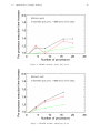
Performance tests on Hitachi SR8000 .
UKAFF: machine: grand; small model
UKAFF: machine: grand; large model
UKAFF: machine: ukaff; large model .
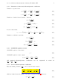
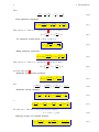
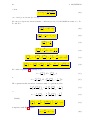
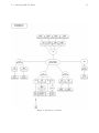
Program scheme . . . . . . . . . . . .
.
.
.
.
.
.
.
.
.
.
.
.
.
.
.
.
.
.
.
.
.
.
.
.
.
.
.
.
.
.
.
.
.
.
.
.
.
.
.
.
.
.
.
.
.
.
.
.
.
.
.
.
.
.
.
.
.
.
.
.
.
.
.
.
.
.
.
.
.
.
.
.
.
.
.
.
.
.
.
.
.
.
.
.
.
.
.
.
.
.
.
.
.
.
.
.
.
.
.
.
.
.
.
.
.
.
.
.
.
.
.
.
.
.
.
.
.
.
.
.
.
.
.
.
.
.
.
.
.
.
.
.
.
.
.
.
.
.
.
.
.
.
.
.
.
.
.
.
.
.
17
39
44
45
45
102
.
.
.
.
.
.
.
.
.
.
.
.
.
.
.
.
.
.
.
.
.
.
.
.
.
.
.
.
.
.
.
.
.
.
.
.
.
.
.
.
.
.
.
.
.
.
.
.
.
.
.
.
.
.
.
.
.
.
.
.
.
.
.
.
.
.
.
.
.
.
.
.
.
.
.
.
.
.
.
.
.
.
.
.
.
.
.
.
.
.
.
.
.
.
.
.
.
.
.
.
.
.
.
.
.
.
.
.
.
.
.
.
.
.
.
.
.
.
.
.
.
.
.
.
.
.
.
.
.
.
.
.
.
.
.
.
.
.
.
.
.
.
.
.
.
.
.
.
.
.
.
.
.
.
.
.
.
.
.
.
.
.
.
.
.
.
.
.
.
.
.
.
.
.
.
.
.
.
.
.
.
.
.
.
.
.
.
.
.
.
.
.
.
.
.
.
.
.
.
.
.
.
.
.
.
.
.
.
.
.
.
.
.
.
.
.
.
.
.
.
.
.
.
.
.
.
.
.
.
.
.
.
.
.
.
.
.
.
.
.
.
.
.
.
.
.
.
.
.
.
.
.
.
.
.
.
.
.
.
.
.
.
.
.
.
.
.
.
.
.
.
.
.
.
.
.
.
.
.
.
.
.
.
.
.
.
.
.
.
.
.
.
.
.
.
.
.
.
.
.
.
.
.
.
.
.
.
.
.
.
.
.
.
.
.
.
.
.
.
.
.
.
.
.
.
18
18
21
22
23
49
49
50
53
53
54
63
82
List of Tables
1
2
3
4
5
6
7
8
9
10
11
12
13
List of source directories . . . . .
List of old source directories . . .
List of all high-level modules . .
List of all low-level modules . . .
List of all old modules . . . . . .
UIO conversion types . . . . . . .
UIO entry types . . . . . . . . .
UIO header keywords . . . . . .
UIO Fortran90 files . . . . . . . .
Contents of uio base module.f90
Contents of uio mac module . . .
CO5BOLD control and data files
Radiation transport parameters .
.
.
.
.
.
.
.
.
.
.
.
.
.
.
.
.
.
.
.
.
.
.
.
.
.
.
.
.
.
.
.
.
.
.
.
.
.
.
.
5
1
Introduction
CO5BOLD – nickname COBOLD – is the short form of “COnservative COde for the COmputation of COmpressible COnvection in a BOx of L Dimensions with l=2,3”.
It is used to model solar and stellar surface convection. For solar-type stars only a small
fraction of the stellar surface layers are included in the computational domain. In the case of red
supergiants the computational box contains the entire star.
CO5BOLD solves the coupled non-linear equations of compressible hydrodynamics in an external gravity field together with non-local frequency-dependent radiation transport. Operator
splitting is applied to solve the equations of hydrodynamics (including gravity), the radiative
energy transfer (with a long-characteristics or a short-characteristics ray scheme), and possibly
additional 3D (turbulent) diffusion in individual sub steps. The 3D hydrodynamics step is further simplified with directional splitting. The 1D sub steps are performed with a Roe solver,
accounting for an external gravity field and an arbitrary equation of state from a table.
The radiation transport is computed with either one of three modules:
• MSrad module: It uses long characteristics. The lateral boundaries have to be periodic. Top
and bottom can be closed or open (“solar module”).
• LHDrad module: It uses long characteristics and is restricted to an equidistant grid and
open boundaries at all surfaces (old “supergiant module”).
• SHORTrad module: It uses short characteristics and is restricted to an equidistant grid and
open boundaries at all surfaces (new “supergiant module”).
There are preliminary versions of modules for the formation and advection of dust and the
transport of magnetic fields available.
CO5BOLD is written in Fortran90. The parallelization is done with OpenMP directives.
To get a brief overview you might want to look into the “Quickstart Sections” “How to Compile
CO5BOLD” (Sect. 3.1), “Introduction to UIO” (Sect. 4.1), “How to Make a Proper Parameter
File” (Sect. 5.3.1), “How to Run CO5BOLD” (Sect. 6.1).
6
2
2
EQUATIONS
Equations
2.1
Basic Equations
So far, this section demonstrates only how nicely LATEX can display formulae. . .
The 3D hydrodynamics equations, including source terms due to gravity, are the mass conservation equation
∂ρ ∂ ρ v1 ∂ ρ v2 ∂ ρ v2
+
+
+
=0 ,
(1)
∂t
∂x1
∂x2
∂x3
the momentum equation
ρv1
ρv1 v1 + P
ρv1 v2
ρv1 v3
ρ g1
∂
∂
∂
∂
ρv2 +
ρv2 v1
+
ρv2 v2 + P +
ρv2 v3
= ρ g2 (2)
∂t
∂x1
∂x2
∂x3
ρv3
ρv3 v1
ρv3 v2
ρv3 v3 + P
ρ g3
and the energy equation
∂ρeik ∂ (ρeik + P ) v1 ∂ (ρeik + P ) v2 ∂ (ρeik + P ) v3
+
+
+
= ρ (g1 v1 + g2 v2 + g3 v3). (3)
∂t
∂x1
∂x2
∂x3
In addition, there are equations for the 3D tensor viscosity and the non-local radiation transport.
2.2
2.2.1
A collection of thermodynamic relations (M. Steffen, AIP)
Basic thermodynamic equations
Differential relations:
p
dρ
ρ2
(4)
1
dh = T ds + dp
ρ
(5)
de = T ds +
where e is the internal energy .
where the specific enthalpy , h, is defined as
h = e + p/ρ
(6)
This implies:
∂e
∂s
∂e
∂ρ
=T
(7)
p
ρ2
(8)
=T
(9)
1
ρ
(10)
ρ
=
s
∂h
∂s
∂h
∂p
p
=
s
2.2
A collection of thermodynamic relations (M. Steffen, AIP)
2.2.2
7
Definition of often-used thermodynamic coefficients
Definition of specific heats:
cp ≡
cv ≡
∂h
∂T
∂e
∂T
=T
p
=T
ρ
∂s
∂T
∂s
∂T
=
p
=
ρ
∂s
∂ ln T
∂s
∂ ln T
(11)
p
(12)
ρ
Definitions of further thermodynamic coefficients:
χT ≡
∂ ln p
∂ ln ρ
∂ ln ρ
∂ ln T
χρ ≡
δ≡−
∂ ln p
∂ ln T
(13)
ρ
≡ (Kp)−1
(14)
T
≡ αT =
p
χT
χρ
(15)
It can be shown that
p 2
p
p 2
δ χρ =
δ χT =
χ /χρ
ρT
ρT
ρT T
cp − cv = α2 T /(Kρ) =
(16)
Definition of adiabatic exponents:
Γ1 ≡
Γ3 ≡
∇ad ≡
2.2.3
∂ ln p
∂ ln ρ
∂ ln T
∂ ln ρ
∂ ln T
∂ ln p
(17)
s
+1
(18)
Γ2 − 1
Γ2
(19)
s
≡
s
CO5BOLD equation of state
CO5BOLD equation of state input:
ρ; e
(20)
CO5BOLD equation of state output:
P; T;
All
required
thermodynamic
∂p
∂p
,
, ∂T
:
∂e
∂ρ
∂e
ρ
2.2.4
e
∂p
∂e
;
ρ
∂p
∂ρ
;
e
coefficients
∂T
∂e
can
(21)
ρ
be
expressed
in
terms
of
ρ
Derived thermodynamic coefficients
First, the missing derivative
∂T
∂ρ
e
∂T
∂ρ
can be found from the relation:
=
e
T
ρ2
∂p
∂e
−
ρ
p
ρ2
∂T
∂e
(22)
ρ
which is obtained from the equality of the mixed derivatives in Eq.4, written as:
ds =
1
p
de −
dρ
T
T ρ2
(23)
8
2
EQUATIONS
Then
∂2s
∂
=
∂e∂ρ
∂ρ
1
T
∂
p
− 2
∂e
Tρ
=
e
(24)
ρ
First adiabatic exponent:
Γ1 ≡
∂ ln p
∂ ln ρ
ρ
=
p
s
∂p
∂ρ
1
+
ρ
e
∂p
∂e
(25)
ρ
This relation is obtained by combining Eq.4 with the identity
∂p
∂ρ
dp =
∂p
∂e
dρ +
e
de
(26)
ρ
The adiabatic sound speed is then obtained as
s
cs ≡
∂p
∂ρ
p
ρ
r
=
Γ1
s
(27)
Third adiabatic exponent:
Γ3 ≡ 1 +
∂ ln T
∂ ln ρ
1
=1+
ρ
s
∂p
∂e
(28)
ρ
This relation is obtained by combining Eq.4 with the identity
dT =
∂T
∂ρ
dρ +
e
∂T
∂e
de
(29)
ρ
and then using Eq.22.
Adiabatic temperature gradient:
∇ad ≡
since
∂ ln T
∂ ln p
∂ ln T
∂ ln p
∂ ln T
∂ ln ρ
p
ρ
∂ρ
=e
∂p
=
s
=
s
·
s
Γ3 − 1
Γ1
∂ ln ρ
∂ ln p
(30)
=
s
Γ3 − 1
.
Γ1
(31)
Adiabatic energy changes:
ρ
∂e
∂p
=
s
∂ρ
∂p
=
s
∂ ln ρ
∂ ln p
=
s
1
Γ1
(32)
or
∂ρe
∂p
s
∂e
+ρ
∂p
s
1
ρe
=
1+
Γ1
p
s
(33)
We define the coefficients c0v and c0p through the relation
ds = c0v d ln p − c0p d ln ρ
(34)
Entropy change at constant density:
c0v
=
∂s
∂ ln p
ρ
p
=
ρT
∂ ln ρ
∂ ln T
=
s
p
1
ρT Γ3 − 1
(35)
2.2
A collection of thermodynamic relations (M. Steffen, AIP)
9
This relation is obtained from the equality of the mixed derivatives in Eq.4 together with Eq.28.
Entropy change at constant pressure:
c0p
∂s
=−
∂ ln ρ
p
p
=
ρT
∂ ln p
∂ ln T
p Γ1
ρT Γ3 − 1
=
s
(36)
This relation is obtained from the equality of the mixed derivatives in Eq.5 together with Eq.30.
Specific heat at constant density:
cv = c0v χT =
∂s
∂ ln T
=
ρ
∂e
∂T
= 1/
ρ
∂T
∂e
(37)
ρ
To derive the specific heat at constant pressure, we start from the relation
d ln T =
∂ ln T
∂ ln ρ
d ln ρ +
s
∂ ln T
∂s
ds
(38)
ρ
from which we get
∂s
∂ ln ρ
=−
T
∂ ln T
∂ ln ρ
/
s
∂ ln T
∂s
(39)
ρ
Using Eqs. 28 and 37, we obtain
Now
ds =
or
ds =
∂s
∂ ln p
∂s
∂ ln ρ
∂s
∂ ln p
d ln p +
ρ
= −cv (Γ3 − 1)
(40)
T
d ln p +
ρ
∂s
∂ ln ρ
p
∂s
∂ ln ρ
∂ ln ρ
∂ ln T
d ln ρ
(41)
p
d ln T +
s
∂ ln ρ
∂s
ds
(42)
T
hence
(
ds 1 −
∂s
∂ ln ρ
p
∂ ln ρ
∂s
)
=
T
∂s
∂ ln p
d ln p +
ρ
∂s
∂ ln ρ
p
∂ ln ρ
∂ ln T
d ln T
(43)
s
and finally
∂ ln T
∂s
(
=
1−
p
∂s
∂ ln ρ
p
∂ ln ρ
∂s
) (
/
T
∂s
∂ ln ρ
p
∂ ln ρ
∂ ln T
)
(44)
s
or
∂ ln T
∂s
=
p
∂ ln T
∂ ln ρ
(
s
∂ ln ρ
∂s
−
p
∂ ln ρ
∂s
)
(45)
T
Using Eqs. 11, 28, 36, 40, we finally obtain the relation for the specific heat at constant
pressure:
1
1
ρT (Γ3 − 1)2
1
=
−
=
−T
cp
cv
p
Γ1
cv
Γ3 − 1
cs
2
(46)
Alternatively, cp can be obtained from Eq.16
cp = cv +
p
δ χT
ρT
(47)
10
2
EQUATIONS
or from
Γ1
p
δ
ρT Γ3 − 1
cp = δ c0p =
(48)
once δ and χT are known (see below).
We can now express the thermodynamic coefficients provided by CO5BOLD in terms of cv , Γ1 ,
Γ3 , and ∇ad :
∂p
∂ρ
∂p
∂e
=
e
∂e
∂ρ
∂e
∂ρ
∂p
=−
∂ρ
=−
T
p
∂T
∂ρ
∂T
∂ρ
=
e
/
e
∂p
/
∂e
e
(49)
p
(1 − Γ3 + Γ1 )
ρ
(50)
∂T
∂e
= ρ (Γ3 − 1)
ρ
1
cv
(51)
T
p 1
(Γ3 − 1) − 2
ρ
ρ cv
(52)
∂T
∂e
ρ
=
ρ
p
ρ2
=
ρ
p
= 2
ρ
ρT
cv (Γ3 − 1)
p
1−
Γ1
1−
Γ3 − 1
p ∇ad − 1
ρ2 ∇ad
=
(53)
(54)
We consider again Eq.23, replacing de by
de =
so
1
ds =
T
∂e
∂T
∂e
∂T
dT +
ρ
dT +
ρ
1
T
∂e
∂ρ
∂e
∂ρ
dρ
(55)
T
p
−
T ρ2
T
dρ
(56)
The requirement that the mixed derivatives must be equal then yields
∂
∂ρ
1
T
∂e
∂T
!
ρ
T
∂e
∂ρ
∂
=
∂T
1
− 2
ρ
(
or
1
0=− 2
T
T
1
T
1
T
∂e
∂ρ
∂p
∂T
T
p
−
T ρ2
p
− 2
T
ρ
(57)
ρ
)
(58)
Finally,
∂e
∂ρ
T
p
= 2
ρ
(
1−
∂ ln p
∂ ln T
)
=
ρ
p
(1 − χT )
ρ2
(59)
Comparison with Eq.53 implies
χT =
ρT
cv (Γ3 − 1)
p
(60)
2.2
A collection of thermodynamic relations (M. Steffen, AIP)
11
Similarly, replacing de by
de =
∂e
∂p
dp +
ρ
∂e
∂ρ
dρ
(61)
p
in Eq.23, we get
1
ds =
T
∂e
∂p
(
dp +
ρ
1
T
∂e
∂ρ
p
−
T ρ2
p
)
dρ
(62)
and the requirement that the mixed derivatives must be equal then yields
∂
∂ρ
1
T
∂e
∂p
∂e
∂p
!
ρ
p
∂
=
∂p
or
∂T
∂ρ
∂ ln T
∂ ln ρ
ρ
=
p
∂T
∂p
1
T
(
ρ
or
∂e
∂p
Since
ρ
∂ ln T
∂ ln ρ
=
p
∂ ln T
∂ ln p
∂ ln T
/
∂ ln p
p
∂e
∂ρ
∂e
∂ρ
( ρ
p
ρ
p
− 2
ρ
p
∂e
∂ρ
∂ ln p
=−
∂ ln ρ
ρ
p
−
T ρ2
p
!
(63)
ρ
)
+
1
−
ρ
p
T
ρ2
)
1
+ .
ρ
(64)
(65)
= −χρ
(66)
T
we finally obtain, using Eqs.13, 49 and 54,
χρ = Γ1 − χT (Γ3 − 1)
(67)
δ = χT / {Γ1 − χT (Γ3 − 1)}
(68)
and
The isothermal sound speed is then obtained as
s
cT ≡
2.2.5
∂p
∂ρ
p
χρ =
ρ
r
=
T
s
p
Γ3 − 1
Γ1
1 − χT
ρ
Γ1
q
= cs (1 − χT ∇ad )
(69)
Ideal gas with constant specific heats (polytropic gas)
In this case, we obtain much simpler relations:
e = cv T =
p 1
ργ−1
(70)
h = cp T =
p γ
ργ−1
(71)
s = cv {ln p − γ ln ρ} + const.
cp
γ≡
= Γ1 = Γ2 = Γ3 = const.
cv
p
cp − cv =
≡R
ρT
1
= c0v
γ−1
γ
cp = R
= c0p
γ−1
cv = R
(72)
(73)
(74)
(75)
(76)
12
2
χT = χρ = δ = 1
s
cs ≡
∂p
∂ρ
s
cT ≡
∂p
∂ρ
r
=
γ
s
r
=
T
EQUATIONS
(77)
p
ρ
(78)
p
ρ
(79)
13
3
Program Files, Installation, Compilation
In this section all the files and modules CO5BOLD contains are listed. The installation procedure
is outlined and compiler switches necessary to compile CO5BOLD and to optimize its performance
are described.
3.1
Quickstart: How to Compile CO5BOLD
If you are going to install CO5BOLD on a machine with a “known” (to setup script and makefile)
operating system and compiler (see Sections 3.6 and 3.8) then the procedure should be fairly
easy. The general compilation procedure is now:
If a directory for the current machine exists (in the tar ball) and the configure script is there:
tar -zxvf for.tar.gz
cd for/hd/rhd/YOUR_MACHINE
./configure
make
If the directory for the current machine has to be created:
tar -zxvf for.tar.gz
cd for/hd/rhd
mkdir YOUR_MACHINE
cd YOUR_MACHINE
ln -s ../conf/configure .
./configure
make
The compilation process is explained in more detail in Sect. 3.2. The configure script is
described in its header and in Sect. 3.6. The directory structure is shown in Tab. 1. All Fortran
files are listed in Tables 3 and 4.
3.2
Compilation Procedure for CO5BOLD
The installation procedure has changed significantly since the last release: now, there is a configure
script (see Sect. 3.6) that creates the complete (temporary) makefile which can be used to compile
CO5BOLD and produce the executable rhd.exe.
Installation procedure:
1. Choose/create a proper base directory. (This will usually be $HOME. Then the master
directory will typically be $HOME/for – this is the default created by the tar file. Some
prefer to rename it to $HOME/HYDRO.)
2. Put all source files and the configure script there. This will be done typically by expanding
the gzipped tar file for.tar.gz e.g. with
tar -zxvf for.tar.gz
(or by copying all files from an existing installation). On a restricted UNIX you might be
forced to use
gunzip for.tar.gz
tar -xvf for.tar
instead. Unpacking the tar file creates a sub directory for in the local directory (and
possible overwrites existing files!). You get sub sub directories as described in Sect. 3.3 and
files as listed in Tables 3 and 4. See the Readme file ’for/README’.
14
3
PROGRAM FILES, INSTALLATION, COMPILATION
3. Change with
cd for/hd/rhd
into the main directory.
4. Look at the existing sub directories, e.g. with
ls -og | grep "^d"
to see if you find one that fits your machine. The directory
for/hd/rhd/conf
should not be used. It contains only the configure script. But any other directory will do.
If you don’t like any of the existing directories, create your own e.g. with
mkdir YOUR_MACHINE
Change into this directory with
cd YOUR_MACHINE
5. Check if there is a configure script or a link to it with
ls -og configure
which should give something like
lrwxrwxrwx
1
17 2002-12-04 17:39 configure -> ../conf/configure
If it is not there, create the link with
ln -s ../conf/configure .
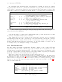
6. Start the configure script to create the (first version of the) Makefile
./configure
This gives you a screen output like
Configuration script for CO5BOLD Makefile
=========================================
No
No
No
No
No
No
No
No
parallelization requested, assume default:
debugging requested, assume default:
LHDrad
module requested, assume default:
MSrad
module requested, assume default:
SHORTrad module requested, assume default:
dust
module requested, assume default:
MHD
module requested, assume default:
explicit machine requested, assume default:
List of control environment variables:
F90_COMPILER =
F90_PARALLEL=scalar
F90_DEBUG=0
F90_LHDRAD=0
F90_MSRAD=0
F90_SHORTRAD=1
F90_DUST=0
F90_MHD=0
F90_MACHINE=local
3.2
Compilation Procedure for CO5BOLD
F90_PREFLAGS =
F90_POSTFLAGS=
F90_PARALLEL =
F90_DEBUG
=
F90_LHDRAD
=
F90_MSRAD
=
F90_SHORTRAD =
F90_DUST
=
F90_MHD
=
F90_MACHINE =
-> MACHINE =
F90_BASEPATH =
15
scalar
0
0
0
1
0
0
local
i686
/home/bf/for
Linux system with i686 architecture
PGI compiler
version=3.3-2
pgf90 -byteswapio -fast -Mvect=sse -Mcache_align -Minfo=inline
Write compiler name and flags into file compiler_flags.info
Makefile already exists. It is appended to Makefile_old.
New Makefile written..........................................
A new ’Makefile’ is produced. An existing one is appended to ’Makefile_old’. Additionally, the file ’compiler_flags.info’ is written which contains the compiler call in Fortran
format.
7. Check the output of the configure script and the header of the new Makefile. You get
an overview over the relevant environment variables that control the configure script (see
Sect. 3.6) with
env | grep F90_
Obs: at the beginning there might be none.
8. Look into the header (and if necessary the rest) of the configure script or into Sect. 3.6
to find out how to change the environment variables to control the script properly. For
instance, if you want to enable debugging options, type:
export F90_DEBUG=1
Restart the configure script after every change in the control variables! With e.g.
export F90_MACHINE=dummy
export F90_PREFLAGS="-Oprettyfast +Qsomethingelse"
./configure
it is possible to specify all machine-dependent settings yourself (see Sect. 3.6 and Sect. 3.6).
This is useful when dealing with a compiler hitherto unknown to the configure script.
9. Start the compilation with
make
to produce the executable rhd.exe.
16
3
PROGRAM FILES, INSTALLATION, COMPILATION
A simple sample installation may look like the following (the sub directory ’for’ is put into
the home directory).
# --- Choose base directory --cd $HOME
# --- Put the tar file there --# ...
# --- Expand the tar file --tar -zxvf for.tar.gz
# --- Go into (default) master directory --cd for/hd/rhd/YOUR_MACHINE
# --- Activate OpenMP und MSrad radiation transport --export F90_PARALLEL=openmp
export F90_MSRAD=1
# --- Start the configure script --./configure
# --- Compile --make
echo ’Voila!’
If you want to compile in a directory in a completely different place (not in a sub directory of
for as described above), you have to set the environment variable F90_BASEPATH (see Sect. 3.6)
to make the paths to the source files known to the configure script. That might look like
mkdir SOME_WEIRD_PLACE
cd SOME_WEIRD_PLACE
export F90_BASEPATH=$HOME/for
ln -s $F90_BASEPATH/hd/rhd/conf/configure .
./configure
The variable F90_BASEPATH also has to be set explicitely if the main directory for should
have another name. Renaming the sub-directories with the source files is not a good idea – it
requires modifications of the configure script itself.
3.3
Directory Structure
The files necessary to compile CO5BOLD are distributed over a few directories. A typical setup
would be to put everything into the main directory for. Then the source files would be located
as in Tab. 1.
The executables (and makefiles, object files, module information files) are usually located in
subdirectories of the source code directories. These subdirectories typically have the name of the
machine, architecture, or operating system the executable is compiled for.
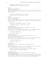
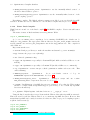
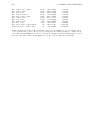
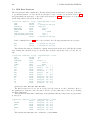
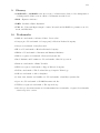
The former directory organization can be found in Tab. 2 and Fig. 1.
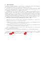
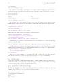
3.4
Old Setup File for Paths
For the previous version of CO5BOLD all paths were stored in environment variables and could
be set with the scripts
3.4
Old Setup File for Paths
17
Figure 1: Old directory scheme
18
3
Paths
${HOME}/for/con/f90/
${HOME}/for/dust/f90/
${HOME}/for/eos/f90/
${HOME}/for/hd/mhd/
${HOME}/for/hd/rhd/
${HOME}/for/hd/rhdb/
${HOME}/for/mat/str/
${HOME}/for/opa/opta/
${HOME}/for/rad/hdrad/
${HOME}/for/uio/f90/
${HOME}/for/time/f90/
Abb.
CON
DUST
EOS
MHD
RHD
RHDB
STR
OPTA
RAD
UIO
TIME
PROGRAM FILES, INSTALLATION, COMPILATION
Description
constants and units
source terms due to dust or molecules
equation of state
MHD routines
main rhd routines (hydro, Bernd’s radiation transport)
basic rhd routines
string handling
opacities
Matthias’ radiation transport
I/O routines
timing routines
Table 1: List of source directories with path and file name, abbreviation, and a short description.
Paths
${HOME}/for/mat/str/
${HOME}/for/uio/f90/
${HOME}/for/eos/f90/
${HOME}/for/rad/hdrad/
${HOME}/for/hd/rhd/
Abb.
STR
UIO
EOS
RAD
RHD
Description
string handling
I/O routines
equation of state
opacities, Matthias’ radiation transport
main rhd routines
Table 2: For historical reasons: list of old source directories with path and file name, abbreviation,
and a short description.
setarcdeppaths.sh
or
setarcdeppaths.csh .
These variables are now ignored by the configure script that produces the Makefile to generate
the CO5BOLD executable rhd.exe.
However, they are still used e.g. by the makefile that produces the executables that are called
by the UIO scripts. The environment variables for the UIO routines can be e.g.
UIOSRCPATH=/home/user/for/uio/f90
UIOEXEPATH=/home/user/for/uio/f90/sun .
A script to set all necessary variables and paths can be (here for the Bourne shell)
#!/bin/sh
#
# --- Disk where all Fortran programs are located --FORTRANDISK=$HOME/for ; export FORTRANDISK
#
if [ ‘uname -s‘ = "craSH" ]; then
# --- Kiel: craSHi --#
UIOMAC=uio_mac_crayxmp_module ; export UIOMAC
RHDMAC=rhd_mac_cray_module ; export RHDMAC
elif [ ‘uname -s‘ = "craSH" ]; then
# --- Kiel: craSH --#
UIOMAC=uio_mac_crayts_module ; export UIOMAC
RHDMAC=rhd_mac_cray_module ; export RHDMAC
elif [ ‘uname -m‘ = "SR8000" ]; then
3.4
Old Setup File for Paths
# --- Potsdam: Hitachi --#
UIOMAC=uio_mac_hitachi_module ; export UIOMAC
RHDMAC=rhd_mac_hitachi_module ; export RHDMAC
else
# --- Default: Suns MAC files --#
UIOMAC=uio_mac_sun_module; export UIOMAC
RHDMAC=rhd_mac_sun_module; export RHDMAC
fi
#
# --- Architecture dependent sub directory names for object file and executables --if [ ‘uname -s‘ = "craSH" ]; then
MAC=crash
elif [ ‘uname -s‘ = "craSHi" ]; then
MAC=crashi
elif [ ‘uname -s‘ = "SunOS" ]; then
MAC=sun
elif [ ‘uname -s‘ = "HP-UX" ]; then
if [ ‘uname -m‘ = "ia64" ]; then
MAC=hpia64
else
MAC=hp
fi
elif [ ‘uname -s‘ = "Linux" ]; then
MAC=linux
elif [ ‘uname -n‘ = "vx1" ]; then
MAC=vx1
else
MAC=sgi
fi
#
# --- Individual libraries --# --- Timing --TIMEPATH=$FORTRANDISK/time/f90 ; export TIMEPATH
TIMESRCPATH=$TIMEPATH ; export TIMESRCPATH
#
# --- Constants & units --CONPATH=$FORTRANDISK/con/f90 ; export CONPATH
CONSRCPATH=$CONPATH ; export CONSRCPATH
#
# --- uio --UIOPATH=$FORTRANDISK/uio ; export UIOPATH
UIOSRCPATH=$UIOPATH/f90 ; export UIOSRCPATH
#
# --- String handling --STRPATH=$FORTRANDISK/mat/str ; export STRPATH
STRSRCPATH=$STRPATH ; export STRSRCPATH
#
# --- Math --MATPATH=$FORTRANDISK/mat ; export MATPATH
MATSRCPATH=$MATPATH/f90 ; export MATSRCPATH
#
# --- gas --GASPATH=$FORTRANDISK/eos/gas ; export GASPATH
GASSRCPATH=$GASPATH ; export GASSRCPATH
#
# --- EOS --EOSPATH=$FORTRANDISK/eos ; export EOSPATH
EOSSRCPATH=$EOSPATH/f90 ; export EOSSRCPATH
#
19
20
3
PROGRAM FILES, INSTALLATION, COMPILATION
# --- Opacity --OPTAPATH=$FORTRANDISK/opa/opta ; export OPTAPATH
OPTASRCPATH=$OPTAPATH ; export OPTASRCPATH
#
# --- hydrostatic --HSTPATH=$FORTRANDISK/hd/qf15 ; export HSTPATH
HSTSRCPATH=$HSTPATH ; export HSTSRCPATH
#
# --- rad --RADPATH=$FORTRANDISK/rad/hdrad ; export RADPATH
RADSRCPATH=$RADPATH ; export RADSRCPATH
#
# --- RHD --RHDPATH=$FORTRANDISK/hd/rhd ; export RHDPATH
RHDSRCPATH=$RHDPATH ; export RHDSRCPATH
#
# --- RHDB --RHDBPATH=$FORTRANDISK/hd/rhdb ; export RHDBPATH
RHDBSRCPATH=$RHDBPATH ; export RHDBSRCPATH
#
# --- HDW --HDWPATH=$FORTRANDISK/hd/hdw ; export HDWPATH
HDWSRCPATH=$HDWPATH ; export HDWSRCPATH
#
# --- DUST --DUSTPATH=$FORTRANDISK/hd/dust ; export DUSTPATH
DUSTSRCPATH=$DUSTPATH ; export DUSTSRCPATH
#
# --- MHD --MHDPATH=$FORTRANDISK/hd/mhd ; export MHDPATH
MHDSRCPATH=$MHDPATH ; export MHDSRCPATH
#
# --- mean --MEANPATH=$FORTRANDISK/hd/mean ; export MEANPATH
MEANSRCPATH=$MEANPATH ; export MEANSRCPATH
#
# --- Architecture dependent directories for object file and executables --TIMEEXEPATH=$TIMEPATH/$MAC
; export TIMEEXEPATH
CONEXEPATH=$CONPATH/$MAC
; export CONEXEPATH
UIOEXEPATH=$UIOSRCPATH/$MAC ; export UIOEXEPATH
STREXEPATH=$STRPATH/$MAC
; export STREXEPATH
MATEXEPATH=$MATSRCPATH/$MAC ; export MATEXEPATH
GASEXEPATH=$GASPATH/$MAC
; export GASEXEPATH
EOSEXEPATH=$EOSSRCPATH/$MAC ; export EOSEXEPATH
OPTAEXEPATH=$OPTAPATH/$MAC
; export OPTAEXEPATH
HSTEXEPATH=$HSTPATH/$MAC
; export HSTEXEPATH
RADEXEPATH=$RADPATH/$MAC
; export RADEXEPATH
RHDEXEPATH=$RHDPATH/$MAC
; export RHDEXEPATH
RHDBEXEPATH=$RHDBPATH/$MAC
; export RHDBEXEPATH
HDWEXEPATH=$HDWPATH/$MAC
; export HDWEXEPATH
DUSTEXEPATH=$DUSTPATH/$MAC
; export DUSTEXEPATH
MHDEXEPATH=$MHDPATH/$MAC
; export MHDEXEPATH
MEANEXEPATH=$MEANPATH/$MAC
; export MEANEXEPATH
This script can be executed with
. $HOME/bin/setarcdeppaths.sh
This line can be put e.g. into the .bashrc file.
Some lines can be edited to account for individual choices and the target machine. With
FORTRANDISK=$HOME/for ; export FORTRANDISK
3.5
Fortran Files
21
the master directory is specified. With
UIOMAC=uio_mac_sun_module; export UIOMAC
RHDMAC=rhd_mac_sun_module; export RHDMAC
you set some machine dependent modules. The sun modules work for most machines (e.g. for
Linux Intel/AMD machines). With
MAC=linux
you specify the name of the subdirectories with the makefiles. The other lines only have to be
edited if you want to organize the directories in a completely different way. In this case you have
to adapt the configure script, too.
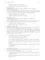
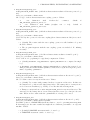
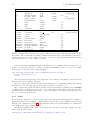
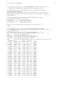
3.5
Fortran Files
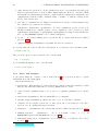
Tables 3 and 4 show a list of all source files necessary to compile the complete version of
CO5BOLD. Table 5 shows the former list.
File and path
hd/rhd/rhd.F90
hd/rhd/rhd_hyd_module.F90
hd/rhd/rhd_lhdrad_module.F90
Abb.
RHD
RHD
RHD
hd/rhd/rhd_shortrad_module.F90
RHD
hd/rhd/rhd_shortrad_dtauop01.f90
hd/rhd/rhd_shortrad_dtauop02.f90
hd/rhd/rhd_shortrad_operator00.f90
...
hd/rhd/rhd_shortrad_operator08.f90
hd/rhd/rhd_vis_module.F90
rad/hdrad/rhd_rad_module.f90
rad/hdrad/MSrad3D.F90
RHD
RHD
RHD
hd/dust/rhd_dust_module.F90
hd/dust/dust_k3mon_module.f
dust_momentc2_module.f
C2.INC
C2H.INC
C2H2.INC
CHPAR_CT.INC
DINDEX.INC
DKSPLINT.INC
H2.INC
hd/mhd/rhd_mhd_module.F90
eos/f90/gasinter_routines.f90
opa/opta/cubit_module.f
opa/opta/opta_par_module.f90
opa/opta/opta_routines.f
DUST
DUST
DUST
DUST
DUST
DUST
DUST
DUST
DUST
DUST
MHD
EOS
OPTA
OPTA
OPTA
RHD
RHD
RAD
RAD
Description
main program
hydrodynamics routines
radiative transfer routines,
long characteristics, supergiant case
radiative transfer routines,
short characteristics, supergiant case
short characteristics tau-coupling
short characteristics tau-coupling
short characteristics operator
short characteristics operator
tensor viscosity routines
interface for Matthias’ radiation routine
Matthias’ radiation transport routines,
long characteristics, periodic sides
dust/molecule formation
1 or 2 component dust model
4 moment dust model
dust include file: C2 molecule
dust include file: C2 H molecule
dust include file: C2 H2 molecule
dust include file
dust include file
dust include file
dust include file: H2 molecule
magnetic fields (first version)
equation of state
cubic interpolation
parameters for opacity routines
opacity
Table 3: List of all high-level modules: the table shows the file name with part of its path, the
shortcut for the directory, and its description.
22
3
PROGRAM FILES, INSTALLATION, COMPILATION
File and path
hd/rhdb/rhd_action_module.f90
hd/rhdb/rhd_box_module.f90
hd/rhdb/rhd_dat_module.f90
hd/rhdb/rhd_gl_module.f90
hd/rhdb/rhd_io_module.f90
hd/rhdb/rhd_mac_cray_module.f90
hd/rhdb/rhd_mac_default_module.f90
hd/rhdb/rhd_mac_hitachi_module.f90
hd/rhdb/rhd_mac_sun_module.f90
hd/rhdb/rhd_mean_module.f90
hd/rhdb/rhd_prop_module.f90
hd/rhdb/rhd_sub_module.f90
con/f90/const_module.f90
mat/str/str_module.f90
time/f90/timing_module.f90
uio/f90/uio_base_module.f90
uio/f90/uio_bulk_module.f90
uio/f90/uio_filedef_module.f90
uio/f90/uio_mac_crayts_module.f90
uio/f90/uio_mac_crayxmp_module.f90
uio/f90/uio_mac_decalpha_module.f90
uio/f90/uio_mac_hitachi_module.f90
uio/f90/uio_mac_ieee_module.f90
uio/f90/uio_mac_intel_module.f90
uio/f90/uio_mac_module.f90
uio/f90/uio_mac_nec_module.f90
uio/f90/uio_mac_sun_module.f90
Abb.
RHDB
RHDB
RHDB
RHDB
RHDB
RHDB
RHDB
RHDB
RHDB
RHDB
RHDB
RHDB
CON
STR
TIME
UIO
UIO
UIO
UIO
UIO
UIO
UIO
UIO
UIO
UIO
UIO
UIO
Description
routines for control parameter passing
box handling routines
handling of additional data (averages)
global parameters
input/output routines
machine dependent routines (CRAY)
machine dependent routines (default)
machine dependent routines (Hitachi)
mac-dependent routines (Sun, others)
averaging routines
box properties
additional routines
physical and mathematical constants
string handling
timing routines
I/O routines
I/O routines
I/O routines
I/O routines, machine dependent part
I/O routines, machine dependent part
I/O routines, machine dependent part
I/O routines, machine dependent part
I/O routines, machine dependent part
I/O routines, machine dependent part
I/O routines, m.-d., minimal version
I/O routines, machine dependent part
I/O, m.-d., works in most cases
Table 4: List of all low-level modules: the table shows the file name with part of its path, the
shortcut for the directory, and its description.
3.5
Fortran Files
23
File and path
mat/str/str_module.f90
uio/f90/uio_base_module.f90
uio/f90/uio_bulk_module.f90
uio/f90/uio_filedef_module.f90
uio/f90/uio_mac_sun_module.f90
eos/f90/gasinter_routines.f90
rad/hdrad/cubit_module.f
rad/hdrad/opta_par_module.f90
rad/hdrad/opta_routines.f
rad/hdrad/MSrad3D.F90
Abb.
STR
UIO
UIO
UIO
UIO
EOS
RAD
RAD
RAD
RAD
hd/rhd/timing_module.f90
hd/rhd/rhd_const_module.f90
hd/rhd/rhd_gl_module.f90
hd/rhd/rhd_action_module.f90
hd/rhd/rhd_box_module.f90
hd/rhd/rhd_dat_module.f90
hd/rhd/rhd_mean_module.f90
hd/rhd/rhd_io_module.f90
hd/rhd/rhd_mac_cray_module.f90
hd/rhd/rhd_mac_default_module.f90
hd/rhd/rhd_mac_sun_module.f90
hd/rhd/rhd_sub_module.f90
hd/rhd/rhd_hyd_module.F90
hd/rhd/rhd_vis_module.F90
hd/rhd/rhd_rad_module.f90
hd/rhd/rhd_lhdrad_module.F90
RHD
RHD
RHD
RHD
RHD
RHD
RHD
RHD
RHD
RHD
RHD
RHD
RHD
RHD
RHD
RHD
hd/rhd/rhd_shortrad_module.F90
RHD
hd/rhd/rhd.F90
RHD
Description
string handling
I/O routines
I/O routines
I/O routines
I/O routines, machine dependent part
equation of state
cubic interpolation
parameters for opacity routines
opacity
Matthias’ radiation transport routines,
long characteristics, periodic sides
timing routines
physical and mathematical constants
global parameters
routines for control parameter passing
box handling routines
handling of additional data (averages)
averaging routines
input/output routines
machine dependent routines (CRAY)
machine dependent routines (default)
machine dependent routines (Sun)
additional routines
hydrodynamics routines
tensor viscosity routines
interface for Matthias’ radiation routine
radiative transfer routines,
long characteristics, supergiant case
radiative transfer routines,
short characteristics, supergiant case
main program
Table 5: For historical reasons: list of all old modules: the table shows the file name with part of
its path, the shortcut for the directory, and its description.
24
3
3.6
PROGRAM FILES, INSTALLATION, COMPILATION
Configure Script
The configure script produces a Makefile.
It is controlled by environment variables (see below). It tries to use reasonable default values
if they are not set (properly). In the script the machine type is determined with ‘uname m‘. According to the control variables and the machine architecture the compiler name and its
compiler flags are composed. These are written into the header of a Makefile which is produced
in the end. An existing Makefile is appended to
Makefile_old.
Additionally the compilation command is written into the file
’compiler_flags.info’
in a form ready to be included in a Fortran program.
The environment variables that control the script are
• F90_COMPILER:
Fortran compiler:
◦ ’’: a machine dependent default is chosen individually for each architecture
◦ f90: general default
• F90_PREFLAGS:
Compiler flags to be put at the beginning of the list. Usually, the list of compiler flags
produced by the configure script should be pretty complete. But you might want to add
special switches like ’-Bstatic’ to enforce static linking of libraries.
◦ ’’: No extra flags
• F90_POSTFLAGS:
Compiler flags to be put at the end of the list. Usually, the list of compiler flags produced
by the configure script should be pretty complete. However, you might want to overwrite
some settings. This can be done by setting this variable to a none-empty value because
typically a compiler should interpret the flags from left to right.
◦ ’’: No extra flags
• F90_PARALLEL:
Parallelization scheme:
◦ scalar: no parallelization (default)
◦ openmp: OpenMP (appropriate for CO5BOLD)
◦ auto: auto-parallelization (not implemented for all machines)
• F90_DEBUG:
Debugging level:
◦ 0: No extra debugging information produced, full optimization is chosen (default)
◦ 1: standard debugging mode (typically switch ’-g’ instead of ’-fast’)
◦ 2: other debbuging (or array checking) modes possible if implemented for the requested
machine
• F90_LHDRAD:
LHDrad radiation transport:
◦ 0: do not activate (compile and link) this module (default)
◦ 1: activate this radiation transport module
3.7
Compiler Macros
25
• F90_MSRAD:
MSrad radiation transport:
◦ 0: do not activate (compile and link) this module (default)
◦ 1: activate this radiation transport module
• F90_SHORTRAD:
SHORTrad radiation transport:
◦ 0: do not activate (compile and link) this module (default)
◦ 1: activate this radiation transport module
• F90_DUST:
DUST module:
◦ 0: do not activate (compile and link) this module (default)
◦ 1: activate this source step module
If this variable is set to 1 the compiler is called with -Drhd_box_quc01=1, see Sect. 3.7.
• F90_MHD:
MHD module:
◦ 0: do not activate (compile and link) this module (default)
◦ 1: activate this magnetohydrodynamics module
• F90_MACHINE:
Explicit machine specification. This isusually not necessary, use ’local’ or ” instead.
◦ ’’: local machine
◦ sun4u: Sun
◦ . . . : See the header of the configure script for an up to date list
◦ local: local machine (default)
◦ dummy: Do not use any machine dpedendent flags but use module selections
◦ empty: Compiler flags are composed from F90_PREFLAGS and F90_POSTFLAGS only
• F90_BASEPATH:
Path for CO5BOLD base directory.
◦ ’’: The configure script tries to determine the base directory name automatically (default). This should work if the local directory is located somewhere below .../hd/rhd/
◦ otherwise: This string is used as base directory name (e.g. /home/user/for)
Some examples can be found in Sect. 3.2.
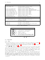
3.7
Compiler Macros
Some of the modules of the CO5BOLD code (with suffix “.F90”) employ compiler macros to
switch between code versions during compile time. Typically you define at least one of the three
switches rhd_r01, rhd_r02, or rhd_r03 to choose a radiation transport module. The others have
reasonable default values. To find the combination with the optimal performance, you should
look into Sect. 3.8
The macros are sorted into different categories:
Some activate a certain feature (like a radiation transport module or the dust module). They
have to be selected by the user (typically via environment variables and the configure script, see
Sect. 3.6) each time the code is compiled for a certain purpose.
26
3
PROGRAM FILES, INSTALLATION, COMPILATION
Other macros are meant to improve the performance by offering the choice between e.g.
different loop structures or case distinctions. These macros are set by the configure script to the
best knowledge of the author(s). Ideally, they should be checked and modified if necessary each
time CO5BOLD is compiled on a new machine. It should be save to modify these settings: the
results between runs with different settings should only differ slightly due to round-off errors.
Some macros select between different numerical approximations. A change here should be
visible in a (more or less drastic) change of the results of a simulation. Usually, the default values
should be accepted. Other settings typically only exist to allow the comparison with older versions
of CO5BOLD or because there are new developments going on which have not yet managed to
become the default.
A couple of macros only activate timing measurements and result in additional output. Some
of them are not thread-save und should only be activated for runs on one thread (as done by the
configure script). It is always save to switch any of them off (by removing or undefining them).
The macros in the category test mark parts of code under development. The default values
should only be changed with great care (typically by the author of that code segment). The
configure script does not touch these settings.
General:
• timing_c_factor:
in timing_module.F90, (“timing count factor”).
Category: account for property of machine.
To produce the timing statistics printed at the end of a simulation run the standard Fortran
routine SYSTEM_CLOCK is used. The macro timing_c_factor specifies by how much the
count rate of this routine is reduced when storing its count value. This does not prevent all
overflows but can make the output much more useful. Values:
◦ 1: (default) count rate of SYSTEM_CLOCK is used directly.
◦ otherwise: e.g. 1000, count rate of SYSTEM_CLOCK is reduced by this factor.
By a proper choice of this factor the timing measurements of individual routines can be
made meaningful: the reduction of the count rate prevents overflows due to the addition of
several measurements. An overflow during an individual measurement can not be prevented.
Therefore, the count rate for the entire program still tends to produce overflows.
• gasinter_l01:
in gasinter_routines.F90, (“gas interpolation l01”).
Category: performance enhancement.
This switch determines how temporary arrays are handled to improve performance Values:
◦ 0: (default) Temporary coefficient arrays are actually copied.
◦ 1: Temporary coefficient arrays just get a pointer link into the big arrays.
• rhd_box_grav01:
in rhd_box_module.F90, (“rhd box gravitation 01”).
Category: feature activation.
Switch to activate the array for the gravitational potential in the box structure. If the
switch is set to 1, a 3D array for the potential is created, copied, removed, ... There is
no module to compute the gravitational potential, yet. Therefore the entire thing has no
practical value, yet. Values:
◦ 0: (default) no handling of array.
◦ 1: array handling activated.
• rhd_box_quc01:
in rhd_box_module.F90 and rhd.F90, (“rhd box quantity centered 01”).
Category: feature activation.
3.7
Compiler Macros
27
Now, CO5BOLD is able to handle a number of additional quantities (e.g. density arrays)
in addition to the basic hydrodynamics quantities (ρ, ei, ...) if this compiler switch is
activated. These additional quantities can be e.g. densities of dust distribution moments or
densities of molecules. Values:
◦ 0: (default) no handling of additional quantities (density arrays).
◦ 1: handling of additional density arrays is activated.
To actually include dust formation in a simulation, it is necessary to
1. set the switch -Drhd_box_quc01=1 during compilation (this is done by the configure
script if the environment variable F90_DUST is set to 1, see the description of the
variable in Sect. 3.6),
2. put arrays specifying the initial conditions of the additional density into the start
model (as real quc001, real quc002, ...),
3. select a proper model describing dust (or molecule) formation in the parameter file
(with character dustscheme).
• rhd_box_bmag01:
in rhd_box_module.F90 and rhd.F90, (“rhd box b magnetic 01”).
Category: feature activation.
CO5BOLD can handle magnetic field arrays if this compiler switch is set. Values:
◦ : (default) no handling of magnetic field arrays.
◦ : handling of magnetic field arrays is activated.
To actually account for magnetic fiels in a simulation, it is necessary to
1. set the switch -Drhd_box_bmag01=1 during compilation (this is done by the configure
script if the environment variable F90_MHD is set to 1, see Sect. 3.6),
2. put arrays specifying the initial conditions of the boundary centered magnetic field
arrays into the start model (as real bb1, real bb2, real bb3),
3. select an hydrodynamics scheme that is able to handle magnetic fields in the parameter
file (with character hdscheme).
Hydrodynamics (Roe solver):
• rhd_roe1d_slope_l01:
in rhd_hyd_module.F90, (“rhd roe 1 dimension slope loop 01”).
Category: feature activation.
When this compiler switch is set, a new extra stabilization mechanism can be activated: If
one of the reconstruction methods VanLeer, Superbee, or PP (see Sect. 5.3.7) is activated,
the slope can be reduced (by averaging with the results from a MinMod reconstruction) by
setting c_slopered (see Sect. 5.3.7) to a positive non-zero value. This can improve the
stability without significantly reducing the effective numerical resolution. Switch values:
◦ 0: (default) no slope reduction.
◦ 1: slope reduction in case of expansion wave.
◦ 2: slope reduction in case of strong density contrast.
• IDF:
in rhd_hyd_module.F90, (“Integer Delta Flux”).
Category: performance enhancement.
Number of padding cells for flux-like variables. This number was introduced to check
whether the increase of the size of vectors for flux-like quantities (defined at cell boundaries)
can improve the performance (especially on a CRAY machine). The gain is marginal (if
present at all). The parameter is usually set to zero or left undefined. Values:
28
3
PROGRAM FILES, INSTALLATION, COMPILATION
◦ 0: (default) no padding cells
◦ 1,2,3,. . . : extra padding cells
• rhd_hyd_gravcorr_p01:
in rhd_hyd_module.F90, (“rhd hydrodynamics gravitation correction parameter 01”).
Category: selection of approximation.
This parameter controls the way the Roe solver handles the source terms due to gravity.
A different choice results in different simulation results and not just in slightly faster (or
slower) code. The problem is that the original Roe solver interpretes the pressure gradient in
a hydrostatic stratification a fluctuation due to shock waves. In case of strong stratification
this can lead to weird effects. With activated correction the Roe solver treats only the
deviations from a hydrostatic stratification as due to waves (or shocks). Several correction
formulas have been tried. The latest is the recommended default. Values:
◦ 0: No pressure correction terms in Roe solver.
◦ 1: Simple correction with rhomean, no new average pressure.
◦ 2: Simple correction with rhomean, new average pressure.
◦ 3: Correction with local rho, limited, new average pressure.
◦ 4: Correction with local rho, new (different formula) average pressure.
◦ 5: (default) Correction with local rho, new limit, new average pressure.
• rhd_hyd_entropyfix_p01:
in rhd_hyd_module.F90, (“rhd hydrodynamics entropy fix parameter 01”).
Category: performance enhancement.
The entropy fix can be done in one of two ways to get optimum performance (with essentially
the same results). Values:
◦ 0: (default) “if. . . then. . . else” construction
◦ 1: use a mask and the signum function
• rhd_hyd_upwind_p01:
in rhd_hyd_module.F90, (“rhd hydrodynamics upwind parameter 01”).
Category: performance enhancement.
The determination of the upwind direction can be done in one of two ways to get optimum
performance (with essentially the same results). Values:
◦ 0: (default) “if. . . then. . . else” construction
◦ 1: use a mask and the signum function
• rhd_hyd_roe1d_l01:
in rhd_hyd_module.F90, (“rhd hydrodynamics roe 1 dimension loop 01”).
Category: performance enhancement.
The computation of the Roe fluxes can be done by either of two sets of routines to find the
set which gives optimum performance (with essentially the same results). Values:
◦ 0: (default) lots of small routines acting on scalars, inlining needed, cache reuse is
optimized
◦ 1: routines acting on arrays, more temporary arrays necessary, vectorization is easier
• rhd_roe1d_flux_l01:
in rhd_hyd_module.F90, (“rhd roe 1 dimension flux loop 01”).
Category: test.
By setting this switch an alternative way of computing the upwind centered Roe states is
activated (only for ’constant’ reconstruction, for performance test purposes only: do not
activate!). Values:
3.7
Compiler Macros
29
◦ undefined: (default) Use standard method to compute the Roe states.
◦ defined: Use non-standard method to compute the Roe states.
• rhd_bound_t01:
in rhd_hyd_module.F90, (“rhd bound timing 01”).
Category: additional output.
Produce timing information for “inner boundary” routine (central potential) or lower and
upper boundary routines (constant gravitation). It can be used together with OpenMP.
Values:
◦ undefined: (default) no timing information.
◦ defined: call subroutines to measure elapsed time.
• rhd_roe1d_flux_t01:
in rhd_hyd_module.F90, (“rhd roe 1 dimension flux timing 01”).
Category: additional output.
Produce timing information for the routine which computes the Roe fluxes. It should not
be used in conjunction with OpenMP. Values:
◦ undefined: (default) no timing information
◦ defined: call subroutines to measure elapsed time
• rhd_roe1d_step_t01:
in rhd_hyd_module.F90, (“rhd roe 1 dimension step timing 01”).
Category: additional output.
Produce timing information for the routine which performs the Roe step. It should not be
used in conjunction with OpenMP. Values:
◦ undefined: (default) no timing information
◦ defined: call subroutines to measure elapsed time
Hydrodynamics (tensor viscosity):
• rhd_vis_density_p01:
in rhd_vis_module.F90, (“rhd viscosity density parameter 01”).
Category: selection of approximation.
Choose formula for density average at cell boundary in tensor viscosity routines. Values:
◦ 0: rhomean=min(rholeft,rhoright)
◦ 1: (default) rhomean=0.5 * (rholeft + rhoright)
• rhd_vis_t01:
in rhd_vis_module.F90, (“rhd viscosity timing 01”).
Category: additional output.
Produce timing information for 2D/3D tensor viscosity routines. It should not be used in
conjunction with OpenMP. Values:
◦ undefined: (default) no timing information
◦ defined: call subroutines to measure elapsed time
Radiation transport:
• rhd_r01:
in rhd.F90, (“rhd radiation 01”).
Category: feature activation.
Switch to include LHDrad radiation transport module. It uses long characteristics and
is restricted to an equidistant grid and open boundaries at all surfaces (old “supergiant
module”). Values:
30
3
PROGRAM FILES, INSTALLATION, COMPILATION
◦ undefined: (default) LHDrad routines are deactivated.
◦ 1: LHDrad routines are recognized by the compiler.
• rhd_r02:
in rhd.F90, (“rhd radiation 02”).
Category: feature activation.
Switch to include MSrad radiation transport module. It uses long characteristics. The
lateral boundaries have to be periodic. Top and bottom can be closed or open (“solar
module”). Values:
◦ undefined: (default) MSrad routines are deactivated.
◦ 1: MSrad routines are recognized by the compiler.
• rhd_r03:
in rhd.F90, (“rhd radiation 03”).
Category: feature activation.
Switch to include SHORTrad radiation transport module. It uses short characteristics and
is restricted to an equidistant grid and open boundaries at all surfaces (new “supergiant
module”). Values:
◦ undefined: (default) SHORTrad routines are deactivated.
◦ 1: SHORTrad routines are recognized by the compiler.
• rhd_rad3d_toray_l01:
in rhd_lhdrad_module.F90, (“rhd radiation 3 dimensions to ray loop 01”).
Category: performance enhancement.
There might be a performance gain by splitting the main loop in routine rhd_rad3d_toray
into three separate loops. Typically, one big loop is to be preferred. Values:
◦ undefined: (default) One big loop
◦ defined: Three smaller loops
• rhd_rad3d_fromray_l01:
in rhd_lhdrad_module.F90, (“rhd radiation 3 dimensions from ray loop 01”).
Category: performance enhancement.
There might be a performance gain by splitting a big loop in routine rhd_rad3d_fromray
into two separate loops. Typically, one big loop is to be preferred. Values:
◦ undefined: (default) One big loop
◦ defined: Two smaller loops
• rhd_rad3d_r02:
in rhd_lhdrad_module.F90, (“rhd radiation 3 dimensions radiation 02”).
Category: test.
Module rhd_lhdrad_module contains a routine for the handling of periodic boundaries. It
is in an experimental state and is deactivated by default. Values:
◦ undefined: (default) Skip routine rhd_rad3d_dirper during compilation
◦ defined: Compile routine rhd_rad3d_dirper
• rhd_rad3d_solve_t01:
in rhd_lhdrad_module.F90, (“rhd radiation 3 dimensions solve timing 01”).
Category: additional output.
Produce timing information for the routines which solves the 1D radiation transport equation along single ray. This routine is called very frequently. The timing measurement might
slow it down somewhat. It should not be used in conjunction with OpenMP. Values:
3.7
Compiler Macros
31
◦ undefined: (default) no timing information
◦ defined: call subroutines to measure elapsed time
• rhd_rad3d_dir_t01:
in rhd_lhdrad_module.F90, (“rhd radiation 3 dimensions direction timing 01”).
Category: additional output.
Produce timing information for the routines which solves the radiation transport equation
for one direction field. The timing measurement are called very frequently and might slow
down the code. It should not be used in conjunction with OpenMP. Values:
◦ undefined: (default) no timing information
◦ defined: call subroutines to measure elapsed time
• rhd_rad3d_step_t01:
in rhd_lhdrad_module.F90, (“rhd radiation 3 dimensions step timing 01”).
Category: additional output.
Produce timing information with main 3D radiation transport routine. It can be used
together with OpenMP and should cause no noticeable performance loss. Values:
◦ undefined: (default) no timing information
◦ defined: call subroutines to measure elapsed time
• rhd_shortrad_operator_l01:
in rhd_shortrad_module.F90, (“rhd short-characteristics radiation operator loop 01”).
Category: performance enhancement, selection of approximation.
Choose type of short characteristics operator. The operators usually come in pairs (1/2,
3/4, 5/6). There is a development from 1/2 over 3/4 to 5/6 towards higher stability. Both
members of each pair should do the same operation but use different ways to do a case
distinction. The ’even’ operator has in most case the better performance. But the ’odd’
operator might be saver to use. Values:
◦ 0: simple test operator, fast but results are utterly useless!
◦ 1: case distinction with “if..then..else” construct.
◦ 2: case distinction with masks (weights 0.0 or 1.0).
◦ 3: case distinction with “if..then..else” construct, slope reduction of source function.
◦ 4: case distinction with masks (weights 0.0 or 1.0), slope reduction of source function.
◦ 5: case distinction with “if..then..else” construct, modified slope reduction of source
function.
◦ 6: (default) case distinction with masks (weights 0.0 or 1.0), modified slope reduction
of source function.
◦ 8: test version.
• rhd_shortrad_operator_l02:
in rhd_shortrad_module.F90, (“rhd short-characteristics radiation operator loop 02”).
Category: performance enhancement.
Select the way the short characteristics operator is accessed. Values:
◦ 0: (default) The routine with the short characteristics operator is called within a loop
and should be inlined.
◦ 1: The program fragment with the short characteristics operator is included. No
inlining necessary.
32
3
PROGRAM FILES, INSTALLATION, COMPILATION
• rhd_shortrad_dtauop_l01:
in rhd_shortrad_module.F90, (“rhd short-characteristics radiation delta tau operator loop
01”).
Category: performance enhancement.
Choose type of short characteristics tau coupling operator. Values:
◦ 1:
case
distinction
with
rhd_shortrad_operator_l01=1,3,5.
“if..then..else”
◦ 2:
case distinction with masks
rhd_shortrad_operator_l01=2,4,6.
(weights
construct,
0.0
or
1.0),
default
default
if
if
• rhd_shortrad_dtauop_l02:
in rhd_shortrad_module.F90, (“rhd short-characteristics radiation delta tau operator loop
02”).
Category: performance enhancement.
Select the way the operator for the tau coupling (short characteristics module) is accessed.
Values:
◦ 0: (default) The routine with the tau coupling operator is called within a loop and
should be inlined.
◦ 1: The program fragment with the tau coupling operator is included. No inlining
necessary.
• rhd_shortrad_formal_l01:
in rhd_shortrad_module.F90, (“rhd short-characteristics radiation formal loop 01”).
Category: performance enhancement.
Select version of loop splitting for exp(-dtau) computation. Values:
◦ 0: (default) dtauhalf, exp_mdtauhalf, expl2t_mdtauhalf are computed in single
loop
◦ 1: (dtauhalf, exp_mdtauhalf), (expl2t_mdtauhalf) are computed in separate loops.
This prevents the SUN1 machine (Sunfire, Solaris, Forte 6.2) from doing some performance degrading optimization
• rhd_shortrad_dir1_l01:
in rhd_shortrad_module.F90, (“rhd short-characteristics radiation direction 1 loop 01”).
Category: performance enhancement.
Choose routine version for rays in x1 direction. Values:
◦ 0: (default) Use routine with permuted indices for rays in x1 direction. In this case
the innermost loop index is the third array index. The transposition of arrays is not
needed but some machines (e.g. SUN1) do not like this index arrangement.
◦ 1: Transpose arrays and use routine rhd_shortrad_dir3 for rays in x1 direction. The
extra step for the transposition of some arrays (and the reverse procedure) needs some
time. But now the routine with the optimum index ordering can be used.
• rhd_shortrad_dir_l02:
in rhd_shortrad_module.F90, (“rhd short-characteristics radiation direction loop 02”).
Category: performance enhancement, OpenMP.
Determine position of PARALLEL statement relative to outer loop in rhd_shortrad_dirX.
Both settings give the same results but might show a different performance on a specific
machine. Values:
◦ 0: (default) PARALLEL statement inside of outer loop
◦ 1: PARALLEL statement outside of outer loop
3.8
Optimization, Compiler Switches
33
• rhd_shortrad_lambda_l01:
in rhd_shortrad_module.F90, (“rhd short-characteristics radiation lambda loop 01”).
Category: feature activation.
Handling of extra arrays to allow partially implicit Lambda* iteration Values:
◦ 0: (default) Only fully implicit Lambda* iteration allowed (or fully explicit treatment).
◦ 1: Also partially implicit Lambda* iteration allowed.
• rhd_shortrad_formal_t01:
in rhd_shortrad_module.F90, (“rhd short-characteristics radiation formal timing 01”).
Category: additional output.
Produce timing information for routine which gives the formal solution of the radiation
transport equation with the help of short characteristics. It can be used together with
OpenMP and should cause no noticeable performance loss. Values:
◦ undefined: (default) no timing information
◦ defined: call subroutines to measure elapsed time
• rhd_shortrad_step_t01:
in rhd_shortrad_module.F90, (“rhd short-characteristics radiation step timing 01”).
Category: additional output.
Produce timing information for main short characteristics routine. It can be used together
with OpenMP and should cause no noticeable performance loss. Values:
◦ undefined: (default) no timing information
◦ defined: call subroutines to measure elapsed time
• MSrad_raytas:
in MSrad3D.F90, (“Matthias Steffen radiation ray tau s”).
Category: performance enhancement.
Values:
◦ 0: (default) Loop with IF..THEN..ELSE
◦ 1: Loop with ABS,SIGN
◦ 2: Loop with MIN,MAX
3.8
Optimization, Compiler Switches
In this section some mandatory or useful compiler flags are described. These have different
functions:
• Enable necessary macro processing/expansion for the F90 files.
• Force proper handling of binary I/O.
• Choose module for radiative transfer.
• Activate module for dust formation and/or magnetic field transport.
• Enable parallelization with OpenMP directives.
• Choose a version of a subroutine or loop which is optimized for a specific architecture.
• Tell the compiler if and what to inline.
• Improve the general performance.
34
3
3.8.1
PROGRAM FILES, INSTALLATION, COMPILATION
General: OpenMP settings
To activate OpenMP you have to set the corresponding environment variable (see 3.6) before
calling the configure script like
export F90_PARALLEL=openmp
./configure
make
This will insert the corresponding compiler switch (e.g. -openmp, -omp, -mp,. . . confer the
following sections) into the compiler calls in the makefile (see Sect. 3.6).
The calls to the timing routines that would be executed in parallel are removed by (not)
setting the appropriate compiler macros (see Sect. 3.7).
In addition, the switch rhd_shortrad_dir_l02 (see 3.7) might be set, according to experience
about performance enhancements.
The user has to find optimum values for the parameters n_hydcellsperchunk (for the Roe
solver module, see Sect. 5.3.7) and n_viscellsperchunk (for the tensor viscosity module, see
Sect. 5.3.8) to optimize the size of the chunk given to one thread per time.
So far, only for the SHORTrad module the enironment variable OMP_SCHEDULE can be set
(before running CO5BOLD) to control its OpenMP scheduling behaviour. Important parallel
loops in the SHORTrad module have a SCHEDULE(RUNTIME) modifier that allows this external
control. The old default is achieved by not defining the variable or by setting
export OMP_SCHEDULE="STATIC,1"
On some machines (e.g. Intel Xeon with Linux and PGI compiler) a dynamic scheduling activated
with
export OMP_SCHEDULE="DYNAMIC,1"
is advantageous. The size of the individual chunks might be set to larger values than 1 (in
the examples above). The optimal value has to be found empirically. A good starting point
is number_of_grid_points_in_1D/Number_of_treads, which gives for a model with 1713 grid
points on a 4-processor machine
export OMP_NUM_THREADS=4
export OMP_SCHEDULE="STATIC,43"
The behaviour of the other modules is not affected.
The number of threads should equal the number of available processors and has to be set at
run-time with the environment variable OMP_NUM_THREADS, e.g. with
export OMP_NUM_THREADS=16
3.8.2
General: Inlining
Candidate routines for inlining are (i.e. they should be inlined if anyhow possible):
• file rhd_hyd_module.F90:
rhd_hyd_avg, rhd_hyd_upwind, rhd_hyd_pred0, rhd_hyd_predm, rhd_hyd_predp,
rhd_hyd_alpha,
rhd_hyd_constanteq,
rhd_hyd_minmodeq,
rhd_hyd_minmod,
rhd_hyd_vanleereq, rhd_hyd_vanleer, rhd_hyd_superbeeeq, rhd_hyd_superbee,
rhd_hyd_ppeq, rhd_hyd_pp, rhd_hyd_hdflux
• file rhd_lhdrad_module.F90:
rhd_rad3d_raylhd, rhd_rad3d_solve, rhd_rad3d_solveeq
3.8
Optimization, Compiler Switches
35
• file rhd_shortrad_module.F90:
rhd_shortrad_operator, rhd_shortrad_dtauop.
On some machines the makefile generated by the configure script contains this list explicitely.
On others, one has to rely on automatic inlining (see the following sections).
All routines that should be inlined are contained in the same modules as the calling routines.
Therefore, no “inter-procedure-inlining” is needed.
3.8.3
Cray: SV1
On craSHi in Kiel (a “CRAY SV1 20-32768 SN9542”, now out of service) CO5BOLD could use
all 4 processors per board. Documentation about the system and the compiler can be found with
the CRAYdoc1 system. The new configure script still includes a branch for this system even if
has never been tested on that machine.
In some cases the non-default versions of loops in the CO5BOLD code vectorize better and
are preferred over the standard ones:
• -F: Enable macro expansion
• -Otask1: Parallelization: Enable tasking (in this case OpenMP).
• -Oinline3: Optimization: enable (high level) of inlining.
• -Ovector3 -Oscalar3: General optimization
• -Drhd_hyd_roe1d_l01=1: Optimization: Choose non-standard set of routines for Roe
solver. See Sect. 3.7.
• -Drhd_hyd_entropyfix_p01=1: Optimization: version with masks (weights). See Sect. 3.7
• -Drhd_hyd_upwind_p01=1: Optimization: version with masks (weights).
• -Drhd_shortrad_operator_l01=2:
masks (weights).
Optimization:
short characteristics operator with
• -Drhd_shortrad_dir_l02=1: Optimization: OMP PARALLEL statement outside of outer loop
in rhd_shortrad_dirX.
3.8.4
Compaq: alpha
Documentation about the Compaq Fortran compiler2 .
The appropriate machine dependent UIO module is uio_mac_decalpha_module.f90. It allows the reading and writing of files in little_endian and big_endian format.
• -assume byterecl: Necessary for the UIO routines: specify that the length of a record is
measured in bytes (and not in words).
• -cpp: invoke the preprocessor on all source files.
• -inline speed -V: Force automatic inlining, optimized for speed.
• -O4: General optimization.
• -Drhd_hyd_roe1d_l01=0: Optimization: Choose standard set of routines for Roe solver.
See Sect. 3.7.
• -DMSrad_raytas=0: Optimization: choose default version of loop in SUBROUTINE raytas
in file MSrad3D.F90. See Sect. 3.7.
1
2
http://www.cray.com/craydoc/
http://www.compaq.com/fortran/docs/index.html
36
3
3.8.5
PROGRAM FILES, INSTALLATION, COMPILATION
Hewlett-Packard: V2500
The 12-processor machine “zeipel” from Hewlett-Packard3 is a “V2500 PA 2.0” system. Now,
there is a first success to force the compiler to accept the OpenMP directives in CO5BOLD.
Yet, when running on several processors, only some routines (e.g. rhd_shortrad_dirsimple1) in
CO5BOLD can benefit while others (rhd_shortrad_dirsimple2, rhd_shortrad_dirsimple3)
are significantly slower than on one processor. In addition, the single-processor performance is
not very good, partly because the achievable optimization level is not very high.
Some macros, which seem to be necessary:
• +U77: Link proper library to make the machine understand e.g. call flush(6).
• +cpp=yes: Switch on the C preprocessor. Note that all Fortran90 files have to end with
“.f90”. The “.F90” suffix does not seem to work.
• +Oparallel +Oopenmp +Onoautopar: Try to enable parallelization with OpenMP directives, disable auto-parallelization.
• +Onoinline: Disables inlining. This can simplify things. With a proper choice of routine
versions inlining is not really necessary anymore.
• +O3 +Olimit: General optimization with limited resource usage during compilation. Some
modules should only be compiled with +O2, others compile even with +O3 +Onolimit.
The UIO modules and the string handling module should be compiled in debug mode. A
proposed compiling sequence is (MSrad does not compile; all other modules are activated):
export
export
export
export
export
export
F90_LHDRAD=1
F90_MSRAD=0
F90_SHORTRAD=1
F90_DUST=1
F90_MHD=1
F90_PARALLEL=openmp
export F90_DEBUG=1
./configure
make UIO STR
export F90_DEBUG=0
./configure
make
3.8.6
Hewlett-Packard: Itanium 2
The 2-processor system “gunnar” from Hewlett-Packard is a dual Itanium 2 machine with two
900MHz ia64 CPU modules, 4GB of RAM and 70GB user diskspace.
The single-processor performance of CO5BOLD is very good. On two processor the code
runs even faster but just stops after a few time steps. The number of time steps varies even for
simulations with the very same start model and parameter file. Therefore, OpenMP should not
be activated currently.
The compiler settings are somewhat similar to the settings of the HP V2500 system in Section 3.8.5:
• +U77: Link proper library to make the machine understand e.g. call flush(6).
3
http://devresource.hp.com/devresource/Tools/lang.html
3.8
Optimization, Compiler Switches
37
• +cpp=yes: Switch on the C preprocessor. Note that all Fortran90 files have to end with
“.f90”. The “.F90” suffix does not seem to work.
• +Ofast: High optimization level. And +Ofaster is even higher.
• +Oopenmp +Onoautopar: Try to enable parallelization with OpenMP directives, disable
auto-parallelization. The code compiles and runs fast but crashes after a few time steps.
A proposed compiling sequence is (LHDrad, DUST, MHD do not compile):
export F90_MSRAD=1
export F90_SHORTRAD=1
./configure
make
3.8.7
Hitachi SR8000
The appropriate machine dependent UIO module is uio_mac_hitachi_module.f90. The appropriate machine dependent RHD module is rhd_mac_hitachi_module.f90.
• -conti199: Up to 199 continuation lines can be interpreted (otherwise not more than 39
continuation lines are accepted).
• -limit: Limits the amount of time and memory for compilation.
• -opt=ss: use highest possible optimization level.
• -nopredicate: this option switches off a sub-option activated by opt=ss. It is necessary to
disable the -predicate option because the code crashes otherwise (segmentation violation).
The switch must appear after setting -opt=ss.
• -pvfunc=2: References the pseudo-vectorizing mathematical function and applies the temporary array to reference the pseudo-vectorizing mathematical function.
• -omp -parallel=1: parallelize based on OpenMP directives only.
• -procnum=8: generated code for 8 processors on one node
• -orphaned=1: Checks if the regions sequentially executed contain orphaned directives during run-time when PROCNUM=8 is specified. If a sequentially executed region contains
an orphaned directive, the system outputs a message and terminates the program.
• -nestcheck=1: Checks for nesting errors in parallel regions. If a parallel region is nested,
the system returns an error and terminates the program. Without this option, the code
aborts with an error message, indicating illegal nesting. Compiler bug?
• -pmpar: Collects the performance monitor information for each parallelization unit.
• -pmfunc: Collects the performance monitor information for each procedure.
• -Drhd_hyd_roe1d_l01=1: Optimization: Choose non-standard set of routines for Roe
solver. See Sect. 3.7.
• -DMSrad_raytas=0: Optimization: choose default version of loop in SUBROUTINE raytas
in file MSrad3D.F90. See Sect. 3.7.
• Important note: The UIO routines need in addition the compiler option -subchk: Array
bound checking. Without this checking option, some UIO routines are not working properly
(compiler bug?).
38
3
PROGRAM FILES, INSTALLATION, COMPILATION
A proposed compiling sequence is (only default modules activated):
export F90_PREFLAGS="-subchk"
./configure
make UIO
export F90_PREFLAGS=
./configure
make
Performance tests on hwwsr8k
Some tests have been performed on the machine hwwsr8k at HLR Stuttgart in order to determine the optimum chunk sizes which are set by the parameters n_hydcellsperchunk and
n_viscellsperchunk (see Sect. 5.3.7 and Sect. 5.3.8). Two different models have been used, one
consisting of 128x128x192 grid cells, the other of 252x252x188, respectively. Grey radiative transfer has been performed with the MSrad module. Different values for the chunk size(s) have been
assumed where the hydrodynamics and the viscosity parameter were set equal. In all cases three
time steps have been computed. The results are shown in Fig. 2. The number of resulting chunks
for step HYD1 (the values for HYD2, HYD3, and VIS are very similar), total memory, performance, and the wall clock duration of the hydrodynamics and the viscosity routines are shown as
functions of the chunk size parameter(s). Clearly, the number of chunks decreases towards larger
chunk sizes whereas the required memory increases – in particular for very large chunk size values.
Moreover, performance and CPU time can be optimised by choosing the right parameter values.
Interestingly, the optimum chunk size is different for hydrodynamics and viscosity. Based on these
tests, a larger value seems to be preferable for the viscosity (n_viscellsperchunk). In the case of
the smaller model, 50000 seems to be fine for the hydrodynamics whereas the optimum viscosity
chunk size is 200000. This difference explains the double-peaked structure of performance and
CPU time. Note that the optimum values do not only depend on the architecture used but also
on the dimensions of the model. We recommend to test some chunk size values since it might
lead to a higher performance.
3.8.8
IBM
Useful links:
IBM compiler documentation: “IBM: XL Fortran”4 , especially “IBM AIX compiler information
center”5 . Another source of the compiler documentation: “Documentation for AIX Systems”6 ,
especially “IBM XL Fortran for AIX Version 8.1.1 Library”7 . Particularly useful hints: “Porting
Programs from the Crays to the SP”8 .
The compiler to be used for OpenMP runs is called with xlf90_r which “binds the object files
to the thread-safe components” (IBM documentation). For scalar code xlf90 might be sufficient.
Important switches are:
• -qsuffix=f=f90 -qsuffix=cpp=F90: To tell the compiler about the existence of Fortran90
and to enable the preprocessing for files with suffix “F90”.
• -qextname=flush:etime: Append underscore to both routine names. The non-standard
routine call_system used by the uio_mac_sun_module is recognized automatically.
• -WF,-Drhd_r03: The compiler does not send switches starting with -D to the preprocessor
but tries to interpret it itself – unlike all othe compilers. Therefore, each switch (e.g.
-Drhd_r03) has to “escaped” with -WF, (as e.g. -WF,-Drhd_r03).
4
http://www-306.ibm.com/software/awdtools/fortran/xlfortran/library/
http://publib.boulder.ibm.com/infocenter/comphelp/index.jsp
6
http://os.cc.biu.ac.il/documentation/
7
http://os.cc.biu.ac.il/documentation/xlf 8.1.1/html/
8
http://hpcf.nersc.gov/computers/SP/craytoSP.html/
5
3.8
Optimization, Compiler Switches
39
Figure 2: Performance tests on Hitachi SR8000 at HLR Stuttgart. For models with 128x128x192
and 252x252x188 grid cells different values for the hydrodynamics and viscosity chunk size parameters were used. See text for more details.
40
3
PROGRAM FILES, INSTALLATION, COMPILATION
• -q64: Activate the 64-bit mode. In the default 32-bit mode a very small model (with total
memory requirements far below the 2 GByte limit) might run. However, experienced IBM
users might experiment instead with the compiler switches -bmaxstack, -bmaxdata, and
-qsmallstack, with the UNIX commands limit or ulimit, or with the settings in the
header of the batch script. . .
• -O3: Choose optimization level. Higher levels that involve interporcedural analysis cause
the compiler to stop with an error message.
• -qarch=auto -qtune=auto -qcache=auto: To allow optimization specific for the local
machine (default in the configure script). “Cross compilation” can be activated e.g. with
-qarch=pwr3 -qtune=pwr3 or -qarch=pwr4 -qtune=pwr4 (by setting an environment variable, e.g. F90_MACHINE="(pwr3)" before calling configure).
• -Q -Q+...: To activate inlining and to specify the list of routines that should be inlined
(see Sect. 3.8.2).
• -qsmp=noauto:omp: Parallelization: OpenMP directives are activated.
A job script rhd.job on the Loadleveler batch system on io.cines.fr can be submitted with
llsubmit rhd.job
The jobs in the queue for user testuser can be checked with
llq -u testuser
A job with ID n34.56789.0 can be cancelled with
llcancel n34.56789.0
3.8.9
Linux: PGI Compiler
So far, under Linux the compiler of the Portland Group9 has been used mostly to compile
CO5BOLD. It is called with pgf90.
Important switches are:
• -byteswapio: With this flag set, binary files in big_endian format (the standard for UIO
files) are automatically transformed to little_endian and vice versa.
• -fast: General optimization flag to choose (close to) optimum optimization for local machine.
• -Mvect=sse: Optimization: Allow Pentium III vector commands.
• -Mcache_align: Optimization: Align some data object on cache-line boundaries.
• -fastsse: From compiler version 4.0 on, this option can be used instead of the three
previous ones. It contains and supersedes them.
• -Minline=...: Optimization: the routines that should be inlined are listed in Sect. 3.8.2.
• -DMSrad_raytas=2:
Optimization:
choose non-default
SUBROUTINE raytas in file MSrad3D.F90. See Sect. 3.7.
version
of
loop
in
• -Drhd_hyd_roe1d_l01=0: Optimization: choose standard set of routines for Roe solver.
See Sect. 3.7.
9
http://www.pgroup.com/
3.8
Optimization, Compiler Switches
41
• -Drhd_shortrad_operator_l02=1: Optimization: use the “manually inlined version” of
the short characteristics operator.
• -Drhd_shortrad_dtauop_l02=1: Optimization: use the “manually inlined version” of the
optical coupling operator.
Everything compiles. The MSrad radiation transport module does not work with OpenMP
activated. In this case it is recommended to use the Intel compiler instead (see Sect. 3.8.10).
3.8.10
Linux: Intel Compiler
With Version 7.0 and 7.1 of the Intel compiler10 CO5BOLD compiles. Version 8.0 still causes
touble.
The native format on Intel machines is little_endian. With
export F_UFMTENDIAN=big
(to be set at runtime after compilation before running CO5BOLD) the default can be
changed to big_endian. The appropriate UIO modules are uio_mac_intel_module.f90 in the
little_endian case and uio_mac_sun_module.f90 in the big_endian case. The compiler is
called with ifc.
Important switches are:
• -Vaxlib: Link proper library to make the machine understand e.g. call flush(6).
• fpp: Activate the preprocessor (silently).
• -O3: General optimization flag.
• -tpp6 -xK: Optimization especially for Pentium III (and Athlon, includes SSE vector commands).
• -tpp7 -xW: Optimization especially for Pentium IV (includes SSE2 vector commands).
• -ip: Optimization: activate interprocedural optimization within each source file. This
enables inlining.
• -DMSrad_raytas=2:
Optimization:
choose non-default
SUBROUTINE raytas in file MSrad3D.F90. See Sect. 3.7.
version
of
loop
in
• -Drhd_shortrad_dir1_l01=1:
Optimization:
Transpose arrays and use routine
rhd_shortrad_dir3 for rays in x1 direction. See Sect. 3.7.
• -openmp: Parallelization: OpenMP directives are activated. Note that the UIO routines
should be compiled without OpenMP support (even if they do not contain any OpenMP
directives themselves).
• -i_dynamic: Helpful against “undefined reference to ‘__ctype_b’” errors.
Using the Intel compiler there is a problem with the UIO modules when OpenMP is activated.
This a bit weird because the UIO modules do not contain any OpenMP directives. However, this
means that OpenMP can be safely deactivated for these modules. A proposed compiling sequence
is (all modules activated):
export
export
export
export
10
F90_LHDRAD=1
F90_MSRAD=1
F90_SHORTRAD=1
F90_DUST=1
http://www.intel.com/software/products/compilers/flin/index.htm
42
3
PROGRAM FILES, INSTALLATION, COMPILATION
export F90_MHD=1
export F90_PARALLEL=scalar
./configure
make UIO
export F90_PARALLEL=openmp
./configure
make
In some cases it migh be helpful to set
export LD_ASSUME_KERNEL=2.4.19
when encountering problems with OpenMP ,see the Release Notes of the Intel compiler11 .
3.8.11
NEC SX-5
First attempts to compile CO5BOLD on neSH at the Rechenzentrum Kiel and on hwwsx5 at
HLR Stuttgart:
An environment variable has to be set to F_RECLUNIT=BYTE (before execution of a program) to
enable UIO to compute proper record lengths. The cross compiler (on sunsrv or crossi) is called
with sxf90. Thus, the environment variable F90_COMPILER=sx90 has to be set before running
the configure script.
No optimized version of CO5BOLD has been achieved yet.
Some maybe useful switches are
• sx5: generate instructions for SX-5
• C vopt: normal optimization in vector mode
• -Wf’-M noflunf -M noinv -M noinexact -M setall’: suppress some exceptions
• -P openmp: parallelization with OpenMP
• -Ep: call cpp preprocessor
• -pi exp=...: inlining of a list of routines (see Sect. 3.8.2)
• -dw -float0 (no special environment variable): use internally and in files the 4 Byte
big_endian format
The compiler flags in the configure script are
F90FLAGS="-C hopt -sx5 -dw -float0
-Wf’-L nostdout -L fmtlist -L inclist -L mrgmsg -L transform -M noflunf
-M noinv -M noinexact -M setall’
-pi exp=rhd_shortrad_operator exp=rhd_shortrad_dtauop ${F90MODULES}
${F90TIME} -DMSrad_raytas=1"
11
http://nash.bch.msu.edu/docs/ifc/FortranReleaseNotes.htm
3.8
Optimization, Compiler Switches
3.8.12
43
SGI: Origin
CO5BOLD has been compiled and tested on up to 8 processors on the SGI 2000 machine at TAC
in Copenhagen and the SGI 3800 machine at the NSC12 in Linköping. More recently, the code
was used on the UKAFF machines (see Sect. 3.8.13) and the computers at CINES.
See e.g. the excellent SGI Fortran90 manual13 .
Information about the CINES machines can be found under CINES, or CINES : Introduction
au calcul scientifique.
Important switches are:
• -macro_expand: Enable macro expansion
• -mp: Enable parallelization with OpenMP directives
• -INLINE:aggressive=ON -INLINE:list -INLINE:preempt=ON: General keywords for inlining
• -INLINE:must=...: Optimization: routines that should be inlined (see Sect. 3.8.2).
• -Ofast -OPT:Olimit=0: General optimization. On older compiler versions -O3 was the
achievable optimum.
• -IPA:plimit=5500: Even more optimization. This option requires lots of memory (¿ 1
GByte). To get it it might be necessary to ask for more than one processor for the compilation (especially on the CINES machines).
• -CG:longbranch_limit=60000: This switch limits needed compiler resources. It is suggested by the compiler (on the CINES machines) itself.
• -Drhd_roe1d_step_l01=1: Slight performance improvement
3.8.13
SGI: Origin 2000/3800 at UKAFF
CO5BOLD has been also compiled and tested on up to 22 processors on the machines of the UK
Astrophysical Fluids Facility (UKAFF)14 in Leicester, England. UKAFF operates two machines:
an SGI Origin 3800 with 128 processors (named “ukaff”), and an older SGI Origin 2000 with
22 processors (named “grand”) which is mainly used for development and test purposes. Both
machines are binary compatible. At the time of testing (April 2003) the SGI MIPSpro Compilers
(Version 7.4) was installed.
Most of the compiler switches given in the previous section were used, except for the following
modifications which either gave empirically a better performance or were recommended by the
UKAFF Hints for users:
• -Ofast: Replaces -O3, gave better performance
• -LNO:cs1=32k:ls1=32:cs2=8M:ls2=128: Explicit cache architecture added
The option -Ofast is now the default selected by the configure script for all SGIs with IP35
architecture. The cache architecture settings are activated for the UKAFF machines only.
A glitch in the system libraries made it necessary to add a work-around to the source code
(file rhd.F90). A “bus error” occurred whenever the system routine “flush” was trying to flush
an empty file buffer. The temporary work-around was simply to add a write statement before
every call of “flush”. This made the log-file look less nice but did the job. Now, the few “flush”
statements that are not neccessarily preceded by a write statement are removed.
The main goal was to investigate the scaling of the performance of CO5BOLD with the number
of processors. This was done only for the MSrad module, considering local surface convection
12
http://www.nsc.liu.se/systems/sgi3k/
http://techpubs.sgi.com/library/tpl/cgi-bin/init.cgi
14
http://www.ukaff.ac.uk/
13
44
3
PROGRAM FILES, INSTALLATION, COMPILATION
models. Two model sizes were tested: a small one with 125x125x81 grid points employing non-grey
radiative transfer (4 frequency bands), and a large one with 315x315x81 grid points employing
grey radiative transfer. Rather short runs of 10 (small model) and 3 (large model) time steps
were performed. Even for the large model the memory demand was ca. 800Mb, which is very
modest considering that every sub-node of the machine — consisting of 4 processors — has 2Gb
of memory.
The results are summarized in the following three figures. The black lines give the scaling
of the total time, the green lines the scaling of the time needed by the hydrodynamics routines,
and the red lines the scaling of the radiative transfer routines. The scaling is presented as the
increase of processing time per processors as the problem is distributed among more and more
processors. The times are normalized to the time that is used in a scalar, i.e. single processor
setup. Ideally, one would like a constant behavior which stays close to one.
Figure 3: UKAFF: machine: grand; small model
The perhaps most interesting result is that the speedup on “ukaff” is about 11 for the large
model on 16 processors. Perhaps not ideal, but within the range of practical interest. In general,
the hydrodynamics routines scale more favorably than the radiation routines. This is perhaps simply related to the fact that in explicit hydrodynamics communication is restricted to neighboring
grid cells.
For those wondering: the black curves do not lie between the red and green curve since more
components than just radiation and hydrodynamics add up to the total time. Furthermore, the
normalization of the execution times given by CO5BOLD is not exact.
3.8.14
Sun: SunFire
CO5BOLD has been used on the SunFire machines“fire1”, “fire2”, and “fire3” in Uppsala with
compiler version “Sun WorkShop 6 update 2 Fortran 95 6.2 2001/05/15” and later. An older
version was not able to compile CO5BOLD properly. Information about Fortran and the Sun
3.8
Optimization, Compiler Switches
Figure 4: UKAFF: machine: grand; large model
Figure 5: UKAFF: machine: ukaff; large model
45
46
3
PROGRAM FILES, INSTALLATION, COMPILATION
compiler can be found on the Sun Forte page15 under “documentation”. Important switches are:
• -openmp: Enable OpenMP.
• -fast -xvector=yes/no: General optimization. On the Sun the -fast option switches
on more or less all optimization features of the compiler. That works reasonable well.
However, during the compilation of gasinter_routines.f90 (and only there) the switch
-xvector=no is required! This is done automatically in the Makefile.
• -inline=...: Optimization: routines that should be inlined: see Sect. 3.8.2.
• -DMSrad_raytas=2:
Optimization:
choose non-default
SUBROUTINE raytas in file MSrad3D.F90. See Sect. 3.7.
version
of
loop
in
• -Drhd_shortrad_formal_l01=1: Optimization: split loop for exp(-dtau) computation into
two loops. See Sect. 3.7.
• -Drhd_shortrad_dir1_l01=1:
Optimization:
Transpose arrays and use routine
rhd_shortrad_dir3 for rays in x1 direction. See Sect. 3.7.
• -Drhd_hyd_entropyfix_p01=1: Optimization: version with masks (weights). See Sect. 3.7.
• -xarch=native64: Produces 64-bit code optimized for local machine.
15
http://www.sun.com/forte/fortran/
47
4
UIO Data Format
4.1
Quickstart: Introduction to UIO
The UIO (“Universal Input Output”) routines are a set of routines in Fortran90 and IDL to
manage I/O of scalars, arrays and a certain table type. Files can be formatted or unformatted.
The formatted (ASCII text) data representation is machine-independent and appropriate for
human reading (for short files).
The binary representation uses the Fortran “unformatted” read and write routines, provides
much faster I/O, gives smaller files, and the IEEE format is a quasi-standard among many
platforms/compilers. On all machines the native binary representation can be chosen. On some
platforms additional conversion types are offered (IEEE on most machines, CRAY format an
CRAYs).
The Fortran standard does not quarantee that unformatted (i.e. also UIO) files are readable
on all machines. But it is always possible to produce (formatted) UIO files on a machine which
are readable on all others. And with some fiddling with compile options or the call of machinespecific subroutines provided by the compiler vendor it was up to now always possible to enable
the access to binary UIO files (of one common format: IEEE big_endian) on all machines and
compilers tested: Compaq alpha, Cray, Hitachi, HP V2500, HP Itanium2, IBM, Intel/AMD (with
Linux OS and PGI or Intel compiler), NEC SX-5, SGI, and Sun.
Each file entry is a header-data-unit. The header contains information to identify the entry
and to specify the format and size of the following data block. This block usually consists of
a scalar or an array. In some cases it is empty (e.g. for labels) or it contains more complex
information (for tables).
The first version of UIO routines was written in FORTRAN77. It still exists. However, further
development was done with the Fortran90 versions. Therefore, the use of the FORTRAN77
routines is not recommended anymore. The current Fortran version of the UIO routines is a set
of Fortran90 modules.
To allow a communication between Fortran and IDL programs, an IDL version of the UIO
routines has been written. The correspondence between Fortran and IDL routines is rather close.
But in detail, there are differences. Currently, IDL Version 6.0 is used. Amazingly, the UIO
routines also used to work under PV-WAVE (Version 6.01, sun4 solaris sparc).
So far, there exist three UNIX shell scripts (calling Fortran routines) useful to quickly examine
data sets or to change the format or conversion type of files. The installation of these scripts with
a “configure-make-make install” sequence is described in Sect. 4.6.1.
Without these scripts an UIO file in ASCII format can be examined with any text editor or
with more. To get an overview about the contents of a binary file the command
strings -30 uio_example_file.dat
can be useful.
4.2
Example of UIO Data File
To give a first impression about the data structure, here follows a simple test file, which contains
the header, a label, a couple of scalars, an array, and a short table:
fileform uio form=formatted convert=native version=0.1.1997.11.29 &
date=’29.11.1997 21:23:39.835’ system=IRIX machine=atlas osrelease=6.3 &
osversion=12161207 hardware=IP32 language=Fortran90 program=uiotst
label testdata n=’sample test data field’ date=’29.11.1997 21:23:39.835’
integer ia f=I3 b=4 n=’This is the answer’
42
complex ca f=’’’(’’,E13.6,’’,’’,E13.6,’’)’’’ b=8 n=’This is a complex answer’
( 0.400000E+01, 0.200000E+01)
48
4
UIO DATA FORMAT
real da f=E23.15 b=8 n=’precise answer’
0.420000000000000E+02
real answer f=F4.0 b=4 n=answer u=1
42.
real real2d d=(100:103,200:204) f=E13.6
0.100000E+01 0.200000E+01 0.300000E+01
0.500000E+01 0.600000E+01 0.700000E+01
0.900000E+01 0.100000E+02 0.110000E+02
0.130000E+02 0.140000E+02 0.150000E+02
0.170000E+02 0.180000E+02 0.190000E+02
p=4 b=4
0.400000E+01
0.800000E+01
0.120000E+02
0.160000E+02
0.200000E+02
table f77table d=(1:5,1:7) f=1X b=1 n=’test table to test the table routines’
integer
int1 f=I5
b=4 n=’Integer: 1. Spalte’
real
real1 f=F5.1 b=4 n=’Real: 2. Spalte’
character char1 f=A16
b=16 n=’Char: 3. Spalte’
real
real2 f=E13.6 b=4 n=’Real: 4. Spalte’
integer
int2 f=I5
b=4 n=’Integer: 5. Spalte’
int1 real1
char1
real2 int2
1
2.0 a
0.100000E+02
1
2
4.0 ab
0.200000E+02
2
3
6.0 abc
0.300000E+02
3
4
8.0 abcd
0.400000E+02
4
5 10.0 abcde
0.500000E+02
5
6 12.0 abcdef
0.600000E+02
6
7 14.0 abcdefg
0.700000E+02
7
4.3
4.3.1
Structure of UIO Files
Data Representation: ASCII or Binary
While opening a file for writing, the file format (“formatted” or “unformatted”) and the conversion
type (“native”, e.g. “ieee 4”, . . . ) have to be specified.
The formatted ASCII data representation allows I/O independent of platform or compiler. It
is useful for parameter files which can be read and edited by hand, for the direct inspection of
data, the transfer between very different systems, or for the import of data which exist e.g. in
a table format. From the specified conversion type only the default output format for numbers
(e.g. “E13.6” for 4 byte reals) is determined.
The unformatted binary I/O is much faster and gives usually more compact files with higher
accuracy (ideally exact) in the numerical data representation. But – in principle – the file format
is machine dependent. Fortunately, the IEEE format turns out to become a quasi-standard
among a variety of machines. Most workstations work internally with this format. Some CRAYS
which have a different internal data representation allow the hidden transformation between the
internal and IEEE format during the I/O process. The UIO routines support this feature of CRAY
FORTRAN compilers by means of a module (uio_mac_module) individually designed for (two
types of) CRAY machines using certain CRAY specific system calls (CRAY FFIO assign logic).
Nevertheless, there is also a machine independent version of this module, written completely in
standard Fortran90 but providing less features than the machine-dependent versions.
Besides the format, the conversion type (see table 6) has to be specified. The “native”
conversion type is the internal binary data representation, which is also standard for unformatted
Fortran output. If this representation happens to be conformal with the IEEE standard the
conversion type “ieee 4” should be used. It gives the same data format, but in the header of the
file the term “convert=ieee 4” instead of “convert=native” describes the data format precisely –
in a way also understandable by other machines. On CRAY machines the native format is equal
to the conversion type “crayxmp 8”, but also the conversion types “ieee 4”, “ieee 4 limit”, and
“ieee 8” can be chosen. The last three conversion types correspond to the CRAY internal types
“ieee 32”, “ieee dp”, and “ieee 64”, respectively.
4.3
Structure of UIO Files
49
On a machine with an internal data representation not within the list in the existing
uio_mac*_module.f90 files one could use the standard file uio_mac_module.f90 and is restricted
to the “native” conversion type. But it is better to invent an appropriate name for the new data
format and to build a proper machine dependent UIO file, e.g. from uio_mac_ieee_module.f90.
conversion type
native
I
?
R
?
D
?
ieee_4
ieeele_4
ieee_8
4
4
8
4
4
8
8
8
16
crayxmp_8
idl
xdr
ieee_4_limit
ieee
8
4
4
4
?
8
4
4
8
?
16
8
8
8
?
description
internal data format on all machines
(sometimes useful but not recommended)
standard IEEE big_endian format (recommended)
IEEE little_endian format
double precision IEEE big_endian format
(on some machines possible)
CRAY internal data format
IDL format (but IDL also supports ieee_4)
format possible with IDL
standard IEEE format → ieee_4
IEEE format, unknown length (not recommended)
Table 6: UIO conversion types with length of integers, single precision reals, and double precision
reals in bytes, and an explanation.
Some attention has to be paid if weird compiler switches (as e.g. -r16 -i2) are used to modify
the accuracy and standard memory size of variables.
If an existing file is opened for reading, the file format and conversion type are determined
automatically from the file if the conversion type of the data in the file is among the conversion
types supported by the compiler. If the file has a conversion type “native” but is created on a
machine with different internal data representation, the file header might be readable, but an
error will probably occur during the reading of a real variable.
4.3.2
Data File Structure
The UIO routines only handle sequential files. Each file consists of a list of entries. The first
entry describes the file format, conversion type, and the machine who is responsible for it. The
following entries contain data (scalars and 1D . . . 4D arrays of type integer, real (single & double
precision), complex (single precision), character; tables with columns of type integer, real (single
precision), or character), or structuring information (labels).
Each entry consists of the header and the (possibly empty) data block.
Each header is a list of at most 20 terms separated by blanks or linefeeds. The first term is
the entry type (e.g. real, see table 7), followed by an identifier. This identifier should follow the
standard rules for variables (lowercase letters, numbers, underscore; starting with letter). It is a
name as e.g. rho, v_1. The rest of the terms come in the form “keyword=value”. See Tab. 8 for
some pre-defined keywords.
entry type
fileform
integer
real
complex
character
table
label
entry contents
file description (first entry)
scalars, 1D . . . 4D arrays
scalars, 1D . . . 4D arrays, single & double precision
scalars, 1D . . . 4D arrays, single precision
scalars, 1D . . . 4D arrays
table with integer, real, character columns
label entry for file structuring
Table 7: UIO entry types
50
4
keyword
b
d
ds
f
p
t
n
u
date
c0. . . 9
form
convert
version
system
machine
osrelease
osversion
hardware
language
program
xyz. . .
description
byte number
dimension
dimension shift
Fortran format
values per line
transformation
name
unit
date
comment
file format
conversion
version
system
machine name
OS release
OS version
machine hardware
program. language
program
user defined
example
4
(0:9)
(1:1)
E13.6
4
log10
density
g/cm^3
1.1.98
Dichte
formatted
ieee 4
0.1.1997.11.29
IRIX
atlas
6.3
12161207
IP32
Fortran90
uiotst
source
descriptor
format
format
info.
UIO DATA FORMAT
necessary
yes
yes (arrays)
yes
format
format
format
yes
yes (arrays)
yes
yes
yes
yes
file
file
yes (file header)
yes (file header)
yes
yes
yes
yes
yes
yes
yes
yes
yes
Table 8: Standard UIO entry header keywords: The keyword is given with a short description and
an example. The fourth, fifth, and sixth column indicate if the keyword is a mandatory descriptor
(in the file header or for the format of an entry) or if it gives only additional information and is
optional and therefore not necessary to specify.
A header line has a maximum length of 80 characters. A continuation line is indicated by &
at the end of the line. A header consists of 20 lines at maximum. It can be preceded by empty
lines (except for the file header entry). Example:
real time f=F9.2 b=4 n=’Time’ u=s c0=’Simulation time in seconds’ &
c1=’Time count starts at 0.0’
12.34
The entry header is followed by the entry data block. This block is empty for labels and the
fileform entry but non-empty otherwise.
In an unformatted file each header line is an individual record containing a string with exactly
80 characters. The following data block (scalar or array) is one single record.
In a formatted file each header line is a string of at most 80 characters delimited by a LINEFEED
of whatever the operating system decided to be appropriate as EOL character (sequence). The
following data block is written as sequence of lines. The number of items per line is specified by
the “p=?” keyword in the header.
4.3.3
Tables
For a table the entry header is followed by a list of headers for the individual table columns, a
single table header line consisting of (abbreviations of) the table entry identifiers and the table
itself (see the example in section 4.2). The dimension keyword gives the number of columns and
rows in the form “d=(1:columns,1:rows)”.
The Holweger-Müller-Atmosphere is chosen as the following “real world” example for a file
with a table in UIO format:
fileform uio form=formatted convert=ieee_4 version=0.0.1996.10.29 &
4.3
Structure of UIO Files
date=’20-Feb-1997 18:40:45’ system=SunOS machine=saturn osrelease=4.1.3 &
osversion=3 hardware=sun4m language=’IDL 4.0’ program=’by hand’
character description d=(0:3) f=A80 p=1 b=80 d=’13-Nov-1996 18:29:48’
Holweger-Mueller-Atmosphere,
Hartmut Holweger & Edith Mueller (1974) Solar Physics 39, 19-30, table II,
empirical solar temperature stratification to fit solar spectral lines and
limb darkening
character history d=(0:3) f=A80 p=1 b=80 d=’13-Nov-1996 18:29:52’
Holweger-Mueller-Atmosphere, from 1974
uio-form:
13-Nov-1996 18:29:52
conversion type added: 20-Feb-1997 18:21:01
xi -> vmicro:
20-Feb-1997 18:23:43
real teff f=F6.1 b=4 n=’effective temperature’ u=K texa=’T_ eff’
5780.0
table atmosphere d=(1:7,1:29) f=X b=1 n=Holweger-Mueller-Atmosphere &
c0=’Hartmut Holweger & Edith Mueller (1974) Solar Physics 39, 19-30, table II’ &
c1=Teff(Sun)=5780K
real tauross f=E9.2 b=4 n=’optical depth (Rosseland)’ u=1
real tau5000 f=F7.3 b=4 n=’optical depth (lambda5000)’ u=1 t=log10
real t
f=F7.0 b=4 n=temperature u=K
real pgas
f=F6.3 b=4 n=’gas pressure’ u=dyn/cm^2
real pel
f=F6.3 b=4 n=’electron pressure’ u=dyn/cm^2
real vmicro f=F4.2 b=4 n=microturbulence u=km/s
real q
f=F8.5 b=4 n=’Hopf function’ u=1 c0=’q=((T(tau)/Teff)^4)/0.75)-tau’
tauross tau5000
t
pgas
pel vmic
q
2.00E-07 -6.539
3900. 0.769 -3.140 0.00 0.27637
2.50E-07 -6.279
3920. 1.171 -2.752 0.00 0.28208
5.00E-07 -5.868
3970. 1.598 -2.342 0.00 0.29675
1.00E-06 -5.588
4030. 1.842 -2.105 0.00 0.31510
2.00E-06 -5.334
4080. 2.042 -1.910 0.00 0.33103
5.00E-06 -5.001
4160. 2.279 -1.674 0.00 0.35776
1.00E-05 -4.747
4210. 2.450 -1.508 0.00 0.37527
2.00E-05 -4.486
4270. 2.618 -1.341 0.00 0.39712
5.00E-05 -4.131
4340. 2.835 -1.128 0.00 0.42377
1.00E-04 -3.856
4400. 2.999 -0.967 0.50 0.44765
2.00E-04 -3.577
4460. 3.162 -0.804 0.50 0.47248
5.00E-04 -3.200
4530. 3.377 -0.596 0.50 0.50256
1.00E-03 -2.912
4590. 3.541 -0.437 0.50 0.52925
2.00E-03 -2.621
4640. 3.704 -0.279 0.50 0.55173
5.00E-03 -2.233
4720. 3.919 -0.070 0.50 0.58792
1.00E-02 -1.939
4800. 4.083 0.094 0.50 0.62415
2.00E-02 -1.645
4900. 4.245 0.266 0.65 0.66867
5.00E-02 -1.256
5080. 4.460 0.504 0.85 0.74558
1.00E-01 -0.961
5260. 4.622 0.705 1.00 0.81447
2.50E-01 -0.571
5560. 4.830 1.002 1.25 0.89163
4.00E-01 -0.371
5850. 4.926 1.251 1.40 0.99911
7.00E-01 -0.133
6260. 5.022 1.613 1.50 1.13453
1.00E+00
0.019
6570. 5.070 1.879 1.60 1.22581
1.50E+00
0.191
6880. 5.114 2.140 1.70 1.17659
2.00E+00
0.312
7160. 5.140 2.363 1.80 1.13964
4.00E+00
0.597
7920. 5.191 2.889 1.80 0.70033
6.00E+00
0.761
8250. 5.213 3.092 1.80 -0.46595
8.00E+00
0.877
8420. 5.229 3.196 1.80 -1.99552
1.00E+01
0.967
8500. 5.242 3.245 1.80 -3.76404
51
52
4.3.4
4
UIO DATA FORMAT
Recommendations for Standard File Structure
The very first entry in an UIO file is always the fileform uio entry, containing information
about the file format and conversion type. Afterwards, entries can follow in any order. But it is
perhaps a good idea to start the file with three special entries (file_id, description, history)
as in
fileform uio form=formatted convert=ieee_4 ...
character file_id f=A80 b=80 n=’File identification’
uio-demofile
character description d=(1:2) f=A80 p=1 b=80 n=’File description’
This is a file to demonstrate the recommended start entries for all
UIO files.
character history d=(1:1) f=A80 p=1 b=80 n=’File history’
UIO demo file: 22-Dec-1997 14:15:15
A recommended format for sets of multi-dimensional arrays (e.g. hydrodynamics: x-axis, yaxis, z-axis, density, velocities, energy, . . . ) is shown in Sect. 5.1.
4.4
Files & Directories & Paths
All UIO-routines are located in sub-directories of a common directory (called e.g. uio), which
also contains a old Readme file. The subdirectories and their contents are
bin
: shell scripts: uiolook, uiocat, uioinfo
f90
: Fortran90 source codes, object files, executables
idl
: IDL routines
man/man1: manual pages for shell scripts: uiolook, uiocat, uioinfo
tex
: old description files in LATEX, the most recent version is part of this document
To use the UNIX scripts and the makefile you need a global system variable UIOPATH
pointing to this directory. The path to the shell scripts and to the man-pages should be added
to your shell path variables e.g. in one of the login scripts:
C-shell (.cshrc):
# --- uio --setenv UIOPATH "$HOME/uio"
setenv PATH "$PATH:$UIOPATH/bin"
setenv MANPATH "$MANPATH:$UIOPATH/man"
# --- *** ---
Korn-shell (.kshrc):
# --- uio --UIOPATH=$HOME/uio
export UIOPATH
PATH=$PATH:$UIOPATH/bin
export PATH
MANPATH=$MANPATH:$UIOPATH/man
export MANPATH
# --- *** ---
4.5
Fortran90
53
File
uio_base_module.f90
uio_mac_module.f90
uio_mac_ieee_module.f90
uio_mac_sun_module.f90
uio_mac_intel_module.f90
uio_mac_crayts_module.f90
uio_mac_crayxmp_module.f90
uio_mac_decalpha_module.f90
uio_mac_hitachi_module.f90
uio_bulk_module.f90
uio_filedef_module.f90
uio_table_module.f90
uio_var_module.f90
uio_varfile_module.f90
uiocop.f90
uiolok.f90
uioinf.f90
uiotst.f90
contents
Collection of basic modules
(Possibly) machine dependent routines
Standard version (all machines)
Machine dependent routines: IEEE format
Machine dependent routines: Sun, SGI, Linux, HP
Machine dependent routines: Linux Intel (little_endian)
Machine dependent routines: CRAY
Machine dependent routines: CRAY
Machine dependent routines: alpha
Machine dependent routines: Hitachi
Main part of UIO routines
Standard file descriptors and labels
Table manipulation routines
definition and handling of UIO flexible variable
definition and handling of file structure of
UIO flexible variables
Program to copy and transform UIO files
Program to look into UIO files
Program to give information about conversion types
Program to produce test UIO file
Table 9: UIO Fortran90 files
module
uio cst module
uio cvl module
uio inf module
uio nam module
uio siz module
uio base module
contents
channel status information
convert type list of current machine
information about environment
definition of names
string length, table size
basic set of UIO-routines: string processing,
header handling, I/O channel management
Table 10: Contents of uio base module.f90
4.5
4.5.1
Fortran90
Files
The Fortran UIO package is a collection of Fortran90 modules and programs described in Table 9.
The file uio_base_module.f90 contains the basic set of modules (see Table 10).
The files uio_mac*_module.f90 (Tab. 9) contain machine dependent routines collected in the
module uio mac module (see Tab. 11).
It comes in various flavors. The machine-independent version is uio_mac_module.f90 which
can be used for first tests but does not provide all possible features. Therefore, it should be
discarded afterwards and replaced by a version more suitable for the platform in use. The
file uio_mac_ieee_module.f90 is appropriate for all machines with IEEE big_endian binary
format. Additionally there exist files containing calls of machine library routines
uio_mac_crayts_module.f90, uio_mac_crayxmp_module.f90, uio_mac_sun_module.f90.
These make it possible to write information about the platform in use into the file header.
The CRAY versions allow unformatted I/O in the CRAY specific format and additionally (via
the FFIO ASSIGN logic) in IEEE format. The file uio_mac_intel_module.f90 is appropriate
for all machines with IEEE little_endian binary format (and no mechanism for automatic
conversion).
54
4
routine
uio getenv
uio mkcvls
uio uopen
uio uclose
UIO DATA FORMAT
purpose
Get information about environment
Make list with possible conversion types
Open file with special handling for conversion type
Close file with special handling for conversion type
Table 11: Contents of uio mac module
The main set of routines is contained in uio_bulk_module.f90 in the module
uio bulk module.
The three files uio_base_module.f90, uio_mac_module.f90, and uio_bulk_module.f90
comprise the standard set of UIO routines.
Additionally there exists a file uio_table_module.f90 with the single module
uio table module which permits the I/O and manipulation of a certain table format (see the
example in section 4.2).
The latest extension comes within the modules uio_var_module.f90 and
uio_varfile_module.f90.
The module uio_var_module.f90 contains a type definition
for a variable (“uio flexible variable”) of general type (i.e. it may be a scalar integer value or a
1D character array or a 3D real array. . . ) together with some routines for the basic handling of
the variables (I/O in UIO format, construction and modification of variables. . . ). The module
uio_varfile_module.f90 contains a type definition for a file built of UIO flexible variables
together with routines for the handling of these files.
4.5.2
Use of UIO Modules in Fortran90
To make the UIO routines available in a Fortran program the appropriate modules have to be
specified in a USE statement.
At maximum five modules play a role: The uio_bulk_module contains the main part of the
UIO routines (and also uses the relevant sub-modules). Instead of uio_bulk_module the module
uio_table_module is used if the UIO table routines are needed. The modules uio_siz_module
and uio_nam_module contain specifications about the size of some arrays and the length of strings,
and the names of types and keywords, respectively. The module uio_filedef_module contains
some definitions in addition to the basic UIO standard as e.g. the label names which delimit a
data set (label dataset and label enddataset).
A typical case for the use of UIO modules is
use uio_bulk_module
use uio_siz_module
use uio_nam_module
4.5.3
Compiling and Makefiles
For a certain platform it is necessary to change the name of the module file with the machine
dependent routines (uio_mac*_module.f90) in a Makefile for the UIO routines. For this purpose
the environment variable UIOMAC has to be set to the name of the appropriate routine (see
Sect. 3.3). For CO5BOLD or the UIO UNIX scripts the respective configure script takes care of
this step. Many compilers generate module information files with suffixes like .M, .mod, or .kmo.
To clean up information files with other suffixes, they have to be included in the cleaning step.
Calling examples:
make
make UIO
make UIO "F90FLAGS=-g"
make clean
4.5
Fortran90
55
make cleanall
make remove
make removeall
A section of a typical makefile using the UIO routines may be
...
# --- Compiler options --F90C=f90
F90FLAGS=
# --- Libraries --UIOMAC=uio_mac_sun_module
...
# --- Dependencies of exe-files on object files and libraries --test.exe: test.o
$(F90C) $(F90FLAGS) -o $@
$(UIOPATH)/f90/uio_base_module.o $(UIOPATH)/f90
test.o: $(UIOPATH)/f90/UIO test.f90
$(F90C) -c $(F90FLAGS)
-M$(UIOPATH)/f90
...
# --- Dependencies on used modules --$(UIOPATH)/f90/UIO:
cd $UIOPATH/f90 ; make UIO "F90FLAGS=$F90FLAGS"
4.5.4
test.f90
Sample Calls of Fortran UIO Routines
The needed modules have to be declared by a use statement like:
use uio_bulk_module
In the initial phase of the program the UIO routine package has to initialized by exactly one
call of the uio_init routine with the name of the program as optional parameter:
call uio_init(progrm=’uiotst’)
The internal list of logical I/O unit numbers may be changed with calls of uio_chunit and
uio_chconv.
A file can be opened for writing with
file=’test.txt’
form=’formatted’
! or: ’unformatted’
conv=’ieee_4’
! or: ’native’, ’crayxmp_8’,...
call uio_openwr(ncout, file, form=form,conv=conv)
Header and data block are written together with one command as e.g. in:
call uio_wr(ncout, time,
call uio_wr(ncout, rho(1:10),
’time’, name=’time’,
unit=’s’
)
’rho’, name=’density’, unit=’g/cm^3’)
There are two different routines to close a file after reading or writing. A file opened for
writing is closed by:
call uio_closwr(ncout)
To open a file for reading, only the file name has to specified. File form and conversion type
are determined automatically:
56
4
UIO DATA FORMAT
file=’test.txt’
call uio_openrd(ncin, file)
In contrast to the writing of an entry by one routine call the reading is performed in two
separate sub-steps for the header and the data part. After the reading of the header e.g. with
use uio_siz_module
use uio_nam_module
...
integer
character*(let)
...
call uio_rdhd(ncin, termt,ntt)
:: ntt
:: termt(2,nttmx)
the identifier, type, and dimension (if any) of the entry is contained in the character array
termt with ntt entries and special actions may be taken: The data part may be skipped with
uio_skipda(ncin, termt,ntt)
or it can be read with:
call uio_rd(ncin, termt,ntt, time, ident)
If the entry is an array it may be necessary to allocate memory:
call uio_exkeyw(termt,ntt, dimna,dimstr)
call uio_st2dim(dimstr, ilow, iup, ndim=ndim)
allocate(rho(ilow(1):iup(1)))
call uio_rd(ncin, termt,ntt, rho, ident, ilb=ilow(1:1))
Alternatively, it is possible to search in the file for a special entry or to search in a specially
generated entry list with:
call uio_srhd(ncin, termt,ntt, type=’real’,ident=’rho’,outstr=outstr,ierr=ierr)
Additionally, the module uio_var_module makes it possible to read any entry into an UIO
flexible variable, and the module uio_varfile_module allows the reading of a complete file into
a special file structure of UIO flexible variables.
To close a file after reading use
uio_closrd(ncin)
There are several examples of programs with UIO routines like uio_var_test.f90,
uio_varfile_test.f90, uiotst.f90, (uio_demo.f90) and – of course – CO5BOLD.
4.6
UNIX Scripts
So far, there exist three UNIX shell scripts useful to quickly examine data sets (uiolook), to
change the format or conversion type of files (uiocat), or to print some information about the
conversion types possible on the local machine (uioinfo).
4.6.1
Installation of UIO UNIX Scripts
Recently, the installation procedure for the UIO scripts has been updated to make use of its own
configure script. Therefore, the procedure should now look like
tar -zxvf for.tar.gz
cd for/uio/f90/YOUR_MACHINE
./configure
make
make install
4.6
UNIX Scripts
57
or
tar -zxvf for.tar.gz
cd for/uio/f90
mkdir YOUR_MACHINE
cd YOUR_MACHINE
ln -s ../conf/configure .
./configure
make
make install
Some of the environment variables that control the CO5BOLD configure script are also recognized (see the header of the UIO configure script). The command
make install
generates a directory ${HOME}/local and sub-directories. An init script is put into
${HOME}/bin. And the resource files .cshrc and .bashrc are modified to call it. Therefore,
this installation step is potentially dangerous, because its effect is not restricted to the local
directory!
4.6.2
Quick Examination of Files: uiolook
The shell script uiolook calls the Fortran program uiolok.f90. The man-page:
UIOLOOK(1V)
Misc. Reference Manual Pages
UIOLOOK(1V)
NAME
uiolook - print entry headers of file in uio form
SYNOPSIS
uiolook [ -h ] [ -p ] [ filename ...
]
AVAILABILITY
DESCRIPTION
The routine uiolook reads each filename (file in uio form)
in sequence and displays the headers of the entries in
pretty form.
OPTIONS
-h
Print usage of uiolook.
-p
Entry header keywords in (long) pretty form
SunOS 5.5.1
4.6.3
Last change: 27 November 1996
1
Transformation of Files: uiocat
The shell script uiocat calls the Fortran program uiocat.f90. The man-page:
UIOCAT(1V)
Misc. Reference Manual Pages
UIOCAT(1V)
NAME
uiocat - concatenate file(s) in uio form
SYNOPSIS
uiocat [ -c conversion ] [ -f format ] [ -h ] [ -l
] [ -o outputfilename ] [ filename ... ]
copylist
58
4
UIO DATA FORMAT
DESCRIPTION
The routine uiocat reads each filename (file in uio form) in
sequence and displays its contents formatted on standard
output or writes it into a file. In the latter case the
format change from ’formatted’ to ’unformatted’ or vice
versa is possible.
OPTIONS
-c
-f
-h
Conversion type: ’native’, ’ieee_4’, ... (machine
dependent), its specification is only relevant, if an
output file is specified with the -o option and output
format=’unformatted’.
Output format: ’formatted’ or ’unformatted’.
Its
specification is only relevant, if an output file is
specified with the -o option.
Help: print usage of uiocat.
-l
List of entries to be copied. E.g.
uiocat ... -l"real rho"
uiocat ... -l"real rho,integer i"
uiocat ... -l"label *,real rho,integer i"
uiocat ... -l"label *,real rho,* i"
Here, copylist is a list, separated by ",". Each item
consists of exactly two items, separated by a blank. No
additional blanks are allowed. Use copylist with "" as
above.
-o
Output file name. If omitted, standard output is
and "-c" and "-f" are meaningless.
SunOS 5.5.1
4.6.4
Last change: 12 January 1998
used
1
Information about Conversion Types: uioinfo
The shell script uioinfo calls the Fortran program uioinf.f90. The man-page:
uioinfo(1V)
Misc. Reference Manual Pages
uioinfo(1V)
NAME
uioinfo - print machine dependent information
SYNOPSIS
uioinfo
DESCRIPTION
The routine uioinfo prints information about its environment
and a list of possible conversion types.
OPTIONS
SunOS 5.5.1
4.7
Last change: 12 January 1998
1
IDL UIO Routines
The UIO package in IDL comes as a list of routines with names quite similar to the Fortran90
version. Instead of using global variables as in Fortran90 there are now common blocks in Includefiles.
4.7
IDL UIO Routines
;******************************************************************************
; Routines, functions : uio_*.pro:
;
(!: most important, +: user-routine, -: comfortable, .:useful)
; . adkey1:
Add one keyword to term table, keyword-value=’ ’, no link character
; . adkey2:
Add one keyword to term table with keyword-value
; . adkey3:
Add one keyword to term table with keyword-value or default
; . chconv:
Actualize list of conversion types for all channels
; + chpos:
Give current file position or jump to specified position
; . chunit:
Initialize, store and actualize a list of free and occupied unit
;
numbers
; + closrd:
Close file after reading
; + closwr:
Close file after writing
; - cpentr:
Copy entry from one file to another
; + d:
Read data from uio-file(s) in quasi direct access mode
; + data:
Handle uio-file(s) in quasi direct access mode
; ! dataset_rd: Read uio file and put data into anonymous structure
; ! uio_datasetlist_rd: Read data from list of files and put it into an. structure
;
deform:
Determine the default output format for numbers
;
dim2st:
Compose dimension string
; . exkeyw:
Extract value of keyword from table
;
ex1trm:
Extract one term from the input line
;
exmtrm:
Transform a list of items into its components
; . filcon:
Determine file contents: list of all entries with its positions
;
getenv:
Get information about environment
; ! init:
Initialization procedure for input/output routines
;
me1trm:
Merge the input term: ’keyword’, ’value’ -> ’keyword=value’
;
memtrm:
Merge a list of terms (keywords and their values) into a line table
;
mkcvls:
Make list with possible conversion types
; . nc2nt:
From column number or entry name find table entry number
; + openrd:
Open file for reading, read header
; + openwr:
Open file for writing, write header
; - pptrmt:
Print term table in pretty form
;
qmaadd:
Transform a string into a string with quotation marks if necessary
;
qmadel:
Parse string "inline" and remove quotation marks if necessary
; + rd:
Reading scalar and array data of all types
; . rdfifo:
Read file header
; + rdhdex:
Read header of variable and extract keywords
;
rdhead:
Read header
; + rdlabl:
Read label
; + rdtab:
Read table of integer, real, and/or character data from file
; + skipda:
Skip data block
; - slhdex:
Search header of variables given by list and extract keywords
; . st2dim:
Parse dimension string
; ! struct_rd: Read uio file and put data into anonymous structure
; . tab0:
Create empty table structure
; + tabc:
Change and modify table contents: rearrange lines.
; + tabm:
Merge two tables in different ways
; + tabr:
Read 1d array from 2d table array (all types)
; + tabw:
Write 1d array into table (all types)
;
uclose:
Close file with special handling for conversion type
;
uopen:
Open file with special handling for conversion type
;
vnanrm:
Transform a string to give a correct name of a variable
;
wf2rf:
Produce from write format string corresponding read format string
; + wr:
Writing scalar and array data of all types
; . wrfifo:
Write file header
;
wrhdme:
Write header of variable, input: term table.
;
wrhead:
Write header of variable, input: line table.
; + wrlabl:
Write label
; + wrtab:
Write table of integer, real, and/or character data to file
;******************************************************************************
; Include-Files uio_*.pro:
59
60
4
UIO DATA FORMAT
;
filedefinc:
;
uiocstinc: channel status information (common uio_chainf)
;
uiocvlinc: convert type list of current machine (common uio_cvlist)
;
uionaminc: names of types, keywords, identifiers; default formats
;
(common uio_defnam)
;
uiosizinc: length of strings, size of tables (trmtab, lintab)
;
uiotabinc: empty table structure (common uio_taborg)
;******************************************************************************
Most of the routines are low-level ones and do not have to be worried about because they
rarely will be used directly.
For accessing data in UIO format within IDL the initialization routine uio_init (see
Sect. 4.7.1) and the high-level reading routines (uio_struct_rd.pro, uio_dataset_rd.pro, and
uio_datasetlist_rd.pro, see Sect. 4.7.3) might suffice.
4.7.1
Initialization of UIO Routines under IDL
The directory containing the IDL UIO routines should be added to the IDL variable !PATH. This
could be done by a program segment in the startup procedure, like:
; --- Try to determine language --if (n_elements(!X.TICKV) eq 150) then langua=’WAVE’ else langua=’IDL’
;
; --- Add user IDL directory to search path --if (langua eq ’IDL’) then begin &$
addpath=expand_path(’+$UIOPATH/idl’) &$
endif else begin &$
addpath=’/home/supas024/uio/idl’ + ’:’ + ’/home/supas024/wave’ &$
endelse
if strtrim(addpath,2) ne ’’ then !path=addpath+’:’+!path
delvar, addpath
Alternatively, one might want to set the IDL path variable accordingly like
export IDL_PATH="+$UIOPATH/idl"
for example in the .bashrc file. Or one just copies or links the UIO IDL routines to a location
in the standard IDL search path.
It is reasonable to include the UIO initialization in the startup procedure as e.g.:
; --- Initialize uio-routines --uio_init, progrm=’by hand’
IDL can handle the conversion types native, ieee_4, ieeele_4, ieee, idl, xdr (compare
Tab. 6 in Sect 4.3.1). Here, ieee_4 is the default and should be used as a standard.
Attention: The IDL type “long” corresponds to the standard Fortran type “integer”. The
IDL types “byte” and “integer” are not known in standard Fortran and are therefore transformed
to the IDL type “long” before writing (in the IDL routine uio_wr).
Be aware of: The parsing and interpretation of the entry headers can only be done by scalar
operations which are comparatively slow in IDL.
4.7.2
Reading Data with uio data.pro
The IDL routine uio_data and the IDL function uio_d were the first set of “high-level” routines
to read UIO data in IDL. They were useful for the easy reading of not too complex data files.
By now, they are replaced by the routines uio_struct_rd and uio_dataset_rd (see see next
Section and Sect 7).
The old routines allow the opening,
4.7
IDL UIO Routines
uio_data,
uio_data,
uio_data,
uio_data,
mode=’open’,
mode=’open’,
mode=’open’,
mode=’open’,
61
filename=’model.dat’
filename=’model*.txt’
filename=’model.dat’, family=’mod1’
filename=’model*.txt’, family=’mod2’
examination,
uio_data, mode=’content’
uio_data, mode=’files’
reading,
uio_data, mode=’read’, value=rho, ’rho’
uio_data, value=temp, ’temp’
uio_data, value=p, ’p’, filename=’model.dat’
uio_data, value=p, ’p’, family=’mod1’
plot_oi, uio_d(’p’), uio_d(’t’)
and closing,
uio_data,
uio_data,
uio_data,
uio_data,
mode=’close’, filename=’model.dat’
mode=’close’, filename=’model*.txt’
mode=’close’, family=’mod2’
mode=’allclose’
of UIO files.
4.7.3
Reading Data with uio dataset rd.pro or uio datasetlist rd.pro
For a detailed description of how to handle UIO files in IDL see Sect 7.
With the new IDL routines uio_struct_rd.pro,
uio_dataset_rd.pro,
and
uio_datasetlist_rd.pro files are not read entry by entry anymore but in larger blocks
(or “data sets”).
With uio_struct_rd all entries in a file are read and put into an IDL structure variable. This
is appropriate for the CO5BOLD parameter file or for the UIO table file in Sect. 4.3.3, e.g.
par=uio_struct_rd(’st35gm04n05_03.par’)
atm=uio_struct_rd(’holmu.atm’)
When groups of entries in an UIO file are properly marked with label dataset and
label enddataset delimiters (confer the example in Sect. 5.1) each group can be accessed with
uio_dataset_rd. The first block can be read with
ful=uio_dataset_rd(’st35gm04n05_03.full’)
or
ful=uio_dataset_rd(’st35gm04n05_03.full’, ndataset=0)
Dataset number i+1 (counting starts at zero) can be read with
ful=uio_dataset_rd(’st35gm04n05_03.full’, ndataset=i)
If a dataset with that number does not exist, an empty structure is returned. In this case,
when called with additional keywords like
ful=uio_dataset_rd(’st35gm04n05_03.full’, ndataset=i, outstr=outstr,ierr=ierr)
an error message is returned in outstr and ierr is set to a value larger than 0.
To read all entries in a list of files in sequence the routine uio_datasetlist_rd.pro is convenient, as in the short example
62
4
UIO DATA FORMAT
ierr=0
delvar, listdata
;
; --- Loop over all datasets --while (ierr eq 0) do begin &$
; --- Read the next dataset --ful=uio_datasetlist_rd(’testmodel_0?.full’, listdata=listdata, ierr=ierr) &$
if (ierr eq 0) then begin &$
print, ’--- ’, ful.z.time, format=’(A,E15.8)’ &$
;
; --- Now do the data handling (demo) --print, ’Mean density: ’, avg(ful.z.rho) &$
endif &$
endwhile
or in the more detailed example
model=’st33gm06n03’ & modelident=’_??’ & parmodelident=’_01’
modeldisk=getenv(’HOME’) + ’/dat/rhd/d’ + model + ’/’
;
modelfile=modeldisk + model + modelident
+ ’.full’
parfile =modeldisk + model + parmodelident + ’.par’
;
; --- Read parameter file --par=uio_struct_rd(parfile)
;
; --- Open first dataset to get some information about array sizes --delvar, listdata
ful=uio_datasetlist_rd(modelfile, listdata=listdata, ierr=ierr)
uio_closrd, listdata.channel
delvar, listdata
;
nxc1=n_elements(ful.z.xc1)
nxc2=n_elements(ful.z.xc2)
nxc3=n_elements(ful.z.xc3)
;
n_timestep=1000 ; --- Some huge value to get everything. Reduce for tests! --ierr=0
i=0
;
; --- Loop over all datasets --while ((ierr eq 0) and (i lt n_timestep)) do begin &$
; --- Read the next dataset --ful=uio_datasetlist_rd(modelfile, listdata=listdata, ierr=ierr) &$
if (ierr eq 0) then begin &$
print, ’--- ’, i, ful.z.itime, ful.z.time, format=’(A,I4,I6,E15.8)’ &$
;
; --- Now do the data handling (demo) --print, ’Mean density: ’, avg(ful.z.rho) &$
;
i=i+1 &$
endif &$
endwhile
All necessary counter information is stored in the structure listdata.
Note, that you can specify an entire group of files with e.g. modelident=’_*’,
modelident=’_??’, modelident=’_3?’, or modelident=’_{29,3[0-2]}’.
63
5
Control and Data Files
Table 12 shows a list of all files necessary to run CO5BOLD. Figure 6 gives similar information
but is not quite up to date. Executing the makefile produces an executable rhd.exe. Its name
can of course be changed afterwards. The names of the three control files rhd.par, rhd.stop,
and rhd.cont and of the status file rhd.done cannot be changed (without modification of the
source code). The names of EOS, opacity, and CO5BOLD data files can be chosen freely in the
parameter file rhd.par. Table 12 only contains dummy names.
File
Sect. I/O Type
Description
rhd.exe
3.2
executable
main program
rhd.par
5.3
I
control/data: UIO central control file
rhd.stop
5.4
I
control
file to force controlled stop of simulation
rhd.cont
5.4
I
control
file to force continuation after stop
data.eos
I
data: UIO
tabulated equation of state
data.opta
I
data
tabulated opacities
rhd.sta
5.1
I
data: UIO
start model (e.g. end file of last run)
rhd.done
5.4
O status
exit status: written if run was successful
rhd.end
5.1
O data: UIO
end model
rhd.full
5.1
O data: UIO
sequence of (2D or 3D) snapshots, large
rhd.mean
5.2
O data: UIO
derived data: mean flux, intensity
rhd.out
5.5
O data: text
human readable text output
Table 12: List of all control and data files of CO5BOLD
5.1
Model Files: rhd.sta, rhd.end, rhd.full
If the UIO scripts (Sect. 4.6) are properly installed, you can view the contents (more precisely
the headers of the data entries) of an UIO file with uiolook filename, e.g.
uiolook st35gm04n05_03.end
gives the output (slightly edited)
fileform uio form=unformatted convert=ieee_4 version=0.1.2000.11.26 &
date=’02.01.2002 16:17:26.036’ system=craSHi machine=craSHi osrelease=10.0.0.6 &
osversion=UoK.4 hardware=’CRAY SV1’ language=Fortran90 program=RHD
character
character
character
character
file_id f=A8 b=8 n=’File identification’
description d=(1:1) f=A24 p=1 b=24 n=’File description’
history d=(1:20) f=A80 p=1 b=80 n=’File history’
version f=A80 b=80 n=’Program version’
label dataset n=’RHD model’ date=’02.01.2002 16:17:26.043’
character dataset_id f=A10 b=10 n=’Type of box hierarchy’
real modeltime f=E13.6 b=4 n=time u=s
integer modelitime f=I11 b=4 n=’time step number’ u=1
real dtime f=E13.6 b=4 n=’time step’ u=s
real time_out_full_last f=E13.6 b=4 n=’Time of last output of full model’ u=s
real time_out_mean_last f=E13.6 b=4 n=’Time of last output of averaged data’ &
u=s
label box date=’02.01.2002 16:17:26.049’
character box_id f=A80 b=80 n=’Block identification’
integer dimension d=(1:2,1:3) f=I7 p=6 b=4
real time f=E13.6 b=4 n=time u=s
integer itime f=I11 b=4 n=’time step number’ u=1
real xc1 d=(-63:63,-63:-63,-63:-63) f=E13.6 p=4 b=4 &
64
5
CONTROL AND DATA FILES
n=’x1 coordinates of cell centers’ u=cm ds=(0:0,0:1,0:1)
real xc2 d=(-63:-63,-63:63,-63:-63) f=E13.6 p=4 b=4 &
n=’x2 coordinates of cell centers’ u=cm ds=(0:1,0:0,0:1)
real xc3 d=(-63:-63,-63:-63,-63:63) f=E13.6 p=4 b=4 &
n=’x3 coordinates of cell centers’ u=cm ds=(0:1,0:1,0:0)
real xb1 d=(-63:64,-63:-63,-63:-63) f=E13.6 p=4 b=4 &
n=’x1 coordinates of cell boundaries’ u=cm ds=(0:1,0:1,0:1)
real xb2 d=(-63:-63,-63:64,-63:-63) f=E13.6 p=4 b=4 &
n=’x2 coordinates of cell boundaries’ u=cm ds=(0:1,0:1,0:1)
real xb3 d=(-63:-63,-63:-63,-63:64) f=E13.6 p=4 b=4 &
n=’x3 coordinates of cell boundaries’ u=cm ds=(0:1,0:1,0:1)
real rho d=(-63:63,-63:63,-63:63) f=E13.6 p=4 b=4 n=Density u=g/cm^3
real ei d=(-63:63,-63:63,-63:63) f=E13.6 p=4 b=4 n=’Internal energy’ u=erg/g
real v1 d=(-63:63,-63:63,-63:63) f=E13.6 p=4 b=4 n=’Velocity 1’ u=cm/s
real v2 d=(-63:63,-63:63,-63:63) f=E13.6 p=4 b=4 n=’Velocity 2’ u=cm/s
real v3 d=(-63:63,-63:63,-63:63) f=E13.6 p=4 b=4 n=’Velocity 3’ u=cm/s
label endbox
label enddataset date=’02.01.2002 16:17:43.322’
The UIO format is described in some detail in Sect 4. Each entry has a type (e.g.
“label”, “real”, “character”), an identifier (e.g. “box”, “time”, “description”), and additional information about array size (e.g. “d=(-63:63,-63:63,-63:63)”), data format (e.g.
“f=E13.6 p=4 b=4”), and properties of the quantity (e.g. “n=Density u=g/cm^3”).
Each start (“rhd.sta”) or final (“rhd.end”) model file has a structure as shown above. The
(“rhd.full”) file usually contains a sequence of these data sets, which of course can also be used
as start model of a simulation.
The axes xc1, xc2, and xc3 describe the positions of the cell centers. The axes xb1, xb2,
and xb3 contain the positions of the cell boundaries: they have one element more than the
corresponding cell centered quantity.
Cell boundaries should be centered in the middle between cell centers for the best representation of radiative fluxes with MSrad3D.
5.2
File with Additional Data: rhd.mean
A “rhd.mean” file contains derived data (averaged fluxes, other averaged quantities, surface
intensities) in addition to the complete data sets in “rhd.full” files. It has more entries than
a full model file. However, they are much smaller. Therefore, one can afford a higher output
sampling rate.
Its format is usually Fortran “unformatted” (binary).
5.2.1
Organization of rhd.mean File
A mean file usually consists of several datasets. The overall structure is
fileform uio form=unformatted convert=ieee_4
character
character
character
character
file_id f=A8 b=8 n=’File identification’
description d=(1:1) f=A14 p=2 b=14 n=’File description’
history d=(1:20) f=A80 p=1 b=80 n=’File history’
version f=A80 b=80 n=’Program version’
label dataset n=’RHD model’
...
label enddataset
label dataset n=’RHD model’
...
label enddataset
.
5.2
File with Additional Data: rhd.mean
65
.
.
Each dataset has the following structure (for a supergiant simulation):
label dataset n=’RHD model’ date=’25.05.2001 09:41:29.405’
...
label box date=’25.05.2001 09:41:29.408’
character box_id f=A80 b=80 n=’Block identification’
rad
...
label endbox
label box date=’25.05.2001 09:41:29.983’
character box_id f=A2 b=2 n=’Block identification’
z1
...
label endbox
label box date=’25.05.2001 09:41:30.078’
character box_id f=A2 b=2 n=’Block identification’
z2
...
label endbox
label box date=’25.05.2001 09:41:30.170’
character box_id f=A2 b=2 n=’Block identification’
z3
...
label endbox
label box date=’25.05.2001 09:41:30.260’
character box_id f=A1 b=1 n=’Block identification’
r
...
label endbox
label box date=’25.05.2001 09:41:30.359’
character box_id f=A80 b=80 n=’Block identification’
z
...
label endbox
label enddataset date=’25.05.2001 09:41:30.489’
There a six sub-blocks delimited with box and endbox labels. They contain surface intensity and
flux arrays (rad), averages in the 23-plane (z1), the 13-plane (z2), the 12-plane (z3), and over
spherical shells (r), and a 2D slice through the model (z).
5.2.2
Contents of Individual rhd.mean File Entry
An individual box inside a dataset entry in a mean file can have e.g. the following contents
describing horizontal averages in a plane-parallel model. With
uiolook chro2D03co08_01.mean | less
you get this (and more):
label box date=’06.11.2002 17:58:05.533’
character box_id f=A2 b=2 n=’Block identification’
integer dimension d=(1:2,1:3) f=I7 p=6 b=4
66
real time f=E13.6 b=4
integer itime f=I10 b=4
real xc1 d=(1:1,1:1,1:1) f=E13.6 p=4 b=4
ds=(0:0,0:1,0:1)
real xc2 d=(1:1,1:1,1:1) f=E13.6 p=4 b=4
ds=(0:1,0:0,0:1)
real xc3 d=(1:1,1:1,1:120) f=E13.6 p=4 b=4
ds=(0:1,0:1,0:0)
real xb1 d=(1:2,1:1,1:1) f=E13.6 p=4 b=4
ds=(0:1,0:1,0:1)
real xb2 d=(1:1,1:2,1:1) f=E13.6 p=4 b=4
ds=(0:1,0:1,0:1)
real xb3 d=(1:1,1:1,1:121) f=E13.6 p=4 b=4
5
CONTROL AND DATA FILES
n=time &
u=s
n=’time step number’ &
u=1
n=’x1 coordinates of cell centers’ &
u=cm &
n=’x2 coordinates of cell centers’ &
u=cm &
n=’x3 coordinates of cell centers’ &
u=cm &
n=’x1 coordinates of cell boundaries’ &
u=cm &
n=’x2 coordinates of cell boundaries’ &
u=cm &
n=’x3 coordinates of cell boundaries’ &
u=cm &
ds=(0:1,0:1,0:1)
real rho_xmean d=(1:1,1:1,1:120) f=E13.6 p=4 b=4 &
n=Density &
u=g/cm^3
real v1_xmean d=(1:1,1:1,1:120) f=E13.6 p=4 b=4 &
n=’Velocity x1’ &
u=cm/s
real v2_xmean d=(1:1,1:1,1:120) f=E13.6 p=4 b=4 &
n=’Velocity x2’ &
u=cm/s
real v3_xmean d=(1:1,1:1,1:120) f=E13.6 p=4 b=4 &
n=’Velocity x3’ &
u=cm/s
real v1_xmean2 d=(1:1,1:1,1:120) f=E13.6 p=4 b=4 &
n=’Velocity x1’ &
u=cm/s
real v2_xmean2 d=(1:1,1:1,1:120) f=E13.6 p=4 b=4 &
n=’Velocity x2’ &
u=cm/s
real v3_xmean2 d=(1:1,1:1,1:120) f=E13.6 p=4 b=4 &
n=’Velocity x3’ &
u=cm/s
real rhov1_xmean d=(1:1,1:1,1:120) f=E13.6 p=4 b=4 &
n=’Mass Flux x1’ &
u=g/cm^2/s
real rhov2_xmean d=(1:1,1:1,1:120) f=E13.6 p=4 b=4 &
n=’Mass Flux x2’ &
u=g/cm^2/s
real rhov3_xmean d=(1:1,1:1,1:120) f=E13.6 p=4 b=4 &
n=’Mass Flux x3’ &
u=g/cm^2/s
real bc1_xmean d=(1:1,1:1,1:120) f=E13.6 p=4 b=4 &
n=’Magnetic field 1’ &
u=G
real bc2_xmean d=(1:1,1:1,1:120) f=E13.6 p=4 b=4 &
n=’Magnetic field 2’ &
u=G
real bc3_xmean d=(1:1,1:1,1:120) f=E13.6 p=4 b=4 &
n=’Magnetic field 3’ &
u=G
5.2
File with Additional Data: rhd.mean
real bc1_xmean2 d=(1:1,1:1,1:120) f=E13.6 p=4 b=4 &
n=’Magnetic field 1’ &
u=G
real bc2_xmean2 d=(1:1,1:1,1:120) f=E13.6 p=4 b=4 &
n=’Magnetic field 2’ &
u=G
real bc3_xmean2 d=(1:1,1:1,1:120) f=E13.6 p=4 b=4 &
n=’Magnetic field 3’ &
u=G
real ei_xmean d=(1:1,1:1,1:120) f=E13.6 p=4 b=4 n=’Internal energy’ &
u=erg/g
real rhoei_xmean d=(1:1,1:1,1:120) f=E13.6 p=4 b=4 &
n=’Internal energy’ &
u=erg/cm^3
real rhoek_xmean d=(1:1,1:1,1:120) f=E13.6 p=4 b=4 &
n=’Kinetic energy’ &
u=erg/cm^3
real rhoeg_xmean d=(1:1,1:1,1:120) f=E13.6 p=4 b=4 &
n=’Gravitational energy’ &
u=erg/cm^3
real t_xmean d=(1:1,1:1,1:120) f=E13.6 p=4 b=4 n=Temperature &
u=K
real t_xmean4 d=(1:1,1:1,1:120) f=E13.6 p=4 b=4 n=Temperature &
u=K
real t_xmeankapparho d=(1:1,1:1,1:120) f=E13.6 p=4 b=4 &
n=Temperature &
u=K
real p_xmean d=(1:1,1:1,1:120) f=E13.6 p=4 b=4 n=Pressure &
u=dyn/cm^2
real s_xmean d=(1:1,1:1,1:120) f=E13.6 p=4 b=4 n=Entropy &
u=erg/K/g
real rhos_xmean d=(1:1,1:1,1:120) f=E13.6 p=4 b=4 &
n=Entropy &
u=erg/K/cm^3
real gamma1_xmean d=(1:1,1:1,1:120) f=E13.6 p=4 b=4 &
n=’1st Adiabatic Coefficient’ &
u=1
real gamma3_xmean d=(1:1,1:1,1:120) f=E13.6 p=4 b=4 &
n=’3rd Adiabatic Coefficient’ &
u=1
real delta_xmean d=(1:1,1:1,1:120) f=E13.6 p=4 b=4 &
n=’Expansion coefficient’ &
u=1
real kapparho_xmean d=(1:1,1:1,1:120) f=E13.6 p=4 b=4 &
n=’Absorption Coefficient’ &
u=1/cm
real quc001_xmean d=(1:1,1:1,1:120) f=E13.6 p=4 b=4 &
n=’Number density of CO’ &
u=1/cm^3
rreal rhovb_xmean d=(1:1,1:1,1:121) f=E13.6 p=4 b=4 &
n=’Mass flux’ &
u=g/cm^ &
ds=(0:0,0:0,0:1)
real frhov13b_xmean d=(1:1,1:1,1:121) f=E13.6 p=4 b=4 &
n=’Momentum x1 flux x3 direction’ &
u=erg/cm^3 &
ds=(0:0,0:0,0:1)
real frhov23b_xmean d=(1:1,1:1,1:121) f=E13.6 p=4 b=4 &
n=’Momentum x2 flux x3 direction’ &
u=erg/cm^3 &
ds=(0:0,0:0,0:1)
67
68
5
CONTROL AND DATA FILES
real frhov33b_xmean d=(1:1,1:1,1:121) f=E13.6 p=4 b=4 &
n=’Momentum x3 flux x3 direction’ &
u=erg/cm^3 &
ds=(0:0,0:0,0:1)
real feipb_xmean d=(1:1,1:1,1:121) f=E13.6 p=4 b=4 &
n=’Enthalpy Flux’ &
u=erg/cm^2/s &
ds=(0:0,0:0,0:1)
real fekb_xmean d=(1:1,1:1,1:121) f=E13.6 p=4 b=4 &
n=’Kinetic Energy Flux’ &
u=erg/cm^2/s &
ds=(0:0,0:0,0:1)
real fegb_xmean d=(1:1,1:1,1:121) f=E13.6 p=4 b=4 &
n=’Gravitational Energy Flux’ &
u=erg/cm^2/s &
ds=(0:0,0:0,0:1)
real fepb_xmean d=(1:1,1:1,1:121) f=E13.6 p=4 b=4 &
n=’Pressure Energy Flux’ &
u=erg/cm^2/s &
ds=(0:0,0:0,0:1)
real fevb_xmean d=(1:1,1:1,1:121) f=E13.6 p=4 b=4 &
n=’Viscous Energy Flux’ &
u=erg/cm^2/s &
ds=(0:0,0:0,0:1)
real ferb_xmean d=(1:1,1:1,1:121) f=E13.6 p=4 b=4 &
n=’Radiative Energy Flux’ &
u=erg/cm^2/s &
ds=(0:0,0:0,0:1)
label endbox
The above list was slightly edited (by adding blanks) to improve readability.
The identifier of an entry together with the name (n=’. . . ’) and the unit (u=’. . . ’) should give
a first hint about the meaning of the quantity. The suffix ’_xmean’ indicates a simple average.
The suffix ’_xmean2’ indicates the root-mean-square average (note: the simple average is not
subtracted).
Some entries (e.g. ferb_xmean) have a hidden b in their name, have one element more (e.g.
121 instead of 120) than most of the others, and are characterized by the ds keyword (see
Table 8). These quantities are located at the cell boundaries in contrast to the usual cell-centered
quantities. Clearly, there are also two sets of axes (e.g. xc3 and xb3) corresponding to the cellor boundary-centered quantities.
Note: The total energy flux can be written as sum
feb_total = feipkgvrb = feipb+fekb+fegb+fevb+ferb .
The flux fepb is already part of feipb.
5.3
Parameter File: rhd.par
The parameter file rhd.par also has the UIO format. But it will be usually Fortran “formatted”
(ASCII).
It contains a list of parameter entries. which are collected in groups to make it easier to find an
entry. Otherwise, the order is arbitrary (except for the very first fileform uio entry). If there
are more than one entry with the same name, the first occurence will be used by CO5BOLD. But
the doubling of entries is strongly discouraged because it will almost certainly lead to confusion at
some time. In addition, the IDL routine to read the parameter file will fail with an error message.
Additional entries can be added if the names differ from the standard ones described below.
Theses entries will be ignored by CO5BOLD but read by the IDL input routine. They can be
used to provide comments, additional information about the model, or control parameters for
further processing.
5.3
Parameter File: rhd.par
5.3.1
69
Quickstart: How to Make a Proper Parameter File
You will never write a new parameter file from scratch. Typically, you take an old file (e.g. the
one controlling the simulation which produced the model which is used to start the new run) and
edit it:
1. Take the parameter file corresponding to the model you want the new simulation to start
with.
2. Most of the parameters should be already OK. E.g. most of the parameters controlling the
boundaries do not have to be changed.
3. Write a brief description of the purpose of the planned simulation into the
character description array. You might but a remark about the parent file of the parameter file under construction and the current date into the character history array
(see Sect. 5.3.2).
4. Check/modify the name of start model and output files: infile_start, outfile_end,
outfile_full, outfile_mean. On a system with batch queue this has not to be done in
the parameter file itself but in the external command file (see Sect. 5.3.13).
5. Check/modify the fundamental parameters including boundary condition specifiers (see
Sections 5.3.3 and 5.3.4, respectively)
• effective temperature
C_radHtautop)
control
(s_inflow,
teff,
luminositypervolume,
• gravity (grav_mode, grav, mass_star, . . . )
• abundances (eosfile, opafile, check the paths!)
6. If the gravity of the new model (and therefore the characteristic time scale) significantly deviates from the old one, the time specifications controlling the output frequency
(dtime_out_full, dtime_out_mean), the total length of the simulation (if specified as stellar time: endtime, plustime), and absolute boundaries/specifications for the time step
(dtime_min, dtime_min_stop, dtime_max, dtime_start) have to be scaled. Look for parameters with units u=s (see Sections 5.3.12 and 5.3.13).
7. The rest of the parameters controls additional details. Most of the constants are specified
in dimensionless form and keep their value in a class of related simulations. The previously
used values will probably be reasonable for the new simulation, too.
Of course, a complete control of CO5BOLD is only possible after studying of the meaning
of the parameters in detail (e.g. by reading the following pages) AND – unfortunately – an
accompanying look into the source code itself.
5.3.2
Header
The header of the parameter file contains information about the file format and contents. The
description array can be used to specify the goal of the simulation, special model characteristics,
or important parameter changes compared to a previous or standard model. The history array
may contain the predecessor of the parameter file to simplify a tracing of parameter changes.
• fileform uio:
The header of the parameter file, e.g.
fileform uio form=formatted convert=ieee_4
program=’by hand’
can be abbreviated to
date=’01.01.2002’ &
70
5
CONTROL AND DATA FILES
fileform uio form=formatted convert=ieee_4
which indicates that the file is in UIO form and Fortran “formatted” (ASCII). The specification of the conversion type (“convert=ieee_4”) is more relevant for unformatted files.
These terms should not be changed. But it can be of interest to append e.g. the date of the
last modification (e.g. “date=’01.01.2002’”).
• character file_id:
The file identification string
character file_id
rhd-parameter
f=A80 b=80
n=’File identification’
indicates the intended use of the file as parameter file for the RHD code CO5BOLD. Do
not edit!
• character description:
The header of the file can (should) contain a short description of the simulation, as in e.g.
character description d=(1:4) f=A80 p=1 b=80 n=’File description’
Parameter file for RHD code:
Full size 3D Betelgeuse model: 5 M_Sun, 650 R_Sun
Start with st35gm04n03_09.end (127^3 -> 171^3)
Run with SHORTrad
This entry is optional (it can be omitted completely) but it is recommended to put at least
some relevant keywords into this array. If you change the number of lines (between 1 and
20) you have to adjust the size specification (“d=(1:4)” in the example above).
• character history:
The file history has a similar purpose as the previous entry. It can be used to keep information about the “parent” parameter file, as in
character history d=(1:2) f=A80 p=1 b=80
Taken from st35gm04n03_09.par
Last Modification:
01.01.2002
n=’File history’
Its use is optional.
5.3.3
Fundamental Model Parameters
• real teff:
The effective temperature is one of the basic model parameters and is specified e.g. with
real teff
3500.0
f=F13.3 b=4
n=’Effective Temperature’ u=K
(for a relatively cool star). Note that the actual effective temperature can only be determined a posteriori and that the entropy of the instreaming entropy (see below) is more
important than teff itself. In fact, teff is only used to control material properties at
the outer boundary. Its value should be close to the expected effective temperature of the
model.
• character grav_mod:
Gravity is another characteristic of a stellar atmosphere. The type (or geometry) of the
external gravity field has to be specified e.g. with
character grav_mode f=A80 b=80
c0=’constant/central’
central
n=’Type of gravity field’ &
5.3
Parameter File: rhd.par
71
Two values are possible so far:
◦ constant: In the standard “solar” case the constant gravity specified with real grav
is directed downward in x3 direction.
◦ central: For the “supergiant” case a central potential is assumed with an origin at
x=0. The stellar mass as well as inner and outer smoothing radius have to be specified.
• real grav:
In the case of a constant gravity the amount of the acceleration has to specified with
real grav
27500.0
f=E15.8 b=4
n=’Gravity’ u=cm/s^2
Setting this value to zero switches off gravity (oh wonder).
• real mass_star:
In the case of a central the mass (in cgs units) of the star has to be specified with
real mass_star f=E15.8 b=4 n=’Stellar Mass’
9.94500e+33
u=g
• real r0_grav:
To avoid the central singularity in a 1/r potential it is smoothed in the center to give a
central potential of 1/r0_grav, specified with
real r0_grav
9.45833e+12
f=E15.8 b=4 n=’Inner Smoothing Radius’
u=cm
This parameter should always be non-zero for a central potential.
• real r1_grav:
The density in an atmosphere in hydrostatic equilibrium can decline to very low values. To
artificial enlarge the pressure (and density) scale height in the outer layers of the star (the
corners of the box) the gravity can be reduced by defining the potential at infinity to be
1/r1_grav, specified with
real r1_grav
f=E15.8 b=4 n=’Outer Smoothing Radius’
c0=’0.0: Not used’
11.35000e+13
u=cm &
Setting this parameter to zero gives the usual 1/r behavior of the potential in the outer
layers but also chooses another smoothing formula in the central part (where real r0_grav
is relevant). But a value somewhat larger than the remotest corner of the box effectively
cancels this artificial smoothing in the outer layers without changing the formula for the
potential.
• real r1_rad:
For a “Star-in-a-Box” and particularly when only “simple” ray directions are allowed in the
radiation tranport step the temperature in the outer corners of the box tends to become very
small. To artificially increase the effect of radiative heating the parameter real r1_rad can
specify a radius beyond which only postive contributions of the radiative energy transport to
the energy budget are taken into account. This ruins the conservativity of the code in these
layers and should be applied only in very remote corners which are then considered only as
sort of extended boundary region but not as part of the “real” model. The parameter can
be specified e.g. with
real r1_rad
f=E15.8 b=4 n=’Outer radiation transport radius’
c0=’0.0: Not used’
8.00000e+13
A value of 0.0 (default) or below deactivates this feature.
u=cm &
72
5
5.3.4
CONTROL AND DATA FILES
Boundary Conditions
The boundary conditions at the six sides of the computational box cannot be specified independently. For the naming convention of the boundaries a gravitational acceleration in -x3 direction
is assumed. Accordingly, there is a bottom, a top, and four side boundaries.
• character side_bound:
The boundary condition at all four sides is given by e.g.
character side_bound
f=A80 b=80 n=’side boundary conditions’ &
c0=’closed, transmitting, periodic’
transmitting
Possible values are:
◦ reflective: closed wall, no gravity, no radiation
◦ constant: open boundary with constant extrapolation of all values, no gravity, no
radiation
◦ closed, closedtop: closed wall, can handle gravity, open for outward radiation
◦ closedbottom: closed wall, handles gravity, radiation in diffusion approximation
◦ periodic: periodic boundaries for hydrodynamics and radiation
◦ transmitting: transmitting boundary for hydro and outward radiation
Any of these values can be specified. But in fact, not all of them are recognized by all
modules. Therefore some parameters are for test purposes (e.g. shock calculations) only. In
simulations of a solar-like star with the MSrad radiation transport module the side boundaries have to be periodic. In simulations of a red supergiant all boundaries (including the
sides) will typically be transmitting. As an alternative, closed boundaries can be chosen
in this case.
• character top_bound:
The boundary condition at the top of the model is given by for instance
character top_bound
transmitting
f=A80 b=80 n=’top boundary conditions’
Possible values are:
◦ reflective: closed wall, no gravity, no radiation
◦ constant: open boundary with constant extrapolation of all values, no gravity, no
radiation
◦ closed, closedtop: closed wall, can handle gravity, open for outward radiation
◦ periodic: periodic boundaries for hydrodynamics and radiation
◦ transmitting: transmitting boundary for hydro and outward radiation
In almost every simulation of stellar convection a transmitting top boundary will be
selected, the closed one is an alternative. The periodic condition is only recognized by
the hydrodynamics routines and not by any radiation transport routine.
• character bottom_bound:
The boundary condition at the bottom of the model is given for instance by
character bottom_bound f=A80 b=80 n=’bottom boundary conditions’ &
c0=closedbottom
transmitting
Possible values are:
5.3
Parameter File: rhd.par
73
◦ reflective: closed wall, no gravity, no radiation
◦ constant: open boundary with constant extrapolation of all values, no gravity, no
radiation
◦ closed, closedtop: closed wall, can handle gravity, open for outward radiation
◦ closedbottom: closed wall, handles gravity, radiation in diffusion approximation
◦ periodic: periodic boundaries for hydrodynamics and radiation
◦ transmitting: transmitting boundary for hydro and outward radiation. The parameters real c_tchange, real c_tsurf, and real c_hptopfactor have to be specified.
◦ inoutflow: ”classical” open lower boundary for deep convection, gravity and radiation
possible. The parameters real s_inflow, real c_schange, and real c_pchange
have to be specified.
In simulations of a solar-like star with the MSrad radiation transport module the bottom boundary is typically of type “inoutflow”. A supergiant simulation will have a
transmitting lower boundary.
• real luminositypervolume:
The luminosity of a “Star-in-a-Box” can be set with this parameter. To avoid numbers that
do not fit into a 4 Byte real the luminosity per volume has to be specified as e.g. in
real luminositypervolume f=E15.8 b=4 n=’Luminosity per core volume’ &
u=’erg/cm^3/s’
4.5E-02
Reference volume is 4/3πr03grav . If this parameter is set to a value of 0.0 or below the
entropy of the material within the core (defined by as all cells within radius r0_grav) is
adjusted instead.
• real s_inflow:
The entropy of the material streaming through an open boundary of type “inoutflow” into
the model can be specified e.g. with
real s_inflow f=E15.8 b=4 n=’Entropy of core material’ &
u=erg/K/g
3.25E+09
In the case of a central potential the entropy in a sphere with radius r0_grav is adjusted
towards this entropy value. In both geometry (supergiant as well as solar) this value is very
important as it finally (but indirectly) determines the luminosity and effective temperature
of the star. A value of 0.0 (default) or below disables this energy input.
• real c_schange:
The entropy s_inflow of the material in the bottom layer (solar case, inoutflow boundary
condition) or the central region of the model (supergiant case) is not just set to the specified
but adjusted towards it. The adjustment rate can be controlled with e.g.
real c_schange f=E15.8 b=4 &
n=’Rate of entropy change for open lower boundary’ u=1
0.3
Guide values are
◦ 1.0: fast adjustment
◦ 0.3: typical value
◦ 0.1: slow adjustment
◦ <=0.0: not allowed
74
5
CONTROL AND DATA FILES
• real c_pchange:
The inoutflow boundary condition not only controls entropy and velocity but also the
pressure in the bottom layers: It is locally adjusted towards the global average to damp out
possible instabilities. The adjustment rate can be specified e.g. with
real c_pchange f=E15.8 b=4 &
n=’Rate of pressure change for open lower boundary’ u=1
1.0
• real c_tchange:
In the case of a transmitting upper or outer boundary the temperature of the material
streaming into the model is adjusted with a rate given e.g. by
real c_tchange f=E15.8 b=4 &
n=’Rate of temperature change for open upper boundary’ u=1
0.3
• real c_tsurf:
In the case of a transmitting upper or outer boundary the temperature of the material
streaming into the model is adjusted towards a temperature teff*c_tsurf. This temperature can be specified as fraction of the effective temperature e.g. with
real c_tsurf f=E15.8 b=4 n=’Temperature factor for open upper boundary’ u=1
0.62
The value depends on where the outer boundary is located relative to the photosphere: If
the boundary lies at a point where the solar photospheric minimum temperature is located,
it can be fairly small. If the boundary is far away from the photosphere of a red supergiant,
the value can be even smaller. On the other hand, if the boundary lies somewhere within
the solar chromosphere even values above 1.0 might be reasonable.
• real c_hptopfactor:
In the case of a transmitting upper or outer boundary the density stratification outside the
model has to be extrapolated properly. Assumptions about this density affects the amount
of mass flowing into the model. For the extrapolation it is assumed that the density scale
Hρ scales with the pressure scale height Hp as Hρ =Hp /c_hptopfactor.
real c_hptopfactor f=E15.8 b=4 &
n=’Correction factor for surface pressure scale height’ u=1
0.8
Possible values are
◦ C < 0.0: No effect (actually, a value of 1.0 is chosen).
◦ 0.0 ≤ C < 1.0: The density scale height is enlarged to account for possible effects
of turbulent pressure on the scale height: The density decays less rapidly with height
than in an (isothermal) hydrostatic stratification.
◦ C = 1.0: Density scale height is pressure scale height.
◦ C ≥ 1.0: Density scale height is smaller than pressure scale height. Not really useful.
• real c_radhtautop:
The MSrad radiation transport module needs the specification of the scale height of the
optical depth at the upper boundary, e.g. with
real c_radhtautop f=E15.8 b=4 n=’Scale height of optical depth at top’ u=cm
60.0E+05
5.3
Parameter File: rhd.par
75
• real rho_min:
During long periods of matter infall the density at an open outer boundary can become
very low. To limit the decrease of the density a lower limit in the extrapolated ghost cells
can be set e.g. with
real rho_min f=E15.8 b=4 n=’Minimum boundary density’ u=g/cm^3
1.0E-25
The density within the model will typically not fall much below this value. A value of 0.0
(default) or below deactivates this feature.
• real c_coredrag:
To damp the flow in the core of models with central potential a drag force restricted to the
inner part of the model (r<r0_grav) can be applied. It is controlled e.g. with
real c_coredrag f=E15.8 b=4 n=’Core drag force parameter’ u=1
1.0
A value of 0.0 (default) or below deactivates this feature.
5.3.5
Equation of State
• character eosfile:
The equation of state file together with the opacity file implicitly determine the chemical
composition. The EOS file can be specified for instance with
character eosfile f=A80 b=80 n=’EOS file name’ &
c0=eos_gamma140.eos/eos_mm20_l.eos/eos_mm00_l3.eos
eos_mm00_l5.eos
There exists an increasing number of files:
◦ eos_mm00_l3.eos: Standard EOS file for solar composition with extra large density
range (towards low densities). There exist two other files for the same composition
but smaller density range (eos_mm00.eos, eos_mm00_l.eos)
◦ eos_XXXX_l4.eos: Several EOS tables for various compositions.
◦ eos_mm00_l5.eos: EOS file for solar composition, with temperature range extended
to very low values by keeping µ fixed below 500 K. The number of points for the density
sampling has been reduced. The number of points for the energy sampling has been
increased.
◦ eos_mm20_l.eos: Standard EOS file for metal-poor star ([M/H]=-2.0) with extended range in internal energy and density (towards lower values). The older file
(eos_mm20.eos) did not reach far enough.
◦ eos_gamma140.eos: EOS table for simple gas with constant Γ=1.4. In this case all
quantities could be faster computed than by interpolation in a table. Nevertheless, for
compatibility reasons (to be able to use the existing EOS Fortran routines), the table
is provided.
◦ eos_gamma166.eos: EOS table for simple gas with constant Γ=5/3.
◦ cpheos_mm00.eos: Copenhagen EOS for (their) solar composition.
• character eospath:
The equation of state file does not have to be in the working directory. Instead, its path
can be specified e.g. with
character eospath f=A80 b=80 n=’path of EOS file’ &
c0=/astro/b/bf/for/eos/dat
/home/a_bf/for/eos/dat
76
5
5.3.6
CONTROL AND DATA FILES
Opacities
• character opafile:
The opacity file can be specified with e.g.
character opafile f=A80 b=80 n=’opacity file name’ &
c0=g2va.opta/big_grey.opta &
c1=’empty -> no radiation transport’
phoenix_opal_grey.opta
So far, there exist already a couple of files:
◦ davmf.opta:
◦ f5v.opta:
◦ g2va.opta:
◦ g2v_lowhe.opta:
◦ g2v_m20.opta:
◦ g2v.opta:
◦ hmin_p00.opta:
◦ opal_lowhe.opta:
◦ opal_m05.opta:
◦ opal_m10.opta:
◦ opal_m20.opta:
◦ phoenix_dust_grey.opta:
◦ phoenix_dust_ob4.opta:
◦ phoenix_opal_grey.opta:
◦ ross_m05.opta:
◦ ross_m10.opta:
◦ ross_m20.opta:
◦ sunur1.opta:
◦ sunur2.opta:
◦ t5000g44mm20.opta:
◦ t5000g47mm20.opta:
◦ t6300g40mm20.opta:
◦ t6500g44mm20.opta:
◦ zzceti1g.opta:
◦ zzceti1.opta:
• character opapath:
The opacity file does not have to be in the working directory. Instead, its path can be
specified e.g. with
character opapath f=A80 b=80 n=’path of opacity file’ &
c0=/astro/b/bf/for/opa/dat
/home/a_bf/for/opa/dat
5.3
Parameter File: rhd.par
5.3.7
77
Hydrodynamics Control
• character hdscheme:
With this parameter the type of the hydrodynamics scheme can be specified as in
character hdscheme f=A80 b=80 n=’Hydrodynamics scheme’ &
c0=’Roe (approximate Riemann solver of Roe type)’ &
c1=’RoeMagKin (Roe solver + kinetic magnetic field transport)’ &
c2=’None (skip hydrodynamics step entirely)’
Roe
Possible values are
◦ None: The hydrodynamics step is skipped entirely (for test purposes). Note that in
this case some initializations necessary for the generation of the mean file are omitted,
too.
◦ Roe: (default) The standard Riemann solver of Roe type is activated. This value will
in almost every case be chosen.
◦ RoeMagKin: The standard Roe solver is extended to transport passively a magnetic
field. This is a test implementation to check if the general magnetic field handling
works.
• character reconstruction:
This parameter determines the order and “aggressiveness” of the reconstruction scheme
with e.g.
character reconstruction f=A80 b=80 n=’Reconstruction method’ &
c0=Constant c1=Minmod/VanLeer/Superbee c2=PP
Minmod
Possible values are
◦ Constant: The run of the partial waves inside the cells is assumed to be constant. A
highly dissipative first order scheme results. This values will usually only be used for
test (or comparison) purposes.
◦ Minmod: Chooses the smallest slope which still results in a second order scheme. It is
the most diffusive (and most stable) one in this class.
◦ VanLeer: (default) The recommended second order scheme.
◦ Superbee: The “most aggressive” stable 2nd order scheme. It results in the steepest
shocks, which works well in some test cases but might be to difficult for the radiation
transport module to handle.
◦ PP: Chooses the piecewise parabolic reconstruction of the PPM scheme (“Piecewise
Parabolic Method”, Colella & Woodward 1984). Results in 3rd order accuracy for the
advection.
Usually, the VanLeer reconstruction is a good choice. If a more stable (and diffusive) scheme
is needed, take Minmod. The PP reconstruction gives the highest accuracy. However, it tends
to produce somewhat “noisy” models with small wiggles e.g. in the velocity.
• real c_slopered:
When -Drhd_roe1d_slope_l01=2 is set (see Sect. 3.7), a new extra stabilization mechanism
can be activated: If one of the reconstruction methods VanLeer, Superbee, or PP (see
Sect. 5.3.7) is activated, the slope can be reduced (by averaging with the results from a
MinMod reconstruction) by setting c_slopered to a positive non-zero value. This value can
be set e.g. with
78
5
CONTROL AND DATA FILES
real c_slopered f=E15.8 b=4 &
n=’Slope reduction parameter in case of strong density contrast’ u=1 &
c0=’0.00: off (default), 0.02: reasonable value, 0.10: large value’
0.02
Typical choices are
◦ 0.0: Slope reduction switched off. Original reconstruction is used.
◦ 0.02: Moderate slope reduction in case of large density jumps.
◦ 0.10: More pronounced slope reduction in case of strong density contrast.
• integer n_hydcellsperchunk:
In every directional sub-step neighboring 1D columns are independent from each other.
They can be grouped and computed in chunks of arbitrary size. The approximate number
of grid cells per chunk can be specified e.g. with
integer n_hydcellsperchunk f=I9 b=4 &
n=’Number of cells per hydro chunk’ &
c0=’0 => one 2D slice at a time’ &
c0=’1 => minimum chunk size (inefficient)’ &
c0=’2500: reasonable value’ &
c0=’1000000000: maximum chunk size (inefficient and memory intensive)’
20000
The exact number is determined at run time to get (approximately) equal sizes of the
individual chunks. The choice of this parameter does not affect the result of the computation
but the memory usage and performance: Smaller (and more) chunks may result in an
optimum cache usage and need the smallest amount of memory, but result in additional
overhead due to frequent subroutine calls. Bigger (and less) chunks are to be preferred for
vector machines and processors with large caches. Very rough guide values may be
◦ 2500: Pentium III processor
◦ 20000: RISC processor
◦ 100000: Vector machine
Note: For simulations with activated OpenMP on a parallel machine the chunk size has
to be made small enough to allow at least as many chunks as processors available. This is
particularly important for models with a small number of grid points (e.g. 2D models). An
example is given for the Hitachi SR8000 in Sect. 3.8.7.
• real c_visdrag:
This viscosity parameter controls the drag force which is (if requested) applied inside the
hydrodynamics routines themselves. It does not act on velocity gradients as usual viscosity
but applies a force proportional to the velocity itself (but with the opposite sign). The
amount can be specified e.g. with
real c_visdrag f=E15.8 b=4 &
n=’Drag viscosity parameter’ u=1
0.001
The value gives the fraction the velocity is reduced per time step. Therefore, reasonable
values lie between 0.0 and 1.0. In almost every case the drag forces will be switched off
(c_visdrag=0.0). If e.g. strong pulsation have to be damped in the initial phase of a
simulation a value around 0.001-0.01 seems appropriate.
• real c_visbound:
An additional drag force can be added locally in inflow cells in the outer layer when the
transmitting boundary condition is chosen. The value can be set e.g. with
5.3
Parameter File: rhd.par
79
real c_visbound f=E15.8 b=4 &
n=’Boundary drag viscosity parameter’ u=1
0.001
This extra drag force is usually not necessary and should be switched off (with
c_visbound=0.0).
5.3.8
Tensor Viscosity Control
In many test problems it is not necessary to activate the 2D/3D tensor viscosity. But when strong
slow shock fronts are aligned with the grid the Roe solver runs into problems and at least some
additional 2D or 3D viscosity is necessary. And even if the Roe solver can handle sharp shocks by
its own, the radiation transport algorithm might cause trouble because of the enormous opacity
variations across a shock front. Here the tensor viscosity is useful, too.
• real c_vissmagorinsky:
A turbulent viscosity of Smagorinsky type can be activated e.g. with
real c_vissmagorinsky f=E15.8 b=4 &
n=’Turbulent eddy viscosity parameter (Smagorinsky type)’
1.2
u=1
In many cases values around 0.5 are sufficient to stabilize the code. Larger values (1.2 in the
example above) are only necessary for some nasty under-resolved supergiant models. Setting
c_vissmagorinsky = c_visartificial = 0.0 skips the tensor viscosity step entirely.
• real c_visartificial:
A standard artificial viscosity can be activated e.g. with
real c_visartificial f=E15.8 b=4 &
n=’Artificial viscosity tensor parameter’
1.2
u=1
In many cases values around 0.5 are sufficient to stabilize the code. Larger values (1.2 in the
example above) are only necessary for some nasty under-resolved supergiant models. Setting
c_vissmagorinsky = c_visartificial = 0.0 skips the tensor viscosity step entirely.
• real c_visprturb:
The Prandtl number for turbulent mixing can be specified e.g. with
real c_visprturb f=E15.8 b=4 &
n=’Turbulent Prandtl number’
8.0
u=1
Values between 1.0 and 10.0 appear reasonable. Note that larger values lead to smaller
amounts of turbulent mixing! A value of 0.0 switches off the turbulent mixing terms (but
not the entire tensor viscosity).
• real c_vistensordiag:
The factor in the stress tensor in front of of the diagonal terms can be set with
real c_vistensordiag f=E15.8 b=4 &
n=’Diagonal factor for viscous stress tensor’
c0=’typically 1.0
1.0
u=1 &
This is not really parameter one would try to adjust. The total amount of viscosity should
be controlled with real c_vissmagorinsky and real c_visartificial. But the parameter can be used to tentatively switch off the diagonal terms completely or to change its
importance compared to the other terms.
80
5
CONTROL AND DATA FILES
• real c_vistensoroff:
The factor in the stress tensor in front of of the off-diagonal terms can be set with e.g.
real c_vistensoroff f=E15.8 b=4 &
n=’Off-diagonal factor for viscous stress tensor’
c0=’typically 0.5
0.5
u=1 &
This is not really parameter one would try to adjust. The total amount of viscosity should be
controlled with real c_vissmagorinsky and real c_visartificial. But the parameter
can be used to tentatively switch off the off-diagonal terms completely or to change its
importance compared to the other terms.
• real c_vistensordiv:
The factor in the stress tensor in front of of the divergence terms (also on the diagonal) can
be set with e.g.
real c_vistensordiv f=E15.8 b=4 &
n=’Divergence factor for viscous stress tensor’
c0=’typically -1./3.
0.0
u=1 &
This is not really parameter one would try to adjust. The total amount of viscosity should be
controlled with real c_vissmagorinsky and real c_visartificial. But the parameter
can be used to switch off the divergence terms completely or to change its importance
compared to the other terms. These divergence terms can be used to reduce the effect of the
tensor viscosity in the case of isotropic compression. But this reduction (c_vistensordiv
= -0.333333 in 3D, c_vistensordiv = -0.5 in 2D) is usually switched off.
• integer n_viscellsperchunk:
The number of cells per box (or “chunk”) treated by the tensor viscosity scheme at one call
(and by one thread) can be set e.g. with
integer n_viscellsperchunk f=I9 b=4 &
n=’Number of cells per viscosity chunk’ &
c0=’0 => old chopping’ &
c0=’12000: reasonable value’
20000
It can be adjusted to improve cache efficiency and to modify the work load distribution onto the threads (in case of parallel runs with OpenMP). Due to the special handling of boundary cells the overhead per call increases significantly for small chunks.
Typically larger chunk sizes (compared the the hydrodynamics chunk sizes set with
integer n_hydcellsperchunk, see Sect. 5.3.7) are adequate. On the other hand they
should not be too large to limit the usage of temporary memory and to allow parallelization
(the distribution of chunks to threads): For simulations with activated OpenMP on a parallel machine the chunk size has to be made small enough to allow at least as many chunks
as processors available. This is particularly important for models with a small number of
grid points (e.g. 2D models). An example is given for the Hitachi SR8000 in Sect. 3.8.7.
5.3.9
Dust/Molecules
CO5BOLD can now handle a number of additional density arrays. They can be used to describe
e.g. the mass density of dust distribution moments or number densities of molecules. These
species are properly advected with the gas density. There is also already a small number of
dust/molecule formation models available. These models have to be improved in the future and
the influence on the radiation field (opacities, radiation pressure on dust) has to be taken into
account.
5.3
Parameter File: rhd.par
81
• character dustscheme:
A scheme for dust or molecule formation and transport can be selected e.g. with
character dustscheme f=A80 b=80 n=’Dust model’ &
c0=’none (default), nosource, dust_simple_01, co_component01_01’ &
c1=’dust_k3mon_01, dust_k3mon_02’
dust_k3mon_01
Possible values are (the list is hopefully expanded in the near future):
◦ none, None: No handling of any dust/molecule density at all.
◦ nosource: Skip source term step for dust/molecules entirely, but do the transport.
◦ dust_simple_01: Simple and unrealistic ’dust’ formation model (only for testing of
the numerics).
◦ co_component01_01: Simple CO formation (from Matthias Steffen) with one component only but realistic time scales.
◦ dust_k3mon_01: Simple C-rich dust formation (routines from Susanne Höfner) with
one component only but realistic time scales.
◦ dust_k3mon_02: Simple C-rich dust formation (routines from Susanne Höfner) with
two components for dust density and free carbon density.
◦ dust_moment04_c2:
Höfner).
C-rich dust chemistry, 4 moments (routines from Susanne
• real c_dust0X:
There are five parameters ( real c_dust01 to real c_dust05) to control each dust formation scheme in detail. A parameter can be given as in
real c_dust01 f=E15.8 b=4 n=’Dust parameter 1’
0.0
The meaning (and unit) can vary from scheme to scheme. The default value is 0.0 in each
case.
5.3.10
Radiation Transport Control
In this part of the parameter file the radiation transport module has to be selected. Depending
on this selection a couple of additional parameters have to be specified. Table 13 gives a list of the
parameters and the modules they apply to. The standard routines are now in the MSrad module
for local models and the SHORTrad module for global “Star-in-a-Box” models. The LHDrad
module is not maintained very much anymore.
• character radscheme:
So far, there exist three different radiation transport modules. The active on can be selected
e.g. with
character radscheme f=A80 b=80 n=’Radiation transport scheme’ &
c0=’LHDrad/MSrad/SHORTrad’ &
c1=’None (skip radiation transport step entirely)’
SHORTrad
Possible values are
◦ None: Skip radiation transport entirely.
◦ LHDrad: (old “supergiant module”) It uses long characteristics and is restricted to an
equidistant grid and open boundaries at all surfaces. Note that the switch -Drhd_r01=1
has to be set during compilation (see Sect. 3.7).
82
5
Parameter
radscheme
n_radminiter
n_raditer
n_radmaxiter
radraybase
radraystar
n_radtheta
n_radphi
n_radsubray
n_radthinpoint
n_radthickpoint
n_radtaurefine
n_radband
c_radimplicitmu
c_raditereps
c_raditerstep
c_radtvisdtau
c_radtvis
c_radhtautop
c_radcourant
c_radcourantmax
c_radmaxeichange
Section
5.3.10
5.3.10
5.3.10
5.3.10
5.3.10
5.3.10
5.3.10
5.3.10
5.3.10
5.3.10
5.3.10
5.3.10
5.3.10
5.3.10
5.3.10
5.3.10
5.3.10
5.3.4
5.3.12
5.3.12
5.3.12
LHDrad
*
*
*
*
*
*
CONTROL AND DATA FILES
MSrad
*
*
*
*
SHORTrad
*
*
*
*
*
*
*
*
*
*
*
*
*
*
*
*
*
*
*
*
*
*
*
*
*
*
*
*
*
*
*
*
*
Table 13: List of radiation transport control parameters and the modules they are relevant for.
◦ MSrad: (“solar module”) It uses long characteristics. The lateral boundaries have to be
periodic. Top and bottom can be closed or open. Note that the switch -Drhd_r02=1
has to be set during compilation (see Sect. 3.7).
◦ SHORTrad: (new “supergiant module”) It uses short characteristics and is restricted
to an equidistant grid and open boundaries at all surfaces. Note that the switch
-Drhd_r03=1 has to be set during compilation (see Sect. 3.7).
• integer n_radminiter:
Usually the stability considerations dictate a radiative time step smaller than the hydrodynamics or tensor viscosity time step. To remedy this situation it is possible to allow several
radiation transport steps per global time step. Hitherto, all three radiation transport modules support this iteration. The minimum number of iterations (radiative sub-steps) can be
specified e.g. with
integer n_radminiter f=I4 b=4 &
n=’Minimum number of radiation transport iterations’ c0=8
1
If less iterations are needed the time step limit for the next step is increased. This value
will in almost any case (for explicit radiation transport) be set to 1. In the implicit case it
is set to a higher value (typically 5).
• integer n_raditer:
After each complete radiative time step the recommendation for the next time step will be
chosen so that n_raditer iterations will (probably) needed. The parameter can be set e.g.
with
integer n_raditer f=I4 b=4 &
n=’Number of radiation transport iterations’ c0=10
8
5.3
Parameter File: rhd.par
83
For a simulation of a solar-type star (with comparatively long radiative time scales) it will
typically be set to 1. For starts with shorter radiative time scales values around 10 may be
considered. All three radiation transport modules understand this parameter.
• integer n_radmaxiter:
The absolute maximum number of iterations can be specified e.g. with
integer n_radmaxiter f=I4 b=4 &
n=’Maximum number of rad. transport iterations’ c0=30
0
If more iterations are needed the computation for the current time step is stopped and
resumed with a smaller one (which means that the hydrodynamics and the tensor viscosity
step have to be done again). Usually, n_radmaxiter will either be set to a values somewhat
larger than the recommended number of iterations (n_raditer) or to 0 which disable the
check for too many iterations completely. This can be safely allowed in many cases and has
the advantage that there is no need to save the initial model before calling the radiation
transport module, which saves some memory. To disable the iteration of the radiation
transport sub-step set n_radminiter=n_raditer=n_radmaxiter=1. All three radiation
transport modules understand this parameter.
• character radraybase:
Using the modules LHDrad or SHORTrad the orientation of the base axis system can be
selected e.g. with
character radraybase f=A80 b=80 n=’Base axis system’ &
c0=’unity/random/randomgroup’
random
Allowed values are
◦ unity: (default) During all time steps and radiative sub-steps the direction of the rays
stays the same.
◦ random: At each time step (and radiative sub-step) a new base axis system is chosen
at random
◦ randomgroup: At each new time step a new base axis system is chosen at random. It
is kept for all radiative sub-steps.
Because typically only a relatively small number of rays is chosen per time step
(with radraystar) it is advisable to vary the directions of the rays (by choosing
radraybase=random or randomgroup) to cover the entire sphere at least over a longer
time.
• character radraystar:
Using the modules LHDrad or SHORTrad the list of ray directions (i.e. the number of rays
and their coordinates) relative to the base axis system can be specified with e.g.
character radraystar f=A80 b=80 n=’List of relative ray directions’ &
c0=’x1(1)/x2(1)/x3(1)/oktaeder(3)/tetraeder(4)/cube(4)’ &
c1=’ikosaeder(6)/dodekaeder(10)’
oktaeder
Examples for allowed values are
◦ x1: (N=1) one single ray along x1 axis (not enough to specify fluxes in all directions)
◦ x2: (N=1) one single ray along x2 axis (not enough to specify fluxes in all directions)
◦ x3: (N=1) one single ray along x3 axis (not enough to specify fluxes in all directions)
◦ oktaeder: (N=3, default) octahedron
84
5
CONTROL AND DATA FILES
◦ tetraeder: (N=4) tetrahedron
◦ cube: (N=4)
◦ ikosaeder: (N=6) icosahedron
◦ dodekaeder: (N=10) dodecahedron
◦ list-01, list-01(3): Choose ray systems from a list (oktahedrons, tetrahedrons). If
character radraybase is set to unity the rays will only be aligned to the axes or diagonals and thus avoid the time-consuming interpolation step of the short-characteristics
method.
Several other choices are possible, which are meant for test purposes only. Choosing one
of the five Platonic solids (Ops! “German-Greek” names only, so far) means that the 3 to
10 rays are equally distributed over the solid angle (from the center to each corner of the
respective solid).
• integer n_radtheta:
Using the MSrad module the ray directions have to specified in a different way: The number
of ray sets in theta direction can be chosen with e.g.
integer n_radtheta f=I4 b=4 &
n=’NTHETA: Number of ray sets in theta direction’ c0=2
2
• integer n_radphi:
Using the MSrad module the number of ray sets in phi direction can be set e.g. with
integer n_radphi f=I4 b=4 &
n=’NPHI: Number of ray sets in phi direction’ c0=2
2
• integer n_radsubray:
Using the MSrad module the number of rays per cell (with the same direction) can be
specified e.g. with
integer n_radsubray f=I4 b=4 n=’KPHI: Number of rays per cell’ c0=2
2
• integer n_radthickpoint:
With the MSrad module the lower part of the model can be computed in diffusion approximation. The number of points in diffusion approximation can be set with e.g.
integer n_radthickpoint f=I4 b=4 &
n=’Number of grid points with optically thick (diff.) approximation’ &
c0=’0: no diffusion approximation’
0
The value should be choosen so that for all points in that region ∆τ > 1 is valid. Setting
this value to 0 means that the diffusion approximation is not used in any part of the model.
• integer n_radtaurefine:
With the LHDrad and the MSrad module the number of points on the rays can be finer than
the number of points in the basic numerical grid. The refinement can be set e.g. with
integer n_radtaurefine f=I4 b=4 &
n=’Refinement factor’
0
5.3
Parameter File: rhd.par
85
• integer n_radband:
It can be specified whether the grey opacity table or the binned frequency-dependent part
of the opacity table is used during the computation. The grey part contains only one bin.
The other (possibly non-grey) contains one or more bins depending on the table chosen.
The parameter is specified with e.g.
integer n_radband f=I4 b=4 n=’Number of frequency bins’ &
c0=’1: grey opacities’ &
c1=’2: non-grey opacities (if available from table)’
1
Allowed values are
◦ 1: Use the grey part of the table
◦ 2: Use the other (possibly non-grey, frequency-dependent) part of the table
Only the MSrad module so far can handle non-grey tables.
• real c_radimplicitmu:
So far only the LHDrad and the SHORTrad module (tentatively) support implicit radiation
transport. It can be activated with the parameter
real c_radimplicitmu f=E15.8 b=4 &
n=’Implicitness parameter for radiation transport’
u=1 &
c0=’0.0: explicit / 0.5: time centered / 1.0: fully implicit’
0.0
Allowed values are
◦ 0.0: Fully explicit radiation transport (possible with all modules)
◦ 0.0 < C < 1.0: Partly implicit radiation transport
◦ 0.5: Radiation transport time-centered
◦ 1.0: Fully implicit radiation transport
Values outside this range do not have much meaning. The implicit transport does not work
efficiently yet: It does not yield significantly larger time steps than possible with a sequence
of purely explicit sub time steps. Additionally, it turns out that the hydrodynamics runs
into trouble if a too large time step (still well within the Courant condition) is requested.
• real c_raditereps:
With activated implicit radiation transport (LHDrad module only) the requested convergence
accuracy of the iteration can be set e.g. with
real c_raditereps f=E15.8 b=4 &
n=’Relative accuracy for radiation iteration’
c0=’Typical value: 1.0E-03’
2.0E-03
u=1 &
• real c_raditerstep:
With activated implicit radiation transport (LHDrad module only) the step size of the iteration can be restricted with e.g.
real c_raditerstep f=E15.8 b=4 &
n=’Step size of radiation iteration’
c0=’Typical values: 0.7,0.81’
1.0
Allowed values are
u=1 &
86
5
CONTROL AND DATA FILES
◦ 0.0 < 1.0: Restricted step size
◦ 1.0: No restriction, standard step size
◦ > 1.0: Extra large steps
This value has to be chosen carefully to get optimal performance. Is the step size too small
the convergence is safe but too slow. A too large step size inhibits convergence and leads
to a decrease in the time step, which results in a bad performance, too.
• real c_radtvisdtau:
Using the LHDrad module the limit in delta optical depth (rho*kappa*dx) below which the
“radiative temperature viscosity” (=temperature smoothing) is to be applied can be set
with e.g.
real c_radtvisdtau f=E15.8 b=4 &
n=’Optical depth limit for temperature viscosity’ u=1
0.1
The introduction of this “temperature diffusion” is a somewhat desperate and inelegant
attempt to improve the behavior of the Greens function (hot cells should be cooled, cool
cells should be heated). This diffusion is necessary for not well resolved models. It is
switched off with c_radtvisdtau ≤ 0.0.
• real c_radtvis:
Using the LHDrad module the amount of the “radiative temperature viscosity” (=temperature smoothing) can be specified e.g. with
real c_radtvis f=E15.8 b=4 n=’Temperature viscosity’ u=1
1.6
For well resolved models it should be switched off (with c_radtvis ≤ 0.0). But often its
use is necessary.
5.3.11
Process Time Management
In this group several parameters can be set which control the start of the time counting during
a simulation and the total length of a job. If either one of the halt conditions below is met,
CO5BOLD finishes the current step, writes a final model (plus some final information to other
files), and stops execution.
For example on a CRAY one typically wants to use most of the CPU time given for an
individual batch job. In this case one can set e.g. real cputime_remainlimit=2000.0 and the
values for the other halt conditions to -1.0 or -1.
• real starttime:
The start time of a simulation is usually taken from the start model file. But sometimes
is simulation is to be started with the final model of a previous run but should start at
time=0.0. This can be achieved by setting the start time with
real starttime f=E15.8 b=4 n=’Start time’
0.0
u=s
Allowed values are
◦ ≥ 0.0: Set the initial time of the simulation to this value and override value from start
model.
◦ < 0.0: (default) Take the initial time from start model.
• integer starttimestep:
The start time step count of a simulation is usually taken from the start model file. But
sometimes is simulation is to be started with the final model of a previous run but should
start at time step=0. This can be achieved by setting the start time step count with
5.3
Parameter File: rhd.par
integer starttimestep f=I11 b=4 n=’Start time step number’
0
87
u=1
Allowed values are
◦ ≥ 0: Set the initial time step of the simulation to this value and override value from
start model.
◦ < 0: (default) Take the initial time step count from start model.
• real cputime:
Because of the long simulation time usually CO5BOLD will run in some sort of batch
mode which might impose limits on the execution time per run. On a CRAY the
CPU time that is left can be accessed with a special subroutine (in call tremain in
rhd_mac_cray_module.f90). On other machines it is possible to specify the allowed total
time for the job e.g. with
real cputime f=E15.8 b=4 n=’CPU time’
1000000.0
u=s
During the run of CO5BOLD the leftover CPU time is computed by subtracting the used
CPU time (which is given by e_time=etime(tarray) in rhd_mac_sun_module.f90) from
the specified total CPU time for the job.
• real cputime_remainlimit:
Because CO5BOLD needs some time to finish the last time step it should start exiting well
before all CPU time is used up. This amount of buffer CPU time can be specified e.g. with
real cputime_remainlimit f=E15.8 b=4 n=’maximum remaining CPU time’
2000.0
u=s
Its value depends on the size of the model and the speed of the machine (more precisely
the maximum CPU time per time step).
• real endtime:
If the simulation should run up to a certain (stellar) time, its values can be specified e.g.
with
real endtime f=E15.8 b=4 n=’total simulation time limit’
10000.0
u=s
A value < 0.0 deactivates this halt condition: it is not checked at all. If this parameter is
set to a non-negative value a follow-up simulation should not use the same parameter file:
it would stop immediately.
• real plustime:
If the initial model should be advanced by a certain (stellar) time span, this value can be
set e.g. with
real plustime f=E15.8 b=4 n=’simulation advance time’
5.0E+07
u=s
A value < 0.0 cancels this halt condition: it is not checked at all. This condition assures
(if it is the only one) that all individual simulation runs cover (approximately) the same
stellar time.
• integer endtimestep:
If the simulation should run up to a certain time step, its values can be specified e.g. with
integer endtimestep f=I11 b=4 n=’total simulation time step number’
1234
u=1
88
5
CONTROL AND DATA FILES
This might be useful to advance the simulation up to a point shortly before a previous
simulation crashed. A value < 0 cancels this halt condition: it is not checked at all.
• integer plustimestep:
If the initial model should be advanced by a certain number of time steps their number can
be set e.g. with
integer plustimestep f=I11 b=4 n=’simulation advance time step number’ u=1
2000
A value < 0 deactivates this halt condition: it is not checked at all.
5.3.12
Time Step Control
In this group parameters to control the time step restrictions can be set.
They are important because decide about performance and stability of CO5BOLD. They
should be tested and adjusted for a simulation of a new type of object. But all the dimensionless
parameters can stay unchanged for a group of similar simulations. Only the parameters with an
explicit time dimension should be checked in all cases (they scale with characteristic timescales
and depend particularly on gravity).
• real dtime_start:
The initial time step recommendation of a simulation is usually taken from the start model
file. It can be overwritten e.g. with
real dtime_start f=E15.8 b=4 n=’Start time step’
1.0E+03
u=s
A value < 0.0 means that the original value from the start model is used.
• real dtime_min:
In some rare cases it might be useful to specify explicitly the minimum time step with e.g.
real dtime_min f=E15.8 b=4 n=’Minimum time step’
c0=’dtime_min=0.0 => no restriction’
1.0
u=s &
This value is used even if restrictions from the Courant condition try to enforce a smaller
value. A fixed time step can be prescribed by setting dtime_min = dtime_max to some
positive value. A value dtime_min ≤ 0.0 means that this time step restriction is completely
ignored, which is the case that should usually be chosen.
• real dtime_max:
It is possible to explicitly specify the maximum time step too, e.g. with
real dtime_max f=E15.8 b=4 n=’Maximum time step’
c0=’dtime_max=0.0 => no restriction’
1.0E+05
u=s &
A fixed time step can be prescribed by setting dtime_min = dtime_max to some positive
value. A value dtime_max ≤ 0.0 means that this time step restriction is completely ignored,
which is the case that should usually be chosen.
• real dtime_min_stop:
Sometimes a simulation can run into a pathological state where the time step decreases
rapidly without recovering. To prevent a simulation in such a case from running forever (or
until some other process time restriction applies) without actually advancing significantly
in time, it is possible to specify an absolute minimum time step, e.g. with
5.3
Parameter File: rhd.par
real dtime_min_stop f=E15.8 b=4 n=’Minimum time step’
c0=’dtime_min_stop=0.0 => no restriction’ &
c1=’dtime < dtime_min_stop => program stop’
1.0
89
u=s &
If the actual time step falls below this value, the simulation finishes gracefully. This values has to specified as absolute time and has to be chosen carefully for each individual
model (or each group of models). This time step restriction can be switched off by setting
real dtime_min_stop=0.0. But in general, one should keep it activated and try to find a
proper positive value.
• real dtime_incmax:
Sometimes a time step restriction can lead to a sudden drastic drop in the time step. To
prevent unwanted oscillations in the size of the time step its increase can be restricted e.g.
with
real dtime_incmax f=E15.8 b=4 n=’Maximum time step increment factor’ u=1 &
c0=’dtime_max<1.0 => no restriction’ c1=’typically 1.1’
1.2
This value specifies the maximum factor by which the time step can be increased from step
to step (even if the new Courant condition etc. would allow more). A value value < 0.0
deactivates this restriction.
• real c_courant:
A typical Courant factor for each 1D hydrodynamics step can be specified with e.g.
real c_courant f=E15.8 b=4 n=’HD Courant factor’
c0=’range: 0.0 < C_Courant <= 1.0, typically: 0.5’
0.5
u=1 &
From the minimum cell crossing time of a partial wave and this factor a recommendation
for the next time step is computed. A value of 1.0 is the upper limit which guarantees
stability for some simple linear test problems. Values around 0.5 are recommended for fully
non-linear simulations.
• real c_courantmax:
A typical Courant factor for each 1D hydrodynamics step can be specified with e.g.
real c_courantmax f=E15.8 b=4 n=’maximum HD Courant factor’
c0=’range: C_Courant < C_Courantmax <= 1.0, typically: 0.9’
0.8
u=1 &
From the minimum cell crossing time of a partial wave and this factor an upper limit for the
current time step is computed. If this limit is exceeded the computation is interrupted and
resumed with a smaller time step (based on c_courant). Usually this parameter should be
restricted by c_courant < c_courantmax ≤ 1.0. A value around 0.8 appears to be a good
choice.
• real c_maxeichange:
The relative change in internal during a single 1D hydrodynamics step can be used to
restrict the time step by specifying
real c_maxeichange f=E15.8 b=4 n=’maximum hydro energy change’
c0=’range: 0.1 - 1.0, typically 0.5, off:0.0’
0.5
u=1 &
The default is 0.9. Nevertheless, since the Roe solver is constructed to handle shocks and
rapid changes in density and energy, this check is usually not needed. It can be switched
off by setting c_maxeichange=0.0.
90
5
CONTROL AND DATA FILES
• real c_radcourant:
The radiation transport routines are subject so time step restrictions, too. And in typical
scenarios, its the radiative timescale are the shortest one and poses the tightest restriction.
Contrary to the hydrodynamics routines the timescale relevant for the stability of the radiation transport scheme can only be estimated using the characteristic timescale of a small
sinusoidal temperature disturbance with a wavelength of the grid size in a homogeneous
background and grey radiative energy exchange. The “radiative Courant” factor can be set
e.g. with
real c_radcourant f=E15.8 b=4 n=’RAD Courant factor’
c0=’range: 0.0 < C_radCourant, typically: 1.0’
2.5
u=1 &
If the estimate of the timescale would be correct a value of 2.0 would cause the temperature
fluctuation on the shortest scale to flip its sign, setting the absolute stability limit. A value
of 1.0 would lead to a damping of theses fluctuations within one time step. But in practice,
even higher values (for example 2.5) show a reasonable behavior. This might be due to
the effect that the shortest radiative timescale only occurs at single points (or in 2D layers)
but that already the immediate neighbors have longer timescales and can damp the “most
sensitive points”. Based on real c_radcourant the recommended typical radiative time
step is computed.
• real c_radcourantmax:
With this parameter the maximum allowed radiative time step is prescribed as e.g. in
real c_radcourantmax f=E15.8 b=4 n=’maximum RAD Courant factor’
c0=’range: C_radCourant <= C_radCourantmax, typically: 2.0’
3.0
u=1 &
This value will typically be somewhat larger than real c_radcourant.
• real c_radmaxeichange:
The relative energy change per radiative sub step can be restricted e.g. with
real c_radmaxeichange f=E15.8 b=4 n=’maximum radiative energy change’ &
u=1 c0=’range: 0.01 - 1.0’
0.25
The default is 0.5. Values between 0.1 and 0.5 seem reasonable. A value ≤ 0.0 deactivates
this time step check. However, the check of the radiative energy change should usually be
performed. A way to maximize the radiative time step (and therefore the performance of the
entire code) can be to first set real c_radmaxeichange to a proper value (say 0.25). Then,
real c_radcourant (and real c_radcourantmax) are adjusted (by trial and error) in a
way that the radiative time step is almost always restricted by the “Courant” condition and
only sometimes in extreme cases by the maximum energy change restriction. The computed
output intensity should be checked for the size of its fluctuations due to a possibly too large
value of c_radmaxeichange.
• real c_radthintimefac:
In the LHDrad module only the radiative time step restriction due to energy changes can be
relaxed further in the optically thin by specifying e.g.
real c_radthintimefac f=E15.8 b=4 &
n=’time scale reduction in optically thin’
c0=’range: 0.1 - 1.0, typically: 0.5’
0.60
A value ≤ 0.0 or real c_radtvisdtau ≤ 0.0 switches off this relaxation.
u=1 &
5.3
Parameter File: rhd.par
91
• real c_viscourant:
The tensor viscosity routines have their own time step restriction. The recommended typical
viscous time step can be set e.g. with
real c_viscourant f=E15.8 b=4 n=’viscous Courant factor’
c0=’range: 0.0 < C_visCourant, typically: 0.5-1.0, better 0.25’
0.5
u=1 &
As the corresponding viscous timescale is typically longer than the radiative one (and even
the Courant timescale from the Roe hydrodynamics routines) this factor is often irrelevant.
The absolute upper stability limit is located at c_viscourant=2.0. Values around 0.5 to
1.0 are more typical. In some extreme cases in simulations of the solar chromosphere it
has turned out that an even lower value (0.2) is necessary to prevent some spikes in the
neighborhood of strong colliding shocks.
• real c_viscourantmax:
The absolute upper limit for the viscous time scale can be set with
real c_viscourantmax f=E15.8 b=4 n=’maximum viscous Courant factor’ u=1 &
c0=’range: C_visCourant <= C_visCourantmax, typically smaller than 2.0’
1.0
Its value should be slightly above c_viscourant and below 2.0.
5.3.13
Input/Output Control
With this group of parameters the start model and the type and amount of output can be
specified. Parameters with the suffix “_start” describe the initial model, these with suffix “_end”
the corresponding final model. Additional data can be written into the file described by the
parameters with suffix “_full” (full 2D/3D model dumps, huge, see Sect. 5.1) or into the file
described by the parameters with suffix “_mean” (additional information, see Sect. 5.2).
• real dtime_out_full:
The interval between datasets in the full file can be set e.g. with
real dtime_out_full f=E15.8 b=4 n=’Output time step’
c0=’dtime_out_full < 0.0 => no output’ &
c1=’dtime_out_full = 0.0 => output every time step’
2.0E+06
u=s &
Allowed values are
◦ < 0.0: No output to this file
◦ = 0.0: Output at every time step. Attention: This can produce HUGE files in no
time.
◦ > 0.0: Output to full file approximately every dtime_out_full seconds.
Some examples: The “classical” value for this output for simulations of solar granulation
is 20 sec. To save memory this can be increased to 30 sec. But in this case chromospheric
shocks are very badly resolved. To cover them properly, a sampling rate of 10 sec or below
is needed.
• real dtime_out_mean:
The interval between datasets in the mean file can be set e.g. with
real dtime_out_mean f=E15.8 b=4 n=’Output time step’
c0=’dtime_out_mean<0.0 => no output’
0.5E+06
u=s &
92
5
CONTROL AND DATA FILES
Allowed values are
◦ < 0.0: No output to this file
◦ = 0.0: Output at every time step.
◦ > 0.0: Output to mean file approximately every dtime_out_mean seconds.
Because the size of one mean dataset is much smaller than one full dataset, it is possible
to request a higher sampling rate without using too much disk space.
• character infile_start:
The filename of the initial model is specified e.g. with
character infile_start f=A80 b=80 n=’File name of start model’
rhd.sta
Default is rhd.sta (for a parameter file used within a batch system). Typical filenames are
st35gm04n01_01.sta or gt57g44n20dz.end.
• character outfile_end:
The file name for the final model can be specified with e.g.
character outfile_end f=A80 b=80 n=’Output file name’
rhd.end
The default is rhd.end. Leaving it empty means that no final model is written. This of
course inhibits follow-up simulations but can be useful to save time and disk space for some
tests.
• character outfile_full:
The name of the file for the output of additional full models at regular intervals (see Sect. 5.1)
can be given with e.g.
character outfile_full f=A80 b=80 n=’Output file name’
rhd.full
Leaving it empty means that no file of this type is written.
• character outfile_mean:
The name of the file for the output of additional information (average stratification, mean
fluxes, surface intensities) at regular intervals (see Sect. 5.2) can be specified with e.g.
character outfile_mean f=A80 b=80 n=’Output file name’
rhd.mean
Leaving it empty means that no file of this type is written.
• character outform_end:
The format (see Sect. 4.3.1) of the final model files can be chosen e.g. with
character outform_end f=A80 b=80 n=’Output file format’ &
c0=’formatted/unformatted’
unformatted
Allowed values are
◦ unformatted: (default) fast compact (possibly machine-dependent) output: strongly
recommended
◦ formatted: slow (machine-independent) output, big files
5.3
Parameter File: rhd.par
93
• character outconv_end:
The conversion type (see Sect. 4.3.1) of the final model files can be specified e.g. with
character outconv_end f=A80 b=80 n=’Output file conversion’ &
c0=’ieee_4/ieee_8/crayxmp_8/native’
ieee_4
The allowed values depend on the machine. Leaving this field empty means that the default
is chosen that is build into the local UIO module. If the type ieee_4 is supported (which
is always the case, so far) it should be chosen.
• character outform_full:
The format (see Sect. 4.3.1) of the full model files can be chosen e.g. with
character outform_full f=A80 b=80 n=’Output file format’ &
c0=’formatted/unformatted’
unformatted
Allowed values are
◦ unformatted: (default) fast compact (possibly machine-dependent) output: strongly
recommended
◦ formatted: slow (machine-independent) output, big files
• character outconv_full:
The conversion type (see Sect. 4.3.1) of the full model files can be specified e.g. with
character outconv_full f=A80 b=80 n=’Output file conversion’ &
c0=’ieee_4/ieee_8/crayxmp_8/native’
ieee_4
The allowed values depend on the machine. Leaving this field empty means that the default
is chosen that is build into the local UIO module. If the type ieee_4 is supported (which
is always the case, so far) it should be chosen.
• character outform_mean:
The format (see Sect. 4.3.1) of the additional data files can be chosen e.g. with
character outform_mean f=A80 b=80 n=’Output file format’ &
c0=’formatted/unformatted’
unformatted
Allowed values are
◦ unformatted: (default) fast compact (possibly machine-dependent) output: strongly
recommended
◦ formatted: slow (machine-independent) output, big files
• character outconv_mean:
The conversion type (see Sect. 4.3.1) of the additional data files can be specified e.g. with
character outconv_mean f=A80 b=80 n=’Output file conversion’ &
c0=’ieee_4/ieee_8/crayxmp_8/native’
ieee_4
The allowed values depend on the machine. Leaving this field empty means that the default
is chosen that is build into the local UIO module. If the type ieee_4 is supported (which
is always the case, so far) it should be chosen.
94
5
5.3.14
CONTROL AND DATA FILES
Additional Information, Obsolete and Test Parameters
• real abux:
This optional information parameter can be specified with
real abux f=E15.8 b=4 n=’hydrogen abundance (number fraction)’ u=1 &
c0=’standard solar mixture’
0.90851003E+00
It has no practical consequences because the actually used chemical composition is determined by the files for equation of state and opacity.
• real abuy:
This optional information parameter can be specified with
real abuy f=E15.8 b=4 n=’helium abundance (number fraction)’
c0=’standard solar mixture’
0.90850003E-01
u=1 &
It has no practical consequences because the actually used chemical composition is determined by the files for equation of state and opacity.
• real qmol:
This optional information parameter can be specified with
real qmol f=E15.8 b=4 n=’mean molecular weight’
c0=’standard solar mixture’
0.13018000E+01
u=u &
It has no practical consequences because the actually used chemical composition is determined by the files for equation of state and opacity.
• real gamma:
This optional information parameter can be specified with
real gamma f=E15.8 b=4 n=’Adiabatic coefficient’
c0=’0.0/1.6666666666666/1.4’
0.0
u=1 &
It has no practical consequences because the actually used chemical composition is determined by the files for equation of state and opacity.
• real c_visneu1:
real c_visneu1 f=E15.8 b=4 &
n=’Linear viscosity parameter (von Neumann-Richtmyer type)’
0.0
u=1
• real c_visneu2:
real c_visneu2 f=E15.8 b=4 &
n=’Quadratic viscosity parameter (von Neumann-Richtmyer type)’ u=1
0.0
• real c_radkappasmooth:
In the LHDrad module the opacity along each ray can be smoothed. The amount of smoothing can be set e.g. with
5.3
Parameter File: rhd.par
95
real c_radkappasmooth f=E15.8 b=4 n=’Opacity smoothing parameter’ u=1 &
c0=’0.0: no smoothing, 0.25: light smoothing, 0.666: strong smoothing’
0.0
The smoothing can perhaps reduce the noise in the intensity images somewhat but has no
general beneficial effect and should usually not be used.
• real c_radtsmooth:
In the LHDrad module the 3D temperature array can be smoothed. The amount of smoothing can be set e.g. with
real c_radtsmooth f=E15.8 b=4 n=’Temperature smoothing parameter’ u=1 &
c0=’0.0: no smoothing, 0.5: reasonable smoothing, 1.0: max. smoothing’
0.0
The smoothing can sometimes reduce the noise in the intensity images but causes/amplifies
some anomalies of the radiative Greens function: Some cool cell just above the sharp subphotospheric temperature drop are not heated but cool further down. Negative temperature
spikes may result. This smoothing should not be used anymore.
• character radpressure:
In the LHDrad module there exists a simple prescription for the radiative pressure (reasonable in the optically thin) which can be activated with
character radpressure f=A80 b=80 n=’Radiation pressure mode’ &
c0=’on/off’
on
Allowed values are
◦ on: Radiation pressure on.
◦ off: Radiation pressure off.
The scheme is pretty slow and wrong in the optically thick. Do not use!
• real c_radtintminfac:
In the LHDrad module: The fraction the interpolated temperature (at a point on the ray)
may exceed the minimum temperature at its four neighbors on the HD grid can be set e.g.
with
real c_radtintminfac f=E15.8 b=4 &
n=’Temperature interpolation parameter’ u=1 &
c0=’<1.0: only bilinear, 1.1: reasonable weighting between min. und bil.’
0.0
The introduction of this parameter was an attempt to reduce the negative (cooling) effect
of a single hot cell on its cool neighbors. It should be switched off e.g. by setting it to 0.0.
• integer dtimestep_out_fine:
This parameter can be specified but there is no corresponding output file in CO5BOLD yet.
integer dtimestep_out_fine f=I4 b=4 n=’Output time step number’
c0=’dtimestep_out_fine<0 => no output’
-1
u=1 &
• character outfile_fine:
The name of the file for the output of additional information at regular (small) intervals
can be specified with e.g.
96
5
CONTROL AND DATA FILES
character outfile_fine f=A80 b=80 n=’Output file name’
rhd.fine
Leaving it empty means that no file of this type is written. Specifying it means the same
(yet).
• character outform_fine:
The format (see Sect. 4.3.1) of the files with frequent output can be chosen e.g. with
character outform_fine f=A80 b=80 n=’Output file format’ &
c0=’formatted/unformatted’
unformatted
Allowed values are
◦ unformatted: (default) fast compact (possibly machine-dependent) output: strongly
recommended
◦ formatted: slow (machine-independent) output, big files
This parameter can be specified but there is no corresponding output file in CO5BOLD yet.
• character outconv_fine:
The conversion type (see Sect. 4.3.1) of the files with frequent output can be specified e.g.
with
character outconv_fine f=A80 b=80 n=’Output file conversion’ &
c0=’ieee_4/ieee_8/crayxmp_8/native’
ieee_4
The allowed values depend on the machine. Leaving this field empty means that the default
is chosen that is build into the local UIO module. If the type ieee_4 is supported (which
is always the case, so far) it should be chosen. This parameter can be specified but there is
no corresponding output file in CO5BOLD yet.
5.4
Additional Control and Status Files: rhd.stop, rhd.cont, and rhd.done
Before each time step CO5BOLD checks in the working directory whether the file rhd.stop exists.
If it has been generated (e.g. with touch rhd.stop), the code exits gracefully, i.e. it produces a
proper final model, which can be used to restart the code. This method of stopping a simulation
is to be preferred over a simple kill or qdel command because it allows to analyze the state of
the model just at the end of the simulation and a smooth restart.
Before the restart the rhd.stop file has to be deleted! The simulation can be continued by
just initiating a new run. If the file rhd.cont exists at the beginning of a simulation, the code
tries to resume an interrupted computation: The initial model will not be taken from the start
model file (infile_start) but from the final model (outfile_end). The data for the full and
the mean file is not written into new files but will be appended to the existing ones.
In this way a simulation can be interrupted and continued in a fairly safe way. It is possible
to analyze the final model and to changes values in the parameter file. Keep in mind that after
a restart with rhd.cont the specifications about the length of the job (e.g. the number of time
steps) will be counted from the restart point and not from the beginning of the original simulation.
To interrupt a job with rhd.stop can be very handy. The continuation with rhd.cont and
the old parameter file is not to be preferred over an ordinary restart with a new parameter file.
If a run was successful i.e. it was completed because one of the regular termination conditions
was fulfilled (e.g. the requested number of time steps was performed) the exit status file rhd.done
is produced. Currently, it contains the date and time of its generation. The existence of this file
can be checked within a script to determine if the simulation was successful (and should be
continued). Note: the existence of an rhd.end file only indicates that CO5BOLD managed to
exit gracefully – due to an error or in a regular way.
5.5
5.5
Text Output: rhd.out
97
Text Output: rhd.out
During execution – expecially during the initialization phase – CO5BOLD writes lots of information to standard output:
After the header its with a block “Compiler call”, e.g.
pgf90 -byteswapio -fast -Mvect=sse -Mcache_align -Minfo=inline -Minline=rhd_hyd_a
vg,rhd_hyd_upwind,rhd_hyd_pred0,rhd_hyd_predm,rhd_hyd_predp,rhd_hyd_alpha,rhd_h
yd_constanteq,rhd_hyd_minmodeq,rhd_hyd_minmod,rhd_hyd_vanleereq,rhd_hyd_vanleer
,rhd_hyd_superbeeeq,rhd_hyd_superbee,rhd_hyd_ppeq,rhd_hyd_pp,rhd_hyd_hdflux,rhd
_hyd_entropyfix -Minline=rhd_rad3d_raylhd,rhd_rad3d_solve,rhd_rad3d_solveeq,rhd
_shortrad_operator,rhd_shortrad_dtauop -Drhd_hyd_roe1d_l01=0 -Drhd_r02 -Drhd_r0
3 -DMSrad_raytas1 -Drhd_hyd_entropyfix_p01=1 -Drhd_roe1d_step_t01 -Drhd_roe1d_f
lux_t01 -Drhd_vis_t01 -Drhd_bound_t01 -Drhd_shortrad_step_t01 -Drhd_shortrad_fo
rmal_t01 -Drhd_shortrad_lambda_t01
These lines were produced by the configure script (see Sect. 3.6) and written into the file
compiler_flags.info
which is accessed from rhd.F90 via include during compilation.
Various modules now have a routine “XXX_switchinfo” that prints the values of the compiler
switches used during the compilation of that particular module. The output can look e.g. like
Compiler switches: rhd_hyd_module .........................
IDF:
0
rhd_hyd_gravcorr_p01:
5
rhd_hyd_entropyfix_p01:
1
rhd_hyd_upwind_p01:
0
rhd_hyd_roe1d_l01:
0
rhd_roe1d_step_l01:
0
rhd_roe1d_slope_l01:
0
rhd_roe1d_flux_l01:
undefined
rhd_bound_t01:
defined
rhd_roe1d_flux_t01:
defined
rhd_roe1d_step_t01:
defined
See Sect. 3.7 for more information about the meaning of the values.
The reading of the parameter file starts with
ACTION: Read parameter file <<<<<<<<
After a parameter is read, its value is printed (see Sect. 5.3)
The line
ACTION: Load EOS data <<<<<<<<
indicates the start of the reading of the equation of state data. It is followed by some information
about the EOS table in use.
Similarly, the line
ACTION: Load opacity tables <<<<<<<<
indicates the start of the reading of the opacity data. The information that follows is taken
directly from the header of the opacity table.
Currently, the last file to be read is the start model, which is announced by
ACTION: Read start model <<<<<<<<
and followed by some information about the start model, e.g. the number of grid points and a
new section showing the quantities actually read, e.g.
98
5
Properties of start model:
time
"time"
xc1
"x1 coordinates of
xc2
"x2 coordinates of
xc3
"x3 coordinates of
xb1
"x1 coordinates of
xb2
"x2 coordinates of
xb3
"x3 coordinates of
rho
"Density"
ei
"Internal energy"
v1
"Velocity 1"
v2
"Velocity 2"
v3
"Velocity 3"
quc001
"Number density of
bb1
"Magnetic field 1"
bb2
"Magnetic field 2"
bb3
"Magnetic field 3"
cell
cell
cell
cell
cell
cell
CO"
centers"
centers"
centers"
boundaries"
boundaries"
boundaries"
CONTROL AND DATA FILES
[s]
[cm]
[cm]
[cm]
[cm]
[cm]
[cm]
[g/cm^3]
[erg/g]
[cm/s]
[cm/s]
[cm/s]
[1/cm^3]
[G]
[G]
[G]
advect(1)
It might follow
ACTION: Initialize MS radiation transport routines <<<<<<<<
And finally
ACTION: Open output files <<<<<<<<
which indicates that the rhd.full file (see Sect 5.1)) and the rhd.mean file (see Sect 5.2)) have
been opened and now contain a header.
The end of the initialization phase and the beginning of the proper simulation is marked by
e.g.
================================ Start Computation =================================
=== Time step number: itime=
47050 time= 2.5821813E+08 t_job= 8.510000E+00 ===
The output for a typical simulation time step can look like (for a supergiant model with
SHORTrad radiation transport)
--- Time step number: itime=
49048 time= 2.6822680E+08 t_job= 1.272180E+06 --dtime= 5.3047E+03 HD= 1.4838E+04 RAD= 5.3047E+03 VIS= 1.0723E+05
Luminosity per core volume: 4.49999049E-02
HYD 1: N_cellsperchunk, n_chunks:
10000 1410
HYD 2: N_cellsperchunk, n_chunks:
10000 1410
HYD 3: N_cellsperchunk, n_chunks:
10000 1410
VIS3D: N_cellsperchunk, n_chunks:
10000 1360
=== Start of rhd_shortrad_step ===
n_subdtime:
1
minmax(T)
1.111651E+03 1.630733E+05
Main ( 1/ 3) ray direction 2:
0.000000 1.000000 0.000000 ----------------------Main ( 2/ 3) ray direction 3:
0.707105 0.000000 0.707109 ----------------------Main ( 3/ 3) ray direction 3: -0.707105 0.000000 0.707109 ----------------------Time step ratio: dtime/dtime_rad:
1.750409E+01
dtime_:rad,drhoei,limit_this,all: 6.667E+02 2.510E+03 6.276E+02 0.000E+00
n_subdtime:
2
minmax(T)
1.116348E+03 1.630658E+05
Main ( 1/ 3) ray direction 1:
1.000000 0.000000 0.000000 ----------------------Main ( 2/ 3) ray direction 3:
0.000000 0.707105 0.707109 ----------------------Main ( 3/ 3) ray direction 3:
0.000000 -0.707105 0.707109 ----------------------Time step ratio: dtime/dtime_rad:
1.836970E+01
dtime_:rad,drhoei,limit_this,all: 6.353E+02 3.188E+03 7.971E+02 6.276E+02
...
5.5
Text Output: rhd.out
99
n_subdtime:
8
minmax(T)
1.118540E+03 1.630164E+05
Main ( 1/ 3) ray direction 2: -0.707105 0.707109 0.000000 ----------------------Main ( 2/ 3) ray direction 2:
0.707105 0.707109 0.000000 ----------------------Main ( 3/ 3) ray direction 3:
0.000000 0.000000 1.000000 ----------------------Time step ratio: dtime/dtime_rad:
1.791384E+01
dtime_:rad,drhoei,limit_this,all: 6.515E+02 3.894E+03 8.884E+02 4.814E+03
=== End of rhd_shortrad_step =====
A simulation ends with e.g.
=== Time step number: itime=
49050 time= 2.6823742E+08 t_job= 1.273407E+06 ===
================================ End Computation ===================================
A proper exit is indicated by
-----------------------------------------------------------------------------------Exit information: Requested number of time steps done
Exit status:
0
------------------------------------------------------------------------------------
In this case a file rhd.done (see Sect. 5.4) is produced. A messages like
************************************************************************************
Severe error: SHORTRAD: Time step below absolute limit
Error index:
100
Interrupt computation
************************************************************************************
marks an exit with an error and without rhd.done file. A message about the final model like
ACTION: Write final model <<<<<<<<
Model file ’rhd.end’ opened on channel 12
====================================================================================
is followed by some timing information like e.g.
Timing statistics (rate x factor=
1000000 x
10000)
========================================================
Process
Samples
Total time
Mean time
[sec]
[sec]
------------------------------------------------------------------------------RHD code
1
410.830017
410.830017
uio output routines
27
37.469997
1.387778
HYD: bound_3Dcenter
2000
3.540000
0.001770
Hydrodynamics routines
2000
48944.660156
24.472330
HYD: 1
2000
16350.610352
8.175305
HYD: 2
2000
16052.459961
8.026230
HYD: 3
2000
16520.798828
8.260400
Viscosity routines 3D
2000
25446.400391
12.723200
VIS: make_box(modelvis)
2000
0.010000
0.000005
VIS: copy_box(modelvis)
2000
1750.960083
0.875480
VIS: delete_box(modelvis)
2000
0.000000
0.000000
Radiation transport routines
2000 243729.000000
121.864502
SHC: step
2020 244064.515625
120.824020
SHC: step: dtime: init: EOS
16024
49312.738281
3.077430
SHC: step: dtime: explicit
16024 174542.343750
10.892558
SHC: formal
16024 170085.437500
10.614418
SHC: formal: init
16024
35591.378906
2.221129
SHC: formal: dirloop
16024 133010.687500
8.300717
SHC: formal: exp
28014
9014.280273
0.321778
100
SHC: formal: exp: expl2t
SHC: formal: dir3
SHC: time: dir3
SHC: formal: limitei
SHC: step: dtime: final
SHC: formal: dir2
SHC: time: dir2
SHC: formal: dir1
SHC: time: dir1
SHC: step: dtime: final(output)
Radiation trans.: output only
5
28014
36083
36083
16024
16024
11959
11959
4044
4044
181
20
3950.409912
63222.242188
19676.009766
1306.419922
12730.129883
22205.000000
5731.149902
10674.429688
1893.760010
8620.870117
335.929993
CONTROL AND DATA FILES
0.141016
1.752134
0.545299
0.081529
0.794441
1.856761
0.479233
2.639572
0.468289
47.629116
16.796499
In this example the value for the overall time (“rhd code 410.830017 sec”) is not useful because
of an overflow in the counter. However, it is evident that the radiation transport consumes most
of the time (243729.000000 sec), followd by the hydrodynamics routines (48944.660156 sec) and
the tensor viscosity routines (25446.400391 sec). Some of these values are split further.
101
6
Running a Simulation
6.1
Quickstart: How to Run CO5BOLD
The generation of a start file and the modification of the parameter file is a somewhat complex
process. In short, the following steps have to be performed.
1. Produce an executable rhd.exe (see Sect. 3.1) and put it into your working directory.
2. Choose a start model (e.g. the final model of an earlier simulation or a model produced
with an IDL routine).
3. Edit the parameter file rhd.par: typically, you will start with an existing file and edit it.
You should check that the paths and names of EOS, opacity, and start file are set correctly
(Watch the username!). For details about the parameter file see Sect. 5.3.1.
4. Start the simulation with
nice nohup rhd.exe > rhd.out &
5. You can see how the simulation proceeds with
tail -f rhd.out
6. The other data files usually are in a binary format (this can be changed to ASCII “formatted” in rhd.par). Their contents can be read and analyzed with IDL routines (see
Sect. 4.7.3).
For machines with batch queue there is a script, which can handle an entire sequence of
simulations (see Sect. 6.2).
102
6.2
6
RUNNING A SIMULATION
Running CO5BOLD on a Machine with Batch System
For longer simulations it is inconvenient to restart the individual jobs by hand. This task is done
by a script originally from Hans-Günter Ludwig. Its basic function is sketched in Fig. 6.
Figure 6: Program scheme
Here comes an example of the script (rhd1.job) for a system without dedicated batch system.
The submission of a job is done via nohup rhd1.job:
#!/bin/sh
#--- PBS -N rhd1
#--- PBS -l walltime=72:00:00
#--- PBS -l nodes=1:ppn=4
#
# --- Job file for the execution of RHD on gunnar (Itanium 2, Uppsala) --# --- Source: rhd1.job, original from HGL
---
6.2
Running CO5BOLD on a Machine with Batch System
# --- Last modification: 2002-12-13
--#
#set -xv
#
BASEDIR=/users/bf/dat/job/j1
STADIR=${BASEDIR}/sta
# Start directory: contains *.par, rhd1.cmd, rhd1.job
WRKDIR=${BASEDIR}/wrk
# Work directory
BAKDIR=${BASEDIR}/bak
# Backup and output directory
RHDEXE=$STADIR/rhd.exe
# RHD program to be executed
#
#export NCPUS=4
#echo $NCPUS
export OMP_NUM_THREADS=1
#
# --- Jump into work directory --cd $WRKDIR
#
# --- Loop: execute RHD code (possibly) several times in one job -------------for IRUN in 1
do
echo
echo ’CO5BOLD Run #’ $IRUN
date
#
# --- Clear up work directory --#set +e
rm *
#set -e
#
##############################################################################
#
#
--- Get old command file, select actual command line --#
--- and read variables from command line
--#
cp -p $STADIR/rhd1.cmd rhd1.cmd
#
awk \
’
/#/
{ print; next}
/\*/
{ print; next}
/\+/
{ print; next}
DONE!="T"
{ print >"cmdline"; printf "%-77s*\n", $0; DONE="T"; next}
{ print} ’ rhd1.cmd | cat > dummy_nrhd.cmd
#
read INFILE OUTFILE PARFILE ACT < cmdline
mv dummy_nrhd.cmd ${OUTFILE}_nrhd.cmd
echo ${INFILE}
echo ${OUTFILE}
echo ${PARFILE}
echo ${ACT}
#
##############################################################################
#
if [ "${ACT}" != dum ]
then
############################################################################
#
#
--- RHD execution --#
# --- Copy parameter file --cp -p ${STADIR}/${PARFILE} rhd.par
#
103
104
6
RUNNING A SIMULATION
# --- Copy start file --if test -s ${BAKDIR}/${INFILE}
then
cp -p ${BAKDIR}/${INFILE} rhd.sta
else
cp -p ${STADIR}/${INFILE} rhd.sta
cp -p rhd.sta ${BAKDIR}/${INFILE}
fi
# --- Copy executable --cp -p ${RHDEXE} rhd.exe
#
# --- Execute RHD --./rhd.exe > rhd.out
RHD_EXIT=$?
#
if [ "$RHD_EXIT" != 0 ] || [ ! -s rhd.done ]
then
# --- Exit status not zero, --# --- error may have occurred during execution of rhd.exe --if [ "$RHD_EXIT" != 0 ]
then
echo ’Non-zero exit status ’ $RHD_EXIT ’ occurred during execution of RHD!’
else
echo ’No rhd.done file found: assume error during execution of RHD!’
fi
echo ’Execution of job chain terminated!’
# --- Modify nrhd.cmd, set termination character "+" --awk \
’
/#/
{ print; next}
/\*/
{ print; next}
/\+/
{ print; next}
DONE!="T"
{ printf "%-77s+\n", $0; DONE="T"; next}
{ print} ’ rhd1.cmd | cat > nrhd.cmd
# --- Terminate chain by simulating ${ACT} = eoc ... --ACT=eoc
else
# --- Modify command file: add ’*’ in appropriate column to indicate --# --- proper execution
--awk \
’
/#/
{ print; next}
/\*/
{ print; next}
/\+/
{ print; next}
DONE!="T"
{ print >"cmdline"; printf "%-77s*\n", $0; DONE="T"; next}
{ print} ’ rhd1.cmd | cat > nrhd.cmd
fi
#
ls -l
#
# --- Move data into backup directory --cp -p rhd.par ${BAKDIR}/${PARFILE}
mv rhd.out ${BAKDIR}/${OUTFILE}.out
mv rhd.par ${BAKDIR}/${OUTFILE}.par
#mv rhd.sta ${BAKDIR}/${OUTFILE}.sta
mv rhd.end ${BAKDIR}/${OUTFILE}.end
mv rhd.full ${BAKDIR}/${OUTFILE}.full
mv rhd.mean ${BAKDIR}/${OUTFILE}.mean
chmod go+r ${BAKDIR}/${PARFILE} ${BAKDIR}/${OUTFILE}.*
chmod go-w ${BAKDIR}/${PARFILE} ${BAKDIR}/${OUTFILE}.*
#
############################################################################
fi
6.2
Running CO5BOLD on a Machine with Batch System
105
#
#
##############################################################################
#
# --- Dispose modified command file for next job --cp -p nrhd.cmd $STADIR/rhd1.cmd
#
# --- Exit loop if end of chain reached --if test ${ACT} = eoc
then
break
fi
#
# --- End of loop -----------------------------------------------------------done
#
# --- Submit next job if not end of chain reached--if test ${ACT} != eoc
then
cd $STADIR
echo "Resubmit job"
# /usr/local/bin/qsub rhd1.job
# qsub rhd1.job
# nice nohup rhd1.job &
nohup rhd1.job &
else
echo "End of job chain"
fi
#
################################################################################
Basic informations about the batch system of the Ångström Sun cluster16 are available.
A more detailed description of the script will come sometimes in the future (e.g. from Sven’s
manual. . . ).
16
http://www.fysik4.fysik.uu.se/sunkluster/
106
7
7
DATA ANALYSIS WITH IDL
Data Analysis with IDL
In this section some basic commands for handling CO5BOLD data in IDL are described. See also
Sect. 4.7
7.1
Preparations
Make the UIO IDL routines visible to IDL – somehow. There are several ways to do that. Three
are described below:
NOTE: Before using IDL the environment variables for the CO5BOLD paths
should have been set. Use setarcdeppaths.sh (or .ksh, .csh) for this purpose. Important is ${UIOPATH} which specifies where to find the IDL routines for the UIO
handling.
We recommend to create an initialisation file (e.g. named start.pro ) which should be called
after starting IDL (e.g. @start ). This is necessary to define relevant paths of IDL subroutines
and to provide the UIO package. Thus, the file should contain the following:
; --- Add user IDL directory to search path --addpath=expand path(’+$UIOPATH/idl’)
addpath=addpath+’:’+expand path(’+$HOME/HYDRO/IDL/rhdpro’)
if strtrim(addpath,2) ne ’’ then !path=addpath+’:’+!path
delvar, addpath
; --- Initialize uio-routines --uio init, progrm=’by hand’
Alternatively, one might set the IDL path variable accordingly like
export IDL_PATH="+${UIOPATH}/idl"
for example in the .bashrc file before starting IDL.
Or, you just make a symbolic link from the UIO IDL routines at their original location to a
sub-directory of the main IDL directory, which should be in the IDL path anyway.
The initial (single) call of uio_init is necessary in any case.
7.2
CO5BOLD Data in IDL
Important to know is that all operations can be performed in the command line of IDL. This
allows an interactive processing of CO5BOLD data. Moreover, there are already prepared IDL
scripts for this purpose but most of them are rather complex and still have to be edited (e.g.
changing file names – Huuhh!). For the beginning it is more clear to use single commands. We
give a short overview of some essential commands.
7.2.1
Loading the Parameter File
IDL> parfile=’mymodel.par’
IDL> par=uio struct rd(parfile)
All control parameters are provided in the structure PAR.
7.2.2
Loading CO5BOLD Data (.full, .sta, .end)
IDL> modelfile=’/home/user/mymodel.full’ & n=0
IDL> ful=uio dataset rd(modelfile,n=n)
First the name and full path (if not in the actual directory) of the model file and the
wanted time step should be defined. Here, time step means the consecutive number of the
model snapshot in the file. Declaring a time step number greater than the number of snapshots
7.2
CO5BOLD Data in IDL
107
contained in the file will cause an error.
Otherwise all data of the particular time step n will be provided in the structure FUL.
Loading more than one timestep from the same file could be achieved as follows:
IDL>
IDL>
IDL>
IDL>
IDL>
uio openrd, nc, modelfile, outstr, ierr
for i=0,ntime-1 do begin &$
ful=uio dataset rd(modelfile, channel=nc,ierr=ierr, outstr=err msg) &$
endfor &$
uio closrd, nc
Again, this operation would cause an error if the wanted time step is not contained in
the file. Via checking the error flag ierr of the routine uio dataset rd such errors can be
avoided. This way it is unnecessary to know exactly of how many time steps the model file consists.
IDL> uio openrd, nc, modelfile, outstr, ierr
IDL> i=0
IDL> repeat begin &$
IDL>
ful=uio dataset rd(modelfile, channel=nc,ierr=ierr, outstr=err msg) &$
IDL>
if (ierr eq 0) then begin &$
IDL>
;--- hier Daten bearbeiten oder in anderer Variable speichern --IDL>
i=i+1 &$
IDL>
endif else begin &$
IDL>
print,’IDL> Reached EOF.’ &$
IDL>
endelse &$
IDL> endrep until (ierr ne 0) or (EOF(nc))
IDL> uio closrd, nc
To read a number of entries from a list of files in sequence the routine
uio_datasetlist_rd.pro (see Sect. 4.7.3) is appropriate.
7.2.3
Loading the Equation of State
IDL> eosfile=’../eos/dat/’+par.eosfile
IDL> tabinter rdcoeff,eosfile, eos
The table for the equation of state is provided in the structure EOS.
NOTE: Always check file name and path!
7.2.4
Loading the Opacity Table
IDL> opafile=’../opa/dat/’+par.opafile
IDL> dfopta,opafile
The opacity table will be stored as common block OPTA COMMON.
NOTE: Always check file name and path!
7.2.5
Computation of Deduced Quantities
After having read the model data (FUL) and the tables for the equation of state (EOS) and
opacity (OPTA COMMON) (see 7.2.3, 7.2.4), more quantities can be calculated:
IDL> eosbox, ful, eos=eos , /opa ,ierror=ierror
This operation adds the tags EOS and OPA to the data structure FUL which contain more
quantities like e.g. the temperature (see Sect.7.3).
108
7
7.3
DATA ANALYSIS WITH IDL
IDL Data Structure
The data structure FUL contains the following variables and substructures. Use help,/str,ful,
to get this information. See also the short description of the contents of a model file in Sect. 5.1
and particularly the man-page of the script uiolook in Sect. 4.6.2 which gives you even more
detailed information directly from the file:
** Structure <8287a0c>, 9 tags,
TYPE
STRING
HEAD
STRUCT
DATASET_ID
STRING
MODELTIME
FLOAT
MODELITIME
LONG
DTIME
FLOAT
TIME_OUT_FULL_LAST FLOAT
TIME_OUT_MEAN_LAST FLOAT
Z
STRUCT
length=78404128, refs=1:
’uio’
-> <Anonymous> Array[1]
’single_box’
10050.1
64088
0.176381
10050.1
10040.0
-> <Anonymous> Array[1]
If the command in Sect.7.2.5 has been performed, the following substructures are present:
EOS
OPA
STRUCT
STRUCT
-> <Anonymous> Array[1]
-> <Anonymous> Array[1]
The substructure FUL.Z contains the original data arrays from the model file like the spatial
axes, density rho, internal energy ei, and the three spatial components of the velocity (v1, v2,
v3):
** Structure <8274184>, 16 tags, length=78403900, refs=2:
TYPE
STRING
’uio’
BOX_ID
STRING
’z’
DIMENSION
LONG
Array[2, 3]
TIME
FLOAT
10050.1
ITIME
LONG
64088
XC1
FLOAT
Array[140, 1 , 1 ]
XC2
FLOAT
Array[1 , 140, 1 ]
XC3
FLOAT
Array[1 , 1 , 200]
XB1
FLOAT
Array[141, 1 , 1 ]
XB2
FLOAT
Array[1 , 141, 1 ]
XB3
FLOAT
Array[1 , 1 , 201]
RHO
FLOAT
Array[140, 140, 200]
EI
FLOAT
Array[140, 140, 200]
V1
FLOAT
Array[140, 140, 200]
V2
FLOAT
Array[140, 140, 200]
V3
FLOAT
Array[140, 140, 200]
Spatial axes: XC1, XC2, XC3, XB1, XB2, XB3:
The indices stand for 1:x, 2:y, 3:z. C for the grid cell centre, B for the boundaries. Most of
the quantities are defined for the cell centres. In case of doubt, this can be found out by checking
the array dimensions.
The substructure FUL.EOS contains important quantities like the temperature T, gas pressure
P, entropy S:
** Structure <826a03c>, 6 tags,
P
FLOAT
DPDRHO
FLOAT
DPDEI
FLOAT
T
FLOAT
DTDEI
FLOAT
S
FLOAT
length=109760000, refs=2:
Array[140, 140, 200]
Array[140, 140, 200]
Array[140, 140, 200]
Array[140, 140, 200]
Array[140, 140, 200]
Array[140, 140, 200]
The substructure FUL.OPA only contains the opacity KAPPA:
7.4
More IDL routines
109
** Structure <826a5b4>, 1 tags, length=15680000, refs=2:
KAPPA
FLOAT
Array[140, 140, 200]
7.4
More IDL routines
In the directory IDL/rhdpro a lot of useful routines can be found which can be used for further
processing and visualisation of CO5BOLD data. For the visualisation of 2-D models or 2-D
data slices in general we recommend plotfield.pro. With combox.pro (unfortunately not
commented yet) further quantities can be calculated.
Furthermore, we currently develop a widget-based analysis tool called COBOLD AT (abbrev.:
CAT) which will help to work with CO5BOLD data without having to write and edit own IDL
code. The routines are stored (if available) in the directory IDL/COBOLDAT and have to be started
with @cat. A more detailed documentation is planned.
110
8
8
DOCUMENT HISTORY
Document history
• 2002-02-16: First version on the web
• . . . lots of extensions and changes in between. . .
• 2004-02-23: SGI Origin compiler settings section modified (for CINES machines) 3.8.12,
3.8.13
• 2004-02-23: short example for uio_datasetlist_rd.pro usage: 4.7.3
• 2004-03-02: Intel compiler settings section modified (LD_ASSUME_KERNEL=2.4.19): 10
• 2004-03-02: SGI Origin compiler settings section modified: 3.8.12
• 2004-03-03: IBM compiler settings section added: 3.8.8
• 2004-03-04: Document history started (pretty late. . . )
• 2004-03-04: Dedicated OpenMP section added: 3.8.1
• 2004-03-04: Dedicated inlining section added: 3.8.2
• 2004-03-04: Parameter for core drag force: 5.3.4
• 2004-03-04: New EOS table for solar composition: 5.3.5
• 2004-03-04: Trademarks: 10
• 2004-03-04: List of new dust files (the table was split into two): 3.5
• 2004-03-04: Installation of UIO UNIX scripts with configure: 4.6.1
111
9
Glossary
• CO5BOLD or COBOLD is the short form of “COnservative COde for the COmputation
of COmpressible COnvection in a BOx of L Dimensions with l=2,3”.
• EOS: “Equation Of State”
• RHD: “Radiation HydroDynamics”
• UIO: the “Universal Input Output” format. It is used in CO5BOLD for parameter, model,
mean, and EOS files.
10
Trademarks
• AMD is a trademark of Advanced Micro Devices, Inc.
• Compaq is a US trademark of Compaq and/or Hewlett-Packard Company.
• Cray is a trademark of Cray Research.
• HP is a US trademark of Hewlett-Packard Company.
• IBM is a US trademark of International Business Machines.
• IDL is a registered trademark of Research Systems, Inc.
• Intel, Itanium, and Pentium are US trademarks of Intel Corporation.
• Linux is a trademark of Linus Torvalds.
• NEC is a registered trademark of Nippon Electric Company.
• PGI is a trademark of The Portland Group Compiler Technology.
• SGI is a trademark of Silicon Graphics.
• Solaris, Sun, SunOS, and SunFire are US trademarks of Sun Microsystems, Inc.
• Sparc is a US trademark of SPARC International, Inc.
• UNIX is a registered trademark of The Open Group.
• All other product names mentioned in this manual are trademarks or registered trademarks
of their respective owners.
Index
alpha, 35
AMD, 111
rhd_shortrad_dir_l02, 32
rhd_shortrad_dtauop_l01, 32
rhd_shortrad_dtauop_l02, 32
rhd_shortrad_formal_l01, 32
rhd_shortrad_formal_t01, 33
rhd_shortrad_operator_l01, 31
rhd_shortrad_operator_l02, 31
rhd_shortrad_step_t01, 33
rhd_vis_density_p01, 29
rhd_vis_t01, 29
timing_c_factor, 26
configure script, 24–25, 97
control variables, 24
F90_BASEPATH, 16, 25
F90_COMPILER, 24
F90_DEBUG, 24
F90_DUST, 25
F90_LHDRAD, 24
F90_MACHINE, 25
F90_MHD, 25
F90_MSRAD, 25
F90_PARALLEL, 24
F90_POSTFLAGS, 24
F90_PREFLAGS, 24
F90_SHORTRAD, 25
craSHi, 35
Cray, 35, 86, 87, 111
batch queue, 102
big_endian, 35, 40–42, 47, 49, 53
boundary conditions, 72
chemical composition, 75
CINES, 43
CO5BOLD, 5, 111
Compaq, 111
compilation, 13–46
compiler
alpha, 35
Cray, 35
Hewlett-Packard, 36
Hitachi SR8000, 37
IBM, 38
Intel, 41
NEC SX-5, 42
PGI, 40
SGI, 43
UKAFF, 43
Sun, 44
compiler macro, 25–33
category, 25
gasinter_l01, 26
IDF, 27
MSrad_raytas, 33
rhd_shortrad_lambda_l01, 33
rhd_bound_t01, 29
rhd_box_bmag01, 27
rhd_box_grav01, 26
rhd_box_quc01, 26
rhd_hyd_entropyfix_p01, 28
rhd_hyd_gravcorr_p01, 28
rhd_hyd_roe1d_l01, 28
rhd_hyd_upwind_p01, 28
rhd_r01, 29
rhd_r02, 30
rhd_r03, 30
rhd_rad3d_dir_t01, 31
rhd_rad3d_fromray_l01, 30
rhd_rad3d_r02, 30
rhd_rad3d_solve_t01, 30
rhd_rad3d_step_t01, 31
rhd_rad3d_toray_l01, 30
rhd_roe1d_flux_l01, 28
rhd_roe1d_flux_t01, 29
rhd_roe1d_slope_l01, 27
rhd_roe1d_step_t01, 29
rhd_shortrad_dir1_l01, 32
data format, 47
dust, 5, 27, 80
entropy fix, 28
environment variables, 16, 18, 25, 34
EOS, 75
equation of state, 7, 75
fluxes, 64
formatted, 48
Fortran, 5, 21, 47, 53
Hewlett-Packard, 36
Hitachi, 37
HP, 111
hydrodynamics, 5, 6, 77
hydrodynamics routines, 21, 23
IBM, 38, 111
IDL, 47, 106, 111
UIO routines, 58
uio_data, 60
uio_datasetlist_rd, 61
uio_dataset_rd, 61
uio_init, 60
112
INDEX
inlining, 33, 34
alpha, 35
Cray VX1, 35
IBM, 40
Intel compiler on Linux, 41
PGI compiler on Linux, 40
SGI, 43
Sun, 46
Intel, 41, 111
Itanium, 36
LHDrad, 5, 21, 23, 81
Linux, 40, 41, 111
little_endian, 35, 40, 41, 49, 53
Loadleveler, 40
magnetic fields, 5, 27
makefile, 21
configure script, 24
UIO, 54
MSrad, 5, 21, 23, 30, 35, 37, 40, 41, 46, 74,
81, 82
cell centering, 64
NEC, 111
NEC SX-5, 42
OMP_NUM_THREADS, 34
OMP_SCHEDULE, 34
opacities, 76
OpenMP, 5, 33, 34, 42
activation in configure script, 24, 34
chunk size, 78, 80
OMP_NUM_THREADS, 34
OMP_SCHEDULE, 34
on Cray VX1, 35
on Hitachi, 37
on SGI, 43
on Sun, 46
output
full data sets, 63
mean data, 64
rhd.done, 96
rhd.out, 97
PGI, 111
radiation transport, 5, 81
README, 13
rhd.cont, 96
rhd.done, 96
rhd.exe, 13, 15
rhd.out, 97
rhd.par, 63, 68–96
boundary conditions, 72
character bottom_bound, 72
113
character description, 70
character dustscheme, 81
character eosfile, 75
character eospath, 75
character file_id, 70
character grav_mode, 70
character hdscheme, 77
character history, 70
character infile_start, 92
character opafile, 76
character opapath, 76
character outconv_end, 93
character outconv_fine, 96
character outconv_full, 93
character outconv_mean, 93
character outfile_end, 92
character outfile_fine, 95
character outfile_full, 92
character outfile_mean, 92
character outform_end, 92
character outform_fine, 96
character outform_full, 93
character outform_mean, 93
character radpressure, 95
character radraybase, 83
character radraystar, 83
character radscheme, 81
character reconstruction, 77
character side_bound, 72
character top_bound, 72
dust, 80
effective temperature, 70, 73
equation of state, 75
fileform uio, 69
gravity, 70
header, 69
hydrodynamics, 77
input/output, 91
integer dtimestep_out_fine, 95
integer endtimestep, 87
integer n_hydcellsperchunk, 38, 78
integer n_radband, 85
integer n_raditer, 82
integer n_radmaxiter, 83
integer n_radminiter, 82
integer n_radphi, 84
integer n_radsubray, 84
integer n_radtaurefine, 84
integer n_radtheta, 84
integer n_radthickpoint, 84
integer n_viscellsperchunk, 80
integer plustimestep, 88
integer starttimestep, 86
luminosity, 73
114
INDEX
opacities, 76
process management, 86
radiation transport, 81
reading in IDL, 61
real abux, 94
real abuy, 94
real c_radkappasmooth, 94
real c_coredrag, 75
real c_courant, 89
real c_courantmax, 89
real c_dust0X, 81
real c_hptopfactor, 74
real c_maxeichange, 89
real c_pchange, 74
real cputime, 87
real cputime_remainlimit, 87
real c_radcourant, 90
real c_radcourantmax, 90
real c_radhtautop, 74
real c_radimplicitmu, 85
real c_raditereps, 85
real c_raditerstep, 85
real c_radmaxeichange, 90
real c_radthintimefac, 90
real c_radtintminfac, 95
real c_radtsmooth, 95
real c_radtvis, 86
real c_radtvisdtau, 86
real c_schange, 73
real c_slopered, 77
real c_tchange, 74
real c_tsurf, 74
real c_visartificial, 79
real c_visbound, 78
real c_viscourant, 91
real c_viscourantmax, 91
real c_visdrag, 78
real c_visneu1, 94
real c_visneu2, 94
real c_visprturb, 79
real c_vissmagorinsky, 79
real c_vistensordiag, 79
real c_vistensordiv, 80
real c_vistensoroff, 80
real dtime_incmax, 89
real dtime_max, 88
real dtime_min, 88
real dtime_min_stop, 88
real dtime_out_full, 91
real dtime_out_mean, 91
real dtime_start, 88
real endtime, 87
real gamma, 94
real grav, 71
real luminositypervolume, 73
real mass_star, 71
real plustime, 87
real qmol, 94
real r0_grav, 71
real r1_grav, 71
real r1_rad, 71
real rho_min, 75
real s_inflow, 73
real starttime, 86
real teff, 70
tensor viscosity, 79
time step, 88
rhd.stop, 96
Roe solver, 35, 37, 40
SGI, 43, 111
short characteristics, 41
SHORTrad, 5, 21, 23, 81, 82
Sparc, 111
Sun, 44, 111
tensor viscosity, 79
tensor viscosity routine, 21, 23
thermodynamic relations, 6
adiabatic gradient, 7, 8
enthalpy, 6
entropy, 8
internal energy, 6, 8
polytropic gas, 11
sound speed, 8, 11
specific heats, 7, 9
time step, 82
timing statistics, 26, 99
total energy flux, 68
UIO, 47–62
conversion type, 48
example, 47, 50
format, 48
Fortran, 53
IDL, 58
makefile, 54
record length unit, 35
uio_mac_module, 53
UNIX scripts, 56
uiocat, 57
uio_datasetlist_rd, 61
uio_dataset_rd, 61
uioinfo, 58
uio_init, 60
uiolook, 57
uio_struct_rd, 61
UKAFF, 43
unformatted, 48
INDEX
UNIX, 111
xb1,
xb2,
xb3,
xc1,
xc2,
xc3,
64
64
64
64
64
64
115