Download Kepler 2.0 Getting Started Guide

Getting Started with Kepler
The Getting Started with Kepler guide is a tutorial style manual for scientists who want to
create and execute scientific workflows.
Table of Contents
1.
Introduction................................................................................................................. 2
1.1. What is Kepler?................................................................................................... 2
1.2. What are Scientific Workflows?......................................................................... 4
2. Downloading and Installing Kepler ............................................................................ 5
2.1. System Requirements.......................................................................................... 5
2.2. Installing on Windows ........................................................................................ 6
2.3. Installing on Macintosh....................................................................................... 6
2.4. Installing on Linux.............................................................................................. 7
3. Starting Kepler ............................................................................................................ 7
3.1. Windows and Macintosh Platforms .................................................................... 8
3.2. Linux Platform .................................................................................................... 8
4. Basic Components in Kepler ...................................................................................... 8
4.1. Director and Actors............................................................................................. 9
4.2. Ports .................................................................................................................. 10
4.3. Relations ........................................................................................................... 11
4.4. Parameters......................................................................................................... 11
5. Kepler Interface ........................................................................................................ 11
5.1. The Toolbar....................................................................................................... 12
5.2. Components and Data Access Area.................................................................. 13
5.3. Director and Actor Icons................................................................................... 14
5.4. The Workflow Canvas ...................................................................................... 16
6. Basic Operations in Kepler ....................................................................................... 16
6.1. Opening an Existing Scientific Workflow........................................................ 17
6.1.1.
Example 1: Opening the Lotka-Volterra Workflow ................................ 17
6.2. Running an Existing Scientific Workflow........................................................ 19
6.2.1.
Example 2: Running the Lotka-Volterra Workflow with Default
Parameters................................................................................................................. 20
6.2.2.
Example 3: Running the Lotka-Volterra Workflow with Adjusted
Parameters................................................................................................................. 21
1
6.3. Editing an Existing Scientific Workflow.......................................................... 25
6.3.1.
Example 4: Editing/Substituting Analytical Processes in the Image J
Workflow .................................................................................................................. 26
6.4. Searching in Kepler........................................................................................... 28
6.4.1.
Searching for Available Data.................................................................... 28
6.4.2.
Searching for Available Processing Components..................................... 30
6.5. Creating a Basic Scientific Workflow .............................................................. 31
6.5.1.
Example 5: Creating a “Hello World” Workflow..................................... 31
6.5.2.
Example 6: Creating a Simple Workflow Using Local Data................... 33
7. Sample Scientific Workflows ................................................................................... 35
7.1. Sample Workflow 1 – Simple Statistics ........................................................... 35
7.2. Sample Workflow 2 –Linear Regression.......................................................... 37
7.3. Sample Workflow 3 – Web Services and Data Transformation....................... 42
7.4. Sample Workflow 4 – Execute an External Application from Kepler
(ExternalExecution actor) ............................................................................................. 48
8. Appendix................................................................................................................... 51
8.1. Ptolemy II – The Foundation of Kepler............................................................ 51
8.2. Actor Reference ................................................................................................ 52
1.
Introduction
The Getting Started Guide introduces the main components and functionality of Kepler,
and contains step-by-step instructions for using, modifying, and creating your own
scientific workflows. The Guide provides a brief introduction to the application interface
as well as to application-specific terminology and concepts. Once you are familiar with
the general principles of Kepler, we recommend that you work through a couple of the
sample workflows covered in Section 7 to get a feel for how easy it is to use and modify
workflow components and how components can be combined to form powerful
workflows.
1.1.
What is Kepler?
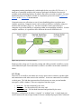
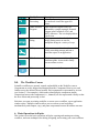
Kepler is a software application for the analysis and modeling of scientific data. Kepler
simplifies the effort required to create executable models by using a visual representation
of these processes. These representations, or “scientific workflows,” display the flow of
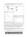
data among discrete analysis and modeling components (Figure 1).
2
Figure 1: A simple scientific workflow developed in Kepler
Kepler allows scientists to create their own executable scientific workflows by simply
dragging and dropping components onto a workflow creation area and connecting the
components to construct a specific data flow, creating a visual model of the analytical
portion of their research. Kepler represents the overall workflow visually so that it is
easy to understand how data flow from one component to another. The resulting
workflow can be saved in a text format, emailed to colleagues, and/or published for
sharing with colleagues worldwide.
Kepler users with little background in computer science can create workflows with
standard components, or modify existing workflows to suit their needs. Quantitative
analysts can use the visual interface to create and share R and other statistical analyses.
Users need not know how to program in R in order to take advantage of its powerful
analytical features; pre-programmed Kepler components can simply be dragged into a
visually represented workflow. Even advanced users will find that Kepler offers many
advantages, particularly when it comes to presenting complex programs and analyses in a
comprehensible and easily shared way.
Kepler includes distributed computing technologies that allow scientists to share their
data and workflows with other scientists and to use data and analytical workflows from
others around the world. Kepler also provides access to a continually expanding,
geographically distributed set of data repositories, computing resources, and workflow
libraries (e.g., ecological data from field stations, specimen data from museum
collections, data from the geosciences, etc.).
3
1.2.
What are Scientific Workflows?
Scientific workflows are a flexible tool for accessing scientific data (streaming sensor
data, medical and satellite images, simulation output, observational data, etc.) and
executing complex analysis on the retrieved data.
Each workflow consists of analytical steps that may involve database access and
querying, data analysis and mining, and intensive computations performed on high
performance cluster computers. Each workflow step is represented by an “actor,” a
processing component that can be dragged and dropped into a workflow via Kepler’s
visual interface. Connected actors (and a few other components that we’ll discuss in later
sections) form a workflow, allowing scientists to inspect and display data on the fly as it
is computed, make parameter changes as necessary, and re-run and reproduce
experimental results.1
Workflows may represent theoretical models or observational analyses; they can be
simple and linear, or complex and non-linear. One of the benefits of scientific workflows
is that they can be nested, meaning that a workflow can contain “sub-workflows” that
perform embedded tasks. A nested workflow (also known as a composite actor) is a reusable component that performs a potentially complex task.
Scientific workflows in Kepler provide access to the benefits of today’s grid technologies
(providing access to distributed resources such as data and computational services), while
hiding the underlying complexity of those technologies. Kepler automates low-level data
processing tasks so that scientists can focus instead on the scientific questions of interest.
Workflows also provide the following:
•
•
•
•
•
documentation of all aspects of an analysis
visual representation of analytical steps
ability to work across multiple systems
reproducibility of a given project with little effort
reuse of part or all of a workflow in a different project
To date, most scientific workflows have involved a variety of software programs and
sophisticated programming languages. Traditionally, scientists have used STELLA or
Simulink to model systems graphically, and R or MATLAB to perform statistical
analyses. Some users perform calculations in Excel, which is user-friendly, but offers no
record of what steps have been executed. Kepler combines the advantages of all of these
programs, permitting users to model, analyze, and display data in one easy-to-use
interface.
1
See Ludäscher, B., I. Altintas, C. Berkley, D. Higgins, E. Jaeger-Frank, M. Jones, E. Lee, J. Tao, Y.
Zhao. 2005. Scientific Workflow Management and the Kepler System, DOI: 10.1002/cpe.994
4
Kepler builds upon the open-source Ptolemy II visual modeling system
(http://ptolemy.eecs.berkeley.edu/ptolemyII/), creating a single work environment for
scientists. The result is a user-friendly program that allows scientists to create their own
scientific workflows without having to integrate several different software programs or
enlist the assistance of computer programmers.
A number of ready-to-use components come standard with Kepler, including generic
mathematical, statistical, and signal processing components and components for data
input, manipulation, and display. R- or MATLAB-based statistical analysis, image
processing, and GIS functionality are available through direct links to these external
packages. You may also create new components or wrap existing components from other
programs (e.g., C programs) for use within Kepler.
2. Downloading and Installing Kepler
Kepler is an open-source, cross-platform software program that can run on Windows,
Macintosh, or Linux-based platforms. Kepler can be downloaded from the project
website: http://kepler-project.org. Kepler 2.0.0 is the most current release.
Kepler releases are a continual work in progress, and Kepler users are encouraged to
contribute to the product by suggest new features that would be of use, as well as to
notify the designers of bugs and other problems. See https://keplerproject.org/developers/get-involved for more information. Community involvement in
the on-going development of Kepler has proved valuable because it allows the system to
quickly adapt to the needs of practicing scientists. To stay abreast of changes and
updates, subscribe to the Kepler users’ mailing list at
http://mercury.nceas.ucsb.edu/ecoinformatics/mailman/listinfo/kepler-users.
2.1.
System Requirements
Recommended system requirements for running Kepler:
•
•
•
•
•
•
300 MB of disk space
512 MB of RAM minimum, 1 GB or more recommended
2 GHz CPU minimum
Java 1.5.x (you may also use Java 1.6)
Network connection (optional). Although a connection is not required to run
Kepler, many workflows require a connection to access networked resources.)
R software (optional). R is a language and environment for statistical computing
and graphics, and it is required for some common Kepler functionality. R is
included with the full Kepler installation for Windows and Macintosh; R is not
included with Kepler's Linux installer.
5
To download and install Kepler, follow the instructions for your system. Downloading
the installer files may be time consuming depending upon your connection.
NOTE: Java 1.5.x or greater is required and can be obtained from Sun’s Java website at:
http://java.sun.com/j2se/downloads/ or from your system administrator. Kepler installers
for Windows and Linux will direct you to a page to download and install Java 1.5.x if it is
not already installed on your system. Check the installation instructions for your platform
for more information.
2.2.
Installing on Windows
The Windows installer will install the Kepler application and (optionally) R--a statistical
computing language and environment used by a number of Kepler actors--on your
system. If you do not have Java 1.5.x installed, the installer will direct you to a page to
download and install it. Java 1.5.x or greater is required in order to run the Kepler
software.
If R is installed with Kepler, it should not interfere with a previously installed version of
R except when one launches R from the command line (by entering 'R'). The Kepler
installer updates your system so that the new version of R will be launched from the
command line. Existing shortcuts will still open the previously installed R application.
The version of R included with the Kepler installer is 2.10.1.
Follow these steps to download and install Kepler for Windows:
1. Click the following link: https://kepler-project.org/users/downloads and select the
Windows installer
2. Save the install file to your computer.
3. Double-click the install file to open the install wizard.
4. Follow the steps presented to complete the Kepler installation process.
Once the installation process is complete, a Kepler shortcut icon will appear on your
desktop (Figure 2) and/or in the Start Menu.
Figure 2: Kepler shortcut icon
2.3.
Installing on Macintosh
The Mac installer will install the Kepler application and (optionally) R--a statistical
computing language and environment used by a number of Kepler actors--on your
system. Java is included as part of the Mac OSX operating system, so it need not be
installed.
6
Because R is required for some common Kepler functionality, we recommend that users
choose to install R with the Kepler installation (the default). If R is installed with Kepler,
it should not interfere with a previously installed version of R except when one launches
R from the command line (by entering 'R'). The Kepler installer updates your system so
that the new version of R will be launched from the command line. Existing shortcuts
will still open the previously installed R application. The version of R included with the
Kepler installer is 2.10.1.
Follow these steps to download and install Kepler for Macintosh systems:
1
2
3
Click the following link: https://kepler-project.org/users/downloads and select the
Mac install file. Save the install file to your computer.
Double-click the install icon that appears on your desktop when the extraction is
complete.
Follow the steps presented in the install wizard to complete the Kepler installation
process.
A Kepler icon is created under Applications/Kepler. The icon can be dragged and
dropped to the desktop or the dock if desired.
2.4. Installing on Linux
The Linux installer will install the Kepler application and, if you do not have Java 1.5.x
installed, direct you to a page to download and install it. Java 1.5.x or greater is required
in order to run the Kepler software.
R, a language and environment for statistical computing and graphics, is NOT included
with the Linux installer. Because R is required for some common Kepler functionality,
we recommend that users download and install R. For more information about R, see
http://www.r-project.org.
Follow these steps to download and install Kepler for Linux:
1. Click the following link: https://kepler-project.org/users/downloads and
select the Linux install file.
2. Save the install file to your computer
3. Double-click the install file to open the install wizard. We recommend that you
quit all programs before continuing with the installation.
4. The Kepler installer displays a status bar as the installation progresses.
3. Starting Kepler
To start Kepler, follow the instructions for your platform.
7
3.1. Windows and Macintosh Platforms
To start Kepler on a PC, double-click the Kepler shortcut icon on the desktop (Figure 2).
Kepler can also be started from the Start menu. Navigate to Start menu > All Programs,
and select "Kepler" to start the application. On a Mac, the Kepler icon is created under
Applications/Kepler. The icon can be dragged and dropped to the desktop or the dock if
desired.
The main Kepler application window opens (Figure 3). From this window you can
access and run sample and existing scientific workflows and/or create your own custom
scientific workflow. Each time you open an existing workflow or create a new workflow,
a new application window will open. Multiple windows allow you to work on several
workflows simultaneously and compare, copy, and paste components between workflows
3.2.
Linux Platform
To start Kepler on a Linux machine, use the following steps:
1. Open a shell window. On some Linux systems, a shell can be opened by rightclicking anywhere on the desktop and selecting "Open Terminal". Speak to your
system administrator if you need information about your system.
2. Navigate to the directory in which Kepler is installed. To change the directory,
use the cd command (e.g., cd directory_name).
3. Type ./kepler.sh to run the application.
The main Kepler application window opens (Figure 2.3). From this window you can
access and run existing scientific workflows and/or create your own custom scientific
workflow. Each time you open an existing workflow or create a new workflow, a new
application window opens. Multiple windows allow you to work on several workflows
simultaneously and compare, copy, and paste components between workflows.
4. Basic Components in Kepler
Scientific workflows consist of customizable components—directors, actors, and
parameters—as well as relations and ports, which facilitate communication between the
components.
8
Figure 3: Main window of Kepler with some of the major workflow components highlighted. The
windows on the bottom right are output windows, created by the workflow to display result graphs.
4.1. Director and Actors
Kepler uses a director/actor metaphor to visually represent the various components of a
workflow. A director controls (or directs) the execution of a workflow, just as a film
director oversees a cast and crew. The actors take their execution instructions from the
director. In other words, actors specify what processing occurs while the director
specifies when it occurs.
Every workflow must have a director that controls the execution of the workflow using a
particular model of computation. Each model of computation in Kepler is represented by
its own director. For example, workflow execution can be synchronous, with processing
occurring one component at a time in a pre-calculated sequence (SDF Director).
Alternatively, workflow components can execute in parallel, with one or more
9
components running simultaneously (which might be the case with a PN Director). A
small set of commonly used directors come pre-packaged with Kepler, but more are
available in the underlying Ptolemy II software that can be accessed as needed. For more
detailed discussion of workflow models of computation, please refer to the Kepler User
Manual or the Ptolemy II documentation.
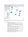
Composite actors are collections or sets of actors bundled together to perform more
complex operations. Composite actors can be used in workflows, essentially acting as a
nested or sub-workflow (Figure 4). An entire workflow can be represented as a
composite actor and included as a component within an encapsulating workflow. In more
complex workflows, it is possible to have different directors at different levels.
Figure 4: Representation of a nested workflow.
Kepler provides a large set of actors for creating and editing scientific workflows. Actors
can be added to Kepler for an individual’s exclusive use and/or can be made available to
others.
4.2. Ports
Each actor in a workflow can contain one or more ports used to consume or produce data
and communicate with other actors in the workflow. Actors are connected in a workflow
via their ports. The link that represents data flow between one actor port and another
actor port is called a channel. Ports are categorized into three types:
•
•
•
input port – for data consumed by the actor;
output port – for data produced by the actor; and
input/output port – for data both consumed and produced by the actor.
Each port is configured to be either a “singular” or “multiple” port. A single input port
can be connected to only a single channel, whereas a multiple input port can be connected
10
to multiple channels. Single ports are designated with a dark triangle; multiple ports use a
hollow triangle.
Workflows can also use external ports and port parameters. See the Ptolemy
documentation for more information.
4.3. Relations
Relations allow users to “branch” a data flow. Branched data can be sent to multiple
places in the workflow. For example, a scientist might wish to direct the output of an
operational actor to another operational actor for further processing, and to a display actor
to display the data at that specific reference point. By placing a Relation in the output
data channel, the user can direct the information to both places simultaneously.
4.4. Parameters
Parameters are configurable values that can be attached to a workflow or to individual
directors or actors. For example, the Integrator actor has a parameter called
InitialState that should be set to the initial value of the function being integrated.
The parameters of simulation model actors can be configured to control certain aspects of
the simulation, such as initial values. Director parameters control the number of
workflow iterations and the relevant criteria for each iteration.
The next sections provide an overview of the interface and step-by-step examples of how
to open, edit, and run different scientific workflows.
5. Kepler Interface
Scientific workflows are edited and built in Kepler’s easily navigated, drag-and-drop
interface. The major sections of the Kepler application window (Figure 5) consist of the
following:
•
•
•
•
•
Menu bar – provides access to all Kepler functions.
Toolbar – provides access to the most commonly used Kepler functions.
Components and Data Access area – consists of a Components tab , Data tab, and
an Outline tab. The Components tab and the Outline tab both contain a search
function and display the library of available components and/or search results.
Workflow canvas – provides space for displaying and creating workflows.
Navigation area – displays the full workflow. Click a section of the workflow
displayed in the Navigation area to select and display that section on the
Workflow canvas.
11
Figure 5: Empty Kepler window with major sections annotated.
5.1.
The Toolbar
The Kepler toolbar is designed to contain the most commonly used Kepler functions
(Figure 6).
The main sections of the toolbar include:
• Viewing –zoom in, reset, fit, and zoom out of the workflow on the Workflow
canvas
• Run – run, pause, and stop the workflow without opening the Run window
• Ports – add single (black) or multi (white) input and output ports to workflows;
add Relations to workflows
12
Figure 6: Annotated Kepler Toolbar
5.2.
Components, Data Access, and Outline Area
The Components, Data Access, and Outline area contains a library of workflow
components (e.g., directors and actors, under the Components tab), a search mechanism
for locating and using data sets (under the Data tab), and an outline view of the workflow
(under the Outline tab). When the application is first opened, the Components tab is
displayed.
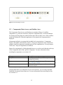
Components in Kepler are arranged in four high-level categorizations: Components,
Projects, Disciplines, and Statistics (Table 1). Any given component can be classified in
multiple categories, appearing in multiple places in the component tree. Use any instance
of the actor—only its categorization is different.
Browse for components by clicking through the trees, or use the search function at the top
of the Components tab to find a specific component. For more information about
searching for components, see section 6.4.2.
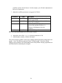
Category
Components
Description
Contains a standard library of all components,
arranged by function.
Projects
Contains a library of project-specific components
(e.g., SEEK or CIPRes)
Contains a library of components for use with
statistical analysis.
Statistics
Table 1: Component Categories in Kepler
Click the Data tab to reveal the Data Access area. From here, you can easily search the
EarthGrid for remotely hosted data sets. For more information about searching for data,
see section 6.4.1.
13
5.3.
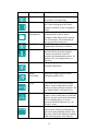
Director and Actor Icons
In Kepler, icons provide a visual representation of each component’s function. Directors
are represented by a single icon; actors are divided into functional categories, or families,
with each category assigned a visually related icon (Table 2).
Some actor families have a persistent family symbol, other families do not. The majority
of the actor icons use a teal rectangle, though some icons, such as the Data/File Access
icons use other colors and/or shapes. In the table below, persistent symbols are noted. For
families that do not have a persistent symbol, an example of one of the icons from that
family is displayed. A table that includes all icons for each family can be found in
Chapter 5 of the Kepler User Manual.
Icon
Family Name
Director
Description
Stand-alone component that directs the
other components (the actors) in their
execution
Array
Array actors are indicated with a curly
brace. Actors belonging to this family are
used for general array processing (e.g.,
array sorting).
Composite actors are represented by
multiple teal rectangles because they
represent multiple actors. Composite
actors are collections of actors bundled
together to perform more complex
operations (i.e., subworkflows) within an
encapsulating workflow.
Control actors do not have a persistent
family symbol. These actors are used to
control workflows (e.g., stop, pause, or
repeat).
Data/File Access actors do not have a
persistent family symbol. Actors
belonging to this family read, write, and
query data. The icon displayed here is a
data write icon.
Composite
Control
Data/File
Access
14
Icon
Family Name
Description
Data Processing
Data Processing actors assemble,
disassemble, and update data.
Display
Display actors are indicated by vertical
bars. Actors belonging to this family
output the workflow in text or graphical
format
File
Management
File Management actors do not have a
persistent family symbol. Actors
belonging to this family locate or unzip
files, for example. The icon displayed
here is a directory listing icon.
GAMESS actors are used for
computational chemistry workflows.
GAMESS
General
GIS/Spatial
Actors that don't fit into one of the other
families fall into the General family.
General actors include email, file
operation, and transformation actors, for
example. The icon displayed here is a
filter icon.
GIS/Spatial actors are used to process
geospatial information
Image
Processing
Image Processing actors are used to
manipulate graphics files.
Logic
Logic actors have no persistent family
symbol. Actors in this family include
Boolean switches and logic functions. The
icon displayed here is an equals icon.
Math
Math actors have no persistent family
symbol. Actors in this family include add,
subtract, integral, and statistical functions.
The icon displayed here is used to
represent statistical functions (e.g., the
Quantizer actor).
Model actors use a solid arrow. Model
actors include statistical, mathematical,
rule-based, and probability models. Note
that icons will include additional symbols
further identifying the actor function.
Model
15
Icon
Family Name
Molecular
Processing
Other/External
Program
String
Description
Molecular Processing actors are indicated
by a molecule icon in the upper left
corner.
Other/External Program actors are
indicated by a purple rectangle. External
Program actors include R, SAS, and
MATLAB actors. The icon displayed here
is an R icon.
String actors are indicated with the text
string().String actors are used to
manipulate strings in a variety of ways
Utility
Utility actors are indicated with a wrench.
Utility actors help manage and tune a
particular aspect of an application.
Web Services
Web Services actors are indicated by a
wireframe globe. Actors in this family
execute remote services.
Units
Unit components define a system of units.
Table 2: The major Kepler icons
5.4.
The Workflow Canvas
Scientific workflows are opened, created, and modified on the Workflow canvas.
Components are easily dragged and dropped from the Component, Data Access, and
Outline area to the desired canvas location. Each component is represented by an icon
(see Section 5.3 for examples), which makes identifying the components simple.
Connections between the components (i.e., channels) are also represented visually so that
the flow of data and processing is clear.
Each time you open an existing workflow or create a new workflow, a new application
window opens. Multiple windows allow you to work on several workflows
simultaneously and compare, copy, and paste components between Workflow canvases.
6. Basic Operations in Kepler
This section covers the basic operations in Kepler: opening and running an existing
workflow, and some techniques for editing, designing, and creating your own workflows.
16
6.1. Opening an Existing Scientific Workflow
To open any existing workflow:
1. From the Menu bar, select File, then Open File. A standard file dialog box will
appear.
2. If the file dialog box does not open to the “kepler” directory (the place where the
Kepler program is installed), then navigate to that directory. Workflows discussed
in this guide are stored in Kepler's "/demos/getting-started" directory.
3. Double-click a workflow file to open it. The workflow will appear in the
Workflow canvas of the application window.
Note: All demo workflows in Kepler 2.0.0 are located in your home directory under the
KeplerData directory.
6.1.1. Example 1: Opening the Lotka-Volterra Workflow
In this example we will open a specific workflow: the classic predator pray model, the
Lotka-Volterra workflow. To open this workflow:
17
1. From the Menu bar, select File, then Open File. A standard file dialog box will
appear.
2. Navigate to Kepler's "/demos/getting-started" directory and locate the file named
“02-LotkaVolterraPredatorPrey.xml” (Figure 7).
Figure 7: Navigating to the Lotka-Volterra workflow. The workflow is in Kepler's “/demos/gettingstarted” directory.
3. Double-click the “02-LotkaVolterraPredatorPrey.xml” file. The Lotka-Volterra
workflow appears in the Workflow canvas of the application window (Figure 8).
18
Figure 8: The Lotka-Volterra workflow in the Kepler interface.
6.2. Running an Existing Scientific Workflow
To run any existing scientific workflow:
1. Open the desired workflow.
2. From the Toolbar, select the Run button. (
)
3. The workflow will execute and produce the specified output.
OR
1. Open the desired workflow.
2. From the Menu bar, select Workflow, then Runtime Window. A Run window
will appear (Figure 9). If the workflow has parameters, they will appear here.
3. Adjust the parameters as needed, and then click the Go button.
4. The workflow will execute and produce the specified output. During workflow
execution, you may select the Pause, Resume, or Stop buttons.
19
Figure 9: The Runtime window, displaying the Lotka-Volterra workflow. Click the Go button to run the
workflow. Director and model parameters can be edited in the Runtime window. Output is displayed in the
window as well.
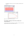
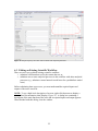
6.2.1. Example 2: Running the Lotka-Volterra Workflow with Default
Parameters
The Lotka-Volterra model uses the continuous time domain (i.e., a CT Director) in
Kepler to solve two coupled differential equations: one that models the predator
population; and one that models the prey population. The results are plotted as they are
calculated, showing both populations change and a phase diagram. For more information
about the model, see Section 6.2.2.
To run the Lotka-Volterra workflow:
1. Open the workflow file named “02-LotkaVolterraPredatorPrey” from Kepler's
“/demos/getting-started/” directory.
2. From the Menu bar, select Run.
3. The Lotka-Volterra workflow will execute with the default parameters and
produce two graphs. The graph labeled TimedPlotter depicts the interaction of
predator and prey over time (i.e., the cyclical changes of the predator and prey
populations over time predicted by the model). The graph labeled XYPlotter
depicts a phase portrait of the population cycle (i.e., the predator population
against the prey population). Together these graphs show how the predator and
20
prey populations are linked: as prey increases, the number of predators increase.
(Figure 10)
Figure 10: Graphs output by the Lotka-Volterra workflow
6.2.2. Example 3: Running the Lotka-Volterra Workflow with
Adjusted Parameters
To better illustrate the effect of parameters on a workflow, we must first provide some
background about the Lotka-Volterra workflow (Figure 11).
21
Figure 11: Graphic of Lotka-Volterra workflow
The Lotka-Volterra model was developed independently by Lotka (1925)2 and Volterra
(1926)3 and is made up of two differential equations. One describes how the prey
population changes (dn1/dt = r*n1 - a*n1*n2), and the second equation describes how the
predator population changes (dn2/dt = -d*n2 + b*n1*n2).
The Lotka-Volterra model is based on certain assumptions:
• the prey has unlimited resources;
• the prey's only threat is the predator;
• the predator is a specialist (i.e., the predator's only food supply is the prey); and
• the predator's growth depends on the prey it catches
The Lotka-Volterra model as represented in Kepler as a scientific workflow contains:
• six actors - two plotters, two equations, and two integral functions;
• one director; and
2
Lotka, Alfred J (1925). Elements of physical biology. Baltimore: Williams & Williams Co.
3
Volterra, Vito (1926) Fluctuations in the abundance of a species considered mathematically. Nature 118.
558-560.
22
•
four workflow parameters (Table 3).
NOTE: The director of the Lotka_Volterra model has several configurable parameters as
do the two plotter actors.
The critical assumptions above provide the basis for the workflow parameters. The
workflow parameters and their defaults are as follows:
Parameter
r
Default
Value
2
a
0.1
b
0.1
d
0.1
Description
the intrinsic rate of growth of prey in the absence
of predation
capture efficiency of a predator or death rate of
prey due to predation
proportion of consumed prey biomass converted
into predator biomass (i.e., efficiency of turning
prey into new predators)
death rate of the predator
Table 3: Description of the default parameters for the Lotka-Volterra workflow
In the differential equations used in the workflow, (dn1/dt = r*n1 - a*n1*n2) and (dn2/dt
= -d*n2 + b*n1*n2), the variable n1 represents prey density, and the variable n2
represents predator density.
When changing parameters in a workflow, the assumptions of the model must be kept in
mind. For example, if creating a Lotka-Volterra model with rabbits as prey and foxes as
predators, the following assumptions can be made with regard to how the rabbit
population changes in response to fox population behavior:
•
•
•
•
•
the rabbit population grows exponentially unless it is controlled by a predator;
rabbit mortality is determined by fox predation;
foxes eat rabbits at a rate proportional to the number of encounters;
the fox population growth rate is determined by the number of rabbits they eat and
their efficiency of converting the eaten rabbits into new baby foxes; and
fox mortality is determined by natural processes.
If you think of each run of the model in terms of the rates at which these processes would
occur, then you can think of changing the parameters in terms of percent of change over
time.
To run the Lotka-Volterra workflow with adjusted parameters:
1. Open the workflow file named “02-LotkaVolterraPredatorPrey” from Kepler's
“/demos/getting-started” directory
2. From the Menu bar, select Workflow, then Runtime Window. The Runtime
window will appear. Notice there are two sets of parameters – one for the
23
workflow and one for the director. In this example, you will make adjustments to
both sets of parameters.
3. Adjust the workflow parameters as suggested in Table 4.
Parameter
r
Value
0.04
a
0.0005
b
0.1
d
0.2
Description
the intrinsic rate of growth of prey in the
absence of predation
capture efficiency of a predator or death rate
of prey due to predation
proportion of consumed prey biomass
converted into predator biomass (i.e.,
efficiency of turning prey into new
predators)
death rate of the predator
Table 4: Description of the suggested parameters for the Lotka-Volterra workflow taken from
http://www.stolaf.edu/people/mckelvey/envision.dir/lotka-volt.html
4. Adjust the value of the stopTime director parameter to 300.
5. In the Runtime window, click the Go button.
The Lotka-Volterra workflow will execute with the adjusted parameters and produce two
graphs: 1) the TimedPlotter graph and 2) the XYPlotter graph. Note that with the
changes in the parameters, the relationship between the predator and prey populations are
still linked but the relationship has changed.
24
Figure 12: Graphs output by the Lotka-Volterra model with adjusted parameters
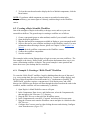
6.3. Editing an Existing Scientific Workflow
There are two ways to edit an existing scientific workflow:
• substitute a different data set for the current data set; or
• substitute one or more analytical processes in the workflow with other analytical
processes (e.g., substitute a neural network model actor for a probabilistic model
actor).
Before substituting data or processes, you must understand the required inputs and
outputs of the actors involved.
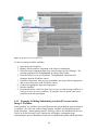
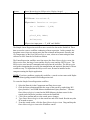
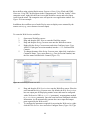
NOTE: To see a high-level description of an actor, right-click that actor to display a
menu; select Documentation, then Display (Figure 13). A dialog box containing a
description of the main function of the actor and its required inputs and output appears.
When finished with this dialog, close the window.
25
Figure 13: Displaying actor documentation
To edit an existing scientific workflow:
1. Open the desired workflow.
2. Identify which workflow component is the target for substitution.
3. Select the target component (data actor or processing actor) by clicking it. The
selected component will be highlighted in a thick yellow border.
4. Press the Delete key on your keyboard. The highlighted component will
disappear from the Workflow canvas.
5. From the Components, Data Access, and Outline area, drag either an appropriate
data or processing actor to the Workflow canvas.
6. Connect the appropriate input and output ports.
7. Run the workflow.
8. From the Menu bar, select File, then Save (to save over the existing workflow) or
Save As (to save as a new workflow). If using the Save As option, enter a new
workflow name when prompted.
6.3.1. Example 4: Editing/Substituting Analytical Processes in the
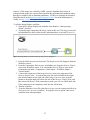
Image J Workflow
In this example, we will show how two different actors can perform the same function in
a workflow. We will work with the Image Display workflow (03-ImageDisplay.xml)
found in Kepler's “/demos/getting-started/” directory, and we will substitute the Browser
Display actor for the ImageJ actor. Both actors will display a bitmapped image
representing the species distribution of the species Mephitis throughout North and South
26
America. (This image was created by GARP, a genetic algorithm that creates an
ecological niche model for a species that represents the environmental conditions where
that species would be able to maintain populations. GARP was originally developed by
David Stockwell, at the San Diego Supercomputer Center. For more information on
GARP, see http://www.lifemapper.org/desktopgarp/.)
To edit the Image Display workflow:
1. Open the 03-Image-Display.xml workflow from Kepler's “/demos/gettingstarted/” directory.
2. Select the target component, the ImageJ actor in this case. The ImageJ actor will
be highlighted in a thick yellow border, indicating that it is selected (Figure 14).
Figure 14: Image Display workflow showing ImageJ actor highlighted
3. Press the Delete key on your keyboard. The ImageJ actor will disappear from the
Workflow canvas.
4. From the Components, Data Access, and Outline area, drag the Browser Display
actor to the Workflow canvas. You can find the Browser Display actor in the
Components tab under “Components > Data Output > Workflow Output >
Textual Output.”
5. Connect the output port of the ImageConverter actor to the input port of the
Browser Display actor. To connect the ports, left-click and hold on the output
port (black triangle) on the right side of the Image Converter actor, drag the
pointer to the upper input port on the left side of the Browser Display actor, and
then release the mouse. If the connection is made, you will see a thick black line.
If the connection is not completely made, the line will be thin.
6. Run the workflow.
7. From the Menu bar, select File, then Save (to save over the existing workflow) or
Save As (to save as a new workflow). If using the Save As option, enter a new
workflow name when prompted.
27
Figure 15: The Image Display workflow with the Browser Display actor substituted for the ImageJ actor.
NOTE: Sometimes the easiest way to connect actors is to go from the output port of the
source to the input port of the destination.
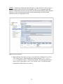
6.4. Searching in Kepler
Kepler provides a searching mechanism to locate data (on the EarthGrid) and analytical
processing components (on the local system or both the local system and a remote
component repository). The examples given in this section describe searching for data
and components in Kepler.
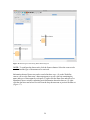
6.4.1. Searching for Available Data
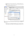
Via its search capabilities, Kepler provides access to data from the EarthGrid. EarthGrid
resources are stored in the KNB Metacat http://knb.ecoinformatics.org and the KU Digir
http://www.specifysoftware.org/Informatics/informaticsdigir/ databases. To search for
data on the EarthGrid through Kepler:
1. In the Components, Data Access and Outline area, select the Data tab (Figure 16).
2. Type in the desired search string (e.g., Datos Meteorologicos). Make sure that the
search string is spelled correctly. (You can also enter just part of the entire string
– e.g. ‘Datos’)
3. Click the Search button. The search may take several moments. You may be
prompted for log in credentials. If so, enter your user and password information,
or click "Login Anonymously." When the search is complete, a list of search
results (i.e., Data actors) will be displayed in the Components and Data Access
area.
4. To use one or more data actors in a workflow, simply drag the desired actors to
the Workflow canvas.
28
Figure 16: Searching for and locating Datos Meteorologicos
NOTE: To configure the data search, click the Sources button. Select the sources to be
searched and the type of documents to be retrieved.
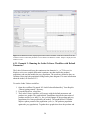
Information about a Data actor can be revealed in three ways: (1) on the Workflow
canvas, roll over the Data actor’s data output ports to reveal a tool tip containing the
name and type of data output by each port; (2) right-click the Data actor and select Get
Metadata to open a window containing more information about the data set; (3) rightclick the data actor and select Preview from the drop-down menu to preview the data set
(Figure 17).
29
Figure 17: Previewing a data set.
6.4.2. Searching for Available Processing Components
Kepler comes standard with over 350 workflow components and the ability to modify
and create your own. You can create an innumerable number of workflows with a variety
of analytic functions. The default set of Kepler processing components is displayed
under the Components tab in the Components and Data Access area. Components are
organized by function (e.g., “Director” or “Filter Actor”). To search for components:
1. In the Components and Data Access area to the left of the Workflow canvas,
select the Components tab.
2. Type in the desired search string (e.g., “File Copy”).
3. Click the Search button. When the search is complete, the search results are
displayed in the Components and Data Access area. The search results replace the
default list of components. You may notice multiple instances of the same
component (Because components are arranged by category, the same component
may appear in multiple places in the search results.)
4. To use one or more processing components in a workflow, simply drag the
desired components to the Workflow canvas.
30
5. To clear the search results and re-display the list of default components, click the
Reset button.
NOTE: If you know which component you want to use and its location in the
Component library, you can navigate to it directly, and then drag it to the Workflow
canvas.
6.5. Creating a Basic Scientific Workflow
One of the strengths of Kepler is the ability to design, create, and save your own
executable workflows. The general steps in creating a workflow are as follows:
1.
2.
3.
4.
Create a conceptual (paper or other medium) model of your scientific workflow.
Open the Kepler application.
Map the data and actor components available in Kepler to your conceptual model.
Select a director for your workflow and drag it to the Workflow canvas. For more
information about choosing a director, please see Chapter 5 of the Kepler User
Manual.
5. Drag the desired workflow components to the Workflow canvas.
6. Connect the workflow components.
7. Save the workflow.
The examples in this section illustrate how to begin to create your own workflows. The
first example is the classic “Hello World” workflow that demonstrates how easy it is to
create a functioning workflow in Kepler. The second example is more practical and
shows how to use your desktop data in a workflow.
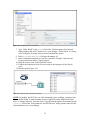
6.5.1. Example 5: Creating a “Hello World” Workflow
To create the “Hello World” workflow, begin by thinking about the type of data used
(e.g., text or string data); the type of output desired (e.g., textual or image display); and
the type of director needed to execute this model (e.g., synchronous or parallel) The
“Hello World” workflow requires a constant actor, a text display actor, and a SDF
director (in a SDF director, the data will flow through the actors based on the order in the
workflow, and the workflow will run continuously, by default).
1. Open Kepler. A blank Workflow canvas will open.
2. In the Components, Data Access, and Outline area, select the Components tab,
then navigate to the “Directors-2_0” directory.
3. Drag the SDF Director to the top of the Workflow canvas.
4. In the Components tab, search for “Constant” and select the Constant actor.
5. Drag the Constant actor onto the Workflow canvas and place it a little below the
SDF Director.
6. Configure the Constant actor by right-clicking the actor and selecting Configure
Actor from the menu. (Figure 18)
31
Figure 18: Configuring the Constant actor.
7. Type “Hello World” in the value field of the “Edit parameters for Constant”
dialog window and click Commit to save your changes. “Hello World” is a string
value. In Kepler, all string values must be surrounded by quotes.
8. In the firingCountLimit field type the number 10.
9. In the Components and Data Access area, search for “Display” and select the
Display actor found under “Textual Output.”
10. Drag the Display actor to the Workflow canvas.
11. Connect the output port of the Constant actor to the input port of the Display
actor.
12. Run the model (Figure 19).
Figure 19: “Hello World” workflow and output.
NOTE: By default, the SDF Director will continuously run a workflow, creating a loop.
To run “Hello World” a limited number of times, right-click on the SDF Director and
select “Configure Director” from the menu. Type the desired number of iterations into the
iterations field of the “Edit parameters for SDF Director” dialog window and click the
Commit button to save your changes.
32
6.5.2. Example 6: Creating a Simple Workflow Using Local Data
In this example, we create a simple workflow using an actor that reads a local data file
containing information about species abundance and then sends the data to a second actor
for display.
Kepler can read data in many ways and from many formats. In this example, we will use
an actor to review a data table. To determine which actor is appropriate, consider the
format in which the data are saved. In this example, the data are saved in a text format.
As such we will use the File Reader actor to read the data in a tabular format. This
workflow requires two actors: a File Reader actor and a Display actor to output text. In
addition, the example requires a SDF Director.
1. From the Menu bar, select File, then New Workflow, and then Blank. A new
window will open with a blank Workflow canvas.
2. In the Components, Data Access and Outline area, select the Components tab, and
then navigate to the “Directors-2_0” directory.
3. Drag the SDF Director to the top of the Workflow canvas.
4. In the Components tab, type “File Reader” in the Search box, then click the
Search button.
5. Drag the File Reader actor to the Workflow canvas.
6. Right-click the File Reader actor and select Configure Actor from the menu. An
“Edit parameters for File Reader” dialog window will open.
7. Click the Browse button to the right of the fileOrURL parameter and navigate
to the following file: mollusc_abundance.txt. These data come installed in Kepler
and are located in Kepler's "/demos/getting-started/" directory (Figure 20).
8. In the firingCountLimit field type the number 1.
33
Figure 20: Configuring the File Reader actor to use data from your local machine.
9. Click the Commit button at the bottom of the “Edit Parameters for File Reader”
dialog box. The actor is now configured to read the specified file.
10. In the Components tab, search for “Display”. Select the Display actor and drag it
onto the Workflow canvas to the right of the File Reader actor.
11. Connect the output port of the File Reader actor to the input port of the Display
actor.
12. From the Toolbar, select the Run button. A pop-up window will appear,
displaying the contents of the data file in tabular format (Figure 21).
13. From the Menu bar, select File, then Save. When prompted, save the newly
created workflow to the Kepler “demos/getting-started” directory with the name
“readingdata.xml.”
Figure 21: Using and displaying local data in a workflow.
34
NOTE: When creating a workflow, remember that the limitations of the data determine
which processing components are appropriate.
7. Sample Scientific Workflows
This section examines a small set of sample scientific workflows that come standard with
Kepler, and provides step-by-step instructions for creating these workflows.
7.1.
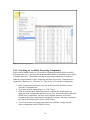
Sample Workflow 1 – Simple Statistics
Name
File name
Detailed
Description
Assumptions
Director
Data
Actors
Parameters
Summary Statistics
/kepler/demos/getting-started/00-StatisticalSummary.xml
This workflow calculates the mean, standard deviation, and variance of
a set of numerical values. The Constant actors contains the input data:
an array of values {1,2,3,4,5,6,7,8,9,10}. These data are sent to the
SummaryStatistics actor, which calculates the statistics and then outputs
the results through its output ports. Results are displayed by three
TextDisplay actors.
The SummaryStatistics actor is a special adaptation of the RExpression
actor. To run this workflow R, a language and environment for
statistical computing, must be installed on the computer running the
Kepler application.
SDF Director
Data is generated in the Constant actor
Constant, SummaryStatistics, Display
SDF Director: iterations=1
Constant: value= {1,2,3,4,5,6,7,8,9,10}
The Summary Statistics workflow takes a list of numbers, calculates the mean, variance
and standard deviation, and displays the results. This workflow highlights the ease and
functionality of Kepler. To run this workflow R, a language and environment for
statistical computing, must be installed on the computer running the Kepler
application. R is included with the full Kepler installation for Windows and Macintosh; R
is not included with Kepler's Linux installer. To create this workflow, open a new blank
workflow from the File menu (File > New Workflow > Blank) and follow the steps
below:
1. In the Components and Data Access area, select the Components tab.
2. Search for the SDF Director and drag and drop the director to the Workflow
canvas.
35
3. Configure the SDF Director by right-clicking the director and selecting Configure
Director. In the “Edit Parameters for SDF Director” window, set the
iterations parameter to 1 and click Commit.
4. Search for the Constant actor and drag and drop that to the Workflow canvas. The
Constant actor can be found under Components > Data Input > Workflow Input >
Constant.
5. Configure the Constant actor by right-clicking the actor and selecting Configure
Actor. In the “Edit Parameters for Constant” window, set the value field to
{1,2,3,4,5,6,7,8,9,10} and in the firingCountLimit field, set the value to 1,
then click Commit. Note: The braces are needed. Curly braces designate an array
in Kepler.
6. Search for the SummaryStatistics actor and drag and drop it to the Workflow
canvas.
7. Locate the correct output ports of the SummaryStatistics actor by right-clicking
the actor and selecting Configure Ports (Figure 22).
8. In the “Configure ports for SummaryStatistics” dialogue box, under the Show
Name column, click the check box for xmean, xstd, and xvar. Click Commit to
save your changes. The port names for the xmean, xstd and xvar outputs will now
display on the Workflow canvas, making it easier to connect the proper ports.
Figure 22: Displaying port names
9. Connect the output of the Constant actor to the input port of the
SummaryStatistics actor.
10. Search for the text Display actor, and drag and drop that to the Workflow canvas
three times. Note the second actor is named Display2 and the third actor is named
Display3.
11. Customize the name for the three text Display actors by right-clicking each and
selecting Customize Name. In the “Rename Text Display” dialogue box for the
Display actor, type “Mean” and click Commit to save your changes. Name the
Display2 actor "Variance" and the Display3 actor “Standard Deviation”.
12. Connect the xmean, xstd, and xvar output ports of the SummaryStatistics actor to
the input port on the corresponding Mean, Standard Deviation, and Variance
actors.
36
You are now ready to run the workflow. The resulting workflow and output are
displayed in Figure 23.
Figure 23: The Simple Statistics workflow and its output
The right-hand windows in Figure 23 display the mean, variance, and standard deviation
of the data set created by the array of values in the Constant actor. Change the input array
of the Constant actor (for example, try {1,17,6,4,12}) to calculate a new set of
corresponding statistics.
7.2.
Sample Workflow 2 –Linear Regression
Name
File name
Detailed
Description
Simple Linear Regression workflow using R
/kepler/demos/getting-started/05-LinearRegression.xml
This workflow performs a simple linear regression analysis using the
RExpression actor. The workflow creates a scatter plot of the two
variables from the Datos Meteorologicos data set and adds a regression
line using the Y = a + bX equation, where X is the explanatory variable
and Y is the dependent variable. The slope of the line is b, and a is the
intercept (the value of y when x = 0).
Assumptions A linear regression assumes linearity, independence, homoscedasticity,
and normality R must be installed on the system running the workflow. R
is included with the full Kepler installation for Windows and Macintosh.
Director
SDF Director
Data
Datos Meteorologicos
37
Actors
Parameters
Datos Meteorologicos, RExpression, Display, ImageJ
Datos Meteorologicos: Data Output Format = As Column Vector
SDF Director: iterations = 1;
RExpression: R function or script =
res <- lm(BARO ~ T_AIR)
res
plot(T_AIR, BARO)
abline(res);
RExpression: input ports = ‘T_AIR’ and ‘BARO.’
The Simple Linear Regression workflow runs a search for data on the EarthGrid. These
data are used to create a workflow conducting a linear regression. In this example, the
input data comes from two output ports (the data columns on Barometric Pressure and
Air Temperature) of the Datos Meteorologicos actor, a data set of meteorological data
collected in 2001 from the La Hechicera station.
The Linear Regression workflow uses four actors (the Datos Meteorologicos actor, the
RExpression actor, the ImageJ actor and the Display actor) and the SDF Director. The
RExpression actor inserts R commands and scripts into the workflow. The RExpression
actor makes integrating the powerful data manipulation and statistical functions of R into
workflows easy. To implement the RExpression actor, R must be installed on the
computer running the Kepler application.
NOTE: If you have problems creating this workflow, a stored version comes with Kepler
at kepler/demos/getting-started/05LinearRegression.xml.
To create the Simple Linear Regression workflow:
1. Select the Data tab in the Components and Data Access area.
2. Click the Sources button and limit the scope of the search by unchecking “KU
Query Interface” and “KNB Metacat Authenticated Query Interface.” Because
Datos Meteorologicos is stored on the KNB Metacat, the data source for the
search can be limited to just those nodes on the EarthGrid.
3. Click Ok to confirm and save the search source changes.
4. Type Datos Meteorologicos in the search box and click Search. Results may take
20 seconds to return.
5. From the search results, click the Datos Meteorologicos icon. Drag and drop the
Datos Meteorologicos actor to the Workflow canvas.
38
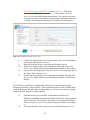
NOTE: To find more information about the data set, right-click Datos Meteorologicos
on the Workflow canvas and select Get Metadata (Figure 24). Depending upon the
amount of information entered by the provider, much valuable metadata can be obtained.
The type of value and measurement type of each attribute help you decide which
statistical models are appropriate to run.
Figure 24: Viewing Metadata
5. Right-click the Datos Meteorologicos actor and select Configure Actor. Select
“As Column Vector” from the pull-down menu beside the Data Output
Format parameter (Figure 25) and click Commit. (The data type of the Datos
Meteorologicos actor must be set to “As Column Vector” to match the input
requirements of the RExpression actor.)
39
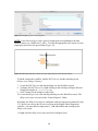
Figure 25: Configuring Datos Meteorologicos
NOTE: Datos Meteorologicos has a series of output ports corresponding to the data
attribute names (e.g., BARO and T_AIR). To locate the appropriate port, mouse-over the
output ports and review the port tooltips (Figure 26).
Figure 26: Identifying data ports. Mouse-over each output port to review the port tooltips.
To finish creating the workflow, add the SDF Director and the remaining actors
(RExpression, ImageJ, Display).
7. Locate the SDF Director and drag and drop it to the Workflow canvas.
8. Configure the SDF Director by right-clicking it and selecting Configure Director
Change the number of iterations to 1.
9. Click Commit for the changes to take effect.
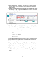
10. Locate the RExpression actor and drag and drop it to the Workflow canvas. The
RExpression actor is located in the “General Purpose” folder.
By default, the RExpression actor is configured with two output ports and the R script
2+2. Before you can use the RExpression actor in the Simple Linear Regression
workflow, you must add two input ports (T_AIR and BARO) and reconfigure the
RExpression script.
11. Right-click the RExpression actor and select Configure Ports.
40
12. In the “Configure ports” dialogue box, click Add twice to add two new ports.
Designate the new ports as input ports by clicking the checkbox named Input
beside each port.
13. Name the new input ports by double-clicking the blank box in the Name column.
Add the name “T_AIR” for one input and “BARO” for the other. Click Commit
to save the changes (Figure 27).
Figure 27: Adding and customizing ports
14. To configure the R script, right-click the RExpression actor and select Configure
Actor. In the “R function or script” dialogue box, change the value of the R
function or script from the default to the following:
res <- lm(BARO ~ T_AIR)
res
plot(T_AIR, BARO)
abline(res)
The above R function tells the RExpression actor to read the Barometric Pressure
and Air Temperature data and then plot the values along with a regression line.
Click Commit to save your changes.
15. Drag and drop the text Display actor to the Workflow canvas. The Display actor
is located under “Components> Data Output > Workflow Output > Textual
Output.”
16. Connect the lower output port of the RExpression actor to the input port of the
Display actor.
17. Drag and drop the ImageJ actor to the Workflow canvas. The ImageJ actor is
located under “Components > Data Output > Workflow Output > Graphical
Output.”
41
Connect the upper output port of the RExpression actor to the input port of the
ImageJ actor. You are now ready to run the workflow. The resulting workflow and
graphic output are shown below (Figure 28).
Figure 28: Linear Regression workflow and its output
The left-hand window in Figure 28 displays the scatter plot of Barometric pressure to Air
Temperature along with a regression line. The graph shows a strong negative relationship
between the two: as air temperature lowers, the Barometric pressure rises. The righthand window displays the Barometric Pressure and Air Temperature data used in the
scatter plot. Additionally, the intercept on the Y-axis (958.38 Barometric Pressure and
the slope – 0.32 for the linear regression equation y=mx+b) is displayed.
You can change the data type and the data set that is run through the workflow. When
changing the data, remember to make sure that the data meets the assumptions mentioned
in workflow table at the beginning of Section 7.2.
7.3.
Sample Workflow 3 – Web Services and Data Transformation
Name
File name
Web Services and Data Transformation Workflow
06-WebServicesAndDataTransformation.xml
42
Detailed
Description
Assumptions
Director
Data
Actors
Parameters
This workflow uses the remote genomics data service to
retrieve a genetic sequence for a given gene accession
number. The sequence is then displayed in three different
ways after appropriate transformations: first in its native
format (XML), second as a sequence of elements
extracted from the XML format, and third as an HTML
document that can be used for display on a website. The
later two operations are performed using composite
actors that hide some of the complexity of the underlying
operations. Composite actors can be thought of as “subworkflows” that execute a potentially complex set of
tasks with a single actor.
The Web Service actor assumes that the target Web
service is RPC-based and uses primitive XML types and
arrays.
SDF Director
The data consists of an initial input gene accession
number that is specified by the String Constant actor and
an intermediate input retrieved from the remote genomics
data service.
String Constant, Display, Sequence Getter Using XPath,
HTML Generator Using XSLT, Web Services,
Web Services:
wsdlUrl=http://xml.nig.ac.jp/wsdl/DDBJ.wsdl
Web Services: methodName=getXMLEntry
The Web Services and Data Transformation workflow uses the Web Service actor to
access a genomics database and return a genetic sequence from it, which is queried using
a remote genomics data service. The name of the returned genetic sequence (i.e., the gene
accession number) is passed to the Web Services actor by a String Constant actor. The
Web Service actor must be configured to access the appropriate remote server. Once
configured, the Web Service actor outputs the gene sequence obtained from the remote
server so that it can be displayed in multiple formats using three different textual Display
actors: one for XML (the format in which the results are returned by default), one for a
sequence of elements extracted from the XML, and one for an HTML document that can
be displayed on a website.
A Relation is used to “branch” the data output by the Web Service actor so that it can be
shared by all of the necessary components.
The workflow uses two composite actors: Sequence Getter Using XPath and HTML
Generator Using XSLT to process the returned XML data and convert it into a sequence
of elements and an HTML file, respectively. These actors have been created for use with
43
this workflow using existing Kepler actors. Sequence Getter Using XPath and HTML
Generator Using XSLT do not appear in the Components tab. To see the “insides” of the
composite actors, right-click the actor icon on the Workflow canvas and select Open
Actor from the menu. The composite actor will open in a new application window. See
Figure 32 for an example.
In addition, the workflow uses a fourth Display actor to display errors returned by the
remote server (e.g., server down or incorrect input).
To create the Web Services workflow:
1.
2.
3.
4.
5.
Open a new Workflow canvas.
Drag and drop the SDF Director onto the Workflow canvas.
Drag and drop the String Constant actor onto the Workflow canvas.
Right-click the String Constant actor and select Configure Actor. Type
AA045112 (the gene accession number) into the value field and click
Commit.
To change the name of the String Constant actor, right-click it and select
Customize Name. Type a new name (e.g., Gene Accession Number) into
the New name field and click Commit (Figure 29).
Figure 29: Customizing the name of an actor
6.
7.
Drag and drop the Web Service Actor onto the Workflow canvas. Place the
actor beneath the String Constant actor. By default, the Web Service Actor
has one output port for displaying runtime errors and must be configured
with a Web service URL (a wsdlUrl parameter), an appropriate method
(a methodName parameter). Once the actor has been configured with this
information, it will automatically generate the correct input and output
ports required by the Web service.
To configure the parameters required for accessing the Web service, rightclick the Web Service Actor and select Configure Actor (Figure 30). Type
44
http://xml.nig.ac.jp/wsdl/DDBJ.wsdl into the wsdlUrl field. In the
methodName field, type getXMLEntry. Click commit. The Web
Service Actor ports should update automatically. You can move the ports
so that they are more conveniently located by right-clicking the actor and
selecting a desired port direction from the Configure Ports dialog box.
Figure 30: Configuring the Web Service Actor
8.
9.
10.
11.
12.
Connect the output of the String Constant actor (Gene Accession Number)
to the input of the Web Service Actor.
Drag and drop four Display actors onto the Workflow canvas.
Position one of the Display actors beneath and to the right of the Web
Service Actor. Right-click the actor and change the name to “Errors Sink.”
Connect the lower output port of the Web Service Actor to the input port of
the “Errors Sink” Display actor.
Position the second Display actor to the right and slightly above the Web
Service Actor. Right-click the actor and change the name to “XML Entry
Display.”
The Web Services and Data Transformation workflow uses two component actors
designed specifically for this workflow. These customized actors are not available in the
Component library, and rather than recreating them, we will save some time by copying
and pasting them from the existing workflow.
13.
14.
Open the Web Services and Data Transformation workflow (06WebServicesAndDataTransformation.xml) from Kepler's "/demos/gettingstarted" directory. The workflow will open in a new application window.
Select the Sequence Getter Using XPath composite actor by left-clicking
it.
From the Edit menu, select Copy (or use the keyboard shortcut Ctrl+C).
45
15.
Return to your workflow and paste the Sequence Getter Using XPath actor
to the right of the Web Service Actor using the Paste command available in
the Edit menu (Figure 31) or the keyboard shortcut Ctrl+V.
Figure 31: Copying and pasting actors between workflows.
16.
Copy and paste the HTML Generator Using XSLT actor from the Web
Services and Data Transformation workflow into your workflow.
NOTE: To view the insides of a composite actor, right-click the actor and select Open
Actor from the menu. The composite actor will open in a new application window
(Figure 32). Composite actors can be thought of as “sub-workflows” that execute a
potentially complex set of tasks with a single actor.
Figure 32: Inside the HTML Generator Using XSLT composite actor.
Because the Web Service Actor output is required by three actors, before connecting your
actors, you must add a relation to direct the output to multiple ports.
17.
Add a relation by clicking the Relation icon at the far right of the Toolbar.
The relation (represented by a dark diamond icon) will appear near the
center of the Workflow canvas (Figure 33). You can also add a relation
with the keyboard shortcut Ctrl-click.
46
Figure 33 Adding a relation
18.
19.
20.
21.
22.
23.
24.
Position the Relation icon between the Web Service actor and the
Sequence Getter using XPath actor.
Connect the input port of the “XML Entry Display” Display actor to the
output of the WebService actor. To make the connection, start from the
input port of the Display actor and drag the cursor to the center of the
Relation icon.
Connect the HTML Generator Using XSLT actor and the Sequence Getter
Using XPath actor to the Relation icon as well.
Rename the third Display actor “Sequence String Display” and position it
to the right of the Sequence Getter using XPath actor.
Connect the input of the “Sequence String Display” actor to the output of
the Sequence Getter using XPath actor.
Rename the fourth Display actor “HTML Display” and position it to the
right of the HTML Generator Using XSLT actor.
Connect the input of the “HTML Display” actor to the output of the
HTML Generator Using XSLT actor.
47
You are now ready to run the workflow. The resulting workflow and output are shown
below (Figure 34).
Figure 34: The Web Services workflow
NOTE: To add an annotation to your workflow, drag-and-drop the Annotation actor onto
the Workflow canvas. Double-click the default text (“Double click to edit”) to customize
the annotation.
7.4.
Sample Workflow 4 – Execute an External Application from
Kepler (ExternalExecution actor)
The ExternalExecution actor can be used to launch an external application from within a
Kepler workflow. The actor can pass values to the application and return values that can
be used or displayed by downstream actors. In order to use the ExternalExecution actor,
the invoked application must be on the local computer and, in some cases, configured
appropriately. In this section, we will look at several examples of workflows that use the
ExternalExecution actor.
Name
External Execution Workflow
File name
07-CommandLine_l.xml
48
Detailed
Description
Assumptions
Director
Data
Actors
Parameters
The 07-CommandLine_l.xml workflow uses Kepler's
ExternalExecution actor to execute the HelloWorld Java
application that is shipped with Kepler. The actor outputs
the application's return, which is displayed by a Display
actor.
The HelloWorld Java application is installed on the local
machine in Kepler's /demos/getting-started directory.
SDF Director
Data is generated in two Constant actors
Constant actor (CommandLine), CommandLineExec, and
Display
CommandLineExec actor:
directory=$WorkingDir
waitForProcess parameter is selected
The Command Line 1 workflow uses Kepler's ExternalExecution actor to execute the
HelloWorld application that ships with Kepler. The HelloWorld application is a simple
Java program that outputs a string consisting of the text "Hello" plus a variable (usually a
user name, and by default the string "Kepler_User". The ExternalExecution actor waits
for the HelloWorld application to finish executing, and then returns the application
output, which is displayed by a Display actor.
The ExternalExecution's directory parameter is configured to the location of the
HelloWorld application. All other parameters are left at the default settings.
To create the Command Line 1 workflow:
1. Drag and drop an SDF Director onto the Workflow canvas and configure the
iterations parameter to 1.
2. Drag and drop a Constant actor onto the Workflow canvas. Name the actor
"CommandLine" To name the actor, right-click each actor icon and select
"Customize Name" from the drop-down menu. Enter a new name in the "New
name" field and click Commit. The name will be updated on the Workflow
canvas.
3. Double-click the CommandLine actor to open its parameters. Specify
"java -cp ./ HelloWorld Kepler_User" as the value. 'java -cp ./ HelloWorld' is the
command that runs the Java application 'HelloWorld'. The '-cp ./' part of the
command tells Java to include the current directory in the Java classpath).
'Kepler_User' is an argument passed to the command line, and its value can be
varied to as desired (e.g., Katie or Bob). Note that the surrounding quotation
marks around the entire value are required to indicate that it is a string. Click the
Commit button.
49
4. Search for "Parameter" in the Component library, and then drag and drop a
workflow Parameter to the Workflow canvas. Right-click the parameter and select
Customize Name from the drop-down menu. Name the parameter WorkingDir
and click Commit. Double-click the parameter to set its value to the parameter to
property("KEPLER")+"/demos/getting-started" (i.e., the
location of the working directory).
5. Drag and drop an ExternalExecution actor onto the Workflow canvas. Doubleclick the icon and set the value of the directory parameter to
$WorkingDir (i.e., the value of the WorkingDir parameter set on the
Workflow canvas). (Figure 35)
Figure 35: Set the directory parameter of the ExternalExecution actor for use with this workflow.
6. Connect the output port of the CommandLine actor to the command input port of
the ExternalExecution actor.
7. Drag and drop a Display actor onto the Workflow canvas and connect its input
port to the ExternalExecution actor's output port.
8. You are now ready to run the workflow. The workflow and its default output are
displayed in Figure 36.
50
Figure 36: The Command Line workflow and its default output.
8.
Appendix
8.1. Ptolemy II – The Foundation of Kepler
Ptolemy II is a software framework for heterogeneous, concurrent modeling and design,
with a Java-based component assembly framework using a graphical interface called
Vergil. The Ptolemy II software is a product of the Ptolemy project at the University of
California at Berkeley, a project whose goal is “the use of well-defined models of
computation that govern the interactions between components.”
As explained at the project’s website, Ptolemy II includes a number of domains, each of
which realizes a model of computation. It also includes a component library and a
number of support packages such as graphing, mathematics, plot, and data packages. For
more information about Ptolemy II, see http://ptolemy.eecs.berkeley.edu/index.html.
Although not originally intended for scientific workflows, Ptolemy II provides support
for dataflow-oriented models, which is a very important characteristic of scientific
workflows. Because Ptolemy II provides an open-source, mature platform for model
design and execution, including various models of computation, and is well documented
and easily extensible, it was chosen as the foundation for Kepler.
51
8.2. Actor Reference
Documentation for actors and directors is available in the Actor Reference. Additionally,
this documentation is available within the Kepler interface. To get documentation:
1. Right-click the actor or director
2. Select Documentation
3. Then select Display. (Figure 37)
Figure 37: Actor documentation
52