1
International Journal of Computer, Consumer and Control (IJ3C), Vol. 4, No.2 (2015) 40 Simplified Flight Control Parameter Verification for an Unmanned Aerial Vehicle using Flight Data in Software Simulation 1,* Chin E. Lin, 1Hsueh-Mao Cheng, 1Yu-Chi Wang, 1Ya-Hsien Lai and 2Hsin-Yuan Chen Abstract Wind tunnel test for an unmanned aerial vehicle (UAV) development is not cost effective to obtain aerodynamic data for an autopilot flight control design. To save developing effort, flight simulation software is used to calculate the aerodynamic data from some fight test data with theoretical analysis supports. JSBSim and FlightGear are software selected in this study. The main objectives for this study will design and implement an autonomous flight control system into UAV. It integrates GPS and communication modem into an open source autopilot flight control. PAPARAZZI flight controller is selected in this paper in implementation for flight data acquisition. Considering operation safety requirement, a simulation system determines the initial gains for the flight stability. Based on a prototype design of mission UAV, this paper supports the system verification by waypoint navigation and path planning. From flight test data to support the simulations, and initial flight control parameters can promptly be settled. Test flights are carried out by adjusting control gains to improve autopilot into better performance. Keywords: UAV Autopilot, Gain Control, Flight Simulation, Open Source Fight Controller 1. Introduction Unmanned aerial vehicle (UAV) has been developed using many mature technologies to design and implement from micro (<20kg) to huge scales in many varieties of applications [1]. In the past, UAV development used wind tunnel test to verify its aerodynamic characteristics in design phase of a flight control system. However, recent simulation software has made many development jobs simple by creating some key parameters to look into more details of the inherent properties. *Corresponding Author: Chin E. Lin (E-mail: [email protected]) 1 Department of Aeronautics and Astronautics National Cheng Kung University Tainan, Taiwan 701 2 Department of Computer Science and Information Engineering National Chun-Yi University of Technology Taichung, Taiwan A lot of flight control boards with very mature function capability can be selected and implemented into UAVs, such as AutoPilot, ArduPilot and Micropilot. No matter how autopilot performs, the flight control board requires some basic data for control parameter settings. These parameters will change its control effort. The flight control loop is thereby affecting the aircraft in flight attitude and performance stability. Since PAPARAZZI flight control system [2] is a free and open-source hardware and software project, the software project can easily be used to create an exceptionally powerful and versatile autopilot system for fixed-wing aircraft as well as other flying machines by allowing input from other sources. It is selected and implemented into the proposed system. For flight safety, a set of aircraft model is created to match with the set of flight control board simulation environment. As a result, the relative parameters can be calculated to get the desired target safely. Based on the designed Ce-73 UAV [3] in our laboratory, in order to match with the PAPARAZZI flight control board, flight simulation software is adopted to establish the basic parameters to fly. The simulation systems should be able to adjust the UAV parameters by the window to fix with the real environment simulation. Real-time display of flight simulation environment is easy to understand whether the flight is stable or not. If the parameters to its response are different from those expected, the simulation can also be changed to meet its flight performance immediately, and the changing effect can be observed. By this way, any modules can be set up easier for different kinds of aircraft and also can increase flight safety and stability. X-Plane [4] is a set of internationally acclaimed flight simulation software. It has a perfect database of flight models. To the center of gravity (CG), the shape of aircraft and the environmental parameters can also be defined in the simulation process. The X-plane is simulated according to the environment and sets the corresponding response by itself. JSBSim [5] is open source software for flight dynamics modeling, and can be operated under many operating systems. Its physical and mathematical models are established by calculating the force and torque exerting on the aircraft. JSBSim has no native graphical display, so JSBSim should be dependent on other application software for further development such as: FlightGear, OUTERRA, International Journal of Computer, Consumer and Control (IJ3C), Vol. 4, No.2 (2015) 41 BOOZSIMULATOR and etc. XFLR5 [8] is an analysis tool for airfoils, wings and planes operating with 3D analysis at low Reynolds Numbers. The shape of the aircraft could be created from this software. This paper adopts the flight control board PAPARAZZI [6] to link with JSBSim and FlightGear [7] for simulation verification. The FlightGear is also an open source flight simulator like the software program JSBSim to work under many operating systems. The main function of Flightgear can be used for pilot training, and includes flight simulation environment. FlightGear reads the data from JSBSim information about some aircraft models. By these two software, simulation can reach the effect of the virtual flight simulation effect. Since PAPARAZZI, JSBSim and FlightGear can be linked together for one aircraft model, these software are open source and can be operated under Linux. The implementation and workability of these software become quite difficult. To achieve this goal, the aerodynamic derivatives are introduced to generate a second-order feedback system for flight simulation. In this system, two objectives are required for its control law and the flight dynamic model. Correspondingly, the PAPARAZZI supports the control law to design the flight control software; while the DATCOM parameters [9] are selected to adjust in flight dynamics model. MATLAB Simulink is adopted in this paper to achieve the simulation job. A best way is used to observe the convergent speed and stability by comparing the response graph. It not only achieves aircraft autonomous flight but also takes into account their security and stability. This paper uses Ce-71 UAV for test using DATCOM from its original design with minor modification in flight parameters. The simulated motion data in longitudinal motion and lateral motion are obtained. With the parameter setup, autopilot flight control is implemented for a flight test in PAPARAZZI system. The results demonstrate Ce-71 in expected flight performance. three parameters are required. These three parameters can be obtained by several different ways. Euclidean space is one of them. Euler angles are also used to represent the orientation of a frame of reference, typically a coordinate system or basis, relative to another. They are typically denoted as α, β, γ, or φ, ψ, θ. The 3-1-3 Euler angle is used in this paper to be a coordinate system for the motion of aircraft. Some typical terms used (ϕ, θ, ψ), when it claimed in aeronautical engineering for the analysis of space vehicles in gyroscopic motion. 2. Flight Simulation where 𝑌𝑣 , 𝐿𝑣 , 𝐿𝑟 , 𝐿𝑝 , 𝐿𝛿𝑎 , 𝐿𝛿𝑟 , 𝑁𝑣 , 𝑁𝑟 , 𝑁𝑝 , 𝑁𝛿𝑎 , and 𝑁𝛿𝑟 are the lateral aerodynamic derivatives. The above parameters are used for the complete lateral direction motion equation. There are some preparations before the flight simulation. The first object is to know the Euler angles and what the angle is needed. Then following by flight dynamic, the model of the aircraft could be established. The parameters for the model can be calculated by DATCOM [10], so the elements for simulation are completed in this chapter. 2.1 Aerodynamics At first, the developing work needs to setup the flight coordinate system. In the Euler angles, a three dimensional space is introduced by Leonhard Euler to describe the orientation of a rigid body. To describe such an orientation in 3-dimensional Euclidean space, 2.1.1 Longitude Motion Six-degree of freedom motion in aircraft comes from the Euler angle. The aircraft can be separated into longitude motion and lateral direction motion for performance [11]. The longitude motion of aircraft includes tilting forward and backward, moving up and down, moving forward and backward. These motions also can be explained by θ, α, u. The complete set of the longitudinal motion equation [12] in s-domain is presented as: Lu + s D u − Tu Mu sU 0 + Lα Dα − g sMα + Mα − sU 0 u( s) 0 g α ( s) = 0 δ e ( s) sMθ − s2 θ ( s) − Mδ (1) where 𝐿𝑢 , 𝐿𝛼 , 𝑇𝑢 , 𝐷𝑢 , 𝐷𝛼 , 𝑀𝑢 , 𝑀𝛼̇ , 𝑀𝛼 , 𝑀𝜃̇ , and 𝑀𝛿 are the longitudinal aerodynamic and thrust derivatives. The parameters are used to make up the complete set of the longitudinal motion equation. 2.1.2 Lateral Direction Motion For aircraft in lateral motion, the motion equation [12] is expressed as: s − Yv − Lv − N v U0 − I x s − Lr s − Nr − g − w0 s v 0 s 2 − L p s r = Lδ a − I xz s 2 − N p s φ Nδ a 0 δ Lδ r a δ Nδ r r (2) 2.2 Model Setup The model of aerodynamics is very complicate. There are many ways to get the aerodynamic parameters for the aircraft. It can be obtained by the wind tunnel tests. The wind tunnel tests could measure the pressure and calculate the drag and lift. By the calculation we can get the parameters, and the derivative of aerodynamic functions can be obtained. But the wind tunnel test is not available in our research environment. International Journal of Computer, Consumer and Control (IJ3C), Vol. 4, No.2 (2015) Computer simulation can be available for replacement of wind tunnel tests. There are many software which could solve this problem, such as the DATCOM, XFOIL, and JSBSIM. DATCOM is a computer program that implements the methods contained in the USAF Stability and Control DATCOM to calculate the static stability, control and dynamic derivative characteristics of fixed-wing aircraft. DATCOM requires an input file containing a geometry description of an aircraft, and outputs its corresponding dimensionless stability derivatives according to the specified flight conditions. The obtained values can be used to calculate meaningful aspects of flight dynamics. In this paper, the flight dynamic model is established by DATCOM. In the DATCOM program, the empennage of Ce-71 is not easy to simulate, because the empennage is not supported by a simulator. Therefore, this problem is solved by the similar method. By the similar method, the value of force and moment for the empennage can be calculated. But some parameters cannot be computed except deriving from aerodynamics. 42 Figure 1: The shapes of Ce-71 UAV [17]. The first step is the setup of flight conditions, including weight, angle of attack, Mach number, altitude of flight, with UAV parameters as shown in Table 1. 2.2.1 DATCOM Settings The modelling aircraft in DATCOM is called Ce-71 UAV [17] as shown in Fig. 1, and the main geometry configurations and parameters are listed in Table 1. In the DATCOM, flight conditions are set below 3500 feet at maximum speed of M0.15 (below 180 km/hr). Table 1: The main geometry parameters of Ce-71 UAV. Take-off weight W (kg) 45 𝐼𝑥𝑥 (kg ∙ m2 ) 6.3610 Wing span b (m) 3.6 𝐼𝑦𝑦 (kg ∙ m2 ) 4.8902 The moment of inertia is calculated by input data of weight and length of aircraft. In the process, the center of gravity can be calculated in the same time. Next the reference length and the measure of area are set. The reference measure of area is the parameters of wing, such as the wing chord, wing span, center of gravity and the position of leading edge. When the input file is completed, the output result is obtained after running DATCOM program. The longitudinal and lateral aerodynamic derivatives mentioned in above sections are included in the output file. Ave. Wing cord c� (m) 0.43 𝐼𝑧𝑧 (kg ∙ m2 ) 9.2225 Wing area S (m2) 1.53 𝐼𝑥𝑥 (kg ∙ m2 ) 1.8293 2.2.2 Longitudinal Motion The value of 𝑇𝑢 parameter has to be measured from experiments. And the 𝑀𝑢 term is assumed 0. By applied the results obtained from the DATCOM, the derivative terms of the longitudinal derivatives are 𝐿𝛼 = 24.5652, 𝑀𝛼 = -0.7321, 𝑀𝜃̇ = 0, 𝑀∝̇ = 0.0931, 𝑀𝛿 = 2.2353. However, the terms: 𝐿𝑢 , 𝐷𝑢 , and 𝐷𝛼 , cannot be simulated in the DATCOM. Therefore, the following equations are derived to get the parameters. The first is the velocity derivative of lift: 1 𝜕𝜕 1 𝜕𝐿𝑤 � �≈ � � 𝑚 𝜕𝜕 𝑚 𝜕𝜕 𝜌𝑎𝑎𝑎 𝑆𝑤 𝑈 𝑈 𝜕𝐶𝐿 = (𝐶𝐿𝐿 + ) 𝑚 2 𝜕𝜕 𝐿𝑢 = (3) 43 International Journal of Computer, Consumer and Control (IJ3C), Vol. 4, No.2 (2015) At a constant α. considering 𝐿𝑤 = 𝑊, then 𝐿𝑢 can be rewritten as 𝐿𝑢 = 2𝑔 𝑀 𝜕𝐶𝐿 (𝐶𝐿𝐿 + ) 𝑈𝐶𝐿 2 𝜕𝜕 (4) However, the flight speed is usually below Mach 0.1, so the equation could be: 1 𝑌 = 2 𝜌𝑎𝑎𝑎 𝑆𝑤 𝑈0 2 𝐶𝑌 ∂Y ∂v ∂𝑌 𝜕𝜕 = ∂𝛽 𝜕𝜕 𝑔 𝑌𝑣 = 𝑈0 𝐶𝐿𝐿𝐿𝐿𝐿 (10) 𝐶𝑌𝛽 Where 𝐶𝑌𝛽 = ∂C𝑌 ∂β For the slide velocity term: 2𝑔 𝐿𝑢 = 𝐶 𝑈𝐶𝐿 𝐿𝐿 (5) 𝜕𝐿 2𝑔 𝐶 𝑈𝐶𝐿 𝐿𝐿 (5) Then, the drag damping is also written as: 𝐷𝑢 = 1 𝜕𝜕 2𝑔 𝑀 𝜕𝐶𝐷 ≈ (𝐶𝐷𝐷 + ) 𝑚 𝜕𝜕 𝑈𝐶𝐿 2 𝜕𝜕 2𝑔 𝐶 𝑈𝐶𝐿 𝐷𝐷 (6) (7) 1 𝜕𝜕 𝜌𝑎𝑎𝑎 𝑆𝑤 𝑈2 𝛼𝑎𝑤 2 = 𝑚 𝜕𝜕 𝑚 𝜋𝜋𝐴𝑅 𝑞𝑆𝑤 𝐶𝐿 𝑎𝑤 2𝑔𝑎𝑤 = = 𝑚 𝜋𝜋𝐴𝑅 𝜋𝜋𝐴𝑅 (8) For the low aspect ratio with the Slender wing theory, the value of 𝑎𝑤 is 𝑎𝑤 = 𝜋 𝐴 = 2.4329 2 𝑅 𝐼𝑥 = 𝜕𝜕 𝑔 𝑈0 𝐶𝐿𝐿𝐿𝐿𝐿 (𝐾𝑥 ∂C𝐿 Where 𝐶𝐿𝛽 = ∂β 2 (11) 𝐶 �𝑏) 𝐿𝛽 1 𝑁 = 2 𝜌𝑎𝑎𝑎 𝑆𝑤 𝑏𝑈0 2 𝐶𝑁 ∂N ∂v = 𝑁𝑣 = ∂𝑁 𝜕𝜕 ∂𝛽 𝜕𝜕 𝑔 2 ⁄𝑏 𝑈0 𝐶𝐿𝐿𝐿𝐿𝐿 𝐾𝑥 ∂C Where 𝐶𝑌𝛽 = ∂β𝑁 (12) 𝐶𝑁𝛽 3. PAPARAZZI Control Law Under the assumption that 𝐶𝐿𝐿 = 𝑎𝑤 𝛼 and 𝐿𝑤 = 𝑊, the last derivative 𝐷𝛼 is written as: 𝐷𝛼 = 1 𝜕𝐿 𝐿𝑣 = For the slide velocity term: Because there is low Mach number in this derivative, 𝜕𝐶 the value of 𝜕𝜕𝐷 can be ignored. Drag damping can be written as: 𝐷𝑢 = 𝜕𝐿 𝜕𝜕 = 𝜕𝜕 𝜕𝜕 𝜕𝜕 Then, the drag damping is also written as: 𝐿𝑢 = 1 𝐿 = 2 𝜌𝑎𝑎𝑎 𝑆𝑤 𝑏𝑈0 2 𝐶𝐿 (9) The constant 𝑒 is called the span efficiency factor, 𝑒 ≈ 0.75 for most conventional subsonic aircraft, in lower 𝐴𝑅 and higher flight speed. So, 𝐷𝛼 =13.0666. 2.2.3 Lateral Direction Motion From the results of DATCOM, the lateral derivatives are: 𝐿𝑟 = 0.5321, 𝐿𝑝 = -1.1316, 𝑁𝑁 = -0.1007, 𝑁𝑁 = -0.1007, 𝐿𝛿𝛿 = 6.4588, 𝐿𝛿𝛿 = 0.3452. 𝑁𝛿𝛿 = -0.6503, 𝑁𝛿𝛿 = -0.8724. For the slide velocity term: The flight control board is used in this paper by PAPARAZZI. The first step to control is that the input is entered into the microchip, and the signal of input is made by sensor just like 10 degree-of-measurement (DoM). There are three components for the attitude measurement including MPU-6000, a 3-axis accelerometer plus 3-axis gyroscope chip and Honeywell HMC5883, a 3-axis magnetometer. Its barometer is also set on board, but it needs to be tested and calibrated. The second step is going to input calculation from a control function, and produces the PWM signal to control the UAV. The program for the control law is written by C language. The PID controller is used. The control law is described in Figure 2. autopilot roll loop navigation loop course loop altitude loop climb loop throttle loop pitch loop Figure 2: PAPARAZZI control law. International Journal of Computer, Consumer and Control (IJ3C), Vol. 4, No.2 (2015) The control law starts the destination and way points entering into the flight plan. The flight plan is composed of two independent loops: the navigation loop and the altitude loop. The navigation loop controls the horizontal direction of UAV by course loop, while the altitude loop controls the vertical direction of UAV. Heading command is input to navigation loop for the next waypoint. The course loop includes P gain and D gain, but the P term is enough to track waypoints. After the course loop has been processed, the desired roll angle is calculated and translated into PWM outputs to aileron servo in a roll loop. In the stabilization mode, the course loop can be ignored, and the desired roll angle can also be set to zero. The input of altitude loop is the desired altitude. This loop is the input of the auto throttle and auto pitch climb loop. Altitude loop is to calculate the desired climb rate according to the input of estimator z. The altitude p gain term is the response of altitude tracking and could be made faster. The auto throttle loop computes the throttle command with P-I-D terms and sum up with climb throttle term which is the value of throttle for the attitude to climb. The reason of this design is that the output throttle command is obtained by adding or reducing from a cruise throttle, so that the engine can maintain. The throttle increment term enlarges throttle command for altitude control. The auto pitch loop is applied for the guidance. It is the upper stage for the vertical control. In this loop, the P and I gain could be adjusted. P gain is used to change the response rate of the attack angle for the tracking point. I gain is used to resolve the steady-state error. The pitch angle has the maximum and minimum. In PAPARAZZI, the aggressive climb and descent can be set in the program. Therefore, if the PID control error of input is too large, the commands are unrealized and exceed the limit of the mechanics. The aggressive climb and descent will be triggers, and track the target altitude. The pitch loop is used to stabilize UAV in the pitch control. It is the lower stage for the vertical control. In this loop, P gain and D gain could be adjusted. The elevator for roll control is implemented to compensate the couple effect of horizontal and vertical dynamics when UAV needs to turn. There is no pitot sensor onboard, so the function of the throttle is only to control altitude, and elevator is used to stabilize attitude. 4. Simulation of Auto Pilot Flights The flight tests confront many unknown conditions, including flight controller design with suitable PID gain for UAVs. The improper PID gain may make the aircraft performance become unstable. Before a real flight test, flight simulation is carried 44 out to examine the flight control with stable gain setting for flight safety during a test. In this chapter, the simulation of flight control system is made by MATLAB Simulink. The inputs of the MATLAB Simulink simulation system include setting the block diagram, control law on the UAV, and aircraft model described in the previous chapter. The following figure shows the MATLAB Simulink. 4.1 Simulation System Setup There are several steps needed to be settled before the simulation. First step uses the root locus [13] analysis to calculate the stable margin. Another method uses Nyquist analysis on system stability. Both methods are applied to evaluate system being stable or not. Generally, the stable margins could be separated into gain margin and phase margin. In Bode plot, the tolerance of stability is used to examine the frequency response of circuits to be stable. For UAV flight control simulation, the transfer functions for an aircraft model have to match with inputs from the control law. The dual-loop of control could be used to simulate the gain with the control law. Different transfer functions may correspond with different inputs and outputs. Its flight control law on a hardware circuit has to be changed as well. Before the simulation with the controller, the aircraft has to carry out static equilibrium stability and dynamic equilibrium stability. The aircraft stability margin should be known from the stable margin restriction of aircraft. The controller can increase or decrease the stable range. Therefore, the gain setting of PID controller is the most important object for the margin analysis. The stable margin can be obtained from the root locus analysis. Root locus analysis is a graphical method to check the roots of a system with variation on certain system parameters, commonly, with gains from feedback system. This is a technique of control system to determine stability of the system. The root locus plots of pole and the zero of the closed loop transfer function are used to find the gain parameter. In addition to determining the stability of the system, the root locus can be used to design the damping ratio and natural frequency of the feedback system. Lines of constant damping ratio can be drawn radially from the origin, and lines of constant natural frequency can also be drawn as arc whose center points coincide with the origin. By selecting a point along the root locus that coincides with a desired damping ratio and natural frequency of a gain K, this can be calculated and implemented in the controller. Figures of the root locus are shown below. The gain margin and phase margin with Bode plot [14] are like that: Gain margin: Gain margin of an amplifier is the gain at the point where has already been a phase shift of 180º. If the gain at this point is more than unity, then the amplifier is going to be unstable. 45 International Journal of Computer, Consumer and Control (IJ3C), Vol. 4, No.2 (2015) Phase margin: Phase margin is the difference between the phase when gain is unity (0 dB) and 180º. If at 0 dB the phase lag is greater than 180º, then the amplifier is unstable. This is explained previously. It implies that the gain margin is positive. 4.2 Simulation Loop There are two types of system could be chosen. One is the open–loop system. There is no feedback signal to the control loop. If there is turbulence in simulation, it is not easy to get stable. The other is the closed-loop system, where negative feedback from output is added in the loop for stabilization. By comparing with the input, the closed-loop system would amend the output to approach to the target. The design can be separated into single- or dual-loop control. For a single-loop system, no damping term is added to the controller, so the change of rate cannot be defined. In the dual-loop system, a damping term is added in the control loop, so the change of rate can be observed. The general system of the simulation is presented as follows. For the longitudinal performance, the open loop of this system is described by the functions as follows: 𝐻𝑜𝑜𝑜 = 𝐻(𝛿𝑒 ,𝜃) 𝛿𝑒 𝛿𝑒 = 𝐻𝑠𝑠𝑠𝑠𝑠 𝑒𝑔 𝐻𝑜𝑜𝑜 = K 𝑎 𝐻(𝛿𝑒,𝜃) 𝐻𝑠𝑠𝑠𝑠𝑠 𝐻𝑖𝑖 (13) Because there is no feedback, this system just has the initial input that the gyro could not know the angle of the aircraft. The function of this system is the input multiplied by the terms directly; and if the aircraft gets turbulences, the aircraft only can rely on the stability of itself to resist the force of turbulence. But the aircraft is controlled by the flight control board so that there must have the feedback to calculate the next output. In this system, the function is described in the following: 𝐻𝑜𝑜𝑜 = 𝐻(𝛿𝑒 ,𝜃) 𝛿𝑒 𝛿𝑒 = 𝐻𝑠𝑠𝑠𝑠𝑠 𝑒𝑔 K𝑎 𝐻(𝛿𝑒,𝜃) 𝐻𝑠𝑠𝑠𝑠𝑠 𝐻𝑜𝑜𝑜 = 1+K 𝑎 𝐻(𝛿𝑒,𝜃) 𝐻𝑠𝑠𝑠𝑠𝑠 (14) 𝐻𝑖𝑖 For this control system, the feedback from gyro to PID controller could be used to make the aircraft motion convergent quickly. This type of system is different from the open-loop system. The system can be trimmed to be stable by the controller. For the dual-loop system [15], it is described as follows: 𝐻𝑜𝑜𝑜 = 𝐻(𝛿𝑒̇ ,𝜃) 𝛿𝑒 𝛿𝑒 = 𝐻𝑠𝑠𝑠𝑠𝑠 𝑒𝑔 (15) For the inner loop, let the rate gyro gain as: 𝐻𝑜𝑜𝑜 = 𝐻(𝛿𝑒̇ ,𝜃) 𝐻𝑠𝑠𝑠𝑠𝑠 𝑒 1 + 𝐻(𝛿𝑒 ,𝜃) 𝐻𝑠𝑠𝑠𝑠𝑠 𝛿 (16) For the outer loop 𝐻𝑜𝑜𝑜 = 𝐾𝑎 𝐻(𝛿𝑒̇ ,𝜃) 𝐻𝑠𝑠𝑠𝑠𝑠 𝑆+𝑆𝐻(𝛿𝑒,𝜃) 𝐻𝑠𝑠𝑠𝑠𝑠 𝐾𝑎 𝐻(𝛿𝑒̇ ,𝜃) 𝐻𝑠𝑠𝑠𝑠𝑠 1 + 𝑆+𝑆𝐻 (𝛿𝑒 ,𝜃) 𝐻𝑠𝑠𝑠𝑠𝑠 𝐻𝑖𝑖 (17) In the flight control board, the control law has the damping term for feedback. The attitude term is the integral of damping term, and is indispensable in simulation. 4.3 Stable Margin Calculation This section chooses the initial gain for the destination. Before the dynamic response analysis of the aircraft with the flight control board, the first object should be done by its static analysis. The static analysis is to know where the stable margin is. The gains for stable state have to be searched from the plot of the dynamic motion trim. 4.3.1 Longitudinal Motion The longitudinal motion can be characterized by two dynamic modes: short period mode and Phugoid mode. The difference of these two modes is their natural frequencies. The short period mode has larger natural frequency; while the Phugoid mode has smaller natural frequency. This mode of motion involves mainly the speed and altitude variations. The trim values for the longitudinal motion are: 𝐿𝑢 = -0.5886, 𝐿𝛼 = 24.5652, 𝐷𝑢 = -0.0457, 𝐷𝛼 = 13.0666, 𝑀𝛼 = -6.359, 𝑀𝜃̇ = 0, 𝑀∝̇ = -1.513, 𝑀𝛿 = -54.78. The initial condition is Altitude= 400 m, Velocity=30 km/hr, Lift coefficient=0.4272, and Drag coefficient=0.0333. Because this is in the trim state, the coefficients of lift and drag are constant. To calculate the characteristic, polynomial is the first thing which should plot its root locus. The characteristic polynomial is called function Q(s), and the mean of Q(s) is as follows: 𝑄(𝑠) = 𝑠4 + 𝑎1 𝑠3 + 𝑎2 𝑠2 + 𝑎3 𝑠 + 𝑎4 𝑎1 = 𝐿𝛼 + 𝐷𝑢 − 𝑇𝑢 − 𝑀𝛼̇ − 𝑀𝜃̇ 𝑈0 (18) (19) International Journal of Computer, Consumer and Control (IJ3C), Vol. 4, No.2 (2015) 𝐿 𝑎2 = (𝐷𝑢 − 𝑇𝑢 ) �𝑈𝛼 − 𝑀𝛼̇ − 𝑀𝜃̇ � − (𝐷𝛼 − g) 𝐿𝑢 𝑈0 0 𝐿 − 𝑀𝜃̇ 𝑈𝛼 − 𝑀𝛼 𝐿 𝑎3 = [(𝐷𝑢 − 𝑇𝑢 )𝑀𝜃̇ − 𝑀𝛼̇ g] 𝑈𝛼 − (𝐷𝑢 − 𝑇𝑢 ) �𝑀𝜃̇ 𝐿 𝐿𝛼 𝑈0 0 + 𝑀𝛼 � + 𝑀𝑢 𝐷𝛼 𝐿 𝑎4 = g(𝑀𝑢 𝑈𝛼 − 𝑀𝛼 𝑈𝑢 ) 0 (20) 0 0 (21) (22) The solution of longitudinal motion is Lu u( s ) α ( s ) = s + D − T u u Mu θ ( s ) sU 0 + Lα Dα − g sMα + Mα − sU 0 −g 2 sMθ − s −1 0 0 δ ( s ) e − Mδ (23 ) 46 In Figure 3 the point on the each line is the root for the function, and the lines connect pole and zero. The roots in a complex number are the red line and the water blue line, and the point on these two lines. The response is an oscillatory form. The roots in a real number form the green line and the blue line, and the point on these two lines. The response is smooth. The blue line is in negative part, and the roots on blue line is convergence. But some part of the green line is in the positive part, and some roots on green line is dispersing. If the real number is smaller in negative part, the response is convergent faster; if the real number is larger in positive part, the response disperses faster. Gain margin is the gain at the point which has already been a phase shift of 180º, as shown in Figure 4. Phase margin is the difference between the phases when gain is unity ( 0 dB) and 180º. 𝜃 (𝑠) plays an important role to the stability of the aircraft. The function to calculate the motion for the pitch should is expanded in the following: 𝜃 (𝑠 ) = 𝑁𝜃 (𝑠) 𝛿 (𝑠) 𝑄 (𝑠 ) 𝑒 And use Mohawk to make the transfer function (24) 𝑁𝜃 (𝑠) 𝑄(𝑠) of input 𝛿𝑒 output 𝜃 . Therefore, the transfer function is: 𝜃 (𝑠 ) = −27.3608𝑠2 −23.3145𝑠−24.0249 𝛿 (𝑠) 𝑠 4 +8.415𝑠3+7.7876𝑠2 −2.815𝑠+0.4124 𝑒 Figure 3: Longitudinal motion root locus. (25) Figure 4: Longitudinal motion Bode plot. 4.3.2 Lateral Direction Motion For lateral direction motion, a pair of complex roots with low damping is examined by two positive real roots. The positive real root indicates a diverging motion which may cause the aircraft to diverge and spiral down to crash. This root is often named the Spiral mode of the lateral dynamics. The negative real root reflects mostly the rolling motion of the aircraft, and is often named the Roll mode of the lateral dynamics. The complex roots, which also appear in 1-DOF approximation, resemble the Dutch-Roll oscillation in actual flight. The lateral direction motion parameters of this system are: 𝑌𝑣 = -37.73, 𝐿𝑣 = -26.07, 𝑁𝑣 = 29.32, 𝐿𝑟 = 4.417, 𝐿𝑝 = -17.12, 𝑁𝑁 = -2.012, 𝑁𝑁 = -0.4871, 𝐿𝛿𝛿 = 158.3, 𝐿𝛿𝛿 = 8.462, 𝑁𝛿𝛿 = -7.028, 𝑁𝛿𝛿 = -21.38. For the simulation, the initial condition is set by Altitude= 400 m, Velocity=30 km/hr, Lift coefficient=0.4272, and Drag coefficient=0.0333. Because this is in the trim state, the coefficient of lift and the coefficient of drag are the constant. International Journal of Computer, Consumer and Control (IJ3C), Vol. 4, No.2 (2015) 𝑄(𝑠) = 𝑠 4 + 𝑓3 𝑠 3 + 𝑓2 𝑠 2 + 𝑓1 𝑠 + 𝑓0 𝑓3 = −𝐿𝑝 − 𝑁𝑟 − 𝑌𝑣 𝑓2 = 𝑈0 𝑁𝑣 − 𝑁𝑝 𝐿𝑟 + 𝑌𝑣 𝐿𝑝 + 𝑁𝑟 (𝐿𝑝 + 𝑌𝑣 ) 𝑓1 = �𝐿𝑟 𝑁𝑝 −𝑁𝑟 𝐿𝑝 �𝑌𝑣 − 𝑔𝐿𝑣 − 𝑈0 (𝑁𝑣 𝐿𝑝 − 𝑁𝑝 𝐿𝑣 ) 𝑓0 = 𝑔(𝑁𝑟 𝐿𝑣 − 𝑁𝑣 𝐿𝑟 ) 47 (26) To set the these equations as: 𝑠 − 𝑌𝑣 𝑈0 −𝐿𝑟 [𝑏1 𝑏2 𝑏3 ] = � −𝐿𝑣 −𝑁𝑣 𝑠 − 𝑁𝑟 0 0 [𝑔1 𝑔2 ] = � 𝐿𝛿𝛿 𝐿𝛿𝛿 � 𝑁𝛿𝛿 𝑁𝛿𝛿 −𝑔 𝑠 2 − 𝐿𝑝 𝑠 � −𝑁𝑝 𝑠 (27) Figure 6: Lateral direction motion Bode plot. ∅(𝑠) plays an important role to the stability of the aircraft. By using Creamer’s rule, the function to calculate the stability for roll in longitudinal motion should be expanded as the following: 𝑝(𝑠) 𝛿𝛼 (𝑠) = 𝑝(𝑠) = |𝑏1 𝑏2 𝑄(𝑠) 𝑔1 | (28) −158.3𝑠 2 −6291.1586𝑠−132823.9243 𝛿 (𝑠) 𝑠 4 +21.4368𝑠3 +82.1887𝑠 2 +525.461𝑠+24.4691 𝛼 4.4 Simulation Loop Motion Respond The responds of the plot change with the gain value. Whether the parameter of the system is suitable or not would be known from the settling time and the percentage of overshoot. A stable gain is chosen and used to go on the test including the longitudinal motion and the lateral direction motion [16]. 4.4.1 Longitudinal Motion Figure 7: Longitudinal motion response. Figure 5: Lateral direction motion root locus. In Figure 5, the point on the each line is the root for the function, and the lines are connected to pole and zero. The roots in a complex number appear like the red line and the green line. The points on these two lines respond in oscillation form. The roots in a real number form appear like the blue line and the water blue line. The point on these two lines is response in smooth. All the roots on blue line are convergent. But some roots of the water blue line are positive, and roots on green line are dispersing. If the real number is smaller in negative part, the response is convergent faster. If the real number is larger in positive part, the response disperses faster. Figure 6 shows the gain margin and phase margin of the lateral motion. The longitudinal motion data for Figure 7 are: Rise time= 0.147 sec, Settling time=2.69 sec, Overshoot= 9.99%, Peak= 1.09, Gain margin= Infinite, Phase margin= 60 deg., Close-loop stability= stable, and P gain= 10000. International Journal of Computer, Consumer and Control (IJ3C), Vol. 4, No.2 (2015) 48 The lateral direction motion data for Figure 10 are: Rise time=10.7 sec, Settling time=19.3 sec, Overshoot=0, Peak=0.765, Gain margin=25.7 dB, Phase margin=107 deg., Close-loop stability=stable, and P gain=3000. Figure 8: Longitudinal motion response. The longitudinal motion data for Figure 8 are: Rise time=1.28 sec, Settling time=13.1 sec, Overshoot:=19.2%, Peak=1.11, Gain margin= Infinite, Phase margin= 60 deg., Close-loop stability=stable, and P gain=15000. Figure 11: Lateral direction motion response. The lateral direction motion data of Figure 11 are: Rise time= 3.99 sec, Settling time=7.42 sec., Overshoot=0, Peak=0.907, Gain margin=16.1 dB, Phase margin=92.9 deg., Close-loop stability=stable, and P gain=5500 Figure 9: Longitudinal motion response. The longitudinal motion data for Figure 9 are: Rise time=5.02 sec, Settling time=20.5 sec, Overshoot=13.5 %, Peak=0.579, Gain margin=Infinite, Phase margin=150 deg., Close-loop stability=stable, and P gain=19000. 4.4.2 Lateral Direction Motion Figure 12: Lateral direction motion response. The lateral direction motion data for Figure 12 are obtained as: Rise time=0.41 sec., Settling time=7.67 sec., Overshoot=16.8%, Peak=1.14, Gain margin=3.26 dB, Phase margin=72.9 deg., Close-loop stability=stable, and P gain=10000. 5. Flight Verification Figure 10: Lateral direction motion response. The initial gains obtained from the simulation of flight are not shown as the real environment. Real flight tests using Ce-73 UAV are carried on for verifications. The aircraft is installed with PAPARAZZI flight control board. The test model is Ce-73 [17, 18] in Figure 13, which is a family of Ce-71. Its design specifications are in the following: Wing span=3.6 m, Length=2.5 m, Maxi Take-off Weight (MTOW) = 50 kg with pay-load =22 kg at International Journal of Computer, Consumer and Control (IJ3C), Vol. 4, No.2 (2015) full fuel tank=13 liters, Engine Cylinder volume=157 cc, Power=17 hp, Power rating=12.5 kw, Speed range=1100-8500 rpm, and Propeller blade=32x12. Figure 13: Ce-73 full glass fiber UAV. 5.1 Experiment Setup The flight control board PAPARAZZI is an open source for use. The autopilot system includes the autopilots, GPS receiver, and wireless communication as shown in Figure 14. The autopilot PAPARAZZI uses the microprocessor STM32f105 with inertial measurement unit which contains 3-axis accelerometer, 3-axis gyro, and 3-axis magnetometer. This little Inertial Measurement Unit (IMU) with the latest generation of integrated high rate and high resolution gyro which is low noise and has stable power supplies. It outputs all sensors interrupt pins for optimal performance. The GPS module is an Ublox Lea-6H, which is designed for low power consumption and low costs, independent from satellite constellation being used. The wireless communication module adopts X-Bee pro 900MHz. It is a long range embedded RF module. For the purpose to build the exceptional RF performance, XBee-Pro 900 module is an ideal application with challenging RF environments, such as urban deployments as long as 10 kilometers. Figure 14: UAV flight control system. 49 Lisa/M v2.0 could be uploaded PAPARAZZI software, using 72MHz 64-pin STM32 processor [2]. This flight control board can be used both in all types of aircraft. Lisa/M has serial interface as TTL UART=3 ports, PPM outputs=8 ports, CAN bus=1 port, SPI bus=1 port, I2C bus=1 port Analog input channel=7 ports, and Generic digital in-/out-put=3 ports. LEA-6 module works with all available satellite positioning system. LEA-6H is ready to support the European Galileo and GPS. However, in order to support the European Galileo system the module should be upgraded via a simple firmware. For this type of GPS module, either active antenna or passive antenna can be installed. The specifications of Ublox GPS module are Power supply=2.7V-3.6V, Power consumption= continuous 121mW, Power save mode=36mW, with UART=1 port, USB=1 port, I2C=1 port, and I/O voltage=2.7V-3.6V. XBee-PRO® 900HP module is used as a communication media from the UAV to the ground station for messages downloaded and uploaded. To change the gain value in real time, it is the most convenient function to make UAV more stable. This module uses the ADF7023 transceiver and Cortex-M3 EFM32G230. The spread spectrum is Frequency-Hopping Spread Spectrum (FHSS). The specifications for XBee-PRO® 900HP are Supply voltage= 2.1V - 3.6V, Transmit current=215mA, Receive current=29mA, RF data rate=10kbps or 200kbps, Line-of-sight range=45km with high-gain antenna, Receiver sensitivity=-101dBm for 200 kbps, and -110dBm for 10 kbps With this whole PAPARAZZI system, an UAV could flight in autonomous. The following tests demonstrate three types of UAVs by installing the PAPARAZZI. 5.2 Flight Test Before the gain tuning for the flight test, the preparation of test is to follow the steps [6]. 1). Before take-off check RC-left is aileron-left, and up is up in MANUAL. RC-left is aileron-left, and up is up in AUTO1. Turning the plane-left is aileron-right, and nose-up is elevator-down with RC in neutral in AUTO1. Check the Artificial horizon in the GCS. Use the words: right wing sees the ground to not mess up left and right if uncertain. 2). Fly manually Trim your plane Check servo deflections are good, sufficient but not aerobatic Remember the cruise throttle, and max/min throttle if you will use aggressive-climb International Journal of Computer, Consumer and Control (IJ3C), Vol. 4, No.2 (2015) 3). On the ground, after trimming: Check with plane flat/cruise attitude on the ground that the ailerons/elevator does not move when you switch from MANUAL to AUTO1. This checks IMU/Thermopiles are properly aligned and that your trim values are in the airframe file and not the RC-transmitter 4). Test try AUTO1 When entering AUTO1, make sure you try to turn before your plane is too far away since AUTO1 circles are usually much larger than manual circles. Make a graph on the ground station of DESIRED->phi/theta and ATTITUDE-phi/theta to see if they match. When flying with IMU pay special attention here if after several left turns, the plane still turns right too. Plot the IMU_ACC->ax, ay, az to see the average vibration in your plane. If the vibration level is lower than half of gravity (5m/s2), usually you are OK. If it is much more, you should dampen your IMU more. (in foam, or mounted on your heavy battery, ...) 5). Only when AUTO1 works fine, you can go to AUTO2 check that your Throttle is not Killed (RED) in the ground station check that your cruise throttle is correct if you have a powerful motor if tuning the altitude loop seems difficult, try the simple 3 gain auto_throttle_loop The flight test uses Ce-73 for complete performance. The initial gains are chosen by the pitch loop P gain as 15000 and the roll loop P gain as 5500. The initial gain for the stabilization comes from the MATLAB SIMULINK to get a flight for circle. The course P gain and the course D gain are in the value Figure 17: Ce-73 pitch plot. 50 0.68. The flight data are shown in Figures 15 and 16 in circle routing. Figure 15: Ce-73 circle route. Figure 16: Ce-73 GPS data in circle route. Figures 17 shows Ce-73 performance for tracking a circle with pitch and roll controls. In Figure 18, the yellow line is the Ce-73 desire pitch; while the blue line represents the Ce-73 attitude theta. International Journal of Computer, Consumer and Control (IJ3C), Vol. 4, No.2 (2015) 51 Figure 18: Ce-73 roll plot. In Figure 18, the green line shows the Ce-73 desire roll; while the red line represents the Ce-73 attitude phi. This respond plot is performance for tracking a circle. The desired term is the value which is calculated by the PID controller. The attitude term is the value which is the real motion read by sensor. The control law in PAPARAZZI uses PID controller. Those figures show the real attitude in comparison with the desired attitude. The relation is like this:𝑢(𝑡) = 𝐾𝑃 𝑒(𝑡) + 𝐾𝐼 ∫ 𝑒(𝑡)𝑑𝑑 + 𝐾𝐷 𝑒(𝑡̇ ) If 𝑢(𝑡) is the control signal sent to the system, 𝑦(𝑡) is the measured output and 𝑟(𝑡) is the desired output, and tracking error 𝑒(𝑡) = 𝑟(𝑡) − 𝑦(𝑡). The PID controller has the general form. The line of desire value is compared for tracking with sensor feedbacks. The tolerance between two plots is termed as the PID controller error. After the test Ce-73, the initial gains for the stabilization from the MATLAB SIMULINK is good for operating by the mode of AUTO2 which is auto tracking mode for a circle. Figure 19 shows the flight test for aiming to targets using GPS-to-GPS tracking control. The upper response charts show the yaw angle and pitch angle in tracking control; while the lower contour shows the circular flight path at the same target. V. Conclusion This paper presents that the experiment for the autonomous flight. For flight stability and safety, the most important thing is the PID gains initial input. There are two control loops to control the stability. One is for the longitudinal motion θ. The other one is for the lateral direction motion ∅. After the calculation of Simulink, it could get the best initial gains to flight. This kind of calculation is for the stable mode with mode control for the angle θ and ∅ of the attitude. To calculate the initial gains, the aircraft model is the basic demand to simulate for every simulation system. It is convenient to use Simulink for flight simulation comparing to other simulators for ease and efficiency without tedious settings. In the Simulink, its pre-process is to establish the model, understand what controller, and set the block diagram. The result of the response can be displayed in the Simulink. For a mission unmanned aerial vehicle, by integrating GPS, modem, ground control station and open source autopilot, the UAV system is able to stabilize the vehicle and perform flight path tracking. With the stable gains for the autonomous flight, the UAV system can track the flight path and complete the mission safely. The flight tests have supported the UAV parameter verification being effective to obtain correct data for further applications. Acknowledgement This work is supported by National Science Council under research contract: NSC103-2119-M006-013. References Figure 19: Yaw and pitch control in flight route for target aiming. [1]. M. Bento, “Unmanned Aerial Vehicles: An Overview”, Inside GNSS, January/February 2008, pp. 54-61. [2]. B. Drouin, G. Huard, “The PAPARAZZI Solution”, ENAC, Toulouse, France, MAV06, 2006. International Journal of Computer, Consumer and Control (IJ3C), Vol. 4, No.2 (2015) [3]. C. E. Lin, Y. H. Lai, Y. C. Huang, C. C. Li, C. J. Sun, C. W. Tu, C. C. Nien, C. C. Cheng, M. Y. Shih, “High Payload Low Speed UAV System for Disaster Surveillance Applications”, 25th UAV System Conference, Bristol, UK, April 12-15, 2010. [4]. X-Plane Ultra-Realistic Flight Simulation, available from Web in July 2014, http://www.x-plane.com/desktop/home/ [5]. JSBSim, an open source flight dynamics model, available from web in January 2014, http://jsbsim.sourceforge.net/ [6]. Excerpt from Intelligent Surveillance with MAVs R&D 1042-AM-01, PAPARAZZI User's Manual, available from web: http://PAPARAZZI.enac.fr/w/images/Users_m anual.pdf [7]. FlightGear Flight Simulation, available from Web in July 2014, http://www.flightgear.org/. [8]. R. Prathapanayaka, N. Vinodkumar, S. J. Krishnamurthy, “Design, analysis, fabrication and testing of mini propeller for MAVs”, CSIR-National Aerospace Laboratories, Bangalore, India. [9]. Digital Datcom Data, available from web in July 2014, http://www.mathworks.com/help/aerotbx/ug/im porting-digital-datcom-data.html. [10]. M. AliKhan, N. K. Peyada, T. H. Go. "Flight Dynamics and Optimization of Three-Dimensional Perching Maneuver", Journal of Guidance, Control, and Dynamics, Vol. 36, No. 6, 2013, pp. 1791-1797, doi: 10.2514/1.58894. [11]. F. Gavilan, R. Vazquez, J. A. Acosta. "Adaptive Control for Aircraft Longitudinal Dynamics with Thrust Saturation", doi: 10.2514/1.G000028. [12]. R. C. Nelson, Flight Stability and Automatic Control, Vol. 2, WCB/McGraw Hill, 1998. [13]. T. J. Cavicchi, “Phase margin revisited: phase-root locus, bode plots, and phase shifters”, IEEE paper, ISSN 0018-9359, 2003. [14]. L. H. Keel, “A Bode Plot Characterization of All Stabilizing Controllers”, IEEE paper, ISSN 0018-9286, 2010. [15]. Z. Chen, B. Yao, Q. F. Wang, “A Two-Loop Performance-Oriented Tip-Tracking Control of a Linear-Motor-Driven Flexible Beam System With Experiments”, IEEE paper, ISSN 0278-0046, 2012. [16]. L. C. Jones, “The application of the MATLAB/SIMULINK analysis packages to the design of a discrete linear quadratic optimal missile autopilot”, IEEE paper, 1995. 52 [17]. C. E. Lin, Y. H. Lai, Y. C. Huang, C. C. Li, C. C. Nien, “System Design Approach for Experimental UAV”, Journal of Aeronautics, Astronautics and Aviation, Series A, Vol. 45 No. 1, March 2013, pp. 25-36. [18]. C. E. Lin, C. Y. Chen, “UAV Autopilot Path Planning for Terrain Avoidance using Theta-Star Algorithm on Modified Virtual Map”, Journal of Aeronautics, Astronautics and Aviation, Series A, Vol. 46 No. 1, March 2014, pp. 67-77. DOI: 10.6125/ 13-0923-773. Chin E. Lin Prof. Lin was born in Chang Hua, Taiwan. He received BSEE and MSEE from Department of Electrical Engineering, National Cheng Kung University, Tainan, Taiwan. He received Doctor of Engineering from Department of Electrical Engineering, Lamar University, Beaumont, Texas, USA. Dr. Lin is professor in Department of Aeronautics and Astronautics, National Cheng Kung University. His research interests are control applications, avionics system, wireless data surveillance system, magnetic suspension system, and e-commerce system. Ying-Chi Huang was born in Taipei, Taiwan. He received BS from Department of Aeronautics and Astronautics in National Cheng Kung University, Tainan, Taiwan, in 2009, after then he entered MS program and current pursuing for his Ph. D in AA Department, National Cheng Kung University. His interests are embedded application on robot control, algorithm realization and improvement, wireless data surveillance system and unmanned vehicles control. Cheng-Hsien Chen Mr. Cheng-Hsien Chen was born in Kaohsiung, Taiwan. He graduated from Ta-Tung University for his BSME and National Cheng Kung University for his MSAA. His research interests are control systems, mechanical automation system and microprocessor controls. International Journal of Computer, Consumer and Control (IJ3C), Vol. 4, No.2 (2015) Dr. Hsin-Yuan Chen received the B.S., the M.S. and Ph.D. degrees in Aeronautical and Astronautical Engineering from the National Cheng Kung University (NCKU), Tainan, Taiwan in 1994, 1996 and 2000, respectively. In March, 2011, she received the second Ph.D. degree in Electrical Engineering from the UCLA, U.S. Since August 2000, she had been with Feng Chia University (FCU), Taichung, Taiwan, where she is the Professor of Automatic Control Engineering Department from 2000-2010. Currently, she is an adjunct professor in the Department of Computer Science and Information Engineering, National Chun-Yi University of Technology, Taichung, Taiwan. Her current research interests are Artificial Intelligence, robust control systems, Navigation systems, neural networks, fuzzy systems, fuzzy neural networks, and intelligent wireless Positioning Systems. 53