Download GenetScope - NetSim 2 Software User`s Manual

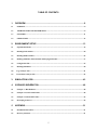
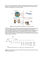
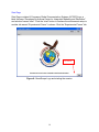
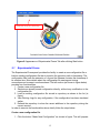
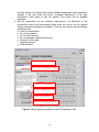
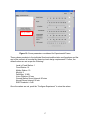
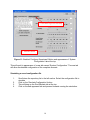
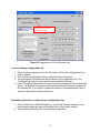
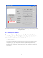
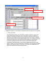
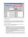
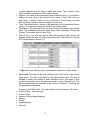
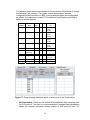
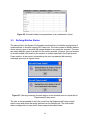
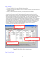
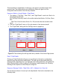
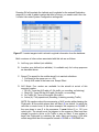
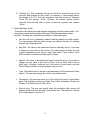
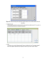
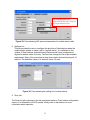
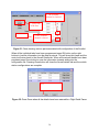
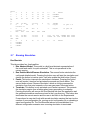
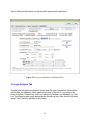
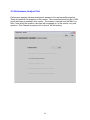
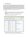
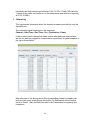
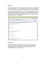
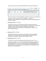
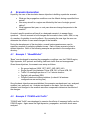
DEFENSE INFORMATION SYSTEMS AGENCY
JOINT INTEROPERABILITY TEST COMMAND
FORT HUACHUCA, ARIZONA
GenetScope - NetSim 2
Software User’s Manual
July 2006
DRAFT Version 1.1
GenetScope - NetSim 2
Software User’s Manual
July 2006
DRAFT Version 1.1
Prepared for :
Engineering, Analysis, Design and Development (EADD)
Engineering and Sustainment Support Task
HF Global Communications Systems (HFGCS)
United States Air Force
Tinker, Air Force Base
Prepared by :
Arizona Center for Integrated Modeling and Simulation (ACIMS)
Department of Electrical and Computer Engineering
University of Arizona
Prepared Under the Direction of:
Joint Interoperability Test Command
Fort Huachuca, Arizona
2
EXECUTIVE SUMMARY
The NetSim 2 is an object-oriented discrete-event system modeling and simulation
(M&S) environment to support simulation and analysis of voice and data communication
scenarios for High Frequency Global Communication Systems (HFGCS). The
application runs on Java™-based platforms, including both Windows and Linux and
allows a user to model a wide range of HFGCS communications and connectivity
operations through its own Graphic User Interfaces (GUI). NetSim 2 has been
developed not only to improve the implementation of original Automatic Link
Establishment (ALE) protocol in its predecessor, NetSim 1, but to provide the advanced
M&S framework, Discrete-Event System Specification (DEVS) for HF network models to
be reusable and scaleable systematically by adding more complex functionalities and
protocols throughout the future development cycle.
The earlier Netsim version (developed in 1997) was used to analyze any given scenario,
whether of past or in future based on ICEPAC prediction data. The current version aims
to take a quantum leap by providing the capabilities to not only analyze any scenario,
but provide recommendation to re-design the SCOPE command itself. The underlying
DEVS theoretical framework with its advanced features of real-time simulation
visualization and ability to configure simulation on-the-fly gives the analyst the power to
understand the impact of any design-parameter and how the system transitions to the
new parameter-set in real-time without restarting the simulation. This aids in changing
the corresponding parameter in the deployed SCOPE command system as the analyst
can study the transition effects. This capability to study transition effects by changing the
parameter set in real-simulation-time has been recently developed and is unique to the
DEVS framework. DEVS with its power of Experimental Frame helps focus the top-level
design issues like how many ground stations are best, how many internal levels are
minimally needed, what is the capacity of the system or what is the threshold SNR that
the system needs to continue to perform, optimally.
This User’s Manual gives the system overview of NetSim 2 environment and documents
the steps to setup and run experimentation of HFGCS network models. The example
communications scenarios are described for a user to run the system for exercise.
JAVA is registered trademark of Sun Microsystems, Inc. in the United States and other countries.
DEVSJAVA, Copyright 2002 Arizona Board of Regents on behalf of The University of Arizona
3
(This page intentionally left blank.)
4
TABLE OF CONTENTS
1.
OVERVIEW.............................................................................................................. 8
1.1
PURPOSE ......................................................................................................................................................8
1.2
ARCHITECTURE AND BACKGROUND.................................................................................................8
1.3
FEATURES .................................................................................................................................................11
1.4
LIMITATIONS ...........................................................................................................................................12
2.
ENVIRONMENT SETUP........................................................................................ 13
2.1
Experimental Frame ...................................................................................................................................15
2.2
Defining Fixed Stations ...............................................................................................................................20
2.3
Defining Mobiles Station.............................................................................................................................26
2.5
Defining Simulation Time Duration and Propagation model..................................................................37
2.6
Configuration File .......................................................................................................................................39
2.7
Running Simulation ....................................................................................................................................40
2.8
Logs Analysis Tab........................................................................................................................................41
2.9
Performance Analysis Tab..........................................................................................................................42
3.
SIMULATION LOGS.............................................................................................. 43
4.
SCENARIO GENERATION ................................................................................... 48
4.1
Example 1 “BaseWithAnt”........................................................................................................................48
4.2
Example 2 “CONUS with Traffic” ............................................................................................................48
4.3
Example 3 “Global with Traffic”...............................................................................................................49
4.4
Developing Scenario’s .................................................................................................................................49
5.
APPENDIX............................................................................................................. 51
5.1
Installation Instructions..............................................................................................................................51
5.2
Directory Structure. ....................................................................................................................................51
5
5.3
Bug reports with contact information .......................................................................................................52
Credits ....................................................................................................................................................................53
Copyright Notice.....................................................................................................................................................53
License Information ................................................................................................................................................53
Disclaimer...............................................................................................................................................................53
6
(This page intentionally left blank.)
7
1.
OVERVIEW
1.1
PURPOSE
The purpose of NetSim 2 is to provide a user-friendly discrete-event M&S environment
for a user to test the performance of the ALE system under various loads and
specifications.
1.2
ARCHITECTURE AND BACKGROUND
SCOPE Command is a highly automated, high-frequency (HF) communication system
that links US Air Force command and control (C2) functions with globally deployed
strategic and tactical airborne platforms. SCOPE Command replaces existing USAF
high-power HF stations with a communication system featuring operational ease of use,
dependability, and seamless end to end connectivity comparable to commercial
telephone services. The network consists of 15 worldwide HF stations (Figure 1)
interconnected through various military and commercial telecommunications media
(Figure 2). It increases overall operational and mission capabilities while reducing
operation and maintenance costs.
Figure 1: Geographic locations of Fixed stations
The HF radio equipments include Collin's Spectrum DSP Receiver/Exciter, Model RT2200. The radios feature Automatic Link Establishment (ALE) and Link Quality Analysis
(LQA) capability and are adaptable to future ECCM waveforms FSK, MIL-STD-188110B and STANAG 5066. The transmit subsystem includes 4-kW solid-state power
amplifiers, a high-power transmit matrix, and combination receive/multicoupler antenna
matrix. A typical SCOPE Command station includes operator consoles (HFNC), circuit
switching equipment (DES, DSN, LCO), HF radios (ALEs), RF matrixes (RTs), and
antennas (RXs, TXs). A non-blocking digital electronic switch (DES) connects the
8
station to the local military and/or commercial telecommunication services. The switch
features unlimited conferencing, modular sizing, digital switch network, precedence
function, and capacity for up to 2016 user lines.
Figure 2: Communication flow diagram for SCOPE command
SCOPE Command uses a modular, open-system design to automatically manage and
control all network operations, including those at split-site stations. To achieve
maximum flexibility, the system uses commercially available standards-based software
and a multitasking operating system. This approach permits 14 out of 15 network
stations to operate "lights out" (unmanned) and to be economically controlled from a
central location. The control system also includes LAN software, servers, and routers to
support unlimited LAN/WAN.
Figure 3: System Entity structure for SCOPE command system showing the fixed and
mobile (aircraft) stations
9
The program includes a Systems Integration Lab (SIL) and test-bed facility located in
Rockwell Collins' Texas facility. The SIL is used to predict the impact and risk that any
changes or upgrades will have on system performance, integrity or costs before actual
implementation begins. The SIL includes a fully functional SCOPE Command station for
performing baseline design verification, interface compatibility and functional verification
tests.
Joint Interoperability Test Command (JITC) is the only government agency that is
assigned the task to validate and authorize IT systems for military operations. The HF
SCOPE command system has also been evaluated by JITC. In collaboration with Dr.
Eric Johnson, a simulator was developed in the C language around 1997 that was
validated and eventually used by both the government and the industry to conduct
experiments and run scenarios. The simulator was an exhaustive and comprehensive
effort with respect to the details it implemented and served its purpose well. However, in
today’s circumstances, the same simulator is obsolete due to the heterogeneous nature
of today’s network traffic, in which E-mail occupies a considerable percentage of traffic.
The simulator is now being upgraded at the ACIMS lab in order to make it more useful
for current demands. These demands stem from the possibility of expansion of current
infrastructure of SCOPE command. Questions arise such as how many stations need
be added to service a required workload. Also needing to be investigated are tradeoffs
such as whether it is more economical to add more stations or increase the number of
internal radio-levels within stations to meet the anticipated demands. Air-traffic has
increased manifold since 1997, along with the computing technology. Consequently, the
transition effects need to be monitored more closely and the overall system response
time1 needs to be documented. The significant parameters have to be identified that
have the most impact on system performance. To more easily address such questions,
an effort is being made to modularize Johnson’s 15K lines of code into component
based structure depicted in Figure 3.. Once componentized, the components are made
DEVS compliant resulting in a DEVS-based simulation package to support the systems
engineering needs of the SCOPE command.2
As we need to study the effect of changes/upgrades introduced to the existing SCOPE
command system, we built the Experimental Frame, based on DEVS principles for our
modular DEVS-netsim simulation model, named as GENETSCOPE. Figure 4 shows the
block architecture of the simulation model. The right hand box is the system
phenomenon that contains the Automatic Link Establishment (ALE), STANAG 5066
protocols used for establishing links and exchanging data messages between mobile
stations and fixed stations. The left hand side box is the experimental frame that
generates various scenarios and parameters under study. The scenarios and
parameters are fed into the model and performance characteristics are obtained from it
which are then visualized and analyzed in real-time as per the extended MVC
architecture described in Section 5.
1
Response time of a system is defined as the time taken by the system to display significant effect
caused by any update in the configuration parameters.
2
A methodology using intermediate XML processing to automate much of the process of.
‘componentizing’ legacy simulation code will be reported soon
10
Figure 4: GENETSCOPE simulation architecture for SCOPE command
SCOPE Architecture implementation using enhanced Mode-View-Controller
paradigm
The Figure 5 below shows the simulation architecture using the concepts laid out in the
paper. With reference to Figure 4, the Ionosphere model used in the architecture is
ICEPAC data. It is worth stressing that initial Netsim model written in C language has
this database tightly coupled with the model. In our present implementation, we made it
modular so that it can be replaced by any other database that could provide the channel
propagation values through the ionosphere, for ex. VOACAP. The DEVS Layer
comprises both of model as well as the DEVS simulation environment. The
Experimental Frame layer contains the controls required to modify/update the model as
well as simulator as per enhanced MVC. The simulation visualization is modular in
construction and reflects the updates in Experimental Frame layer and the DEVS layer.
Figure 5: Simulation architecture for SCOPE command network
1.3
FEATURES
The GUI of NetSim 2 is arranged in a tabbed notebook fashion, separating each part of
the system into its own page. The major components are Fixed Sites, Mobiles (i.e.
11
aircraft), Frequencies that will be used for communication, and simulation parameters. A
fifth page provides a list of worldwide locations, which can be selected as needed for
placement of fixed communication sites or points as part of aircraft flight paths.
This version GenetScope 1.1 contains the Antenna configurations as shown below
Antenna
Number
1
Antenna
Type
LTO
GUI
sign
LTO
TX
RX
X
X
Samples\sample32
2
HTO
HTO
X
X
Samples\sample09
3
RLP
RLP
X
X
Samples\sample05
4
Rosette
ROS
X
X
Samples\sample32 (1)
5
6
Dipole
Vertical
Monopole
Whip
Probe
DIP
VTM
X
X
X
X
Samples\sample23
Samples\sample10
WHP
PRB
X
X
X
X
DEFAULT\SWWHIP.VOA
DEFAULT\SWWHIP.VOA(2)
7
8
Filename
Comment
(3)
Fixed
station
antenna
Fixed
station
antenna
Fixed
station
antenna
Fixed
station
antenna
Mobile
Mobile
Mobile
Mobile
(aircraft)
9
10
Other
X
X
User input
Notes
(1) Use LTO antenna until a better antenna can be found.
(2) Use Whip Antenna until a better antenna can be found.
Fixed station antennas should be selectable by any system. Fixed stations should offer
antennas 1-4 and 10 as selections.
1.4
LIMITATIONS
The NetSim 2 environment requires PC with a Pentium 4 or greater processor, with at
least 512 MB RAM. Recommended RAM is about 1GB. Depending on the details
required in log-files (especially EventLog), the minimum hard-disk capacity required for
an individual simulation run is between the ranges 20-1000MB.
GenetScope model limitations:
1.
The current model developed in Phase I of the project is bounded by the
functionality in the older Netsim version designed by Dr. Johnson in C++. It
has been translated and developed using the DEVS theory and implemented
in Java. No new ALE functionality has been added in the current version.
12
2.
3.
4.
2.
All the stations in any scenario work on default AFALE scanlist. However,
provisions to program different scanlist have been added into the
configuration GUI. The associated functionality will be implemented in the
next version-build of GenetScope, possibly in Phase II of the project.
The model is in developmental Beta stage and validation of simulation results
with real-time JITC data is undergoing. Error reporting is highly
recommended.
No terrestrial networks have been introduced in the current version. They are
left for Phase III of the project.
ENVIRONMENT SETUP
About
Clicking the About button will present the related information, version and involved
personnel associated with this project.
Help
Clicking the Help button will open the pdf version of this document Manual in Internet
Explorer window.
13
Start Page
Start Page contains Hi Frequency Global Communication Systems (HFGCS) logo, a
label that says “Developed by Arizona Center for Integrative Modeling and Simulation”,
and a button named “start”. Push the “start” button to continue the environment setup or
another tab named “Experimental Frame” is shown. Click the “Experimental Frame” tab.
click here
Figure 6: GenetScope Logo and starting the session
14
click here to go to a next step
Figure 8: Appearance of Experimental Frame Tab after clicking Start button
2.1
Experimental Frame
The Experimental Frame panel provides the facility to create a new configuration file or
load an existing configuration file that is stored in the repository with its timestamp. The
configuration files have the extension of .cfg and the filename contains the timestamp of
its creation time. More details about the configuration file naming and storing
conventions can be seen in sections ahead. The left section (as shown in figure below)
provides four functionalities:
1. Create a new configuration file
2. Simulate an already saved configuration directly, without any modification to the
configuration file
3. Load an existing configuration file stored in repository as shown in the list (in
figure)
4. View Existing Logs for any configuration, if the configuration has been simulated
earlier.
5. Refresh the repository to show the recent additions in the repository during the
current session.
In order to execute the functionalities above kindly follow the steps below:
Create a new configuration file
1. Click the button “Make New Configuration” as shown in figure. This will prepare
15
the right section of the pane and load the default experimental frame parameter
settings. It will also make the button “Configure Experiment” in the right
bottommost (scroll down to see the button). This button will be disabled
otherwise.
2. Set the parameters as per scenario requirements. As described in the
architecture section the Experimental frame gives the user to set the general
design parameters guiding any scenario. The user can specify top-level design
parameters like:
a. Level in a fixed station
b. No. of fixed stations
c. No. of mobile stations
d. No. of messages transmitted per hour
e. Duration of voice calls
f. Sounding interval
g. SNR threshold
To a new configuration file
Show saved Configuration files
Simulate Configuration
Load a configuration file
View Existing Logs
Refresh configuration files
Figure 9: Basic operations related to saved Configuration files
16
Set up values
Figure 10: Some parameters considered for Experimental Frame
These values percolate to the individual fixed and mobile station configurations and the
rest of the scenario is bounded by these top-level design requirements. Further, the
default values are set as per the following::
Level in Fixed Station: 1
Fixed Station: 14
Mobile Station: 10
Msg/Hr: 2
Data Msg: 10 KB
Voice Duration: 60 sec
Ground Station Sound Interval: 90 mins
Aircraft Sound Interval: 90 min
SNR Threshold: -6 dB
Once the values are set, push the “Configure Experiment” to store the values.
17
2. click here to go to a next step
1. Push the button
Figure 11: Enabled ‘Configure Experiment’ Button and appearance of ‘System
Configuration’ tab at the top
This will result in appearance of a new tab named ‘System Configuration’. The new tab
will allow the detailed configuration of the complete scenario.
Simulating a saved configuration file
1.
2.
3.
4.
Scroll down the repository list in the left section. Select the configuration file to
simulate
Click on the ‘Simulate Configuration’ button.
This will bring up the Run/Simulate tab at the top.
Click on the new appeared tab and proceed towards running the simulation.
18
Select the tab to the
Simulation pane
Figure 12: Appearance of ‘Run/Simulate’ tab
Load an existing configuration file
1. Scroll down the repository list in the left section. Select the configuration file to
load or update.
2. Click on the “Load/Update” button in the left section of the pane
3. The right section will reflect the stored values in the configuration file. The
“Configure Experiment” button will also get enabled at this point.
4. Press “Configure Experiment” to move to System configuration tab as described
above. The System Configuration will load the existing information contained in
the selected file. If you need to update the values for the experimental frame, it
should be done before clicking this button.
Refreshing Repository to show stored configuration files
1. Click on the button “Refresh Repository” to view the updated repository if you
have saved/created any new configuration files in the current session.
2. The list above will reflect the current status of repository.
19
1. Push the button
Figure 13: Refresh Button to refresh the contents of Repository to view recently created
configuration files
2.2
Defining Fixed Stations
The main page of System configuration begins with a “Fixed Station” tab. The tab
consists of four parts such as the list of stations, station info panel, station info tabbed
pane, and modification of stations data. Before starting this panel, the data structure of
stations should be created and the values should be set.
1. The list of stations
The number of fixed stations is obtained from the previous step. Default number of
“fixed station” is 14. The stations with “Checked” checkboxes are active in the
simulation while “Unchecked” stations are inactive. User can check or uncheck the
fixed stations.
20
2. Station info panel
3. Modify stations data
4. Station info tabbed pane
1. The list of stations
Figure 14: Snapshot of Fixed Station configuration Pane showing various sub-panels
2. Station info panel
This panel displays station call, ALE Activity, Latitude, Longitude, Location, and
lookup. Station call is entered by a user. If any station on the list of stations is
checked or unchecked, the station call of the station is displayed on the text field.
ALE Activity is a combo box that contains the two values, i.e., “Active” or “Passive”.
Latitude, Longitude, and Location can be typed by a user. The “Lookup” button sets
all the fields of station info panel and station info tabbed pane with all station
information regarding the station call. In order to view the information and
configuration of any fixed station, enter the three alphabet call-sing of the fixed
station in ‘Station Call’ text field and press Lookup button. This will show the details
related to that particular station. All the tabs in the ‘Station Info tabbed pane’ will
reflect the information associated with that station.
21
After click the “Lookup” button
Figure 15: Showing the related info about a fixed station when Lookup is pressed
3. Modify stations data
If some changes are to be made by a user, the station data can be updated by
clicking the “update” button. The user can delete any station using a “delete” button.
Users can make stations and save information of stations using a “add” button.
4. Station info tabbed pane
This pane is composed of five tabs named “Message Traffic”, “Ale Levels”, “Ale
Parameters”, “Scan List”, and “Gnd InfraStructure”
•
•
•
Message Traffic: This tab allows for setting up the traffic stream parameters
originating from this fixed station. It will take the default values as set under
the Experimental Frame section but user can override the internal details of
the traffic stream. Each row is a single traffic stream. The user can program
more than one traffic streams origination from the station. The details of any
single traffic stream can be programmed as under:
Use: the first row is checked by default reflecting atleast one traffic stream.
You can program different traffic streams and uncheck the box for updating
any existing configuration file.
Msg Size: The value in the experiment frame is internally set up. If you want
to change, put any value in the text box. The value entered is either seconds
22
•
•
•
•
or bytes depending on the value of traffic type under “Type” column. Voice
traffic is taken in seconds and Data traffic in bytes.
Msgs/hr: The value in the experiment frame is internally set up. If you want to
change, put any value in the text box.Type: Voice or Data. With Voice as
traffic type, it implies 2 calls per hour (as shown in figure below) and with
Data it reflects number of data messages sent per hour.
Type: The default value is shown as programmed in the Experimental Frame
section. The user can change this value on per station basis.
Precedence: The user can select any of the five priority levels on per station
basis. The available priorities are Flash Over, Flash, Immediate, Priority and
Routine. The default value is Flash Over.
Start at (min): The user can specify when this particular traffic stream will
become operational from the start of simulation time. This feature is currently
NOT implemented in Version 1.0.
Figure 16: Pane showing various parameters needed for a traffic stream
•
•
•
•
•
•
•
•
Ale Levels: This tab will allow for configuring the ALE levels in the chosen
fixed station. The value is bounded by the Experimental frame. The user is
allowed to specify the details of each individual level in this pane. It also
provides information about the antennas used at each individual level. The
antenna parameters are defaulted in this version of Netsim-2. Following are
the parameters considered:
Number of ALE Radio Sets : the total number of levels(maximum 16 levels)
Power (Watts) : antenna power
Antenna Type
Antenna Pointing Angle(degrees)
Mission
Priority
Angle(degrees)
Gain(db)
23
The columns empty below are intended for future version of the Netsim-2 except
the Antenna Type columns. The current version does support antenna
configurations and its effects on SNR. Various antenna types can be described
as follows. If no selection is made LTO is default in Fixed stations and Whip is
default in mobile stations.
Antenna
Number
1
Antenna
Type
LTO
GUI
sign
LTO
TX
RX
X
X
2
HTO
HTO
X
X
3
RLP
RLP
X
X
4
Rosette
ROS
X
X
5
6
DIP
VTM
X
X
X
X
7
8
Dipole
Vertical
Monopole
Whip
Probe
WHP
PRB
X
X
X
X
9
10
Other
X
X
Comment
(3)
Fixed
station
antenna
Fixed
station
antenna
Fixed
station
antenna
Fixed
station
antenna
Mobile
Mobile
Mobile
Mobile
(aircraft)
Figure 17: Pane showing individual details of every level in the Fixed station
•
Ale Parameters: These are the default ALE parameters that are being used
for ALE protocol. The user is not recommended to change these parameters
unless the scenario demands studies related to ALE protocol itself. For
24
convenience purposes, these values can NOT be changed in the current
version. The only programmable value here is Sounding Interval, which is
specified in the Experimental Frame and is reflected here.
Figure 18: figure showing default ALE protocol parameters
•
Scan List: This tab provides the user to select any available Scan list. A
Scan list is defined as a set of frequencies being used by that particular
station to communicate with other stations. The defaulted choice is AFALE
Scan list. There are four Scan list supported by Netsim-2. Each Scan list has
unique channel list independent of other types and each channel internally
translates to a single frequency. If one of the radio boxes is clicked, then text
area displays the channel list of the radio box. ALE Freq table shows the
channel, frequencies of each channel, and check boxes that mean if
checked, the channel in the first row is used and if not, the channel is
available. The channel used by a type can not be selected by other types.
Figure 19: Figure showing scanlist operations at the station.
•
Gnd Infrastructure: This panel is left for further development in the near
future.
25
Figure 20: Ground infrastructure parameters to be considered in future
2.3
Defining Mobiles Station
The second tab in the System Configuration section allows for detailed configuration of
mobile stations or aircrafts carrying ALE radio sets. The main screen for Mobile stations
shows various types of aircrafts that can participate in any particular scenario. The user
can select different types of aircrafts for the current scenario. However, the total number
of aircrafts added is bounded by the number of mobiles specified in the Experimental
Frame section. In the event of mismatching the user is presented with warning
messages as shown in figures below.
Figure 21: Warning message if mobile station count selected does not equal that of
Experimental Frame count
The user is recommended to verify the count from the Experimental Frame mobile
station count and select that many stations from the Mobiles tab. The total mobile
station configuration is executed in three steps as described below:
26
Step 1: Mobiles
1. Choose “Mobiles” tab to open Mobiles station setting
2. Choose the combo box which is next to the name of aircraft, and then select the
number of aircraft.
3. After you have finished the selection, push the button “Enter Details”.
In order to aid the user to verify if he has selected the correct number of mobile
planes, the pane above shows both the Experimental Frame value and the number
that the user has selected in above combo boxes. The user can go to the next process
only when these two numbers exactly match. One word of caution in the current
version is that the user has to look into the flight details more closely, if he is updating
an already saved configuration file. There exists no problem if the user is increasing
the mobile station count, but if he chooses to diminish the mobile station count, he is
recommended to verify the flight details and update too as a part of configuration
process. The ability to delete any selected mobile station from an existing
configuration file will be added in the next Build.
1. The selected Aircraft is “C5”, and
the number of “C5” is “one”
3. If all the numbers of aircraft has been selected, n push
“Enter Details”
2. The selected Aircraft is “C130”, and
the number of “C130” is “two”
Figure 22: Main Mobile Station selection pane
Step 2: Aircraft Details
27
This step allows for specification of call signs to the types of aircrafts chosen in the
previous step. The mobile stations are identified by these call signs for all the
configuration and simulation from this step onwards.
Sequence: Mobile > Aircraft Details > Flight Detail
1. The values of “Call Sign”, “Start Time”, and “Flight Details” need to be filled in for
the selected aircraft type.
Ex) Call Sign: Enter any name for the mobile station identification. Ex) Sam, Steve,
Bon
Start Time: Enter the take off time. Ex: 120 (minutes after the simulation start
time).
2. Click the “Flight Detail” button to fill out the details of the selected aircraft.
3. The “Flight Detail” dialog with the Call Sign name is popped up.
1. Fill out the name of
“Call Sign”
2. Fill out the
start time.
3. Push the “Flight
Detail Button”
Figure 23: Pane showing the call-sign and start up details of the chosen flight planes
Step 3: Flight Details
Clicking on Flight Details tab will pop up a new dialog box that aids in configuration
specifics about this particular mobile station. The user can provide details about the
message traffic originating from it, its flight path, ALE radio parameters, the address list
that is the prioritized in order of calling to fixed stations, and frequency lists. Showing
following is the sequence in which they are configured.
Sequence: Message Traffic > Flight Path > ALE > Address List > Scan List
The five tabs are shown to be set up for the flight details. Each tab is described in the
following steps.
28
1. Flight Path
This tab provides the functionality to program the flight path of any particular
mobile station. The user is required to double-click in the Locations column.
Figure 24: Pane showing the Flight Path planning configuration
This will enable the text area in that cell. Kindly enter one or two words descriptive
of the location serving as waypoint (shown in the left figure below). Press tab-key
or Enter to search with this location name and press Lookup Location button.
Pressing the lookup button will popup the locations that contain that particular
word. In the right figure below, all the location containing the word “Dover” (from
the left figure) are listed (as they exist in the locations database). Select the exact
location and press Ok.
Figure 25: Put any keyword related to
the desired waypoint and press either
Tab or Enter
29
Figure 26: Pressing Lookup shows
all places containing the keyword in
left figure
Pressing OK will populate the Latitude and Longitude for the entered Destination
waypoint. In order to add a location that fails to lookup, you need to add it thru the
‘Location’ tab under System Configuration settings tab.
Figure 27: Loaded waypoint with Latitude Longitude information from the database
Brief overviews of other values associated with this tab are as follows:
A. Lat/Long: pre- defined (not-editable)
B. Location: pre- defined (not-editable). It is editable only for Lookup purposes
as described above.
C. Speed: The speed for the mobile aircraft is in nautical miles/hour
i. Put Speed in the upper row. ex. 450
ii. Set up ALE mode in the lower row. Except Silent
D. ALE Mode: Four modes are available for the aircraft at arrival of this
waypoint location.
i. Off (O): Turns the ALE radio off. (No traffic, no sounding, no listening)
ii. Silent (S): Turns ON the ALE radio (No traffic, no sounding)
iii. No Traffic (N): Turns off the traffic (No traffic)
iv. Active (A): Fully operational (Sounding, Listening, sending Traffic)
NOTE: Be cautious about the sequencing of ALE modes while planning the
Flight-path. All the mobile planes start as Silent (S) as default, on which the
user has no control over. In the above example, the sequence is: SAAAS. If
the user plans to use O in the sequence, S must follow O i.e. OS is an
orderly pair. The aircraft must first appear on the scene as Silent and then
change its mode to Active or No Traffic or stay as Silent. If user wishes to
begin the Flight-path by switching the radio silent and turning it ON after
certain waypoints then the sequence formed is SOSAS or SOOSANS etc.
30
E. Duration (hr): This represents the time at which the aircraft arrives at this
waypoint and changes its ALE mode. For example, in the example above,
the aircraft at 0.15 hr from the simulation start time arrives at Waypoint
Dover DE and become ‘Active’. Similarly, the aircraft reaches second
waypoint Falmouth ME after 2 hours of previous waypoint and remains
‘Active’.
2. Mobile Message Traffic
This section tab defines the traffic streams originating from this mobile station. The
description is same as fixed station Message Traffic tab described in earlier
sections. For ease, the configuration procedure in delineated again.
•
Use: the first row is checked by default reflecting atleast one traffic stream.
You can program different traffic streams and uncheck the box for updating
any existing configuration file.
•
Msg Size: The value in the experiment frame is internally set up. If you want
to change, put any value in the text box. The value entered is either seconds
or bytes depending on the value of traffic type under “Type” column. Voice
traffic is taken in seconds and Data traffic in bytes.
•
Msgs/hr: The value in the experiment frame is internally set up. If you want to
change, put any value in the text box.Type: Voice or Data. With Voice as
traffic type, it implies 2 calls per hour (as shown in figure below) and with
Data it reflects number of data messages sent per hour.
•
Type: The default value is shown as programmed in the Experimental Frame
section. The user can change this value on per station basis.
•
Precedence: The user can select any of the five priority levels on per station
basis. The available priorities are Flash Over, Flash, Immediate, Priority and
Routine. The default value is Flash Over.
•
Start at (min): The user can specify when this particular traffic stream will
become operational from the start of simulation time. This feature is currently
NOT implemented in Version 1.0.
31
Figure 28: Pane showing the originating Traffic streams from mobile station with call
sign Sam
3. Mobile Levels
The user can specify the antenna that is onboard the mobile aircraft. If no option is
selected Whip antenna is selected by default.
4. ALE
The value set up in the Experimental Frame is reflected in the “Sounding interval”
field in the panel. Others are not required to be set up in the current version.
32
The Sounding interval is
reflected from the value setup in
the Experimental Frame
Figure 29: Pane showing ALE protocol parameters for mobile station radio
5. Address List
This tab provides the user to configure the priorities of fixed stations when the
mobile station wishes to make a call to ‘ground station’. It is defaulted to the
number of fixed stations (selected during Experimental Frame configuration)
aligned in random order of priority. The user can change this list as per scenario
requirement. Each of the row below is drop down combo box each having all 14
stations. The defaulted value is 14 stations, hence 14 rows.
Figure 30: Pane showing the calling list of mobile station
6. Scan List
The Scan list tab is identical to the tab mentioned earlier in Fixed station configuration
section. It is defaulted to AFALE scanlist. Kindly refer to that section for more
information about operation
33
3. The available
channel is checked.
1. Select one
of the lists
2. The available
channel is shown
Figure 31: Pane showing various parts associated with configuration of the Scanlist
When all the individual tabs have been programmed press OK button on the right
bottom to load the information into the data structures. This will close this frame and the
control will return back to the Aircraft Details tab. When all the aircraft details have been
populated press Done button to save the information towards writing into the
configuration file. Pressing Done button will close the Aircraft details tab and the mobile
station configurations are complete.
1. Press Done to save all the aircraft
details.
Figure 32: Press Done when all the details have been entered thru Flight Detail Panes
34
2.4
Defining Channels and Locations
Frequency/Channel database
The frequencies available in the system are shown. User can choose the Scan list in the
Comments combo box. There are currently 100 channels defined that correspond to
100 frequencies. Various other constraints like power on which they operate, restricted
access and their categorization are also provided here. This is the master channel table
and each channel is configured to lie in atmost one scanlist. The mapping is provided in
Comments section where the user can specify whether the channel belongs to either of
the following:
1. NIPRNET
2. SIPRNET
3. CAPNET
4. Published
5. Discrete
6. Not in use
Figure 33: Master Channel-Frequency table and their classification in various Scanlists
Locations
This top-level tab shows the location database used by the model. The geographical
locations specified here can be used to program the flight path of any mobile station.
The user can add, delete any location and it is saved in the local database for future
35
use. A location once deleted can not be retrieved back; the location data is shown in the
table. The basic operations on the list are performed as under:
A. Add
i.
Click the lower row you want to add.
ii.
Push Add button.
iii.
Once the empty row will be shown, put the value in the each box.
B. Delete
i.
Select the row you want to delete
ii.
Push Delete button
C. Save
Once you edited all value, push the Save button.(It will take for a while)
If you push “add” button,
the new row is created in
the just upper row you
select
Figure 34: Pane showing the complete Location database with functionality of
adding/removing/updating any location
36
2.5
Defining Simulation Time Duration and Propagation model
Once the Fixed stations, Mobile stations, master Channel list, Locations database are
set, the scenario generation is almost complete. The only thing remaining now is to
specify the time and duration of simulation. This can be specified from the ‘Setup’ tab
shown below. The simulation start time is specified in 24 hour notation. The duration is
determined by specifying the End time of the simulation in 24 hour notation. The GUI
identifies the operational Sun Spot Number (SSN) based on the year-month-day. The
identified SSN is then used to gather ionospheric propagation data. The user can either
choose ICEPAC or VOACAP. In case of no selection, ICEPAC is chosen as default.
The analyst can enter any descriptive text concerning this simulation configuration.
Figure 35: Simulation setup tab for the scenario loaded/configured
37
Once the time-date are configured, pressing the ‘Write files’ button will result in a
configuration file in .cfg format saved in hard-disk (opened thru Wordpad application). In
addition to writing up the configuration file, the configuration is also loaded to the
simulation model to enable the simulation with current configured scenario. Information
will pop up displaying that the configuration is now complete, validated according to the
Experimental Frame settings and stored at what particular location.
Figure 36: Error messages if the user enters a month or year not supported by the
Model
Figure 37: Confirmation message notifying that configuration is complete, stored and
ready to be simulated
Clicking on the Write Files button will add the Run/Simulate tab at the top level indicated
in the figure below. At this juncture, the scenario is completely configured, saved in a
dedicated folder for this simulation run and ready for simulation.
38
2.6
Configuration File
The process described in previous section results in saving a configuration file identified
by its timestamp as suffix and is saved in the application’s ‘Configuration’ folder. The
file’s name is automatically configured based on the timestamp, e.g.,
config4.4.12.21.05.cfg where the numbers translate to 4:04am on 12/21/05. The sample
shown below consists of 2 Fixed stations and 1 mobile station. Others description
details are not required as per the current document.
E
1
6
1
2
60
V
90
60
-20
S
16:00:00
1:00:00
3
33
V
#
@
Enter descriptive text to provide information about the scenario
# with SSN = 33
#
#
F MCC 38.650
-121.383
-114 A
WestCoast
ALE
RT
PA
ANT
ASP
Bcast
C
C
C
C
#D
F HIK
1
1
1
1
VTM
2
3
1
90
4
6
5
91
21.317
ALE
RT
PA
ANT
ASP
Bcast
C
C
C
C
#D
F OFF
41.267
ALE
RT
PA
ANT
ASP
1
1
1
1
LTO
8
9
7
92
10
12
13
93
11
16
15
94
14
21
18
95
17
22
20
96
19
AFALE
NIPRNET
SIPRNET
97
CAPNET
-157.867
-114
A
Hickam
8
9
7
92
11
16
15
94
14
21
18
95
17
22
20
96
-114
A
Offutt
1
1
1
1
ROS
2
3
1
90
4
6
5
91
10
12
13
93
-95.950
39
19
AFALE
NIPRNET
SIPRNET
97
CAPNET
Bcast
C
C
C
C
#D
#
M
T
T
L
2
3
1
90
4
6
5
91
8
9
7
92
150
35.466
0
3
60
minutes ea
0
1
20
minutes ea
MCC
HIK
OFF
10
12
13
93
11
16
15
94
-97.533
10
V
250
D
AED
JNR
W
W
ASP
C
C
C
C
#D
0.1
35.466
4.0
39.166
WHP
2
4
8
NIPRNET
SIPRNET
CAPNET
2.7
Running Simulation
14
21
18
95
17
22
20
96
19
AFALE
NIPRNET
SIPRNET
97
CAPNET
S
C5
~3
455684
msg/hr
to gnd ~1.0
~1
msg/hr
to gnd ~20
ADW
-97.533
-75.533
A
S
CITY OK USA TINKER AFB
DOVER DE USA DOVER AFB
10
14
17
11
19
USAF
USAF
AFALE
Run/Simulate
This tab provides four functionalities
1. Run Abstract Model: This model is a high level abstract representation of
the model and useful for quick estimation. This is not operational in the
current version.
2. Run Detailed Model/Resume Simulation: The second button simulates the
configured detailed model. Pressing the button once will start the simulation and
change the button to inactive state. It will also enable the third button (Pause).
3. Pause: This button interrupts the simulation in between. Pressing this button
once will render it inactive and activates the second and fourth button. The
second button shows ‘Resume Simulation’ which on clicking resumes the
simulation from that point onwards or the user can press Terminate button.
4. Terminate: This button is only activated once Pause is pressed. This protects
the simulation engine from crashing when heavy processing is underway.
Pressing this button will remove the Run/Simulate tab from the application and
the gathered simulation results are stored in the Logs directory. This button also
terminates the current session and the user is led back to the Experimental
Frame where he can start fresh with second simulation session that can involve
creation of new configuration file, running an old configuration file or reloading a
saved configuration file. The Run/Simulate tab can be re-established for a
different configuration scenario once a running simulation is terminated.
40
Various fields and information on the simulation pane is self-explanatory.
Figure 38: Real-time Simulation Visualization Pane
2.8 Logs Analysis Tab
This particular tab gets activated and shown when the user ‘terminates’ the simulation.
Various logs are displayed. More details are provide in Section 3. Log Analysis tab
shows 6 log files, Channel log, ALE Log, Linking Log, Models Log, Message Log, LQA
Log. The internal engine reads and parses the textual log files, then shows in the table
format. “Print” button is disabled in this version.
41
2.9 Performance Analysis Tab
Performance analysis tab was developed to answer to the user’s possible question.
There are tentative five questions in this version. The conversion textual log file to XML
log file has been processed in this version. The answer is derived from the XML Log
files. If user clicks the question, the chart will be popped up. In this version, only one
question “ Give Channel occupancy list for hour x” will be working.
42
3.
SIMULATION LOGS
Once the simulation is termainated, it displays the logs and performance results in two
new tabs i.e. ‘Logs Analysis’ and “Performance Analysis’ tab. The simulation results in
generation of log files stored in the application’s ‘LOGS/configFile/’ folder as .txt files. All
the logs can be exported to Microsoft Exel for better analysis. Logs are tab delimited.
The log file names are automatedly time stamped in the same manner as the scenario
configuration file where the numbers have their usual meaning. If the configuration file is
named base223.0.3.10.06.cfg, the six log files are stored in “Logs/base223.0.3.10.06/”
folder and are displayed in the GUI in Logs Analysis tab as follows:
1. AleLog
This is the ALE radio log file and it shows which ALE radios are in which state
during the course of simulation run. The columns provide information in this
sequence:
StationID--Level—AtTime—OnChannel—toDestination—Status
A typical snapshot of this log file is shown below:
As can be seen above station 150 calls on channel 6 to station 1 at
01:06::02.400 s. It engages in linking procedure and gets linked after 3-way
43
handshake and both stations get linked at 01:06:13.190 s. Finally 150 starts the
1 minute Voice traffic and comes out of the linked phase and returns to scanning
at 01:07:19.388 s.
2. ChannelLog
This log provides information about the channel occupancy and activity over the
simulation run.
The columns provide information in this sequence:
Channel—Start Time—End Time—Src—Destination—Power
It tells us about which channel has been used at what particular time and who
are the two stations engaged in communication procedures. A typical snapshot of
this log is shown below:
With reference to the AleLog above the corresponding channel occupancy can
be looked into more detail through this logfile. 0 in Destination column implies
that it is ‘Sound’. Start and End time refer to the Transmission’s beginning and
completion.
44
3. LQALog
This particular log file is of most interest to the simulation run. It reports the LQA
scores by all the station on an hourly basis as the transmission are heard at its
end. The value shown in the table is the representation of Signal to Noise ration
heard at that station during that hour. It is in a table format where the receiver
station constructs a table with Channels on x-axis and heard stations on y-axis.
The following image shows the LQA table for ALE 170 that resides at Station
MCC and ALE 152 that resides as Station ADW, at level 1 in a given scenario
configuration at hour 1 of simulation run.
4. LinkingLog
This log provides information about the links that were established over
the course of simulation. The figure below is self-explanatory, with Qual
reflecting the LQA score (quality) and Time taken the duration for ALE
link establishment procedure execution.
45
5. MobilesLog
This log provides the information related to the flight path traversed by any mobil
e plane with the time-stamp. The log can be sorted based on
column CallSign to plot the trajectories of any specific mobile plane.
6. MsgLog.base223.0.3.10.06.txt
This log provides information about any messages that were attempted.
They are reported in this log if the station fails to deliver the message
(after repeated attempts too). However, it doesn’t show the retries. Only
the final outcome is reported with the reason of failure. If the message is delivere
d then it is reported too. Check the first message at 42:12.793 in
46
the figure below mirroring the link established thru AleLog and LinkingLog.
Some of the reasons if the message fails to deliver is absence of channel after re
peated tries. This is reported as “NO_CHANNEL”. In the above
snapshot, all the messages are reported delivered with their message type as eit
her Voice or Data.
7. PropLog.base223.0.3.10.06.txt
The purpose of this log is to document the ICEPAC software access and
Verify the returned values from ITSH software as and when they are used in the
simulation model. This is for exhaustive analysis of the simulation
analysis in conjunction with above logs. The details are not meant for the
user and hence omitted.
8. Errog.base223.0.3.10.06.txt
This particular log focuses on the errors that might be reported during the
simulation run. This log is entirely for development purposes and for any
feedbacks that designers might want the developers to know.
9. Eventog.base223.0.3.10.06.txt
This log is also meant for debugging and development purposes. It is not
required in production runs. It is recommended that this log be not generated
during the production runs as it is a huge log amount to few gigabytes for a
typical simulation run. It accounts for ever single event that is generated and
processed as the simulation proceeds forward. Again for clarity purposes, the
details are not provided herein.
47
4.
Scenario Generation
Hopefully, the user of the simulation has an objective in building a particular scenario.
•
•
•
What are the propagation conditions over the Atlantic during a specified time
period?
How many aircraft in a region are affected by the loss of a single ground
station?
What happened last year, or next year when we change frequencies in the
scanlist?
As noted, specific questions will result in a designed scenario’s to answer those
questions. Once a scenario is built changes can be made to time, traffic, SSN, or any
of a number of variables to see the effects. By comparing the user logs the user can
determine the effects of even small changes to the scenario.
During the development of the simulation, several basic scenarios were used to
examine a number of particular validation issues. Each of these scenarios’s had a
defined objective. Each of the following examples are provided in the configuration
directory.
4.1
Example 1 “BaseWithAnt”
“Base” was developed to examine the propagation conditions over the CONUS region,
flight dynamics, ALE protocol and linking, and basic traffic flow and management.
Given those objectives, the scenario was setup as follows:
•
•
•
•
•
Six ground stations (ADW, OFF, MCC, JNR, AED, HIK)
Single Aircraft flying between Tinker AFB, OK, to Dover AFB, DE.
Traffic 2-3 messages per hour of 1 to 5 minute duration
Daylight, with predicted SSN
Different Antenna at different stations (to check if all antenna
configurations are working fine).
Once the basic objectives were established, the scenario was developed, ran, analyzed,
modified, ran, analyzed, etc. Analysis was based on the basic, first run and data
obtained, and changes in the scenario were then compared to determine the effects of
the changes.
4.2
Example 2 “CONUS with Traffic”
“CONUS with Traffic” was developed to examine the effects of increased traffic over the
CONUS region. Again areas like flight dynamics, propagation, and traffic levels were
analyzed.
48
•
•
•
•
All ground stations (14)
Multiple Aircraft flying between locations CONUS.
Traffic 2-3 messages per hour of 1 to 5 minute duration
Daylight, with predicted SSN
Again like the “Base” scenario a baseline was established and changes were compared
to the basic data.
Changes to a particular scenario should be limited to only one or two of the variables,
with multiple changes it would be hard to determine what changes affected the output or
result of the scenario. By making multiple runs of the scenario with defined changes in
the scenario the cause and effect of the changes can be more readily determined.
4.3
Example 3 “Global with Traffic”
“Global with Traffic” was developed to examine the network with aircraft and traffic
dispersed around the globe. The differences in propagation around the globe, the
ability of the network as a whole to support world wide traffic and effects of aircraft
transiting between different coverage areas.
•
•
•
•
All ground stations (14)
Multiple Aircraft flying between locations world wide
Traffic 2-3 messages per hour of 1 to 5 minute duration
Start 16 GMT, with predicted SSN
Like the previous examples, specific objectives were established and the results were
analyzed.
4.4
Developing Scenario’s
In planning to develop a scenario, the user may expand on one of the example
scenarios or develop a new scenario with their specific objectives in mind. One thing to
remember is that the GenetScope/NETSIM 2 model, simulates each radio specified in
the scenario, sounding, traffic, the number of aircraft each add detail and thus the
complexity of the simulation. As such a very detailed scenario may take several/many
hours to run. So practicality dictates the best practices in designing and developing a
scenario.
The opposite also applies; to short of a scenario may not provide any or enough detail
to answer the questions posed by the user. The simulation models the real-world, in
both propagation, and ALE functionality. The JITC can provide assistance in
developing scenarios or analyzing the results of a scenario. One additional point to
remember is that the log files used for analysis are named after the scenario, so if you
49
modify the scenario but save it with the same name, the files will be written over. It is
suggested that log files be moved to an archive directory.
The Configuration files may be renamed to be more descriptive and it is recommended
that the comment field on the setup screen be used to define the scenario and any
objectives. These comments are saved with the configuration files.
50
5.
Appendix
5.1
Installation Instructions
1.
2.
Execute the GenetScope2.exe file by double-clicking it.
Specify a root folder for the files to get copied or the default folder will be
C:\ProgramFiles\ACIMS\GenetScope-Netsim2
Click Start->Programs->ACIMS->GenetScope-Netsim2
OR GenetScope2 icon on the Desktop to start the application.
3.
5.2
Directory Structure.
The application is tightly integrated with the directory structure below. The user is very
strongly recommended to not change the structure of this directory. Failure to do so
might deem the application not executable. The project directory contains the following
subdirectories/files:
1.
2.
3.
4.
5.
6.
7.
8.
Readme
GS1.0W.exe: Main application
GS1.0
This folder contains basic application Config files
GenetScope-Netsim2_Manual.pdf: Software User’s manual
Configuration
This folder all the generate or saved configuration scenario files with
extension .cfg. The files can be opened in Wordpad for viewing and manual
edition. However, it is not recommended to manually edit the Config files.
Three basic configuration files are available as described in the previous
section. The user can build on these files for reference.
a. Sample Archives
This directory contains the original three base files that must not be
changed. They are to be left as originals in case the user changes them in
the parent folder. The files stored in this sub-folder will not be visible in the
application GUI.
inst_files
This folder contains the required setup files for GenetScope application. None
of the files should be changed.
itshfbc
This folder contains the files required to run the ITSH propagation software for
dynamic SNR values required by GenetScope application. None of the files in
the directory should be changed.
Logs
This folder contains the simulation logs for production runs. If the user wishes
to run the simulation again for the same configuration file, it is very strongly
recommended that the user save the simulation logs of the previous run as
they will get overwritten. The Logs folder contains various sub-folders with the
name of the Configuration file. For example, if the configuration file name is
51
‘BaseWithAnt.cfg”, the Logs folder will contain a folder called “BaseWithAnt”
that will contain all the logs described earlier.
5.3
Bug reports with contact information
The GenetScope version 1.0.14 is in Beta status. Problems like locked-in might occur in
which the simulation clock stops before the end of simulation time. In the event of such
occurrence, the analyst is request to run the simulation again in “Debug” mode and
send the log files to the ACIMS development center. The log files along with usual log
files that must be mailed are:
1.
2.
3.
4.
EventLog
ExceptionLog
ErrorLog
Prop Log
The Email addresses are as follows:
Saurabh Mittal
Lead Developer
[email protected]
Seahoon Cheon
Team Member
[email protected]
Chungman Seo
Team Member
[email protected]
All the personnel above work at:
Arizona Center of Integrative Modeling and Simulation
Rm 318, ECE Department, University of Arizona,
Tucson 85721, AZ
www.acims.arizona.edu
52
Credits
The original NETSIM-SC program and code were developed by Dr. Eric Johnson, New Mexico State
University.
The GenetScope code was developed by the Arizona Center for Integrative Modeling and Simulation
(ACIMS) at the University of Arizona, Tucson, Arizona.
Copyright Notice
Copyright Arizona Board of Regents on behalf of The University of Arizona; All Rights Reserved
USE & RESTRICTIONS. This software (i.e., DEVSJAVA) with ID number UA1885 is disclosed to the
Office of Technology Transfer of the University of Arizona. Software is developed by University of Arizona.
TUCSON, ARIZONA, USA Copyright (c) 1996-2000. All rights reserved.
DEVSJAVA in part or in whole IS NOT transferable to any other party, individual or entity without explicit
permission from the University of Arizona's Office of Technology Transfer or Arizona Board of Regents.
NO WARRANTY THIS SOFTWARE IS PROVIDED "AS IS" AND WITHOUT WARRANTY OF ANY KIND,
EXPRESS, IMPLIED OR OTHERWISE, INCLUDING WITHOUT LIMITATION, ANY WARRANTY OF
MERCHANTABILITY OR FITNESS FOR A SPECIAL PURPOSE. IN NO EVENT SHALL THE ARIZONA
BOARD OF REGENTS ON BEHALF OF THE UNIVERSITY OF ARIZONA BE LIABLE FOR ANY
SPECIAL, INCIDENTAL, INDIRECT OR CONSEQUENTIAL DAMAGES OF ANY KIND, OR ANY
DAMAGES WHATSOEVER RESULTING FROM LOSS OF USE, DATA OR PROFITS, WHETHER OR
NOT ADVISED OF THE POSSIBILITY OF DAMAGE, AND ON ANY THEORY OF LIABILITY, ARISING
OUT OF OR IN CONNECTION WITH THE USE OR PERFORMANCE OF THIS SOFTWARE.
License Information
This software GenetScope/NETSIM2 and associated DEVSJAVA are licensed to the United States
Department of Defense, Defense Information Systems Agency (DISA), Joint Interoperability Test
Command (JITC).
Disclaimer
The software contained within was developed by an agency of the U.S. Government. DISA/JITC has no
objection to the use of this software for any purpose subject to appropriate copyright protection in the U.S.
No warranty, expressed or implied, is made by DISA/JITC or the U.S. Department of Defense as to the
accuracy, suitability and functioning of the program and related material except for its intended purpose,
nor shall the fact of distribution constitute any endorsement by the Department of Defense.
The GenetScope/NETSIM2 model and its JAVA code are unclassified.
53