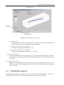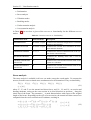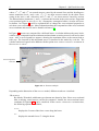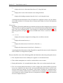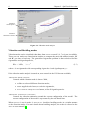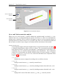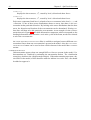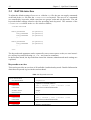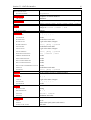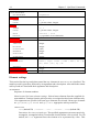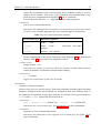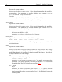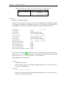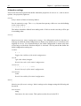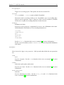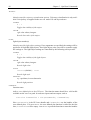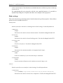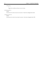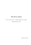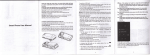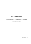
1
SpaVisual User Manual
Steven Boer and Tjeerd van der Poel
2011 Edition, March 14, 2011
Report No. WA-1296
Table of contents
Preface
iii
1
Introduction
1
2
SpaVisual Overview
2.1 Introduction . . . . . . . . . . . . . . . . . . . . . . . . . . . . . . . . . . . .
2.2 Basic controls . . . . . . . . . . . . . . . . . . . . . . . . . . . . . . . . . . .
2.3 Visualization controls . . . . . . . . . . . . . . . . . . . . . . . . . . . . . . .
3
3
3
4
3
SpaVisual Commands
3.1 Introduction . . . . . . . . . . . . . . . . . . . . . . . . . . . . . . . . . . . .
3.2 Options structure interface . . . . . . . . . . . . . . . . . . . . . . . . . . . .
3.3 DAT file interface . . . . . . . . . . . . . . . . . . . . . . . . . . . . . . . . .
11
11
11
12
References
23
i
ii
Table of contents
Preface
This is the 2011 edition of the SPAVISUAL manual for the visualization of SPACAR results in
MATLAB. The SPAVISUAL MATLAB toolbox is developed at the Laboratory of Mechanical
Automation of the Department of Engineering Technology, University of Twente.
The latest version of SPAVISUAL included in the 2011 release of SPACAR, features a graphical user interface unlike previous SPAVISUAL releases. SPAVISUAL makes use of the latest
SPACAR functions and is therefore not backwards compatible with older SPACAR releases. A
new command style, to adjust visualization options, is also implemented. However, for backwards compatibility with ‘old style’ generated dat files, it still supports the old visualization
commands from the visualization tool implemented by Jan Bennik.
March 14, 2011,
ir. S. E. Boer (Email: [email protected]) and dr. ir. G. W. van der Poel.
iii
iv
Preface
1
Introduction
is the visualization tool for SPACAR. It is a stand-alone function in MATLAB and
can visualize deformation, vibration and buckling modes of 2-D and 3-D mechanisms. It can
also visualize over- and underconstaints as well as stresses in beam type elements. SPAVISUAL
shows beams, trusses and hinges (among others) in 2-D as well as in 3-D.
SPAVISUAL
For users new to SPAVISUAL, Chapter 2 gives an overview of all SPAVISUAL functionalities and
limitations and it explains the use of the graphical user interface.
For the more demanding user, a more elaborate overview of the SPAVISUAL commands and
ways to interface with the program, are given in Chapter 3.
1
2
Chapter 1. Introduction
2
SpaVisual Overview
2.1 Introduction
Before a SPAVISUAL call can be made in MATLAB, a call to the SPACAR program must be made
first. This requires the existence of a dat input file that defines the SPACAR model. The output
of a SPACAR run is stored in SPACAR binary data files (SBF). These are files with extensions
sbd, sbm and ltv. Depending on which SPACAR mode is used, the existence of one or more
of these files and the input dat file, is required to run SPAVISUAL. For more information about
the different SPACAR modes, the reader is referred to the SPACAR manual [1]. SPAVISUAL can
be activated with the MATLAB command,
>> spavisual(’filename’)
Here, filename is the name of the dat input file without extensions. Drive or path specifications are not allowed in filename, so the MATLAB working directory should be set to the
location of the dat input file.
In Section 2.2, the basic controls of the graphical user interface options are explained. And in
Section 2.3, an overview is given of the different visualization modes with their controls.
2.2 Basic controls
The basic controls include: the animation of the SPACAR model, the recording of such an animation and how to hide parts of the GUI. In Figure 2.1, these controls are highlighted.
SPAVISUAL MENU
Controls the way the output window is displayed. It has four options,
HIDE UI OBJECTS
Hides the user interface options and controls. Useful for making clean pictures with
the GUI controls removed.
3
4
Chapter 2. SpaVisual Overview
SpaVisual menu
Recording
controls
Animation controls
Figure 2.1: The graphical user interface.
STRETCH TO FILL
Stretches the axis to fill all available space. This option distorts the visualization of
the model as the axis are generally not square anymore.
HIDE AXIS LABELS AND TICK MARKS
Visualizes only the model without the axes.
HIDE STRESS LEGEND AND COLORBAR
Hides stress information when stresses are shown.
ANIMATION CONTROLS
Controls the animation of the model by PLAY and STOP buttons and a slider. If the RE PEAT checkbox is checked, the animation will automatically start again until the checkbox
is cleared.
RECORDING CONTROLS
Options for recording a movie can be found here. By checking the RECORD MOVIE
checkbox, a movie with the supplied movie name will be recorded once the user presses
the PLAY button.
2.3 Visualization controls
Depending on which SPACAR mode is used to run the model, the functionality of
changes and one or more of the following visualization modes can be selected:
SPAVISUAL
Section 2.3. Visualization controls
5
• Deformation
• Stress analysis
• Vibration modes
• Buckling modes
• Underconstraint analysis
• Overconstraint analysis
In Table 2.1, an overview is given of the
modes.
SPAVISUAL
functionality for the different
SPACAR
Table 2.1: Overview SPAVISUAL functionality
Visualization mode
SPACAR mode
Description
DEFORMATION
all modes except 0
Visualizes the deformed configuration as a function
of time or per load step.
STRESS ANALYSIS
all modes except 0
Visualizes the selected stress distribution in beam,
truss and tube elements.
VIBRATION MODES
3, 4, 7, 9
Visualizes the selected vibration mode of the system for the current load step.
BUCKLING MODES
8
Visualizes the buckling mode after a
mode 8 run.
UNDERCONSTRAINT
ANALYSIS
0
Visualizes the selected underconstraint mode of the
system as a vibration.
OVERCONSTRAINT
ANALYSIS
0
Visualizes the selected overconstraint mode of the
system as a stress distribution.
SPACAR
Stress analysis
The stress analysis is available in all SPACAR modes except the zeroth mode. To compute the
stresses, first the cross-sectional stress resultants need to be determined. They are denoted by,
Fx (ξx ),
Fy (ξx ),
Fz (ξx ),
Mx (ξx ),
My (ξx ),
Mz (ξx ),
(2.1)
ξx ∈ [0, 1] ,
where Fx , Fy and Fz are the normal and shear forces, and Mx , My and Mz are torsion and
bending moments, acting on the cross-section in its local directions at position ξx along the
elastic line of the beam. The parameter ξx is made dimensionless with respect to the original
length of the beam. Depending on the type of cross-section, the normal and shear stresses are
computed from the cross-sectional stress resultants, resulting in,
σx (ξx , ξy , ξz ) = σxFx (ξx ) + σxMy (ξx , ξz ) + σxMz (ξx , ξy )
Fy
Mx
τxy (ξx , ξy , ξz ) = τxy
(ξx , ξy ) + τxy
(ξx , ξy , ξz )
Fz
Mx
τxz (ξx , ξy , ξz ) = τxz
(ξx , ξz ) + τxz
(ξx , ξy , ξz )
,
ξy ∈ [−1, 1]
ξz ∈ [−1, 1]
,
(2.2)
6
Chapter 2. SpaVisual Overview
where σxFx , σxMy and σxMy are normal stresses caused by the normal force and the bending moFy
Fz
ments around the local y and z-axis, τxy
, τxz
are shear stresses caused by the shear forces
Mx
Mx
are shear stresses caused by torsion.
acting in the local y and z-direction, and τxy and τxz
The dimensionless parameters ξy and ξz , represent the location in the cross-section. Supported
cross-sectional types in SPAVISUAL are: rectangular, rectangular hollow, circular and circular hollow. In Chapter 3 it will be explained how to change the cross-sectional properties to
suit these cross-sectional types. More information about the computation of the cross-sectional
stress resultants and stresses can be found in reference [2].
In Figure 2.2, stresses are computed for a deflected beam. A colorbar indicates the stress levels,
with its range computed from the minimum and maximum occurring stress for all load or time
steps. Also, a stress legend box appears, showing the maximum stress at the current load or
time step. The location of this maximum stress is visualized in the model by a red dot. The
colorbar and stress legend can be hidden with the option HIDE STRESS LEGEND COLORBAR in
the SPAVISUAL MENU .
Stress component
selection
Figure 2.2: A 3D stress analysis.
Depending on the dimension of the SPACAR model, different results are visualized:
2D
MODELS
By default, 2D models with beam type elements are drawn by lines. Since cross-sectional
data is missing, actual stresses can not be computed. Instead, the cross-sectional stress
resultants of Equation 2.1, can be visualized. In the STRESS COMPONENT selection box,
the following options are available,
Fres
displays the 2-norm of the force vector along the beam
Fx
displays the normal forces Fx along the beam
Section 2.3. Visualization controls
7
Fy
displays the local y-directional shear forces Fy along the beam
Mres
displays the 2-norm of the moment vector along the beam
Mz
displays the bending moments about the local z-axis along the beam
Assuming that the dimensions of the 2D model are supplied in meters [m], the dimension of the colorbar is in Newtons [N] or Newton meter [Nm], for forces and moments
respectively.
3D
MODELS
By default, 3D models with beam type elements are drawn with rectangular cross-sections.
If the user did not explicitly supply the cross-sectional dimensions, default dimensions are
used. The cross-sectional stresses of an element are computed with Equation 2.2. The
following options, see Figure 2.2, are now available in the STRESS COMPONENT selection
box,
von Mises
displays the stresses computed according to the von Mises criterion
sigX
displays the normal stresses, σx
tauXY
displays the shear stresses in the local y-direction, τxy
tauXZ
displays the shear stresses in the local z-direction, τxz
Assuming that the dimensions of the 3D model are supplied in meters [m], the dimension
of the colorbar is in mega Pascals [MPa].
The user should be aware of the following pitfalls and limitations when interpreting the stresses:
• The computed stresses loose validity near supports or concentrated loads
• Thin walled assumptions are used for circular hollow cross-sections
• During deformation, it is assumed that the shape of the cross-section remains the same
• The cross-sectional dimensions that are used to compute the element stiffness properties
in SPACAR, should be the same as the cross-sectional dimensions that are used to visualize the beam type element. For instance, if the elastic constants are computed using a
circular cross-section, and the beam is visualized with a rectangular cross-section, incorrect relations are used to compute the stress components in Equation 2.2, which results in
incorrect computed stresses.
8
Chapter 2. SpaVisual Overview
Vibration
mode options
Vibration
animation controls
Figure 2.3: Vibration mode analysis.
Vibration and Buckling modes
Vibration modes can be visualized when data, from a SPACAR mode 3, 4, 7 or 9 run, is available.
These SPACAR modes use linearization routines to compute the mass and stiffness matrix, M
and K, per time or load step. The generalized eigenvalue problem is then solved to find the
eigenmodes and eigenfrequencies,
Kv = λM v,
λ = ω2
(2.3)
where v is an eigenmode with corresponding eigenvalue λ and eigenfrequency ω.
If the vibration mode analysis is turned on, new controls in the GUI become available,
VIBRATION MODE OPTIONS
Controls which vibration mode is shown. With,
• a slider to selected different vibration modes,
• a user supplied scale factor, to scale the eigenmode,
• a LIST
MODAL FREQUENCIES
button, to list all eigenfrequencies.
VIBRATION ANIMATION CONTROLS
Controls the vibration animation around the current configuration of the model. The
current configuration of the model is represented by the red dotted lines.
When SPACAR is run in mode 8, SPAVISUAL visualizes buckling modes in a similar manner
as the vibration modes. For more details about buckling analysis, the reader is referred to the
SPACAR user manual [1].
Section 2.3. Visualization controls
9
Stress component
selection
Overconstraint
selection
Figure 2.4: Overconstraint analysis.
Over- and Underconstraint analysis
When SPACAR is run in mode 0, it checks whether the supplied model is solvable, i.e. it determines if no over- or underconstraints are present. In SPAVISUAL, these over- and underconstraints can be visualized. This is useful for a designer to achieve an exact constraint design. It
also helps the user to build a correct SPACAR model, since these over- and underconstraint tell
the user where to add or remove degrees of freedom (DOFs) and releases in the model.
OVERCONSTRAINTS
Overconstraints appear when not enough releases are present in the model. In Figure 2.4,
a clamped-clamped beam with no releases is shown. The overconstraint analysis determines that the model is six times overconstraint. To determine how to solve these overconstraints, they are visualized using imaginary stress distributions. The visualization
controls for overconstraints are therefor similar to those of a stress analysis. It features
a STRESS COMPONENT SELECTION box, where the individual stress components from
Equation 2.2 can be selected,
von Mises
displays the stresses computed according to the von Mises criterion
sigX Fx
displays normal stresses, σxF x , caused by normal forces.
sigX My
displays normal stresses, σxM y , caused by bending moments about the local y-axis.
sigX Mz
displays normal stresses, σxM z , caused by bending moments about the local z-axis.
tau Mx
Mx
Mx
, caused by torsion.
and τxz
displays the 2-norm of the shear stresses, τxy
10
Chapter 2. SpaVisual Overview
tauXY Fy
Fy
displays the shear stresses, τxy
, caused by local y-directional shear forces.
tauXZ Fz
Fz
displays the shear stresses, τxz
, caused by local z-directional shear forces.
Each stress component listed here is related to forces or moments in the local x-, y- and
z-direction. If one of these stress distributions shows no stress, then there is no overconstraint in that particular direction. By looking at the stress distributions that do show
stress, the direction and location of the overconstraint can be determined. Placing a release here will then solve this particular overconstraint. As an example, for the overconstraint shown in Figure 2.4, the third deformation component, which corresponds to the
bending deformation mode about the z-axis at the p-side of the beam, needs to be released
to solve the overconstraint.
An OVERCONSTRAINT SELECTION slider is available to navigate between different overconstraints if more than one overconstraint is present in the model. Also, the LIST OVER CONSTRAINTS button can be used to show which elements in the model have overconstraints.
UNDERCONSTRAINTS
Underconstraints appear when not enough DOFs or fixes are present in the model. Underconstraints are visualized by animating the unconstraint motion. The visualization
controls are similar to the vibration mode analysis. If the underconstraint represents a desired DOF in the model, a DOF should be added to indicate it as such. Else, a fix should
be added to suppress it.
3
SpaVisual Commands
3.1 Introduction
Asides from the GUI, there are more ways to interface with SPAVISUAL. Settings can be
changed by supplying an additional options parameter when calling SPAVISUAL, or they can
be predefined in the dat input file. Both methods will be explained in Section 3.2 and Section 3.3 respectively.
The types of settings that can be changed through the options structure or the dat file, are
• Element settings Includes settings that can change the cross-sectional properties like the
element shape and dimensions, and graphical properties such as color and lighting.
• Animation settings Controls the way the model is animated. Here among others, figure
axis settings and movie settings can be supplied.
• Mode settings Controls the way the different visualization outputs behave. Most options
given here can also be changed in the GUI.
3.2 Options structure interface
Documentation for these options to come in future releases.
11
12
Chapter 3. SpaVisual Commands
3.3 DAT file interface
To adjust the default settings of SPAVISUAL with the dat file, the user can supply commands
at the end of the dat file after the VISUALIZATION keyword. The SPAVISUAL commands
are controlled by keywords, which come into two groups: main and sub keywords. The sub
keywords define settings related to the first preceding main keyword. The structure of the
VISUALIZATION block in the dat file is then as follows,
VISUALIZATION
MAIN_KEYWORD
SUB_KEYWORD
SUB_KEYWORD
...
(arguments)
(arguments)
(arguments)
MAIN_KEYWORD
SUB_KEYWORD
...
(arguments)
(arguments)
etc.
The keywords and arguments can be separated by one or more spaces or tabs, are case insensitive and any keywords following a #, % or ; are treated as comments.
In the Sections ahead, the keywords that control the element, animation and mode settings are
explained.
Keywords overview
This section provides an overview of all available visualization keywords. Detailed information
about these keywords is given in the sections ahead.
Table 3.1: Keywords overview
MAIN KEYWORDS
SUB KEYWORDS
BEAMPROPS
arguments
sequence of element numbers
CROSSTYPE
rect | recthol | circ | circhol | line
CROSSDIM
NUMSECTIONS
list of cross-sectional dimensions
integer
SHOWJOINTS
0 | 1
TRUSSPROPS
sequence of element numbers
CROSSTYPE
rect | recthol | circ | circhol | line
CROSSDIM
list of cross-sectional dimensions
HINGEPROPS
CROSSDIM
sequence of element numbers
diameter and thickness
Section 3.3. DAT file interface
13
MAIN KEYWORDS
SUB KEYWORDS
WHEELPROPS
CROSSDIM
DONOTDRAW
arguments
sequence of element numbers
thickness
sequence of element numbers or one of the following strings:
beam | rbeam | tube | truss | hinge | wheel | plbelt
MESH
TOT
X , Y, Z , R , PHI
GRAPHICS
sequence of element numbers
integer or: coarse | normal | fine
integer
sequence of element numbers
LINESTYLE
- | -- | : | -.
LINEWIDTH
EDGECOLOR
scalar
scalar between 0 and 1
r g b color values, integers
EDGELIGHTING
flat | phong | gouraud
FACEALPHA
FACECOLOR
scalar between 0 and 1
r g b color values, integers
FACELIGHTING
flat | phong | gouraud
BACKFACELIGHTING
lit | reverse | unlit
AMBIENTSTRENGTH
OPACITY
scalar
scalar
scalar
scalar
scalar
scalar between 0 and 1
LIGHTING
flat | phong | gouraud
EDGEALPHA
DIFFUSESTRENGTH
SPECULARSTRENGTH
SPECULAREXPONENT
SPECULARCOLORREFLECTANCE
RANGE
m-by-1 matrix of time or load step indices
INITIAL
VISIBLE
0 | 1
COLOR
r g b color values, integers
LINESTYLE
- | -- | : | -.
LINEWIDTH
scalar
MOVIE
RECORDMOVIE
string
0 | 1
AVITYPE
matlab | videoIO
AVIOPTS
fieldname and value
MOVIENAME
AXISPROPS
VIEW
LIMITS
XLIM , YLIM , ZLIM
az el
xmin xmax ymin ymax (zmin zmax)
min max
14
Chapter 3. SpaVisual Commands
MAIN KEYWORDS
SUB KEYWORDS
arguments
TRAJECT
VISIBLE
0 | 1
COLOR
r g b color values, integers
LIGHT
VISIBLE
0 | 1
COLOR
r g b color values, integers
STYLE
infinite | local
POSITION
x y z positions, in axes data units
function name
USERPLOT
MODESHAPE
VIBRATION
BUCKLING
SCALEFACTOR
MAXIMUM
NUMCYCLES
NUMFRAMES
integer
integer
scalar
integer
scalar
integer
STRESS
COMPONENT
mises | sigX | tauXY | tauXZ | Fres | Fx | Fy
Fz | Mres | Mx | My | Mz
SHOWMAX
0 | 1
OVERCONSTRAINT
integer
UNDERCONSTRAINT
integer
Element settings
This section lists the keywords that control the way elements in SPAVISUAL are visualized. The
main keyword is given first, followed by its arguments and a description. After which the related
sub keywords are listed with their arguments and description.
BEAMPROPS
Sequence of element numbers.
Main keyword for beam element settings. Selects beam elements from the supplied element numbers. Settings from the sub keywords, are assigned to these beam elements only.
If no arguments are specified, all beam type elements are selected. Beam type elements
are (pl)beam, (pl)rbeam and (pl)tube. Appropriate sub keywords are:
CROSSTYPE
rect (default 3D) | recthol | circ | circhol | line (default 2D)
Determines the cross-sectional type. The specified arguments represent respectively,
rectangular, rectangular hollow, circular and circular hollow cross-sections. For 3D
models, the line argument forces the element to be represented by a line. This
Section 3.3. DAT file interface
15
allows the visualization of the cross-sectional stress resultants, similar to a stress
analysis for 2D models. Vice-versa, if for 2D models cross-sectional data is supplied, the stress components from Equation 2.2 can be visualized.
It is not allowed to mix the line argument, with the other arguments.
CROSSDIM
List of cross-sectional dimensions.
Determines the dimensions for the supplied cross-sectional type in the beam element
local directions. Possible arguments per cross-sectional type are listed below.
Table 3.2: Cross-sectional dimension arguments
Cross-sectional type
Dimension arguments
rect
height
width
recthol
height
width
circ
diameter
circhol
diameter
inner-height
inner-width
inner-diameter
For the computation of the stress components from Equation 2.2, the dimensions
listed in Table 3.2 are assumed to be supplied in meters.
NUMSECTIONS
integer (default = 10)
Determines the number of sections in which the element is divided. More sections,
results in smoother visualization of beams under bending.
SHOWJOINTS
0 | 1 (default)
Toggles the visualization of joints for 2D beams.
TRUSSPROPS
Sequence of element numbers.
Main keyword for truss element settings. Selects truss elements from the supplied element
numbers. Settings from the sub keywords, are assigned to these truss elements only. If
no arguments are specified, all truss type elements are selected. Truss type elements are
truss and pltruss. Appropriate sub keywords are:
CROSSTYPE
rect | recthol | circ (default 3D) | circhol | line (default 2D)
Determines the cross-sectional type. See BEAMPROPS for more information.
CROSSDIM
Sequence of cross-sectional dimensions.
Determines the dimensions for the supplied cross-sectional type. See Table 3.2 for
more information.
16
Chapter 3. SpaVisual Commands
HINGEPROPS
Sequence of element numbers.
Main keyword for hinge element settings. Selects hinge elements from the supplied element numbers. If no arguments are specified, all hinge type elements, hinge and
pltor, are selected. Its only sub keyword is:
CROSSDIM
diameter (default = 0.01) and thickness scalar (default = 0.002).
Determines the diameter and thickness of the selected hinge elements.
WHEELPROPS
Sequence of element numbers.
Main keyword for wheel element settings. Selects wheel elements from the supplied element numbers. If no arguments are specified, all wheel type elements, wheel and
plwheel, are selected. Its only sub keyword is:
CROSSDIM
thickness scalar (default = 0.002)
Determines the thickness of the selected wheel elements.
DONOTDRAW
Sequence of element numbers or one of the following strings
beam | rbeam | tube | truss | hinge | wheel | plbelt
Determines which elements not to draw. The string arguments, also work for their 2D
equivalent elements.
MESH
Sequence of element numbers.
Main keyword for mesh settings of beam type elements for stress analysis. Mesh settings
are assigned to beam or truss type elements from the supplied element numbers. The
mesh settings determine the number of evaluation points in the elements. The following
sub keywords control the mesh settings:
TOT
integer or one of the following strings
coarse | normal | fine
Determines the total amount of evaluation points. The number of evaluation points
represented by the string arguments, is different for the 1D line cross-sectional
type and the other 2D cross-sectional types, see Table 3.3.
X , Y, Z , R , PHI
integer
Determines the amount of evaluation points in the x-, y-, z-, radial or rotational
direction. If one or more of these sub keywords are not specified, values are assigned automatically to have an aspect ratio of about 1 for the distance between the
evaluation points.
Section 3.3. DAT file interface
17
Table 3.3: Number of evaluation points represented by the string arguments
Cross-section dimension
coarse
normal
fine
1D
5
50 (default)
100
2D
100
1000 (default)
10000
GRAPHICS
Sequence of element numbers.
Main keyword for graphics settings of elements. If no arguments are specified, the graphics settings are assigned to all elements in the model. The sub keywords determine element lighting, color and other graphical properties. Supported sub keywords are:
LINESTYLE
- | -- | : | -. | none
LINEWIDTH
EDGECOLOR
scalar
scalar between 0 and 1
r g b color values, integers
EDGELIGHTING
flat | phong | gouraud
FACEALPHA
scalar between 0 and 1
r g b color values, integers
EDGEALPHA
FACECOLOR
FACELIGHTING
BACKFACELIGHTING
AMBIENTSTRENGTH
DIFFUSESTRENGTH
SPECULARSTRENGTH
SPECULAREXPONENT
SPECULARCOLORREFLECTANCE
flat | phong | gouraud
lit | reverse | unlit
scalar
scalar
scalar
scalar
scalar
See the MATLAB manual [3] on patch properties for more information on these sub keywords. If the line cross-sectional type is used (default for 2D models), only the sub
keywords LINESTYLE , LINEWIDTH and FACECOLOR function.
Other graphical sub keywords are,
OPACITY
scalar between 0 and 1.
Changes element opacity. This option changes both the EDGEALPHA and FACEAL PHA option simultaneously.
LIGHTING
flat | phong | gouraud
Changes element lighting. This option changes both the EDGELIGHTING and FACE LIGHTING option simultaneously.
18
Chapter 3. SpaVisual Commands
Animation settings
This section lists the keywords that define animation properties of
options, axis properties, lights etc.
SPAVISUAL,
such as movie
RANGE
m-by-1 matrix of time or load step indices.
Sets the animation range. The range keyword accepts any valid MATLAB code defining
a row vector, such as:
2:2:10 or [1 4 6 ...]
The indices should be defined in ascending order. If this is not the case they will be put
in ascending order.
INITIAL
Main keyword for initial configuration settings. For deformation analysis, the time or
load step at which the initial configuration is drawn, is by default set to 1 or the first value
supplied in RANGE . For vibration analysis, the initial configuration is drawn at the time
or load step at which the vibration analysis is activated. Sub keywords that define the
initial configuration settings are:
VISIBLE
0 | 1
Toggles the visibility of the initial configuration.
COLOR
r g b color values, integers.
Sets the line color of the initial configuration.
LINESTYLE
- | -- | : | -. | none
Sets the line style of the initial configuration.
LINEWIDTH
scalar
Sets the line width of the initial configuration.
MOVIE
Main keyword for movie settings. Movie settings can be changes using the following sub
keywords:
MOVIENAME
string
Determines the movie name. This option can also be set in the GUI.
Section 3.3. DAT file interface
19
RECORDMOVIE
0 | 1
Toggles the recording option. This option can also be set in the GUI.
AVITYPE
matlab (default) | videoIO (only available if installed)
Determines which recording toolbox to use. By default, MATLAB recording functions are used to generate a movie. However, if the VIDEO IO toolbox is available
on the MATLAB path, its recording functions can also be used.
AVIOPTS
fieldname and value.
Sets the avi object properties. Arguments for AVIOPTS are a fieldname with a value.
Valid fieldnames for default MATLAB recording functions are:
colormap
compression
fps
keyframe
quality
videoname
See the avifile function in the MATLAB manual [3] for more information.
For the VIDEO IO toolbox, see the videowriter function for possible fieldnames
with values.
AXISPROPS
Main keyword for figure axes properties. Sub keywords that define the axes properties
are:
VIEW
az el
Sets the viewpoint. See the view function in the
information.
MATLAB
manual [3] for more
MATLAB
manual [3] for more
LIMITS
xmin xmax ymin ymax (zmin zmax)
Sets the axes limits. See the axis function in the
information.
XLIM , YLIM , ZLIM
min max
Sets the individual axis limits. See the xlim, ylim and zlim functions in the
MATLAB manual [3] for more information.
20
Chapter 3. SpaVisual Commands
TRAJECT
Main keyword for trajectory visualization options. Trajectory visualization is only available if a trajectory is supplied in the SPACAR model. Its sub keywords are:
VISIBLE
0 | 1
Toggles the visibility of the traject.
COLOR
r g b color values, integers.
Sets the line color of the traject.
LIGHT
light object number(s)
Main keyword for light object settings. If no arguments are specified, the settings will be
applied to all available light objects. If no light objects exist, one will be created to apply
the settings to. The light object settings are controlled by the following sub keywords:
VISIBLE
0 | 1
Toggles the visibility of the light objects.
COLOR
r g b color values, integers.
Sets the light color.
STYLE
infinite (default) | local
Sets the light style.
POSITION
x y z positions, in axes data units.
Sets the light position.
USERPLOT
function name
Adds a user defined plot to the GUI axes. The function name should be a valid m-file
available on the MATLAB path. It needs two inputs and one output, such as
function funHandles = fun(axesHandle, funHandles)
Here axesHandle is the GUI axes handle and funHandles are the handles of the
user defined plots. If in SPAVISUAL, the user defined plot function is called for the first
time, funHandles will be empty. SPAVISUAL expects the function to return the handles
Section 3.3. DAT file interface
21
of the created objects. Note that the user defined function is called every time or load step
in SPAVISUAL.
By manipulating the axes properties with the user supplied function, it is possible to
dynamically change the viewpoint and other axes settings as time progresses.
Mode settings
This section lists the keywords that control visualization mode specific properties. Most of these
options are also available in the GUI.
MODESHAPE
Main keyword for vibration or buckling mode related settings. Its sub keywords are:
VIBRATION
integer
Determines the initial selected vibration mode. Can also be changed in the GUI.
BUCKLING
integer
Determines the initial selected buckling mode. Can also be changed in the GUI.
SCALEFACTOR
scalar
Sets the scale factor. Can also be changed in the GUI.
MAXIMUM
integer
Determines the maximum number of computed mode shapes.
NUMCYCLES
scalar
Scales the amount of cycles the mode shape is animated.
NUMFRAMES
integer
Sets the amount of frames used to animate one mode shape cycle.
STRESS
Main keyword for stress analysis related settings. Its sub keywords are:
COMPONENT
mises (default)|sigX|tauXY|tauXZ|Fres|Fx|Fy|Fz|Mres|Mx|My|Mz
Determines the initial selected stress component. Can also be changed in the GUI.
22
Chapter 3. SpaVisual Commands
SHOWMAX
0 | 1
Toggles the visibility of the max stress location.
OVERCONSTRAINT
integer
Determines the initial selected overconstraint. Can also be changed in the GUI.
UNDERCONSTRAINT
integer
Determines the initial selected underconstraint. Can also be changed in the GUI.
References
[1] Aarts, R. G. K. M., Meijaard, J. P., Jonker, J. B., SPACAR User Manual 2009, Technical
Report WA-1180, University of Twente, Faculty of Engineering Technology, Mechanical
Automation Labarotory, March 2009.
[2] Boer, S. E., Aarts, R. G. K. M., Brouwer, D. M., Jonker, J. B., Multibody Modelling and
Optimization of a Curved Hinge Flexure, In The 1st Joint International Conference on
Multibody System Dynamics, Lappeenranta, Finland, May 25-27, 2010.
[3] The Math Works Inc., Getting Started with MATLAB, version 7, Revised for MATLAB 7.1
(Release 14SP3), September 2005.
23