1
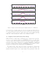
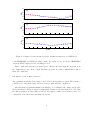
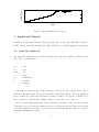
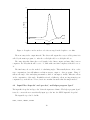
User’s Manual for NEARCOM Diffractive, Unsteady
Wave Driver DUNS
Andrew B. Kennedy
Department of Civil and Coastal Engineering
University of Florida, Gainesville, FL 32611-6590 USA.
[email protected]
&
James T. Kirby
Center for Applied Coastal Research
University of Delaware, Newark, DE 19716 USA.
[email protected]
1
1
Summary
This manual gives a brief description of the diffractive, unsteady wave driver DUNS for the
NEARCOM model suite. Examples and sample setups are included. The model can predict
leading order time-varying, multidirectional, and diffractive behaviour and is thus expected to be
useful for the study of wave group forcing on nearshore hydrodynamics. Leading order, but not
full, wave-current interaction is included. Because of assumptions in the derivation and choices
made in coding, the model is meant for use on open beaches where there is a clear longshore and
cross-shore direction. It should not be used in areas with strongly curved shorelines or in areas
with strong diffraction, such as inside a harbor.
2
2
Introduction
Waves in the ocean are universally acknowledged to be unsteady and multidirectional. As they
pass from deep water into finite depths and through to the shoreline, these variations in shoaling
and breaking wave heights and directions will also cause spatial and temporal variations in low
frequency waves and currents. Despite this, the majority of numerical modelling efforts have used
either monochromatic or spectral models, neither of which includes the effects of wave groups.
In this manual, we describe a numerical wave driver, DUNS, that can describe the time-varying
wave climate in the nearshore on the scale of wave groups. The model operates in the time domain
and includes leading order multidirectionality, diffraction, and wave-current interaction. The basic formulation is from Kennedy and Kirby (2003), and comes from a nonlinear, multiple scale
perturbation expansion. Multidirectionality and diffraction are accounted for by making the wave
amplitude, A, complex with both real and imaginary components. This leading order multidirectionality is accurate to approximately ±30 degrees from a central direction, and diffractive
frequency dispersion to perhaps ±15% from a peak frequency. Accuracy degrades continuously
from this peak direction and frequency, but is quite accurate near the peak.
2.1
Numerical Setup
All waves are generated at the offshore boundary as seen in Figure 1. Offshore waves may have
any mean angle where the waves travel into the domain rather than out of the domain - this is
to say that the waves must travel somewhat in the positive x-direction rather than the negative
x-direction.
The driver has an unstaggered grid and is second order in space and fourth order in time.
Differences are centered in space.
The main evolution equation solved by the driver is:
"
2At + 2(C̄g ) · ∇A + σ̄∇ ·
C̄g
−i ∇2 A + i
κ̄
C̄g
− σ̄κ̄κ̄
κ̄
!
C̄g
σ̄
!
#
1
− σ̄t A − 2iA C̄g (κ − κ̄) + κ̂ · Ū
σ̄
Axx k̄ 2 + 2Axy k̄ l̄ + Ayy l̄2
κ¯2
!
+ iσ̄κ̄2 β|A2 |A
+2w = 0
(1)
where κ̄ is the regularised bathymetry, and κ̂ ≡ (κ − κ̄)(cos θ, sin θ) is the difference between
the actual and regularised wavenumbers multiplied by the wave direction vector.
The regularised wavenumber k̄ is taken from the regularised depth h̄. This is defined as any
depth field for which the underlying wavenumber vector field has no caustics: many topographies
with submerged shoals will not have well behaved refraction fields, so a regularised bathymetry
3
Onshore boundary
==> y
Offshore boundary
Lateral boundary
0
==> x
Lateral boundary
Figure 1: Definition sketch for wave propagation showing boundaries and sample wavenumbers in
the domain.
is defined with acceptable refraction. The regularised wavenumber vector field satisfies the linear
dispersion relation
σ 2 = gκ̄ tanh κ̄h̄
(2)
and the eikonal wavenumber condition ∇ × (κ̄(cos θ, sin θ)) = 0.
The difference between the regularised and actual bathymetries drives diffractive terms which
approximate the effects of the actual bathymetry. This approach has been known for some time
and is used in well known models such as REF/DIF1. In DUNS, the regularised bathymetry
is computed at each x-location as the longshore average (in y) of the depth. This is the main
reason that restricts DUNS to open beaches, and is a coding choice, not a theoretical restriction.
Considerably more complex choices could be used as long as they satisfy the eikonal wavenumber
relations, but would require some recoding. The closer the regularised bathymetry is to the actual
bathymetry, the more accurate the program becomes.
The group velocity Cg ≡ ∂σ/∂κ and the diffractive coefficient σ κ̄κ̄ and nonlinear dispersion
coefficient β are defined in Kennedy and Kirby (2003).
Wave dissipation is represented in equation (1) by w and is taken as that of Roelvink (1993),
4
but would be simple to change to any other desired formulation.
The program is written in mainly standard fortran77, but on some compilers you will need
to compile it as a f90 code because of non-standard extensions. Sample compiler commands are
included in section 4.5. Memory requirements are not large and it can be run easily on any modern
PC.
Because DUNS operates in the time domain, it is different from most of the wave drivers that
operate with NEARCOM. The majority of these provide steady radiation stresses which force the
circulation components for a period of minutes to an hour, at which time a new wave climate
might be applied. For wave group forcing, this is not at all acceptable. Wave group time scales
are generally defined to be of O(20-200s), so to resolve the temporal variation of wave forcing
to the circulation model, we must update on time scales much less than this. Typically, we
recommend passing information to the circulation model at time scales of O(1-2s) to ensure good
resolution. Those with quick eyes will note that this gives the overall model first order accuracy
on the time scale of the information passing (1-2s). Because of the modular NEARCOM design,
this is unavoidable, but errors introduced here are probably order of magnitude less than errors
in estimating, for example, radiation stresses in breaking waves.
3
3.1
Examples
Wave focusing on a submerged shoal
This is a nonbreaking example that can not be duplicated here because of the wave breaking in
the code, but serves to evaluate the accuracy of the basic formulation. The focusing shoal of
Berkhoff, Booiy, and Radder (1982) has been used as a test of difraction for many different wave
models. Figure 2 shows the bathymetry contours and measurement cross-sections.
This topography leads to strong focusing of wave rays, with caustics occurring behind the
shoal. Because of this, method 1 may not be used on this topography, as an underlying refraction
solution does not exist. However, method 2 is well suited to such a computation. The underlying
bathymetry was assumed to be a longshore uniform beach, whose depth was chosen to be the
average over the longshore domain. A computational grid size of ∆x = ∆y = 0.25m was used with
a time step of ∆t = 0.025s. Lateral boundaries used a reflective condition, which is considerably
different than the physical experiment, but as boundaries were far away from the area of interest,
this was not a concern.
Formally, the physical wave height in computations is not just H = 2|A|, but includes higher
order corrections. However, because of the semi-empirical modifications to nonlinear dispersion,
with unknown effects on surface profiles, we use this simpler representation. For some situations,
5
25
20
(8)
(7)
(6)
8
10
12
(5)
Distance (m)
(4)
(3)
15
(2)
(1)
10
5
0
0
2
4
6
14
16
18
20
Distance (m)
Figure 2: Contours of bathymetry on BBR shoal, showing measurement transects.
this approximation would be unacceptably crude; however, for the present case, reasonable results
may still be obtained.
Figures 3-4 show computed and measured wave heights along the transects. In general, agreement is quite good. Both the trend and the magnitude of the refraction and diffraction caused
by the shoal are well represented. The present results look very similar to those computed using
the narrow angle parabolic model given in Kirby and Dalrymple (1986). This is not surprising as,
with the further assumptions of time invariance, weak diffraction in the direction of propagation,
and negligible current, the two models are equivalent. Since none of these effects are likely to be
highly significant in this case, the results are very similar.
Although the present results are good, it is possible to achieve slightly greater accuracy by using
full time-domain systems such as Boussinesq models (e.g., Wei et al., 1995). This is because these
models do not assume an underlying form for the wave, and thus can represent better the strong
nonlinear diffraction. Still, Boussinesq models are computationally an order of magnitude slower
than the present model, and thus cannot be easily used for long time scales in field situations.
Wide-angle parabolic models can also produce slightly better results in this case (e.g. Kirby,
1986), as their treatment of diffraction is more accurate. This improvement in accuracy is mainly
6
(1)
H/H0
2
1
0
5
6
7
8
9
10
11
12
13
14
15
6
7
8
9
10
11
12
13
14
15
6
7
8
9
10
11
12
13
14
15
6
7
8
9
10
11
12
13
14
15
6
7
8
9
10
11
12
13
14
15
(2)
H/H0
2
1
0
5
(3)
H/H0
2
1
0
5
(4)
H/H0
2
1
0
5
(5)
H/H0
2
1
0
5
y (m)
Figure 3: Computed (-) and measured (x) wave heights at transects 1-5 on BBR shoal
seen in the side lobes of longshore transects 4-5, where the wide-angle approximation allows for
more accurate diffraction far from the mean wave direction. Overall, however, agreement is quite
good using the present model, and gives confidence that accurate refraction/diffraction/shoaling
results can be obtained in situations for which no direct confirmation is available.
3.2
Longshore Current with Unsteady Wave Forcing
DUNS is well suited to examine longshore currents in the presence of unsteady wave forcing. Here,
it is used to force the quasi-3D circulation model SHORECIRC (Svendsen et al., 2002). Figure
5 shows the longshore-uniform bathymetry, which has a bar-trough topography. This example is
found in the download package. All input files for both DUNS, SHORECIRC, and NEARCOM
are included. A dummy sediment module is used. SHORECIRC here is used in 2D mode, as there
are unresolved feedback issues between DUNS and the 3D SHORECIRC flow.
The example is a little contrived, with only 5 frequency components used, so that users may
see easily how the program works and may also modify it easily. Still, it shows many of the
principles and methods required for more complex examples. The program runs for 1200 s, with
7
2.5
(6)
H/H0
2
1.5
1
0.5
0
0
1
2
3
4
5
6
7
8
9
10
11
1
2
3
4
5
6
7
8
9
10
11
1
2
3
4
5
6
7
8
9
10
11
2.5
(7)
H/H0
2
1.5
1
0.5
0
0
2.5
(8)
H/H0
2
1.5
1
0.5
0
0
x (m)
Figure 4: Computed (-) and measured (x) wave heights at transects 6-8 on BBR shoal
both SHORECIRC and DUNS providing output. We will not worry about the SHORECIRC
output as DUNS output provides everything we need.
First, compile and run helper program, ‘fgen.f’. This produces the input file ‘freqs.dat’ from
the original file spec.dat’. Next, compile the master program. A compile command that works on
many PC compilers is
f90 master.f sed.f duns.f winc*.f
Any optimization switches desired may be used. Next, run the master program. There must be
a subdirectory ‘data’ in the target directory as the program will write output here.
After the master program has finished, the Matlab code ‘readata.m’ will compute and plot the
mean current and vorticity averaged from 800-1200s. Results are shown in figures 6-7. Note that
the 400s averaging period has still not removed all longshore variation in vorticity because of a
combination of the shear waves and unsteady forcing.
8
Elevation (m)
0
−2
−4
−6
0
50
100
150
200
250
x (m)
Figure 5: Barred bathymetry for test case.
4
Inputs and Outputs
In addition to data passed from the master program, there are two major input files required by
DUNS. One gives general computational details, while the second details input wave parameters.
4.1
Input File ‘winput.dat’
The input file ‘winput.dat’ provides the grid sizes, time step, and boundary conditions for the
wave driver. A sample file is
3.0
10
0.25
3
15
1
1
! cdx
! cdy
! cdt
! mbcy
! ncallskip
! I_hard
! Ang_use
The first two entries are the x and y grid sizes, cdx and cdy. Theoretically, these could be
taken from the master grid, but we find it useful to make them explicit. The next quantity is
the model time step. The next is the lateral boundary condition: for a periodic boundary, set to
mbcy=3, while for a lateral wall boundary condition on both sides, set to mbcy=1.
We note very strongly that the size of the domain will be different for wall or periodic boundary
conditions: for a periodic lateral domain, the size is ny ∗ dy (as in a discrete Fourier series), while
for a wall domain, the size is (ny − 1) ∗ dy (because the first and last grid points are exactly at
the walls in an unstaggered grid).
9
1.2
1
U, V (m/s)
0.8
0.6
0.4
0.2
0
−0.2
0
50
100
150
200
250
x (m)
Figure 6: Longshore and cross-shore velocities averaged in the longshore over 400s.
The next entry is the output interval. The driver will output files every ncallskip times it is
called by the master program, i.e. after the ncallskipth call, 2 ∗ ncallskipth call, etc.
The entry after this defines the record length for the binary output, and may differ between
computers. For PCs, this should be set to ‘1’, while with some unix compilers, it should be set to
‘4’.
The final entry chooses the method of calculating angles. This actually has no effect on the
wave computations, but will influence radiation stresses output to other programs. Using ‘1’
will use the angle of the underlying wavenumber, while ‘2’ attempts to include diffractive effects
on the computation of the angle. If multidirectional or diffractive effects are important in your
computation, you should use ‘2’ here, but it is somewhat less stable that the simple method.
4.2
Input Files ‘freqs.dat’ and ‘spec.dat’, and helper program ‘fgen.f ’
The input file ‘freqs.dat’ and ‘spec.dat’ define the input wave climate. The helper program ‘fgen.f’
is used to convert the more user-friendly input ‘spec.dat’ into the DUNS input file ‘freqs.dat’.
The input file ‘spec.dat’ looks like
9300, 22332, 49992, 32244
10
900
800
700
y (m)
600
500
400
300
200
100
0
0
50
100
150
200
x (m)
Figure 7: Vorticity averaged over 400s. Note the presence of shear waves is still noticeable because
of the relatively short averaging period.
8
6.0
0.15
0.0 10.0
0.1425 0.4 10.0
0.141 0.15 8.0
0.159 0.15 13.0
0.1308 0.15 20.0
0.1712 0.15 7.0
0.155 0.15 10
0.165 0.15 0
The first four entries are seeds for a random number generator used to generate phases for
each component. They may be changed as desired. The next entry is the number of frequency
components to be used. (The maximum number of entries is governed by ‘maxfreq’ in ‘p1.h’, and
is initially set to 501. This can be changed if desired.) The line after this is the depth at which
these will be generated (depth at offshore boundary). Each of the next lines contains data about
each of the unsteady components. The first number on each line is the frequency in Hz. The
second is the amplitude of each component in m. The third is the orientation of each component
11
relative to the x-axis in degrees (0 is exactly oriented with the x-axis).
This is quite simple, but there are several subtleties:
• The first component encountered in the file will be taken to provide the central frequency
and direction. Note that by giving it zero amplitude here, we can define it without messing
up any other ordering scheme for frequencies we may wish to use.
• If a wall lateral boundary condition is used, (mbcy=1), all components are set to have zero
angle,
• The program ‘fgen.f’ assigns a random phase to each component. These are set by the
constants at the beginning of the program and can be changed if desired,
• For a periodic boundary condition and a given wavelength, there are only a limited number
of angles that are physically possible. For an overall longshore domain length of L y0 = ny∗dy
the fundamental longshore wavenumber is then k y0 = 2π/Ly0 . Every wave component must
then satisfy kj sin θj = mky0 , where kj and θj are the wavenumber and angles of component
j, and m is an integer. This is checked in the main program and angles are adjusted to fit
properly. Sometimes the jump from one allowable angle to another may be more than might
be tolerable: in these cases, it is best to increase the longshore domain length, if possible.
4.3
Output after each wave driver call
At the end of each wave driver call when control returns to the master program, DUNS outputs
several ascii files that are useful for examining wave output. These are of the form ‘junk?.out’,
where ‘?’ is an integer. η, Ū , A, and V̄ correspond to ? = 1 − 4. The format of the output is
100
open(1,file=’junk1.out’)
do i = 1, nx
write(1,100)(etac(i,j),j=1,ny)
end do
close(1)
format(401(f10.4))
These can be loaded directly into Matlab or other programs, or they may be viewed using a text
editor. Because they always have the same name, they are overwritten every time the wave driver
is called.
12
4.4
Output After Every ncallwave Times the Wave Driver is Called
Binary data files are written to the ‘data’ subdirectory every ncallwaveth time the wave driver
is called, or every ncallwave ∗ master dt ∗ n interval callwave seconds. These have the form
‘amp00001.out’ and so on where ‘amp’ is replaced by ‘eta’, ‘u’, or ‘v’ for other variables. The files
are written using the commands
&
&
&
&
write(fnames,’(a8,i1,i1,i1,i1,i1,a4)’)’data/amp’,
mod(noutskip/10000,10), mod(noutskip/1000,10),
mod(noutskip/100,10),
mod(noutskip/10,10),mod(noutskip,10),’.out’
open(1,file= fnames, status = ’unknown’,
access=’direct’, recl=4*ny)
do i = 1, nx
write(1,rec=i),(abs(amp(i,j)), j=1,ny)
end do
close(1)
where noutskip = 1, 2, 3, . . . numbers the files sequentially. These files may be read using fortran
or Matlab.
If different output data is desired, probably the easiest way is to add another output section
similar to that above but with the appropriate filename and output variable. For example, to
output radiation stress Sxx ,
c
write(fnames,’(a8,i1,i1,i1,i1,i1,a4)’)’data/sxx’,
middle lines the same
do i = 1, nx
write(1,rec=i),(pass_sxx(i,j), j=1,ny)
end do
close(1)
is appropriate. Note that the ‘a8’ on the first line would have to be changed if the filename prefix is not three letters like ‘sxx’. Other possible desired outputs are pass sxy, pass syy, pass theta,
pass ubott, pass height, pass cg, pass wavenum, pass theta, pass c, pass massf luxu, pass massf luxv,
pass diss, pass wavef y, pass wavef x. Not all of these change with time, so outputting some
would be wasteful.
13
4.5
Compilation and Execution
A compile command that works on many PC compilers is
f90 master.f sed.f duns.f winc*.f
where ‘duns.f’ is the DUNS code. Any optimization switches desired may be used.
To compile the helper program ‘fgen’, the command
f90 fgen.f
works. ‘Fgen’ may also be compiled as a fortran77 program.
To execute, simply run the ‘master’ program using whatever format is best on the particular
system. I find that, on a PC, running in a DOS window is much better, as if the program can’t
read input or blows up for any reason, the window doesn’t disappear. On Unix or Linux shells,
this should not be a problem.
5
How to get Bad Results
These are a few ways in which you can get bad results from the wave driver.
5.1
No ‘data’ subdirectory
If you do not have a ‘data’ subdirectory for out put data, you will get an error the first time the
program tries to write sequential files.
5.2
Short longshore domain
If you have a short longshore domain, the mean angle will not be represented well (because of the
finite number of possible angles for a given wavenumber in a finite longshore domain). To fix this,
increase domain length.
5.3
Very strong longshore bathymetry variations
This program is coded only for mild longshore bathymetry variations. It is difficult to define
‘mild’ exactly, but a good rule of thumb might be that for a constant x, longshore depths should
not vary from the mean longshore depth at that location by more than a factor of 2. For very
strong longshore variations, you will continue to get results, but these will become increasingly
unreliable.
14
5.4
Very wide range of frequencies
A good rule of thumb is that frequencies should not vary by more than ±15 − 20% from the
underlying frequency. Again, there will be a continual loss of accuracy as frequency bandwidths
increase.
5.5
Very wide directional distribution
Directions of ±30 degrees from the central direction will not show too much error, but accuracy
decreases quickly after this.
5.6
Very strong Currents
The model has leading order wave-current interaction, but will not give good representations of
waves anywhere near the blocking point.
5.7
Many Input Directions at a Frequency
There is a very big difference between a spectral representation, with a directional distribution
at a given frequency, and a deterministic representation with many directions per frequency.
The difference is that in the spectral representation, all of the different directions are assumed
to be uncorrelated. However, with the deterministic representation, all components with the
same frequency are perfectly correlated throughout all time. This can cause problems because of
spurious high/low areas of breaking waves. To get around this: say you have 10 directions at
a given frequency with frequency bandwidth df . Instead, use a bandwidth df /10 and give each
component its own unique frequency. Within the assumptions made to arrive at a spectrum, the
two are identical, but the second option works much better in a deterministic model.
References
Berkhoff, J.C.W., Booy, N., and Radder, A.C. (1982). “Verification of numerical wave propagation models for simple harmonic linear water waves”, Coastal Eng., 6, 255-279.
Kennedy, A.B., and Kirby, J.T. (2003). ”An unsteady wave driver for narrowbanded waves:
modeling nearshore circulation driven by wave groups”, Coastal Eng., 48(4), 257-275.
Kirby, J.T. (1986). “Higher-order approximations in the parabolic equation method for water
waves”, J. Geophys. Res. 91(C1), 933-952.
15
Kirby, J.T. and Dalrymple (1986). “An approximate model for nonlinear dispersion in monochromatic wave models”, Coastal Eng., 9, 545-561.
Roelvink, J.A. (1993). ”Dissipation in random wave groups incident on a beach”, Coastal Eng.
, 19(1-2), 127-150.
Svendsen, I. A., Haas, K. and Zhao, Q. (2002). “Quasi-3D nearshore circulation model SHORECIRC. Version 2.0”, Research Report CACR-02-01, Center for Applied Coastal Research,
University of Delaware, Newark.
Wei, G., Kirby, J. T., Grilli, S. T. and Subramanya, R., (1995), “A fully nonlinear Boussinesq
model for surface waves. I. Highly nonlinear, unsteady waves”, Journal of Fluid Mechanics,
294, 71-92.
16