Download Gaigen Tutorial 1

Gaigen Tutorial 1
Daniël Fontijne
University of Amsterdam
August 1, 2002
This tutorial will take you through generating a 3d geometric algebra with
a euclidean signature, compiling it to an executable and use it. It assumes you
have performed all of the steps in the installation manual successfully. It is not
required that you have read the Gaigen user manual yet.
1 Generating the Algebra
Start the gaigenui executable. The user interface will appear. Each of the tabs
you see (general, signature, products, order, functions and memory) are used
to control different properties of your algebra implementation. We will go
through them one by one and enter the correct data.
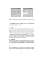
1.1 General
Change the dimension of the algebra to 3 by using the dimension dropdown
box. Change the name of the algebra to e3ga (which stands for euclidean 3
dimensional geometric algebra). This name is arbitrary; you could give a 3d
euclidean algebra any name you like, but in this example we will use e3ga.
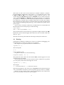
Leave the other properties as is. The window should now look like figure 1a.
a
b
Figure 1: The general and signature tabs with correct settings for the e3ga algebra.
1
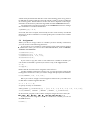
a
b
Figure 2: The products and order tabs with correct settings for the e3ga algebra.
1.2 Signature
Switch to the signature tab. In the signature tab you can change the signature of the algebra. It is shown in figure 1b. Because the default setting is for
an euclidean signature, we don’t have to change anything here. Click on the
products tab.
1.3 Products
A geometric algebra generated by Gaigen does not contain every supported
product by default. Including a product generates more code, which will make
compilation slower and your executable larger. For our example algebra we
would like to have the geometric product, the outer product, the scalar product
and the left contraction (a type of inner product) in our algebra. The geometric
product is included by default. Click on the op tab and tick the checkbox labeled Outer Product. You will see that the tab name will be highlighted in red.
This means that the product is included in the algebra. Repeat the steps above
to also include the scalar (scp) and the left contraction (lcont) in the algebra.
The lower part of the products tab is used to add optimizations to the algebra. Optimized products execute much faster than unoptimized onces, but
they cause more code to be generated. We can’t possibly generate an optimized
version of every possible product for high dimensional algebras (as explained
in the user manual and the paper). That’s why we only want to optimize certain products which are used often.
Suppose we would like to optimize the geometric product of an even versor
and a vector, and of an odd versor and an even versor. Click on the gp tab. Tick
the left 0 and 2 checkboxes (grade parts 0 and 2 are used in an even versor). Tick
the right 1 checkbox (grade part 1 is used in a vector). Click the add button.
The optimization should appear in the list below the checkboxes. Now tick the
left 1 and 3 checkboxes (grade parts 1 and 3 are used in an odd versor). Tick the
right 0 and 2 checkboxes. Click the add button. Another optimization should
appear in the list below the checkboxes. If you do not add the optimizations
correctly, your algebra will still work, but we can’t demonstrate some of the
profiling functionality later on.
2
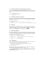
a
b
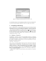
Figure 3: The functions and memory tabs with correct settings for the e3ga
algebra.
Your products tab should now look like figure 2a, with tabs gp, op, lcont
and scp highlighted in red, to signal their inclusion in the algebra, and two
optimizations for the geometric product.
Switch to the order tab.
1.4 Order
The order tab is used to control the order and orientation in which the coordinates are passed to between the generated Gaigen source code and your
application. We wish to change the order and orientation of the grade 2 coordinates, such that they match those of Gable (which is an educational Matlab
package for doing 3d geometric algebra computations). Click on the g.2 tab.
First of all, we want to reverse the orientation of ½ ¿ to ¿ ½ . Click on
the toggle button left of ½ ¿ to accomplish this.
Second, we want the order to be [¾ ¿ , ¿ ½ , ½ ¾ ]. Click on the up
(to move the coordinate up) and down (to move the coordinate down) buttons
until you get this order right. This part of the user interface is awkward, we
know. Your order tab should now look like figure 2b.
1.5 Functions
We would like to include almost all of the available functionality in our algebra
so we can demonstrate and play with them. Besides the default functions,
tick the lounesto inverse, the outer morphism, the factor blade / versor, meet
and join, profile and fast temporary variables checkboxes. Your functions tab
should look like figure 3a.
1.6 Memory
We will use the tight memory allocation algorithm. This algorithm will allocate
exactly the amount of memory required to store the (compressed) coordinates
of our multivectors. Although this might make our (demonstration) program
3
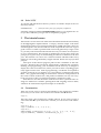
Figure 4: The generate tab with correct settings for the e3ga algebra.
a little bit slower, it can save a lot of memory when you create a lot of multivectors. Floating point variables of type float will be used to store the coordintes
of our multivectors. Figure 3b shows the memory tab with the tight checkbox
ticked.
1.7 Generate
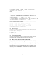
You can switch to the generate tab to have a quick look at it (or take a look
at figure 4). The output dir text field is used to change the directory name
where the generate source will be output. By default, this will be equal to the
name of your algebra. You can also see which files will be generated, in the
upper right part of the tab. The lower part of the tab contents is reserved for
checkboxes which are used to specify what kind of optimized sourcecode will
be generated. By default, the generate c code checkbox is on, but the generate c
’2’ code checkbox is also a good choice. Leave everything the way it is though.
1.8 Saving the algebra specification
You can now save the specification of your e3ga algebra. Click the save algebra button at the bottom right of the window. The save algebra dialog box will
appear. Specify the filename and directory where you want to store the .gas file
and click save. A nice place to save your specifications is in the algebras directory (the algebras directory is set via the configuration file, see the installation
manual). If you copied the sample algebras directory from the package, you
will notice that there already is a file called e3ga.gas in there. This file should
contain specifications which are identical to the ones you just entered, so you
can safely overwrite it if want.
1.9 Generating the source code
The last step is generating the source code for you algebra implementation.
This is done by simply clicking the generate which is always present at the
lower left of the window. By default the source code will be left in a subdirectory called e3ga in the algebras directory. Check the output on the console
4
Figure 5: Adding an include directory in Visual C++ 6.0.
or command prompt to see if everything went OK. You can now terminate the
user interface by pressing the exit button at the lower right of the window.
2 Compiling and linking
Here we explain how to compile the generated source code and the example
tutorial file tut1.cpp into one executable. This step differs on each platform and
compiler, but we try to give more details for Windows / Visual C++ and Unix
/ GCC. The basic procedure is to compile e3ga.cpp, e3ga optc.cpp and tut1.cpp,
and then link these into one executable. The e3ga.cpp and e3ga optc.cpp should
be in the e3ga directory inside your algebra directory. The tut1.cpp file is in the
tut1 directory of the package, together with a makefile (for Unix users) and a
workspace (for Visual C++ 6.0).
2.1 Windows / Visual C++
For Windows / Visual C++ users, we have included a Visual C++ workspace
called tut1.dsw. If you have Visual C++ 6.0 installed you can open this workspace
and compile the program. All you have to do before you compile is make sure
the compiler can find the include file e3ga.h. You can see (at the top of tut1.cpp)
that this file is include as follows:
#include <e3ga/e3ga.h>
Thus we have to add the algebras directory the list of directories where the
compiler searches for header files. The easiest way to do this is to add the
algebras directory to the global list of include directories where the compiler
searches. In Visual C++ click on the tools menu and select options. A dialog
box like the one in figure 5 appears. Click on the directories tab, select include
files from the show directories for dropdown box, and add your algebras directory to the bottom of the list.
After you have added the include directory there should be no problem
compiling.
5
2.2 Unix / GCC
To compile and link the first tutorial, you have to edit the makefile in the tut1
directory. The line
ALGEBRASDIR
= /home/fontijne/ga/gaigen/algebras
should be changed such that ALGEBRASDIR points to your algebras dir. After you have done this, just type make to compile the program.
3 The tutorial source
The tutorial 1 source doesn’t do much more than demonstrate the functionality
of the e3ga algebra implementation. It simply contains sample code which
demonstrates almost every function and feature of e3ga. The idea is that you
read through the code, this text and look at the output at the same time to get a
good overview of what is possible with sourcecode generate by Gaigen. Later
on, you may want to look into the tutorial source if you want to see exactly how
to use a certain feature. The program is divided into several parts, which will
prompt you to press a key or do something else before it continues to the next
part. This tutorial is of course not a reference manual which describes every
feature of sourcecode generated by Gaigen in detail. Please refer to [1] for that
purpose.
Most parts of the tutorial program print out the coordinates of the multivectors. We know that everybody should prefer coordinate-free geometric
thinking and programming , but coordinates are the best way for Gaigen to
display the value of a multivector, unless you want to draw everything graphically right from the start. And in programming, coordinates are required to
get data in and out of your algebra, so it’s important to get familiar with using
them. Also, graphical drawings of multivectors values are interpretations of
the values of those multivectors, and printed coordinates are not; not everybody may agree on how we interpret and draw a multivector value.
Note that we start the discussion with the most basic operations like creating new multivector variables, printing them and assigning values to them,
which are all related to the input and output of coordinates.
3.1 Construction
There are several ways to construct and initialize a new multivector variable.
First of all you can create a new multivector with the value like this:
e3ga a;
This will create a new multivector variable called a. If you want to assign a
value other than to your multivector variable, you can use one of the following:
e3ga b(1.0);
e3ga c(GRADE1, 1.0, 2.0, 0.0);
e3ga d(c);
GAIM_FLOAT coordinates_of_e[4] = {1.0, 2.0, 3.0, 4.0};
e3ga e(GRADE0 | GRADE2, coordinates_of_e);
6
These lines of code create 4 new multivector variables called b, c, d and e.
b is immediately assigned the scalar value 1. c is assigned the vector value
½ ¾ ¿ . If you wanted to assign a bivector value to c, you
would change the GRADE1 parameter to GRADE2. If you wanted a trivector
value, replace GRADE1 by GRADE3 and change the number of coordinates
you specify to 1 instead of 3. The construction of d shows how to construct a
new multivector with the value of another multivector (c in this case). Finally,
the construction of e shows how to construct multivectors with an initialization
value which has multiple grade parts (e.g. a rotor, which has a grade 0 and a
grade 2 part).
If you want to construct a multivector variable which is not allocated from
the stack but from a memory heap, use the following.
e3ga *vptr;
vptr = new e3ga(GRADE3, 1.0);
This would construct a new multivector, pointed to by vptr, with the value .
By the time you have had enough of the multivector, you can delete it like this:
delete vptr;
This frees all memory (allocated from the heap) used by the multivector.
3.2 Printing
Printing the coordinates of multivector can be very useful for debugging, storing them in files, or simply as output of your program.
The simplest way to print the value of a multivector is:
a.print("a: ");
This would print
a: 0
on the standard output.
To print to a file, you can use the following
b.fprint(stdout, "b: ");
This prints the value of b to the file named stdout, which happens to be the
standard output by default.
If you want more control over the format in which a multivector is printed,
you can specify it like in the following line of code:
c.print("c: ", "%e");
This outputs
c: 1.000000e+000*e1 + 2.000000e+000*e2
in the tutorial program. You can use any valid printf format specifier instead of
”%e”. The default, used when you don’t explicitly specify a format, is ”%2.2f”.
Finally you may simply want a string representation of the multivector
value. You can obtain it as shown in this example
7
printf("The value of ’d’ is: %s\nThe value of ’e’ is: %s\n",
d.string(), e.string("%e"));
This line gets the string representation of d and e by calling d.string() and
e.string(”%e”) and then prints these strings using the standard C library function printf.
3.3 Coordinate access
Often it will be necessary to access the coordinates of a multivector, e.g. to
pass them OpenGL to render them, or to write them to a file. This can be
done using the coordinates functions or the [] operator. This is shown in the
following lines of tutorial code:
f1 = b.coordinates(GRADE0)[0];
f2 = b[GRADE0][E3GA_S];
The GRADE macros, which are used as the only argument to the function and
operator, define which grade part of the multivector you want to access. The
function and operator return a pointer to a const (constant) array of floating
point values, thus you can use an index (e.g.[0] or [E3GA S]) to get the value
of a specific coordinates. E3GA S is defined as 0 in e3ga.h. Macros like E3GA S
are defined for every coordinate, so you also write something like this
f1 = e[GRADE2][1];
f2 = e[GRADE2][E3GA_E3_E1];
to access the ¿ ½ coordinate of a multivector variable. Using the E3GA
macros is more portable, since the order in which the coordinates are stored
could be changed (in the order tab of the gaigenui program). When that order
is changer, the value of the E3GA macros is also automatically changed.
There is also a function scalar which simply returns the scalar part of a
multivector:
f3 = b.scalar();
Of course you can temporarily keep a pointer to the coordinates of a grade
part of a multvector, but you must remember that when you change the value
of a multivector, the pointer to the coordinates may become invalid, as this
example demonstrates:
const float *fptr;
fptr = e[GRADE1];
printf("\nThe grade 1 coordinates of ’e’: %2.2f %2.2f %2.2f\n",
fptr[0], fptr[1], fptr[2]);
e.set(GRADE1, 1.0, 2.0, 3.0);
printf("The grade 1 coordinates of ’e’ after the change may"
"be incorrect: %2.2f %2.2f %2.2f\n",
fptr[0], fptr[1], fptr[2]);
The output of the example above could well be
The grade 1 coordinates of ’e’: 0.00 0.00 0.00
The grade 1 coordinates of ’e’ after the change
may be incorrect: 0.00 0.00 0.00
8
which clearly demonstrates that the value of the floating point array point to
by fptr did not change after the call to set, which is used to set the coordinates
of a certain grade. Actual behavior of the code above depends on the implementation of the memory allocation algorithm and the coordinates function.
You should never use the [] operator of the coordinates function to change
the coordinates of a multivector like this:
e[GRADE1][0] = 0.0;
First of all, this won’t compile, and secondly it won’t work correclty. Use the set
function to set the coordinates of a certain grade part of a multivector variable
if you must.
3.4 Assignment
When you ahve to assign values to variables you have already constructed,
you can use one of the following functions.
If you want to set a variable to a homogenous (only grade part not equal to
) multivector value, you can use one of the setX functions, such as setScalar,
setVector and set3Vector:
a.setScalar(1.0);
b.setVector(2.0, 3.0, 4.0);
c.set2Vector(5.0, 6.0, 7.0);
d.set3Vector(8.0);
If you want to copy the value of one multivector variable to another you
can use the overloaded = operator (see section 3.12), or the copy function:
e = b;
e.copy(b);
Both of the the two lines above assign the value of b to e.
Just like with the constructors (section 3.1), you can specify the grade of the
homogenous multivector value you want to assign and specify the coordinates:
b.set(GRADE1, 2.0, 3.0, 4.0);
But if you want to assign a non homogenous multivector you either have
to add other variables together like this:
e = a + b + c + d;
or specify an array of coordinates:
GAIM_FLOAT e_coordinates[8] = {1.0, 2.0, 3.0, 4.0, 5.0, 6.0, 7.0, 8.0};
e.set(GRADE0 | GRADE1 | GRADE2 | GRADE3, e_coordinates);
In the tutorial program, both of these examples assign the same value ( ½ ¾ ¿ ¾ ¿ ¿ ½ ½ ¾ ½ ¾ ¿ ) to e.
If you just want to assign the value to a multivector variable, you can use
the null function:
b.null();
9
Lastly, this example shows how to assign random scalar, blade and versor
values to a multivector variable:
a.randomBlade(GRADE0, 1.0);
b.randomBlade(GRADE2, 1.0);
c.randomVersor(GRADE2, 1.0);
a.print("Random scalar: ");
b.print("Random bivector: ");
c.print("Random versor: ");
This piece of sample code should produce output like the following:
Random scalar: -0.03
Random bivector: -0.09*e2ˆe3 + 0.19*e3ˆe1 + 0.11*e1ˆe2
Random versor: 0.09 + -0.53*e2ˆe3 + -0.30*e3ˆe1 + -0.85*e1ˆe2
3.5 Grade and grade selection
Sometimes you may want to pick one grade part of a multivector variable and
store it in another, e.g. when you know that the other grade parts only contain
(floating point) noise, as in this example:
(c * b / c).print("bivector?: ", "%1.1e");
(c * b / c)(GRADE2).print("bivector: ", "%1.1e");
(c * b / c).grade(GRADE2).print("bivector: ", "%1.1e");
Here, the versor c is applied to the bivector b. We know that the result should
be a bivector again, but due to floating point noise, a scalar element also appears. To get rid of the scalar part, we can use the () operator, or the grade
function. Both return only the requested grade part of the multivector variable, as you can see in the output of the code above:
bivector?: -4.1e-010 + 1.7e-001*e2ˆe3 + -1.5e-001*e3ˆe1 + 7.1e-002*e1ˆe2
bivector: 1.7e-001*e2ˆe3 + -1.5e-001*e3ˆe1 + 7.1e-002*e1ˆe2
bivector: 1.7e-001*e2ˆe3 + -1.5e-001*e3ˆe1 + 7.1e-002*e1ˆe2
The function maxGrade returns the index of the maximum non-zero grade
part of a multivector variable. The function grade (without an argument) returns the grade of a multivector variable if it homogenous, and -1 otherwise.
So this code:
printf("Maximum non-zero grade part of c: %d\n",
c.maxGrade());
printf("The grade of c: %d; the grade of b: %d\n",
c.grade(), b.grade());
would print:
Maximum non-zero grade part of c: 2
The grade of c: -1; the grade of b: 2
10
3.6 Grade involution, clifford conjugate and reverse
The functions gradeInvolution, cliffordConjugate and reverse selectively toggle the sign of some grade parts as you can see in the output of the the sample
code.
a = e.gradeInvolution();
b = e.cliffordConjugate();
c = e.reverse();
3.7 Addition, subtraction, negation
This piece of code generates three random blades in (grade 1), (grade 2)
and (grade 3). It then adds and subtracts them using the add, sub and negate
functions in various ways.
d = add(add(a, b), c);
e = add(d, b.negate()); // subtract ’b’ from ’d’...
e = sub(d, b); // ...which of course is much easier this way
3.8 The dual
The dual function computes the dual of a blade with respect to the pseudoscalar of the algebra. As the code shows, the a blade and it’s dual are orthogonal. Internally, the dual can be computed as ½ , or by using fast
dualization, if the fastDual function is included in the algebra.
3.9 The basic products
Here we demonstrate the use of the basic products such as the geometric product, the left contraction, the outer product and the scalar product. We generate
two random vectors and . Then we compute the product just mentioned
using the gp, lcont, op and scp functions:
c
d
e
a
=
=
=
=
gp(a, b); // geometric product
lcont(a, b); // left contraction (an inner product)
op(a, b); // outer product
scp(a, b); // scalar product
3.10 The inverse
This part of the tutorial first shows the (mis-use) of the various inversion functions, and then goes on to benchmark their performance.
We start with a random grade 2 blade and compute it’s inverse:
a.randomVersor(GRADE2, 1.0);
b = a.inverse();
By the output we can see that this works, except that is not exactly , but
has some very small grade 2 components as well.
The standard inverse function calls the versorInverse function by default.
The versorInverse function works only on versors. When we try to use it on a
general multivector, it fails:
11
e.set(GRADE0 | GRADE1 | GRADE2 | GRADE3, e_coordinates);
(e.inverse() * e).print("1?: ");
output:
1?: 1.00 + 0.44*e1 + 0.44*e2 + 0.62*e3 +
0.00*e2ˆe3 + 0.00*e3ˆe1 + -0.00*e1ˆe2 + -0.00*e1ˆe2ˆe3
When we use the generalInverse and lounestoInverse functions, we see
that they do work for general multivectors:
(e.generalInverse() * e).print("˜ 1: ", "%e");
// ’lounestoInverse’ always works, but is only available in 3d
(e.lounestoInverse() * e).print("˜ 1: ", "%e");
To show why the versor inverse is usefull, we benchmark all there inversion
function. On my machine this results in:
Could do ˜ 629000 versor inverses in 1 second
Could do ˜ 122000 general inverses in 1 second
Could do ˜ 386000 lounesto inverses in 1 second
The versorInverse function is clearly the fastest.
3.11 Meet and join
This section of the tutorial computes the meet (intersection) and join (union) of
two blades using the following code:
c = meet(a, b);
d = join(a, b);
3.12 Overloaded operators
This section demonstrates the use of all overloaded operators. It does not print
out anything, so just read at the code to see what operator does what.
3.13 Basis vectors and the (inverse) pseudoscalar
Here we construct some multivectors using the basis vectors and (inverse)
pseudoscalar that you can access directly:
a = 2.0 * e3ga::e1 + 3.0 * e3ga::e2 + 4.0 * e3ga::e3 + e3ga::I;
b = e3ga::e1 << e3ga::I;
It may sometimes be necessary to cast such a basis vector to type e3ga to avoid
compilation errors as in (e3ga)e3ga::e1, since they are of type e3gai (the internal
class name).
12
3.14 Outermorphism
This piece of tutorial code shows how to use the outer morphism operator.
Currently, the outer morphism operator is quite primitive and can only be initialized by giving it the images of all basis vectors under the linear operation
you want outer morphism to compute. This is done like this in the tutorial
code:
rv[0] = R * e3ga::e1 * Rinv;
rv[1] = R * e3ga::e2 * Rinv;
rv[2] = R * e3ga::e3 * Rinv;
om.initOuterMorphism(rv);
After the outer morphism operator om has been initialized, it can be applied
to a multivector variable like this:
(om * a).print("Rotation using the om: ", "%e");
The nice thing about the outer morphism operator is that it does not produce
grade parts filled with floating point noise like the spinor products does. For
instance
(R * a * Rinv).print("Rotation not using the om: ", "%e");
outputs something like this (note the ½ ¾ ¿ part):
Rotation not using the om: 2.081804e-001*e1 + 5.360851e-001*e2 +
-6.546013e-002* e3 + -1.914059e-008*e1ˆe2ˆe3
while the outer morphism operator outputs something like this:
Rotation using the om: 2.081804e-001*e1 + 5.360851e-001*e2 +
-6.546013e-002*e3
Another advantage is that it is probably faster if you apply it a lot of times
after initializing it, and it can more easily be optimized for using low level
(SSE, 3DNow or altivec) assembler by a (future) opt2X compiler.
3.15 Speedup due to optimizations
If you followed the instructions in section 1.3 correctly, your e3ga algebra is optimized to compute ½ , but not optimized to compute ½ , where
is an even versor and is a vector. This section of the tutorial demonstrates
the performance difference such optimizations might make on your computer.
It computes approximately how many of these spinor products can be computed in 1 second, for each case. The difference is best visible when the profiling function is disabled and fast temporary variables are enabled (these slow
down overall performance, and thus make the difference due to the optimized
spinor product less visible). The optimized version of the spinor product might
be up to four times as fast as the non-optimized version.
If you have a debugger, you can examine the different behavior of the optimized and non-optimized Gaigen code by tracing into the products. You will
see that for the non-optimized products , Gaigen will first unpack the compressed coordinates, then execute a function with a lot of conditional statements (which can stall modern deeply pipelined processors for many cycles),
13
recompress the coordinates and (depending on the memory allocation algorithm) allocate memory to store them. The optimized products on the other
hand immediately know how much memory to allocate, do not have to decompress the coordinates and do not use many conditional jumps.
3.16 Temporary variable allocation
In section 1.5 you turned on fast temporary variables function. Use of fast
temporary variables makes your application faster (as the name suggests), but
it comes at a cost (see [1] for details). If you pass a fast temporary variable
to another function, or keep a reference to it too long, its value might change
unexpectedly. This will cause your application to malfunction. Even worse,
the problem is very hard to debug if you don’t know what you are looking
for. This piece of tutorial code demonstrates the symptons of a fast temporary
variable which has gone bad.
If you have enabled fast temporary variables, the output of the this part of
the tutorial should be something like:
Value before the loop: 1.00
Value after the loop: 0.79 + -0.13*e2ˆe3 + 0.74*e3ˆe1 + 0.86*e1ˆe2
The value in ’referenceToTemporaryVariable’ has changed!
And if you have disabled them, it should output:
Value before the loop: 1.00
Value after the loop: 1.00
The value in ’referenceToTemporaryVariable’ has not changed.
So if you suspect that fast temporary variables are causing a problem in
your program, disable them, regenerate your algebra, and see if the problem
has gone away. If so, search for places where you keep a reference to a temporary variable too long (or simply accept the performance penalty of ’standard
C++ temporary variables’).
References
[1] D. Fontijne. Gaigen user manual.
[2] D. Fontijne, T. Bouma, L. Dorst Gaigen: A Geometric Algebra Implementation
Generator.
14