Download Using a Runtime Measurement Device with Measurement

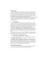
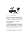
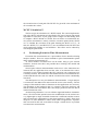
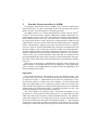
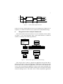
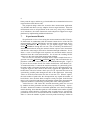
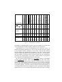
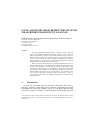
USING A RUNTIME MEASUREMENT DEVICE WITH
MEASUREMENT-BASED WCET ANALYSIS ∗
Bernhard Rieder, Ingomar Wenzel, Klaus Steinhammer, and Peter Puschner
Institut für Technische Informatik
Technische Universität Wien
Treitlstraße 3/182/1
1040 Wien, Austria
[email protected]
Abstract
The tough competition among automotive companies creates a high cost
pressure on the OEMs. Combined with shorter innovation cycles, testing new
safety-critical functions becomes an increasingly difficult issue [4]. In the automotive industry about 55% of breakdowns can be traced back to problems in
electronic systems. About 30% of these incidents are estimated to be caused by
timing problems [7]. It is necessary to develop new approaches for testing the
timing behavior on embedded and real-time systems.
This work describes the integration of runtime measurements using an external measurement device into a framework for measurement-based worst-case
execution time calculations. We show that especially for small platforms using
an external measurement device is a reasonable way to perform execution time
measurements. Such platforms can be identified by the lack of a time source,
limited memory, and the lack of an external interface. The presented device
uses two pins on the target to perform run-time measurements. It works cycle accurate for frequencies up to 200MHz, which should be sufficient for most
embedded devices.
1.
Introduction
Over the last years more and more automotive subsystems have been replaced by electronic control units (ECUs) which are interconnected by high
dependable bus systems like FlexRay, TTP/C or CAN. Much effort has been
put into increasing the reliability of communication and scheduling and great
∗ This work has been supported by the FIT-IT research projects “Automatic Test Data Generation for WCET
Measurements (ATDGEN)” and “Model-based Development of distributed Embedded Control Systems
(MoDECS-d)”.
2
advances in these areas have been made. However, timing analysis, especially
worst-case Execution Time (WCET) analysis of automotive applications, is
still a challenge. This is mainly due to two factors which cumulatively increase complexity of timing analysis: More and more functionality is integrated within single ECUs [4] and the architecture of the processors is getting
more complex, especially by features such as caches, pipelining, branch prediction, out of order execution and others [3]. Additionally, processor vendors
do not offer accurate data sheets describing the features of their processors, so
that those are unknown or have to be figured out by reverse engineering [8].
Without detailed knowledge about processor internals static timing analysis,
that is calculating the time required for the execution of code without actually
executing it, is often not possible.
Therefore, novel approaches use a combination of static analysis and execution time measurements to calculate a WCET bound [10]. The proposed
method consists of static analysis, control flow graph decomposition, test data
generation, execution-time measurement and the final calculation step. All
steps are performed automatically without user interaction. The method is described in Section 3.
Computing resources of embedded applications are often limited and therefore not suitable for runtime measurements. Typical limitations are the lack of
a time source, limited memory (no location to store measurement data), and the
lack of an external interface (no way to transfer measurement data to host). As
a solution we developed an external measurement device, which is based on an
FPGA and therefore very flexible and inexpensive. We demonstrate the usage
of the execution time measurement device by performing WCET calculations
using a HSC12 microcontroller evaluation board. The proposed solution uses
only a single instruction per measurement point and two pins for the interface
to the measurement device.
Structure of this Article
This paper is structured as follows: In Section 2 we present related work in
the domain of dynamic WCET estimation and execution time measurement.
The measurement-based WCET analysis approach is described in Section 3.
Section 4 outlines basic requirements when performing execution time measurements for timing analysis. In Section 5 we describe the hardware and
firmware design of the measurement device. Section 6 explains how execution
time measurements are performed by the timing analysis framework. The conducted experiments are described in Section 7. At last, Section 8 gives a short
conclusion and an overview of open topics.
3
Contributions
The first contribution is the introduction of a dedicated runtime measurement device (RMD). The device works for CPU frequencies of up to 200 MHz.
It is linked to the target using a simple 2-wire connection. Since the device is
built using a field programmable gate array (FPGA) it can easily be extended
or reconfigured and is very flexible. The device is especially useful to perform
execution time measurements on targets with limited resources.
Second, the device is seamlessly integrated into an novel developed measurementbased WCET calculation framework as described in [10]. All operations of
the measurement-based WCET analysis are performed fully automatic without user interaction.
2.
Related Work
Petters [5] describes a method to split an application down to “measurement blocks” and to enforce execution paths by replacing conditional jumps
either by NOPs or unconditional jumps, eliminating the need for test data. The
drawback is that the application is partitioned manually and that the measured,
semantically changed application may differ from the real application.
Bernat et al. introduce the term of a “probabilistic hard real-time system”.
They combine a segmented measurement approach and static analysis, however they use test data supplied by the user. Therefore they cannot guarantee a
WCET bound but only give a probabilistic estimation, based on the used test
data [1].
Petters describes various ways to collect execution traces of applications in
[6]. He outlines various ways how to place “observation points” and discusses
benefits and drawbacks of the presented methods.
3.
Measurement-Based WCET Analysis
The proposed measurement-based timing analysis (MBTA) is performed in
five steps [9] as shown in Figure 1
The individual steps are explicitly described below. The measurement device hardware is used in step ➃ but the description of the other steps is necessary to understand how the MBTA approach works. It is also important to
mention that the current implementation is limited to acyclic code (code without loops). Since most modeling tools typically produce acyclic code this does
not strongly limit the applicability of the presented method.
Static Program Analysis ➀
This step is used to extract structural and semantic information from the C
source code. The information is needed to perform the next steps.
4
Figure 1.
MBTA Framework Overview
Control Flow Graph Decomposition ➁
During this phase, the control flow graph CFG of the analyzed program is
split up into smaller program segments PS. The subdivision is controlled by
the number of execution paths which remain within each PS, a number which
is denoted as path bound. The command line argument for the path bound
is adjustable from 1 to 232 and controls the correlation between calculation
time and the number of required measurements: A high path bound causes a
lower number of PS and less measurement points but the sum of execution
paths through all PS increases. Since each execution path of each PS has to be
measured, a test data set is required for each path. Since test data calculation
is very time consuming, the calculation time rises significantly [11].
Test Data Generation ➂
In this step test data is calculated to execute all execution paths of each PS.
The test data is acquired using a multi-stage process: Random search which
is very fast is used to find most data sets. Where random search fails, model
checking is used. Model checking is exhaustive, that means if there exists a
data set to execute a certain path, then it will be found. If no data can be found
for a particular execution path then the path is semantically infeasible. An
example for semantically infeasible paths are mutual exclusive conditions in
consecutive if statements. We used the CBMC model checker [2], which is a
very fast bounded model checker that can directly process C input.
Execution Time Measurements ➃
Using the generated test data all feasible paths within each PS are executed.
The result of this step is an execution time profile for each PS which includes
5
the execution time of each path. The WCET of a given PS is the maximum of
all execution time values.
WCET Calculation ➄
The last step is the calculation of a WCET bound. The current implementation of the WCET calculation tool described in [10] uses a longest path search
algorithm for a directed, acyclic graph which a single start and ending node
to compute a WCET bound over all PS. This can lead to overestimations under certain circumstances, namely when the execution path with the WCET
of P Sx inhibits the execution of the path featuring the WCET of P Sy . In
this case WCET(P Sx) and WCET(P Sy ) are accumulated in the WCET of the
whole application leading to overestimation. This effect can be reduced by
increasing the path bound.
4.
Performing Execution Time Measurements
Execution time measurements are a precondition for the described timing
analysis method. There are various methods to place instrumentation points
and to perform measurements [6].
As a first method, execution traces can be made, using a cycle accurate
simulator. In most cases this is not possible due to missing CPU models and
documentation.
Second, pure software instrumentation can be used: A few instructions are
inserted into the application that read the value of an internal time source,
commonly a cycle counter located in the CPU, and write it to a output port or to
a memory location. The drawback of this method is that several instructions are
needed and therefore the code size and the execution time can be considerably
increased.
The third option is to use pure hardware instrumentation. A logic analyzer
is connected to the address bus and records the access to the memory. The advantage of this method is that no alterations on the applications are necessary.
The drawback of this method is that it is expensive (the logic analyzer) and
that the connection to the address bus is not always possible or the CPU has an
internal instruction cache.
An interesting alternative is to use software supported hardware instrumentation. We selected this option because the modifications on the software are
very lightweight (a single assembler instruction is sufficient) and the resource
and execution time consumption on the target hardware is small. Since logic
analyzers are often difficult to control from within an application, expensive
and oversized for this task we decided to design a custom device to perform
execution time measurements.
6
5.
Runtime Measurement Device (RMD)
The Runtime Measurement Device (RMD) acts as interface between the
target and the host. It collects timestamps issued from the target and transfers
them to the host. The timestamps are internally generated.
R
The RMD consists of a custom designed FPGA board with an Altera
TM
Cyclone EP1C12C6 device which is additionally equipped with 64k of external memory (for the CPU core) and interface circuits for USB, Ethernet,
RS232, RS485, ISO-K, and CAN. A modern FPGA evaluation board can also
be used instead, however with a total price of approximately e 300.00 (with
USB interface only) the custom made board is cheaper than most evaluation
R
boards. The firmware is split up in two parts. The first part runs on a NIOS
CPU core which is clocked with 50MHz and controls the communication with
the host computer. The second part is written in VHDL (Very High Speed Integrated Circuit Hardware Description Language) and operates at a clock frequency of 200MHz. This part contains the time base, which is a 32 bit counter,
a FIFO to store up to 128 measurement values until they are transfered to the
host and additional glue logic which recognizes measurement points and stores
the actual counter value in the FIFO and synchronizes communication with the
CPU core.
Since most of the design is implemented within the FPGA firmware the
whole method is very flexible and can easily be adopted for custom application
needs. Changes in the configuration can simply be made by uploading a new
firmware design on the FPGA.
Operation
The measurement device is designed to work in two different modes. The
first mode, the 2-wire mode, uses two dedicated IO pins for the measurements
as depicted in Figure 2. Measurement starts when one signal drops to low.
The internal counter is released and starts counting. On each measurement
point, one signal drops to low, causing the counter value to be stored in the
FIFO, and the other signal rises to high. If both signals are low for a adjustable
amount of time, the measurement stops. According to the FIFO size up to 128
measurement points can be recorded on a single run.
The second mode is the analyzer mode. This mode is designed for very
small devices. In this mode the measurement device is connected to the CPU
address bus and records the time at certain predefined locations. The addresses
where time tamps have to be recorded are stored in a one bit wide RAM. Measurements are taken when the output of the RAM is logical “1”. The advantage
of this mode is that there need be no alterations on the target code. The disadvantages are that knowledge about the physical location of the measurement
7
timeout
1
Pin1
0
1
Pin2
0
time
Start
T1
T2
Figure 2.
Stop
2-Wire Interface Signal Waveform
points is necessary and that physical access to the address bus of the device is
required, so it cannot be used for devices with on-board E(E)PROM storage.
6.
Integration in the Analysis Framework
The measurement framework consists of a set of virtual base classes shown
in Figure 3. For each virtual base class a non-virtual subclass is loaded at
runtime, according to the underlying hardware.
compile
+prepareCompile(string fname)()
+make()()
+getBinaryName()() : string
+removeFiles()()
+cleanup()()
+getVersion()()
Compile_HCS12
counter
+prepareCounter()()
+readResult()() : long
+close()()
CounterDevice_HCS12Internal
CounterDevice_HCS12External
loader
target
+load(string binary name)()
+wait_for_target_ready()()
+start_program()()
+reset_target()()
Loader_HCS12
Target_HCS12
Figure 3.
Measurement Application Class Framework [9]
The compile class is used to compile the application on the host and to
generate a stub for the target to handle the communication with the host, load
the test data, and to execute the application. The counter class activates the
source code for starting and stopping the counter on the target and handles the
communication between the host and the counting device for both, internal and
external counting devices. The loader class is used to upload the application
8
binary onto the target, and the target class handles the communication between
target and host from the host side.
The proposed design makes the execution time measurement application
very flexible and allows an easy adoption for new target hardware. Since the
measurement runs are all performed in the same way, using only a different
set of subclasses, the whole framework can be adopted to support new target
platforms by implementing additional subclasses.
7.
Experimental Results
We performed a series of tests using the measurement-based WCET analysis framework in combination with the internal counter device of the HCS12
microcontroller (HCS12 INTERNAL) and the runtime measurement device
(HCS12 EXTERNAL). As expected, we got slightly bigger values using
HCS12 INTERNAL during first test runs. This is caused by the different instrumentation methods (using the internal counter requires more instructions
and therefore takes longer) and can be eliminated through calibration. To calibrate, a series of zero-length code sequences are measured and the result is
subtracted from the actual measurements. For all tests the resulting WCET
values were the same using both measurement methods.
The test cases we used were developed from a simple example from our regression tests (nice partitioning semantisch richtig) and from automotive applications (ADCKonv, AktuatorSysCtrl, and AktuatorMotorregler). Figure 4
[9] shows the test results for all case studies for different “Path Bounds (b)”.
As mentioned before, b controls the maximum number of syntactically possible paths within a Program Segment (PS) after the CFG decomposition step.
“Program Segments (PS)” shows in how many segments the Application was
broken down. The next column “Paths After Dec.➁” represents the sum of all
syntactically possible paths through each PSs of the application. Interesting
values are at the first and on the last line of each test case. When b equals 1
the total number of paths after the decomposition step equals the number of
basic blocks, since one basic block comprises exactly one path. In the last line
there is only a single PS and therefore the number of paths after decomposition
equals the number of syntactically possible paths of the whole application.
“Paths Heuristic” and “Paths MC” describe how many paths were covered
by random test data generation and how many by model checking. “Infeasible Paths” denotes the number of infeasible paths that were discovered during
model checking. Note that these paths are also included in the number of paths
covered by model checking. Infeasible paths are paths that are syntactically
possible but can never be executed because the semantics of the code does not
allow so. Since the number of paths covered by model checking is similar to
ADCKonv
(321 LOC)
AktuatorSysCtrl
(274 LOC)
AktuatorMotorregler (1150
LOC)
Figure 4.
6 24
0 151
34
4 10
0 151
15
3 11
0 151
16
2 16
3 150
22
1 71 46 129 106
31
0
0 872
24
8
9
8 870
31
8 66 60 872 220
12 132 132 872 483
54
0
0 173
26
36
0
0 173
10
18 79 72 131 191
165
6
6 n.a. 468
63 29 23 3445 841
57 279 247 3323 7732
82 1373 1325 3298 41353
Paths / PS
Time ETM / Path [s]
Time MC / Path [s]
Overall Time [s]
Time ETM [s]
Time MC [s]
WCET Bound [cyc]
30
14
14
18
72
31
17
74
144
54
36
97
171
92
336
1455
Infeasible Paths
30
6
3
2
1
31
3
2
1
54
14
1
171
14
7
5
Paths MC
1
5
10
20
100
1
10
100
1000
1
10
100
1
10
100
1000
Paths Heuristic
Paths After Dec. ➁
nice partitioning
semantisch richtig
(46 LOC)
Program Segments (PS)
Application Name
Path Bound (b)
9
175 209 1.42 5.8 1.0
39
54 1.50 2.8 2.3
21
37 1.45 1.5 4.7
16
38 1.38 1.1 9.0
12 118 1.49 0.5 72.0
192 216 n.a. 6.2 1.0
22
53 3.44 2.4 5.7
17 237 3.33 1.2 37.0
11 494 3.66 0.9 144.0
318 344 n.a. 5.9 1.0
85
95 n.a. 2.4 2.6
10 201 2.42 0.4 97.0
1289 1757 78.0 7.8 1.0
116 957 29.0 1.7 6.6
62 7794 27.7 0.7 48.0
49 41402 30.1 0.4 291.0
Test Results Of Case Studies
the number of infeasible paths (except for the first example) we see that most
of the feasible paths could be found by random test data generation.
“WCET Bound [cyc]” gives the estimated WCET in processor cycles. To
identify performance bottlenecks we did not only measure the time required
for the complete WCET estimation (“Overall Time”) but also how much of
this time budget was consumed by the analysis (“Time MC”), which consists
mainly of model checking but also includes static analysis, CFG decomposition and random test data generation, and how much time was consumed by
execution time measurements (“Time ETM”), which consists of code generation, compilation and uploading the binary to the target.
We also observed the performance of our solution relative to the number
imeM C
of paths, where “Time MC / Path” equals PT athsM
C and ‘Time ETM / Path”
T imeET M
equals f easibleP aths . While the time required for model checking a single path
within a PS is approximately constant for each test case, the time required for
the execution time measurement of an individual path drops with the number
of program segments. This is due to the fact that the current implementation is
very simple and measures only a single PS at a time. To measure another PS the
application needs to be recompiled and uploaded to the target again. On bigger
10
applications higher values for b should be used so the time fraction required
for recompilation and uploading is much less than for a given examples. The
last column (“Paths / PS”) shows the average number of syntactically possible
paths through a PS.
Regarding the path bound b it can also be noted that the quality of the estimated WCET bound improves with a rising path bound. This is caused by the
fact that semantically infeasible paths are only detected by the model checker
when they are located within the same PS. Therefore, the bigger the PSs the
more infeasible paths can be eliminated.
The fact that the longest measurement runs took little more than 11 hours
(for current industrial code) is very promising. Generating test data sets and
performing the necessary measurements manually for an application of this
size would take a few days at least. We think that this approach can significantly improve the testing process. It should also be noted that test data are
stored and reused for later runs. For applications featuring many infeasible
paths we are currently working on a solution to identify groups of infeasible
paths in a single run of the model checker.
With the case study “AktuatorMotorregler” we reached the computational
limit of the model checker when we set b to 1 therefore we could not get an
WCET estimation value in this case.
8.
Conclusion and Further Work
We found that the measurement-based WCET analysis approach in combination with the presented device gives the application developer a powerful
tool to perform WCET analysis. The most powerful feature is that everything
is performed automatically. This saves valuable working time and eliminates
cumbersome tasks like test data generation and performing manual measurements. The newly introduced measurement device makes it possible to perform
run time measurements on small devices which normally would lack the appropriate hardware support (time source, memory or interface). The measurement
device is cheap - and since it is based on a programmable logic device - very
flexible, which allows the adaption for other hardware devices if necessary.
An important drawback is that, depending on the used RMD-target interface, at least two signal pins are required to perform measurements. Therefore
the measurement device cannot be used when less than two pins are free.
The next step is to overcome limitations of the current measurement framework: loops and functions are not supported in the prototype. We are confident
that these are only limitations of the current design of the prototype and of the
measurement method itself. Currently a new version of the prototype which
supports loops and function calls is in development.
11
The test data generation by model checking can be boosted by cutting off
infeasible subtrees in the dominator tree. If a node cannot be reached then
all other nodes dominated by it are unreachable as well. However the current
implementation makes no use of this information and checks each leaf in the
dominator tree which represents an unique path within a program segment.
An interesting area for improvement is the reconfiguration the RMD firmware
from within the framework for different types of target hardware.
Additionally we are working on a solution to make the measurement-based
approach work on more complex architectures, as those are increasingly used
in new embedded solutions. The presence of caches, pipelines and out-of-order
execution units impose an internal state on the processor. Different hardware
states at the same instruction can result in different execution times. Therefore
we are searching ways to impose a well defined hardware state while loosing a
minimum on performance.
References
[1] G. Bernat, A. Colin, and S. M. Petters. WCET Analysis of Probabilistic Hard Real-Time
Systems. RTSS, 00:279, 2002.
[2] E. Clarke and D. Kroening. ANSI-C Bounded Model Checker User Manual. August 2
2006.
[3] R. Heckmann, M. Langenbach, S. Thesing, and R. Wilhelm. The influence of processor
architecture on the design and the results of WCET tools. Proceedings of the IEEE,
91(7):1038–1054, 2003.
[4] H. Heinecke, K. Schnelle, H. Fennel, J. Bortolazzi, L. Lundh, J. Leflour, J. Maté,
K. Nishikawa, and T. Scharnhorst. AUTomotive Open System ARchitecture-An IndustryWide Initiative to Manage the Complexity of Emerging Automotive E/E Architectures.
Proc. Convergence, SAE-2004-21-0042, 2004.
[5] S. Petters. Bounding the execution time of real-time tasks on modern processors. RealTime Computing Systems and Applications, 2000. Proceedings. Seventh International
Conference on, pages 498–502, 2000.
[6] S. M. Petters. Comparison of trace generation methods for measurement based WCET
analysis. In 3nd Intl. Workshop on Worst Case Execution Time Analysis, Porto, Portugal, July 1 2003. Satellite Workshop of the 15th Euromicro Conference on Real-Time
Systems.
[7] Rapita Systems. Rapitime whitepaper. 2005.
[8] C. Thomborson and Y. Yu. MEASURING DATA CACHE AND TLB PARAMETERS
UNDER LINUX. Proceedings of the 2000 Symposium on Performance Evaluation of
Computer and Telecommunication Systems, pages 383–390, 2000.
[9] I. Wenzel. Measurement-Based Timing Analysis of Superscalar Processors. PhD thesis, Technische Universität Wien, Institut für Technische Informatik, Treitlstr. 3/3/182-1,
1040 Vienna, Austria, 2006.
[10] I. Wenzel, R. Kirner, B. Rieder, and P. Puschner. Measurement-based worst-case execution time analysis. Software Technologies for Future Embedded and Ubiquitous Systems,
2005. SEUS 2005. Third IEEE Workshop on, pages 7–10, 2005.
[11] I. Wenzel, B. Rieder, R. Kirner, and P. Puschner. Automatic timing model generation by
cfg partitioning and model checking. In Proc. Conference on Design, Automation, and
Test in Europe, Mar. 2005.