Download RODIN Deliverable D30

Project IST-511599
RODIN
“Rigorous Open Development Environment for Complex Systems”
RODIN Deliverable 3.6 (D30)
Public Versions of Basic Tools and
Platform
Editor: Laurent Voisin (ETH Zurich)
Public Document
October 29, 2007
http://rodin.cs.ncl.ac.uk
Contributors:
Jean-Raymond Abrial (ETH Zurich)
Stefan Hallerstede (ETH Zurich)
Thai Son Hoang (ETH Zurich)
Gabriel Katz (ETH Zurich)
Farhad Mehta (ETH Zurich)
Christophe Métayer (ClearSy)
François Terrier (ETH Zurich)
Laurent Voisin (ETH Zurich)
Foreword
This deliverable groups together four documents providing support for the
users of the RODIN platform:
1. User Manual of the RODIN Platform
2. The Event-B Modelling Notation
3. The Event-B Mathematical Language
4. Tutorials for RODIN
All these documents, as well as the platform itself, are available from the
SourceForge web site of the Rodin platform
http://rodin-b-sharp.sourceforge.net .
User Manual of the RODIN Platform
October 2007
Version 2.3
User Manual of the RODIN Platform
Contents
1
2
Project
1
1.1
Project Constituents and Relationships . . . . . . . . . . . . . . . . . . . . . . . . . . .
1
1.2
The Project Explorer . . . . . . . . . . . . . . . . . . . . . . . . . . . . . . . . . . . .
2
1.3
Creating a Project . . . . . . . . . . . . . . . . . . . . . . . . . . . . . . . . . . . . . .
3
1.4
Removing a Project . . . . . . . . . . . . . . . . . . . . . . . . . . . . . . . . . . . . .
4
1.5
Exporting a Project . . . . . . . . . . . . . . . . . . . . . . . . . . . . . . . . . . . . .
4
1.6
Importing a Project . . . . . . . . . . . . . . . . . . . . . . . . . . . . . . . . . . . . .
5
1.7
Changing the Name of a Project . . . . . . . . . . . . . . . . . . . . . . . . . . . . . .
5
1.8
Creating a Component . . . . . . . . . . . . . . . . . . . . . . . . . . . . . . . . . . .
5
1.9
Removing a Component . . . . . . . . . . . . . . . . . . . . . . . . . . . . . . . . . .
6
Anatomy of a Context
6
2.1
Carrier Sets . . . . . . . . . . . . . . . . . . . . . . . . . . . . . . . . . . . . . . . . .
8
2.1.1
Carrier Sets Creation Wizard. . . . . . . . . . . . . . . . . . . . . . . . . . . .
8
2.1.2
Direct Editing of Carrier Sets. . . . . . . . . . . . . . . . . . . . . . . . . . . .
8
2.2
Enumerated Sets . . . . . . . . . . . . . . . . . . . . . . . . . . . . . . . . . . . . . .
9
2.3
Constants . . . . . . . . . . . . . . . . . . . . . . . . . . . . . . . . . . . . . . . . . .
10
2.3.1
Constants Creation Wizard. . . . . . . . . . . . . . . . . . . . . . . . . . . . .
10
2.3.2
Direct Editing of Constants. . . . . . . . . . . . . . . . . . . . . . . . . . . . .
11
Axioms . . . . . . . . . . . . . . . . . . . . . . . . . . . . . . . . . . . . . . . . . . .
12
2.4.1
Axioms Creation Wizard. . . . . . . . . . . . . . . . . . . . . . . . . . . . . .
12
2.4.2
Direct Editing of Axioms. . . . . . . . . . . . . . . . . . . . . . . . . . . . . .
12
Theorems . . . . . . . . . . . . . . . . . . . . . . . . . . . . . . . . . . . . . . . . . .
13
2.5.1
Theorems Creation Wizard. . . . . . . . . . . . . . . . . . . . . . . . . . . . .
13
2.5.2
Direct Editing of Theorems. . . . . . . . . . . . . . . . . . . . . . . . . . . . .
14
2.6
Adding Comments . . . . . . . . . . . . . . . . . . . . . . . . . . . . . . . . . . . . .
15
2.7
Dependencies . . . . . . . . . . . . . . . . . . . . . . . . . . . . . . . . . . . . . . . .
15
2.8
Pretty Print . . . . . . . . . . . . . . . . . . . . . . . . . . . . . . . . . . . . . . . . .
16
2.4
2.5
i
3
Anatomy of a Machine
17
3.1
Dependencies . . . . . . . . . . . . . . . . . . . . . . . . . . . . . . . . . . . . . . . .
17
3.2
Variables . . . . . . . . . . . . . . . . . . . . . . . . . . . . . . . . . . . . . . . . . .
18
3.2.1
Variables Creation Wizard. . . . . . . . . . . . . . . . . . . . . . . . . . . . . .
18
3.2.2
Direct Editing of Variables. . . . . . . . . . . . . . . . . . . . . . . . . . . . . .
18
Invariants . . . . . . . . . . . . . . . . . . . . . . . . . . . . . . . . . . . . . . . . . .
19
3.3.1
Invariants Creation Wizard. . . . . . . . . . . . . . . . . . . . . . . . . . . . .
19
3.3.2
Direct Editing of Invariants. . . . . . . . . . . . . . . . . . . . . . . . . . . . .
20
Theorems . . . . . . . . . . . . . . . . . . . . . . . . . . . . . . . . . . . . . . . . . .
20
3.4.1
Theorems Creation Wizard. . . . . . . . . . . . . . . . . . . . . . . . . . . . .
20
3.4.2
Direct Editing of Theorems. . . . . . . . . . . . . . . . . . . . . . . . . . . . .
21
Events . . . . . . . . . . . . . . . . . . . . . . . . . . . . . . . . . . . . . . . . . . . .
21
3.5.1
Events Creation Wizard. . . . . . . . . . . . . . . . . . . . . . . . . . . . . . .
21
3.5.2
Direct Editing of Events. . . . . . . . . . . . . . . . . . . . . . . . . . . . . . .
22
3.6
Adding Comments . . . . . . . . . . . . . . . . . . . . . . . . . . . . . . . . . . . . .
24
3.7
Pretty Print . . . . . . . . . . . . . . . . . . . . . . . . . . . . . . . . . . . . . . . . .
24
3.8
Dependencies: Refining a Machine . . . . . . . . . . . . . . . . . . . . . . . . . . . . .
25
3.9
Adding more Dependencies . . . . . . . . . . . . . . . . . . . . . . . . . . . . . . . . .
25
3.9.1
Abstract Event . . . . . . . . . . . . . . . . . . . . . . . . . . . . . . . . . . .
25
3.9.2
Splitting an Event . . . . . . . . . . . . . . . . . . . . . . . . . . . . . . . . . .
26
3.9.3
Merging Events . . . . . . . . . . . . . . . . . . . . . . . . . . . . . . . . . . .
26
3.9.4
Witnesses . . . . . . . . . . . . . . . . . . . . . . . . . . . . . . . . . . . . . .
26
3.9.5
Variant . . . . . . . . . . . . . . . . . . . . . . . . . . . . . . . . . . . . . . .
27
3.3
3.4
3.5
4
Saving a Context or a Machine
28
4.1
Automatic Tool Invocations . . . . . . . . . . . . . . . . . . . . . . . . . . . . . . . . .
28
4.2
Errors. The Problems Window . . . . . . . . . . . . . . . . . . . . . . . . . . . . . . .
29
4.3
Preferences for the Auto-prover . . . . . . . . . . . . . . . . . . . . . . . . . . . . . .
30
5
The Proof Obligation Explorer
31
6
The Proving Perspective
34
6.1
Loading a Proof . . . . . . . . . . . . . . . . . . . . . . . . . . . . . . . . . . . . . . .
34
6.2
The Proof Tree . . . . . . . . . . . . . . . . . . . . . . . . . . . . . . . . . . . . . . .
34
6.2.1
34
Description of the Proof Tree . . . . . . . . . . . . . . . . . . . . . . . . . . . .
ii
6.2.2
Decoration . . . . . . . . . . . . . . . . . . . . . . . . . . . . . . . . . . . . .
35
6.2.3
Navigation within the Proof Tree . . . . . . . . . . . . . . . . . . . . . . . . . .
35
6.2.4
Hiding . . . . . . . . . . . . . . . . . . . . . . . . . . . . . . . . . . . . . . .
36
6.2.5
Pruning . . . . . . . . . . . . . . . . . . . . . . . . . . . . . . . . . . . . . . .
36
6.2.6
Copy/Paste . . . . . . . . . . . . . . . . . . . . . . . . . . . . . . . . . . . . .
36
6.3
Goal and Selected Hypotheses . . . . . . . . . . . . . . . . . . . . . . . . . . . . . . .
37
6.4
The Proof Control Window . . . . . . . . . . . . . . . . . . . . . . . . . . . . . . . . .
38
6.5
The Smiley . . . . . . . . . . . . . . . . . . . . . . . . . . . . . . . . . . . . . . . . .
40
6.6
The Operator ”Buttons” . . . . . . . . . . . . . . . . . . . . . . . . . . . . . . . . . . .
40
6.7
The Search Hypotheses Window . . . . . . . . . . . . . . . . . . . . . . . . . . . . . .
40
6.8
The Automatic Post-tactic . . . . . . . . . . . . . . . . . . . . . . . . . . . . . . . . .
41
6.8.1
Rewrite rules . . . . . . . . . . . . . . . . . . . . . . . . . . . . . . . . . . . .
41
6.8.2
Automatic inference rules . . . . . . . . . . . . . . . . . . . . . . . . . . . . .
47
6.8.3
Preferences for the Post-tactic . . . . . . . . . . . . . . . . . . . . . . . . . . .
50
Interactive Tactics . . . . . . . . . . . . . . . . . . . . . . . . . . . . . . . . . . . . . .
50
6.9.1
Interactive Rewrite Rules . . . . . . . . . . . . . . . . . . . . . . . . . . . . . .
50
6.9.2
Interactive Inference rules . . . . . . . . . . . . . . . . . . . . . . . . . . . . .
56
6.9
A The Mathematical Language
60
B ASCII Representations of the Mathematical Symbols
60
B.1 Atomic Symbols . . . . . . . . . . . . . . . . . . . . . . . . . . . . . . . . . . . . . .
61
B.2 Unary Operators . . . . . . . . . . . . . . . . . . . . . . . . . . . . . . . . . . . . . . .
61
B.3 Assignment Operators . . . . . . . . . . . . . . . . . . . . . . . . . . . . . . . . . . .
61
B.4 Binary Operators . . . . . . . . . . . . . . . . . . . . . . . . . . . . . . . . . . . . . .
62
B.5 Quantifiers . . . . . . . . . . . . . . . . . . . . . . . . . . . . . . . . . . . . . . . . . .
63
B.6 Bracketing . . . . . . . . . . . . . . . . . . . . . . . . . . . . . . . . . . . . . . . . . .
63
iii
Foreword
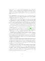
The reader of this Manual is supposed to have a basic acquaintance with Eclipse. Basic help about using
the Eclipse platform is available on-line from the RODIN platform. To view it, select Help > Help
Contents from the menubar. Then, select Workbench User Guide in the Web browser window that pops
up.
1
1.1
Project
Project Constituents and Relationships
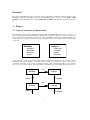
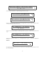
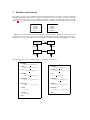
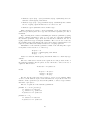
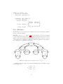
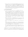
The primary concept in doing formal developments with the RODIN Platform is that of a project. A
project contains the complete mathematical development of a Discrete Transition System. It is made of
several components of two kinds: machines and contexts. Machines contain the variables, invariants, theorems, and events of a project, whereas contexts contain the carrier sets, constants, axioms, and theorems
of a project:
Context
Machine
carrier sets
constants
axioms
theorems
variables
invariants
theorems
events
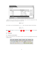
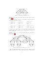
We remind the reader of the various relationships existing between machines and contexts. This is
illustrated in the following figure. A machine can be ”refined” by another one, and a context can be
”extended” by another one (no cycles are allowed in either of these relationships). Moreover, a machine
can ”see” one or several contexts. A typical example of machine and context relationship is shown below:
sees
Context
Machine
extends
refines
sees
Context
Machine
refines
extends
1
1.2
The Project Explorer
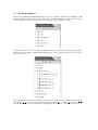
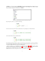
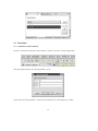
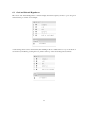
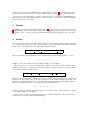
Projects are reachable in the RODIN platform by means of a window called the ”Project Explorer”. This
window is usually situated on the left hand side of the screen (but, in Eclipse, the place of such windows
can be changed very easily). Next is a screen shot showing a ”Project Explorer” window:
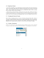
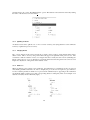
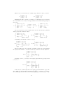
As can be seen in this screen shot, the Project Explorer window contains the list of current project names.
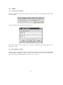
Next to each project name is a little triangle. By pressing it, one can expand a project and see its components as shown below.
We expanded the project named ”celebrity”. This project contains 2 contexts named ”celebrity ctx 0”
and ”celebrity ctx 1”. It also contains 4 machines named ”celebrity 0” to ”celebrity 3”. The icons ((c) or
(m)) situated next to the components help recognizing their kind (context or machine respectively)
2
In the remaining parts of this section we are going to see how to create (section 1.3), remove (section
1.4), export (section 1.5), import (section 1.6), change the name (section 1.7) of a project, create a component (section 1.8), and remove a component (section 1.9). In the next two sections (2 and 3) we shall
see how to manage contexts and machines.
1.3
Creating a Project
In order to create a new project, simply press the button as indicated below in the ”Project Explorer”
window:
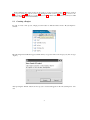
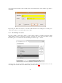
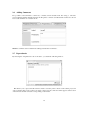
The following wizard will then appear, within which you type the name of the new project (here we type
”alpha”):
After pressing the ”Finish” button, the new project is created and appears in the ”Project Explorer” window.
3
1.4
Removing a Project
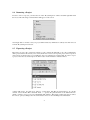
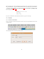
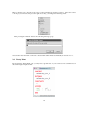
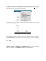
In order to remove a project, you first select it on the ”Project Explorer” window and then right click with
the mouse. The following contextual menu will appear on the screen:
You simply click on ”Delete” and your project will be deleted (confirmation is asked). It is then removed
from the Project Explorer window.
1.5
Exporting a Project
Exporting a project is the operation by which you can construct automatically a ”zip” file containing the
entire project. Such a file is ready to be sent by mail. Once received, an exported project can be imported
(next section), it then becomes a project like the other ones which were created locally. In order to export
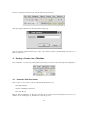
a project, first select it, and then press the ”File” button in the menubar as indicated below:
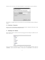
A menu will appear. You then press ”Export” on this menu. The Export wizard will pop up. In this
window, select ”Archive File” and click ”Next >”. Specify the path and name of the archive file into
which you want to export your project and finally click ”Finish”. This menu sequence belongs (as well as
the various options) to Eclipse. For more information, have a look at the Eclipse documentation.
4
1.6
Importing a Project
A ”.zip” file corresponding to a project which has been exported elsewhere can be imported locally. In
order to do that, click the ”File” button in the menubar (as done in the previous section). You then click
”Import” in the coming menu. In the import wizard, select ”Existing Projects into Workspace” and click
”Next >”. Then, enter the file name of the imported project and finally click ”Finish”. Like for exporting,
the menu sequence and layout are part of Eclipse.
The importation is refused if the name of the imported project (not the name of the file), is the same as
the name of an existing local project. The moral of the story is that when exporting a project to a partner
you better modify its name in case your partner has already got a project with that same name (maybe a
previous version of the exported project). Changing the name of a project is explained in the next section.
1.7
Changing the Name of a Project
The procedure for changing the name of a project is a bit heavy at the present time. Here is what you
have to do. Select the project whose name you want to modify. Enter the Eclipse ”Resource” perspective.
A ”Navigator” window will appear in which the project names are listed (and your project still selected).
Right click with the mouse and, in the coming menu, click ”Rename”. Modify the name and press enter.
Return then to the original perspective. The name of your project has been modified accordingly.
1.8
Creating a Component
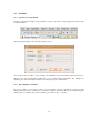
In this section, we learn how to create a component (context or machine). In order to create a component
in a project, you have to first select the project and then click the corresponding button as shown below:
5
You may now choose the type of the component (machine or context) and give it a name as indicated:
Click ”Finish” to eventually create the component. The new component will appear in the Project Explorer
window.
1.9
Removing a Component
In order to remove a component, press the right mouse button. In the coming menu, click ”Delete”. This
component is removed from the Project Explorer window.
2
Anatomy of a Context
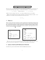
Once a context is created, a window such as the following appears in the editing area (usually next to the
center of the screen):
You are in the ”Edit” area allowing you to edit pieces of the context, namely dependencies (keyword
”EXTENDS”), carrier sets (keyword ”SETS”), constants (keyword ”CONSTANTS”), axioms (keyword
6
”AXIOMS”), or theorems (keyword ”THEOREMS”). By pressing the triangle next to each keyword, you
can add, remove, or move corresponding modelling elements. As an example, here is what you obtain
after pressing the triangle next to the keyword ”AXIOMS”:
By pressing the (+) button, you obtain the following:
You can now enter a new axiom and a comment in the corresponding boxes as indicated below:
You can add another axiom in a similar fashion:
For removing an axiom, press the (-) button. You can also move an axiom up or down by selecting it
(press mouse left key when situated on the axiom logo) and then pressing one of the two arrows: (↑) or
(↓). Other modelling elements are created in a similar fashion.
It is also possible to do so in a different way as explained in sections 2.1 to 2.7. The creation of these
elements, except dependencies (studied in section 2.7), can be made by two distinct methods, either by
using wizards or by editing them directly. In each section, we shall review both methods.
NOTE: The hurried reader can skip these sections and go directly to section 2.8
7
2.1
2.1.1
Carrier Sets
Carrier Sets Creation Wizard.
In order to activate the carrier set creation wizard, you have to press the corresponding button in the
toolbar as indicated below:
After pressing that button, the following wizard pops up:
You can enter as many carrier sets as you want by pressing the ”More” button. When you’re finished,
press the ”OK” button.
2.1.2
Direct Editing of Carrier Sets.
It is also possible to create (button ”Add”) or remove (button ”Delete”) carrier sets by using the central
editing window (see window below). For this, you have first to select the ”Carrier Sets” tab of the editor.
Notice that you can change the order of carrier sets: first select the carrier set and then press button ”Up”
or ”Down”.
8
As can be seen, we have created three carrier sets C, E, and D.
2.2
Enumerated Sets
In order to activate the enumerated set creation wizard, you have to press the corresponding button in the
toolbar as indicated below:
After pressing that button, the following wizard pops up:
9
You can enter the name of the new enumerated set as well as the name of its elements. By pressing the
button ”More Elements”, you can enter additional elements. When you’re finished, press the ”OK” button.
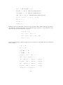
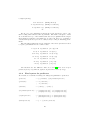
The effect of entering ”COLOR”, ”red”, ”green”, and ”orange” in this wizard is to add the new carrier
set COLOR (section 2.1) and the three constants (section 2.3) red, green, and orange. Finally, it adds
the following axioms (section 2.4):
COLOR = {red, green, orange}
red 6= green
red 6= orange
green 6= orange
If you enter several time the same enumerated set element, you get an error message.
2.3
2.3.1
Constants
Constants Creation Wizard.
In order to activate the constants creation wizard, you have to press the corresponding button in the toolbar
as indicated below:
After pressing that button, the following wizard pops up:
10
You can then enter the names of the constants, and an axiom which can be used to define its type. Here is
an example:
By pressing the ”More Axm.” button you can enter additional axioms. For adding more constants, press
”Add” button. When you’re finished, press button ”OK”.
2.3.2
Direct Editing of Constants.
It is also possible to create (button ”Add”) or remove (button ”Delete”) constants by using the central
editing window. For this, you have first to select the ”Constants” tab of the editor. You can also change
the relative place of a constant: first select it and then press button ”Up” or ”Down”.
As can be seen, two more constants, bit1 and bit2 have been added. Note that this time the axioms
concerning these constants have to be added directly (see next section 2.4).
11
2.4
2.4.1
Axioms
Axioms Creation Wizard.
In order to activate the axioms creation wizard, you have to press the corresponding button in the toolbar
as indicated below:
After pressing that button, the following wizard appears:
You can then enter the axioms you want. If more axioms are needed then press ”More”. When you are
finished, press ”OK”.
2.4.2
Direct Editing of Axioms.
It is also possible to create (button ”Add”) or remove (button ”Delete”) axioms by using the central editing
window. For this, you have first to select the ”Axioms” tab of the editor. You can also change the relative
place of an axiom: first select it and then press button ”Up” or ”Down”.
12
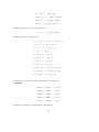
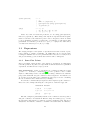
Note that the ”Up” and ”Down” buttons for changing the order of axioms are important for welldefinedness. For example the following axioms in that order
axm1 : y/x = 3
axm2 : x 6= 0
does not allow to prove the well-definedness of y/x = 3. The order must be changed to the following:
axm2 : x 6= 0
axm1 : y/x = 3
The same remark applies to theorems (section 2.5 and 3.4), invariants (section 3.3) and event guards
(section3.5.2)
2.5
2.5.1
Theorems
Theorems Creation Wizard.
In order to activate the theorems creation wizard, you have to press the corresponding button in the toolbar
as indicated below:
13
After pressing that button, the following wizard pops up:
You can then enter the theorems you want. If more theorems are needed then press ”More”. When you
are finished, press ”OK”.
2.5.2
Direct Editing of Theorems.
It is also possible to create (button ”Add”) or remove (button ”Delete”) theorems by using the central
editing window. For this, you have first to select the ”Theorems” tab of the editor. You can also change
the relative place of a theorem: first select it and then press button ”Up” or ”Down”.
14
2.6
Adding Comments
It is possible to add comments to carrier sets, constants, axioms and theorems. For doing so, select the
corresponding modeling element and enter the ”Properties” window as indicated below where it is shown
how to add comments on a certain axiom:
Multiline comments can be added in the editing area labeled ”Comments”.
2.7
Dependencies
By selecting the ”Dependencies” tab of the editor, you obtain the following window:
This allows you to express that the current context is extending other contexts of the current project. In
order to add the name of the context you want to extend, use the combobox which appears at the bottom
of the window and then select the corresponding context name.
15
There is another way to directly create a new context extending an existing context C. Select the context
C in the project window, then press the right mouse key, you will get the following menu:
After pressing the ”Extend” button, the following wizard pops up:
You can then enter the name of the new context which will be made automatically an extension of C.
2.8
Pretty Print
By selecting the ”Pretty Print” tab, you may have a global view of your context as if it would have been
entered through an input text file.
16
3
Anatomy of a Machine
Once a machine is created, a window such as the following appears in the editing area:
You are in the ”Edit” page allowing you to edit elements of the machine, namely dependencies (keywords ”REFINES” and ”SEES”), variables (keyword ”VARIABLES”), invariants (keyword ”INVARIANTS), theorems (keyword ”THEOREMS”), variants (keyword ”VARIANTS”), or events (Keywords
”EVENTS”). These modelling elements can be edited in a way that is similar to what has been explained
for contexts in section 2, it is not repeated here.
It is also possible to do so in a different way as explained in sections 3.1 to 3.6. The creation of these
elements, except dependencies can be made by two distinct methods, either by using wizards or by editing
them directly. In each section, we shall review both methods.
NOTE: The hurried reader can skip these sections and go directly to section 3.7
3.1
Dependencies
The ”Dependencies” window is shown automatically after creating a machine (you can also get it by
selecting the ”Dependencies” tab). This was shown in the previous section so that we do not copy the
screen shot again. As can be seen in this window, two kinds of dependencies can be established: machine
dependency in the upper part and context dependencies in the lower part.
In this section, we only speak of context dependencies (machine dependency will be covered in section 3.8). It corresponds to the ”sees” relationship alluded in section 1. In the lower editing area, you can
select some contexts ”seen” by the current machine.
17
3.2
3.2.1
Variables
Variables Creation Wizard.
In order to activate the variables creation wizard, you have to press the corresponding button in the toolbar
as indicated below:
After pressing that button, the following wizard pops up:
You can then enter the names of the variables, its initialization, and an invariant which can be used to
define its type. By pressing button ”More Inv.” you can enter additional invariants. For adding more
variables, press the ”Add” button. When you’re finished, press the ”OK” button.
3.2.2
Direct Editing of Variables.
It is also possible to create (button ”Add”) or remove (button ”Delete”) variables by using the central
editing window. For this, you have first to select the ”Variables” tab of the editor. You can also change the
relative place of a variable: first select it and then press button ”Up” or ”Down”.
18
3.3
3.3.1
Invariants
Invariants Creation Wizard.
In order to activate the invariants creation wizard, you have to press the corresponding button:
After pressing that button, the following wizard pops up:
You can then enter the invariants you want. If more invariants are needed then press ”More”.
19
3.3.2
Direct Editing of Invariants.
It is also possible to create (button ”Add”) or remove (button ”Delete”) invariants by using the central
editing window. For this, you have first to select the ”Invariants” tab of the editor. You can also change
the relative place of an invariant: first select it and then press button ”Up” or ”Down”.
3.4
3.4.1
Theorems
Theorems Creation Wizard.
In order to activate the theorems creation wizard, you have to press the corresponding button:
After pressing that button, the following wizard pops up:
20
You can then enter the theorems you want. If more theorems are needed then press ”More”. When you
are finished, press the ”OK” button.
3.4.2
Direct Editing of Theorems.
It is also possible to create (button ”Add”) or remove (button ”Delete”) theorems by using the central
editing window. For this, you have first to select the ”Theorems” tab of the editor. You can also change
the relative place of a theorem: first select it and then press button ”Up” or ”Down”.
3.5
3.5.1
Events
Events Creation Wizard.
In order to activate the events creation wizard, you have to press the corresponding button in the toolbar
as indicated below:
21
After pressing that button, the following wizard pops up:
You can then enter the events you want. As indicated, the following elements can be entered: name,
parameters, guards, and actions. More parameters, guards and actions can be entered by pressing the
corresponding buttons. If more events are needed then press ”Add”. Press ”OK” when you’re finished.
Note that an event with no guard is considered to have a true guard. Moreover, an event with no action
is considered to have the ”skip” action.
3.5.2
Direct Editing of Events.
It is also possible to perform a direct creation (button ”Add Event”) of variables by using the central
editing window. For this, you have first to select the ”Events” tab of the editor. You can also change the
relative place of a variable: first select it and then press button ”Up” or ”Down”.
22
Once an event is selected you can add parameters, guards, and actions. The components of an events can
be seen by pressing the little triangle situated on the left of the event name:
As can be seen, event rmv 1 is made of two parameters, x and y, three guards, x ∈ Q, y ∈ Q, and
x 7→ y ∈ k, and one action Q := Q \ {x}. These elements can be modified (select and edit) or removed
(select, right click on the mouse, and press ”Delete”). Similar elements can be added by pressing the
relevant buttons on the right of the window.
23
3.6
Adding Comments
It is possible to add comments to variables, invariants, theorems, events, guards, and actions. For doing so,
select the corresponding modeling element and enter the ”Properties” window as indicated below where
it is shown how one can add comments on a certain guard:
Multiline comments can be added in the editing area labeled ”Comments”.
3.7
Pretty Print
The pretty print of a machine looks like an input file. It is produced as an output of the editing process:
24
3.8
Dependencies: Refining a Machine
A machine can be refined by other ones. This can be done directly by selecting the machine to be refined
in the ”Project Explorer” window. A right click on the mouse yields the following contextual menu:
You then press button ”Refine”. A wizard will ask you to enter the name of the refined machine. The
abstract machine is entirely copied in the refined machine: this is very convenient as, quite often, the
refined machine has lots of elements in common with its abstraction.
3.9
3.9.1
Adding more Dependencies
Abstract Event
The absraction of an event is denoted by a ”Refine Event” element. Most of the time the concrete and
abstract events bear the same name. But, it is always possible to change the name of a concrete event or
the name of its abstraction. If you want to specify the abstraction of an event, first select the ”Event” tab
of the editor and right click on the event name. The following contextual menu will pop up:
25
You have then to choose the ”New Refine Event” option. The abstract event can then be entered by adding
the name of the abstract event: here rmv 1.
3.9.2
Splitting an Event
An abstract event can be split into two or more concrete events by just saying that these events refine the
former (as explained in previous section).
3.9.3
Merging Events
Two or more abstract events can be merged into a single concrete event by saying that the latter refines
all the former. This is done by using several times the approach explained in the previous case. The
constraints is that the abstract events to be merged must have exactly the same actions (including the
labels of these actions). A proof obligation is generated which states that the guard of the concrete event
implies the disjunction of the guards of the abstract events
3.9.4
Witnesses
When an abstract event contains some parameters, the refinement proof obligation involves proving an
existentially quantified statement. In order to simplify the proof, the user is required to give witnesses
for those abstract parameters which are not present in the refinement (those appearing in the refinement
are implicitly taken as witnesses for their corresponding abstract counterparts). Here is an example of an
abstract event (left) and its refinement (right):
26
The parameter x, being common to both the abstraction and the refinement, does not require a witness,
whereas one is needed for abstract parameter y. In order to define the witness, one has first to select the
”Events” tab of the editor for the concrete machine where the concrete event (here rmv 1) is selected.
After a right click, a menu appears in the window as indicated:
You press button ”New Witness” and then you enter the parameter name (here y) and a predicate involving
y (here y = b) as indicated below
Most of the time, the predicate is an equality as in the previous example, meaning that the parameter is
defined in a deterministic way. But it can also be any predicate, in which case the parameter is defined in
a non-deterministic way.
3.9.5
Variant
New events can be defined in a concrete machine. Such events have no abstract counterparts. They must
refine the implicit ”empty” abstract event which does nothing.
Some of the new events can be selected to decrease a variant so that they do not take control for ever.
Such events are said to be CONVERGENT. In order to make a new event CONVERGENT, select it in the
”Events” tab and open the ”Properties” window. You can edit the ”conv.” area. There are three options:
ORDINARY (the default), CONVERGENT, or ANTICIPATED. The latter corresponds to a new event
which is not yet declared to be CONVERGENT but will be in a subsequent refinement.
27
In order to define the variant, use the variant wizard as shown below:
After pressing that button, the following wizard will pop up
You can enter the variant and then press ”OK”. The variant is either a natural number expression or a
finite set expression.
4
Saving a Context or a Machine
Once a machine or context is (possibly partly only) edited, you can save it by using the following button:
4.1
Automatic Tool Invocations
Once a ”Save” is done, three tools are called automatically, these are:
• the Static Checker,
• the Proof Obligation Generator,
• the Auto-Prover.
This can take a certain time. A ”Progress” window can be opened at the bottom right of the screen to see
which tools are working (most of the time, it is the auto-prover).
28
4.2
Errors. The Problems Window
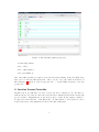
When the Static Checker discovers an error in a project, a little ”x” is added to this project and to the
faulty component in the ”Project Explorer” window as shown in the following screen shot:
The error itself is shown by opening the ”Problems” window.
By double-clicking on the error statement, you are transferred automatically into the place where the error
has been detected so that you can correct it easily as shown below:
29
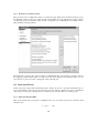
4.3
Preferences for the Auto-prover
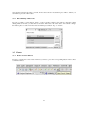
The auto-prover can be configured by means of a preference page, which can be obtained as follows:
press the ”Window” button on the top tooolbar. On the coming menu, press the ”Preferences” button. On
the coming menu, press the ”Event-B” menue, then the ”Sequent Prover’, and finally the ”Auto-Tactic”
button. This yields the following window:
On the left part you can see the ordered sequence of individual tactics composing the auto-prover, whereas
the right part contains further tactics you can incorporate in the left part. By selecting a tactic you can
move it from on part to the other or change the order in the left part.
30
5
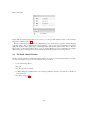
The Proof Obligation Explorer
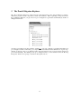
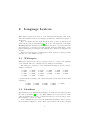
The ”Proof Obligation Explorer” window has the same main entries as the ”Project Explorer” window,
namely the projects and its components (context and machines). When expanding a component in the
Proof Obligation Explorer you get a list of its proof obligations as generated automatically by the Proof
Obligation Generator:
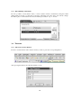
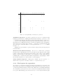
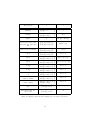
As can be seen in this screen shot, machine ”celebrity 1” of project ”celebrity” is expanded. We find seven
proof obligations. Each of them has got a compound name as indicated in the tables below. A green logo
situated on the left of the proof obligation name states that it has been proved (an A means it has been
proved automatically). By clicking on the proof obligation name, you are transferred into the Proving
Perspective which we are going to describe in subsequent sections.
31
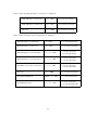
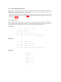
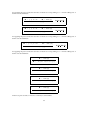
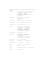
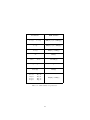
Next is a table describing the names of context proof obligations:
Well-definedness of an Axiom
axm / WD
axm is the axiom name
Well-definedness of a Theorem
thm / WD
thm is the theorem name
Theorem
thm / THM
thm is the theorem name
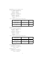
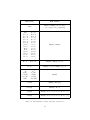
Next is a table showing the name of machine proof obligations:
Well-definedness of an Invariant
inv / WD
inv is the invariant name
Well-definedness of a Theorem
thm / WD
thm is the theorem name
Well-definedness of an event Guard
evt / grd / WD
evt is the event name
grd is the guard name
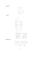
Well-definedness of an event Action
evt / act / WD
evt is the event name
act is the action name
Feasibility of a non-det. event Action
evt / act / FIS
evt is the event name
act is the action name
Theorem
thm / THM
thm is the theorem name
Invariant Establishment
INIT. / inv / INV
inv is the invariant name
Invariant Preservation
evt / inv / INV
32
evt is the event name
inv is the invariant name
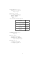
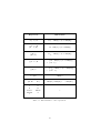
Next are the proof obligations concerned with machine refinements:
evt is the concrete event name
grd is the abstract guard name
Guard Strengthening
evt / grd / GRD
Guard Strengthening (merge)
evt / MRG
Action Simulation
evt / act / SIM
evt is the concrete event name
act is the abstract action name
Equality of a preserved Variable
evt / v / EQL
evt is the concrete event name
v is the preserved variable
evt is the concrete event name
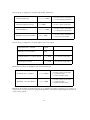
Next are the proof obligations concerned with the new events variant:
Well definedness of Variant
VWD
Finiteness for a set Variant
FIN
Natural number for a numeric Variant
evt / NAT
evt is the new event name
Decreasing of Variant
evt / VAR
evt is the new event name
Finally, here are the proof obligations concerned with witnesses:
Well definedness of Witness
evt / p / WWD
evt is the concrete event name
p is parameter name
or a primed variable name
Feasibility of non-det. Witness
evt / p / WFIS
evt is the concrete event name
p is parameter name
or a primed variable name
Remark: At the moment, the deadlock freeness proof obligation generation is missing. If you need it, you
can generate it yourself as a theorem saying the the disjunction of the abstract guards imply the disjunction
of the concrete guards.
33
6
The Proving Perspective
The Proving Perspective is made of a number of windows: the proof tree, the goal, the selected hypotheses,
the proof control, the proof information, and the searched hypotheses. In subsequent sections, we study
these windows, but before that let us see how one can load a proof.
6.1
Loading a Proof
In order to load a proof, enter the Proof Obligation window, select the project, select and expand the
component, finally select the proof obligation: the corresponding proof will be loaded. As a consequence:
• the proof tree is loaded in the Proof Tree window. As we shall see in section 6.2, each node of the
proof tree is associated with a sequent.
• In case the proof tree has some ”pending” nodes (whose sequents are not discharged yet) then the
sequent corresponding to the first pending node is decomposed: its goal is loaded in the Goal window (section 6.3), whereas parts of its hypotheses (the ”selected” ones) are loaded in the Selected
Hypotheses window (section 6.3).
• In case the proof tree has no pending node, then the sequent of the root node is loaded as explained
previously.
6.2
6.2.1
The Proof Tree
Description of the Proof Tree
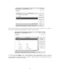
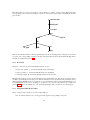
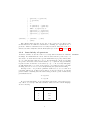
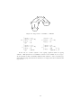
The proof tree can be seen in the corresponding window as shown in the following screen shot:
34
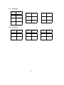
Each line in the proof tree corresponds to a node which is a sequent. A line is right shifted when the
corresponding node is a direct descendant of the node of the previous line. Here is an illustration of the
previous tree:
auto rewrite
forall goal
==> goal
ovr
eh
PP
ah
T goal
eh
ML
hyp
Each node is labelled with a comment explaining how it can be discharged. By selecting a node in the
proof tree, the corresponding sequent is decomposed and loaded in the Goal and Selected Hypotheses
windows as explained in section 6.1.
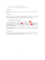
6.2.2
Decoration
The leaves of the tree are decorated with three kinds of logos:
√
• a green logo with a ” ” in it means that this leaf is discharged,
• a red logo with a ”?” in it means that this leaf is not discharged,
• a blue logo with a ”R” in it means that this leaf has been reviewed.
Internal nodes in the proof tree are decorated in the same (but lighter) way. Note that a ”reviewed” leaf is
one that is not discharged yet by the prover. Instead, it has been ”seen” by the user who decided to have it
discharged later. Marking nodes as ”reviewed” is very convenient in order to perform an interactive proof
in a gradual fashion. In order to discharge a ”reviewed” node, select it and prune the tree at that node
(section 6.2.5): the node will become ”red” again (undischarged) and you can now try to discharge it.
6.2.3
Navigation within the Proof Tree
On top of the proof tree window one can see three buttons:
• the ”G” buttons allows you to see the goal of the sequent corresponding to the node
35
• the ”+” button allows you to fully expand the proof tree
• the ”-” allows you to fully collapse the tree: only the root stays visible.
6.2.4
Hiding
The little triangle next to each node in the proof tree allows you to expand or collapse the subtree starting
at that node.
6.2.5
Pruning
The proof tree can be pruned from a node: it means that the subtree starting at that node is eliminated.
The node in question becomes a leaf and is red decorated. This allows you to resume the proof from that
node. After selecting a sequent in the proof tree, pruning can be performed in two ways:
• by right-clicking and then selecting ”Prune”,
• by pressing the ”Scissors” button in the proof control window (section 6.4).
Note that after pruning, the post-tactic (section 6.8) is not applied to the new current sequent: if needed
you have to press the ”post-tactic” button in the Proof Control window (section 6.4). This happens in
particular when you want to redo a proof from the beginning: you prune the proof tree from the root node
and then you have to press the ”post-tactic” button in order to be in exactly the same situation as the one
delivered automatically initially.
When you want to redo a proof from a certain node, it might be advisable to do it after copying the
tree so that in case your new proof fails you can still resume the previous situation by pasting the copied
version (see next section).
6.2.6
Copy/Paste
By selecting a node in the proof tree and then clicking on the right key of the mouse, you can copy the
part of the proof tree starting at that sequent: it can later be pasted in the same way. This allows you to
reuse part of a proof tree in the same (or even another) proof.
36
6.3
Goal and Selected Hypotheses
The ”Goal” and ”Selected Hypotheses” windows display the current sequent you have to prove at a given
moment in the proof. Here is an example:
A selected hypothesis can be deselected by first clicking in the box situated next to it (you can click on
several boxes) and then by pressing the red (-) button at the top of the selected hypothesis window:
37
Here is the result:
Notice that the deselected hypotheses are not lost: you can get them back by means of the Searched
Hypotheses window (section 6.7).
The three other buttons next to the red (-) button allow you to do the reverse operation, namely keeping
some hypotheses. The (ct) button next to the goal allows you to do a proof by contradiction: pressing it
makes the negation of the goal being a selected hypothesis whereas the goal becomes ”false”. The (ct)
button next to a selected hypothesis allows you to do another kind of proof by contradiction: pressing it
makes the negation of the hypothesis the goal whereas the negated goal becomes an hypothesis.
6.4
The Proof Control Window
The Proof Control window contains the buttons which you can use to perform an interactive proof. Next
is a screen shot where you can see successively from top to bottom:
• some selected hypotheses,
• the goal,
• the ”Proof Control” window,
• a small editing area within which you can enter parameters used by some buttons of the Proof
Control window
• the smiley (section 6.5)
38
The Proof Control window offers a number of buttons which we succinctly describe from left to right:
• (nPP): the prover newPP attempts to prove the goal (other cases in the list),
• (p0): the prover PP attempts to prove the goal (other cases in the list)
• (R) review: the user forces the current sequent to be discharged, it is marked as being reviewed (it’s
logo is blue-colored)
• (dc) proof by cases: the goal is proved first under the predicate written in the editing area and then
under its negation,
• (ah) lemma: the predicate in the editing area is proved and then added as a new selected hypothesis,
• (ae) abstract expression: the expression in the editing area is given a fresh name,
• the auto-prover attempts to discharge the goal. The auto-prover is the one which is applied automatically on all proof obligations (as generated automatically by the proof obligation generator after a
”save”) without any intervention of the user. With this button, you can call yourself the auto-prover
within an interactive proof.
• the post-tactic is executed (see section 6.8),
• lasso: load in the Selected Hypotheses window those unseen hypotheses containing identifiers
which are common with identifiers in the goal and selected hypotheses,
• backtrack form the current node (i.e., prune its parent),
• scissors: prune the proof tree from the node selected in the proof tree,
• show (in the Search Hypotheses window) hypotheses containing the character string as in the editing
area,
• show the Cache Hypotheses window,
• load the previous non-discharged proof obligation,
39
• load the next non-discharged proof obligation,
• (i) show information corresponding to the current proof obligation in the corresponding window.
This information correspond to the elements that took directly part in the proof obligation generation
(events, invariant, etc.),
• goto the next pending node of the current proof tree,
• load the next reviewed node of the current proof tree.
6.5
The Smiley
The smiley can take three different colors: (1) red, meaning that the proof tree contains one or more
non-discharged sequents, (2) blue, meaning that all non-discharged sequents of the proof tree have been
reviewed, (3) green, meaning that all sequents of the proof tree are discharged.
6.6
The Operator ”Buttons”
In the goal and in the selected, searched, or cache hypotheses some operators are colored in red. It means
that they are ”buttons” you can press. When doing so, the meaning (sometimes several) is shown in a
menu where you can select various options. The operation performed by these options is described in
sections 6.9.1 and 6.9.2.
6.7
The Search Hypotheses Window
A window is provided which contains the hypotheses having a character string in common with the one
in the editing area. For example, if we search for hypotheses involving the character string ”cr”, then after
pressing the ”search hypothesis” button in the proof control window, we obtain the following:
Such hypotheses can be moved to the ”Selected Hypotheses” window (button (+)) or removed from the
”Search Hypotheses” window (button (-)). As for the selected hypotheses, other buttons situated next to
the previous ones, allow you to move or remove all hypotheses. By pressing the (ct) button the negation
of the corresponding hypothesis becomes the new goal.
40
6.8
The Automatic Post-tactic
In this section, we present the various rewrite or inference rules which are applied automatically as a
systematic post-tactic after each proof step. Note that the post-tactic can be disabled by using the ”P
/”
button situated on the right of the proof control window.
The post-tactic is made of two different rules: rewrite rules, which are applied on any sub-formula
of the goal or selected hypotheses (section 6.8.1) and inference rules which are applied on the current
sequent (section 6.8.2).
6.8.1
Rewrite rules
The following rewrite rules are applied automatically in a systematic fashion from left to right either in
the goal or in the selected hypotheses. They all correspond to predicate logical equivalences or expression
equalities and result in simplifications. They are sorted according to their main purpose.
Conjunction
P ∧ . . . ∧ > ∧ . . . ∧ Q == P ∧ . . . ∧ Q
P ∧ . . . ∧ ⊥ ∧ . . . ∧ Q == ⊥
P ∧ . . . ∧ Q ∧ . . . ∧ ¬ Q ∧ . . . ∧ R == ⊥
P ∧ . . . ∧ Q ∧ . . . ∧ Q ∧ . . . ∧ R == P ∧ . . . ∧ Q ∧ . . . ∧ R
Disjunction
P ∨ . . . ∨ > ∨ . . . ∨ Q == >
P ∨ . . . ∨ ⊥ ∨ . . . ∨ Q == P ∨ . . . ∨ Q
P ∨ . . . ∨ Q ∨ . . . ∨ ¬ Q ∨ . . . ∨ R == >
P ∨ . . . ∨ Q ∨ . . . ∨ Q ∨ . . . ∨ R == P ∨ . . . ∨ Q ∨ . . . ∨ R
Implication
> ⇒ P == P
⊥ ⇒ P == >
P ⇒ > == >
P ⇒ ⊥ == ¬ P
P ⇒ P == >
41
Equivalence
P ⇔ > == P
> ⇔ P == P
P ⇔ ⊥ == ¬ P
⊥ ⇔ P == ¬ P
P ⇔ P == >
Negation
¬ > == ⊥
¬ ⊥ == >
¬ ¬ P == P
E 6= F == ¬ E = F
E∈
/ F == ¬ E ∈ F
E 6⊂ F == ¬ E ⊂ F
E 6⊆ F == ¬ E ⊆ F
¬ a ≤ b == a > b
¬ a ≥ b == a < b
¬ a > b == a ≤ b
¬ a < b == a ≥ b
¬ (E = FALSE) ==
(E = TRUE)
¬ (E = TRUE) ==
(E = FALSE)
¬ (FALSE = E) ==
(TRUE = E)
¬ (TRUE = E) ==
(FALSE = E)
Quantification
∀x · ( P ∧ Q) == (∀x · P ) ∧ (∀x · Q)
∃x · ( P ∨ Q) == (∃x · P ) ∨ (∃x · Q)
∀ . . . , z, . . . · P (z) == ∀z · P (z)
∃ . . . , z, . . . · P (z) == ∃z · P (z)
42
Equality
E = E == >
E 6= E == ⊥
E 7→ F = G 7→ H == E = G ∧ F = H
TRUE = FALSE ==
⊥
FALSE = TRUE ==
⊥
Set Theory
S ∩ . . . ∩ ∅ ∩ . . . ∩ T == ∅
S ∩ . . . ∩ T ∩ . . . ∩ T ∩ . . . ∩ U == S ∩ . . . ∩ T ∩ . . . ∩ U
S ∪ . . . ∪ ∅ ∪ . . . ∪ T == S ∪ . . . ∪ T
S ∪ . . . ∪ T ∪ . . . ∪ T ∪ . . . ∪ U == S ∪ . . . ∪ T ∪ . . . ∪ U
∅ ⊆ S == >
S ⊆ S == >
E ∈ ∅ == ⊥
B ∈ {A, . . . , B, . . . , C} == >
{A, . . . , B, . . . , B, . . . , C} == {A, . . . , B, . . . , C}
E ∈ { x | P (x) } == P (E)
S \ S == ∅
S \ ∅ == S
∅ \ S == ∅
r[∅] == ∅
dom(∅) == ∅
ran(∅) == ∅
r−1−1 == r
dom({x 7→ a, . . . , y 7→ b} == {x, . . . , y}
ran({x 7→ a, . . . , y 7→ b} == {a, . . . , b}
43
(f − ... − {E 7→ F })(E) == F
E ∈ {F } == E = F
where F is a single expression
(S × {F })(x) == F
where F is a single expression
{E} = {F } == E = F
where E and F are single expressions
{x 7→ a, . . . , y 7→ b}−1 == {a 7→ x, . . . , b 7→ y}
Ty = ∅ == ⊥
∅ = Ty == ⊥
t ∈ Ty == >
In the three previous rewrite rules, Ty denotes a type expression, that is either a basic type (Z, BOOL,
any carrier set), or P(type expression), or type expression×type expression, or type expression↔type
expression, and t denotes an expression of type Ty.
U \ U \ S == S
S ∪ . . . ∪ U ∪ . . . ∪ T == U
S ∩ . . . ∩ U ∩ . . . ∩ T == S ∩ . . . ∩ T
S \ U == ∅
In the four previous rules, S and T are supposed to be of type P(U ) (U thus takes the rôle of a universal
set for S and T ).
r ; ∅ == ∅
∅ ; r == ∅
f (f −1 (E)) == E
f −1 (f (E)) == E
S ⊆ A ∪ . . . ∪ S ∪ . . . ∪ B == >
A ∩ . . . ∩ S ∩ . . . ∩ B ⊆ S == >
A ∪ . . . ∪ B ⊆ S == A ⊆ S ∧ . . . ∧ B ⊆ S
S ⊆ A ∩ . . . ∩ B == S ⊆ A ∧ . . . ∧ S ⊆ B
A ∪ . . . ∪ B ⊂ S == A ⊂ S ∧ . . . ∧ B ⊂ S
S ⊂ A ∩ . . . ∩ B == S ⊂ A ∧ . . . ∧ S ⊂ B
A \ B ⊆ S == A ⊆ B ∪ S
44
Finiteness
finite (∅) == >
finite ({a, . . . , b}) == >
finite (S ∪ T ) == finite (S) ∧ finite (T )
finite (P(S)) == finite (S)
finite (S × T ) == S = ∅ ∨ T = ∅ ∨ (finite (S) ∧ finite (T ))
finite (r−1 ) == finite (r)
finite (a .. b) == >
Cardinality
card(∅) == 0
card ({E}) == 1
card (P(S)) == 2card(S)
card (S × T ) == card(S) ∗ card(T )
card (S \ T ) == card(S) − card (S ∩ T )
card (S ∪ T ) == card(S) + card(T ) − card (S ∩ T )
card (S) = 0 == S = ∅
0 = card (S) == S = ∅
¬ card (S) = 0 == ¬ S = ∅
¬ 0 = card (S) == ¬ S = ∅
card (S) > 0 == ¬ S = ∅
0 < card (S) == ¬ S = ∅
card (S) = 1 == ∃x · S = {x}
1 = card (S) == ∃x · S = {x}
45
Arithmetic
E + . . . + 0 + . . . + F == E + . . . + F
E − 0 == E
0 − E == −E
−(−E) == E
E − E == 0
E ∗ . . . ∗ 1 ∗ . . . ∗ F == E ∗ . . . ∗ F
E ∗ . . . ∗ 0 ∗ . . . ∗ F == 0
(−E) ∗ . . . ∗ (−F ) == E ∗ . . . ∗ F
(if an even number of -)
(−E) ∗ . . . ∗ (−F ) == − (E ∗ . . . ∗ F )
(if an odd number of -)E/1 == E
0/E == 0
(−E)/(−F ) == E/F
E 1 == E
E 0 == 1
1E == 1
−(i) == (−i) where i is a literal
−((−i)) == i where i is a literal
i = j == > or ⊥ (computation)
where i and j are literals
i ≤ j == > or ⊥ (computation)
where i and j are literals
i < j == > or ⊥ (computation)
where i and j are literals
i ≥ j == > or ⊥ (computation)
where i and j are literals
i > j == > or ⊥ (computation)
where i and j are literals
E ≤ E == >
E < E == ⊥
E ≥ E == >
E > E == ⊥
46
6.8.2
Automatic inference rules
The following inference rules are applied automatically in a systematic fashion at the end of each proof
step. They have the following possible effects:
• they discharge the goal,
• they simplify the goal and add a selected hypothesis,
• they simplify the goal by decomposing it into several simpler goals,
• they simplify a selected hypothesis,
• they simplify a selected hypothesis by decomposing it into several simpler selected hypotheses.
47
Axioms
HYP
H, P ` P
H, Q ` P ∨ . . . ∨ Q ∨ . . . ∨ R
H, P, ¬ P ` Q
CNTR
FALSE HYP
H, ⊥ ` P
HYP OR
TRUE GOAL
H ` >
Simplification
H, P ` Q
H, P, P ` Q
DBL HYP
Conjunction
H, P, Q ` R
H, P ∧ Q ` R
H ` P
AND L
H ` Q
H ` P ∧ Q
AND R
Implication
H, Q, P ∧ . . . ∧ R ⇒ S ` T
H, Q, P ∧ . . . ∧ Q ∧ . . . ∧ R ⇒ S ` T
IMP L1
H, P ` Q
H ` P⇒Q
H, P ⇒ Q, P ⇒ R ` S
H, P ⇒ Q ∧ R ` S
IMP R
H, P ⇒ R, Q ⇒ R ` S
IMP AND L
H, P ∨ Q ⇒ R ` S
48
IMP OR L
Negation
H, E ∈ {a, . . . , c} `
P
H, E ∈ {a, . . . , b, . . . , c}, ¬ (E = b) ` P
H, E ∈ {a, . . . , c} `
P
H, E ∈ {a, . . . , b, . . . , c}, ¬ (b = E) ` P
Quantification
H, P(x) ` Q
XST L
(x not free in H and Q)
H, ∃ x · P(x) ` Q
H ` P(x)
ALL R
(x not free in H)
H ` ∀x · P(x)
Equality
H(E) `
H(E) `
P(E)
H(x), x = E ` P(x)
EQL LR
P(E)
H(x), E = x ` P(x)
In the last two rules x is a variable which is not free in E
49
EQL RL
6.8.3
Preferences for the Post-tactic
The post-tactic can be configured by means of a preference page which can be obtained as follows: press
the ”Window” button on the top tooolbar. On the coming menu, press the ”Preferences” button. On the
coming menu, press the ”Event-B” menue, then the ”Sequent Prover’, and finally the ”Post-Tactic” button.
This yields the following window:
In the left part you can see the ordered sequence of individual tactics composing the post-tactic, whereas
the right part contains further tactics you can incorporate in the left part. By selecting a tactic you can
move it from on part to the other or change the order in the left part.
6.9
Interactive Tactics
In this section, the rewrite rules and inference rules, which you can use to perform an interactive proof,
are presented. Each of these rules can be invoked by pressing ”buttons” which corresponds to emphasized
(red) operators in the goal or the hypotheses. A menu is proposed when there are several options.
6.9.1
Interactive Rewrite Rules
Most of the rewrite rules correspond to distributive laws. For associative operators in connection with
such laws as in:
P ∧ (Q ∨ . . . ∨ R)
50
it has been decided to put the ”button” on the first associative/commutative operator (here ∨). Pressing that
button will generate a menu: the first option of this menu will be to distribute all associative/commutative
operators, the second option will be to distribute only the first associative/commutative operator. In the
following presentation, to simplify matters, we write associative/commutative operators with two parameters only, but it must always be understood implicitly that we have a sequence of them. For instance, we
shall never write Q ∨ . . . ∨ R but Q ∨ R instead. Rules are sorted according to their purpose.
51
Conjunction
P ∧ (Q ∨ R) == (P ∧ Q) ∨ (P ∧ R)
Disjunction
P ∨ (Q ∧ R) == (P ∨ Q) ∧ (P ∨ R)
P ∨ Q ∨ . . . ∨ R == ¬ P ⇒ (Q ∨ . . . ∨ R)
Implication
P ⇒ Q == ¬ Q ⇒ ¬P
P ⇒ (Q ⇒ R) == P ∧ Q ⇒ R
P ⇒ (Q ∧ R) == (P ⇒ Q) ∧ (P ⇒ R)
P ∨ Q ⇒ R == (P ⇒ R) ∧ (Q ⇒ R)
Equivalence
P ⇔ Q == (P ⇒ Q) ∧ (Q ⇒ P )
Negation
¬ (P ∧ Q) == ¬ P ∨ ¬ Q
¬ (P ∨ Q) == ¬ P ∧ ¬ Q
¬ (P ⇒ Q) == P ∧ ¬ Q
¬ ∀x · P == ∃x · ¬ P
¬ ∃x · P == ∀x · ¬ P
¬ (S = ∅) == ∃x · x ∈ S
Set Theory
Most of the rules are concerned with simplifying set membership predicates.
E 7→ F ∈ S × T == E ∈ S ∧ F ∈ T
E ∈ P(S) == E ⊆ S
S ⊆ T == ∀x · ( x ∈ S ⇒ x ∈ T )
In the previous rule, x denotes several variables when the type of S and T is a Cartesian product.
52
E ∈ S ∪ T == E ∈ S ∨ E ∈ T
E ∈ S ∩ T == E ∈ S ∧ E ∈ T
E ∈ S \ T == E ∈ S ∧ ¬ (E ∈ T )
E ∈ {A, . . . , B}
==
E = A ∨ ... ∨ E = B
E ∈ union (S) == ∃s · s ∈ S ∧ E ∈ s
S
E ∈ ( x · x ∈ S ∧ P | T ) == ∃x · x ∈ S ∧ P ∧ E ∈ T
E ∈ inter (S) == ∀s · s ∈ S ⇒ E ∈ s
T
E ∈ ( x · x ∈ S ∧ P | T ) == ∀x · x ∈ S ∧ P ⇒ E ∈ T
E ∈ dom(r) == ∃y · E 7→ y ∈ r
F ∈ ran(r) == ∃x · x 7→ F ∈ r
E 7→ F ∈ r−1 == F 7→ E ∈ r
E 7→ F ∈ S r == E ∈ S ∧ E 7→ F ∈ r
E 7→ F ∈ r T == E 7→ F ∈ r ∧ F ∈ T
E 7→ F ∈ S − r == E ∈
/ S ∧ E 7→ F ∈ r
E 7→ F ∈ r − T == E 7→ F ∈ r ∧ F ∈
/T
F ∈ r[w] == ∃x · x ∈ w ∧ x 7→ F ∈ r
E 7→ F ∈ (p ; q) == ∃x · E 7→ x ∈ p ∧ x 7→ F ∈ q
p
− q == (dom (q) − p) ∪ q
E 7→ F ∈ id (S) == E ∈ S ∧ F = E
E 7→ (F 7→ G) ∈ p ⊗ q == E 7→ F ∈ p ∧ E 7→ G ∈ q
(E 7→ G) 7→ (F 7→ H) ∈ p k q == E 7→ F ∈ p ∧ G 7→ H ∈ q
r∈S←
↔ T == r ∈ S ↔ T ∧ dom(r) = S
r∈S↔
→ T == r ∈ S ↔ T ∧ ran(r) = T
r∈S↔
↔ T == r ∈ S ↔ T ∧ dom(r) = S ∧ ran(r) = T
f ∈S→
7 T == f ∈ S ↔ T ∧ ∀x, y, z·x 7→ y ∈ f ∧ x 7→ z ∈ f ⇒ y = z
f ∈ S → T == f ∈ S →
7 T ∧ dom(f ) = S
f ∈S
7 T == f ∈ S →
7 T ∧ f −1 ∈ T →
7 S
53
f ∈ S T == f ∈ S 7 T ∧ dom(f ) = S
f ∈S
7 T == f ∈ S →
7 T ∧ ran(f ) = T
f ∈ S T == f ∈ S 7 T ∧ dom(f ) = S
f ∈S
T == f ∈ S T ∧ ran(f ) = T
(p ∪ q)−1 == p−1 ∪ q −1
(p ∩ q)−1 == p−1 ∩ q −1
(s r)−1 == r−1 s
(s − r)−1 == r−1 −s
(r s)−1 == s r−1
(r − s)−1 == s r−1
(p ; q)−1 == q −1 ; p−1
(s ∪ t) r == (s r) ∪ (t r)
(s ∩ t) r == (s r) ∩ (t r)
(s ∪ t) − r == (s − r) ∩ (t − r)
(s ∩ t) − r == (s − r) ∪ (t − r)
s (p ∪ q) == (s p) ∪ (s q)
s (p ∩ q) == (s p) ∩ (s q)
s
− (p ∪ q) == (s − p) ∪ (s − q)
s
− (p ∩ q) == (s − p) ∩ (s − q)
r (s ∪ t) == (r s) ∪ (r t)
r (s ∩ t) == (r s) ∩ (r t)
r
− (s ∪ t) == (r − s) ∩ (r − t)
r
− (s ∩ t) == (r − s) ∪ (r − t)
(p ∪ q) s == (p s) ∪ (q s)
(p ∩ q) s == (p s) ∩ (q s)
(p ∪ q) − s == (p − s) ∪ (q − s)
(p ∩ q) − s == (p − s) ∩ (q − s)
r[S ∪ T ] == r[S] ∪ r[T ]
54
(p ∪ q)[S] == p[S] ∪ q[S]
dom(p ∪ q) == dom(p) ∪ dom(q)
ran(p ∪ q) == ran(p) ∪ ran(q)
S ⊆ T == (U \ T ) ⊆ (U \ S)
In the previous rule, the type of S and T is P(U ).
S = T == S ⊆ T ∧ T ⊆ S
In the previous rule, S and T are sets
S ⊆ A \ B == S ⊆ A ∧ S ∩ B = ∅
p ; (q ∪ r) == (p ; q) ∪ (p ; r)
(q ∪ r) ; p == (q ; p) ∪ (r ; p)
(p ; q)[s] == q[p[s]]
(s p) ; q == s (p ; q)
(s − p) ; q == s − (p ; q)
p ; (q s) == (p ; q) s
p ; (q − s) == (p ; q) −s
U \ (S ∩ T ) == (U \ S) ∪ (U \ T )
U \ (S ∪ T ) == (U \ S) ∩ (U \ T )
U \ (S \ T ) == (U \ S) ∪ T
In the three previous rules, S and T are supposed to be of type P(U ).
Cardinality
card (S) ≤ card(T ) == S ⊆ T
card (S) ≥ card(T ) == T ⊆ S
card (S) < card(T ) == S ⊂ T
card (S) > card(T ) == T ⊂ S
card (S) = card(T ) == S = T
In the five previous rules, S and T must be of the same type.
55
6.9.2
Interactive Inference rules
Disjunction
H, P ` R
...
H, Q ` R
CASE
H, P ∨ . . . ∨ Q ` R
Implication
H ` P
H, P, Q ` R
MH
H, P ⇒ Q ` R
H ` ¬Q
H, ¬ Q, ¬ P ` R
HM
H, P ⇒ Q ` R
Equivalence
H(Q), P ⇔ Q ` G(Q)
H(P), P ⇔ Q ` G(P)
EQV
postponed
Set Theory
H, G = E, P(F ) ` Q
H, ¬ (G = E), P(f (G)) ` Q
H, P((f − {E 7→ F })(G)) ` Q
H, G = E ` Q(F )
H, ¬ (G = E) ` Q(f (G))
H ` Q((f − {E 7→ F })(G))
H, G ∈ dom(g), P(g(G)) ` Q
OV L
OV R
H, ¬ G ∈ dom(g), P(f (G)) ` Q
H, P((f − g)(G)) ` Q
56
OV L
H, G ∈ dom(g) ` Q(g(G))
H, ¬ G ∈ dom(g) ` Q(f (G))
OV R
H ` Q((f − g)(G))
In the four previous rules the − operator must appear at the ”top level”
H ` f −1 ∈ A →
7 B
H ` Q(f [S] ∩ f [T ])
H ` Q(f [S ∩ T ])
H ` f ∈A→
7 B
H ` Q(f −1 [S] \ f −1 [T ])
H ` Q(f −1 [S \ T ])
∩DIS R
\DIS R
In the two previous rules, the occurrence of f −1 must appear at the ”top level”. Moreover A and B denote
some type. Similar left distribution rules exist
H ` WD(Q({f (E)}))
H ` Q({f (E)})
H ` Q(f [{E}])
SIM R
In the previous rule, the occurrence of f must appear at the ”top level”. A similar left simplification rule
exists.
H ` WD(Q(g(f (x))))
H ` Q(g(f (x)))
H ` Q((f ; g)(x))
SIM R
In the previous rule, the occurrence of f ; g must appear at the ”top level”. A similar left simplification
rule exists.
Finiteness
H ` S⊆T
H ` finite (T )
H ` finite (S)
fin⊆ R
For applying the previous rule, the user has to write the set corresponding to T in the editing area of the
Proof Control Window.
57
H ` finite (S) ∨ . . . ∨ finite (T )
H ` finite (S ∩ . . . ∩ T )
H ` finite (S)
H ` finite (S \ T )
H ` r ∈ S↔T
H ` finite (S)
fin∩ R
fin\ R
H ` finite (T )
H ` finite (r)
fin rel R
For applying the previous rule, the user has to write the set corresponding to S ↔ T in the editing area of
the Proof Control Window.
H ` finite (r)
H ` finite (r[s])
H ` finite (r)
H ` finite (ran(r))
H ` finite (r)
H ` finite (dom(r))
H ` f ∈ S→
7 T
fin rel img R
fin rel ran R
fin rel dom R
H ` finite (S)
H ` finite (f )
fin fun1 R
For applying the previous rule, the user has to write the set corresponding to S →
7 T in the editing area of
the Proof Control Window.
H ` f −1 ∈ S →
7 T
H ` finite (S)
H ` finite (f )
58
fin fun2 R
For applying the previous rule, the user has to write the set corresponding to S →
7 T in the editing area of
the Proof Control Window.
H ` f ∈ S→
7 T
H ` finite (s)
H ` finite (f [s])
H ` f ∈ S→
7 T
H ` finite (S)
H ` finite (ran(f ))
fin fun img R
fin fun ran R
For applying the previous rule, the user has to write the set corresponding to S →
7 T in the editing area of
the Proof Control Window.
H ` f −1 ∈ S →
7 T
H ` finite (S)
H ` finite (dom(f ))
fin fun dom R
For applying the previous rule, the user has to write the set corresponding to S →
7 T in the editing area of
the Proof Control Window.
H ` finite(S)
H ` ∃n · (∀x · x ∈ S ⇒ n ≤ x)
H ` finite(S)
H ` ∃n · (∀x · x ∈ S ⇒ x ≥ n)
H ` finite(S)
H ` ∃n · (∀x · x ∈ S ⇒ n ≥ x)
H ` finite(S)
H ` ∃n · (∀x · x ∈ S ⇒ x ≤ n)
In the four previous rules, S must not contain any bound variable.
59
H ` ∃n · (∀x · x ∈ S ⇒ n ≤ x)
H ` S ⊆ Z \ N1
H ` finite(S)
H ` ∃n · (∀x · x ∈ S ⇒ x ≤ n)
H ` S⊆N
H ` finite(S)
Cardinality
H, a ≤ b ` Q(b − a + 1)
H, b < a ` Q(0)
H ` Q(card (a .. b))
H, a ≤ b, P(a − b + 1) ` Q
H, b < a, P(0) ` Q
H, P(card (a .. b)) ` Q
In the two previous rules, card(a .. b) must appear at ”top-level”.
H ` P(S ⊆ T )
H ` P(card (S) ≤ card(T ))
There are similar rules for other cases
A
The Mathematical Language
The syntax, type-checking and well-definedness conditions of the mathematical language are described in
a separate document entitled ”The Event-B Mathematical Language”.
B
ASCII Representations of the Mathematical Symbols
The mathematical symbols used in the Event-B mathematical language are Unicode characters, beyond
the ASCII subset. These characters are not always easy to input with a regular keyboard. To help users
enter these characters, a list of standard input strings have been defined. When any of these strings is
entered, it is automatically converted by the user interface to the corresponding Unicode character (i.e.,
mathematical symbol).
60
B.1
B.2
B.3
Atomic Symbols
ASCII
Symbol
ASCII
Symbol
ASCII
Symbol
true
>
NAT
N
TRUE
TRUE
false
⊥
NAT1
N1
FALSE
FALSE
INT
Z
BOOL
BOOL
{}
∅
Unary Operators
ASCII
Symbol
ASCII
Symbol
ASCII
Symbol
not
¬
union
union
prj2
prj2
finite
finite
inter
inter
id
id
card
card
dom
dom
min
min
POW
P
ran
ran
max
max
POW1
P1
prj1
prj1
-
−
ASCII
Symbol
ASCII
Symbol
Assignment Operators
ASCII
:=
Symbol
:=
:|
:|
61
::
:∈
B.4
Binary Operators
ASCII
Symbol
Symbol
ASCII
ASCII
Symbol
&
∧
|->
7→
<+
−
or
∨
<->
↔
||
k
=>
⇒
<<->
←
↔
><
⊗
<=>
⇔
<->>
↔
→
;
;
=
=
<<->>
↔
↔
<|
/=
6=
+->
→
7
<<|
−
:
∈
-->
→
|>
<<:
⊂
+->>
7
-
−
/<<:
6⊂
-->>
*
∗
<:
⊆
>->>
/
÷
/<:
6⊆
/\
∩
mod
<
<
\/
∪
..
..
<=
≤
\
\
ˆ
b
>
>
**
×
˜
−1
>=
≥
>->
+
+
/:
∈
/
>+>
7
|>>
−
62
mod
B.5
Quantifiers
ASCII
Symbol
Symbol
UNION
S
|
|
INTER
T
.
·
ASCII
Symbol
ASCII
Symbol
∀
!
∃
#
λ
%
B.6
ASCII
Bracketing
ASCII
Symbol
ASCII
Symbol
(
(
[
[
{
{
)
)
]
]
}
}
63
The Event-B Modelling Notation
J.-R. Abrial
October 2007
Version 1.5
The Event-B Modelling Notation
Contents
1
Machines and Contexts
1
2
Events
2
3
Variant
3
4
Actions
3
5
Witnesses
4
6
Syntax of the Event-B Mathematical Notation
4
i
1
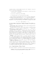
Machines and Contexts
The primary concept in doing formal developments in Event-B is that of a model. A model contains the
complete mathematical development of a Discrete Transition System. It is made of several components
of two kinds: machines and contexts. Machines contain the variables, invariants, theorems, and events
(section 2) of a model, whereas contexts contain carrier sets, constants, axioms, and theorems of a model:
Context
Machine
carrier sets
constants
axioms
theorems
variables
invariants
theorems
events
Machines and contexts have various relationships: a machine can be ”refined” by another one, and a
context can be ”extended” by another one (no cycles are allowed in both these relationships). Moreover, a
machine can ”see” one or several contexts. An example of machine and context relationship is as follows:
sees
Context
Machine
extends
refines
sees
Context
Machine
refines
extends
The following shows a more formal description of machines and contexts:
machine
< machine identif ier >
refines ?
< machine identif ier >
sees ?
< context identif ier >
...
variables
< variable identif ier >
...
invariants
< label >: < predicate >
...
theorems ?
< label >: < predicate >
...
events
< event >
...
variant ?
< variant >
end
context
< context identif ier >
extends ?
< context identif ier >
...
sets ?
< set identif ier >
...
constants ?
< constant identif ier >
...
axioms ?
< label >: < predicate >
...
theorems ?
< label >: < predicate >
...
end
1
In these descriptions, section names (that is, axioms , extends, etc.) followed by a star ? are optional.
Notice that all machine and context identifiers must be distinct in the same model
A model can only contain contexts, or only machines, or both. In the first case, the model represents
a pure mathematical structure. In the third case, the machines of the model are parameterized by the
contexts. Finally, the second case represents a machine which is not parameterized.
Notice that invariants, axioms and theorems denote predicates which are labelled: such labels must be
distinct within a given section. Predicates are defined by means of the Event-B mathematical language
(section 6).
The variant section is explained in section 3.
The previous representation of machines or contexts as well as the usage of keywords do not form a
syntax as there is no such syntax in the Event-B notation. The only part of the Event-B notation which
depends on a well defined syntax is the Event-B mathematical notation (section 6).
2
Events
A machine event represents a transition. It is essentially made of guards and actions (section 4). The
guards together denote the necessary condition for the event to be enabled, whereas the actions together
represent the way the variables of the corresponding machine are modified. Events can have no guards,
they can be also simple and guarded (keyword where) or parameterized and guarded (keywords any and
where). When an event lies in a machine which refines another one then the event may specify (if any)
the abstract event(s) it refines (keyword refines). When a refining event refines an abstract event which
is parameterized, one may provide some witnesses (keyword with), which are presented in section 5. All
this is denoted as follows:
< event identif ier > =
b
status
{normal, convergent, anticipated}
refines ?
< event identif ier >
...
any ?
< parameter identif ier >
...
where ?
< label >: < predicate >
...
with ?
< label >: < witness >
...
then ?
< label >: < action >
...
end
Notice that guards, witnesses, and actions are labelled. As said previously, such labels must be distinct
within a given section.
Most of the time the status section states that the event is ”normal”. A ”convergent” event must be a
new event in a refined machine (one that does not appear in the abstraction). All convergent events in a
2
machine are concerned with the variant section of that machine (see section 3). An ”anticipated” event is
a new event which is not ”convergent” yet but should become ”convergent” in a subsequent refinement.
Notice that a new event might be ”normal”: it means that it is not concerned by the variant section.
This is used quite often when using refinement to add more detail to a specification (without considering
any liveness property of the system).
3
Variant
The variant section appears in a refined machine (section 1) containing some ”convergent” events (section
2). This machine section contains either a natural number expression which must be decreased by each
”convergent” event, or a finite set expression which must be made strictly smaller by each ”convergent”
event.
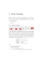
4
Actions
An action can be deterministic, in which case it is made of a list of distinct variable identifiers, followed
by :=, followed by a list of expressions. The latter must be of the same length as the former. Variables
which do not occur in the list are not modified. This is illustrated below:
< variable identif ier list > := < expression list >
Here is an example of a deterministic action in an event situated in machine with variables x. y, and z:
x, y := x + z, y − x
Variables x and y are modified as indicated whereas variable z is not modified.
Alternatively, an action can be non-deterministic, in which case it is made of a list of distinct variable
identifiers, followed by :|, followed by a before-after predicate. Variables which do not occur in the list
are not modified. This is illustrated below:
< variable identif ier list > :| < bef ore af ter predicate >
The before-after predicate may contain all variables of the machine: they denote the corresponding values
just before the action takes place. It can also contain some of the variable identifiers of the list: such
identifiers are primed, they denote the corresponding values just after the action has taken place. Example:
suppose we have three variables x. y and z. Here is a non-deterministic action:
x, y
:|
x0 > y ∧ y 0 > x0 + z
Variable x becomes greater than y and the variable y becomes greater than x0 (the new value for x) added
to z (a variable which is not modified).
A final option is to define a non-deterministic action as a variable identifier (not a list), followed by :∈,
followed by a set expression. This is illustrated below:
3
< variable identif ier > :∈ < set expression >
This form is just a special case of the previous one. It can always be translated to a non-deterministic case
as shown in the following example. Suppose a machine with variables A, x, and y. Here is an action:
x :∈ A ∪ {y}
which is the same as
x :| x0 ∈ A ∪ {y}
Variable x becomes a member of the set A ∪ {y}, whereas variables A and y are not modified.
Finally, notice that all actions in the same event must be concerend with different variables. As an
example, it is not possible to have the following actions in the same event:
x := 5
x :| x0 > x
5
Witnesses
When a concrete event refines an abstract one which is parameterized, then all abstract parameters must
receive a value in the concrete event. Such values are called the witnesses. Each witness is labelled with
the concerned abstract parameter. The witness is defined by a predicate involving the abstract parameter.
Most of the time, this predicate is a simple equality. Next is an example showing two witnesses. On the
left hand side we have an abstract event named pass with two parameters. On the right hand side we have
a concrete event named new pass refining pass
new pass =
b
refines
pass
any
d
where
grd1 : d ∈ ran(dap)
with
p : p = dap−1 (d)
l : l = dst(d)
then
act1 : sit(dap−1 (d)) := dst(d)
act2 : dap := dap − {d}
end
pass =
b
any
p
l
where
grd1 : p 7→ l ∈ aut
grd2 : sit(p) 7→ l ∈ com
then
act1 : sit(p) := l
end
When the concrete event is also parameterized then an abstract parameter which is the same as a concrete need not be given an explicit witness: it is always the corresponding concrete parameter.
6
Syntax of the Event-B Mathematical Notation
It is defined in a separate document entitled ”The Event-B Mathematical Notation”
4
The Event-B Mathematical Language
Christophe Métayer (ClearSy)
Laurent Voisin (ETH Zurich)
October 26, 2007
Contents
1 Introduction
2 Language Lexicon
2.1 Whitespace . . . .
2.2 Identifiers . . . . .
2.3 Integer Literals . .
2.4 Predicate symbols
2.5 Expression symbols
1
.
.
.
.
.
.
.
.
.
.
.
.
.
.
.
.
.
.
.
.
.
.
.
.
.
.
.
.
.
.
.
.
.
.
.
.
.
.
.
.
.
.
.
.
.
.
.
.
.
.
.
.
.
.
.
.
.
.
.
.
.
.
.
.
.
.
.
.
.
.
.
.
.
.
.
.
.
.
.
.
.
.
.
.
.
.
.
.
.
.
2
2
2
3
4
5
3 Language Syntax
3.1 Notation . . . . . . . . . . . . . . .
3.2 Predicates . . . . . . . . . . . . . .
3.2.1 A first attempt . . . . . . .
3.2.2 Associativity of operators .
3.2.3 Priority of operators . . . .
3.2.4 Final syntax for predicates
3.3 Expressions . . . . . . . . . . . . .
3.3.1 Some Fine Points . . . . . .
3.3.2 A First Attempt . . . . . .
3.3.3 Operator Groups . . . . . .
3.3.4 Priority of Operator Groups
3.3.5 Associativity of operators .
3.3.6 Final syntax for expressions
.
.
.
.
.
.
.
.
.
.
.
.
.
.
.
.
.
.
.
.
.
.
.
.
.
.
.
.
.
.
.
.
.
.
.
.
.
.
.
.
.
.
.
.
.
.
.
.
.
.
.
.
.
.
.
.
.
.
.
.
.
.
.
.
.
.
.
.
.
.
.
.
.
.
.
.
.
.
.
.
.
.
.
.
.
.
.
.
.
.
.
.
.
.
.
.
.
.
.
.
.
.
.
.
.
.
.
.
.
.
.
.
.
.
.
.
.
.
.
.
.
.
.
.
.
.
.
.
.
.
.
.
.
.
.
.
.
.
.
.
.
.
.
.
.
.
.
.
.
.
.
.
.
.
.
.
.
.
.
.
.
.
.
.
.
.
.
.
.
.
.
.
.
.
.
.
.
.
.
.
.
.
.
.
.
.
.
.
.
.
.
.
.
.
.
.
.
.
.
.
.
.
.
.
.
.
.
.
.
.
.
.
.
.
.
.
.
.
.
.
.
7
7
7
7
8
9
10
11
11
13
14
16
16
18
4 Static Checking
4.1 Abstract Syntax . . . . . .
4.2 Well-formedness . . . . . .
4.3 Type Checking . . . . . . .
4.3.1 Typing Concepts . .
4.3.2 Specification of Type
4.3.3 Examples . . . . . .
.
.
.
.
.
.
.
.
.
.
.
.
.
.
.
.
.
.
.
.
.
.
.
.
.
.
.
.
.
.
.
.
.
.
.
.
.
.
.
.
.
.
.
.
.
.
.
.
.
.
.
.
.
.
.
.
.
.
.
.
.
.
.
.
.
.
.
.
.
.
.
.
.
.
.
.
.
.
.
.
.
.
.
.
.
.
.
.
.
.
.
.
.
.
.
.
.
.
.
.
.
.
21
21
22
26
26
27
35
.
.
.
.
.
.
.
.
.
.
.
.
.
.
.
.
.
.
.
.
.
.
.
.
.
.
.
.
.
.
.
.
.
.
.
.
.
.
.
.
. . . .
. . . .
. . . .
. . . .
Check
. . . .
5 Dynamic Checking
40
5.1 Predicate Well-Definedness . . . . . . . . . . . . . . . . . . . . . 40
5.2 Expression Well-Definedness . . . . . . . . . . . . . . . . . . . . . 40
i
1
Introduction
This document presents the technical aspects of the kernel mathematical language of event-B. Beyond the pure syntax of the language, it also describes its
lexical structure and various checks (both static and dynamic) that can be done
on formulas on the language.
The main design principle of the language is to have intuitive priorities
for operators and to use a minimal set of parenthesis (except when needed
to resolve common ambiguities). So, the emphasis is really on having formulas
unambiguous and easy to read.
The first chapter describes the lexicon used by the language, then chapter
two describes its (concrete) syntax. Chapter three introduces the notion of wellformed and well-typed formula (static checks). Finally, chapter four gives the
well-definedness conditions for a formula (dynamic check).
Revision History
Contents
Date
2005/05/31
Initial revision (Rodin Deliverable D7).
2006/05/24
Added min and max unary operators.
2007/10/26
Minor corrections in the text.
1
2
Language Lexicon
This chapter describes the lexicon of the mathematical language, that is the
way that terminal tokens of the language grammar are built from a stream of
characters.
Here, we assume that the input stream is made of Unicode characters, as
defined in the Unicode standard 4.0 [4]. As we use only characters of the Basic
Multilingual Plane, all characters are designated by their code points, that is an
uppercase letter ‘U’ followed by a plus sign and an integer value (made of four
hexadecimal digits). For instance, the classical space character is designated by
U+0020.
Each token is formed by considering the longest sequence of characters that
matches one of the definition below.
2.1
Whitespace
Whitespace characters are used to separate tokens or to improve the legibility
of the formula. They are otherwise ignored during lexical analysis.
The whitespace characters of the mathematical language are the Unicode
4.0 space characters:
U+0020
U+2002
U+2008
U+202F
U+00A0
U+2003
U+2009
U+205F
U+1680
U+2004
U+200A
U+3000
U+180E
U+2005
U+200B
U+2000
U+2006
U+2028
U+2001
U+2007
U+2029
together with the following control characters (these are the same as in the Java
Language):
U+0009
U+001C
2.2
U+000A
U+001D
U+000B
U+001E
U+000C
U+001F
U+000D
Identifiers
The identifiers of the mathematical language are defined in the same way as in
the Unicode standard [4, par. 5.15]. This definition is not repeated here. Basically, an identifier is a sequence of characters that enjoy some special property,
like referring to a letter or a digit.
Some identifiers are reserved for the mathematical language, where a predefined meaning is assigned to them. These reserved keywords are the following
2
identifiers made of ASCII letters and digits:
BOOL
bool
inter
prj1
FALSE
card
max
prj2
TRUE
dom
min
ran
finite
mod
succ
id
pred
union
together with those other identifiers that use non-ASCII characters:
2.3
Token
Code points
Token name
N
N1
P
P1
Z
U+2115
U+2115
U+2119
U+2119
U+2124
set of natural numbers
set of positive numbers
powerset
set of non-empty subsets
set of integers
U+0031
U+0031
Integer Literals
Integer literals consists of a non-empty sequence of ASCII decimal digits:
U+0030
U+0035
U+0031
U+0036
U+0032
U+0037
U+0033
U+0038
U+0034
U+0039
Note: There are two ways to tokenize integer literals: either signed or unsigned. The first case as the advantage that it corresponds to classical usage
in mathematics. For instance, the string −1 is thought as representing a number, not a unary minus operator followed by a number. But, as we use the
same character to designate both unary and binary minus, this causes problems: the lexical analysis is no longer context-free, but depends on the syntax
of the language.
There are basically two solutions to this problem. One, taken in some functional languages in the ML family and in the Z notation, is to use different
characters to represent the unary and binary minus operator. However, this
comes against mathematical tradition and is thus rejected. The second solution
is to consider that integer literals are unsigned. This second solution has been
chosen here.
3
2.4
Predicate symbols
The tokens used in the pure predicate calculus are:
Token
Code point
(
)
⇔
⇒
∧
∨
¬
>
⊥
∀
∃
,
·
U+0028
U+0029
U+21D4
U+21D2
U+2227
U+2228
U+00AC
U+22A4
U+22A5
U+2200
U+2203
U+002C
U+00B7
Token name
left parenthesis
right parenthesis
logical equivalence
logical implication
logical and
logical or
not sign
true predicate
false predicate
for all
there exists
comma
middle dot
The symbolic tokens used to build predicates from expressions are:
Token
Code point
=
6
=
<
≤
>
≥
∈
∈
/
⊂
6
⊂
⊆
6
⊆
U+003D
U+2260
U+003C
U+2264
U+003E
U+2265
U+2208
U+2209
U+2282
U+2284
U+2286
U+2288
Token name
equals sign
not equal to
less-than sign
less than or equal to
greater-than sign
greater than or equal to
element of
not an element of
subset of
not a subset of
subset of or equal to
neither a subset of nor equal to
4
2.5
Expression symbols
The following symbolic tokens are used to build sets of relations (or functions):
Token
Code point
↔
←
↔
↔
→
↔
↔
→
7
→
7
7
U+2194
U+E100
U+E101
U+E102
U+21F8
U+2192
U+2914
U+21A3
U+2900
U+21A0
U+2916
Token name
relation
total relation
surjective relation
total surjective relation
partial function
total function
partial injection
total injection
partial surjection
total surjection
bijection
The following symbolic tokens are used for manipulating sets:
Token
Code point
{
}
7
→
∅
∩
∪
\
×
U+007B
U+007D
U+21A6
U+2205
U+2229
U+222A
U+2216
U+00D7
Token name
left curly bracket
right curly bracket
maplet
empty set
intersection
union
set minus
cartesian product
The following symbolic tokens are used for manipulating relations and functions:
Token
Code point
Token name
[
]
7
→
C
−
◦
;
⊗
k
−1
C
−
C
B
−
B
U+005B
U+005D
U+21A6
U+E103
U+2218
U+003B
U+2297
U+2225
U+223C
U+25C1
U+2A64
U+25B7
U+2A65
left square bracket
right square bracket
maplet
relation overriding
backward composition
forward composition
direct product
parallel product
tilde operator
domain restriction
domain subtraction
range restriction
range subtraction
5
The following symbolic tokens are used in quantified expressions:
Token
Code point
λ
T
S
U+03BB
U+22C2
U+22C3
U+2223
|
Token name
lambda
n-ary intersection
n-ary union
such that
The following symbolic tokens are used in arithmetic expressions:
Token
Code point
..
+
−
∗
÷
b
U+2025
U+002B
U+2212
U+2217
U+00F7
U+005E
Token name
upto operator
plus sign
minus sign
asterisk operator
division sign
exponentiation sign
6
3
Language Syntax
This chapter describes the syntax of the mathematical language, giving the
rationale behind the design decisions made.
We first present the notation we use to describe the syntax of the mathematical language. Then, we present the syntax of predicates and of expressions.
In each case, we first present a simple ambiguous grammar, then we tackle with
associativity and priorities of operators, giving a rationale for each choice made.
Finally, we give a complete and non-ambiguous syntax.
3.1
Notation
In this document, we use an Extended Backus-Naur Form (EBNF) to describe
syntax. In that notation, non-terminals are surrounded by angle brackets and
terminals surrounded by single quotes. The other symbols are meta-symbols:
• Symbol ::= defines the non-terminal appearing on its left in terms of the
syntax on its right.
• Parenthesis ( and ) are used for grouping.
• A vertical bar | denotes alternation.
• Square brackets [ and ] surround an optional part.
• Curly brackets { and } surround a part that can be repeated zero or more
times.
3.2
Predicates
The point here is to define a grammar which is quite similar to the one used
commonly when writing mathematical formulae but that should also be nonambiguous to the (human) reader.
3.2.1
A first attempt
The grammar commonly used for predicates can loosely be defined as follows:
hpredicatei ::=
|
|
|
‘(’ hpredicatei ‘)’
hpredicatei ‘⇔’ hpredicatei
hpredicatei ‘⇒’ hpredicatei
hpredicatei ‘∧’ hpredicatei
7
|
|
|
|
|
|
|
|
|
|
|
hpredicatei ‘∨’ hpredicatei
‘¬’ hpredicatei
‘>’
‘⊥’
‘∀’ hident-listi ‘·’ hpredicatei
‘∃’ hident-listi ‘·’ hpredicatei
‘finite’ ‘(’ hexpressioni ‘)’
hexpressioni ‘=’ hexpressioni
hexpressioni ‘∈’ hexpressioni
hexpressioni ‘≤’ hexpressioni
...
hident-listi ::= hident-listi ‘,’ hidenti
| hidenti
The ellipsis which appears at the end of the hpredicatei production rule
means that there are still more alternatives combining two expressions into a
predicate. All those alternatives are not really relevant at this point of the document, but will be fully listed in the final syntax (see section 3.2.4 on page 10).
3.2.2
Associativity of operators
In this document, we use the term associativity with somewhat two different
meanings. In a mathematical context, when we write that an operator, say ◦, is
associative, we mean that it has a special mathematical property, namely that
(x ◦ y) ◦ z has the same value as x ◦ (y ◦ z). In a syntactical context, we say that
an operator is left-associative when formula x ◦ y ◦ z (without any parenthesis)
is parsed as if it would have been written (x ◦ y) ◦ z. To avoid any ambiguity,
we will always write associative in the algebraic sense when we refer to the first
meaning, the bare word associative always having the syntactical meaning.
Getting back to our predicate grammar defined above, we see that it is
somewhat ambiguous. A first point is that it doesn’t specify how one should
parse formulae containing twice the same binary predicate operator without any
parenthesis such as
P ⇒Q⇒R
P ∧Q∧R
To solve that ambiguity, one specifies that each binary operator has a property called associativity. The associativities defined for the event-B language
are the following:
Operator
Associativity
⇔
none
⇒
none
∧
left
∨
left
8
Caution
As a consequence, formula P ⇒ Q ⇒ R is considered as ill-formed and not
part of the event-B language, whereas formula P ∧ Q ∧ R will be parsed as if it
actually were written as (P ∧ Q) ∧ R.
The rationale for these associativities is quite simple. Operator ∧ is associative in the algebraic sense, so formulae (P ∧ Q) ∧ R and P ∧ (Q ∧ R) have the
same meaning. Hence, one can pick up either left or right associativity for this
operator. We arbitrarily chose left associativity as it is the most commonly used
to our knowledge. The same rationale explains the choice of left associativity
for operator ∨.
On the other hand, operator ⇒ is not associative in the algebraic sense
(P ⇒ Q) ⇒ R is not the same as P ⇒ (Q ⇒ R) (just suppose that predicates
P , Q and R are all ⊥). As a consequence, we keep it non associative in the
language, rather than choosing an arbitrary associativity.
The case of operator ⇔ is somewhat special. This operator is indeed associative in the algebraic sense. However, mathematicians often write formula
P ⇔ Q ⇔ R when they actually mean (P ⇔ Q) ∧ (Q ⇔ R). Hence, we chose
to make that operator non associative in the event-B language to avoid any
ambiguity.
Finally, for the operators that build a predicate from two expressions (such
as =, ∈, etc.), the grammar given above doesn’t allow formulae like x = y = z,
so those operator can not be associative.
3.2.3
Priority of operators
Another source of ambiguity is the case where formulae contain two different
predicate operators without any parenthesis such as
P ⇒Q⇔R
P ∧Q∨R
¬P ∧ Q
∀x·P ∨ Q
This kind of ambiguity is generally resolved by defining priorities among
operators which define how much binding power each operator has. We will
use that mechanism here, retaining the most commonly used priorities. But,
with the addition that we want to forbid cases where those priorities are not so
well-accepted.
For instance, some people expect operators ‘∧’ and ‘∨’ to have the same
priority, while others expect operator ‘∧’ to have higher priority. So when faced
with formula P ∨ Q ∧ R, some people read it as (P ∨ Q) ∧ R while others read
it as P ∨ (Q ∧ R), which is quite different (just replace P and Q by > and R by
⊥ to convince yourself).
To solve that ambiguity, we decided that operators ‘∧’ and ‘∨’ indeed have
the same priority, but that one cannot mix them together without using parenthesis. So, P ∧Q∨R is considered ill-formed. One should write either (P ∧Q)∨R
or P ∧ (Q ∨ R).
The priorities defined for the event-B language are the following (from lower
9
to higher priority)
∀x·P and ∃x·P
(mixing allowed)
P ⇒ Q and P ⇔ Q (mixing not allowed)
P ∧ Q and P ∨ Q (mixing not allowed)
¬P
We choose to give quantified predicates the lowest priority in order to ease
their reading when embedded in long formulae. The main consequence of this
choice is that the scope of the variables introduced by a quantifier is the longest
sub-formula. For instance, in formula (∀x·P ⇒ Q) ⇒ R, the scope of variable x
extends until predicate Q as can be easily seen by looking at matching parenthesis.
The following formulae show some examples of how those priorities are used
to replace parenthesis in some common cases:
P ∧Q⇒R
is parsed as
(P ∧ Q) ⇒ R
∀x·∃y·P
is parsed as
∀x·(∃y·P )
∀x·P ⇒ Q is parsed as
∀x·(P ⇒ Q)
∀x·P ∧ Q is parsed as
∀x·(P ∧ Q)
∀x·¬P
is parsed as
∀x·(¬P )
¬P ⇒ Q is parsed as
(¬P ) ⇒ Q
¬P ∧ Q is parsed as
(¬P ) ∧ Q
One should notice the difference with classical B [1] where ∀x·P ⇒ Q is
parsed as (∀x·P ) ⇒ Q whereas, again, it is parsed here as ∀x·(P ⇒ Q).
3.2.4
Final syntax for predicates
As a result, we obtain the following non ambiguous grammar for predicates:
hpredicatei
::= { hquantifier i } hunquantified-predicatei
hquantifier i
::= ‘∀’ hident-listi ‘·’
| ‘∃’ hident-listi ‘·’
hident-listi
::= hidenti { ‘,’ hidenti }
hunquantified-predicatei ::= hsimple-predicatei [ ‘⇒’ hsimple-predicatei ]
| hsimple-predicatei [ ‘⇔’ hsimple-predicatei ]
hsimple-predicatei
::= hliteral-predicatei { ‘∧’ hliteral-predicatei }
| hliteral-predicatei { ‘∨’ hliteral-predicatei }
hliteral-predicatei
::= { ‘¬’ } hatomic-predicatei
10
hatomic-predicatei
::=
|
|
|
|
hrelopi
::= ‘=’ | ‘6=’
| ‘∈’ | ‘∈’
/ | ‘⊂’ | ‘6⊂’ | ‘⊆’ | ‘6⊆’
| ‘<’ | ‘≤’ | ‘>’ | ‘≥’
‘⊥’
‘>’
‘finite’ ‘(’ hexpressioni ‘)’
hpair-expressioni hrelopi hpair-expressioni
‘(’ hpredicatei ‘)’
Please note that for relational predicates, we are using ¡pair-expression¿
instead of ¡expression¿. That change will only allow expressions without quantifiers on each side of the relational operator. As a consequence, when one wants
to use a quantified expression on either side, one will have to surround it with
parenthesis. For instance, predicate λx·x ∈ Z | x = id(Z) is not well-formed,
one must write instead (λx·x ∈ Z | x) = id(Z).
3.3
Expressions
The design principle for the syntax of expressions is the same as that of predicates, namely to enhance readability. To fulfill this goal, we use the same
techniques: minimize the need for parenthesis where they are not really needed
and prevent mixing operators when such a mix would be ambiguous.
3.3.1
Some Fine Points
Before presenting a first attempt of the syntax of expressions, we shall study
some fine points about pairs, set comprehension, lambda abstraction, quantified
expressions, and first and second projections.
Pair Construction. Pairs of expressions are constructed using the maplet
operator ‘7→’. Contrary to classical B [1], it is not possible to use a comma
anymore. This change is due to the ambiguity of using commas for two different
purposes in classical B: as a pair constructor and as a separator. For instance, set
{1, 2} can be seen as either a set containing the pair (1, 2) or as a set containing
the two elements 1 and 2. That was very confusing.
In event-B, a comma is always a separator and a maplet is a pair constructor.
Below are some examples showing the consequences of this new approach:
Classical-B Event-B
x, y ∈ S
x 7→ y ∈ S
x, y = z, t
x 7→ y = z 7→ t
f (x, y)
f (x 7→ y)
The last example is particularly blatant of the confusion between separator
and pair constructor in classical B. When looking at formula f (x, y), one has
the impression that function f takes two separate arguments. But, this is not
always true. For instance, variable x could hide a non scalar value. For instance,
11
suppose that x = a 7→ b, then the function application could be rewritten as
either f (a 7→ b, y) or even as f (a, b, y). In that latter case, function f now
appears to take three arguments. This is clearly not satisfactory. In fact,
function f only takes one argument, which can happen to be a pair. In that
latter case, one should use a pair constructor to create that pair, that is use a
maplet operator.
Set Comprehension. There are now two forms of set comprehension. The
most general one is {x · P (x) | E(x)} which describes the set whose elements
are E(x), for all x such that P (x) holds. For instance, the set of all even natural
numbers can be written as {x · x ∈ N | 2 ∗ x}.
The second form {E | P } is just a short-hand for the first-one, which allows
to write things more compactly. The difference from the first form is that
the variables that are bound by the construct are not listed explicitly. They
are inferred from the expression part. Continuing with our previous example,
the set of all even natural numbers can then be written more compactly as
{2 ∗ x | x ∈ N}, which corresponds more to the classical mathematical notation.
The rule for determining the variables which are bound by this second form
is to take all variables that occur free in E. Thus, if we denote by x the list of the
variables that occur free in E, then the second form is equivalent to {x · P | E}.
Lambda Abstraction. For lambda abstraction, classical B [1] uses the form
(λx · P | E) where x is a list of variables, P a predicate and E an expression.
This notation is fine when x is reduced to only one variable. For instance,
expression (λx · x ∈ N | x + 1) denotes the classical succesor function on
natural numbers. It is equal by definition to the set {x · x ∈ N | x + 1}.
But things get more complicated when x represents more than one variable.
For instance, what is the meaning of expression (λa, b · P | E). In classical B,
the latter expression is defined as being the set {a, b · P | a 7→ b 7→ E}. This is
clearly unsatisfactory for event-B, as it turns out that, in the former expression,
the comma that appears between a and b is not only a separator between two
variables, but also a hidden pair constructor, as one can see when writing the
equivalent set comprehension.
The crux of the matter is that the list of variables x introduced above, is
much more than a simple list. Indeed, it describes the structure of the domain of
the function defined by the lambda abstraction. For instance, when one writes,
in classical B, the expression (λa, b · P | E), one means that the domain of
that function is A × B (where A and B are the types of bound variables a and
b). Hence, the use of a comma is not appropriate here, as advocated in the
paragraph above about Pair Construction.
The cure is easy, just say that x is not a list of variables, but a pattern that
specifies the structure of the domain of the lambda abstraction. The example
above is then to be written as (λa 7→ b · P | E). Moreover, this can be
generalized to arbitrary domain structure by allowing arbitrary patterns after
the lambda operator. The only constraints are that those patterns should be
constructed out of distinct variables, pair constructors and parenthesis. The
definition of the lambda abstraction (λx · P | E) becomes {X · P | x 7→ E}
where X is the list of the variables that occur in x.
12
Other Quantified Expressions. The other quantified expressions are the
quantified union and intersection. In this paragraph, we shall only consider
quantified intersection, but everything will also apply to quantified union, mutatis mutandis.
T
A quantified intersection expression has the form ( x · P | E) where x is a
list of variables, P a predicate and E an expression. It’s defined as being a short
form for the equivalent expression inter({x · P | E}) which mixes generalized
intersection and set comprehension. But, as we have seen above, we also have a
short form for writing set comprehension. The question then arises whether we
could also define a short form for generalized
intersection. The answer is yes.
T
We then have a second form which is ( E | P ) and which is defined has being
equal to inter({E | P }).
Projections. In classical B [1], the first and second projection operators take
two sets as arguments, like for instance in the expression prj1 (A, B). In that
expression, arguments A and B are used for two different purposes. On the one
end, they allow to infer the type associated to the instantiated operator. On
the other hand, they define the domain of the instantiated operator, which is
A × B.
This approach seems unnecessarily restrictive, as it puts a strong constraint
on the domain of the operator, namely that it must be a cartesian product.
So, in event-B, these operators become unary and take a relation as argument.
The argument is then their domain. The upgrade path from classical B is quite
straightforward, just replace prj1 (A, B) by prj1 (A × B).
3.3.2
A First Attempt
An ambiguous grammar for event-B expressions can loosely be defined as follows:
hexpressioni
::=
|
|
|
|
|
|
|
|
|
|
|
|
|
|
|
|
|
hexpressioni hbinary-operator i hexpressioni
hunary-operator i hexpressioni
hexpressioni ‘−1 ’
hexpressioni ‘[’ hexpressioni ‘]’
hexpressioni ‘(’ hexpressioni ‘)’
‘λ’ hident-patterni ‘·’ hpredicatei ‘|’ hexpressioni
hquantifier i hident-listi ‘·’ hpredicatei ‘|’ hexpressioni
hquantifier i hexpressioni ‘|’ hpredicatei
‘{’ hident-listi ‘·’ hpredicatei ‘|’ hexpressioni ‘}’
‘{’ hexpressioni ‘|’ hpredicatei ‘}’
‘bool’ ‘(’ hpredicatei ‘)’
‘{’ [ hexpression-listi ] ‘}’
‘(’ hexpressioni ‘)’
‘∅’
‘Z’ | ‘N’ | ‘N1 ’
‘BOOL’ | ‘TRUE’ | ‘FALSE’
hidenti
hinteger-literal i
13
hbinary-operator i ::= ‘7→’ | ‘↔’ | ‘←
↔’ | ‘↔
→’ | ‘↔
↔’ | ‘→’
7 | ‘→’ | ‘’
7 | ‘’ | ‘’
7
| ‘’ | ‘
’ | ‘∪’ | ‘∩’ | ‘\’ | ‘×’ | ‘⊗’ | ‘k’ | ‘◦’ | ‘;’ | ‘C
−’ |
‘C’ | ‘C
−’ | ‘B’ | ‘B
−’ | ‘..’ | ‘+’ | ‘−’ | ‘∗’ | ‘÷’ | ‘mod’ | ‘b’
hunary-operator i ::= ‘−’ | ‘card’ | ‘P’ | ‘P1 ’ | ‘union’ | ‘inter’ | ‘dom’ | ‘ran’ |
‘prj1 ’ | ‘prj2 ’ | ‘id’ | ‘min’ | ‘max’
hquantifier i
S
T
::= ‘ ’ | ‘ ’
hident-patterni ::= hident-patterni ‘7→’ hident-patterni
| ‘(’ hident-patterni ‘)’
| hidenti
hexpression-listi ::= hexpression-listi ‘,’ hexpressioni
| hexpressioni
As can be seen, there are many expression operators in the event-B language.
So, we’ll need to take a divide and conquer approach: to make things easier to
grasp, we will first try to group all those operators into some categories.
3.3.3
Operator Groups
Basically, there are several kinds of expressions. The most important ones are
shown in Figure 3.1. This figure reads as follows: there are three top-level kinds
of expressions: sets, pairs and scalars. Relations and sets of relations are some
special kinds of set. For instance, a relation between a set A and a set B is
a subset of A × B. The set of all relations between A and B is the set of all
subsets of A × B. Integers and booleans are also some special kind of scalar
expression.
expression
set
relation
pair
set of relations
scalar
integer
boolean
Figure 3.1: Kinds of expressions
We now define groups of similar expression operators (see Table 3.1 on the
following page). The groups are defined by considering the shape of the operator
(binary, unary, quantified, etc.) but also the kind of operator arguments and
result. For each group, we will give one operator which will be used in the sequel
as a distinguished representative of its group.
When examining that table, we can remark an interesting point: the operators that belong to the last three groups have the special property of being
14
Group
Description
Repr.
Quantification
operators
Given a list of quantified identifiers,
a predicate and an expression, these
operators produce a new expression.
λx·P | E
Pair constructor
Given two expressions, it produces a
pair.
E 7→ F
Set of relations
constructors
Given two sets, these operators produce a set of relations.
S→
7 T
Binary set
operators
Given two sets, these operators produce a new set.
S∪T
Interval constructor
Given two integers, this operator
produces a set.
i .. j
Arithmetic
operators
Given one or two integers, these operators produce a new integer.
i+j
Relational and
functional image
Given a relation and an expression,
these operators produce a new expression.
r[s]
Unary relation
operator
Given a relation, this operator produces a new relation.
r−1
Tightly bound
unary operators
Given an expression, these operators
produce another expression.
P(S)
Predicate
conversion
Given a predicate, this operator produces a new boolean expression.
bool(P )
Set enumeration
and comprehension
Given a list of expressions, or a list
of quantified variables, a predicate
and an expression, this operator produces a set.
{. . .}
Table 3.1: Groups of similar expression operators
15
bounded: when one encounters such an operator, one can find easily where the
expression involving that operator starts and where it ends: unary and ‘bool’
operators are always followed by a formula enclosed within parenthesis; set enumerations and comprehensions are enclosed within curly brackets. This is also
the case of atomic expressions like integer and boolean literals or identifiers.
On the other hand, the operators of the other groups are not bounded by
themselves, so one needs to define priorities and associativity laws for them in
order to resolve potential ambiguities. We will first start by defining priorities
between groups, then we will refine each group separately.
3.3.4
Priority of Operator Groups
We arbitrarily choose to define relative priorities such that groups of operators are sorted by increasing priority in table 3.1 on the previous page. As a
consequence, quantification operators have the lowest priority.
That order has been chosen because it reduces the number of needed parenthesis when writing most common expressions. Here are a few example to
illustrate this. Each expression is stated twice, first without parenthesis, then
fully parenthesized:
A ∪ B 7→ C
is parsed as
(A ∪ B) 7→ C
a + b 7→ c is parsed as
(a + b) 7→ c
a .. b ∪ C
is parsed as
(a .. b) ∪ C
a + b .. c is parsed as
(a + b) .. c
r
−1
∪ s is parsed as
r−1 (s)
is parsed as
(r−1 ) ∪ s
(r−1 )(s)
Also, we give the lowest priority to quantification operators so that, when
embedded in a formula, they have to be written surrounded by parenthesis.
This is consistent with the choice made for quantified predicates. An example
formula is
(λx·x ∈ Z | x + 1)−1 (3) = 2
3.3.5
Associativity of operators
Now, that priorities of groups have been defined, we will resolve remaining
ambiguities separately for each group, defining how operators of each group can
be mixed.
Quantification Operators. In this group, there is not much room for ambiguity, as when we encounter two quantification operators, it comes right from
their syntax that the second one will be embedded in the first one. The only option left is whether the second quantified expression should be enclosed within
parenthesis or not. We decide not to enforce parenthesis in this case. As a
consequence, formula
\
x · x ⊆ Z | λy·y = x | y ∪ {0}
16
is parsed as
\
x · x ⊆ Z | (λy·y = x | y ∪ {0}) .
Pair Constructor. This group contains only the maplet operator, so we only
have to define an associativity property for that operator. Although the maplet
operator is not associative in the algebraic sense, it is very common usage to
parse it as left-associative, so we shall keep that property. Then, an expression
of the form a 7→ b 7→ c will be parsed as (a 7→ b) 7→ c.
Set of Relations Constructors. No operator in this group is associative
in the algebraic sense. However, we decide to parse them as right-associative.
That choice is justified by the fact that we will parse function application as
left-associative (this will be stated when we reach the Relational and functional
image paragraph on the following page). As a consequence, one can write
f (a)(b) when one actually means (f (a))(b). Then, to be consistent, one should
also be able to describe properties of function f without parenthesis, so formula
f ∈A→
7 B→
7 C should be parsed as f ∈ A →
7 (B →
7 C).
Binary Set Operators. This group contains various operators which are
more or less compatible each with the other. So, let’s first see how one can
safely mix these operators in a formula, from a mathematical point of view.
Table 3.2 on the next page shows operator compatibility. We write a cross at
the intersection of a row and a column if the two operators are compatible in
the following sense: operator oprow is compatible with operator opcol if and only
if the following equality holds
(A oprow B) opcol C = A oprow (B opcol C).
For instance, the cross at the intersection of row two and column three tells us
that (A ∩ B) \ C = A ∩ (B \ C) and the cross at the intersection of row nine
and column seven tells us that (A C r) ⊗ s = A C (r ⊗ s).
We can see that the shape is quite irregular and that there are not so many
cases where operators are compatible. So, to have an unambiguous language,
we should stick to that compatibility relation and forbid any unparenthesized
combination of incompatible operators. When two operators are compatible,
we parse them as left-associative. Otherwise, one needs to use parenthesis to
resolve ambiguities. For instance, formula S ∪ T ∪ U is parsed as (S ∪ T ) ∪ U ,
while formula S ∪ T ∩ U is ill-formed and is rejected. One has to make precise
the meaning of that last formula, writing either (S ∪ T ) ∩ U or S ∪ (T ∩ U ).
There is only one case where we want to allow the combination of two incompatible operators: we parse the cartesian product operator as left-associative.
This exception to the above rule is justified by the fact that we want to be
consistent with the left-associativity we have given to the maplet operator.
Then, one can write a 7→ b 7→ c ∈ A × B × C when one actually means
(a 7→ b) 7→ c ∈ (A × B) × C.
Interval Constructor. This group contains only one operator: ‘..’. There is
no point in having this operator used twice in the same formula (which would
give the nonsensical formula a .. b .. c). So, this operator is parsed as nonassociative.
17
∪
∩
\
×
◦
;
⊗
k
C
−
C
−
C
B
−
B
∪
×
∩
\
×
×
×
◦
⊗
;
k C
− C −
C B −
B
×
×
×
×
×
×
×
×
×
×
×
×
×
×
×
×
×
×
×
Table 3.2: Compatibility of binary set operators
Arithmetic Operators. For these operators, we choose to retain the Ada
language specification for defining priorities and associativity: operators ‘+’ and
‘−’ both have the same priority and are parsed as left-associative, operators ‘∗’,
‘÷’ and ‘mod’ have higher priority and are also parsed as left-associative. Note
that this choice is different from the one made for instance in the C language,
where there is a special priority for unary ‘−’. We did not retain that last point
as it can lead to valid but hard to read expressions like a + − − − − b which
means a + b.
Finally, the exponentiation operator has the least priority and is parsed as
non-associative.
Relational and Functional Image. We choose to make these operations
left-associative, although they are not associative in the algebraic sense. This
follows common usage and is indeed important to have easy to read formulas.
If these operators were not associative, one would have to write quite intricate
formulas just to express successive function application: ((f (a))(b))(c). With
the left-associativity we’ve added, this becomes f (a)(b)(c).
Unary Relation Operator. This group contains only one operator ‘−1 ’,
which can be repeated, obviously, so that r−1−1 is parsed as (r−1 )−1 .
3.3.6
Final syntax for expressions
As a result, we obtain the following non ambiguous grammar for expressions. An
important point is that non-terminals are named after the group of the top-level
operators appearing in their production rule. This can be somewhat misleading
as, for instance, hpair-expressioni can be derived as formula Z, which is clearly
not a pair. This naming policy was chosen not to leave any information (just
18
numbering non-terminals 1, 2,. . . would miss some structural property of the
grammar).
hexpressioni
::=
|
|
|
|
|
‘λ’
S hident-patterni ‘·’ hpredicatei ‘|’ hexpressioni
‘S’ hident-listi ‘·’ hpredicatei ‘|’ hexpressioni
‘T’ hexpressioni ‘|’ hpredicatei
‘T’ hident-listi ‘·’ hpredicatei ‘|’ hexpressioni
‘ ’ hexpressioni ‘|’ hpredicatei
hpair-expressioni
hident-patterni
::= hident-patterni { ‘7→’ hident-patterni }
| ‘(’ hident-patterni ‘)’
| hidenti
hpair-expressioni
::= hrelation-set-expr i { ‘7→’ hrelation-set-expr i }
hrelation-set-expr i
::= hset-expr i { hrelational-set-opi hset-expr i }
hrelational-set-opi
::= ‘↔’ | ‘←
↔’ | ‘↔
→’ | ‘↔
↔’
| ‘→’
7 | ‘→’ | ‘’
7 | ‘’ | ‘’
7 | ‘’ | ‘
’
hset-expr i
::=
|
|
|
|
|
hdomain-modifier i
::= hinterval-expr i ( ‘C’ | ‘C
−’ )
hrelation-expr i
::= hinterval-expr i ‘⊗’ hinterval-expr i
| hinterval-expr i { ‘;’ hinterval-expr i }
[ hrange-modifier i ]
| hinterval-expr i { ‘∩’ hinterval-expr i }
[ ‘\’ hinterval-expr i | hrange-modifier i ]
hrange-modifier i
::= ( ‘B’ | ‘B
−’ ) hinterval-expr i
hinterval-expr i
::= harithmetic-expr i [ ‘..’ harithmetic-expr i ]
harithmetic-expr i
::= [ ‘−’ ] htermi { ( ‘+’ | ‘−’ ) htermi }
htermi
::= hfactor i { ( ‘∗’ | ‘÷’ | ‘mod’ ) hfactor i }
hfactor i
::= himagei [ ‘b’ himagei ]
himagei
::= hprimaryi { ‘[’ hexpressioni ‘]’ | ‘(’ hexpressioni ‘)’ }
hprimaryi
::= hsimple-expr i { ‘−1 ’ }
hinterval-expr i { ‘∪’ hinterval-expr i }
hinterval-expr i { ‘×’ hinterval-expr i }
hinterval-expr i { ‘C
−’ hinterval-expr i }
hinterval-expr i { ‘◦’ hinterval-expr i }
hinterval-expr i ‘k’ hinterval-expr i
[ hdomain-modifier i ] hrelation-expr i
19
hsimple-expr i
::=
|
|
|
|
|
|
|
|
‘bool’ ‘(’ hpredicatei ‘)’
hunary-opi ‘(’ hexpressioni ‘)’
‘(’ hexpressioni ‘)’
‘{’ hident-listi ‘·’ hpredicatei ‘|’ hexpressioni ‘}’
‘{’ hexpressioni ‘|’ hpredicatei ‘}’
‘{’ [ hexpressioni { ‘,’ hexpressioni } ] ‘}’
‘Z’ | ‘N’ | ‘N1 ’ | ‘BOOL’ | ‘TRUE’ | ‘FALSE’ | ‘∅’
hidenti
hinteger-literal i
hunary-opi
::= ‘card’ | ‘P’ | ‘P1 ’ | ‘union’ | ‘inter’ | ‘dom’ | ‘ran’ | ‘prj1 ’
| ‘prj2 ’ | ‘id’ | ‘min’ | ‘max’
20
4
Static Checking
This chapter describes how mathematical formulae (predicates and expressions)
are to be statically checked for being meaningful. We first describe an abstract
syntax for formulae. Then, we state the static checks that are to be done, based
on that abstract syntax:
• well-formedness,
• type-check.
4.1
Abstract Syntax
In this section, we specify an abstract syntax for mathematical formulae. This
abstract syntax is based on the concrete syntax described in Section 3.2.4 on
page 10 and Section 3.3.6 on page 18. The difference is that the abstract syntax
only conserves the essence of the concrete syntax. So, all concrete matter like
priorities and tokens do not appear anymore.
The abstract syntax is described using production rules. Each rule has its
own label. It is made of a left-hand part which denotes some kind of formula
(predicate, expression, identifier list, expression list) and a right hand part which
denotes a list of sub-formulae together with some attributes. To distinguish an
attribute from a sub-formulae, we enclose the former within square brackets.
Moreover, to make rules short, we use single letters, possibly subscripted, to
denote formulae: a P denotes a predicate, E an expression, L a list of identifiers,
I an identifier, M a list of expressions, and Q a pattern for lambda abstraction.
The production rules for predicates are:
pred-bin:
pred-una:
pred-quant:
pred-lit:
pred-simp:
pred-rel:
P
P
P
P
P
P
::=
::=
::=
::=
::=
::=
P1 P2 [pred-binop]
P1
L1 P1 [pred-quant]
[pred-lit]
E1
E1 E2 [pred-relop]
where
pred-binop ∈ {land, lor, limp, leqv}
pred-quant ∈ {forall, exists}
pred-lit ∈ {btrue,
bfalse}
equal, notequal, lt, le, gt, ge,
pred-relop ∈
.
in, notin, subset, notsubset, subseteq, notsubseteq
21
The production rules for lists of identifiers and identifiers are:
ident-list: L ::= I1 I2 . . . In
ident: I ::= [name]
where
1≤n
name is a string of characters.
The production rules for expressions are:
expr-bin:
expr-una:
expr-lambda:
expr-quant1:
expr-quant2:
expr-bool:
expr-eset:
expr-ident:
expr-atom:
expr-int:
E
E
E
E
E
E
E
E
E
E
::=
::=
::=
::=
::=
::=
::=
::=
::=
::=
E1 E2 [expr-binop]
E1 [expr-unop]
Q1 P1 E1
L1 P1 E1 [expr-quant]
E1 P1 [expr-quant]
P1
M1
I1
[expr-lit]
[int-lit]
pattern: Q ::= Q1 Q2
pattern-ident: Q ::= I1
expr-list: M ::= E1 E2 . . . En
where

funimage, relimage, mapsto,




rel,
trel, srel, strel,



pfun, tfun, pinj, tinj, psur, tsur, tbij,
expr-binop ∈
bunion, binter, setminus, cprod, dprod, pprod,




bcomp, fcomp, ovl, domres, domsub, ranres, ransub,



upto,
plus, minus, mul, div, mod, expn
uminus, converse, card, pow, pow1,
expr-unop ∈
union, inter, dom, ran, prj1, prj2, id, min, max
expr-quant ∈ {qunion, qinter, cset}
expr-lit ∈ {integer, natural, natural1, bool, true, false, emptyset}
int-lit is an integer number.
4.2















Well-formedness
Each occurrence of an identifier in a formula (that is a predicate or an expression) can be either free or bound. Intuitively, a free occurrence of an identifier
refers to a declaration of that identifier in a scope outside of the formula, while a
bound occurrence corresponds to a local declaration introduced by a quantifier
in the formula itself.
For a formula to be considered well-formed, we ask that, beyond being syntactically correct, it also satisfies the two following conditions:
1. Any identifier that occurs in the formula, should have only free occurrences
or bound occurrences, but not both.
22
2. Any identifier that occurs bound in the formula, should be bound in exactly one place (i.e., by only one quantifier).
These conditions have been coined so that any occurrence of an identifier in
a formula always denotes exactly the same data. This is a big win in formula
legibility.
For instance, the following formula is ill-formed (it doesn’t satisfy the first
condition)
(λx·x ∈ Z | x + 1) (x) = x + 1
it should be written
(λy·y ∈ Z | y + 1) (x) = x + 1 .
And the following formula is also ill-formed (failing to satisfy the second
condition)
(λx·x ∈ Z | x + 1) = (λx·x ∈ Z | x + 1)
it should be written
(λx·x ∈ Z | x + 1) = (λy·y ∈ Z | y + 1) .
The rest of this section formalizes these well-formedness conditions using an
attribute grammar formalism on the abstract syntax of formulae. For that, we
add three attributes to the nodes of the abstract syntax tree:
• Attribute bound is synthesized and contains the set of identifiers that occur
bound in the formula rooted at the current node.
• Attribute free is synthesized and contains the set of identifiers that occur
free in the formula rooted at the current node.
• Attribute wff is synthesized and contains a boolean value which is TRUE
if and only if the formula rooted at the current node is well-formed.
The value of these three attributes are given by the following set of equations
on the production rules of the abstract syntax:
pred-bin: P ::= P1 P2 [pred-binop]
P.bound = P1 .bound ∪ P2 .bound
P.free = P1 .free
 ∪ P2 .free
P1 .wff = TRUE
 ∧ P2 .wff = TRUE

P.wff = bool 
 ∧ P1 .free ∩ P2 .bound = ∅
 ∧ P1 .bound ∩ P2 .free = ∅
∧ P1 .bound ∩ P2 .bound = ∅
pred-una: P ::= P1
P.bound = P1 .bound
P.free = P1 .free
P.wff = P1 .wff
23






pred-quant: P ::= L1 P1 [pred-quant]
P.bound = P1 .bound ∪ L1 .free
P.free = P1 .free
 \ L1 .free

L1 .wff = TRUE

P.wff = bool  ∧ P1 .wff = TRUE
∧ P1 .bound ∩ L1 .free = ∅
pred-lit: P ::= [pred-lit]
P.bound = ∅
P.free = ∅
P.wff = TRUE
pred-simp: P
P.bound
P.free
P.wff
::= E1
= E1 .bound
= E1 .free
= E1 .wff
pred-rel: P ::= E1 E2 [pred-relop]
P.bound = E1 .bound ∪ E2 .bound
P.free = E1 .free
 ∪ E2 .free
E1 .wff = TRUE
 ∧ E2 .wff = TRUE

P.wff = bool 
 ∧ E1 .free ∩ E2 .bound = ∅
 ∧ E1 .bound ∩ E2 .free = ∅
∧ E1 .bound ∩ E2 .bound = ∅






ident-list: L ::= I1 I2 . . . In
L.bound = ∅
L.free = {k·k ∈ 1 .. n | Ik .name}
L.wff = bool(∀i, j ·i ∈ 1 .. n ∧ j ∈ 1 .. n ∧ i 6= j ⇒ Ii .name 6= Ij .name)
expr-bin: E ::= E1 E2 [expr-binop]
E.bound = E1 .bound ∪ E2 .bound
E.free = E1 .free
 ∪ E2 .free
E1 .wff = TRUE
 ∧ E2 .wff = TRUE

E.wff = bool 
 ∧ E1 .free ∩ E2 .bound = ∅
 ∧ E1 .bound ∩ E2 .free = ∅
∧ E1 .bound ∩ E2 .bound = ∅
expr-una: E ::= E1 [expr-unop]
E.bound = E1 .bound
E.free = E1 .free
E.wff = E1 .wff
expr-lambda: E ::= Q1 P1 E1
24






E.bound = P1 .bound ∪ E1 .bound ∪ Q1 .free
E.free = (P1 .free
 ∪ E1 .free) \ Q1 .free
Q1 .wff = TRUE
 ∧ P1 .wff = TRUE

 ∧ E1 .wff = TRUE

 ∧ P1 .free ∩ E1 .bound = ∅
E.wff = bool 
 ∧ P1 .bound ∩ E1 .free = ∅

 ∧ P1 .bound ∩ E1 .bound = ∅

 ∧ P1 .bound ∩ Q1 .free = ∅
∧ E1 .bound ∩ Q1 .free = ∅
expr-quant1: E ::= L1 P1 E1 [expr-quant]
E.bound = P1 .bound ∪ E1 .bound ∪ L1 .free
E.free = (P1 .free
 ∪ E1 .free) \ L1 .free
L1 .wff = TRUE
 ∧ P1 .wff = TRUE

 ∧ E1 .wff = TRUE

 ∧ P1 .free ∩ E1 .bound = ∅
E.wff = bool 
 ∧ P1 .bound ∩ E1 .free = ∅

 ∧ P1 .bound ∩ E1 .bound = ∅

 ∧ P1 .bound ∩ L1 .free = ∅
∧ E1 .bound ∩ L1 .free = ∅
expr-quant2: E ::= E1 P1 [expr-quant]
E.bound = P1 .bound ∪ E1 .bound ∪ E1 .free
E.free = P1 .free
 \ E1 .free
E1 .wff = TRUE
 ∧ P1 .wff = TRUE
E.wff = bool 
 ∧ P1 .bound ∩ E1 .bound = ∅
∧ P1 .bound ∩ E1 .free = ∅
expr-bool: E ::= P1
E.bound = P1 .bound
E.free = P1 .free
E.wff = P1 .wff
expr-eset: E ::= M
E.bound = M.bound
E.free = M.free
E.wff = M.wff
expr-ident: E
E.bound
E.free
E.wff
::= I1
=∅
= {I1 .name}
= TRUE
expr-atom: E ::= [expr-lit]
E.bound = ∅
E.free = ∅
E.wff = TRUE
25




























expr-int: E ::= [int-lit]
E.bound = ∅
E.free = ∅
E.wff = TRUE
pattern: Q ::= Q1 Q2
Q.bound = ∅
Q.free = Q1 .free ∪ Q2 .free
Q.wff = TRUE
pattern-ident: Q ::= I1
Q.bound = ∅
Q.free = {I1 .name}
Q.wff = TRUE
expr-list: M ::= ES
1 E2 . . . En
M.bound = (S k·k ∈ 1 .. n | Ek .bound)
M.free = ( k·k
 ∈ 1 .. n | Ek .free)

(∀k·k ∈ 1 .. n ⇒ Ek .wff = TRUE) 

∀i, j ·i ∈ 1 .. n ∧ j ∈ 1 .. n ∧ i 6= j
 ∧


⇒E
.bound
∩
E
.bound
=
∅
M.wff = bool 
i
j




∀i, j ·i ∈ 1 .. n ∧ j ∈ 1 .. n ∧ i 6= j
∧
⇒Ei .bound ∩ Ej .free = ∅
4.3
Type Checking
Type checking consists of checking, statically, that a formula is meaningful in
a certain context. For that, we associate a type with each expression that
occurs in a formula. This type is the set of all values that the expression can
take. Then, we check that the formula abides by some type checking rules.
Those rules enforce that the operators used can be meaningful. Unfortunately,
type checking, as it is a static check, cannot by itself prove that a formula is
meaningful. For some operators, like integer division, we will also need to check
some additional dynamic constraints (e.g., that the denominator is not zero).
This will be specified in the well-definedness dynamic checks (see chapter 5 on
page 40).
The result of type checking is twofold. Firstly, it says whether a given
formula is well-typed (that is abides by the type checking rules). Secondly,
it computes an enriched context that associates a type with every identifier
occurring free in the formula.
In the sequel of this section, we shall first specify more formally concepts such
as type, type variable, typing environment and typing equation. Then, we shall
specify type checking using an attribute grammar formalism as was done for
well-formedness. Finally, we give some illustrating examples of type-checking.
4.3.1
Typing Concepts
As said previously, a type denotes the set of values that an expression can take.
Moreover, we want this set to be derived statically, based on the form of the
26
expression and the context in which it appears. As a consequence, a type can
take one of the three following forms:
• a basic set, that is a predefined set (Z or BOOL) or a carrier set provided
by the user (i.e., an identifier);
• a power set of another type, such as P(Z);
• a cartesian product of two types, such as Z × BOOL.
A type variable is a meta-variable that can denote any type. In the sequel,
we shall use lowercase Greek letters (α, β, γ, . . . ) to denote type variables.
A typing environment represents the context in which a formula is to be
type checked. A typing environment is a partial function from the set of all
identifiers to the set of all possible types. For instance, the typing environment
{‘a’ 7→ Z, ‘b’ 7→ P(Z × BOOL), ‘c’ 7→ α}
says that identifier ‘a’ has type Z, identifier ‘b’ has type P(Z × BOOL) (i.e.,
is a relation between integers and booleans) and identifier ‘c’ is typed by type
variable α.
If an identifier i has been defined as a carrier set, then it will appear in the
typing environment as the pair i 7→ P(i).
A typing equation is a pair of types. In the sequel, we will write typing
equations as τ1 ≡ τ2 , instead of the more classical pair τ1 7→ τ2 . This is mere
syntactical sugar to enhance legibility.
A typing equation is said to be satisfiable if, and only if, there exists an
assignment to the type variables it contains such that, when replacing these
type variables by their value, the two components of the pair are equal (i.e.,
denote the same type). For instance, typing equation α × BOOL ≡ Z × β is
satisfiable (take Z for α and BOOL for β). In contrast, type equation P(α) ≡ Z
and Z ≡ ‘S’ are unsatisfiable (in the last sentence, remember that ‘S’ denotes a
carrier set).
Similarly, a typing equation is said to be uniquely satisfiable if, and only if,
there exists a unique assignment of type variables that satisfies it. For instance,
α ≡ Z is uniquely satisfiable (the only assignment that satisfies it is to take
Z for α), while the type equation α ≡ β, although satisfiable, is not uniquely
satisfiable (to satisfy it, we only need that α and β are assigned the same type,
but that type is arbitrary).
These two notions of satisfiability are extended to sets of type equations,
with the additional proviso, that the satisfying assignment of type variables
is done globally for all type equations in the set. For instance, the set {α ≡
Z, β ≡ BOOL} is (uniquely) satisfiable, while the set {α ≡ Z, α ≡ BOOL} is
not satisfiable, although each equation, taken separately, is satisfiable.
4.3.2
Specification of Type Check
The abstract grammar of expressions is extended with the following attributes:
• Attribute ityvars (resp. styvars) is inherited (resp. synthesized) and contains the set of type variables that have been used so far.
27
• Attribute ityenv (resp. styenv ) is inherited (resp. synthesized) and contains the current typing environment.
• Attribute ityeqs (resp. styeqs) is inherited (resp. synthesized) and contains
the set of typing equations that have been collected so far.
• Attribute type is synthesized and contains a type.
These attributes are added to all non-terminals, except type which is not
defined for predicates (there is no type associated with a predicate) nor list of
identifiers.
Type checking then consists of initializing the attribute grammar by giving
values to inherited attributes of the root R of the tree and then evaluating
the attribute grammar. Type check succeeds iff, after evaluation, the set of
typing equations R.styeqs is uniquely satisfiable. Moreover, in case of success,
the resulting typing environment is R.styenv, where all type variables have been
replaced by the values that satisfy the latter set of typing equations.
Initialization of the attribute grammar consists of the following three equations (where R denotes the root of the tree):
R.ityvars = ∅
R.ityenv = initial typing environment
R.ityeqs = ∅
Please note that the initial typing environment must not contain any type
variable.
The rest of this section describes the equations for each production rule of
the attribute grammar. In some places, we use a shortcut to denote some set of
equations. The notation
A.inherited = B.synthesized
means
A.ityvars = B.styvars
A.ityenv = B.styenv
A.ityeqs = B.styeqs
We also use the term fresh type variable to denote a type variable which
doesn’t occur in attribute ityvars of the left hand side of a production rule. For
instance, in the equations of production rule pred-rel, α denotes a type variable
such that α ∈
/ P.ityvars.
The set of equations of the attribute grammar is:
pred-bin: P ::= P1 P2 [pred-binop]
P1 .inherited = P.inherited
P2 .inherited = P1 .synthesized
P.synthesized = P2 .synthesized
pred-una: P ::= P1
P1 .inherited = P.inherited
P.synthesized = P1 .synthesized
28
pred-quant: P ::= L1 P1 [pred-quant]
L1 .inherited = P.inherited
P1 .inherited = L1 .synthesized
P.synthesized = P1 .synthesized
pred-lit: P ::= [pred-lit]
P.synthesized = P.inherited
pred-simp: P ::= E1
Let α be a fresh type variable in
E1 .ityvars = P.ityvars ∪ {α}
E1 .ityenv = P.ityenv
E1 .ityeqs = P.ityeqs
P.styvars = E1 .styvars
P.styenv = E1 .styenv
P.styeqs = E1 .styeqs ∪ {E1.type ≡ P(α)}
pred-rel: P ::= E1 E2 [pred-relop]
Let α be a fresh type variable in
E1 .ityvars = P.ityvars ∪ {α}
E1 .ityenv = P.ityenv
E1 .ityeqs = P.ityeqs
E2 .inherited = E1 .synthesized
P.styvars = E2 .styvars
P.styenv = E2 .styenv
P.styeqs = E2 .styeqs ∪ E
where E is defined in the following table.
E
P.pred-relop
E1 .type ≡ α
E2 .type ≡ α
E1 .type ≡ Z
E2 .type ≡ Z
equal, notequal
lt, le, gt, ge
E1 .type ≡ α
E2 .type ≡ P(α)
E1 .type ≡ P(α)
E2 .type ≡ P(α)
in, notin
subset, notsubset,
subseteq, notsubseteq
ident-list: L ::= I1 I2 . . . In
I1 .inherited = L.inherited
I2 .inherited = I1 .synthesized
..
.
In .inherited = In−1 .synthesized
L.synthesized = In .synthesized
29
ident: I ::= [name]
if I.name ∈ dom(I.ityenv) then
I.synthesized = I.inherited
I.type = I.ityenv(I.name)
else let α be a fresh type variable in
I.styvars = I.ityvars ∪ {α}
I.styenv = I.ityenv ∪ {I.name 7→ α}
I.styeqs = I.ityeqs
I.type = α
expr-bin: E ::= E1 E2 [expr-binop]
Let α, β, γ and δ be distinct fresh type variables in
E1 .ityvars = E.ityvars ∪ {α, β, γ, δ}
E1 .ityenv = E.ityenv
E1 .ityeqs = E.ityeqs
E2 .inherited = E1 .synthesized
E.styvars = E2 .styvars
E.styenv = E2 .styenv
E.styeqs = E2 .styeqs ∪ E
E.type = τ
where E and τ are defined in Table 4.1 on the next page.
expr-una: E ::= E1 [expr-unop]
Let α and β be distinct fresh type variables in
E1 .ityvars = E.ityvars ∪ {α, β}
E1 .ityenv = E.ityenv
E1 .ityeqs = E.ityeqs
E.styvars = E1 .styvars
E.styenv = E1 .styenv
E.styeqs = E1 .styeqs ∪ E
E.type = τ
where E and τ are defined in Table 4.2 on page 32.
expr-lambda: E ::= Q1 P1 E1
Q1 .inherited = E.inherited
P1 .inherited = Q1 .synthesized
E1 .inherited = P1 .synthesized
E.synthesized = E1 .synthesized
E.type = P(Q1 .type × E1 .type)
30
E
E.expr-binop
τ
E1 .type ≡ P(α × β)
E2 .type ≡ α
relimage
E1 .type ≡ P(α × β)
E2 .type ≡ P(α)
mapsto
∅
funimage
rel, trel, srel, strel, pfun,
tfun, pinj, tinj, psur, tsur,
tbij
bunion, binter, setminus
cprod
dprod
pprod
bcomp
fcomp
ovl
domres, domsub
ranres, ransub
upto
plus, minus, mul, div,
mod, expn
β
P(β)
E1 .type × E2 .type
E1 .type ≡ P(α)
E2 .type ≡ P(β)
E1 .type ≡ P(α)
E2 .type ≡ P(α)
E1 .type ≡ P(α)
E2 .type ≡ P(β)
P(P(α × β))
P(α)
P(α × β)
E1 .type ≡ P(α × β)
E2 .type ≡ P(α × γ)
E1 .type ≡ P(α × γ)
E2 .type ≡ P(β × δ)
E1 .type ≡ P(β × γ)
E2 .type ≡ P(α × β)
E1 .type ≡ P(α × β)
E2 .type ≡ P(β × γ)
E1 .type ≡ P(α × β)
E2 .type ≡ P(α × β)
E1 .type ≡ P(α)
E2 .type ≡ P(α × β)
E1 .type ≡ P(α × β)
E2 .type ≡ P(β)
E1 .type ≡ Z
E2 .type ≡ Z
E1 .type ≡ Z
E2 .type ≡ Z
P(α × (β × γ))
P((α × β) × (γ × δ))
P(α × γ)
P(α × γ)
P(α × β)
P(α × β)
P(α × β)
P(Z)
Z
Table 4.1: Typing equations and resulting type for binary expressions.
31
E
E.expr-unop
uminus
converse
E1 .type ≡ Z
τ
Z
E1 .type ≡ P(α × β)
P(β × α)
card
E1 .type ≡ P(α)
Z
pow, pow1
E1 .type ≡ P(α)
P(P(α))
union, inter
E1 .type ≡ P(P(α))
P(α)
dom
E1 .type ≡ P(α × β)
P(α)
ran
E1 .type ≡ P(α × β)
P(β)
prj1
E1 .type ≡ P(α × β)
P(α × β × α)
prj2
E1 .type ≡ P(α × β)
P(α × β × β)
id
E1 .type ≡ P(α)
P(α × α)
min, max
E1 .type ≡ P(Z)
Z
Table 4.2: Typing equations and resulting type for unary expressions.
32
expr-quant1: E ::= L1 P1 E1 [expr-quant]
Let α be a fresh type variable in
L1 .ityvars = E.ityvars ∪ {α}
L1 .ityenv = E.ityenv
L1 .ityeqs = E.ityeqs
P1 .inherited = L1 .synthesized
E1 .inherited = P1 .synthesized
E.styvars = E1 .styvars
E.styenv = E1 .styenv
E.styeqs = E1 .styeqs ∪ E
E.type = τ
where E and τ are defined in the following table.
E
E.expr-quant
qunion, qinter
E1 .type ≡ P(α)
cset
τ
P(α)
P(E1 .type)
∅
expr-quant2: E ::= E1 P1 [expr-quant]
Let α be a fresh type variable in
E1 .ityvars = E.ityvars ∪ {α}
E1 .ityenv = E.ityenv
E1 .ityeqs = E.ityeqs
P1 .inherited = E1 .synthesized
E.styvars = P1 .styvars
E.styenv = P1 .styenv
E.styeqs = P1 .styeqs ∪ E
E.type = τ
where E and τ are defined in the following table.
E
E.expr-quant
qunion, qinter
E1 .type ≡ P(α)
∅
cset
expr-bool: E ::= P1
P1 .inherited = E.inherited
E.synthesized = P1 .synthesized
E.type = BOOL
expr-eset: E ::= M
M.inherited = E.inherited
E.synthesized = M.synthesized
E.type = P(M.type)
33
τ
P(α)
P(E1 .type)
expr-ident: E ::= I1
I1 .inherited = E.inherited
E.synthesized = I1 .synthesized
E.type = I1 .type
expr-atom: E ::= [expr-lit]
Let α be a fresh type variable in
E.styvars = E.ityvars ∪ {α}
E.styenv = E.ityenv
E.styeqs = E.ityeqs
E.type = τ
where τ is defined in the following table.
E.expr-lit
τ
integer, natural, natural1
P(Z)
bool
P(BOOL)
true, false
BOOL
emptyset
P(α)
expr-int: E ::= [int-lit]
E.synthesized = E.inherited
E.type = Z
pattern: Q ::= Q1 Q2
Q1 .inherited = Q.inherited
Q2 .inherited = Q1 .synthesized
Q.synthesized = Q2 .synthesized
Q.type = Q1 .type × Q2 .type
pattern-ident: Q ::= I1
I1 .inherited = Q.inherited
Q.synthesized = I1 .synthesized
Q.type = I1 .type
34
expr-list: M ::= E1 E2 . . . En
E1 .inherited = M.inherited
E2 .inherited = E1 .synthesized
..
.
En .inherited = En−1 .synthesized
M.styvars = En .ityvars
M.styenv = En .ityenv 
E1 .type



 E2 .type
M.styeqs = En .ityeqs ∪




En−1 .type
M.type = En .type
4.3.3

≡ E2 .type 


≡ E3 .type 
..

.



≡ En .type
Examples
In this subsection, we present a few examples of the type-checking algorithm in
action on various formulae.
Formula x ∈ Z ∧ 1 ≤ x. Figure 4.1 shows the dataflow for the type-checking
of this formula. Each step of the type-checking algorithm is shown as a circled
number, with edges relating them. The numbers appearing on the left of a node
corresponds to the computation of inherited attributes, numbers on the right to
the computation of synthesized attributes.
pred-bin
[land]
1
pred-rel
[in]
2
expr-ident
3
4
ident
[x]
6
18
9
7
10
expr-lit
[integer]
8
11
5
expr-int
[1]
12
pred-rel
[le]
17
13
expr-ident
14
ident
[x]
16
15
Figure 4.1: Type-check of formula x ∈ Z ∧ 1 ≤ x.
Assuming that the typing environment is initially empty, the initial computation at step 1 is:
ityvars = ∅
1: ityenv = ∅
ityeqs = ∅
35
Then, we process down
ityvars =
2: ityenv =
ityeqs =
the tree, adding a type variable at the ∈ operator:
ityvars = {α}
∅
∅
3, 4: ityenv = ∅
ityeqs = ∅
∅
Examining the first occurrence of variable x, we find that it is not present in
the environment, so we create a new type variable for it. This is then propagated
in the tree:
styvars = {α, β}
styvars = {α, β}
ityvars = {α, β}
styenv = {x 7→ β}
styenv = {x 7→ β}
7: ityenv = {x 7→ β} 8: 5, 6: styeqs
=
∅
styeqs = ∅
ityeqs = ∅
type
type
= P(Z)
=β
We now reach the ∈ operator again, where
and propagate the attribute values:
styvars = {α, β}
styenv = {x 7→ β}
10, 11: 9: β
≡
α,
styeqs =
P(Z) ≡ P(α)
we add our first type equations
ityvars = {α, β, γ}
ityenv = {x
7→ β}
β
≡ α,
ityeqs =
P(Z) ≡ P(α)
Continuing our traversal of the tree, we get:
styvars = {α, β, γ}
ityvars = {α, β, γ}
styenv = {x 7→ β}
ityenv = {x 7→ β}
β
≡
α,
13, 14: 12: ≡ α,
ityeqs = β
styeqs = P(Z) ≡ P(α)
P(Z) ≡ P(α)
type
=Z
We now reach the second occurrence of variable x and, now, it is present in
the typing environment, so we just read its type from there, and propagate it:
styvars = {α, β, γ}
styenv = {x 7→ β}
β
≡ α,
15, 16: styeqs
=
P(Z) ≡ P(α)
type
=β
Reaching operator ≤, we add two new typing equations and propagate them
to the root:
styvars = {α, β, γ}
styenv = {x 7→ β}


≡ α, 

β

17, 18: 

styeqs = P(Z) ≡ P(α)
Z
≡Z 





β
≡Z
In the end, we obtain a system of four typing equations with two type variables. This system is uniquely satisfiable by taking α = Z and β = Z. Hence,
the formula type checks. Moreover, its resulting typing environment is {x 7→ Z}.
36
pred-rel
[equal]
1
2
expr-lit
[emptyset]
3
4
6
expr-lit
[emptyset]
5
Figure 4.2: Type-check of formula ∅ = ∅.
Formula ∅ = ∅. The type-checking dataflow for this formula is given in
Figure 4.2.
The attribute values computed by the algorithm are (supposing that the
initial typing environment is empty):
styvars = {α, β}
ityvars = {α}
ityvars = ∅
styenv = ∅
3: 2: ityenv = ∅
1: ityenv = ∅
styeqs = ∅
ityeqs = ∅
ityeqs = ∅
type
=β
styvars = {α, β, γ}
styvars = {α, β, γ}
ityvars = {α, β}
styenv = ∅
styenv = ∅
6: 4: ityenv = ∅
5: styeqs = β ≡ α,
styeqs = ∅
ityeqs = ∅
type
γ ≡α
=γ
In the end, we obtain a system of two typing equations with three typing
variables. This system is satisfiable, but not uniquely. Hence formula ∅ = ∅
does not type-check.
Formula x ⊆ S ∧ ∅ ⊂ x.
given in Figure 4.3.
The type-checking dataflow for this formula is
1
pred-rel
[subseteq]
2
expr-ident
3
4
ident
[x]
6
5
pred-bin
[land]
11
12
expr-ident
7
8
20
ident
[S]
10
13
9
expr-int
[emptyset]
pred-rel
[subset]
14
19
15
expr-ident
16
ident
[x]
18
17
Figure 4.3: Type-check of formula x ⊆ S ∧ ∅ ⊂ x.
Here, we assume that variable S denotes a given set. Thus, our initial
typing environment is {S 7→ P(S)}. The attribute values computed by the
37
type-checking algorithm are:
ityvars = ∅
1, 2: ityenv = {S 7→ P(S)}
ityeqs = ∅
styvars = {α, β}
styenv = S 7→ P(S),
x 7→ β
5, 6: styeqs = ∅
type
=β
styvars = {α, β}
styenv = S 7→ P(S),
x 7→ β
9, 10: styeqs = ∅
type
= P(S)
ityvars = {α, β}
ityenv = S 7→ P(S),
12: x 7→ β
≡ P(α),
ityeqs = β
P(S) ≡ P(α)
styvars = {α, β, γ, δ}
styenv = S 7→ P(S),
x 7→ β
14: ≡ P(α),
styeqs = β
P(S) ≡ P(α)
type
= P(δ)
17, 18: styvars = {α,
β, γ, δ} S 7→ P(S),
styenv =
x 7→ β
β
≡ P(α),
styeqs =
P(S) ≡ P(α)
type
=β
ityvars = {α}
3, 4: ityenv = {S 7→ P(S)}
ityeqs = ∅
ityvars = {α, β}
S 7→ P(S),
7, 8: ityenv =
x 7→ β
ityeqs = ∅
11: 13: styvars = {α,
β}
S 7→ P(S),
styenv =
x 7→ β
β
≡ P(α),
styeqs =
P(S) ≡ P(α)
ityvars = {α, β, γ}
S 7→ P(S),
ityenv =
x 7→ β
β
≡ P(α),
ityeqs =
P(S) ≡ P(α)
ityvars = {α, β, γ, δ}
ityenv = S 7→ P(S),
15, 16: x 7→ β
≡ P(α),
ityeqs = β
P(S) ≡ P(α)
styvars = {α, β, γ, δ}
styenv = S 7→ P(S),

x 7→ β
β
≡ P(α),
19, 20: 




styeqs = P(S) ≡ P(α),
P(δ) ≡ P(γ), 





β
≡ P(γ)
In the end, we obtain a system of four typing equations with four typing
variables. This system is uniquely satisfiable taking α = γ = δ = S and
β = P(S). Hence formula x ⊆ S ∧ ∅ ⊂ x type-checks and the resulting typing
environment is {S 7→ P(S), x 7→ P(S)}.
Formula x = TRUE. The type-checking dataflow for this formula is given in
Figure 4.4 on the following page.
Assuming that initially x denotes an integer (non empty initial typing environment), we obtain the following values for attributes:
ityvars = ∅
ityvars = {α}
1: ityenv = {x 7→ Z}
2, 3: ityenv = {x 7→ Z}
ityeqs = ∅
ityeqs = ∅
38
pred-rel
[equal]
1
expr-ident
2
3
ident
[x]
5
8
6
expr-lit
[true]
7
4
Figure 4.4: Type-check of formula x = TRUE.
4, 5: 7: styvars
styenv
styeqs
type
=
=
=
=
{α}
{x 7→ Z}
∅
Z
ityvars = {α}
6: ityenv = {x 7→ Z}
ityeqs = ∅
styvars
styenv
styeqs
type
=
=
=
=
{α}
{x 7→ Z}
∅
BOOL
styvars = {α}
styenv = {x 7→ Z}
8: ≡α
styeqs = Z
BOOL ≡ α
In the end, we obtain a system of two typing equations with one typing
variable. This system is not satisfiable, therefore the formula does not typecheck (remember that we initially assumed that variable x denotes an integer).
If the initial typing environment would have been empty, then the formula would
type-check.
39
5
Dynamic Checking
Static checks are not enough to ensure that a formula is meaningful. For instance, expression x÷y passes all the static checks described above, nevertheless
it is meaningless if y is zero. The aim of dynamic checking [2, 3] is to detect these
kind of meaningless formulas. This is done by generating (and then proving)
some well-definedness lemma.
The rest of this chapter specifies how to produce these well-definedness lemmas. This is done by specifying a WD operator that takes a formula as argument
and the result of which is the well-definedness lemma of that formula.
5.1
Predicate Well-Definedness
Table 5.1 on the next page specifies the WD operator for predicates. In that
table, letters P and Q denote arbitrary predicates, letters E and F denote
expressions, and letter L denotes a list of identifiers.
5.2
Expression Well-Definedness
Tables 5.2 on page 42 and 5.3 on page 43 specify the WD operator for expressions. In these tables, letter P denotes an arbitrary predicate, letters E and F
denote expressions, letter Q denotes a lambda pattern, letter L denotes a list
of identifiers, letter I denotes an identifier, letter n denotes a literal integer.
We also denote by FE the list of the free variables that appear in expression E
(that is E.free) and by FQ the list of the free variables that appear in pattern
Q. Finally, letter x denotes a fresh variable (that is a variable that does not
occur free in the formula for which we compute the well-definedness lemma).
40
Predicate
P ∧Q
WD Lemma
P ⇒Q
WD(P ) ∧ (P ⇒ WD(Q))
P ∨Q
WD(P ) ∧ (P ∨ WD(Q))
P ⇔Q
WD(P ) ∧ WD(Q)
¬P
WD(P )
∀L·P
>
∃L·P
∀L· WD(P )
⊥
>
finite(E)
E=F
E∈F
E⊂F
E⊆F
WD(E)
E 6= F
E∈
/F
E 6⊂ F
E 6⊆ F
WD(E) ∧ WD(F )
Table 5.1: WD lemmas for predicates.
41
Expression
WD Lemma
F (E)
WD(F ) ∧ WD(E) ∧ E ∈ dom(F )
∧ F −1 ; ({E} C F ) ⊆ id(ran(F ))
E[F ]
E↔F
E↔
→F
E→
7 F
E
7 F
E
7 F
E
F
E∩F
E×F
EkF
E;F
ECF
EBF
E .. F
E−F
E÷F
E 7→ F
E←
↔F
E↔
↔F
E→F
EF
EF
E∪F
E\F
E⊗F
E◦F
EC
−F
EC
−F
EB
−F
E+F
E∗F
WD(E) ∧ WD(F )
E mod F
WD(E) ∧ WD(F ) ∧ F 6= 0
E bF
−E
P(E)
dom(E)
prj1 (E)
id(E)
WD(E) ∧ 0 ≤ E ∧ WD(F ) ∧ 0 ≤ F
E −1
P1 (E)
ran(E)
prj2 (E)
union(E)
WD(E)
card(E)
WD(E) ∧ finite(E)
inter(E)
WD(E) ∧ E 6= ∅
min(E)
WD(E) ∧ E 6= ∅ ∧ (∃b·∀x·x ∈ E ⇒ b ≤ x)
max(E)
WD(E) ∧ E 6= ∅ ∧ (∃b·∀x·x ∈ E ⇒ x ≤ b)
Table 5.2: WD lemmas for binary and unary expressions.
42
Expression
WD Lemma
λQ · P | E
∀FQ · WD(P ) ∧ (P ⇒ WD(E))
S
L · P |E
{L · P | E}
∀L · WD(P ) ∧ (P ⇒ WD(E))
S
E|P
{E | P }
T
L · P |E
T
E|P
∀FE · WD(P ) ∧ (P ⇒ WD(E))
(∀L · WD(P ) ∧ (P ⇒ WD(E)))
∧ (∃L · P )
(∀FE · WD(P ) ∧ (P ⇒ WD(E)))
∧ (∃FE · P )
bool(P )
WD(P )
{E1 , E2 , . . . , En }
WD(E1 ) ∧ WD(E2 ) ∧ · · · ∧ WD(En )
I
N
BOOL
FALSE
n
Z
N1
TRUE
∅
>
Table 5.3: WD lemmas for other expressions.
43
Bibliography
[1] Abrial, J.-R. (1996). The B-Book. Assigning Programs to Meanings. Cambridge University Press.
[2] Abrial, J.-R and Mussat, L. (2002). On Using Conditional Definitions in
Formal Theories. In D. Bert et al. (Eds), ZB2002: Formal Specification and
Development in Z and B, LNCS 2272, pp. 242–269, Springer-Verlag.
[3] Burdy, L. (2000). Traitement des expressions dépourvues de sens de la
théorie des ensembles. Application à la méthode B. Thèse de doctorat. Conservatoire National des Arts et Métiers.
[4] The Unicode Consortium (2003). The Unicode Standard 4.0. AddisonWesley.
44
Tutorials for RODIN
October 26, 2007
Introduction
This tutorial should provide the user with a tour through the most important functionalities of RODIN, so that he gets a understanding of how the program works. The tutorial
is divided into 5 sections:
In the first section, a very simple project is created from scratch. The essential steps
in working with components are illustrated here.
The second section provides an example that shows how events of different machines
can be connected together. It also gives an introduction on working with the prover
After section 1 and 2, the user should have developed a feel of the basic windows
of RODIN, and when they are needed. He might want to combine the two default
perspectives into one. Section 3 explains how this can be done. This section may be
omitted by users who feel comfortable switching between two perspectives.
Section 4 shows how to use apply reasoning on models in the prover.
Section 5 shows a proof in a mathematical setting, and then provides a few examples,
on which the user can work on by himself. In these proofs, everything except the basic
rewrite rules has to be done by the user.
Files
For this tutorial, you will be needing 4 example files. They are:
• Celebrity.zip, which will be needed in section 2.
• Doors.zip, which contains the model that is used in section 4.
• Closure.zip. This is the model on which you perform proofs in section 5.
1
• Galois.zip. This model is not really needed, but serves as an explanation to why
the proof in section 5 works.
1 A First Example: The Birthday Book
To begin with, let us start with a simple model of a “birthday book”, similar to the one
in the Z Notation Reference Manual1 . This little book is a simple tool that can be used
to keep birthdays of different people. All we can do with it is writing people’s birthdays
into it. So, the initial model only has one event. We create the model as follows:
1.1 The Event-B Perspective
1. Start RODIN. You should be directed automatically to the Event-B perspective. If
this does not happen, you will have to change to this perspective manually (Eclipse
help describes how this is done).
2. Create a new Project as described in section 1.3 of the Manual. Name the project
BirthdayBook.
3. Create a new Context Component named BirthdayBook_C0 in the Project you
created. This can be done similarly to creating the new project. (See also Section
1.8 of the Manual)
4. In this model, we are not interested in the specific structure of the date. All we
want this context to contain are two carrier sets, one for dates and one for people.
We will call them DATE and PERSON. You can add them to the context as described
in section 2.1 of the manual. Now either press Ctrl+S or click on the save Icon to
save the context.
5. Now, we need to create a Machine Component. Proceed as you did to create
the Context Component, just choose “Machine” this time. Give the Machine
Component the name BirthdayBook_0. Once the component is created, a window
with the machine’s dependencies appears. Add BirthdayBook_C0 to the seen
contexts so that you can access the carrier sets.
6. We need a variable that reflects the contents of the book. We call it “birthday’.
The following information on the variable can be entered into the New Variable
Wizard (Manual Section 3.2.1), which can be accessed by an icon on the tool bar.
Since every person has at most one entry in the birthday book, but not every
person has an entry in it, “birthday” should be a partial function from PERSON to
DATE. At initialization, we want the book to be empty. (The symbol for partial
functions can be written by typing in +-> . Section 8 of the Manual contains all
on how to write Event-B symbols in ASCII.)
1
The Z Notation Reference Manual can be found at http://spivey.oriel.ox.ac.uk/mike/zrm/index.html
2
7. Last, we create the event. Open the New Event Wizard (as seen in Section 3.5.1 of
the Manual) on the top tool bar. Name the new Event AddBirthday. It has two
parameters, p and d, where p is a PERSON and d is a DATE (enter these as guards).
As action, write birthday := birthday ∪ {p 7→ d} (Remember, Section 8 of the
manual explains how to write Event-B symbols). Now, save the machine. If you
have done everything correctly, the type checker should not return anything to the
problems window at the bottom of the screen. It appears that we have successfully
created a model of the birthday book. But have we?
1.2 The Proving Perspective
Now, we switch to the proving perspective. You see several windows on the screen:
• The Proof Obligation Explorer (Section 5 of the Manual): Here you can browse
through proof obligations. As you can see, BirthdayBook_C0 has no proof obligation and BirthdayBook_0 has two. The A in the icons of the obligations means
that the automatic prover attempted both obligations. The green icon next to the
first proof obligation indicates that it already has been proved, and the red icon
next to the second proof obligation tells that the proof is not yet completed. Proof
obligations can have three colors, red, green and blue. The blue color means that
the proof has been reviewed, meaning that it has been discharged without proof
by the user. Click on the second prove obligation to display the proof. This fills a
couple of other windows.
• The Proof Tree (Section 6.2 of the Manual): Here you see a tree of the proof that
you have done so far and your current position in it. By clicking in the tree, you
can navigate inside the proof. Currently, you have not started with the proof yet,
so there is no new place to move to.
• The Proof Control (Manual, section 6.4): This is where you perform interactive
proofs.
• The Selected Hypothesis window (Manual, section 6.7): The hypothesis that are
currently being used for the proof are displayed here. You can add hypothesis into it
from the Search Hypothesis window and from the Cached Hypothesis window(See
section 6.4 in the Manual on how to open these windows).
• The goal window (Manual, section 6.3): This window shows what needs to be
proved at the current position inside the proof tree. Currently we need to show
that birthday is still a partial function from PERSON to DATE if it is extended by an
entry.
There is no way to prove the goal if a birthday is already entered into the book for
a certain person. So, our event needs an additional guard that restricts p to people for
whom there is no entry yet in the book. This can be done in the proving perspective.
Just switch to the machine and add the additional guard (p ∈
/ dom(birthday)) using
3
the editor (On adding guards: Manual, section 3.5.2). If you save the document now,
you will see that the auto-prover can conclude.
Congratulations! You have built your first model with RODIN.
2 The Celebrity Problem
The next model that you will work with is the so-called celebrity problem. In the setting
for this problem, we have a “knows” relation. This relation is defined so that
- no one knows himself,
- the celebrity knows nobody, but
- everybody knows the celebrity.
The goal is to find the celebrity. The provided development, once completed, yields a
linear-time algorithm for the problem.
2.1 Modeling
1. Make sure that you have no existing Project named Celebrity. If you do, then rename it (Section 1.7 in the Manual). Then import the archive file Celebrity.zip.
For this, choose “Import. . . ” in the File menu, and then select “Existing Projects
into Workspace”. Then, select the according archive file. (Read more on importing
projects in section 1.6 of the Manual)
2. The tool takes a few seconds to extract and load all the files. Once it is done, it
shows that there are a few problems with this project. In the first part of this
section, our goal is to fix these problems and conclude the proofs.
3. First of all, we take a look at the error. It states that an event called “celebrity”
is not refined. Double-click on the error in the Problem Window to open the
Celebrity_1 machine. If you look at its events (by pressing the “Events” tab),
you can see that it actually does have a “celebrity” event. The problem is that it is
not declared as a refinement. In order to do so, right-click on the event and select
“New Refine Event”. This declares that the event is a refinement of an event with
the same name in the abstract machine. As this is the case here, we can now save
the project and the error disappears. (If the event in the abstract machine had a
different name, you would have to edit it. For more on this issue, see Section 3.9.1
of the Manual).
4. Next, we deal with the warnings. The three remaining warnings state that witnesses are missing. In any abstract event that uses parameters, if the concrete event
has no parameter with the same name, the tool needs a witness so that it notices
what value the parameter should take. Witnesses are also needed for variables
4
that have a nondeterministic assignment in an abstract event and do not appear
in the concrete model. (See also Section 3.9.4 of the Manual) To create the witness, double-click on the warning to open the concrete model (here Celebrity_2).
Then, right-click on the “celebrity” event and select “New Witness”.
5. An empty witness has been created, which we need to fill. Its name will have to
be x if we want it to be a witness for the parameter x. Next, for the content. If
we switch between the two machines (either by pressing Ctrl+F6 or by clicking on
their tabs), we see that the abstract event has the assignment r := x, while the
concrete one has the assignment r := b. So, x = b is the witness. Edit the Details
and save the file. One warning will disappear, two to go.
6. Try completing the other two witnesses on your own. A hint: Both witnesses
are simple equalities, and both can be found by comparing the third guard of the
abstract event with the second guard of the concrete one. Remember to give the
witness the name of the variable it stands for. If you completed this step correctly,
there should be no warning, info or error left on the Problems window.
2.2 Proving
1. All we have to do now is prove. Switch to Proving Perspective. Browsing around in
the Obligation Explorer (Section 5 of the Manual shows you how), you can see that
the auto-prover did quite a good job. If you have chosen the witnesses correctly,
all except for five proofs already should be completed. Except for the last one of
them, all of them could be proved with a different external prover, but in order to
learn a few new techniques, we will prove them with the p0 prover.
2. Let’s start with the proof in Celebrity_0. Select the proof by clicking on it. What
you need to prove is that P is not empty. Enter P in the proof control and open
the Search Hypothesis Window. Like this, you get all hypothesis that have P in
them. We need to find one that works toward the goal. c ∈ P does that, so add it
to the selected hypothesis (Section 6.7 of the manual explains how) and click on
p0 in the Proof Control. The proof succeeds.
3. Next, we look at celebrity/act1/SIM of Celebrity_1. Here we need to prove
x = c. You have no hypothesis about c selected, so look for them, like you did for
hypothesis with P in the last proof. This time, you can see that c ∈ Q is all you
need to conclude the proof. So add it to the selected hypothesis and the proof will
succeed using p0.
4. remove_1/inv2/INV, is a little more complex. In order to prove the statement,
it suffices to prove x 6= c. so type this into the proof control and press the Add
Hypothesis button (ah). Now, press p0 until it does not get you any further. Now,
try selecting the right hypothesis by yourself in order to complete the proof. If you
cannot find it, you may also just select all hypotheses.
5
5. In order to move to the next proof obligation, you may also use the Next Undischarged PO button of the Proof Control. The next proof can be solved the same
way as the last one. You just need to add at least two hypotheses this time.
6. In the proof in Celebrity_2, you have to fill in an existential quantifier. First,
look in the list of hypothesis if you find any variable that is in P, and select
that hypothesis. Then, instantiate b0 and R0 correctly (For instance, if you want to
instantiate b0 with c, then P \{c} is a good choice for R0 ) by typing the instantiations
in the Goal Window and then clicking on the red existential quantifier. Now,
all open branches of the proof tree can be proved with p0. After this, we have
completed all the proofs, and the model is ready for use.
3 Customizing a perspective suitable for RODIN
So far, you needed two different perspectives to work with RODIN. But really, it is
possible to work with only one perspective. In this section, we try to customize a
perspective so that we do not need any other. If you have experience with customizing
Eclipse perspectives, you may only want to read the next paragraph which contains a
few thoughts about a good perspective for RODIN.
As a start, we should think about what we want the perspective to look like. The
proving perspective already is pretty nice. We just could use little bit more editing space
and the windows of the Event-B perspective. To create more space, we could move all
windows that currently are on both sides of the editing area onto one side, as they never
really need to be used simultaneously. For even a bit more space, we could dock all
of these windows onto the so-called Fast View Bar, so that they disappear when they
are not needed. Like that, there should be enough space to even work split-screen with
different components, for example, we could have an abstract machine on one side of the
editing surface, and the concrete machine on the other.
Most of the perspective editing is simply drag and drop. First of all, you need to find
the Fast View Bar. Usually, it is at the bottom end of the Eclipse window. But it also
can be on the side or hidden inside the Shortcut Bar. For our purposes, it probably is
best to have it on the right side of the screen. Place it there by dragging it with the
mouse. Now, add some items to it. To do that, press the New Fast View button on the
bar. It might be useful to leave the Goal, the Problems and the Proof Control window
at the bottom of the screen, as you may want them to stay open while editing. A good
choice for the Fast view may be:
• Project Explorer,
• Obligation Explorer,
• Search Hypothesis,
6
Figure 1: Our self-made Quick perspective
• Cache Hypothesis,
• Proof Tree,
• Proof Information
• Progress Window.
All of the windows that you cannot create directly when clicking on the New Fast View
Bar can be found in Others/General. Once you are done, the window should look
like in Figure 1. Click on “Save Perspective As. . . ” in the Window menu to save the
perspective.
4 Location Access Controller
In this section, we will take a closer look at a few more complex proofs. For this, we
will use the model of the Location Access Controller, which is saved in the doors.zip
project archive. Explanations on the model can be found in the chapter entitled “
Location Access Controller” of the Event-B book. Our task is to develop the proofs for
deadlock freeness of the initial model and of the first refinement.
7
Import doors.zip. Looking through it, you will see that everything already has been
proved. This is true, however, RODIN does not do any deadlock freeness proof yet, so
you will have to add them yourself.
4.1 Initial Model
First, let us look at the initial model, constisting of doors_ctx1 and doors_0. There
are two carrier sets in the model, one for people and one for locations. Then, there is
a location called outside and a relation aut which reflects where people are allowed to
go. Everyone is allowed to outside. The model only has one event, which changes the
location of a person. So, proof of deadlock freeness means proving, that someone can
always change room.
1. Add a new theorem to doors_0 called “DLF” and change the predicate so that
it is the disjunction of all guards (since there is only one guard here, it would be
∃p, l · (p 7→ l ∈ aut ∧ sit(p) 6= l).
2. Save the machine. You will see that the autoprover fails to prove the theorem
(DLF/THM). Let us analyze whether this is an inconsistency in the model. In order
to succeed with the proof, we need a tuple p 7→ l that is in aut, but not in sit.
Searching the hypotheses, we find AXM4 of doors_ctx1, which states that there
is a room l, where everyone is permitted to. So, for every person p in P , p 7→ l
and p 7→ outside is in aut. Since these are different, at least one of them cannot
be in the function sit. Now, all we would need to prove is that P is nonempty.
This holds, as carrier sets always are nonempty, but is a bit hard to derive. Add
the hypothesis P 6= ∅ using the ah button. Then, click on the Auto Prover button
(The button with a robot on it). Other provers do not work here. After successfully
adding the hypothesis, we can conclude the proof as follows:
3. Add AXM4 (the one with the existential quantifier) to the selected hypothesis. You
see that it automatically is instantiated as l. Next, click on the “¬” of ¬ P = ∅ in
the search hypothesis window. This creates a selected hypothesis x ∈ P . We can
now instantiate p in the goal with x.
4. In order to instantiate l, we need a case distinction. Type sit(x) = l this into the
proof control and click on Case Distinction (dc) to look at the two cases sit(x) = l
and sit(x) 6= l. Before starting with the cases, the prover now wants you to prove
that x ∈ dom(sit). This can be done with p0, as sit is a total function. In the first
case x is situated in l, so it cannot be in outside. So, you can instantiate l with
outside. In order to prove that x is allowed to outside, you will need to select the
hypothesis P × outside ⊆ aut. Then you can finish this case with p0. If you look
at the proof tree, you see that you now have reached the other branch of the case
distinction. In this case, you can simply instantiate l with l, as x is not situated
there. Finally, click on p0 to finish the proof.
8
4.2 First Refinement
Now we get to the a bit harder proof: The deadlock freeness proof for the first refinement.
There is not much that has changed. The constant com has been added in order to
describe which rooms are connected. Additionally, we have a constant exit, which will
be explained later.
1. Open door_1 and add a theorem called DLF stating ∃q, m·(q 7→ m ∈ aut∧sit(q) 7→
m ∈ com) to it, then save the file. Once again, the prover fails to prove deadlock
freeness automatically.
2. At the beginning of the proof, there are no selected hypothesis at all. So we
need to select a few. The old deadlock freeness theorem will be useful, AXM7 of
doors_ctx2 too. To begin with, we try to avoid using exit, as we want to keep
things as simple as possible. But since sit and aut are inside the theorem, we also
are likely to need sit ⊆ aut, sit ∈ P → L and aut ∈ P ↔ L.
3. Once again, the prover automatically rewrites the existential quantifiers in the
hypotheses. We now look at the proof. There is an easy case if sit(p) = outside.
Solve it.
4. For the other case, we will need the notion of exit. The axioms about exit state
that
• (AXM 3) Every room except the outside has exactly one exit.
• (AXM 4) An exit must be a room that communicates with the current one.
• (AXM 5) A chain of exits leads to the outside without any cycles or infinite
paths.
• (AXM 6) Everyone allowed in a room is allowed to go through its exit.
In our proof, we still need to show that anyone who is not outside can walk through
a door. For this, AXM 5 is useless, so we add all hypothesis containing exit except
for AXM 5. Now we only need to instantiate q and m correctly and concluding the
proof should not be too hard. For q, the choice p is obvious. But it is not quite as
easy for m. Expressed in language, m must be the room behind the exit door of
the room that p is currently in. Try translating this into set theory. But do not
worry if you get it wrong. You can still go back in the proof by righ-clicking at
the desired point in the proof tree and choosing prune.
5 Mathematical proofs
By now, you should know how to create and edit models, and how to do simple proofs
with help of the predicate prover. In this section, we will look at more complex proofs
in mathematical settings. For this, it is advisable for you to have some knowledge of the
theory, but you can also see this as a pure proving exercise. First, we try to perform a
9
proof without the predicate prover in order to get familiar with all the tools. Then, you
can try proving three further theorems by yourself.
5.1 First proof on Transitive Closure
1. Open the “Closure” project. it is a simple mathematical model, in which f is a
binary relation. The axiom defines t so that it is the transitive closure of f . You
will have to prove that t; t ⊆ t.
2. For that, we have to instantiate the s of ∀s · (f ⊆ s ∧ s; f ⊆ s ⇒ t ⊆ s) with
(N ×N )\(t ∼; ((N ×N )\t)). This instantiation is a Galois transform. The project
Galois shows the properties of galois transforms. Simply said, these transforms
are a sort of inverse for the subset relation between relations. In the proof, this is
useful, as we can easily derive the goal from the implication (Because of the main
property of the Galois transform, t ⊆ s is equivalent to t; t ⊆ t). The first part of
the condition of the axiom also becomes easy to prove, as f ⊆ s is equivalent to
t; f ⊆ t. However, the second part of the condition, s; f ⊆ s does not have such
an easily provable equivalence. We will just have to believe that the instantiation
also works here.
3. If you want to check that the instantiation really does work, you can use the
predicate prover now and it will succeed. Afterwards, prune the predicate prover
step so that you can do the proof yourself.
4. If the instantiation succeeded, you now should have a new, quite lengthy new
hypothesis which has the form p1 ∧ p2 ⇒ p3, where p1, p2 and p3 are predicates.
This hypothesis will help us to split the proof into three parts. First, we will prove
p1, then p2, and last, we will derive our goal out of p3. To split the proof, click
on the red arrow of the implication and choose “Apply Modus Ponens using this
hypothesis”. If you now look at the pending subgoals by using the “Next Pending
Subgoal” button in the Proof Control, you will see that the proof has been split
into the three described parts above.
5. We will start off proving the first subgoal f ⊆ (N × N ) \ (t ∼; ((N × N ) \ t)). First
of all, we need to translate the statement a bit more towards predicate logic. Click
on the subset symbol in the goal and choose the first option (Remove inclusion in
goal). As described, this translates the inclusion into predicate logic. If you look
at the proof tree, you will see that the prover automatically has done another two
steps, removing the quantifier and then the implication in the goal.
6. Now, you will need to completely translate the goal into predicate logic. For this,
click on any red symbol that appears in the proof goal until there is none left.
Should you have any tilde operators or cross products in the selected hypothesis,
then it will not hurt to translate them, too. To do that, click on the red “∈” next
to then. In the end, your proof should look like in Figure 2.
10
Figure 2: The proof after step 6
7. As the goal appears to be provable from t; f ⊆ t, x 7→ x0 ∈ f and x1 7→ x ∈ t,
remove all the other hypotheses, if you like to keep your workbench tidy. This can
be done by choosing the three hypotheses and then clicking the “Inverse selection”
button first and then the “Remove hypotheses” button.
8. To prove the current goal, we first prove that x1 7→ x0 ∈ (t; f ). From that,
x1 7→ x0 ∈ t follows, because of t; f ⊆ t. Add the hypothesis x1 7→ x0 ∈ (t; f )
by entering it in the proof control and pressing the (ah) button. Once more, the
proof will branch. For the first branch, click on the red “∈” symbol in the Proof
Goal window to translate the goal into predicate calculus. You will then need to
instantiate a variable, but the choice should be obvious if you look at the selected
hypotheses. The second part of the proof can be solved by removing the “⊆” in
t; f ⊆ t and then instantiating correctly.
9. For the time being, we do not yet want to prove the second subgoal, but proceed
with the last one. So review this subgoal by pressing the blue button in the proof
control. The prover automatically skips to the next subgoal.
10. The proof of the third subgoal will only require the hypothesis t ⊆ (N × N ) \ (t ∼
; ((N × N ) \ t)). So you can remove all the others. Remove the inclusion in the
hypothesis and in the goal in order to transform them towards predicate calculus.
Then, click on the “∈” of the hypothesis x 7→ x0 ∈ t; t in order to introduce x1.
11
You can now instantiate x with x1 and x0 with x0 in the hypothesis with the
quantifiers, as is done in the proof of the theorem in the Galois project.
11. After translating the hypothesis into predicate logic by pressing all “∈”, you get a
rule that states ¬(∃x · x1 7→ x ∈ t ∼ ∧ x 7→ x0 ∈ (N × N ) \ t). Click on the “¬”
to get a hypothesis with a universal quantifier.
12. Now, you will want to get this hypothesis into a better appliable form. By using
rewrites (clicking on the red symbols), you should be able to transform it into
∀x · x 7→ x1 ∈ t ∧ x ∈ N ∧ x1 ∈ N ⇒ x 7→ x0 ∈ t. Try to get the hypothesis into the
right form yourself. Should you completely mess something up, you can still go a
few steps back in the proof tree by clicking on the “Backtrack from the current
node” button in the proof control.
13. The instantiation for x should now be obvious. After the instantiation, you get a
new hypothesis. If you Apply the Modus Ponens on this, the smiley in the Proof
Control will turn blue. This means that all the non-reviewed goals have been
proven. So, you will now have to prove the second subgoal. Click on “Select the
next review subgoal” to get there.
14. The proof of the second subgoal begins similar to the others. Remove the inclusion
in the goal and simplify the goal as far as possible. Next, translate the new selected
hypotheses into predicate logic by clicking on the “∈” symbols in the selected
hypothesis until there is none left. There should be one selected hypothesis that
starts with a negation. Remove the negation in it. Now we get a hypothesis
beginning with a universal quantifier. It should look like this, just the variable
names might differ: ∀x0 · ¬ (x 7→ x0 ∈ t ∼ ∧ x0 7→ x2 ∈ (N × N ) \ t).
15. The hypothesis stated above can also be brought into a more easily comprehendible
and directly appliable form. In the end, it should state something like ∀x0 · (x0 7→
x ∈ t ∧ x0 ∈ N ∧ x2 ∈ N ⇒ x0 7→ x2 ∈ t, where names may vary. Get the
hypothesis into the right form yourself using rewrites (similar to step 12). Now,
the instantiation for x0 should be obvious, as there is only one variable that maps
to x (In Figure 3, x1).
16. The rest of the subproof is the same to steps 7 and 8, except for the variable
names. So you can either repeat these steps or try to copy the proof. To copy the
proof, right-click on the part that you need on the proof tree where you added the
hypothesis and choose copy. Then right-click on your current location and select
paste. By all chance, the proof did not work due to the different names. Look in
the proof tree for where the wrong name has been used and prune that part. You
will have to redo that bit of the proof again.
5.2 Exercise: Theorem 2
In Theorem 2, you have to prove that t = f union(t; f ). For this, you have to prove both
directions (t ⊆ f ∪ (t; f ) and f ∪ (t; f ) ⊆ f ). Start with the second part, as it is much
12
Figure 3: The proof at step 15
easier. The first part also should not be too hard, if you instantiate the hypothesis with
the quantifier as early as possible.
5.3 Exercise: Theorem 3
Theorem 3 is very similar to Theorem 2. Proving also works in a very similar fashion,
except that it takes a few steps more, as we do not have any axioms on (f ; t). Then,
Theorem 1 usually is useful.
5.4 Exercise: Theorem 4
Theorem 4 states that ∀b · f [b] ⊆ b ⇒ t[b] ⊆ b. Once again, you will need the right
instantiation of a hypothesis to succeed with the proof at some stage. Here, ((N \
b) × N ) ∪ (b × b) will be a good instantiation. This proof is quite lengthy, as there
are many proofs by cases that you will need to perform. A lot of the cases can be
solved by successfully adding the negation of a selected hypothesis and thus creating a
contradiction.
13