Download A performance analysis tool of discrete

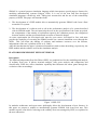
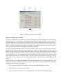
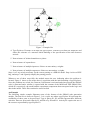
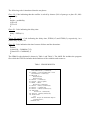
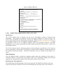
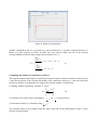
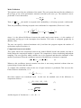
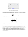
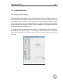
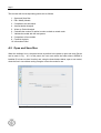
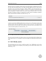
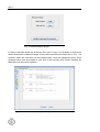
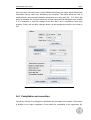
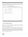
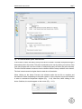
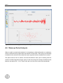
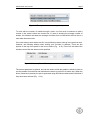
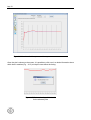
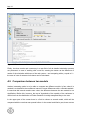
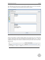
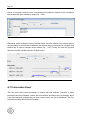
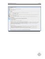
A performance analysis tool of discrete-event systems
Albert Peñarroya, Francesc Casado, Jan Rosell
IOC Divisió de Robòtica
IOC-DT-P-2007-1
Gener 2007
A PERFORMANCE ANALYSIS TOOL OF DISCRETE-EVENT SYSTEMS
Albert Peñarroya, Francesc Casado and Jan Rosell
Institute of Industrial and Control Engineering
Technical University of Catalonia, Barcelona, Spain
E-mail: [email protected]
A PERFORMANCE ANALYSIS TOOL OF DISCRETE-EVENT SYSTEMS
Albert Peñarroya, Francesc Casado and Jan Rosell
Institute of Industrial and Control Engineering
Technical University of Catalonia, Barcelona, Spain
E-mail: [email protected]
KEYWORDS
Petri nets, SIMAN, Discrete-event simulation, Computer-aided tools.
ABSTRACT
The analysis of the logic correctness of the system and its performance evaluation are usually
carried out using, respectively, the Petri nets formalism and the discrete-event simulation. Several
tools exist for both. The Platform Independent Petri Net Editor (PIPE) is a free software tool
developed in Java for the modeling, simulation and qualitative analysis of Petri nets. It has been
designed with an open philosophy so that extensions can be easily incorporated. SIMAN is one of
the first discrete-event simulation languages developed. It has extensively proven its power. This
paper first presents a module for the PIPE software that allows the automatic generation of SIMAN
code from a Petri net. Then, a tool is proposed to aid the performance analysis of manufacturing
systems from its SIMAN model. These tools are designed as a support for students in the
understanding of the simulation methodology.
INTRODUCTION
The two main objectives when analyzing a manufacturing system are the evaluation of the logical
correctness (i.e. the qualitative analysis) and the evaluation of its performance (i.e. quantitative
analysis). Petri nets formalism and discrete-event simulation are used to carry out these objectives
and, therefore, both must be included in the engineering students’ curricula (Desel, 2000). Taking
into account this, the objective of this paper is to introduce an aid to help students in the
understanding of the use of simulation techniques as a methodology for the analysis of
manufacturing systems.
Petri nets are a formalism that allows the modelling of systems involving concurrency, resource
sharing, synchronization and conflict, and allows the validation of the correctness of the system by
analyzing the qualitative properties of the net modelling the system (Murata, 1989). There are
several software tools (see the Petri Nets World web www.informatik.uni-hamburg.de/
TGI/PetriNets/tools/) that allow the modeling, simulation and analysis of Petri nets.
The Platform Independent Petri Net Editor (PIPE, http://pipe2.sourceforge.net/), is a Java based,
open source, graphical tool for drawing and analyzing Petri nets developed at the Department of
Computing at Imperial College London (Figure 1). Some of its available modules include invariant
analysis, simulation, state space analysis and comparison and classification. New modules can be
developed and easily incorporated.
SIMAN is a general purpose simulation language which incorporates special purpose features for
modeling manufacturing systems (Pedgen, 1986). It is one of the best and first developed
simulation languages extensively used. Taking into account this and the use of the extensibility
property of PIPE, this paper will introduce both:
1. The development of a PIPE module able to automatically generate SIMAN code from a Petri
net model of a system.
2. The development of a software tool to aid in the performance analysis of a system described
with its SIMAN model. The tool must help the user in the specification of the warm-up period,
the computation of the number of replication required, the validation process, the comparison
between models, and the specification and execution of factorial designs.
As extra requirements the developed tools must be open source, developed in Java, and must
provide the capability of executing the SIMAN models on a remote simulation server through the
WEB. This will allow the sharing of software and hardware resources over the Internet,
independent of the user’s platform (Guru et al., 2000).
After this introduction the paper is structured around two main sections describing, respectively, the
PIPE module and the software tool for the simulation analysis.
PLATFORM INDEPENDENT PETRI NET EDITOR
Description
The Platform Independent Petri Net Editor (PIPE) is a graphical tool for the modelling and analysis
of ordinary Petri nets. It allows invariant analysis, state space analysis and comparison and
classification. PIPE also offers simulation capability that illustrates the token game through the
evolution of the net markings.
Figure 1 PIPE GUI
Its modular architecture and open source philosophy allows the development of new features. In
this paper we propose a module to automatically generate SIMAN code from Petri nets. This
module requires some kind of coloring to the ordinary Petri nets managed by PIPE, as explained in
the next subsection.
Figure 2 SIMAN Code Generation Module
SIMAN code generation module
In order to include this new module, the following changes have been introduced to the basic PIPE
functionality. First, the capacity to distinguish between different types of places: type-A places to
represent activities, type-B places to represent finite resources like machines or robots, type-C
places for control places, and type-D places to represent the system input or variable resources like
pallets or fixtures. Second, the capacity to introduce code into the net places in order to specify
some parameters and values needed when translating to SIMAN.
In order to generate SIMAN code from a Petri net first it is necessary to specify the type of places
and the initial marking. Then the code associated to each place must be introduced. For type-A
places it is necessary to specify the delay time of the activity; for type-B places the time between
failures and the downtimes; for type-C places the group to which they pertain since type-C places
are grouped in sets; for type-D places the time between arrivals whenever they represent the system
input. Moreover if there is a conflict in type-A or type-D places it is necessary to specify how it is
to be solved (i.e. by chance or by the type of entity which is defined in the corresponding type-D
place).
Once the Petri net is defined, the SIMAN code generation module can be executed (Figure 2). The
module first makes a validation of the net in order to avoid future parsing problems. This validation
consists in the following verifications:
1. Type-A places: Existence of at least an input arc and initial marking set to zero.
2. Type-B places: Non-null initial marking.
3. Type-C places: Specification of a family group and non-null initial marking per group.
Figure 3 Example Net
4. Type-D places: Existence of at least one type-D place, existence of at least one output arc and
either the existence of a non-null initial marking or the specification of the time between
arrivals.
5. Non-existence of isolated transitions or places.
6. Non-existence of repeated arcs.
7. Non-existence of multiple input arcs if there are non-unitary weights.
8. Non-existence of multiple output arcs if there are non-unitary weights.
Steps 1 to 5 are strictly necessary for the correct parsing to a SIMAN model. Step 6 solves a PIPE
bug, and steps 7 and 8 greatly simplify the parsing process.
Whenever one of these steps fails, the module warns the user indicating where the problem is
located. Figure 2 shows a case where there is a problem with the initial marking of type-B places.
Once the problems are solved, the Generate Code button is activated and when pressed the SIMAN
code is generated and a window is opened with the contents of the MOD and EXP SIMAN files
which are, respectively, the model and the experiment components that correspond to the logic and
data in the model. These files can then be stored to disk.
An Example
The following simple example illustrates some of the features of the SIMAN code generation
module. The Petri net is shown in Figure 3. It is a cyclic net where type-D place P0 represents the
availability of three parts to be processed. Type-A places P1, P2 and P4 represent three different
activities. Parts are processed either by P1 and P4 or by P2 and P4. Activity P2 requires the use of
the resource represented by type-B place P3.
The following code is introduced into the net places:
Place P0: Code indicating that the conflict is solved by chance (20% of parts go to place P1; 80%
to place P2).
#
decide = probability
@T0=0.8
@T1=0.2
#
Place P1: Code indicating the delay time.
#
delay = EXPO(1.1)
#
Places P2 and P4: Code indicating the delay time, EXPO(0.5) and EXPO(2), respectively, in a
similar way as place P1.
Place P3: Code indication the time between failures and the downtime.
#
failures
@ timeON = GAMMA(7,15)
@ timeOFF = GAMMA(2,3)
#
The SIMAN code obtained is shown in Table 1 and Table 2. The MOD file includes the program
flow while the EXP file includes the definitions of the variables and resources.
Table 1. SIMAN MOD File
1$ CREATE, 3,HoursToBaseTime(0.0),Entity P0:
HoursToBaseTime(1),1: NEXT(2$);
2$ ASSIGN: Create P0.NumberOut = Create
P0.NumberOut + 1:NEXT(3$);
3$ BRANCH, 1:
With,0.8,4$,Yes:
With,0.2,5$,Yes;
4$ DELAY: 0: NEXT(6$);
5$ QUEUE, Seize T1.Queue;
7$ SEIZE, 2,Other:
Resource P3, 1:NEXT(8$);
6$ DELAY: EXPO(1.1):NEXT(9$);
9$ DELAY: 0: NEXT(10$);
8$ DELAY: EXPO(0.5):NEXT(11$);
11$ RELEASE:
Resource P3, 1:NEXT(10$);
10$ DELAY: EXPO(2):NEXT(12$);
12$ DUPLICATE:
1,3$;
ASSIGN: Dispose T4.NumberOut=Dispose
T4.NumberOut+1;
DISPOSE: Yes;
Table 2. SIMAN EXP File
PROJECT, "Unnamed Project", "Siman Code
Generation" ,,,No,Yes,Yes,Yes,No,No,No,No,No;
FAILURES:
Failure 0,Count(GAMMA(7,15),GAMMA(2,3));
RESOURCES:
Resource P3,Capacity(1),,,,, FAILURE(Failure
0,Ignore),;
REPLICATE, 10,,HoursToBaseTime(160),Yes,Yes,,,,
24,Hours,No,No,,,Yes;
VARIABLES:
Create P0.NumberOut, CLEAR(Statistics), CATEGORY
("Exclude"): Dispose T4.NumberOut,
CLEAR(Statistics),
CATEGORY("Exclude");
ENTITIES:
Entity P0;
QUEUES:
Seize T1.Queue,FIFO,,AUTOSTATS(Yes,,);
DSTATS:
Create P0.NumberOut, aCreate P0.NumberOut:
Dispose T4.NumberOut,aDispose T4.NumberOut;
CASA - COMPUTER AIDED SIMULATION ANALYSIS
Specification
The CASA software has as objective the aid in the performance analysis of discrete-event
simulations. The program has different features like model validation or factorial design. The
results of the simulations are obtained by executing the SIMAN models, or in some cases they can
be provided by data text files. The ARENA simulation software (www.arenasimulation. com) must
be available in order to use its SIMAN compiler, linker and simulation programs. The input
SIMAN files can be either generated by the PIPE module described in the previous section or by
the ARENA software.
The CASA software has the following options: model simulation, specification of the warm-up
period, computation of the number of replications required, model validation, comparison between
two models and factorial design. Theoretical expressions used are obtained from (Banks et al.
1996) .
Model simulation
Once the SIMAN model is loaded, the simulation utility allows the simulation of the model. A
command window is opened where the different calls to the compilation, linking and execution
programs are automatically performed. The output data is shown in text format.
Specifying the warm-up period
This option allows the determination of the warm-up period. The MOD file is shown to the user
where he specifies the variable to be used for determining the warm-up period. It can either be a
Figure 4 Warm-up Period Panel
variable computed at the exit of a block (e.g. parts produced) or a variable computed between to
blocks (e.g. time-in-queue or WIP). In either case, the software allows the use of the moving
average method to filter the data, using a chosen window size w:
⎧ w ~
⎪ ∑ Y i+s
⎪ s=− w
if i = w + 1,..., m − w
~
⎪ 2w + 1
Y i = ⎨ i −1 ~
⎪
Y i+s
⎪ s =∑
− ( i −1)
if i = 1,..., w
⎪
⎩ 2i − 1
(1)
Computing the number of replications required
This option computes the number of replications needed in order to obtain confidence intervals with
a specified precision. If the desired half-width of the confidence interval is ε, then the following
iterative procedure is programmed to compute the required number of replications:
1) Starting with R0 replications, estimate σ2 by S02:
S0 ⎤
⎡tα
, ( R −1)
⎢
⎥
2
R≥⎢
⎥
ε
⎢⎣
⎥⎦
2) Estimate a first value of R by substituting
tα
2
3) Increment R until (2) is satisfied (using t α
2
,( R −1)
,( R −1)
2
(2)
by z α in expression (2).
2
).
The program shows a text window with the final result and all the intermediate results of each
iterative step performed.
Model Validation
This option is an aid for the validation of the model. The real system data used for the validation is
the average of one of the performance measures selected by the user (μ0). The statistical t-test is
performed . First it determines:
y − μ0
t0 =
(3)
S/ n
Then, if t 0 < t α
the model is accepted with a probability α of having rejected a valid model.
2
,( n −1)
Then, the probability of having accepted a non-valid model is computed as (Ferris et al. 1946):
r
β =e
⎛1 2 ⎞
⎜ nλ ⎟
⎤
t ε2
1
⎝2
⎠ ⎡
(4)
I ⎢(r + 1 / 2 ), (n − 1);
∑
2 ⎥
r!
2
n −1 + tε ⎦
r =0
⎣
1
− nλ2 ∞
2
where λ is the allowed difference between the model and system means, n is the number of
replications and I(p,q;x) is the incomplete beta function. This value is computed graphically in
(Banks, 1996).
The user can specify a desired maximum risk β and then the program outputs the number of
replications required to achieve it.
Comparison between two models
This option allows the comparison between the loaded SIMAN model and another one that is
loaded when the comparison module is opened. The comparison is done considering independent
sampling. The user specifies which variables are to be compared and then the simulation of the
models is performed. Then the confidence interval of the difference of means is computed:
( (Y1 − Y2 ) ± tα ·s.e. (Y1 − Y2 ) )
2
(5)
,ν
Whenever this confidence interval contains zero there is not strong statistical evidence that one
system design is better than the other.
To compute this confidence interval, the test of equal variances is performed. This test uses the
Fisher-Snedecor distribution, i.e. if :
F=
S 22
< Fα , R1 −1, R2 −1
S12
(6)
then both variances are considered equal. In this case the standard error of the difference is
computed as follows:
SP
(
R1 − 1)·S12 + (R2 − 1)·S 22
=
s.e. = S P ·
R1 + R2 − 2
1
1
+
R1 R2
And the degrees of freedom are: ν = R1 + R2 − 2 .
(7)
(8)
Figure 6 Detail of the Factorial Results
Otherwise, when variances are considered unequal, standard error of the difference is computed as
follows:
S12 S22
+
R1 R2
(9)
⎤
⎡
2
⎥
⎢
2
2
⎛ S1 S 2 ⎞
⎥
⎢
⎜⎜
⎟
+
⎟
⎥
⎢
R
R
2 ⎠
⎝ 1
ν =⎢
⎥
2
2
2
⎛ S 22 ⎞ ⎥
⎢ ⎛⎜ S1 ⎞⎟
⎜ R ⎟ ⎥
⎢ ⎝ R1 ⎠
2⎠
+⎝
⎢
(R2 − 1) ⎥⎥
⎢ (R1 − 1)
(10)
s.e. =
and the degrees of freedom are:
As in other program options, all the computations are shown to the user in a text window.
Factorial design
The last option of the program allows the performance of a factorial design using up to six factors.
Each factor is assigned two values. The user selects the number of factors to consider and
introduces two values to be considered for each of them. The program automatically computes all
the possible combinations (design points) and executes the corresponding replicates of each one.
This option graphically outputs the confidence intervals of each of the principal effects of the
chosen factors (Figure 6). When the confidence interval does not include zero then the factor is
considered significant.
CONCLUSIONS
The availability of software tools for the understanding of the simulation methodology in the
analysis of manufacturing systems is a key aspect for engineering studies. This paper has proposed
two tools that cover both Petri nets and discrete-event simulation.
First, a module that automatically generates SIMAN code from Petri nets has been incorporated to
the Platform Independent Petri Net Editor (PIPE), an open source graphical tool for drawing and
analyzing Petri nets. Although PIPE allows the simulation of Petri nets, the translation to SIMAN
allows a better simulation of manufacturing systems since the new incorporated module permits,
among other features, the introduction of different time distributions or the definition of failures.
Moreover, the obtained SIMAN code facilitates the use of the second tool for the performance
analysis of the system.
The second tool introduced in this paper is the software CASA (Computer Aided Simulation
Analysis). It has been developed as an aid in the performance analysis of manufacturing systems
modeled using SIMAN. It has several features not encountered in other simulation packages, like
the capability of performing factorial designs or model validation.
Both tools are currently being used in undergraduate courses at the Industrial Engineering School of
Barcelona (Technical University of Catalonia). They are available at lafarga.cpl.upc.edu/.
REFERENCES
Banks, J., Carson J. and B. Nelson, 1996. Discrete-Event System Simulation. Prentice-Hall, Upper
Saddle River, NJ, USA.
Desel, J. 2000. “Teaching System Modelling, Simulation and Validation”, in Proceedings of the
2000 Winter Simulation Conference, pp. 1669-1675.
Ferris, C.L., Grubbs, F. E. and C. L. Weaver. 1946. “Operating Characteristics for the Common
Statistical Tests of Significance,” Annals of Mathematical Statistics, June 1946. The Institute of
Mathematicals Statistics
Guru, A., P. Savory and R. Williams. 2000. “A web-based interface for storing and Executing
Simulation Models”, in Proceedings of the 2000 Winter Simulation Conference, pp. 1810-1814.
Murata, T. 1989. "Petri Nets: Properties, Analysis and Applications," Proc. IEEE, vol. 77, No. 4
(Apr.), pages. 541-580.
Pedgen, C. D. 1986. “Introduction to SIMAN”, in Proceedings of the 1986 Winter Simulation
Conference, pp. 95-103.
APPENDIX:
CASA USER’S MANUAL
Page 1
Software CASA. User's manual.
A. CASA Manual
A.1 General Procedure
This software has been created in order to help the user to make a quantitative analysis of
the numeric results obtained after a discreet event simulation. Among the options it offers, we
could talk about warm-up period or auto-correlation, two-model comparison, factorial analysis
or determination of the number of replications needed. That’s why studying this parameters
can be automated and simplified. However, not all the variables can be analyzed because of
the characteristics of the simulation code.
The Graphic Interface is divided into panels, which can be selected clicking on the respective
tab on the left, as can be seen in Fig. A.1. Each panel is independent and can carry out the
chosen functionality, except panels one and two, which are meant to open and modify the
code files.
Fig. A.1 Tab-Based Structure
Page 2
The ten tabs with its corresponding panels are as follows:
1. Open and Save files
2. Edit / Modify Models
3. Compilation and simulation
4. Autocorrelation Analysis
5. Warm-up Period Analysis
6. Calculate the number of replica in order to obtain a certain result
7. Validate the model with the real system
8. Comparison of two models
9. Factorial Analysis
10. Information Panel
A.2 Open and Save files
When the software is run, the panel shown by default is the panel to open and save files as
can be seen in Fig. A.2. In this panel, the user must select the folder where ARENA is
installed (if he has not done it before) and, using the three buttons below, open a new model,
close the one in use without saving changes or save the model in use.
Fig. A.2 Panel to open and save files
Software CASA. User's manual.
Page 3
Although some of the software’s options can be used with text files containing numeric data,
the most useful and practical way to use CASA is through SIMAN code files. These files are
simulated using the Rockwell Automation software ARENA (www.arenasimulation.com),
which has an educational version available. To do this, it is necessary to specify the folder
where this software is installed, which can be done using the Browse button in the Arena
Path field. The folder is stored in an internal file, so that it won’t be necessary to specify it
again. Once the folder is selected, it is shown as in Fig. A.3.
Fig. A.3 Arena folder selected
In order to work with a SIMAN coded model, it must be in use. This action must be done
using the button Open and selecting the model .mod file in the drive. The experiment file
must be stored in the same folder and must have the same file name for the software to find
it. Once a model is opened, it is shown as in Fig. A.4.
Fig. A.4 Open, close and save file buttons. A model is in use.
If the user closes the model, the software returns to its previous state and the changes done
to the model are lost. If it is necessary to store the changes, the third button (Save) must be
used.
A.3 Edit / Modify models
This panel allows the user to edit or modify the model in use. Modifications can be done
manually or assisted by the computer just by clicking on the chosen button shown in the
monitor (Fig. A.5).
Page 4
Fig. A.5 Model Edition options
In order to manually modify any of the two files (.mod o .exp), it is necessary to click on the
chosen Edit button, in Manual Change. In both cases a window such as the one in Fig. A.6
is shown, where the code lines can be modified freely. Once the changes are done, Store
Changes button must be pressed to save them in the currently open model. Pressing Go
Back returns to the previous window.
Fig. A.6 .mod and .exp manually modifiing window
Software CASA. User's manual.
Page 5
If the user does not know how to modify SIMAN code directly, the option Modify Experiment
Parameters can be used to be assisted by the computer. This option allows the user to
modify failures, resources and replication parameters in an easy way (Fig. A.7). When this
option is activated, the computer shows the current experiment file information and modifies
it. It is necessary to save the changes every time that a line is modified to save them
properly. Finally, with the store changes button, all the changes are stored in the model in
use.
Fig. A.7 EXP file parameters modification window
A.4 Compilation and execution
This panel’s function is to simplify the compilation and simulation of the models. This process
is divided in four steps: compilation of the model file, compilation of the experiment file,
Page 6
linkage of both files and simulation. That is why this window has four buttons (Fig. A.8), one
per each step. Under the buttons, there is a window where the results of each step are
shown for the user to know if there is any problem.
Fig. A.8 Compilation and Simulation panel
A.5 Autocorrelation analysis
This panel is used to study the independence and randomness of the numeric values
obtained with the simulation of the model. The method consists in drawing the
autocorrelation graph and dispersion diagram.
When the user accesses this panel (Fig. A.9) two sections can be observed. There is the
option of using a text file at the top. The other area is needed to work with the model. If the
user wants to introduce the data with a text file, it must contain two columns separated by a
tabulator key. The first column must contain the timing and the second column the data to
analyse. Information about various replications must be added without any kind of extra
information, just repeating the timing column.
Page 7
Software CASA. User's manual.
Fig. A.9 Autocorrelation panel. Data selection
If the model is used, the data to study must be the number of entities that pass through a
determined point in the model. This point is selected by the user by clicking on one line of the
code (the program will count the number of entities that pass just before the point selected).
The time interval between measures must be defined with the camp available at the bottom.
The time interval cannot be higher than the total time of simulation.
When clicking on the button Proceed, the software reads the text file or compiles and
simulates the model, depending on the option chosen. In the next panel, lag must be defined
in order to calculate the dispersion diagram (Fig. A.10). After that, when clicking on the
button Graficate, the results appear on the screen (Fig. A.11).
Fig. A.10 Autocorrelation options
Page 8
Fig. A.11 Autocorrelation graph and dispersion diagram with chosen lag
A.6 Warm-up Period Analysis
When a model is created and simulated, it is interesting to obtain information in a stationary
mode, so that the warm-up period does not interfere in the results. That is why it is interesting
to determine the moment in time where the warm-up period can be considered to be ended.
This panel works as the one before, with the little difference that, apart of working with the
number of entities that pass through a point, it does also accept the average of entities stored
between two points.(Fig. A.12). If that is the case, two lines of the code must be selected.
Software CASA. User's manual.
Page 9
Fig. A.12 Two options in the warm-up period panel
To work with the number of entities through a point, one line must be selected to add a
counter in the model, before the chosen line. In case of studying the average number of
entities, the software calculates the average of entities from a mark before the first line to a
mark after the second one.
If the user wants to work with a text file, it must follow the same rules as in the previous case.
However, the following window when clicking over Proceed, is different. There are two
options on the top of the panel for the user to define (Fig. A.13). First of all, the wide of the
window used to filter the data must be specified.
Fig. A.13 Warm-up Period Panel options
The second parameter is optional, and can be used to divide the graphic in blocks in order to
see the median of each block and determine the warm-up period in an easier way. When the
button Generate is pressed, the plot is generated using the Welch method and the divisions if
they have been selected (Fig. A.14).
Page 10
Fig. A.14 Number of entities processed in a system
Once the plot is shown on the screen, it is possible to click over it to obtain information about
which time it matches (Fig. A.15) to help the user define the timing.
Fig. A.15 Window showing which time is
for the selected point
Software CASA. User's manual.
Page 11
A.7 Calculate the number of replica
The study that is done in this window consists in determining which is the number of replica
needed in order to have the confidence interval of one of the results of the simulation equal
to a selected 2·ε wide.
Regarding the graphic aspect and user interaction, when beginning this analysis a panel
similar to the previous is shown, but with some differences. The part designed to choose the
text file is identical, but in the part that uses the current SIMAN model a list appears with all
the variables about which it is possible to obtain information through simulation. (Fig. A.16).
Fig. A.16 Window to calculate the number of replica
Afterwards, when the Proceed button is clicked, a new screen is shown, where the user must
fill in two fields: which are the confidence desired for the statistic and the wide of the
confidence interval (Fig. A.17).
Page 12
Fig. A.17 Parameters needed to calculate the number of replica
Then, when clicking the Calculate button, the software reads the datum and carries out the
iterative calculations needed to determine the number of replica. The current and the desired
intervals, as well as the number of replica that are necessary or sufficient to achieve this
interval, are shown. Besides the final results, the software shows on the screen all the
iterative calculation so that the user can have the information of the process in detail (Fig.
A.18).
Fig. A.18 Result screen of the calculation of number of replica
Software CASA. User's manual.
Page 13
Finally, we must consider that when we introduce the datum as a text file, it should have a
specific layout. In fact, it should be introduced, as the form of a column, the medium value
that the variable has taken in each of the replica simulated.
A.8 Validate the model with the real system
The aim of the validation of a model panel consists in the verification of the kindness of the
results of the simulation through the comparison with the mean of the real system. Three
results are found:
ƒ acceptance or not of the model as valid
ƒ risk of accepting a non-valid model
ƒ number of necessary replica to respect a certain limit risk
The panel’s graphic structure is, in the beginning, similar to the former point. Thus, the user
can choose between using a text file or an opened model, of which he should select a
variable to be studied. The information in the text file must be presented in column form, in
order to have a correct datum interpretation.
In the second screen the user has got four fields to fill in before carrying out the calculations
(Fig. A.19). In the upper part, it is necessary to determine the value of the statistic for the
calculation of the interval (Ci% section) and which is the mean of the real system (Real
system mean). Moreover, it is necessary to fill in the field of the β desired value (maximum
risk of accepting a non-valid model which is allowed) and the λ value (maximum normalized
difference between the model mean and that of the real system)
Fig. A.19 Parameters to be established for the model validation.
Then, when clicking on the Calculate button the calculations with those values are realized
and the final results, as well as the calculation process, are shown on screen (Fig. A.20).
Furthermore, general information of the datum with the mean, the variance and the number
of replica, is shown, in order to help the user to adjust the real parameters.
Page 14
Fig. A.20 Result screen of the model validation.
Finally, the three results and a summary in a text field of all de detailed calculation process
are presented. In case of working with a text file, entering the datum as the difference of
results of the simulation with those of the real system – and comparing with a µ equal to 0 –
the case of a set of entrance /exit datum can be calculated.
A.9 Comparison between two models
Another interesting option is to be able to compare two different models. In fact, what it is
needed is to determine the confidence interval of mean differences with a t-Student statistic.
In case that this interval contains zero value, the difference between the two models is not
significative. Before this, however, the test of hypothesis of the equality of the variances is
carried out from the distribution of Fisher-Snedecor in totally transparent way to the user.
In the upper part of the screen there is a field to choose a second model, which will be
compared with the one that was opened before. In the central and inferior part, there are two
Software CASA. User's manual.
Page 15
lists. With these two lists the user can select which variable will be used in the comparation
(Fig. A.21). Clicking on the Proceed button the next screen is shown.
Fig. A.21 Screen for the comparison between two models
If there is any problem, a warning message appears on the screen and, if not, a new screen
is shown. In this screen the user must select the two parameters shown in Fig. A.22: the
confidence percentage for the interval to calculate and the queue area value for the FisherSnedecor test.
Fig. A.22 Parameters to determine for the two models comparison
Page 16
When clicking the Calculate button the software realizes all the required calculations and
draws on the screen (Fig. A.23) the found interval as well as other datum of interest related
to the calculations.
Fig. A.23 Result screen of comparison between two models
A.10 Factorial Analysis
In most of simulation studies it is necessary to compare configuration alternatives or different
scenarios in order to be able to choose the one with the best results, while taking the
disposable resources into account. The factorial design is used to study this type of
comparison. This software permits to carry out a factorial study at two levels through two and
six factors. In the upper part of the factorial analysis screen there is a slider bar (Fig. A.24)
used to select the number of effects.
Software CASA. User's manual.
Page 17
Fig. A.24 Selection of the number of effects
Then, clicking the Continue button, the effects can be specified. To specify them, it is
necessary to change the lines of the model or experiment files in a space in the screen’s
inferior part. The original line corresponds to the “-“ level, whereas the modified one
corresponds to the “+” level (Fig. A.25). Thus, a same line can not be twice modified, since
the program interprets the change like a single line. To choose among the .mod and .exp
files there are two radio buttons that generate a new list of the former type.
Fig. A.25 Specification of + levels for the factorial design.
When all effects have already been introduced, the software carries out all the combinatory
of effects and levels automatically, does the pertinent simulations and goes to the following
Page 18
screen. In this new screen the user must specify the confidence desired for the confidence
interval and with which variable to study (Fig. A.26).
Fig. A.26 Parameters for the calculation of the factorial design effects
Afterwards, when clicking the Select Variable button, the main effects of the several factors
are calculated, as well as their confidence interval and they are presented in a graphic and
intuitive way in order to compare all the effects (Fig. A.27). Finally, the user can go back
and select another variable with the Go Back button.
Fig. A.27 Result screen of the factorial analyisis
A.11 Informative Panel
This last panel offers extra information in relation with this software. Precisely, it offers
information about the software version, about the authors and about the Colt package, which
is the free statistical package that has been used to carry out some calculations. The Fig.
A.28 shows exactly which is this information.
Software CASA. User's manual.
Fig. A.28 Information Panel
Page 19