Download Theorem Proving Support - Developers Manual

Grant Agreement: 287829
Comprehensive Modelling for Advanced Systems of Systems
Theorem Proving Support - Developers Manual
Technical Note Number: D33.2b
Version: 1.0
Date: September 2013
Public Document
http://www.compass-research.eu
D33.2b - Theorem Proving Support - Dev. Man. (Public)
Contributors:
Simon Foster, UY
Richard Payne, NCL
Editors:
Simon Foster, UY
Richard Payne, NCL
Reviewers:
Juliano Iyoda, UFPE
Jan Peleska, UB
Luís D. Couto, AU
2
D33.2b - Theorem Proving Support - Dev. Man. (Public)
Document History
Ver
0.01
Date
24-05-2013
Author
Richard Payne
0.02
06-06-2013
Richard Payne
0.03
18-06-2013
Richard Payne
0.04
02-07-2013
Richard Payne
0.05
08-07-2013
Simon Foster
0.06
16-07-2013
Richard Payne
0.07
0.08
23-08-2013
30-08-2013
Simon Foster
Richard Payne
0.09
03-09-2013
Richard Payne
0.10
09-09-2013
Simon Foster
0.11
09-09-2013
Richard Payne
0.12
18-09-2013
Richard Payne/Simon Foster
0.13
23-09-2013
Richard Payne/Simon Foster
0.14
23-09-2013
Richard Payne/Simon Foster
1.0
23-09-2013
Richard Payne/Simon Foster
3
Description
Initial document version
Initial summary and
introduction
Split into two documents
Adding doc overview
and labels etc
Material added for
development of Isabelle/UTP
and
tutorials
Initial draft of document for first milestone
Added sections 2,3,4
Finished introduction
and initial conclusions
Finished
material
added for plugin and
conclusions
Updated introduction
and conclusion
Minor corrections for
final draft
LDC review comments
addressed
JI review comments
addressed
JP review comments
addressed
Final revisions for EC
D33.2b - Theorem Proving Support - Dev. Man. (Public)
Summary
Work Package 33 delivers a collection of static analysis tool support for reasoning in CML. This deliverable forms the documentation for Task 3.3.2 –
theorem proving. Deliverable D33.2 forms two parts: executable code and
documentation.
The documentation is provided in two documents. This document, D33.2b,
is the second part; the technical details of the theorem proving support,
which provides details on background of theorem proving, the development
of theorem proving support for CML, the theories for UTP and of CML
itself and the theorem prover COMPASS plugin. The document finishes
with details of examples of two CML models and their equivalent Isabelle
theory.
This part of the deliverable highlights the main achievements of Task 3.3.2:
• The Isabelle/UTP theories provides the basis for the mechanisation
of CML. The theories are substantial pieces of work and, with the
developed automated proof tactics, are usable for non-experts.
• Building on the aforementioned UTP theories, the Isabelle/CML theories provide the ability to reason over a substantial subset of the CML
language. Automated proof tactics and a simple proof strategy for
solving finite set conjectures have been developed.
• The COMPASS theorem prover plugin provides a translation from a
CML model defined in the COMPASS tool platform to an Isabelle theory for model-specific proof. The plugin, therefore, acts as a component
of the mechanisation of the CML denotational semantics.
The first part of the Deliverable D33.2, D33.2a - User Manual, provides
details on obtaining and installing the theorem proving support for CML, and
also how to use the theorem prover tool within the COMPASS platform.
4
D33.2b - Theorem Proving Support - Dev. Man. (Public)
Contents
1 Introduction
7
1.1 Overview of theorem proving with Isabelle . . . . . . . . . . . 7
1.2 Summary of deliverable . . . . . . . . . . . . . . . . . . . . . . 10
2 Mechanising the UTP and CML
2.1 Deep or Shallow? . . . . . . . . . . . . . . . .
2.2 Isabelle/UTP overview . . . . . . . . . . . . .
2.3 A Parametric Predicate Model . . . . . . . . .
2.4 Value sorts . . . . . . . . . . . . . . . . . . . .
2.5 Expressions . . . . . . . . . . . . . . . . . . .
2.6 Relations and Imperative Programming . . . .
2.7 Complete Lattices, Fixed-points and Iteration
2.8 UTP Parser . . . . . . . . . . . . . . . . . . .
2.9 Automated Proof . . . . . . . . . . . . . . . .
2.10 Supporting theorems and attributes . . . . . .
2.11 Shallow Expressions . . . . . . . . . . . . . . .
2.12 Channels and Events . . . . . . . . . . . . . .
.
.
.
.
.
.
.
.
.
.
.
.
.
.
.
.
.
.
.
.
.
.
.
.
.
.
.
.
.
.
.
.
.
.
.
.
.
.
.
.
.
.
.
.
.
.
.
.
.
.
.
.
.
.
.
.
.
.
.
.
.
.
.
.
.
.
.
.
.
.
.
.
.
.
.
.
.
.
.
.
.
.
.
.
.
.
.
.
.
.
.
.
.
.
.
.
.
.
.
.
.
.
.
.
.
.
.
.
11
11
12
13
17
18
19
20
23
25
30
32
35
3 Mechanising a UTP theory
3.1 Design Alphabet . . . . . . . .
3.2 Design Signature . . . . . . . .
3.3 Design Healthiness Conditions .
3.4 The Theory of Designs . . . . .
3.5 The Theory of Normal Designs
3.6 The Theory of Feasible Designs
3.7 Conclusion . . . . . . . . . . . .
.
.
.
.
.
.
.
.
.
.
.
.
.
.
.
.
.
.
.
.
.
.
.
.
.
.
.
.
.
.
.
.
.
.
.
.
.
.
.
.
.
.
.
.
.
.
.
.
.
.
.
.
.
.
.
.
.
.
.
.
.
.
.
.
.
.
.
.
.
.
.
.
.
.
.
.
.
.
.
.
.
.
.
.
.
.
.
.
.
.
.
.
.
.
.
.
.
.
.
.
.
.
.
.
.
.
.
.
.
.
.
.
.
.
.
.
.
.
.
38
38
39
49
63
66
66
66
4 A Theory of CML Processes
4.1 CML Value Domain . . . . . . . .
4.2 CML Predicates and Expressions
4.3 CML Actions and Processes . . .
4.4 Undefinedness . . . . . . . . . . .
4.5 CML Proof Goals . . . . . . . . .
.
.
.
.
.
.
.
.
.
.
.
.
.
.
.
.
.
.
.
.
.
.
.
.
.
.
.
.
.
.
.
.
.
.
.
.
.
.
.
.
.
.
.
.
.
.
.
.
.
.
.
.
.
.
.
.
.
.
.
.
.
.
.
.
.
.
.
.
.
.
.
.
.
.
.
.
.
.
.
.
67
67
72
75
77
80
.
.
.
.
82
82
84
86
86
5 COMPASS tool theorem prover plugin
5.1 Architecture . . . . . . . . . . . . . . . .
5.2 Visitor behaviour . . . . . . . . . . . . .
5.3 Integration with the COMPASS platform
5.4 Translation examples . . . . . . . . . . .
5
.
.
.
.
.
.
.
.
.
.
.
.
.
.
.
.
.
.
.
.
.
.
.
.
.
.
.
.
.
.
.
.
.
.
.
.
.
.
.
.
.
.
.
.
D33.2b - Theorem Proving Support - Dev. Man. (Public)
5.5
Summary . . . . . . . . . . . . . . . . . . . . . . . . . . . . . 91
6 Examples
93
6.1 Bit Register . . . . . . . . . . . . . . . . . . . . . . . . . . . . 93
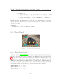
6.2 Dwarf Signal . . . . . . . . . . . . . . . . . . . . . . . . . . . . 96
7 Conclusion
106
7.1 Main achievements . . . . . . . . . . . . . . . . . . . . . . . . 106
7.2 Further work . . . . . . . . . . . . . . . . . . . . . . . . . . . 108
Appendices
113
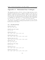
A Mechanised Law Catalogue
A.1 Predicate Laws . . . . . . . . .
A.2 Relational Laws . . . . . . . . .
A.3 Basic Refinement Laws . . . . .
A.4 Lattice Laws . . . . . . . . . . .
A.5 Fixed Point and Recursion Laws
A.6 Iteration Laws . . . . . . . . . .
A.7 Hoare Logic Laws . . . . . . . .
A.8 Weakest Precondition Laws . .
A.9 Design Laws . . . . . . . . . . .
6
.
.
.
.
.
.
.
.
.
.
.
.
.
.
.
.
.
.
.
.
.
.
.
.
.
.
.
.
.
.
.
.
.
.
.
.
.
.
.
.
.
.
.
.
.
.
.
.
.
.
.
.
.
.
.
.
.
.
.
.
.
.
.
.
.
.
.
.
.
.
.
.
.
.
.
.
.
.
.
.
.
.
.
.
.
.
.
.
.
.
.
.
.
.
.
.
.
.
.
.
.
.
.
.
.
.
.
.
.
.
.
.
.
.
.
.
.
.
.
.
.
.
.
.
.
.
.
.
.
.
.
.
.
.
.
.
.
.
.
.
.
.
.
.
114
. 114
. 117
. 126
. 127
. 128
. 128
. 129
. 130
. 131
D33.2b - Theorem Proving Support - Dev. Man. (Public)
1
Introduction
Formal verification techniques aim to prove the correctness of a system model
with respect to a specification, allowing users to confirm or refute, with a high
level of confidence, properties of a model. There are two main methods of
formal verification - model checking and theorem proving. Model checking
support is provided in Task T3.3.1, and theorem proving in Task T3.3.2.
This deliverable details the theorem proving support of Task T3.3.2.
Theorem proving entails the symbolic justification of an assertion using a
collection of axioms, rules and previously asserted facts. The collection is
termed a theory, which may describe different logics (such as first-order predicate logic), complex datatypes (such as lists and mappings) and functional
languages (including HOL). Given a theory, arbitrary theorems and lemmas
may be proven.
Theorem proving may be provided manually through hand written proofs
or with a degree of machine-support. Hand-written proofs, such as those
presented in the CML definition [BCC+ 13], tend to result in proofs which are
easier for a human user to understand. However, human errors are more likely
in large unwieldy proofs. Automated theorem proving, and proof assistants
are a rapidly advancing area of academic research.
Several tools, providing a range of automated proof support are available.
For example, Isabelle1 is a generic proof assistant in that any calculus may
be used (higher order logic (HOL) is most commonly used), PVS2 is a verification system, combining a specification language with a theorem prover,
HOL43 is an interactive proof assistant for higher order logic, and Rodin4 is a
platform for the Event B formal method which supports automated theorem
proving. Such automated theorem provers would require either a shallow or
a deep embedding of a CML model in which proofs are to be carried out and
the underlying CML language.
1.1
Overview of theorem proving with Isabelle
In the COMPASS project, we use the Isabelle proof assistant. Isabelle, under
development for the last 25 years, is a generic system for implementing logical
1
http://isabelle.in.tum.de
http://pvs.cdl.sri.com
3
http://hol.sourceforge.net
4
http://www.event-b.org
2
7
D33.2b - Theorem Proving Support - Dev. Man. (Public)
formalisms – the most widely used of which is HOL (Higher-Order Logic),
providing functional programming and logic.
Isabelle is a generic proof assistant – providing decidable proof checking over
assertions in a given logic. Isabelle proofs are classed as LCF-style – that is
proofs are correct by construction based on previously proven theorems which
in turn are proven in terms of a small core set of axioms. Isabelle/HOL builds
upon a large library of theories (including sets, lists, lattices and more), which
are built through inheritance.
Proofs in Isabelle are defined as scripts which manipulate a proof state (the
assertions and previously proven rules) in an effort to discharge a particular
conjecture. Scripts update the proof-state, splitting and simplifying goals.
Proven theorems may subsequently be used in future proofs.
Isabelle has several tools to automatically identify counterexamples and automatically determine proof scripts. These tools include the counterexample
generators nitpick [BBN11] and quickcheck, the simplifying term rewriter
simp, the automated deduction tactic blast [Pau99], auto which combines
simp and blast, and finally sledgehammer [BBN11] which dispatches theorems to several remote automated theorem provers. Given a proposed solution, Isabelle’s built-in proof reconstruction agent metis [Hur03] proves the
validity of the solution.
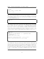
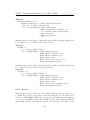
Isabelle proofs can be written in two ways. The first is the apply-style, where
the user issues a sequence of commands to variously divide and conquer a
proof, using a variety of the proof tactics mentioned above. Apply scripts are
powerful and make proof automation easier, however they are not readable
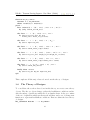
by humans. The second is the Isar proof language, where proofs can be
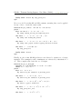
written in a more calculational way. For instance, there follows an Isabelle
proof of a form of Cantor’s theorem.
theorem Cantor:
fixes f :: "’a ⇒ ’a set"
shows "∃ S. S ∈
/ range f"
proof
let ?S = "{x. x ∈
/ f x}"
show "?S ∈
/ range f"
proof
assume "?S ∈ range f"
then obtain y where "?S = f y" ..
thus False
proof (rule equalityCE) — y in both sets or neither
assume "y ∈ f y"
8
D33.2b - Theorem Proving Support - Dev. Man. (Public)
assume
with ‘y
next
assume
assume
with ‘y
qed
qed
qed
"y ∈ ?S" then have "y ∈
/ f y" ..
∈ f y‘ show ?thesis by contradiction
"y ∈
/ ?S"
"y ∈
/ f y" then have "y ∈ ?S" ..
∈
/ ?S‘ show ?thesis by contradiction
This proofs shows that there can be no bijection between an infinite set and
its powerset. This is proved by showing there is no surjection from a set to
its powerset. There is always an element which must be left out of the range:
∃S.S ∈
/ rangeF . We prove this by contradiction, assuming that such a value
exists and showing that False necessarily follows.
The Isabelle tool is extendable to support additional logics. In Task T3.3.2,
therefore, we develop theories to support theorem proving in CML. The theories, described in more detail later in this document, provide a mechanisation
of the CML semantics defined in [BCC+ 13]. Ultimately this work enables us
to prove the soundness of the semantics of CML and prove theorems about
CML specifications. So to enhance usability of this work, the theory has
been developed to include a generic parser for UTP expressions, automated
proof tactics and a substantial library of proven algebraic laws.
The task has also developed an integration with the COMPASS tool platform [CML+ 13] as a theorem proving plugin. Part A of this deliverable [FP13]
constitutes the user manual of this plugin, and in this document, Part B, we
present the technical description of the tool. The aim of the plugin is to
enable a non-expert to prove theorems about arbitrary CML specifications,
generating a model-specific CML theory with which Isabelle proofs may be
constructed.
It is beyond the scope of this document to provide detailed descriptions of
the Isabelle tool, or to provide a tutorial on it’s use. We therefore recommend that interested parties should read this deliverable in conjunction with
tutorials on Isabelle and proving in the Isabelle tool, available on the Isabelle website5 . A comprehensive account of the different syntactic elements
of Isabelle can be found in the Isabelle Reference Manual (also available on
the Isabelle website), which will aid in understanding the various Isabelle
definitions in this deliverable.
5
http://isabelle.in.tum.de/documentation.html
9
D33.2b - Theorem Proving Support - Dev. Man. (Public)
1.2
Summary of deliverable
The remainder of this document is structured as follows: in Section 2, we
describe the approach taken to develop theorem proving support for CML in
the Isabelle/UTP semantic framework, including a description of the theories
of UTP and CML. Section 3 describes the mechanisation of the UTP theory
of designs and Section 4 details the theory of CML. The theorem prover
plugin for the COMPASS tool platform is introduced in Section 5. Given the
technical description, in Section 6 we provide some example CML models
and describe the resultant theory models and how theorems may be proven
for the given model. Finally Section 7 provides conclusions on the technical
work carried out in the task and provides a discussion on the future work of
the task.
10
D33.2b - Theorem Proving Support - Dev. Man. (Public)
2
Mechanising the UTP and CML
Isabelle/UTP [FW13] is an implementation of Hoare and He’s Unifying Theories of Programming (UTP) [HJ98] in the Interactive Theorem Prover (ITP)
Isabelle/HOL [NWP02]. The UTP has been used to give a denotational and
operational semantics to CML in [BCC+ 13], and therefore if we are to prove
theorems about a CML specification, we need to mechanise the UTP. In this
Section we give a complete exposition of the development of Isabelle/UTP,
including the rationale for our design decisions and the wider implications
and applications for the library.
2.1
Deep or Shallow?
When mechanising any language or logic a key question to answer is whether
to make the embedding of the language deep or shallow, though this distinction is more of a spectrum than a straightforward dichotomy. Deep and
shallow embeddings essentially trade-off accuracy of encoding and ease of
proof. A deep embedding precisely mechanises the semantics of a language
and enables proofs about the soundness of the semantics of this language.
However, much more work is involved since the language must be described
from first principles.
In contrast a shallow embedding approximates the language constructs of
theory in terms of the implementation language. The major advantage of
this approach is that existing functions and proof tactics can be directly
used. The HOL logic for instance has a large library of mathematical and
programming language theories, as well as a number of well-developed proof
tactics, and it would be wasteful to not make use of these. There is a great
deal of similarity between VDM/CML and HOL, in as much as both are
essentially functional programming languages with the ability to write logical constraints over the programs. There are also key differences, such as
VDM being based on union types rather than algebraic data types, and these
challenges must be overcome in a shallow embedding. Nevertheless, these differences do not seem insurmountable, particularly when the prize is advanced
proof automation.
Nevertheless, there is a lot to be said for a deep embedding as well. If we
simply approximate the constructs of the language, how do we know what
the proof of a property mapped from CML into HOL really means? It’s all
very well to be able to discharge such proofs, but unless we can really say that
11
D33.2b - Theorem Proving Support - Dev. Man. (Public)
this has meaning in CML the stability of final system will be questionable.
Indeed one of the main purposes of the UTP is to give theories a denotational
semantics, such that we have a well-defined mathematical domain into which
all the operators of our language can be mapped, and the semantics of those
operators studied.
Since we observe the spectrum, we prefer an approach which attempts to
combine the best elements of both. Isabelle/UTP could be called a hybrid
embedding of the UTP. It is neither clearly a deep embedding nor a shallow
embedding but really exists in two layers, a deeper layer and shallower layer,
with a link between the two. We can, on the one hand, make use of existing
HOL types, functions and proofs, but we also have the ability to descend to
a deeper semantic level, using well known techniques from programming language semantics such as type erasure. We therefore often have twin concepts
in the language: for instance variables exist both in the deep and shallow levels. This then gives us the environment in which we can both: 1) mechanise
and prove soundness of the semantics of CML, and 2) prove theorems about
CML specifications produced by the COMPASS Proof Obligation Generator
(POG) by making use of HOL tactics.
Isabelle/UTP builds on and is inspired by two previous mechanisations of the
UTP: a shallow embedding of Circus in Isabelle called IsabelleCircus [FGW12]
which has been used to mechanise Circus refinement proofs, and a “deeper”
embedding in ProofPower-Z [OCW13] from which our predicate model is
in large part adapted. Our goal is to unify the advantages of these two
implementations.
2.2
Isabelle/UTP overview
Isabelle/UTP is a substantial mechanised theory library for Isabelle/HOL.
Different to a typical language mechanisation we do not begin with syntax,
that is we do not create a datatype which reflects the constructs available
in the UTP or CML. This is because the UTP is inherently extensible, and
new operators are given by definition – i.e. by defining them in terms of the
underlying UTP domain, as opposed to declaring their existence and then
later giving them a semantics. The UTP domain is provided by binding sets
which are described in Section 2.3. Binding sets are used to formalise first
predicates with which first-order logic formulae can be written and relations
which are used to formalise imperative programming operators and relational
specifications, such as Z-schemas. With this foundation the theories which
underlie CML are formalised.
12
D33.2b - Theorem Proving Support - Dev. Man. (Public)
A major aim of Isabelle/UTP is usability: we desire a library in which a
UTP theory can be mechanised by someone who is not an Isabelle expert
and doesn’t know the underlying encoding of UTP predicates. Usability is
provided in three main ways:
• Generic Parser for UTP expressions. This allows the theory engineer to write syntax in an intuitive way which hides the underlying
complexity of the UTP encoding, and also extend it with their own
new operators. Eventually we also extend this parser with CML expressions.
• Automated Proof Tactics which can solve a variety of conjectures
about UTP predicate and relations. These largely act as shims between
the UTP and existing Isabelle tactics.
• Algebraic Law Library. We have built a large library of proven
algebraic laws which can be used in conjunction with Isabelle’s sledgehammer tool to aid proof when the proof tactics fail. A catalogue of
these laws can be found in Appendix A.
Hence Isabelle/UTP can be used to extend the existing mechanised CML
theories with additional concepts, such as time, pointer theory, object orientation and mobility, whilst making use of all the theories developed so far.
This is important in the development of a language like CML, where the
requirements and semantics may need to evolve over time.
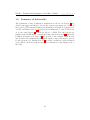
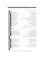
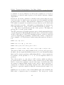
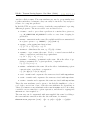
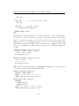
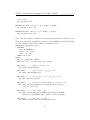
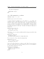
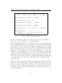
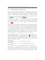
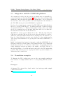
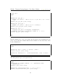
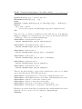
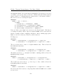
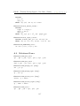
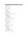
An overview of the Isabelle/UTP directory structure in Figure 1 gives some
idea of what has been mechanised so far. We now begin the main exposition
of Isabelle/UTP.
2.3
A Parametric Predicate Model
Predicates form the basis of the theory of CML, and therefore we mechanise
them first. In the UTP we do not start with syntax, but rather a semantic
domain in which all of the operators of our language can be given a denotation. A predicate is encoded as a set of variable bindings, specifically the
valuations which make the predicate true. For instance the predicate x > 7
would be represented by the set of bindings {x = 8, x = 9, x = 10 · · · }. A
binding is a function from variable names to values, var → val. The logic of
HOL is based on total functions and hence we also require that bindings are
total; variables irrelevant to the valuation of a predicate simply map to all
13
D33.2b - Theorem Proving Support - Dev. Man. (Public)
/
alpha.....................................Alphabetised Predicates
core
utp_binding.thy.............................Variable bindings
utp_expr.thy.................................Core expressions
utp_hoare.thy....................................Hoare Logic
utp_lattice.thy................................Lattice theory
utp_names.thy.................................Variable names
utp_pred.thy ............................ Core predicate model
utp_recursion.thy ....... Fixed points, Recursion and Iteration
utp_rel.thy..........................Core relational operators
utp_rename.thy......................Permuation and renaming
utp_sorts.thy.....................................Value sorts
utp_unrest.thy ......................... Unrestricted Variables
utp_value.thy ................................ UTP value class
utp_var.thy.........................................Variables
utp_wp.thy....................Weakest Precondition Semantics
models
utp_cml..................CML value model and function library
utp_vdm
laws
utp_pred_laws.thy ............................ Predicate Laws
utp_rel_laws.thy ...................... Relation Algebra Laws
utp_refine_laws.thy ........................ Refinement Laws
utp_rename_laws.thy..............Permuation/Renaming Laws
utp_subst_laws.thy.........................Substitution Laws
parser......................................UTP parser grammar
poly............................HOL-typed values and expressions
tactics
utp_expr_tac.thy ...................... Core Expression Tactic
utp_pred_tac.thy.............................Predicate Tactic
utp_rel_tac.thy.............................Relational Tactic
utp_subst_tac.thy.........................Substitution Tactic
theories
utp_csp.thy ................................... Theory of CSP
utp_definedness.thy ................. Theory of Undefinedness
utp_designs.thy............................Theory of Designs
utp_reactive.thy ................ Theory of Reactive Processes
types
utils
Figure 1: Isabelle/UTP directory structure (selection)
14
D33.2b - Theorem Proving Support - Dev. Man. (Public)
possible values (upward closure). So in x > 7 for instance variable y (and
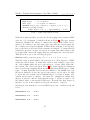
indeed z etc.) would also be present, but completely unconstrained.
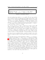
class DEFINED =
fixes Defined :: "’a ⇒ bool" ("D")
class VALUE = DEFINED +
fixes
utype_rel :: "’a ⇒ nat ⇒ bool" (infix ":u " 50)
assumes utype_nonempty: "∃ t v. v :u t ∧ D v"
Listing 1: The VALUE class
We also require that bindings are well-typed, which ensures that proofs about
predicates are simpler as they need not separately discharge soundness properties. Variables in Isabelle/UTP carry a name and type, and we require that
any binding must map each variable to a value of the correct type. Naturally we also need therefore to understand what kinds of values and types are
available. We could fix the kinds of types and values which are available, but
this seems against the spirit of the UTP which does not assume a particular
value domain. Indeed different formal languages may desire different notions
of values and typing. Therefore we make our predicate model parametric
over a user supplied value model, using parametric polymorphism. A value
model is a collection of HOL types, functions and properties which describe
the domain of values available. CML, for instance, consists of the standard
VDM types, such as int, seq of char and map nat to real, and these are all
described in the CML value model. We axiomatise value models using the
VALUE type class as shown in Listing Table 1. The user must supply four
things:
1. a value sort type α, representing possible value structures;
2. a typing sort type τ (must be countable);
3. a typing relation _ : _ :: α ⇒ τ ⇒ bool;
4. a definedness predicate D :: α ⇒ bool.
The requirement of a countable type sort derives from the fact that Isabelle
type-classes may carry only a single type-parameter. This limitation makes
type-inference decidable. For the VALUE class this type-parameter is the
sort of values α, and therefore we cannot also give τ its own type-parameter.
Instead we require that τ be injectable into nat, and its domain is described
by the typing relation. That is τ = {t | ∃v. v : t ∧ D(v)}: the set of types is
15
D33.2b - Theorem Proving Support - Dev. Man. (Public)
those for which there exists at least one defined value. We describe this type
as ’a UTYPE, and it is isomorphic to τ .
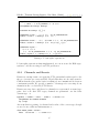
datatype SUBSCRIPT = Sub "nat" | NoSub
datatype NAME = MkName string nat SUBSCRIPT
type_synonym ’a VAR =
"NAME × ’a UTYPE × bool"
typedef ’a WF_BINDING =
"{b . ∀ v::’a VAR. b v B v}"
type_synonym ’a WF_PREDICATE =
"’a WF_BINDING set"
Listing 2: Isabelle/UTP basic types
With the value model defined, we can now describe the variable, binding and
predicate types, which are shown in Listing 2. A NAME consists of a string, a
nat denoting the number of dashes, and a SUBSCRIPT. A variable ’a VAR is a
name, together with a UTP type and auxiliary flag (to distinguish auxiliary
variables from program variables). A binding is described as the subset of
functions b :: α VAR ⇒ α such that each variable v maps to a compatible
value, denoted by b v B v. Finally, a predicate is described simply by a set
of bindings.
This encoding makes for a straightforward definition of most of the predicate
operators, since they map directly on the set functions. For instance, ∧,
∨, ¬, true and false are mapped onto ∪, ∩, − (set complement), UNIV
(the universe set) and {}. Therefore reasoning about these operators can
directly make use of the set theoretic laws formalised in HOL (we will say
more about this in Section 2.9). Implication is defined in the usual fashion:
(P ⇒ Q) , ¬P ∨ Q
Quantifiers are a little more tricky since we have invented our own notion
of variables. Nevertheless, since our underlying representation of bindings is
functions we can encode the quantifiers using function override. The function
override operator “f ⊕g on vs” is a ternary operator which overrides function
f :: α ⇒ β with function g :: α ⇒ β on the range of values given by
set vs :: α set. The existential quantifier can be defined thusly: (∃x.P ) ,
{b ⊕ b0 on {x}|b ∈ P }, that is we override the existentially quantified variable
16
D33.2b - Theorem Proving Support - Dev. Man. (Public)
with all possible bindings. Universal quantification can be defined in terms
of existential quantification in the usual way: (∀x.P ) , (¬∃x.¬P ).
Since we have formalised our own notion of variable, we also need to define
manipulation of these variables, in particular the α-conversion operator. We
have adopted the notion of a permuation from Nominal Logic [Pit01, Urb08]
for this. A permuation f :: α VAR ⇒ α VAR is a type-preserving bijection on
variables. Limiting permutations to bijections ensures nice algebraic properties such as f −1 ◦ f = id. The permutation of a predicate P by function f is
defined thusly: f • P , {b ◦ f −1 | b ∈ P }. The resultant bindings in P will
map the values of the renamed variables to those of the originals.
As well as α-conversion we also define a useful HOL predicate UNREST ::
(α VAR) set ⇒ α WF_PREDICATE ⇒ bool (sometimes abbreviated to ]), which
describes when a given set of variables is unrestricted by a predicate. That
is to say changing the value of one of these variables will not alter the truthvaluation of the predicate. Unrestriction is effectively a semantic encoding of
fresh variables, which can be used to encode predicate alphabets. Specifically
the restricted variables must appear in the alphabet of a predicate, whilst
the unrestricted ones appear optionally.
2.4
Value sorts
We have implemented a generic model of values and predicates, but as yet
we have said little about what kinds of values and types are available. UTP
theories often assume that particular types of values are constructible for use
in auxiliary variables. For instance the theory of designs assumes the presence
of boolean values for ok and ok 0 , and the theory of reactive processes assume
the presence of lists to represent traces in tr and tr0 . So in order for a value
domain to be usable in these contexts we need to axiomatise some notions
of values.
We could chose to constraint all models to contain a certain set of types, such
as booleans, integers, and lists. But the problem is where to stop. What
about sets? What about functions? Instead we opt for a more contractual
approach to value type constraints. The UTP theory in question requires
that any model which wishes to use designs must implement certain things,
and in return guarantees that its theorems hold in this context.
We implement this idea through value sorts. A value sort is a type-class which
subclasses the main VALUE class, adding addition constants and theorems.
17
D33.2b - Theorem Proving Support - Dev. Man. (Public)
For instance the presence of booleans is axiomatised using the BOOL_SORT
class:
class BOOL_SORT = VALUE +
fixes MkBool :: "bool ⇒ ’a"
fixes DestBool :: "’a ⇒ bool"
fixes BoolType :: "’a UTYPE"
assumes Inverse [simp] : "DestBool (MkBool b) = b"
and
BoolType_dcarrier: "dcarrier BoolType = range MkBool"
and
BoolType_monotype [typing]: "monotype BoolType"
The class declares the existence of three constants: MkBool which injects
boolean values into the value domain, DestBool which projects them out,
and BoolType, the type of all boolean values. We assume three theorems.
Inverse requires that DestBool inverts MkBool. BoolType_dcarrier defines
the set of defined values in BoolType (the dcarrier) to be the range of
the injection function. Finally we also require in BoolType_monotype that
boolean values are monomorphic – they are contained in no type other than
BoolType.
From these three axioms we derive a set of laws about booleans which can
then be made use of in predicate laws when the parametrised value model
carries the class constraint α :: BOOL_SORT. Similar sort classes exist for
integers (INT_SORT), lists (LIST_SORT) and sets (SET_SORT). When a theory
is created which requires particular types of values, a set of these classes
can be used to constrain the objects of that theory, as exemplified in our
mechanised theory of designs in Section 3. If an appropriate type of value
has not been axiomatised this can also be added since the type-class system
is fully extensible.
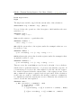
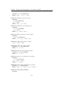
2.5
Expressions
typedef ’a WF_EXPRESSION =
"{f :: ’a WF_BINDING ⇒ ’a.
∃ t.
∀ b.
f(b) : t}"
Listing 3: Well-formed expressions
Expressions in Isabelle/UTP are, like predicates, implemented semantically.
An expression is a function from a binding to the valuation that the binding
yields. For instance the expression x + y would have be represented by the
binding function {{x 7→ 0, y 7→ 0} 7→ 0, {x 7→ 1, y 7→ 0} 7→ 1, {x 7→ 1, y 7→
1} 7→ 2 · · · }. We also require that expressions are well-typed and so each
18
D33.2b - Theorem Proving Support - Dev. Man. (Public)
binding must yield a value of the same type. The type of expressions is
defined in Listing 3.
We implement a variety of operators on expressions, a selection of which is
shown in Listing 4. The most interesting operator is substitution, which
we again implement semantically rather than syntactically. Specifically:
P [v/x] , {b | b(x := v(b)) ∈ P }. Effectively this says that a substitution
yields the set of bindings which, when x is assigned to the valuation of v
under b, yields a binding in P .
EqualP
:: α WF_EXPRESSION ⇒ α WF_EXPRESSION
⇒ α WF_PREDICATE
LitE
::
α ⇒ α WF_EXPRESSION
Op1E
::
(α ⇒ α) ⇒ (α WF_EXPRESSION ⇒ α WF_EXPRESSION)
Op2E
:: (α ⇒ α ⇒ α) ⇒ (α WF_EXPRESSION ⇒ α WF_EXPRESSION
⇒ α WF_EXPRESSION)
SubstP
:: α WF_PREDICATE ⇒ α WF_EXPRESSION
⇒ α VAR ⇒ α WF_PREDICATE
Listing 4: Expression operators
2.6
Relations and Imperative Programming
With the basic predicate theory mechanised, we can proceed to look at the
operators for sequential programming. In the UTP these are formalised as
binary relations, a subset of the predicates which consist only of undashed
and dashed variables, e.g. x, x0 , which are used to represent inputs and outputs, respectively. We define subsets for relations, preconditions and postcondition in Listing 5. These definitions require that the given predicate not
restrict any non-relational variables NON_REL_VAR for relations, and additionally DASHED or UNDASHED variables for preconditions and postconditions,
respectively.
The relational operators can now be described. Relational identity (the skip
operator) II is the set of bindings where all corresponding dashed and undashed variables are the same, i.e. II , {b. ∀x ∈ U. b(x0 ) = b(x)}. The
sequential composition operator is usually defined using an existential quantifier, for instance if α(P ) = v, v 0 then P # Q = ∃v0 .(P [v0 /v 0 ] ∧ Q[v0 /v]).
19
D33.2b - Theorem Proving Support - Dev. Man. (Public)
That is, the dashed variables from the P and the undashed variables from
Q are renamed so they correspond and then existentially quantified. In
Isabelle/UTP we implement this by means of permutations. Specifically:
P # Q , ∃D2 .(SS1 • P ∧ SS2 • Q), where SS1 maps dashed to doubly dashed
variables, SS2 maps undashed variables to doubly dashed variables and D2
is the set of doubly dashed variables.
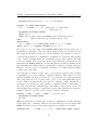
definition WF_RELATION :: "’a WF_PREDICATE set" where
"WF_RELATION = {p. UNREST NON_REL_VAR p}"
definition WF_CONDITION :: "’a WF_PREDICATE set" where
"WF_CONDITION = {p ∈ WF_RELATION. UNREST DASHED p}"
definition WF_POSTCOND :: "’a WF_PREDICATE set" where
"WF_POSTCOND = {p ∈ WF_RELATION. UNREST UNDASHED p}"
Listing 5: Well-formed relations, preconditions and postconditions
An assignment of an expression v to a variable x is implemented in a similar
way to relational identity: (x := v) , {b. ∀y ∈ D1 . b(y 0 ) = v(b) C x =
y B b(y 0 ) = b(y)}. For any variable y if x = y, then y 0 is given the value of v
under the binding, otherwise it is given the value of y, identifying.
2.7
Complete Lattices, Fixed-points and Iteration
The theory of lattices gives Isabelle/UTP a lattice ordering on predicates, and
the theory of complete lattices then provides the ability to define recursive
and iterative behaviours. The underlying order of the lattice is the refinement
order which is defined as closed reverse implication: P v Q , [Q ⇒ P ]. The
refinement order orders predicates by how deterministic they are.
As we have adopted a HOL set based implementation of predicates it is
possible to directly make use of the HOL implementation of lattice theory.
The underlying order on the lattice is, of course, the refinement order, but
at the level of sets this can be mapped onto the reverse subset relation ⊇.
Meet u then becomes ∨p and join t becomes ∧p . Top and bottom are false,
the miraculous predicate (which becomes {}), and true, the maximally nondeterministic predicate (which becomes UNIV), respectively. We can then
show that these operators form a bounded, distributive lattice.
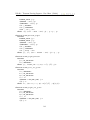
d
F
For complete lattices, we also need to define the infimum and supremum
S
T
operators, which internally map onto and , respectively, in the underlying
20
D33.2b - Theorem Proving Support - Dev. Man. (Public)
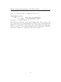
theorem Lattice_L1:
fixes P :: "’VALUE
WF_PREDICATE"
d
shows "P v
S ←→ (∀ X∈S. P v X)"
theorem Lattice_L2:
fixes Q :: "’VALUE WF_PREDICATE"
F
F
shows "( S) u Q =
{ P u Q | P. P ∈ S}"
theorem Lattice_L3:
fixes Q ::d "’VALUE WF_PREDICATE"
d
shows "(
S) t Q =
{ P t Q | P. P ∈ S}"
theorem Lattice_L4:
fixes Q ::d "’VALUE WF_PREDICATE"
d
shows "(
S) ; Q =
{ P ; Q | P. P ∈ S}"
theorem Lattice_L5:
fixes P :: "’VALUE
WF_PREDICATE"
d
d
shows "P ; (
S) =
{ P ; Q | Q. Q ∈ S}"
Listing 6: Complete Lattice laws
predicate model. This induces a complete lattice. Then, we derive the most
standard UTP complete lattice laws, a selection of which is shown in Listing
6.
Isabelle also has an implementation of Knaster-Tarski theorem, which states
that a monotonic function on a complete lattice induces a complete lattice of
fixed-points, and in particular there must be a least and greatest fixed-point.
Therefore, we directly make use of this to obtain the strongest fixed-point
ν and the weakest fixed-point µ. The standard fixed-point laws are then
derived, as shown in Listing 7. For instance, WFP_unfold states that if a
function over predicates F is monotone (mono F), then the fixed-point of this
function, µF, can be unfolded. This allows for predicates with recursion and
iteration.
Using the theory of complete lattices we can also demonstrate that UTP
predicates form a Kleene Algebra. A Kleene Algebra is an idempotent semiring with a star operator which is frequently used to reason about programs
with finite iteration. For the purposes of this work we use a comprehensive mechanisation of Kleene Algebra [ASW13b, ASW13a] in which a large
library of laws has been proved. The star operator is represented thusly:
21
D33.2b - Theorem Proving Support - Dev. Man. (Public)
theorem WFP: "F(Y) v Y =⇒ µ F v Y"
by (metis gfp_upperbound)
theorem WFP_unfold: "mono F =⇒ µ F = F(µ F)"
by (metis gfp_unfold)
theorem WFP_id: "(µ X · X) = true"
by (metis WFP top_WF_PREDICATE_def top_unique)
theorem SFP: "S v F(S) =⇒ S v ν F"
by (metis lfp_lowerbound)
theorem SFP_unfold: "mono F =⇒ F (ν F) = ν F"
by (metis lfp_unfold)
theorem SFP_id: "(ν X · X) = false"
by (metis SFP bot_WF_PREDICATE_def bot_unique)
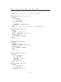
Listing 7: Fixed-point laws
d
P ? , n:N .P n , where P n is the result of running n copies of P in sequence.
The star is therefore a choice between all possible finite iterations of P . With
it we can specify a finite form of the while loop:
definition
IterP :: " ’a WF_PREDICATE
⇒ ’a WF_PREDICATE
⇒ ’a WF_PREDICATE" ("while _ do _ od")
where "IterP b P ≡ ((b ∧p P)? ) ∧p (¬p b0 )"
This definition is taken from Dexter Kozen’s paper on Kleene Algebra with
Tests [Koz97]. It effectively states that we consider all finite repetitions of P
where b remains true, each of which is terminated by b being false. We can
then prove some simple facts about loops.
theorem IterP_false: "while false do P od = II"
by (simp add:evalrr)
theorem IterP_true: "while true do P od = false"
by (simp add:evalrr)
The first states that an iteration with a false condition never executes; it
simply behaves as skip. The second states that an iteration with a true
22
D33.2b - Theorem Proving Support - Dev. Man. (Public)
condition never terminates; its behaviour is therefore miraculous, since a
finite iteration cannot represent infinite behaviours. This next proof is a
little more interesting.
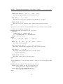
theorem IterP_unfold:
assumes "b ∈ WF_CONDITION" "S ∈ WF_RELATION"
shows "while b do S od = (S ; while b do S od) C b B II"
proof have "‘while b do S od‘ =
‘(while b do S od ∧ b) ∨ (while b do S od ∧ ¬b)‘"
by (metis AndP_comm WF_PREDICATE_cases)
also have "... = ‘((S ∧ b) ; while b do S od) ∨ (II ∧ ¬b)‘"
by (metis IterP_cond_false IterP_cond_true assms)
also have "... = (S ; while b do S od) C b B II"
by (metis AndP_comm CondR_def IterP_closure
SemiR_AndP_left_precond WF_CONDITION_WF_RELATION assms)
finally show ?thesis .
qed
Here we show that a while loop can be unfolded one step at a time. If the
condition is true then we obtain an execution of the body followed by the
while loop again, otherwise we obtain a skip. The proof is quite intuitive,
so it is shown. In the first step we split on the condition b which either be
true or false. In the second step we push the condition into both cases and
simplify. In the third step we rewrite the result as a conditional, completing
the proof. This is an example of a sledgehammer driven automated proof,
which we say more about in Section 2.9. A wider selection of laws about
iteration can be found in Appendix A.6. Additionally we have mechanised
the standard Hoare calculus law for partial correctness of loops which can be
found in Appendix A.7.
2.8
UTP Parser
Several of the UTP operators overlap with existing Isabelle syntax, and since
we’d like to maintain our own grammar for the UTP we implement a generic
parser. Isabelle supports mathematical symbols through the use of LATEX
like markup. For instance ∧ can be written as \<and>, ∀ can be written
as \<forall> and ∃ can be written as \<exists>. Moreover, Isabelle often
supports conversion of ASCII approximations into equivalent math symbols,
23
D33.2b - Theorem Proving Support - Dev. Man. (Public)
for instance ⇒ can be written as => and J can be written as [|. For more
information on Isabelle symbols please see the Isabelle Reference Manual,
Appendix B.
Isabelle also allows the construction of flexible mixfix parsers using its syntax
translation rules, by which a user can specify new non-terminals and build
production rules over these. This enables the construction of a parser for the
UTP which is extensible, in as much as new productions can be added (and
indeed deleted) at any time – ambiguities not withstanding. For instance the
UTP infix if-then-else operator can be specified in Isabelle as (infix ”_ C
_ B _”50), where 50 specifies the priority of the operator. The higher the
priority, the looser the operator binds.
The UTP parser uses a back-tick quoting notation, which augments Isabelle’s
own quoting system. Essentially this allows the user to write predicate syntax
as they would expect for the UTP, including predicate operators, relational
operators, imperative programming constructs and a variety of expressions.
Some examples of UTP predicates written using this syntax are shown below.
term "‘(P ∧ Q) ⇒ P‘"
term "‘(P C b B Q)‘ v ‘(b ∧ P)‘"
term "‘$x ∈ {« 1» ,« 2» ,« 3» } v $x = « 2» ‘"
term "‘x := (« 7» * $z) ; ((y := $x + « 1» ) C ($x < « 10» ) B P)‘"
The parser is built on two main grammar levels: predicates and expressions,
though for the most part this distinction may not be seen. Essentially, things
like P ∧ Q, II or P; Q are predicates, whilst things like $x + $y are expressions.
For instance, in the predicate ‘x := v ; P‘, v is an expression and P is a
predicate.
The dollar notation, e.g. $x, refers to UTP variables, which can either be
program variables or auxiliary variables. These variables denote values which
may be observed in a predicate. Several other types of variables may exist
in a terms, for instance HOL variables can be used to denote predicates or
expressions, for instance in specifying algebraic laws. UTP variables may
be dashed to represent outputs by using the \<acute> Isabelle symbol, e.g.
$x0 .
Guillemots (« ») are used to denote literal HOL terms, and essentially any
HOL value or expression may be encapsulated. The only proviso is that
24
D33.2b - Theorem Proving Support - Dev. Man. (Public)
suitable mappings are defined in the underlying value model.
2.9
Automated Proof
Isabelle/UTP would be of limited use if proofs can only be constructed by
experts. Clearly the focus of the theorem proving plugin in the COMPASS
tool is on automated proof, with manual proof available only as a last resort.
The problem often associated with deep-embeddings is that they often cannot directly make use of existing proof strategies in an ITP. Ease of proof
is sacrificed for accuracy in the encoding. Isabelle/HOL has a wide variety of proof tools available, so the question is how to make use of these in
Isabelle/UTP?
The solution to this problem is proof by interpretation, lifting and transfer [HK12]; well known techniques in the theorem proving world. Rather
than directly performing proof on the new domain, suitable sub-calculi from
within this domain are identified and problems which exist entirely within the
domain can be transferred to a different domain for which well-known proof
procedures exists. For example the predicate operators in Isabelle/UTP all
have corresponding constructs in HOL predicates, and of course HOL predicates can make use of tactics likes auto and sledgehammer [BBN11]. Therefore
we can transfer problems written using only the UTP predicate operators into
the HOL domain and vastly improve proof potential. Similarly the relational
calculus operators all have analogues in the world of HOL binary relations,
and a large library of laws for reasoning about HOL relations has already
been established. This problem is alleviated by the semi-shallow nature of
Isabelle/UTP, in particular use of HOL sets to encode predicates. Therefore
we have a way for mechanising proof in the UTP, and therefore by extension
CML.
A proof tactic in Isabelle/UTP consists of three parts:
1. interpretation function – this maps elements of a UTP theory to elements of a target domain, in which we desire to perform the proof;
2. transfer rules – these show how results in the target domain map to
results in the UTP theory;
3. congruence rules – map operators from the signature of the UTP theory
to operators in the target domain.
Such proof tactics are always partial – they apply only to the operators of
the theory. For instance our predicate tactic, utp-pred-tac, can only solve
25
D33.2b - Theorem Proving Support - Dev. Man. (Public)
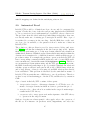
Interpretation Function
EvalP :: α WF_PREDICATE ⇒ α WF_BINDING ⇒ bool (J_K_)
Transfer Theorem
(P = Q) ←→ (∀b.JP Kb = JQKb)
Congruence Rules (Selection)
JtrueKb
JfalseKb
J¬p P Kb
JP ∧p QKb
J∃p vs. pKb
F
J psKb
=
=
=
=
=
=
True
False
¬JP Kb
JP Kb ∧ JQKb
∃b0 .JP K(b ⊕ b0 on vs)
(∀p ∈ ps.JpKb)
Table 1: utp-pred-tac: Transfer function and rules
problems built using the predicate operators. Similarly, our relational tactic,
utp-rel-tac can only solve problems in relational calculus. The algorithm for
performing proof using these tactics is usually of this form:
1. Apply a transfer rule to the proof goal (for a suitable target
model).
2. Apply the associated congruence rules, to interpret the UTP theory operators into operators of the target domain. This process need
not be complete, and subterms outside the theory will remain uninterpreted. So long as the proof does not depend on the uninterpreted
constants it can still succeed.
3. Apply a builtin HOL tactic, for instance simp, auto or sledgehammer.
This algorithm is, for the most part all-or-nothing – if the HOL tactic cannot
solve the interpreted goal the user will be left with a partially interpreted
term of the target theory where the details of the encoding are exposed. This
is an undesirable situation as the user may not be able to comprehend the
meaning of this term. We will alleviate this problem later. First we explore
the tactics developed so far.
utp-pred-tac is a tactic for interpreting the UTP predicate operators into the
HOL predicate operators. The interpretation function and associated rules
can be seen in Table 1. It works by converting an equality on predicates
26
D33.2b - Theorem Proving Support - Dev. Man. (Public)
P and Q into the tautology that under any binding b, P and Q evaluate
to the same boolean valuation. The congruence rules convert the predicate
operators in the expected way. UTP true becomes HOL True, ∧p becomes ∧
and so on. The only really complicated operator is the existential quantifier
which cannot be directly mapped to the HOL existential (since we handle
variables in a deep way) and instead becomes a function override. With this
tactic we can prove many of standard laws of predicates, such as for instance
that they form a Boolean Algebra. A selection of laws is proved below.
theorem AndP_comm :
"p1 ∧p p2 = p2 ∧p p1"
by (utp_pred_auto_tac)
theorem AndP_OrP_distr:
"(p1 ∨p p2) ∧p p3 = (p1 ∧p p3) ∨p (p2 ∧p p3)"
by (utp_pred_auto_tac)
theorem OrP_excluded_middle :
"p ∨p ¬p p = true"
by (utp_pred_tac)
theorem Demorgan1: "¬p (x ∨p y) = ¬p x ∧p ¬p y"
by (utp_pred_auto_tac)
theorem NotP_NotP: "¬p ¬p p = p"
by (utp_pred_tac)
We have used utp-pred-tac to prove over 100 such laws. Nevertheless, what
the predicate tactic cannot do is solve conjectures over the relational operators (or indeed over operators from other theories). Therefore we need
additional tactics. utp-rel-tac and utp-xrel-tac are tactics for discharging relational calculus conjectures. They both map UTP predicates into a form of
HOL relation, which means that the preexisting laws for HOL relations can
be applied in proofs.
The difference between the two tactics is how variable bindings are represented in the underlying target model, and in particular how they handle
non-relational variables (e.g. doubly dashed variables). utp-rel-tac preserves
them, so that goals which may involve non-relational variables can be discharged. However this means that several UTP relational operators cannot
be mapped to equivalents in HOL. In particular the tactic cannot handle the
true and ¬_ operators, since for instance relational complement negates only
27
D33.2b - Theorem Proving Support - Dev. Man. (Public)
relational variables, but predicate complement negates all variables. Nevertheless, laws such as associativity can be proved by utp-rel-tac, and without
any assumptions, making it a useful tactic.
In contrast, utp-xrel-tac can only solve conjectures over well-formed relations,
i.e. elements of WF_RELATION. However, it can handle all the operators of
relational calculus, and is a much more powerful tactic. Therefore it largely
depends on the form of the goal for which of these tactics should be applied.
Interpretation Function
EvalR :: α WF_PREDICATE ⇒ (α WF_REL_BINDING) rel (J_KR)
Transfer Theorems
(P = Q) ←→ (JP KR = JQKR)
(P v Q) ←→ (JP KR ⊇ JQKR)
P, Q ∈ WF_RELATION =⇒ (P = Q) ←→ (JP KRX = JQKRX )
P, Q ∈ WF_RELATION =⇒ (P v Q) ←→ (JP KRX ⊇ JQKRX )
Congruence Rules (Selection)
JfalseKR
JP ∧p QKR
JP ∨p QKR
JIIKR
JP # QKR
JP 0 KR
JP n KR
JP ? KR
=
=
=
=
=
=
=
=
∅
JP KR ∩ JQKR
JP KR ∪ JQKR
Id
JP KR ◦ JQKR
(JP KR)−1
(JP KR) ∧∧ n
(JP KR)∗
JtrueKRX = UNIV
J¬P KRX = − (JP KRX )
Table 2: utp-rel-tac/utp-xrel-tac: Transfer function and rules
The interpretation function and rules for utp-rel-tac and utp-xrel-tac are
shown in Table 2. All the congruence rules for utp-rel-tac apply for utp-xreltac (modulo closure properties) and therefore only the difference is shown.
The mapping is mainly intutive; false maps to the empty relation ∅, ∧p maps
to ∩, skip II maps to relational identity Id and sequential composition #
maps to relation composition ◦. For utp-xrel-tac, true maps to the universe
set UNIV and ¬ maps to relational complement −.
28
D33.2b - Theorem Proving Support - Dev. Man. (Public)
Additionally, we provide mappings for some of the more interesting operators. A primed relation can be represented by relational converse − 1, which
is particularly useful for reasoning about preconditions, since converse then
corresponds to conversion to a postcondition. We also map the power operator P n , and use this to map the Kleene Star operator, which becomes
the reflective-transitive closure operator in relation algebra. This aids in automating proofs about iteration. A selection of laws proved using utp-rel-tac
and utp-xrel-tac is shown below.
theorem SemiR_OrP_distl :
"P1 ; (P2 ∨p P3) = (P1 ; P2) ∨p (P1 ; P3)"
by (utp_rel_auto_tac)
theorem SemiR_SkipR_left [simp]:
"II ; P = P"
by (utp_rel_auto_tac)
theorem SemiR_FalseP_left [simp]:
"false ; P = false"
by (utp_rel_auto_tac)
theorem SemiR_assoc :
"P1 ; (P2 ; P3) = (P1 ; P2) ; P3"
by (utp_rel_auto_tac)
theorem SemiR_TrueP_compl [simp]:
assumes "P ∈ WF_RELATION"
shows "¬p (P ; true) ; true = ¬p (P ; true)"
using assms by (utp_xrel_auto_tac)
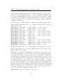
With these tactics we have built a large library of algebraic laws about predicates and relations. At time of writing this stood at over 300. For a large
selection of these laws, see the law catalogue in Appendix A, sections A.1
and A.2.
The algebraic laws provide an additional way of performing automated proof
using sledgehammer. Sledgehammer complements the UTP tactics by making
powerful equational and first-order reasoning available, which the tactics do
not necessarily excel at. For instance we can prove the following law using a
mixed algebraic / tactical approach. The unreachable branch law shows that
if we have an if-statement embedded within an if-statement, both with the
same condition, then the inner then-branch cannot be reached.
29
D33.2b - Theorem Proving Support - Dev. Man. (Public)
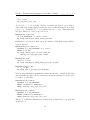
theorem CondR_unreachable_branch:
"‘(P C b B (Q C b B R))‘ = ‘P C b B R‘" (is "?lhs = ?rhs")
proof have "?lhs
= ‘((Q C b B R) C ¬b B P)‘"
by (metis CondR_sym)
also have "... = ‘(Q C b ∧ ¬ b B (R C ¬ b B P))‘"
by (metis CondR_assoc)
also have "... = ‘(Q C false B (R C ¬ b B P))‘"
by (utp_pred_tac)
also have "... = ‘(R C ¬ b B P)‘"
by (metis CondR_false)
also have "... = ?rhs"
by (metis CondR_sym)
finally show ?thesis .
qed
There are five steps to the proof. Four of them are discharged by application
of sledgehammer, indicated by the metis keyword applied to a list of algebraic laws. One of them is discharged by utp-pred-tac, indicating the use of
predicate calculus reasoning. The tactics are much faster to apply and are
very good at proofs which can be done by simplification, where sledgehammer
performs much better when, for instance, additional terms must be inserted
in a proof-step.
2.10
Supporting theorems and attributes
Algebraic laws often require supporting proofs, for instance proof about relations will often assume that predicates are well-formed relations, i.e. members of the set WF_RELATION. A law which shows membership of such a set
is called a closure law. For instance:
JP ∈ WF_RELATION; Q ∈ WF_RELATIONK =⇒ P; Q ∈ WF_RELATION
This laws states that sequential composition is closed under well-formed relations. Similarly –
Jx ∈ UNDASHEDK =⇒ VarP x ∈ WF_CONDITION
– states that a predicate variable x forms a precondition provided that x is
an undashed variable. We group together laws of this form under a theorem
30
D33.2b - Theorem Proving Support - Dev. Man. (Public)
attribute called closure. Theorem attributes are used to group similar laws
together such that, for instance, they can easily be invoked to try and prove
closure of a composite predicate.
In Isabelle/UTP we create a variety of such theorem attributes for proving
different properties. The most notable ones are listed below.
• closure – used to prove that a predicate is contained in a given set,
e.g. WF_CONDITION, WF_DESIGN. Provides a coarse form of typing for
predicates.
• unrest – unrestriction theorems. Show which variables are unrestricted
in a given operator. e.g. UNREST (− {x}) (VarP x)
• typing – value typing introduction laws.
e.g. Jx : Z; y : ZK =⇒ (x + y) : Z.
• defined – definedness theorem, e.g. D(x/0) = False
• erasure – type erasure theorems. Used to convert between shallow
values / expressions, and their deep equivalents.
e.g. (x + y) ↓ = x ↓ +N y ↓.
• urename – renaming / permutation theorems. Show the effect of applying a permutation to a given predicate / expression.
e.g. ([x 7→ y] • x) = y
• usubst – substitution theorems. Show the effect of substituting a given
expression into a predicate or expression.
e.g. (P ∧ Q)[v/x] = P[v/x] ∧ Q[v/x]
• eval – transfer and congruence theorems associated with utp-pred-tac
• evalr – transfer and congruence theorems associated with utp-rel-tac
• evalrx – transfer and congruence theorems associated with utp-xrel-tac
These theorem attributes can be given to the Isabelle simplifier to solve a
goal of the correct form. Some of the theorem attributes are dependent on
others. For instance some substitution theorems in usubst need to show that
a variable can accommodate a given expression, and therefore typing and
defined are often required too.
Theorem sets can be augmented with user-supplied theorems by adding a
theorem attribute annotation after the theorem name, for instance:
theorem EvalP_ImpliesP [eval]: "[[p1 ⇒p p2]]b = ([[p1]]b −→ [[p2]]b)"
31
D33.2b - Theorem Proving Support - Dev. Man. (Public)
This creates the utp-pred-tac evaluation theorem for implies and adds it to
the eval theorem set. In this way the user can extend the various tactics
with their own congruence laws, for instance when defining their own UTP
operators. Often, if these operators are defined only in terms of pre-existing
UTP operators, the definitional equation for the operator can be added to the
evaluation theorems. Similarly, closure laws, unrestriction laws, substitution
laws and renaming laws may all be desired for the new operators, in which
case the user must specify, prove, and add them to the appropriate theorem
set. This is exemplified in our mechanisation of the theory of designs in
Section 3.
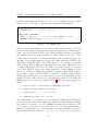
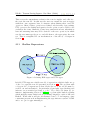
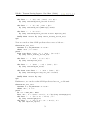
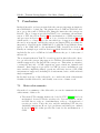
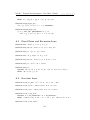
2.11
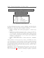
Shallow Expressions
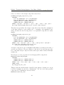
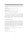
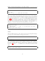
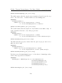
Figure 2: Relating HOL types and UTP types
Isabelle/UTP supports a shallow model of expressions, which is built on top
of the core expression model presented in Section 2.5. The problem with
a deep model of expressions is that all the theory of the model must be
worked out and mechanised. In particular polymorphic type-checking and
inference are non-trivial problems to solve. We could solve them by, for
instance, implementing System F [GTL89], a polymorphic lambda calculus
which underlies many functional programming languages, such as ML and
Haskell. While this would give us maximal control of our language, time
constraints prevent us from implementing the type inference system of CML
and so we opt for approximating it.
32
D33.2b - Theorem Proving Support - Dev. Man. (Public)
Our shallow model of expressions adopts the HOL type system for type
checking and inference. A type system implemented in this way cannot go
beyond the expressivity of HOL and therefore can’t support more advanced
features like union types or dependent types. This is not a fundamental
limitation of Isabelle/UTP itself which internally can support any form of
typing which can be described using the type relation. Rather, we choose
to limit ourselves so that we gain ease of proof through HOL’s own type
system, function library and associated proven facts. This limitation could
be lifted in future work by a more precise implementation of the CML type
system.
We provide a thin layer which links a suitable subset of HOL types to UTP
types in the predicate model. The types we have implemented so far are
polymorphic in a single parameter which represents the underlying value
model, e.g. α VAR, α WF_PREDICATE and α WF_EXPRESSION. They carry
no type information about the data contained within (although predicates
are effectively always boolean valued). This is to some extent deliberate, for
example having no type data means we can compare two values of different
types, which would be impossible if we carried type data.
Nevertheless, in many situations it is very convenient to carry this data
around, for instance for the purpose of type inference. Therefore we define parallel concepts which, in addition to the type variable referring to the
model type, also carry a type variable referring to the type of data within.
However, this raises a problem – how do we relate the underlying value domain with HOL types? This is a particular troublesome problem as HOL
type classes may not range over two type variables. The solution is to create
three polymorphic constants, InjU, ProjU and TypeU to act as injection, projection and type mapping functions, respectively, between the value domain
and HOL types.
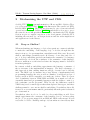
The idea is illustrated in Figure 2. We identify a region of our value domain
which corresponds to a HOL type α. Functions InjU and ProjU allow mapping to and from this region. Most important is the function TypeU which
effectively maps a HOL type to a UTP type. Intuitively, we would like the
constraint that v :: α ←→ InjU(v) : TYPEU(α), though this is impossible to
encode within HOL.
With the ability to map between HOL types and UTP types in place, we
begin to encode the various polymorphic UTP concepts. We begin with
variables, which are shown in Listing 8. A polymorphic variable carries two
parameters, the first giving the type of the variable and the second of the
underlying value domain. Internally a polymorphic variable consists of a
33
D33.2b - Theorem Proving Support - Dev. Man. (Public)
typedef (’a, ’m :: VALUE) PVAR = "UNIV :: (NAME * bool) set"
definition PVAR_VAR :: "(’a, ’m) PVAR ⇒ ’m VAR" where
"PVAR_VAR v = MkVar (pvname v) (TYPEU(’a)) (pvaux v)"
Listing 8: Polymorphic variables
name and auxiliary flag, similar to a core variable. The two type variables
are not referenced as they are simply present for typing and perform no other
function. We also defined a function PVAR_VAR which converts a polymorphic
variables to a core variable. This operator technically performs type erasure
– it converts the parametrised HOL type to a UTP type, which is stored
inside the core variable, and then discards the type information present in
’a. Type erasure operators like this are given special syntax: x ↓, where x
is any polymorphic constant (e.g. a PVAR).
One could ask, why have two kinds of variable type? Could we replace VAR
entirely by PVAR and always carry type data around? The answer is no,
because we then could not talk about a set of variables (e.g. an alphabet),
because HOL sets are monomorphic. Indeed all HOL collection types can
only refer to a single type, and therefore to talk about collections of heterogeneously typed things we must first apply type erasure. Thus reasoning
at the two levels, core and polymorphic, or deep and shallow, is necessary.
Reasoning about programming language semantics is usually easier at the
deep level, whilst reasoning about programs is usually easier at the shallow
level.
A polymorphic expression is then implemented, similar to a core expression,
as a function from bindings to a value of type ’a, as illustrated in Listing
9. Bindings themselves cannot be reimplemented polymorphically, as this
would require dependent function types which HOL cannot support. Instead
we use type erasure to marshal data between the deep and shallow levels.
To exemplify we give the definition of three operators. LitPE lifts a HOL
value to a literal expression. It is implemented as the constant function
which returns the desired literal for any binding. VarPE performs a variable
lookup. It first erases the variable, looks up the value of this variable in the
binding, and then projects the UTP value to a HOL value. So long as the
correspondance between HOL types and UTP types follows, this lookup will
produce a correctly typed value. Op1PE lifts a HOL function to an operator
on expressions. It is implemented as the binding function which applies the
function f to the value of the each possible value of u.
34
D33.2b - Theorem Proving Support - Dev. Man. (Public)
typedef (’a, ’m) WF_PEXPRESSION
= "UNIV :: (’m WF_BINDING ⇒ ’a) set"
morphisms DestPExpr MkPExpr
notation DestPExpr ("[[_]]∗ ")
definition LitPE :: "’a ⇒ (’a, ’m) WF_PEXPRESSION"
where "LitPE v = MkPExpr (λ b. v)"
definition VarPE :: "(’a, ’m) PVAR ⇒ (’a, ’m) WF_PEXPRESSION"
where "VarPE x = MkPExpr (λ b. ProjU (hbib x↓))"
definition Op1PE ::
"(’a ⇒ ’b) ⇒
(’a, ’m) WF_PEXPRESSION ⇒ (’b, ’m) WF_PEXPRESSION"
where "Op1PE f u = MkPExpr (λ b. f ([[u]]∗ b))"
Listing 9: Polymorphic expressions
Polymorphic expressions thus implemented, we can now use the HOL typesystem to aid in reasoning about UTP predicates.
2.12
Channels and Events
Events are an important concept in the UTP, particularly with regard to the
theory of reactive processes and CSP. Clearly then they are also important for
CML in that they give us the basis for talking about communications between
constituent systems. We provide a number of datatypes for reasoning about
channels in the core Isabelle/UTP library.
Events can carry data, and therefore channels are represented as name/type
pairs. As for all other UTP types, channels are parametric over the value
domain type ’a.
typedef ’a UCHAN = "UNIV :: (NAME * ’a UTYPE) set"
morphisms DestUCHAN MkUCHAN
by (simp)
An event then is a pairing of a channel and a value of the correct type, though
we need some additional infrastructure too.
class EVENT_PERM = VALUE +
fixes
EventPerm :: "’a UTYPE set"
35
D33.2b - Theorem Proving Support - Dev. Man. (Public)
assumes EventPerm_exists: "∃ x. x ∈ EventPerm"
typedef (’m::EVENT_PERM) EVENT =
"{(c :: ’m UCHAN, v :: ’m). uchan_type c ∈ EventPerm
∧ v : uchan_type c}"
morphisms DestEVENT MkEVENT
apply (auto)
apply (metis (mono_tags) DestUCHAN_cases EventPerm_exists
UNIV_I default_type snd_def split_conv)
done
abbreviation
EV :: "NAME ⇒ (’a::EVENT_PERM) UTYPE ⇒ ’a ⇒ ’a EVENT"
where "EV n t v ≡ MkEVENT (MkUCHAN (n, t), v)"
We create a sort type-class called EVENT_PERM which describes the set of
permissible event types. The rationale for this is that not all value models
may support all kinds of types for use in channels. For instance it may be
considered nonsensical to communicate an infinite set. This class then defines
a set of types in EventPerm, the permissible types, and requires that this
set be non-empty. The event type then requires that the parametric model
instantiate the EVENT_PERM type. It specifies that an event is a channel/value
pair such that the channel type is a permissible event type and the value has
this type. We also create a convenient constructor for events called EV, taking
a name, type and value.
An event type is a kind of sigma type or existentially quantified type, in that
it quantifies over a type which is otherwise hidden. This cannot be done
directly in HOL, the type would need to be referenced in a type-parameter
and could therefore not be placed into a list or set with differently typed
events. This would means the trace model couldn’t be built, and therefore
is another reason why we cannot build a completely shallow embedding of
the UTP. Nevertheless, with the help of the shallow expression model we can
use the HOL type-system to check that a given value matches its respective
channel. Therefore we also create a type for shallow channels.
typedef ’a CHAN = "UNIV :: (NAME * ’a itself) set"
morphisms DestCHAN MkCHAN
by simp
CHAN is parametrised over the type of value it communicates. If the said type
is injectable into a suitable value model then this type is isomorphic with
UCHAN. We then create a polymorphic expression constructor for events.
definition PEV :: "’a CHAN ⇒ ’a ⇒ (’m :: EVENT_SORT) EVENT" where
36
D33.2b - Theorem Proving Support - Dev. Man. (Public)
"PEV c v = EV (chan_name c) TYPEU(’a) (InjU v)"
abbreviation EventPE ::
"’a CHAN ⇒ (’a, ’m :: EVENT_SORT) WF_PEXPRESSION
⇒ (’m EVENT, ’m) WF_PEXPRESSION" where
"EventPE n v ≡ Op1PE (PEV n) v"
PEV builds an event from a polymorphic channel and a value of the correct
type, using injection and typing functions for HOL values. EventPE lifts this
function to an expression. Notice that both of these function perform typeerasure – the type of the channel disappears in the output type. This then
allows the construction of channels, events, and sets thereof.
37
D33.2b - Theorem Proving Support - Dev. Man. (Public)
3
Mechanising a UTP theory
In this section we will demonstrate how to mechanise a theory in UTP, using
the Theory of Designs [HJ98, Chapter 3] to exemplify. A UTP theory is
a meta-theoretic entity which is used to formalise part of the underlying
semantics of a specification or programming language like CML. The proofs
are therefore not about a specific program, but about the language itself.
Nevertheless having a consistent semantics is important to ensure that proofs
about the programs are themselves meaningful. Many of the laws which we
prove in this Section can then be safely applied to program verification. Proof
in concrete CML specifications is dealt with in Section 4 and exemplified in
Section 6.
A theory in the UTP consists of three things:
1. an alphabet – the observations which can be made on objects of the
theory;
2. a signature – the functions on objects of the theory;
3. healthiness conditions – under which the objects of the theory are closed
We will look at these one by one.
3.1
Design Alphabet
The theory of designs uses the boolean variable ok and ok 0 to indicate
that a program has successfully started and successfully terminate, respectively.
abbreviation
"okay ≡ MkPlainP ’’okay’’ True TYPE(bool) TYPE(’m :: BOOL_SORT)"
We formalise okay in Isabelle/UTP by means of the MkPlainP function, which
takes a string, auxiliary flag, HOL type and model. okay is an auxiliary
variable, meaning it has no meaning for the program itself but only for its
structure. Auxiliary variables must also always be defined. The model variable 0 m essentially defines the constraints which must be imposed on value
models which desire to implement a theory. In the case of designs we only
require booleans, which are axiomatised through the class BOOL_SORT. The
primed version okay 0 can be obtained simply by applying the prime function
to okay.
Since most design predicates need a boolean type, we also set the appropriate
38
D33.2b - Theorem Proving Support - Dev. Man. (Public)
sort constraint:
default_sort BOOL_SORT
This means that all future defined syntax will implicitly impose the BOOL_SORT
constraint.
3.2
Design Signature
The signature of the theory consists of all the operators which act to construct and otherwise manipulate designs. We first set up some useful abbreviations.
abbreviation "ok ≡ ‘$okay‘"
abbreviation "ok’ ≡ ‘$okay0 ‘"
abbreviation "OKAY ≡ {okay↓,okay↓0 }"
To make writing predicates a little more concise we set up the predicates ok
and ok 0 , and the set {okay↓, okay↓0 } which contains these two variables, and
effectively defines the minimal design alphabet. Next we start to define the
design operators.
definition DesignD ::
"’a WF_PREDICATE ⇒
’a WF_PREDICATE ⇒
’a WF_PREDICATE" (infixr "`" 60) where
"P ` Q = ‘ok ∧ P ⇒ ok’ ∧ Q‘"
The design turnstile ` is a binary operator on predicates, the first predicate is
the assumption of the design, and the second is the commitment of the design
– what it must achieve if its assumption is satisfied. ok is true only when
the assumption is satisfied, and ok 0 only when the commitment is reached.
Notice the use of backtick quotes in the definition – this indicates the use of
the UTP parser rather than the HOL parser.
definition SkipD :: "’a WF_PREDICATE" ("IID ") where
"SkipD = true ` IIREL_VAR - OKAY "
IID is a design whose assumption is true, and commitment is relational
identity on all relational variables (indicated by REL_VAR), other than those
in {okay↓, okay↓0 } which are of course taken care of by the turnstile.
definition BotD :: "’a WF_PREDICATE" ("⊥D ") where
"BotD = true"
39
D33.2b - Theorem Proving Support - Dev. Man. (Public)
definition TopD :: "’a WF_PREDICATE" (">D ") where
"TopD = (¬p ok)"
Next we define the top and bottom of the design lattice. ⊥D is the same as
for the normal predicate lattice, i.e. true. >D is ¬ok, since false is, as we
shall see, not closed under the design healthiness conditions.
definition J_pred :: "’a WF_PREDICATE" ("J") where
"J ≡ (ok ⇒p ok’) ∧p IIREL_VAR - OKAY "
The idempotent predicate J will be used in the definition of H2 and its
subsequent proofs. We will say more about this later.
abbreviation ok_true ::
"’a WF_PREDICATE ⇒ ’a WF_PREDICATE" ("_t " [1000] 1000) where
"pt ≡ ‘p[true/okay0 ]‘"
abbreviation ok_false ::
"’a WF_PREDICATE ⇒ ’a WF_PREDICATE" ("_f " [1000] 1000) where
"pf ≡ ‘p[false/okay0 ]‘"
We also set up the usual convenient syntax for substitution ok 0 for true and
false respectively. These functions effectively extract the commitment (under
the assumption) and the negated assumption, respectively.
definition ParallelD ::
"’a WF_PREDICATE ⇒
’a WF_PREDICATE ⇒
’a WF_PREDICATE" (infixr "k" 100) where
"P k Q = (¬p Pf ∧p ¬p Qf ) ` (Pt ∧p Qt )"
For the sake of completeness, we also define the design parallel composition operator. It conjoins the assumptions of the two designs (which are
extracted by substituting ok 0 for false and negating), and conjoins the two
commitments. At this point we are still using the HOL parser for our terms,
which is why everything has p subscripts. This requirement will be alleviated
shortly.
declare
declare
declare
declare
declare
BotD_def [eval,evalr,evalrx]
TopD_def [eval,evalr,evalrx]
DesignD_def [eval,evalr,evalrx]
J_pred_def [eval,evalr,evalrx]
SkipD_def [eval,evalr,evalrx]
40
D33.2b - Theorem Proving Support - Dev. Man. (Public)
declare ParallelD_def [eval,evalr,evalrx]
We now add all the definitional equations for our operators to the various
tactics, namely utp-pred-tac, utp-rel-tac and utp-xrel-tac. This will enable the
tactics to solve goals using our new operators.
syntax
"_upred_desbot"
"_upred_destop"
"_upred_design"
"_upred_ok_true"
"_upred_ok_false"
"_upred_SkipD"
"_upred_J"
"_upred_parallel"
::
::
::
::
::
::
::
::
"upred" ("⊥D ")
"upred" (">D ")
"upred ⇒ upred ⇒ upred" (infixr "`" 30)
"upred ⇒ upred" ("_t " [1000] 1000)
"upred ⇒ upred" ("_f " [1000] 1000)
"upred" ("IID ")
"upred" ("J")
"upred ⇒ upred ⇒ upred" (infix "k" 50)
translations
"_upred_desbot"
"_upred_destop"
"_upred_design p q"
"_upred_ok_true p"
"_upred_ok_false p"
"_upred_SkipD"
"_upred_J"
"_upred_parallel P Q"
==
==
==
==
==
==
==
==
"CONST
"CONST
"CONST
"CONST
"CONST
"CONST
"CONST
"CONST
BotD"
TopD"
DesignD p q"
ok_true p"
ok_false p"
SkipD"
J_pred"
ParallelD P Q"
Finally we extend the UTP parser with all our new syntax, by adding new
syntax nodes and translation rules to the AST. For details of how this works
please refer to Isabelle 2013 reference manual, Section 7.5.2.
3.2.1
Unrestriction and Closure theorems
In this section we set up some useful lemmas, which will make later proofs
easier. UNREST theorems are rules which show that certain variables are not
referred to in particular operators – effectively these are "fresh" variables, or
variables which are not in the implicit alphabet.
lemma UNREST_DesignD [unrest]:
"[[ UNREST vs P; UNREST vs Q; okay↓ ∈
/ vs; okay↓0 ∈
/ vs ]]
=⇒ UNREST vs (P ` Q)"
by (simp add:DesignD_def unrest)
The lemma above, for instance, shows that if both the assumption P and
41
D33.2b - Theorem Proving Support - Dev. Man. (Public)
commitment Q of a design are unrestricted by the variables in vs, and neither
okay nor okay 0 are in vs then likewise P ` Q is not restricted by vs. Similar
theorems exist for the other design operators.
lemma TopD_rel_closure [closure]:
">D ∈ WF_RELATION"
by (simp add:TopD_def closure)
lemma DesignD_rel_closure [closure]:
"[[P ∈ WF_RELATION; Q ∈ WF_RELATION]] =⇒ P ` Q ∈ WF_RELATION"
by (simp add:DesignD_def closure)
lemma SkipD_rel_closure [closure]:
"IID ∈ WF_RELATION"
by (auto intro:closure simp add:SkipD_def)
Closure theorems define that particular operators are closed under particular
UTP theories. In this case we show that several of the design operators are
closed under relations, as expected.
3.2.2
Algebraic Laws
With the new operators defined and some basic properties about them proved
we proceed to prove some of the major results about designs. For completeness, mechanised proofs for all these properties are shown. However, understanding their structure is not necessary for understanding the general
principles of mechanising a theory.
theorem DesignD_extreme_point_true_1:
"false ` false = false ` true"
proof have "‘false ` false‘ = ‘ok ∧ false ⇒ ok’ ∧ false‘"
by (simp add:DesignD_def)
also have "... = ‘false ⇒ ok’ ∧ false‘"
by simp
also have "... = ‘true‘"
by simp
also have "... = ‘false ⇒ ok’ ∧ true‘"
42
D33.2b - Theorem Proving Support - Dev. Man. (Public)
by simp
also have "... = ‘ok ∧ false ⇒ ok’ ∧ true‘"
by simp
also have "... = ‘false ` true‘"
by (simp add:DesignD_def)
finally show ?thesis .
qed
This first law shows that false ` false and false ` true are the same.
In fact both of these predicates are equal to true, the bottom of the design
lattice. As this is the first proof in the section we proceed step-by-step
using the Isar proof scripting language. The proof is actually quite easy,
and basically involves showing that both terms can be written in the form
f alse ⇒ p, which is true. Such easy proofs need not be explicitly elucidated
though.
theorem DesignD_extreme_point_true:
"false ` false = false ` true"
"false ` true = true"
by (utp_pred_tac+)
theorem DesignD_extreme_point_nok:
"true ` false = ¬p ok"
"¬p ok = >D "
by (utp_pred_tac+)
This result goes through easily by utp-pred-tac. Similarly, we can show that
¬ok can be written as the design true ` false.
theorem DesignD_assumption:
assumes "UNREST OKAY P"
shows "‘¬ (P ` Q)f ‘ = ‘P ∧ ok‘"
using assms by (utp_pred_auto_tac)
theorem DesignD_commitment:
assumes
"UNREST OKAY P"
"UNREST OKAY Q"
shows "‘(P ` Q)t ‘ = ‘(ok ∧ P ⇒ Q)‘"
using assms by (utp_pred_auto_tac)
43
D33.2b - Theorem Proving Support - Dev. Man. (Public)
Next, we can show that the assumption and commitment of a design can
indeed by extracted by application of ¬_f and _t , respectively. These results
follow only when P and Q do not talk about ok and ok 0 . We solve them by
a variant of utp-pred-tac called utp-pred-auto-tac, which additionally uses the
auto tactic. This is needed due the presence of a non-trivial implication
statement.
theorem DesignD_export_precondition:
"‘P ` Q‘ = ‘P ` P ∧ Q‘"
by (utp_pred_tac)
This law shows that the precondition of a design may be imported into the
post condition. It follows easily from a similar fact for implication.
We now have our first long proof: the design refinement law.
theorem DesignD_refinement:
assumes
"UNREST OKAY P1"
"UNREST OKAY P2"
"UNREST OKAY Q1"
"UNREST OKAY Q2"
shows "P1 ` Q1 v P2 ` Q2 = ‘[P1 ⇒ P2] ∧ [P1 ∧ Q2 ⇒ Q1]‘"
proof have "‘(P1 ` Q1) v (P2 ` Q2)‘ = ‘[P2 ` Q2 ⇒ P1 ` Q1]‘"
by (utp_pred_tac)
also
have "... = ‘[(ok ∧ P2 ⇒ ok’ ∧ Q2) ⇒ (ok ∧ P1 ⇒ ok’ ∧ Q1)]‘"
by (utp_pred_tac)
also from assms
have "... = ‘[(P2
apply (rule_tac
apply (rule_tac
apply (simp_all
done
⇒ ok’ ∧ Q2) ⇒ (P1 ⇒ ok’ ∧ Q1)]‘"
trans)
x="okay↓" in BoolType_aux_var_split_taut)
add:usubst typing defined)
also from assms
have "... = ‘[(¬ P2 ⇒ ¬ P1) ∧ ((P2 ⇒ Q2) ⇒ (P1 ⇒ Q1))]‘"
apply (rule_tac trans)
apply (rule_tac x="okay0 ↓" in BoolType_aux_var_split_taut)
apply (simp_all add:usubst typing defined)
done
44
D33.2b - Theorem Proving Support - Dev. Man. (Public)
also have "... = ‘[(P1 ⇒ P2) ∧ ((P2 ⇒ Q2) ⇒ (P1 ⇒ Q1))]‘"
by (utp_pred_auto_tac)
also have "... = ‘[(P1 ⇒ P2)] ∧ [P1 ∧ Q2 ⇒ Q1]‘"
by (utp_pred_auto_tac)
ultimately show ?thesis
by (metis less_eq_WF_PREDICATE_def)
qed
The proof proceeds essentially by performing boolean case splits, first on ok
and then on ok 0 . Case splitting in UTP proofs is currently a little more
complicated than we’d like – in the future a tactic which could automate the
three required lines would be very useful.
The following law is simply a corollary of the design refinement law, reformatted as an introduction rule and marked as a refinement law.
corollary DesignD_refine [refine]:
assumes
"UNREST OKAY P1"
"UNREST OKAY P2"
"UNREST OKAY Q1"
"UNREST OKAY Q2"
"P2 v P1"
"Q1 v P1 ∧p Q2"
shows "P1 ` Q1 v P2 ` Q2"
(proof omitted)
Next we prove a property about design divergence.
theorem DesignD_diverge:
"‘(P ` Q)[false/okay]‘ = true"
by (simp add:DesignD_def usubst typing defined evalp erasure)
This law shows that substituting false for ok yields the bottom of the design
lattice. In other words, if the assumption is not satisfied (¬ok) then we make
no guarantee about the behaviour of the design; it is divergent.
Next we show that true is the left annihilator of a design.
theorem DesignD_left_zero:
assumes
"P ∈ WF_RELATION"
"Q ∈ WF_RELATION"
45
D33.2b - Theorem Proving Support - Dev. Man. (Public)
shows "true ; (P ` Q) = true"
(proof omitted)
We omit the proof, for the sake of brevity, for essentially it proceeds by extracting the intermediate $okay variable, case splitting and then just simplifying out the results. Next we show two proofs about designs and choices.
theorem DesignD_choice:
"(P1 ` Q1) u (P2 ` Q2) = ‘P1 ∧ P2 ` Q1 ∨ Q2‘"
by (utp_pred_auto_tac)
theorem DesignD_cond:
"‘(P1 ` Q1) CbB (P2 ` Q2)‘ = ‘(P1 CbB P2) ` (Q1 CbB Q2)‘"
by (utp_pred_auto_tac)
DesignD_choice shows that choice of two designs conjoins the assumptions
and disjoins the commitments. DesignD_cond shows that conditional distibutes through design turnstile.
Next we show one of the longest proofs in the theory of designs: the design
sequential composition laws. Due to its length comments have been inserted
to aid in understanding.
theorem DesignD_composition:
assumes
"P1 ∈ WF_RELATION" "P2 ∈ WF_RELATION"
"Q1 ∈ WF_RELATION" "Q2 ∈ WF_RELATION"
"UNREST OKAY P1" "UNREST OKAY P2"
"UNREST OKAY Q1" "UNREST OKAY Q2"
shows
"‘(P1`Q1);(P2`Q2)‘ = ‘(¬((¬P1);true)) ∧ ¬(Q1 ;¬P2)`(Q1;Q2)‘"
proof Step 1 : Extract the intermediate variable.
from assms
have " ‘(P1`Q1);(P2`Q2)‘
= ‘∃ okay000 . ((P1`Q1)[$okay000 /okay0 ];(P2`Q2)[$okay000 /okay])‘"
by (simp add: SemiR_extract_variable closure erasure typing)
Step 2 : Case split on the intermediate variable.
also from assms
have "... = ‘((P1 ` Q1)[false/okay0 ] ; (P2 ` Q2)[false/okay])
∨ ((P1 ` Q1)[true/okay0 ] ; (P2 ` Q2)[true/okay])‘"
46
D33.2b - Theorem Proving Support - Dev. Man. (Public)
by (simp add:ucases typing usubst defined
closure unrest DesignD_def erasure)
Step 3 : Simplify out design definition. Peform substitution for $okay, $okay0 .
also from assms
have "... = ‘((ok∧P1⇒Q1);(P2⇒ok’∧Q2))∨((¬(ok∧P1));true)‘"
by (simp add: typing usubst defined unrest
DesignD_def OrP_comm erasure)
Step 4 : Algebraic re-arrangement. By sledgehammer.
also
have "... = ‘((¬(ok∧P1);(P2⇒ok’∧Q2))∨¬(ok∧P1);true)
∨ Q1;(P2⇒ok’∧Q2)‘"
by (smt OrP_assoc OrP_comm SemiR_OrP_distr ImpliesP_def)
Step 5 : Reverse application of distributivity. By sledgehammer.
also
have "... = ‘(¬ (ok ∧ P1) ; true) ∨ Q1 ; (P2 ⇒ ok’ ∧ Q2)‘"
by (smt SemiR_OrP_distl utp_pred_simps(9))
Step 6 : Distributivity to right-most term. By sledgehammer.
also
have "... = ‘(¬ok;true)∨(¬P1;true)∨(Q1;¬P2)∨(ok’∧(Q1;Q2))‘"
(subproof omitted)
Step 7 : Distributivity to left-most term. Design definition. By sledgehammer.
also have "... = ‘(¬(¬P1;true) ∧ ¬(Q1;¬P2)) ` (Q1;Q2)‘"
(subproof omitted)
Step 8 : Transitive fold to finish proof
finally show ?thesis .
qed
The proof is long but essentially proceeds by case splitting the intermediate
value for okay, and then performing predicate and relational calculus. It is
a good example of a proof which combines internal proof tactics (such as
case split and substitution) with automated first-order reasoning provided
by sledgehammer.
47
D33.2b - Theorem Proving Support - Dev. Man. (Public)
Some corrolaries of the design composition law follow.
corollary DesignD_composition_cond:
assumes
"p1 ∈ WF_CONDITION" "P2 ∈ WF_RELATION"
"Q1 ∈ WF_RELATION" "Q2 ∈ WF_RELATION"
"UNREST OKAY p1" "UNREST OKAY P2"
"UNREST OKAY Q1" "UNREST OKAY Q2"
shows "‘(p1`Q1) ; (P2`Q2)‘ = ‘(p1 ∧ ¬(Q1 ; ¬P2)) ` (Q1 ; Q2)‘"
by (simp add:DesignD_composition closure assms unrest)
The first law specialises the design composition law when the assumption
of the first design is a preconiditon (i.e. containing only unprimed variables). In this case the decomposition of a sequential composition is vastly
simpler.
corollary DesignD_composition_wp:
assumes
"p1 ∈ WF_CONDITION" "P2 ∈ WF_RELATION"
"Q1 ∈ WF_RELATION" "Q2 ∈ WF_RELATION"
"UNREST OKAY p1" "UNREST OKAY P2"
"UNREST OKAY Q1" "UNREST OKAY Q2"
shows "‘(p1 ` Q1);(P2 ` Q2)‘ = ‘(p1 ∧ (Q1 wp P2)) ` (Q1;Q2)‘"
by (simp add: DesignD_composition_cond
closure WeakPrecondP_def assms)
A design composition can be simplified still further by stating it in terms of
weakest preconditions. The precondition of the whole becomes the precondition of the first design composed with weakest precondition under which Q1
satisfies P2.
We next prove some properties about design parallel composition.
theorem ParallelD_DesignD:
assumes
"UNREST OKAY P1" "UNREST OKAY P2"
"UNREST OKAY Q1" "UNREST OKAY Q2"
shows "‘(P1 ` P2) k (Q1 ` Q2)‘ = ‘(P1 ∧ Q1) ` (P2 ∧ Q2)‘"
using assms
by (utp_pred_auto_tac)
This property shows that result of parallel composing two designs: we conjoin
both the assumptions and the commitments. We also show that parallel
composition is commutative and associative.
theorem ParallelD_comm:
48
D33.2b - Theorem Proving Support - Dev. Man. (Public)
"P k Q = Q k P"
by (utp_pred_auto_tac)
theorem ParallelD_assoc:
fixes P :: "’a WF_PREDICATE"
shows "P k Q k R = (P k Q) k R"
by (utp_pred_auto_tac)
3.3
Design Healthiness Conditions
With a collection of useful algebraic laws about the signature of designs we
now proceed onto the most important part of a theory mechanisation: the
healthiness conditions. In Isabelle/UTP all healthiness conditions must be
stated as functions on predicates and be proven idempotent. For the theory
of designs there are four healthiness condition, H1-H4, and we look at them
each in turn.
3.3.1
H1: Observation only after starting
definition "H1(P) = ‘ok ⇒ P‘"
The definition of H1(P ) states that all observations of P must take place
within the context of $okay being true. In other words, if our assumption
is not satisfied we can make no observation of our predicate, reflecting our
intuition in Section 3.2.2. This excludes predicates like ¬ok ∧ x0 = 1. As for
our signature operators we add the definitional equation for H1 to the proof
tactic.
declare H1_def [eval,evalr,evalrx]
Next we show some H1-closure results for some of our operators, all of which
go through with the basic tactics. In particular we show that design turnstile
constructions are H1.
theorem H1_true [closure]:
"true is H1"
by (utp_pred_tac)
theorem DesignD_is_H1 [closure]:
"P ` Q is H1"
by (utp_pred_auto_tac)
theorem SkipD_is_H1 [closure]:
49
D33.2b - Theorem Proving Support - Dev. Man. (Public)
"IID is H1"
by (utp_pred_tac)
theorem H1_AndP: "H1 (p ∧p q) = H1(p) ∧p H1(q)"
by (utp_pred_auto_tac)
theorem H1_OrP: "H1 (p ∨p q) = H1(p) ∨p H1(q)"
by (utp_pred_auto_tac)
One of the key results about H1 is its algebraic charaterisation. First, we can
show that any relation which has true as a left annihilator and design skip
as a left identity is H1. This results is formalised below.
theorem H1_algebraic_intro:
assumes
"R ∈ WF_RELATION"
"(true ; R = true)"
"(IID ; R = R)"
shows "R is H1"
proof let ?vs = "REL_VAR - OKAY"
have "R = IID ; R" by (simp add: assms)
also have "... = ‘(true ` II?vs ) ; R‘"
by (simp add:SkipD_def)
also have "... = ‘(ok ⇒ (ok’ ∧ II?vs )) ; R‘"
by (simp add:DesignD_def)
also have "... = ‘(ok ⇒ (ok ∧ ok’ ∧ II?vs )) ; R‘"
by (smt ImpliesP_export)
also have "... = ‘(ok⇒(ok ∧ $okay0 =$okay ∧ II?vs )) ; R‘"
by (simp add:VarP_EqualP_aux typing defined erasure
, utp_rel_auto_tac)
also have "... = ‘(ok ⇒ II) ; R‘"
by (simp add:SkipRA_unfold[THEN sym] SkipR_as_SkipRA
ImpliesP_export[THEN sym] erasure closure typing)
also have "... = ‘((¬ ok) ; R ∨ R)‘"
by (simp add:ImpliesP_def SemiR_OrP_distr)
50
D33.2b - Theorem Proving Support - Dev. Man. (Public)
also have "... = ‘(((¬ ok) ; true) ; R ∨ R)‘"
by (simp add:SemiR_TrueP_precond closure)
also have "... = ‘((¬ ok) ; true ∨ R)‘"
by (simp add:SemiR_assoc[THEN sym] assms)
also have "... = ‘ok ⇒ R‘"
by (simp add:SemiR_TrueP_precond closure ImpliesP_def)
finally show ?thesis by (simp add:is_healthy_def H1_def)
qed
Next we can show that all H1 predicates have true as left zero.
theorem H1_left_zero:
assumes "P ∈ WF_RELATION" "P is H1"
shows "true ; P = true"
proof from assms have "‘true ; P‘ = ‘true ; (ok ⇒ P)‘"
by (simp add:is_healthy_def H1_def)
also have "... = ‘true ; (¬ ok ∨ P)‘"
by (simp add:ImpliesP_def)
also have "... = ‘(true ; ¬ ok) ∨ (true ; P)‘"
by (simp add:SemiR_OrP_distl)
also from assms have "... = ‘true ∨ (true ; P)‘"
by (simp add:SemiR_precond_left_zero closure)
finally show ?thesis by simp
qed
Furthermore, we can show that all H1 predicates have IID as left unit.
theorem H1_left_unit:
assumes "P ∈ WF_RELATION" "P is H1"
shows "IID ; P = P"
proof let ?vs = "REL_VAR - OKAY"
have "IID ; P = ‘(true ` II?vs ) ; P‘" by (simp add:SkipD_def)
also have "... = ‘(ok ⇒ ok’ ∧ II?vs ) ; P‘"
by (simp add:DesignD_def)
also have "... = ‘(ok ⇒ ok ∧ ok’ ∧ II?vs ) ; P‘"
by (smt ImpliesP_export)
51
D33.2b - Theorem Proving Support - Dev. Man. (Public)
also have "... = ‘(ok ⇒ ok ∧ $okay0 =$okay ∧ II?vs ) ; P‘"
by (simp add:VarP_EqualP_aux erasure typing closure
, utp_rel_auto_tac)
also have "... = ‘(ok ⇒ II) ; P‘"
by (simp add: SkipR_as_SkipRA SkipRA_unfold[of "okay↓"]
ImpliesP_export[THEN sym] erasure typing closure)
also have "... = ‘((¬ ok) ; P ∨ P)‘"
by (simp add:ImpliesP_def SemiR_OrP_distr)
also have "... = ‘(((¬ ok) ; true) ; P ∨ P)‘"
by (simp add: SemiR_TrueP_precond closure)
also have "... = ‘((¬ ok) ; (true ; P) ∨ P)‘"
by (metis SemiR_assoc)
also from assms have "... = ‘(ok ⇒ P)‘"
by (simp add:H1_left_zero ImpliesP_def
SemiR_TrueP_precond closure)
finally show ?thesis using assms
by (simp add:H1_def is_healthy_def)
qed
As a corollary of this fact, we can show that any design turnstile also has
IID as left identity.
corollary SkipD_left_unit:
assumes "P ∈ WF_RELATION" "Q ∈ WF_RELATION"
shows "IID ; (P ` Q) = P ` Q"
by (simp add: DesignD_is_H1 DesignD_rel_closure
H1_left_unit assms)
Finally, having proved the implication in both directions we can show that
H1 is precisely charaterised by the left zero and left unit laws.
theorem H1_algebraic:
assumes "P ∈ WF_RELATION"
shows "P is H1 ←→ (true ; P = true) ∧ (IID ; P = P)"
by (metis H1_algebraic_intro H1_left_unit H1_left_zero assms)
Not all predicates are H1 and here we show that false is not H1. Again, this
reflects our intuition that designs should exclude the miraculuous behaviour
associated with false. H1 sends false to ¬ok, the program which can never
be observed.
theorem H1_false:
"H1 false 6= false"
apply (auto simp add:H1_def eval evale)
apply (rule_tac x="B(okay↓ :=b FalseV)" in exI)
52
D33.2b - Theorem Proving Support - Dev. Man. (Public)
apply (simp add:typing defined)
done
Next we show a useful law about H1 predicates. If we have an implication
from a condition p to a sequential composition of two predicates Q and R,
the latter of which is H1, then p can be pushed into the the first component
of the sequence.
theorem H1_ImpliesP_SemiR:
assumes
"p ∈ WF_CONDITION" "Q ∈ WF_RELATION"
"R ∈ WF_RELATION" "R is H1"
shows "‘p ⇒ (Q ; R)‘ = ‘(p ⇒ Q) ; R‘"
proof have "‘(p ⇒ Q) ; R‘ = ‘¬ p ; R ∨ (Q ; R)‘"
by (metis ImpliesP_def SemiR_OrP_distr)
also have "... = ‘(¬ p ; true) ; R ∨ (Q ; R)‘"
by (metis NotP_cond_closure SemiR_TrueP_precond assms(1))
also have "... = ‘¬ p ∨ (Q ; R)‘"
by (metis H1_left_zero SemiR_assoc assms
SemiR_condition_comp utp_pred_simps(3))
ultimately show ?thesis
by (metis ImpliesP_def)
qed
Finally we show the most vital result about H1: that it is idempotent. Furthermore we show that it is monotone with respect to the refinement order.
theorem H1_idempotent:
"H1 (H1 p) = H1 p"
by (utp_pred_tac)
theorem H1_monotone:
"p v q =⇒ H1 p v H1 q"
by (utp_pred_tac)
53
D33.2b - Theorem Proving Support - Dev. Man. (Public)
3.3.2
H2: No requirement of non-termination
H2 is a statement of the fact that a design cannot require non-termination. It
is usually stated as P is H2 iff [P f ⇒ P t ], that is there are more behaviours
associated with a non-terminating P than with a terminating P . Since Isabelle/UTP requires that healthiness conditions be idempotent functions we
specify it using the idempotent J and then later prove this is equivalent to
the form above.
definition "H2(P) = ‘P ; J‘"
declare H2_def [eval,evalr,evalrx]
The core proof about H2 is the J-split law, which states a that the composition of P with J can be split into two cases: either a non-terminating P or
else a terminating P with $okay0 equal to true.
theorem J_split:
assumes "P ∈ WF_RELATION"
shows "P ; J = ‘Pf ∨ (Pt ∧ ok’)‘"
proof let ?vs = "(REL_VAR - OKAY) :: ’a VAR set"
have "P ; J = ‘P ; ((ok ⇒ ok’) ∧ II?vs )‘"
by (simp add:J_pred_def)
also have "... = ‘P ; ((ok ⇒ ok ∧ ok’) ∧ II?vs )‘"
by (metis ImpliesP_export)
also have "... = ‘P ; ((¬ ok ∨ (ok ∧ ok’)) ∧ II?vs )‘"
by (utp_rel_auto_tac)
also have "... = ‘(P;(¬ok ∧ II?vs )) ∨ (P;(ok ∧ (II?vs ∧ ok’)))‘"
by (smt AndP_OrP_distr AndP_assoc AndP_comm SemiR_OrP_distl)
also have "... = ‘Pf ∨ (Pt ∧ ok’)‘"
(subproof omitted)
finally show ?thesis .
qed
As before we cut out the penultimate subproof for the sake of brevity, but
54
D33.2b - Theorem Proving Support - Dev. Man. (Public)
otherwise the structure of the proof remains the same. Next we show that
our encoding of H2 is equivalent to the textbook presentation.
theorem H2_equivalence:
assumes "P ∈ WF_RELATION"
shows "P is H2 ←→ ‘Pf ⇒ Pt ‘"
proof let ?vs = "(REL_VAR - OKAY) :: ’a VAR set"
from assms have "‘[P ⇔ (P ; J)]‘ = ‘[P ⇔ (Pf ∨ (Pt ∧ ok’))]‘"
by (simp add:J_split)
also have "... = ‘[(P⇔Pf ∨ Pt ∧ ok’)f ∧ (P⇔Pf ∨ Pt ∧ ok’)t ]‘"
by (simp add: ucases erasure)
also have "... = ‘[(Pf ⇔ Pf ) ∧ (Pt ⇔ Pf ∨ Pt )]‘"
by (simp add:usubst closure typing defined erasure)
also have "... = ‘[Pt ⇔ (Pf ∨ Pt )]‘"
by (utp_pred_tac)
ultimately show ?thesis
by (utp_pred_auto_tac)
qed
Next we show that J is H2.
theorem J_is_H2:
"H2(J) = J"
proof let ?vs = "(REL_VAR - OKAY) :: ’a VAR set"
have "H2(J) = ‘Jf ∨ (Jt ∧ ok’)‘"
by (simp add:H2_def closure J_split)
also have "... = ‘((¬ ok ∧ II?vs ) ∨ II?vs ∧ ok’)‘"
by (simp add:J_pred_def usubst typing defined closure erasure)
also have "... = ‘(¬ ok ∨ ok’) ∧ II?vs ‘"
by (utp_pred_auto_tac)
also have "... = ‘(ok ⇒ ok’) ∧ II?vs ‘"
by (utp_pred_tac)
also have "... = J"
55
D33.2b - Theorem Proving Support - Dev. Man. (Public)
by (simp add: J_pred_def)
finally show ?thesis .
qed
The proof proceeds by first applying the J-split law, simplifying out J, performing substitution and then performing some predicate calculus using utppred-tac. Naturally this proof shows that J is idempotent, and so we add
this as a corollary.
corollary J_idempotent [simp]: "J ; J = J"
by (simp add:H2_def[THEN sym] J_is_H2)
Finally we can show that H2 is idempotent, which can be shown easily
through application of associativity and idempotency of J.
theorem H2_idempotent:
"H2 (H2 p) = H2 p"
by (metis H2_def J_idempotent SemiR_assoc)
Monotonicity also follows easily by application of relational calculus.
theorem H2_monotone:
"p v q =⇒ H2 p v H2 q"
by (utp_rel_auto_tac)
We also show that designs are H2, which follows by use of the equivalence
law and predicate calculus.
theorem DesignD_is_H2 [closure]:
assumes
"P ∈ WF_RELATION" "Q ∈ WF_RELATION"
"UNREST OKAY P" "UNREST OKAY Q"
shows "P ` Q is H2"
proof have "P ` Q is H2 ←→ [(P ` Q)f ⇒ (P ` Q)t ]"
by (simp add:H2_equivalence closure assms)
also have "... = [¬ (ok ∧ P) ⇒ ok ∧ P ⇒ Q]"
by (simp add:DesignD_def usubst closure
typing defined erasure assms)
also have "... = true"
by (utp_pred_auto_tac)
56
D33.2b - Theorem Proving Support - Dev. Man. (Public)
finally show ?thesis by (utp_pred_tac)
qed
Moreover, it follows that H1 and H2 commute, meaning they can be applied
in any order to obtain the same result.
theorem H1_H2_commute: "H1 (H2 P) = H2 (H1 P)"
proof have "H2 (H1 P) = ‘(¬ ok ∨ P) ; J‘"
by (simp add:H1_def H2_def ImpliesP_def)
also have "... = ‘(¬ ok ; J) ∨ (P ; J)‘"
by (simp add: SemiR_OrP_distr)
also have "... = ‘(¬ ok ∨ (¬ ok ∧ ok’)) ∨ (P ; J)‘"
by (simp add:J_split usubst typing defined closure)
also have "... = H1 (H2 P)"
by (utp_pred_tac)
finally show ?thesis ..
qed
Finally we show that H1-H2 predicates can always be written as a design
turnstile. The assumption and commitment are extracted by substitution of
ok 0 . This completes the basic theory of designs.
theorem H1_H2_is_DesignD:
assumes "P ∈ WF_RELATION" "P is H1" "P is H2"
shows "P = ‘¬Pf ` Pt ‘"
proof have "P = ‘ok ⇒ P‘"
by (metis H1_def assms(2) is_healthy_def)
also have "... = ‘ok ⇒ (P ; J)‘"
by (metis H2_def assms(3) is_healthy_def)
also have "... = ‘ok ⇒ (Pf ∨ (Pt ∧ ok’))‘"
by (metis J_split assms(1))
also have "... = ‘ok ∧ (¬ Pf ) ⇒ ok’ ∧ Pt ‘"
by (utp_pred_auto_tac)
also have "... = ‘(¬ Pf ) ` Pt ‘"
57
D33.2b - Theorem Proving Support - Dev. Man. (Public)
by (metis DesignD_def)
finally show ?thesis .
qed
3.3.3
H3: Assumption is a condition
definition "H3(P) = ‘P ; IID ‘"
declare H3_def [eval,evalr,evalrx]
A design is H3 if its assumption is a precondition, i.e. it contains only
unprimed variables. This will usually be the case, but H1-H2 designs do
not enforce this condition. Hence this subset of designs are called normal
designs. A design P is normal if IID is a right identity. We have already
shown that IID is a left identity for any design. The proofs in this section
are mainly automated for the sake of brevity. We first show that IID is
idempotent.
theorem SkipD_idempotent:
"‘IID ; IID ‘ = ‘IID ‘"
by (utp_xrel_auto_tac)
With this proof we can easily establish that H3 is idempotent with the help
of associativity.
theorem H3_idempotent:
"H3 (H3 p) = H3 p"
by (metis H3_def SemiR_assoc SkipD_idempotent)
Monotonicity also follows easily through utp-rel-tac.
theorem H3_monotone:
"p v q =⇒ H3 p v H3 q"
by (utp_rel_auto_tac)
Next we show that arbitrary preconditions are H3. This follows from the fact
that a precondition has true as right identity, but true is a left annihilator
for any design, and therefore also IID .
theorem H3_WF_CONDITION:
assumes "p ∈ WF_CONDITION"
shows "p is H3"
proof -
58
D33.2b - Theorem Proving Support - Dev. Man. (Public)
from assms have "p ; IID = p ; (true ; IID )"
by (metis SemiR_TrueP_precond SemiR_assoc)
also have "... = p ; true"
by (metis H1_left_zero SkipD_is_H1 SkipD_rel_closure)
finally show ?thesis
by (metis H3_def Healthy_intro SemiR_TrueP_precond assms)
qed
We can also show that if a design turnstile has a precondition as the assumption then the resulting design is H3.
theorem DesignD_precondition_H3 [closure]:
assumes
"UNREST OKAY p" "UNREST OKAY Q"
"p ∈ WF_CONDITION" "Q ∈ WF_RELATION"
shows "(p ` Q) is H3"
proof let ?vs = "(REL_VAR - OKAY) :: ’a VAR set"
have "(p ` Q) ; IID = (p ` Q) ; (true ` II?vs )"
by (simp add:SkipD_def)
also from assms have "... = ‘p ` (Q ; II?vs )‘"
by (simp add:DesignD_composition_cond closure unrest)
also have "... = ‘p ` Q‘"
by (simp add:SkipRA_right_unit closure assms
unrest var_dist)
finally show ?thesis
by (simp add:H3_def is_healthy_def)
qed
The remaining proofs are strongly related. First, we show that H1 and H3
commute.
theorem H1_H3_commute: "H1 (H3 P) = H3 (H1 P)"
apply (simp add:H1_def H3_def ImpliesP_def
SemiR_OrP_distr TopD_def[THEN sym])
apply (metis H3_WF_CONDITION H3_def
Healthy_simp TopD_cond_closure)
done
59
D33.2b - Theorem Proving Support - Dev. Man. (Public)
Next we show an interesting property: H3 absorbs H2, and therefore H3
implies H2.
theorem SkipD_absorbs_J_1 [simp]:
"IID ; J = IID "
by (utp_xrel_auto_tac)
theorem H3_absorbs_H2_1:
"H2 (H3 P) = H3 P"
by (metis H2_def H3_def SemiR_assoc SkipD_absorbs_J_1)
theorem SkipD_absorbs_J_2 [simp]:
"J ; IID = IID "
by (utp_xrel_auto_tac)
theorem H3_absorbs_H2_2:
"H3 (H2 P) = H3 P"
by (metis H2_def H3_def SemiR_assoc SkipD_absorbs_J_2)
theorem H3_implies_H2:
"P is H3 =⇒ P is H2"
by (metis H3_absorbs_H2_1 is_healthy_def)
H2-H3 commutivity is therefore vacuously true:
theorem H2_H3_commute: "H2 (H3 P) = H3 (H2 P)"
by (metis H3_absorbs_H2_1 H3_absorbs_H2_2)
3.3.4
H4: Feasibility
definition "H4(P) = ‘(P ; true) ⇒ P‘"
definition "isH4(P) ≡ ‘P ; true‘ = ‘true‘"
declare H4_def [eval,evalr,evalrx]
declare isH4_def [eval,evalr,evalrx]
The final healthiness condition is H4 – feasibility. A design is feasible if there
is a way of implementing it. This can be shown if for any input satisfying
the assumption, there is a corresponding output satisfying the commitment.
We formalise this by requiring that true be the right annihilator. H4 can
be shown to be idempotent by some quite non-trivial relational calculus.
Fortunately utp-rel-tac can easily discharge this.
theorem H4_idempotent: "H4 (H4 P) = H4 P"
60
D33.2b - Theorem Proving Support - Dev. Man. (Public)
by (utp_rel_tac)
The idempotent H4 can also be shown to be equivalent to the textbook
presentation – for this we use utp-xrel-tac.
theorem H4_equiv:
assumes "P ∈ WF_RELATION"
shows "P is H4 ←→ isH4(P)"
using assms by (utp_xrel_auto_tac)
Moreover, the next result shows that the idempotent H4 equates to the intuitive definition. That is, P is H4 iff there exists an output – a dashed variable
– for every input. Or more precisely if an output can be derived from each
input. For instance II is H4 since every input is related to precisely one
output. Conversley x = 5 is not H4 since there is no corresponding value for
x0 , and therefore proof of H4 boils down to showing that x is always equal
to 5, which of course isn’t true.
lemma H4_soundness:
assumes "P ∈ WF_RELATION"
shows "P is H4 ←→ (∃ p DASHED. P)"
proof have "P is H4 ←→ (P ; true = true)"
by (simp add:H4_equiv assms isH4_def)
moreover have "P ; true = (∃ p DASHED_TWICE. SS1·P)"
by (simp add:assms closure SemiR_algebraic_rel urename)
also have "... = (∃ p DASHED. P)"
apply (rule sym)
apply (rule trans)
apply (rule ExistsP_alpha_convert[where f="prime"])
apply (auto intro:ExistsP_alpha_convert simp add:closure assms)
done
finally show ?thesis by (utp_pred_tac)
qed
We can also show that both II and IID are H4.
theorem SkipR_is_H4 [closure]:
"II is H4"
by (simp add:is_healthy_def H4_def)
theorem SkipD_is_H4 [closure]:
61
D33.2b - Theorem Proving Support - Dev. Man. (Public)
"IID is H4"
by (utp_xrel_auto_tac)
As we said, x = 5 is not H4. In fact, it turns out that no precondition
other than true is H4, simply because if p is precondition then it follows that
p; true = p. Naturally if p = true then true; true = true. Thus H4 sends
any precondition to true, as proved below.
theorem H4_condition:
"p ∈ WF_CONDITION =⇒ H4(p) = true"
by (simp add:H4_def SemiR_TrueP_precond)
Furthermore we can show that any postcondition other than false is H4 by
relation algebra.
theorem H4_postcondition:
assumes "p ∈ WF_POSTCOND" "p =
6 false"
shows "p is H4"
by (simp add:H4_equiv closure isH4_def
SemiR_postcond_right_zero assms)
theorem H4_TopD:
"H4(>D ) = true"
by (simp add:H4_def SemiR_TrueP_precond closure)
theorem TopD_not_H4:
"¬ >D is H4"
by (simp add:is_healthy_def H4_TopD)
Next we show the usual commutivity results, the first two of which go through
automatically, though both are relatively non-trivial and therefore take a few
seconds to go through.
theorem H1_H4_commute:
assumes "P ∈ WF_RELATION"
shows "H1(H4(P)) = H4(H1(P))"
using assms by (utp_xrel_auto_tac)
theorem H2_H4_commute:
assumes "P ∈ WF_RELATION"
shows "H2(H4(P)) = H4(H2(P))"
using assms by (utp_xrel_auto_tac)
The proof of H3-H4 commutivity is a little more complicated, so we perform
an Isar proof.
62
D33.2b - Theorem Proving Support - Dev. Man. (Public)
theorem H3_H4_commute:
assumes "P ∈ WF_RELATION"
shows "H3(H4(P)) = H4(H3(P))"
proof have "H4(H3(P)) = ‘((P ; IID ) ; true ⇒ P ; IID )‘"
by (simp add:H3_def H4_def)
also have "... = ‘(P ; true) ⇒ P ; IID ‘"
by (metis H1_left_unit H1_true
SemiR_assoc TrueP_rel_closure)
also have "... = ‘¬ (P ; true) ∨ P ; IID ‘"
by (metis ImpliesP_def)
also have "... = ‘¬ (P ; true) ; true ∨ P ; IID ‘"
by (metis SemiR_TrueP_compl assms)
also have "... = ‘¬ (P ; true) ; (true ; IID ) ∨ P ; IID ‘"
by (metis H1_left_zero SkipD_is_H1 SkipD_rel_closure)
also have "... = ‘¬ (P ; true) ; IID ∨ P ; IID ‘"
by (metis SemiR_TrueP_compl SemiR_assoc assms)
also have "... = ‘(¬ (P ; true) ∨ P) ; IID ‘"
by (metis SemiR_OrP_distr)
finally show ?thesis
by (metis H3_def H4_def ImpliesP_def)
qed
This completes all the major laws about about the theory of designs.
3.4
The Theory of Designs
To consolidate the work we have done in this theory, we create some theory
objects. The theory objects bring together the healthiness conditions and induce the subset of predicates which are closed under them. A theory consists
of the set of alphabets which predicates should have and a set of idempotent
functions to represent healthiness conditions. First we define the base theory
of designs.
lift_definition DESIGNS :: "’a WF_THEORY"
63
D33.2b - Theorem Proving Support - Dev. Man. (Public)
is "({vs. vs ⊆ REL_VAR ∧ OKAY ⊆ vs}, {H1,H2})"
by (simp add:WF_THEORY_def IDEMPOTENT_OVER_def
H1_idempotent H2_idempotent)
This lifted definition requires a proof that the given alphabets and healthiness
conditions form a theory, i.e. the healthiness conditions are idempotent.
Since we have proven this already for H1 and H2 this is an easy exercise.
abbreviation "WF_DESIGN ≡ THEORY_PRED DESIGNS"
Next we create an abbreviation WF_DESIGN which stands for the set of predicates which are designs, so that we can prove closure rules. For instance we
know that designs are also relations, as proved below.
lemma DESIGNS_WF_RELATION [closure]:
"p ∈ WF_DESIGN =⇒ p ∈ WF_RELATION"
apply (auto simp add:THEORY_PRED_def DESIGNS.rep_eq
utp_alphabets_def WF_RELATION_def)
apply (metis (mono_tags) Compl_Diff_eq UNDASHED_DASHED_inter(15)
UNREST_subset Un_empty_left VAR_subset compl_le_swap1
double_compl subset_empty)
done
And indeed designs are, by definition, both H1 and H2.
lemma DESIGNS_H1 [closure]:
"p ∈ THEORY_PRED DESIGNS =⇒ p is H1"
by (auto simp add:THEORY_PRED_def DESIGNS.rep_eq
healthconds_def WF_RELATION_def)
lemma DESIGNS_H2 [closure]:
"p ∈ THEORY_PRED DESIGNS =⇒ p is H2"
by (auto simp add:THEORY_PRED_def DESIGNS.rep_eq
healthconds_def WF_RELATION_def)
We also set up a useful introduction law for designs.
lemma DESIGNS_intro:
assumes
"P is H1" "P is H2" "P ∈ WF_RELATION"
"UNREST (VAR - vs) P" "OKAY ⊆ vs" "vs ⊆ REL_VAR"
shows "P ∈ WF_DESIGN"
using assms
apply (simp add:THEORY_PRED_def utp_alphabets_def
healthconds_def DESIGNS.rep_eq)
64
D33.2b - Theorem Proving Support - Dev. Man. (Public)
apply (rule_tac x="vs" in exI, auto)
done
Finally, we show some closure results for designs. This list is by no means
exhaustive and a theory should show that all relevant operators are closed.
Such laws allow us to extract healthiness information from predicates by
construction.
lemma TrueP_design_closure [closure]:
"TrueP ∈ WF_DESIGN"
apply (rule_tac DESIGNS_intro_witness[of _ "FalseP" "TrueP"])
apply (utp_pred_tac)
apply (simp_all add:closure unrest)
done
lemma TopD_design_closure [closure]:
">D ∈ WF_DESIGN"
apply (rule_tac DESIGNS_intro_witness[of _ "TrueP" "FalseP"])
apply (utp_pred_tac, simp_all add:closure unrest)
done
lemma ChoiceR_design_closure [closure]:
"[[ P ∈ WF_DESIGN; Q ∈ WF_DESIGN ]] =⇒ P u Q ∈ WF_DESIGN"
apply (rule_tac vs="REL_VAR" in DESIGNS_intro)
apply (metis DESIGNS_H1 H1_OrP is_healthy_def
sup_WF_PREDICATE_def)
apply (metis DESIGNS_H2 H2_def Healthy_intro Healthy_simp
SemiR_OrP_distr sup_WF_PREDICATE_def)
apply (simp_all add:closure unrest sup_WF_PREDICATE_def)
done
lemma SemiR_design_closure [closure]:
"[[ P ∈ WF_DESIGN; Q ∈ WF_DESIGN ]] =⇒ P ; Q ∈ WF_DESIGN"
apply (rule_tac vs="REL_VAR" in DESIGNS_intro)
apply (smt DESIGNS_H1 DESIGNS_WF_RELATION H1_algebraic
SemiR_assoc SemiR_closure)
apply (metis DESIGNS_H2 H2_def SemiR_assoc is_healthy_def)
apply (simp_all add:closure unrest)
done
65
D33.2b - Theorem Proving Support - Dev. Man. (Public)
3.5
The Theory of Normal Designs
We also create the theory of normal designs, i.e. where the assumption is
a precondition (H3). This follows the same procedure for designs. Closure
rules are omitted. Note that H2 is not explicitly included as we have already
shown that H3 implies H2.
lift_definition NORMAL_DESIGNS :: "’a WF_THEORY"
is "({vs. vs ⊆ REL_VAR ∧ OKAY ⊆ vs}, {H1,H3})"
by (simp add:WF_THEORY_def IDEMPOTENT_OVER_def
H1_idempotent H3_idempotent)
3.6
The Theory of Feasible Designs
Finally we create the theory of feasible designs, normal designs which are
also H4.
lift_definition FEASIBLE_DESIGNS :: "’a WF_THEORY"
is "({vs. vs ⊆ REL_VAR ∧ OKAY ⊆ vs}, {H1,H2,H3,H4})"
by (simp add:WF_THEORY_def IDEMPOTENT_OVER_def
H1_idempotent H2_idempotent H3_idempotent H4_idempotent)
3.7
Conclusion
In this section we have examined how a UTP theory can be mechanised,
using the theory of designs as an example. We first defined the alphabet and
signature for designs, which includes the design turnstile operator. We then
proved some algebraic laws about these operators. Finally we introduced
the designs healthiness conditions, proved the major laws about them and
consolidated these in three design theories. The procedure followed here is
the same for any mechanised Isabelle/UTP theory, simply different types
of alphabet variables will be created, along with a different signature and
healthiness, but the structure remains the same.
The mechanised theory of designs is itself a major contribution of this deliverable, and provides the basis for explicit and implicit operations in CML.
Further more, design theory enables one to reason about contracts with assumptions and commitments, and refinement (the basis of which is provided
by the DesignD_refinement law) can be used to show that a given system
implements a given contract.
66
D33.2b - Theorem Proving Support - Dev. Man. (Public)
4
A Theory of CML Processes
The Theory of CML Processes is an amalgamation of several UTP theories,
all of which have been instantiated within the context of the CML value domain. The CML value domain gives the user the ability to write down types,
invariants and functions. The UTP theory gives the ability to write down
operations, imperative programming syntax, channels and processes.
Of the UTP theories developed so far, the theory of designs has the most
comprehensive treatment, as evidenced in Section 3. In addition the theories of reactive processes and CSP have been partially developed, though
the mechanisation of the laws is still a work in progress. Furthermore, we
have partially mechanised the theory of undefinedness from [BCC+ 13], which
gives an account to expressions with undefined valuations. The addition of
theories to deal with time and object orientation will take still further work
to develop.
In this section we summarise the work completed so far on mechanising CML
in the context of Isabelle/UTP.
4.1
CML Value Domain
The CML value domain is a collection of datatypes representing all the values
(cmlv) and types (cmlt) in CML. The datatypes are shown in Table 3. Values
are represented on two level:
• basic values (vbasic) including numbers, lists, finite sets and finite
maps. These are linearly ordered, and we construct an instance of the
linorder class using the AFP package Datatype Order Generator [Thi12].
• full values (cmlv), functions with a basic valued domain, and sets of
basic values.
We split up values this way as Isabelle datatypes cannot specify recursive set
constructions. For instance the following datatype is inadmissable since it is
is too large for the HOL datatype domain.
datatype dt
= c1 nat | c2 "dt set"
As a result at this point we only support first-order functions and sets. More
general constructions can be achieved with the used of HOLCF [MNOS99,
HU10] which implements Scott Domains in the context of HOL. This would
allow us to talk about arbitrary continuous functions over the domain, and
67
D33.2b - Theorem Proving Support - Dev. Man. (Public)
datatype vbasic
= BoolI bool
| BotI "vbasict"
| ChanI NAME "vbasict"
| CharI "char"
| EvI NAME "vbasict" "vbasic"
| FinI vbasict "vbasic list"
| ListI vbasict "vbasic list"
| MapI vbasict vbasict
"(vbasic * vbasic) list"
| NameI "NAME"
| NumberI "real"
| OptionI vbasict "vbasic option"
| PairI vbasic vbasic
| QuoteI "string"
| TagI "string" "vbasic"
| TokenI vbasic
| TypeI "vbasict"
| UnitI
datatype vbasict
= BoolBT
| ChanBT
| CharBT
| EventBT
| FSetBT vbasict
| ListBT vbasict
| MapBT vbasict vbasict
| NameBT
| NumberBT
| OptionBT vbasict
| PairBT vbasict vbasict
| QuoteBT
| TagBT "string" "vbasict"
| TokenBT
| TypeBT
| UnitBT
datatype cmlt
= BasicT vbasict
| SetT vbasict ("P")
| FuncT vbasict cmlt
datatype cmlv
= SetD vbasict "vbasic set"
| FuncD vbasict cmlt
"vbasic ⇒ cmlv"
| BasicD vbasic
| BotD’ cmlt
Table 3: CML domain types
68
D33.2b - Theorem Proving Support - Dev. Man. (Public)
inductive vbasic_type_rel ::
"vbasic ⇒ vbasict ⇒ bool" (infix ":b " 50) where
BoolI_type[intro!]: "BoolI x :b BoolBT" |
BotI_type[intro]: "BotI a :b a" |
ChanI_type[intro!]: "ChanI n t :b ChanBT" |
CharI_type[intro!]: "CharI x :b CharBT" |
EvI_type[intro!]: "v :b t =⇒ EvI n t v :b EventBT" |
FinI_type[intro]:
"[[ ∀ x∈set xs. x :b a; sorted xs; distinct xs ]]
=⇒ FinI a xs :b FSetBT a" |
Table 4: CML basic type relation
therefore would support higher-order functions. However, for the purpose of
this project first-order functions are deemed sufficient.
Rather than implementing a host of numeric types, we opt for implementing
just one, NumberI, which carries a real number. All other numeric values can
be injected into this, and this makes numeric subtyping easier. The usual
types such as booleans, characters and lists are implementing using HOL
types. VDM specific types such as quote types (QuoteI) and token types
(TokenI) are also implemented. Records are implemented as tagged types
(TagI). A record is simply encoded as a product type (PairI) together with
a tag string which distinguishes it from other records with the same fields.
Specific to CML we also implement event types (EvI), which consist of a
UTP name, type and value content, and channel types (ChanI). Additionally
we provide the bottom value, BotI, which represents an undefined value of
a particular type.
At this level finite sets (FinI) and finite maps (MapI) are implemented simply
using lists of elements and lists of pairs, respectively. However, we also
provide constructors which allow injection of fset and fmap values directly.
The linear order on values then ensures there is a canonical form. We also
show that our type-sort is countable which is a necessary requirement for its
use in Isabelle/UTP.
69
D33.2b - Theorem Proving Support - Dev. Man. (Public)
class vbasic =
fixes Inject :: "’a ⇒ vbasic"
and Type
:: "’a itself ⇒ vbasict"
assumes Inject_inj: "Inject x = Inject y =⇒ x = y"
and Inject_range [simp]:
"range Inject = {x. x :b Type TYPE(’a) ∧ D x}"
Table 5: CML value injection class
With the domain specified, we next encode the typing relation using a HOL
inductive set, a fragment of which is shown in Table 4. The type system
effectively identifies the subset of vbasic into which HOL values can be
injected. For instance, the rule FinI_type says that the characteristic list
xs of a finite set is typed as FSetBT a when all the elements of the list have
type a, the list is sorted and all the elements are distinct. To ensure that all
values have precisely one type associated, we require that values which could
be polymorphic, such as the empty finite set and empty list, carry type data.
This allows us to prove the following property:
theorem vbasic_type_rel_uniq: "[[ x :b a; x :b b ]] =⇒ a = b"
With the value domain defined, the next step is to allow injection of HOL
values into this domain. To make this easier we have defined a type-class,
also called vbasic which allows for the injection of basic CML values into
the domain. The class is shown in Table 5. We define an injection function
Inject and a type mapping function Type, which maps HOL types to CML
types. At first sight this class seems very similar to the VALUE class, but
the major difference is here the types being ranged over are those we wish
to inject into the domain, whereas VALUE ranges over value domains. The
domain itself is fixed to vbasic. We make two assumptions, firstly that
Inject is injective, and secondly that the range of Inject is equal to all
the defined values of the specified CML type. From the fact that Inject is
injective, we also derive a function Project, the inverse of Inject.
We then provide instances for several HOL types, some of which are shown
below:
instantiation bool :: vbasic
instantiation real :: vbasic
instantiation char :: vbasic
70
D33.2b - Theorem Proving Support - Dev. Man. (Public)
instantiation list :: (vbasic) vbasic
instantiation fset :: (vbasic) vbasic
instantiation fmap :: (vbasic, vbasic) vbasic
With these class instances it becomes possible to easily inject CML values
typed by HOL, which in turn makes the implementation of the expression
model simpler. Effectively the vbasic class acts as the connection between
the deep value model and shallow value model, and we can use it to populate
the InjU, ProjU and TypeU functions which we introduced in Section 2.11 as
a way of linking HOL types to CML types.
Before we can do this we need to instantiate the VALUE class with our CML
type sort cmlv.
instantiation cmlv :: VALUE
begin
definition utype_rel_cmlv :: "cmlv ⇒ nat ⇒ bool" where
"utype_rel_cmlv x u = (∃ t :: cmlt. u = to_nat t ∧ x :v t)"
instance
apply (intro_classes)
apply (simp add:utype_rel_cmlv_def)
apply (rule_tac x="to_nat BoolT" in exI)
apply (force)
done
end
The definition of our typing relation is not as straightforward as may be
presumed, as it is defined over the natural numbers rather than our type
sort. Again, this is because Isabelle type-classes can only range over one
type variable (see Section 2.3). We have already shown that our type-sort is
countable; that is there exists an injection from it into the natural numbers.
This injection is materialised in the function to_nat. Our type relation then
states that a value x ::0 a has a given type code u :: nat if there exists a
CML type t, which can be obtained by projecting u, and x has type t. The
existentially quantified type is necessary because we only show an injection
exists, and therefore not all natural numbers necessarily correspond to a
CML type. We can then easily prove that this type relation is non-vacuous
by showing that the injected type code of BoolT has associated values.
71
D33.2b - Theorem Proving Support - Dev. Man. (Public)
default_sort vbasic
type_synonym ’a cmle = "(’a option, cmlv) WF_PEXPRESSION"
type_synonym cmlp
= "cmlv WF_PREDICATE"
Table 6: CML predicates and expressions
The instantiation of the VALUE class makes the UTP predicate model available
for predicates ranging over CML values. However, we also would like to make
use of the theory of designs, the theory of reactive processes, and the theory of
CSP so that we can use these concepts in giving the operational and reactive
fragments of CML a semantics. We therefore need also need to instantiate
some of the value sorts. We first instantiate BOOL_SORT which makes the
theory of designs available for use.
4.2
CML Predicates and Expressions
A CML predicate is simply a UTP predicate over the domain type cmlv.
An expression is a shallow UTP expression where the domain is cmlv and
the return type is an optional type over an instance of the vbasic class.
This optionality allows expressions to denote undefined values. Many of the
existing constructs for shallow expressions can be used for CML expressions,
but several operators need to be redefined to handle undefined values.
Isabelle provides Haskell-style Monadic combinators for composition of optional values, which we use to give denotations to CML functions (for an
introduction to Monads see [Wad95]). For instance a partial HOL function
can be lifted to a CML expression like so:
definition Op1D :: "(’a * ’b) ⇒ ’a cmle ⇒ ’b cmle" where
"Op1D f v = Op1PE (λ x. x >>= f) v"
definition Op2D :: "(’a * ’b * ’c)
⇒ ’a cmle ⇒ ’b cmle ⇒ ’c cmle" where
"Op2D f u v = Op2PE (λ v1 v2. do { x <- v1; y <- v2; f(x,y) }) u v"
This takes a partial function from ’a to ’b (both of which must be instances
of vbasic) and a CML expression of type ’a and returns a CML expression of
type ’b. It is implemented using the monadic bind operator >>=, which first
tries to evaluate the first argument, and if it returns a value passes it to the
function. This function is then lifted to expressions using the polymorphic
72
D33.2b - Theorem Proving Support - Dev. Man. (Public)
expression function Op1PE. Therefore if an undefined value is passed to such a
function, it yields an undefined value – it is strict. Similarly, for Op2D we try
to evaluate the first argument, then the second, and if both evaluate we apply
the function to them. The do syntax is short hand for monadic composition
of several commands. We also provide short-hand functions Op1D’ and Op2D’
which lift total functions.
We use this style of function lifting to implement the CML function library,
using predefined HOL functions. For example, the numeric operators are
implemented as below:
abbreviation
abbreviation
abbreviation
abbreviation
abbreviation
abbreviation
abbreviation
abbreviation
abbreviation
abbreviation
abbreviation
abbreviation
abbreviation
abbreviation
"vexpr_uminus
"vexpr_abs
"vexpr_floor
"vexpr_plus
"vexpr_minus
"vexpr_mult
"vexpr_divide
"vexpr_idiv
"vexpr_imod
"vexpr_power
"vexpr_le
"vexpr_less
"vexpr_ge
"vexpr_greater
≡
≡
≡
≡
≡
≡
≡
≡
≡
≡
≡
≡
≡
≡
Op1D’
Op1D’
Op1D’
Op2D’
Op2D’
Op2D’
Op2D’
Op2D’
Op2D’
Op2D’
Op2D’
Op2D’
Op2D’
Op2D’
(uminus :: real ⇒ real)"
(abs :: real ⇒ real)"
(floor :: real ⇒ real)"
(op + :: real ⇒ real ⇒ real)"
(op - :: real ⇒ real ⇒ real)"
(op * :: real ⇒ real ⇒ real)"
(op / :: real ⇒ real ⇒ real)"
idiv"
imod"
(vpow :: real ⇒ real ⇒ real)"
(op ≤ :: real ⇒ real ⇒ bool)"
(op < :: real ⇒ real ⇒ bool)"
(λ (x::real) y. y ≤ x)"
(λ (x::real) y. y < x)"
This then means that proofs about expressions of CML can be converted
(modulo definedness) into proofs about HOL expressions, for which a large
library of laws already exists.
CML types are represented as HOL sets. For instance the real type is represented by the universal set of reals. The rat, int, nat and nat1 types map
onto appropriate subsets of real. Quote types are represented as a singleton
set consisting of the particular quote string. Invariant types are represented
as set-comprehensions over the supertype, with invariant itself represented
as a CML expression. Union types are represented as set unions. For now
we only support union types on types with a common supertype, since HOL
supports only disjoint union types and algebraic datatypes. Implementation
of full union types in this setting is complex and would require mapping all
functions over them to use disjoint unions, or else careful use of type-classes
to emulate the behaviour of union types. This is left as future work. A
selection of CML type definitions is shown below.
abbreviation "vty_unit ≡ (UNIV :: unit set)"
73
D33.2b - Theorem Proving Support - Dev. Man. (Public)
abbreviation
abbreviation
abbreviation
abbreviation
abbreviation
abbreviation
abbreviation
abbreviation
abbreviation
abbreviation
abbreviation
abbreviation
"vty_bool ≡ (UNIV :: bool set)"
"vty_token ≡ (UNIV :: token set)"
"vty_nat ≡ Nats :: real set"
"vty_nat1 ≡ {x∈vty_nat. x > 0}"
"vty_int ≡ Ints :: real set"
"vty_rat ≡ Rats :: real set"
"vty_real ≡ (UNIV :: real set)"
"vty_char ≡ (UNIV :: char set)"
"vty_prod ≡ op ×"
"vty_seq_of A ≡ {xs. set xs ⊆ A}"
"vty_seq1_of A ≡ {xs. set xs ⊆ A ∧ length xs > 0}"
"vty_map_to X Y ≡ {f. hfdom fif ⊆ X ∧ hfran fif ⊆ Y}"
We also implement a parser for CML expressions which extends the UTP
parser with additional expression productions. Thus the user can write CML
expressions and types in Isabelle/UTP using a similar syntax. Due to clashes
with existing HOL constants, we cannot precisely copy the syntax of CML,
but it is followed as much as possible. We introduce new types of quotes,
|_| for CML expressions and k_k for CML types. Also CML expressions can
be used as expressions in UTP predicates. Some example terms are shown
below.
term "|$x <= $y|"
term "|mk_prod(1, {})|"
term "|forall x:@nat1 @ ^x^ > 1|"
term "k@int inv x == ^x^ > 5k"
term "‘x := [3,1,4,2] : @seq1 of @nat1‘"
CML types are prefixed with an @ sign to syntactically distinguish them
from HOL types, many of which have the same name. Variables need to be
written differently depending on the context; this is because some are nameless HOL variables, and some are named UTP variables. Variables bound in
a function, quantification or invariant are represented using HOL variables,
and so references to them are escaped using carets. In contrast, state variables are represented using named UTP variables and so are referenced using
the dollar sign, e.g. $x.
74
D33.2b - Theorem Proving Support - Dev. Man. (Public)
4.3
CML Actions and Processes
In this section we consider the implementation of CML actions and processes
in Isabelle/UTP. Initially we consider only the untimed fragment of CML,
and look to implement the full Timed Testing Trace semantics of CML as
future work. CML actions are therefore implemented using the mechanised
theories of reactive processes and untimed CSP, as described in the UTP
book [HJ98] and the CML definition [BCC+ 13].
A CML action is a reactive component built by composition of the various
action constructors, such as a → P and P Q. Actions are defined within
the context of mutable state variables, each consisting of a name and CML
type. They also make use of channels, which we described previously in
Section 2.12.
A CML process is a collection of actions and operations with a common state
shared between them. The state variables are also encapsulated by the process such that they are invisible to the outside world. The main behaviour
of a process is given by the main action, a distinguished action giving the
top-level behaviour of the process in terms of the constituent actions. Therefore the combinators described herein can be used for composition of both
actions and processes. Process operations are encoded as reactive designs:
UTP design predicates which also satisfy the reactive healthiness conditions.
Operations can then be directly invoked in the process’s actions.
For mechanising the theory of CSP we have used a similar pattern to that
used in mechanising the theory of designs in Section 3. We therefore only
briefly summarise the theory mechanisations here. The complete theory
sources can be found in the Isabelle/UTP archive under theories/theories.
We first define the three observational variables for reactive processes (in addition to okay): wait, tr and ref:
abbreviation
"wait ≡ MkPlainP ’’wait’’ True TYPE(bool) TYPE(’m)"
abbreviation
"tr
≡ MkPlainP ’’tr’’ True TYPE(’m EVENT ULIST) TYPE(’m)"
abbreviation
"ref ≡ MkPlainP ’’ref’’ True TYPE(’m EVENT UFSET) TYPE(’m)"
Variable wait is a boolean signifying whether the process is waiting. Variable
tr holds a list of events which is used to observe the trace, before and after the
given process. Variable ref holds a finite set of events, and is used to observe
the refusal set for the given process. A CML process then is simply a UTP
75
D33.2b - Theorem Proving Support - Dev. Man. (Public)
predicate ranging over these three variables and satisfying the healthiness
conditions for the theory of CML.
We first implement the three reactive process healthiness conditions, R1, R2
and R3, as described in [BCC+ 13].
definition R1 :: " ’a WF_PREDICATE ⇒ ’a WF_PREDICATE" where
"R1(P) = ‘P ∧ ($tr ≤ $tr0 )‘"
definition R2 :: "’a WF_PREDICATE ⇒ ’a WF_PREDICATE" where
"R2(P) = ‘P[hi / tr][($tr0 - $tr) / tr0 ]‘"
definition R3 :: "’a WF_PREDICATE ⇒ ’a WF_PREDICATE" where
"R3(P) = ‘IIrea C $wait B P‘"
definition R :: "’a WF_PREDICATE ⇒ ’a WF_PREDICATE" where
"R P = (R1 ◦ R2 ◦ R3)P"
R1 states that the trace of a process can only get longer; we cannot remove
actions which happened in the past. R2 states that a process cannot be dependent on the trace history. R3 states that a process must wait for its previous process before starting and must otherwise preserve divergence.
Next we define the two healthiness conditions for the theory of CSP processes,
CSP1 and CSP2:
definition CSP1 :: "’a WF_PREDICATE ⇒ ’a WF_PREDICATE" where
"CSP1 P = ‘P ∨ (¬ ok ∧ ($tr ≤ $tr0 ))‘"
definition CSP2 :: "’a WF_PREDICATE ⇒ ’a WF_PREDICATE" where
"CSP2 P = ‘P ; Jrea ‘"
definition CSP :: "’a WF_PREDICATE ⇒ ’a WF_PREDICATE" where
"CSP P = (CSP1 ◦ CSP2 ◦ R) P"
Together the five healthiness conditions, R1-R3 and CSP1-CSP2 give us the
domain of the theory of CSP. We then use the healthiness conditions to construct the signature for CSP processes. To exemplify we give the definitions
of STOP, SKIP and CHAOS below:
definition deadlock :: "’a WF_PREDICATE" ("STOP") where
"STOP = ‘CSP1(ok’ ∧ δ)‘"
definition SkipCSP :: "’a WF_PREDICATE" ("SKIP") where
"SKIP = ‘CSP1(R3(ok’ ∧ (∃ ref . IIrea )))‘"
definition ChaosCSP :: "’a WF_PREDICATE" ("CHAOS") where
"CHAOS = ‘CSP1(R1(R3(true)))‘"
STOP is an aborting process which terminates but prevents any following
action from executing. SKIP is a process which successfully terminates and
performs no activity. CHAOS is a processes with unpredictable behaviour. At
time of writing we have also implemented the following operators:
76
D33.2b - Theorem Proving Support - Dev. Man. (Public)
• input action prefix: a?x → P
(where x is free in P and typed by channel a);
• output action prefix: a!v → P
(where v is an expression typed by a);
• internal choice: P u Q;
• external choice: P Q;
• guarded action: v & P
(where v is a boolean typed expression);
• alphabetised parallelism: P kA Q
(where A is a set of events);
• interleaving: P 9 Q.
We have augmented the UTP parser so that this syntax is accepted, and we
demonstrate its usage in section 6. The theories of reactive processes and
CSP are still works in progress, though we have proven several key theorems,
such as idempotency and monotonicity of most healthiness conditions.
4.4
Undefinedness
The logic of VDM and by extension CML, is based on a three-valued logic
consisting of true, false and ⊥ (undefined). CML therefore allows expressions to yield undefined values, and this is reflected in our use of the option
type to represent their results. UTP predicates are based on a two-valued
logic, that is in a predicate every combination of variable bindings must yield
either a true or false. Therefore predicates need additional observational machinery to allow them to give an account to undefinedness, and hence CML
expressions.
In [BCC+ 13], Chapter 6, an account is given to undefinedness in terms of an
additional observational variable def, a boolean valued variable which shows
whether a given variable valuation is defined or not. For instance in the
expression 9/x = 3 we have the bindings {x 7→ 3, def 7→ true}, which is a
defined (and true) valuation, and {x 7→ 0, def 7→ false} which is an undefined valuation (since 9/0 is undefined and hence also the equality thereof).
We have a preliminary implementation of this Theory of Undefinedness in
Isabelle/UTP, which we now give a brief account.
77
D33.2b - Theorem Proving Support - Dev. Man. (Public)
The set of auxiliary variables in this theory is def – there is no primed version
of def since at this time we are only interested in the definedness of an entire
predicate, and not how definedness changes over time.
A TVL pair (Three-Valued Logic) consists of a pair of predicates, the first
of which gives the true valued region of the predicate, and second gives the
defined region of the predicate.
definition TVL ::
"(’a WF_PREDICATE * ’a WF_PREDICATE) ⇒ ’a WF_PREDICATE"
where "TVL ≡ λ (P,Q). ‘($def ⇒ P) ∧ (Q ⇔ $def)‘"
We then define functions to extract the first and second elements of the TVL
pair, by substituting def for true, substituting def for false and negating,
respectively.
definition PredicateT :: "’a WF_PREDICATE ⇒ ’a WF_PREDICATE" where
"PredicateT P = ‘P[true/def]‘"
definition DefinedT :: "’a WF_PREDICATE ⇒ ’a WF_PREDICATE" where
"DefinedT P = ‘¬ P[false/def]‘"
We also extend the parser with suitable syntax so that a TVL-pair can
be written as 3(P, Q), the truth valuation of a predicate can be extracted
with P(P) and the definedness of a predicate can be extracted with D(P).
This then allows us to define some of the common syntax of three-valued
logic.
definition TrueT :: "’a WF_PREDICATE" where
"TrueT = ‘3(true, true)‘"
definition FalseT :: "’a WF_PREDICATE" where
"FalseT = ‘3(false, true)‘"
Predicates trueT and falseT are both defined, and exhibit their respective
truth values.
definition BotT :: "’a WF_PREDICATE" where
"BotT = ‘¬ $def‘"
Bottom (undefined) is the predicate which is never defined.
definition NotT :: "’a WF_PREDICATE ⇒ ’a WF_PREDICATE" where
"NotT P = ‘3(¬ P(P), D(P))‘"
Boolean not (¬T P ) negates the truth valuation and leaves the definedness as
is.
78
D33.2b - Theorem Proving Support - Dev. Man. (Public)
definition AndT ::
"’a WF_PREDICATE ⇒ ’a WF_PREDICATE ⇒ ’a WF_PREDICATE" where
"AndT P Q = ‘3(P(P) ∧ P(Q), D(P) ∧ D(Q))‘"
definition OrT ::
"’a WF_PREDICATE ⇒ ’a WF_PREDICATE ⇒ ’a WF_PREDICATE" where
"OrT P Q = ‘3(P(P) ∨ P(Q), D(P) ∧ D(Q))‘"
Conjunction (∧T ) and disjunction ∨T , respectively, conjoin and disjoin the
truth valuations of the respective predicates, and both conjoin the definedness
regions, as both sides must be defined.
We can then prove some simple properties about the new operators which
we’ve defined, such as as that both conjunction and disjunction are commutative and associative.
lemma AndT_assoc:
"‘(P ∧T Q) ∧T R‘ = ‘P ∧T Q ∧T R‘"
by (utp_pred_auto_tac)
lemma AndT_commute:
"‘P ∧T Q‘ = ‘Q ∧T P‘"
by (utp_pred_auto_tac)
lemma OrT_assoc:
"‘(P ∨T Q) ∨T R‘ = ‘P ∨T Q ∨T R‘"
by (utp_pred_auto_tac)
lemma OrT_commute:
"‘P ∨T Q‘ = ‘Q ∨T P‘"
by (utp_pred_auto_tac)
lemma NotT_TrueT: "‘¬T trueT ‘ = ‘falseT ‘"
by (utp_pred_tac)
lemma AndT_BotT_left: "‘⊥T ∧T P‘ = ‘⊥T ‘"
by (utp_pred_tac)
lemma AndT_BotT_right: "‘P ∧T ⊥T ‘ = ‘⊥T ‘"
by (utp_pred_tac)
lemma NotT_BotT: "‘¬T ⊥T ‘ = ‘⊥T ‘"
by (utp_pred_tac)
79
D33.2b - Theorem Proving Support - Dev. Man. (Public)
The mechanised theory of undefinedness is still a work in progress, but gives
us the facilities to embed CML boolean expressions into UTP predicates as
a TVL pair.
definition VExprTrueT :: "bool cmle ⇒ cmlp" where
"VExprTrueT e = ‘@e = true‘"
definition VExprDefinedT :: "bool cmle ⇒ cmlp" where
"VExprDefinedT e = ‘¬ (@e = ⊥)‘"
abbreviation VTautT :: "bool cmle ⇒ cmlp" where
"VTautT e ≡ TVL (VExprTrueT e, VExprDefinedT e)"
VExprTrueT gives the true valuation of a CML boolean expression, simply
by checking if it equals true, excluding both false and ⊥. VExprDefinedT
gives the definedness region for the predicate: a CML expression is defined
when it is not equal to ⊥. We embed both of these predicates into a TVL pair,
which we call VTautT. A CML boolean expression e can then be embedded
into a UTP predicate, written as LeM, which is simply syntactic sugar for
application of VTautT.
4.5
CML Proof Goals
A CML proof goal is a statement that a given CML expression necessarily
evaluates to true. To discharge such goals we have created an additional proof
tactics called cml-tac, which uses an interpretation based strategy combined
with existing HOL simplification laws to discharge a goal. Additionally we
have developed a simple proof strategy for solving finite set conjectures,
which takes advantage of the linear order imposed on values. Essentially the
strategy involves converting the finite set into an ordered list with distinct
elements and then checking for equality or inequality. Since all properties of
sets can be we recast into this setting – e.g. A ⊆ B ↔ A ∪ B = B – this
gives a simple decision procedure for finite sets.
Some example proofs goals follow which are discharged with cml-tac.
lemma cml_goal1:
"|forall x : @bool @ &x => &x| = |true|"
by (cml_tac)
lemma cml_goal2:
"|forall x : @nat1 @ &x > 0| = |true|"
80
D33.2b - Theorem Proving Support - Dev. Man. (Public)
by (cml_tac)
lemma cml_goal3:
"|forall x : @nat @ (&x < 5) => &x in @set {0,1,2,3,4}| = |true|"
by (cml_tac)
81
D33.2b - Theorem Proving Support - Dev. Man. (Public)
5
COMPASS tool theorem prover plugin
The COMPASS tool platform architecture was designed to support pluginbased analysis of CML models. This task develops a plugin allowing theorem prover functionality to be added to the tools. The plugin connects
to the COMPASS tool, and thus, the core functionality (CML parser and
type checker) through the generated CML AST. This connection is defined
through AST visitors. Further details are provided in [CML+ 13].
The theorem prover plugin (shortened to TPP in this section) forms two main
parts: the core – handling the generation of CML theory files for a given
CML model using the AST visitors, and the ide – the user interface to the
Isabelle theorem prover and integration with the COMPASS tool platform.
The former part of the plugin is described in Sections 5.1 and 5.2, and the
latter is largely provided by the integration of the Isabelle/Eclipse tool6 , and
is briefly discussed in Section 5.3.
5.1
Architecture
The theorem prover plugin is a component in the COMPASS core analysis
libraries in the eu.compassresearch.core.analysis.theoremprover package. The TPP core is based on a collection of classes extending the AnswerCMLAdaptor. The visitor classes generate ThmNodeList objects, containing
a number of ThmNode objects. The ThmNode objects contain a ThmArtifact
object corresponding to a CML syntactic element, for example a CML type
definition, function, chanset or process. The ThmNode object also stores information on the CML element name and the CML elements it depends upon.
The core classes of the TPP are depicted in Figure 3.
Isabelle processes theory files in order – that is any references to defined
constructs must have been specified earlier in the file. The TPP, therefore,
records the dependancy information when visiting each CML AST node and
upon completion, performs a sorting algorithm to ensure this dependency
order is respected.
The use of the ThmArtifact class allows the TPP to generate CML theory
definitions specific to each CML syntactic element. For example, in Figure 3, the ThmType class records the type name, definition and the optional
datatype invariant. The toString() method of the class decorates this infor6
http://andriusvelykis.github.io/isabelle-eclipse/
82
D33.2b - Theorem Proving Support - Dev. Man. (Public)
Figure 3: SysML block definition diagram depicting the main elements of
the theorem prover plugin core
mation with Isabelle syntax as required by the CML and UTP theories. The
ThmExpFunc class stores a CML explicit function name, precondition, postcondition, body, parameters and return type. The class allows functions to
be output with all this information (and Isabelle syntax), as well as allowing
the output of shortened explicitly defined functions for the pre/postconditions of other CML functions and operations (the shortened versions do not
have pre/postconditions themselves).
Taking this approach makes easier the further development of both the TPP
with respect to adapting to changes made to the CML theory. For example
if the UTP or CML theory syntax changes for specific syntactic elements,
only the relevant ThmArtifact need to be changed. Similarly, as the CML
theory supports more CML syntax, minor extensions to the visitor will be
required and additional ThmArtifact classes may be needed. The existing
classes, however, remain unchanged.
In addition to the visitor, node and artifact classes, a collection of utility classes are defined. The main purpose of these classes is to aid in
the generation of the Isabelle syntax for each CML AST node (several are
defined for the different AST node types: for example ThmExprUtil and
ThmTypeUtil). These classes are used by the different ThmVisitor classes,
as shown in Figure 4 – for example the ThmProcessVistor visitor class uses
the ThmTypeUtil, ThmExprUtil and ThmProcessUtil utility classes. The
publicly accessible static methods of these classes examine the AST nodes
and typically return the corresponding Isabelle syntax, and also return col83
D33.2b - Theorem Proving Support - Dev. Man. (Public)
lections of dependancies. This information is used to define the ThmArtifact
and ThmNode objects respectively.
Figure 4: SysML block definition diagram depicting the visitor-utilities relationships
5.2
Visitor behaviour
In this section we briefly discuss the typical flow of behaviour of the plugin.
TPP initialisation The TPVisitor class initialises all subvisitors – declarations/definitions, types, expressions, channels and values.
Generate theory string The generateThyStr method of the TPVisitor
class takes a CML AST and iterates through each top-level CML node.
The visitor sends each node to the relevant visitor – at this point the
node will be sent to the TPDeclAndDefVisitor.
AST Node processing – stage 1 The top-level node received is in the
form of either: a collection of types/values/functions/channels/chansets
or a process. When the TPDeclAndDefVisitor receives such a collection, it splits the node into it’s constituent nodes. For example
84
D33.2b - Theorem Proving Support - Dev. Man. (Public)
a ATypesDefinition node is split into a number of ATypeDefinition
nodes. Each of these constituent nodes are passed back to the TPVisitor,
which in turn passes the node to the relevant sub visitor.
AST Node processing – stage 2 For each constituent node, the relevant
visitor generates a TPNode which is returned to the caller. The ThmNode
contains the AST node name, a list of names corresponding to the AST
node dependancies, and a ThmArtifact object. The ThmArtifact is
AST node-specific and is used to construct a String with the Isabelle
CML theory syntax corresponding to the AST node. For example, an
object of the ThmType contains the type name, a string corresponding
to the type information (in Isabelle syntax) and an optional invariant
(a UTP expression).
Static methods of the utility classes are invoked for obtaining the list
of dependancies for the ThmNode and generating the Isabelle syntax
strings for the ThmArtifact objects. The dependancy methods return
a NodeNameList object – a collection of ILexNameToken objects. The
methods for obtaining the dependancies and Isabelle syntax are AST
node specific.
ThmNode sorting The final part of the process is to sort the nodes in
dependancy order, performed by the sortThmNodes method of the
TPVisitor. The method iterates through the list of nodes, for each
node a check is made to see if either a) it has no dependencies, or b) all
it’s dependants have been sorted. If either are true, the node is added
to a list of sorted nodes, returned as the result of the method.
Finally, this collection of nodes is wrapped with Isabelle syntax to
denote the beginning and end of a theory file.
One major difficulty in this work was in the understanding of the dependancies between the syntactic elements. The sorting algorithm was relatively
trivial to define, however the need to ensure this dependancy ordering is
also satisfied within a stateful CML process was a challenge. In order to
achieve this, the nodes internal to the process (state variables, operations
and actions) must only depend on other internal nodes – and are sorted accordingly. Any dependancies these nodes have on elements external to the
process (types, functions, channels, etc) are added to the dependency list of
the process.
85
D33.2b - Theorem Proving Support - Dev. Man. (Public)
5.3
Integration with the COMPASS platform
As is mentioned earlier, the theorem prover plugin uses an externally developed distribution of Isabelle/Eclipse7 . This tool provides an Eclipse GUI
which may control the Isabelle application. Whilst this tool is not described
in detail here, this section provides some brief insight into the elements of
the TPP IDE developed for the COMPASS tool platform.
Developed as a simple menu command, the TPP IDE creates Isabelle theory
files for a provided CML model – populated with data obtained from the
aforementioned TPP core. This file, along with a backup of the source CML
model are constrained as read-only files, such that a user does not introduce
inconsistencies between the model and theory.
The IDE also creates a user-editable theory file. This file, importing the
CML theory and the CML model theory provides the ability for a user to
define theorems and lemmas which may be discharged by the Isabelle tool.
Part A of this deliverable provides more details for a user setting up the
TPP and provides instructions for proving theorems in the COMPASS tool
platform.
Initial development has begun for integration with the COMPASS Proof
Obligation Generator (POG), under development in Task T3.1.4, which will
involve the generation of a collection of theorems to be (possibly automatically) discharged and the reporting of the result to the POG. The use of
the Isabelle/Eclipse tool and the interaction afforded to the TPP makes this
possible. This work, however, is ongoing and will be reported in future tool
deliverables D31.3 and D31.4.
5.4
Translation examples
To illustrate the TPP, in this section we provide some sample translations
from extracts of a simple CML model to a corresponding CML model theory.
Datatypes
A datatype T1 is given below, based on the char basic type with a simple
conditional invariant.
7
http://andriusvelykis.github.io/isabelle-eclipse/
86
D33.2b - Theorem Proving Support - Dev. Man. (Public)
types
T1 = char
inv c == if c = ’a ’ then true else false
The corresponding generated Isabelle syntax extract is below. The definition
keyword denotes T1 is an Isabelle definition, and the \<parallel> keywords
are replaced in Isabelle by k ... k to denote CML types (described in Section 4.2). The invariant is translated to an Isabelle CML expression which
is syntactically consistent with the CML expressions in the COMPASS tool.
Also note that the final line declares the definition of T1 (T1_def) to be
available to eval and evalp used by the automated proof tactics.
definition " T1 =
\<parallel> @char
inv c == if (^ c ^ = <<CHR ’’a ’ ’ >> ) then true else false
\<parallel> "
declare T1_def [eval,evalp]
Values
The next CML element is a value, with a type T4 (a model-specific datatype
based upon the natural number datatype) and value 7.
values
v1 : T4 = 7
The corresponding extract is again a definition named v1 and is defined as
the value 7 with type @T4, The use of the @ denotes a CML type, as described
in Section 4.2. The +|...|+ delimiters denote that this is an Isabelle CML
value.
definition " v1 = +|7 : @T4 |+"
declare v1_def [eval,evalp]
87
D33.2b - Theorem Proving Support - Dev. Man. (Public)
Functions
Next, we present an implicit CML function, f1, with simple precondition
and postcondition expressions.
functions
f1 ( n1 : T4 , n2 : T4 ) r : T4
pre n1 > n2
post r = n1 + n2
The corresponding generated extract shows the function T1 with a UTP
lambda expression to denote the parameters of the function. The two function parameters n1 and n2 are accessed using ^d^.#1 and ^d^.#2 respectively. The send line of the definition below corresponds to the precondition,
the third line states that there must exist a value r of type @T4 (the return type of the function) which respects the postcondition. Otherwise the
function is undefined.
definition " f1 =
| lambda d @ if ((^ d ^.#1 > ^ d ^.#2) )
then ( iota r : @T4 @ (^ r ^ = (^ d ^.#1 + ^ d ^.#2) ) )
else undefined |"
declare f2_def [eval,evalp]
Processes
Finally we consider a simple CML process proc with a single instance variable
a, an explicit operation op1 and an action ACT. We assume the channels init
and ch have been defined previously.
process proc =
begin
state
a : T4 := v1
operations
op1 : T4 == > ()
op1 ( t ) == a := t
pre t /5 < v1
88
D33.2b - Theorem Proving Support - Dev. Man. (Public)
actions
ACT = ch2 !3 -> op1 (4) ; SKIP
@ init -> ACT
end
The generated Isabelle CML process scopes state variables, operations and
actions within a named locale – proc and all generated ThmNode objects must
be ordered within the process.
locale proc
begin
...
end
The contents of the locale correspond to the different parts of the CML
process: firstly, the state variable a has a corresponding definition including its type, as well as a state initialisation definition IsabelleStateInit
which groups all state initialisations together. In this process there is only
one state variable, thus the IsabelleStateInit definition is given as (a :=
^v1^).
locale proc
begin
definition " a\<equiv>MkVarD ’’a ’ ’ \<parallel> @nat
\<parallel> "
declare a_def [eval,evalp]
definition " Isabe lleSta teInit = ‘( a := ^ v1 ^) ‘"
declare I s a b e l l e S t a t e I n i t _ d e f [eval,evalp]
...
end
Next, definitions for the op1 operation precondition and postcondition (pre_op1
and post_op1 respectively) are given which are simple functions with the pre
and postcondition expressions as function bodies. A definition for the operation itself is also given, which refers to the pre_op1 and post_op1 functions
as part of a UTP design, along with the assignment given as the operation
body.
89
D33.2b - Theorem Proving Support - Dev. Man. (Public)
locale proc
begin
...
definition " pre_op1 =
| lambda d @ ( iota r : @bool @ (^ r ^ = ((^ d ^.#1 / 5) < ^ v1 ^) )
) |"
declare pre_op1_def [eval,evalp]
definition " post_op1 =
| lambda d @ ( iota r : @bool @ (^ r ^ = true ) ) |"
declare post_op1_def [eval,evalp]
definition " op1 t =
‘ \<lparr> pre_op1 (^ t ^) \<rparr> \<turnstile>
\<lparr> post_op1 (^ t ^) \<rparr> \<and> ( a := ^ t ^) ‘"
declare op1_def [eval,evalp]
...
end
Finally definitions for the action ACT and the main action MainAction are
given. Notice that the IsabelleStateInit definition is automatically called
by the MainAction.
locale proc
begin
...
definition " ACT = ‘( ch ! a -> op1 ( a ) ) ; SKIP ‘"
declare ACT_def [eval,evalp]
definition " MainAction = ‘ Isabe lleSt ateIni t ; ( ch1 -> ACT ) ‘"
end
The full generated process is given below.
locale proc
begin
definition " a \<equiv> MkVarD ’’a ’ ’ \<parallel> @nat
\<parallel> "
declare a_def [eval,evalp]
definition " Isabe lleSta teInit = ‘( a := ^ v1 ^) ‘"
declare I s a b e l l e S t a t e I n i t _ d e f [eval,evalp]
90
D33.2b - Theorem Proving Support - Dev. Man. (Public)
definition " pre_op1 =
| lambda d @ ( iota r : @bool @ (^ r ^ = ((^ d ^.#1 / 5) < ^ v1 ^) )
) |"
declare pre_op1_def [eval,evalp]
definition " post_op1 =
| lambda d @ ( iota r : @bool @ (^ r ^ = true ) ) |"
declare post_op1_def [eval,evalp]
definition " op1 t =
‘ \<lparr> pre_op1 (^ t ^) \<rparr> \<turnstile>
\<lparr> post_op1 (^ t ^) \<rparr> \<and> ( a := ^ t ^) ‘"
declare op1_def [eval,evalp]
definition " ACT = ‘( ch ! a -> op1 ( a ) ) ; SKIP ‘"
declare ACT_def [eval,evalp]
definition " MainAction = ‘ Isabe lleSt ateIni t ; ( ch1 -> ACT ) ‘"
end
5.5
Summary
The TPP described in this section provides a translation from a CML model
defined according to the CML AST to the CML syntax defined for the Isabelle
theorem prover. As the Isabelle CML implementation is not yet complete
(CML actions and processes, for example are not yet complete), some parts of
CML syntax translation have yet to be implemented in the TPP. Extending
the TPP to include the additional syntax is trivial, and we will aim to improve
the coverage of the CML language.
Where the TPP core encounters CML syntax which is not yet handled, a
comment is added to the resultant CML model theory. The core continues to process the remainder of the model. There are possible ramifications
here, however. Where this leads to malformed Isabelle syntax (for example, an unhanded operation statement in a statement block leads to ...;
(*comment*); ..., which Isabelle reads as ...; ; ...), the Isabelle tool
will raise an error. We took this approach so that the user can not discharge
theorems which rely on masked inconsistencies in the CML model theory. If
the user wishes to edit the theory file to discharge theorems unrelated to the
erroneous construct, they may over-rule the read only property and make
appropriate changes. Taking this approach, and the possible ramifications,
91
D33.2b - Theorem Proving Support - Dev. Man. (Public)
is a decision left for the user.
As is described earlier, the modular architecture used for the TPP core allows
simple extensions – through handling additional CML syntax and it allows
Isabelle CML syntax changes to be easily incorporated. This is a strong
benefit of this work.
92
D33.2b - Theorem Proving Support - Dev. Man. (Public)
6
Examples
In this section, we present some example CML models, describe the corresponding Isabelle theory for the model and the process of proving theorems
of the model. We present two CML theories:
• the Bit Register example
• the Dwarf Signal example
These theories provide the basis for the automatic translation described in
Section 5. In future work we hope to build a larger library of mechanised
examples to further drive development of theorem proving techniques for
CML. The examples in this section can be found in the Isabelle/UTP archive,
under theories/models/utp_cml/examples.
6.1
Bit Register
The “bit-register” is a simple process which performs arithmetic calculations
on a byte state variable. It detects overflow and underflow if and when it
occurs and informs the user. A byte is represented as a integer with the
invariant that the value must be between 0 and 255.
abbreviation
"Byte ≡ k@int inv n == (^n^ >= 0) and (^n^ <= 255)k"
We can now prove some simple membership theorems for Byte. For instance
the following lemma states that 1 is a Byte:
lemma Byte_1:
"|1 hasType @Byte| = |true|"
by (cml_tac)
We discharge this theorem by application of cml_tac, a tactic for solving
logical tautologies over CML expressions. Internally this compiles the expression down to a HOL expression and then uses standard Isabelle rules to
discharge it. Likewise we can show that 64 is a Byte:
lemma Byte_64:
"|64 hasType @Byte| = |true|"
by (cml_tac)
In contrast, 512 is not a Byte as it is over 255, as shown below:
93
D33.2b - Theorem Proving Support - Dev. Man. (Public)
lemma not_Byte_512:
"|512 hasType @Byte| = |false|"
by (cml_tac)
The bit-register has two functions: oflow for detecting overflow caused by
a summation, and uflow for detecting underflow caused by a substraction.
Both take a pair of integers and return a boolean if over/underflow occurs.
Functions in CML are desugared to lambda terms .
definition
"oflow = |lambda d @ (^d^.#1 + ^d^.#2) > 255|"
definition
"uflow = |lambda d @ (^d^.#1 - ^d^.#2) < 0|"
For example an overflow can occur if we try to add together 200 and 100, as
proved below:
lemma oflow_ex1:
"|oflow(200,100)| = |true|"
by (cml_tac)
On the other hand it is fine to add 150 and 100:
lemma oflow_ex2:
"|oflow(150,100)| = |false|"
by (cml_tac)
Next we declare the channels for the bit-register, of which there are seven.
Channels in CML can carry data so they all take a type to specify this.
Channels which carry no data simply carry the unit type (). init is used
to signal that the bit-register should initialise. overflow and underflow are
used to communicate errors during a calculation. read and load are used to
read the contents of the state and write a new values, respectively. add and
sub are used to signal an addition or subtraction should be executed.
definition
definition
definition
definition
definition
definition
definition
"init = MkChanD ’’init’’ k()k"
"overflow = MkChanD ’’overflow’’ k()k"
"underflow = MkChanD ’’underflow’’ k()k"
"read = MkChanD ’’read’’ k@Bytek"
"load = MkChanD ’’load’’ k@Bytek"
"add = MkChanD ’’add’’ k@Bytek"
"sub = MkChanD ’’add’’ k@Bytek"
We use an Isabelle locale to create a new namespace for the RegisterProc.
94
D33.2b - Theorem Proving Support - Dev. Man. (Public)
locale RegisterProc
begin
The single state variable, reg, holds the current value of the calculation.
abbreviation "reg ≡ MkVarD ’’reg’’ k@Bytek"
Now we declare the operations of the bit-register. INIT initialises the state
variables to 0.
definition "INIT =
‘true ` (reg := 0)‘"
LOAD sets the register to a particular value.
definition "LOAD(i) =
‘true ` (reg := ^i^)‘"
ADD adds the given value to the register, under the assumption that an overflow will not occur.
definition "ADD(i) =
‘(| not oflow($reg, ^i^) |) ` reg := $reg + ^i^‘"
SUBTR subtracts the given value from the register, under the assumption that
an underflow will not occur.
definition "SUBTR(i) =
‘(| not uflow($reg, ^i^) |) ` reg := ($reg - ^i^)‘"
Then we create the actual REG process. It can be thought of as a calculator
which waits for particular buttons to be pressed, and suitably responds. If
a load message is received, the value input is loaded into the the register.
If a read is requested then the current value of the register is sent. If an
add or subtract is request, a guarded action is performed. If the calculation
would cause an overflow or underflow, the message overflow or underflow
is communicated and the current state is reset. Otherwise the calculation is
carried out and the state updated.
definition "REG =
‘µ REG. ((load?(i) -> LOAD(&i)) ; REG)
[] (read!($reg) -> REG)
[] (add?(i) ->
( ([(|oflow($reg, ^i^)|)] & (overflow -> (INIT() ; REG)))
[] ([(|not oflow($reg, ^i^)|)] & (ADD(^i^) ; REG))))
95
D33.2b - Theorem Proving Support - Dev. Man. (Public)
[] (sub?(i) ->
( ([(|uflow($reg, ^i^)|)] & (underflow -> (INIT() ; REG)))
[] ([(|not uflow($reg, ^i^)|)] & (SUBTR(^i^) ; REG))))‘"
Finally we have the main action of the process, which waits for an init
signal, and then initialises the register and begins the recursive behaviour
described by REG.
definition
"MainAction = ‘init -> (INIT() ; REG)‘"
6.2
Dwarf Signal
Figure 5: A Dwarf Railway Signal
6.2.1
Dwarf Signal Types
A Dwarf Signal [Woo99, MW04] is a kind of railway signal which is used at
the side of a track when space is limited. An illustration is shown in Figure
5. It has three lamps which are displayed in different configurations to give
instructions to train drivers. The signal’s three lamps are named L1–L3, as
illustrated, and different configurations of a signal can be written using set
notation, for instance this signal is in {L1, L2} which means Stop. We begin
by setting up three abbreviations to represent these three strings.
abbreviation "L1 ≡ ’’L1’’"
abbreviation "L2 ≡ ’’L2’’"
abbreviation "L3 ≡ ’’L3’’"
96
D33.2b - Theorem Proving Support - Dev. Man. (Public)
Next we start to construct the basic types for the Dwarf signal, including
the LampId, an enumeration of the three signal states, and Signal which a
(finite) set of LampIds.
≡ k<L1> | <L2> | <L3>k"
≡ k@set of @LampIdk"
abbreviation "LampId
abbreviation "Signal
The signal has a total of four proper states which are the well-defined commands a signal can convey to a driver. When all lamps are off (indicated by
the empty set {}) the signal is in the Dark state, which is a power saving
mode for when the signal is not in use. The three remaining proper states
Stop, Warning and Drive are indicated by a combination of two lamps
and correspond to the positions of an old-style semaphore signal. We define
these possible values below:
definition
definition
definition
definition
"dark
"stop
"warning
"drive
≡
≡
≡
≡
+|{}|+"
+|{<L1>, <L2>}|+"
+|{<L1>, <L3>}|+"
+|{<L2>, <L3>}|+"
We also add the definitional equations for these values to the evaluation
tactics, so that proofs can be performed about them:
declare
declare
declare
declare
dark_def [eval,evalp]
stop_def [eval,evalp]
warning_def [eval,evalp]
drive_def [eval,evalp]
Next we set up the datatype for proper states. It consists of a signal which
is in one of the four states: Dark, Stop, Warning and Drive, specified
through an invariant.
abbreviation
"ProperState ≡
k@Signal
inv ps == (&ps in @set {&dark, &stop, &warning, &drive})k"
We then create a datatype to represent the state of the entire Dwarf Signal,
which we specify as a CML record. Setting up a record type is currently a
little complicated, though the CML tool automatically generates them. First
we create a new unit type to act as the "tag" for this record so that it can
be distinguished from others. We create an instance of the tag class which
requires that we prove it’s a unit type and associate a string with it (the
name of the type).
97
D33.2b - Theorem Proving Support - Dev. Man. (Public)
typedef DwarfType_Tag = "{True}" by auto
instantiation DwarfType_Tag :: tag
begin
definition "tagName_DwarfType_Tag (x::DwarfType_Tag) = ’’DwarfType’’"
instance
by ( intro_classes
, metis (full_types) Abs_DwarfType_Tag_cases singleton_iff)
end
Next we create a collection of fields associated with the tag. The MkField
function constructs a record field from a record tag, position in the field and
a CML type. There are six fields in DwarfType.
abbreviation "lastproperstate_fld ≡
MkField TYPE(DwarfType_Tag) #1 k@ProperStatek"
abbreviation "desiredproperstate_fld ≡
MkField TYPE(DwarfType_Tag) #2 k@ProperStatek"
abbreviation "turnoff_fld ≡
MkField TYPE(DwarfType_Tag) #3 k@set of @LampIdk"
abbreviation "turnon_fld ≡
MkField TYPE(DwarfType_Tag) #4 k@set of @LampIdk"
abbreviation "laststate_fld ≡
MkField TYPE(DwarfType_Tag) #5 k@Signalk"
abbreviation "currentstate_fld ≡
MkField TYPE(DwarfType_Tag) #6 k@Signalk"
Then we use these fields to create selector functions for the record, which
can be used directly in UTP/CML predicates.
abbreviation
abbreviation
abbreviation
abbreviation
abbreviation
abbreviation
"lastproperstate ≡ SelectRec lastproperstate_fld"
"desiredproperstate≡ SelectRec desiredproperstate_fld"
"turnoff ≡ SelectRec turnoff_fld"
"turnon ≡ SelectRec turnon_fld"
"laststate ≡ SelectRec laststate_fld"
"currentstate ≡ SelectRec currentstate_fld"
Finally we create the actual type by giving the list of fields and the associated
invariant. We also create a record constructor, mk_DwarfType.
definition
98
D33.2b - Theorem Proving Support - Dev. Man. (Public)
"DwarfType ≡
k[ lastproperstate_fld
, desiredproperstate_fld
, turnoff_fld
, turnon_fld
, laststate_fld
, currentstate_fld]
inv d == ((^d^.currentstate setminus ^d^.turnoff)
union ^d^.turnon
= ^d^.desiredproperstate)
and
(^d^.turnon inter ^d^.turnoff = {})k"
declare DwarfType_def [eval,evalp]
definition "mk_DwarfType ≡ MkRec DwarfType"
declare mk_DwarfType_def [eval,evalp]
6.2.2
Safety Properties
We specify the safety properties of the Dwarf signal. These are specified by
use of CML functions from the Dwarf Signal type to a boolean. There are
five proper states. The first property ensure that all three lights are never
enabled simulaneously.
definition
"NeverShowAll =
|lambda d @ ^d^.#1.currentstate <> {<L1>,<L2>,<L3>}|"
declare NeverShowAll_def [eval,evalp]
The second ensures that only one lamp can change in any given transition,
either from lit to dark or dark to lit.
definition
"MaxOneLampChange =
|lambda d @ card ((^d^.#1.currentstate setminus ^d^.#1.laststate)
union
(^d^.#1.laststate setminus ^d^.#1.currentstate))
<= 1|"
99
D33.2b - Theorem Proving Support - Dev. Man. (Public)
declare MaxOneLampChange_def [eval,evalp]
The third ensures that the signal cannot transition directly from the stop
state to the drive state – it must transition via the warning state.
definition
"ForbidStopToDrive =
|lambda d @ (^d^.#1.lastproperstate = &stop)
=> ^d^.#1.desiredproperstate <> &drive|"
declare ForbidStopToDrive_def [eval,evalp]
The fourth ensures that the signal can only transition from dark to stop – it
cannot transition directly to any other proper state.
definition
"DarkOnlyToStop =
|lambda d @ (^d^.#1.lastproperstate = &dark)
=> ^d^.#1.desiredproperstate in @set {&dark,&stop}|"
declare DarkOnlyToStop_def [eval,evalp]
The fifth and final property ensures that the previous proper state before
dark can only be stop.
definition
"DarkOnlyFromStop =
|lambda d @ (^d^.#1.desiredproperstate = &dark)
=> ^d^.#1.lastproperstate in @set {&dark,&stop}|"
declare DarkOnlyFromStop_def [eval,evalp]
We then create the DwarfSignal type to be the subset of DwarfType where
all the safety properties are satisfied.
definition
"DwarfSignal = k@DwarfType inv d == NeverShowAll(^d^)
and MaxOneLampChange(^d^)
and ForbidStopToDrive(^d^)
and DarkOnlyToStop(^d^)
and DarkOnlyFromStop(^d^)k"
declare DwarfSignal_def [eval,evalp]
100
D33.2b - Theorem Proving Support - Dev. Man. (Public)
6.2.3
Reactive Behaviour
We first define the five channels with which to specify the interaction of the
Dwarf signal.
definition
definition
definition
definition
definition
"init = MkChanD ’’init’’ k()k"
"light = MkChanD ’’light’’ k@LampIdk"
"extinguish = MkChanD ’’extinguish’’ k@LampIdk"
"setPS = MkChanD ’’setPS’’ k@ProperStatek"
"shine = MkChanD ’’shine’’ k@Signalk"
The Dwarf Signal process defines a namespace to avoid clashes with state
variables, operations and actions in other processes. We provide the namespace in Isabelle by way of an Isabelle locale.
locale DwarfProcess
begin
The Dwarf Signal has a single state variable which gives the state of the
signal.
abbreviation "dw ≡ MkVarD ’’dw’’ DwarfType"
We also specify the invariant of the Dwarf Signal as a UTP design. It states
that if the previous state was within the DwarfSignal type then the operation
must ensure it remains in the DwarfSignal type afterwards.
definition "DwarfInv ≡
‘(| $dw hasType @DwarfSignal |) ` (| $dw0 hasType @DwarfSignal |)‘"
Next we model the operations for the Dwarf Signal process, all of which are
defined using UTP designs to specify the pre- and post-conditions. The first
operation, Init, initialises the dwarf signal in a stable stop state. It has a
true precondition because it can always be executed.
definition "Init =
‘true ` (dw := mk_DwarfType(&stop, &stop, {}, {}, &stop, &stop))‘"
SetNewProperState sets a new proper state for the signal to transition to.
The precondition states that the signal must be stable – the current state
must be the desired proper state – and that the desired state is not the
current state. The postcondition sets the desired properstate to the new
state and calculates the lamps which must be lit and extinguished to reach
this state.
101
D33.2b - Theorem Proving Support - Dev. Man. (Public)
definition
"SetNewProperState st =
‘(|($dw).currentstate = ($dw).desiredproperstate
and ^st^ <> ($dw).currentstate|)
` dw := mk_DwarfType( ($dw).currentstate
, ($dw).currentstate setminus ^st^
, ^st^ setminus ($dw).currentstate
, ($dw).laststate
, ($dw).currentstate
, ^st^)‘"
TurnOn turns a given lamp on, under the precondition that the lamp needs
to be turned on to reach the desired proper state.
definition
"TurnOn l =
‘(| ^l^ in @set ($dw).turnon |)
` dw := mk_DwarfType( ($dw).lastproperstate
, ($dw).turnoff setminus {^l^}
, ($dw).turnon setminus {^l^}
, ($dw).currentstate
, ($dw).currentstate union {^l^}
, ($dw).desiredproperstate)‘"
TurnOff turns a given lamp off, under the precondition that the lamp needs
to be turned off to reach the desired proper state.
definition
"TurnOff l =
‘(| ^l^ in @set ($dw).turnoff |)
` dw := mk_DwarfType( ($dw).lastproperstate
, ($dw).turnoff setminus {^l^}
, ($dw).turnon setminus {^l^}
, ($dw).currentstate
, ($dw).currentstate setminus {^l^}
, ($dw).desiredproperstate)‘"
6.2.4
Actions
With the state and operations for the Dwarf signal specified we can proceed
to define the reactive components of the the Dwarf process. We first create
an action called DWARF, which can perform several behaviours. If a message
is received on channel light, the TurnOn operation is executed with the
given lamp, and the action then recurses. If a message is received on the
102
D33.2b - Theorem Proving Support - Dev. Man. (Public)
extinguish channel, the given lamp is extinguished. If a message is received
on setPS, a new proper state is selected. Additionally the Dwarf signal is
always capable of communicating its current state on the shine channel –
this can be seen as observing the signal.
definition
"DWARF = ‘init -> (Init() ;
(µ DWARF.
(((light?(l) -> TurnOn(&l)) ; DWARF)
[] ((extinguish?(l) -> TurnOff(&l)); DWARF)
[] ((setPS?(s) -> SetNewProperState(&s)); DWARF)
[] (shine!(($dw).currentstate) -> DWARF))))‘"
Next we define some simple test actions for the Dwarf signal. The first is
a working test which, when composed with the DWARF action, will cause the
signal to transition, first to warning, and then to drive, turning appropriate
lights on and off on the way. This is a valid behaviour.
Working test
definition
"TEST1 = ‘setPS!&warning -> extinguish!<L2> -> light!<L3>
-> setPS!&drive -> extinguish!<L1> -> light!<L2> -> STOP‘"
The second test tries to turn on 3 lights simulaneously. This violates the
NeverShowAll invariant.
definition
"TEST2 = ‘setPS!&warning -> light!<L3> -> extinguish!<L2>
-> setPS!&drive -> extinguish!<L1> -> light!<L2> -> STOP‘"
The third test tries to go straight from dark to warning, which violates the
DarkOnlyToStop variant.
definition
"TEST3 = ‘setPS!&dark -> extinguish!<L1> -> extinguish!<L2>
-> setPS!&warning -> light!<L1> -> light!<L2> -> STOP‘"
The fourth test action tries to go from stop to drive, which violates the
ForbidStopToDrive invariant.
definition
"TEST4 = ‘setPS!&drive -> extinguish!<L1> -> light!<L3> -> STOP‘"
We can execute these tests by composing them with the DWARF action, which
is done below:
103
D33.2b - Theorem Proving Support - Dev. Man. (Public)
definition "DWARF_CHAN = {setPS↓,light↓,extinguish↓}"
definition
definition
definition
definition
"DWARF_TEST1
"DWARF_TEST2
"DWARF_TEST3
"DWARF_TEST4
=
=
=
=
‘DWARF
‘DWARF
‘DWARF
‘DWARF
[|DWARF_CHAN|]
[|DWARF_CHAN|]
[|DWARF_CHAN|]
[|DWARF_CHAN|]
TEST1‘"
TEST2‘"
TEST3‘"
TEST4‘"
Finally we specify the main action of this process. It waits for an initialisation
signal, sets the initial state for the Dwarf signal and then enters the main
event loop. DWARF could also be substituted with one of the tests above, to
explore a particular behaviour of the system.
definition
"MainAction = ‘init -> (Init() ; DWARF)‘"
end
6.2.5
Proof Goals
To exemplify CML proof goals, we show that an initialised state of the signal
satisfies the safety invariants. All of these are discharged by application of
the cml-tac proof tactic.
lemma NeverShowAll_Init:
"|NeverShowAll(mk_DwarfType(&stop,&stop,{},{},&stop,&stop))|
= |true|"
by (cml_tac)
lemma MaxOneLampChange_Init:
"|MaxOneLampChange(mk_DwarfType(&stop,&stop,{},{},&stop,&stop))|
= |true|"
by (cml_tac)
lemma ForbidStopToDrive_Init:
"|ForbidStopToDrive(mk_DwarfType(&stop,&stop,{},{},&stop,&stop))|
= |true|"
by (cml_tac)
lemma DarkOnlyToStop_Init:
"|DarkOnlyToStop(mk_DwarfType(&stop,&stop,{},{},&stop,&stop))|
= |true|"
by (cml_tac)
lemma DarkOnlyFromStop_Init:
104
D33.2b - Theorem Proving Support - Dev. Man. (Public)
"|DarkOnlyFromStop(mk_DwarfType(&stop,&stop,{},{},&stop,&stop))|
= |true|"
by (cml_tac)
105
D33.2b - Theorem Proving Support - Dev. Man. (Public)
7
Conclusion
In this deliverable, we have presented the theorem proving support plugin for
the COMPASS tool platform. The plugin allows a CML modeller the ability to prove theorems of CML models, using the interactive theorem prover
Isabelle. The tool support provided in Task T3.3.2 constitutes: the mechanisation of UTP theories in Section 2, the mechanisation of CML expressions
and processes in Section 4, a collection of proof tactics in Sections 2 and 4
which enable, to a large degree, the automated proof support necessary for
the use by non-experts, and the theorem prover plugin (TPP) providing the
integration of Isabelle in the COMPASS tool platform along with the translation of the CML AST to the mechanised CML, described in Section 5.
Finally an example is provided in Section 6 which describes the corresponding Isabelle theory for a CML model and illustrates the proof of theorems of
that model.
The work undertaken in Task T3.3.2 and reported in this deliverable, therefore, provides theorem proving support for CML models written in a subset,
which is supported by the Isabelle theorem prover. This subset is extensive,
covering the majority of CML expressions, types, functions, channels and
chansets. Basic support is provided for CML processes, including process
state variables, implicitly-defined operations, and basic actions. Some CML
statements are supported, including block statements, basic conditionals and
single assignment.
In the final sections of this deliverable, we consider the main achievements
identified in this deliverable, and identify some areas of future work.
7.1
Main achievements
Given the above summary of the deliverable, we can also summarise the main
achievements of this work:
• The main UTP semantic framework, Isabelle/UTP [FW13], has been
mechanised. Several UTP theories have also been mechanised; an initial CSP theory, a theory of undefinedness, a theory of designs and of
reactive processes. These theories, and the underlying UTP theories
(including expressions, Hoare logic, predicates and values) are outlined
in Section 2. All of this provides the basis for the mechanisation of
CML.
106
D33.2b - Theorem Proving Support - Dev. Man. (Public)
Figure 6: Visualisation of SVN log for period 04/08/12 – 09/09/13
The theory of designs is described in detail in Section 3 and is itself a
major contribution of this deliverable, and provides the basis for explicit
and implicit operations in CML. Further more, design theory enables
one to reason about contracts with assumptions and commitments, and
refinement (the basis of which is provided by the DesignD_refinement
law) can be used to show that a given system implements a given
contract.
Considerable effort has been placed in making these theories usable to
non-experts, through the use of automated proof tactics. These tactics,
described in more detail in Section 2.9, take advantage of the embedding of UTP in HOL, and therefore can use several of the automated
HOL proof tactics.
Isabelle/UTP is a substantial theory library consisting (at time of writing) of over 30,000 lines of theory (definitions and proofs) in over 100
files. The development graph of the library over the past year is shown
in Figure 6. It provides an excellent foundation on which future evolutions of CML can be mechanised. Being a theorem prover library
built in Isabelle’s LCF framework, proofs about CML specifications
are correct-by-construction with respect to the underlying semantics of
CML – we do not rely on further axioms.
107
D33.2b - Theorem Proving Support - Dev. Man. (Public)
• A theory of CML, building on the aforementioned UTP theories, provides the ability to reason over a substantial subset of the CML language. The theory partly supports the work on undefinedness given
in [BCC+ 13], providing a preliminary implementation of a three-valued
logic in CML. Proof tactics for CML have been developed, building
upon the extensive UTP tactics, and a simple proof strategy for solving finite set conjectures has been developed.
• The COMPASS theorem prover plugin provides a translation from a
CML model defined in the COMPASS tool platform to an Isabelle
theory for model-specific proof. The plugin, therefore, acts as a component of the mechanisation of the CML denotational semantics. The
plugin provides the ability to prove theorems using Isabelle within the
COMPASS tool platform.
7.2
Further work
As stated above, the work undertaken supports a (substantial) subset of the
CML language. The subset which is not supported at present includes:
• Expressions:
– Cases
• Processes
– Replicated processes
– Some parallel process operators
– Timed process operators (including wait, timeout and deadlines)
– Process state invariants
• Statements
– Cases
– Multiple assignment
– For loops
– Non-deterministic conditionals
• Actions
– Replicated actions
108
D33.2b - Theorem Proving Support - Dev. Man. (Public)
– Some parallel process actions
– Timed action operators (including wait, timeout and deadlines)
• Types
– Full union types (see Section 4.2)
To improve the CML language support, extensions must be made in both
the UTP and CML theories and also in the TPP. In particular we need
to implement the theory of Timed Testing Traces as described in the CML
definition [BCC+ 13]. As has been mentioned earlier in the deliverable, the
approaches taken in the development of both the theories and the TPP make
such extensions possible.
There is heavy use of static utility classes alongside the AST visitors in
the TPP. As the methods in these classes are node specific – they relate to
the different types of AST node – they are good candidates for changing to
visitor classes as future work. This would require three sets of visitor class
– one (as is down presently) for generating ThmNode objects, another set to
generate Isabelle Strings and another set for ThmNode dependancies. The
latter two sets would be obtained from splitting the relevant parts of the
utility classes.
At present, the visitor outputs the theory file as a text-based file, generated
from a Java String. In future, we could consider generating an Isabelle AST,
which will enable greater flexibility including Isabelle-CML syntax changes.
This however, would require substantial re-engineering of the visitor and
the creation of a new Isabelle-CML AST, and is therefore left as future
work.
As is mentioned in Section 5, further work is required in the integration with
the COMPASS Proof Obligation Generator. There is close collaboration with
the work undertaken on this task (Task T3.1.4) and any changes which are
required in the theorem prover plugin to support this integration, shall be
performed as a part of Task T3.1.4.
In addition there is the question of how the theorem prover can be coordinated with the various other verification tools and techniques developed
in the COMPASS project. Automated verification tools like the COMPASS
model checker are highly efficient at finding models which satisfy a particular problem with little user interaction required, yet are often limited in
their ability to handle complex logical and mathematical constraints. They
can therefore give false alarms if a proof of correctness relies on a part of
the model which they can’t handle. In contrast Isabelle is highly expressive,
109
D33.2b - Theorem Proving Support - Dev. Man. (Public)
mathematically principled, and can be used to precisely formulate every aspect of a system, but with substantially less automation. Therefore it is
often preferable to combine these tools use in real-world applications, as evidenced by co-ordinated use of Isabelle and automated theorem provers in
the sledgehammer [BBN11] tool which vastly improves the efficiency of proof
construction. In future work we will explore how the different COMPASS
tool plugins can be co-ordinated for proving correctness of complex, multiparadigm systems of systems.
110
D33.2b - Theorem Proving Support - Dev. Man. (Public)
References
[ASW13a] Alasdair Armstrong, Georg Struth, and Tjark Weber. Kleene
algebra. Archive of Formal Proofs, January 2013. http://afp.sf.
net/entries/Kleene_Algebra.shtml, Formal proof development.
[ASW13b] Alasdair Armstrong, Georg Struth, and Tjark Weber. Program Analysis and Verification Based on Kleene Algebra in Isabelle/HOL. In Sandrine Blazy, Christine Paulin-Mohring, and
David Pichardie, editors, 4th International Conference on Interactive Theorem Proving (ITP 2013), volume 7998 of LNCS, pages
197–212. Springer, 2013.
[BBN11]
J. C. Blanchette, L. Bulwahn, and T. Nipkow. Automatic proof
and disproof in Isabelle/HOL. In 8th International Symposium
on Frontiers of Combining Systems (FroCoS 2011), volume 6989
of LNCS, pages 12–27. Springer, 2011.
[BCC+ 13] Jeremy Bryans, Samuel Canham, Ana Cavalcanti, Andy Galloway, Thiago Santos, Augusto Sampaio, and Jim Woodcock.
CML Definition 2.
Technical report, COMPASS Deliverable, D23.3, March 2013. Available at http://www.compassresearch.eu/.
[CML+ 13] Joey W. Coleman, Anders Kaels Malmos, Rasmus Lauritsen,
Luís D. Couto, and Richard Payne. Second release of the COMPASS tool — developer documentation. Technical report, COMPASS Deliverable, D31.2b, January 2013.
[FGW12] Abderrahmane Feliachi, Marie-Claude Gaudel, and Burkhart
Wolff. Isabelle/Circus: a process specification and verification
environment. In Verified Software: Theories, Tools, Experiments,
pages 243–260. Springer, 2012.
[FP13]
Simon Foster and Richard J. Payne. Theorem proving support user manual. Technical report, COMPASS Deliverable, D33.2a,
September 2013.
[FW13]
S. Foster and J. Woodcock. Unifying Theories of Programming in
Isabelle. In Unifying Theories of Programming and Formal Engineering Methods, volume 8050 of LNCS, pages 109–155. Springer,
August 2013.
111
D33.2b - Theorem Proving Support - Dev. Man. (Public)
[GTL89]
Jean-Yves Girard, Paul Taylor, and Yves Lafont. Proofs and types,
volume 7 of Cambridge Tracts in Theoretical Computer Science.
Cambridge University Press, 1989.
[HJ98]
C. A. R. Hoare and He Jifeng. Unifying Theories of Programming.
Prentice Hall, 1998.
[HK12]
Brian Huffman and Ondřej Kunčar. Lifting and transfer: A modular design for quotients in Isabelle/HOL. In Isabelle Users Workshop at ITP 2012, 2012.
[HU10]
Brian Huffman and Christian Urban. A new foundation for nominal isabelle. In 1st Intl. Conference on Interactive Theorem Proving (ITP 2010), volume 6172 of LNCS, pages 35–50. Springer,
2010.
[Hur03]
Joe Hurd. First-order proof tactics in higher-order logic theorem provers. In Design and Application of Strategies/Tactics in
Higher Order Logics, number NASA/CP-2003-212448 in NASA
Technical Reports, pages 56–68, 2003.
[Koz97]
Dexter Kozen. Kleene algebra with tests. ACM Transactions on
Programming Languages and Systems (TOPLAS), 19(3):427–443,
May 1997.
[MNOS99] Olaf Müller, Tobias Nipkow, David von Oheimb, and Oskar Slotosch. HOLCF = HOL + LCF. Journal of Functional Programming,
9:191–223, 1999.
[MW04]
A. A. McEwan and J. C. P. Woodcock. A refinement based approach to calculating a fault-tolerant railway signal device. In
René Jacquart, editor, Building the Information Society: IFIP
18th World Computer Congress Topical Sessions, volume 156 of
IFIP Advances in Information and Communication Technology,
pages 621–627. Springer, 2004.
[NWP02] Tobias Nipkow, Markus Wenzel, and Lawrence C. Paulson. Isabelle/HOL: A Proof Assistant for Higher-Order Logic, volume
2283 of LNCS. Springer, 2002.
[OCW13] Marcel Oliveira, Ana Cavalcanti, and Jim Woodcock. Unifying theories in ProofPower-Z. Formal Aspects of Computing,
25(1):133–158, 2013.
[Pau99]
Lawrence C. Paulson. A generic tableau prover and its integration
with Isabelle. Journal of Universal Computer Science, 5(3), 1999.
112
D33.2b - Theorem Proving Support - Dev. Man. (Public)
[Pit01]
Andrew M. Pitts. Nominal logic: A first order theory of names
and binding. In Naoki Kobayashi and Benjamin C. Pierce, editors,
4th International Symposium on Theoretical Aspects of Computer
Software (TACS 2001), volume 2215 of LNCS, pages 219–242.
Springer, 2001.
[Thi12]
René Thiemann. Generating linear orders for datatypes. Archive
of Formal Proofs, August 2012.
http://afp.sf.net/entries/
Datatype_Order_Generator.shtml, Formal proof development.
[Urb08]
Christian Urban. Nominal reasoning techniques in Isabelle/HOL.
Journal of Automated Reasoning, 40(4):327–356, 2008.
[Wad95]
Philip Wadler. Monads for functional programming. In Johan Jeuring and Erik Meijer, editors, First International Spring
School on Advanced Functional Programming Techniques, volume
925 of LNCS, pages 24–52. Springer, May 1995.
[Woo99]
J. C. P. Woodcock. Montigel’s Dwarf, a treatment of the dwarfsignal problem using CSP/FDR. In Proc. 5th FMERail Workshop,
September 1999.
113
D33.2b - Theorem Proving Support - Dev. Man. (Public)
Appendix A
Mechanised Law Catalogue
This Appendix provides a collection of the most important laws we have
mechanised in Isabelle/UTP. No comment is provided on the laws, all of
which are adapted from standard predicate calculus, relation algebra and
UTP theory laws. The laws are for reference only. Proofs are omitted, but
all these laws have been mechanically proved in Isabelle with varying degrees
of complexity. More details can be found by referring to the accompanying
Isabelle/UTP theory files. There are over 240 laws in this Appendix.
The catalogue is not exhaustive and includes only algebraic laws, with supporting laws for substitution, renaming and unrestriction (as well as several
trivial predicate laws) omitted.
A.1
Predicate Laws
theorem AndP_comm :
"p1 ∧p p2 = p2 ∧p p1"
theorem AndP_idem [simp]:
"p ∧p p = p"
theorem AndP_assoc :
"p1 ∧p (p2 ∧p p3) = (p1 ∧p p2) ∧p p3"
theorem AndP_OrP_distl :
"p1 ∧p (p2 ∨p p3) = (p1 ∧p p2) ∨p (p1 ∧p p3)"
theorem AndP_OrP_distr:
"(p1 ∨p p2) ∧p p3 = (p1 ∧p p3) ∨p (p2 ∧p p3)"
theorem OrP_comm :
"p1 ∨p p2 = p2 ∨p p1"
theorem OrP_idem [simp]:
"p ∨p p = p"
theorem OrP_assoc :
"p1 ∨p (p2 ∨p p3) = (p1 ∨p p2) ∨p p3"
theorem OrP_AndP_distl :
"p1 ∨p (p2 ∧p p3) = (p1 ∨p p2) ∧p (p1 ∨p p3)"
114
D33.2b - Theorem Proving Support - Dev. Man. (Public)
theorem OrP_AndP_distr :
"(p1 ∧p p2) ∨p p3 = (p1 ∨p p3) ∧p (p2 ∨p p3)"
theorem AndP_contra :
"p ∧p ¬p p = false"
theorem OrP_excluded_middle :
"p ∨p ¬p p = true"
theorem OrP_ref :
"p1 ∨p p2 v p1"
theorem demorgan1: "¬p (x ∨p y) = ¬p x ∧p ¬p y"
theorem demorgan2: "¬p (x ∧p y) = ¬p x ∨p ¬p y"
theorem demorgan3: "x ∨p y = ¬p (¬p x ∧p ¬p y)"
theorem RefP_OrP: "p v q ←→ p = p ∨p q"
theorem RefP_OrP_intro [intro]:
assumes "p ∨p q = p"
shows "p v q"
theorem RefP_AndP: "p v q ←→ q = p ∧p q"
theorem RefP_AndP_intro [intro]:
assumes "p ∧p q = q"
shows "p v q"
theorem IffP_eq_intro [intro]:
assumes "p ⇔p q"
shows "p = q"
theorem ClosureP_intro:
assumes "[p]p "
shows "taut p"
theorem ImpliesP_export:
"p ⇒p q = p ⇒p (p ∧p q)"
theorem ImpliesP_eq_subst:
115
D33.2b - Theorem Proving Support - Dev. Man. (Public)
"($e x ==p v ⇒p p) = ($e x ==p v ⇒p p[v/p x])"
theorem ExistsP_ident :
assumes "vs ] p"
shows "(∃ p vs . p) = p"
theorem ForallP_ident :
assumes "vs ] p"
shows "(∀ p vs . p) = p"
theorem ExistsP_union :
"(∃ p vs1 ∪ vs2 . p) = (∃ p vs1 . ∃ p vs2 . p)"
theorem ForallP_union :
"(∀ p vs1 ∪ vs2 . p) = (∀ p vs1 . ∀ p vs2 . p)"
theorem TrueP_eq_ClosureP:
"(P = true) ←→ [P]p "
theorem ClosureP_cases:
"[[ ([P]p = true =⇒ Q); [P]p = false =⇒ Q ]] =⇒ Q"
theorem ClosureP_AndP_dist:
"[p ∧p q]p = [p]p ∧p [q]p "
theorem ExistsP_OrP_dist:
"(∃ p vs. p1 ∨p p2) = (∃ p vs. p1) ∨p (∃ p vs. p2)"
theorem ExistsP_AndP_expand1:
assumes "vs ] p2"
shows "(∃ p vs. p1) ∧p p2 = (∃ p vs. (p1 ∧p p2))"
theorem ExistsP_AndP_expand2:
assumes "vs ] p1"
shows "p1 ∧p (∃ p vs. p2) = (∃ p vs. (p1 ∧p p2))"
theorem ExistsP_one_point:
assumes
"e Be x"
"{x} ] e"
shows "(∃ p {x}. p ∧p $e x ==p e) = p[e/p x]"
theorem ExistsP_has_value:
116
D33.2b - Theorem Proving Support - Dev. Man. (Public)
assumes
"v Be x"
"{x} ] v"
shows "(∃ p {x}. $e x ==p v) = true"
theorem ExistsP_SubstP_rename :
assumes
"vtype x = vtype y"
"aux x = aux y"
"{x} ] p"
shows "(∃ p {y}. p) = (∃ p {x}. p[$e x/p y])"
theorem ExistsP_alpha_convert:
assumes "rename_func_on f vs" "(f‘vs) ] P"
shows "(∃ p vs. P) = (∃ p (f‘vs). f on vs · P)"
theorem WF_PREDICATE_cases:
"P = (b ∧p P) ∨p (¬p b ∧p P)"
A.2
Relational Laws
theorem SemiR_OrP_distl :
"p1 ; (p2 ∨p p3) = (p1 ; p2) ∨p (p1 ; p3)"
theorem SemiR_OrP_distr :
"(p1 ∨p p2) ; p3 = (p1 ; p3) ∨p (p2 ; p3)"
theorem SemiR_SkipR_left [simp]:
"II ; p = p"
theorem SemiR_SkipR_right [simp]:
"p ; II = p"
theorem SemiR_FalseP_left [simp]:
"false ; p = false"
theorem SemiR_FalseP_right [simp]:
"p ; false = false"
theorem SemiR_assoc :
"p1 ; (p2 ; p3) = (p1 ; p2) ; p3"
117
D33.2b - Theorem Proving Support - Dev. Man. (Public)
theorem SemiR_equiv_AndP_NON_REL_VAR:
assumes
"REL_VAR ] p"
"REL_VAR ] q"
shows "p ; q = p ∧p q"
theorem SemiR_TrueP_precond :
assumes "p ∈ WF_CONDITION"
shows "p ; true = p"
theorem SemiR_TrueP_postcond :
assumes "p ∈ WF_POSTCOND"
shows "true ; p = p"
theorem SemiR_AndP_right_precond:
assumes
"p ∈ WF_RELATION"
"q ∈ WF_RELATION"
"c ∈ WF_CONDITION"
shows "p ; (c ∧p q) = (p ∧p c0 ) ; q"
theorem SemiR_AndP_right_postcond:
assumes
"p ∈ WF_RELATION"
"q ∈ WF_RELATION"
"c ∈ WF_POSTCOND"
shows "p ; (q ∧p c) = (p ; q) ∧p c"
theorem SemiR_AndP_left_postcond:
assumes
"p ∈ WF_RELATION"
"q ∈ WF_RELATION"
"c ∈ WF_POSTCOND"
shows "(p ∧p c) ; q = p ; (c0 ∧p q)"
theorem SemiR_AndP_left_precond:
assumes
"p ∈ WF_RELATION"
"q ∈ WF_RELATION"
"c ∈ WF_CONDITION"
shows "(c ∧p p) ; q = c ∧p (p ; q)"
theorem SemiR_TrueP_right_precond:
118
D33.2b - Theorem Proving Support - Dev. Man. (Public)
assumes "P ∈ WF_CONDITION"
shows "true ; P = P0 ; true"
theorem SemiR_precond_left_zero :
assumes
"p ∈ WF_CONDITION"
"p 6= false"
shows "true ; p = true"
theorem SemiR_postcond_right_zero :
assumes
"p ∈ WF_POSTCOND"
"p 6= false"
shows "p ; true = true"
theorem SemiR_condition_comp [simp]:
assumes
"p1 ∈ WF_CONDITION"
shows "¬p (¬p p1 ; true) = p1"
theorem SemiR_TrueP_TrueP [simp]:
"true ; true = true"
theorem SemiR_cond_idem [simp]:
assumes "P ∈ WF_CONDITION"
shows "P ; P = P"
theorem SemiR_postcond_idem [simp]:
assumes "P ∈ WF_POSTCOND"
shows "P ; P = P"
theorem TrueP_left_annihilator_unique:
assumes
"P ∈ WF_RELATION"
"P ; true = false"
shows "P = false"
theorem TrueP_right_annihilator_unique:
assumes "P ∈ WF_RELATION"
shows "true ; P = false =⇒ P = false"
theorem SemiR_COND_POSTCOND:
assumes
119
D33.2b - Theorem Proving Support - Dev. Man. (Public)
"p ∈ WF_CONDITION" "q ∈ WF_POSTCOND"
shows "p ; q = p ∧p q"
theorem SemiR_TrueP_compl [simp]:
assumes "P ∈ WF_RELATION"
shows "¬p (P ; true) ; true = ¬p (P ; true)"
theorem SemiR_extract_variable:
assumes
"P ∈ WF_RELATION"
"Q ∈ WF_RELATION"
"x ∈ UNDASHED"
shows "P ; Q = (∃ p {x000 }. P[$e x000 /p x0 ] ; Q[$e x000 /p x])"
theorem ExistsP_SemiR_expand1:
assumes unrests: "DASHED_TWICE ] p1" "DASHED_TWICE ] p2"
and
noconn:"(dash ‘ in vs) ] p1"
and
"vs ⊆ UNDASHED ∪ DASHED"
shows "p1 ; (∃ p vs. p2) = (∃ p out vs. (p1 ; p2))"
theorem ExistsP_SemiR_expand2:
assumes unrests: "DASHED_TWICE ] p1" "DASHED_TWICE ] p2"
and
"vs ⊆ UNDASHED ∪ DASHED"
and
noconn:"(undash ‘ out vs) ] p2"
shows "(∃ p vs. p1) ; p2 = (∃ p in vs. (p1 ; p2))"
theorem ExistsP_UNDASHED_expand_SemiR:
assumes
"p ∈ WF_RELATION"
"q ∈ WF_RELATION"
"vs ⊆ UNDASHED"
shows "(∃ p vs. p) ; q = (∃ p vs. (p ; q))"
theorem ExistsP_DASHED_expand_SemiR:
assumes
"p ∈ WF_RELATION"
"q ∈ WF_RELATION"
"vs ⊆ DASHED"
shows "p ; (∃ p vs. q) = (∃ p vs. (p ; q))"
theorem SemiR_ExistsP_left:
assumes
"DASHED_TWICE ] p"
120
D33.2b - Theorem Proving Support - Dev. Man. (Public)
"DASHED_TWICE ] q"
"(DASHED - vs1) ] p"
"(UNDASHED - vs2) ] q"
"vs1 ⊆ DASHED"
"vs2 ⊆ UNDASHED"
"dash ‘ vs2 ⊆ vs1"
shows "(∃ p (vs1 - dash ‘ vs2). p) ; q = p ; q"
theorem SemiR_ExistsP_right:
assumes
"DASHED_TWICE ] p"
"DASHED_TWICE ] q"
"(DASHED - vs1) ] p"
"(UNDASHED - vs2) ] q"
"vs1 ⊆ DASHED"
"vs2 ⊆ UNDASHED"
"vs1 ⊆ dash ‘ vs2"
shows "p ; (∃ p (vs2 - undash ‘ vs1). q) = p ; q"
theorem SemiR_right_ExistsP:
assumes
"p ∈ WF_RELATION"
"x ∈ UNDASHED"
shows "p ; II(REL_VAR - {x,x0 }) = (∃ p {x0 }. p)"
theorem SemiR_left_one_point:
assumes
"x ∈ UNDASHED"
"P ∈ WF_RELATION"
"Q ∈ WF_RELATION"
"v Be x"
"(DASHED ∪ NON_REL_VAR) ] v"
"{x} ] v"
shows "P ; ($e x ==p v ∧p Q) = P[v0 /p x0 ] ; Q[v/p x]"
theorem SemiR_right_one_point:
assumes
"x ∈ UNDASHED"
"P ∈ WF_RELATION"
"Q ∈ WF_RELATION"
"v Be x"
"(DASHED ∪ NON_REL_VAR) ] v"
"{x} ] v"
121
D33.2b - Theorem Proving Support - Dev. Man. (Public)
shows "(P ∧p $e x0 ==p v0 ) ; Q = P[v0 /p x0 ] ; Q[v/p x]"
theorem SemiR_right_one_point_alt:
assumes
"x ∈ DASHED"
"P ∈ WF_RELATION"
"Q ∈ WF_RELATION"
"v Be x"
"(UNDASHED ∪ NON_REL_VAR) ] v"
"{x} ] v"
shows "(P ∧p $e x ==p v) ; Q = P[v/p x] ; Q[v0 /p undash x]"
theorem SemiR_SkipRA_right :
assumes
"(DASHED - out vs) ] p"
"(dash ‘ (UNDASHED - in vs)) ] p"
"DASHED_TWICE ] p"
"vs ⊆ UNDASHED ∪ DASHED"
shows
"p ; IIvs = p"
theorem SemiR_SkipRA_left :
assumes
"(UNDASHED - in vs) ] p"
"(undash ‘ (DASHED - out vs)) ] p"
"DASHED_TWICE ] p"
"vs ⊆ UNDASHED ∪ DASHED"
shows
"IIvs ; p = p"
theorem SkipRA_left_unit:
assumes
"P ∈ WF_RELATION"
"vs ⊆ REL_VAR"
"(UNDASHED - in vs) ] P"
"HOMOGENEOUS vs"
shows "IIvs ; P = P"
theorem SkipRA_right_unit:
assumes
"P ∈ WF_RELATION"
"vs ⊆ REL_VAR"
"(DASHED - out vs) ] P"
122
D33.2b - Theorem Proving Support - Dev. Man. (Public)
"HOMOGENEOUS vs"
shows "P ; IIvs = P"
theorem SkipRA_empty :
"II{} = true"
theorem SkipRA_unfold :
assumes
"x ∈ vs"
"x0 ∈ vs"
"x ∈ UNDASHED"
"HOMOGENEOUS vs"
shows "IIvs = $e x0 ==p $e x ∧p II(vs - {x,x0 }) "
theorem SkipRA_compose [simp]:
assumes
"HOMOGENEOUS vs1"
"HOMOGENEOUS vs2"
"vs1 ⊆ REL_VAR"
"vs2 ⊆ REL_VAR"
shows "IIvs1 ; IIvs2 = IIvs1 ∩ vs2 "
theorem SkipR_neq_FalseP [simp]:
"II 6= false"
"false 6= II"
theorem AssignR_SemiR_left:
assumes
"x ∈ UNDASHED"
"e Be x"
"DASHED ] e"
shows "x :=R e ; p = p[e/p x]"
theorem AssignRA_SemiR_left:
assumes
"x ∈ UNDASHED"
"x ∈ vs"
"e Be x"
"HOMOGENEOUS vs"
"vs ⊆ UNDASHED ∪ DASHED"
"(VAR - vs) ] p"
"(VAR - in vs) ] e"
shows "(x :=vs e ; p) = p[e/p x]"
123
D33.2b - Theorem Proving Support - Dev. Man. (Public)
theorem SkipRA_assign :
assumes
"x ∈ vs"
"x0 ∈ vs"
"x ∈ UNDASHED"
"HOMOGENEOUS vs"
shows "IIvs = x :=vs $e x"
theorem VarOpenP_commute:
assumes
"x ∈ UNDASHED"
"y ∈ UNDASHED"
shows "var x; var y = var y; var x"
theorem VarCloseP_commute:
assumes
"x ∈ UNDASHED" "y ∈ UNDASHED"
shows "end x; end y = end y; end x"
theorem VarOpenP_VarCloseP:
assumes
"x ∈ UNDASHED"
shows "var x; end x = IIVAR - {x,x0 } "
theorem AssignR_VarCloseP:
assumes
"x ∈ UNDASHED"
"v Be x"
"DASHED ] v"
shows "x :=R v; end x = end x"
theorem CondR_true:
"P C true B Q = P"
theorem CondR_false:
"P C false B Q = Q"
theorem CondR_idem:
"P C b B P = P"
theorem CondR_sym:
"P C b B Q = Q C ¬p b B P"
124
D33.2b - Theorem Proving Support - Dev. Man. (Public)
theorem CondR_assoc:
"(P C b B Q) C c B R = P C (b ∧p c) B (Q C c B R)"
theorem CondR_distrib:
"P C b B (Q C c B R) = (P C b B Q) C c B (P C b B R)"
theorem CondR_unreachable_branch:
"P C b B (Q C b B R) = P C b B R"
theorem CondR_disj:
"P C b B (P C c B Q) = P C b ∨p c B Q"
theorem CondR_SemiR_distr:
assumes
"p ∈ WF_RELATION"
"q ∈ WF_RELATION"
"r ∈ WF_RELATION"
"b ∈ WF_CONDITION"
shows "(p C b B q) ; r = (p ; r) C b B (q ; r)"
theorem CondR_true_cond:
"b ∧p (P C b B Q) = b ∧p P"
theorem CondR_false_cond:
"¬p b ∧p (P C b B Q) = ¬p b ∧p Q"
theorem ConvR_invol [simp]: "(p^ )^ = p"
theorem ConvR_TrueP [simp]: "true^ = true"
theorem ConvR_FalseP [simp]: "false^ = false"
theorem ConvR_SkipR [simp]: "II^ = II"
theorem ConvR_SemiR [urename]: "(p;q)^ = q^ ; p^ "
theorem ConvR_OrP [urename]: "(p ∨p q)^ = p^ ∨p q^ "
theorem ConvR_AndP [urename]: "(p ∧p q)^ = p^ ∧p q^ "
theorem ConvR_NotP [urename]: "(¬p p)^ = ¬p (p^ )"
125
D33.2b - Theorem Proving Support - Dev. Man. (Public)
theorem ConvR_VarP_1 [urename]:
assumes "x ∈ UNDASHED"
shows "(VarP x)^ = VarP x0 "
theorem ConvR_VarP_2 [urename]:
assumes "x ∈ UNDASHED"
shows "(VarP x0 )^ = VarP x"
A.3
Basic Refinement Laws
theorem RefineP_TrueP_refine [refine]:
"true v P"
theorem RefineP_FalseP_refine [refine]:
"P v false"
theorem RefineP_CondR:
"P v Q C b B R ←→ ‘P v b ∧ Q‘ ∧ ‘P v ¬ b ∧ R‘"
theorem RefineP_CondR_refine [refine]:
"[[ P v ‘b ∧ Q‘; P v ‘¬ b ∧ R‘ ]] =⇒ P v Q C b B R"
theorem RefineP_choice1:
"(P u Q) v (P :: ’a WF_PREDICATE)"
theorem RefineP_choice2:
"(P u Q) v (Q :: ’a WF_PREDICATE)"
theorem RefineP_seperation:
"‘P ∧ Q‘ v R ←→ (P v R) ∧ (Q v R)"
theorem RefineP_seperation_refine [refine]:
"[[ P v R; Q v R ]] =⇒ ‘P ∧ Q‘ v R"
theorem SemiR_spec_refine [refine]:
"Q v ‘P ∧ R‘ =⇒ ‘P ⇒ Q‘ v R"
theorem OrP_refine [refine]:
"[[ P v Q; P v R ]] =⇒ P v ‘Q ∨ R‘"
theorem ChoiceP_refine [refine]:
"[[ (P :: ’a WF_PREDICATE) v Q; P v R ]] =⇒ P v ‘Q u R‘"
126
D33.2b - Theorem Proving Support - Dev. Man. (Public)
theorem AndP_mono_refine [refine]:
"[[ P1 v P2; Q1 v Q2 ]] =⇒ P1 ∧p Q1 v P2 ∧p Q2"
theorem OrP_mono_refine [refine]:
"[[ P1 v P2; Q1 v Q2 ]] =⇒ P1 ∨p Q1 v P2 ∨p Q2"
theorem SemiR_mono_refine [refine]:
"[[ P1 v P2; Q1 v Q2 ]] =⇒ P1 ; Q1 v P2 ; Q2"
theorem SemiR_spec_inter_refine:
assumes "p ∈ WF_CONDITION" "q ∈ WF_CONDITION" "r ∈ WF_CONDITION"
shows "‘p ⇒ r0 ‘ v ‘(p ⇒ q0 ) ; (q ⇒ r0 )‘"
A.4
Lattice Laws
theorem Lattice_L1:
fixes P :: "’VALUE
WF_PREDICATE"
d
shows "P v
S ←→ (∀ X∈S. P v X)"
theorem Lattice_L1A:
fixes X :: "’VALUE d
WF_PREDICATE"
shows "X ∈ S =⇒
S v X"
theorem Lattice_L1B:
fixes P :: "’VALUE WF_PREDICATE" d
shows "∀ X ∈ S. P v X =⇒ P v
S"
theorem Lattice_L2:
fixes Q :: "’VALUE WF_PREDICATE"
F
F
shows "( S) u Q =
{ P u Q | P. P ∈ S}"
theorem Lattice_L3:
fixes Q ::d "’VALUE WF_PREDICATE"
d
shows "(
S) t Q =
{ P t Q | P. P ∈ S}"
theorem Lattice_L4:
fixes Q ::d "’VALUE WF_PREDICATE"
d
shows "(
S) ; Q =
{ P ; Q | P. P ∈ S}"
theorem Lattice_L5:
fixes P :: "’VALUE WF_PREDICATE"
127
D33.2b - Theorem Proving Support - Dev. Man. (Public)
d
d
shows "P ; (
S) =
{ P ; Q | Q. Q ∈ S}"
theorem SkipR_SupP_def:
F
"II =
{ $e x0 ==p $e x | x. x ∈ UNDASHED}"
theorem SkipRA_SupP_def:
"[[ vs ⊆ REL_VAR; HOMOGENEOUS vs ]] =⇒
F
IIvs =
{ $e x0 ==p $e x | x. x ∈ in vs}"
A.5
Fixed Point and Recursion Laws
theorem WFP: "F(Y) v Y =⇒ µ F v Y"
theorem WFP_unfold: "mono F =⇒ µ F = F(µ F)"
theorem WFP_id: "(µ X · X) = true"
theorem SFP: "S v F(S) =⇒ S v ν F"
theorem SFP_unfold: "mono F =⇒ F (ν F) = ν F"
theorem SFP_id: "(ν X · X) = false"
theorem WFP_rec:
assumes "(C ⇒p S) v F (C ⇒p S)" "[C ⇒p (µ F ⇔p ν F)]p "
shows "(C ⇒p S) v µ F"
A.6
Iteration Laws
theorem StarP_as_SFP: "P? = (ν X · II ∨p (P ; X))"
theorem IterP_false: "while false do P od = II"
theorem IterP_true: "while true do P od = false"
theorem IterP_cond_true:
assumes "b ∈ WF_CONDITION" "P ∈ WF_RELATION"
shows "‘(while b do P od) ∧ b‘ = ‘(P ∧ b) ; while b do P od‘"
theorem IterP_cond_false:
128
D33.2b - Theorem Proving Support - Dev. Man. (Public)
assumes "b ∈ WF_CONDITION" "P ∈ WF_RELATION"
shows "‘while b do P od ∧ ¬b‘ = ‘II ∧ ¬b‘"
theorem IterP_unfold:
assumes "b ∈ WF_CONDITION" "S ∈ WF_RELATION"
shows "while b do S od = (S ; while b do S od) C b B II"
theorem SemiR_ImpliesP_idem:
"p ∈ WF_CONDITION =⇒ ‘(p ⇒ p0 ) ; (p ⇒ p0 )‘ = ‘(p ⇒ p0 )‘"
A.7
Hoare Logic Laws
theorem HoareP_intro [intro]:
"(p ⇒p r0 ) v Q =⇒ ‘p{Q}r‘"
theorem HoareP_AndP:
"‘p{Q}(r ∧ s)‘ = ‘p{Q}r ∧ p{Q}s‘"
theorem HoareP_OrP:
"‘(p ∨ q){Q}r‘ = ‘p{Q}r ∧ q{Q}r‘"
theorem HoareP_pre [hoare]:
"‘p{Q}r‘ =⇒ ‘(p ∧ q){Q}r‘"
theorem HoareP_post [hoare]:
"‘p{Q}r‘ =⇒ ‘p{Q}(r ∨ s)‘"
theorem HoareP_prepost [hoare]:
"‘p{Q}r‘ =⇒ ‘(p ∧ q){Q}(r ∨ s)‘"
theorem HoareP_pre_refine:
"[[ (p v q); ‘p{Q}r‘ ]] =⇒ ‘q{Q}r‘"
theorem HoareP_post_refine:
"[[ (r v s); ‘p{Q}s‘ ]] =⇒ ‘p{Q}r‘"
theorem HoareP_TrueR [hoare]:
"‘p{Q}true‘"
theorem HoareP_SkipR [hoare]:
assumes "p ∈ WF_CONDITION"
shows "‘p{II}p‘"
129
D33.2b - Theorem Proving Support - Dev. Man. (Public)
theorem HoareP_CondR [hoare]:
assumes "‘(b ∧ p){S}q‘" "‘(¬b ∧ p){T}q‘"
shows "‘p{S C b B T}q‘"
theorem HoareP_SemiR [hoare]:
assumes
"p ∈ WF_CONDITION" "r ∈ WF_CONDITION" "s ∈ WF_CONDITION"
"Q1 ∈ WF_RELATION" "Q2 ∈ WF_RELATION"
"‘p{Q1}s‘" "‘s{Q2}r‘"
shows "‘p{Q1 ; Q2}r‘"
theorem HoareP_AssignR [hoare]:
assumes "q ∈ WF_CONDITION" "p = q[v/p x]"
"x ∈ UNDASHED" "UNREST_EXPR DASHED v" "v Be x"
shows "p{x :=R v}p q"
theorem HoareP_IterP [hoare]:
assumes
"p ∈ WF_CONDITION" "b ∈ WF_CONDITION" "S ∈ WF_RELATION"
"‘(p ∧ b){S}p‘"
shows "‘p{while b do S od}(¬b ∧ p)‘"
A.8
Weakest Precondition Laws
theorem ConjP_wp [wp]:
"‘P wp (q ∧ r)‘ = ‘(P wp q) ∧ (P wp r)‘"
theorem SemiR_wp [wp]:
"(P ; Q) wp r = P wp (Q wp r)"
theorem AssignR_wp [wp]:
"[[ x ∈ UNDASHED; v Be x; UNREST_EXPR DASHED v; R ∈ WF_RELATION ]]
=⇒ (x :=R v) wp R = R[v/p x]"
theorem OrP_wp [wp]:
"‘(P ∨ Q) wp r‘ = ‘(P wp r) ∧ (Q wp r)‘"
theorem ChoiceP_wp [wp]:
"(P u Q) wp r = (P wp r) ∧p (Q wp r)"
theorem ImpliesP_precond_wp:
130
D33.2b - Theorem Proving Support - Dev. Man. (Public)
"‘[r ⇒ s]‘ =⇒ ‘[(Q wp r) ⇒ (Q wp s)]‘"
theorem ImpliesP_pred_wp: "‘[Q ⇒ S]‘ =⇒ ‘[(S wp r) ⇒ (Q wp r)]‘"
theorem RefineP_precond_wp: "‘[r ⇒ s]‘ =⇒ Q wp s v Q wp r"
theorem RefineP_pred_wp: "S v Q =⇒ Q wp r v S wp r"
theorem FalseP_wp [wp]: "Q ; true = true =⇒ Q wp false = false"
theorem VarOpenP_wp: "[[ x ∈ UNDASHED; r ∈ WF_RELATION ]]
=⇒ (var x) wp r = (∀ p {x}. r)"
theorem HoareP_extreme_solution:
assumes "p ∈ WF_CONDITION" "Q ∈ WF_RELATION" "r ∈ WF_CONDITION"
shows "‘p{Q}r‘ = ‘[p ⇒ ¬ (Q ; ¬ r)]‘"
theorem HoareP_weakest_precondition [refine]:
assumes
"p ∈ WF_CONDITION"
"Q ∈ WF_RELATION"
"r ∈ WF_CONDITION"
shows "‘p{Q}r‘ =⇒ Q wp r v p"
theorem HoareP_WeakPrecondP:
assumes "Q ∈ WF_RELATION" "r ∈ WF_CONDITION"
shows "(Q wp r){Q}p r"
theorem WeakPrecondP_transfer:
"(P = Q) ←→ (∀ r. P wp r = Q wp r)"
A.9
Design Laws
theorem DesignD_extreme_point_true:
"false ` false = false ` true"
"false ` true = true"
theorem DesignD_extreme_point_nok:
"true ` false = ¬p ok"
"¬p ok = >D "
theorem DesignD_assumption:
131
D33.2b - Theorem Proving Support - Dev. Man. (Public)
assumes "OKAY ] P"
shows "‘¬ (P ` Q)f ‘ = ‘P ∧ ok‘"
theorem DesignD_commitment:
assumes
"OKAY ] P"
"OKAY ] Q"
shows "‘(P ` Q)t ‘ = ‘(ok ∧ P ⇒ Q)‘"
theorem DesignD_export_precondition:
"(P ` Q) = (P ` P ∧p Q)"
theorem DesignD_refinement:
assumes
"OKAY ] P1"
"OKAY ] P2"
"OKAY ] Q1"
"OKAY ] Q2"
shows "P1 ` Q1 v P2 ` Q2 = ‘[P1 ⇒ P2] ∧ [P1 ∧ Q2 ⇒ Q1]‘"
theorem DesignD_refine [refine]:
assumes
"OKAY ] P1"
"OKAY ] P2"
"OKAY ] Q1"
"OKAY ] Q2"
"P2 v P1"
"Q1 v P1 ∧p Q2"
shows "P1 ` Q1 v P2 ` Q2"
theorem DesignD_diverge:
"‘(P ` Q)[false/okay]‘ = true"
theorem DesignD_left_zero:
fixes P :: "’m WF_PREDICATE"
assumes
"P ∈ WF_RELATION"
"Q ∈ WF_RELATION"
shows "true ; (P ` Q) = true"
theorem DesignD_choice:
"(P1 ` Q1) u (P2 ` Q2) = ‘(P1 ∧ P2 ` Q1 ∨ Q2)‘"
132
D33.2b - Theorem Proving Support - Dev. Man. (Public)
theorem DesignD_cond:
"‘(P1 ` Q1) C b B (P2 ` Q2)‘ = ‘((P1 C b B P2) ` (Q1 C b B Q2))‘"
theorem DesignD_composition:
assumes
"(P1 ∈ WF_RELATION)" "(P2 ∈ WF_RELATION)"
"(Q1 ∈ WF_RELATION)" "(Q2 ∈ WF_RELATION)"
"OKAY ] P1" "OKAY ] P2" "OKAY ] Q1" "OKAY ] Q2"
shows "‘(P1 ` Q1) ; (P2 ` Q2)‘ = ‘((¬ ((¬ P1) ; true)) ∧ ¬ (Q1 ;
(¬ P2))) ` (Q1 ; Q2)‘"
theorem DesignD_composition_cond:
assumes
"p1 ∈ WF_CONDITION"
"P2 ∈ WF_RELATION"
"Q1 ∈ WF_RELATION"
"Q2 ∈ WF_RELATION"
"OKAY ] p1"
"OKAY ] P2"
"OKAY ] Q1"
"OKAY ] Q2"
shows "‘(p1 ` Q1) ; (P2 ` Q2)‘ = ‘(p1 ∧ ¬ (Q1 ; ¬ P2)) ` (Q1 ; Q2)‘"
theorem DesignD_composition_wp:
assumes
"p1 ∈ WF_CONDITION"
"P2 ∈ WF_RELATION"
"Q1 ∈ WF_RELATION"
"Q2 ∈ WF_RELATION"
"OKAY ] p1" "OKAY ] P2"
"OKAY ] Q1" "OKAY ] Q2"
shows "‘(p1 ` Q1) ; (P2 ` Q2)‘ = ‘(p1 ∧ (Q1 wp P2)) ` (Q1 ; Q2)‘"
theorem ParallelD_DesignD:
assumes
"OKAY ] P1"
"OKAY ] P2"
"OKAY ] Q1"
"OKAY ] Q2"
shows "‘(P1 ` P2) k (Q1 ` Q2)‘ = ‘(P1 ∧ Q1) ` (P2 ∧ Q2)‘"
theorem ParallelD_comm:
"P k Q = Q k P"
133
D33.2b - Theorem Proving Support - Dev. Man. (Public)
theorem ParallelD_assoc:
fixes P :: "’a WF_PREDICATE"
shows "P k Q k R = (P k Q) k R"
theorem H1_true [closure]:
"true is H1"
theorem DesignD_is_H1 [closure]:
"P ` Q is H1"
theorem SkipD_is_H1 [closure]:
"IID is H1"
theorem H1_AndP: "H1 (p ∧p q) = H1(p) ∧p H1(q)"
theorem H1_OrP: "H1 (p ∨p q) = H1(p) ∨p H1(q)"
theorem H1_algebraic_intro:
assumes
"R ∈ WF_RELATION"
"(true ; R = true)"
"(IID ; R = R)"
shows "R is H1"
theorem H1_left_zero:
assumes "P ∈ WF_RELATION" "P is H1"
shows "true ; P = true"
theorem H1_left_unit:
assumes "P ∈ WF_RELATION" "P is H1"
shows "IID ; P = P"
theorem SkipD_left_unit:
assumes "P ∈ WF_RELATION" "Q ∈ WF_RELATION"
shows "IID ; (P ` Q) = P ` Q"
theorem H1_algebraic:
assumes "P ∈ WF_RELATION"
shows "P is H1 ←→ (true ; P = true) ∧ (IID ; P = P)"
theorem H1_false:
"H1 false 6= false"
134
D33.2b - Theorem Proving Support - Dev. Man. (Public)
theorem H1_ImpliesP_SemiR:
assumes "p ∈ WF_CONDITION" "Q ∈ WF_RELATION" "R ∈ WF_RELATION"
"R is H1"
shows "‘p ⇒ (Q ; R)‘ = ‘(p ⇒ Q) ; R‘"
theorem H1_idempotent:
"H1 (H1 p) = H1 p"
theorem H1_monotone:
"p v q =⇒ H1 p v H1 q"
theorem J_split:
assumes "P ∈ WF_RELATION"
shows "P ; J = ‘Pf ∨ (Pt ∧ ok’)‘"
theorem H2_equivalence:
assumes "P ∈ WF_RELATION"
shows "P is H2 ←→ ‘Pf ⇒ Pt ‘"
theorem J_is_H2:
"H2(J) = J"
theorem J_idempotent [simp]: "J ; J = J"
theorem H2_idempotent:
"H2 (H2 p) = H2 p"
theorem H2_monotone:
"p v q =⇒ H2 p v H2 q"
theorem DesignD_is_H2 [closure]:
"[[ P ∈ WF_RELATION; Q ∈ WF_RELATION; OKAY ] P; OKAY ] Q ]]
=⇒ P ` Q is H2"
theorem H1_H2_commute: "H1 (H2 P) = H2 (H1 P)"
theorem H1_H2_is_DesignD:
assumes "P ∈ WF_RELATION" "P is H1" "P is H2"
shows "P = ‘¬Pf ` Pt ‘"
theorem NoTerminate_H1:
"NoTerminate is H1"
135
D33.2b - Theorem Proving Support - Dev. Man. (Public)
theorem NoTerminate_not_H2:
"¬ (NoTerminate is H2)"
theorem SkipD_idempotent:
"‘IID ; IID ‘ = ‘IID ‘"
theorem H3_idempotent:
"H3 (H3 p) = H3 p"
theorem H3_monotone:
"p v q =⇒ H3 p v H3 q"
theorem H3_WF_CONDITION:
assumes "P ∈ WF_CONDITION"
shows "P is H3"
theorem DesignD_precondition_H3 [closure]:
assumes
"OKAY ] p" "OKAY ] Q"
"p ∈ WF_CONDITION" "Q ∈ WF_RELATION"
shows "(p ` Q) is H3"
theorem H1_H3_commute: "H1 (H3 P) = H3 (H1 P)"
theorem SkipD_absorbs_J_1 [simp]:
"IID ; J = IID "
theorem H3_absorbs_H2_1:
"H2 (H3 P) = H3 P"
theorem SkipD_absorbs_J_2 [simp]:
"J ; IID = IID "
theorem H3_absorbs_H2_2:
"H3 (H2 P) = H3 P"
theorem H3_implies_H2:
"P is H3 =⇒ P is H2"
theorem H2_H3_commute: "H2 (H3 P) = H3 (H2 P)"
theorem H4_idempotent: "H4 (H4 P) = H4 P"
136
D33.2b - Theorem Proving Support - Dev. Man. (Public)
theorem H4_equiv: "P ∈ WF_RELATION =⇒ P is H4 ←→ isH4(P)"
theorem SkipR_is_H4 [closure]:
"II is H4"
theorem SkipR_not_H1:
"¬ (II is H1)"
theorem SkipD_is_H4 [closure]:
"IID is H4"
theorem H4_condition:
"p ∈ WF_CONDITION =⇒ H4(p) = true"
theorem H4_TopD:
"H4(>D ) = true"
theorem TopD_not_H4:
"¬ >D is H4"
theorem H1_H4_commute:
"P ∈ WF_RELATION =⇒ H1(H4(P)) = H4(H1(P))"
theorem H2_H4_commute:
"P ∈ WF_RELATION =⇒ H2(H4(P)) = H4(H2(P))"
theorem H3_H4_commute:
assumes "P ∈ WF_RELATION"
shows "H3(H4(P)) = H4(H3(P))"
137