Download Observations of the Active Galactic Nuleus Markarian 421

WASHINGTON UNIVERSITY
Department of Physics
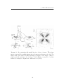
Dissertation Examination Committee:
Henric Krawczynski, Chair
James Buckley
Ramanath Cowsik
Mark Franklin
Martin Israel
Aaron Stump
OBSERVATIONS OF THE ACTIVE GALACIC NUCLEUS MARKARIAN 421
WITH THE FIRST TWO VERITAS ČERENKOV TELESCOPES
by
Scott Brandon Hughes
A dissertation presented to the
Graduate School of Arts and Sciences
of Washington University in
partial fulfillment of the
requirements for the degree
of Doctor of Philosophy
January 2007
Saint Louis, Missouri
Acknowledgements
I would like to thank my advisor, Dr. Henric Krawczynski, for all his help throughout my graduate school career. Dr. Jim Buckley and Dr. Martin Israel have also been
integral in my education, both in serving on my committee as well as being around to
provide fresh insight into my work. Thanks to the rest of my thesis defense committee
as well for their comments and opinions. I also thank Marty Olevitch, for providing both expert computer programming knowledge and sarcastic, spiteful retorts. I
thoroughly appreciate the help from Trevor Weekes and the entire VERITAS collaboration for not only creating a project that I have contributed so much to, but also
for their knowledge and assistance with problems too large for me to tackle alone.
I gratefully acknowledge the McDonnell Center for Space Sciences for a fellowship
that allowed me to jump-start my research immediately upon entering grad school.
Additionally, the staff at Washington University has been most helpful in this important process. Sarah Jordan, Julia Hamilton, Allison Verbeck, Jan Foster, Christine
Monteith, Paul Dowkontt, Ira Jung, and Richard Bose, among others, have all been
there at one time or another to help with administrative or technical problems that
crept up along the way.
ii
I cannot even begin to thank my fellow graduate students, past and present, for
their assistance, both intellectual and not so intellectual. In particular, to Jeremy
Perkins, Karl Kosack, Paul Rebillot, Lauren Scott, Randy Wolfmeyer, Mairin Hynes,
Allyson Gibson, Brian Rauch, Kuen “Vicky” Lee, Trey Garson, Kelly Lave, Frank
Gyngard, and honorary grad student Ellen Wurm, as well as many others I am not
able to list.
A special thanks goes out to Jason Rosch, who continually helped me to get out
and temporarily forget about my problems when the going got tough. Also, to Erica
Barnhill, who has been there since college whenever I needed someone to talk to and
is always able to cheer me up. In addition, to Morgann Reilly, who unintentionally
showed me that things could be much worse, and who was always up for a drink and
a movie to distract us both from our troubles at work.
Several others have also helped provide me with joy and amusement outside of
school during my stay in St. Louis. Most importantly, the ANTM crew—Danette
Wilson, Rose Martelli, Amber Specter, and Allyson Gibson (who does in fact deserve
to be mentioned again)—for that much-needed downward spiral into trashy TV. Anna
MacKay has also provided entertainment, though in much more than a “guilty pleasure” capacity. Finally, I must thank all my friends out in Phoenix. Most important
of these is Mike Drabick, who not only let me crash at his place when I needed to get
away, but without whom I would never have met any of the many other wonderful
people I have come to know in my visits out there.
iii
Contents
Acknowledgements
ii
List of Figures
viii
List of Tables
ix
Abstract
x
Copyright
xii
1 Summary of Thesis Work
1
2 Astrophysics of Blazars
2.1 Introduction to γ-ray Astrophysics . . . . . . . .
2.2 Instruments to Detect γ-rays . . . . . . . . . . . .
2.2.1 Space-based Instruments . . . . . . . . . .
Compton Gamma Ray Observatory . . . .
Swift . . . . . . . . . . . . . . . . . . . . .
GLAST . . . . . . . . . . . . . . . . . . .
2.2.2 Ground-based Instruments . . . . . . . . .
Imaging Atmospheric Čerenkov Telescopes
Čerenkov Solar Array Telescopes . . . . .
Particle Air Shower Arrays . . . . . . . . .
2.3 TeV γ-ray Sources . . . . . . . . . . . . . . . . .
2.4 Blazars . . . . . . . . . . . . . . . . . . . . . . . .
2.4.1 Spectral Energy Distributions . . . . . . .
2.4.2 Emission Models and Particle Acceleration
Synchrotron Self-Compton . . . . . . . . .
External Compton . . . . . . . . . . . . .
Hadronic Models . . . . . . . . . . . . . .
Particle Acceleration . . . . . . . . . . . .
2.4.3 Markarian 421 . . . . . . . . . . . . . . . .
iv
.
.
.
.
.
.
.
.
.
.
.
.
.
.
.
.
.
.
.
.
.
.
.
.
.
.
.
.
.
.
.
.
.
.
.
.
.
.
.
.
.
.
.
.
.
.
.
.
.
.
.
.
.
.
.
.
.
.
.
.
.
.
.
.
.
.
.
.
.
.
.
.
.
.
.
.
.
.
.
.
.
.
.
.
.
.
.
.
.
.
.
.
.
.
.
.
.
.
.
.
.
.
.
.
.
.
.
.
.
.
.
.
.
.
.
.
.
.
.
.
.
.
.
.
.
.
.
.
.
.
.
.
.
.
.
.
.
.
.
.
.
.
.
.
.
.
.
.
.
.
.
.
.
.
.
.
.
.
.
.
.
.
.
.
.
.
.
.
.
.
.
.
.
.
.
.
.
.
.
.
.
.
.
.
.
.
.
.
.
.
.
.
.
.
.
.
.
.
.
.
.
.
.
.
.
.
.
.
.
4
4
6
6
7
8
9
10
10
12
14
14
20
21
23
23
24
25
25
26
Contents
3 γ-ray Detection and VERITAS
3.1 γ-ray Propagation . . . . . . . . . . . . . . . . . . . . . . . . . . . . .
3.1.1 Propagation Through Space . . . . . . . . . . . . . . . . . . .
3.1.2 Air Showers in the Atmosphere . . . . . . . . . . . . . . . . .
γ-ray Induced Showers . . . . . . . . . . . . . . . . . . . . . .
Čerenkov Radiation . . . . . . . . . . . . . . . . . . . . . . . .
Cosmic Ray Induced Showers . . . . . . . . . . . . . . . . . .
3.2 Detection Using an Imaging Atmospheric Čerenkov Telescope (IACT)
3.2.1 Atmospheric Technique . . . . . . . . . . . . . . . . . . . . . .
3.2.2 Imaging Čerenkov Radiation . . . . . . . . . . . . . . . . . . .
3.3 VERITAS: Very Energetic Radiation Imaging Telescope Array System
3.3.1 Telescope Array . . . . . . . . . . . . . . . . . . . . . . . . . .
3.3.2 Camera . . . . . . . . . . . . . . . . . . . . . . . . . . . . . .
3.3.3 Trigger . . . . . . . . . . . . . . . . . . . . . . . . . . . . . . .
3.3.4 Data Acquisition . . . . . . . . . . . . . . . . . . . . . . . . .
28
28
29
29
30
31
33
33
33
35
37
37
39
42
43
4 Mrk 421 Data Analysis
4.1 Event Reconstruction . . . . . . . . . . . . . . . . .
4.1.1 Hillas Parameterization . . . . . . . . . . . .
4.1.2 Stereo Reconstruction . . . . . . . . . . . .
4.1.3 Analysis Tools . . . . . . . . . . . . . . . . .
4.2 Data Cuts and Significances . . . . . . . . . . . . .
4.3 Spectral Reconstruction . . . . . . . . . . . . . . .
4.4 Mrk 421 Data from April–May 2006 . . . . . . . . .
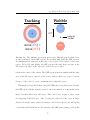
4.4.1 Observation Modes . . . . . . . . . . . . . .
ON–OFF Pairs . . . . . . . . . . . . . . . .
Tracking Runs . . . . . . . . . . . . . . . . .
Wobble Runs . . . . . . . . . . . . . . . . .
4.4.2 Final Data Set . . . . . . . . . . . . . . . .
4.5 Comparison of Experimental and Monte Carlo Data
4.6 First Stereo Results from VERITAS . . . . . . . . .
4.6.1 Cutting on θ2 . . . . . . . . . . . . . . . . .
4.6.2 Cutting on Mean Scaled Width . . . . . . .
4.6.3 Mrk 421 Light Curve . . . . . . . . . . . . .
4.6.4 Energy Spectrum . . . . . . . . . . . . . . .
.
.
.
.
.
.
.
.
.
.
.
.
.
.
.
.
.
.
44
44
45
47
50
51
52
53
53
54
54
56
56
58
64
65
67
68
70
. . . . .
. . . . .
. . . . .
. . . . .
. . . . .
(DCF) .
71
71
72
74
76
81
84
5 SSC Modeling of Blazar Emission
5.1 Rationale . . . . . . . . . . . . . . . .
5.2 Measurement of the Jet Magnetic Field
5.3 Synchrotron Self-Compton Simulations
5.4 Generating Data Sets . . . . . . . . . .
5.5 Analysis Procedure . . . . . . . . . . .
5.6 Measuring Time Lags with the Discrete
v
.
.
.
.
.
.
.
.
.
.
.
.
.
.
.
.
.
.
.
.
.
.
.
.
.
.
.
.
.
.
.
.
.
.
.
.
.
.
.
.
.
.
.
.
.
.
.
.
.
.
.
.
.
.
.
.
.
.
.
.
.
.
.
.
.
.
.
.
.
.
.
.
.
.
.
.
.
.
.
.
.
.
.
.
.
.
.
.
.
.
. . . . . . . . . . . .
. . . . . . . . . . . .
. . . . . . . . . . . .
. . . . . . . . . . . .
. . . . . . . . . . . .
Correlation Function
.
.
.
.
.
.
.
.
.
.
.
.
.
.
.
.
.
.
.
.
.
.
.
.
.
.
.
.
.
.
.
.
.
.
.
.
.
.
.
.
.
.
.
.
.
.
.
.
.
.
.
.
.
.
.
.
.
.
.
.
.
.
.
.
.
.
.
.
.
.
.
.
Contents
5.7
Comparing of DCF Time Lags to Expected Results . . . . . . . . . .
91
6 Discussion
6.1 Summary of Thesis Results . . . . . . . . . . . . . . . . . . . . . . .
6.2 VERITAS Performance . . . . . . . . . . . . . . . . . . . . . . . . . .
6.3 The Future of γ-ray Astrophysics . . . . . . . . . . . . . . . . . . . .
94
94
95
97
A X-ray Data Analysis of 1ES 1959+650 and Mrk 421
99
A.1 Multiwavelength Campaign Overview . . . . . . . . . . . . . . . . . . 99
A.2 RXTE Data . . . . . . . . . . . . . . . . . . . . . . . . . . . . . . . . 100
A.3 “Orphan” Flares . . . . . . . . . . . . . . . . . . . . . . . . . . . . . 102
B Daily VERITAS Data Quality Monitoring
B.1 Motivation and Procedure . . . . . . . . . . . . . . . . . . . . . . . .
B.2 Analysis and Results . . . . . . . . . . . . . . . . . . . . . . . . . . .
B.3 The dt Bump . . . . . . . . . . . . . . . . . . . . . . . . . . . . . . .
105
105
106
110
C VAC: VERITAS Array Control GUI
C.1 Starting VAC . . . . . . . . . . . . . . .
C.1.1 Normal Operation . . . . . . . .
C.1.2 Debugging Systems . . . . . . . .
C.2 Using the VAC . . . . . . . . . . . . . .
C.2.1 Main Window . . . . . . . . . . .
System Status . . . . . . . . . . .
Run Management . . . . . . . . .
Run Info for Current Active Run
L2/L3 Rate Plot . . . . . . . . .
C.2.2 Observer Menu . . . . . . . . . .
C.2.3 Test Runs Menu . . . . . . . . .
C.2.4 Subsystems Menu . . . . . . . . .
L3 Subsystem . . . . . . . . . . .
Harvester Subsystem . . . . . . .
Event Builder Subsystem . . . . .
L2 Subsystem . . . . . . . . . . .
L1 Subsystem . . . . . . . . . . .
Database Subsystem . . . . . . .
Charge Injection (QI) Subsystem
Custom Night . . . . . . . . . . .
C.2.5 Settings Menu . . . . . . . . . . .
Put CFD Settings . . . . . . . . .
CFD Settings . . . . . . . . . . .
FADC Settings . . . . . . . . . .
112
113
113
114
115
115
115
118
123
124
125
129
130
130
132
133
135
136
136
139
139
141
141
142
142
vi
.
.
.
.
.
.
.
.
.
.
.
.
.
.
.
.
.
.
.
.
.
.
.
.
.
.
.
.
.
.
.
.
.
.
.
.
.
.
.
.
.
.
.
.
.
.
.
.
.
.
.
.
.
.
.
.
.
.
.
.
.
.
.
.
.
.
.
.
.
.
.
.
.
.
.
.
.
.
.
.
.
.
.
.
.
.
.
.
.
.
.
.
.
.
.
.
.
.
.
.
.
.
.
.
.
.
.
.
.
.
.
.
.
.
.
.
.
.
.
.
.
.
.
.
.
.
.
.
.
.
.
.
.
.
.
.
.
.
.
.
.
.
.
.
.
.
.
.
.
.
.
.
.
.
.
.
.
.
.
.
.
.
.
.
.
.
.
.
.
.
.
.
.
.
.
.
.
.
.
.
.
.
.
.
.
.
.
.
.
.
.
.
.
.
.
.
.
.
.
.
.
.
.
.
.
.
.
.
.
.
.
.
.
.
.
.
.
.
.
.
.
.
.
.
.
.
.
.
.
.
.
.
.
.
.
.
.
.
.
.
.
.
.
.
.
.
.
.
.
.
.
.
.
.
.
.
.
.
.
.
.
.
.
.
.
.
.
.
.
.
.
.
.
.
.
.
.
.
.
.
.
.
.
.
.
.
.
.
.
.
.
.
.
.
.
.
.
.
.
.
.
.
.
.
.
.
.
.
.
.
.
.
.
.
.
.
.
.
.
.
.
.
.
.
.
.
.
.
.
.
.
.
.
.
.
.
.
.
.
.
.
.
.
.
.
.
.
.
.
.
.
.
.
.
.
.
.
.
.
.
.
.
.
.
.
.
.
.
.
.
.
.
.
.
.
.
.
.
.
.
.
.
.
.
List of Figures
2.1 The Compton Gamma Ray Observatory (CGRO) . . .
2.2 The Gamma-ray Large Area Space Telescope (GLAST)
2.3 The Whipple 10 m Telescope . . . . . . . . . . . . . . .
2.4 The H.E.S.S. Telescopes . . . . . . . . . . . . . . . . .
2.5 Sky Map of γ-ray Sources . . . . . . . . . . . . . . . .
2.6 The Crab Nebula . . . . . . . . . . . . . . . . . . . . .
2.7 Schematic of an Active Galactic Nucleus . . . . . . . .
2.8 Sample Spectral Energy Distribution . . . . . . . . . .
2.9 X-ray Light Curve of Mrk 421 with Flares . . . . . . .
.
.
.
.
.
.
.
.
.
.
.
.
.
.
.
.
.
.
.
.
.
.
.
.
.
.
.
.
.
.
.
.
.
.
.
.
.
.
.
.
.
.
.
.
.
.
.
.
.
.
.
.
.
.
.
.
.
.
.
.
.
.
.
.
.
.
.
.
.
.
.
.
7
9
11
13
15
18
20
22
27
3.1
3.2
3.3
3.4
3.5
3.6
3.7
3.8
Electromagnetic Cascading Air Shower . . . . . . . .
Čerenkov Radiation . . . . . . . . . . . . . . . . . . .
Charged Particle Polarizing the Surrounding Medium
Cosmic Ray Air Showers . . . . . . . . . . . . . . . .
Cosmic Ray vs. γ-ray Air Showers . . . . . . . . . . .
Layout of the Four VERITAS Telescopes . . . . . . .
A 12 m VERITAS Telescope . . . . . . . . . . . . . .
PMT Camera . . . . . . . . . . . . . . . . . . . . . .
.
.
.
.
.
.
.
.
.
.
.
.
.
.
.
.
.
.
.
.
.
.
.
.
.
.
.
.
.
.
.
.
.
.
.
.
.
.
.
.
.
.
.
.
.
.
.
.
.
.
.
.
.
.
.
.
.
.
.
.
.
.
.
.
30
31
32
34
36
38
40
41
4.1
4.2
4.3
4.4
4.5
4.6
4.7
4.8
4.9
4.10
4.11
4.12
4.13
4.14
4.15
Hillas Parameters . . . . . . . . . . . . . . . . . . .
Images of Sky Showers . . . . . . . . . . . . . . . .
Stereo Shower Reconstruction . . . . . . . . . . . .
OFF regions . . . . . . . . . . . . . . . . . . . . . .
Comparing Monte Carlo Simulations to Data . . . .
Energy Threshold of Monte Carlo Simulations . . .
Angular Resolution of Monte Carlo Simulations . .
Core Resolution of Monte Carlo Simulations . . . .
True vs. Reconstructed Energy for the Monte Carlo
Plots of θ2 . . . . . . . . . . . . . . . . . . . . . . .
Q-factor for θ2 . . . . . . . . . . . . . . . . . . . . .
Plot of M SCW . . . . . . . . . . . . . . . . . . . .
Q-factor for M SCW . . . . . . . . . . . . . . . . .
Mrk 421 Light Curve . . . . . . . . . . . . . . . . .
Energy Spectrum of Mrk 421 . . . . . . . . . . . .
. . . . . . .
. . . . . . .
. . . . . . .
. . . . . . .
. . . . . . .
. . . . . . .
. . . . . . .
. . . . . . .
Simulations
. . . . . . .
. . . . . . .
. . . . . . .
. . . . . . .
. . . . . . .
. . . . . . .
.
.
.
.
.
.
.
.
.
.
.
.
.
.
.
.
.
.
.
.
.
.
.
.
.
.
.
.
.
.
.
.
.
.
.
.
.
.
.
.
.
.
.
.
.
46
48
49
55
60
61
62
63
64
66
67
68
68
69
70
vii
.
.
.
.
.
.
.
.
List of Figures
5.1
5.2
5.3
5.4
5.5
5.6
5.7
5.8
Sample Input of Simulated Flares . .
SEDs of Simulated Data Sets . . . .
Light Curves of Simulated Data Sets
DCF from Simulated Data . . . . . .
Actual vs. Calculated Lag Times . .
Actual vs. Calculated B Fields . . .
DCF over Different Energy Ranges .
DCF for Flares of Different Durations
.
.
.
.
.
.
.
.
.
.
.
.
.
.
.
.
.
.
.
.
.
.
.
.
.
.
.
.
.
.
.
.
.
.
.
.
.
.
.
.
.
.
.
.
.
.
.
.
.
.
.
.
.
.
.
.
.
.
.
.
.
.
.
.
.
.
.
.
.
.
.
.
.
.
.
.
.
.
.
.
.
.
.
.
.
.
.
.
.
.
.
.
.
.
.
.
.
.
.
.
.
.
.
.
.
.
.
.
.
.
.
.
.
.
.
.
.
.
.
.
.
.
.
.
.
.
.
.
.
.
.
.
.
.
.
.
.
.
.
.
.
.
.
.
77
79
80
85
87
88
89
90
6.1
Observatory Sensitivity . . . . . . . . . . . . . . . . . . . . . . . . . .
96
A.1 “Orphan” Flare of 1ES 1959+650 . . . . . . . . . . . . . . . . . . . . 103
B.1 Representative Good DDQM Plots . . . . . . . . . . . . . . . . . . . 108
B.2 Representative Poor DDQM Plots . . . . . . . . . . . . . . . . . . . . 109
B.3 The dt Bump . . . . . . . . . . . . . . . . . . . . . . . . . . . . . . . 111
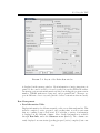
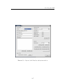
C.1 Main VAC Window . . . . . . . .
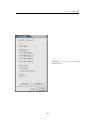
C.2 Define Run Window . . . . . . .
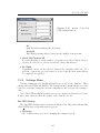
C.3 Run Info Window . . . . . . . . .
C.4 L3 Subsystem Window . . . . . .
C.5 Harvester Subsystem Window . .
C.6 Event Builder Subsystem Window
C.7 L2 Subsystem Window . . . . . .
C.8 Database Subsystem Window . .
C.9 Custom Night Window . . . . . .
C.10 Put CFD Settings Window . . . .
viii
.
.
.
.
.
.
.
.
.
.
.
.
.
.
.
.
.
.
.
.
.
.
.
.
.
.
.
.
.
.
.
.
.
.
.
.
.
.
.
.
.
.
.
.
.
.
.
.
.
.
.
.
.
.
.
.
.
.
.
.
.
.
.
.
.
.
.
.
.
.
.
.
.
.
.
.
.
.
.
.
.
.
.
.
.
.
.
.
.
.
.
.
.
.
.
.
.
.
.
.
.
.
.
.
.
.
.
.
.
.
.
.
.
.
.
.
.
.
.
.
.
.
.
.
.
.
.
.
.
.
.
.
.
.
.
.
.
.
.
.
.
.
.
.
.
.
.
.
.
.
.
.
.
.
.
.
.
.
.
.
.
.
.
.
.
.
.
.
.
.
.
.
.
.
.
.
.
.
.
.
.
.
.
.
.
.
.
.
.
.
.
.
.
.
.
.
.
.
.
.
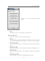
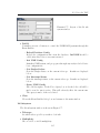
116
118
128
130
132
134
135
137
140
141
List of Tables
2.1
2.2
γ-ray Nomenclature . . . . . . . . . . . . . . . . . . . . . . . . . . . .
TeV γ-ray Sources . . . . . . . . . . . . . . . . . . . . . . . . . . . .
5
16
4.1
4.2
Final Mrk 421 Data Set . . . . . . . . . . . . . . . . . . . . . . . . .
Monte Carlo Angular Resolution . . . . . . . . . . . . . . . . . . . . .
57
62
5.1
5.2
5.3
Parameters for Simulated Data Files . . . . . . . . . . . . . . . . . .
Calculated and Observed Time Lags . . . . . . . . . . . . . . . . . .
Observed and Calculated B fields . . . . . . . . . . . . . . . . . . . .
78
86
87
ix
Abstract
This thesis describes two projects, the first of which is the analysis of data from the
VERITAS (Very Energetic Radiation Imaging Telescope Array System) experiment.
VERITAS, an array of ground-based γ-ray telescopes in southern Arizona, USA,
has been taking data in hardware stereo mode since March, 2006. The April–May
2006 dark run provided a large set of data from two telescopes on the known blazar
Markarian (Mrk) 421. An initial analysis of the 14.3 hours of stereo data produced
a light curve and confirmed a detection on the 39 sigma level with a γ-ray rate of
2.91±0.07γ min−1 , reduced from an inferred value of 8.83±0.21γ min−1 before analysis
cuts. The analysis shows the two-telescope array’s energy threshold to be 165 GeV
before cuts and 220 GeV after cuts, with an angular resolution of 0.16◦ . These data
were also used to extract an energy spectrum for Mrk 421. This initial analysis allows
a test of the performance of the two-telescope array and gives an idea of the data
that will come from the full system. The remaining two VERITAS telescopes will
be brought online by January, 2007. As a second project, computer simulations were
used to model Synchrotron Self-Compton (SSC) emission from blazars that will be
relevant for future multiwavelength campaigns. The Discrete Correlation Function
x
List of Tables
(DCF) was used to calculate the source’s magnetic field based on the time lag between
emission in different X-ray energy bands. This method, used by different authors in
the literature, was shown to overestimate the magnetic field by as much as a factor
of six. Understanding the behavior of properties such as this will allow the breaking
of model degeneracies and give insight into the physical processes involved in particle
acceleration of blazars.
xi
This work is licensed under the Creative Commons
Attribution-NonCommercial-ShareAlike2.5 License.
To view a copy of this license, visit
http://creativecommons.org/licenses/by-nc-sa/2.5/
or send a letter to
Creative Commons,
543 Howard Street, 5th Floor,
San Francisco, California, 94105, USA.
Chapter 1
Summary of Thesis Work
For this thesis, I looked at the first true stereo data taken with two of the planned
four VERITAS
1
γ-ray telescopes. The April–May 2006 dark run provided a large
amount of data on the known blazar Markarian (Mrk) 421. These data were used to
verify that the VERITAS system is performing as expected. They were also used to
determine some loose data cuts to use in the future. Also, VERITAS’s first energy
spectrum of this source was derived. The results of this initial data analysis help us
understand what type of data we may get once the entire telescope system is up and
running. It will also allow us to tweak our simulations so they more accurately model
the telescopes’ behavior.
Operating the VERITAS experiment requires software. I worked to design and
1
VERITAS (Very Energetic Radiation Imaging Telescope Array System) is supported by grants
from the U. S. Department of Energy, the U. S. National Science Foundation, the Smithsonian
Institution, by NSERC in Canada, by Science Foundation Ireland, and by PPARC in the U. K. It is
being built through a collaboration of nine primary universities and the Smithsonian Astrophysical
Observatory, as well as several other contributing institutions. http://veritas.sao.arizona.edu
1
write the entire graphical interface to arrayctl, the array control program written
by Marty Olevitch. arrayctl is responsible for coordinating and overseeing all data
taking processes for the entire array. The graphical interface, called VAC (VERITAS
Array Control), can oversee many aspects of daily observation. It is used to manage
data taking, and also displays feedback and data plots from the various subsystems
to ensure system and data integrity. VAC has become the most important and most
depended upon piece of software for VERITAS telescope operation.
Observations have to be complemented with theoretical modeling to reveal the
physical processes that produce the observed emission. I worked with a Synchrotron
Self-Compton (SSC) simulation code to explore time lags in the light curves measured
in different observational bands. Using the Discrete Correlation Function (DCF), one
can determine this lag. From that, it is a common approach to calculate the magnetic
field of the source. Various parameters were altered and different scenarios tried in
order to test the accuracy of this method. Understanding the behavior of properties
such as this will allow the breaking of model degeneracies and give insight into the
physical processes involved in particle acceleration of blazars.
The text of this thesis is organized as follows. An introduction to γ-ray astrophysics is covered in Chapter 2, focusing on blazars and their observation. A description of how γ-rays are detected on Earth, and the VERITAS telescopes in particular,
are covered in Chapter 3. Following are details on the analysis and results from the
first VERITAS stereo data in Chapter 4. A complete description of the SSC simulations used to test the DCF as a tool for measuring the magnetic field of sources is
2
given in Chapter 5, concluding with a discussion of all results, as well as the future
of γ-ray astrophysics and VERITAS, in Chapter 6.
The Appendices describe various other studies I have performed during the course
of this thesis. A brief overview of the X-ray analyses of Mrk 421 and 1ES 1959+650
are covered in Appendix A. A summary of daily data quality monitoring (DDQM)
for the VERITAS telescopes is given in Appendix B. Finally, a description and User’s
Manual for the graphical interface VAC is presented in Appendix C.
3
Chapter 2
Astrophysics of Blazars
2.1
Introduction to γ-ray Astrophysics
At the high-energy end of the electromagnetic spectrum lie what are called “γrays”. Photons in this range have the shortest wavelengths, and energies from around
500 keV to through TeV and even higher. The energy range covered by γ-rays is more
than that of the rest of the electromagnetic spectrum combined (Weekes, 2003). In
order to talk about γ-rays, it is appropriate to divide the energy range into smaller
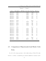
sections of similar behavior and detection techniques. Table 2.1 lists the common
nomenclature and their corresponding energy ranges.
In order to produce γ-rays, charged particles (electrons, positrons, protons, or
other nuclei) must be accelerated to extremely high energies. The particles then emit
radiation, which travels through space as γ-rays. There are several relevant emission
mechanisms. Synchrotron radiation is emitted when a relativistic charged particle
4
2.1 Introduction to γ-ray Astrophysics
Table 2.1: The common divisions within the span of γ-ray energies, including
common descriptive names.
Common Name
Low (LE)
Medium (ME)
High (HE)
Very High (VHE)
Ultrahigh (UHE)
Extremely High (EHE)
Energy Range
500 keV − 10 MeV
10 MeV − 30 MeV
30 MeV − 30 GeV
30 GeV − 30 TeV
30 TeV − 30 PeV
30 PeV and up
spirals around a magnetic field line. To generate TeV photons by this mechanism,
either rather strong magnetic fields ( 1 G) or extremely high-energy electrons or
protons are required. Another process is Bremsstrahlung, which occurs when an
electron is decelerated by the electromagnetic field of a charged particle or particles.
The “braking radiation” produced is a result of the energy loss by the electron, and
can be quite substantial. Perhaps the most important process is inverse Compton
scattering. When a low-energy photon collides with an energetic electron, it can
be scattered to much higher energies. All these processes are described in detail in
Section 2.4.2.
γ-rays can be detected through their interaction with matter. Different energy
ranges lend themselves to different dominant interaction processes. For the lowestenergy γ-rays, photoelectric absorption is the dominant process. A γ-ray can eject
an electron from a tightly bound atom, which also emits an X-ray as the resulting
hole in the atom is filled by an electron from a higher orbit. Both the ejected electron
and X-ray can be used to detect the original γ-ray. Mid-range γ-rays prefer Compton
5
2.2 Instruments to Detect γ-rays
scattering. Here, a γ-ray collides with a loosely bound electron, giving up some of its
energy. Multiple collisions can occur for the same incident γ-ray. For higher-energy
photons, the dominant process is pair production. If the γ-ray photon has energy
Eγ > 2m0 c2 = 1.022 MeV
(2.1)
where m0 is the rest mass of the electron, it can convert to an electron-positron pair
in the presence of an atomic nucleus, required for momentum conservation.
2.2
Instruments to Detect γ-rays
Being uncharged and therefore unaffected by magnetic fields permeating the universe, γ-rays are very directional and arrive at Earth from distinct points in the sky.
The Earth’s atmosphere is opaque to γ-rays, so the only way to see them directly
is from space. However, indirect techniques have been developed to observe γ-ray
sources from the ground as well (see Sect. 2.2.2).
2.2.1
Space-based Instruments
Early balloon experiments detecting cosmic rays suggested that moving beyond
the Earth’s atmosphere might be advantageous to finding even higher-energy γ-rays.
Despite its small collection area and poor angular resolution, the Explorer XI satellite,
launched in 1965, was able to prove the existence of γ-rays originating outside the
Earth’s atmosphere (Clark et al., 1968). The practice of using balloons for flying
spark chambers to detect γ-rays was effectively ended in 1972 with the launch of
6
2.2 Instruments to Detect γ-rays
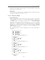
Figure 2.1: A collection of several instruments including EGRET (center) and
BATSE (eight detectors, one on each corner of the spacecraft), the Compton Gamma
Ray Observatory was highly successful in observing a wide range of γ-ray phenomena.
Figure from http://cossc.gsfc.nasa.gov.
NASA’s SAS-2. The European Space Agency’s COS-B was launched soon after in
1975. By helping map the γ-ray sky in detail, both these telescopes established γ-ray
astronomy as a new and exciting field worthy of further study.
Compton Gamma Ray Observatory
The most successful space-based γ-ray telescope to date has been the Compton Gamma Ray Observatory (CGRO; Gehrels et al., 1993), shown in Figure 2.1.
Launched in 1991, it remained in orbit for over nine years. It was built to observe
γ-rays over the energy range of 15 keV − 30 GeV with several different instruments.
7
2.2 Instruments to Detect γ-rays
Each of the instruments onboard the CGRO was designed for a specific purpose.
The Burst and Transient Source Experiment (BATSE) was able to detect γ-ray bursts
(GRBs) on microsecond time scales in the 20keV−1.9MeV energy range. The Compton Telescope (COMPTEL) provided the first sky survey in the 1 − 30 MeV band.
The Oriented Scintillation Spectroscopy Experiment (OSSE) performed spectral observations in the 0.05 − 10 MeV energy range.
The final instrument was EGRET, the Energetic Gamma Ray Experiment Telescope. Operating at the highest energies of any of CGRO’s components (10 MeV −
30 GeV), EGRET was able to detect over 250 new γ-ray sources in its lifetime, 66 of
which were blazars (Thompson et al., 1995; Hartman et al., 1999). The detector itself
was massive. The amount of material needed to stop the high energy photons had a
mass of 1900 kg and was approximately the size of a compact car, yet had an effective
collection area of only 1600 cm2 (Fichtel et al., 1993). More recent experiments are
able to accomplish more with a lighter detector.
Swift
With the retirement of the CGRO, we were left without a reliable method to detect
and report GRBs. Then, in 2004, NASA launched Swift (Burrows et al., 2003), which
contained the Burst Alert Telescope (BAT) with five times the sensitivity of BATSE.
The satellite is also made up of telescopes for monitoring these bursts in X-rays, UV,
and optical bands. This multiwavelength ability helps Swift to detect GRB positions
within a few arc seconds.
8
2.2 Instruments to Detect γ-rays
Figure 2.2: Set to launch in
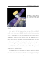
2007, GLAST represents the future of space-based γ-ray astronomy.
GLAST
Set to launch in 2007, the Gamma-ray Large Area Space Telescope (GLAST;
see Fig. 2.2) is the successor of EGRET, and will be able to detect sources from
20 MeV − 300 GeV (Ritz et al., 2005). Its sensitivity will be almost 10 times that of
EGRET and it will have about twice the field of view. Like EGRET, GLAST is a
pair production telescope. The primary γ-ray interacts with the detector and creates
an electron-positron pair. The two charged particles are then tracked through the
detector volume. The tracks point back towards the incident direction of the primary
γ-ray. GLAST will also have a basic ability to detect GRBs. The experiment is
described in more detail in Section 6.3.
Though many technological advancements are being made, limits to the physical
size of these space-borne detectors, as well as the sources’ steep spectra at higher
9
2.2 Instruments to Detect γ-rays
energies, prevent their being used to detect γ-rays at energies > 300 GeV. To probe
higher energy γ-rays, it is necessary to use ground-based detectors.
2.2.2
Ground-based Instruments
The Earth’s atmosphere is opaque to γ-rays. However, it is still possible to detect the results of their interactions with the Earth’s atmosphere. This process is
described more in Chapter 3. Ground-based techniques have proven highly effective
in observing and discovering new sources of γ-rays. Čerenkov telescopes in particular
have discovered TeV emission from seven blazars, five of which were not detected by
EGRET (Horan and Weekes, 2004; Aharonian et al., 2005a).
Imaging Atmospheric Čerenkov Telescopes
Taking over where space-based detectors leave off, Imaging Atmospheric Čerenkov
Telescopes (IACTs) operate in the 30 GeV − 30 TeV range. First proposed by Weekes
and Turver (1977), this technique is based on detecting flashes of Čerenkov light
resulting from interactions as the primary γ-ray passes through Earth’s atmosphere.
It is discussed further in Section 3.2.
Stand-alone IACTs have been operating for years with optical reflectors ranging
from 3 − 17 m in diameter. Examples of early and present telescopes include CAT
in France (Barrau et al., 1998), the Whipple 10 m in Arizona, USA (Cawley et al.,
1990), and MAGIC in the Canary Islands (Lorenz and Martinez, 2005). An example
of this type of telescope can be seen in Figure 2.3.
10
2.2 Instruments to Detect γ-rays
Figure 2.3: Located on Mt. Hopkins in southern Arizona, USA, the Whipple 10 m
telescope is an example of an Imaging Atmospheric Čerenkov Telescope.
11
2.2 Instruments to Detect γ-rays
The current trend in IACTs is to use an array of telescopes all looking at the same
source and requiring multiple telescope coincidences for the array to trigger. This
method, first pioneered by HEGRA (Pühlhofer et al., 2003), has several advantages
over single telescopes. Arrays of IACTs provide a large effective area (> 100 m2 ),
excellent suppression of cosmic ray initiated air showers and local muons, lower energy
threshold, improved angular resolution, and better flux sensitivity, as well as better
energy resolution compared to their single-telescope counterparts.
Recently, most new discoveries have come from the H.E.S.S. (High Energy Stereoscopic System) array in Namibia, Africa (Aharonian et al., 2005d). Shown in Figure 2.4, H.E.S.S. consists of four 12 m telescopes and has been able to detect an
astounding number (∼ 30) of new sources since coming online in 2003.
Other arrays of IACTs are currently being built around the world. VERITAS,
described in Section 3.3, is nearing completion in southern Arizona, USA. The MAGIC
Collaboration is also building a second telescope at their current site to create the
two-telescope array MAGIC II.
Čerenkov Solar Array Telescopes
Čerenkov light can also be collected by the large mirrors of solar detectors. Originally proposed by Danaher et al. (1982), several groups such as STACEE (Gingrich
et al., 2005) and CELESTE (Smith et al., 2006) have since implemented the technique. Čerenkov radiation is reflected off the large solar mirrors and focused onto
photomultiplier tubes (PMTs). The shower direction is inferred from the arrival
12
2.2 Instruments to Detect γ-rays
Figure 2.4: The four H.E.S.S. telescopes, located in Namibia, Africa, are an example
of an array of IACTs.
13
2.3 TeV γ-ray Sources
times of the light from each of the solar panels. Due to their large collection area,
these telescopes have lower operating energies than single IACTs.
Particle Air Shower Arrays
Though originally built to study the properties of cosmic rays (Ter Haar, 1950),
particle air shower arrays can be used to study γ-rays in the TeV–PeV energy regime.
The most successful such detector is MILAGRO, located in New Mexico, USA, which
operates at ∼ 1 TeV (Dingus et al., 2000). Inside a large pool of water are 723
PMTs used to detect residual particles from air showers. However, this type of
detector achieves a limited separation between charged cosmic rays and γ-rays (see,
e.g., Catanese and Weekes, 1999).
2.3
TeV γ-ray Sources
Just as there is not one mechanism to detect the whole range of γ-rays, there
are also many types of sources from which these rays can originate. The number
of sources detected has sharply increased in recent years as well, due mostly to the
H.E.S.S. telescopes in the Southern Hemisphere. A similar increase in new sources in
the Northern Hemisphere should happen shortly, when VERITAS comes fully online.
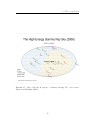
Figure 2.5 shows a map of the sky in galactic coordinates, with all known TeV sources
labeled. These sources are also listed in Table 2.2
14
2.3 TeV γ-ray Sources
Figure 2.5: Map of the sky in galactic coordinates showing TeV γ-ray sources.
Figure from Hermann (2006).
15
2.3 TeV γ-ray Sources
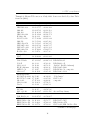
Table 2.2: Known TeV sources as of July, 2006. Sources are divided by class. Table
from Cui (2006).
Name
Blazar:
1ES 1101−232
Mrk 421
Mrk 180
1ES 1218+304
H 1426+428
PG 1553+113
Mrk 501
1ES 1959+650
PKS 2005−489
PKS 2155−304
1ES 2344+514
H 2356−309
Radio Galaxy:
M 87
Plerion:
Crab Nebula
Vela X
G313.3+0.1
K3/Kookaburra
MSH 15−52
G18.0−0.7
Shell-Type SNR:
RX J0852.0−4622
RX J1713.7−3946
G0.9+0.1
G12.82−0.02
Cas A
Pulsar:
LS 5039
LS I +61 303
X-ray Binary:
PSR B1259−63
Unidentified:
HESS J1616−508
HESS J1632−478
HESS J1634−472
RA (2000)
Dec (2000)
11
11
11
12
14
15
16
19
20
21
23
23
−23
+38
+70
+30
+42
+11
+39
+65
−48
−30
+51
−30
03
04
36
21
28
55
53
59
09
58
47
59
37.57
27.31
26.41
21.94
32.6
43.04
52.22
59.85
25.39
52.07
04.92
07.8
29
12
09
10
40
11
45
08
49
13
42
37
Notes
30.2
31.8
27.3
37.1
29
24.4
36.6
54.7
53.7
32.1
17.9
38
12 30 49.42 +12 23 28.0
05
08
14
14
15
18
34
33
18
20
14
26
31.97
32
04
09
07
03.0
+22
−45
−60
−60
−59
−13
00
43
58
48
09
45
52.1
42
31
36
27
44
PSR B0532+21
PSR B0833−45
“Rabbit” (R2/Kookaburra)
PSR J1420−6048
PSR B1509−58; composite
PSR J1826−1334
08
17
17
18
23
52
13
47
13
23
00
00
23.2
36.6
24
−46
−39
−28
−17
+58
20
45
09
50
48
00
00
06
35
54
“Vela Junior”
G347.3−0.5
composite
18 26 15
−14 50 53.6
02 40 31.67 +61 13 45.6 also an X-ray binary
13 02 47.65 −63 50 08.7
16 16 23.6
16 32 08.6
16 34 57.2
−50 53 57
−47 49 24
−47 16 02
16
PSR J1617−5055
IGR J16320−4751
G337.2+0.1/IGR J16358−4726
Continued on next page. . .
2.3 TeV γ-ray Sources
Table 2.2 – Continued
Name
HESS J1640−465
HESS J1713−381
HESS J1745−290
HESS J1804−216
HESS J1834−087
HESS J1837−069
HESS J1303−631
HESS J1614−518
HESS J1702−420
HESS J1708−410
HESS J1745−303
TeV J2032+4131
RA (2000)
16 40 44.2
17 13 58.0
17 45 41.3
18 04 31.6
18 34 46.5
18 37 37.4
13 03 00.4
16 14 19.0
17 02 44.6
17 08 14.3
17 45 02.2
20 31 57
Dec (2000)
−46 31 44
−38 11 43
−29 00 22
−21 42 03
−08 45 52
−06 56 42
−63 11 55
−51 49 07
−42 04 22
−41 04 57
−30 22 14
+41 29 56.8
Notes
G338.3−0.0/3EG J1639−4702
G348.7+0.3
G359.95−0.04/SgrA East/SgrA*
G8.7−0.1/PSR J1803−2137
G23.3−0.3
G25.5+0.0/AX J1838−0655
3EG J1744−3011
There are several classes of TeV γ-ray sources, the first of which are supernova
remnants (SNRs). The expanding shell of gas from a supernova explosion consists of
stellar material altered by the explosion as well as parts of the interstellar medium
swept up during expansion. In shell-type SNR, like RX J1713.7−3946, the emission
appears to come from an outer shell with no apparent central power source. Plerions,
like the Crab Nebula, are thought to be powered by a central pulsar.
The Crab Nebula is a particularly interesting TeV source for many reasons. The
supernova that created it exploded in 1054 AD and was observed by Chinese astronomers. It left behind a bright spot in the sky visible in daylight for weeks after.
The Crab was the first confirmed TeV γ-ray source, discovered by Weekes et al.
(1989). It has since become known for its strong, steady signal. Today it is used as
the “standard candle” by which all γ-ray observations are measured. A view of the
Crab with the Hubble Space Telescope can be seen in Figure 2.6.
17
2.3 TeV γ-ray Sources
Figure 2.6: The Crab Nebula as seen by the Hubble Space Telescope. The image
is 6.5 arcmin across, corresponding to 3.4 pc at a distance of ∼ 2 kpc.
18
2.3 TeV γ-ray Sources
Another known source class for TeV emission is X-ray binaries (XRBs). Though
mainly emitting X-rays, they also have been known to produce sporadic γ-ray emission
from the gas accreting onto the compact star in the binary pair. So far only two XRB
sources of γ-rays have been detected, PSR B1259−63 (Aharonian et al., 2005b) and
LS I +61303, also a pulsar (Albert et al., 2006).
The largest group of sources from which γ-rays have been detected are Active
Galactic Nuclei (AGN). These galaxies contain a very compact core emitting an extremely disproportionate amount of energy compared to the rest of the galaxy. This
central engine is thought to be a supermassive black hole surrounded by an accretion
disk (see Fig. 2.7). The disk is surrounded by fast-moving clouds of dust that, in
some cases, obscure the central engine from view, though these clouds can produce
Doppler-broadened emission lines. Farther from the nucleus, in the direction perpendicular to the plane of the accretion disk, narrow emission lines are produced through
scattering of the slower (less Doppler broadening) and less dense clouds surrounding
the galaxy. In some AGN, jets of highly relativistic particles are ejected out the poles
of the spinning central nucleus. These jets contain large magnetic fields capable of
producing synchrotron radiation up to X-ray wavelengths. Inverse Compton scattering from the jets’ relativistic electrons can also produce γ-rays. All but one AGN
detected in TeV γ-rays are part of the subclass known as blazars, discussed further
in Section 2.4. The one exception is the nearby radio galaxy M87 (Aharonian et al.,
2003, 2006). Its jet is believed to be at an angle of ∼ 30◦ to the line of sight.
19
2.4 Blazars
Figure 2.7: Model for the structure of an AGN, consisting of a
dense, central emitting region and
including jets of relativistic particles. The radius of the central
black hole is ∼ 10−4 pc, while the
jets can extend from 10−2 pc to
kpc or even Mpc from the black
hole. When the jets point towards
the Earth, the source is known as
a blazar. Figure from Holt et al.
(1992).
2.4
Blazars
Blazars are a subclass of AGN, defined in particular by having their jets orientated
along the line of sight towards the Earth (see Fig. 2.7). This fact makes blazars especially interesting, in that one can literally see straight down the beam of relativistic
particles. Due to relativistic boosting, blazars are the brightest extragalactic sources
in γ-rays. They are also characterized by their flux variability on time scales as short
as minutes. This variability is strongly correlated across many energy bands.
Continuum emission from blazars is visible over the entire electromagnetic spectrum, from radio all the way through γ-rays. It is characterized by two broad peaks:
one in the optical to X-ray band, and the other in MeV–GeV γ-rays (see Sect. 2.4.1).
The continuum emission is strongly polarized, with a high variability on short time
20
2.4 Blazars
scales. It is believed to be produced by non-thermal processes (synchrotron and inverse Compton; see Sect. 2.4.2), most likely coming from the blazar’s jets (Blandford
and Rees, 1978).
While technically divided into two subclasses—flat spectrum radio quasars (FSRQs) and BL Lacertae objects (BL Lacs)—some observations suggest that the distinction may not be so clear-cut (Ghisellini, 1999). Blazars detectable in TeV γ-rays
are all BL Lacs, which lack the strong emission lines that distinguish them from FSRQs. They get their name from BL Lacertae, the first object to be identified with
these properties (Schmitt, 1968). They were usually discovered as extragalactic counterparts to strong radio sources. Distances of BL Lac sources are also very difficult to
measure, due to their lack of spectral emission lines and the dominance of the nuclear
emission over the emission of the host galaxy. BL Lac objects are also rare, which is
consistent with the overall small probability that a source of this type has jets within
10◦ of the line of sight.
2.4.1
Spectral Energy Distributions
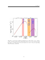
The Spectral Energy Distribution (SED) is usually plotted as the power emitted
at each frequency per logarithmic energy interval (νFν ) versus frequency (ν) on a
log-log plot. Also called a “power spectrum”, it is an easy and compact way to view
information about the frequency distribution of the emitted power across the entire
electromagnetic spectrum in one plot.
As mentioned above, the SED of blazars exhibits two broad peaks (see Fig. 2.8).
21
Future Observat
IACT
GLAST
X-ray
2.4 Blazars
F
s
c
m
a
o
V
o
Figure 2.8: Typical Spectral Energy Distribution for AGN. There are two distinct
peaks: one in the optical to X-ray band and the other in γ-rays. Colored bars represent
the ranges over which various detection methods are used: X-ray, the upcoming
GLAST satellite, and IACTs.
Blazar SED model using SSC code
22
G
2.4 Blazars
The first peak is usually in the optical-to-X-ray band, and almost universally attributed to synchrotron emission. The second peak occurs in the MeV-to-GeV band,
but there is still much speculation as to what causes this emission. The most accepted
mechanism for this second peak is inverse Compton emission. Various theories are
discussed further in Section 2.4.2.
Since the flux from blazars varies considerably over time, their SEDs are also
changing. When BL Lac sources get brighter, the emission peaks shift to higher
energies. Using computer code to model blazar emission developed by Coppi (1992),
we have seen the SED peaks evolve over time as the simulated blazar goes through
flaring cycles. Such shifts have been also observed, for example, in Mrk 501 (Pian
et al., 1998).
2.4.2
Emission Models and Particle Acceleration
Several theories have been presented to account for the unique SED of blazars.
More observations, in particular simultaneous observations at many different wavelengths, are necessary to break the model degeneracies and prove the mechanism by
which particles are being excited to such extremely high energies.
Synchrotron Self-Compton
The Synchrotron Self-Compton (SSC) model was originally proposed by Ginzburg
and Syrovatskii (1969). It has since been expanded for spherically homogeneous
sources and evolved to incorporate relativistic jets. It is the simplest explanation for
23
2.4 Blazars
blazar emission, in that the same population of relativistic electrons is responsible
for both the X-ray and γ-ray peaks of the SED. The blazar’s strong magnetic field
accelerates the electrons in its jets which radiate synchrotron photons in the process,
creating the lower SED peak. Inverse Compton processes then cause the upper peak,
as these radiated photons collide with the same relativistically accelerated electrons
that created them in the first place.
The most basic version of this scenario is the one-zone model, where emission
comes from a shock front moving along the jet (Sikora and Madejski, 2001). This
emission zone has a homogeneous magnetic field and proceeds relativistically down
the jet, as electrons are constantly injected. The resulting spectrum of relativistic electrons can be described by a broken power law with a shoulder at the break
frequency νB .
External Compton
Similar to SSC, External Compton (EC) models involve the same group of relativistic electrons radiating at lower energies by synchrotron radiation and at higher
energies by inverse Compton (IC) radiation. However, the difference lies in the fact
that the dominant seed photons for the IC emission come from outside the jet, and
are not the same photons already being radiated through synchrotron processes. If
the Compton scattering of ambient photons dominates the SSC emission, the energy
density of the external radiation (measured in the jet frame) must exceed the energy
density of the jet-produced synchrotron radiation. This requires the ambient photons
24
2.4 Blazars
to be upscattered far from the source of synchrotron radiation (≥ 1017 cm), so the
newly created γ-rays are not lost to absorption by thermally emitted photons through
pair production (Maraschi et al., 1992).
Hadronic Models
This theory involves a population of protons with very high (> 1017 eV) energy
being created near the core of the AGN that travel down the jets. An intense proton
flux near the jet base produces pions, both neutral and charged, which decay into
γ-rays and electrons, respectively. These high energy electrons (> 1016 eV) produce
synchrotron radiation, which becomes a large portion of the γ-rays one observes. In
this model, the X-rays, also produced through synchrotron radiation, come from a
completely different population of electrons, those generated by the blazar’s magnetic
fields within the jets, as with the other two models.
Particle Acceleration
To produce any of the above-mentioned emission, the electrons/positrons may be
accelerated by shocks in the jet (see review by Kirk and Duffy, 1999). For example,
some (Sokolov and Marscher, 2005; Mimica et al., 2004) suggest electrons are accelerated as they pass back and forth across the interface where two relativistic shock
fronts collide. Alternatively, the particles may be accelerated by the central engine
itself (Levinson, 2005; Katz, 2006; Krawczynski, 2006).
Many authors (Piner and Edwards, 2005; Henri and Saugé, 2006; Tavecchio, 2005)
25
2.4 Blazars
have investigated the “Γ problem”, wherein previous simulations of SSC emissions
require a bulk Lorentz factor ∼ 25, an order of magnitude higher than what is observed through VLBA (Very Long Baseline Array) observations. Ghisellini et al.
(2005) get around this need for high Lorentz factors by assuming there is a “layer
and spine” structure to the AGN jets. Here, two concentric volumes move at different velocities, and therefore boost the emission seen by a factor of ∼ (Γ0 )2 =
Γ2spine Γ2layer (1 − βspine βlayer )2 . The lower bulk Lorentz factors required by this model
are more in line with the radio observations.
2.4.3
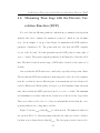
Markarian 421
For this study, we looked at the known TeV blazar Markarian (Mrk) 421. This
source is a nearby (z = 0.031), high-energy peaked BL Lac object. It was the first
extragalactic source detected in the TeV γ-ray band (Punch et al., 1992). It is also
visible in the Northern Hemisphere in spring, when the data were taken; the Crab
Nebula, the standard candle for γ-ray sources, is only visible there in the fall.
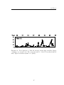
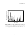
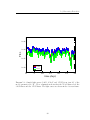
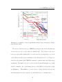
Mrk 421 is a very active source, frequently prone to flaring, sometimes to brightness levels exceeding 10 times that of the Crab Nebula. Figure 2.9 shows its light
curve in X-rays over several years. Mrk 421 shows loose correlation between the X-ray
and TeV γ-ray bands, and has been the subject of many previous multiwavelength
campaigns (e.g. Blażejowski et al., 2005; Takahashi et al., 2000). The history and
volume of knowledge on Mrk 421 make it an appropriate candidate for testing the
new VERITAS system.
26
2.4 Blazars
153
H OBSERVATIONS OF 1ES 1959+650
ion, a
cult to
or inppi &
002).
d low
0 had
e (e.g.,
sellini
ported
with a
1999).
ns was
X-ray
tentav teleointed
ations
ase in
All Sky
scope.
are on
by the
Figure 2.9: X-ray lightcurve of Mrk 421 showing extreme flux variability (flares)
continuing over several years. The y-axis shows the 2 − 12 keV X-ray flux in mCrab
units. Figure from Krawczynski et al. (2004).
27
Chapter 3
γ-ray Detection and VERITAS
3.1
γ-ray Propagation
Very High Energy (VHE) γ-rays (∼ 1011 − 1013 eV) can come from both galactic
and extragalactic sources. Unlike GeV and TeV cosmic rays, which are isotropized
by galactic magnetic fields and bombard the Earth from all directions, VHE γ-rays
come from particular objects in the sky. Within the galaxy, these sources are mainly
pulsars, X-ray binary stars, or supernova remnants, while extragalactic sources are
usually blazars. One can easily pinpoint where the γ-rays are coming from because
they are uncharged and therefore their trajectories are unaltered by magnetic fields
that exist throughout space.
28
3.1 γ-ray Propagation
3.1.1
Propagation Through Space
The strength of extragalactic γ-ray signals is reduced by interactions with the
intergalactic infrared (IR) background in pair production processes
γVHE + γIR → e+ + e− .
(3.1)
The absorption is strong for a wide range of VHE γ-rays above ∼ 20 GeV, due to the
broad peak in energy of the absorption cross section. The peak occurs when
EVHE EIR (1 − cos θ) ∼ 2(me c2 )2 = 0.52 (MeV)2 ,
(3.2)
where EVHE and EIR are the energies of the VHE γ-ray and IR photon respectively,
and θ is the angle of the collision between the two particles. The mass of the electron
and speed of light in a vacuum are represented by me and c. For 1 TeV photons,
this peak occurs when colliding head-on with 0.5 eV photons. However, absorption is
strong across a wide range of energies due to the spectral features of the extragalactic
background (Gould and Schréder, 1967; Stecker et al., 1992).
3.1.2
Air Showers in the Atmosphere
VHE γ-rays > 300 GeV require detector areas much larger than the ∼ 1 m2 of
typical space-borne telescopes in order to have any chance of detection. This is not
technically or financially feasible. However, the Earth’s atmosphere is completely
opaque to such high energy particles. In order to detect γ-rays on the ground, one
must use an indirect technique.
29
Table 2.1: Shower characteristics for several primary gamma-ray energies. Data
from (Weekes, 2003), p 15.
3.1 γ-ray Propagation
!
e+
e−
!
e+
!
e−
!
!
e+
e−
Figure 2.3: Simple model for a gamma ray induced air-shower. The primary
3.1: When
γ-ray
interacts withstarting
the Earth’s
it pair-produces
gammaFigure
ray interacts
in athe
atmosphere,
an atmosphere,
electromagnetic
cascade. The
and initiates a cascading shower of electrons and positrons.
electrons and positrons produced in the interaction emit more gamma rays via
bremsstrahlung, which pair-produce electrons and positrons. The process continues
γ-ray
Inducedfor
Showers
until the
threshold
pair-production is reached and the shower dies out.
While impossible in free space due to energy and momentum conservation (Longair, 1992), γ-rays can pair-produce in the Earth’s atmosphere, creating a cascading
35
shower of electrons and positrons. These in turn produce another high-energy photon
through bremsstrahlung, and the process repeats. Figured 3.1 schematically shows
this cascading air shower. The result is a tightly collimated beam of Čerenkov light
that eventually hits the ground.
30
3.1 γ-ray Propagation
Figure 3.2: A particle traveling
faster than the speed of light within a
medium emits Čerenkov radiation at
a specific angle given by Equation 3.3.
Figure from http://wikipedia.org.
c
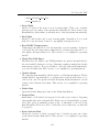
Čerenkov Radiation
When a particle travels through a medium at a velocity v faster than the speed
of light in that medium, Čerenkov radiation is produced. A “shock front” is created
and the particle radiates away energy. This results in a cone of Čerenkov light, which
has a fixed angle θC with respect to the direction of particle motion. This angle is
found by
θC = cos
−1
cm t
vt
= cos
−1
1
βn
,
(3.3)
where cm is the speed of light in the medium, and n is the index of refraction of that
medium. As usual, β = v/c. Figure 3.2 depicts this scenario graphically.
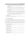
To visualize how this radiation manifests itself, consider first a charged particle
(like an electron) moving slowly through a medium. As it moves, the electron polarizes
the nearby atoms, pushing the negative charges away from it (see Fig. 3.3a). The
atoms relax back to their normal configuration after the electron has passed. Because
the speed of the electron is relatively slow, this produces a symmetric disturbance in
31
3.1 γ-ray Propagation
A
A
11
00
00
11
00
11
00P
11
−
−
+
+
−+ − +
+
+
−
−
−
+
− −
− + + −
+ − − +
+ + +
+
+ + −
−
+ − −
+
− −
+ +
+ +
−+
+−
11
00
00P
11
00
11
00P
11
−
−
+
+ − +−
+
+
−
−
P+
1
1
11
00
00P
11
11
00
00P
11
2
2
B
B
Figure 3.3: a) When a charged particle travels slowly through a medium, it polarizes
the surrounding atoms. b) When the particle moves faster than the speed of light in
the medium, there is a build-up of polarized charge just behind the moving particle.
Figure adapted from Jelley (1958).
the medium, so no net polarization is observed.
However, if the charged particle is traveling faster than the speed of light in
the medium, the polarization of nuclei is not symmetric (see Fig. 3.3b). The moving
particle’s charge is not propagated to the atoms of the medium until after the particle
has passed, creating a build-up of positive charge just behind the moving electron.
The transmittance of the electron’s charge is sent out radially, and becomes cohesive
along a wavefront at the angle θC from the direction it is traveling.
In air, the Čerenkov light reaching the ground has its peak emission in the UV/blue
32
3.2 Detection Using an Imaging Atmospheric Čerenkov Telescope (IACT)
portion of the spectrum. Telescopes that observe Čerenkov light are designed to have
peak efficiency in this range.
Cosmic Ray Induced Showers
Cosmic rays are also constantly bombarding the Earth, and they too produce
cascading showers in the atmosphere. This hadronic shower is much different than
showers produced by a γ-ray, and includes both pions and muons. Hadronic showers
are spread out over much larger areas than electromagnetic showers, owing to the
momentum of the nucleons and quarks that give rise to large transverse velocities
of the secondaries of hardronic interactions. Figure 3.4 shows schematically how a
cosmic ray shower propagates through the atmosphere.
3.2
Detection Using an Imaging Atmospheric Čerenkov
Telescope (IACT)
3.2.1
Atmospheric Technique
While the Earth’s atmosphere has negative effects on most astronomical observations, with clouds and air currents distorting an astronomer’s view of the heavens,
it is a very necessary component for ground-based γ-ray observations. In fact, one
is using the atmosphere as the detector medium to greatly increase the apparent
collection area for such a telescope. The main drawback of using the atmosphere is
33
3.2 Detection Using an Imaging Atmospheric Čerenkov Telescope (IACT)
2.1 Atmospheric Čerenkov Telescopes
p
"0
"#
!µ
"+
$
$
Nucleon Cascade
µ#
e−
e+
e−
!µ
e+
µ+
EM Cascade
EM Cascade
!µ
!e
e−
!e
e+
$
!µ
e−
$
e+
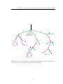
EM Cascade
EM Cascade
Figure 2.4: A model of a cosmic-ray-induced (hadronic) air-shower. (Figure
adapted3.4:
fromA(Jelley,
Figure
cosmic1958))
ray induced air shower is much more extended than that of a
γ-ray induced shower. Figure adapted from Jelley (1958).
37
34
3.2 Detection Using an Imaging Atmospheric Čerenkov Telescope (IACT)
its unpredictability. Its transparency affects the amount and angular distribution of
Čerenkov light seen on the ground. Cloud layers can cause errors in the data including a higher detection threshold and inaccurate energy reconstruction. Hence, data
must be taken on clear nights to be completely effective.
3.2.2
Imaging Čerenkov Radiation
When trying to observe a γ-ray source in the night sky, most of one’s view is
dominated by background noise and cosmic ray induced showers. Čerenkov light is
only visible as a very weak (∼ 50 photons m−2 ), very short (∼ 5 ns) pulse. While
the intensity of the shower requires highly sensitive electronics to record, the pulse
duration is what allows us to distinguish them from much of the night sky background.
Many methods have been utilized to better discriminate between the γ-ray signal
and background. The biggest advancement in this field came with the development
of technology to image the individual air showers. A camera with several individual
PMT pixels can be used to determine both the size, shape, and intensity of the shower.
Due to the differences in the lateral spread of various air showers, they can lead
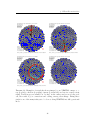
to quite different looking images when seen from the ground. Figure 3.5 shows the
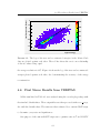
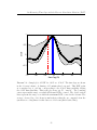
difference between a γ-ray induced shower and a cosmic ray induced shower propagating through the Earth’s atmosphere. γ-rays produce a very small, tight, round
image on the camera, while hadronic showers produce a larger, broader shape. This
difference is caused by the transverse momentum of nucleons and mesons present in
cosmic ray showers, but not in γ-ray showers.
35
3.2 Detection Using an Imaging Atmospheric Čerenkov Telescope (IACT)
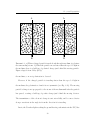
Figure 3.5: γ-ray induced air showers are very tight (left), while cosmic ray induced
air showers are much broader. Both simulated showers were initiated by a particle of
energy 100 GeV. Red lines represent electrons, positrons, and photons, and green and
blue lines represent muons and hadrons respectively. Images courtesy of F. Schmidt,
“CORSIKA Shower Images”, http://www.ast.leeds.ac.uk/fs/showerimages.html.
36
3.3 VERITAS: Very Energetic Radiation Imaging Telescope Array System
3.3
VERITAS: Very Energetic Radiation Imaging
Telescope Array System
VERITAS, an array of four IACTs, is currently being built at the base camp of
the Whipple Observatory in southern Arizona. It is designed as a successor to the
previous Whipple 10 m telescope still in operation on Mt. Hopkins. Being a nextgeneration telescope, VERITAS improves over Whipple in sensitivity and background
rejection (Weekes et al., 2002).
3.3.1
Telescope Array
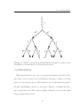
VERITAS is not just one, but several γ-ray telescopes that act together with a
single trigger to greatly increase background rejection in the data. Originally planned
as a grouping of seven identical telescopes, budget cuts required scaling back to just
four.
Due to several factors outside of the control of the VERITAS Collaboration, the
telescopes are initially being built on a temporary site at the Whipple Observatory
base camp. This put many restrictions on the construction process, so that the optimal telescope configuration could not be obtained. Originally, the four telescope
arrangement would have had one telescope in the center, and the other three equidistant from each other in a ring around the central telescope. The current configuration
resembles a trapezoid (see Fig. 3.6).
The four telescope array is still being constructed and tested. Telescope 1 began
37
3.3 VERITAS: Very Energetic Radiation Imaging Telescope Array System
Figure 3.6: The current configuration of the four telescopes at the base camp of
the Whipple Observatory is as shown. Distances and locations are not optimal due
to construction restrictions around the existing structures.
38
3.3 VERITAS: Very Energetic Radiation Imaging Telescope Array System
operating as a prototype in 2004 with half of its PMTs and one third of its mirrors,
and became fully operational in February, 2005 (Holder et al., 2006). Telescope 2
saw first light in September, 2005. The first two telescopes operated separately for
several months. The stereo trigger became active and the two telescopes operated
together as one starting in March, 2006. Construction on the other two telescopes
has progressed rather quickly, with Telescope 3 coming online in Fall, 2006, and
Telescope 4 in January, 2007.
The four telescopes are identical. Each consists of a 12 m diameter support structure holding a segmented reflector made up of 350 hexagonal mirrors of total area
∼ 110m2 arranged in a Davies-Cotton configuration (Davies and Cotton, 1957). These
focus incoming light onto the PMT camera, described in Section 3.3.2. Each telescope also has an electronics shed located right next to it. The sheds house the high
voltage supplies and controls, the digitizing electronics that convert the camera signal
so it can be processed, and the Level 2 trigger system. Figure 3.7 shows one of the
VERITAS telescopes and its electronics shed.
These four telescopes send output to a central control hub, which combines the
information from all telescopes into the final data stream. This is also the location
from which nightly observations are commanded.
3.3.2
Camera
Mounted on each telescope is a camera consisting of 499 individual photo multiplier tubes (PMTs). Each acts as a single pixel to image the air showers. These
39
3.3 VERITAS: Very Energetic Radiation Imaging Telescope Array System
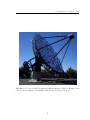
Figure 3.7: Pictured here is one of the four VERITAS telescopes in southern Arizona. The support arms extending off the 12 m optical structure hold the PMT
camera. When not in use, the camera rests at an access platform directly above the
electronics shed.
40
3.3 VERITAS: Very Energetic Radiation Imaging Telescope Array System
Figure 3.8: Each VERITAS
camera consists of 499 PMT pixels that cover a 3.5◦ diameter field
of view.
PMTs have their peak sensitivity in the blue/UV to maximize their sensitivity to
Čerenkov light. The entire camera housing is 1.8 m square, large enough to allow for
future expansion. The camera has a 3.5◦ diameter field of view. Figure 3.8 illustrates
the PMT camera.
Light cones are used to maximize the photon collection efficiency, by focusing light
onto the PMTs that would otherwise fall between them. They also shield the camera
from stray background photons that do not originate from the source direction. A
final design has now been chosen, but at the time the data for this thesis were taken,
Telescopes 1 and 2 had light cones of different designs. This fact does not adversely
affect this early stereo data.
The PMTs are operated with a gain of ∼ 2×105 electrons/photoelectron, necessary
to detect single Čerenkov photons from the air showers. The high voltage system to
bias the PMTs is housed in the control shed, next to each telescope.
41
3.3 VERITAS: Very Energetic Radiation Imaging Telescope Array System
The pre-amplifier attached to the base of each PMT is set up to allow constant
monitoring of the PMT currents, as well as to inject charge pulses into the system
for calibration and testing purposes. The current monitoring system allows for the
auto- or manual suppression of individual channels with high currents owing to faulty
electronics or a star in the field of view.
3.3.3
Trigger
In order for an event to register and be fully processed, it must pass a three-level
triggering system. These correspond to triggering on the pixel, telescope, and array
levels. The first level (L1) consists of fast constant fraction discriminators (CFDs)
processing the analog PMT signals. The CFDs contain a programmable 6 ns delay
to compensate for different PMT transit times and cable lengths.
From the CFDs, the L1 triggering signals are sent to the Level 2 (L2) trigger.
This is a topological system that uses a programmable look-up table of patterns to
determine if a given number of neighboring pixels have triggered. Currently, the
coincidence condition requires three neighboring pixels to trigger within 10 ns.
Each telescope L2 trigger is then sent to the Level 3 (L3) trigger. For the twotelescope data used for this thesis, the L3 trigger was set to require both telescopes
to record an event within a 100 ns coincidence window. This relatively wide window
ensured the array would trigger even if there were some problems with timing between
the two telescopes. If an event passes the L3 trigger, it is tagged with the GPS time
and the event is then read out from the data acquisition system.
42
3.3 VERITAS: Very Energetic Radiation Imaging Telescope Array System
3.3.4
Data Acquisition
One of the technical strengths of VERITAS is the data acquisition system. At
its heart is the 500 MHz flash ADC (FADC) system (Buckley, 1999). The signal
from each PMT is digitized in 2 ns bins and stored with a total lookback memory
of 32 µs. The FADC system allows for continuous data-taking while the triggering
system determines the validity of events, as well as the possibility for advanced timing
studies of the individual showers.
The FADC boards record data until they receive a signal from the L3 trigger that
an event has occurred. The data aquisition pauses until the relevant data are read
out, then continues digitizing data until the next event.
One important feature of the FADC boards is their ability to switch between a
high and low gain signal path. If a pulse comes through the FADC that exceeds the
dynamic range of the high gain path, a high/low gain switch is flipped, and the signal
from the low gain path is digitized. This allows the system to easily handle a wide
variety of pulse heights with an 8-bit digitizer.
43
Chapter 4
Mrk 421 Data Analysis
4.1
Event Reconstruction
The images captured by the VERITAS cameras result from thousands of bremsstrahlung and pair-production interactions in the atmosphere. To gain information
about the incident γ-ray, one must “reconstruct” an event and determine a number
of parameters characterizing the air shower. The important result of the event reconstruction is the location and orientation of the air shower axis, which points back
to the arrival direction of the primary γ-ray. Furthermore, the event reconstruction
gives information about the nature of the primary particle, photon or hadron. Last
but not least, we want to know the energy of the primary γ-ray. In the following, we
describe the methods used in this thesis.
44
4.1 Event Reconstruction
4.1.1
Hillas Parameterization
Čerenkov light reaching the telescopes’ cameras is captured by the individual
pixel PMTs. The resulting image can then be parameterized. Calculations of the
first, second, and third moments of the image distribution are used to fit an ellipse
to each event’s image. This process is described more fully in Reynolds et al. (1993).
The resulting parameters describing the size (length and width), placement (distance and miss) and orientation (α) of the ellipse are known as Hillas parameters.
Figure 4.1 shows these parameters in detail. Additional parameters used include
size, the total number of digital counts in the image. This is directly related to the
shower’s energy.
One great advantage to analyzing images this way is that air showers caused by
different particles look dramatically different in the camera. Since more than 99%
of the events recorded come from cosmic ray showers, it is beneficial to be able to
distinguish them from the more important γ-rays in the data. γ-ray initiated showers
create an ellipse with its major axis pointing towards the camera’s center. The large
transverse momentum associated with the strong hadronic interactions cause cosmic
ray showers to create a more rounded concentration of light. Muons, on the other
hand, produce a large ring, resulting from the initial interaction occurring relatively
close to the camera itself. Any other odd shape is just background noise. Figure 4.2
shows examples of these different types of events for one VERITAS camera. These
differences in shape allow for more efficient rejection of background events based on
45
4.1 Event Reconstruction
dth
wi
th
g
len
dis
i
g
a
m
is
ss
mi
x
ea
tan
ce
!
camera center
Figure 4.1: Illustration of the various Hillas parameters.
46
4.1 Event Reconstruction
values for the different Hillas parameters.
4.1.2
Stereo Reconstruction
After an event has been parameterized for each telescope, the images are combined
into one stereo event. This “stereo reconstruction” involves using the intersection of
the major axes of the ellipses of all telescopes to find the shower direction and axis
(see Fig. 4.3). From this reconstruction, we gain a new parameter, θ2 , the square of
the angular distance of the shower core from the center of the camera. Cutting on
this distance is the most reliable way to discard the maximum number of background
events while keeping as much signal as possible.
An important parameter we derive from the analyzed data is the mean scaled
width (M SCW ), which also proves to be very useful in separating hadronic from γ-ray
showers. M SCW —and its similarly derived cousin, mean scaled length (M SCL)—
utilize the fact that hardronic showers appear significantly “wider” in an IACT camera, due to the transverse momentum associated with the nucleons and mesons as
their interactions cascade through the atmosphere. Using Monte Carlo simulations
(see Sect. 4.5), we create a look-up table of expected median width values (wm ) and
the 90%-widths of the distributions (w90 ) as functions of both size and r, the distance
of the telescope from the shower axis. From these tables, we calculate a “normalized
width”

M SCW =
1
Ntrig

X widthi − wm (ri , sizei )
,
×
w
(r
,
size
)
90 i
i
i
Ntrig
(4.1)
summing over all Ntrig telescopes with a trigger, where widthi and sizei are the width
47
4.1 Event Reconstruction
Run: 1986 Event: 87 Type: 0 GPS: 2005 333 : 5 : 59 : 57.33772
Max channel 500
Num Samples 24
Num Trigger 36
Num Tubes 53
Num Dead 42
Run: 1986 Event: 129 Type: 0 GPS: 2005 333 : 5 : 59 : 57.67546
Max channel 500
Num Samples 24
Num Trigger 19
Num Tubes 35
Num Dead 42
Primary: 0
Energy [TeV]: 0.00
X: 0.00 Y: 0.00
Xcos: 0.000 (Ze: 0.00)
Ycos: 0.000 (Az: 0.00)
Primary: 0
Energy [TeV]: 0.00
X: 0.00 Y: 0.00
Xcos: 0.000 (Ze: 0.00)
Ycos: 0.000 (Az: 0.00)
T1
T1
GEO: c_x=-0.06, c_y=1.08, dist=1.08, length=0.3622, width=0.1738, α =4.57, size=8053.92
GEO: c_x=0.10, c_y=-1.06, dist=1.06, length=0.4172, width=0.1433, α =4.80, size=1749.40
Run: 1986 Event: 429 Type: 0 GPS: 2005 333 : 5 : 59 : 59.68064
Max channel 500
Num Samples 24
Num Trigger 35
Num Tubes 53
Num Dead 42
Run: 1986 Event: 140 Type: 0 GPS: 2005 333 : 5 : 59 : 57.73382
Max channel 500
Num Samples 24
Num Trigger 5
Num Tubes 0
Num Dead 42
Primary: 0
Energy [TeV]: 0.00
X: 0.00 Y: 0.00
Xcos: 0.000 (Ze: 0.00)
Ycos: 0.000 (Az: 0.00)
Primary: 0
Energy [TeV]: 0.00
X: 0.00 Y: 0.00
Xcos: 0.000 (Ze: 0.00)
Ycos: 0.000 (Az: 0.00)
T1
T1
GEO: c_x=0.46, c_y=-0.17, dist=0.49, length=0.7211, width=0.6233, α=17.56, size=3142.10
Figure 4.2: Examples of actual sky shower images by one VERITAS camera: a γray (top left), a hadron (top right), a muon (bottom left), and a noise event (bottom
right). Pixels in grey are marked as “broken” in the camera and are not being read
out, the result of poor connections and cabling, among other things. Fixing these
pixels is one of the many tasks yet to be done to bring VERITAS into full operational
mode.
48
4.1 Event Reconstruction
356
EA. Ahuronian
et al. /Astroparticle
*Shower
core
CT- 2
Physics 6 (1997) 343-368
CT-i
\
tl. laegrzel
CT-4
Fig. 9. Reconstruction
of the arrival direction of showers. The shower impact point on the ground is defined through the angles 61:. fib
in the focal plane which determine 3-dimensional angles ri, CT @i and rb ru 01 for @.r,y = sin O,,, << 1 (left figure). Note that the
image Distance parameter is defined as di = ( (01)’ + (O$)*) ‘I*. The camera planes are all parallel but not lying in a common plane.
To determine the shower direction the images in all cameras are superposed (right figure). Solid ellipses correspond to a shower with
direction parallel to the telescope axes, and dotted ellipses correspond to a shower inclined by angle 8.
Figure 4.3: Reconstructing the arrival direction of stereo showers. The shower
impact point and the resulting images in each camera are shown on the left. The
images from each camera are then superimposed (right). Solid ellipses portray a
shower vertically incident to the telescopes; dotted ellipses correspond to a shower
inclined by an angle θ0 . Figure from Aharonian et al. (1997).
I
I(XiGeV
?
31x1GeV
3
I TcV
n.2
0 25
J
-0.4
-0.2
0
02
0.4
Ox
Fig. 10. Angular
resolution
[degree]
0.6
49
0
0.05
0.1
0.15
of the IACT ‘cell’ at different energies of primary y-rays.
0.3
0 15
(I 4
0 s
BcrIdegreel
115
4.1 Event Reconstruction
and size values for the image in the ith telescope, and ri is that telescope’s distance
from the shower axis. M SCW is more useful than simply looking at width distributions for multiple telescopes, because it takes into account the shower’s location
relative to each of the telescopes, weighting the individual width distributions by the
appropriate factor to calculate this normalized parameter.
Monte Carlo simulations are also useful to help reconstruct the energy of the γ-ray
shower. We can create a look-up table of energies using the median and 90%-width
values of the logarithm of the size parameters as a function of the primary shower’s
energy E. To reconstruct the energy of a shower, we simply invert the table. The
shower’s reconstructed energy is determined by averaging the energies obtained from
each telescope with a trigger.
4.1.3
Analysis Tools
As VERITAS is still fairly new, there is yet no fully established method for data
analysis. The official analysis package, VEGAS (VERITAS Experiment Gamma-ray
Analysis Suite), is still in development and far from fully optimized or simple to use.
Using VEGAS will soon become standard, but for this work we have relied on other
packages that have been more thoroughly tested and are known to produce reliable
results for γ-ray data.
To analyze the data, we have used the University of Leeds’ eventdisplay and
mscw energy packages. These packages handle the main aspects of data reduction
and analysis for a stereo system. The programs’ output files can be imported into
50
4.2 Data Cuts and Significances
ROOT for further analysis and plotting. The eventdisplay package also contains extensive display tools to view individual events on each camera, as well as individual
FADC traces and other timing information.
For each night of data, a calibration must be done to correct for minor fluctuations
in weather and telescope electronics. This is done through the use of a “laser run”.
At the start of each night, a short run is taken where a laser is flashed at the PMT
camera. The constant flux of these pulses is used to adjust the analysis program to
the subtle differences in how each pixel detects the light intensity as well as timing.
After the calibration is done, each run for the night may be analyzed and parameterized. Hillas parameters are calculated for each telescope, and the stereo data is
reconstructed to find the shower axis (see Sect. 4.1.1). Afterwards, the mean scaled
width, mean scaled length, and energy are reconstructed.
4.2
Data Cuts and Significances
After the events are fully parameterized, cuts are applied to separate actual γ-rays
from background events. Once VERITAS is brought fully online and more data have
been acquired and analyzed, a standard set of cuts will become available. Since the
standard cuts have yet to be established, we present preliminary work to establish
cuts in both M SCW and θ2 , discussed in Section 4.6.
To determine the excess, one separates the events passing all data cuts into two
categories: events from the signal or “ON” region, and events from a comparison
51
4.3 Spectral Reconstruction
background or “OFF” region (see Sect. 4.4.1 for more on these regions). The number
of events in these regions (NON and NOFF respectively) can be used to calculate the
γ-ray rate as well as its associated error:
NON − NOFF
±
r ± ∆r =
time
√
NON + NOFF
.
time
(4.2)
A large positive excess of at least the 5σ level means the source has been detected.
This statistical significance is calculated as follows:
σ=
4.3
r
NON − NOFF
=√
.
∆r
NON + NOFF
(4.3)
Spectral Reconstruction
Spectral reconstruction of the Mrk 421 data was performed using the forwardfolding method of Henric Krawczynski, described fully in Rebillot et al. (2006). It
has been incorporated into the program wufit, part of Washington University’s own
data analysis package, wuparam.
Energies are reconstructed for every event in both the ON and OFF regions, as
well as for all Monte Carlo simulated events, as described above. The energies are
histogrammed, and the OFF energy histogram is subtracted from the ON energies
to yield the energy excess. The energy spectrum can then be fitted to the excess
histogram, with help from the Monte Carlo simulated energy histogram, using the
forward-folding approach (see, e.g., Fenimore et al., 1982).
52
4.4 Mrk 421 Data from April–May 2006
The data are fit using a power-law model:
dNγ
= N0 · (E/1 TeV)−Γ
dE
(4.4)
where N0 is the flux normalization at 1 TeV and Γ is the photon index. For each trial
parameter set (N0 and Γ), an energy histogram is filled weighing the Monte Carlo
events so as to mimic the model of Equation 4.4. Both parameters are then varied
in the user-defined parameter space to minimize the χ2 difference between the data
and Monte Carlo histograms. The values of N0 and Γ with the best fit, along with
associated errors, give the source’s energy spectrum.
4.4
Mrk 421 Data from April–May 2006
Data taken during the dark run from April–May 2006 were the first set of true
stereo data from the VERITAS telescopes. The data on the known blazar Mrk 421
contain a large number of γ-ray events and can be used for calibration purposes.
4.4.1
Observation Modes
There are a variety of modes in which VERITAS data can be taken. ON–OFF
pairs were the standard method in the past, however they require an extremely clear
sky to be useful because passing clouds will affect the source and background regions
differently. This method can seem wasteful in that half of the observation time is
used to examine blank fields in the sky. Tracking runs are useful because they require
less time than ON–OFF pairs and can still be effective in less than perfect weather,
53
4.4 Mrk 421 Data from April–May 2006
due to clouds altering both ON and OFF regions in the same way. The method is
somewhat problematic as the sensitivity is not uniform over the entire field of view
of the telescopes. We are also trying out an attractive method, Wobble mode, which
combines the benefits of both Tracking and ON–OFF pairs into a single method which
minimizes both the observation time and the systematic uncertainties.
ON–OFF Pairs
Frequently used on the Whipple 10 m telescope, ON–OFF pairs are good for
getting high quality data, but are only accurate and effective on cloudless nights.
First, a 28-minute run is taken with the source at the center of the camera. Then, a
second OFF run is taken, offset 30 minutes in Right Ascension, and taken 30 minutes
after the ON run. This second run sweeps across the exact same portion of the sky
as the ON run for more accurate background subtraction that is not affected by the
systematics of the telescope itself. Many data from this dark run were taken as ON–
OFF pairs, but have been processed as tracking to simplify the analysis procedure.
Tracking Runs
Tracking runs require less time and can be useful in less perfect weather. These
runs simply keep the source at the center of the camera at all times. For background
subtraction, an OFF region is chosen farther from the center of the camera, so it is
not be affected by the source itself. Figure 4.4a depicts visually the ON and OFF
regions of the field of view for a Tracking run. The ON region is a circle with given
54
4.4 Mrk 421 Data from April–May 2006
Tracking
Wobble
ON
0.3°
camera
center
Area(ON) =
Area(OFF)
OFF
Figure 4.4: The different observation modes have different ways in which background is subtracted from OFF regions. For tracking runs (left), the OFF region is
an annulus with the same area as the source region, spaced a bit outside of the source
region. For wobble runs (right), the OFF region is the same shape and size as the
ON region, but offset on the other side of the telescope’s center.
radius at the center of the camera. The OFF region is then an annulus with the same
area as the ON region, centered on the source, with a buffer zone of space between
the two, so the source does not contaminate the background region.
This method is less reliable than doing ON–OFF pairs for several reasons. Because
the OFF region is farther from the camera’s center, the number of events in this region
may be less than what one would expect. This could be due, in part, to these events
not triggering both telescopes. Also, because the centroids would occur at larger
distances from the camera center, the images could be more spread out, introducing
a bias in the width distributions. In contrast to ON–OFF pairs, passing clouds would
55
4.4 Mrk 421 Data from April–May 2006
effect both the ON and OFF regions in the same way, making this behavior a tradeoff
between the two methods.
Wobble Runs
Wobble runs have proved an effective observation mode for stereo Čerenkov telescope systems such as HEGRA (Daum et al., 1997) and H.E.S.S. (Aharonian et al.,
2005c) as the detection sensitivity is rather uniform over the central part of the field of
view. VERITAS is starting to use them as well. This method combines the effectiveness of ON–OFF pairs with the convenience and speed of a Tracking run. Wobbling
involves offsetting the source by a given amount in the field of view. The offsets are
in varying directions (usually opposite) in order to cancel out systematic inhomogeneities in the camera itself. Figure 4.4b depicts visually the ON and OFF regions
for a wobble run. Both regions are the same size and shape, offset on opposite sides
of the camera, with the ON region centered on the source. There is space between
the two regions, again, to prevent the source from influencing the background region.
This method is not as valuable for single telescopes, because their detection rate is
more strongly affected by stars in the field of view and faulty pixels.
4.4.2
Final Data Set
Not every data run that was taken is useable. Various problems exist with the
data as this new experiment is slowly brought completely online. Issues range from
imperfect weather, to rate spikes due to nearby car headlights, to issues with the
56
4.4 Mrk 421 Data from April–May 2006
hardware and software.
Ground-based γ-ray telescopes usually operate at around a 10% duty cycle. The
solar and lunar cycles (especially towards summer, as the number of daylight hours
increases) as well as the weather and Arizona’s monsoons severely limit the amount
of time it is possible to operate the telescopes.
After disregarding all runs with rate spikes, as well as those with irrepairable
problems, we were left with the final data set that was used to complete the following
analysis. A total of 32 runs over nine separate days, corresponding to 14.3 hrs of
observations, were used. Table 4.1 lists the data and laser calibration runs used.
Table 4.1: Run information that makes up the final data set from which this thesis
is based. Data runs are all of the source Mrk 421 during the April–May 2006 dark
run. Associated laser calibration runs are also listed. ON–OFF pairs are denoted as
“ON/OFF”, Tracking runs as “Trk”. Wobble runs denoted as the offset distance and
direction: “0.3N” implies the source is offset 0.3◦ to the North of the camera’s center.
Date
Run Number
2006-04-20
30336
2006-04-20
30328
2006-04-20
30330
2006-04-20
30333
2006-04-21
30358
2006-04-21
30365
2006-04-23
2006-04-23
2006-04-23
2006-04-23
2006-04-23
2006-04-24
2006-04-26
2006-04-26
2006-04-26
30404
30394
30396
30398
30400
30424
30476
30478
30480
OFF Run
—
30329
30332
—
30359
—
Laser Run
—
30336
30336
30336
30336
30336
Run Type
laser
ON/OFF
ON/OFF
Trk
ON/OFF
Trk
Elevation
—
83
78
67
82
69
—
30395
30397
30399
30401
—
30477
30479
—
—
30404
30404
30404
30404
30404
30404
30404
30404
laser
ON/OFF
ON/OFF
ON/OFF
ON/OFF
Trk
ON/OFF
ON/OFF
0.3E
—
77
83
75
64
83
72
62
50
Continued on next page. . .
57
4.5 Comparison of Experimental and Monte Carlo Data
Table 4.1 – Continued
Date
Run Number
2006-04-27
30504
2006-04-27
30492
2006-04-27
30493
2006-04-27
30494
2006-04-27
30495
2006-04-27
30496
2006-04-27
30497
OFF Run
—
—
—
—
—
—
—
Laser Run
—
30504
30504
30504
30504
30504
30504
Run Type
laser
0.3E
0.3W
0.3N
0.3S
0.3N
0.3S
Elevation
—
82
77
70
64
58
52
2006-04-29
2006-04-29
2006-04-29
2006-04-29
2006-04-29
30540
30533
30534
30536
30537
—
—
—
—
—
—
30540
30540
30540
30540
laser
Trk
Trk
Trk
Trk
—
83
81
69
63
2006-04-30
2006-04-30
2006-04-30
2006-04-30
2006-04-30
2006-04-30
2006-04-30
2006-04-30
30564
30553
30554
30555
30556
30557
30559
30560
—
—
—
—
—
—
—
—
—
30564
30564
30564
30564
30564
30564
30564
laser
Trk
Trk
Trk
Trk
Trk
Trk
Trk
—
78
73
68
62
56
45
41
2006-05-01
2006-05-01
2006-05-01
30575
30570
30572
—
—
—
—
30575
30575
laser
Trk
0.3S
—
65
52
4.5
Comparison of Experimental and Monte Carlo
Data
In order for the energy spectrum or other results relying on Monte Carlo simulations to be reliable, one must first prove that the simulations accurately describe
58
4.5 Comparison of Experimental and Monte Carlo Data
the system they are intended to model. By comparing the distributions of the various parameters in the simulated data set to those from experimental data, one can
test how well the Monte Carlo simulations are performing and how accurate results
obtained with them will be. Here we use Mrk 421 as a strong “test beam” of γ-rays.
For this study, Monte Carlo simulations were done on vertically incident γ-rays
with energies from 30 GeV to 50 TeV. A total of 2,615,000 events with a Crab-like
differential spectral index of Γ = 2.5 were simulated. The showers were simulated
over an area of radius 350 m. While γ-rays behave differently when the telescope is
pointed at lower elevations than at higher ones (Kosack et al., 2004), the (generally)
low zenith angles of the runs used in this study did not require simulating different
zenith angles. Simulations were generated with the Grinnell-ISU (GrISU) package1
that uses the KASCADE air shower simulation code of Kertzman and Sembroski
(1994), followed by the simulation of the Čerenkov light emitted by the air shower
and the telescope detector’s response to that light.
Figure 4.5 shows several plots of the various Hillas parameters, comparing the
Monte Carlo simulations with real data. Overall, it can be seen that the two agree
very well, showing these simulations accurately model the air showers and the detector response. For both simulated and experimental data, only showers within a radius
of 200 m from the telescopes were used. Whereas most parameter distributions agree
very well over the entire range, the size distributions disagree at smaller size values.
This fact can be linked to both the steep spectrum of Mrk 421 and the difficulty in
1
See http://www.physics.utah.edu/gammaray/GrISU.
59
Normalized Entries
Normalized Entries
4.5 Comparison of Experimental and Monte Carlo Data
1
0.8
0.6
1
0.8
0.6
0.4
0.4
0.2
0.2
0
-0.2
0
0.1
0.2
0.3
0.4
0.5
0.6
0.7
-0.4
0.8
0.9
1
theta2 (degrees2)
Normalized Entries
Normalized Entries
0
1
0.8
0.6
-2
0
2
4
6
8
10
MSCW
9
8
7
6
5
0.4
4
0.2
3
0
2
1
-0.2
0
0.1
0.2
0.3
0.4
0.5
0.6
0.7
0.8
0.9
0
2.5
1
width
3
3.5
4
4.5
5
5.5
6
log(size)
Figure 4.5: Several plots showing both Monte Carlo simulated events (blue) as well
as real data events. The top two plots show array-level parameters, θ2 and M SCW ,
with the array data plotted in black. The bottom two plots show telescope-level data,
width and size, with T1 plotted in black and T2 in red.
modeling the trigger accurately. A cut of size > 1000 would eliminate this difference
between the two curves. We have also used these Monte Carlo simulations to estimate the energy thresholds, angular, core, and energy resolutions of the two-telescope
VERITAS experiment.
The energy threshold is calculated from the energy distributions of the Monte
Carlo simulations. Figure 4.6 shows these distributions both before and after the
optimized cuts discussed in Section 4.6. Where these histograms peak is commonly
referred to as the energy threshold. It is measured as 165 GeV before cuts, and
220 GeV after cuts.
60
Normalized Entries
4.5 Comparison of Experimental and Monte Carlo Data
1
0.8
0.6
0.4
0.2
0
-2
-1.5
-1
-0.5
0
0.5
1
1.5
2
log(Energy)
Figure 4.6: Plot showing the (log) energy distributions of the Monte Carlo simulations for a Crab-like spectrum of E −2.5 , both before (black) and after (red) cuts. The
energy bin with the most entries is the energy threshold: 165 GeV before cuts and
220 GeV after cuts.
One can also plot how the angular resolution of the simulations vary with energy.
For a given energy bin, the angular resolution is defined as the angular distance θ
below which occur 63% of the events. This resolution is plotted in Figure 4.7, and
Table 4.2 lists the values as well as the energy bins used. For the entire energy range,
the angular resolution is 0.29◦ in simulations.
Similarly, the core resolution can be plotted. This measures the difference in
position of the reconstructed shower core position from the actual position:
<core =
p
(xcore − M Cxcore )2 + (ycore − M Cycore )2 ,
(4.5)
where (M Cxcore , M Cycore ) is the true shower core and (xcore , ycore ) is the reconstructed core. eventdisplay can calculate the reconstructed core in two different ways:
61
Entries
4.5 Comparison of Experimental and Monte Carlo Data
1000
800
600
400
200
0
0
0.2
0.4
0.6
0.8
1
1.2
1.4
1.6
1.8
2
Angular Error (degrees)
Figure 4.7: Plot showing the angular resolution of the Monte Carlo simulations.
For all energies, the angle below which 63% of events occur is 0.29◦ .
Table 4.2: Angular Resolution for the Monte Carlo simulations over different energy
ranges.
Energy Bin
< 100 GeV
100 GeV − 800 GeV
800 GeV − 2 TeV
2 TeV − 10 TeV
all energies
62
Angular Resolution
0.37
0.29
0.22
0.22
0.29
Entries
4.5 Comparison of Experimental and Monte Carlo Data
8000
7000
6000
5000
4000
3000
2000
1000
0
0
20
40
60
80
100
120
140
160
180
200
Core Error (m)
Figure 4.8: Plot showing the core resolution of the Monte Carlo simulations of all
energies. This data yielded a core resolution of 12.5 m.
Method 1 intersects the major axes of the second moment ellipses, while Method 2
intersects the lines connecting the centers of gravity of the images with the source
locations. Method 1 works for all sources, both point sources and extended sources.
Method 2 works only for point sources but achieves a better resolution. Since Mrk 421
is a point source, we use only Method 2. Shown in Figure 4.8, we obtain a core resolution of 12.5 m over the full range of simulated energies.
The energy resolution is calculated using the true (Etrue ) and reconstructed (Erec )
energies of each Monte Carlo event2 as
<energy =
Erec − Etrue
.
Etrue
(4.6)
The value below which 63% of events occur is the energy resolution. For all events,
2
Note: For this preliminary analysis, we have not attempted to optimize the Energy Estimator
function.
63
Log(Reconstructed Energy)
4.6 First Stereo Results from VERITAS
2
1200
1.5
1000
1
0.5
800
0
600
-0.5
400
-1
200
-1.5
-2
-2
-1.5
-1
-0.5
0
0.5
1
1.5
2
Log(True Energy)
0
Figure 4.9: The logs of the true and reconstructed energies for the Monte Carlo
data are plotted against each other. The red line shows the one-to-one relationship
of the two values being equal.
the energy resolution is 34%. Figure 4.9 shows the log of the true and reconstructed
energies plotted against each other, also demonstrating the accuracy of the energy
reconstruction.
4.6
First Stereo Results from VERITAS
All the runs listed in Table 4.1 were analyzed using the eventdisplay package with
the standard default values. These output files were then processed with mscw energy,
also with the default values. The runs were then evaluated by a custom ROOT script
to determine γ-ray rates and significances.
One purpose of the custom ROOT script was to optimize cuts on θ2 and M SCW
64
4.6 First Stereo Results from VERITAS
for this data set. The optimization aims at maximizing the Q-factor, defined as
the γ-ray acceptance divided by the square root of the background acceptance for a
particular cut:
Aγ
Q= p
.
Abg
(4.7)
It scales with the statistical significance of weak signals obtained with a certain cut.
For the cut optimization, all runs are treated as tracking runs.
As this is the first data taken with the new stereo VERITAS system, many
aspects—pointing, point spread function of the optics, trigger nonuniformity and
biases, etc.—are not well understood. Despite this fact, the two-telescope data on
Mrk 421 are very good.
4.6.1
Cutting on θ2
The first cut to be optimized was θ2 , the square of the angular distance of the
reconstructed arrival directions of the primary γ-rays from the source direction. This
is the most important cut for stereo data, and is very powerful at removing background
events from the source signal.
Initially, a histogram is made of the θ2 values for all events passing a very weak
cut of M SCW < 1.0. This removes the most obvious background events, to make
the cut optimization cleaner. The resulting histogram shows a prominent peak close
to θ2 = 0, with a tail that decreases linearly as a function of θ2 . Since there should
be no excess at values θ2 > 0.4 deg2 , one can assume all contributions there are from
background events. We then fit a line to the histogram for 0.4 deg2 ≤ θ2 ≤ 1.0 deg2 ,
65
1400
Entries
Entries
4.6 First Stereo Results from VERITAS
1200
1000
1200
800
1000
600
800
400
600
200
400
0
200
0 0.1 0.2 0.3 0.4 0.5 0.6 0.7 0.8 0.9 1
theta2 [degree2]
0 0.1 0.2 0.3 0.4 0.5 0.6 0.7 0.8 0.9 1
theta2 [degree2]
Figure 4.10: Plots of θ2 , the square of the angular distance of the events from the
source position, for the Mrk 421 data. On the left, θ2 for all data (solid line) and OFF
data (dotted line). The line for OFF data was fit from the dark solid line, assuming
no excess for large θ2 . The right shows the residual excess in the θ2 distribution.
Here, a loose cut of M SCW < 1.0 was used.
and extrapolated it to small values of θ2 to represent all background events. This
fit is shown in Figure 4.10a, along with the total θ2 histogram. The “OFF line” was
subtracted from the full histogram, leaving behind the ON excess histogram, seen in
Figure 4.10b.
The Q-factor is then calculated for this residual histogram. Figure 4.11 plots the
Q-factor, as well as signal and background acceptances, versus the cut in θ2 . This
gives a maximum Q-factor QMAX = 2.87, with a signal acceptance of 54%, and a
background rejection of 97%. This equates to an optimal cut of θ2 < 0.025deg2 , corresponding to an angular resolution of the two-telescope VERITAS system of θ = 0.16◦ .
As evident in Section 4.5, our simulations appear to overestimate the angular errors,
as they yield a resolution of 0.29◦ . In these early observations with a new system,
66
3
1
Q-Factor
Acceptance
4.6 First Stereo Results from VERITAS
2.5
Figure 4.11: Plot of the Q-factor as
a function of the applied θ2 cut (solid
black line, right axis). Also plotted
are the signal acceptance (blue dashed
line) and background acceptance (red
dot-dashed line).
0.8
2
0.6
1.5
0.4
1
0.2
0.5
0
0
0 0.1 0.2 0.3 0.4 0.5 0.6 0.7 0.8 0.9 1
cut in theta2 [degree2]
much about the telescopes, including quality of pointing and mirror alilgnment, remains uncertain. Further study will allow us to understand these behaviors and
improve future simulations.
4.6.2
Cutting on Mean Scaled Width
The data are now processed through the custom ROOT script again. From here
we can optimize the cut on M SCW . Data that pass the θ2 -cut will be placed into
two separate histograms (ON and OFF), based on the reconstructed origin of the
primary γ-ray.
For this study, the ON region is a circle of radius 0.22◦ centered on the source. The
OFF region is an annulus of inner radius 0.4◦ . The complete histograms of M SCW
for both the ON and OFF regions are shown in Figure 4.12.
The Q-factor is then calculated on the residual histogram. Figure 4.13 plots the
Q-factor, as well as signal and background acceptances, versus the M SCW cut. This
67
Entries
4.6 First Stereo Results from VERITAS
7000
6000
Figure 4.12: Plots of M SCW for
the Mrk 421 data for ON data (solid
line) and OFF data (dotted line).
Here, a loose cut of θ2 < (0.22)2 was
used.
5000
4000
3000
2000
1000
0
5
10
15
MSCW
2.2
1
2
Q-Factor
Acceptance
0
-5
1.8
0.8
Figure 4.13: Plot of the Q-factor as
a function of the applied M SCW cut
(solid line, right axis). Also plotted
are the signal acceptance (blue dashed
line) and background acceptance (red
dot-dashed line).
1.6
1.4
0.6
1.2
1
0.4
0.8
0.6
0.2
0.4
0.2
0
-5
0
5
10
15
cut in MSCW
0
gives a maximum Q-factor QMAX = 2.15, with a signal acceptance of 61%, and a
background rejection of 92% for the cut of M SCW < −0.21.
4.6.3
Mrk 421 Light Curve
After the cuts on θ2 and M SCW were established, the data were processed again
using these cuts. This yielded an average γ-ray rate of 2.91 ± 0.07 γ min−1 after
68
TeV flux [arbitrary units]
4.6 First Stereo Results from VERITAS
16
14
12
10
8
6
4
2
53846
53848
53850
53852
53854
53856
date [MJD]
Figure 4.14: Light curve from the April–May 2006 dark run for Mrk 421. Each
data run is represented by one point on the graph. Error bars are on the one-sigma
confidence level.
cuts. Correcting for the cut efficiencies, the true rate inferred from these data is
8.83 ± 0.21 γ min−1 . The total significance was found to be 39σ for 14.3 hours of data.
The flux measured for each of these runs was used to produce a preliminary light
curve of Mrk 421, seen in Figure 4.14. Absolute flux calibration has yet to be done, but
by comparison to the Crab rate of ∼ 6 γ min−1 derived by Celik (2007), we estimate a
variable flux for Mrk 421 on the order of 1/2 that of the Crab. This high variability
can be seen between runs taken on the same night, even though Mrk 421 was not in
its most active state. Such variability over short time scales was evident in numerous
observations in the past with the Whipple 10 m telescope. The improved sensitivity
of VERITAS will ultimately provide much better measurements of this variability on
all time scales.
69
Flux (arbitrary normalization)
4.6 First Stereo Results from VERITAS
10-1
-2
10
-3
10
-0.6
-0.4
-0.2
0
0.2
0.4
0.6
0.8
1
log(Energy)
Figure 4.15: Reconstructed energy spectrum of the blazar Mrk 421 from the first
VERITAS stereo data.
4.6.4
Energy Spectrum
In order to get a more accurate energy spectrum, only ON–OFF pairs were used
in this process; Wobble and Tracking mode data were ignored. Due to the high
significance of these runs, the nine pairs of data during this dark run were enough to
generate a spectrum with small statistical errors. Data were fit to the Monte Carlo
energy histogram as described in Section 4.3. This resulted in the energy spectrum
shown in Figure 4.15. Based on our preliminary analysis, we get a spectral index of
Γ = 2.26 ± 0.06. For the Crab Nebula, the Whipple 10 m telescope gives Γ = 2.5 ± 0.1
(Rebillot et al., 2006). The results on Γ are comparable to previous results from earlier
experiments where Mrk 421 was in a high state, e.g. the Whipple 10 m (Krennrich
et al., 2002), HEGRA (Aharonian et al., 1999), and H.E.S.S. (Aharonian et al., 2005c).
70
Chapter 5
SSC Modeling of Blazar Emission
5.1
Rationale
The previous chapter describes the analysis of VERITAS observations of the blazar
Mrk 421. Extracting astrophysical results will require one to observe the source with
good observational coverage over the entire electromagnetic spectrum. Such intensive
multiwavelength observation campaigns are planned for the years 2007 and 2008. In
this chapter, we present a theoretical study relevant for such multiwavelength studies.
We explore whether X-ray measurements alone can be used to constrain the magnetic
field in jets. If this were possible, the combined X-ray and γ-ray measurements could
be used to break additional model degeneracies.
71
5.2 Measurement of the Jet Magnetic Field
5.2
Measurement of the Jet Magnetic Field
During the last decade, time resolved multiwavelength observations of blazars
have emerged as a powerful tool to study AGN jets. The most detailed data so far
comes from joint observations of satellite-borne X-ray telescopes (ASCA, BeppoSAX,
RXTE, XMM) and ground-based TeV γ-ray telescopes (CAT, HEGRA, Whipple); see
Krawczynski (2004), Krawczynski (2005), Tavecchio (2005), and references therein.
The tight correlation between the X-ray and TeV γ-ray fluxes found for the blazars
Mrk 421 and Mrk 501 (Buckley et al., 1996; Takahashi et al., 1996; Krawczynski et al.,
2000; Sambruna et al., 2000) is commonly taken as strong evidence for synchrotronCompton models in which a single population of electrons emits X-rays as synchrotron
emission and γ-rays as inverse Compton emission off synchrotron target photons.
Since the X-ray and γ-ray observations give complementary information about the
same high-energy electron population, it becomes possible, in principle, to break
model degeneracies.
A major goal of blazar observations is to determine the key parameters describing
the jet plasma, such as the bulk Lorentz factor Γ, the jet Doppler factor1 δj , the energy
densities of the magnetic field, the thermal particle component, and the relativistic
particle component. X-ray and TeV γ-ray observations reveal flux variability on time
scales of minutes, indicating that the emission originates very close (∼ 1016 cm) to
The jet Doppler factor is defined by δj−1 = Γ(1 − β cos (θ)) with Γ the bulk Lorentz factor of
the emitting plasma, β its bulk velocity in units of the speed of light, and θ, the angle between jet
axis and the line of sight in the observer frame.
1
72
5.2 Measurement of the Jet Magnetic Field
the central engine (Gaidos et al., 1996; Catanese and Sambruna, 2000; Krawczynski
et al., 2001). A measurement of the the jet properties at the jet-base would constrain
the processes of matter accretion and jet formation, and would establish a crucial link
between violent processes near a black hole of 10−5 (MBH /108 M ) pc radius and the
kpc-scale radio and X-ray jets.
While snapshots of the Spectral Energy Distribution (SED) constrain the parameters of emission models, there is no single source for which the model parameters have
been determined unambiguously. In the case of “red” blazars (MeV/GeV blazars),
the intensity of “external” radiation fields which supply the target photons for inverse Compton processes is not well constrained (see, e.g., Tavecchio et al., 1998, for
a summary of constraints that can be derived from the broadband SED). In the case
of “blue” blazars (TeV blazars), models are simpler as external radiation fields are
thought to be weak. However, a highly uncertain amount of extragalactic extinction owing to pair-production processes of TeV γ-rays interacting with intergalactic
infrared photons (Gould and Schréder, 1967; Stecker et al., 1992) renders the interpretation ambiguous.
Additional constraints can be derived from the temporal evolution of the broadband energy spectra that reflect the evolution of the electron energy spectra owing
to various physical processes. If synchrotron-Compton models do indeed apply, and
if synchrotron cooling dominates the energy losses of electrons, high energy electrons
will lose their energy more rapidly than low energy electrons. The flux variability at
higher energies should lead the variability at lower energies, and a measurement of the
73
5.3 Synchrotron Self-Compton Simulations
“time lag” between the flux variability observed in different bands should constrain
the magnetic field inside the jet plasma.
With this aim, various authors have used the Discrete Correlation Function (DCF)
of Edelson and Krolik (1988) to search for a time lag between fluxes measured in
different X-ray bands and to constrain the jet magnetic field. Unfortunately, the
measurements have not produced a clear verification of the basic picture. Based on
a four-day uninterrupted observation of the blazar Mrk 421 with the ASCA satellite,
Takahashi et al. (2000) used the DCF formalism to determine a time lag between
the 0.5 − 1 keV and 3 − 7.5 keV fluxes. Rather than revealing a constant time lag
indicative of synchrotron cooling of electrons in a certain magnetic field, the analysis
showed that the time lag changed constantly in its value and its sign.
Based on four XMM observations of ∼ 10 hrs duration, Sembay et al. (2002)
performed a DCF analysis and derived an upper limit on the time lag between the
soft (0.1 − 0.75 keV) and hard (2 − 10 keV) emission of 300 sec. This upper limit
translates into a lower limit on the magnetic field of 2 (δj /10)−1/3 G, uncomfortably
high for synchrotron-Compton models.
5.3
Synchrotron Self-Compton Simulations
We use the time dependent SSC code of Coppi (1992) to create artificial data
sets. The code assumes a spherical emission region of radius R that approaches the
observer with a bulk Lorentz factor Γ. The emission volume is filled with an isotropic
74
5.3 Synchrotron Self-Compton Simulations
electron population and a tangled magnetic field of mean strength B.
We create a light curve by changing the rate of freshly accelerated electrons N0 (t).
We assume an electron acceleration spectrum following
dNe /dγ = N0 (t) × γ −p × exp (−γ/γmax )
(5.1)
with a spectral index p = 2, and a high-energy cutoff γmax that is constant for each
single simulation. The code self-consistently evolves the coupled partial differential
equations describing the energy spectra of the the non-thermal electrons and photons,
taking into account synchrotron emission and self-absorption, as well as continuous
and non-continuous energy losses owing to inverse Compton processes in the Thomson
and Klein-Nishina regimes, respectively. The photon density evolves as
c
∂nγ
= qγ − p γ −
nγ ,
∂t
R(1 + κ)
(5.2)
where qγ d and pγ d are the rate of photons being produced inside and outside the
energy interval [, + d], while the last term represents photons escaping from the
emission region. The electron density evolves as
∂ne
∂
ne
= Qe −
[γ̇cont ne ] + qe − pe −
,
∂t
∂γ
te,esc
(5.3)
where Qe (γ, t) is the rate of freshly accelerated electrons, γ̇cont is the decrease in an
electron’s Lorentz factor and qe dγ and pe dγ are the rates of particles being produced
or scattered inside and outside the Lorentz factor interval [γ, γ + dγ] (Krawczynski
et al., 2002). The SSC code assumes that the synchrotron emission provides the
dominant target photon field.
75
5.4 Generating Data Sets
Mimicking the duration of a typical multiwavelength observation campaign, we
generated artificial data sets of 30 days duration (observer frame). The first 10 days
were discarded from subsequent analysis so that the target photon fields and lowenergy electron distributions could reach a steady level. We created each artificial
data set by a series of N triangle bursts of accelerated particles:
N0 (t) =
N
X
Ai h(t − Ti ).
(5.4)
i=1
Here, the function h(t − Ti ) represents triangle pulses of constant width, centered on
the times Ti randomly chosen between 0 and the duration of the flaring period; the
heights Ai of the triangle pulses were chosen to vary by a factor of 4, with a preference
toward smaller values. Choosing triangle flares of tflare = 10 hrs duration and N = 30,
this method produced light curves that closely resemble observed ones. A sample of
the output can be seen in Figure 5.1.
5.4
Generating Data Sets
We use six different sets of model parameters with magnetic field values ranging
from 0.005 G to 0.2 G. In the following, we refer to the six parameter configurations
as configuration “A” through “F”. The magnetic field values have been chosen such
that the electrons emitting synchrotron radiation at 10 keV (observer frame) have
synchrotron cooling times ranging from the flare duration tflare to much longer than
the flaring time. The six parameter combinations are listed in Table 5.1. They
are similar to those inferred from detailed modeling of observation campaigns of the
76
5.4 Generating Data Sets
Rate of injected electrons
(arbitrary units)
6
5
4
3
2
1
0
0
5
10
20
15
time (days)
25
30
Figure 5.1: The figure shows a sample of an artificially generated electron acceleration history N0 (t). The curve was generated by superimposing a random succession
of 30 triangle pulses, each 10 hrs wide. The first ten days are a transient period used
to get the system going; data is only taken from the last 20 simulated days. The
electron acceleration history is shown in the stationary observer frame. Data shown
are from input file 14.
77
5.4 Generating Data Sets
Table 5.1: Magnetic field values and calculated cooling times for each set, as well
as other important initial conditions. Also, the relation of each cooling time to the
flaring time (10 h).
Set B (G) R (1016 cm) δj−1 (R/c) (h) γmax
A 0.20179
1.30
2.7
0.04
B 0.07063
2.17
4.4
0.7
C 0.04708
2.61
5.3
0.8
D 0.01412
4.34
8.9
0.7
E 0.00614
4.78
9.8
0.4
F 0.00562
4.34
8.9
0.1
tcool (10 keV) (h) tcool /tflare
10.9
1
52.7
5
96.8
10
589
60
2056
200
2346
234
blazars Mrk 421 and Mrk 501 (Krawczynski et al., 2000, 2001, 2002).
We use δj = 45 throughout this analysis, which agrees well with Mrk 501 and
Mrk 421 data and which assures that the internal electron densities are sufficiently
low such that internal pair production processes are negligible.
Figure 5.2 shows sample SEDs for each parameter combination. These specific
combinations were chosen so that the resulting SEDs would resemble the known
blazars Mrk 421 and Mrk 501. To keep the results generic, we give results in restframe luminosities per solid angle, and we do not apply extragalactic extinction.
Figure 5.3 shows sample 3 keV, 25 keV and 1 TeV light curves for one of the
parameter combinations. Close examination shows that the 25 keV fluxes indeed
lead the 3 keV fluxes, as expected in the case of dominant synchrotron cooling.
The 1 TeV flux lags the 25 keV flux, owing to the fact that the TeV flux traces the
evolution of the electron densities convoluted with the evolution of the synchrotron
target photons. Our code mimics the effect that it takes approximately a light crossing
time until a change in the target photon density has reached all the electrons inside
78
5.4 Generating Data Sets
-1
-1
log νlν (erg s sr )
44
A
B
C
D
E
F
42
40
1e+12
1e+16
1e+20
ν (Hz)
1e+24
1e+28
Figure 5.2: Representative SED plots of each of the six parameter combinations
listed in Table 5.1. The SEDs are shown in the observer frame.
79
5.4 Generating Data Sets
1e+46
Flux
1e+44
1e+42
3 keV
25 keV
1 TeV
1e+40
0
5
10
20
15
time (days)
25
30
Figure 5.3: Sample light curves (3 keV, 25 keV, and 1 TeV) from “run 14” of the
model parameter set “D”. Close examination shows that the 25 keV fluxes lead the
3 keV fluxes and the 1 TeV fluxes. The light curves are shown in the observer frame.
80
5.5 Analysis Procedure
the emission volume. In the following, we will discuss the “time lag” behavior more
quantitatively.
For each of the six different magnetic field values, we simulate 20 different artificial
data sets. We apply a DCF analysis to each of the 20 data sets, allowing us to study
the statistical distribution of the derived parameters.
5.5
Analysis Procedure
For each simulation we bin the 3 keV and 25 keV lightcurves into 15 min bins
(observer frame). Based on the binned flux values f3 (ti ) and f25 (ti ) we compute the
DCF as a function of time lags τ that are multiples of 1 hr:
DCF (τ ) =
1 X
DCFi (τ ),
M (τ )
(5.5)
where the sum runs over all M (τ ) pairs of binned flux values f3 and f25 that are
separated in time by τ . Here, DCFi (τ ) is an “estimate” of the DCF derived from a
single pair of fluxes:
DCFi (τ ) =
f3 (ti ) − f¯3
f25 (ti + τ ) − f¯25
,
σ3 σ25
(5.6)
with σ3 and σ25 being the standard deviation of the 3 keV and 25 keV fluxes, respectively. If experimental measurement errors are non-negligible, Equation 5.5 has to
be modified as described by Edelson and Krolik (1988). In the sample DCF shown
below, we plot “error bars” which represent the “error on the mean DCF value”:
81
5.5 Analysis Procedure
1
σDCF (τ ) =
M −1
(
X
)1/2
DCFi (τ ) − DCF (τ )
.
(5.7)
i
For each simulated data set, we determine the “time offset” τDCF at which the
DCF reaches its maximum value. For each of the six parameter combinations we use
all of the 20 simulated data sets to compute the arithmetic mean of the observed time
lags as well as the RMS of the distribution.
Further below, we will compare the DCF time offsets with the differences in synchrotron cooling times. Considering the effect of synchrotron cooling alone, the latter
are calculated in the following way. Assuming a delta-functional approach to the
synchrotron emissivity, electrons of Lorentz factor γ emit synchrotron photons of
energy
E =
with sin α =
q
2
3
3
h e B γ 2 sin α,
4π
(5.8)
for an isotropic pitch angle distribution. Photon energies E are
Doppler boosted to energies
E 0 = δj E
(5.9)
in the observer frame. Based on Equations 5.8 and 5.9, the Lorentz factors γ1 and γ2
responsible for the radiation observed at energies E10 and E20 can be determined.
In the jet reference frame, the synchrotron cooling time of electrons of Lorentz
factor γ is given by Rybicki and Lightman (1979) as
4
tcool (γ) = σT c
3
B2
8πme c2
−1
γ
,
(5.10)
with the Thomson cross section σT = 6.652 × 10−25 cm2 , and B 2 /8π the magnetic
82
5.5 Analysis Procedure
field energy density. Jet frame times transform into observer frame times according
to
t0 =
1
t.
δj
(5.11)
From Equations 5.10 and 5.11 we can derive the difference in synchrotron cooling
times of the electrons with Lorentz factors γ1 and γ2 responsible for the radiation
observed at energies E10 and E20 :
∆t0synch =
1
(tcool (γ1 ) − tcool (γ2 ))
δj
4
= σT cδj
3
B2
8πme c2
−1 (5.12)
1
1
−
γ1 γ2
.
(5.13)
Inverting the equation, one can compute the jet magnetic field (in the jet frame),
from the “time lag” ∆t0synch :
B = 3
πh · e · me c · sin α
σT2 δj (∆t0synch )2
!1/3
1
2
1
+ 0 −p 0
0
E2 E1
E2 · E10
!1/3
' (∆t0synch /4.8)−2/3 × (δj /45)−1/3 × 0.045 G.
(5.14)
(5.15)
Various authors have used τDCF , the time offset that maximizes the DCF, as an
estimator of ∆t0synch , and have used Equation 5.15 to estimate the jet magnetic field.
As we will show below, this procedure can produce incorrect results.
83
5.6 Measuring Time Lags with the Discrete Correlation Function (DCF)
5.6
Measuring Time Lags with the Discrete Correlation Function (DCF)
For each of the six different parameter combinations, we simulate 20 independent
artificial data sets to estimate the statistical accuracy to which we can determine
τDCF . As an example of our procedure, Figure 5.4 summarizes the DCF results for
parameter combination “D”. The points with error bars show the DCF computed
for one of the 20 “runs”. For this particular run, the DCF peaks at a time offset of
τDCF = −4.1 hrs. The negative sign shows that the 25 keV flux indeed leads the 3 keV
flux. The shaded band shows the range of DCF values obtained for the entire set of
20 runs.
One sees that the DCF values vary considerably, especially at larger time offsets.
The fact that the DCF varies much more than suggested by the error bars originates
from the correlation between different pairs of measurements and was discussed already by Edelson and Krolik (1988). Averaged over all 20 simulated runs, the mean
time offset at which the DCFs peak was found to be τDCF = −4.8 hrs. The minimum
and maximum τDCF values found in the 20 runs were 4 hrs and 6 hrs, respectively.
These τDCF values on the order of ∼ 5 hrs are substantially shorter than the corresponding difference in cooling times of 16 hrs.
Figure 5.5 shows τDCF versus ∆t0synch for all six models. The numerical values are
also given in Table 5.2. Most interesting is that the two times are clearly correlated,
but that τDCF is always shorter than ∆t0synch . The discrepancy varies between a fac84
5.6 Measuring Time Lags with the Discrete Correlation Function (DCF)
1
DCF
0.5
0
-0.5
-72
-48
-24
0
24
48
72
time lag (h)
Figure 5.4: Sample plot of DCF for 3 keV vs. 25 keV. The time lags are shown
in the observer’s frame. A binning of 15 minutes has been used. This DCF peaks
at a negative lag of −4.1 hrs, corresponding to the 25 keV flux variability leading
the 3 keV flux variability. This is the plot from “set D”, “run 14”. The bounding
curves represent the range over which all 20 runs’ DCFs occurred. The dotted vertical
lines represent the range over which the maximum DCF occurs for the 20 runs. The
average observed lag of 4.8 hours is much shorter than the one computed from the
synchrotron cooling times for this data set of 16 hours (thick dashed line).
85
5.6 Measuring Time Lags with the Discrete Correlation Function (DCF)
Table 5.2: Time lags for each set. Errors on DCF values are root mean square
values, calculated from averaging 20 runs per set. The first two DCFs are for 3 keV
vs. 25 keV. The final DCF is for 25 keV vs. 1 TeV, scaled by the appropriate factor.
Set τDCF with IC (h) τDCF without IC (h) τDCF /δj−1 (R/c)
A
−0.25 ± 0.01
−0.25 ± 0.01
0.55 ± 0.02
B
−1.00 ± 0.01
−1.25 ± 0.01
0.49 ± 0.09
C
−1.74 ± 0.05
−1.97 ± 0.07
0.45 ± 0.10
D
−4.79 ± 0.70
−5.72 ± 0.82
0.67 ± 0.30
E
−7.34 ± 2.70
−17.1 ± 12.0
1.3 ± 1.9
F
−6.94 ± 2.73
−16.5 ± 12.5
1.6 ± 2.2
∆tsynch 0 (h)
0.29
1.4
2.6
16
55
62
tor of 1 and a factor of 9 for the strongest (A) and weakest (F) simulated magnetic
field values, respectively. For all but the smallest magnetic fields, the spread of the
τDCF -values derived from different runs is rather small. Thus, assuming an observation campaign of 20 days, the precision to which the maximum of the DCF can be
determined will exclusively be limited by the accuracy of the experimental flux measurements and the observational coverage. Figure 5.6 compares the magnetic field
values inferred from τDCF and Equation 5.15 with those used to simulate the data
sets. As can be seen from the figure and the values listed in Table 5.3, the magnetic
field values are overestimated by factors of between 1.5 and 6 for the strongest and
weakest simulated magnetic field values, respectively.
We have investigated if the inverse Compton cooling of the electrons produces
the short DCF time offsets. For this purpose we ran the SSC code again, this time
suppressing the inverse Compton processes. The τDCF -values calculated for these
simulations are also given in Table 5.2. For all sets of model parameters but those
with the smallest B field, the mean τDCF -values computed with and without inverse
86
5.6 Measuring Time Lags with the Discrete Correlation Function (DCF)
τDCF (h)
100
10
1
0.1
0.1
1
∆t’sync (h)
10
100
Figure 5.5: The computed time lag from the discrete correlation function (τDCF )
plotted against the expected time lag from Equation 5.13 (∆tsynch 0 ). See Table 5.2 for
specific values. Error bars are RMS-values from averaging over 20 runs. The dotted
line represents the two values being equal.
Table 5.3: Actual B used in each set and those calculated from the DCF for each
set using Eq. 5.14. Errors here are propagated from the errors on the DCF times.
Set Btrue (G)
A
0.20179
B
0.07063
C
0.04708
D
0.01412
E
0.00614
F
0.00562
87
BDCF (G)
0.32 ± 0.01
0.127 ± 0.001
0.088 ± 0.002
0.045 ± 0.005
0.034 ± 0.012
0.035 ± 0.014
5.6 Measuring Time Lags with the Discrete Correlation Function (DCF)
BDCF (G)
10
1
0.1
0.01
0.01
Btrue (G)
0.1
Figure 5.6: The magnetic field values calculated from the DCF lags plotted against
the actual values used in the simulations. RMS-values are propagated from the RMSvalues on the DCF time lags. The dotted line represents the two values being equal.
See Table 5.3 for specific values.
88
5.6 Measuring Time Lags with the Discrete Correlation Function (DCF)
τDCF (h)
100
10
1
20
25
30
∆t’sync (h)
35
40
Figure 5.7: The DCF times were calculated between 3 keV and (left to right) each
of 25 keV, 50 keV, 75 keV, 100 keV, and 1 TeV. The comparison to the expected lag
time is shown. The dotted line represents the two values being equal.
Compton cooling are almost identical. We explain this finding with two factors. First,
synchrotron emission is the dominant cooling mechanism for all considered parameter
combinations. Second, the energy dependence of the inverse Compton cooling times is
weaker (∝
√
γ) than the energy dependence of the synchrotron cooling time (∝ 1/γ).
To see if our chosen range of 3 keV − 25 keV could be causing problems, additional
energy ranges were considered. For one data set, we calculated the DCF between
3 keV and each of 25 keV, 50 keV, 75 keV, 100 keV, and 1 TeV. The results comparing
the calculated time lag and that predicted by Equation 5.14 are shown in Figure 5.7.
We next considered flares of varying lengths. The data sets were rerun using flares
89
5.6 Measuring Time Lags with the Discrete Correlation Function (DCF)
5
τDCF (h)
4
3
2
1
0
0
5
10
15 20 25 30
flare duration (h)
35 40
45
Figure 5.8: The DCF times were calculated from runs with flares of 5 h, 10 h, 20 h,
and 40 h durations. There is an obvious correlation with flare duration and DCF lag
times.
of 5, 10, 20, and 40 hr durations. As Figure 5.8 shows, there is a strong dependence
on flare duration of the DCF lag times.
Another case we examined was that of a single flare. Using these light curves, we
calculated the DCF as before. We also did so using just the peak of the light curve
generated by the single flare. Then we hand calculated the time difference between
the maxima of the curves for 3 keV and 25 keV. We also tried fitting an exponential to
the decaying light curve to find a cooling time. None of the methods yielded similar
values.
We also examined other possibilities, but none yielded better results. These other
90
5.7 Comparing of DCF Time Lags to Expected Results
variables included using different bin sizes for the DCF, changing the escape times of
particles in the SSC code, using different doppler factors, and assuming that the peak
emission comes from various fractions of the peak frequency νc . Using just the peaks
from the lightcurves to calculate the DCF instead of using the entire curve yielded
larger DCF values, but also a much larger spread in those values over the 20 runs.
5.7
Comparing of DCF Time Lags to Expected
Results
Various authors have used the maximum of the soft/hard X-ray DCF to constrain
the magnetic field (Chiappetti et al., 1999; Krawczynski et al., 2000; Takahashi et al.,
2000; Sembay et al., 2002). We have used a Synchrotron Self-Compton code to check
the validity of the standard equation used in this analysis. In the framework of our
simple model (flares are produced by a variation of the rate of accelerated electrons
alone), the standard approach overestimates the magnetic field by factors of between
1.5 and 6.
The DCF searches for a linear correlation between two lightcurves with a constant
time offset. However, differences in cooling times do not produce a constant time
offset between the fluxes observed in different bands. This has two important effects.
First, as we assume instantaneous electron acceleration up to the highest electron
energies, phases of rising fluxes do not exhibit any interband time lag behavior. A
more realistic modeling of electron acceleration by the second order Fermi process
91
5.7 Comparing of DCF Time Lags to Expected Results
would even result in a lag of opposite sign, i.e. the soft X-rays leading the hard
X-rays (Kirk and Mastichiadis, 1999). Second, even phases of falling fluxes do not
exhibit a consistent time lag behavior. At the beginning of the decaying phase of a
flare, softening of the X-ray energy spectrum produces a time lag behavior. However,
once the decaying phase is long enough that the peak of the synchrotron SED shifts
to energies below those sampled by the low-energy X-ray observations, the high and
low energy fluxes decrease with the same decay constant. As the DCF is calculated
from data of the full light curves, the net effect is a time lag τDCF shorter than ∆t0sync .
Application of the method to real astrophysical data may even be more problematic as current models may underestimate the complexity of flares. Each flare might
be produced by a different emission region with a different magnetic field. The emission plasma may expand or compress during individual flares, which would result in
a change of the magnetic field and in adiabatic cooling or heating of the non-thermal
particles (Coppi and Aharonian, 1999). High energy particles may escape diffusively
from the emission region with an energy dependent “electron escape time.” The angle
between the bulk motion of the emitting plasma and the observer may change with
time. If the magnetic field is not randomly oriented, the mean angle between the
magnetic field and the line of sight might also change with time.
Our two main conclusions from our study and these arguments are the following:
(i) the determination of the magnetic field from the DCF peak is more complicated
than previously thought, and (ii) the results of a more detailed analysis will depend
on the assumptions underlying the calculations. Reliable estimates of the plasma
92
5.7 Comparing of DCF Time Lags to Expected Results
parameters can not be derived from a timing analysis alone, but should take advantage
of as many observational constraints as possible.
93
Chapter 6
Discussion
6.1
Summary of Thesis Results
In this thesis we have shown first results from the VERITAS two-telescope system.
The experiment behaves as expected with no surprises in the performance of major
hardware components. The comparison of Mrk 421 γ-ray data with Monte Carlo
simulations shows excellent agreement overall. Simulation of the two-telescope system
achieves an energy threshold of 220 GeV, and angular, core, and energy resolutions
of 0.29◦ , 12.5 m, and 34% respectively. Performance of the three- and four-telescope
system will improve over these two-telescope values.
The analysis presented here gives Mrk 421 fluxes and energy spectra similar to
those observed in earlier campaigns. Future blazar studies will aim at intensive multiwavelength observations. In this thesis, a theoretical study is described illuminating
the possibility of using the X-ray data of such campaigns to constrain the jet mag-
94
6.2 VERITAS Performance
netic field. The study has shown that simple methods used by other authors do not
perform as expected.
6.2
VERITAS Performance
Single-telescope comparisons in Holder et al. (2006) show that even T1 by itself
shows significant advances over the Whipple 10 m telescope. The stereo set-up already
greatly reduces the number of background events causing the telescope to trigger;
average trigger rates are down from ∼ 160 Hz for T1 data to ∼ 90 Hz for stereo data.
This rate decrease is also in spite of the fact that the telescope trigger levels have
been lowered as well, capitalizing on the increased background rejection to ensure
events are not dominated by noise.
The agreement between the Monte Carlo simulations and data taken on Mrk 421
demonstrates that the telescopes are behaving as planned. The simulations take into
account how the electronics of the system are supposed to behave. The distributions
of the parameters examined in this study are very similar.
Unfortunately for this calibration, Mrk 421 is a very active source, with its flux
varying constantly. One needs to study a more steady source, such as the Crab
Nebula, to further solidify the extent of the improvement of VERITAS over previous
generations of IACTs. As its energy spectrum is well known, Crab observations can
be used to determine the sensitivity of the new system and to test the absolute flux
calibration.
95
6.2 VERITAS Performance
Figure 6.1: Sensitivity of major experiments in high energy astrophysics. Figure
from Morselli (2003).
The success of the two-telescope VERITAS system paves the way for the full array
of four telescopes, set to come online by January, 2007. The addition of two more
telescopes, along with requiring three or even four telescopes triggering to record an
event, will increase the array’s sensitivity by an additional factor of ∼ 2. Figure 6.1
shows how the planned full VERITAS sensitivity compares with other high energy
experiments. The number of sources detected in the Northern Hemisphere as a result
should be similar to the overwhelming success of the H.E.S.S. array in the Southern Hemisphere. This multitude of γ-ray sources to study should reveal new and
interesting physics as well as expand our current knowledge of existing sources.
96
6.3 The Future of γ-ray Astrophysics
6.3
The Future of γ-ray Astrophysics
This is a very exciting time in γ-ray astrophysics. Several new telescopes are
poised to come online in 2007. If the past is any indicator, these new experiments
will set off an explosion of new learning in the field. Not just extensions to older
projects, many of these telescopes utilize new ideas and technologies.
GLAST (Gamma-ray Large Area Space Telescope), a new space-borne γ-ray telescope, will use solid-state detectors in place of the spark chambers of the past, reducing the required space while increasing efficiency. Scheduled to launch in 2007,
GLAST will detect γ-rays from 20 MeV − 300 GeV with an effective collection area of
> 8000 cm2 . It will have a much higher angular resolution and an order of magnitude
better sensitivity than EGRET (Ritz et al., 2005).
On the ground, new telescopes are being built in addition to VERITAS. The
MAGIC Collaboration is building a second 17 m IACT at their site in La Palma, and
MAGIC II should be completed in 2007 (Baixeras and et al., 2005). The H.E.S.S.
Collaboration is building a new telescope at their site in Namibia. This new IACT
will have a 28 m diameter mirror. Placed in the center of the existing H.E.S.S. array,
the new telescope will work with the existing array as H.E.S.S. II, achieving even
lower energy thresholds than before (Vincent, 2005).
These new telescopes will allow us to simultaneously monitor blazars at MeV to
TeV energies. Observing blazars with radio, IR, optical, X-ray, and γ-ray telescopes
will enable us to test the models with unprecedented spectral coverage and sensitivity.
97
6.3 The Future of γ-ray Astrophysics
We hope that the observations will make it possible to identify unambiguously the
nature of the accelerated particles (protons or electrons/positrons). Once the emission mechanism is interpreted, the observations will give information about the jet
parameters (magnetic field, particle to magnetic field energy density, etc.), and thus
contribute to our understanding of the structure of AGN jets.
98
Appendix A
X-ray Data Analysis of
1ES 1959+650 and Mrk 421
A.1
Multiwavelength Campaign Overview
Observing blazars in TeV γ-rays reveals only a small portion of the information
that can be gained from them. Blazars emit energy over a wide range of energies. To
truly understand how they work, one must look at data from more than one energy
band. To this end, multiwavelength campaigns have been mounted on several known
blazars. Through these, many telescopes working at different energies observe the
same source at the same time, to reveal a wealth of information not available to a
lone observer.
Looking at the SED for blazars, it is obvious where one should probe besides
γ-rays for information. The first peak of the SED occurs in X-rays. Monitoring this
99
A.2 RXTE Data
highly active energy band will then yield more insight into the complex processes
inside these interesting sources.
This data analysis was a part of two separate multiwavelength campaigns. The
first looked at the TeV blazar 1ES 1959+650 in Summer, 2002 (Krawczynski et al.,
2004). The second involved Mrk 421 in December, 2002 and January, 2003 (Rebillot
et al., 2006). Both campaigns combined data from the radio, optical, X-ray and
γ-ray bands. In particular, analysis of the X-ray data is discussed in Section A.2.
Section A.3 covers the phenomenon of “orphan” flares, discovered for both sources
during their campaigns.
A.2
RXTE Data
Launched in 1995, the Rossi X-Ray Timing Explorer (RXTE) is a satellite designed
to observe fast-moving X-rays passing near Earth. It consists of three individual instruments: the All Sky Monitor (ASM; Levine et al., 1996), the Proportional Counter
Array (PCA; Jahoda et al., 2006), and the High-Energy X-Ray Timing Experiment
(HEXTE; Rothschild et al., 1998). While some data from the ASM were used, the
analysis concentrated on data from the PCA. The 15 − 250 keV HEXTE data were
not used due to their poor signal to noise ratio. Due to their close proximity in time,
analysis of data for both multiwavelength campaigns were nearly identical.
The X-ray analyses was based on the 3 − 25 keV data from the PCA. Standard-2
mode PCA data gathered with the top layer of the operational proportional counter
100
A.2 RXTE Data
units (PCUs) were analyzed. The number of PCUs operational during a pointing
varied between two and four.
After applying the standard screening criteria and removing by hand abnormal
data spikes, the net exposure in each Good Time Interval (GTI) ranged from 160 s to
4.43 ks for 1ES 1959+650, and from 168 s to 9.01 ks for Mrk 421. Spectra and light
curves were extracted with FTOOLS. For Mrk 421, spectral analysis was restricted
to the 4 − 15 keV energy range. Analysis of earlier RXTE data showed corrupted
behavior (exceptionally high or low count rates of individual bins not compatible
with the energy resolution of the instrument) below 4 keV. Above 15 keV, the data
of most pointings were dominated by background.
Background models were generated with the tool pcabackest, based on the RXTE
Guest Observatory Facility (GOF) calibration files for a “bright” source with more
than 40 counts s−1 PCU−1 . Comparison of the background models and the data at
energies above 30 keV showed that the model underestimated the background by
10%. We corrected for this shortcoming by scaling the background model with a
correction factor of 1.1. Response matricies for the PCA data were created with the
script pcarsp.
The spectral analysis was performed with the Sherpa package. A Galactic neutral hydrogen column density of 1.027 × 1021 cm−2 was used for all observations of
1ES 1959+650, while a value of 1.31 × 1020 cm−2 was used for Mrk 421. Since the
analysis is restricted to the energy region above 3 keV, the hydrogen column density
has only a very minor influence on the estimated model parameters. Single-power101
A.3 “Orphan” Flares
law models resulted in statistically acceptable fits for all data sets. Data for Mrk 421
were complemented by data from the ASM. Fluxes were derived by averaging the
“summed band intensities” acquired during one day.
A.3
“Orphan” Flares
Overall, observations during both multiwavelenth campaigns showed an extremely
high confidence level for X-ray and TeV γ-ray flux correlation, ∼ 97% for Mrk 421.
However, when they were not correlated, the difference was extreme (widely different
TeV γ-ray fluxes for a single X-ray flux and vice versa).
The most extreme example of this uncorrellated flux is the so-called “orphan” flare.
Most often regarding X-ray/TeV γ-ray correlation, this occurs when the intensity in
one band increases without a noticeable counterpart in the other. Mrk 421 saw an
orphan X-ray flare on January 13, 2003 (Rebillot et al., 2006), while 1ES 1959+650
saw an orphan γ-ray flare on June 4, 2002 (Krawczynski et al., 2004). Figure A.1
shows a light curve of 1ES 1959+650 in various energy bands, clearly showing this
orphan TeV flare.
The existance of these orphan flares goes against the results of previous one-zone
SSC models of blazar emission. Many groups have modeled the X-ray and TeV γ-ray
emission from Mrk 421 data (Inoue and Takahara, 1996; Bednarek, 1997; Bednarek
and Protheroe, 1999; Boettcher et al., 1997; Mastichiadis and Kirk, 1997; Tanihata
et al., 2001; Krawczynski et al., 2001; Konopelko et al., 2003; Kino et al., 2002;
102
and the solid line shows the SED modified by extragalactic
predicts a chara
absorption, as predicted by a CIB/COB model with a reaCerenkov telesc
sonable shape. We choose the CIB/COB model of Kneiske et
VERITAS shou
al. (2002); see, e.g., Primack et al. (2001) and de Jager &
blazar energy sp
Stecker (2002) for alternative detailed model calculations. The
We explored
parameter values for all subsequent models are given
in the
A.3 “Orphan” Flares
flare in the fram
respective figure captions.
RXTE energy sp
While the model shown in Figure 10 gives a satisfactory fit
is not possible t
to the X-ray–to–!-ray data, it underpredicts the radio and
high-energy cut
optical fluxes. The model thus suggests that the low-energy
(Fig. 11). The
radio-to-optical radiation is dominated by emission from
electrons that e
regions other than those that emit the bulk of the X-rays and
energy range em
those sampled
additional phot
Fig. 4.—Same as Fig. 3, but for epoch 2 of the campaign
Fig. 6.—1ES 195
Fig. 2).
Figure A.1: Light curve of 1ES 1959+650 from 2002 multiwavelength campaign.
(a) Whipple (stars) and HEGREA (circles) integral TeV γ-ray fluxes in Crab units
above 600 GeV and 2 TeV respectively. The Whipple data are binned in 20 minute
bins; the HEGRA data are in diurnal bins. (b) RXTE X-ray flux at 10 keV. (c) RXTE
3 − 25 keV X-ray photon index. (d) Absolute R magnitudes. (e) The 14.5 GHz flux
density. Figure from Krawczynski et al. (2004).
103
A.3 “Orphan” Flares
Blażejowski et al., 2005), and early results indicated this one-zone model could satisfactorily describe a wealth of data. However, as Krawczynski et al. (2002) showed,
this method fails even for the blazar Mrk 501. Clearly, a one-zone SSC model is too
simple to account for the full complexity of a blazar’s inner workings. Further investigations into the phenomenon of orphan flares are necessary to better understand
these processes.
104
Appendix B
Daily VERITAS Data Quality
Monitoring
B.1
Motivation and Procedure
In order to ensure the VERITAS telescopes are performing as expected during this
intense and crucial period where many systems are unstable and constantly evolving, some sort of sanity check must be instituted to make sure weeks of data are
not completely lost because no one caught the fact that something wasn’t working
properly.
Starting January, 2006, we began to look at each night’s data for any inconsistencies or blatant instances of data errors. Not knowing in advance what to really
look for, the tools and plots used evolved over the second half of the season. When
problems arose, we found ways to better detect issues automatically. However, some
105
B.2 Analysis and Results
visual inspection of runs was still necessary to confidently determine data reliability.
Each morning, a few runs were chosen to be analyzed. These were selected to
include the various observing modes of the previous night, as well as those runs with
known issues (such as rate spikes) to get the best overview of the general data quality.
The runs were first analyzed using the eventdisplay package. Then, ROOT was used
to run a custom script that generated a set of plots, as well as printed out errors and
other useful information about the runs to help determine if there were major data
issues.
B.2
Analysis and Results
Initially, the night’s laser run is looked at by hand, event by event, using the
eventdisplay package. If something is wrong with the laser run, all data from the
night are affected, since they are analyzed against this laser run. Laser events should
light up the entire camera. It is very easy to tell if something is definitely wrong by
flipping through a few of these events.
The custom ROOT script was used to analyze the data every morning. For each
analyzed data run, it produced a series of plots used to determine at a glance if
something major was wrong with the data. The various histograms displayed include
pedestals and pedestal variances, gains, time offsets, the many Hillas parameters (see
Sect. 4.1.1), number of tubes per event, tube with the maximum value, a rate plot,
time between consecutive events (dt), and centroid distributions.
106
B.2 Analysis and Results
Figure B.1 shows an example of the data output. The plot distributions are
representative of how things look when (most) everything is working as it should.
Many histograms show tight groupings in the data, while others show a smooth
decaying curve or a flat horizontal line. The “max pixel” distribution, however, is
not ideal. It shows that one pixel is firing far more often than any other. This could
simply be the result of a star in the field of view, or it could be a more important
problem with faulty high voltage on that pixel. While not obvious at first, after a few
days of daily analysis, one learns to quickly recognize these shapes as good signs.
Figure B.2 shows an example of data when the telescopes are not working as
they should. Notice the differences in the plots compared to those of Figure B.1.
For example, the time plot is not flat, corroborating the note of a rate spike by the
observers. The Hillas parameter distributions are also decidedly skewed. The two
telescopes are also behaving very differently, as the black and red histogram lines
rarely overlap. After a night like this, the telescopes seriously need to be debugged.
The ROOT script also prints out diagnostic information, useful in determining how
well the telescopes are performing. It will display a list of channels whose pedestals,
pedestal variances, gains, or time offsets vary more than 4 σ from the mean. It will
list the number of events that have no maximum pixel, as well as the number of
pixels that never have the maximum value. It will also list when an abnormally long
(> 1 sec) time passes between consecutive events. All these pieces of information are
useful in determining the quality of the data taken the previous night.
107
5
10
0.1
108
50
10
3
0.3
15
100 150
0.2
0.5
25
0.6
30
0.7
0.8
RMS
0.001324
Entries 157023
Mean 0.002523
dTc
450 500
max pixel1
Entries 157024
Mean
235.3
RMS
142.8
0.9
hWidth2
Entries 155189
Mean 0.1597
RMS 0.08984
35 40
45 50
mean pedestal [dc]
200 250 300 350 400
0.4
20
hPeds_1
Entries
499
Mean
16.8
RMS
1.169
0 0.00050.0010.00150.0020.00250.0030.00350.0040.00450.005
delta T (zoomed)
0
0
200
400
600
800
1000
1200
1400
1600
1800
2000
2200
2400
max pixel
0
0
2000
4000
6000
8000
10000
width {width>0}
0
0
10
20
30
40
50
5
10
15
0.2
0.4
2
3
50
100
0
2
1.5
1200
1000
800
600
400
200
1600
1400
1
0.5
0
-0.5
20
0.8
25
hPedvars_1
Entries
499
Mean
7.717
RMS
1.938
-1
-2 -2 -1.5
-0.5
300
1
1.6
1
1.5
2
hCentroid1
Entries 155257
Mean x -0.2718
Mean y0.07414
RMS x 0.7426
RMS y 0.7712
450
hTubes1
Entries 155276
Mean
24.83
RMS
28.11
1.4
400
0 0.5
350
1.2
htemp
Entries 155276
Mean 0.3348
RMS
0.1795
30 35 40 45 50
pedestal variance [int dc]
200 250
0.6
150
-1
-1.5
Centroid Pos. T1
0
1
10
10
10
10
4
ntubes {ntubes>0}
0
0
1000
2000
3000
4000
5000
6000
length {length>0}
0
0
10
20
30
40
50
1
0.0005
0.5
3
4
0
5
10
0
2
1.5
400
200
600
1000
800
1400
1200
1
0.5
0
-0.5
20
2
25
0.0015
2.5
-1
-2 -2 -1.5
15
-1
-1.5
Centroid Pos. T2
10
10
0.001
1.5
ntubes (zoomed)
0
0
1000
2000
3000
4000
5000
6000
7000
los
0
0
10
20
30
40
50
3.5
-0.5 0
35
0.002
30
3
0.5
40
0.003
0.0003868
1
1.5
2
hCentroid
Entries155517
Mean x 0.2061
Mean y-0.0148
RMS x 0.7459
RMS y 0.7726
45 50
[tubes]
hTubesClone2
Entries155528
Mean
19.52
RMS
11.42
0.0025
RMS
Entries 157024
Mean 0.0004584
los1
4
4.5
5
relative gain
hGains_1
Entries
476
Mean
1.002
RMS 0.07907
10
3
10
20
30
40
10
50
4
60
0
200
400
600
800
1000
1200
1400
1600
1800
2000
70
5
hTime
RMS
485.2
Entries 157024
Mean 1.367e+04
10
hSize2
Entries157024
Mean
2009
RMS
4868
80
90
[degrees]
hAlpha2
Entries157024
Mean 48.88
RMS
26.7
12800130001320013400136001380014000142001440014600
[sec]
events per time (default bin size)
1
10
2
10
3
4
10
10
5
10
size
0
0
500
1000
1500
2000
2500
alpha
0.2
0.4
10
10
10
2
3
4
100
0.6
200
0.8
300
1
1.2
1.8
hIndexMax
Entries471072
Mean
235.5
RMS
141.7
1.6
RMS
Entries
Mean
0.009279
157023
0.01028
dT
400
500
[tube number]
1.4
hDist2
Entries157024
Mean
1.025
RMS
0.3665
0 0.005 0.01 0.015 0.02 0.025 0.03 0.035 0.04 0.045 0.05
[sec]
delta T
0
0
1000
2000
3000
4000
5000
6000
7000
8000
index_of_max
0
0
500
1000
1500
2000
2500
3000
3500
dist
B.2 Analysis and Results
Figure B.1: Sample of daily data quality monitoring (DDQM) plots. These plots
show typical distributions for most parameters. Under ideal conditions, the “max
pixel” histogram (far left, second from the bottom) should not contain any prominent
spikes. T1 is plotted in black; T2 is in red.
10
0.1
109
50
15
2
3
20
25
30
35 40
45 50
mean pedestal [dc]
0.5
0.6
0.7
0.8
200 250 300 350 400
0.4
RMS
0.001456
Entries
13304
Mean 0.001666
dTc
450 500
max pixel1
Entries 13305
Mean
276.5
RMS
137.6
0.9
hWidth2
Entries 8035
Mean 0.2247
RMS
0.3013
0 0.00050.0010.00150.0020.00250.0030.00350.0040.00450.005
10
10
10
0.3
100 150
0.2
delta T (zoomed)
0
0
200
400
600
800
1000
1200
1400
1600
1800
2000
max pixel
0
0
200
400
600
800
1000
width {width>0}
0
0
5
10
15
20
5
10
15
0.2
0.4
2
3
50
100
1600
1400
1200
1000
800
600
400
200
0
2
1.5
1
0.5
0
-0.5
0.6
hPedvars_1
Entries
499
Mean
10.77
RMS
2.508
300
-0.5
1
1.6
1
1.5
2
hCentroid1
Entries 5243
Mean x0.03197
Mean y -0.1243
RMS x 0.6059
RMS y 0.7064
450
hTubes1
Entries 5275
Mean
167.2
RMS
217.4
400
1.4
0 0.5
350
1.2
htemp
Entries 5275
Mean 0.4326
RMS
0.3994
30 35 40 45 50
pedestal variance [int dc]
250
25
0.8
200
20
-1
-2 -2 -1.5
150
-1
-1.5
Centroid Pos. T1
0
1
10
10
10
ntubes {ntubes>0}
0
0
200
400
600
800
1000
1200
1400
length {length>0}
0
0
5
10
15
20
25
25
30
35
30
5
hPeds_1
Entries
499
Mean
16.75
RMS
1.166
35
40
45
los
1
0.0005
0.5
2
3
5
10
0
2
1.5
200
400
600
800
1000
1200
1
0.5
0
-0.5
20
2
25
0.0015
2.5
-1
-2 -2 -1.5
15
-1
-1.5
Centroid Pos. T2
1
0
10
10
10
0.001
1.5
ntubes (zoomed)
0
0
2000
4000
6000
8000
10000
0
0
10
20
30
40
50
3.5
-0.5 0
35
0.002
30
3
0.5
40
0.003
0.0007094
1
1.5
2
hCentroid
Entries 8750
Mean x 0.2167
Mean y 0.1517
RMS x 0.7511
RMS y 0.7038
45 50
[tubes]
hTubesClone2
Entries 8755
Mean
10.06
RMS
7.979
0.0025
RMS
Entries
13305
Mean 0.0003497
los1
4
4.5
5
relative gain
hGains_1
Entries
485
Mean
1.002
RMS
0.1184
10
3
10
20
30
40
4
10
50
60
70
5
hTime
RMS
86.84
Entries
13305
Mean 2.274e+04
10
RMS 4.664e+04
Entries
13305
Mean 1.625e+04
hSize2
80
90
[degrees]
hAlpha2
Entries 13305
Mean 31.38
RMS
31.26
0
22550 22600 22650 22700 22750 22800 22850 22900
[sec]
100
200
300
400
500
600
700
events per time (default bin size)
1
10
2
10
3
10
4
10
size
0
0
500
1000
1500
2000
2500
3000
3500
4000
4500
alpha
0.2
0.4
10
10
2
3
100
0.6
200
0.8
300
1
1.2
1.8
hIndexMax
Entries 39915
Mean
263.4
RMS
138.1
1.6
dT
Entries 13304
Mean 0.01535
RMS 0.01375
400
500
[tube number]
1.4
hDist2
Entries 13305
Mean 0.6102
RMS
0.6089
0 0.005 0.01 0.015 0.02 0.025 0.03 0.035 0.04 0.045 0.05
[sec]
delta T
0
0
200
400
600
800
1000
1200
1400
1600
1800
index_of_max
0
0
1000
2000
3000
4000
5000
dist
B.2 Analysis and Results
Figure B.2: Sample of daily data quality monitoring plots. These plots show
atypical distributions for many parameters. T1 is plotted in black; T2 is in red.
B.3 The dt Bump
B.3
The dt Bump
During the early course of daily data quality monitoring, it was noticed that there
was a slight bump in the plot of dt, the time between consecutive events. This curve
should be zero at very short times, spiking to its peak at the deadtime for the system,
currently ∼ 500 µs. The curve should then exponentially decay out to longer values of
dt. This is because, ignoring the deadtime, detectable events occur randomly in time,
meaning a gaussian distribution of the time between events. Any deviation from this
distribution means there is some bias within the system causing events to be detected
at more regular intervals.
The dt bump, shown in Figure B.3, was noticed to occur at different sizes relative
to the surrounding curve. It became a much more prominent effect when runs with
very high data rates were analyzed. Here, the dt curve decayed to zero at a value less
than 0.04 s. This left the bump standing alone (see Fig. B.3b).
Much speculation surrounded what could be causing this bump. Physically, it
corresponds to many events occurring with the same amount of time between them.
This means we had a fairly consistent ∼ 25 Hz signal on top of our real data.
Eventually, the problem was traced down to the EventBuilder. When its event
buffer fills, it must be flushed, sending all the events further up the data chain. This
transfer time acts as a secondary deadtime, putting the telescope on hold until the
transfer is complete. Since the data buffers are always the same size, it takes roughly
the same amount of time for each transfer. This periodic disruption in the data flow
110
3
10
10
102
102
3
10
035 0.04 0.045 0.05
[sec]
dT
Entries 350473
Mean 0.004785
RMS 0.004527
035 0.04 0.045 0.05
[sec]
10
0
0.005 0.01 0.015 0.02 0.025 0.03 0.035 0.04 0.045 0.05
[sec]
delta delta
T #2318
d20060107
T #1193
d20051129
dT
0
dT
EntriesEntries
353962296386
0.005656
Mean Mean
0.00474
RMS RMS
0.004479
0.005351
104
104
105
dT
102
delta T #
104
3
10
102
dT
EntriesEntries
445436309534
0.005414
Mean Mean
0.003768
RMS RMS
0.003568
0.005124
104
3
3
102
delta delta
T #2332
d20060120
T #2280
d20060104
104
10
3
10
B.3 The dt Bump
0.005 0.01 0.015 0.02 0.025 0.03 0.035 0.04 0.045 0.05
[sec]
10
10
102
102
3
10
10
10
10
10
1
0
0.005
0.01 0.015
0.02 0.02
0.025 0.025
0.03 0.035
0.04 0.04
0.045 0.045
0.05 0.05
0 0.005
0.01 0.015
0.03 0.035
[sec] [sec]
0
0.005
0.01 0.015
0.02 0.02
0.025 0.025
0.03 0.035
0.04 0.04
0.045 0.045
0.05 0.05
0 0.005
0.01 0.015
0.03 0.035
[sec] [sec]
dT
dT
delta T #2313 d20060106
delta T #2318 d20060107
Figure
B.3: Plots of dt, the timeEntries
between
consecutive
events, for a run with a)Entries
low353962
350473
Mean 0.004785
Mean
0.00474
RMS 0.004527
RMS to
0.004479
and b) high rates. The bump—which
always occurs at ∼ 0.04 sec, corresponding
∼1025 Hz—is more prominent in the high-rate data.
It blends more into the normal
10
exponential decay of dt times for the lower-rate data.
4
4
0
0.0
delta T #
105
104
3
3
10
10
3
10
is 10minimal, especially for the normal data rate, 10which is currently relatively low and
2
102
2
for10the most part masks the dt bump under the 10normal decay of times.
10
1
While in the end not determined to be a major problem, the issue of the dt bump
0
0.005 0.01 0.015 0.02 0.025 0.03 0.035 0.04 0.045 0.05
[sec]
0
0.005 0.01 0.015 0.02 0.025 0.03 0.035 0.04 0.045 0.05
[sec]
is an example of how daily data quality monitoring noticed characteristics of the data
that would not otherwise have been detected. This simply emphasizes the importance
of this task in bringing a new, complicated system such as VERITAS online.
111
0
0.0
Appendix C
VAC: VERITAS Array Control
GUI
The VAC GUI was designed as a user-friendly way to interact with the VERITAS array control system. Its current incarnation can support the full array of four
telescopes. It allows observers to interact with many subsystems, control all aspects
of run definition and management, and displays status information and plots while
the telescopes are taking data. The program was written in C++ using the QT
development environment and consists of approximately 13,000 lines of code.
Below is the User’s Manual for VAC v3.168.
112
C.1 Starting VAC
C.1
Starting VAC
The graphical user interface for the array control system is located on the arrayctl
computer. Through this program, you can gain access to various subsystems for debugging purposes, as well as accomplish all tasks needed for a night of observing
(define and start runs, etc.). This program is a work in progress and will be evolving in look and functionality over time. This version has recently been expanded to
handle the full four-telescope VERITAS system.
The array control and telescope control programs (arrayctl and telectl) are started
automatically at system startup, they should not be started manually. Nor should any
version of these programs be started on any other computer. This causes problems
with the system’s normal operation.
However, multiple versions of VAC may be running at once. Also, versions of the
text based simple-ui may be running as well (though it is no longer recommended
that you even try using this program under normal circumstances). Commands from
each of these interfaces will be handled, in turn, by arrayctl, and each version of
the interface programs will update with the results of these actions. This allows for
simultaneous debugging from multiple locations.
Currently, VAC requires some subsystems to be started independently. Once the
CORBA connection with these systems are better established and the programs are
able to handle remote starts (or are daemonized and come up when their computers
are powered on), VAC will be able to take over more aspects of their functionality.
C.1.1
Normal Operation
The following steps are taken to use the VAC to take data on a normal night,
when the entire telescope array is functioning properly. This process involves defining
individual runs for the telescope to take and initiating them. Data taking is done
automatically.
1. Start the VAC program on the arrayctl computer:
> VAC
It has been noticed that the program can hang if there is no connection to the
database. Be sure to check this if things are not working properly.
2. Start up the necessary subsystems using the Start Subsystems option in the
Observer menu. Check which subsystems have established contact by looking
in the status portion of the main window. Take the appropriate steps to initialize
systems with which there is no contact, as outlined in the related wiki pages.
3. Initialize the night by choosing Start Night from the Observer menu. This
takes care of calling the initialization routines for all the connected subsystems.
113
C.1 Starting VAC
4. Define a new run by clicking the Define Run button. You will be prompted
to enter all information pertaining to that run (run type, source, etc.). When
you are done, click Define + Prepare.
5. Start the run by clicking the Start Run button. After being defined, the run
should’ve automatically been selected in the Run Information Table. If it was
not, you need to select the run in the table before starting the run.
The run will last for the duration specified when it was defined, or until manually
terminated by the user by clicking the End Run button. If the speakers are properly
connected to the computer, a sound will also play to alert you to the ending of the
run. At this point, a new run may be defined and started.
If you would like to take an ON–OFF run pair, VAC can easily handle that for
you. See Section C.2.1 for more info on taking pairs and other automatically started
runs. The modifications to the Define Run sequence are as follows:
4. Click Define Run from the main window, and fill out the run information as
normal, but do not define the run quite yet.
5. Under Start Run..., click Automatically; start run in.... Make sure ON–
OFF is selected under Auto Run Type. This sets up the automatic runs.
6. Click Define. Two runs are automatically created. The first will start as soon
as it is defined and prepared, which happens automatically. The second run
will begin two minutes after the completion of the first run.
7. Kick back and relax while arrayctl automatically defines and starts the run.
Don’t forget to move the telescope in between runs!
The program may safely be quit by choosing Exit from the File menu, or by just
closing the main window.
C.1.2
Debugging Systems
The following steps are taken to use the VAC before the telescopes have been
brought into full operation, or to debug systems at any time. This process involves
going to the individual subsystems’ menus and accessing them directly.
1. Start the VAC program on the arrayctl computer:
> VAC
The following commandline options may also be used:
• -f <filename>: specifiy a different configuration file to use.
• -n <nameserver>: specify a different CORBA nameserver to use.
114
C.2 Using the VAC
• -q <host>: specify a different host to provide QuickLook data.
• -t: disable reading of temperatures of FADC boards.
• -s: disable automatic “Update Status” calls.
• -d: disable automatic checking for Free Disk Space remaining.
2. Start up the necessary subsystems using the Start Subsystems option in the
Observer menu. Check which subsystems have established contact by looking
in the status portion of the main window. Take the appropriate steps to initialize
systems with which there is no contact, as outlined in the related wiki pages.
3. Choose the appropriate item from the Subsystem menu (see Sect. C.2.4). This
will bring up a spearate dialog from which you can access the debugging commands for that system. The options are as follows:
• L3 (Ctrl+L)
• Harvester (Ctrl+H)
• EventBuilder (Ctrl+E)
• L2 (Ctrl+X)
• L1 (Ctrl+Y) (display L1 rates, currently unsupported)
• DB (Ctrl+D) (access items in the database)
• QI (charge injection, currently unsupported)
C.2
Using the VAC
C.2.1
Main Window
The main window of VAC is shown in Figure C.1.
System Status
• Harvester/QuickLook/L3/DB/PCS
Displays the status of array-specific systems: the Harvester, QuickLook, L3, the
Database, and the Positioning System. Information is updated automatically.
A checked box means the CORBA connection is present; unchecked means there
is a problem. While the current indicator system allows the user to click and
change the status of the systems, it will be overwritten with the correct status
automatically the next time the system does its automatic checking. Following
L3 is a string showing the currently reported subsystem status. The positioner
currently does not have a CORBA interface, so it will never be checked.
Quicklook is an exception to the CORBA connection. Though done on the harvester, it involves a direct connection and not the normal CORBA connection.
115
C.2 Using the VAC
Figure C.1: Layout of the main VAC window.
116
C.2 Using the VAC
Currently, the connection is checked only once, at program startup. If there is
a problem, make sure the harvester is running, and restart VAC.
• T1–T4: TEL/EVTB/QI/L2/VDAQ/Temps
Displays the status of telescope-specific systems: telectl, eventbuilder, Charge
Injection, L2, VDAQ, and FADC Temperature readings for Telescopes 1–4 respectively. Information is updated automatically. A checked box means the
CORBA connection is present; unchecked means there is a problem. While the
current indicator system allows the user to click and change the status of the
systems, it will be overwritten with the correct status automatically the next
time the system does its automatic checking. Currently, QI, L2, and VDAQ do
not have properly functioning CORBA connections. They will not be checked,
even when they are running properly.
Regarding FADC Temperatures: if the crate temperatures get too high (usually
over 55◦ C), a warning message is printed. Try reading the temperatures again,
because the fluctuation is so high, the state may pass. A further warning is
printed when a board exceeds 60◦ C. In this case, they should be immediately
shut down until the temperature decreases. If there is a problem in this process,
or if more information is needed, the Observer→Read FADC Temperatures
menu option may be used to display all temperature values. Temperatures are
read every few minutes. An OK statement will appear if none of the boards
show excessively high temperatures. If the Temps indicators are greyed out,
automatic temperature readings have been disabled.
• T1–T4: Active Run
For convenience, this box displays whether a run is active on a particular telescope. Status is updated automatically. This status tells whether eventbuilder
for each telescope is currently processing a run, or even if the run has just been
prepared, and therefore a new run cannot yet be defined for that telescope. If
the box shows the indeterminate“–” value, status cannot be determined because
the connection to that telescope’s eventbuilder cannot be established.
• Run in Progress
When a run is active, this indicator is checked, and the active run number(s)
listed following it. Information is updated automatically, though it doesn’t
always coincide with when arrayctl commands are sent; it may take a couple
seconds to read accurately.
• Date and Time
This information is taken from the database, and is updated automatically. It
is in the form yyyy/mm/dd hh:mm:ss.
• Messages window
All information regarding what the system is up to, exceptions caught, etc.,
117
C.2 Using the VAC
Figure C.2: Layout of the Define Run window.
is displayed in the message window. Most information of major importance is
printed to the console as well, so it can be reached in case the GUI itself crashes.
On startup, various system information is listed, including the program version
number, CORBA nameserver being used, and program ID info. Messages appear in different colors to try and gain the observer’s attention when necessary.
Run Management
• Run Information Table
Displays information for all runs currently on the arrayctl internal run list. This
includes completed, active, prepared, and pending runs, as well as auto-runs
that are counting down to their start. For each run, a variety of information
is displayed in the different columns. More detailed information is available
through Run Info, under the Observer menu (Ctrl+I). The columns currently displayed are run status (pending/prepared/active/completed/auto run
118
C.2 Using the VAC
countdown to start, different than the run status from the database), run number, source, weather, duration, run type, observing mode, pointing mode, trigger method, config. mask, multiplicity, coincidence, and observers. The run
list in the table is constantly updated, so a run defined using another client (or
simple-ui) will appear in the table within a few seconds. The run status is also
updated automatically.
• Define Run
Before a run can be started, it must be defined. Choosing this option prompts
the user for all information necessary to create a run (see Figure C.2).
The required fields are as follows:
1. Run Number: usually automatically chosen by the database. If the field
is left to zero, this will still happen. If you wish to suggest your own
run number for the new run, you must first click on the Pick Custom
Run Number button. A dialog will ask you to confirm overriding the
automatic selection process, and the run number may now be changed. You
will be asked a second time to confirm your choice of selecting a custom
run number when you change the current run number from 0. Any unused
run number is a valid choice. If you change your mind, simply click Use
Default Run Number and the database will select the run number for
you.
2. Weather: A+ to C-; rating the current conditions. Options appear in a
pop-up list. Addional info can be supplied in the comments below.
3. Run Type: observing/chargeInjection/laser/pedestal/bias curve/other/
test; describing the type of run to be taken so the proper analysis can later
be done on it. Options appear in a pop-up list. The additional options for
defining chargeInjection runs are not supported, but the identifier should
still be used to tag these runs, and parameters chosen from the separate
QI GUI. Also, the “other” option should never be used, it confuses L3.
4. Observing Mode: on/off/tracking/survey/parked/drift/engineering/calibration/other; describes what specific type of run is being taken, so the
analysis programs handle the data properly. Options appear in a popup list. For Observing runs, the only options are on/off/tracking/survey/
parked/drift/other. For all other runs, the only options are engineering/
calibration/other.
5. Pointing Mode: parallel/convergent/NA/other; describes where the telescope is pointing for the given run. Options appear in a pop-up list. For
Observing runs, the only options are parallel/convergent/other. For all
other runs, the only options are NA/other.
6. Source: source name from the known sources list. Options appear in
a pop-up list. The source list can be edited by accessing the Database
119
C.2 Using the VAC
subsystem.
7. Trigger Config: normal/external/muon/other; defines the current condition for the telescope to trigger. Options appear in a pop-up list.
8. Trigger Multiplicity: Number of telescopes needed for an array trigger.
9. Trigger Coincidence: Window width, in ns, to look for coincident events.
Currently, for multiplicity 1, this is 0; for multiplicity > 1, it is 100.
10. Comments: any number of comments can be added to each run to describe situations not covered in any other field. Comments may also be
added later, during the run, or after its completion. This is done through
the main window.
11. Author: author of the above comment. Each comment has an associated
author, and must be added with the addition of each comment.
12. Observers: the observers for the new run. These must be entered as
a comma-separated list (i.e. “SBH, MAO, KPK”, etc.) for the database
to handle them properly. You are required to enter at least one observer
before the run can be defined. A pop-up window will remind you of this
fact if you try to declare the run without doing so.
13. Duration: length of the desired run. Separate minute and second fields
allow for easier entry.
14. Wobble: Defines whether this is a wobble run or not. Sets appropriate
offsetRA and offsetDEC in the run information, based on the source’s true
RA and Dec, as well as offsetAngle and offsetDistance. Wobbles can be
done in the default NSEW directions, or any arbitrary direction by entering
any angle next to the radio button. The offset degrees should always be
POSITIVE. If the previously defined run was a wobble run, the next time
the Define Run panel is opened, the wobble offset will automatically be
set to the same angle but opposite direction.
15. Telescope Configuration: Selects which telescopes will be a part of the
new run. This is a graphical representation of the Config Mask Type. The
number in the upper right is the mask value to be used and represents the
scheme currently displayed graphically. Checked boxes mean the telescope
is included.
16. Start Run...: Runs can be defined as either manual runs or auto runs.
Manual runs are completely handled by the observer; auto runs are defined
and started by arrayctl. When an auto run option is selected from the list,
Auto Run Type is enabled, and the Define + Prepare option becomes
Define. Auto runs are defined and prepared starting 1 minute before the
requested start time. This allows the required initializations to complete
and still begin the run on time.
120
C.2 Using the VAC
– Manually: A manual run behaves as normal. It is defined and prepared immediately, and the user is left to start it when he/she sees
fit.
– Automatically; start run in...: Runs can be started automatically
a certain amount of time in the future. This is currently the best
way to handle on/off runs (having the second run start 2 minutes
after the first run finishes). The minimum offset time is 1 minute
(to accommodate the necessary run preparations). However, setting
the offset to 0 minutes (seconds are then ignored) will start the first
auto run immediately after it is defined. When defining multiple auto
runs, be advised the offsets are all relative to the time the runs are
DEFINED and not relative to when the previous run finishes. Be
sure to factor in the time needed to prepare the run into this offset
time. It is recommended to have the offset times be at least 2 minutes
longer than the previous run’s offset time plus run duration. If you
are defining and ON/OFF pair, you don’t have to worry about these
specifics.
– Automatically; start run Today @: You can request the run to
start at a specific (UTC) time. The format for this time is hhmmss,
and refers to the current day only. You cannot currently use the VAC
to define runs for the following (or other future) UTC day. The time
refers to the time on the arrayctl computer, so the observer should
make sure that it is accurate.
– Automatically; start run Later: This option is useful for setting
up ON–OFF or other auto run pairs without giving them a specific
start time. The runs will be set up when you click Define, but the run
timers will not start until you Activate the runs in the main window.
– Auto Run Type: For ease of observing, ON–OFF pairs can be autodefined automatically. An unrelated series of runs can also be automatically defined. This section determines which is the case, and how
the auto runs are set up.
∗ ON–OFF & OFF–ON: An ON–OFF (or OFF–ON) run pair can
now be automatically defined at once. The runs are offset in time
by two minutes plus the duration chosen (a 28 minute duration
yields two runs offset by 30 minutes, etc). The sequence starts
according to the time offset or absolute time defined above. The
second run will then be properly spaced in time to follow. The off
run is given the correct RA offset in the database. The two runs
are also grouped in the database as an “on/off” pair.
∗ Unrelated: Many auto runs can be defined simultaneously, and
have no relation to ON–OFF pairs. This pop-up allows the user
to review/change aspects of the many runs before the block is
121
C.2 Using the VAC
defined as a whole. Selecting Add new... adds another auto run
to the list, retaining by default all the run parameters currently
displayed. If the “start set in...” offset times are used, each new
run added will be given the minimum value required for it to not
overlap with the previous run. It is not recommended that you
decrease this value; the 2 minute time between runs is necessary
to guarantee they do not cause conflict.
17. Define (auto runs only): Initializes the auto runs. The timers to autostart the run(s) are initiated, and the runs are defined as necessary. If the
run was not set to start immediately, it is defined and prepared 1 minute
before it is scheduled to start.
18. Define + Prepare (manual runs only): Defines the currently described
run in the database, and carries out the steps needed to prepare the run
to be started. Preparing takes care of various tasks in the subsystems,
to ensure the run will be ready to start when the Start Run button is
clicked.
Once a run has been defined using the VAC, the next time you try to define a
run, it will default to the values of the previous run. This makes it easier to
do multiple identical runs, and so you don’t have to reenter the observers each
time you define a new run. However, if the GUI crashes or quits, the default
run info is lost, and all information must be reentered for the next run defined.
Also, auto-run information is not saved. Only the most recent run is listed
individually, and auto-start options must be reselected.
• Add Comment Any number of comments may be added to each run, with
an author associated with each comment. This can be done any time before,
during, or after completion of the run. A run must be selected in the Run
Information Table before you can add a comment; the selected run is the one
to which the new comment is added.
• End/Cancel Run If circumstances require a run to be terminated before it
has executed for its full duration, it can be ended manually. A run must be
selected in the Run Information Table before you can do this; the selected run
is the one ended. The user is asked for confirmation before the run actually
ended. Auto runs can also be cancelled by clicking this button. If the auto run
has already been defined, you must also click End Run for that run as well.
Canceling the auto-run only disables the auto-starting of the run, not the run
itself, if the run has already been defined.
• Start/Activate Run Tells arrayctl to start a given run. A run must be selected
in the Run Information Table before you can do this; the selected run is the
one started. The run will then execute for the prescribed duration, or until
cancelled. While active, its status information will be automatically updated
122
C.2 Using the VAC
in the Current Active Run section. Auto runs can be started early by choosing
to Activate them at any point before they have automatically started.
Run Info for Current Active Run
When a run is in progress, its status is updated automatically and the results
displayed in the Currnet Active Run section of the main window. Through the
telescope listing, the observer can select which of multiple active runs they wish to
view information for. When no run is in progress, all fields display “−1” and no times
are listed on the progress bar.
Information is sampled every few seconds, and doesn’t always sync with arrayctl
commands. Hence, when a run is started/stopped, it may take a couple seconds for
the Run Info to reflect this. For an immediate update of status, choose Update
Status button under Observer menu.
The error message like “updateRunTimes: arrayctlException: Statusmon
exception: No status for run: Thrown in ac.cpp line 1041” is nothing to
worry about. It just signifies that the VAC is trying to get the status of the run
before enough events have been processed for the status to exist.
Eventually, QuickLook will be incorporated into this display and even more run
information will be available.
• Progress Bar
The start and end times for the current run are displayed, along with a progress
bar indicating how much of the run has completed. Listed below are the time
elapsed and time remaining in the run, as well as the current run number.
• Harvester
Displays values for some aspects of Harvester activity. Currently, this includes
the number of sane and insane events (as well as why if it was the telescope
or L3 that caused them to be insane), the current size of the data file being
written (in MB), the number of telescope events and L3 triggers recorded, and
the telescope and L3 event rates (from QuickLook). The final two are an average
over the last 10 bins of their respective rate vs. time histograms, and should
start updating as soon as a run is PREPARED. The number in the name of the
telescope-specific fields tells which telescope the statistics are for.
• Event Builder
Displays values for various aspects of Event Builder activity. These include
telescope trigger rate, number of events to the harvester, number of events to
disk, and number of bad events. The number following “Event Builder” tells
which telescope the statistics are for.
• Telescope
Displays values from L2, acquired by L3. These include the L2 Rate and VDAQ
Deadtime. The Deadtime is displayed as a percent; 100% means totally dead.
123
C.2 Using the VAC
The number following “Telescope” tells which telescope the statistics are for.
Information should appear as soon as a run is prepared.
• L3
Displays values from L3, including a string describing its status, the Array
Deadtime, and L3 Rate. Deadtime is displayed as a percent; 100% means
totally dead. Information should appear as soon as a run is prepared.
• Run Info for Telescope...
More than one run can currently be active in the system, yet VAC can only
display info about one of them at a time. This pop-up list allows the user to
select which run has its information displayed.
Since each telescope can only have one active run at a time, telescope number is
used as a screening process for the active runs. In this way also, initial testing
of operating two telescopes separately will not be overly confusing to the users.
Selecting a telescope number from the list means that only runs in which that
telescope is participating will be displayed in the Current Active Run panel. If
ALL is selected, info will be displayed for the first run in the arrayctl internal
run list only, and will change to the next one when that run has finished.
• Open QL Displays
Runs a script to open various QuickLook tools for the current run. This includes
ql display and ql monitor. It is not yet available.
L2/L3 Rate Plot
This plot is a composite of individual telescope L2 rates and the L3 rate. All rate
information comes from L3. Each curve appears as a separate color. Modifications
will need to be made to handle multiple runs active at the same time.
Current issues are as follows:
1. The x-axis is only approximate time since the data was sampled.
2. The rate plot only updates when a run is active; the x-axis times become very
inaccurate when the plot spans two runs.
3. Rate spikes can overwhelm autoscaling, making the plot useless until the spike
is cleared.
• Log10 Rate Axis
Clicking this check box will change the scale on the y-axis to/from logarithmic.
This makes the L3 rate easier to see when the L2 rate is very high.
• Rescale Rates
This button temporarily rescales the y-axis based on the most recent values
added. It corrects the autoscaling that includes the rate spike. However, the
124
C.2 Using the VAC
plot is autoscaled again on its next update. Soon there should be a more longlasting way to rescale the axis.
• Clear Plot
This button zeros out the entire plot. Though annoying, it will at least remove
rate spikes and make the plot easier to read.
C.2.2
Observer Menu
• Start Subsystems
Opens a separate window that can run various start-up scripts to handle many
of the subsystems. You can choose a specific script from the pop-up menu, or
click Skip to skip over a script you do not need to do. Clicking Run Script
executes the current script. Items in the list such as “====Move to Desktop
DACQ-T1===” require the observer to drag the scripts window to the specified
desktop before continuing running the scripts. The button changes to Changed
Desktop in this case so as not to confuse the observer into thinking this action
will be completed for them.
The scripts list should be executed completely in order. The current tasks are
as follows:
– T2 power on fadc crates
– T3 power on fadc crates
– T4 power on fadc crates
– ====Move to Desktop DACQ-T1====
– start fadc vdaq 1
– make evtbuilder data dir 1
– start evtbuilder 1
– ====Move to Desktop DACQ-T2====
– start fadc vdaq 2
– make evtbuilder data dir 2
– start evtbuilder 2
– ====Move to Desktop DACQ-T3====
– start fadc vdaq 3
– make evtbuilder data dir 3
– start evtbuilder 3
– ====Move to Desktop DACQ-T4====
– start fadc vdaq 4
125
C.2 Using the VAC
– make evtbuilder data dir 4
– start evtbuilder 4
• Start Night
Should be called at the start of each observing night. Takes care of initializations needed for many of the subsystems (currently L3, Array Control, and
EventBuilder). In the future, it will start more of the subsystems automatically.
• End Night
Should be called at the end of each observing night. Currently, it does a clean
halt of L3, and lets Array Control do any nightly clean-up it needs to.
• Read FADC Temperatures
Temperature information is read automatically every few minutes. If instead
you would like the temperatures immediately, selecting this item will do so
and display all temperatures read. This can also be accomplished by pressing
Ctrl+T.
• Check Free Disk Space
The Harvester, L3, Archive, and VDAQ machines are queried automatically for
the total available disk space for data. Currently, results are simply listed in the
main message window. If you would like to check the disk status immediately,
you can select this item. This can also be accomplished by pressing Ctrl+S.
• Update Status
Choosing this item manually calls the update of all status information. This is
usually handled automatically by a separate thread and shouldn’t have to be
called on its own. The update includes all System Status information, as well
as info for the Current Active Run. This can also be accomplished by pressing
Ctrl+U.
• Define Run
Opens the Define Run panel, same as the Define Run Button.
• Prepare Run
Runs must be both defined and prepared before they can be started. Preparing
runs usually takes place automatically. If there is a problem with this, you may
select this option to manually prepare a run. A run must be selected in the
Run Information Table in order to do this; the selected run is the one that will
be prepared.
• Start/Activate Run
Allows the observer to Start a prepared run or Activate an auto run. Same
as the Start/Activate Run button. This can also be accomplished by pressing
Ctrl+A.
126
C.2 Using the VAC
• End/Cancel Run
Allows the observer to End an active run or Cancel an auto run. Same as the
End/Cancel Run button. This can also be accomplished by pressing Ctrl+K.
• Kill All Open Runs
If you run into problems defining new runs and can’t seem to figure out why,
select this option. It goes through a variety of methods to try and clear ALL
runs from ALL telescopes in the system, allowing you to start fresh again. The
current methods it tries are: ending all active runs, ending all defined runs,
ending all prepared runs and aborting those runs in L3, canceling all auto-runs,
and manually entering the DB End Time for any remaining orphan active runs,
as well as any active runs arrayctl no longer knows about.
• Load Run List
Loads the arrayctl internal run list and fills the Run Information Table below.
If the table contains any runs (the list has already been loaded), this function
will do nothing. Updates to the run list are done automatically, there should
be no need to choose this item.
• RE-load Run List
Empties and reloads the Run Information Table. All runs listed are reloaded
from the database to ensure their displayed parameters are accurate and up to
date. This command does NOT clear the arrayctl internal run list.
• Clear Old Runs
Clears the arrayctl’ internal run list. Used when there are too many completed
runs in the table for it to be useful. Should be called at the start of each night.
While the internal run list is immediately cleared, it may take a second for the
table to empty.
• Run Information
Brings up a new window showing all information in the database for a specific
run (see Fig. C.3).
A run must be selected in the Run Information Table before you can do this;
the selected run is the one whose information is displayed. Information for runs
no longer in the Table can be accessed by changing the Run Number displayed
here or through the Database Subsystem. The user can also add comments and
observers to a given run through this window. This window can also be brought
up by pressing Ctrl+I.
Through the Run Information window, the observer can alter aspects of a run
in the database.
– Add Comment
As with the button in the main window, this allows the observer to add
127
C.2 Using the VAC
Figure C.3: Layout of the Run Info window.
128
C.2 Using the VAC
any number of comments (each with an associated author) to the run. This
can be done any time before, during, or after completion of the run.
– Add Observer
Any number of observers may be added to each run. This can be done
any time before, during, or after completion of the run. Defining a new
run requires at least one observer to be listed. You should add only one
observer at a time here for it to be properly entered into the database.
– Save New Info
The observer is allowed to change some other aspects of a run’s information
in the database, in case an error was made in defining that run. Weather,
run type, pointing mode, trigger config, source, RA/DEC offsets, wobble
offset, and wobble angle can all be changed. Clicking this button commits
those changes to the database. If changes are made to any run, it is
updated in the Run Information Table in the main window.
• Add Comment
Allows observers to add comments to any run in the Run Info Table without
having to first open the Run Info window.
C.2.3
Test Runs Menu
For debugging and when things just won’t work correctly, these shortcuts can be
used to start a run without having to define all the necessary info. When chosen,
a run is automatically defined, prepared and immediately started. It is tagged as
a 5 minute chargeInjection engineering run, parked, with C- weather, and a default
observer. Which telescopes are involved depends on which option is chosen. Options
appear as separate menu items to make starting a test run as effortless as possible.
• Make Test Run (ALL)
Configures and starts a test run on ALL telescopes in the current system. As a
shortcut, use Ctrl+M.
• Make Test Run T1
Configures and starts a test run on Telescope 1. As a shortcut, use Ctrl+1.
• Make Test Run T2
Configures and starts a test run on Telescope 2. As a shortcut, use Ctrl+2.
• Make Test Run T3
Configures and starts a test run on Telescope 3. As a shortcut, use Ctrl+3.
• Make Test Run T4
Configures and starts a test run on Telescope 4. As a shortcut, use Ctrl+4.
129
C.2 Using the VAC
Figure C.4: Layout of the L3 subsystem window.
C.2.4
Subsystems Menu
L3 Subsystem
The L3 subsystem window is shown in Figure C.4.
• Init L3 Night
Initializes the night for L3. This is called as part of Start Night from the main
window, but is here for when it must be called separately, when L3 is brought
back online after a problem, for example.
• End L3 Night
Concludes the night for L3. This is called as part of End Night from the main
window, but is here for when it must be called separately, when L3 is brought
back online after a problem, for example.
• Run #’s
The run number used when a run-specific command is selected. If a run is
selected in the main Run Information Table, it becomes the default run number.
Multiple runs can be entered, as long as they are separated by a space. No other
punctuation is allowed.
• Config Runs
Configures specific runs within L3. The run number(s) listed above the button
is used.
130
C.2 Using the VAC
• Start Runs
Start specific runs within L3. The run number(s) listed above the button is
used.
• End Runs
Terminate specific runs within L3. The run number(s) listed above the button
is used.
• Pause Runs
Pauses specific runs within L3. The run number(s) listed above the button is
used.
• Resume Runs
Resumes specific runs within L3. The run number(s) listed above the button is
used.
• Abort Runs
Aborts specific runs within L3. The run number(s) listed above the button is
used.
• Reset
Does a soft reset of L3.
• Clear Error
Clears L3 of error status.
• Get Status
Displays the status of L3. The status items are described below.
• L3 Alive
Identical to the indicator in the main window, it tells if L3 is connected to
arrayctl. It is only updated when the user clicks Get Status.
• L3 Status
The box’s title contains both a string describing the current L3 Status, and a
number referring to the L3 Status Bits.
The other items in the box are self-explanatory: run number, run status, config.
mask, coincidence window, multiplicity, pedestal rate, L3 rate, Total deadtime,
and L3 deadtime.
Clicking the Next Run button displays the information for the a different run
currently known to L3. The button is greyed when there are less than two runs
present. If no runs are present, all values are −1.
• Telescope Status
The status items displayed are as follows: telescope ID, L2 rate, QI rate, high
multiplicity rate, new physics rate, VDAQ deadtime, L3 output rate, and L3-L2
output rate.
131
C.2 Using the VAC
Figure C.5: Layout of the Harvester subsystem
window.
• Close
Closes the L3 dialog box and returns to the main window.
Harvester Subsystem
The Harvester subsystem window is shown in Figure C.5.
• Run #
The run number used when a run-specific command is selected. If a run is
selected in the main Run Information Table, it becomes the default run number.
• Start Harvest Run
Starts a run in the harvester. The run number is taken from the input line
above.
• End Harvest Run
Ends a run in the harvester. The run number is taken from the input line above.
• Roll Back Run
Roll back a run in the harvester. The run number is taken from the input line
above.
• Start Harvest Night
Starts the night for the harvester, initializing internal routines.
132
C.2 Using the VAC
• End Harvest Night
Ends the night for the harvester.
• Close
Closes the Harvester dialog box and returns to the main window.
Event Builder Subsystem
The Event Builder subsystem window is shown in Figure C.6.
• Telescope
The telescope used when a run-specific command is selected. Numbering is 1−4,
however some errors may still report with the old 0 − 3 numbering scheme.
• Run #
The run number used when a run-specific command is selected. If a run is
selected in the main Run Information Table, it becomes the default run number.
• EVTB Start Run
Instructs the event builder to start a given run. The run number and telescope
number are taken from the input lines above.
• EVTB End Run
Terminates the current run on a given telescope. The telescope number is taken
from the input line above. The status of the run is then updated. This status
includes telescope trigger rate, number of bad events, number of events to the
harvester, and number of events written to disk.
• Get EVTB Status
Gets the event builder status for a given telescope. The telescope number is
taken from the input line above. The status includes telescope trigger rade,
number of bad events, number of events to the harvester, and number of events
written to disk. This function is called automatically when the dialog is first
opened.
• Active EVTB Runs?
Sees if a run is currently active on a given telescope. Status for 4 telescopes is
given. This function is called automatically when the dialog is first opened.
• VEventSeq
Gets the VEventSeq for a given telescope. It displays nwords for 4 telescopes.
This function is called automatically when the dialog is first opened.
• Kill ALL VDAQ/DACQ
This button will kill any active vdaq or dacq processes for the telescope chosen
at the top of the dialog box. This is useful after doing bias curves to ensure
everything is cleaned up and ready to take normal data again.
133
C.2 Using the VAC
Figure C.6: Layout of the Event Builder subsystem window.
134
C.2 Using the VAC
Figure C.7: Layout of the L2 subsystem window.
• DACQ
Contains a new set of buttons to control the VME-DACQ systems through the
Event Builder.
– Reload Database Config
Reload the configurations info from the database. InitVME should be
called after this before a new run is started.
– Init VME Config
Initializes VME system, and propogates through any newly reloaded database configurations.
– Get Singles Scalars
Gets the Singles Rates on the current telescope. Results are displayed
below.
– Get Interrupt Status
Gets the interrupt status on the current telescope. Results are displayed
below.
– Query VME Config
Also self-descriptive. If the Force Query box is checked, the call will be
made even if a run is active. This will adversely effect the current run.
The query is made of the node listed.
• Close
Closes the Event Builder dialog box and returns to the main window.
L2 Subsystem
The L2 subsystem window is shown in Figure C.7.
• Telescope
Set which telescope’s L2 you wish to deal wih
• Multiplicity
Choose 3-fold or 4-fold multiplicity.
135
C.2 Using the VAC
• Load Pattern Triggers
Check this box if the pattern triggers need to be reloaded. Leave unchecked if
you simply are resetting L2.
• Init L2
Runs the L2 script with the above options. Also makes sure ecc host is running.
• Enable Expert Mode
You should only use this if you really know what you are doing. Clicking
this button enables the Adjacency option. It also allows for any combination
(1 − 5) for Multiplicity and Adjacency, as long as Multiplicity ≥ Adjacency. For
clarity, Multiplicity defines how many pixels must have CFD triggers in order
for a patch to trigger. Adjacency defines how many pixels must be NEXT to
each other for a patch to fire.
L1 Subsystem
Currently not supported, will be used to display L1 rates for each telescope.
Database Subsystem
The Database subsystem window is shown in Figure C.8.
• Source Info
If the source you want to observe is not in the source list, you can add it here.
Simply type in the new source’s name, RA, Dec, and Epoc, and then click
New Source to confirm the addition. Note: RA and Dec are in RADIANS! To
easily convert from hhmmss and ddmmss to radians, you can use the program
RADEC2rad located on the arrayctl computer under /home/observer/shughes/RADEC2rad.
– Source
Lists all sources currently in the database in a pop-up list. Selecting one
brings up its corresponding information in the fields below.
– New Source Name
Re-lists the source name chosen from the above list, so the source info can
be edited. Or, the user may type in a new name to add a new source to
the database
– RA/Dec/Epoch
Right Ascension, Declination, and Epoch of the source currently described
– Description
A brief description of the source can be added to its database entry.
136
C.2 Using the VAC
Figure C.8: Layout of the Database subsystem window.
137
C.2 Using the VAC
– New Source
Click to add a new source entry to the database. The values of the above
fields are all used.
– Save New Info
If you are altering the description or position of an existing source, clicking
here will update its information in the database. For this to work, you must
not change the New Source Name from its original value.
• Date, Time
– Date & Time
Current date and time from the database when the dialog box was opened.
– Update
Click to update the date and time from the database at any point.
• Telescope Info
– Telescope
Select the telescope number for which you would like information. The
telescope’s hostname, north and east offsets from the array center, altitude,
and mirror radius are displayed.
– Hostname
Hostname of the above chosen telescope.
– Offset North/Offset East/Offset Altitude/Mirror Radius
Position, etc., of the above telescope.
– Save New Info
Saves the current telescope number and hostname, associating the two
with each other in the database.
• Run Info
– Run Number
Enter the run number for which you would like to access database information.
– Active Run Info
Opens a new window displaying all the database information for the current active run. If more than one run is active, information will be displayed one run at a time. Clicking the Close button will bring up the info
for the next run.
– Get Run Info
Opens a new window with all the database information for the run number
entered above. If the run does not exist, most of the info will be left blank.
138
C.2 Using the VAC
Run info can be altered in the database in this fashion. However, it is not
recommended you use this method for runs currently listed in the main
Run Info Table. They can be modified by choosing Run Info from the
main window, through the Observer menu.
– Put DB Start Time
Manually enter the current date/time in the DB Start Time field for the
run number listed above.
– Put DB Stop Time
Manually enter the current date/time in the DB Stop Time field for the
run number listed above. This causes the database to end the given run.
– Put Data Start Time
Manually enter the current date/time in the Data Start Time field for the
run number listed above.
– Put Data Stop Time
Manually enter the current date/time in the Data Stop Time field for the
run number listed above.
Charge Injection (QI) Subsystem
This subsystem is currently unsupported.
Custom Night
For debugging purposes, each part of Start/End Night can be called individually,
or in custom groupings. The window for handling this is shown in Figure C.9.
Start Night and End Night appear as separate tabs, each listing the functions
specific to each procedure. Regardless of which items are checked in the other tab,
only the items in the visible tab will be executed when Do Night is chosen. The
items are grouped by subsystem.
• Start Night
– L3
Init Night calls L3’s own night initialization routine.
– Eventbuilder
Init VME Config initializes the system for each telescope listed. If settings
from the database have changed, they are reloaded.
– Arrayctl
Start Night performs Array Control-specific initialization items. Clear
Internal Run List removes old, completed runs from the Run Information
Table seen in VAC.
• End Night
139
C.2 Using the VAC
Figure C.9: Layout of the Custom
Night window.
140
C.2 Using the VAC
Figure C.10: Layout of the Put
CFD Settings window.
– L3
Quit L3 safely terminates the L3 system.
– Arrayctl
End Night performs Array Control-specific nightly clean-up items.
• Check All/Uncheck All
For easier handling of a large number of separate steps, these buttons select or
deselect all of the above options, regardless of their current state.
• Do Night
Sequentially carries out the selected items in the currently visible tab. If a
problem occurs in the process, it may be aborted, and the later items will not
be completed as requested.
C.2.5
Settings Menu
Various settings used by the Event Builder are stored in the database. These
settings effect the CFDs and FADCs. The Settings menu contains interfaces to alter
both sets of settings, change the current configuration, and load/save the settings to
a file.
Note: The CFD and FADC Settings are not yet complete and should not be used.
Doing so may adversely effect the system or the database records.
Put CFD Settings
The Put CFD Settings window is shown in Figure C.10. This panel will run Liz’s
vdbput CFDSettings script with various options.
• Telescope
Choose which telescope you are changing the settings for (1-4).
141
C.2 Using the VAC
• Threshold
If this box is checked, thresholds will be changed to the value listed. Note, entering a POSITIVE number will yield a NEGATVE mV setting (i.e. Threshold
= 100 → set to −100 mV).
• Width
If this box is checked, widths will be changed to the value listed (4 − 25 ns).
• RFB
If this box is checked, RFB’s will be changed to the value listed (0−127mV/MHz).
• Put Settings
Runs the script with the above options in a new terminal window. It will also
tell VDAQ to reload the settings from the DB. When it has finished, you may
close the window and put settings for another telescope.
• Cancel
Does nothing, closes the window.
CFD Settings
This section is currently unsupported.
FADC Settings
This section is currently unsupported.
142
Bibliography
Aharonian, F., Akhperjanian, A., Beilicke, M., Bernlöhr, K., Börst, H.-G., Bojahr, H.,
Bolz, O., Coarasa, T., Contreras, J. L., Cortina, J., Denninghoff, S., Fonseca, M. V.,
Girma, M., Götting, N., Heinzelmann, G., Hermann, G., Heusler, A., Hofmann,
W., Horns, D., Jung, I., Kankanyan, R., Kestel, M., Kohnle, A., Konopelko, A.,
Kornmeyer, H., Kranich, D., Lampeitl, H., Lopez, M., Lorenz, E., Lucarelli, F.,
Mang, O., Meyer, H., Mirzoyan, R., Moralejo, A., Ona-Wilhelmi, E., Panter, M.,
Plyasheshnikov, A., Pühlhofer, G., de los Reyes, R., Rhode, W., Ripken, J., Rowell,
G., Sahakian, V., Samorski, M., Schilling, M., Siems, M., Sobzynska, D., Stamm,
W., Tluczykont, M., Vitale, V., Völk, H. J., Wiedner, C. A., and Wittek, W.: 2003,
Astronomy and Astrophysics 403, L1
Aharonian, F., Akhperjanian, A. G., Aye, K.-M., Bazer-Bachi, A. R., Beilicke, M.,
Benbow, W., Berge, D., Berghaus, P., Bernlöhr, K., Boisson, C., Bolz, O., Braun,
I., Breitling, F., Brown, A. M., Bussons Gordo, J., Chadwick, P. M., Chounet, L.M., Cornils, R., Costamante, L., Degrange, B., Djannati-Ataı̈, A., O’C. Drury, L.,
Dubus, G., Emmanoulopoulos, D., Espigat, P., Feinstein, F., Fleury, P., Fontaine,
G., Fuchs, Y., Funk, S., Gallant, Y. A., Giebels, B., Gillessen, S., Glicenstein, J. F.,
Goret, P., Hadjichristidis, C., Hauser, M., Heinzelmann, G., Henri, G., Hermann,
G., Hinton, J. A., Hofmann, W., Holleran, M., Horns, D., de Jager, O. C., Khélifi,
B., Komin, N., Konopelko, A., Latham, I. J., Le Gallou, R., Lemière, A., LemoineGoumard, M., Leroy, N., Lohse, T., Martineau-Huynh, O., Marcowith, A., Masterson, C., McComb, T. J. L., de Naurois, M., Nolan, S. J., Noutsos, A., Orford,
K. J., Osborne, J. L., Ouchrif, M., Panter, M., Pelletier, G., Pita, S., Pühlhofer,
G., Punch, M., Raubenheimer, B. C., Raue, M., Raux, J., Rayner, S. M., Redondo,
I., Reimer, A., Reimer, O., Ripken, J., Rob, L., Rolland, L., Rowell, G., Sahakian,
V., Saugé, L., Schlenker, S., Schlickeiser, R., Schuster, C., Schwanke, U., Siewert,
M., Sol, H., Steenkamp, R., Stegmann, C., Tavernet, J.-P., Terrier, R., Théoret,
C. G., Tluczykont, M., Vasileiadis, G., Venter, C., Vincent, P., Völk, H. J., and
Wagner, S. J.: 2005a, Astronomy and Astrophysics 436, L17
Aharonian, F., Akhperjanian, A. G., Aye, K.-M., Bazer-Bachi, A. R., Beilicke, M.,
Benbow, W., Berge, D., Berghaus, P., Bernlöhr, K., Boisson, C., Bolz, O., Braun,
I., Breitling, F., Brown, A. M., Bussons Gordo, J., Chadwick, P. M., Chounet, L.M., Cornils, R., Costamante, L., Degrange, B., Djannati-Ataı̈, A., O’C. Drury, L.,
Dubus, G., Emmanoulopoulos, D., Espigat, P., Feinstein, F., Fleury, P., Fontaine,
143
Bibliography
G., Fuchs, Y., Funk, S., Gallant, Y. A., Giebels, B., Gillessen, S., Glicenstein, J. F.,
Goret, P., Hadjichristidis, C., Hauser, M., Heinzelmann, G., Henri, G., Hermann,
G., Hinton, J. A., Hofmann, W., Holleran, M., Horns, D., de Jager, O. C., Johnston,
S., Khélifi, B., Kirk, J. G., Komin, N., Konopelko, A., Latham, I. J., Le Gallou,
R., Lemière, A., Lemoine-Goumard, M., Leroy, N., Martineau-Huynh, O., Lohse,
T., Marcowith, A., Masterson, C., McComb, T. J. L., de Naurois, M., Nolan, S. J.,
Noutsos, A., Orford, K. J., Osborne, J. L., Ouchrif, M., Panter, M., Pelletier, G.,
Pita, S., Pühlhofer, G., Punch, M., Raubenheimer, B. C., Raue, M., Raux, J.,
Rayner, S. M., Redondo, I., Reimer, A., Reimer, O., Ripken, J., Rob, L., Rolland,
L., Rowell, G., Sahakian, V., Saugé, L., Schlenker, S., Schlickeiser, R., Schuster,
C., Schwanke, U., Siewert, M., Skjæraasen, O., Sol, H., Steenkamp, R., Stegmann,
C., Tavernet, J.-P., Terrier, R., Théoret, C. G., Tluczykont, M., Vasileiadis, G.,
Venter, C., Vincent, P., Völk, H. J., and Wagner, S. J.: 2005b, Astronomy and
Astrophysics 442, 1
Aharonian, F., Akhperjanian, A. G., Aye, K.-M., Bazer-Bachi, A. R., Beilicke, M.,
Benbow, W., Berge, D., Berghaus, P., Bernlöhr, K., Boisson, C., Bolz, O., Braun,
I., Breitling, F., Brown, A. M., Bussons Gordo, J., Chadwick, P. M., Chounet, L.M., Cornils, R., Costamante, L., Degrange, B., Djannati-Ataı̈, A., O’C. Drury, L.,
Dubus, G., Emmanoulopoulos, D., Espigat, P., Feinstein, F., Fleury, P., Fontaine,
G., Fuchs, Y., Funk, S., Gallant, Y. A., Giebels, B., Gillessen, S., Glicenstein, J. F.,
Goret, P., Hadjichristidis, C., Hauser, M., Heinzelmann, G., Henri, G., Hermann,
G., Hinton, J. A., Hofmann, W., Holleran, M., Horns, D., de Jager, O. C., Khélifi,
B., Komin, N., Konopelko, A., Latham, I. J., Le Gallou, R., Lemière, A., Lemoine,
M., Leroy, N., Lohse, T., Marcowith, A., Masterson, C., McComb, T. J. L., de
Naurois, M., Nolan, S. J., Noutsos, A., Orford, K. J., Osborne, J. L., Ouchrif,
M., Panter, M., Pelletier, G., Pita, S., Pühlhofer, G., Punch, M., Raubenheimer,
B. C., Raue, M., Raux, J., Rayner, S. M., Redondo, I., Reimer, A., Reimer, O.,
Ripken, J., Rob, L., Rolland, L., Rowell, G., Sahakian, V., Saugé, L., Schlenker,
S., Schlickeiser, R., Schuster, C., Schwanke, U., Siewert, M., Sol, H., Steenkamp,
R., Stegmann, C., Tavernet, J.-P., Terrier, R., Théoret, C. G., Tluczykont, M.,
Vasileiadis, G., Venter, C., Vincent, P., Völk, H. J., and Wagner, S. J.: 2005c,
Astronomy and Astrophysics 437, 95
Aharonian, F., Akhperjanian, A. G., Bazer-Bachi, A. R., Beilicke, M., Benbow, W.,
Berge, D., Bernlöhr, K., Boisson, C., Bolz, O., Borrel, V., Braun, I., Breitling,
F., Brown, A. M., Chadwick, P. M., Chounet, L.-M., Cornils, R., Costamante,
L., Degrange, B., Dickinson, H. J., Djannati-Ataı̈, A., O’C. Drury, L., Dubus,
G., Emmanoulopoulos, D., Espigat, P., Feinstein, F., Fontaine, G., Fuchs, Y.,
Funk, S., Gallant, Y. A., Giebels, B., Gillessen, S., Glicenstein, J. F., Goret, P.,
Hadjichristidis, C., Hauser, M., Heinzelmann, G., Henri, G., Hermann, G., Hinton,
J. A., Hofmann, W., Holleran, M., Horns, D., Jacholkowska, A., de Jager, O. C.,
Khélifi, B., Komin, N., Konopelko, A., Latham, I. J., Le Gallou, R., Lemière, A.,
Lemoine-Goumard, M., Leroy, N., Lohse, T., Martin, J. M., Martineau-Huynh, O.,
144
Bibliography
Marcowith, A., Masterson, C., McComb, T. J. L., de Naurois, M., Nolan, S. J.,
Noutsos, A., Orford, K. J., Osborne, J. L., Ouchrif, M., Panter, M., Pelletier, G.,
Pita, S., Pühlhofer, G., Punch, M., Raubenheimer, B. C., Raue, M., Raux, J.,
Rayner, S. M., Reimer, A., Reimer, O., Ripken, J., Rob, L., Rolland, L., Rowell,
G., Sahakian, V., Saugé, L., Schlenker, S., Schlickeiser, R., Schuster, C., Schwanke,
U., Siewert, M., Sol, H., Spangler, D., Steenkamp, R., Stegmann, C., Tavernet, J.P., Terrier, R., Théoret, C. G., Tluczykont, M., Vasileiadis, G., Venter, C., Vincent,
P., Völk, H. J., and Wagner, S. J.: 2005d, Astronomy and Astrophysics 441, 465
Aharonian, F., Akhperjanian, A. G., Bazer-Bachi, A. R., Beilicke, M., Benbow, W.,
Berge, D., Bernlöhr, K., Boisson, C., Bolz, O., Borrel, V., Braun, I., Brown, A. M.,
Bühler, R., Büsching, I., Carrigan, S., Chadwick, P. M., Chounet, L.-M., Coignet,
G., Cornils, R., Costamante, L., Degrange, B., Dickinson, H. J., Djannati-Ataı̈,
A., Drury, L. O., Dubus, G., Egberts, K., Emmanoulopoulos, D., Espigat, P.,
Feinstein, F., Ferrero, E., Fiasson, A., Fontaine, G., Funk, S., Funk, S., Füßling,
M., Gallant, Y. A., Giebels, B., Glicenstein, J. F., Goret, P., Hadjichristidis, C.,
Hauser, D., Hauser, M., Heinzelmann, G., Henri, G., Hermann, G., Hinton, J. A.,
Hoffmann, A., Hofmann, W., Holleran, M., Hoppe, S., Horns, D., Jacholkowska,
A., de Jager, O. C., Kendziorra, E., Kerschhaggl, M., Khélifi, B., Komin, N.,
Konopelko, A., Kosack, K., Lamanna, G., Latham, I. J., Le Gallou, R., Lemière,
A., Lemoine-Goumard, M., Lenain, J.-P., Lohse, T., Martin, J. M., MartineauHuynh, O., Marcowith, A., Masterson, C., Maurin, G., McComb, T. J. L., Moulin,
E., de Naurois, M., Nedbal, D., Nolan, S. J., Noutsos, A., Orford, K. J., Osborne,
J. L., Ouchrif, M., Panter, M., Pelletier, G., Pita, S., Pühlhofer, G., Punch, M.,
Ranchon, S., Raubenheimer, B. C., Raue, M., Rayner, S. M., Reimer, A., Ripken,
J., Rob, L., Rolland, L., Rosier-Lees, S., Rowell, G., Sahakian, V., Santangelo, A.,
Saugé, L., Schlenker, S., Schlickeiser, R., Schröder, R., Schwanke, U., Schwarzburg,
S., Schwemmer, S., Shalchi, A., Sol, H., Spangler, D., Spanier, F., Steenkamp, R.,
Stegmann, C., Superina, G., Tam, P. H., Tavernet, J.-P., Terrier, R., Tluczykont,
M., van Eldik, C., Vasileiadis, G., Venter, C., Vialle, J. P., Vincent, P., Völk, H. J.,
Wagner, S. J., and Ward, M.: 2006, Science 314, 1424
Aharonian, F. A., Akhperjanian, A. G., Andronache, M., Barrio, J. A., Bernlöhr,
K., Bojahr, H., Calle, I., Contreras, J. L., Cortina, J., Daum, A., Deckers, T.,
Denninghoff, S., Fonseca, V., Gonzalez, J. C., Götting, N., Heinzelmann, G., Hemberger, M., Hermann, G., Heß, M., Heusler, A., Hofmann, W., Hohl, H., Horns,
D., Ibarra, A., Kankanyan, R., Kettler, J., Köhler, C., Konopelko, A., Kornmeyer,
H., Kestel, M., Kranich, D., Krawczynski, H., Lampeitl, H., Lindner, A., Lorenz,
E., Magnussen, N., Mang, O., Meyer, H., Mirzoyan, R., Moralejo, A., Padilla, L.,
Panter, M., Petry, D., Plaga, R., Plyasheshnikov, A., Prahl, J., Pühlhofer, G.,
Rauterberg, G., Renault, C., Rhode, W., Röhring, A., Sahakian, V., Samorski, M.,
Schilling, M., Schröder, F., Stamm, W., Völk, H. J., Wiebel-Sooth, B., Wiedner,
C., Willmer, M., and Wittek, W.: 1999, Astronomy and Astrophysics 350, 757
145
Bibliography
Aharonian, F. A., Hofmann, W., Konopelko, A. K., and Völk, H. J.: 1997, Astroparticle Physics 6, 343
Albert, J., Aliu, E., Anderhub, H., Antoranz, P., Armada, A., Asensio, M., Baixeras,
C., Barrio, J. A., Bartelt, M., Bartko, H., Bastieri, D., Bavikadi, S. R., Bednarek,
W., Berger, K., Bigongiari, C., Biland, A., Bisesi, E., Bock, R. K., Bordas, P.,
Bosch-Ramon, V., Bretz, T., Britvitch, I., Camara, M., Carmona, E., Chilingarian, A., Ciprini, S., Coarasa, J. A., Commichau, S., Contreras, J. L., Cortina, J.,
Curtef, V., Danielyan, V., Dazzi, F., De Angelis, A., de los Reyes, R., De Lotto, B.,
Domingo-Santamarı́a, E., Dorner, D., Doro, M., Errando, M., Fagiolini, M., Ferenc,
D., Fernández, E., Firpo, R., Flix, J., Fonseca, M. V., Font, L., Fuchs, M., Galante,
N., Garczarczyk, M., Gaug, M., Giller, M., Goebel, F., Hakobyan, D., Hayashida,
M., Hengstebeck, T., Höhne, D., Hose, J., Hsu, C. C., Isar, P. G., Jacon, P.,
Kalekin, O., Kosyra, R., Kranich, D., Laatiaoui, M., Laille, A., Lenisa, T., Liebing,
P., Lindfors, E., Lombardi, S., Longo, F., López, J., López, M., Lorenz, E., Lucarelli, F., Majumdar, P., Maneva, G., Mannheim, K., Mansutti, O., Mariotti, M.,
Martı́nez, M., Mase, K., Mazin, D., Merck, C., Meucci, M., Meyer, M., Miranda,
J. M., Mirzoyan, R., Mizobuchi, S., Moralejo, A., Nilsson, K., Oña-Wilhelmi, E.,
Orduña, R., Otte, N., Oya, I., Paneque, D., Paoletti, R., Paredes, J. M., Pasanen,
M., Pascoli, D., Pauss, F., Pavel, N., Pegna, R., Persic, M., Peruzzo, L., Piccioli, A., Poller, M., Pooley, G., Prandini, E., Raymers, A., Rhode, W., Ribó, M.,
Rico, J., Riegel, B., Rissi, M., Robert, A., Romero, G. E., Rügamer, S., Saggion,
A., Sánchez, A., Sartori, P., Scalzotto, V., Scapin, V., Schmitt, R., Schweizer, T.,
Shayduk, M., Shinozaki, K., Shore, S. N., Sidro, N., Sillanpää, A., Sobczynska, D.,
Stamerra, A., Stark, L. S., Takalo, L., Temnikov, P., Tescaro, D., Teshima, M.,
Tonello, N., Torres, A., Torres, D. F., Turini, N., Vankov, H., Vitale, V., Wagner,
R. M., Wibig, T., Wittek, W., Zanin, R., and Zapatero, J.: 2006, Science 312,
1771
Baixeras, C. and et al.: 2005, in International Cosmic Ray Conference, pp 227–+
Barrau, A., Bazer-Bachi, R., Beyer, E., Cabot, H., Cerutti, M., Chounet, L. M., Debiais, G., Degrange, B., Delchini, H., Denance, J. P., Descotes, G., Dezalay, J. P.,
Djannati-Atai, A., Dumora, D., Espigat, P., Fabre, B., Fleury, P., Fontaine, G.,
George, R., Ghesquiere, C., Gilly, J., Goret, P., Gouiffes, C., Gouillaud, J. C., Gregory, C., Grenier, I. A., Iacoucci, L., Kalt, L., Le Bohec, S., Malet, I., Meynadier,
C., Mols, J. P., Mora de Freitas, P., Morano, R., Morinaud, G., Munz, F., Palatka,
M., Palfrey, T. A., Pare, E., Pons, Y., Punch, M., Quebert, J., Ragan, K., Renault,
C., Rivoal, M., Rob, L., Schovanek, P., Smith, D., Tabary, A., Tavernet, J. P.,
Toussenel, F., and Vrana, J.: 1998, ArXiv Astrophysics e-prints, astro-ph/9804046
Bednarek, W.: 1997, MNRAS 285, 69
Bednarek, W. and Protheroe, R. J.: 1999, MNRAS 310, 577
146
Bibliography
Blandford, R. D. and Rees, M. J.: 1978, in A. M. Wolfe (ed.), Pittsburgh Conference
on BL Lac Objects, Pittsburgh, Pa., April 24-26, 1978, Proceedings. (A79-30026
11-90) Pittsburgh, Pa., University of Pittsburgh, 1978, p. 328-341; Discussion, p.
341-347. NATO-supported research, pp 328–341
Blażejowski, M., Blaylock, G., Bond, I. H., Bradbury, S. M., Buckley, J. H., CarterLewis, D. A., Celik, O., Cogan, P., Cui, W., Daniel, M., Duke, C., Falcone, A.,
Fegan, D. J., Fegan, S. J., Finley, J. P., Fortson, L., Gammell, S., Gibbs, K.,
Gillanders, G. G., Grube, J., Gutierrez, K., Hall, J., Hanna, D., Holder, J., Horan,
D., Humensky, B., Kenny, G., Kertzman, M., Kieda, D., Kildea, J., Knapp, J.,
Kosack, K., Krawczynski, H., Krennrich, F., Lang, M., LeBohec, S., Linton, E.,
Lloyd-Evans, J., Maier, G., Mendoza, D., Milovanovic, A., Moriarty, P., Nagai,
T. N., Ong, R. A., Power-Mooney, B., Quinn, J., Quinn, M., Ragan, K., Reynolds,
P. T., Rebillot, P., Rose, H. J., Schroedter, M., Sembroski, G. H., Swordy, S. P.,
Syson, A., Valcarel, L., Vassiliev, V. V., Wakely, S. P., Walker, G., Weekes, T. C.,
White, R., Zweerink, J., Mochejska, B., Smith, B., Aller, M., Aller, H., Teräsranta,
H., Boltwood, P., Sadun, A., Stanek, K., Adams, E., Foster, J., Hartman, J., Lai,
K., Böttcher, M., Reimer, A., and Jung, I.: 2005, ApJ 630, 130
Boettcher, M., Mause, H., and Schlickeiser, R.: 1997, Astronomy and Astrophysics
324, 395
Buckley, J.: 1999, in International Cosmic Ray Conference, pp 267–+
Buckley, J. H., Akerlof, C. W., Biller, S., Carter-Lewis, D. A., Catanese, M., Cawley,
M. F., Connaughton, V., Fegan, D. J., Finley, J. P., Gaidos, J., Hillas, A. M.,
Kartje, J. F., Koenigl, A., Krennrich, F., Lamb, R. C., Lessard, R., Macomb,
D. J., Mattox, J. R., McEnery, J. E., Mohanty, G., Quinn, J., Rodgers, A. J.,
Rose, H. J., Schubnel, M. S., Sembroski, G., Smith, P. S., Weekes, T. C., Wilson,
C., and Zweerink, J.: 1996, ApJL 472, L9+
Burrows, D. N., Hill, J. E., Nousek, J. A., Wells, A., Short, A., Turner, M., Citterio,
O., Tagliaferri, G., and Chincarini, G.: 2003, in G. R. Ricker and R. K. Vanderspek
(eds.), AIP Conf. Proc. 662: Gamma-Ray Burst and Afterglow Astronomy 2001:
A Workshop Celebrating the First Year of the HETE Mission, pp 488–490
Catanese, M. and Sambruna, R. M.: 2000, ApJL 534, L39
Catanese, M. and Weekes, T. C.: 1999, Publ. Astron. Soc. Pac. 111, 1193
Cawley, M. F., Fegan, D. J., Harris, K., Kwok, P. W., Hillas, A. M., Lamb, R. C.,
Lang, M. J., Lewis, D. A., Macomb, D., Reynolds, P. T., Schmid, D. J., Vacanti,
G., and Weekes, T. C.: 1990, Experimental Astronomy 1, 173
Celik, O.: 2007, in VERITAS Collaboration Meeting
147
Bibliography
Chiappetti, L., Maraschi, L., Tavecchio, F., Celotti, A., Fossati, G., Ghisellini, G.,
Giommi, P., Pian, E., Tagliaferri, G., Treves, A., Urry, C. M., and Zhang, Y. H.:
1999, ApJ 521, 552
Clark, G. W., Garmire, G. P., and Kraushaar, W. L.: 1968, ApJL 153, L203+
Coppi, P. S.: 1992, MNRAS 258, 657
Coppi, P. S. and Aharonian, F. A.: 1999, ApJL 521, L33
Cui, W.: 2006, ArXiv Astrophysics e-prints, astro-ph/0608042
Danaher, S., Fegan, D. J., Porter, N. A., Weekes, T. C., and Cole, T.: 1982, Solar
Energy 28, 335
Daum, A., Hermann, G., Hess, M., Hofmann, W., Lampeitl, H., Pühlhofer, G., Aharonian, F., Akhperjanian, A. G., Barrio, J. A., Beglarian, A. S., Bernlöhr, K.,
Beteta, J. J. G., Bradbury, S. M., Contreras, J. L., Cortina, J., Deckers, T., Feigl,
E., Fernandez, J., Fonseca, V., Frass, A., Funk, B., Gonzalez, J. C., Heinzelmann,
G., Hemberger, M., Heusler, A., Holl, I., Horns, D., Kankanyan, R., Kirstein, O.,
Köhler, C., Konopelko, A., Kranich, D., Krawczynski, H., Kornmayer, H., Lindner,
A., Lorenz, E., Magnussen, N., Meyer, H., Mirzoyan, R., Möller, H., Moralejo, A.,
Padilla, L., Panter, M., Petry, D., Plaga, R., Prahl, J., Prosch, C., Rauterberg, G.,
Rhode, W., Röhring, A., Sahakian, V., Samorski, M., Sanchez, J. A., Schmele, D.,
Stamm, W., Ulrich, M., Völk, H. J., Westerhoff, S., Wiebel-Sooth, B., Wiedner,
C. A., Willmer, M., and Wirth, H.: 1997, Astroparticle Physics 8, 1
Davies, J. M. and Cotton, E. S.: 1957, Solar Energy 1, 16
Dingus, B. L., Atkins, R., Benbow, W., Berley, D., Chen, M. L., Coyne, D. G.,
Dorfan, D. E., Ellsworth, R. W., Evans, D., Falcone, A., Fleysher, L., Fleysher,
R., Gisler, G., Goodman, J. A., Haines, T. J., Hoffman, C. M., Hugenberber, S.,
Kelley, L. A., Leonor, I., McConnell, M., McCullough, J. F., McEnery, J. E., Miller,
R. S., Mincer, A. I., Morales, M. F., Nemethy, P., Ryan, J. M., Shen, B., Shoup,
A., Sinnis, C., Smith, A. J., Sullivan, G. W., Tumer, T., Wang, K., Wascko, M. O.,
Westerhoff, S., Williams, D. A., and Yang, T.: 2000, in M. L. McConnell and J. M.
Ryan (eds.), American Institute of Physics Conference Series, pp 642–+
Edelson, R. A. and Krolik, J. H.: 1988, ApJ 333, 646
Fenimore, E. E., Laros, J. G., Klebesadel, R. W., Stockdale, R. E., and Kane, S. R.:
1982, in R. E. Lingenfelter, H. S. Hudson, and D. M. Worall (eds.), AIP Conf. Proc.
77: Gamma Ray Transients and Related Astrophysical Phenomena, pp 201–209
Fichtel, C. E., Bertsch, D. L., Hartman, R. C., Hunter, S. D., Kanbach, G., Kniffen,
D. A., Kwok, P. W., Lin, Y. C., Mattox, J. R., Mayer-Hasselwander, H. A., Michelson, P. F., von Montigny, C., Nolan, P. L., Pinkau, K., Rothermel, H., Schneid,
148
Bibliography
E. J., Sommer, M., Sreekumar, P., and Thompson, D. J.: 1993, Astronomy and
Astrophysics Supplement Series 97, 13
Gaidos, J. A., Akerlof, C. W., Biller, S. D., Boyle, P. J., Breslin, A. C., Buckley,
J. H., Carter-Lewis, D. A., Catanese, M., Cawley, M. F., Fegan, D. J., Finley, J. P.,
Hillas, A. M., Krennrich, F., Lamb, R. C., Lessard, R., McEnery, J., Mohanty, G.,
Moriarty, P., Quinn, J., Rodgers, A., Rose, H. J., Samuelson, F., Schubnell, M. S.,
Sembroski, G., Srinivasan, R., Weekes, T. C., Wilson, C. L., and Zweerink, J.:
1996, Nature 383, 319
Gehrels, N., Chipman, E., and Kniffen, D. A.: 1993, Astronomy and Astrophysics
Supplement Series 97, 5
Ghisellini, G.: 1999, Astroparticle Physics 11, 11
Ghisellini, G., Tavecchio, F., and Chiaberge, M.: 2005, Astronomy and Astrophysics
432, 401
Gingrich, D. M., Boone, L. M., Bramel, D., Carson, J., Covault, C. E., Fortin,
P., Hanna, D. S., Hinton, J. A., Jarvis, A., Kildea, J., Lindner, T., Mueller, C.,
Mukherjee, R., Ong, R. A., Ragan, K., Scalzo, R. A., Theoret, C. G., Williams,
D. A., and Zweerink, J. A.: 2005, ArXiv Astrophysics e-prints, astro-ph/0506613
Ginzburg, V. L. and Syrovatskii, S. I.: 1969, Ann. Rev. Astron. Astrophys. 7, 375
Gould, R. J. and Schréder, G. P.: 1967, Phys. Rev. 155, 1408
Hartman, R. C., Bertsch, D. L., Bloom, S. D., Chen, A. W., Deines-Jones, P., Esposito, J. A., Fichtel, C. E., Friedlander, D. P., Hunter, S. D., McDonald, L. M.,
Sreekumar, P., Thompson, D. J., Jones, B. B., Lin, Y. C., Michelson, P. F., Nolan,
P. L., Tompkins, W. F., Kanbach, G., Mayer-Hasselwander, H. A., Mücke, A.,
Pohl, M., Reimer, O., Kniffen, D. A., Schneid, E. J., von Montigny, C., Mukherjee,
R., and Dingus, B. L.: 1999, ApJS 123, 79
Henri, G. and Saugé, L.: 2006, ApJ 640, 185
Hermann, G.: 2006, in Ground-based Gamma-ray Astronomy: Towards the Future
Hoffman, C. M., Sinnis, C., Fleury, P., and Punch, M.: 1999, Reviews of Modern
Physics 71, 897
Holder, J., Atkins, R. W., Badran, H. M., Blaylock, G., Bradbury, S. M., Buckley,
J. H., Byrum, K. L., Carter-Lewis, D. A., Celik, O., Chow, Y. C. K., Cogan, P.,
Cui, W., Daniel, M. K., de La Calle Perez, I., Dowdall, C., Dowkontt, P., Duke,
C., Falcone, A. D., Fegan, S. J., Finley, J. P., Fortin, P., Fortson, L. F., Gibbs,
K., Gillanders, G., Glidewell, O. J., Grube, J., Gutierrez, K. J., Gyuk, G., Hall,
J., Hanna, D., Hays, E., Horan, D., Hughes, S. B., Humensky, T. B., Imran, A.,
149
Bibliography
Jung, I., Kaaret, P., Kenny, G. E., Kieda, D., Kildea, J., Knapp, J., Krawczynski,
H., Krennrich, F., Lang, M. J., Lebohec, S., Linton, E., Little, E. K., Maier,
G., Manseri, H., Milovanovic, A., Moriarty, P., Mukherjee, R., Ogden, P. A., Ong,
R. A., Petry, D., Perkins, J. S., Pizlo, F., Pohl, M., Quinn, J., Ragan, K., Reynolds,
P. T., Roache, E. T., Rose, H. J., Schroedter, M., Sembroski, G. H., Sleege, G.,
Steele, D., Swordy, S. P., Syson, A., Toner, J. A., Valcarcel, L., Vassiliev, V. V.,
Wakely, S. P., Weekes, T. C., White, R. J., Williams, D. A., and Wagner, R.: 2006,
Astroparticle Physics 25, 391
Holt, S., Neff, S. G., and Urry, C. M.: 1992, Testing the AGN Paradigm, Springer
Verlag
Horan, D.: 2001, Ph.D. thesis, University College Dublin
Horan, D. and Weekes, T. C.: 2004, New Astronomy Review 48, 527
Inoue, S. and Takahara, F.: 1996, ApJ 463, 555
Jahoda, K., Markwardt, C. B., Radeva, Y., Rots, A. H., Stark, M. J., Swank, J. H.,
Strohmayer, T. E., and Zhang, W.: 2006, ApJS 163, 401
Jelley, J. V.: 1958, Cerenkov Radiation and its Applications, Pergamon Press, New
York
Katz, J. I.: 2006, ArXiv Astrophysics e-prints, astro-ph/0603772
Kertzman, M. P. and Sembroski, G. H.: 1994, Nuclear Instruments and Methods in
Physics Research A 343, 629
Kino, M., Takahara, F., and Kusunose, M.: 2002, ApJ 564, 97
Kirk, J. G. and Duffy, P.: 1999, Journal of Physics G Nuclear Physics 25, 163
Kirk, J. G. and Mastichiadis, A.: 1999, Astroparticle Physics 11, 45
Konopelko, A., Mastichiadis, A., Kirk, J., de Jager, O. C., and Stecker, F. W.: 2003,
ApJ 597, 851
Kosack, K.: 2005, Ph.D. thesis, Washington University in St. Louis
Kosack, K., Badran, H. M., Bond, I. H., Boyle, P. J., Bradbury, S. M., Buckley, J. H.,
Carter-Lewis, D. A., Celik, O., Connaughton, V., Cui, W., Daniel, M., D’Vali, M.,
de la Calle Perez, I., Duke, C., Falcone, A., Fegan, D. J., Fegan, S. J., Finley, J. P.,
Fortson, L. F., Gaidos, J. A., Gammell, S., Gibbs, K., Gillanders, G. H., Grube,
J., Gutierrez, K., Hall, J., Hall, T. A., Hanna, D., Hillas, A. M., Holder, J., Horan,
D., Jarvis, A., Jordan, M., Kenny, G. E., Kertzman, M., Kieda, D., Kildea, J.,
Knapp, J., Krawczynski, H., Krennrich, F., Lang, M. J., Le Bohec, S., Linton, E.,
Lloyd-Evans, J., Milovanovic, A., McEnery, J., Moriarty, P., Muller, D., Nagai,
150
Bibliography
T., Nolan, S., Ong, R. A., Pallassini, R., Petry, D., Power-Mooney, B., Quinn, J.,
Quinn, M., Ragan, K., Rebillot, P., Reynolds, P. T., Rose, H. J., Schroedter, M.,
Sembroski, G. H., Swordy, S. P., Syson, A., Vassiliev, V. V., Wakely, S. P., Walker,
G., Weekes, T. C., and Zweerink, J.: 2004, ApJL 608, L97
Krawczynski, H.: 2004, New Astronomy Review 48, 367
Krawczynski, H.: 2005, ArXiv Astrophysics e-prints, astro-ph/0508621
Krawczynski, H.: 2006, ArXiv Astrophysics e-prints, astro-ph/0610641
Krawczynski, H., Coppi, P. S., and Aharonian, F.: 2002, MNRAS 336, 721
Krawczynski, H., Coppi, P. S., Maccarone, T., and Aharonian, F. A.: 2000, Astronomy and Astrophysics 353, 97
Krawczynski, H., Hughes, S. B., Horan, D., Aharonian, F., Aller, M. F., Aller, H.,
Boltwood, P., Buckley, J., Coppi, P., Fossati, G., Götting, N., Holder, J., Horns,
D., Kurtanidze, O. M., Marscher, A. P., Nikolashvili, M., Remillard, R. A., Sadun,
A., and Schröder, M.: 2004, ApJ 601, 151
Krawczynski, H., Sambruna, R., Kohnle, A., Coppi, P. S., Aharonian, F., Akhperjanian, A., Barrio, J., Bernlöhr, K., Börst, H., Bojahr, H., Bolz, O., Contreras,
J., Cortina, J., Denninghoff, S., Fonseca, V., Gonzalez, J., Götting, N., Heinzelmann, G., Hermann, G., Heusler, A., Hofmann, W., Horns, D., Ibarra, A., Jung,
I., Kankanyan, R., Kestel, M., Kettler, J., Konopelko, A., Kornmeyer, H., Kranich,
D., Lampeitl, H., Lorenz, E., Lucarelli, F., Magnussen, N., Mang, O., Meyer, H.,
Mirzoyan, R., Moralejo, A., Padilla, L., Panter, M., Plaga, R., Plyasheshnikov, A.,
Pühlhofer, G., Rauterberg, G., Röhring, A., Rhode, W., Rowell, G., Sahakian, V.,
Samorski, M., Schilling, M., Schröder, F., Siems, M., Stamm, W., Tluczykont, M.,
Völk, H. J., Wiedner, C. A., and Wittek, W.: 2001, ApJ 559, 187
Krennrich, F., Bond, I. H., Bradbury, S. M., Buckley, J. H., Carter-Lewis, D. A.,
Cui, W., de la Calle Perez, I., Fegan, D. J., Fegan, S. J., Finley, J. P., Gaidos,
J. A., Gibbs, K., Gillanders, G. H., Hall, T. A., Hillas, A. M., Holder, J., Horan,
D., Jordan, M., Kertzman, M., Kieda, D., Kildea, J., Knapp, J., Kosack, K., Lang,
M. J., LeBohec, S., Moriarty, P., Müller, D., Ong, R. A., Pallassini, R., Petry, D.,
Quinn, J., Reay, N. W., Reynolds, P. T., Rose, H. J., Sembroski, G. H., Sidwell,
R., Stanton, N., Swordy, S. P., Vassiliev, V. V., Wakely, S. P., and Weekes, T. C.:
2002, ApJL 575, L9
Levine, A. M., Bradt, H., Cui, W., Jernigan, J. G., Morgan, E. H., Remillard, R.,
Shirey, R. E., and Smith, D. A.: 1996, ApJL 469, L33+
Levinson, A.: 2005, in KITP Program: Physics of Astrophysical Outflows and Accretion Disks
151
Bibliography
Longair, M. S.: 1992, High Energy Astrophysics Volume 1: Particles, photons, and
their detection, Cambridge University Press, Cambridge
Lorenz, E. and Martinez, M.: 2005, Astronomy and Geophysics 46, 21
Maraschi, L., Ghisellini, G., and Celotti, A.: 1992, ApJL 397, L5
Mastichiadis, A. and Kirk, J. G.: 1997, Astronomy and Astrophysics 320, 19
Mimica, P., Aloy, M. A., Müller, E., and Brinkmann, W.: 2004, Astronomy and
Astrophysics 418, 947
Morselli, A.: 2003, Chinese Journal of Astronomy and Astrophysics Supplement 3,
523
Perkins, J. S.: 2006, Ph.D. thesis, Washington University in St. Louis
Pian, E., Vacanti, G., Tagliaferri, G., Ghisellini, G., Maraschi, L., Treves, A., Urry,
M., Fiore, F., Giommi, P., Palazzi, E., Chiappetti, L., and Sambruna, R. M.: 1998,
ApJL 492, L17+
Piner, B. G. and Edwards, P. G.: 2004, ApJ 600, 115
Piner, B. G. and Edwards, P. G.: 2005, ApJ 622, 168
Pühlhofer, G., Bolz, O., Götting, N., Heusler, A., Horns, D., Kohnle, A., Lampeitl,
H., Panter, M., Tluczykont, M., Aharonian, F., Akhperjanian, A., Beilicke, M.,
Bernlöhr, K., Börst, H., Bojahr, H., Coarasa, T., Contreras, J. L., Cortina, J.,
Denninghoff, S., Fonseca, M. V., Girma, M., Heinzelmann, G., Hermann, G., Hofmann, W., Jung, I., Kankanyan, R., Kestel, M., Konopelko, A., Kornmeyer, H.,
Kranich, D., Lopez, M., Lorenz, E., Lucarelli, F., Mang, O., Meyer, H., Mirzoyan,
R., Moralejo, A., Ona-Wilhelmi, E., Plyasheshnikov, A., de Los Reyes, R., Rhode,
W., Ripken, J., Rowell, G., Sahakian, V., Samorski, M., Schilling, M., Siems, M.,
Sobzynska, D., Stamm, W., Vitale, V., Völk, H. J., Wiedner, C. A., and Wittek,
W.: 2003, Astroparticle Physics 20, 267
Punch, M., Akerlof, C. W., Cawley, M. F., Chantell, M., Fegan, D. J., Fennell, S.,
Gaidos, J. A., Hagan, J., Hillas, A. M., Jiang, Y., Kerrick, A. D., Lamb, R. C.,
Lawrence, M. A., Lewis, D. A., Meyer, D. I., Mohanty, G., O’Flaherty, K. S.,
Reynolds, P. T., Rovero, A. C., Schubnell, M. S., Sembroski, G., Weekes, T. C.,
and Wilson, C.: 1992, Nature 358, 477
Rebillot, P. F., Badran, H. M., Blaylock, G., Bradbury, S. M., Buckley, J. H., CarterLewis, D. A., Celik, O., Chow, Y. C., Cogan, P., Cui, W., Daniel, M., Duke, C.,
Falcone, A., Fegan, S. J., Finley, J. P., Fortson, L. F., Gillanders, G. H., Grube,
J., Gutierrez, K., Gyuk, G., Hanna, D., Holder, J., Horan, D., Hughes, S. B.,
Kenny, G. E., Kertzman, M., Kieda, D., Kildea, J., Kosack, K., Krawczynski,
152
Bibliography
H., Krennrich, F., Lang, M. J., Le Bohec, S., Linton, E., Maier, G., Moriarty,
P., Perkins, J., Pohl, M., Quinn, J., Ragan, K., Reynolds, P. T., Rose, H. J.,
Schroedter, M., Sembroski, G. H., Steele, G., Swordy, S. P., Valcarcel, L., Vassiliev,
V. V., Wakely, S. P., Weekes, T. C., Zweerink, J., VERITAS Collaboration, Aller,
M., Aller, H., Boltwood, P., Jung, I., Kranich, D., Nilsson, K., Pasanen, M., Sadun,
A., and Sillanpaa, A.: 2006, ApJ 641, 740
Reynolds, P. T., Akerlof, C. W., Cawley, M. F., Chantell, M., Fegan, D. J., Hillas,
A. M., Lamb, R. C., Lang, M. J., Lawrence, M. A., Lewis, D. A., Macomb, D.,
Meyer, D. I., Mohanty, G., O’Flaherty, K. S., Punch, M., Schubnell, M. S., Vacanti,
G., Weekes, T. C., and Whitaker, T.: 1993, ApJ 404, 206
Ritz, S., Grindlay, J., Meegan, C., Michelson, P. F., and GLAST Mission Team: 2005,
in Bulletin of the American Astronomical Society, pp 1198–+
Rothschild, R. E., Blanco, P. R., Gruber, D. E., Heindl, W. A., MacDonald, D. R.,
Marsden, D. C., Pelling, M. R., Wayne, L. R., and Hink, P. L.: 1998, ApJ 496,
538
Rybicki, G. B. and Lightman, A. P.: 1979, Radiative Processes in Astrophysics, John
Wiley & Sons, New York
Sambruna, R. M., Aharonian, F. A., Krawczynski, H., Akhperjanian, A. G., Barrio,
J. A., Bernlöhr, K., Bojahr, H., Calle, I., Contreras, J. L., Cortina, J., Denninghoff,
S., Fonseca, V., Gonzalez, J. C., Götting, N., Heinzelmann, G., Hemberger, M.,
Hermann, G., Heusler, A., Hofmann, W., Horns, D., Ibarra, A., Kankanyan,
R., Kestel, M., Kettler, J., Köhler, C., Kohnle, A., Konopelko, A., Kornmeyer,
H., Kranich, D., Lampeitl, H., Lindner, A., Lorenz, E., Magnussen, N., Mang,
O., Meyer, H., Mirzoyan, R., Moralejo, A., Padilla, L., Panter, M., Plaga, R.,
Plyasheshnikov, A., Prahl, J., Pühlhofer, G., Rauterberg, G., Röhring, A., Sahakian, V., Samorski, M., Schilling, M., Schmele, D., Schröder, F., Stamm, W.,
Tluczykont, M., Völk, H. J., Wiebel-Sooth, B., Wiedner, C., Willmer, M., Wittek,
W., Chou, L., Coppi, P. S., Rothschild, R., and Urry, C. M.: 2000, ApJ 538, 127
Schmitt, J. L.: 1968, Nature 218, 663
Sembay, S., Edelson, R., Markowitz, A., Griffiths, R. G., and Turner, M. J. L.: 2002,
ApJ 574, 634
Sikora, M. and Madejski, G.: 2001, in F. A. Aharonian and H. J. Völk (eds.),
American Institute of Physics Conference Series, pp 275–+
Smith, D. A., Brion, E., Britto, R., Bruel, P., Bussons Gordo, J., Dumora, D., Durand,
E., Eschstruth, P., Espigat, P., Holder, J., Jacholkowska, A., Lavalle, J., Le Gallou,
R., Lott, B., Manseri, H., Münz, F., Nuss, E., Piron, F., Rannot, R. C., Reposeur,
T., and Sako, T.: 2006, Astronomy and Astrophysics 459, 453
153
Bibliography
Sokolov, A. and Marscher, A. P.: 2005, ApJ 629, 52
Stecker, F. W., de Jager, O. C., and Salamon, M. H.: 1992, ApJL 390, L49
Takahashi, T., Kataoka, J., Madejski, G., Mattox, J., Urry, C. M., Wagner, S.,
Aharonian, F., Catanese, M., Chiappetti, L., Coppi, P., Degrange, B., Fossati, G.,
Kubo, H., Krawczynski, H., Makino, F., Marshall, H., Maraschi, L., Piron, F.,
Remillard, R., Takahara, F., Tashiro, M., Terasranta, H., and Weekes, T.: 2000,
ApJL 542, L105
Takahashi, T., Tashiro, M., Madejski, G., Kubo, H., Kamae, T., Kataoka, J., Kii, T.,
Makino, F., Makishima, K., and Yamasaki, N.: 1996, ApJL 470, L89+
Tanihata, C., Urry, C. M., Takahashi, T., Kataoka, J., Wagner, S. J., Madejski,
G. M., Tashiro, M., and Kouda, M.: 2001, ApJ 563, 569
Tavecchio, F.: 2005, in M. Novello, S. Perez Bergliaffa, and R. Ruffini (eds.), The
Tenth Marcel Grossmann Meeting. On recent developments in theoretical and experimental general relativity, gravitation and relativistic field theories, pp 512–529
Tavecchio, F., Maraschi, L., and Ghisellini, G.: 1998, ApJ 509, 608
Ter Haar, D.: 1950, Reviews of Modern Physics 22, 119
Thompson, D. J., Bertsch, D. L., Dingus, B. L., Esposito, J. A., Etienne, A., Fichtel,
C. E., Friedlander, D. P., Hartman, R. C., Hunter, S. D., Kendig, D. J., Mattox,
J. R., McDonald, L. M., von Montigny, C., Mukherjee, R., Ramanamurthy, P. V.,
Sreekumar, P., Fierro, J. M., Lin, Y. C., Michelson, P. F., Nolan, P. L., Shriver,
S. K., Willis, T. D., Kanbach, G., Mayer-Hasselwander, H. A., Merck, M., Radecke,
H.-D., Kniffen, D. A., and Schneid, E. J.: 1995, ApJS 101, 259
Vincent, P.: 2005, in International Cosmic Ray Conference, pp 163–+
Weekes, T.: 2003, Very High Energy Gamma-Ray Astronomy, Institute of Physics
Publishing, Bristol
Weekes, T. C., Badran, H., Biller, S. D., Bond, I., Bradbury, S., Buckley, J., CarterLewis, D., Catanese, M., Criswell, S., Cui, W., Dowkontt, P., Duke, C., Fegan,
D. J., Finley, J., Fortson, L., Gaidos, J., Gillanders, G. H., Grindlay, J., Hall,
T. A., Harris, K., Hillas, A. M., Kaaret, P., Kertzman, M., Kieda, D., Krennrich,
F., Lang, M. J., LeBohec, S., Lessard, R., Lloyd-Evans, J., Knapp, J., McKernan,
B., McEnery, J., Moriarty, P., Muller, D., Ogden, P., Ong, R., Petry, D., Quinn,
J., Reay, N. W., Reynolds, P. T., Rose, J., Salamon, M., Sembroski, G., Sidwell,
R., Slane, P., Stanton, N., Swordy, S. P., Vassiliev, V. V., and Wakely, S. P.: 2002,
Astroparticle Physics 17, 221
154
Bibliography
Weekes, T. C., Cawley, M. F., Fegan, D. J., Gibbs, K. G., Hillas, A. M., Kowk,
P. W., Lamb, R. C., Lewis, D. A., Macomb, D., Porter, N. A., Reynolds, P. T.,
and Vacanti, G.: 1989, ApJ 342, 379
Weekes, T. C. and Turver, K. E.: 1977, in R. D. Wills and B. Battrick (eds.), ESA
SP-124: Recent Advances in Gamma-Ray Astronomy, pp 279–286
155