Download fulltext01 - DiVA Portal

ISSN 1650-1497
EKOS PUBLIKATION
2001: 3 INTERNSKRIFT
Högskolan Dalarna
EKOS
SE 781 88 BORLÄNGE
PARAMETER IDENTIFICATION MANUAL
FOR TRNSYS MODELS AT SERC
CHRIS BALES
FOR TRNSYS MODELS
AT SERC
&KULV %DOHV
6(5&
Abstract
This manual describes the use of the programs Fittrn, DF and Trnsys for use with parameter
identification. The same programs can be used for optimisation of systems modelled in Trnsys.
The emphasis is placed on the identification requirements at the Solar Energy Research Center
SERC at Dalarna University, Sweden. Here, the majority of parameter identification is for
water based heat stores used in solar heating systems and their associated components. A brief
review of alternative identification routines is given before the detailed description of the
mentioned programs is started. A detailed practical guide is given to all stages of the process
of identification, from creating data files to analysing the results.
It is assumed that the reader has a basic knowledge of Trnsys and the store model type 140.
Sammanfattning
Denna manual beskriver användningen av programvarorna Fittrn, DF och Trnsys då de
används för parameteridentifiering. Samma programvaror kan användas för systemoptimering
för system som modellerats i Trnsys. Betoningen är på behoven vid centrum för
solenergiforskning SERC vid Högskolan Dalarna, Sverige. Vid SERC används
programvarorna för identifiering av parametrar för vattenbaserade tankar för solvärmesystem
och relaterade komponenter. Manualen redogör för ett par alternativa metoder för optimering
innan den beskriver i detalj hur programmen används vid SERC. Det är en praktisk guide till
bruket av programvarorna, från skapande av datafilerna till analysen av resultaten.
Det förutsätts att man har viss kunskap om Trnsys och tankmodellen type 140.
Contents
1
INTRODUCTION
3
1.1
Overview of Store Testing Procedure at SERC
1.1.1
Initial Study of Store
1.1.2
Calibration Checks of Test Stand
1.1.3
Connection to Test Stand
1.1.4
Definition of Tests to be Performed and Quantities to Measure
1.1.5
Application of Tests to Store
1.1.6
Creation of Trnsys Model for Parameter Identification
1.1.7
Modification of Datafiles to use for Parameter Identification
1.1.8
Parameter Identification
1.1.9
Verification of Identification Results
1.1.10 Documentation
4
4
4
4
4
4
4
4
4
5
5
2
5
BACKGROUND
2.1
Parameter Identification Process
5
2.2
Concepts
6
2.3
Special Features of Fittrn and DF
2.3.1
Requirements
2.3.2
Limitations
7
8
8
2.4
Alternative Optimisation/Identification Methods
2.4.1
GenOpt (Generic Optimisation Tool)
2.4.2
Genetic Algorithm
9
9
10
2.5
11
3
3.1
Simple Comparison of Methods
APPLICATION OF DF TO STORE TESTING AT SERC
Introduction to Multiport Store Model (Type 140)
12
12
3.2
Practical Guide
3.2.1
Create the New Trnsys Deck
3.2.2
Equations to Use (Defined in prEN 12977-3)
3.2.3
Steps to Run Fittrn with a New Deck
3.2.4
Checks During an Identification
3.2.5
After an Identification Run
3.2.6
Verification
3.2.7
Guidelines for Determining Whether to Fix a Parameter Value
3.2.8
Documentation and Administrative Routines
13
13
13
14
15
15
16
17
18
3.3
Creation of Data files and DDP Files
18
3.4
Choice of Parameters to Identify
19
SERC’s Parameter Identification Manual
1
3.4.1
4
Note on Parameters for Heat Exchangers
SUGGESTIONS TO AID EFFICIENT IDENTIFICATION
20
21
4.1
Use of RAM Memory
21
4.2
Maximum and Minimum Parameter Values
21
4.3
Use of DF /Q
21
5
TROUBLESHOOTING
22
6
REFERENCES
23
APPENDIX A
DATA
MAKING TRNSYS DATA READER FILES FROM MEASURED
24
A.1
The program CTS
24
A.2
Format of Trnsys Data Files
24
A.3
Creation of the Trnsys Data Files
A.3.1
Removing Unwanted Data
A.3.2
Splitting into separate test sequences
A.3.3
Creating the Trnsys data files with CTS
A.3.4
Create the DDP files for each Trnsys data file
24
24
25
25
25
APPENDIX B
EXAMPLE DF RESULTS FILE
26
APPENDIX C
EXAMPLE IDENTIFICATION REPORT – SERC2
29
C.1
General Parameters
29
C.2
Collector Loop
C.2.1
Heat Exchanger
29
29
C.3
Boiler Heat Exchanger
30
C.4
Heating System Heat Exchanger
30
C.5
Hot Water Preparation
30
C.6
Temperature Sensors
31
C.7
Verification Results
31
C.8
Schematic of Tank
32
APPENDIX D
FITTRN MANUAL
SERC’s Parameter Identification Manual
33
2
1 Introduction
When using computer tools to simulate the behaviour of a component or system of
components it is necessary to specify the values of the models parameters. If it is desired to
simulate a real component then realistic values are required. If the model is a physical one,
where the parameters are physical entities it is sometimes possible to calculate or estimate the
values with reasonable precision. However, with an empirical model, or where it is difficult to
accurately estimate the parameter values of a physical model, some sort of parameter
identification process using measured data is required. Parameter identification means here the
finding of parameter values that make the model calculate most closely to the measured data –
the best fit, which is why this process is also called fitting.
In a simple procedure for a simple model this would involve initial estimates followed by trial
an error until the desired degree of matching of the calculated to the measured data. In more
complex models this is very difficult, which is why automatic methods have been developed.
They are in fact optimisation tools, where the value that is to be optimised (minimised) is the
difference between calculated and measured results. SERC has chosen to use one such tool
together with Trnsys for the work with simulation of solar heating systems and more
specifically of stores used in these systems. This tool is called DF (Dynamic Fitting) and was
developed for parameter identification of solar domestic hot water (SDHW) systems (Spirkl
1995). It uses a gradient based method for achieving best fit. The actual algorithm is the
Levenberg-Marquardt algorithm (see the DF manual for more details). It is a DOS based
program and contains a simple model for such systems. When used with other models, an
extra program is required in order to pass information to and from DF from the simulating
program. In this case the program Fittrn, a program developed at SPF, Rapperswil (and
available free of charge there) is used to communicate between Trnsys and DF.
This manual explains how to use the tools of Trnsys (Klein et al. 1996), Fittrn (Hüber 1998)
and DF (Spirkl 1995) together. It is not intended as a manual for each of these tools as they all
have their own manuals, although the one for Fittrn is very basic. The manual gives first some
information on basic concepts and then goes on to give details about the special features of
Fittrn and DF followed by a short description of other methods (not used at SERC) and a
simple comparison with them. The main section describes the application of the method to
store testing. Finally the appendices give ideas about how to use the tools effectively, hints
when troubleshooting and finally how to prepare the measured data files so that they can be
used with Trnsys.
The manual covers part of the work involved in store testing at SERC. The major section, the
actual testing of the stores in the test stand and the measurement program used, is covered in
Combitest Program Manual (Bales 2000).
It is assumed that the reader has some knowledge of simulations and of Trnsys in particular.
SERC’s Parameter Identification Manual
3
1.1
Overview of Store Testing Procedure at SERC
Store testing at SERC comprises the following stages, only some of which are covered by this
manual. Other components would be treated in a similar manner.
1.1.1 Initial Study of Store
First you have to get the documentation from the manufacturer and study it. Next you make a
calculation of the geometric heights (equivalent relative heights for store model) for all
connections and calculate theoretical volume. This is done in an Excel sheet.
1.1.2 Calibration Checks of Test Stand
All the flow and temperature sensors are checked against one another. See Combitest Program
Manual.
1.1.3 Connection to Test Stand
Connect the store to the test stand. Normally the conditioning and full charge circuit will be
connected as high/low as possible so that the whole store can be charged/discharged. Special
air release mechanisms might be required. All extra pipes other than the ones normally used
should be drawn down inside the insulation for connection at the bottom of the store.
1.1.4 Definition of Tests to be Performed and Quantities to Measure
Based on the manufacturers documentation and a simple analysis of the function of the store, a
list of all the ports, heat exchangers that need to be identified is made up. Based on this list,
the list of tests required is made up based on experience from previous tests. Once this list is
made, the programming of the individual test sequences is made – see Combitest Program
Manual. A decision as to what parameters should be identified will be required here as this
affects which test sequences need to be applied.
1.1.5 Application of Tests to Store
Run the measurement program with the command files for each test sequence, including the
verification sequence if used. After each test sequence it is important to make an energy
balance check to make sure that the test stand is operating correctly.
1.1.6 Creation of Trnsys Model for Parameter Identification
Make a model of the store together with: the data reader for the measurement files; equations
to calculate the measured heat transfer rates and instantaneous difference between measured
and simulate rates; online output of the rates; and simulation summaries for the transferred
energies and difference in heat transfer rates. See sections 3.2.1 and 3.2.3 for more details.
1.1.7 Modification of Datafiles to use for Parameter Identification
Convert the raw measurement file to ones that can be used with the model created above. See
Appendix A for more details.
1.1.8 Parameter Identification
Use DF and Fittrn to identify the parameters. See sections 3.2.3 and 3.2.4 for more details.
SERC’s Parameter Identification Manual
4
1.1.9 Verification of Identification Results
After the parameters have been identified, a verification of the resulting parameter values
should be performed. This involves simulating a special test sequence, one not used for
identifying the parameters, and calculating the relative errors energy and power. See section
3.2.6 for more details.
1.1.10 Documentation
The results of the tests, the identification and verification should be documented. See section
3.2.8 for more details.
2 Background
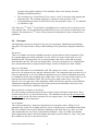
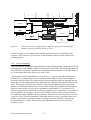
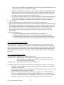
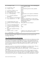
2.1
Parameter Identification Process
Optimisation
p
Model
(ysim)
e(t)
Real System
tested
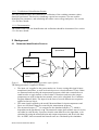
Figure 1.
r(t)
F
SI
(ymeas)
The dynamic fitting procedure (after Spirkl).
The fitting procedure is applied as follows:
• The input e(t) is applied to the system under test. In store testing this signal is input
temperatures and flows, as well as electrical power to electrical heaters. These values
are measured and stored by the measurement program, which also controls the test
stand in order to apply realistic or fixed values. It measures and stores the output
temperatures as well so that the heat transfer rates can be calculated. See Combitest
Program Manual (2000). The input is in the form of several different test sequences
applied to the test object.
• The same signal is applied to the model. Measured data for input temperatures and
flows are read from a data file created by the measurement program.
meas
sim
• The measured output (y ) is compared to the simulated output (y ), which is
dependent on the parameters set p. The measured output, heat transfer rates for stores,
can either be read directly, if present, from the same data file as the input data, or be
calculated by using the measured input and output temperatures and flow in the data
file. At SERC, these measured heat transfer rates are calculated by the simulation
SERC’s Parameter Identification Manual
5
•
•
program using simple equations. The simulated values come directly form the
simulation models themselves.
The deviation (r(t)) is first filtered (F) to remove “noise” in the data, then squared and
integrated (SI). The resulting signal gives a measure of the goodness of fit.
An optimisation procedure is used to derive the best parameter set p – i.e. To minimise
r(t) and hence C(p)
The values for ymeas and ysim can be based on anything but it is usual to have it based on power
(heat transfer rate). For an optimisation problem there is not a real system, and the filter is not
required. The function for ysim can be of any form and is dependent on what is intended to be
opitimised.
2.2
Concepts
The following concepts are integral to the process of parameter identification/optimisation
using DF. For many of them a deeper understanding can be gained by reading the manual for
DF.
Parameters
These are variables used in the simulation model to specify features of the component. They
are constant during the whole simulation. It is the values of certain of these that are to be
identified by DF. In general there are several parameters that can be easily and accurately
determined by the user. DF need not identify these. The more parameters to be identified the,
more measured data that is required and the longer it takes to identify the values reliably.
Objective (Residual)
This is the value that is to be minimised by DF. DF requires two values, or more accurately
time series, the measured value and the calculated value. The comparison between these two is
only one dimensional, so if several different quantities are to be used for optimising they must
be combined with relevant weighting into a single value. This is to be done in the same way for
both measured and calculated values. DF uses not just a single value in fact, it uses the
objective for every time step of the simulation, which can in fact be split into several different
simulations using different measured data. Both measured and calculated values have to be
written out to a file by the simulation program.
Measured Data and Inputs to the Model
For solar heating systems the measured data consists of inlet and outlet temperatures, flows
and electrical power (or if relevant fuel usage). The simulation model uses the measured data
as input values and in effect then calculates its own output values. For a fluid circuit the inputs
are thus flow and inlet temperature.
Local Minima
The results produced by a model are dependent on its parameter values. When several
parameters are varied, the resulting objective can be considered to be a multidimensional field.
DF tries to find the lowest point (absolute minimum) in this field. However, there are often
other minima that are not as low as the absolute minimum – these are called local minima.
Most optimisation routines find local minima and require special routines to “hop” away from
these minima so that new ones can be located.
SERC’s Parameter Identification Manual
6
Cross Correlation Matrix
DF calculates the gradient in the objective with respect to each parameter and file. Information
from this and other changes in the objective from parameter changes are used to derive a cross
correlation matrix where it can clearly be seen how closely parameters are correlated. High
correlation implies it is difficult to identify the absolute values of those parameters accurately
as an increase in one results in a corresponding increase/decrease of the other. With very high
correlations (over 0.95) it can be necessary to fix the value of one parameter and the other be
identified.
Standard Deviation
The variation in identified value for each parameter is multiplied by a weighted factor
dependent on cross correlation with other parameters to get a “Standard deviation” for the
identified value – this is a measure of confidence for the identified value and is given under the
identified value in the results file. Note that it does not represent maximum deviations.
Data files
More than one set of measured data can be used and DF combines the results for each into a
single objective value. These have to be such that the simulation program can read them.
Time Constant
This is used to filter the results in order to remove “noise” in the data due to sensor
uncertainties amongst other things. For a more detailed description read the DF manual.
DDP file
This is a data definition file used by Fittrn. It defines what is unique to a particular data file.
Normally this is just the start, stop, step and data step times. However, it can also include
different starting conditions, or even different components, other parameter values etc as it is
inserted directly into the deck before the deck is run.
Run
A run is a single simulation during the course of the identification process. Up to 50 000 runs
maybe required for large numbers of parameters (up to 20) and files (around 20).
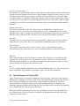
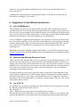
2.3
Special Features of Fittrn and DF
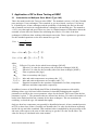
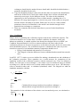
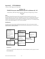
Figure 2 shows how the programs communicate with each other. Fittrn acts as the organiser
initially before handing over control to DF for the actual identification. Fittrn is also used as a
link to Trnsys by modifying the deck before each run and the results after it. The most
powerful features of Fittrn are that it gives a simple graphical interface to choosing and
adjusting parameters and files and also that the user can define what is special to each data file
in a so called DDP file. This gives great flexibility.
DF is itself a DOS program that can cause some problems in certain cases, but usually does
not. With the latest version of Fittrn it is possible to do identifications and still work on the
computer with other tasks.
SERC’s Parameter Identification Manual
7
TRNSYS Deck
DF configuration
Modelimplementation :
Fitting Parameters are
defined with
CONSTANT statements
FITTRN
Initialisation and
Check. Writing the DF
Configuration files
Dynamic Fitting
Program
Deck Modification
Insert actual
parameters and
datafile assiggnements
Modified
TRNSYS Deck
Direct call of the
TRNSYS DLL
New Parameters
New Input data
Formatting and writing
Results
Figure 2.
DF
Call as ext. model
(Parameter, Datafile)
t, yexp(t), ymod (t)
Communication between the programs Trnsys, DF and Fittrn. Figure taken
from Fittrn manual, courtesy of SPF, Rapperswil.
2.3.1 Requirements
The following programs are required:
Trnsys 14.2
Fittrn has not yet been developed for Trnsys 15
DF v2.8 (and above)
This is the only version with minimal parameter steps working properly. DF.exe and RTM.exe
only are required.
Fittrn v2.3
If large numbers of parameters are to be identified together (10 or more) and 20+ local minima
then it is necessary to Windows NT as the operating system.
2.3.2 Limitations
DF allows up to 20 parameters to be identified simultaneously. If more parameters need to be
identified then the process has to be split into different parts.
Windows 95 and 98 cause problems with large numbers of runs. Fittrn crashes after approx.
10000 runs.
DF has reportedly problems with identifying parameters with very different values (orders of
magnitude different). It is therefore necessary sometimes to add multiplication values to the
identified values to give the used parameter values in the model. Type 140 can do this
internally for the relevant values (see section 3.1).
SERC’s Parameter Identification Manual
8
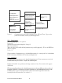
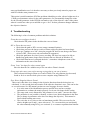
2.4
Alternative Optimisation/Identification Methods
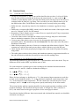
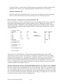
There are many optimisation methods and it is not within the scope of this manual to describe
them all. However, it is worth mentioning two that have been used together with Trnsys or for
optimising solar heating systems.
Multidimensional
Search Algorithms
Gradient
Based
Conjugate
Direction
- O(N2)
DFP
- hessian
- direction
BFGS
- round
off
error
Newton
Pattern
Search
SDM
- inefficient
FletcherReeves
HookeJeeves
NelderMead
+ Conjugate
search
direction
- O(N2)
+ O(N)
+ valleys
- ~O(N2)
+ robust
- dim < ~10
Note:
For calculating the order, it is
assumed that the gradient is
evaluated numerically with
forward or backward differences
+more
- no secant
robust
condition
than DFP + no matrices
Requires line search
All given orders do not contain
the iterations required for the line
search
Efficient for curve fitting
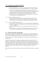
Figure 3.
(modified)
Powell
Some of the many optimisation algorithms available. (From GenOpt 1.0
manual, courtesy of LBNL, Berkeley Univ.)
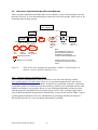
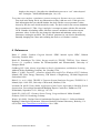
2.4.1 GenOpt (Generic Optimisation Tool)
This is a generic optimisation tool that is available for free from the following website
http://gundog.lbl.gov/GO/index.html. There is very good documentation here and a good
summary of different optimisation methods. GenOpt is not specifically written for a particular
optimisation method or simulation tool instead it has a relatively easy command structure that
handles interfacing to any program. However, four different optimisation routines do come
with the program. GenOpt has been used with Trnsys at ITW, Univ. Stuttgart and at other
sites for both optimisation and parameter identification. It has not been used at SERC. It gives
a good graphical indication of how the identification is proceeding and how the objective
function has become. No cross correlation information is available.
SERC’s Parameter Identification Manual
9
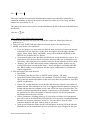
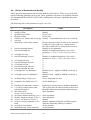
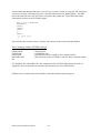
Figure 4.
Interface between GenOpt and the simulation program (From GenOpt
Manual, courtesy of LBNL, Berkeley Univ.).
GenOpt is written in java, which means that this environment has to be installed on the
computer. This is however, free. Because of this GenOpt can be used with virtually any
operating system.
2.4.2 Genetic Algorithm
This is a particular optimisation algorithm that has been implemented in a program at TNO for
optimising large-scale SDHW systems (Loomans and Visser 2000). The search algorithm was
very efficient for this process but has not been implemented in GenOpt or used with Trnsys as
yet. It would thus take some effort to use with Trnsys.
“The standard Genetic Algorithm uses a population (i.e. a group of possible solutions) of
individuals (i.e. parameter sets) that are represented in a binary format. Each parameter is
encoded in a binary string. The strings for the separate parameters then are grouped into one
long string. For the first population, the individuals are randomly determined from the search
space. The ‘fitness’ of the separate solutions is determined subsequently from the fitness
function. The individual that generates the best fitness within the population has the highest
chance to return in the next generation (population of individuals), i.e. reproduction. As
appears in chromosomes in real life, in this new population also recombination is possible at a
given probability. For example, crossover, the exchange of data (in binary format) between
two randomly chosen individuals in the population, and mutation, the transposition of a 0 in a
1 and vice versa. This new generation is calculated and the process is repeated until a given
number of generations is reached or until convergence has been obtained.” Extract from
Loomans and Visser (2000). More details of the algorithm can be found in a book by
Goldberg (1989).
SERC’s Parameter Identification Manual
10
2.5
Simple Comparison of Methods
DF was designed for parameter identification of solar heating systems and has proven to work
efficiently for them. However, the majority of the work has been done with smaller numbers of
free parameters (<10) whereas combistores often require up to 20 or more. It has been
successfully applied. It is slightly slower than the algorithms used in GenOpt but it does give a
cross correlation matrix that can be used to check whether the results are reasonable and
whether it is better to fix a parameter instead of having it free (variable). This decision is
however difficult and requires experience.
SERC’s Parameter Identification Manual
11
3 Application of DF to Store Testing at SERC
3.1
Introduction to Multiport Store Model (Type 140)
This is the model used in the Trnsys work at SERC. The standard version (v1.95) has 5 double
ports and up to 3 heat exchangers. The extended, as yet not released, version (v1.98) has up
to 10 double ports, 4 heat exchangers and the possibility of calculating the flow on the tank
side of natural convection in encapsulated heat exchangers with attached pipe. The manual to
v1.95 is very thorough and good. However, there is a limited amount of information about the
extended version where the method for calculating the effective UA-value of the heat
exchangers is different when working with natural convection. These equations are given here.
For the standard equations see the user manual for type 140.
UA hx =
1
1
1
+
UA pri UA sec
[
&bhx1 , p ⋅ Tp,in − Tp ,out
UA pri = UA 0 ⋅ m
]
b2
⋅ Tpb,3in
&bhx1 ,s ⋅ [Ts ,in − Ts ,out ]b 2 ⋅ Tsb,in3
UA sec = UA 0 ⋅ m
where,
UAhx
UApri
UAseci
&hx, p
m
&hx, s
m
Effective UA-value for the whole heat exchanger [kJ/h.K].
Effective UA-value for the primary side of the heat exchanger [kJ/h.K].
Effective UA-value for the secondary side of the heat exchanger [kJ/h.K].
Flow on primary side [kg/s].
Tp,in/Tp,out
Ts,in/Ts,out
b1,b2,b3
Flow on secondary side [kg/s].
Inlet and outlet temperatures on primary side. [°C].
Inlet and outlet temperatures on secondary side. [°C].
Empirical constants for the equations. Dependencies on flow, temperature
difference and inlet temperature respectively.
In addition, because of the difficulty that DF has in identifying parameters with widely
differing values, type 140 has a built-in function for internally multiplying the supplied
parameters to model to the correct parameter values for the model. This occurs when the last
parameter is given –7. The parameters that are affected are the base UA-values, the number of
nodes in the model and the time constant for the heat exchangers. This can sometimes be
confusing, so check the type 140 manual thoroughly.
Only two heat loss components can generally be identified whereas it is best (standard practice
at ITW) to have three values. Generally one identifies the UA-value for the bottom separately
and for the top and sides combined. This combined value is multiplied by the proportion of the
side area (with respect to the area of sides and top) to get the UA-value for the sides. The
value for the top is calculated in the same manner.
SERC’s Parameter Identification Manual
12
3.2
Practical Guide
3.2.1 Create the New Trnsys Deck
• Format the Data Reader so that it can read the data files that you have. It is best if all the
data files that will be used with this deck have the same format (i.e. same order for the
columns) so that this data reader can read all of them). Have the time step for the data as a
constant (define in SimCtrl), egg Dstep. This is useful if you have different time steps for
the different data files. Check that the data reader works correctly before proceeding.
• Define the start, stop and step times for the simulation as constants, egg Sstart, Sstop,
Sstep.
• Define also a constant called SKIP, which is used to define how much of the output results
are to be ”skipped” by DF. See DF manual.
• Remember to check whether mass or volume flows are required by the Trnsys components
to be used and convert if necessary.
• Create the values used to calculate the relative errors in energy and power and connect
them to simulation summaries. These are defined below.
• Create a sum of the relative errors in power for all connection and connect this to the
special DF printer. This should have the title Printer DF. The first value in the DF printer
should be a constant 0.
• Make all the parameters that are of interest to constants and define them in SimCtrl. These
constants are read by Fittrn and you can choose which of them to use in the DF runs.
• Check that the deck works properly by looking at the results in the DF printer file and by
using online.
• The online plotter and any other printers and simulation summary components should be at
the end of the deck so that they can easily be removed while running Fittrn.
3.2.2 Equations to Use (Defined in prEN 12977-3)
The following equations are given in prEN12977-3 and should be used in the decks. They are
different to those used at SERC up until the start of 2001.
For each connection x (double port or heat exchanger) the calculated and measured heat
transfer rates (Px,c and Px,m) shall be calculated according to:
&⋅ (T − T )
Px ,c = ρ ⋅ C P ⋅ V
x ,i
x ,o ,c
&
Px , m = ρ ⋅ C P ⋅ V ⋅ (Tx ,i − Tx ,o, m )
Where for heat exchanger or double port x, Tx,i is the measured input temperature (used also
as input to the simulation model), Tx,o,c is the calculated (simulated) output temperature and
&is the volume flow rate into the port or heat
Tx,o,m is the measured output temperature. V
exchanger, and C P and ρ are the average heat capacity and density for the heat transfer.
The average density and heat capacity should be for the normal operating conditions of the
port/heat exchanger. This should be 992 kg/m3 and 4.18 kJ/kg.K for water (valid for 1560°C) and values based on the glycol properties for the water/glycol mixture.
From this the absolute difference between measured and calculated heat transfer rate should be
calculated according to:
SERC’s Parameter Identification Manual
13
∆Px = Px ,c − Px , m
This value, and the measured and calculated heat transfer rates should be summed in a
simulation summary so that can be used to calculate the relative errors in energy and heat
transfer rate (see section 3.2.6).
The value to be used as the objective for the identification by DF is the sum of the differences
for all ports:
objective = ∑ ∆Px
x
3.2.3 Steps to Run Fittrn with a New Deck
1. Create a new directory and copy the 4 Fittrn files (cnfgtr.trn, dfstart.bat, fittrn.exe,
gofit.exe) to it.
2. Copy your own Trnlib32.dll and cnfgtr.trn and your deck to the same directory.
3. Modify your deck to run with Fittrn:
• If you are going to use more than one data file then you have to remove the Assign
statement(s) for the data file(s) in the deck, and remove the following constants
(Sstart, Sstop, Sstep, Dstep, and SKIP) - these will be defined individually in the
DDP file for each data file (see below).
• Check that the path to the data files specified in the Assign statement is correct. It is
often best to have the data files in a separate directory under the working directory
called data - this whole directory can then easily be moved when the next fit is done.
• “Remove” the (for DF) unnecessary output components (online, printers etc) by
writing END on its own line before them – Trnsys will ignore everything after this
line. When results are to be checked this line can be commented to re-include the
output components.
4. First time using Fittrn with the deck:
• Start Fittrn.
• Check that Fittrn knows where to find DF (menu options – DF path).
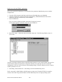
• Open the deck with Fittrn and use the command ”Create DF Config” (bottom right).
This creates the header information at the start of the deck for parameters, data files
and DF configuration.
• Choose DF Config (from the list on the left) and enter the values for the number of
minima and the time constant to be used. It is suggested that 20 minima be chosen as
default and that the time constant is twice that of the time step of the data files. The
number of minima depends on the number of parameters to be identified – the fewer
the parameters the fewer the number of minima required. See the DF manual for
information about the time constant.
• Choose Parameters. Nothing comes up. You now have to add a list of parameters
that will be able to be identified by DF and Fittrn. Use the menu command Edit/Add
Parameter to add new parameters to the list. You can choose from all of the
constants defined in the deck. Add as many as you want.
• Open up the Parameters folder and for each parameter in the list, fill in the allowed
min and max for the identification process as well as the units. Heights for the type
SERC’s Parameter Identification Manual
14
5.
6.
7.
8.
140 store model should use the minimal parameter step option, specifying the size for
a single node (egg. 0.01 if 100 nodes are used).
• If there is more than one data file to be used, then use the menu command Edit/Add
Data File to create a list of these data files. (If you use only one data file, then do not
define a data file in Fittrn - otherwise you have to remove the 5 constants and data
file assign statement in the deck as for multi-file runs.)
• Open up the data files folder and for each data file define a DDP file and put there the
Assign statement(s) for the data file(s) and the following 5 constants (Sstart, Sstop,
Sstep, Dstep, and SKIP), entering the relevant values for each of the constants.
Save the deck!
Choose which parameters and data files that are to be used and mark them.
Specify the start values for the parameters to be identified by creating a new DFP f ile. This
file normally contains the current best parameter set. However, when starting, DF uses the
values as start values, otherwise it uses the minimum values for each parameter. Look at a
previous DFP file for the correct format. The parameters have to be in capital letters,
separated from the value by an equal sign with no spaces. They also have to be in the
correct order.
Start the fitting process.
• Choose which parameters that are initially going to be identified.
• Make initial identification of the store volume and the heat loss coefficients
• Do identifications separately of any circuits where the model is uncertain or new
so that experience can be gained with what parameters are required in the model.
3.2.4 Checks During an Identification
The main thing to check for is whether there is a singular matrix (zero Hesse matrix) and
whether there are very high cross correlations. To get current values press the s key. WAIT
until a menu comes up in the DOS window before choosing the list option (l key). This brings
up the best parameter values and the cross correlation matrix and the identification proceeds
automatically. Note! If you do not wait for the menu to appear and press the s key again, DF
will stop!
3.2.5 After an Identification Run
Two files that DF produces are of interest. They are the:
<filename>.dfr Results file where all information that might be needed is written. See
Appendix B for more details and comments on the example. More details
can also be found in the DF manual.
<filename>.dfp Best fitted parameters from the identification.
The following procedure should be followed after an identification run has been completed.
1. Copy the *.dfr and *.dfp files and give them an appropriate identification tag with the
identification run number.
2. Copy the results at the end of the dfr file into the documentation file for the store being
tested stating what the new files are called.
3. Analyse the results in the dfr file. Are there any very high cross correlations and do
they give very high uncertainties to the identified parameter values? Correlations of
over 0.90 should be looked at more thoroughly. Uncertainties of over 20% for normal
parameters, 0.05 for store heights and 0.2 in exponent values for the internal heat
SERC’s Parameter Identification Manual
15
exchangers should also be analysed in more detail and it should be decided whether a
parameter should be fixed or not.
4. Copy the identified parameter values into the deck that was used for the identification
and run for all files used. Check in the online window how well the calculated and
measured powers agree for the different circuits. The values in the simulation
summaries give also an indication of how well the match is. Anything above 3%
difference in energy input/output for a circuit is not good. If the results are not good
then the model is normally to be blame. Either there are too few of the available
parameters chosen to be identified, or the model is not detailed enough for the
particular heat exchanger or component.
5. Write any comments and decisions about how to proceed in the identification
document.
3.2.6 Verification
Make a deck for simulating the verification sequence and run the verification sequence. The
verification should be two to three days of realistic conditions for summer, winter and
inbetween conditions. A suitable sequence has already been designed for use at SERC (see
Combitest Program Manual). It is best to measure and store the same values for the
verification sequences as for the test sequences, as this allows the same deck to be used as that
in the identification process. The verification sequence is simulated in the same way as the
normal test sequences, but simulation summary components should record:
• Energy, both simulated and measured, for each port.
• Time integral of absolute difference between simulated and measured heat transfer
rates.
In prENV 12977-3 relative errors are defined for making a benchmark test and validation of
the evaluation procedure. These quantities are a useful measure for comparison of the
simulation results of the verification sequence with the measured ones. They are defined as
follows. For each port or heat exchanger, x, the relative error in transferred energy is defined
according to εx,Q and the relative error in mean transferred heat power by εP. The subscript m
refers to measured values and c to calculated (simulated) values. The integrals are what the
simulation summaries calculate.
Qx , c − Qx , m
⋅100%
Qx , m
ε x ,Q =
εP =
∆P
P
where:
Qx,c
Qx,m
⋅ 100%
Calculated heat energy transferred to port/heat exchanger x.
Measured heat energy transferred to port/heat exchanger x.
The quantities for the calculation of the relative error in transferred power, are calculated as
follows:
∆Px = Px ,c − Px , m
SERC’s Parameter Identification Manual
16
∫ ∑ P dt
P=
∑t
x
x
t
x ,t
x
∫ ∑ ∆P dt
∆P =
∑t
x
t
x
x ,t
x
In previous work at SERC, a modified definition of the relative error for transferred power
has been used, εX,P. This is in effect the same measure, but applied to each port/heat
exchanger separately. εP is a measure for all ports combined. The equations used for this are
as follows.
∆Px
⋅ 100%
Px
ε x ,P =
∫ P dt
P=
∑t
x
t
x ,t
t
∫ ∆P dt
∆P =
∑t
x
t
x ,t
t
3.2.7 Guidelines for Determining Whether to Fix a Parameter Value
As stated in section 3.2.5 part 3, it is necessary to look for results that could be unreliable.
Generally correlations above 0.90 and especially above 0.95 are suspect. Also suspect are
uncertainties of over 20% for continuously variable parameters, 0.05 for store heights and 0.2
in exponent values for the internal heat exchangers.
The first step is to check whether the parameters are realistic. This is an engineering
judgement requiring some experience with the method. For the heat exchangers one should
calculate the effective UA-value at potential operating conditions and see how that compares
with results from previous tests and from estimates of what is to be expected. There is a
special Excel sheet for this purpose. Low values of exponents (<0.3) are not generally a
problem, as they do not make the results vary much for typical operating conditions. Higher
values (above 0.8) are much more suspect. If it is unsure whether the result is good or not,
redo the identification for that heat exchanger only with the exponent fixed at 0.0. Check the
results of this not only in online but also in the simulation summaries to check whether the
energy balance for the circuit is under 3%. If it is then use these values.
Heights should be checked against the geometric heights. The geometric height is defined as
the equivalent relative height in the model that has the same volume under it that the real tank
has under the relevant position.
SERC’s Parameter Identification Manual
17
3.2.8 Documentation and Administrative Routines
3.2.8.1 Before the Identification
• Make an excel sheet to calculate the geometric heights of all inlets and outlets
• Prepare the data files to be used in the identification process. Decide what time
step to use for the simulations (and data files). Usually a time step of 0.025 is
used. If there are dynamic effects with shorter time steps that are important for the
model then a shorter time step is required. Document what has been done.
• Prepare the deck for use with Fittrn as described in sections 3.2.1 and 3.2.3.
• Create a directory on the computer where all the identifications are to be made.
One subdirectory for each identification run.
3.2.8.2 During the Identification Process
• Make a document where all the steps of the identification are recorded. This
should include a brief description of the model used for the different circuits. A
short description of each run and the conclusions from them should be made.
3.2.8.3 After the Whole Identification Process
• Create an Excel sheet with the results of the verification sequence and calculate
the relative energy error and relative power error for each port as defined in prEN
12977-3 for validation.
• Copy the parameter values to the Excel sheet with all the values for the stores
tested.
• Write a document describing the best identified parameters and the models used.
See Appendix C. Put a printed copy of this in the file with the other reports.
3.3
Creation of Data files and DDP Files
Data files are created from the measured data files. First it has to be decided what the time
step of the data is going to be. Generally we have used 0.025 hr for both data and simulation
time step. If more detailed dynamic effects are to be studied then a shorter time step is
required. The time step of the measured data has to be the same or shorter than that used in
the simulations.
DDP-files are files that allow customising of simulations dependent on the data file. The
contents of the data file are inserted into the deck before it is run. Generally the contents are
just the start, stop and time step as well as the assign statement for the data file. However, it is
in principal possible to have completely different system for each data file in the DDP-file as
any contents that are Trnsys input commands can be there. Often all that is required above the
normal is reallocation of ports that may be used for different purposes in different test
sequences.
More details of the creation of data files and their associated DDP-files are given in Appendix
A.
SERC’s Parameter Identification Manual
18
3.4
Choice of Parameters to Identify
This is the most important but also the most difficult of the choices. There are no fixed rules,
but the following guidelines can be given. These guidelines will need to get updated with time.
It is intended that IEA SHCP Task 26 Solar Combisystems will create a guideline document
about this.
The following refer to the parameters in type 140 v1.95.
No
1
2
3
4
5
6
7
Description
storage height
storage volume
Specific heat of fluid
Density of fluid
effective vert. therm cond. in storage
not used
initial temp. of the whole system
8
9
heat loss through bottom
heat loss through top
10
11
rel length 1st zone
heat loss through 1st zone
12
13
14
15
16
17
rel. length 2nd zone
heat loss through 2nd zone
rel. length 3rd zone
heat loss through 3rd zone
heat loss through 4th zone
rel. height inlet 1st doubleport
18
rel. height outlet 1st doubleport
19
stratified charge 1st dp? yes=1
Guide
Fix to measured height of cylindrical part of store
Identify
Fixed (4.18)
Fixed (992)
Identify – if time limited then fix to 4.5 kJ/h.m.K
Fixed to measured value for start of test sequence.
Usually 20°C but could vary – maybe need to
have this in DDP file if it varies from test to test.
Identify as own parameter
Identify as combined parameter (UAls1) with
parameter 11, UAlstop = UAls1*Atop/(Atop+Asides)
1
Identify as combined parameter (UAls1) with
parameter 9, UAlstop = UAls1*Asides/(Atop+Asides)
0
0
0
0
0
Identify if used – might be difficult if near top or
bottom
Identify if used – might be difficult if near top or
bottom
Fixed – dependent on store
20- parameters for double ports 2-5
31
32- Positions of temperature sensors 136 5. Used for control sensors and
general information
37 aux heater mode
(0=no,1=Pvar,2=Pconst)
38 aux heater installed from top? yes=1
39 absolute length aux heater (if 38=1)
40 rel. pos. aux heater (if 38 not 1)
41 rel. pos. of temp. controller to aux
heatr
42 set temp. for aux heater
43 dead band temp. of the controller
As for double port 1
Store dependent
Store dependent
Identify
Identify separately using EiA and EiB sequence
when the electrically auxiliary is enabled.
As for param 41.
As for param 41.
SERC’s Parameter Identification Manual
19
Positions for control sensors should be identified.
This is done after the other parameters have been
identified. Match measured and simulated temps.
Store dependent
44
rel. inlet pos. 1st hx
Fixed to geometric height – can try identifying but
it is normally not possible
45 rel. outlet pos. 1st hx
Identify
46 Volume of 1st hx
Fix to estimated equivalent volume (included
metal)
47 specific heat of fluid in 1st hx
Fixed
48 density of fluid in 1st hx
Fixed
49 UA- number from 1st hx ; *1/1000 Identify
50 b1.1 – flow dependency
Identify if there are test sequences with different
flows
51 b1.2 – temperature difference
Fix to 0. Can try identifying with separately but
dependency
usually is 0.0
52 b1.3 – temperature level dependency Identify
53 Time constant for hx 1 * 1 / 1000
Identify if it is thought there is a time constant
associated with the UA-value. Usually only DHW
discharge heat exchangers
54 stratified charging with 1st hx?
Store dependent
55- parameters for heat exchangers 2 & Same guide as for heat exchanger 1
76 3
77 accuracy for calculating temperat.
0.001 or 0.0001
78 accuracy for UA when using b*.*
10
79 precision of mixing process in the
10000
tank
80 flag if temp. dependence timestep
0
control
81 Number of nodes / *1/10000
Usually 0.01 but could be 0.005 or 0.004 or even
0.002 if less accurate model was desired
82 0 = normal mode; -7 = fit mode
-7
For other components a choice will have to be made based on previous experience and
knowledge of the model.
3.4.1 Note on Parameters for Heat Exchangers
The above guidelines are for heat exchangers that are placed in the store without any covering.
They produce mixed charging and discharging. If these are covered (encapsulated) then it is
more accurate to treat them as a counter flow heat exchanger with natural convection on the
store side. They can either be modelled using a separate heat exchanger component (type 5 or
type 105) along with equations to define the natural convection flow, or with v1.98+ and
above of type 140.
In the latter case there are extra parameters for defining how to calculate the flow. These are
defined in the notes on the changes to type 140. Suggested values for these are:
schx = 2 for heat exchangers with stratifier unit (with holes/flaps), -2 for heat exchangers with
simple pipes.
smhx is the flow factor for the natural convection. A positive value is suggested, when the
flow calculation is based on the average store density over the height of the pipe. A negative
value uses the density of the store at the pipe outlet. A test should be performed to see which
one works best for a given device. Sometimes this parameter can be quite high (over 100) in
SERC’s Parameter Identification Manual
20
which case it is suggested that a multiplying factor is used so that the identified value is
between 0 and 10.
In addition the equations used for calculating the effective UA-value are not the same for
enclosed heat exchangers. See section 3.1.
4 Suggestions To Aid Efficient Identification
4.1
Use of RAM Memory
The identification process can use the hard disk repeatedly. This is dependent on how the
operating system is set up and the other programs used on your computer. If you notice that
this is the case for your computer then it might be good to use a RAM disk. This helps in two
ways. One the retrieval of data is much faster. Two the load on the hard disk is much smaller.
Disks have been known to crash with continued use for identification.
A size of 8 Mbytes is suggested, although this is very dependent on the size of the data files
used. The easiest method is to copy the whole working directory to the RAM disk, including
data files and programs (Fittrn.exe, fittrn.ini, gofit.exe, dfstart.bat and trnlib32.dll). The two
parts of DF, DF.exe and RTM.exe can usually be left on the hard disk, as they are not
repeatedly run.
RAM disks can easily be installed on Win95 and Win98, as it is part of the operating system.
For NT a separate program (NTRAMDSK) must be downloaded from the following website
http://www.ntfaq.com.
4.2
Maximum and Minimum Parameter Values
These affect how DF calculates the derivatives (gradients) for the individual parameters. Too
small a value and sometimes DF can have problems in calculating a gradient, in which case a
singular matrix will result. On the other hand a too large value can result in crashes or system
instability (for certain models). Care has also to be taken with heights for inlets and outlets as
if the values are too large, then it is possible to get heat exchangers 2 and 3 overlapping –
something not allowed in the model.
Generally speaking it is best to give quite large ranges of the order of one magnitude. If the
value cannot be estimated, then a wider range is required. Exponents for the heat exchangers
should be in the range 0-1 but a range for the identification of 0-2 is suggested. Parameters
that influence the results significantly can usually have smaller ranges. These are often certain
inlets/outlets and the volume.
4.3
Use of DF /Q
It is possible to get an objective function value for the model for a given parameter set using
the following command in the DOS window:
DF <filename> /Q
where <filename> is the name of the deck but without the extension.
DF takes the values in the DFP file for use in the calculation. A DF file is also required. This
defines which data files to use and the ranges for the parameters and is created when Fittrn
SERC’s Parameter Identification Manual
21
starts an identification run. It is therefore necessary to have previously started a proper run
with DF with the same parameter set.
This option is useful sometimes if DF has problems identifying a value, often a height near 0 or
1. With good parameter values for the other parameters, one can manually change the value
for the relevant parameter in the DFP file and make a note of the objective value. Other times
when it is useful are when you would like to get a “feel” for how parameter changes influence
the objective function.
5 Troubleshooting
The following is a list of common problems and their solutions.
Fittrn does not configure the deck
Check that the DF printer in the deck has the correct format.
DF or Fittrn does not work
• Check that the path to DF is correct (menu command Options).
• Check that you have the latest version of Fittrn (older ones have had some bugs).
• If you get ”runtime error 200” when the program DF itself is run, then get the latest
version of DF. (This occurs only on Pentium II computers).
• Check the path name for where you are working. DF does not seem to be able to
handle long path names (longer than 8 letters) that are allowed in Windows 95.
• Check that fittrn has not corrupted the deck – sometimes it duplicates some of the
information at the start of the deck.
Fittrn ”loses” the data files when started again
Have the data files in a subdirectory to the one where Fittrn is located.
Fittrn stops after many runs with a message saying that its run out of memory
This is an unsolved bug in Fittrn (as of end of 2000). The only solution (work around)
found so far is to run the whole process on a computer using Windows NT.
Zero Hesse (Singular) Matrix Found
This occurs when there is no change in the objective function when the derivatives are
calculated, i.e. the second derivative matrix of the objective function is zero. This can be due
to several reasons. See DF manual (section on error messages for more details).
• It is at the start of the identification process and DF does not have enough
information to evaluate the matrix properly. Let it run a bit longer before acting.
• The range (min- max) allocated for the parameter is too small - increase the range.
• The parameter is not possible to identify, as there is too little information in the data
files (a change in parameter value does not change the objective). This cannot be
fixed without making more tests.
• The real value is very close to the real maximum possible. This can occur for the
relative heights near 0 and 1, more often near 1. To overcome this you can identify
the value manually using DF /Q (see section 4.3) or construct equations that limit the
SERC’s Parameter Identification Manual
22
height to the range 0-1 but allow the identification process to “use” values beyond
this. Useheight = MAX(MIN(identheight, 1.0), 0.0)
Trnsys does not complete a simulation (various messages in German can occur with this)
First look in the listing file for any information on why it did not work. If this gives too
little information then you should simulate the deck with the correct parameter values
chosen by DF (the ones which caused the crash). The deck used for the current simulation
has an extension of *.TRA. Copy it and give it a temporary name with the file extension
.DCK. Simulate it including online. Often the system is unstable with certain extreme
parameter values. In this case just change the maximum and minimum values of the
parameters causing the problem. The “problem” parameter(s) can often be identified by
manually changing the values and rerunning the deck to see whether it crashes.
6 References
Bales, C. (2000). Combitst Program Manual. SERC internal report, SERC, Dalarna
University, Sweden, 2000.
Drück H., Pauschinger Th. (1996). Storage model for TRNSYS, TYPE140, Users Manual,
Version 1.0 (+updates). Institut für Thermodynamik und Wärmetechnik, University of
Stuttgart.Drück.
Goldberg, D.E. 1989. Genetic Algorithms in Search, Optimization, and Machine Learning,
Addison-Wesley Publishing Company, Inc., Reading, USA.
Hüber, C (1998). Fittrn/DF – parameter identification with DF for Windows 95/NT. Software
Manual. SPF Solar Energy Laboratory, ITR School of Engineering, CH-8640 Rapperswil,
Switzerland 1998.
Klein S. A., et al. (1996). TRNSYS A Transient System Simulation Program, TRNSYS V14.2.
Manual, Sept. 1996. SEL, University of Wisconsin, Madison, USA.
Loomans, M and H. Visser (2000). Application of the Genetic Algortihm for Building System
Optimisation. Proceedings International Building Physics Conference, Eindhoven, The
Netherlands, September 18-21, 2000, pp. 107-114.
Spirkl, W. (1995). DF - Dynamic System Testing, Program Manual. InSitu Scientific
Software, D-82110 Germering, Germany.
Wetter, M. (2000). GenOpt Generic Optimization Program Version 1.1. Software Manual.
Building Technologies Department, Lawrence Berkeley National Laboratory, Berkeley, CA
94720 USA. http://simulationresearch.lbl.gov. Nov. 2000.
SERC’s Parameter Identification Manual
23
Appendix A Making Trnsys Data Reader Files From Measured Data
A.1 The program CTS
CTS is a program developed by SPF in Switzerland. It can average the raw data to equal
length time steps. The following is the way it should be used with the measured data from
SERC.
A.2 Format of Trnsys Data Files
These are the files read in by Trnsys – one for each test sequence. First decide what the format
of the data files is to be. All data files including the verification sequence should have the same
structure (i.e. same columns) in order to be able to use the same data reader in all cases. The
alternative to this is to have several different data readers and therefore decks for identifying
parameters.
Things to watch out for:
• the measured boiler flow (Vb) is used both for full charge (Vfc) and for the boiler
(Vob) in the Presim model and deck. There are no test sequences where both Vfc and
Vob are used. To deal with this you can either:
o Use a switch in the DDP file to say whether the Vb is for Vfc of Vob in this
data, egg Vfcon = 1 (for full charge tests and Vfcon = 0 for oil boiler tests) in
the DDP file, and in the equations calculating the mass flows in the main deck,
Vob = (1-Vfcon)*Vb and Vfc = Vb*Vfcon. Preferable option.
o create two separate columns in the data files and manually copy the Vb to the
Vob column for the few tests where the boiler ports are used
o Identify the boiler ports separately using different decks.
• If you have more than 18 columns in the Trnsys data file (including the time column),
then 2 data readers are required. These need not be the same as each other, rather can
be created separately from Excel (see below).
A.3 Creation of the Trnsys Data Files
A.3.1 Removing Unwanted Data
•
•
•
•
•
•
Load a measurement data file into Excel – make sure that the column titles are ok
using the text import guide.
Remove the columns that are not to be used in the Trnsys data files. Generally these
are Ts1-7, Tbc, Tcc, Tc, Thc and often Tcxi.
Remove the comment lines at the bottom of the measured file with all the energy
balance information.
Remove the top two rows (lines) of the file leaving just the column titles and the data.
Remove bad data points. These are denoted as –9.99. This is normally only for flows.
Use the replace function (CTRL+H) and replace –9.99 with a relevant value based on
the values before and after – often 0.
Regularly the measured flow is 0.001 to 0.005 due to extra pulses coming into the flow
sensors. These make no difference to the energy balance but can be a nuisance in the
Trnsys simulations. If you have time it is worth editing these to zero – using the
replace function (CTRL+H) changing 0.005 to 0, 0.004 to 0 etc. NOTE – do not
change all values at once as this might change some of the time values!
SERC’s Parameter Identification Manual
24
A.3.2 Splitting into separate test sequences
•
•
Create separate excel books for each test sequence by copying sections from the
measurement data file. These can be found by seeing where the flow in conditioning
(Vdx) changes from 0 to non-zero. Each test sequence should start with roughly 0.05
hr of conditioning. The end of the test sequence can be when the outlet from the store
has gone below 20.5°C if the test sequence is going to be used separately. If the test
sequence is to be joined to another test sequence to form a larger data file than the
whole conditioning period is required.
Save each test sequence file as a TAB separated file with the relevant test sequence
name and extension of .tab.
A.3.3 Creating the Trnsys data files with CTS
•
•
•
•
•
Start CTS
Load an existing configuration file (.CFG) and save it with a suitable name for the
store being tested. This file should be nearly the same as that used for previous stores,
except possibly for the flow coupling (see below).
Edit the CFG file. The only thing to check is the flow links. This links temperature
sensors to flow sensors so that the temperatures calculated for longer time steps give
the correct energy output. If the flow is zero then the flow-linked temperatures in the
output file will also be zero. Tci&Tco linked to Vc, Tbi&Tbo to Vb,
Tdhwi&Tdhwo&Tdhw1&Tdhwt to Vdhw. Thi and Tho should NOT be linked to Vh
or to Vdx as they are used with both these flows.
The following are the standard settings to be used in the CFG file (in the order going
down):
ƒ Inoptions: Tab, 1, tbHour, Header exist, special data offset yes – 1.
ƒ OutOptions: no header, no automatic…, Tab, ffFixed, 6,3,dfd.
ƒ CTSOptions: 0.025, tbHour, smNextFit.
Convert the test sequence data files. Note that it is possible to append files together to
create a longer file – this could be useful to reduce the number of files, but implies that
the individual test sequences in the larger file always get run together.
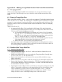
A.3.4 Create the DDP files for each Trnsys data file
This should have the form shown in the example below. Note that in the data reader in Trnsys,
the first parameter should be set to 2 so that the first data line is for the start of the simulation.
CONSTANTS 6
Sstart = 16.525 * Sstart is the start for the simulation – the same value as the first time in the data file
* Sstop is end of simulation – should be two time steps less than the time at the end of
Sstop = 8.35
the measurement data file
* Sstep is Trnsys simulation time step – should be same as Dstep
Sstep = 0.025
Dstep = 0.025 * Dstep is the time step for the data file – set in CTS – usually 0.025
* skip is time to skip at start of data file – always 0.
SKIP = 0.0
* Vfcon controls whether the flow Vb is for full charge (Vfcon=1)
Vfcon = 1
or for oil boiler (Vfcon=0).
ASSIGN data\CIS-sl2.dfd 21 * name of the data file normally in subdirectory data.
SERC’s Parameter Identification Manual
25
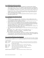
Appendix B Example DF Results File
This appendix gives an example DF results file (*.dfr) and describes the various sections and
gives comments on the results shown.
The start of the file lists the basic identification constraints for DF for the identification such
as parameters, max/min values, and data files.
*** DF 2.7 Oct 97 @Copyright InSitu running 31.05.1999 08:05:12
> TimeBase,1
> FilterConst,1
> Precision,1.0
> TimeBase,3600
> FileName,F:\c500c2\c500all1
> Model,Extprog,GOFIT.EXE
> Model,Dimension,4
> Model,OutputUnits,> Model,ParSpec,1,DHXUA,KJ/HK
> Model,ParSpec,2,DHXB1,> Model,ParSpec,3,DHXB3,> Model,ParSpec,4,DSMDOT,> Model,Range,1, 1.00000000000000E-0001, 2.00000000000000E+0002
> Model,Range,2, 0.00000000000000E+0000, 2.00000000000000E+0000
> Model,Range,3, 0.00000000000000E+0000, 2.00000000000000E+0000
> Model,Range,4, 1.00000000000000E+0000, 5.00000000000000E+0002
> Read,C5PT01\DHW-HF.DAT,Skip=0.000000
> Read,C5PT01\DHW-HIF.DAT,Skip=0.000000
> Read,C5PT01\DHW-HIP.DAT,Skip=0.000000
> Read,C5PT01\DHW-HP.DAT,Skip=0.000000
> Read,C5PT01\DHW-LF.DAT,Skip=0.000000
> Read,C5PT01\DHW-LP.DAT,Skip=0.000000
> FilterConst, 2.00000000000000E-0002
> NumOfLocMin,20
> Fit
Reading parameters from file F:\C500C2\C500ALL1.DFP
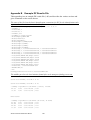
The middle part lists the local minima found after each attempt at finding a new one.
Search local minimum, trial No 1 of 20
Search local minimum, trial No 2 of 20
Search local minimum, trial No 3 of 20
* summary of potential local minima (3 trials, 2 found)
42.669
0.728
0.000 145.801 | 1982
65.919
1.023
0.000 159.768 | 2333
Final search
* summary of potential local minima (20 trials, 18 found)
41.783
0.726
0.000 150.375 | 1971
42.334
0.735
0.000 150.371 | 1971
42.017
0.730
0.000 149.865 | 1971
39.361
0.722
0.015 150.537 | 1973
SERC’s Parameter Identification Manual
26
43.073
0.741
0.000 147.938 | 1974
44.034
0.753
0.000 146.801 | 1978
42.669
0.728
0.000 145.801 | 1982
49.748
0.834
0.000 149.565 | 2005
12.281
0.708
0.424 149.617 | 2023
51.102
0.838
0.000 143.357 | 2023
11.870
0.689
0.425 150.506 | 2024
23.219
0.667
0.159 161.993 | 2026
53.938
0.894
0.000 155.894 | 2087
1.822
0.769
1.270 150.472 | 2128
1.026
0.694
1.476 157.356 | 2157
65.919
1.023
0.000 159.768 | 2333
108.014
1.261
0.000 136.928 | 2879
91.301
1.223
0.000 163.186 | 2897
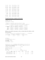
The final section gives a summary of the results.
\NumOfData,432
\NumOfDataCorr,427
\SumTime,109476[s]
\SpectralError,9.96E8[s]
* analysis of variability and intercorrelation of data
\EigenValues of normalized Hesse Hn[i,j]=H[i,j]/Sqrt(H[i,i]*H[j,j])
3.376410030
0.593126404
0.029943105
0.000520461
\EigenVectors of Hn (each column one eigenvector)
DHXUA
0.536077606 -0.204063538
DHXB1 -0.527858381
DHXB3
DSMDOT
0.258481754
0.536088516 -0.200425221
0.382877831
0.397195619
0.716389917
0.808792107
0.020199999
0.431350264 -0.697406470
0.922699835 -0.045032399
0.001289568
Measure of variability of parameter values with and without the influence of the
intercorrelation
\ErrorNoCorr (parameter error ignoring intercorrelation, = 1 / variability)
0.3866
0.00589
0.003069
1.793
\ErrFactorCorr (error increase/factor due to intercorrelation)
31.49
4.778
30.67
1.245
\Parameters
Param,DHXUA,KJ/HK,0.1,200,0
Param,DHXB1,-,0,2,0
Param,DHXB3,-,0,2,0
Param,DSMDOT,-,1,500,0
\Results DF 2.7 Oct 97 @Copyright InSitu running 31.05.1999 10:37:30
\Value,Parameters,"DHXUA=42 DHXB1=0.729 DHXB3=0 DSMDOT=150 Obj=1970"
* External model GOFIT.EXE
frequency transform method............... Cosine
initial state value...................... 0
numerical precision...................... 1
time base................................ 3600
filter type.............................. Gaussian, tf=0.02
Name
mode
tvf
t_start
t_skip
t_end
N*
Size
C5PT01\DHW-HF.DAT
Mean
1
0
0
6.1
86.5
1..610
C5PT01\DHW-HIF.DAT
Mean
1
0
0
5.45
77.4
1..545
C5PT01\DHW-HIP.DAT
Mean
1
0
0
4.13
58.8
1..413
SERC’s Parameter Identification Manual
27
C5PT01\DHW-HP.DAT
Mean
1
0
0
3.53
50.3
1..353
C5PT01\DHW-LF.DAT
Mean
1
0
0
6.46
91.6
1..646
C5PT01\DHW-LP.DAT
Mean
1
0
0
4.74
67.4
1..474
DHXUA
DHXB1
DHXB3
DSMDOT
objective
[KJ/HK]
[-]
[-]
[-]
[-]
41.65
0.7247
2.508E-4
150.3
1971.3
11.8
0.0276
0.0913
2.21
The above line gives a measure of uncertainty of the result (absolute value), including the
effects of intercorrelation – a standard deviation value.
Cross correlation matrix:
1.0000000
0.2368541 -0.9874529
0.2368541
1.0000000 -0.0856613 -0.1383960
-0.9874529 -0.0856613
0.0258676
1.0000000 -0.0720066
0.0258676 -0.1383960 -0.0720066
1.0000000
Note that in this example the cross correlation matrix shows very high correlation between the
base UA-value (DhxUA and the temperature exponent b3). This is quite common but in this
case it causes a very high uncertainty for these two values. In this case the identification
should be redone with b3 fixed to 0.
SERC’s Parameter Identification Manual
28
Appendix C Example Identification Report – SERC2
Model Parameters for Type 140, Multiport Type 140, v1.98F
Chris Bales
SERC. 990615
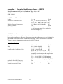
C.1 General Parameters
Height:
Heat Loss Coefficient: CEN
1.42 m
{fixed}
UAs1 = 1.89 W/K (6.80 kJ/h.K) {fit}
UAbot = 0.41 W/K (1.48 kJ/h.K) {fit}
1.28 W/m.K (4.62 kJ/h.m.K)
{fit}
100
{fixed}
465 litres
{fit}
(+ 10 litres water and 1 litre antifreeze
in heat exchangers.)
Effective Vertical Conduction:
Number of nodes
Water Volume
C.2 Collector Loop
The collector loop was modelled using an internal heat exchanger with natural convection
based on the temperature difference between average tank temperature over the height of the
pipe and the outlet temperature from the heat exchanger. Perfect stratification is assumed.
Tests were made using antifreeze mixture with 41% P44 glycol.
C.2.1 Heat Exchanger
Volume
Inlet
Outlet
Heat Transfer Coefficient (UA)
1 litre antifreeze
{fixed}
0.83 [relative height]
{fit}
0.04 [relative height]
{fit}
UAh1 = 1096 kJ/h.K
{fit}
bh1=0.738, bh2=0.0, bh3=0.726 {fit}
UA is dependent on both the primary and
secondary conditions (and thus temperature
distribution in the store).
UA = 190-360 W/K @ 3 kW charging
UA = 250-420 W/K @ 6 kW charging
(UA-value calculated using log. temp. diff.)
On
Average tank temperature over heat exch.
59.1
{fit}
Option for Stratified Charging
Natural Convection Mode
Natural Convection Factor
SERC’s Parameter Identification Manual
29
C.3 Boiler Heat Exchanger
This was modelled as an internal heat exchanger. It operates at high flows (600 l/h or more).
Volume
4 litres water
{fixed}
Inlet
0.80 [relative height]
{fixed}
Outlet
0.43 [relative height]
{fit}
Heat Transfer Coefficient (UA)
UAh1 = 7.77 kJ/h.K
{fit}
{fixed}
bh1=0.0, bh2=0.0
bh3=1.510
{fit}
This gives a UA-value at Tm=70°C
and flow of 600 l/h:
UA70,600 = 1315 W/K (4736 kJ/h.K)
Option for Stratified Charging
Off
Natural Convection Mode
None
C.4 Heating System Heat Exchanger
This was modelled as an encapsulated internal heat exchanger. It operates at low flows (<120
l/h).
Volume
4 litres water
{fixed}
Inlet
0.42 [relative height]
{fit}
Outlet
0.81 [relative height]
{fit}
Heat Transfer Coefficient (UA)
UAh1 = 38590 kJ/h.K
{fit}
bh2=0.0
{fixed}
{fit}
bh1=0.946, bh3=0.0
This value is dependent on both primary
and secondary flows.
Option for Stratified Charging
Off
Natural Convection Mode
Average tank temperature over heat exch.
Natural Convection Factor
60.2
{fit}
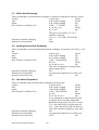
C.5 Hot Water Preparation
This was modelled using an internal heat exchanger with down pipe.
Volume
2.4 litres water
{fixed}
Inlet
0.00 [relative height]
{fixed}
Outlet
1.00 [relative height]
{fixed}
Heat Transfer Coefficient (UA)
UAh1 = 42670 kJ/h.K
{fit}
bh2=0.0
{fixed}
bh1=0.726, bh3=0.0
{fit}
UA is dependent on both the primary and
secondary flows (and thus temperature
distribution in the store). For 60°C in store.
UA = 800-1400 W/K @ 300 l/h draw off
UA = 1900-2500 W/K @ 900 l/h draw off
(UA-value calculated using log. temp. diff.)
Option for Stratified Charging
Off
Natural Convection Mode
Average tank temperature over heat exch.
Natural Convection Factor
145.8
{fit}
SERC’s Parameter Identification Manual
30
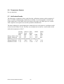
C.6 Temperature Sensors
Not yet identified.
C.7 Verification Results
The following is a summary of the results from the verification sequence which comprised 3
days of realistic conditions and a fourth day of standby. It was not possible to measure the
outlet temperature of the DHW before the mixing valve and so the DHW port was verified
with a separate test sequence not used for parameter identification.
The heat exchanger for space heating was connected as in a real system as a preheater on the
return from the radiator circuit. The flow was calculated to be that for a circuit with a boiler
with outlet temperature of 80°C.
Heating Collector Final
DHW
Boiler
System Loop
Disch.
Port
kWh
kWh
kWh
kWh
kWh
Energy Totals- meas -31.8
22.8
-11.8
-28.8
47.8
Energy Totals-sim -32.6
21.5
-12.9
-28.3
48.4
Differences between measured and simulated according to CEN.
Energy Difference 2.5%
-5.6%
9.4%
-1.7%
1.2%
Mean Power Diff. 7.3%
17.7%
13.4%
1.7%
6.3%
SERC’s Parameter Identification Manual
31
C.8 Schematic of Tank
Bi/SHo
Bo/SHi
DHW
CW
Si
So
T b1
T b2
Ci/FCo
Co/FCi
SERC’s Parameter Identification Manual
T cc
32
Appendix D
FITTRN MANUAL
Courtesy of SPF, Rapperswil, Switzerland.
FITTRN / DF
TRNSYS Parameter identification with DF for Windows 95 / NT
Christof Huber, SPF Solar Energy Laboratory, ITR School of Engineering, CH-8640
Rapperswil
6.3.98
Intro
The Parameter identification program DF from Scientific Software, Munich is used by several
Institutes within their solar collector test and SDHW test activities. DF is a DOS program which calls
external model implementations trough a textfile based interface. This article describes the program
FITTRN, which enables the parameter identification of TRNSYS models by DF. An advantage thereby
is the use of the efficient Windows 95 / NT version of TRNSYS.
Architecture
The diagram shows the parameter identification information flow. The user only needs to call the
FITTRN program. The DF configuration, thus the specification of the parameters as well as the used
input data files are defined in the deck.
TRNSYS Deck
DF configuration
Modelimplementation :
Fitting Parameters are
defined with
CONSTANT statements
FITTRN
Initialisation and
Check. Writing the DF
Configuration files
Dynamic Fitting
Program
Deck Modification
Insert actual
parameters and
datafile assiggnements
-
DF
Modified
TRNSYS Deck
Direct call of the
TRNSYS DLL
New Parameters
New Input data
Formatting and writing
Results
Call as ext. model
(Parameter, Datafile)
t, yexp(t), ymod (t)
Initialisation:
The deck is read and the DF configuration file is written. Subsequently, the DF program is started.
-
Deck modification :
SERC’s Parameter Identification Manual
33
DF calls FITTRN as external model. FITTRN modifies the original deck with the parameters and
input data of the current Fit run. Dependent-dependent TRNSYS blocks are also inserted.
-
TRNSYS Simulation Call:
FITTRN calls directly the TRNLIB32 DLL. After the end of the TRNSYS simulation the output
data are written on the DF format. The control of the process is transferred back to DF.
Deck extensions recommended to run with FITTRN / DF
The DF configuration is written as comment block directly into the TRNSYS deck. Some conventions
must be kept. The configuration block is marked with the keywords ”BEGIN DF CONFIG” and
”END DF CONFIG”. This Block is automatically written by the FITTRN program. Changes
of the configuration should be made trough FITTRN. The following paragraph shows a typical
configuration block.
** BEGIN DF CONFIG
* PARAMETER
MIN
* CAP
0.1
* C0
0.7
* C1
10
* CPA2
0.05
* IAM
0.2
* VOL
0.0002
* DATA FILE
* DATA\DATA01.DAT
* DATA\DATA02.DAT
*
* FILTERCONST = 0.1
* NUMOFLOCMIN = 20
*
* DATA DEPENDENT BLOCK
MAX
5
0.9
20
10
0.5
0.005
UNIT
KJ/K/M2
KJ/H/K/M2
0.01KJ/H/K2/M2
-
SWITCH
OFF
ON
ON
ON
OFF
OFF
SWITCH
ON
ON
MINSTEP
OFF
OFF
OFF
OFF
OFF
OFF
** END DF CONFIG
After the keyword " PARAMETER " follows the listing of the parameter names, their certified
variation area as well as a switch. This switch serves switching a Fit parameter on and off, without
deleting equal the appropriate line. The parameters are defined in the deck by normal CONSTANTS
statements. FITTRN detects these definitions and exchanges the values during the identification
process. The keyword DATA FILE marks the data files used for the identification. Also here a switch
can be set. In the further two DF configuration instructions, the time constant for the low-pass filter as
well as the number of local Minima can be set.
The lines between the keyword ”DATA DEPENDENT BLOCK” are used to insert TRNSYS
statements which depends on the specified data file. This statements must be defined in a text file which
has the same name as the corresponding data file but with extension ”.DDP” The convention for this
file is the ASSIGN statement of the data file and the Constant SKIP which are needed for each data
file. The simulation times also must be defined in this file. At each TRNSYS run, the lines of the DDP
file are copied and inserted in the deck. This enables full flexibility for example the use of more than
one physical data file as input or data file dependent Units.
SERC’s Parameter Identification Manual
34
The measured and simulated functions ymod(t) and yexp(t) must be written to a text file. The convention
you have to look for is that the printer unit is marked with the keyword „PRINTER DF”. FITTRN
detects this and reads the result file which is assigned to this printer unit. This modification is not
automatically inserted by the FITTRN program.
UNIT 53 TYPE 25 Printer DF
PARAMETERS 4
STIMEST
SIMSTART
SIMEND
46
INPUTS 3
0,0
Pmeas
Pcalc
0.
0.
0.
The result file must contain at least 3 columns. The columns are described in the DF Manual.
Files coming up with the FITTRN package
FITTRN.EXE
FITTRN.INI
GOFIT.EXE
DFSTART.BAT
DF.
: Main program
: Configuration File
: DOS Interface which is called by DF as external model.
: DOS batch file used by FITTRN to start DF. Must contain the path to
The TRNSYS DLL TRNLIB32.DLL the configuration File CNFGTR.TRN and the deck file are
supplied by the user and need to be located in the same directory as the FITTRN files.
FITTRN can be obtained from Christof Huber, email [email protected]
SERC’s Parameter Identification Manual
35
Quick start with the DEMO Application
These steps explain the installation of FITTRN and a first parameter identification process with the
example deck.
1. Copy the 4 Files located on the Disk in the directory \PROGRAM on your Harddisk.
2. Copy the example files located on the Disk in the directory \PROGRAM inclusive the DATA
subdirectory into the same directory on the Harddisk.
3. Start FITTRN.EXE
First, we need to configure the Path, where the DF program is located.
Choose Menu Options->DF Path.. Insert the correct Path here.
4. Menu File->Open... Choose the demo deck called ”demo.trd”. The following Window comes on
your screen :
You have just loaded a TRNSYS Deck with all needed extensions to work with FITTRN. Now the Tree
on the left side contains the parameters configured to identify, the used Input data files and the DF
configuration. Click on a icon to show the corresponding settings. The Box with the red cross is used to
switch a parameter on or off.
5. Start fitting. Choose Menu File-> Start fitting to start the identification process.
If all is successful, a DOS Window with DF appears on the screen. Then the FITTRN is started for
each run. The FAST! flag on this Window sets the TRNSYS process to a high operating system
SERC’s Parameter Identification Manual
36
priority. Thus it is not possible to identify in the Background. On Windows NT it is possible that the
mouse is not yet responding until the parameter identification Process is terminated.
To terminate FITTRN you have to terminate DF with typing ”escape” on the DOS Window. !
Steps to modify a deck to run with FITTRN
1. Create a new subdirectory and copy the 4 FITTRN files to it.
2. Copy your TRNLIB32.DLL, CNFGTR.TRN and your deck to this directory.
3. Modify your Deck : Insert the Residual File Printer and mark it with the keyword ”DF PRINTER”
If you use more than one data file, set the SIMULATION times to variables, which you can defin
in the DDP.
4. Start FITTRN.EXE
5. When no DF configuration is found in the Deck, you can create a new configuration. Then you can
add data files and Parameters trough Edit Menu. Set up the DF configuration too.
6. Save the Deck
7. Start fitting
SERC’s Parameter Identification Manual
37