Download 4ep.1.1 how well do pv modelling

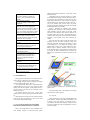
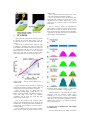
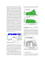
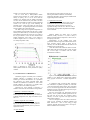
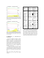
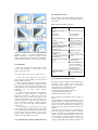
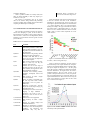
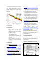
4EP.1.1 HOW WELL DO PV MODELLING ALGORITHMS REALLY PREDICT PERFORMANCE ?
Steve Ransome
BP Solar UK
Chertsey Road, Sunbury on Thames, TW16 7XA UK
Tel: +44 (0)1932 775711 [email protected]
ABSTRACT:
•
•
•
•
•
•
Grid connect PV Sizing programs predict annual energy output in kWh of arrays of solar modules. These are at
specified locations and array orientations; using databases of weather, module and inverter performance with user
defined values for dirt, mismatch, wiring losses etc.
The programs will usually predict performance ratios of 75-80% (approximately what will be achieved in real
measurements).
This paper looks to see if the programs model everything correctly, or if are there sufficient unknowns and user
defined inputs so that predictions and output happen by chance to coincide to within a few percent.
Some differences were found between measurements and predictions from commercial modelling programs
including both the distribution of insolation and the performance of solar modules vs. irradiance.
This paper compares and contrasts algorithms and assumptions used in several commercially available Sizing
programs with real outdoor logged data predominantly from ISET Kassel, Germany and BP Solar’s factory roof in
Sydney, Australia.
It concludes that whereas Sizing programs may use the best available algorithms to help to minimise avoidable
losses due to poor component selection, shading, thermal problems etc. the inaccuracies in the kWh predictions due
to unknowns such as actual/nominal Pmax, actual weather data and dirt/shading losses mean the absolute values
cannot be taken as accurate to within ~5%.
Keywords: Modelling, Simulation, Performance
1) INTRODUCTION
BP Solar have been involved in long term outdoor
PV performance studies of BP Solar’s and competitors’
products since 1998 with IV swept, maximum power
point tracked or grid connected modules and arrays at
many sites worldwide plus a wide variety of cell
technologies. [1]
Models have been developed with these data to
characterise the performance under the wide variety of
weather conditions. Large ac arrays using similar
modules have been logged to see how they actually
performed and compared with the dc data. [2][3]
Some of the modelling in commercially available
sizing programs has been found to differ from real
outdoor measurements (for example both the distribution
of insolation vs irradiance and the PV module efficiency
vs irradiance) or are absent (e.g. modelling spectral
response particularly for multi junction devices or the
thermal and voltage dependency of inverters) yet
predictions of kWh/kWp are routinely quoted to 4-5
significant figures despite uncertainties with some of
these critical yield determining input parameters that can
be of the order of a percent or more each.
While commercial sizing programs are very useful in
helping to design systems to minimise losses (e.g. by
matching optimal inverter power to PV arrays,
calculating thermal properties of roof mounting and the
effect of any shading obstructions), their estimated
kWh/kWp values are imprecise due to the uncertainty of
some of the inputs and differences seen between
modelled and measured performance.
This paper only discusses grid connect sizing programs
(it does not talk about battery storage, pump or hybrid
inputs including wind and diesel) but details of the plane
of array calculations and PV performance algorithms can
be considered in these types of systems.
Definitions of some of the terms used are in appendix A.
2) SIZING PROGRAM METHODOLOGY
Most PV sizing programs predict kWh/year energy
output by using a methodology similar to the following
list:-
Input site data :
site location (latitude, longitude and
elevation) , array orientation (tilt and
azimuth)
Input component type data:
types of PV modules, inverters, BOS
components.
Choice of component numbers :
Guide the user to choose appropriate
component numbers such that the values of
ratios such as “inverter power”/“module
power” are optimal. Check also for voltage
limits for PV strings feeding the inverter.
Get meteorological data :
(horizontal plane insolation, ambient
temperature and wind speeds), interpolate
from nearby sites if necessary.
Divide the year into (usually hourly)
intervals
Predict weather parameters :
(from transition matrices) for each time
period on the horizontal plane:
Estimate weather parameters (from
transition matrices) for each time period on
the module tilted plane
Using details of the mounting type (e.g.
roof integrated, free ventilation etc).
Calculate module temperature (from
irradiance, windspeed and ambient
temperature).
Estimate the module dc Pmax under these
conditions
Calculate the inverter output:
Note the model should calculate for turn
on, clipping and if the Vmax of the
modules is outside Vmpp inverter window.
Sum the predicted ac output power over a
year to give energy yield
radiation and ambient temperature (i) and these will be
discussed further.
Algorithms based on transition matrices [7] (which
store likelihoods of changes between sequential values –
for example if one measurement is sunny there may be a
higher chance that the next will be sunny too) generate
pseudo random series of data with the same sum over a
year as the monthly data, plus the ranges, day-to-day
persistence and other statistical parameters which should
be indistinguishable from real data.
Figure 1 illustrates the different solar radiation
components that contribute to the horizontal and tilted
plane irradiances with the equator to the right. Under
clear skies most radiation comes directly from the sun
with little scatter off a blue sky; whereas under haze or
cloud the beam component is lowered and most radiation
impinging on the module comes from scattering off
clouds.
Note that tilting the plane towards the equator will
normally increase the beam component, add some
reflection component and decrease the diffuse (as some
of the diffuse sky is now behind the module). Often
quoted statistics such as “x% of the insolation at a site is
diffuse” where x = Diffuse / (Diffuse + Direct) only refer
to the horizontal plane. When modules are tilted towards
the equator the direct contribution will be higher, the
diffuse lower and therefore the diffuse fraction will be
lower.
3) WEATHER DATA
Sizing programs will usually store weather data for a
range of sites in a database in one of three formats:(i) Monthly average insolation (kWh/m²) horizontal
plane and ambient temperature values (C)
(ii) Typical Hourly data from a “Typical Reference
or Meteorological year” [4] for a site. (These are taken
usually from “the most typical” periods measured over a
period of several years and will not necessarily all be
from the same year).
(iii) Satellite derived (often every 3 hours from
reflections off cloud tops and expected seasonal albedo)
[5]
Interpolations from nearby sites are needed if no data
exists for the place in question [6], this may also need
corrections for altitude and latitude.
4) CALCULATING REALISTIC WEATHER
SEQUENCES FROM MONTHLY AVERAGES
Most of the weather data for sites worldwide comes
from monthly averages of horizontal plane global
Figure 1: Radiation components on horizontal and tilted
plane surfaces
The Diffuse:Beam ratio is calculated by first working
out the clearness index (figure 2)
kT = Gh / Xh
which means that it is the ratio of Global Horizontal
plane radiation / Extraterrestrial Horizontal radiation. Xh
is related to the solar constant (~1357kW/m²) times a
ratio related to the earth orbit ellipticity (being less when
the earth is furthest from the sun) multiplied by the sine
of the solar height.
irradiance data.
Row 3) Further calculations estimate every minute
values of the Global horizontal plane irradiance.
Row 4) The fourth row shows the horizontal plane
minute data and its diffuse component which is often
calculated from the clearness index Figure 2 by an
equation such as [9] shown in figure 3 from measured
data in ISET.
Row 5) Anisotropic diffuse sky algorithms (the
diffuse radiation component is brighter near the horizon
and around the sun than for most of the sky) such as
Perez [10] are then used to calculate the beam and diffuse
components on the tilted plane, these are summed with
reflected light to form the Global Tilt.
Figure 2: Definition of Clearness Index kT = Gh /Xh
Figure 3 illustrates a function used in sizing programs
to calculate the expected beam fraction from the
clearness index (curve) vs measured data from ISET
(points).
Note that the real weather tends to clump into “dull
and diffuse” or “beam and clear” with fewer data points
in the middle. This standard model does not seem to fit
the measured data well, the reality is that the beam
fraction seems to be a constant of ~0.1 up to a clearness
index of 0.35, then there is a linear rise to the extreme
value of beam fraction=0.9 when clearness index=0.8.
Figure 3: Modelling the Beam Fraction from the
Clearness Index – showing measured ISET data vs a
standard model.
Figure 4 illustrates one process used in a commercial
meteorological database generating irradiance data. An
example is shown for Kassel in March (i.e. equinox).
Three successive days are shown from the
commercially available model, a cloudy day (left – all
diffuse), a clear day (middle, small diffuse component, a
classic bell shape curve with peak irradiance
~0.95kW/m²) and an erratic day (right) with peak
irradiances up to 1.2kW/m²[8]
Row 1) The monthly average horizontal global
irradiation from the database for this site and month was
2.3kWh/m²/day. If each day had constant irradiance this
would translate to an average of 2.3/12 (day length) =
0.19kWh/m²/hour.
Row 2) A random number seed was then used with a
Markov transition matrix to generate a series of hourly
Figure 4: Irradiance (y-axis kW/m²) vs time from
Horizontal Global ”monthly average” to tilted plane
“every minute” synthesized by a sizing program.
Thermal models are used predict the PV module
temperature from the irradiance, module design,
mounting type (e.g. close to roof or freely ventilated
back) and windspeed and use parameters like the NOCT
value which gives the Module Temperature when the
Ambient is 20C and there is an Irradiance of 800W/m²
and a windspeed of 1ms-1.
5) INSOLATION VS IRRADIANCE: MEASURED
VS PREDICTED
Hourly weather predictions will usually overestimate
the amount of low light level radiation as there are often
periods of erratic weather of bright and dull periods,
which would be averaged together to intermediate
irradiances in hourly data. During erratic weather
(changeable between sunny and cloudy) the PV
performance is dominated by the bright periods (where
irradiance can be 20% above expected clear skies due to
extra reflections by bright clouds) but the PV temperature
will be up to 10C lower than expected as they cool under
diffuse conditions and will still be warming up under
short periods of bright weather [8]. This is illustrated in
figure 5 for periods of constant cloud (left), constant sun
(centre) and variable weather (right). In a constantly
cloudy period (left) both the irradiance and module
temperature will be low, in the constant sun (centre) both
the irradiance and module temperature will be high,
however in the variable period the temperature will be
between those of the sunny and cloudy times as due to
the thermal mass it will take time to warm up or cool
down and therefore depend on the weather over at least
the previous 15 minutes or so (10°C lower temperatures
than normal have been measured).
Also whereas the
irradiance is low when the sun is obscured by clouds,
when the sun is shining and there are white clouds
around the sun then extra reflections can result in
irradiances up to 20% or so greater than from a clear blue
sky (the “edge of cloud effect”). This means that on
variable sunshine days modules can work at far higher
currents (due to the reflections from clouds) and at higher
voltages (because of the lower temperatures) which need
to be taken into account when designing for peak powers.
These effects are non linear and will not be modelled by
hourly averages as they rely on transient conditions of
the order of a few minutes or less.
were seen for Sydney, Australia with modelled data
having more insolation at low light than was measured.
Figure 6: Measured vs Modelled Insolation vs
Irradiance for a 32° tilted array in Kassel, Germany)
6) INSOLATION
VS
VARIABILITY YEAR TO YEAR
IRRADIANCE:
Irradiance data will also vary year by year. Figure 7
plots the measured 10 minute- averaged insolation vs
irradiance for Kassel for the 8 full years 1999-2006. In
all but year 2000 there is a steadily increasing insolation
with light level peaking with more irradiance from 0.80.9kW/m² that at lower light levels, for comparison the
shaded area gives what the model would suggest
indicating that it thinks there is more energy at lower
light levels.
Figure 5: Illustrating the module temperature and
irradiance in constant cloud (left), constant sun (centre)
and variable weather (right).
Figure 6 plots the Insolation vs Irradiance: the top
histogram shows the measured insolation vs irradiance in
Kassel for 2003. It can be seen that the highest
insolations measured are in the 0.8-0.9kW/m² bin. The
same data was replotted every 15secs and much more
insolation is seen to occur at higher irradiances up to
1.2kW/m² (much of the apparent irradiance at 0.4 to
0.8kW/m from the hourly data is actually an aggregate of
transient irradiances up to 1.2kW/m².
The lower histogram shows simulated data from a
commercially available meteorological database – the
hourly data suggests most insolation occurs at below
0.7kW/m², every minute data implies that the higher
irradiances now have increased energy but nowhere near
as much as the measured data proves. Similar results
Figure 7: 1999-2006 Yearly measured (averaged
every 10 minutes) vs hourly modelled insolation vs
irradiance for a 32° tilted array in Kassel, Germany
7) DC MODULE POWER
PV modules exhibit IV curves as shown in Figure 8.
The dc current is almost proportional to the plane of
array irradiance and the voltages will fall slightly (by
around -0.2 to -0.4%/K) as the temperature rises.
The six curves show a multicrystalline module
measured in the afternoon of a sunny summer day in
January in Sydney, curve 1 was at 12:30 when the
Irradiance was 950W/m² and the module temperature
was 45C; this was measured every hour until 17:30 when
the Irradiance had fallen to 285W/m² and the module had
cooled to 31C. Note the grey circles indicating the
maximum power voltage Vmp where the value P=I*V
has a maximum – for optimum performance the modules
must be loaded to this voltage all the time.
The MPP voltage has a complicated dependence on
both irradiance and temperature and the point is usually
found by the MPP tracker by a trial and error algorithm.
The irradiance and hence the current can vary rapidly as
the sun goes behind or comes out from clouds but the
module temperature varies slowly (a step change in
irradiance might result in a 15 minute or so ramp to a
new steady temperature value).
Data from the spec sheet with no obvious way of
knowing how different irradiances are modelled;
temperature dependency will generally be modelled from
supplied temperature coefficients.
(iv) Equivalent circuit model.
A 2-diode model is needed for best accuracy [11]; the
second diode reduces the current at the Pmax point,
meaning that a 1-diode model will not be able to
reproduce the shape of the IV curve. However some of
the parameters are temperature dependent which might
not be considered.
Outdoors modules are almost never at normal
irradiance, usually Air Mass is >1.5, there is always a
diffuse component and the temperature is above 25C for
the majority of the time.
Measurements on BP modules show better
performance under low light real conditions than some of
these programs suggest. Figure 9 shows the PV
efficiency of a BP7180 module measured outdoors and
predictions from a sizing model.
(Note that outdoors the module will tend to be hotter
under higher light levels and also have a bluer spectrum
and a lower angle of incidence than the indoor
measurements would use).
Figure 8: Measured IV curves every hour for a
multicrystalline module on a sunny afternoon in Sydney
Australia.
8) PV EFFICIENCY VS IRRADIANCE
Simulation programs will usually have a method to
calculate “efficiency vs irradiance” curves for each
module type stored in their databases. (In a production
line efficiencies are usually measured under flash
simulators at Standard Test Conditions or “STC” under
normal irradiance, Air mass AM =1.5 Global, 100%
direct beam and at 25C module temperature.)
Following are some examples of efficiency vs
Irradiance curves that are used in different sizing models.
(i) Efficiency vs Irradiance lookup table
Often from a module spec sheet with efficiencies at
different light levels 200-1000W/m2 (e.g. EN 50380) but
at Module Temperature=25C, Angle of Incidence=0, Air
Mass=1.5.
(ii) Pmax at “high” and “low” irradiance
Stored Vmax and Imax at arbitrary “high” and “low”
light levels and interpolate a curve between just two
points (although mathematically at least 3 points are
required for a curve)
(iii) Spec sheet Data
Figure 9: Efficiency of a BP7180 module measured
outdoors vs a PV model from a commercially available
sizing program corrected to a module temperature of
25C.
A comparative study was done at ISET comparing
two of BP Solar’s crystalline Si products (a 7180 mono
“Laser Grooved buried contact Saturn” and a 3160 multi
Si) vs a CIS and a triple junction a-Si thin film module to
determine how they performed against light level (figure
10) and beam fraction (figure 11).
Note the much higher non temperature corrected
efficiency of the crystalline modules against that of the
thin film and the fact that the crystalline relative
efficiency is at least as good at lower light levels and
under diffuse conditions.
The lower histograms show the relative amounts of
plane of array insolations at different irradiance and
beam fraction bins – there is more energy at high
irradiance and high direct fraction than at low light or
diffuse conditions even in Germany.
Weather
Parameter and
Module
Efficiency
Irradiance
(kW/m²)
Figure 10: Non temperature corrected module efficiency
(left y-axis) and % of insolation (right y-axis) for four
modules against Irradiance (high irradiance to the right)
for 1 year in ISET.
Figure 11: Non temperature corrected module efficiency
(left y-axis) and % of insolation (right y-axis) for four
modules against Beam fraction (diffuse=left direct=right)
for 1 year in ISET.
9) CORRELATION
PARAMETERS
OF
METEOROLOGICAL
Some indoor modelling tests attempt to measure
performance by separating into independent values for
temperature and irradiance (for example measuring
efficiency vs irradiance at a constant temperature, then
efficiency vs temperature at a given irradiance). However
under real conditions all meteorological parameters are
correlated. Table 1 shows how many parameters such as
module temperature tend to correlate with irradiance.
This means that any attempt to understand the
performance versus one of these parameters will
necessarily involve the others.
An example is the claim that some thin film modules
have been measured to have a positive gamma (= 1/Pmax
* dPmax/dT) coefficient. Gottschalg et al proved that for
hotter measurements the spectrum was usually bluer and
therefore it was a spectral effect rather than just thermal
[12].
Table I: How Weather related parameters tend to
correlate under “poor” and “good” solar weather
conditions
“Poor solar
weather”
less important
for Energy
Yield
Lower Irradiance
(dull and/or
dawn/dusk)
A) Ambient
Temperature (C)
B) Module
Temperature (C)
C) Angle of
incidence (°
from normal
incidence = 0 if
facing sun)
D) Solar height
Æ Spectrum
Lower
Temperature
Lower
Temperature
Higher AOI (i.e.
grazing angles)
E) Beam
Fraction
More Diffuse
radiation
F) Temperature
Compensated
efficiency (PFT)
Flat at lower
light levels due
to good capture
of diffuse light
Lower sun
Æ More red rich
“Good Solar
Weather”
more important
for Energy
Yield
Higher
Irradiance
(bright, nearer
noon)
Higher
Temperature
Higher
Temperature
Lower AOI (i.e.
nearer normal
incidence)
Higher sun
Æ More blue
rich
More Direct
radiation
Flat with high
Irradiance
falling slowly
due to reflection
loss at high AOI
Figure 12 plots these values A) to F) (y-axes) in
Table I vs irradiance (x-axis). “Clear sky/mostly beam”
data is shown in white, “dull data/mostly diffuse” in
black. It can be seen that high beam fractions occur under
clear conditions, that there is an almost linear fall in
angle of incidence as the irradiance rises under clear
skies and also the irradiance is highest at the greatest
solar height. The ambient temperature rises slowly with
irradiance but the module temperature rises much faster.
MEASURED DC AND AC
Many of the data values used in modelling are not known
precisely. Table 2 gives some of the unknowns and any
uncertainties
Table 2: Met Data and their uncertainty
Data for Meteorological
database
Met Data site irradiance
sensor
Pyranometer
Reference cell
Figure 12 : Correlations between various meteorological
parameters (y-axes)
A) Ambient Temperature B)
Module Temperature C) Angle of incidence D) Solar
height E) Beam Fraction F) Temperature Compensated
efficiency and the irradiance (x-axis) for ISET, Germany.
Interpolation from nearby
Met Sites
Tilted Plane Irradiance
calculation
Data for Modules database
Module Calibration vs
Certification Lab
Module Performance in Band
e.g. 200-205Wp
Site Data
Site Pyranometer Calibration
and Performance
Year to Year spread/Climate
Change
Dirt
10) INVERTERS
Most sizing programs store data to model inverters
based on their efficiencies vs input power or euro
efficiency rating ηEU where
ηEU=0.03η5+0.06η10+0.13η20+0.1η30+0.48η50+ 0.2η100
and also their mpp voltage limits. The latter is
usually tested at extreme conditions of the lowest and
highest module temperatures.
However reports by Baumgartner et al [13] show that
the inverter efficiency depends to a large extent on the
Vmp Voltage. A report from ISET [14] proves that the
inverter efficiency is also affected by the internal inverter
temperature and can differ widely between
manufacturers.
To model both of these effects the Inverter databases
would need to contain efficiency vs Voltage and
Temperature coefficients or limits. The Vmp of the
module string can be calculated and applied to the
inverter; the temperature of the inverter must also be
calculated, models must input how and where the
inverter is installed, for example in sunshine, under an
array or in a room which may contain temperature
control or not.
As the efficiencies of inverters falls at low light
levels (resulting in the input power being a small fraction
of the nominal power) manufacturers sell multi stage
inverters which switch off fractions of the inverter
capacity resulting in a higher PV power in/Inverter power
and hence better performance at low light.
11) UNCERTAINTIES OF KWH PREDICTED AND
Measurement Data
Power
Uncertainty
±2-3% [suppliers]
±5% [suppliers]
[Meteonorm] better than
year to year variation
[Meteonorm] better than
year to year variation
± 2%
~5W/200W = 2.5%
range i.e. ±1.25%
± 2-3%
~ ± 4% (may be less in
sunnier regions)
0 to -4% in temperate
regions with random
rain ; 0 to ~-25% in arid
regions with seasonal
rain and dust[15]
Inverter manufacturers
±3%
12) COMPARATIVE kWh/kWp TESTS
BP Solar in common with other institutes measure the dc
performance of PV modules in the field. Before
comparing measured energy yields it is important to
check each and every measurement to ensure
1) Modules are being measured correctly
2) Downtime and rogue values are extracted
3) Missing data interpolated properly
4) Shaded data corrected or ignored
When calculating the kWh/kWp values, the kWh can
refer to
1) kWp nameplate. Note that most manufacturers have a
nameplate band of for example 5Wp in a 200Wp rating
so that extreme modules of 200.01 and 204.99 could both
appear as the same nameplate rating, resulting in an
approximately 2.5% variation from the best to the worst
modules.
2) kWp flash tester. Rather than use the manufacturer’s
flash tester rating the institute will often remeasure
modules or send them to an independent test facility for
checking. These test facilities guarantee accuracy often
to ±2% meaning that otherwise identical modules with
the same kWh yield would appear to have ±2%
variability in kWh/kWp between the most optimistic and
pessimistic calibrations.
Where crystalline modules are usually stable, thin
films can change markedly in their early stages up to
3months or even a year.
The accuracy of comparative tests of AC strings
relies on the inverters being identical and performing
well in for example Vmax tracking, otherwise this makes
comparing the kWh/kWp less meaningful.
13) UNCERTAINTIES OF USER DEFINED INPUTS
The user will be presented with a range of options to
choose when designing a system, not all of them are
known and the user will have to guess. Some of these are
shown in table 3. (It does not cover degradation, thermal
annealing or spectral effects which are greater on multi
junction devices)
production batch, is expected to be
worse in runs with wider ranges of Isc.
Figure 13 highlights some of the expected losses due
to the user’s choices and some of the calculations.
Indicated are approximate limits of the best and worst
that might be expected (although these are not hard limits
– it is always possible to have a site with much poorer
shading for example). The typical line indicates a choice
that would result in a Performance Ratio of ~75%. This
however is not a validation that these choices occurred,
higher values of some would compensate for lower
values of others.
Table 3: Some user defined losses and calculations
Loss
1)Pmax/Pnom
2)Shadow
3)Snow
4)Dirt
5)AOI
6)Thermal
7)DC Wiring
8)MPPT
9)Inverter
10)Clipping
11)Transformer
12)AC Wiring
13)Downtime
14)Mismatch
Comment
Depends on Calibration uncertainty
and module performance within band.
LID can affect Si modules by a few %,
degradation of Thin Film modules can
be much higher.
Estimated from 3D geometry. Should
depend on stringing arrangement
Available from TMY data or “best
guess” but worst loss will depend on
snow and sun together.
May increase around 0.25%/dry day,
falls to 0 after very wet day (for
example >5mm rain)[15]
Estimate the loss as the angle of
incidence increases, will be lower for
ARC modules, more apparent for clear
skies than diffuse conditions.
Calculated from mounting method,
Irradiance, Windspeed, NOCT and
gamma
Bulk resistivity of cables * length
/cross sectional area
Ability of tracker to find MPP: may
hit end stop limits under extreme
temperatures, won’t be perfect for
shaded sites.
Efficiency vs input power : will also
depend on Inverter input voltage [13]
and temperature [14]
Undersizing the inverter will result in
clipping at high Irradiance –
Oversizing will result in low ac
efficiency or turn on losses at lower
light levels
Transformer losses if applicable
Bulk resistivity of cables * length
/area
Guesses for random outages and
scheduled maintenance.
Depends on dissimilarity of modules
connected in series but will depend on
irradiance, cell technology and
temperature. May vary due to
Figure 13: Performance Ratio after each loss stage
for “Best”, “Worst” and typical arrays.
Figure 14 shows how unknowns in inputs result in
more uncertainty in the output obtained. For example A
might be a hypothetical Module Power, B might be Dirt.
The power output will depend on A * B. The graph
shows the result of a simulation of 10000 runs assuming
Gaussian distributions; the legend shows the mean ±
standard deviations. The new mean (96.4%) is the
product of the input means (98.8% x 97.6%) as expected.
The new standard deviation is greater than either of the
input standard deviations. Here we have shown only the
result of two unknowns, in reality there will be at least
the 13 values shown in figure 13.
Figure 14: The standard deviation increases after each
uncertainty in the input definitions.
Figure 15 shows a simulation where all 13 values for
mean and slightly narrower 3-sigma limits from Figure
13 were entered into a simulator and run 2000 times. It
shows a resultant Performance Ratio of ~74±5% just
from the unknowns in the input values and does not
include any contributions to error from weather
variability, module performance modelling or power
measurement.
Figure 15: Distribution in PR expected from the
unknowns in figure 13.
14) CONCLUSIONS
•
•
•
•
•
Sizing programs can predict similar
performance ratios to what may be achieved
namely 75-80%.
Meteorological programs seem to overestimate
low light level insolation
Sizing programs help to minimise avoidable
losses due to poor component selection,
shading, thermal problems etc.
Unknowns such as actual/nominal Pmax, actual
weather data and dirt/shading losses mean the
absolute values cannot be taken as accurate to
within ~5%.
Sizing programs do not predict PV
performance well but may just coincide with
energy output.
15) REFERENCES
[1] More than 70 of BP Solar’s technical papers can be
found at http://www.bpsolar.com/techpubs
[2] S J Ransome, J H Wohlgemuth, S Poropat and E
Aguilar “Advanced analysis of PV system performance
using normalised measurement data” 31st IEEE PVSC
Orlando 2005
[3] Artigao et al “4% Higher Energy Conversion from BP
7180 Modules” 2006 Dresden 21st European PVSEC
[4] TMY2 user’s manual
http://rredc.nrel.gov/solar/old_data/nsrdb/tmy2/
[5] de Keizer et al “PV-SAT-2 Results of field test of the
satellite based PV System Performance check” 2006
European
PVSEC
Dresden
21st
http://www.envisolar.com/factsheets/pvsat_2_validation_
results_staffelstein.pdf
[6]
http://aurora.meteotest.ch/meteonorm/media/pdf/mn6
_theory.pdf
[7] Aguiar and Collares-Pereira “A simple procedure for
generating sequences of daily radiation values using
a library of Markov transition matrices” Solar Energy
Vol 40 No.3 pp276-279
[8] Steve Ransome and Peter Funtan “Why hourly
averaged measurement data is insufficient to model
pv system performance accurately” 2005 Barcelona
20th European PVSEC
[9] D.G. Erbs, S.A. Klein and J.A. Duffie, Estimation of
the diffuse radiation fraction for hourly, daily, and
monthly-average global radiation, Solar Energy 28
(1982), pp. 293–302.
[10]
Perez et al “A new simplified version of the
Perez Diffuse Irradiance model for tilted surfaces”
Solar Energy Vol 39 No.3 pp221-231
[11] S Ransome, J Wohlgemuth and K Heasman
“Quantifying PV losses from equivalent circuit models,
cells, modules and arrays”
[12] R. Gottschalg, T.R. Betts, D.G. Infield, M.J.
Kearney (2002). “Experimental Investigation of
Spectral Effects on a-Si Solar Cells in Outdoor
Operation”. Proceedings of 29th IEEE-PVSC, New
Orleans, USA, pp. 1138-1141.
[13] MPP Voltage Monitoring to Optimise Grid
Connected
System
Design
Rules”
http://www.ntb.ch/Pubs/sensordemo/pv/2004_06_mppv_
baumgartner_paris.pdf
[14] “Sicherheitsaspekte bei dezentralen netzgekoppelten
Energieerzeugungsanlagen -SIDENA Abschlussbericht - Wissenschaftliche und technische
Projektergebnisse”
[15] “Soiling Analyses at PVUSA”
Townsend, T.U. and P.A. Hutchinson, (2000) Proc.
ASES-2000, Madison, WI
16) ACKNOWLEDGEMENTS
Peter Funtan ISET Kassel Germany, Stephen Poropat
BP Solar Australia and other staff at BP Solar worldwide.
Also thanks to work experience student Mathieu Fox for
technical discussions.
APPENDIX A : DEFINITIONS see also IEC 61724
Parameter
Gi
Description
Global Inclined
Plane of Irradiance
kW/m²
TAMB
Ambient Temperature
C
TMOD
WS
Module Temperature
Wind speed
Extraterrestrial Horizontal
Plane Irradiance
Global Horizontal Plane
Irradiance
Diffuse Horizontal Plane
Irradiance
Beam Fraction = 1-Diffuse
Fraction = 1 – Gd/Gh
C
ms^-1
Xh
Gh
Gd
BF
Units
kW/m²
kW/m²
kW/m²
#
YR
/time
YA
/time
YF
/time
PR
AOI
kTh
γ
Gamma
Global Tilted Plane (POA)
Insolation = Σ(Gi)/t
DC yield YA
= Σ(PDC/PNOM)/time
AC yield YF
= Σ(PAC/PNOM)/time
AC Performance Ratio
= YF/YR
Angle of Incidence
Sun - Module Normal
"Instantaneous" Horizontal
Clearness Index = Gh/Xh
Pmax temperature coefficient
= 1/Pmax * dPmax/dT
kWh/m²
/time
kWh/kWp
/time
kWh/kWp
/time
#
°
#
%/deg K