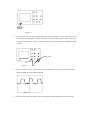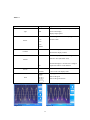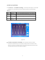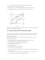
1
INSTRUCTION MANUAL Models 2530 & 2532 Digital Storage Oscilloscopes Model 2530 Model 2532 25 MHz, 250 MSa/s 40 MHz, 500 MSa/s General Safety Summary Review the following safety precautions to avoid injury and prevent damage to this product or any products connected to it. To avoid potential hazards, use this product only as specified. Only qualified personnel should perform service procedures. To Avoid Fire or Personal Injury Use Proper Power Cord. Use only the power cord specified for this product and certified for the country of use. Connect and Disconnect Properly. Do not connect or disconnect probes or test leads while they are connected to a voltage source. Ground the Product. This product is grounded through the grounding conductor of the power cord. To avoid electric shock, the grounding conductor must be connected to earth ground. Before making connections to the input or output terminals of the product, ensure that the product is properly grounded. Connect the Probe Properly. The probe ground lead is at ground potential. Do not connect the ground lead to an elevated voltage. Observe All Terminal Ratings. To avoid fire or shock hazard, observe all ratings and marking on the product. Consult the product manual for further ratings information before making connections to the product. Do Not Operate Without Covers. Do not operate this product with covers or panels removed. Avoid Exposed Circuitry. Do not touch exposed connections and components when power is present. Do Not Operate With Suspected Failures. If you suspect there is damage to this product, have it inspected by qualified service personnel. Do Not Operate in Wet/Damp Conditions. Do Not Operate in an Explosive Atmosphere. Keep Product Surfaces Clean and Dry. Symbols and Terms on the Product. Protective Ground (Earth) Terminal. CAUTION. Refer to user manual. Caution indicates a hazard to property including this product 2 Introduction Description The 2530 & 2532 Digital Storage Oscilloscope is a light-weight benchtop oscilloscope for viewing waveforms and taking measurements. The 2530/2532 is an ideal education and training tool and also well suited for applications in service and repair. Key Features 40 MHz bandwidth, 500MSa/s sample rate with color display (model 2532) 25 MHz bandwidth, 250MSa/s sample rate with monochrome display (model 2530) 4000 point record length for each channel One touch automatic setup for ease of use (Auto) Save/Recall setup and waveform data Capture, save and analyze waveform data and measurement results with the included EasyScope Application Software Cursors with readouts Eleven automatic measurements Waveform averaging and peak detection Math functions: +, -, / and × operations Fast Fourier Transformation (FFT) Extensive Trigger capabilities: Pulse Width trigger, Video trigger capability with line-selectable triggering, External trigger Variable persistence display Built in trigger frequency counter 3 Table of Content Chapter 1 Getting Started................................................................6 1.1 Installation................................................................................................................. 6 1.2 Functional check ....................................................................................................... 6 1.3 Probe handling .......................................................................................................... 8 1.3.1 Probe Safety ........................................................................................................... 8 1.3.2 Probe Compensation .............................................................................................. 8 1.3.3 Probe Attenuation Setting ...................................................................................... 9 1.4 Self Calibration ....................................................................................................... 10 Chapter 2 Main Control Sections Overview .............................. 11 2.1 Vertical System ........................................................................................................11 2.2 Horizontal System................................................................................................... 13 2.3 Trigger System ........................................................................................................ 15 2.3.1 Signal Source ....................................................................................................... 16 2.3.2 Trigger Type......................................................................................................... 16 2.3.3 Coupling............................................................................................................... 19 2.3.4 Position ................................................................................................................ 19 2.3.5 Slope & Level ...................................................................................................... 19 2.4 Acquisition system .................................................................................................. 20 2.5 Display System ....................................................................................................... 23 2.5.1 X-Y Format .......................................................................................................... 25 2.6 Measurement system............................................................................................... 25 2.6.1 Graticule Measurement ........................................................................................ 26 2.6.2 Cursor Measurement ............................................................................................ 26 2.6.3 Auto Measurement ............................................................................................... 27 2.7 Utility System ......................................................................................................... 30 2.7.1 System status........................................................................................................ 31 2.7.3 Self Calibration .................................................................................................... 31 2.7.4 Self Test................................................................................................................ 31 2.8 Save/Recall System................................................................................................. 32 Chapter 3 Operating Basics........................................................36 3.1 Display Area............................................................................................................ 35 3.2 Using the Menu System .......................................................................................... 36 3.3 Using the default setup............................................................................................ 37 3.4 Using the auto setup................................................................................................ 37 3.5 Using the ADJUST knob......................................................................................... 39 3.6 Setting up the Vertical System ................................................................................ 40 3.6.1 Setting up the CH1、CH2 Channels.................................................................... 40 3.6.2 Using the Vertical Position knob and Volts/Div knob .......................................... 44 3.6.3 Using Ref ............................................................................................................. 44 3.7 Math Functions ....................................................................................................... 45 4 3.8 Setting up the Horizontal system ............................................................................ 49 3.8.1 Horizontal control knobs...................................................................................... 49 3.8.2 Window Zone....................................................................................................... 49 3.8.3 Trigger holdoff ..................................................................................................... 50 3.9 Set trigger system.................................................................................................... 50 3.10 Menu and control button ....................................................................................... 51 3.11 Connectors ............................................................................................................ 51 Chapter 4 Application Examples...................................................53 4.1Taking Simple Measurements .................................................................................. 53 4.2 Taking Cursor Measurements ................................................................................. 54 4.2.2 Measuring Ring Amplitude.................................................................................. 55 4.3 Capturing a Single-Shot signal ............................................................................... 55 4.4 Analyzing signal details .......................................................................................... 56 4.4.1 Looking at a Noisy Signal.................................................................................... 56 4.4.2 Separating the Signal from the Noise................................................................... 56 4.5 Triggering on a Video Signal .................................................................................. 56 4.5.1 Triggering on a Video Field ................................................................................. 56 4.5.2 Triggering on Video Lines ................................................................................... 57 4.6 Application for the X-Y function ............................................................................ 57 4.7 Analyzing a Differential Communication Signal .................................................... 58 Chapter 5 Prompt messages and troubleshooting hints.................60 Appendix A: Specifications...........................................................62 Appendix B: Default setup............................................................65 Appendix C: Sample Rate versus Timebase Setting .....................66 Appendix D: Daily Maintenance and Cleaning ............. 66 Appendix E: Index ........................................................................68 Appendix F: Service and Warranty Information ...........................69 5 Chapter 1 Getting Started This Chapter describes the following: ◆ Installation ◆ Basic functional check ◆ Probe check and compensation ◆ Setting of probe attenuation factor ◆ Self calibration procedure 1.1 Installation Inspection Inspect the shipping container and the product for damage. B+K Precision distributor. In case of any damage, notify your authorized Make sure all the accessories as described in the specification chapter are included. Power Source Connect your instrument to an AC power outlet delivering 100 – 240V, 47 – 440 Hz. Use the power cord provided or a comparable cord with an Earth ground connector. Security Loop The instrument provides a security loop located in the rear panel of the instrument. Use a security cable or a security lock to secure your instrument to your location. 1.2 Functional check Perform this check to make sure your instrument is operating correctly. 1. Power On the oscilloscope. Press the “DEFAULT SETUP” button. Note that the probe default attenuation is 10X. 6 ON/ OFF button Figure 1- 2 2. Set the switch to 10X on the included probe and connect it to channel 1 on the oscilloscope. To do this, align the slot in the probe connector with the key on the CH 1 BNC, push to connect, and twist to the right to lock the probe in place. Connect the probe tip and reference lead to the PROBE COMP connector. PROBE COMP CH1 Figure 1-3 3. Press the “AUTO” button. After a few seconds, you should see a square wave signal with a 1KHz frequency and about 3V peak-peak amplitude Figure 1- 4 4 Press the “CH1” button two times to remove the signal from CH1. Repeat steps 2) and 3) for CH2. 7 1.3 Probe handling 1.3.1 Probe Safety A guard around the probe body provides a finger barrier for protection from electric shock. Figure 1-5 Connect the probe to the oscilloscope and connect the ground terminal to ground before you take any measurements. WARNING ● To avoid electric shock when using the probe, keep fingers behind the guard on the probe body. ● To avoid electric shock while using the probe, do not touch metallic portions of the probe head while it is connected to a voltage source. 1.3.2 Probe Compensation Perform this adjustment to match your probe to the input channel. This should be done whenever you attach a probe to any input channel for the first time. 8 Figure 1-6 1. Set the Probe option attenuation in the channel menu to 10X. Set the switch to 10X on the probe and connect the probe to channel 1 on the oscilloscope. If you use the probe hook-tip, ensure a proper connection by firmly inserting the tip onto the probe. 2. Attach the probe tip to the PROBE COMP~3V connector and the reference lead to the PROBE COMP Ground connector. Display the channel and then push the“AUTOSET” button. 3. Check the shape of the displayed waveform. Over compensated Correctly Compensated Under compensated Figure 1-7 4. If necessary, use a non-metallic tool to adjust the trimmer capacitor on the probe for to resemble the Correctly Compensated wave shape as much as possible. Repeat as necessary. 1.3.3 Probe Attenuation Setting Probes are available with various attenuation factors which affect the vertical scale of the signal. If you change the Attenuation switch on the probe, you also need to change the attenuation setting on the oscilloscope accordingly. Note. The default setting for the Probe option is 10X. Be sure that the Attenuation switch on the probe matches the Probe option in the oscilloscope. Switch 9 settings are 1X and 10X. Note. When the Attenuation switch is set to 1X, the probe limits the bandwidth of the oscilloscope to 6MHz. To use the full bandwidth of the oscilloscope, be sure to set the switch to 10X. 1.4 Self Calibration The self calibration routine lets you optimize the oscilloscope’s signal path for maximum measurement accuracy. You can run the routine at any time but should always run the routine if the ambient temperature changes by 5℃ or more. To compensate the signal path, disconnect any probes or cables from the front-panel input connectors. Then, push the UTILITY button, select the “Do Self Cal” option and follow the directions on the screen. 10 Chapter 2 Main Control sections overview The front panel is divided into easy-to-use functional areas. This chapter provides you with a quick overview of the main controls. Figure 1- 1 Front Panel Controls To use your oscilloscope effectively, you need to familiarize yourself with the following control sections: ◆ Vertical System ◆ Horizontal System ◆ Trigger System ◆ Acquisition System ◆ Display System ◆ Measurement System ◆ Utility Menu ◆ Store/Recall Menu 2.1 Vertical System Each channel has a vertical control menu which appears after pressing the CH1 or CH2 button. The vertical controls are used to size and position the signals and to turn the waveform on or off. Below is a figure of the vertical system controls. 11 ` Figure 2-1 Table 2-1 Vertical Control menu Menu Coupling BW limit Volts/Div Probe Invert Settings DC AC GND On/Off Coarse Fine 1X 10X 100X 1000X on off Explanation Both AC and DC components of the input signal are passed on to the oscilloscope The DC component is blocked, only the AC component of the input signal is passed through. Signals below 10Hz are attenuated The waveform is disconnected from the oscilloscope Limits the bandwidth to 20 MHz, in order to reduce display nose and to filter out unwanted high frequency components Selects the resolution of the Volts/Div knob. Coarse defines a 1-2-5 sequence. Fine changes the resolution to small steps between the coarse settings Set to match the type of probe you are using to ensure correct vertical readouts Waveform inverted Invert function is off, original waveform is displayed. Vertical POSITION knob :Use the VERTICAL POSITION knobs to move waveforms up or down on the screen. Volts/Div knob :Use the VOLTS/DIV knobs to control how the oscilloscope amplifies or attenuates the source signal. When you turn the VOLTS/DIV knob, the oscilloscope increases or decreases the vertical size of the waveform on the screen with respect to the ground level. Press the“Volt/div” knob to toggle between “Coarse” and“ Fine” adjustment of the Volt/Div setting. GND Coupling. Use GND coupling to display a zero-volt waveform. Internally, the channel input is connected to a zero-volt reference level. Fine Resolution:The vertical scale readout displays the actual Volts/Div setting while in the fine resolution setting. Changing the setting to coarse does not change the vertical scale until the VOLTS/DIV control is adjusted. 12 Remove the Waveform from the display: Push the CH1 or CH2 button to display the respective vertical menu. Push CH1 or CH2 button again to remove the waveform. Note: ● If DC coupling is active,you can quickly measure the DC component of the signal by simply noting its distance from the ground symbol. ● If the channel is set to AC coupling,the DC component of the signal is blocked allowing you to use greater sensitivity to display the AC component of the signal. 2.2 Horizontal System The horizontal controls change the horizontal scale and position of waveforms. The horizontal center of the screen is the time reference for waveforms. Changing the horizontal scale causes the waveform to expand or contract around the screen center. The horizontal position knob changes the position of the trigger point relative to the center of the screen. Below is a figure of the front panel horizontal systems controls. Figure 2- 2 Table 2- 2 Horizontal Control Menu: Menu Main Win Zone Window Holdoff Holdoff Reset Explanation Display the waveform Define a window (zoom window) by adjusting the cursor position using the Horizontal control knobs Expand the waveform defined in Win Zone to full screen width Using the Adjust knob to adjust the holdoff time Reset the holdoff time to 100ns The center axis of the vertical scale is GND level. The readout on the top right corner, shows the horizontal position. “M” stands for main time base,“W” stands for window time base (Zoom function, horizontal menu)。The arrow on the top center scale shows the vertical position. 13 Figure 2-3 Horizontal POSITION Knob: Used to control the position of the trigger relative to the center of the screen. When the trigger point (downward arrow) moves outside the acquired waveform, (reaches the left or right edge of the screen) the instrument switches automatically to delayed sweep, indicated by the arrow pointing left or right instead of downwards. In delayed sweep mode, you can use the horizontal Time/Div knob to acquire more detail around the center of the screen. Time/Div Knob: Used to change the horizontal time scale to magnify or compress the waveform. If waveform acquisition is stopped (using the RUN/STOP or SINGLE button), the SEC/DIV control expands or compresses the waveform;Pressing the Time/Div knob resets the horizontal position to zero. Window Zone: Define the zoom area of a waveform section. The Window time base setting cannot be set to a value slower than the main time base setting. Window:Press to expand the zoom area to cover the whole screen. Holdoff:You can use Holdoff to produce a stable display of complex waveforms. holdoff time the oscilloscope will not trigger until the holdoff time has expired. During the For a pulse train, you can adjust the holdoff time so the oscilloscope triggers only on the first pulse in the train. Trigger position Trigger level Figure 2-4 Holdoff time 14 Note: • When you change between the Main, Window Zone, and Window views, the oscilloscope erases any waveform which was saved on the screen using persistence. • Use holdoff to help stabilize the display of aperiodic waveforms. 2.3 Trigger System The trigger determines when the oscilloscope starts to acquire data and display a waveform. The oscilloscope acquires data while waiting for the trigger condition to occur. After it detects a trigger, the oscilloscope continues to acquire enough data so that it can draw the waveform on the display. Below are the trigger section controls: Figure 2-5 “TRIG MENU” Button:press the “TRIG MENU” Button to display the TRIG MENU Figure 2-6 15 LEVEL Knob:Set the trigger level SET TO 50% Button:Use the SET TO 50% button to stabilize a waveform quickly. The oscilloscope automatically sets the Trigger Level about halfway between the minimum and maximum voltage levels. This is useful when you connect a signal to the EXT TRIG BNC and set the trigger source to Ext or Ext/5. FORCE Button:Use the FORCE TRIG button to complete the current waveform acquisition regardless of whether or not the oscilloscope detects a trigger. This is useful for SINGLE acquisitions and Normal trigger mode. 2.3.1 Signal Source You can use the Trigger Source options to select the signal that the oscilloscope uses as a trigger. The source can be any signal connected to the CH1 or CH2 connectors, the EXT TRIG connector or the AC power line (available only with Edge trigger). 2.3.2 Trigger Type The 2530 series supports three types of Trigger signals:Edge,Video and Pulse Trigger. Edge trigger can be used with analog and digital circuits. An edge trigger occurs when the trigger input passes through a specified voltage level with the specified slope. Pulse trigger is used to find pulses with certain pulse widths. Video is used to trigger on fields or lines for standard video waveforms. 16 Table 2-3 Edge Trigger Menu : Menu Setting Type Edge With Edge selected, the rising or falling edge of the input signal is used for the trigger CH1 Triggers on CH1 or CH2 regardless of whether or not the waveform CH2 is displayed。 EXT Source EXT/5 AC Line Slope Explanation Rising Uses the signal connected to the EXT TRIG front-panel BNC as trigger source. Trigger level range is -2.4V to +2.4V Same as EXT but attenuates the applied trigger signal by a factor of five. The trigger level range is extended to +12V to -12V. Uses power line as the trigger source. Trigger coupling is set to DC and the trigger level is 0 volts. Trigger to the rising or falling edge Falling Use the Auto Mode to let acquisition free-run in the absence of a Auto valid trigger condition.. This mode also supports an untriggered, scanning waveform at 100 ms/div or slower time base settings Mode Use this mode when you want to see only valid triggered Normal waveforms. When you use this mode, the oscilloscope does not display a waveform until after the first trigger Single Coupling When you want the oscilloscope to acquire a single waveform, press the “SINGLE ”button DC Passes all components of the signal AC Blocks DC components and attenuates signals below 10 Hz HF Reject Attenuates the high-frequency components above 80 kHz LF Reject Blocks the DC component and attenuates the low-frequency components below 300 kHz 17 Table 2-4 Video Trigger Menu: Menu Type Setting Video Explanation When you select Video Trigger mode, set coupling to AC. Now you can trigger from a NTSC or PAL/SECAM video signal. Source CH1 Select the input source to be the trigger signal. CH2 EXT Ext and Ext/5 use the signal applied to the EXT TRIG connector as the EXT/5 source. Polarity Sync (Normal) Triggers on the negative edge of the sync pulse (Inverted) Triggers on the positive edge of the sync pulse Line Num Select on which part of the video signal you want to trigger All lines Odd field Even Field Standard NTSC Select the video standard for sync and line number count Pal/Secam Table 2-5 Pulse Trigger Menu: A pulse trigger occurs when a pulse is found in a waveform that matches the pulse definition. The When and Set Width menu buttons control the pulse definition. Menu Type Setting Pulse Explanation Select the pulse to trigger the pulse match the trigger condition CH1 Source CH2 EXT EXT/5 When (Positive pulse width less than pulse width setting) Select how to compare the trigger (Positive pulse width larger than pulse width setting) pulse relative to the value (Positive pulse width equal to pulse width setting) (Negative pulse width less than pulse width setting) (Negative pulse width larger than pulse width setting) 18 selected in the Pulse Width option (Negative pulse width equal to pulse width setting) set width Mode Adjust the pulse width with the 20.0ns~10.0s ADJUST knob Auto Select the type of triggering; Normal Normal mode is best for most single Pulse Width trigger applications DC Coupling AC HF Reject LF Reject Hint:Use Pulse Width triggering to trigger on aberrant pulses. 2.3.3 Coupling Use “Coupling” to select which component of the signal to pass on to the trigger circuit. This parameter only applies to Edge or Pulse trigger mode, for Video trigger mode coupling is always set to AC. 2.3.4 Position The horizontal position control establishes the time between the trigger position and the screen center. You can adjust the HORIZONTAL POSITION control to view waveform data before the occurrence of the trigger, after the trigger, or any point in between. When you change the horizontal position of a waveform, you are changing the time between the trigger and the actual center of the display. (This appears to move the waveform to the right or left on the display.). Use a pretrigger setting to acquire waveforms leading up to a trigger event. Use a post trigger setting when you want to acquire waveforms that follow an event. When the trigger point (downward arrow) moves outside the acquired waveform, (reaches the left or right edge of the screen) the instrument switches automatically to delayed sweep, indicated by the arrow pointing left or right instead of downwards. In delayed sweep mode, you can use the horizontal time/Div knob to acquire more detail around the center of the screen. 2.3.5 Slope & Level The Slope and Level controls help to define the trigger. The Slope option (Edge trigger type only) determines whether the oscilloscope finds the trigger point on the rising or the falling edge of a signal. The TRIGGER LEVEL knob controls where on the edge the trigger point occurs. 19 Trig ge r le ve l ca n be ad ju ste d vert ica lly Rising edge Falling edge Figure 2-7 Note: • Press the SINGLE button when you want the oscilloscope to acquire a single waveform • Trigger coupling affects only the signal passed to the trigger system. It does not affect the bandwidth or coupling of the signal displayed on the screen. • Normal Polarity Sync triggers always occur on negative-going horizontal sync pulses. If the video waveform has positive-going horizontal sync pulses, use the Inverted Polarity selection. 2.4 Acquisition system When you acquire a signal, the oscilloscope digitizes the signal and displays the resulting waveform on the screen. The acquisition mode defines how the signal is digitized, and the time base setting affects the time span and level of detail in the acquisition. The sampling rate adjusts automatically to a value suitable for each selected Time/Div scaling factor. Refer to Appendix C for more detailed information. Push the ACQUIRE button to access the Acquisition menu Acquire button Figure 2-8 20 Table 2- 6 Acquire Menu: Menu Set up Explanation Sampling Use to acquire and accurately display most waveforms Peak Detect Use to detect glitches and decrease the possibility of aliasing. Average Select this mode to reduce the displayed random noise. Averages 4 Specify number of averages 16 32 64 128 256 Mode Equ time Select realtime or equivalent sampling Real time The 3 acquisition modes Sample, Peak Detect and Average: Sampling: In this acquisition mode, the oscilloscope samples the signal in evenly spaced intervals to reconstruct the waveform. This mode accurately represents the signal most of the time. Advantage: You can use this mode to reduce random noise. Disadvantage: This mode does not capture rapid variations in the signal that may occur between samples. This can result in aliasing and may cause narrow pulses to be missed. In these cases, you should use the Peak Detect mode to acquire data. Figure 2-9 Sampling mode Peak Detect: Peak Detect finds the maximum and minimum values of a signal. Advantage: In this way, the oscilloscope can acquire and display narrow pulses, which may have otherwise been missed in Sample mode. Disadvantage: Noise will appear to be higher in this mode. 21 Figure 2-10 Peak Detect mode Average: The oscilloscope acquires several waveforms, averages them, and displays the resulting waveform. Advantage: You can use this mode to reduce random noise. Figure 2-11 Average mode Equivalent Time Sampling: The equivalent time sampling mode can achieve up to 20 ps of horizontal resolution (equivalent to 50 GSa/s). This mode is good for observing repetitive waveforms. Real Time Sampling: The maximum sampling rate for the 2530 is 250 MSa/s and 500MSa/s for the 2532. RUN/STOP Button: Press the RUN/STOP button when you want the oscilloscope to acquire waveforms continuously (Run/Stop button is green). Press the button again to stop the acquisition.( Run/Stop button is red) 22 SINGLE Button:Push the SINGLE button when you want the oscilloscope to acquire a single waveform and then stop. (Make sure the Run Stop button is green and the display annunciator is in the Ready state). After the oscilloscope detects a trigger, it completes the acquisition then stops. Each time you push the SINGLE button, the oscilloscope begins to acquire another waveform. Base time: The oscilloscope digitizes waveforms by acquiring the value of an input signal at discrete points. The time base allows you to control how often the values are digitized. Appendix C details the corresponding sampling rate for each time base setting. To adjust the time base to a horizontal scale that suits your purpose, use the Time/DIV knob. Time Domain Aliasing:Aliasing occurs when the oscilloscope does not sample the signal fast enough to construct an accurate waveform record. When this happens, the oscilloscope displays a waveform with a frequency lower than the actual input waveform, or triggers and displays an unstable waveform. Actual high-frequency waveform Apparent low-frequency waveform due to aliasing Sampled points Figure 2-12 2.5 Display System Push the display button to choose how waveforms are presented and to change the appearance of the entire display. Display System Figure 2-13 23 Table 2-7 Options Type Set up Explanation Vectors Vectors fills the space between adjacent sample Dots points in the display Display sample points Persist Off Sets the length of time each sampling point 1 sec remains visible. 2 sec 5 sec Infinite Contrast + Increase the display contrast - Decrease the display contrast YT YT format displays the vertical voltage in relation to time (horizontal scale) Format XY format displays a dot each time a sample is Screen XY acquired on channel 1 and channel 2 Normal set to normal mode Inverted set to invert color display mode Display grids and axes on the screen Turn off the grids Grid Turn off the grids and axes Figure 2-14 Figure 2-15 24 2.5.1 X-Y Format Use the XY format to analyze phase differences, such as those represented by Lissajous patterns. The format plots the voltage on channel 1 against the voltage on channel 2, where channel 1 is the horizontal axis and channel 2 is the vertical axis. The oscilloscope uses the untriggered sample acquisition mode and displays data as dots. In this mode, the sampling default sampling rate is 1 MSa/s and is adjustable from 5kSA/s – 200 MSa/s.. Note:The oscilloscope can capture a waveform in normal YT mode at any sampling rate. You can view the same waveform in XY mode. To do so, stop the acquisition and change the display format to XY. In this mode, the controls operate as followed: • The Channel 1“Volts/div”and vertical “POSITION” controls set the horizontal scale and position. • The Channel 2“Volts/div”and vertical “POSITION” controls continue to set vertical scale and position. The following functions do not work in XY mode: • Reference or math waveform • Cursors • Autoset(resets display format to YT) • Trigger Controls • Horizontal Position Knob • Vector Display Type • Scan Display Note: When the display Type is set to Vectors, the oscilloscope connects the sample points by using digital interpolation. Interpolation mode contain linearity interpolation and sin(x)/x interpolation. Sin(x)/x interpolation is suitable for real time mode and is most effective at 250ns/div or faster time. The oscilloscope automatically switches to the most suitable display type based on the timebase setting. 2.6 Measurement system There are several ways to take measurements. You can use the graticule, the cursors, or make an automated measurement. 25 2.6.1 Graticule Measurement This method allows you to make a quick, visual estimate. For example, you might look at a waveform amplitude and determine that it is a little more than 100 mV. You can take simple measurements by counting the major and minor graticule divisions involved and multiplying by the scale factor. For example, if you counted five major vertical graticule divisions between the minimum and maximum values of a waveform and knew you had a scale factor of 100 mV/division, then you could easily calculate your peak-to-peak voltage as follows: 5 divisions x 100 mV/division = 500 mV. 2.6.2 Cursor Measurement This method allows you to take measurements by moving the cursors, which always appear in pairs, and reading their numeric values from the display readouts. Access the Cursor menu by pressing the Cursor button. Cursors Button Figure 2-16 Table 2-7 Functional Menu of the Cursor Menu Setting Comment Type Voltage Select and display the measurement cursors. Time amplitude and the vertical cursor measures time and frequency. The horizontal cursor measures Off Source CH1 Select the wave form source to be measured by the cursors CH2 MATH REFA REFB Cur1 Cur2 Activate Cursor 1. Activate Cursor 2. Use the ADJUST knob to adjust the cursor position Use the ADJUST knob to adjust the cursor position. 26 Figure 2-17 Voltage Cursor: Voltage cursors appear as horizontal lines on the display and measure the vertical parameters. Time Cursor: Time cursors appear as vertical lines on the display and measure the horizontal parameters. Moving Cursors:Use the ADJUST knob to move cursor1 and cursor2. Cursors can be moved when the cursor menu is displayed. 2.6.3 Auto Measurement “MEASURE”: When you take automatic measurements, the oscilloscope does all the calculating for you. Because this method relies on the digital samples of the waveform, this method is more accurate than graticule or cursor measurements. Auto Measurement button Figure 2-18 Press the ‘MEASURE’ button. There are 11 types of measurements available. You can display up to five measurements at a time. To define each of the 5 measurements, do the following: 27 1. Press one of the five option buttons corresponding to measurement 1 – 5 . This will open a sub menu. 2. Enter the Source of the measurement and the measurement type 3. Press the bottom option button to turn the measurement on If you want to display all eleven measurements at once, select “All Mea” from the sub menu (step 2) Voltage Measurements:Max, Min, Peak-Peak, Average, Vrms。 Figure 2-19 Time Measurements:Rise time, Fall time, Frequency, Period, positive pulse width, negative pulse width. Figure 2-20 28 2-8 Measurement Types: Measure Type Vpp Introduction Vmax examines the entire 2500 point waveform record and displays the maximum value Vmin examines the entire 2500 point waveform record and displays the minimum value Vpp calculates the absolute difference between the maximum and minimum peaks of the entire waveform Vavg Count the arithmetic average value in the record Vmax Vmin Vrms Rise Fall + Width - Width Prd Freq Calculates a RMS measurement of the first complete cycle of the waveform Rise Time measures the time between 10% and 90% of the first rising edge of the waveform. Fall Time measures the time between 90% and 10% of the first falling edge of the waveform. + Width measures the time between the first rising edge and the next falling edge at the waveform 50% level. -Width Measures the time between the first falling edge and the next rising edge at the waveform 50% level. Measure the Period Measure the Frequency * The instrument displays 2500 points. The full record length of 4000 points can be retrieved from internal memory with the included EasyScope application Software Select “All measurements”to display all eleven measurements at once. Fig. 2.21 29 2.7 Utility System ”: The Utility System Button。 Utility Setup button Figure 2-22 Table 2- 9 Utility Menu options Option System Status Sound Counter Language DO self cal Do Self Test Setting On Off English Screen Test Keyboard Test LED Test Comment Displays information about the hardware and software configuration This option turns the button beep on or off Turn the Trigger frequency counter On/Off* Run the Self Calibration routine Run a screen test Run a keyboard test Run the LED test Press the UTILITY button to see the “Utility menu” Figure 2-23 Figure 2-24 30 2.7.1 System status Selecting “System Status” from the Utility Menu to display information about a particular unit Table 2-10 Display Explanation Startup Times Counts the times the unit was turned on/off. Software version Gives the software version Hardware Version Gives the hardware version Product type Lists the model number Serial No. List the unit’s serial number 2.7.3 Self Calibration Before executing the Self Calibration routine, disconnect all probes and leads from the input connector. Then press the “Utility” button and select “Do self cal” to show the self Calibration Menu. Figure 2-25 2.7.4 Self Test Table2-12 Press“UTILITY”→“Do Self Test” Option Introduction Screen Test Run Screen Test Program Keyboard Test Run Keyboard Test Program LED Test Run LED Test Program 31 (1) Screen Test: Select “Screen Test” to enter the screen mode. Press the SINGLE key to continue,press RUN/STOP to exit. (2) Keyboard Test Select “Keyboard Test” to enter the key test mode. The shapes with two arrows beside them represent the front panel knobs. The squares represent the knob presses for scale knobs. Test all keys and knobs and verify that all the backlit buttons illuminate correctly. Press RUN/STOP 3 times to exit. (3) LED test Select “LED Test” to run the LED test procedure. Continually press the SINGLE key to step through all the buttons. Press RUN/STOP to exit. 2.8 Save/Recall System Use this menu to save and recall waveforms and setups. The instrument can store/recall 10 setups and 10 waveforms. Save/Recall control button Figure 2-26 SAVE/RECALL SETUP SAVE/RECALL Setup: The complete setup is stored in nonvolatile memory. When you recall the setup, the oscilloscope will be in the mode from which the setup was saved. The oscilloscope will automatically save the current setup if you wait three seconds after the last change before you power off the oscilloscope. The oscilloscope recalls this setup the next time you apply power. Up to 10 setups can be recalled/stored. 32 Table 2-13 Menu Type Setting Setups Setup NO.1 to NO.10 Save Recall Explanation Menu for the Storage/Recall setting in the oscilloscope Select the memory location to/from which you want to save/recall a setup Save a setup to the memory location selected Recall a setup from the memory location selected Figure 2-27 RECALL FACTORY: You can use this option to recall the factory setup. Select type Factory then press LOAD. Figure 2-28 33 SAVE/RECALL WAVEFORM SAVE/RECALL CAPTURED WAVEFORM: The oscilloscope must display any waveform that you want to save. The oscilloscopes can store ten captured waveforms in nonvolatile memory. Table 2-15 Option Setup Introduction Type waveforms Menu for the Storage/Recall waveforms in the oscilloscope waveform NO.1 to NO.10 Save/Recall the waveforms in the currently position Save Accomplish the storage Recall Recall the storage in the “waveform” operation Figure 2-29 ■ SAVE/RECALL REFERENCE WAVEFORM:The oscilloscopes can store two reference waveforms in nonvolatile memory. The oscilloscope can display 2 reference waveforms at a time. Reference waveforms are not adjustable, but the oscilloscope does display the horizontal and vertical scales at the bottom of the screen. (more details see Chapter 3) 34 Chapter 3 Operating Basics The previous chapter introduced the main functional blocks of the instrument. This chapter explains in more detail how to set up the oscilloscope to view signals and to make measurements. Explanation of Display area Using the Menu System Using the Default Setup Using the Auto Setup Using the Universal knob Setting up the Vertical System Setting up the Horizontal System Setting up the Trigger System Using Math and FFT Functions Menu and Control Buttons Connectors 3.1 Display Area Figure 3-1A 1 Figure 3-2B Acquisition mode Sampling mode Peak detect mode 35 Average mode 2 Trigger status □ Armed. The oscilloscope is acquiring pretrigger data. All triggers are ignored in this state. Ready. All pretrigger data has been acquired and the oscilloscope is ready to accept a trigger T Trig’d. The oscilloscope has received a trigger signal and is acquiring the post trigger data. Stop. The oscilloscope has stopped acquiring waveform data. Single Trigger mode: The oscilloscope has completed a Single acquisition. Auto. The oscilloscope is in auto mode and is acquiring waveforms in the absence of a trigger signal. □ Scan. The oscilloscope is acquiring and displaying waveform data continuously in scan mode. 3 Marker shows horizontal trigger position. Turn the HORIZONTAL POSITION knob to adjust the position of the marker. 4 Read out of the time at the center graticule. 5 The marker indicates the edge and pulse width trigger level. 6 The on-screen markers show the ground reference points of the displayed waveforms. If there is no marker, the channel is not displayed. 7 Readout shows the vertical factor of the channels 8 Readout of the main time base setting 9 Readout of the window time base setting, when window mode (zoom) is activated 10 Trigger source for trigger section 11 Icon indicates selected trigger types 12 Readout of edge and pulse width trigger level. Indicates the line number when in Video trigger mode 13 Displays Reference A Voltage and time base setting if REFA is activated 14 Displays Reference B Voltage and time base setting if REFB is activated 15 Displays reading of Trigger reference counter if activated 3.2 Using the Menu System When you press a front-panel button, the oscilloscope displays the corresponding menu on the right side of the screen. The menu shows the options that are available when you press the unlabeled option buttons directly to the right of the screen. 36 The oscilloscope uses three methods to display menu options: ■ Circular List: The oscilloscope sets the parameter to a different value each time you press the option button. ■ Action: The oscilloscope displays the type of action that will immediately occur when you push an Action option button. For example, when you push the DISPLAY Menu button and then push the Contrast Increase option button, the oscilloscope changes the contrast immediately. ■ Radio: The oscilloscope uses a different button for each option. The currently-selected option is highlighted. Circular list Action Radio Figure 3-3 3.3 Using the default setup The oscilloscope is set up for normal operation when it is shipped from the factory. This is the default setup. To recall this setup, press the DEFAULT SETUP button. The options, buttons and controls that change settings when you press the DEFAULT SETUP button, refer to appendix B. The DEFAULT SETUP button does not reset the following settings: ● Saved reference waveform files ● Saved setup files ● Display contrast ● Calibration data 3.4 Using the auto setup The 2530 & 2532 Digital Storage Oscilloscope has an auto setup function which can identify the type of waveform and automatically adjust controls to produce a usable display of the input signal. Press the Auto button to activate this mode 37 Table 3-1 Auto set the function Menu : Option Set Up Comment Auto set the screen and display multiple cycles Auto set the screen and display a single cycle Auto set and show the rise time Auto set and show the fall time ( Causes the oscilloscope to recall the previous setup (Undo Setup) Figure 3-3 When you press the AUTOSET button, the oscilloscope identifies the type of waveform and adjusts controls to produce a usable display of the input signal. Autoset determines the trigger source based on the following conditions: ● If a signal is applied to both channels, the instrument displays the channel with the lowest frequency ● If no signals are found, the oscilloscope displays Channel 1. Table 3-2 Oscilloscope settings for Auto mode Function Setting Acquire Mode Set to Sampling Acquire Type Equ time (Equivalent Sampling) Display Format Y-T Display Type Set to Dots for a video signal, set to Vectors for an FFT spectrum; otherwise, unchanged Vertical Coupling Set to DC or AC according to the input signal 38 Volts/DIV Adjusted VOLTS/DIV Coarse adjustability Signal inverted off Horizontal position Adjusted Time/div Adjusted Trigger type Edge Trigger source Auto detect the channel which has the input signal Trigger slope Rising Trigger mode Auto Trigger coupling DC Trigger holdoff Minimum Trigger level Set to 50% 3.5 Using the ADJUST knob ADJUST knob Figure 3-4 The 2530 Series Digital Storage Oscilloscope comes with an ADJUST knob. Use this knob to set up the holdoff time, cursor positions for measurements, pulse width and the Video Line number Adjust holdoff time 1. Press the HORI MENU button to show the “Hori Menu”. 2. Press the holdoff option button 3. Turn the ADJUST knob to adjust the holdoff time。 Cursor Measure 1. Press the CURSORS button to display the cursor Menu. 2. Press the “Source” option button to select the source. 39 3. Press the Cur1 option button, turn the ADJUST knob to adjust Cur1. 4. Press the Cur2option button, turn the ADJUST knob to adjust Cur2. 5. The value of Cursor1 and Cursor2 is incremented and displayed on the top right of the screen. Pulse Setup 1. Press the “TRIG MENU” button to display the Trigger Menu. 2. Press the “Type” Option and choose “Pulse”. 3. Press the “ Set Width” button. 4. Turn the ADJUST knob to adjust the pulse width. Set the Video Line Number 1. Press “TRIG MENU” to show the Trigger Menu 2. Press the “Type” button and select Video trigger. 3. Press the “Sync” operation button, select the line number. 4. Turn the ADJUST knob to adjust Line Num. 3.6 Setting up the Vertical System 3.6.1 Setting up the CH1, CH2 Channels Each channel has its own separate Menu. The items are set up separately according to each channel. 1. Set up the coupling mode Apply a sine wave signal with a DC offset to CH1 • Press“CH1”→“Coupling”→“AC”. Set AC coupling mode. Now the DC component of the signal is blocked. Figure 3-5 • Press“CH1”→“Coupling”→“DC”. Set DC coupling mode. Both the DC and AC component of the signal will be passed on and displayed on the screen. 40 Figure 3-6 • Press“CH1”→“Coupling”→“GND”. Select GROUND mode to disconnect the input signal. Figure 3-7 2.Volts/Div settings Vertical scaling can be adjusted in 2 modes, Coarse and Fine. The vertical sensitivity range is 2mV/div~ 5V/div scale。 Take CH1 for example • Press“CH1”→“Volts/Div”→“Coarse”. This is the default setting of Volts/Div,and it allows adjustment of the vertical scale in a 1-2-5-step sequence starting from 2mV/Div,5mV/Div,10mv/div up to 5V/Div. 41 Figure 3-10 ●Press“CH1”→“Volts/Div”→“Fine”. This setting changes the vertical scale to small steps between the coarse settings. It is useful when you need to adjust the vertical scale in small steps to set a specific value. Figure 3-11 4. Probe Attenuation The setting of the attenuation coefficient in the menu must match the setting of the probe., If the attenuation coefficient is 10 :1, the input coefficient should be set to 10X in order to obtain correct readings. Example: Probe connected to CH1 has factor of 100:1 ● Press“CH1”→“Probe”-“100X. 42 Figure 3-12 5. To invert a waveform ● Press“CH1”→“Invert”→“off” Figure 3-13 ●Press“CH1”→“Invert”→“on” Figure 3-14 43 3.6.2 Using the Vertical Position knob and Volts/Div knob 1. The vertical“POSITION”knob is used to adjust the vertical position of each channel (including MATH and REF wave). This knob’s resolution varies according to the currently set scale factor (set by Volts/Div knob). 2. The Volts/Div knob adjusts the vertical resolution of each channel, (including the MATH and REF waves). In Coarse mode, the scale factor steps are adjustable in a 1-2-5 step sequence. To magnify the display signal turn the knob clockwise, to decrease the waveform turn counter clockwise. Pressing the Volts/Div knob toggles between Coarse and Fine mode. In the Fine mode, the knob adjusts the Volts/Div factor in small increments between the coarse settings. 3. When you adjust the vertical position of a channel waveform, the vertical position information will be displayed on the bottom left of the screen. 3.6.3 Using Ref The reference control saves waveforms to nonvolatile waveform memory. The reference function becomes available after a waveform has been saved. Press the Ref button to display the reference waveform menu Table 3-7 Option Setup Comment Source CH1 Choose the waveform display you want to store. CH2 if the corresponding channel is turned off A Choose the store/recall location REF This option is turned OFF B Save Store the current waveform to the selected location REFA/REFB On Determines which reference wave from is visible on the screen Off How to Save and Recall waveforms: 1. Press the “REF” menu button to display the reference waveform menu. 2. Select channel1 or channel2 3. Turn the vertical “POSITION” knob and “Volt/div” knob to adjust the vertical position and scale appropriately. 4. Press Save to save waveforms on the current screen as ref waveforms. 5. Recall reference waveform by setting REF A or REB to On Note: The Ref function is not available in XY mode You cannot adjust the horizontal position and scale of the reference waveform. 44 3.7 Math Functions This oscilloscope supports arithmetic math functions +,-,*, and FFT operations which depending on the operation, can be applied to either channel or both channels. Press the MATH MENU button to display the waveform math operations. Table 3-3 MATH Menu Function Set up Comment Operation +, -, *, /, FFT Source 1 plus Source 2 CH1 Invert on Invert the CH1 waveform off CH2 Invert on Invert the CH2 waveform off Table 3-4 Operation + - * / FFT Set up Introduction CH1+CH2 Add CH1 and CH2 waveforms CH1-CH2 Subtract channel 2 from channel 1 waveform CH2-CH1 Subtract channel 1 from channel 2 waveform CH1*CH2 Multiply CH1 with CH2 waveform CH1/CH2 CH1 divided by CH2 waveform CH2/CH1 CH2 divided by CH1 waveform Fast Fourier Transform Figure 3-15 45 1. FFT Spectrum Analyzer The FFT process mathematically converts a time-domain signal into its frequency components. You can use the Math FFT to analyze the following type of signals: • Characterize noise in DC Power supplies • Test the impulse response of filters and systems • Analyze vibration • Analyze harmonics in power lines • Measure harmonic content and distortion in a system Table 3-5 FFT Option Source Set Introduction CH1 Select the channel to which you want to apply the FFT CH2 Hanning Window operation Select the FFT window type Hamming Rectangular Blackman 1X FFT ZOOM Changes the horizontal magnification of the FFT display 2X 5X 10X Scale Vrms Set Vrms to be the Vertical Scale unit dBVrms Set dBVrms to be the vertical Scale unit Figure 3-16 46 Explanation of Figure 3-16: In this example the position at the center graticule is 3kHz (Pos: 3.00 kHz), the frequency of the second harmonic. The vertical scale is set to 100mVrms/Div and the horizontal scale is set to 12.5kHz (1.25kHz x 10 zoom factor). The window type is Blackman To use the Math FFT mode, you need to perform the following tasks: 1. Set up the source YT (time-domain) waveform. ● Press AUTOSET to display a YT waveform. ● Turn the VERTICAL POSITION knob to move the YT waveform to the center vertically (zero divisions). ● Turn the HORIZONTAL POSITION knob to position the part of the YT waveform that you want to analyze in the center eight divisions of the screen. The oscilloscope calculates the FFT spectrum using the center 1024 points of the time-domain waveform. ● Turn the VOLTS/DIV knob to ensure that the entire waveform remains on the screen. ● Turn the Time/DIV knob to provide the resolution you want in the FFT spectrum. ● If possible, set the oscilloscope to display many signal cycles. To set up the FFT display, follow these steps: - Push the MATH MENU button. - Set the Operation option to FFT. - Select the Math FFT Source channel. 2. Displaying the FFT Spectrum Press the MATH MENU button to display the Math Menu. Use the options to select the Source channel, Window algorithm, and FFT Zoom factor. You can display only one FFT spectrum at a time 3. Select an FFT window Windows reduce spectral leakage in the FFT spectrum. The FFT assumes that the YT waveform repeats forever. With an integral number of cycles, the YT waveform starts and ends at the same amplitude and there are no discontinuities in the signal shape A non-integral number of cycles in the YT waveform causes the signal start and end points to be at different amplitudes. The transitions between the start and end points cause discontinuities in the signal that introduce high-frequency transients. There are 4 FFT windows. Each window has trade-offs between frequency resolution and amplitude accuracy. Your source waveform characteristics along with your measurement priorities help determine which window to use. Use the following guidelines to select the best window. 47 Table 3-6 Window Rectangular Characteristics Application/ Measurement Best frequency resolution, worst Symmetric transients or bursts. magnitude resolution. This is Equal-amplitude sine waves with essentially the same as no window. fixed frequencies. Broadband random noise with a relatively slowly varying spectrum. Better frequency, poorer magnitude Sine, periodic, and narrow-band Hanning/ accuracy than Rectangular. random noise. Asymmetric Hamming Hamming has slightly better transients or bursts. frequency resolution than Hanning. Blackman Best magnitude, worst frequency Single frequency waveforms, to resolution. find higher order harmonics. 4. Magnifying and Positioning an FFT Spectrum You can magnify and use cursors to take measurements on the FFT spectrum. The oscilloscope includes an FFT Zoom option to magnify horizontally. To magnify vertically, you can use the vertical controls. 5. Measuring an FFT Spectrum Using Cursors You can take two types of measurements on FFT spectrums: magnitude (in dB) and frequency (in Hz). Magnitude is referenced to 0 dB, where 0 dB equals 1 Vrms. You can use the cursors to take measurements at any zoom factor. Use horizontal cursors to measure magnitude and vertical cursors to measure frequency. Make sure to select the “MATH” as source in the cursor menu.. The options display the delta between the two cursors, the value at cursor 1 position, and the value at cursor position. Delta is the absolute value of cursor 1 minus cursor 2. NOTE: ● The FFT of a waveform that has a DC component or offset can cause incorrect FFT waveform magnitude values. To minimize the DC component, choose AC Coupling on the source waveform. ● To display FFT waveforms with a large dynamic range, use the dBVrms scale. The dBVrms scale displays component magnitudes using a log scale. ● The Nyquist frequency is the highest frequency that any real-time digitizing oscilloscope can acquire without aliasing. This frequency is half that of the sample rate, provided it is within the analog bandwidth of the oscilloscope. Frequencies above the Nyquist frequency will be under sampled, which causes aliasing. 48 3.8 Set up the Horizontal system 3.8.1 Horizontal control knobs The oscilloscope shows the time per division in the center of the bottom status bar. The horizontal controls change the horizontal scale and position of waveforms. The horizontal center of the screen is the time reference for waveforms. Changing the horizontal scale causes the waveform to expand or contract around the screen center. The horizontal position knob changes the position of the trigger point relative to the center of the screen. The oscilloscope digitizes waveforms by acquiring the value of an input waveform at discrete points. The time base also controls the sampling rate of this digitizing process. The sampling rate adjusts automatically to a value suitable for each selected Time/Div scaling factor. Refer to Appendix C for more detailed information. ■ Horizontal POSITION knob:Adjusts the horizontal position of both channels and math waveforms. The resolution of this control varies according to the horizontal scale factor. ■ Time/Div knob:Selects the horizontal scale factor for the main or the window time base. When Window Zone is enabled, it changes the width of the window zone by changing the window time base. ■ Display scan mode: When the Time/DIV control is set to 100 ms/div or slower and the trigger mode is set to Auto, the oscilloscope enters the scan acquisition mode. In this mode, the waveform display updates from left to right. In this mode, trigger or horizontal position control of waveforms is disabled. Figure 3-18 scan mode display 3.8.2 Window Zone Use the Window Zone option to define a segment of a waveform you want to see in greater detail. The Window time base setting cannot be set slower than the Main time base setting. Adjust the Horizontal 49 Position and Time//Div controls to enlarge or minimize waveforms in the Window Zone Figure 3-19 Window setup Figure 3-20 Window zone 3.8.3 Trigger holdoff If you want to change the holdoff time, do the following: 1. Press the HORI MENU button to show the Horizontal Menu 2. Press Holdoff。 3. Adjust the ADJUST knob to change the holdoff time until the waveforms triggers reliably. 3.9 Set trigger system The trigger determines when the oscilloscope starts to acquire data and display a waveform. When a trigger is set up properly, the oscilloscope converts unstable displays or blank screens into meaningful waveforms. The trigger Control area includes the Level knob, TRIG MENU button, SET TO 50% button and FORCE 50 button. . ■ “LEVEL”knob:The LEVEL knob sets the amplitude level the signal must cross to cause an acquisition. ■ “SET TO 50%”: The trigger level is set to the vertical midpoint between the peak values of the trigger signal. ■ “FORCE”button: Completes an acquisition regardless of an adequate trigger signal. This button is usually used in normal mode and single mode 3.10 Menu and control button Figure 3-23 ■ CURSORS:Display the Cursor Menu ■ MEASURE:Display the automated measurements menu. ■ ACQUIRE:Display the Acquire Menu. ■ DISPLAY:Display the Display Menu. ■ UTILITY:Display the Utility Menu. ■ SAVE/RECALL: Display the Save/Recall Menu for setups and waveforms. ■ DEFAULT SETUP:Recall the factory setup. ■ AUTO:Automatically sets the oscilloscope controls to produce a usable display of the input signals. ■ RUN/STOP:Continuously acquires waveforms or stops the acquisition. Note:If waveform acquisition is stopped (using the RUN/STOP or SINGLE button), the TIME/DIV control expands or compresses the waveform. ■ SINGLE:Acquire a single waveform and then stop. 3.11 Connectors 51 Figure 3-24 ■ Probe component: Voltage probe compensation output and ground. Use to electrically match the probe to the oscilloscope input circuit. ■ CH1、CH2 :Input connectors for waveform display. ■ EXT TRIG: Input connector for an external trigger source. Use the Trigger Menu to select the Ext or Ext/5 trigger source. Note: If you connect a voltage source to a ground terminal, you may damage the oscilloscope or the circuit under test. To avoid this, do not connect a voltage source to any ground terminals. 52 Chapter 4 Application Examples This section presents a series of application examples. These basic examples highlight the features of the oscilloscope and provide you with ideas how you can solve your testing problems using the 2530/2532 oscilloscope. ◆ Taking simple measurements ◆ Taking cursor measurements ◆ Capturing a single-shot signal ◆ Analyzing signal details ◆ Triggering on a video signal ◆ Application of X-Y function ◆ Analyzing a differential communication signal using math functions 4.1 Taking Simple Measurements Example: Observe a unknown signal, display the signal quickly and measure the frequency and peak-to-peak amplitude. 1. Using Auto set To quickly display a signal, follow these steps: 1 Press the CH 1 button , set the Probe option attenuation to 10X and set the switch to 10X on the probe. 2. 3. Connect the channel 1 probe to the signal. Press the AUTO button. The oscilloscope sets vertical, horizontal, and trigger controls automatically. If you want to optimize the display of the waveform, you can manually adjust these controls. NOTE. The oscilloscope displays relevant automatic measurements in the waveform area of the screen based on the signal type detected. 2. Taking Automatic Measurements The oscilloscope can take automatic measurements of most displayed signals. To measure signal frequency and peak-to-peak amplitude, follow these steps: (1) Measure signal frequency ● Input the signal to channel 1. ● Press the “AUTO” button. ● Press the “MEASURE ”button to see the Measure Menu. 53 ● Press the top option button, Measure value#1 Menu appears. ● Press the “Type” option button and select “Freq”. ● Press the “off” option button. The value below “freq” is the result of the measurement. (2) Measure signal peak-to-peak amplitude ● Press the second option button from the top, the Measure value#2 menu appears. ●Press ● the Type option button and select “Vpp”. Press the “off” option button. The value below “Vpp”is the result of measurement 4.2 Taking Cursor Measurements You can use the cursors to quickly take time and voltage measurements on a waveform. 4.2.1 Measuring Ring Frequency To measure the ring frequency at the rising edge of a signal, follow these steps: 1 Press the “CURSORS” button to see the “Cursor Menu”. 2. Press the “ Type” option button and select “Time”. 3. Press the “Source” option button and select“ CH1”. 4. Press the “Cur1 ” button and turn the ADJUST knob to place the cursor 1 on the first peak of the ring. 5. Press the “Cur 2” button and turn the ADJUST knob to place the cursor 2 on the second peak of the ring. You can see the delta time and frequency (the measured ring frequency) on the top right of the screen. Figure 4-1 54 4.2.2 Measuring Ring Amplitude To measure the amplitude, follow these steps: 1. Press the “CURSORS” button to see the Cursor Menu. 2. Press the “Type” option button and select “Voltage”. 3. Press the “Source” option button and select“ CH1”. 4. Press the“ cur1 ”option button and turn the universal knob to place the cursor 1 on the highest peak of the ring. 5. Press the “cur2” option button and turn the universal knob to place the cursor 2 on the lowest peak of the ring. You can see the following measurements on the top right of the screen. -The delta voltage (peak-to-peak voltage of the ringing) - The voltage at Cursor 1. - The voltage at Cursor 2. Figure 4-2 4.3 Capturing a Single-Shot signal To capture a single event, you need to gain a basic understanding of the signal characteristics to correctly set up the trigger level and slope . You can use auto or normal trigger mode to obtain the proper trigger level and slope. The following steps demonstrate how to use the oscilloscope to capture a single event. Set the Probe option attenuation to 10X and set the switch to 10X on the probe. Trigger set up : 1. Press “TRIG MENU” button to show the “ Trigger Menu” 2. Under this menu , set the trigger type to Edge, Edge type is “rising”, source is “CH1”, trigger mode is “Single”, couple is “DC” 3. Adjust the horizontal time base and vertical scale appropriately 55 4. Turn the “LEVEL” knob to adjust the trigger level 5. Press the “SINGLE” button to start capturing. (Make sure Run/Stop button is green) When the trigger conditions are met, data appears on the display representing the data points that the oscilloscope obtained with one acquisition. Pressing the RUN/STOP button again rearms the trigger circuit and erases the display. 4.4 Analyzing signal details Scenario: You have a noisy signal displayed on the oscilloscope and you need to learn more about it. You suspect that the signal contains more details than you can now see on the display. 4.4.1 Looking at a Noisy Signal The signal appears noisy and you suspect that noise is causing problems in your circuit. To better analyze the noise, follow these steps: 1. Press the “ACQUIRE button to see the acquire menu. 2. Press the “Peak Detect” option button. 3. If necessary, press the “DISPLAY” button to see the display menu。Adjust the contrast for better visibility of the noisy signal. Note: Peak detect emphasizes noise spikes and glitches in your signal, especially when the time base is set to a slow setting. 4.4.2 Separating the Signal from the Noise To reduce random noise in the oscilloscope display, follow these steps: 1. Press the “ACQUIRE”button to display the acquire menu. 2. Press the Average button。 3. Press the Averages button and vary the number and monitor the effect on the waveform. Averaging reduces random noise and makes it easier to see detail in a signal. 4.5 Triggering on a Video Signal Scenario: Observe the video circuit in an analog TV set. Use the video trigger to obtain a stable display. 4.5. 1Triggering on a Video Field To trigger on the video field, follow these steps: 56 1 Press the “TRIGMENU” button to see the “trig menu” 2. Press the top option button and select “Video”. 3 Press the “source” option button and select “CH1”. 4. Press the “Sync” option button and select “Odd Field” or “Even Field”. 5 Press the “Standard” option button and select “NTSC”. 6 Adjust the horizontal “Time/Div” knob to see a complete field across the screen. 7 Turn the vertical “Volts/Div” knob to ensure that the entire video signal is visible on the screen. 4.5.2 Triggering on Video Lines To trigger on the video lines, follow these steps: 1 Press the “TRIGMENU” button to see the trig menu 2 Press the top “option” button and select “Video”. 3 Press the “Sync ” option button and select “Line Num” and turn the universal knob to set a specific line number. 4 Press the “ Standard” option button and select “NTSC”. 5 Turn the “Time/Div ”knob to see a complete video line across the screen. 6 Turn the “Volts/Div” knob to ensure that the entire video signal is visible on the screen. 4.6 Application for the X-Y function Viewing Impedance Changes in a Network Scenario: You want to evaluate the impedance changes in your circuit as the ambient temperature is changing. Connect the oscilloscope to monitor the input and output of your circuit. To view the input and output of the circuit in an XY display, follow these steps: 1. Press the “CH 1” MENU button and set the Probe option attenuation to 10X. 2. .Press the “CH 2” MENU button and set the Probe option attenuation to 10X. 3. Set the switches to 10X on the probes. 4. Connect the channel 1 probe to the input of the network, and connect the channel 2 probe to the output. 5. Press the “AUTO” button. 6. Turn the “VOLTS/DIV ”knobs to display approximately the same amplitude signals on each channel. 7 Press the DISPLAY button. 8 Press the Format option button and select “XY”. The oscilloscope displays a Lissajous pattern representing the input and output characteristics of the circuit. 57 9 Turn the VOLTS/DIV and VERTICAL POSITION knobs to optimize the display. 10 Press the “Persist” option button and select “Infinite”. 11 Press the “Contrast -” or “Contrast + ”option buttons to adjust the contrast of the screen. 12 Apply the Ellipse method to observe the phase difference between the two channels D A B C Figure 4-3 sinθ=A/B or C/D where θ=phase shift (in degrees )between the two signals. From the formula above ,you could get: θ= ± arcsine (A/B) or ±arcsine (C/D) 4.7 Analyzing a Differential Communication Signal You are having intermittent problems with a serial data communication link, and you suspect poor signal quality. Set up the oscilloscope to show you a snapshot of the serial data stream so you can verify the signal levels and transition times. Because this is a differential signal, you can use the math function of the oscilloscope to view a better representation of the waveform. To activate the differential signals connected to channel 1 and channel 2, follow these steps: 1 Press the CH 1 button and set the Probe option attenuation to 10X. 2 Press the CH 2 button and set the Probe option attenuation to 10X. 3 Set the switches to 10X on the probes. 4 Press the AUTO button. 5 Press the “MATH” button to see the Math Menu. 6 Press the “Operation” option button and select “-”. 7 Press the “CH1-CH2” option button to display a new waveform that is the difference between the displayed waveforms. 8 You can adjust the vertical scale and position of the Math waveform. To do so, follow these steps: - Remove the channel 1 and channel 2 waveforms from the display. 58 - Turn the CH 1 and CH 2 VOLTS/DIV and VERTICAL POSITION knobs to adjust the vertical scale and position. NOTE. Be sure to first compensate both probes. Differences in probe compensation appear as errors in the differential signal. 59 Chapter 5 Prompt messages and troubleshooting hints 5.1 Prompt messages: ■ Trig volt level at limit :When turning the trigger knob, Alerts the user that the trigger level reached its limit ■ Horizon position at limit:When turning the horizontal position knob , alerts user that the horizontal position reached its limit ■ Volts/Div at limit:Alerts the user that the vertical volt/Div knob was adjusted to the min (2mV/div) or maximum ( 5V/div ) value ■ Volts position at limit:When turning the vertical position knob , alerts user that the vertical knob reached its limit. ■ Sec/Div at limit:Prompts the user that the Volts/Div is at full range while turning the vertical scale knob. ■ Functions isn’t useable:Function not supported in this mode. (Example: Reference mode is not available in YX format) ■ No signal!:The system could not detect a suitable signal ( used in the auto set ) ■ Adjust at limit: You could adjust the pulse width with the ADJUST knob until the pulse width has reached the min of 20.0ns or max 10.0s limit. 5.2 Troubleshooting 1. If the screen remains dark after the oscilloscope is powered on, try the following: a) Check if the power cable is connected properly b) Ensure the power switch is turned on. c) After verifying a) and b) restart the oscilloscope. d) If the oscilloscope is still not working, contact your authorized B+K Precision distributor. 2. If there is no signal displayed on the screen, do the following : a) Verify that the probe or BNC cable is properly connected to CH1 or CH2. b) Make sure your BNC cable or probe is connected to a life signal 3. If the signal amplitude is 10 times higher/lower than the actual signal, try the following: Check the attenuation factor and make sure it matches the probe attenuation setting 4. If the waveform is displayed, but not stable, do the following: a) Make sure signal source and trigger setup match. b) Check the trigger mode: Common signals should use Edge trigger. Video signals should the Video 60 Trigger mode. The signal will be stable only if the appropriate trigger mode is used. c) Try changing coupling to “HF Reject” or “LF Reject” to filter out High/low frequency noise 5. No display after pressing the RUN/STOP button a) Check the trigger mode is set to Normal or Single b) Check the trigger level exceeds the maximum waveform amplitude. If so, please put the trigger level to the middle position or set the trigger mode to Auto. Or you could press the Auto button to do the set up automatically. 6. After Acquisition is set to Averages or Display Persistence is set ON, the refresh rate is slow. This is normal 61 Appendix A: Specifications All specification apply to a 10X probe setting. To verify that the oscilloscope meets specifications, the oscilloscope must first meet the following conditions: The oscilloscope must have been operating continuously for twenty minutes within the specified operating temperature. You must perform the Do Self Cal operation, accessible through the Utility menu, if the operating temperature changes by more than 5° C. The oscilloscope must be within the factory calibration interval I) Specifications Inputs Input Coupling AC, DC,GND Input Impedance 1MΩ || 13Pf Probe Attenuation 1X、10X Supported probe attenuation factor 1X, 10X, 100X, 1000X Max. Voltage between signal and reference BNC connector: 300 Vrms, CAT II Vertical System Vertical Range Position range Vertical Resolution Channels Gain accuracy Analog Bandwidth Single-shot Bandwidth Lower frequency limit (AC -3dB) Rise time Band width limit Horizontal System Timebase accuracy Horizontal Scan Range Measure Display Modes Acquisition System Real Time Sample Rate Equivalent Sample Rate Acquisition modes Record Length * Sampling modes 2532 2530 2mV - 5V/div (1-2-5 sequence) 2mV – 100mV range ±2V 200mV - 5V range: ±40V 8 bit 2 ±3.0% 40 MHz (2532) / 25MHz (2530) Full bandwidth ≤5Hz (at input BNC) < 8.8ns < 14 ns Model 2532 only: 20 MHz (-3dB) 2532 2530 ± 0.01% 10 ns/DIV – 50 s/DIV 25 ns/DIV – 50 s/DIV Roll mode: 100ms/DIV ~50s/DIV (1-2-5 sequence) MAIN, WINDOW, WINDOW ZOOM, ROLL, X-Y 2532 500MSa/s ** 2530 250 MSa/s 50GSa/s Real time , Equivalent 4000 samples for each channel Sample, Peak Detect, Average: N selectable from 4, 16, 32, 64, 128, 256 * The instrument displays 2500 points. 4000 points can be retrieved from internal memory with the included EasyScope application Software. This mode is supported for time base settings ranging from 2.5µs/Div-50ms/Div. (This option is not supported in scan mode which is automatically activated when selecting a time base setting in the 100ms/div-50s/div range) 62 ** sample rate 2532: The maximum sample rate is 500MSa/s for single channel operation. With both channels active, the sample rate for each channel is half or 250MSa/s X-Y Mode X-pole Input / Y-Pole Input Phase Error Trigger System Trigger Types Trigger Modes Trigger Coupling Trigger Source Trigger Level Range Holdoff range Pulse Trigger, Trigger conditions Video Trigger Trigger Frequency Counter Readout resolution Range Supported signal types Control Panel Function Auto Set Settings Save/Recall Waveforms Save/Recall Display System Display Mode Resolution Color Display Contrast Waveform display range Wave Display Mode Persist Waveform interpolation Measurement System Automatic measurements Cursor Measurement Channel 1 (CH1) / Channel 2 (CH2) ±3 degrees Edge, Pulse (Width), Video Auto, Normal, Single AC, DC, LF reject, HF reject CH1, CH2, AC line, Ext, Ext/5 CH1, CH2:±12 divisions from center of screen EXT: ±2.4V EXT/5: ±12V 100ns – 1.5s (>、<、=) positive Pulse (>、<、=) negative Pulse Pulse Width Range :20ns – 10s Support formats PAL/SECAM, NTSC Trigger conditions:odd field, even field, all lines, line Num 6 digits DC Coupling, 10Hz to max Bandwidth Works with all trigger modes except pulse width trigger and Video Trigger Auto adjusting the Vertical, Horizontal system and Trigger Position 10 setups 10 captured waveforms 2 reference waveforms 2532 2530 5.7 inch (145mm) diagonal Liquid Crystal Display 320 horizontal x 240 vertical pixels color monochrome Adjustable 8 x 10 DIV Point, Vector None, 1 sec, 2 sec, 5 sec, infinity Sin(x)/x、Linear Voltage: MAX, MIN, Peak-Peak, Average, Vrms Time: Rise time, Fall Time, Cycle Frequency, Period, Positive Pulse width, Negative Pulse width Voltage Differences between the Cursors (∆V) Time/Frequency Differences between the Cursors (∆T) Frequency/Time Differences between the Cursors (1/∆T) 63 Math operation FFT Windows +, -, * , /, FFT Hanning, Hamming, Blackman, Rectangular Environmental Temperature Operating:0℃ to +55℃ Nonoperating :-40℃ to +70℃ Operating:95%RH,40℃ Nonoperating:90%RH,65℃s Operating:4000m Humidity Altitude Pollution degree 2 for indoor use only. Pollution Degree Power Supply Input Voltage Frequency Power Mechanical Dimensions Weight 100-240 VAC, CAT II, Auto selection 45Hz to 440Hz 50VA Max 300mm (Depth) x 290 mm (Width) x 150mm (Height) 11.8in x 11.4in x 5.9in 4.6 kg (10 lbs) NOTE: Specifications and information are subject to change without notice. Please visit www.bkprecision.com for the most current product information. II) Accessories: User Manual 1:1/10:1 passive probe set (2 pieces) Power cord USB interface cable Installation disk with EasyScope Software III) EMC and Safety Compliances Declaration of Conformity - EMC This oscilloscope is in compliance with council EMC directive 2004/108/EC EN 61326. EN61326: 1998, +A1 2002 +A2:2003 EMC requirements for Class A electrical equipment for measurement, control, and laboratory use. Safety This oscilloscope meet intent of Directive LVD 72/23/EEC amended 93/68/EEC EN61010-1:2001: Safety requirements for electrical equipment for measurement, control and laboratory use 64 Appendix B: Default setup MEASURE ACQUIRE DISPLAY source CH1 type Average mode Averages Sample 16 Sample mode Equ time type Vectors Persist off grid REF TRIGGER (edge) TRIGGER (pulse) TRIGGER (Video) type waveform source CH1 REFA off type Edge source CH1 slope Rising Mode Auto Coupling DC LEVEL 0.00V type Pulse source CH1 when = Set Pulse Width 1.00ms Mode Coupling Type Source Auto DC Video CH1 Polarity Sync Standard Normal All Lines NTSC 65 Appendix C: Sample rate versus time base setting Time base (/div) 2.5ns 5ns 10ns 25ns 50ns 0.1µs 0.25µs Sample rate(S/s) Equivalent time sampling 50G 50G 25G 10G 5G 2.5G 1G Time base (/div) 0.5µs 1µs 2.5µs 5µs 10µs 25µs 50µs 0.1ms 0.25ms 0.5ms 1ms 2.5ms 5ms 10ms 25ms 50ms Real time, 2530 250M 250M 250M 250M 250M 250M 250M Sample rate(S/s) 200M 200M 100M 50M 25M 10M 5M 2.5M 1M 500K 250K 100K 50k 25k 10k 5k Time base (/div) 0.1s 0.25s 0.5s 1s 2.5s 5s 10s 25s 50s Real time, 2532 Single / dual channel operation 500M / 250M 500M / 250M 500M / 250M 500M / 250M 500M / 250M 500M / 250M 500M / 250M Scan 25k 10k 5k 2.5k 1k 0.5k 250Hz 100Hz 50Hz Sample rate(S/s) Normal & Single 2.5K 1k 0.5K 0.25K 0.1K 50HZ 25HZ 10HZ 5HZ 66 Appendix D: Daily Maintenance and Cleaning General Care DO not store or leave the instrument where the LCD display will be exposed to direct sunlight for long periods of time. CAUTION: To avoid damage to the instrument or probes, do not expose them to sprays, liquids, or solvents Cleaning If this instrument requires cleaning, disconnect it from all power sources and clean it with a mild detergent and water. Make sure the instrument is completely dry before reconnecting it to a power source. To clean the exterior surface, perform the following steps: 1 Remove loose dust on the outside of the instrument and probes with a lint-free cloth. Use care to avoid scratching the clear plastic display filter. 2. Use a soft cloth dampened with water to clean the instrument. Note:To avoid damage to the surface of the instrument or probes, do not use any abrasive or chemical cleaning agents. 67 Appendix E: Index Position.............................................................19 Probe.............................................................8, 12 Probe Attenuation Setting...................................9 Probe Compensation...........................................8 Probe component ............................................53 Probe Safety........................................................8 Real Time Sampling .......................................23 Ref ....................................................................45 Rise...................................................................29 RUN/STOP................................................23, 52 Sampling..........................................................21 SAVE/RECALL ..............................................33 SAVE/RECALL WAVEFORM................34, 35 Scale Measurement...........................................26 Screen ...............................................................25 Self Calibration.................................................10 Self Test ............................................................32 SET TO 50% ...................................................16 Set trigger system .............................................51 Set up the Horizontal system .........................50 Setting up the Vertical System..........................41 Signal Source....................................................16 Single....................................................17, 23, 52 Sound................................................................30 Storage System ................................................32 Sync ..................................................................18 Time Cursor ....................................................27 Time/Div...........................................................14 TRIG MENU...................................................15 Troubleshooting................................................60 Universal knob..................................................40 UTILITY ..........................................................30 Utility System...................................................30 Vavg..................................................................29 Vertical System.................................................11 Vmax ................................................................29 Vmin .................................................................29 Volt/div .............................................................12 Voltage Cursor ................................................27 Vpp ...................................................................29 Vrms .................................................................29 Wave Cancel .....................................................13 Window ............................................................14 Window Zone ...................................................50 X-Y Format .....................................................25 YT.....................................................................25 - Width ............................................................. 29 + Width ............................................................ 29 AC Line ........................................................... 17 Acquiring Signals system ................................ 20 Aliasing ........................................................... 23 Application of X-Y function ............................ 58 Auto ........................................................... 17, 38 auto setup ......................................................... 38 Average ........................................................... 22 Base time......................................................... 23 Coarse .............................................................. 12 Connector ....................................................... 53 Coupling .................................................... 12, 19 Cursor Measurement........................................ 26 Cursor Moving ............................................... 27 Cymometer ...................................................... 30 default setup............................................... 38, 52 Display Area ................................................... 36 Display sweep mode ....................................... 50 Display System ................................................ 24 DO self cal ....................................................... 30 Do Self Test ..................................................... 31 Equivalent Time Sampling:........................ 23 EXT.................................................................. 17 EXT TRIG ...................................................... 53 EXT/5 .............................................................. 17 Fall ................................................................... 29 FFT .................................................................. 46 Fine Resolution: ............................................ 12 FORCE ..................................................... 16, 52 Functional check ................................................ 6 Grid .................................................................. 25 Holdoff............................................................. 14 Horizontal System............................................ 13 Invert................................................................ 12 Language.......................................................... 30 LEVEL...................................................... 16, 52 MEASURE ...................................................... 27 Measure system ............................................. 26 Menu and control button............................ 52 Model............................................................... 17 Normal ............................................................. 17 Operation Basics ............................................ 36 Peak Detect ..................................................... 22 Persist............................................................... 24 Polarity............................................................. 18 68 Appendix F: Service and Warranty Information Service Information Warranty Service: Please return the product in the original packaging with proof of purchase to the address below. Clearly state in writing the performance problem and return any leads, probes, connectors and accessories that you are using with the device. Non-Warranty Service: Return the product in the original packaging to the address below. Clearly state in writing the performance problem and return any leads, probes, connectors and accessories that you are using with the device. Customers not on open account must include payment in the form of a money order or credit card. For the most current repair charges please visit www.bkprecision.com and click on “service/repair”. Return all merchandise to B&K Precision Corp. with pre-paid shipping. The flat-rate repair charge for Non-Warranty Service does not include return shipping. Return shipping to locations in North American is included for Warranty Service. For overnight shipments and non-North American shipping fees please contact B&K Precision Corp. B&K Precision Corp. 22820 Savi Ranch Parkway Yorba Linda, CA 92887 www.bkprecision.com 714-921-9095 Include with the returned instrument your complete return shipping address, contact name, phone number and description of problem. Limited One-Year Warranty B&K Precision Corp. warrants to the original purchaser that its products and the component parts thereof, will be free from defects in workmanship and materials for a period of one year from date of purchase. B&K Precision Corp. will, without charge, repair or replace, at its option, defective product or component parts. Returned product must be accompanied by proof of the purchase date in the form of a sales receipt. To obtain warranty coverage in the U.S.A., this product must be registered by completing a warranty registration form on www.bkprecision.com within fifteen (15) days of purchase. Exclusions: This warranty does not apply in the event of misuse or abuse of the product or as a result of unauthorized alterations or repairs. The warranty is void if the serial number is altered, defaced or removed. B&K Precision Corp. shall not be liable for any consequential damages, including without limitation damages resulting from loss of use. Some states do not allow limitations of incidental or consequential damages. So the above limitation or exclusion may not apply to you. This warranty gives you specific rights and you may have other rights, which vary from state-to-state. B&K Precision Corp. 22820 Savi Ranch Parkway Yorba Linda, CA 92887 www.bkprecision.com 714-921-9095 69 22820 Savi Ranch Parkway Yorba Linda, CA 92887 www.bkprecision.com © 2007 B&K Precision Corp. Edition 1.2 Printed in China 70