Download GGU-SLUGTEST - Index of

Evaluation and representation of slug tests
GGU-SLUGTEST
VERSION 5
Last revision:
September 2008
Copyright:
GGU Zentrale Verwaltung mbH, Braunschweig
Technical implementation and sales: Civilserve GmbH, Steinfeld
Contents:
1 Preface .................................................................................................................................. 5
2 Licence protection................................................................................................................ 5
3 Language selection............................................................................................................... 6
4 Starting the program ........................................................................................................... 6
5 Theoretical principles .......................................................................................................... 7
5.1 Slug tests – a brief introduction........................................................................................ 7
5.2 Evaluation by COOPER et. al. ......................................................................................... 7
5.2.1 Basic differential equation ....................................................................................... 7
5.2.2 Transmissivity and storage coefficient .................................................................... 8
5.2.3 Further boundary conditions.................................................................................... 9
5.2.4 Skin effect.............................................................................................................. 10
5.2.5 COOPER et al. approach to the solution ............................................................... 11
5.3 Typ curves methods - several approaches...................................................................... 11
5.4 Approaches for slug tests in double-porosity media ...................................................... 12
5.5 Evaluation by HVORSLEV ........................................................................................... 13
5.5.1 Basic assumption ................................................................................................... 13
5.5.2 General equation of HVORSLEV ......................................................................... 13
5.5.3 Determination of shape factor and kf value ........................................................... 14
5.5.4 Conversion of the general equation ....................................................................... 15
5.6 Evaluation by BOUWER & RICE ................................................................................. 16
5.6.1 Basic approach....................................................................................................... 16
5.6.2 Consideration of hydraulically effectiveness of filter gravel................................. 16
5.6.3 Solvation of the initial equation............................................................................. 17
6 Program concept ................................................................................................................ 18
7 Explanation of menu items................................................................................................ 19
7.1 File menu........................................................................................................................ 19
7.1.1 "New" menu item................................................................................................... 19
7.1.2 "Load" menu item .................................................................................................. 19
7.1.3 "Save" menu item .................................................................................................. 19
7.1.4 "Save as" menu item .............................................................................................. 19
7.1.5 "Info" menu item ................................................................................................... 19
7.1.6 "Read datalogger" menu item ................................................................................ 19
7.1.7 "Read ASCII" menu item....................................................................................... 19
7.1.8 "ASCII output" menu item..................................................................................... 20
7.1.9 "Output preferences" menu item............................................................................ 20
7.1.10 "Print and export" menu item ................................................................................ 21
7.1.11 "Batch print" menu item ........................................................................................ 23
7.1.12 "Exit" menu item.................................................................................................... 23
7.1.13 "1, 2, 3, 4" menu items........................................................................................... 23
GGU-SLUGTEST User Manual
Page 2 of 71
September 2008
7.2 Edit menu ....................................................................................................................... 24
7.2.1 "Test data" menu item............................................................................................ 24
7.2.2 "At-rest groundwater" menu item.......................................................................... 24
7.2.3 "Equivalent radius" menu item .............................................................................. 25
7.2.4 "Test designations" menu item .............................................................................. 26
7.2.5 "Edit values" menu item ........................................................................................ 26
7.2.6 "Graphically" menu item ....................................................................................... 27
7.2.7 "Modify" menu item .............................................................................................. 28
7.2.8 "Value range "manually"" menu item.................................................................... 30
7.2.9 "All" menu item ..................................................................................................... 31
7.2.10 "Fit in" menu item.................................................................................................. 31
7.2.11 "Graphically" menu item ....................................................................................... 31
7.2.12 "General" menu item.............................................................................................. 32
7.2.13 "Result text" menu item ......................................................................................... 32
7.2.14 "Company" menu item........................................................................................... 32
7.3 Hvorslev, ... menu .......................................................................................................... 33
7.3.1 "Height log" menu item ......................................................................................... 33
7.3.2 "Hvorslev" menu item............................................................................................ 33
7.3.3 "(Hvorslev) - preferences" menu item ................................................................... 33
7.3.4 "Bouwer + Rice" menu item .................................................................................. 34
7.3.5 "(Bouwer + Rice) - preferences" menu item.......................................................... 35
7.3.6 "Permeability" menu item...................................................................................... 36
7.3.7 "Individual values" menu item............................................................................... 37
7.4 Type curves menu .......................................................................................................... 38
7.4.1 "Cooper" / "Ramey" / "Dougherty" / "Mönch" menu item.................................... 38
7.4.2 "Cooper preferences" / "Derivative preferences" menu item................................. 39
7.4.3 "Derivative preferences" menu item ...................................................................... 42
7.4.4 "Hand fit" menu item ............................................................................................. 43
7.4.5 "Autofit 1" menu item............................................................................................ 43
7.4.6 "Autofit 2" menu item............................................................................................ 45
7.4.7 "Permeability" menu item...................................................................................... 47
7.4.7.1 Evaluation model after COOPER.................................................................. 47
7.4.7.2 Evaluation model after RAMEY ................................................................... 48
7.4.7.3 Evaluation model after DOUGHERTY......................................................... 49
7.4.7.4 Evaluation model after MOENCH ................................................................ 49
7.4.8 "Edit type curves" menu item ................................................................................ 50
7.4.9 "Select" menu item ................................................................................................ 52
7.4.10 "Generate" menu item............................................................................................ 52
7.4.10.1 COOPER ....................................................................................................... 53
7.4.10.2 RAMEY ........................................................................................................ 54
7.4.10.3 DOUGHERTY .............................................................................................. 55
7.4.10.4 MOENCH...................................................................................................... 56
GGU-SLUGTEST User Manual
Page 3 of 71
September 2008
7.5 Test design menu............................................................................................................ 57
7.5.1 General note for the Test design menu .................................................................. 57
7.5.2 "Hvorslev" menu item............................................................................................ 57
7.5.3 "Bouwer + Rice" menu item .................................................................................. 58
7.5.4 "Cooper" / "Ramey" / "Dougherty" / "Mönch" menu item................................. 58
7.6 Graphic preferences menu.............................................................................................. 59
7.6.1 "Preferences" menu item........................................................................................ 59
7.6.2 "Refresh and zoom" menu item ............................................................................. 60
7.6.3 "Save" menu item .................................................................................................. 60
7.6.4 "Load" menu item .................................................................................................. 60
7.6.5 "Zoom info" menu item ......................................................................................... 60
7.6.6 "Pen colour and width" menu item ........................................................................ 61
7.6.7 "Legend font selection" menu item........................................................................ 61
7.6.8 "Font sizes" menu item .......................................................................................... 61
7.6.9 "Output preferences" menu item............................................................................ 62
7.6.10 "Mini-CAD toolbar" menu item ............................................................................ 62
7.6.11 "Toolbar preferences" menu item .......................................................................... 63
7.7 ? menu ............................................................................................................................ 64
7.7.1 "Copyright" menu item .......................................................................................... 64
7.7.2 "Maxima" menu item ............................................................................................. 64
7.7.3 "GGU on the web" menu item ............................................................................... 64
7.7.4 "GGU support" menu item..................................................................................... 64
7.7.5 "Help" menu item .................................................................................................. 64
7.7.6 "What's new?" menu item...................................................................................... 64
7.7.7 "Language preferences" menu item ....................................................................... 64
8 Tips...................................................................................................................................... 65
8.1 Pressurised slug tests...................................................................................................... 65
8.2 Keyboard and mouse...................................................................................................... 65
9 Bibliography ....................................................................................................................... 67
10 Index.................................................................................................................................... 70
Index of Figures:
Figure 1: Well configurations for HVORSLEV evaluation............................................................34
Figure 2: Well configuration for BOUWER & RICE evaluation...................................................36
Figure 3: Aquifer configuration after COOPER............................................................................40
Figure 4: Aquifer configuration after DOUGHERTY....................................................................41
Figure 5: Aquifer configuration after MOENCH ..........................................................................42
GGU-SLUGTEST User Manual
Page 4 of 71
September 2008
1 Preface
The GGU-SLUGTEST program allows the evaluation and graphical representation of slug tests.
Data input is in accordance with WINDOWS conventions and can therefore be learned almost
entirely without the use of a manual. Graphic output supports the true-type fonts supplied with
WINDOWS, so that excellent layout is guaranteed. Colour output and any graphics (e.g. files in
formats BMP, JPG, PSP, TIF, etc.) are supported. DXF files can also be imported by means of the
integrated Mini-CAD module (see the "Mini-CAD" manual).
The program has been thoroughly tested. No faults have been found. Nevertheless, liability for
completeness and correctness of the program and the manual, and for any damage resulting from
incompleteness or incorrectness, cannot be accepted.
2 Licence protection
In order to guarantee a high degree of quality, a hardware-based copy protection system is used
for the GGU-SLUGTEST program.
The GGU software protected by the CodeMeter copy protection system is only available in
conjunction with the CodeMeter stick copy protection component (hardware for connection to the
PC, "CM stick"). Because of the way the system is configured, the protected software can only be
operated with the corresponding CM stick. This creates a fixed link between the software licence
and the CM stick copy protection hardware; the licence as such is thus represented by the CM
stick. The correct Runtime Kit for the CodeMeter stick must be installed on your PC.
Upon start-up and during running, the GGU-SLUGTEST program checks that a CM stick is
connected. If it has been removed, the program can no longer be executed.
For installation of GGU software and the CodeMeter software please refer to the information in
the Installation notes for GGU Software International, which are supplied with the program.
GGU-SLUGTEST User Manual
Page 5 of 71
September 2008
3 Language selection
GGU-SLUGTEST is a bilingual program. The program always starts with the language setting
applicable when it was last ended.
The language preferences can be changed at any time in the "?" menu, using the menu item
"Übersetzung" (for German) or "International version" (for English).
4 Starting the program
After starting the program, you will see two menus at the top of the window:
• File
• ?
After clicking on the "File" menu, you can load a previously analysed system by means of the
"Load" menu item, or a new one created using "New". Seven menus then appear at the top of the
window:
• File
• Edit
• Hvorslev, ...
• Type curves
• Test design
• Graphic preferences
• ?
After clicking one of these menus, the so-called menu items roll down, allowing you access to all
program functions.
The program works on the principle of What you see is what you get. This means that the screen
presentation represents, overall, what you will see on your printer. In the last consequence, this
would mean that the screen presentation would have to be refreshed after every alteration you
make. For reasons of efficiency, and as this can take several seconds for complex screen contents,
the GGU-SLUGTEST screen is not refreshed after every alteration.
If you would like to refresh the screen contents, press either [F2] or [Esc]. The [Esc] key additionally sets the screen presentation back to your current zoom, which has the default value 1.5,
corresponding to an A4 sheet in landscape format.
GGU-SLUGTEST User Manual
Page 6 of 71
September 2008
5 Theoretical principles
5.1
Slug tests – a brief introduction
The fundamental aim of hydraulic tests is to determine the hydraulic parameters of the system
under investigation.
When carrying out such tests a precisely defined signal is applied to the unknown system, e.g. the
submersion of a defined body below the at-rest water level of a well.
The reaction of the system - the change in water level with time - is a function of the hydraulic
parameters and the geometry (FLOPETROL, 1983; KARASAKI, 1986). The solution to this inverse problem requires the definition and formulation of a theoretical model, the reaction of which
to an identical input signal must correspond as precisely as possible to that of the real system
(GRINGARTEN, 1980).
The solution is often ambiguous: differently configured models can react identically to an identical
input signal.
The more information available on geological strata, hydrologic conditions and on the borehole or
well geometry, the lower the number of possible solutions (GRINGARTEN, 1980).
5.2
5.2.1
Evaluation by COOPER et. al.
Basic differential equation
The slug test was originally derived with mathematical precision by COOPER et al. (1967) on the
basis of the differential equation for transient, radial-symmetric flow into a confined, homogeneous and isotropic aquifer. One of the principal boundary conditions taken into consideration by
them is the finite well radius and thus the wellbore storage of the well.
The approach used is:
∂2 h 1 ∂ h S ∂ h
+
=
∂ r2 r ∂ r T ∂ t
where:
h:
Head [m]
r:
Radial distance from well
t:
Time [s]
T:
Transmissivity [m²/s]
S:
Storage coefficient [-]
[m]
The differential equation is derived from a combination of the law of mass conservation, Darcy's
Law and, optionally, a description of state (MATTHEWS & RUSSEL, 1967). The conditions for
this are constant radial flow, a confined, homogeneous and isotropic medium of infinite extent,
and a single fluid phase with small and constant compressibility.
GGU-SLUGTEST User Manual
Page 7 of 71
September 2008
5.2.2
Transmissivity and storage coefficient
Here, the transmissivity indicates the volumetric flow of a fluid of defined viscosity in a hydraulic
gradient of 1 through a 1 m section of aquifer, encompassing the complete thickness (m) of the
aquifer and which is arranged perpendicular to the direction of flow (LANGGUT & VOIGT,
1980).
The relationship between the transmissivity and the permeability (kf), then, is
T = kf · m.
The storage coefficient is a parameter describing the quantity of water stored or released from an
aquifer per surface unit of the aquifer for a unit change in water level (KRUSEMANN &
DE RIDDER, 1973). Strictly speaking, the storage coefficient only applies to confined aquifers
and is a function of the elasticity (or compressibility) of the grain skeleton and the fluid. The volume of the single grains is assumed to be constant because their compressibility is substantially
smaller than that of the grain skeleton and smaller than the fluid (MATTHESS & UBELL, 1983, p.
159). The storage coefficient can thus be defined as (KRUSEMANN & DE RIDDER, 1990):
(
S = m ⋅ n ⋅ cw ⋅ y w ⋅ 1 +
cA
n cw
)
where:
S:
Storage coefficient
m:
Aquifer thickness [m]
n:
Aquifer porosity [-]
cw :
Compressibility of fluid [m²/N]
cA :
Compressibility of aquifer [m²/N]
γw :
Unit weight of fluid [N/m3]
GGU-SLUGTEST User Manual
[-]
Page 8 of 71
September 2008
5.2.3
Further boundary conditions
For a generally valid approach to the solution, applicable to numerous boundary conditions, the
above differential equation introduces dimensionless variables in place of dimensioned variables.
The dimensionless pressure or water level (hD) can be formulated as a function of time, location,
system geometry and other influencing factors, and the dimensionless time (tD) as a function of the
well radius, for example (EARLOUGHER, 1977):
hD = f (time, location, geometry,...)
tD = f (well radius, time,....).
This model has the advantage that the dimensionless variables are directly proportional to the
dimensioned variables and can thus be mutually converted by simple transformations.
The complete description of the solution also consists of specification and formulation of boundary conditions. The type of input signal (e.g. the pressure impulse for a slug test) can be seen as
one of the inner boundary conditions.
In addition, the influence of the borehole or the well itself must be considered. For a free groundwater level the wellbore storage of a well or borehole is defined as:
C=
π rB2
ρw g
and
C = c w ⋅ Vw
for an enclosed volume of water.
Where:
C:
Storage constant [m3/m]
rB :
Well radius [m]
ρw :
Density of groundwater [kg/m3]
g:
Gravitational acceleration [m/s²]
cw :
Compressibility of water [m²/N]
Vw :
Volume of water column [m3]
GGU-SLUGTEST User Manual
Page 9 of 71
September 2008
5.2.4
Skin effect
Often, a zone with altered hydraulic properties to those of the surrounding rocks can be observed
in the immediate vicinity of a borehole or a well. This is chiefly caused by the penetration of drilling mud and additives or by the swelling of existing clay minerals. The drilling process can also
lead to decompaction of the rock mass. The resulting change in pressure is known as the skin
effect (HURST, 1953).
Mathematically, the skin effect can be described in two ways, either as an infinitesimally small
zone without inherent storage capacity (VAN EVERDINGEN, 1953) or as a finite zone of given
dimensions with inherent storage capacity (MOENCH & HSIEH, 1985 a; KARASAKI, 1986).
For an infinitesimally small skin zone the following applies:
(
s
k
ks
) ()
− 1 ln
rs
rB
where:
s:
Skin factor [-]
k:
Permeability of aquifer [m/s]
ks :
Permeability of skin zone [m/s]
rs :
Radius of skin zone [m]
rB :
Well/borehole radius [m]
For practical application an infinitesimal skin can be described using the concept of the effective
borehole radius (reff) (EARLOUGHER, 1977):
reff = rB ⋅ e − s
This means that for a skin factor different to zero, the hydraulically effective radius no longer
corresponds to the actual well radius. For a skin factor greater than zero, the effective radius is
smaller than the well radius, and for a skin factor smaller than zero, the effective radius becomes
greater than the well radius. The skin factor lies between infinite for completely sealed boreholes
and -5 for stimulated, i.e. fractured boreholes (EARLOUGHER, 1977). After HAWKINS (1956),
the pressure loss or increase for an infinitesimal skin zone is:
hs = s ⋅
Q
2π T
where:
hs :
Pressure loss [m]
s:
Skin factor [1]
Q:
Pumping rate [m3/s]
T:
Transmissivity [m²/s]
A skin effect (pseudo skin) can also be evoked by an imperfect well, turbulent flow, an inclined
borehole or by the entry resistance of a well screen (DA PRAT, 1981; 1990).
GGU-SLUGTEST User Manual
Page 10 of 71
September 2008
5.2.5
COOPER et al. approach to the solution
For the water level in a well, COOPER et al. (1967) arrived at the following solution:
h (t ) =
8 h0 a
π2
∞
∫e
(− β u
2
/a
)
du
u ⋅ f (u )
0
where:
a=
rs2 S
rc2
β = Tr t
2
c
:
Wellbore storage [-]
:
Dimensionless time [-]
and
h0 :
Water level in well at time t = 0 [m]
h(t) :
Water level in well at time t [m]
T:
Transmissivity [m2]
S:
Storage coefficient [-]
u:
Integration constant [-]
f(u) :
[uJ0(u)-2αJ1(u)]²+[uY0(u)-2αY1(u)]² [-]
J0,1 :
Bessel functions 0th, 1st order 1st degree [-]
Y0,1 :
Bessel functions 0th, 1st order 2nd degree [-]
rs :
Radius of well screen [m]
rc :
Radius of casing [m]
By numerical integration, COOPER et al. (1967) compiled five tables with h(t)/h0 and ß for varying α. If the table values are graphically represented in a semi-logarithmic format, one arrives at
type curves which allow the transmissivity to be determined in a similar manner to that using the
Theis type curve method.
5.3
Typ curves methods - several approaches
An expansion of the solution after COOPER by five additional type curves was presented by
PAPADOPULOS et al. (1973) once they had recognised that the existing values for α were only
sufficient for the evaluation of tests in layers of high permeability. PAPADOPULOS et al. (1973)
also commented on the relatively large uncertainty of the method when determining the storage
coefficient.
With the pressurised slug test, BREDEHOEFT & PAPADOPULOS (1980) introduced an alternative to the classical slug tests. The borehole being investigated is filled to the top with water and
then a pressure impulse applied. The head of the borehole is closed by a valve and the subsequent
pressure loss registered. This procedure is suitable for very low permeability layers because it
allows the test duration to be substantially reduced. The storage capacity of the borehole is now no
longer determined by the free water column, but by the compressibility of the enclosed volume of
water.
GGU-SLUGTEST User Manual
Page 11 of 71
September 2008
However, this model assumes that the rock and the testing equipment are incompressible. But this
is not very realistic. In reality, the compressibility of the whole system, consisting of the enclosed
water volume, the rock and the measuring equipment, must be known.
The skin effect was considered by RAMEY et al. (1975), adopting the COOPER et al. (1967) approach. They showed that it is possible to combine the storage constant and the skin factor to a
single fingerprint parameter CD e2s for recalculation of type curves. However, their solution only
applies to an infinitesimal skin zone and for curve parameters CDe2es ≥ 10 (MOENCH & HSIEH,
1985 a,b).
FAUST & MERCER (1984) investigated the influence of a finite skin zone on the determination of
transmissivity in layers of low permeability, with the aid of a numerical model. According to their
calculations, a positive skin factor, caused by a zone of lower permeability than the surrounding
rock, can lead to an incorrect appraisal of the true transmissivity. There is a hazard here of measuring not the transmissivity of the rock mass, but that of the skin zone.
This assessment was nevertheless cast in doubt by MOENCH & HSIEH (1985 b). On the contrary,
they are of the opinion that the transmissivity would be correctly determined despite a positive
skin factor.
An imperfect well with wellbore storage is the subject of a model by DOUGHERTY (1989). A
skin is not taken into consideration in the analytical solution.
5.4
Approaches for slug tests in double-porosity media
The slug test in double-porosity media (matrix and jointing) is comprehensively dealt with by
MATEEN (1983) and MATEEN & RAMEY (1984). Besides the fundamentals after COOPER et
al.(1967), they also consider both wellbore storage and an infinitesimal skin zone. The pseudostationary and transient interactions between matrix and joints were dealt with.
Beside the transmissivity and the skin factor, this allows the ratio of the storage capacity of joints
to the total storage capacity - matrix and joints - and the fluid transfer (ratio of permeabilities)
between matrix and joints to be assessed.
The pressure in a slug test in double-porosity media can thus be described as follows: during the
initial stage, only the joints are effective. The matrix then begins to feed the joints, a transition
phase is initiated. At the end of the test the fluid originates in the complete system of matrix plus
joints.
GRADER & RAMEY (1988) developed further the solutions for double porosity. Using this approach, the range of a test can be up to 1000 times the borehole radius under favourable conditions.
KARASAKI et al. (1988) show that the duration of a slug test does not depend on the water volume
inserted or extracted, or from the size of the impulse, but is directly proportional to the storage
constant and inversely proportional to the transmissivity.
GGU-SLUGTEST User Manual
Page 12 of 71
September 2008
5.5
5.5.1
Evaluation by HVORSLEV
Basic assumption
All of these models assume a transient, radial-symmetric flow in a confined aquifer.
The HVORSLEV (1951), BOUWER & RICE (1976) and BOUWER (1989) methods, on the other
hand, employ Thiem's (THIEM, 1906) well equation for stationary flow. These methods are also
suitable for use with a free groundwater level. HVORSLEV (1951) uses six different, empirically
determined equations, employed according to well and aquifer geometry, for determining permeability.
The basic assumption is that the water level increases or decreases exponentially during a slug
test. In contrast to all other authors, HVORSLEV (1951) differentiates between a horizontal, a
vertical and a mean permeability. Where necessary, this allows due consideration of rock mass
anisotropy.
5.5.2
General equation of HVORSLEV
A general derivative of the HVORSLEV equation can be formulated as follows:
With:
q:
Percolation [m3/s]
t:
Time [s]
A:
Flow cross-section [m²]
y:
Increase in water level [m]
y0 :
At-rest water level [m]
kf :
Permeability [m/s]
L:
Flow path [m]
the differential equation
q ⋅ dt = A ⋅ dy
and Darcy's Law
q = A⋅kf
y − y0
L
,
after introducing F = A/L [m], substituting and integrating, becomes
kf =
A
F ( t 2 − t1 )
ln (h1 / h2 ) ,
where h1 and h2 are the gauge levels at the subsequent times t1 and t2.
GGU-SLUGTEST User Manual
Page 13 of 71
September 2008
5.5.3
Determination of shape factor and kf value
F is known as the shape factor and takes into consideration the idealised flow path L, according to
the well configuration and aquifer geometry. Because L cannot be exactly calculated, HVORSLEV
(1951) determined empirical shape factors for six different test arrangements, which are used in
the kf value equation.
The most frequently used equation is valid for an open, imperfect well in a free aquifer of infinite
thickness. The following then applies for the shape factor:
F=
2π L
ln ( 2 m L / D )
This leads us to the horizontal coefficient of permeability:
kf h =
d 2 ln ( 2 m L / D )
8 L (t 2 − t1 )
ln (h1 / h2 ) , if m L/D > 4
or
kf h =
d 2 ln ⎛⎜ m L / D 1 + ( m L / D )2 ⎞⎟
⎝
⎠
8 L (t 2 − t1 )
ln (h1 / h2 ) , if m L/D ≤ 4
where:
d:
Casing diameter [m]
D:
Well screen diameter [m]
L:
Length of screen [m]
m:
k f h / k f v [1]
GGU-SLUGTEST User Manual
Page 14 of 71
September 2008
5.5.4
Conversion of the general equation
By modification of the general equation for kf and using
h 1 = H0
t1 = t0 = 0
h2 = h(t)
t2 = t
kf =
A
f ⋅t
ln (H 0 / h (t ) )
Because the parameters A, F and kf are constant for any given well or aquifer, they can be converted to form:
c ⋅ t = ln (H 0 / h (t ) )
where
c = kf ⋅ F / A ,
giving:
h (t ) = H 0 ⋅ e − c⋅t
The function represented by the final equation describes the sinking water level in the well in a
slug test after HVORSLEV (1951).
GGU-SLUGTEST User Manual
Page 15 of 71
September 2008
5.6
5.6.1
Evaluation by BOUWER & RICE
Basic approach
The BOUWER & RICE (1976) method is closely related to the HVORSLEV (1951) method. Because the Thiem equation includes the range of the drawdown cone, but this is not known, it was
determined with the aid of an electro-analogue model for a variety of aquifer and well geometries.
The approach used is:
Q = 2π k f Le
h − hw
ln ( Re / rw )
where:
Q:
Inflow rate [m3]
kf :
Permeability [m/s]
Le :
Length of screen
h-hw :
Gradient [1]
Re :
Range [m]
rw :
Borehole radius [m]
[m]
For the change in water level in the well:
dy
dt
= − πQr 2
c
where:
rc :
5.6.2
Radius of riser pipe [m]
Consideration of hydraulically effectiveness of filter gravel
The relationships given assume that the water level is within the blank casing and fluctuates in this
region. If, however, the at-rest or the altered water level is within the well filter region, the hydraulic effectiveness of the filter gravel must be taken into consideration (BOUWER, 1989). Instead of rc, an equivalent radius in accordance with
rc neu =
(1 − n ) rc2 + n rw2
where:
rc neu :
Effective standpipe radius [m]
rc :
Radius of screen/blank casing [m]
rw :
Radius of well [m]
n:
Porosity of filter gravel [1]
must be adopted.
GGU-SLUGTEST User Manual
Page 16 of 71
September 2008
5.6.3
Solvation of the initial equation
By substituting and solving from the previous equations we get:
(
yt = y0 exp −
2 k f Le t
rc2 ln ( Re / rw )
)
and
kf =
rc2 ln ( Re / rw )
2 Le t
ln
y0
yt
where:
y0 :
Drawdown in well at t = 0 [m]
yt :
Drawdown in well at t > 0 [m]
t:
Time [s]
Re :
Range [m]
The range Re of a slug or bail test was determined with the aid of an electro-analogue model. The
following relationship applies for a perfect well (H = Lw):
ln
Re
rw
=
[
1.1
ln ( L w / rw )
+
C
Le / rw
]
−1
The following equation is used for an imperfect well:
ln
Re
rw
=
[
1.1
ln ( L w / rw )
+
A + B ln [( H − L w ) / rw ]
Le / rw
]
−1
,
where H is defined as the distance between the groundwater base and the at-rest water level in
metres. The coefficients A, B and C are determined from a diagram as a function of Le /rw.
We can write:
kf =
D
t
ln
y0
yt
where:
D=
rc2 ln ( R / rw )
2 Le
Because D is known for each well, the result for the water level history as a function of the value
of kf is:
yt ( k f ) = y 0 e
−
kf t
D
On the basis of this derivative, the principle of an evaluation after BOUWER & RICE (1976) rests
upon finding a value for kf which minimises the deviation between the measured and the calculated water levels.
GGU-SLUGTEST User Manual
Page 17 of 71
September 2008
6 Program concept
For the type curve method the program employs published solutions in Laplace space for the differential equations used to describe the slug test. Using to the model adopted by COOPER et al.
(1967) and CD = 1/2α the solution for the dimensionless water level in Laplace space is:
hD ( p ) =
K0
p K0
p+
p
1
CD
p K1
( p)
where:
hD :
Laplace transform [-]
p:
Laplace variable [-]
CD :
Dimensionless wellbore storage [-]
K0 :
Bessel function of the second kind, Order 0 [-]
K1 :
Bessel function of the second kind, Order 1 [-]
The real solutions that can be derived from this can be calculated using analytical methods, but
they require much more effort and often lead to unsatisfactory results. The Laplace transform is
therefore inverted numerically by the GGU-SLUGTEST program.
The Laplace transform of a function hD(t) is defined as:
hD ( p ) : = L {hD (t )} =
∞
∫e
− pt
hD (t ) dt
0
The numerical inversion can be formulated after STEHFEST (1970 a,b) as:
hD (t ) = L−1 {hD ( p )} =
N
ln 2
t
∑W
i =1
i
hD
( )
i ln 2
t
where:
N:
Even number [-]
W:
Weighting factor [-]
In theory, h(t) is all the more precisely approximated the larger N is (STEHFEST, 1970 a). However, because the calculation precision depends on the number of digits processed by the computer
used, rounding off errors increase with increasing N. N should therefore be selected in accordance
with the precision of the computer.
The best results are obtained from the GGU-SLUGTEST program with N = 12 to N = 16, depending on the function to be inverted for the Laplace transform (dimensionless water level).
On this basis, you can use the GGU-SLUGTEST program to generate any type curves for evaluation of the implemented slug test models. Adjustment of the measured data to the type curves can
then be carried out either in the conventional manner, i.e. by hand on the screen, or by an automatic fit. If required, a second fit routine even generates the optimum type curve for your data.
GGU-SLUGTEST User Manual
Page 18 of 71
September 2008
7 Explanation of menu items
7.1
7.1.1
File menu
"New" menu item
All current data will be deleted. You can import new data.
The data entered in "Edit / General", "Edit / Result text" and "Edit / Company" (see Sections
7.2.11 to 7.2.13) are retained.
7.1.2
"Load" menu item
You can load a file with test data, which was created and saved at a previous sitting, and then edit
the test data.
7.1.3
"Save" menu item
You can save data entered or edited during program use to a file, in order to have them available at
a later date, or to archive them. The data is saved without prompting with the name of the current
file. Loading again later creates exactly the same presentation as was present at the time of saving.
7.1.4
"Save as" menu item
You can save data entered during program use to an existing file or to a new file, i.e. using a new
file name. For reasons of clarity, it makes sense to use ".sbt " as file suffix, as this is the suffix
used in the file requester box for the menu item "File/Load". If you choose not to enter an extension when saving, ".sbt " will be used automatically.
7.1.5
"Info" menu item
When you go to this menu item, the program gives you information on the data used. You will see
whether the data are imported from a datalogger or determined using the "Test design" menu.
Additionally, the number of values and the evaluation range, you have chosen, is indicated.
7.1.6
"Read datalogger" menu item
With GGU-SLUGTEST you can process data imported from a W.A.S., Braunschweig, datalogger (e.g. MDS II). The data is exported to a file and imported using this menu item; it can then be
processed further.
7.1.7
"Read ASCII" menu item
Because you will probably receive most of your data in the shape of files on storage media (disk),
this menu item represents a vital interface for accessing your data. To facilitate reading the ASCII
file you will see a dialogue box.
The current line of the ASCII file is shown at the top. You can move through the file using the
arrow buttons on the right. In the "Time column:" and "Value column:" you enter the column
number for the corresponding information contained in the file. If all the information is correct,
the result for the row is shown in the box below each column. Otherwise, "Error" appears.
GGU-SLUGTEST User Manual
Page 19 of 71
September 2008
You may need to change the column delimiter.
If the time is given as clock time, please ensure the correct "time delimiter" is used.
If the file contains invalid as well as valid rows, the invalid rows will simply be skipped during
reading.
After the "Read data" button has been pressed and the data successfully read, you will see a message box with the number of values and character strings read, and the value at the start of the test.
Directly after clicking "OK" you will be given the option of adjusting the data. You confirm your
choice in a prompt and can then adjust the data immediately in a dialogue box, depending on your
test configuration; this dialogue box can also be accessed by going to "Edit / Test data" (please
note the description in Section 7.2.1).
7.1.8
"ASCII output" menu item
This menu item allows the current values and corresponding times to be saved as an ASCII file.
For example, it is thus possible to save MDS data imported from a datalogger as an ASCII file.
7.1.9
"Output preferences" menu item
You can edit printer preferences (e.g. swap between portrait and landscape) or change the printer
in accordance with WINDOWS conventions.
GGU-SLUGTEST User Manual
Page 20 of 71
September 2008
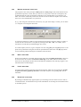
7.1.10
"Print and export" menu item
You can select your output format in a dialogue box. You have the following possibilities:
• "Printer"
allows graphic output of the current screen to the WINDOWS standard printer or to any
other printer selected using the menu item "File/Printer preferences". But you may also
select a different printer in the following dialogue box by pressing the "Printer
prefs./change printer" button.
In the upper group box, the maximum dimensions which the printer can accept are given.
Below this, the dimensions of the image to be printed are given. If the image is larger than
the output format of the printer, the image will be printed to several pages (in the above example, 4). In order to facilitate better re-connection of the images, the possibility of entering an overlap for each page, in x and y direction, is given. Alternatively, you also have
the possibility of selecting a smaller zoom factor, ensuring output to one page ("Fit to page" button). Following this, you can enlarge to the original format on a copying machine,
to ensure true scaling. Furthermore, you may enter the number of copies to be printed..
• "DXF file"
allows output of the graphics to a DXF file. DXF is a common file format for transferring
graphics between a variety of applications.
• "GGUCAD file"
allows output of the graphics to a file, in order to enable further processing with the
GGUCAD program. Compared to output as a DXF file this has the advantage that no loss
of colour quality occurs during export.
GGU-SLUGTEST User Manual
Page 21 of 71
September 2008
• "Clipboard"
The graphics are copied to the WINDOWS clipboard. From there, they can be imported
into other WINDOWS programs for further processing, e.g. into a word processor. In order
to import into any other WINDOWS program you must generally use the "Edit/Paste"
function of the respective application.
• "Metafile"
allows output of the graphics to a file in order to be further processed with third party software. Output is in the standardised EMF format (Enhanced Metafile format). Use of the
Metafile format guarantees the best possible quality when transferring graphics.
If you select the "Copy/print area" tool
from the toolbar, you can copy parts of
the graphics to the clipboard or save them to an EMF file. Alternatively you can send
the marked area directly to your printer.
Using the "Mini-CAD" program module you can also import EMF files generated using other GGU applications into your graphics.
• "MiniCAD"
allows export of the graphics to a file in order to enable importing to different GGU applications with the MiniCAD module.
• "GGUMiniCAD"
allows export of the graphics to a file in order to enable processing in the GGUMiniCAD
program.
• "Cancel"
Printing is cancelled.
GGU-SLUGTEST User Manual
Page 22 of 71
September 2008
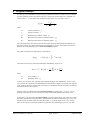
7.1.11
"Batch print" menu item
If you would like to print several appendices at once, select this menu item. You will see the following dialogue box:
Create a list of files for printing using "Add" and selecting the desired files. The number of files is
displayed in the dialogue box header. Using "Delete" you can mark and delete selected individual
files from the list. After selecting the "Delete all" button, you can compile a new list. Selection of
the desired printer and printer preferences is achieved by pressing the "Printer" button.
You then start printing by using the "Print" button. In the dialogue box which then appears you
can select further preferences for printer output such as, e.g., the number of copies. These preferences will be applied to all files in the list.
7.1.12
"Exit" menu item
After a confirmation prompt, you can exit the program.
7.1.13
"1, 2, 3, 4" menu items
The "1, 2, 3, 4" menu items show the last four files worked on. By selecting one of these menu
items the listed file will be loaded. If you have saved files in any other folder than the program
folder, you can save yourself the occasionally onerous rummaging through various sub-folders.
GGU-SLUGTEST User Manual
Page 23 of 71
September 2008
7.2
7.2.1
Edit menu
"Test data" menu item
Enter the principal test data required for slug test evaluation.
If your dataset contains the pure elevations above the at-rest groundwater level, enter 0 for
the initial water level.
7.2.2
"At-rest groundwater" menu item
Whilst processing the at-rest groundwater level, you can take into consideration that the at-rest
groundwater level fluctuates during a slug test. To make this practicable, data must be available
form relatively close observation gauges.
First, enter the number of value pairs you need to enter using "x points to edit". In the list that
follows this you can enter the time and corresponding groundwater level.
The individual values are then connected to a polygon. The program automatically takes these
changes in the at-rest groundwater level into consideration when evaluating the slug test.
GGU-SLUGTEST User Manual
Page 24 of 71
September 2008
7.2.3
"Equivalent radius" menu item
Normally, we assume for a slug test that the water level fluctuates in the region of the blank casing. However, there is one exception when the at-rest water level is within the region of the screen
or the filter gravel. The porosity of the filter gravel must then be taken into consideration. Together with the well development details, a new, so-called equivalent radius results in accordance
with
rc neu =
(1 − n ) rc2 + n rw2
where n is the porosity of the filter gravel.
If this configuration corresponds to that of the test you are evaluating, enter the porosity "neff" of
the filter material using this menu item. This input must be as a decimal, not a percentage!
You can view the new value for the casing radius rc by pressing the "Determine equiv. radius"
button.
If you would like to evaluate your test using the equivalent radius, click "As new radius". The
newly determined equivalent casing radius is then used in the test data. If you click the "OK"
button the value is not accepted and then serves information purposes only.
GGU-SLUGTEST User Manual
Page 25 of 71
September 2008
7.2.4
"Test designations" menu item
You can annotate the output sheet with additional, descriptive information concerning the test
being evaluated. Just enter the required data into the following dialogue box.
The texts in the input boxes in this dialogue box can be edited in Section 0 using the menu item
"Graphics preferences / Output preferences".
7.2.5
"Edit values" menu item
You can edit your measured data in a dialogue box.
• "Forw.", "Back"
If you have more than 10 value pairs you can navigate through them using these buttons.
• "Go to no.:"
You can advance to the specified value pair.
GGU-SLUGTEST User Manual
Page 26 of 71
September 2008
• "54 values to edit"
In the example shown here there are 54 value pairs. By pressing this button a dialogue box
opens in which the number of value pairs can be edited.
If no values are present (new test), the box will contain a 0. Value pairs can be appended
by increasing the number; by reducing the number, existing value pairs can be deleted from
the end of the list.
To delete pairs from an existing list, enter a time that is greater than the greatest actual
time.
The "Sort" button moves this line to the end of the list and it can then be deleted by appropriately reducing the number of values.
• "Sort"
If you have appended value pairs using the previously described button, you can have the
values correctly sorted by time using this button.
• "Cancel" or "OK"
You will leave the dialogue box without accepting the changes.
7.2.6
"Graphically" menu item
You can comfortably edit the imported data graphically on the screen. This saves a lot of time and
tedious typing or correcting of numbers. You can also view the changes in the graph immediately
on the screen. First, select the required action:
• "Move values"
Move the required data point by drag and drop using the left mouse button. The last move
can be undone by pressing the [Backspace] key.
• "Set/delete values"
Set a new point by clicking the left mouse button at the desired position.
An existing point is deleted by clicking it with the right mouse button. The last delete can
be undone by simultaneously pressing the [Backspace] and [Alt] keys.
GGU-SLUGTEST User Manual
Page 27 of 71
September 2008
7.2.7
"Modify" menu item
This menu item offers numerous options for processing your data.
These actions directly alter your measured data. No "undo" is available for any actions
with the exception of "Edit times" and "Edit measured values", i.e. you cannot reset any
of the editing performed on the data.
Before you carry out any irreversible manipulations on your data, you should save the file
under a different name in order to retain the original data.
• "Edit times"
By linking to a constant, you can convert the times associated with your values, e.g. from
[seconds] to [minutes].
• "Edit measured values"
You can edit your values by linking to a constant. This makes it very simple to correct
reading errors for all values.
GGU-SLUGTEST User Manual
Page 28 of 71
September 2008
• "Remove measured values"
You can decrease the number of values by deleting every nth value. This kind of data reduction is recommended for particularly large datasets, where the evaluation would otherwise
be extremely time intensive.
• "Double measured values"
If the number of values is very small, you can append a new value between two existing
ones. This is done by means of linear interpolation.
• "Values monotonous decreasing"
The values can be arranged monotonous decreasing.
• "Values monotonous increasing"
The values can be arranged monotonous increasing.
• "On Bezier curve method 1"
You can connect the data points with the help of a Bezier spline curve. The algorithm employed here adheres strictly to the data points (= method 1). The number of data points to
be considered for the curve can be entered in a dialogue box.
• "On Bezier curve method 2"
The data points are connected by a Bezier spline, whereby the curve is smoothed out
(= method 2). You enter the number of values to be used, just as in the previous action.
• "Values on a spline (!!!!)"
You can arrange the data points on a spline curve. After using this action a dialogue box
opens, in which you can specify the number of values to be included.
The weighting factor entered here influences the curve smoothing. The smaller the weighting, the smoother the curve.
GGU-SLUGTEST User Manual
Page 29 of 71
September 2008
• "Smooth values using spline"
With the help of this action you can generate an orderly, evaluatable curve from noisy data
using a compensation spline. A dialogue box opens, in which you specify the data points to
be included as model points.
Depending on the precise condition of the dataset you must select a more or less large separation of the model points to achieve a relatively smooth curve.
• "Roughen values"
This point was included to facilitate testing of the smoothing out methods described above.
For example, if you have simulated a slug test according to your specifications using the
"Test design" menu, i.e. calculated the data for a given permeability, you can make these
data noisy by any figure. Enter a maximum roughening value in metres into the dialogue
box and specify whether the roughening is proportional to the respective measured value.
• "OK"
You will leave the menu item.
7.2.8
"Value range "manually"" menu item
You can define ranges to be taken into consideration, or represented, for both the screen presentation and for your evaluation. If, for example, your dataset contains data from a slug and bail test,
you can select either the slug or the bail test for evaluation using this menu item. This function can
also be accessed using the [F7] key.
GGU-SLUGTEST User Manual
Page 30 of 71
September 2008
In the dialogue box you will see the minimum and maximum values for times and values automatically determined by the program for the representation range. For the evaluation range you
will see times only. You can enter your own values into the corresponding input boxes and thus
redefine the representation and evaluation ranges.
The program compares your times for the evaluation range with those for the existing data
points. For the "from" time, the value of the next lowest data point is used and for the "to"
time that of the next highest data point.
The times for the evaluation range must always form a subset of the times for the representation range. You will otherwise see a warning message and the times for the evaluation
range will be automatically adjusted by the program.
You can also redefine the evaluation range only to achieve the optimum screen display, using the
"Edit / Fit in" menu item (see Section 7.2.10).
7.2.9
"All" menu item
If you have altered the presentation on the output sheet using "Edit / Value range "manually"",
"Edit / Fit in" or "Edit / Graphically", this menu item will take you back to a presentation that
includes all measured values with the automatically determined minimum and maximum time and
height values. This function can also be accessed using the [F8] key.
7.2.10
"Fit in" menu item
The range selected using the "Edit / Value range "manually"" menu item is displayed using the
space available on the output sheet to its optimum. This function can also be accessed using the
[F9] key.
7.2.11
"Graphically" menu item
In principal, this is the same option as described in Section 7.2.8, the difference being that you can
comfortably define the value range graphically. All you have to do is simultaneously hold the
[Shift] and [Ctrl] keys together with the left mouse button to define the required window.
If you activate the check box "Apply to time axis only" in the message box, only the new time
coordinates are accepted; the y-axis with the height data remains unchanged (the diagram is
stretched in x-direction).
GGU-SLUGTEST User Manual
Page 31 of 71
September 2008
7.2.12
"General" menu item
You can annotate the output sheet with general information on the evaluated test. Enter the information into the following dialogue box.
Some of the texts in front of the input boxes can be edited in Section 0, using the menu item
"Graphics preferences / Output preferences", e.g. "Processed by:" and "Date:".
7.2.13
"Result text" menu item
At the bottom right of the output sheet a text box contains the results of the evaluation or simulation. The program default result text (see Section 7.3.6, menu item "Hvorslev, ... / Permeability")
can be edited and complemented in a total of 6 lines of input in the dialogue box.
7.2.14
"Company" menu item
In the top left box of the output sheet you can display your company's name and address in 4 lines
of text. Input is by means of the corresponding dialogue box. The information then appears centred in the text box.
If you would like to include company logos use the Mini-CAD module (see Section 7.6.10 and the
"Mini-CAD" manual).
GGU-SLUGTEST User Manual
Page 32 of 71
September 2008
7.3
7.3.1
Hvorslev, ... menu
"Height log" menu item
Use this menu item to display the y-axis (height) logarithmically.
Select this option if you would like to check whether your data approximately adhere to a descending e-function. With a logarithmic y-axis the result should be a straight line.
7.3.2
"Hvorslev" menu item
You can evaluate your slug test using the HVORSLEV (1951) method. However, you should have
first defined your preferences for this evaluation method as described in the next menu item.
A linear data curve appears on the screen. In addition, after selecting this menu item, the best-fit
curve (e-function) is drawn using the HVORSLEV (1951) model approach. After pressing [F12]
you will see the result of the evaluation for the best-fit curve.
You can achieve a clear presentation of the data curve and the best-fit curve by going to the
menu items "Graphic preferences / Preferences" and "Graphic preferences / Pen colour
and width" (Sections 7.6.1 and 0) and specifying presentation preferences.
7.3.3
"(Hvorslev) - preferences" menu item
If you want to evaluate using the HVORSLEV method, you must first select an evaluation equation
after HVORSLEV to suit your problem. In the dialogue box which then opens, you are presented
with the well configurations. The variable head method after HVORSLEV is implemented in the
program.
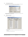
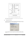
Case A applies to a perfect well in a free aquifer. Case B applies to a perfect well in a confined
aquifer.
GGU-SLUGTEST User Manual
Page 33 of 71
September 2008
Figure 1: Well configurations for HVORSLEV evaluation
In addition, you can enter a value to represent the ratio of horizontal to vertical permeability. Internally, the program uses the root of this ratio. This allows due consideration of anisotropy.
After confirming your input with "OK" you will be automatically presented with the data and
best-fit curves after HVORSLEV.
7.3.4
"Bouwer + Rice" menu item
This menu item allows you to adopt the evaluation method after BOUWER & RICE (1976). However, you should have first defined your preferences for this evaluation method as described in the
next menu item.
The best-fit curve (e-function) is drawn beside the data curve using the BOUWER & RICE model
approach. After pressing [F12] you will see the result of the evaluation for the best-fit curve.
You can achieve a clear presentation of the data curve and the best-fit curve by going to the
menu items "Graphic preferences / Preferences" and "Graphic preferences / Pen colour
and width" (Sections 7.6.1 and 0) and specifying presentation preferences.
GGU-SLUGTEST User Manual
Page 34 of 71
September 2008
7.3.5
"(Bouwer + Rice) - preferences" menu item
For an evaluation after BOUWER & RICE you must also first select a well configuration to suit
your problem from the following dialogue box.
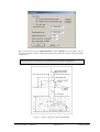
You can choose from an imperfect well (Case A) and a perfect well (Case B). The BOUWER &
RICE evaluation model can be adopted for both a free and a (semi-) confined aquifer.
You must then enter the distance between the groundwater table (at-rest water level) and the base
of the well (well toe), and the thickness of the layer filled by the groundwater.
The depth of the groundwater must always be greater than the distance between the well
toe and the groundwater table.
GGU-SLUGTEST User Manual
Page 35 of 71
September 2008
Figure 2: Well configuration for BOUWER & RICE evaluation
After confirming your input with "OK" you will be automatically presented with the data and
best-fit curves after BOUWER & RICE.
7.3.6
"Permeability" menu item
In order to get a result from an evaluation after HVORSLEV or BOUWER & RICE, you must go to
this menu item after selecting one of the two methods and defining your preferences. A small text
window then opens, containing the principal evaluation results.
The first line indicates the evaluation method with the corresponding well and aquifer configuration. For HVORSLEV, kf then follows, together with the correlation coefficient and the calculated
e-function.
GGU-SLUGTEST User Manual
Page 36 of 71
September 2008
For the evaluation after BOUWER & RICE, kf is followed by the transmissivity and then the parameter C. This parameter is required internally for the calculation of certain quantities involved in
the BOUWER model and is intended as a control mechanism for advanced users.
The range of the slug tests follows this. Finally, the equation for the adapted e-function is given,
followed by the correlation coefficient as a measure of the agreement between the measured data
and the calculated course.
You confirm the results with "OK" and close the result window. The "As result text" button
sends the content of the result window to your output sheet. The complete text then appears in the
lower right box of the output sheet. The text can be processed further using the "Edit / Result
text" menu item (see Section 7.2.13).
7.3.7
"Individual values" menu item
Use this menu item to study a point on your curve in more detail. Click on the data point with the
left mouse button. A message window opens, as shown in the following example for point no.
415. Close the window using the "OK" button.
GGU-SLUGTEST User Manual
Page 37 of 71
September 2008
7.4
Type curves menu
The GGU-SLUGTEST program allows the evaluation of slug tests employing the model approaches after COOPER et al.(1967), DOUGHERTY (1989), MATEEN (1983), RAMEY et al.
(1975) and MOENCH & HSIEH (1985 a).
7.4.1
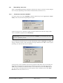
"Cooper" / "Ramey" / "Dougherty" / "Mönch" menu item
In the program's default setting, the first menu item in the "Type curves" menu is "Cooper". Select the required model here, as shown in the following dialogue box. The name of the menu item
will be adjusted in the further course of the program, depending on the model selected, e.g. "Type curves / Ramey".
When selecting a model, the well geometry, the aquifer configuration and the data itself should be
taken into consideration.
You can select from:
• COOPER (perfect well with wellbore storage in a homogeneous, isotropic, confined aquifer)
• DOUGHERTY (imperfect well with wellbore storage in a homogeneous, isotropic, confined aquifer)
• RAMEY (perfect well with wellbore storage and infinite skin in a homogeneous, isotropic,
confined aquifer)
• MOENCH (perfect well with wellbore storage and finite skin in a homogeneous, isotropic,
confined aquifer)
In addition, you can choose to have the test evaluated by means of normal type curves or the derivative of the type curves.
The evaluation by means of the type curve derivative makes sense if you want to
perform a "hand fit".
If the type curves are represented as derivatives, they are generally easier to differentiate from one
another than the normal representation. This helps when selecting by hand the best-fitting derivative and thus the type curve.
GGU-SLUGTEST User Manual
Page 38 of 71
September 2008
The name of the following menu item is adjusted according to the selected test evaluation, e.g.
"Type curves / Cooper preferences".
Confirm the model selection and test evaluation using "OK". If you have already loaded a dataset,
the standard type curves are presented on the output sheet corresponding to the evaluation models
and your data curve.
7.4.2
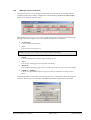
"Cooper preferences" / "Derivative preferences" menu item
This menu item applies equally to the model approaches after RAMEY, DOUGHERTY and
MOENCH, and the derivatives of the various type curves.
A dialogue window for defining H0 preferences opens when you go to this menu item.
You can select:
• the first value of your selected measurement range,
• the maximum of the measurement range or
• any fixed value.
The "To fixed" buttons allow you to assign the first value or the greatest value of the measurement
range as fixed H0. The value is then transferred to the input box.
Please note that H0 has a decisive influence on the curvature of the data, particularly
at the start of the curve, because in a COOPER graph the quotient H/H0 is represented.
The value chosen for H0 can therefore have a critical influence on your result.
In the dialogue box above you can also define a displacement factor (> 0!) for the data curve.
Initially, a factor of 1 is shown for the undisplaced curve. By horizontal displacement along the
time axis the data curve is brought to congruence with the best fitting type curve. The displacement factor is used in the calculation of the transmissivity and permeability.
GGU-SLUGTEST User Manual
Page 39 of 71
September 2008
Your input is accepted after you leave the dialogue box via the "OK" button and the adapted representation drawn on the worksheet.
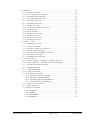
In the following figure the model approach after COOPER is shown with the relevant parameters.
Figure 3: Aquifer configuration after COOPER
If you have chosen "DOUGHERTY" (the same as COOPER, but for an imperfect well) as
evaluation model, you will see an expanded dialogue box.
GGU-SLUGTEST User Manual
Page 40 of 71
September 2008
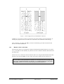
Here, you must also enter the "Aquifer thickness" and the "Distance" (base of aquifer - base of
screen)" (see Figure 4: UKAq - UKF). This information is required to produce a pertinent model
configuration.
This means that new values must be entered for each new aquifer configuration.
Figure 4: Aquifer configuration after DOUGHERTY
GGU-SLUGTEST User Manual
Page 41 of 71
September 2008
The "RAMEY" evaluation model corresponds to the configuration of the COOPER model (see
Figure 3, Page 40).
For the "MOENCH" evaluation model, which includes a finite skin zone around the well, you
must additionally enter
• the ratio of the permeabilities of the aquifer to the skin zone,
• the ratio of the storage coefficient of the skin zone to the aquifer and
• a radius for the skin zone.
Figure 5: Aquifer configuration after MOENCH
7.4.3
"Derivative preferences" menu item
If you have decided on an evaluation by means of the derived type curves you can define the following parameters using this menu item:
• a scaling factor for the y-axis (h/H0) for the data curve and the derived type curve and
• a displacement factor for the derived data curve in the x-direction (time axis).
GGU-SLUGTEST User Manual
Page 42 of 71
September 2008
7.4.4
"Hand fit" menu item
For an initial overview it is often sufficient to evaluate by hand. "Hand fit" allows you to bring
the data curve to congruence with one of the type curves using the mouse. Before doing this you
must specify from which value the curve is displaced. A small dialogue window opens.
Data curve displacement is faster the greater the selected "Delta value". You will have to show a
little patience for especially large datasets.
As long as you hold the left mouse button the data curve can be horizontally displaced by any
amount.
Take note of the status bar: kf is shown here in real time.
This will help to give you a feeling for how the permeability varies for a "fit" from type
curve to type curve.
7.4.5
"Autofit 1" menu item
If the "Type curves / Autofit 1" menu item is selected the program automatically compares the
data with the existing type curves and searches for the best fitting type curve using the least
squares method.
Please ensure that you do not have only a very few type curves in your type curves file, because the program will always find a type curve that fits best.
Before you can perform an "Autofit 1" you must specify in a dialogue window which nth data
points of the data curve are to be compared to the type curves. Normally, you can work with the
default setting "x = 1", i.e. every data point is included in the comparison. You can reduce the
number of data points for very large datasets, by entering 10, for example. This makes things a
little faster.
GGU-SLUGTEST User Manual
Page 43 of 71
September 2008
In addition, you can specify the range for H/H0, that is, the region of the y-axis for which the fit is
performed. The default range is from 0.02 to 0.98. The data often become noisy towards the end
of a measuring campaign. This area can also be blanked out.
Confirm your input using the "OK" button. The program then searches without further ado for the
best fitting type curve.
When the analysis is complete a window opens displaying the selected type curve parameter for
your evaluation model. The maximum absolute deviation between the data curve and the type
curve is calculated for this purpose. If you close the window with "OK", the type curve fit is
drawn on the worksheet.
If, on the other hand, you press the "As only TCM" button, only the best fitting type curve is
drawn on the worksheet with the data curve. Any existing type curves will be deleted.
When employing the "DOUGHERTY" and "MOENCH" models you must ensure that
you really have generated the type curves most suitable for your aquifer and well geometry,
using the menu item "Type curves / Generate" (see Section 7.4.10).
If the type curves do not fit your geometry you will see an error message; you should not
ignore this. Otherwise you will begin an evaluation with type curves unsuitable for your
current configuration and the results may well be nonsense.
GGU-SLUGTEST User Manual
Page 44 of 71
September 2008
7.4.6
"Autofit 2" menu item
Using this fit method, the best fitting type curve is not selected from an existing set of type curves,
but the optimum type curve is calculated. This means that the program generates the optimum fit
type curve by systematic variation of the type curve parameter. If you have decided on "Autofit 2"
the following dialogue box opens:
In the dialogue box you can specify which nth data points of the data curve are considered for
"Autofit 2". Here, once again, you can limit the range of H/H0. Moreover, you can define a minimum and a maximum type curve parameter, between which the type curve parameter varies. You
must also specify a surcharge factor for the type curve parameter. Do not make this factor too
small at first, or go for a coffee afterwards.....
Finally, you have the option of notifying the program whether to accept the newly calculated,
optimum type curve. If you activate this check box, the existing type curves are deleted.
Once you have specified all preferences and concluded input with "OK", a further dialogue box
opens with the heading "Type curve generator after Cooper" (the name corresponds to the
evaluation model selected).
GGU-SLUGTEST User Manual
Page 45 of 71
September 2008
Because a type curve is calculated by means of the Stehfest algorithm, you can edit the number of
Stehfest weighting factors here. In principle, the calculation of a type curve is more precise the
more Stehfest points (even number!) are used. However, computing time also increases with an
increase in the number of Stehfest points. The program achieves good results with 8,10,12,14,16
and 18 Stehfest points. You should generally leave this at 12 points. Nevertheless, it is still possible that given parameter combinations, in conjunction with a given number of Stehfest points, may
lead to an unrealistic type curve.
In addition, you can specify the start ("Min beta") and end time ("Max beta"), and the number of
times per logarithmic decade for the optimised type curve. If these parameters are cleverly selected
the computation time can be greatly reduced.
With regard to the times, please note that these are dimensionless type curve times.
Once you have entered all the required values, close the window with "OK" and "Autofit 2" finds
an optimum type curve. You can follow the variation of the type curve parameter in the status bar.
After computation of the optimum type curve an info box opens showing the found optimum type
curve parameter and the maximum absolute deviation between the type curve and the measured
data. After confirming with "OK" you are asked whether the type curve parameter should be further delineated.
If you answer "No" then "Autofit 2" is complete and you see the type curves on your worksheet.
If you answer the question with "Yes", you will next see the following info box; close it by clicking "OK".
The program now offers you the opportunity of defining all required parameters. Generally, you
should simply leave the values proposed automatically by the program. However, you are free to
enter your own values. In this manner you can further delineate the type curve parameters in several computation runs.
Ensure that the maximum absolute deviation between the type curve and the measured data
really does decrease.
GGU-SLUGTEST User Manual
Page 46 of 71
September 2008
7.4.7
"Permeability" menu item
After a completed fit the hydraulic parameters derived from it will be of interest. Various dialogue
boxes will open, depending on the evaluation model selected (see Section 7.4.1).
7.4.7.1
Evaluation model after COOPER
If you have chosen to use the "COOPER" evaluation model and go to the "Type curves / Permeability" menu item, the following dialogue box opens:
In this box the type curve parameter, together with the well data from which the storage coefficient is calculated, is proposed for an automatic fit.
ATTENTION: If you have previously performed a "hand fit", you must enter the correct
type curve parameter yourself.
If you confirm the proposed value or the value determined by means of "hand fit" with "OK", the
storage coefficient is shown. After confirming the storage coefficient with "OK" a new box opens,
presenting you with the result of your evaluation.
In the first line you are reminded of the selected evaluation model. Below this are kf and the userdefined H0, the transmissivity and the storage coefficient once again. Close this info box with
"OK". If you would like to transfer the results to your worksheet, click the "As result text" button. The results are then displayed in the lower right box of the worksheet (also see the "Edit /
Result text" menu item, Section 7.2.13).
GGU-SLUGTEST User Manual
Page 47 of 71
September 2008
7.4.7.2
Evaluation model after RAMEY
If you selected the "RAMEY" model for your fit and you activate the "Type curves / Permeability" menu item, a window opens with the heading "Determine storage coefficient or skin" and
showing the type curve parameters and the storage coefficient. Furthermore, a value for the skin is
proposed.
Because the RAMEY method can calculate either only the storage coefficient or only the skin, one
of the two variables must already be known in order to calculate the other. You therefore have the
option of having either the storage coefficient calculated for a user-defined skin value or having
the skin calculated for an estimated storage coefficient. When you have done this a small window
opens displaying the values.
In addition, the hydraulically effective well radius is calculated from the skin and displayed here.
If you confirm the values with "OK" a new window opens with the heading "Type curves after
Ramey", showing all evaluation results.
These results consist of the permeability kf, the initial height H0, the transmissivity, the storage
coefficient, the skin and the effective well radius. If desired, you can use this result as the result
text in the lower right box of the worksheet.
GGU-SLUGTEST User Manual
Page 48 of 71
September 2008
7.4.7.3
Evaluation model after DOUGHERTY
Using the "DOUGHERTY" model, the type curve parameter is displayed in a "Determine storage coefficient" dialogue box.
You can accept this parameter for the autofits.
ATTENTION: If you have previously performed a "hand fit", you must enter the correct
type curve parameter yourself.
If you confirm the proposed value or the value determined by means of "hand fit" with "OK", the
storage coefficient is shown. After confirming the storage coefficient with "OK" a "Type curves
after Dougherty" result window opens with all relevant evaluation values.
If required, the contents of the result window can be transferred to the worksheet. This is done by
pressing the "As result text" button.
7.4.7.4
Evaluation model after MOENCH
The "MOENCH" model applies accordingly. A type curve parameter for calculation of the storage coefficient is proposed. Following a hand-fit you must enter the correct type curve parameter
yourself.
Once you have accepted or entered the value, click on "OK" and the storage coefficient will be
displayed. Another click on "OK" opens a window with the heading "Type curves after Mönch".
Here, you can see all evaluation parameters, such as kf, H0, the transmissivity and the storage
coefficient. Furthermore, the user-defined ratios of aquifer permeability to skin zone permeability
and skin storage coefficient to aquifer storage coefficient, and the ratio of skin radius to well radius, are given. If required, the contents of the result window can be transferred to the worksheet
using the "As result text" button.
GGU-SLUGTEST User Manual
Page 49 of 71
September 2008
7.4.8
"Edit type curves" menu item
Using this menu item you can manage the type curves in the system for the currently selected
evaluation model. After clicking, a dialogue box with the heading "Type curves after Cooper",
similar to the following example, opens.
There are already seven type curves in this example. The buttons are automatically labelled with
the alpha value of the respective type curve. The following actions are possible:
• "To menu bar"
You will return to the menu bar
• "New"
You can enter a new type curve.
NOTE: New type curves cannot be calculated using this menu item!
• "Load"
You can load a dataset with previously saved type curves.
• "Save"
You can save existing type curves together in a dataset.
• "Delete all"
You can delete all existing type curves, in order to generate new type curves, for example.
• "1.000E-6", "1.000E-5", .....
You can view and edit the respective type curve data, if required, by clicking on each
button.
After clicking "New", or the button of an existing type curve, a dialogue box opens allowing you
to enter or edit the type curve parameter and additional parameters, depending on the model.
GGU-SLUGTEST User Manual
Page 50 of 71
September 2008
This allows you to append new type curves acquired, for instance, by copying from publications
or other sources. If you choose "New" but close the box using "Cancel", any alterations made will
be rejected, but the type curve itself will be retained (new button with the alpha value labelling).
Individual curves can be deleted using the "Delete type curve" button.
If you clicked the "Edit type curve values" button, you can enter or edit individual type curve
values in a dialogue box. In the title bar of the dialogue box the evaluation model is shown and, in
brackets, the type curve parameter of the selected type curve.
No points exist for a new type curve. First, click on the "0 points to edit" button (in the example
above 71 points already exist) and enter the required number. You can navigate through the list
using "Forw." and "Back" or jump directly to the required point by entering the number and clicking "Go to no.:" To conclude your entry or edit click "Done".
GGU-SLUGTEST User Manual
Page 51 of 71
September 2008
7.4.9
"Select" menu item
Using this menu item you have the option of comfortably selecting any type curves for representation.
Activate the check boxes in front of the required type curves. You can quickly select "All" or
"None" with the corresponding buttons. After selection, close the dialogue box with "OK".
In order to make the type curves appear on the worksheet, press either [Esc] or [F2] after
selecting them and closing the box.
7.4.10
"Generate" menu item
The type curve generator can generate any number of type curves for the models COOPER,
DOUGHERTY, RAMEY and MOENCH. You can define the respective parameters according to
your own requirements. However, you should be aware of which parameter combinations are
sensible and which are not.
The models COOPER and RAMEY are universal models: beside the type curve parameters, no
other data is utilised for the calculation.
The models DOUGHERTY and MOENCH are special models. This means that the type curves are
valid only for special aquifer and well geometries.
GGU-SLUGTEST User Manual
Page 52 of 71
September 2008
7.4.10.1
COOPER
A dialogue box with the heading "Type curve generator after Cooper" opens.
First, you enter the "Number of Stehfest points". This correlates directly to the numerical method
used for calculating the type curves. Generally, you should leave this at the 12 point default. In
principle, however, the type curve would be more precise the higher the number of Stehfest model
points. Nonetheless, because of the limited precision of your computer, the results may be rather
strange for values above 18.
The number of Stehfest points must always be even.
Next, you enter the type curve parameter alpha. A useful range here is between 1e-1 and 1e-10,
approximately. You can now enter the dimensionless start and end time for the type curve. A useful range for beta here is between 1e-4 und 1e+4. Finally, you are asked for the number of time
steps per logarithmic decade. The default value is ten steps.
The higher the number of steps, the greater the number of values pairs included in the type
curve. The computation time increases accordingly.
Once you have defined everything as you require, confirm your input with "OK", or abort the
process with "Cancel".
When the program has concluded computations you are asked whether you want to save the type
curve. If you answer this by pressing the "Yes" button a Windows dialogue box opens where you
can use "Save file as" to save the type curve. The program suggests ".tku" as the extension for the
type curve file name.
If you have saved the type curves or replied to the previous question with "No", you will be asked
whether the type curve should be included in the list of available curves. The program then stores
the curve.
If you want the calculated type curves to be permanently saved, you must save them using "Type
curves / Edit type curves" button "Save", as described in Section 7.4.8. The default file is called
"GGU-SLUGTEST.tkv".
GGU-SLUGTEST User Manual
Page 53 of 71
September 2008
7.4.10.2
RAMEY
In principle, generating type curves according to the Ramey evaluation model is exactly the same
as the COOPER model. The only difference for Ramey is the type curve parameter CD e2s.
GGU-SLUGTEST User Manual
Page 54 of 71
September 2008
7.4.10.3
DOUGHERTY
In the DOUGHERTY model you must know the well and aquifer geometry, beside input of the
previously mentioned parameters, or at least enter plausible estimates. You should have the following parameters ready:
• the aquifer thickness,
• the distance between the base of the aquifer and the base of the screen,
• the distance between the base and the top of the screen (length of screen).
These values must be respectively divided by the borehole radius.
The information corresponds to the information entered in the menu item "Edit / Test data" (see
Section 7.2.1). So you see, the type curves for an imperfect well after DOUGHERTY are precisely
adapted to your respective system.
You then enter the start and end time (dimensionless type curve time) and the number of times per
decade.
When you are ready to start the computation click "OK". The computation may take some time if
you have a slow computer.
Once the computation is complete you can once again decide whether the type curve should be
saved and/or placed in the list of available curves.
GGU-SLUGTEST User Manual
Page 55 of 71
September 2008
7.4.10.4
MOENCH
In contrast to the RAMEY model, the model approach after MOENCH takes into consideration a
skin zone of limited extent around the well (finite skin). Accordingly, this skin zone possesses a
radius (measured from the borehole centre), a permeability and a storage coefficient.
Beside the Stehfest points and the type curve parameters, you must tell the program
• the ratio of the permeability of the aquifer to the permeability of the skin zone,
• the ratio of the storage coefficient of the skin zone to the storage coefficient of the aquifer
and
• the ratio of the radius of the skin zone to that of the borehole or the well
.
Here, too, it is advisable to carefully consider the configuration for the type curve calculation. For
example, for a well in a relatively impermeable rock, the permeable filter gravel fill can be taken
into consideration as a skin zone.
All further steps have already been described.
GGU-SLUGTEST User Manual
Page 56 of 71
September 2008
7.5
7.5.1
Test design menu
General note for the Test design menu
This menu allows the simulation of a slug test for all implemented models.
This is particularly useful for planning upcoming tests. You should use this option extensively in
order to acquire a feel for the possible changes in water levels for varying aquifer and well types.
7.5.2
"Hvorslev" menu item
After selecting this item a "Test design after Hvorslev" dialogue box opens. The same configuration (Case A/B) appears that you previously selected in the menu item "Hvorslev /
- preferences" (see Section 7.3.3).
Enter an estimate for the permeability in the dialogue box. In addition, you must enter a water
level at the start of the test (the increase for a slug test) and the end of the test. Finally, you can
enter the number of data pairs ("No. of values =") for the simulated curve.
Well data input is carried out via the menu item "Edit / Test data" (see Section 7.2.1).
After confirming the data with "OK", the data graph is immediately displayed on your worksheet
according to the HVORSLEV model.
GGU-SLUGTEST User Manual
Page 57 of 71
September 2008
7.5.3
"Bouwer + Rice" menu item
You will see the same dialogue box as in the previous menu item, but with a different heading.
Input is the same as for "Test design / Hvorslev".
7.5.4
"Cooper" / "Ramey" / "Dougherty" / "Mönch" menu item
The title of this menu item reflects the evaluation model selected in "Type curves / Cooper" (see
Section 7.4).
The "Test design after Cooper" dialogue window that opens when "COOPER" is selected asks
for the permeability and the storage coefficient. In addition, you can enter the increase for a fictitious test, as well as the water level at the end of the test. Finally, you enter the number of values
per logarithmic decade.
After confirming with "OK" a new dialogue box opens, where you enter the number of Stehfest
points. The type curve parameter alpha shown on the screen was determined by the program from
your well data (menu item "Edit / Test data", Section 7.2.1) and the storage coefficient.
You should not alter the type curve parameter alpha!
GGU-SLUGTEST User Manual
Page 58 of 71
September 2008
After confirmation with "OK" the simulated graph is displayed together with the COOPER type
curve.
"RAMEY" model: see Section 7.4.10.2 "Type curves / Generate" (RAMEY)
"DOUGHERTY" model: see Section 7.4.10.3 "Type curves / Generate" (DOUGHERTY)
"MOENCH" model: see Section 7.4.10.4 "Type curves / Generate" (MOENCH)
7.6
7.6.1
Graphic preferences menu
"Preferences" menu item
In a dialogue box you can define preferences and alter the appearance of the graph and the type
curves.
You can connect the data points to a curve and have the data points marked by a circle. The number and size of the markers can be specified at the bottom of the dialogue box.
By activating the appropriate check box you can display the regression curve (HVORSLEV,
BOUWER & RICE) in the graphics. You can also choose to display the at-rest water level.
If you wish to have the type curves annotated, activate the corresponding check box and, if necessary, enter a different text size. By activating the required dimension for the time axis the representation can be displayed in seconds, minutes, hours or days.
After confirming your input with "OK" the graph is redrawn according to your preferences.
GGU-SLUGTEST User Manual
Page 59 of 71
September 2008
7.6.2
"Refresh and zoom" menu item
The program works on the principle of What you see is what you get. This means that the screen
presentation represents, overall, what you will see on your printer. In the last consequence, this
would mean that the screen presentation would have to be refreshed after every alteration you
make. For reasons of efficiency and as this can take several seconds for complex screen contents,
the screen is not refreshed after every alteration.
If, e.g., after using the zoom function (see below), only part of the image is visible, you can achieve a complete view using this menu item.
A zoom factor between 0.4 and 8.0 can be entered in the input box. By then clicking on "Use" to
exit the box the current factor is accepted. By clicking on the "0.4", "0.6", etc. buttons, the selected factor is used directly and the dialogue box closed.
It is much simpler, however, to get a complete overview using [Esc]. Pressing [Esc] allows a complete screen presentation using the zoom factor specified in this menu item. The [F2] key allows
screen refreshing without altering the coordinates and zoom factor.
7.6.3
"Save" menu item
Some of the preferences you made with the menu items of the "Graphics preferences" menu can
be saved to a file. If you select "GGU-SLUGTEST.alg" as file name, and save the file on the
same level as the program, the data will be automatically loaded the next time the program is started and need not be entered again.
7.6.4
"Load" menu item
You can reload a graphics preferences file into the program, which was saved using the "Graphics preferences/Save graphics preferences" menu item. Only the corresponding data will be
refreshed.
7.6.5
"Zoom info" menu item
By clicking two diametrically opposed points you can enlarge a section of the screen in order to
view details better. An information box provides information on activating the zoom function and
on available options.
GGU-SLUGTEST User Manual
Page 60 of 71
September 2008
7.6.6
"Pen colour and width" menu item
You can edit the line widths and colours for selected elements.
A dialogue box is opened if you click on the "Standard", "Type curves", "Height", "GW zero"
or "Regression" buttons; here you can specify a colour as required. The preferences can be saved
in the "GGU-SLUGTEST.ALG" file.
If you use a monochrome (black and white) printer, you must select the colours as dark as
possible, otherwise it is possible you will see nothing on the printout.
7.6.7
"Legend font selection" menu item
With this menu item you can switch to a different true-type font. All available true-type fonts are
displayed in the dialogue box.
7.6.8
"Font sizes" menu item
You can edit font sizes of texts [in mm] within the various input areas.
GGU-SLUGTEST User Manual
Page 61 of 71
September 2008
7.6.9
"Output preferences" menu item
Using this menu item you can enter or edit the default text on your output sheet. If you save the
"GGU-SLUGTEST.ALG" file containing the preferences at the same level as the program, they
will be used automatically when the program is started.
If you would prefer to use the default settings, simply click the "Reset" button.
7.6.10
"Mini-CAD toolbar" menu item
Using this menu item you can add free text to the graphics and add lines, circles, polygons and
images (e.g. files in formats BMP, JPG, PSP, TIF, etc.) . A pop-up menu opens; the icons and
functions used are described in more detail in the "Mini-CAD" manual provided.
GGU-SLUGTEST User Manual
Page 62 of 71
September 2008
7.6.11
"Toolbar preferences" menu item
After starting the program a horizontal toolbar for menu items appears below the program menu
bar. If you would rather work with a popup window with several columns, you can specify your
preferences using this menu item. The smarticons can also be switched off.
At the bottom of the program window you find a status bar with further information. You can also
activate or switch off the status bar here. The preferences will be saved in the "GGUSLUGTEST.alg" file (see menu item "Graphics preferences/Save graphics preferences") and
will be active at the next time the program is started.
By clicking on the tools (smarticons) for menu items you can directly reach most of the program
functions. The meaning of the Smarticons appears as a text box if you hover with the mouse
pointer over the tools. Some of the tool functions can be activated from the normal menu items.
"Zoom out"
If you have previously zoomed in, this tool returns to a full screen display.
"Zoom (-)" /"Zoom (+)"
With the zoom functions you can zoom in or out of parts of the image, by clicking the left mouse
button.
"Copy/print area"
Use this tool to copy only parts of the graphics in order to paste them, e.g. to a report. You will see
information on this function and can then mark an area, which is copied to the clipboard or can be
saved in a file. Alternatively you can send the marked area directly to your printer.
"Colour on / off"
If you need to remove the colour from the system presentation, to create a black and white
printout, for example, use this on / off switch.
GGU-SLUGTEST User Manual
Page 63 of 71
September 2008
7.7
7.7.1
? menu
"Copyright" menu item
You will see a copyright message and information on the program version number.
The "System" button shows information on your computer configuration and the folders used by
GGU-SLUGTEST.
7.7.2
"Maxima" menu item
You will see information on the maximum values. allowed by the program
7.7.3
"GGU on the web" menu item
Using this menu item you can access the GGU Software website: www.ggu-software.com.
Keep in touch with new program versions and the regular download offers.
If you would like to be automatically notified about program innovations, please register for the
Newsletter in our Knowledge Base. Go to the following website: http://kbase.civilserve.com.
7.7.4
"GGU support" menu item
This menu item takes to the GGU-Software Support area at www.ggu-software.com.
7.7.5
"Help" menu item
The GGU-SLUGTEST online-help is opened using an installed browser (e.g. MS Internet Explorer). The help function can also be accessed using the [F1] function key.
7.7.6
"What's new?" menu item
You will see information on program improvements in comparison to older versions.
7.7.7
"Language preferences" menu item
This menu item allows you to switch the menus and the graphics from German to English and vice
versa. To work in German, deactivate the two switches "Dialoge + Menüs übersetzen (translate
dialogues, menus)" und "Graphiktexte übersetzen (translate graphics)".
Alternatively, you can work bilingually, e.g. with German dialogue boxes but with graphic output
in English. The program always starts with the language setting applicable when it was last ended.
GGU-SLUGTEST User Manual
Page 64 of 71
September 2008
8 Tips
8.1
Pressurised slug tests
When entering the test data for evaluation of so-called pressurised slug tests (pulse tests), the
casing radius rc must be replaced by:
rcneu = rc ⋅
l ⋅ cw ⋅ ρ w
where:
rc :
Casing radius [m]
l:
Test distance [m]
cw :
Compressibility of test zone [m2/N]
ρw :
Density of water [kg/m3]
If cw is not precisely known, calculations may be performed using the compressibility of water
instead (4.78 · 10-10 m2/N-1 at 10 °C).
8.2
Keyboard and mouse
You can scroll the screen with the keyboard using the cursor keys and the [Page up] and [Page
down] keys. By clicking and pulling with the mouse, with [Ctrl] pressed, you activate the zoom
function, i.e. the selected section will fill the screen. Furthermore you can use the mouse wheel to
zoom in/out or scrolling the screen presentation. The following mouse wheel functions are
available:
• Mouse wheel up
= move screen image up
• Mouse wheel down
= move screen image down
• [Ctrl] + mouse wheel up
= enlarge screen image (zoom in)
• [Ctrl] + mouse wheel down
= shrink screen image (zoom out)
• [Shift] + mouse wheel up
= move screen image right
• [Shift] + mouse wheel down
= move screen image left
By double-clicking the left mouse button on output sheet or Mini-CAD objects, the editor for the
selected object immediately opens, allowing it to be edited. By double-clicking output sheet elements while holding the [Shift] key, the preferences for the position, size and appearance of the
element open for editing in the editor.
GGU-SLUGTEST User Manual
Page 65 of 71
September 2008
Some of the function keys are assigned program functions. The allocations are noted after the
corresponding menu items. The individual function key allocations are:
• [Esc] refreshes the screen contents and sets the screen back to the given format. This is
useful, for example, if you have used the zoom function to display parts of the screen and
would like to quickly return to a complete overview.
• [F1] opens the menu item "Hvorslev, ... / Height log".
• [F2] refreshes the screen without altering the current magnification.
• [F3] opens the menu item "Hvorslev, ... / Hvorslev".
• [F4] opens the menu item "Type curves / Cooper (or similar)".
• [F5] opens the menu item "Type curves / Hand fit".
• [F6] opens the menu item "Hvorslev, ... / Bouwer + Rice".
• [F7] opens the menu item "Edit / Value range "manually"".
• [F8] opens the menu item "Edit / All".
• [F9] opens the menu item "Edit / Fit in".
• [F11] opens the menu item "Type curves / Autofit 1".
• [F12] opens the menu item "Hvorslev, ... / Permeability" or "Type curves /
Permeability".
GGU-SLUGTEST User Manual
Page 66 of 71
September 2008
9 Bibliography
BARKER, J.A. & BLACK, J.H. (1983): Slug tests in fissured aquifers.
Water Resources Research (19):6,1558-1564.
BOUWER, H. (1989): The Bouwer and Rice slug test - an update.
Ground Water (27):3,304-309.
BOUWER, H. & RICE, R.C. (1976): A slug test for determining hydraulic conductivity of
unconfined aquifers with completely or partially penetrating wells.
Water Resources Research (12):3,423-428.
BREDEHOEFT, J.D. & PAPADOPULOS, S.S. (1980): A method for determining the
hydraulic properties of tight formations. Water Resources Research (16):1,233-238.
COOPER, H.H. & PAPADOPULOS, J.D. BREDEHOEFT. I. S. (1967): Response of a finitediameter well to an instantaneous charge of water.
Water Resources Research (33):1,263-269.
DA PRAT, G. (1981): Well test analysis for naturally-fractured reservoirs.
Diss. Univ. Stanford, 202 S.
DA PRAT, G. (1990): Well test analysis for fractured reservoir evaluation.
In: Developments in Petroleum Science 27, CHILINGARIAN, G.V. (Ed.),
1st Ed., Elsevier, Amsterdam, 210 S.
DOUGHERTY, D.E. (1989): Computing well hydraulics solutions.
Ground Water (27):4,564-569.
EARLOUGHER, R.C. (1977): Advances in well test analysis.
AIME, SPE OF (Ed.), 2nd Ed., New York, Dallas, 259 p.
FAUST, CH.R. & MERCER, J.W. (1984): Evaluating of slug tests in wells containing a finitethickness skin. Water Resources Research (20):4,504-506.
FERRIS, J.G. & D.B. KNOWLES (1954): The slug test for estimating transmissivity.
U.S. Geol. Surv. Groundwater Note 26.
FLOPETROL (1983): Well test interpretation for monophasic oil by analysis of pressure
behavior. In: Systems Analysis Part 1,
SCHLUMBERGER, FLOPETROL (Ed.), Melun, France.
GRADER, A.S. & RAMEY, H.J. (1988): Slug-test analysis in double-porosity reservoirs.
SPE Formation Evaluation, June, 329-339.
GRINGARTEN, A.C. (1980): Well test interpretation.
Flopetrol Schlumberger 1.1-7.3.
HURST, W. (1953): Establishment of the skin effect and its impediment to fluid flow into a well
bore. The Petroleum Engineer 10, B6-B16.
HVORSLEV, M.J. (1951): Time lag and soil permeability in groundwater observations.
U.S. Corps of Engineers, Waterways Experimental Station, Bull. 36.
TU BS (unpublished).
KARASAKI, K. (1986): Well test analysis in fractured media.
Diss. Univ. California, Berkeley, 239 S.
KARASAKI, K., LONG, J.C.S. & WITHERSPOON, P.A. (1988): Analytical models of slug
tests. Water Resources Research (24):1,115-126.
KRUSEMANN, G.P. & DE RIDDER, N.A. (1973): Untersuchung und Anwendung
von Pumpversuchsdaten (Investigation and application of pumping test data). 191
S., Cologne.
KRUSEMANN, G.P. & DE RIDDER, N.A. (1991): Untersuchung und Anwendung
von Pumpversuchsdaten (Analysis and evaluation of pumping test data).
ILRI Publication (47):1-377.
LANGUTH, H.-R. & VOIGT, R. (1980): Hydrogeologische Methoden (Hydrogeological
methods). 486 p. Berlin.
GGU-SLUGTEST User Manual
Page 67 of 71
September 2008
MATEEN, K. (1983): Slug test data analysis in reservoirs with double porosity behavior.
Stanford Geothermal Program SGP-TR-70,1-91.
MATEEN, K. & RAMEY, H.J. (1984): Slug test data analysis in reservoirs with
double porosity behavior.
Paper SPE 12779,459-468.
MATTHEWS, C.S.; RUSSELL, D.G. (1967): Pressure buildup and flow tests in wells,
Monograph series 1, Society of Petroleum Engineers of AIME (Ed.),
Dallas, 356 S.
MOENCH, A.F. & OGATA, A. (1986): Analysis of constant discharge wells by
numerical inversion of Laplace transform solution
In: Water Resources Monograph Series (9) Groundwater Hydraulics,
ROSENSHEIN, J.S.& BENETT, G.D. (Ed.), 2nd Ed., S.146-170.
MOENCH, A.F. & HSIEH, P.A. (1985 a): Analysis of slug test data in a well
with finite thickness skin.
Memoires Int. Ass. Hydrogeologists (Hydrogeology of rocks of
low permeability) (17):1,17-29.
MOENCH, A.F. & HSIEH, P.A. (1985 b): Comment on "Evaluation of slug tests in wells
containing a finite thickness skin" by C.R. Faust and J.W. Mercer.
Water Resources Research (21):9,1459-1461.
NEUZIL, C.E. (1982): On conducting the modified 'slug' test in tight formations.
Water Resources Research (18):2,439-441.
NOVAKOWSKI, K.S. (1989 a): Analysis of pulse interference tests.
Water Resources Research (25):11,2377-2387.
OGBE, D.O. (1984): Pulse testing in the presence of wellbore storage and skin effects.
Diss. Univ. Stanford, 442 S.
PAPADOPULOS, S.S., BREDEHOEFT, J.D.& COOPER, H.H. (1973):
On the analysis of slug test data.
Water Resources Research (9):4,1087-1089.
Water Resources Research (25):7,1591-1602.
PERES, A.M.M., ONUR, M. & REYNOLDS, A.C. (1989 b): A new general pressure analysis
procedure for slug-tests. Paper SPE 18801,553-565.
RAMEY, H.J., AGARWAL, R.G. & MARTIN, I. (1975): Analysis of slug test or DST flow
period data. Journal of Canadian Petroleum Technology 3,37-47.
RÖSCH, A. (1990): Bohrlochtests zur Bestimmung der Wasserdurchlässigkeit.
In: Erfassung und Bewertung von Altablagerungen, Braunschweig,
Zentrum für Abfallforschung TU (Ed.),115-130. (Borehole tests to determine
permeability. In: Recording and assessing former waste disposal sites,
Braunschweig, Centre for Waste Research)
RÖSCH, A. & SCHAAF, TH. (1989): Die Auswertung von Slug-Tests zur Bestimmung
der Gebirgsdurchlässigkeit (The evaluation of slug tests for determination of rock
mass permeability).
Mitt. Inst. f. Grundbau und Bodenmechanik TU Braunschweig 30, 221-242.
RÖSCH, A. (1992): Bestimmung der hydraulischen Leitfähigkeit im Gelände Entwicklung von Messsystemen und Vergleich verschiedener Auswerteverfahren
(Determination of hydraulic conductivity in the field – development of measuring
systems and comparison of various evaluation methods).
Diss.TU Braunschweig, 156 S.
SAGEEV, A. (1986): Slug test analysis.
Water Resources Research (22):8,1323-1333.
STEHFEST, H. (1970 a): Algorithm 368 - Numerical inversion of Laplace transforms.
Communications of the ACM (13):1,47-49.
STEHFEST, H. (1970 b): Remark on algorithm 368, numerical inversion of Laplace transforms.
Communications of the ACM (13):10,624.
GGU-SLUGTEST User Manual
Page 68 of 71
September 2008
THEIS, CH.V. (1935): The relation between the lowering of the piezometric surface and the rate
and duration of discharge of a well using ground-water storage.
Trans. Am. Geophys. Union 2,519-524.
THIEM, G. (1906): Hydrologische Methoden (Hydrologic methods).
56 S.,J.M. Gebhardt, Leipzig.
VAN EVERDINGEN, A.F. (1953): The skin effect and its influence on the productive capacity
of a well. Petroleum Transactions,
AIME (198):171-176.
VAN EVERDINGEN, A.F.& HURST, W. (1949): The application of the Laplace
transformation to flow problems in reservoirs.
Petroleum Transactions AIME Dec., 305-324.
WARREN, J.E.& ROOT, P.J. (1963): The behavior of naturally fractured reservoirs.
Journal SPE 9,245-255.
GGU-SLUGTEST User Manual
Page 69 of 71
September 2008
10 Index
A
Alpha, consideration of..................................... 11
Alpha, enter ...................................................... 53
Alpha, labelling with ........................................ 50
Aquifer geometry.............................................. 55
ASCII, export ................................................... 20
ASCII, import ................................................... 20
At-rest groundwater level ........................... 24, 59
EMF format ...................................................... 22
Entry resistance well screen ............................. 10
Equivalent radius ........................................ 16, 25
Estimate ............................................................ 57
Evaluation equation, select ............................... 33
Evaluation model, select................................... 38
Evaluation range............................................... 31
Evaluation slug test........................................... 33
Evaluation, define ranges ................................. 30
F
B
Best-fit curve, BOUWER & RICE ................... 34
Best-fit curve, HVORSLEV ............................. 33
Bezier spline ..................................................... 29
Borehole, completely sealed............................. 10
Borehole, fractured ........................................... 10
Borehole, inclined............................................. 10
Borehole, stimulated......................................... 10
Boundary condition ............................................ 9
Boundary condition, inner .................................. 9
C
Casing radius rc ................................................. 25
CD e2s .......................................................... 12, 54
Clipboard .......................................................... 22
CodeMeter stick.................................................. 5
Colours, pens .................................................... 61
Colours, switch on/off ...................................... 63
Company logo .................................................. 32
Compensation spline......................................... 30
Compressibility ................................................ 11
Compressibility of water .................................. 65
Copy/print area ........................................... 22, 63
Correlation coefficient...................................... 36
File, load/save................................................... 19
Filter gravel, consideration ............................... 56
Filter gravel, hydraulic effectiveness................ 16
Finite well radius ................................................ 7
Fluid transfer .................................................... 12
Font size, define................................................ 61
Function keys ................................................... 66
Fundamental aim of hydraulic tests .................... 7
G
GGUCAD file, export....................................... 21
GGUMiniCAD file, export ............................... 22
Graphics, integrate using Mini-CAD................ 62
H
H0 39
Hydraulic effectiveness filter gravel................. 16
Hydraulically effective well radius................... 10
I
Idealised flow path ........................................... 14
Initial water level.............................................. 24
Installation .......................................................... 5
D
Darcy's Law........................................................ 7
Data point, details............................................. 37
Data reduction .................................................. 29
Datalogger ........................................................ 19
Decompaction of the rock mass........................ 10
Derivatives of type curves ................................ 38
Derived type curves, displacement factor......... 42
Derived type curves, scaling factor .................. 42
Description of state............................................. 7
Deviation, data/type curve................................ 44
Dimension time axis ......................................... 59
Displacement factor.......................................... 39
Double-porosity media ..................................... 12
DXF file, export................................................ 21
DXF file, import ................................................. 5
E
Effective borehole radius.................................. 10
Electro-analogue model.................................... 16
GGU-SLUGTEST User Manual
K
Knowledge Base ............................................... 64
L
Language preferences ................................... 6, 64
Laplace space ................................................... 18
Laplace transform ............................................. 18
Law of mass conservation .................................. 7
Least squares method........................................ 43
Licence protection .............................................. 5
M
Marker .............................................................. 59
Matrix and jointing ........................................... 12
Measured values, display.................................. 59
Measured values, enter/delete by hand ............. 26
Measured values, enter/delete with mouse ....... 27
Measured values, linking to constant................ 28
Page 70 of 71
September 2008
Measured values, monotonous decreasing........ 29
Measured values, monotonous increasing ........ 29
Measured values, roughening ........................... 30
Measured values, smoothed out........................ 29
Metafile, export ................................................ 22
Mini-CAD file, export ...................................... 22
Mini-CAD, using .............................................. 62
Mouse wheel functions..................................... 65
N
Smooth out method........................................... 29
Spline curve ...................................................... 29
Stationary flow ................................................. 13
Status bar main program, activate..................... 63
Stehfest algorithm............................................. 46
Stehfest points .................................................. 53
Storage capacity of joints ................................. 12
Storage coefficient........................................ 8, 47
Storage constant................................................ 12
Swelling of existing clay minerals.................... 10
System, information.......................................... 64
Numerical inversion ......................................... 18
T
P
Penetration of drilling mud and additives......... 10
Pens .................................................................. 61
Permeability........................................................ 8
Porosity of filter gravel..................................... 25
Pressure impulse ............................................... 11
Pressurised slug test.................................... 11, 65
Print, graphics................................................... 21
Print, section..................................................... 22
Print, several files ............................................. 23
Printer preferences............................................ 20
Program, default maximum values ................... 64
Program, improvements.................................... 64
Program, information........................................ 64
Program, preferences ........................................ 60
Pseudo skin....................................................... 10
R
Range of a test .................................................. 12
Range of the drawdown cone ........................... 16
Range Re ........................................................... 17
Regression curve .............................................. 59
Representation all measured values.................. 31
Representation of results .................................. 32
Representation range ........................................ 31
Rock mass anisotropy....................................... 13
Roughening value............................................. 30
Rounding off errors .......................................... 18
S
Scroll the screen ............................................... 65
Shape factor...................................................... 14
Simulated curve, data input .............................. 57
Simulation of slug tests..................................... 57
Skin effect, consideration ........................... 10, 12
Skin zone, define .............................................. 42
Skin zone, infinitesimal .................................... 12
Skin, finite ........................................................ 56
Smarticons, menu items.................................... 63
GGU-SLUGTEST User Manual
Theis type curve method................................... 11
Thiem................................................................ 13
Thiem's well equation....................................... 13
Time coordinates, define new........................... 31
Toolbar, menu items ......................................... 63
Transient, radial-symmetric flow........................ 7
Transition phase................................................ 12
Translation........................................................ 64
Transmissivity .............................................. 8, 12
True-type font................................................... 61
Type curve, optimum........................................ 45
Type curves ................................................ 11, 38
Type curves, annotation.................................... 59
Type curves, fit................................................. 43
Type curves, parameter..................................... 44
Type curves, parameter combinations .............. 52
Type curves, save ............................................. 53
Type curves, standard ....................................... 39
V
Value pairs, append/delete................................ 27
Variable head method....................................... 33
W
Weighting factor ............................................... 29
Well configurations, BOUWER & RICE ......... 35
Well configurations, HVORSLEV ................... 33
Well radius, hydraulically effective.................. 48
Wellbore storage............................................. 7, 9
Y
y-axis, logarithmic............................................ 33
Z
Zoom factor, define for full-screen display ...... 60
Zoom function ...................................... 60, 63, 65
Page 71 of 71
September 2008