Download Sweave User Manual

Sweave User Manual
Friedrich Leisch and R-core
July 10, 2014
1
Introduction
Sweave provides a flexible framework for mixing text and R code for automatic document
generation. A single source file contains both documentation text and R code, which are then
woven into a final document containing
• the documentation text together with
• the R code and/or
• the output of the code (text, graphs)
This allows the re-generation of a report if the input data change and documents the code to
reproduce the analysis in the same file that contains the report. The R code of the complete
analysis is embedded into a LATEX document1 using the noweb syntax (Ramsey, 1998) which is
usually used for literate programming Knuth (1984). Hence, the full power of LATEX (for highquality typesetting) and R (for data analysis) can be used simultaneously. See Leisch (2002)
and references therein for more general thoughts on dynamic report generation and pointers to
other systems.
Sweave uses a modular concept using different drivers for the actual translations. Obviously
different drivers are needed for different text markup languages (LATEX, HTML, . . . ). Several
packages on CRAN provide support for other word processing systems (see Appendix A).
2
Noweb files
noweb (Ramsey, 1998) is a simple literate-programming tool which allows combining program
source code and the corresponding documentation into a single file. A noweb file is a simple
text file which consists of a sequence of code and documentation segments, called chunks:
Documentation chunks start with a line that has an at sign (@) as first character, followed
by a space or newline character. The rest of this line is a comment and ignored. Typically
documentation chunks will contain text in a markup language like LATEX. The chunk
continues until a new code or documentation chunk is started: note that Sweave does not
interpret the contents of documentation chunks, and so will identify chunk indicators even
inside LATEX verbatim environments.
Code chunks start with <<options>>= at the beginning of a line; again the rest of the line is
a comment and ignored.
The default for the first chunk is documentation.
In the simplest usage of noweb, the options (if present) of the code chunks give the names
of source code files, and the tool notangle can be used to extract the code chunks from the
1 http://www.ctan.org
1
noweb file. Multiple code chunks can have the same name, the corresponding code chunks are
the concatenated when the source code is extracted. noweb has some additional mechanisms
to cross-reference code chunks (the [[...]] operator, etc.), Sweave does currently not use nor
support these features, so they are not described here.
3
Sweave files
3.1
A simple example
Sweave source files are noweb files with some additional syntax that allows some additional
control over the final output. Traditional noweb files have the extension ‘.nw’, which is also
fine for Sweave files (and fully supported by the software). Additionally, Sweave currently
recognizes files with extensions ‘.rnw’, ‘.Rnw’, ‘.snw’ and ‘.Snw’ to directly indicate a noweb file
with Sweave extensions. We will use ‘.Rnw’ throughout this document.
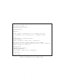
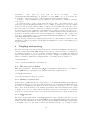
A minimal Sweave file is shown in Figure 1, which contains two code chunks embedded in a
simple LATEX document. Running
> rnwfile <- system.file("Sweave", "example-1.Rnw", package = "utils")
> Sweave(rnwfile)
Writing to file example-1.tex
Processing code chunks with options ...
1 : echo keep.source term verbatim (example-1.Rnw:13)
2 : keep.source term verbatim pdf (example-1.Rnw:23)
You can now run (pdf)latex on 'example-1.tex'
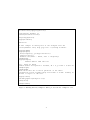
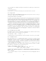
translates this into the LATEX document shown in Figures 2 and 3. The latter can also be created
directly from within R using
> tools::texi2pdf("example-1.tex")
The first difference between ‘example-1.Rnw’ and ‘example-1.tex’ is that the LATEX style
file ‘Sweave.sty’ is automatically loaded, which provides environments for typesetting R input
and output (the LATEX environments Sinput and Soutput). Otherwise, the documentation
chunks are copied without any modification from ‘example-1.Rnw’ to ‘example-1.tex’.
The real work of Sweave is done on the code chunks: The first code chunk has no name, hence
the default behavior of Sweave is used, which transfers both the R commands and their respective
output to the LATEX file, embedded in Sinput and Soutput environments, respectively.
The second code chunk shows one of the Sweave extension to the noweb syntax: Code chunk
names can be used to pass options to Sweave which control the final output.
• The chunk is marked as a figure chunk (fig=TRUE) such that Sweave creates (by default) a PDF file of the plot created by the commands in the chunk. Furthermore, a
\includegraphics{example-1-002} statement is inserted into the LATEX file (details on
the choice of file names for figures follow later in this manual).
• Option echo=FALSE indicates that the R input should not be included in the final document
(no Sinput environment).
3.2
Sweave options
Options control how code chunks and their output (text, figures) are transferred from the ‘.Rnw’
file to the ‘.tex’ file. All options have the form key=value, where value can be a number,
2
\ documentclass [ a4paper ]{ article }
\ title { Sweave Example 1}
\ author { Friedrich Leisch }
\ begin { document }
\ maketitle
In this example we embed parts of the examples from the
\ texttt { kruskal . test } help page into a \ LaTeX {} document :
< < > >=
data ( airquality , package =" datasets ")
library (" stats ")
kruskal . test ( Ozone ~ Month , data = airquality )
@
which shows that the location parameter of the Ozone
distribution varies significantly from month to month . Finally we
include a boxplot of the data :
\ begin { center }
<< fig = TRUE , echo = FALSE > >=
library (" graphics ")
boxplot ( Ozone ~ Month , data = airquality )
@
\ end { center }
\ end { document }
Figure 1: A minimal Sweave file: ‘example-1.Rnw’.
3
\ documentclass [ a4paper ]{ article }
\ title { Sweave Example 1}
\ author { Friedrich Leisch }
\ usepackage { Sweave }
\ begin { document }
\ maketitle
In this example we embed parts of the examples from the
\ texttt { kruskal . test } help page into a \ LaTeX {} document :
\ begin { Schunk }
\ begin { Sinput }
> data ( airquality , package =" datasets ")
> library (" stats ")
> kruskal . test ( Ozone ~ Month , data = airquality )
\ end { Sinput }
\ begin { Soutput }
Kruskal - Wallis rank sum test
data : Ozone by Month
Kruskal - Wallis chi - squared = 29.2666 , df = 4 , p - value = 6.901 e -06
\ end { Soutput }
\ end { Schunk }
which shows that the location parameter of the Ozone
distribution varies significantly from month to month . Finally we
include a boxplot of the data :
\ begin { center }
\ includegraphics { example -1 -002}
\ end { center }
\ end { document }
Figure 2: Running Sweave("example-1.Rnw") produces the file ‘example-1.tex’.
4
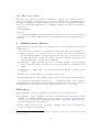
Sweave Example 1
Friedrich Leisch
July 10, 2014
In this example we embed parts of the examples from the kruskal.test
help page into a LATEX document:
> data(airquality, package="datasets")
> library("stats")
> kruskal.test(Ozone ~ Month, data = airquality)
Kruskal-Wallis rank sum test
data: Ozone by Month
Kruskal-Wallis chi-squared = 29.2666, df = 4, p-value = 6.901e-06
150
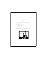
which shows that the location parameter of the Ozone distribution varies significantly from month to month. Finally we include a boxplot of the data:
100
●
●
●
●
●
0
50
●
5
6
7
8
9
1
Figure 3: The final document is created by running pdflatex on ‘example-1.tex’.
5
string or logical value. Several options can be specified at once (separated by commas), all
options must take a value (which must not contain a comma or equal sign). Logical options can
take the values TRUE, FALSE, T, F as well as lower-case and capitalized versions of the first two.
In the ‘.Rnw’ file options can be specified either
1. inside the angle brackets at the beginning of a code chunk, modifying the behaviour only
for this chunk, or
2. anywhere in a documentation chunk using the command
\SweaveOpts{opt1=value1, opt2=value2, ..., optN=valueN}
which modifies the defaults for the rest of the document, i.e., all code chunks after the
statement. Hence, an \SweaveOpts statement in the preamble of the document sets defaults for all code chunks.
Further, global options can be specified (as a comma-separated list of key=value items) in the
environment variable SWEAVE_OPTIONS, and via the --options= flag of R CMD Sweave.
Which options are supported depends on the driver in use. All drivers should at least support
the following options (all options appear together with their default value, if any):
split=FALSE: a logical value. If TRUE, then the output is distributed over several files, if
FALSE all output is written to a single file. Details depend on the driver.
label: a text label for the code chunk, which is used for file-name creation when split=TRUE. It
is also used in the comments added above the chunk when the file is processed by Rtangle
(provided the annotate option is true, as it is by default), and as part of the file names
for files generated by figure chunks.
Because labels can be part of file names, they should contain only alphanumeric characters
and #+-_. (Including . can cause confusion with file extensions.)
The first (and only the first) option in a code chunk name can be optionally without a name,
then it is taken to be a label. I.e., starting a code chunk with
<<hello, split=FALSE>>
is the same as
<<split=FALSE, label=hello>>
but
<<split=FALSE, hello>>
gives a syntax error. Having an unnamed first argument for labels is needed for noweb compatibility. If only \SweaveOpts is used for setting options, then Sweave files can be written to be
fully compatible with noweb (as only file names appear in code chunk names).
Note that split=TRUE should not be used in package vignettes.
The help pages for RweaveLatex and Rtangle list the options supported by the default
Sweave and Stangle drivers.
Now for the promised details on the file names corresponding to figures. These are of
the form prefix-label.ext. Here prefix can be set by the option prefix.string, otherwise is the basename of the output file (which unless specified otherwise is the basename of
the input file). label is the label of the code chunk if it has one, otherwise the number of
the code chunk in the range 001 to 999. ext is the appropriate extension for the type of
graphics, e.g. pdf, eps, . . . . So for the ‘example-1.Rnw’ file, the PDF version of the boxplot is ‘example-1-002.pdf’, since it is the second code chunk in the document. Note that
if prefix.string is used it can specify a directory as part of the prefix, so that for example
if \SweaveOpts{prefix.string=figures/fig}, the auto-generated figures will be placed in
sub-directory figures: the Sweave document should arrange to create this before use.
6
3.3
Using multiple input files
LATEX files can include others via \input{} commands. These can also be used in Sweave files,
but the included files will be included by LATEX and are not processed by Sweave. The equivalent
if you want the included files to be processed is the \SweaveInput{} command.
Included files should use the same Sweave syntax (see below) and encoding as the main file.
3.4
Using scalars in text
There is limited support for using the values of R objects in text chunks. Any occurrence of
\Sexpr{expr } is replaced by the string resulting from coercing the value of the expression expr
to a character vector; only the first element of this vector is used. E.g., 3 will be replaced by
the string ’3’ (without any quotes).
The expression is evaluated in the same environment as the code chunks, hence one can
access all objects defined in the code chunks which have appeared before the expression and
were evaluated. The expression may contain any valid R code, only braces ({ }) are not allowed.
(This is not really a limitation because more complicated computations can be easily done in a
hidden code chunk and the result then be used inside a \Sexpr.)
3.5
Code chunk reuse
Named code chunks can be reused in other code chunks following later in the document. Consider the simple example
<<a>>=
x <- 10
@
<<b>>=
x + y
@
<<c>>=
<<a>>
y <- 20
<<b>>
which is equivalent to defining the last code chunk as
<<c>>=
x <- 10
y <- 20
x + y
@
The chunk reference operator <<>> takes only the name of the chunk as its argument: no
additional Sweave options are allowed. It has to occur at the beginning of a line.
References to unknown chunk names are omitted, with a warning.
3.6
Syntax definition
So far we have only talked about Sweave files using noweb syntax (which is the default). However, Sweave allows the user to redefine the syntax marking documentation and code chunks,
using scalars in text or reuse code chunks.
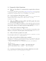
Figure 4 shows the example from Figure 1 using the SweaveSyntaxLatex definition. It can
be created using
7
\ documentclass [ a4paper ]{ article }
\ title { Sweave Example 1}
\ author { Friedrich Leisch }
\ begin { document }
\ maketitle
In this example we embed parts of the examples from the
\ texttt { kruskal . test } help page into a \ LaTeX {} document :
\ begin { Scode }{}
data ( airquality , package =" datasets ")
library (" stats ")
kruskal . test ( Ozone ~ Month , data = airquality )
\ end { Scode }
which shows that the location parameter of the Ozone
distribution varies significantly from month to month . Finally we
include a boxplot of the data :
\ begin { center }
\ begin { Scode }{ fig = TRUE , echo = FALSE }
library (" graphics ")
boxplot ( Ozone ~ Month , data = airquality )
\ end { Scode }
\ end { center }
\ end { document }
Figure 4: An Sweave file using LATEX syntax: ‘example-1.Stex’.
8
> SweaveSyntConv(rnwfile, SweaveSyntaxLatex)
Wrote file example-1.Stex
Code chunks are now enclosed in Scode environments, code chunk reuse is performed using
\Scoderef{chunkname}. All other operators are the same as in the noweb-style syntax.
Which syntax is used for a document is determined by the extension of the input file, files
with extension2 ‘.Rtex’ or ‘.Stex’ are assumed to follow the LATEX-style syntax. Alternatively
the syntax can be changed at any point within the document using the commands
\SweaveSyntax{SweaveSyntaxLatex}
or
\SweaveSyntax{SweaveSyntaxNoweb}
at the beginning of a line within a documentation chunk. Syntax definitions are simply lists
of regular expression for several Sweave commands: see the two default definitions mentioned
above for examples. (More detailed instructions will follow once the API has stabilized).
3.7
Encoding
LATEX documents are traditionally written entirely in ASCII, using LATEX escapes such as \'e
for accented characters. This can be inconvenient when writing a non-English document, and
an alternative input encoding can be selected by using a statement such as
\usepackage[latin1]{inputenc}
in the document’s preamble, to tell LATEX to translate the input to its own escapes. There is a
wide range of input encodings which are supported, at least partially, and the more recent LATEX
package inputenx supports more. Other encodings commonly encountered in Sweave documents
are latin9, utf8 and ansinew (the CP1252 codepage on Windows). Greater coverage3 of UTF8 can be obtained by
\usepackage[utf8]{inputenx} \input{ix-utf8enc.dfu}
As from R 3.1.0, the UTF-8 encoding is handled preferentially to other encodings. Whereas
Sweave will convert R code to the local encoding in general, it leaves UTF-8 code in that
encoding, and outputs in that encoding as well. Besides the declaration scheme above, a UTF-8
encoding may be obtained by the LATEX comment
%\SweaveUTF8
The previous paragraphs covered the documentation sections, but what of the code sections
where LATEX escapes cannot be used? The first piece of advice is to use only ASCII code sections
as anything else will reduce the portability of your document. But R code can be included if in
the input encoding declared in the preamble.
The next complication is inclusions: the final vignette may well include R output, LATEX or
other Sweave files via \input{} and \SweaveInput{} lines, a bibliography and figures. It is the
user’s responsibility that the text inclusions are covered by the declared input encoding. LATEX
allows the input encoding to be changed by
\inputencoding{something}
2 or
the lowercase versions, for convenience on case-insensitive file systems.
Eastern European, Greek and Hebrew letters.
3 including
9
statements:
these may not work well in Sweave processing.
Since
\usepackage[latin1]{inputenc} is typically not legal LATEX code in an included file,
it is easiest to declare the encoding to Sweave using the %\SweaveUTF8 comment.
It is all too easy for BiBTeX to pick up UTF-8-encoded references for a Latin-1 document,
or vice versa.
R output is again to a large extent under the user’s control. If a Latin-1 Sweave document is processed by R running a Latin-1 locale or a UTF-8 document is processed in a UTF-8
locale, the only problems which are likely to arise are from handling data in another encoding, but it may be necessary to declare the document’s encoding to cover the R output which
is generated even if the document is itself ASCII. One common problem is the quotes produced by \sQuote() and \dQuote(): these will be in UTF-8 when R is run in a UTF-8 locale,
and will be in CP1252 when Sweave is run from Rgui.exe on Windows. Two possible solutions are to suppress fancy quotes by options(useFancyQuotes=FALSE) or to force UTF-8 by
options(useFancyQuotes="UTF-8").
The encoding of figures is not usually an issue as they are either bitmaps or include encoding
information: it may be necessary to use the pdf.encoding Sweave option to set the pdf() device
up appropriately.
4
Tangling and weaving
The user front-ends of the Sweave system are the two R functions Stangle() and Sweave(),
both are contained in package utils. Stangle can be used to extract only the code chunks from
an ‘.Rnw’ file and write to one or several files. Sweave() runs the code chunks through R and
replaces them with the respective input and/or output. Stangle is actually just a wrapper
function for Sweave, which uses a tangling instead of a weaving driver by default. See
> help("Sweave")
for more details and arguments of the functions.
4.1
The RweaveLatex driver
This driver transforms ‘.Rnw’ files with LATEX documentation chunks and R code chunks to
proper LATEX files (for typesetting both with standard latex or pdflatex), see
> help("RweaveLatex")
for details, including the supported options.
4.1.1
Writing to separate files
If split is set to TRUE, then all text corresponding to code chunks (the Sinput and Soutput environments) is written to separate files. The file names are of form ‘prefix.string-label.tex’,
if several code chunks have the same label, their outputs are concatenated. If a code chunk
has no label, then the number of the chunk is used instead. The same naming scheme applies
to figures. You do need to ensure that the file names generated are valid and not so long that
there are not regarded as the same by your OS (some file systems only recognize 13 characters).
4.1.2
LATEX style file
The driver automatically inserts a \usepackage{Sweave.sty} command as last line before the
\begin{document} statement of the final LATEX file if no \usepackage{Sweave} is found in the
Sweave source file. This style file defines the environments Sinput and Soutput for typesetting
code chunks. If you do not want to include the standard style file, e.g., because you have
10
your own definitions for Sinput and Soutput environments in a different place, simply insert a
comment like
% \usepackage{Sweave}
in the preamble of your latex file, this will prevent automatic insertion of the line.
4.1.3
Figure sizes
‘Sweave.sty’ sets the default LATEX figure width (which is independent of the size of the generated EPS or PDF files). The current default is
\setkeys{Gin}{width=0.8\textwidth}
if you want to use another width for the figures that are automatically generated and included
by Sweave, simply add a line similar to the one above after \begin{document}. If you want no
default width for figures insert a \usepackage[nogin]{Sweave} in the header of your file. Note
that a new graphics device is opened for each figure chunk (one with option fig=TRUE), hence
all graphical parameters of the par() command must be set in each single figure chunk and are
forgotten after the respective chunk (because the device is closed when leaving the chunk).
Attention: One thing that gets easily confused are the width/height parameters of the R
graphics devices and the corresponding arguments to the LATEX \includegraphics command.
The Sweave options width and height are passed to the R graphics devices, and hence affect
the default size of the produced EPS and PDF files. They do not affect the size of figures in the
document, by default they will always be 80% of the current text width. Use \setkeys{Gin}
to modify figure sizes or use explicit \includegraphics commands in combination with the
Sweave option include=FALSE.
4.1.4
Prompts and text width
By default the driver gets the prompts used for input lines and continuation lines from R’s
options() settings. To set new prompts use something like
options(prompt = "MyR> ", continue = "...")
see help(options) for details. Similarly the output text width is controlled by option "width".
4.1.5
Graphics devices
The default graphics device for fig=TRUE chunks is pdf(): the standard options pdf, eps, png
and jpg allow one or more of these to be selected for a particular chunk or (via \SweaveOpts)
for the whole document. It can be convenient to select PNG for a particular figure chunk by
something like <<figN, fig=TRUE, pdf=FALSE, png=TRUE>>: pdflatex should automatically
include the PNG file for that chunk.
You can define your own graphics devices and select one of them by the option
grdevice=my.Swd where the device function (here my.Swd) is defined in a hidden code chunk.
For example, we could make use of the cairo_pdf device by
my.Swd <- function(name, width, height, ...)
grDevices::cairo_pdf(filename = paste(name, "pdf", sep = "."),
width = width, height = height)
Specialized custom graphics devices may need a customized way to shut them down in place of
graphics.off(): this can be supplied via a companion function my.Swd.off, which is called
with no arguments.
For a complete example see the file ‘src/library/utils/tests/customgraphics.Rnw’ in
the R sources.
11
4.2
The Rtangle driver
This driver can be used to extract R code chunks from a ‘.Rnw’ file. Code chunks can either be
written to one large file or separate files (one for each code chunk). The options split, prefix,
and prefix.string have the same defaults and interpretation as for the RweaveLatex driver.
Use the standard noweb command line tool notangle if chunks other than R code should be
extracted. See
> help("Rtangle")
for details.
Note that split=TRUE rarely makes much sense, as the files produced are often interdependent and need to be run in a particular order, an order which is often not the alphabetical order
of the files.
5
Adding Sweave Drivers
Adding drivers is relatively simple by modelling them on4 the existing RweaveLatex and
Rtangle drivers.
An Sweave driver is a function of no arguments which should return a list of five functions:
setup(file, syntax, ...): Set up the driver, e.g. open the output file. Its return value is
an object which is passed to the next three functions, and can be updated by the next
two. The value should be a list, and contain a component options, a named list of the
default settings for the options needed by runcode.
runcode(object, chunk, options): Process a code chunk. Returns a possibly updated
object. Argument chunk is a character vector, and options is a options list for this
chunk.
writedoc(object, chunk): Write out a documentation chunk. Returns a possibly updated
object.
finish(object, error): Finish up, or clean up if error is true.
checkopts(options): Converts/validates options given as a named list of character strings.
Note that the setup function should have a ... argument. It will be passed additional
arguments from a Sweave() call, but in future Sweave may itself set options and pass them on
the setup function: one such may be the encoding used for the text to be processed.
References
Knuth DE (1984). “Literate Programming.” The Computer Journal, 27(2), 97–111.
Leisch F (2002). “Sweave: Dynamic Generation of Statistical Reports Using Literate Data
Analysis.” In W Härdle, B Rönz (eds.), Compstat 2002 — Proceedings in Computational
Statistics, pp. 575–580. Physica Verlag, Heidelberg. ISBN 3-7908-1517-9, URL http://www.
stat.uni-muenchen.de/~leisch/Sweave.
Ramsey N (1998). Noweb man page. University of Virginia, USA. Version 2.9a, URL http:
//www.cs.virginia.edu/~nr/noweb.
4 but if you copy, do be careful not to infringe R-core’s copyright: the copyright notices in the R sources must
also be copied.
12
A
A.1
Frequently Asked Questions
How can I get Emacs to automatically recognize files in Sweave
format?
Recent versions of ESS (Emacs speaks statistics, http://ess.R-project.org) automatically
recognize files with extension ‘.Rnw’ as Sweave files and turn on the correct modes. Please follow
the instructions on the ESS homepage on how to install ESS on your computer.
A.2
Can I run Sweave directly from a shell?
E.g., for writing makefiles it can be useful to run Sweave directly from a shell rather than
manually starting R and then running Sweave. This can easily be done using
R CMD Sweave file.Rnw
A.3
Why does LATEX not find my EPS and PDF graphic files when
the file name contains a dot?
Sweave uses the standard LATEX package graphicx to handle graphic files, which automatically
chooses the type of file, provided the basename given in the \includegraphics{} statement
has no extension. Hence, you may run into trouble with graphics handling if the basename of
your Sweave file contains dots: ‘foo.Rnw’ is OK, while ‘foo.bar.Rnw’ is not.
A.4
Empty figure chunks give LATEX errors.
When a code chunk with fig=TRUE does not call any plotting functions, invalid PDF (or EPS)
files may be created. Sweave cannot know if the code in a figure chunk actually plotted something or not, so it will try to include the graphics, which is bound to fail.
A.5
Why do R lattice graphics not work?
In recent versions of Sweave they do if they would when run at the command line: some calls
(e.g. those inside loops) need to be explicitly print()-ed.
A.6
How can I get Black & White lattice graphics?
What is the most elegant way to specify that strip panels are to have transparent backgrounds
and graphs are to be in black and white when lattice is being used with Sweave? I would prefer
a global option that stays in effect for multiple plots.
Answer by Deepayan Sarkar: I’d do something like this as part of the initialization:
<<...>>
library(lattice)
ltheme <- canonical.theme(color = FALSE)
## in-built B&W theme
ltheme$strip.background$col <- "transparent" ## change strip bg
lattice.options(default.theme = ltheme)
## set as default
@
A.7
Creating several figures from one figure chunk does not work
Consider that you want to create several graphs in a loop similar to
13
<<fig=TRUE>>
for (i in 1:4) plot(rnorm(100)+i)
@
This will currently not work, because Sweave allows only one graph per figure chunk. The
simple reason is that Sweave opens a pdf device before executing the code and closes it afterwards. If you need to plot in a loop, you have to program it along the lines of
<<results=tex,echo=FALSE>>=
for(i in 1:4){
fname <- paste("myfile", i, ".pdf", sep = "")
pdf(file = fname, width = 6, height = 6)
plot(rnorm(100)+i)
dev.off()
cat("\\includegraphics{", fname, "}\n\n", sep = "")
}
@
A.8
How can I set default par() settings for figure chunks?
Because Sweave opens a new device for each graphics file in each figure chunk, using par() has
only an effect if it is used inside a figure chunk. If you want to use the same settings for a series
of figures, it is easier to use a hook function than repeating the same par() statement in each
figure chunk.
The effect of
options(SweaveHooks = list(fig = function() par(bg = "red", fg = "blue")))
should be easy to spot.
A.9
How can I change the formatting of R input and output chunks?
Sweave uses the fancyvrb package for formatting all R code and text output. fancyvrb is a very
powerful and flexible package that allows fine control for layouting text in verbatim environments. If you want to change the default layout, simply read the fancyvrb documentation and
modify the definitions of the Sinput and Soutput environments in ‘Sweave.sty’, respectively.
A.10
How can I change the line length of R input and output?
Sweave respects the usual way of specifying the desired line length in R, namely
options(width). E.g., after options(width = 40) lines will be formatted to have at most
40 characters (if possible).
A.11
Can I use Sweave for Word files?
Not directly, but package SWord provides similar functionality for Microsoft Word on Windows
platforms.
A.12
Can I use Sweave for OpenOffice files?
Yes, package odfWeave provides functions for using Sweave in combination with OpenOffice
Writer rather than LATEX.
14
A.13
Can I use Sweave for HTML files?
Yes, package R2HTML provides a driver for using Sweave in combination with HTML rather
than LATEX.
A.14
After loading package R2HTML Sweave doesn’t work properly!
Package R2HTML registers an Sweave driver for HTML files using the same file extensions
as the default noweb syntax, and after that its syntax is on the search list before the default
syntax. Using
options(SweaveSyntax = "SweaveSyntaxNoweb")
or calling Sweave like
Sweave(..., syntax = "SweaveSyntaxNoweb")
ensures the default syntax even after loading package R2HTML.
15