Download as a PDF

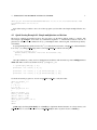
GF-Complete: A Comprehensive Open Source Library for Galois
Field Arithmetic
Version 0.1 - February, 2013
James S. Plank∗
Ethan L. Miller
William B. Houston
Technical Report UT-CS-13-703
Department of Electrical Engineering and Computer Science
University of Tennessee, Knoxville, TN 37996
http://www.cs.utk.edu/˜plank/plank/papers/CS-13-703.html
This is a user’s manual for GF-Complete, version 0.1. This is a pre-release, mostly because the documentation is
incomplete. We anticipate that version 1.0 will follow around May or June of 2013, where the code will be cleaner,
and we may have a few more things implemented, but more importantly, this user’s manual will be complete with
more description, examples and hand-holding. Additionally, by that time, we will have a journal manuscript written
that goes over all of the implementation techniques in detail.
The important part of this release is that it is the first public unveiling of performing region multiplication using the
Intel SIMD instructions, which makes it blazingly fast. This is described in our Usenix FAST paper in 2013 [PGM13].
We will not change the interface when we post revision 1.0.
If You Use This Library or Document
Please send me an email to let me know how it goes. Or send me an email just to let me know you are using the
library. One of the ways in which we are evaluated both internally and externally is by the impact of our work, and if
you have found this library and/or this document useful, we would like to be able to document it. Please send mail to
[email protected]. Please send bug reports to that address as well.
The library itself is protected by the New BSD License. It is free to use and modify within the bounds of this
license. None of the techniques implemented in this library have been patented.
Finding the Code
Please see http://www.cs.utk.edu/˜plank/plank/papers/CS-13-703.html to get the tar file for
this code.
∗ [email protected] (Tennessee), [email protected] (UC Santa Cruz). This material is based upon work supported by the National
Science Foundation under grants CNS-0917396,, IIP-0934401 and CSR-1016636. Special thanks to Kevin Greenan who wrote significant parts of
the library.
1
CONTENTS
2
Contents
1
Introduction
1.1 Limitations to Revision 0.1 . . . . . . . . . . . . . . . . . . . . . . . . . . . . . . . . . . . . . . . .
3
4
2
Files in the Library
4
3
Compilation, especially with regard to the SSE instructions
6
4
Some Tools and Examples to Get You Started
4.1 Three Simple Command Line Tools: gf mult, gf div and gf add
4.2 Quick Starting Example #1: Simple multiplication and division .
4.3 Quick Starting Example #2: Multiplying a region by a constant .
4.4 Quick Starting Example #3: Using w = 64 . . . . . . . . . . .
4.5 Quick Starting Example #4: Using w = 128 . . . . . . . . . . .
.
.
.
.
.
7
7
8
9
9
10
5
Alignment and Information on the Defaults
5.1 Important Information on Alignment when Multiplying Regions . . . . . . . . . . . . . . . . . . . .
5.2 The Defaults . . . . . . . . . . . . . . . . . . . . . . . . . . . . . . . . . . . . . . . . . . . . . . . .
10
10
11
6
Changing the Defaults
6.1 Changing the Defaults with create gf from argv()
6.1.1 Alternate specifications for w = 4 . . . . .
6.1.2 Alternate specifications for w = 8 . . . . .
6.1.3 Alternate specifications for w = 16 . . . .
6.1.4 Alternate specifications for w = 32 . . . .
6.1.5 Alternate specifications for w = 64 . . . .
6.1.6 Alternate specifications for w = 128 . . . .
6.2 Calling gf init hard() . . . . . . . . . . . . . . . .
11
12
14
14
14
15
17
18
19
7
Thread Safety
.
.
.
.
.
.
.
.
.
.
.
.
.
.
.
.
.
.
.
.
.
.
.
.
.
.
.
.
.
.
.
.
.
.
.
.
.
.
.
.
.
.
.
.
.
.
.
.
.
.
.
.
.
.
.
.
.
.
.
.
.
.
.
.
.
.
.
.
.
.
.
.
.
.
.
.
.
.
.
.
.
.
.
.
.
.
.
.
.
.
.
.
.
.
.
.
.
.
.
.
.
.
.
.
.
.
.
.
.
.
.
.
.
.
.
.
.
.
.
.
.
.
.
.
.
.
.
.
.
.
.
.
.
.
.
.
.
.
.
.
.
.
.
.
.
.
.
.
.
.
.
.
.
.
.
.
.
.
.
.
.
.
.
.
.
.
.
.
.
.
.
.
.
.
.
.
.
.
.
.
.
.
.
.
.
.
.
.
.
.
.
.
.
.
.
.
.
.
.
.
.
.
.
.
.
.
.
.
.
.
.
.
.
.
.
.
.
.
.
.
.
.
.
.
.
.
.
.
.
.
.
.
.
.
.
.
.
.
.
.
.
.
.
.
.
.
.
.
.
.
.
.
.
.
.
.
.
.
.
.
.
.
.
.
.
.
.
.
.
.
.
.
.
.
.
.
.
.
.
.
.
.
.
.
.
.
.
.
.
.
.
.
.
.
.
.
.
.
.
.
.
.
.
.
.
.
.
.
.
.
.
20
1
1
INTRODUCTION
3
Introduction
Galois Field arithmetic forms the backbone of erasure-coded storage systems, most famously the Reed-Solomon
erasure code. A Galois Field is defined over w-bit words and is termed GF (2w ). As such, the elements of a Galois
Field are the integers 0, 1, . . ., 2w − 1. Galois Field arithmetic defines addition and multiplication over these closed
sets of integers in such a way that they work as you would hope they would work. Specifically, every number has a
unique multiplicative inverse. Moreover, there is a value, typically the value 2, which has the property that you can
enumerate all of the non-zero elements of the field by taking that value to successively higher powers.
Addition in a Galois Field is equal to the bitwise exclusive-or operation. That’s nice and convenient. Multiplication
is a little more complex, and there are many, many ways to implement it. Here are a few references that describe various
ways to implement multiplication: [GMS08, LD00, LBOX12, Pla97]. The intent of this library is to implement all of
the techniques. That way, their performance may be compared, and their tradeoffs may be analyzed.
When used for erasure codes, there are typically five important operations:
1. Adding two numbers in GF (2w ). That’s bitwise exclusive-or.
2. Multiplying two numbers in GF (2w ). Erasure codes are usually based on matrices in GF (2w ), and constructing these matrices requires addition and multiplication.
3. Dividing two numbers in GF (2w ). Sometimes you need to divide to construct matrices (for example, Cauchy
Reed-Solomon codes [BKK+ 95, Rab89]). More often, though, you use division to invert matrices for decoding.
Sometimes it is easier to find a number’s inverse than it is to divide. In that case, you can divide by multiplying
by an inverse.
4. Adding two regions of numbers in GF (2w ). See below.
5. Mutiplying a region of numbers in GF (2w ) by a constant in GF (2w ). Erasure coding typically boils down
to performing dot products in GF (2w ). For example, you may define a coding disk using the equation:
c0 = d0 + ad1 + a2 d2 + a3 d3 .
That looks like three multiplications and three additions However, the way that’s implemented in a disk system
looks as in Figure 1. Large regions of disks are partitioned into w-bit words in GF (2w ). In the example,
let us suppose that w = 8. Then the regions pictured are 1 KB from each disk. The words on disk Di are
labeled di,0 , di,1 , . . . , di,1023 , and the equation above is replicated 1024 times. For 0 ≤ j < 1024:
c0,j = d0,j + ad1,j + a2 d2,j + a3 d3,j .
While it’s possible to implement adding two regions and multiplying a region by a constant by using the single
operations, it is often much more efficient to aggregate. For example, most computer architectures support
bitwise exclusive-or of 64 and 128 bit words. Thus, it makes much more sense to add regions of numbers in
64 or 128 bit chunks rather than as words in GF (2w ). Multiplying a region by a constant can leverage similar
optimizations.
GF-Complete supports multiplication and division of single values for all values of w ≤ 32, plus w = 64 and w =
128. It also supports adding two regions of memory (for any value of w, since addition equals XOR), and multiplying
a region by a constant in GF (24 ), GF (28 ), GF (216 ), GF (232 ), GF (264 ) and GF (2128 ). These values are chosen
because words in GF (2w ) fit into machine words with these values of w. Other values of w don’t lend themselves to
efficient multiplication of regions by constants.
2
FILES IN THE LIBRARY
4
Figure 1: An example of adding two regions of numbers, and multiplying a region of numbers by a constant
in GF (2w ). In this example, if w = 8, then each disk is holding a 1KB region, and the same coding equation —
c0,j = d0,j + ad1,j + a2 d2,j + a3 d3,j is applied 1024 times. It is often much more efficient to implement this by three
region-constant multiplications and three region-region additions.
1.1
Limitations to Revision 0.1
The code in revision 0.1 does a lot more than we have documented. The complete documentation will be released as
revision 1.0. We document the following parts of the library here.
1. Example programs to demonstrate use of the library. These help you play with Galois Field arithmetic,
and they help you get started with the library by using the default techniques for each value of w. For w =
4 and w = 8, these implementations are the fastest that we have. For larger values of w, there are faster
implementations, but we don’t include them in the defaults because they either employ an alternate mapping of
numbers to memory, or they use quite a lot of memory for tables.
2. Explanation of Alignment and Defaults. When you multiply a region of bytes by a constant, there are some
constraints on how your pointers are aligned. We go over this is detail. We also explain which default values are
not the fastest.
3. The unit tester and the timer. These are two important programs. The first checks implementations for
correctness. The second performs timings. If you are going to stray from the defaults, we urge you to run both
the unit tester and the timer to make sure that there are no problems on your processor, and to see how fast it’s
going.
4. How to do better than the defaults for w ≥ 16. This is where we explain how to change the defaults to get
faster behavior for the larger values of w.
2
Files in the Library
The following files compose GF-Complete. First, the header files:
2
FILES IN THE LIBRARY
5
• gf complete.h: This is the header file that applications should include. It defines the gf t type, which holds all
of the data that you need to perform the various operations in GF (2w ). It also defines all of the arithmetic operations. For an application to use this library, you should compile the library gf complete.a and then applications
include gf complete.h and compile with the library.
• gf method.h: This defines a few “helper” procedures to let you set the implementation techniques using the
Unix command line.
• gf general.h: This file has helper routines for doing basic Galois Field operations with any legal value of w.
The problem is that w ≤ 32, w = 64 and w = 128 all have different data types, which is a pain. The procedures
in this file try to alleviate that pain. They are used in gf unit and gf time. I’m guessing that most applications
won’t use them, as most applications use w ≤ 32.
• gf rand.h: I’ve learned that srand48() and its kin are not supported in all C installations. Therefore, this file
defines some random number generators to help test the programs. The random number generator is the “Mother
of All” random number generator [Mar94] which we’ve selected because it has no patent issues. gf unit and
gf time use these random number generators.
• gf int.h: This is a header file that defines common operations that the various source files use. This is not
intended for applications.
The following C files compose gf complete.a. You shouldn’t have to mess with these files, but we include them in
case you have to:
• gf.c: This implements all of the procedures in both gf complete.h and gf int.h.
• gf w4.c: Procedures specific to w = 4.
• gf w8.c: Procedures specific to w = 8.
• gf w16.c: Procedures specific to w = 16.
• gf w32.c: Procedures specific to w = 32.
• gf w64.c: Procedures specific to w = 64.
• gf w128.c: Procedures specific to w = 128.
• gf wgen.c: Procedures specific to other values of w between 1 and 31.
• gf general.c: Procedures that let you manipulate general values, regardless of whether w ≤ 32, w = 64
or w = 128.
• gf method.c: Procedures to help you switch between the various implementation techniques.
• gf rand.c: The “Mother of all” random number generator.
Finally, the following C files are example applications that use the library:
• gf mult.c, gf div.c and gf add: Command line tools explained below.
• gf example x.c: Example programs to help you use the library quickly.
3
COMPILATION, ESPECIALLY WITH REGARD TO THE SSE INSTRUCTIONS
6
• gf unit.c: A unit tester to verify that all of the procedures work for given values of w and implementation
options.
• gf time.c: A program that times the procedures for given values of w and implementation options.
• gf poly.c: A program to help find primitive polynomials in composite fields (see [GMS08] for more explanation
on this).
3
Compilation, especially with regard to the SSE instructions
This is not a complex library, so simply using make should be sufficient. The makefile (in GNUmakefile assumes that
the Intel SSE4 instructions are supported, and thus compiles with the flags: -msse4 -DINTEL SSE4. If you wish to
compile the library with out the SSE flags, then remove those flags from the GNUmakefile.
We’ve included a program called whats my sse.c. When you compile and run it, it will tell you what SSE instructions it supports. For example, this is on my MacBook Pro (Intel Core i5), which has support through SSE4:
UNIX> gcc whats_my_sse.c
UNIX> a.out
1 - Instruction set is supported by CPU
0 - Instruction set not supported
-------------------------------MMX:
1
SSE:
1
SSE2:
1
SSE3:
1
SSE4.1: 1
SSE4.2: 1
SSEAVX: 0
UNIX>
On the flip side, here is Linux box, which only has support through SSE3. With this processor, you must compile
without the -msse4 and -DINTEL SSE4 flags.
UNIX> grep model /proc/cpuinfo
model : 4
model name : Intel(R) Pentium(R) 4 CPU 3.40GHz
model : 4
model name : Intel(R) Pentium(R) 4 CPU 3.40GHz
UNIX> gcc whats_my_sse.c
UNIX> a.out
1 - Instruction set is supported by CPU
0 - Instruction set not supported
-------------------------------MMX:
1
SSE:
1
SSE2:
1
SSE3:
1
SSE4.1: 0
SSE4.2: 0
4
SOME TOOLS AND EXAMPLES TO GET YOU STARTED
SSEAVX:
UNIX>
7
0
Our recommendation is to not compile the library with the SSE flags unless you have SSE4.2. Thanks to Jens
Gregor for giving us whats my sse.c.
After you make, the library will be in gf complete.a. To use the library, include gf complete.h in your C programs
and create your executable with gf complete.a.
4
4.1
Some Tools and Examples to Get You Started
Three Simple Command Line Tools: gf mult, gf div and gf add
Before delving into the library, it may be helpful to explore Galois Field arithmetic with the command line tools:
gf mult, gf div and gf add. These perform multiplication, division and addition on elements in GF (2w ). The syntax
is:
• gf mult a b w - Multiplies a and b in GF (2w ).
• gf div a b w - Divides a by b in GF (2w ).
• gf add a b w - Adds a and b in GF (2w ).
You may use any value of w from 1 to 32, plus 64 and 128. By default, the values are read and printed in decimal;
however, if you append an ’h’ to w, then a, b and the result will be printed in hexadecimal. For w ∈ {64, 128}, the ’h’
is mandatory, and all values will be printed in hexadecimal.
Try them out on some examples like the ones below. You of course don’t need to know that, for example, 5 ∗ 4 = 7
in GF (24 ); however, once you know that, you know that 57 = 4 and 74 = 5. You should be able to verify the gf add
statements below in your head. As for the other gf mult’s, you can simply verify that division and multiplication work
with each other as you hope they would.
UNIX> gf_mult 5 4 4
7
UNIX> gf_div 7 5 4
4
UNIX> gf_div 7 4 4
5
UNIX> gf_mult 8000 2 16h
100b
UNIX> gf_add f0f0f0f0f0f0f0f0 1313131313131313 64h
e3e3e3e3e3e3e3e3
UNIX> gf_mult f0f0f0f0f0f0f0f0 1313131313131313 64h
8da08da08da08da0
UNIX> gf_div 8da08da08da08da0 1313131313131313 64h
f0f0f0f0f0f0f0f0
UNIX> gf_add f0f0f0f0f0f0f0f01313131313131313 1313131313131313f0f0f0f0f0f0f0f0 128h
e3e3e3e3e3e3e3e3e3e3e3e3e3e3e3e3
UNIX> gf_mult f0f0f0f0f0f0f0f01313131313131313 1313131313131313f0f0f0f0f0f0f0f0 128h
786278627862784982d782d782d7816e
4
SOME TOOLS AND EXAMPLES TO GET YOU STARTED
8
UNIX> gf_div 786278627862784982d782d782d7816e f0f0f0f0f0f0f0f01313131313131313 128h
1313131313131313f0f0f0f0f0f0f0f0
UNIX>
Don’t bother trying to read the source code of these programs yet. Start with some simpler examples like the ones
below.
4.2
Quick Starting Example #1: Simple multiplication and division
The next two examples are intended for those who just want to use the library without getting too complex. The
first example is gf example 1, and it takes one command line argument – w, which must be between 1 and 32. It
generates two random non-zero numbers in GF (2w ), and multiplies them. After doing that, it divides the product by
each number.
To perform multiplication and division in GF (2w ), you must declare an instance of the gf t type, and then initialize
it for GF (2w ) by calling gf init easy(). This is done in gf example 1.c with the following lines:
if (!gf_init_easy(&gf, w)) {
fprintf(stderr, "Couldn’t initialize GF structure.\n");
exit(0);
}
Once gf is initialized, you may use it for multiplication and division with the function pointers multiply.w32 and
divide.w32. These work for any element of GF (2w ) so long as w ≤ 32.
c = gf.multiply.w32(&gf, a, b);
printf("%u * %u = %u\n", a, b, c);
printf("%u / %u = %u\n", c, a, gf.divide.w32(&gf, c, a));
printf("%u / %u = %u\n", c, b, gf.divide.w32(&gf, c, b));
Go ahead and test this program out. You can use gf mult and gf div to verify the results:
UNIX> gf_example_1 4
12 * 4 = 5
5 / 12 = 4
5 / 4 = 12
UNIX> gf_mult 12 4 4
5
UNIX> gf_example_1 16
14411 * 60911 = 44568
44568 / 14411 = 60911
44568 / 60911 = 14411
UNIX> gf_mult 14411 60911 16
44568
UNIX>
gf init easy() (and later gf init hard()) do call malloc() to implement internal structures. To release memory, call
gf free(). Please see section 6.2 to see how to call gf init hard() in such a way that it doesn’t call malloc().
4
SOME TOOLS AND EXAMPLES TO GET YOU STARTED
4.3
9
Quick Starting Example #2: Multiplying a region by a constant
The program gf example 2 expands on gf example 1. If w is equal to 4, 8, 16 or 32, it performs a region multiply
operation. It allocates two sixteen byte regions, r1 and r2, and then multiples r1 by a and puts the result in r2 using
the multiply region.w32 function pointer:
gf.multiply_region.w32(&gf, r1, r2, a, 16, 0);
That last argument specifies whether to simply place the product into r2 or to XOR it with the contents that are
already in r2. Zero means to place the product there. When we run it, it prints the results of the multiply region.w32
in hexadecimal. Again, you can verify it using gf mult:
UNIX> gf_example_2 4
12 * 2 = 11
11 / 12 = 2
11 / 2 = 12
multiply_region by 0xc (12)
R1 (the source):
0 2 d 9 d 6 8 a 8 d b 3 5 c 1 8 8 e b 0 6 1 5 a 2 c 4 b 3 9 3 6
R2 (the product): 0 b 3 6 3 e a 1 a 3 d 7 9 f c a a 4 d 0 e c 9 1 b f 5 d 7 6 7 e
UNIX> gf_example_2 16
49598 * 35999 = 19867
19867 / 49598 = 35999
19867 / 35999 = 49598
multiply_region by 0xc1be (49598)
R1 (the source):
R2 (the product):
UNIX> gf_mult c1be
4d9b
UNIX> gf_mult c1be
992d
UNIX>
4.4
8c9f b30e 5bf3 7cbb 16a9 105d 9368 4bbe
4d9b 992d 02f2 c95c 228e ec82 324e 35e4
8c9f 16h
b30e 16h
Quick Starting Example #3: Using w = 64
The program in gf example 3.c is identical to the previous program, except it uses GF (264 ). Now a, b and c are
uint64 t’s, and you have to use the function pointers that have w64 extensions so that the larger types may be employed.
UNIX> gf_example_3
a9af3adef0d23242 * 61fd8433b25fe7cd = bf5acdde4c41ee0c
bf5acdde4c41ee0c / a9af3adef0d23242 = 61fd8433b25fe7cd
bf5acdde4c41ee0c / 61fd8433b25fe7cd = a9af3adef0d23242
multiply_region by a9af3adef0d23242
5
ALIGNMENT AND INFORMATION ON THE DEFAULTS
10
R1 (the source):
61fd8433b25fe7cd 272d5d4b19ca44b7 3870bf7e63c3451a 08992149b3e2f8b7
R2 (the product): bf5acdde4c41ee0c ad2d786c6e4d66b7 43a7d857503fd261 d3d29c7be46b1f7c
UNIX> gf_mult a9af3adef0d23242 61fd8433b25fe7cd 64h
bf5acdde4c41ee0c
UNIX>
4.5
Quick Starting Example #4: Using w = 128
Finally, the program in gf example 4.c uses GF (2128 ). Since there is not universal support for uint128 t, the library
represents 128-bit numbers as arrays of two uint64 t’s. The function pointers for multiplication, division and region
multiplication now accept the return values as arguments:
gf.multiply.w128(&gf, a, b, c);
Again, we can use gf mult and gf div to verify the results:
UNIX> gf_example_4
e252d9c145c0bf29b85b21a1ae2921fa * b23044e7f45daf4d70695fb7bf249432 =
7883669ef3001d7fabf83784d52eb414
multiply_region by e252d9c145c0bf29b85b21a1ae2921fa
R1 (the source):
f4f56f08fa92494c5faa57ddcd874149 b4c06a61adbbec2f4b0ffc68e43008cb
R2 (the product): b1e34d34b031660676965b868b892043 382f12719ffe3978385f5d97540a13a1
UNIX> gf_mult e252d9c145c0bf29b85b21a1ae2921fa f4f56f08fa92494c5faa57ddcd874149 128h
b1e34d34b031660676965b868b892043
UNIX> gf_div 382f12719ffe3978385f5d97540a13a1 b4c06a61adbbec2f4b0ffc68e43008cb 128h
e252d9c145c0bf29b85b21a1ae2921fa
UNIX>
5
Alignment and Information on the Defaults
5.1
Important Information on Alignment when Multiplying Regions
In order to make multiplication of regions fast, we often employ 64 and 128 bit instructions (see [PGM13] for how we
use Intel’s SIMD instructions to have region multiplication scream along at cache line speeds). For that reason, we are
stringent about alignment of the source and destination regions:
When you perform multiply region.wxx(gf, source, dest, value, size, add), there are three requirements:
1. source and dest must be aligned for w-bit words. For w = 4 and w = 8, there is no restriction; however for
w = 16, the pointers must be multiples of 2, for w = 32, they must be multiples of 4 and for w ∈ {64, 128},
they must be multiples of 8.
2. size must be a multiple of w8 . With w = 4 and w = 8, there is no restriction; however the other sizes must be
multiples of w8 because you have to be multiplying whole elements of GF (2w ).
6
CHANGING THE DEFAULTS
11
3. (source mod 16) and (dest mod 16) must equal each other. Typically, this is not a worry, because most of the
time you will use malloc() to allocate memory, and the pointers that it returns will have the proper alignment.
However, in order to leverage the SIMD instructions, the two pointers must have the same alignment with
respect to 128-bit words. When we write up the big version of this library, we’ll tell you how you can relax this
requirement, but until then, you need to pay attention to alignment.
5.2
The Defaults
The default Galois Field implementations have been designed for a combination of speed, memory and convenience.
Here are some descriptions:
• For w = 4, the multiply.w32() and divide.w32() implementations use 16×16 tables. The multiply region.w32()
operation uses table lookup with the SIMD instructions exactly as outlined in [PGM13]. This will be fast. If the
processor does not support SSE4, then simple table lookup is employed, which is much slower.
• For w = 8, the implementations are the same as w = 4; however if SSE4 is not supported, then a LR table is
employed as described in [GMS08].
• For w = 16, multiplication and division use discrete logarithms, as described in [Pla97]. The region operation
uses the “standard mapping” of the SIMD instructions (again, plase see [PGM13] for a description). If SSE4
is not supported, then it uses lazily created LR tables. Unlike the previous values of w, this implementation of
region multiplication is not the fastest available. For that, you need to use the “alternate mapping” described
in [PGM13], which maps words to memory in a non-standard way. The later chapters of this manual will tell
you how to do that.
• For w = 32, multiplication uses the “left-to-right comb” technique from [LBOX12], with a 3-bit table going
left and an 8-bit table going right. This is not the fastest technique – in particular, using seven 256 × 256 tables
as in [Pla07] is faster by roughly 40 percent. However, the memory usage of that technique is very high, so we
opt for the slower, less space-intensive implementation.
For division, we use Euclid’s algorithm as advocated by [GMS08]. This is 20 times slower than multiplication.
Be forewarned.
Like w = 16, we use the standard mapping with the SSE4 instructions for multiplying regions. This is slower
than the alternate mapping, but we opt for it because memory is laid out normally. If SSE4 is not supported,
then we implement region multiplication with the “left-to-right comb” technique.
• For w = 64 and w = 128, we use the “left-to-right comb” technique for both single and region multiplication.
We use a 4-bit table going left and an 8-bit table going right. We use Euclid’s algorithm for division. These are
not the fastest options, but they use relatively little memory and don’t require alternate mappings of words to
memeory.
• Finally, for the other values of w between 1 and 31, we use table lookup when w ≤ 8, discrete logarithms
when w ≤ 16 and “left-to-right comb” for w ≤ 32.
6
Changing the Defaults
To change the default behavior, you need to call gf init hard() rather than gf init easy(). Alternatively, you can use
gf method.h and use an argv-style array of strings to specify the options that you want. The procedure in gf method.c
6
CHANGING THE DEFAULTS
12
parses the array and makes the proper gf init hard() command. We will go over this technique first, as it is the
technique used by gf unit, gf time, gf mult and gf div.
6.1
Changing the Defaults with create gf from argv()
In gf method.h, there is a procedure called create gf from argv(), which has the following prototype:
int create_gf_from_argv(gf_t *gf, int w, int argc, char **argv, int starting);
The arguments are as follows:
• gf t *gf: This is a pointer to a gf t for which you have allocated the memory. If the procedure is successful, the
gf t will be filled in with the proper information to perform multiplication, division and region multiplication.
• int w: This is w. Legal values are 1 to 32, 64, and 128.
• int argc, char **argv: These are command line specifications just like you use in a main() procedure in your
C programs.
• int starting: This is the index of argv that starts the specification of the Galois Field implementation.
The return value is zero if the specification failed. Otherwise, it returns the index that is one after the last entry in
argv that was used for the specification.
We illustrate with the program gf time, which is a timing program. Its syntax is:
gf_time w tests seed buffer-size iterations method
The seed is an integer — negative one uses the current time. The tests are specified by a listing of characters. The
following tests are supported:
•
•
•
•
•
•
•
•
•
•
‘M’: Single multiplications.
‘D’: Single divisions.
‘I’: Single inverses.
‘G’: Region multiplication of a buffer by a random constant.
‘0’: Region multiplication of a buffer by zero (does nothing and bzero()).
‘1’: Region multiplication of a buffer by one (does memcpy() and XOR).
‘2’: Region multiplication of a buffer by two – sometimes this is faster than general multiplication.
‘S’: All three single tests.
‘R’: All four region tests.
‘A’: All seven tests.
The method is how you specify the implementation of the Galois Field, and it is composed of words on the
command line. The simplest specification is to use the defaults, with a single dash. For example (all of these are on
my MacBook Pro):
UNIX> gf_time 4 MG 0 10240 10240 Seed: 0
Multiply:
0.074947 s
Region-Random: XOR: 0
0.011514 s
Region-Random: XOR: 1
0.012031 s
UNIX>
Mops:
MB:
MB:
25.000
100.000
100.000
333.567 Mega-ops/s
8684.938 MB/s
8311.807 MB/s
6
CHANGING THE DEFAULTS
13
This tested the performance of single multiplications, and of two region tests: multiplying a 10K region by a random
constant and placing the result into another 10K buffer (XOR 0), and multiplying a 10K region by a random constant
and XOR-ing the result into another 10K buffer (XOR 1). It ran these tests 10240 times and presents the absolute time
and the speeds.
gf time calls create gf from argv() with starting equal to 6, because that is the index of the command line word
that starts the method specification.
To change from the defaults, you must specify the method in three parts. The first is the multiplication technique.
The following techniques are supported in various guises:
• “TABLE”: Multiplication tables.
• “LOG”: Discrete logarithm tables.
• “LOG ZERO”: Discrete logarithm tables which include extra room for zero entries. This is described in [GMS08],
trading off space to eliminate one if statement. It doesn’t really make a huge deal of difference.
• “SHIFT”: Implementation straight from the definition of Galois Field multiplication, by shifting and XOR-ing,
then reducing the product using the irreducible polynomial. This is slooooooooow.
• “BYTWO p”: This implements multiplication by successively multiplying the product by two and selectively
XOR-ing the multiplicand. It can leverage Anvin’s optimization that multiplies 64 and 128 bits of numbers
in GF (2w ) by two with just a few instructions.
• “BYTWO b”: This implements multiplication by successively multiplying the multiplicand by two and selectively XOR-ing it into the product. It can also leverage Anvin’s optimization, and it has the feature that when
you’re multiplying a region by a very small constant (like 2), it can terminate the multiplication early.
• “SPLIT”: Split multiplication tables (like the LR tables in [GMS08], or the SIMD tables for w ≥ 8 in [PGM13].
This argument must be followed by two more arguments, wa and wb . We’re not going to explain it further, but
we will give examples below. Further explanation will be provided in revision 1.0.
• “GROUP”: This implements the “left-to-right comb” technique [LBOX12]. I’m a afraid we don’t like that
name, so we call it “GROUP,” because it performs table lookup on groups of bits for shifting (left) and reducing
(right). It takes two additional arguments – gs , which is the number of bits you use while shifting (left) and gr ,
which is the number of bits you use while reducing (right). Again, more explanation will be provided in revision
1.0.
• “COMPOSITE”: This allows you to perform operations on a composite Galois Field, GF ((2l )k ) as described
in both [GMS08] and [LBOX12]. We’ll describe this in full detail in revision 1.0. One notable feature of
“COMPOSITE” is that the products/quotients are different from standard Galois Fields. However, they have the
same properties that we desire from a field.
The second part of the specification is employed for extra information with region multiplications. The following
options are recognized, and if multiple options are required, they should be separated by commas, and no spaces.
•
•
•
•
•
•
•
“-”: Use defaults.
“LAZY”: Construct the tables at the beginning each region multiplication.
“SSE”: Use SSE4 instructions if possible.
“NOSSE”: Do not use SSE4 instructions.
“SINGLE”: Use a table of single elements.
“DOUBLE”: Use a table that is indexed on two words rather than one.
“QUAD”: Use a table that is indexed on four words rather than two. The motivation for “DOUBLE” and
“QUAD” is that for smaller values of w, like 4, it is more efficient to perform lookup on multiple words at a
time.
• “STDMAP”: Use the standard mapping of words to memory, where regions of memory are partitioned into
contituous words.
6
CHANGING THE DEFAULTS
14
• “ALTMAP”: Use an alternate mapping, where words are split across different subregions of memory.
• CAUCHY”: Break memory into w subregions and perform only XOR’s as in Cauchy Reed-Solomon coding [BKK+ 95].
The final part of the specification is for division. There are only three options here:
• “-”: Use defaults.
• “EUCLID”: Use Euclid’s algorithm. This is slow, but it allows you to perform division by using multiplications.
• “MATRIX”: Convert each element to a w × w bit-matrix as in Cauchy Reed-Solomon coding, and then invert
the matrix to find the element’s inverse.
The program gf methods prints out a list of supported methods. I hate to say it, but the list is not complete, even
though currently it spits out 269 methods. There are more “GROUP” and “COMPOSITE” methods than are listed.
In the following subsections, we detail some method specifications that perform well, in some cases better than the
defaults:
6.1.1
Alternate specifications for w = 4
The defaults are the fastest for w = 4. Here are some other interesting options though:
• “BYTWO b SSE -”: This is about half as fast as the default for region operations. It is nearly as fast for
multiplying by two. Single operations are slow. It has a miniscule memory footprint.
• “BYTWO b NOSSE -”: This is the fastest way to perform region multiplication without using the SSE4
instructions.
• “TABLE QUAD -”: This is the fastest non-SSE TABLE-based approach. It uses quite a bit of memory though.
6.1.2
Alternate specifications for w = 8
None of these are very important, since the defaults are so fast.
6.1.3
Alternate specifications for w = 16
• “SPLIT 16 4 SSE,ALTMAP -”: This is the fastest way to perform region multiplication when w = 16. When
multiply region.w32() is called on a pointer src and size size, it partitions the memory region into three parts:
1. The first part is from the beginning of the pointer to the first location that is aligned on a 16-byte pointer.
Words in this region are multiplied as in the standard mapping.
2. The second part is broken up into 256-bit regions that are each two 128-bit words. The first 128-bits
contain the high bytes of each 16-bit word, and the second contain the low bytes. You may see pictures of
this and rationale in [PGM13].
3. The third part contains the remaining words that don’t fill out a 256-bit region. These are treated in the
standard way.
There is another function pointer in the gf t struct called extract word.w32, which is called as follows:
uint32_t extract_word.w32(gf_t *gf, void *start, int bytes, int index);
6
CHANGING THE DEFAULTS
15
This will return the index-th word in the region, regardless of how the words are mapped to the region. In
revision 1.0, we will provide detailed examples of how all of this works. For now, if you want to use alternate
mappings, you should make sure that when you call multiply region.w32() on a region of bytes, you always
call it with regions of the same size and pointer alignment. Life will be far easier if you make sure your pointers
are aligned and your sizes are multiples of 32 bytes.
• “BYTWO b SSE -”: This is slow for everythinge except multiplying a region by two, where it is faster than the
defaults.
Here are some timings from my Macbook.
UNIX> gf_time 16 G2 0 102400 1024 Seed: 0
Region-Random: XOR: 0
0.025576 s
MB:
100.000
Region-Random: XOR: 1
0.021966 s
MB:
100.000
Region-By-Two: XOR: 0
0.020310 s
MB:
100.000
Region-By-Two: XOR: 1
0.021622 s
MB:
100.000
UNIX> gf_time 16 G2 0 102400 1024 SPLIT 16 4 SSE,ALTMAP Seed: 0
Region-Random: XOR: 0
0.015344 s
MB:
100.000
Region-Random: XOR: 1
0.016431 s
MB:
100.000
Region-By-Two: XOR: 0
0.014266 s
MB:
100.000
Region-By-Two: XOR: 1
0.016062 s
MB:
100.000
UNIX> gf_time 16 G2 0 102400 1024 BYTWO_b SSE Seed: 0
Region-Random: XOR: 0
0.334046 s
MB:
100.000
Region-Random: XOR: 1
0.310724 s
MB:
100.000
Region-By-Two: XOR: 0
0.014407 s
MB:
100.000
Region-By-Two: XOR: 1
0.016193 s
MB:
100.000
UNIX>
6.1.4
3909.898
4552.395
4923.585
4624.982
MB/s
MB/s
MB/s
MB/s
6517.347
6086.022
7009.432
6225.682
MB/s
MB/s
MB/s
MB/s
299.360
321.829
6940.994
6175.541
MB/s
MB/s
MB/s
MB/s
Alternate specifications for w = 32
• “SPLIT 32 4 SSE,ALTMAP -”: As with w = 16, the alternate mapping is faster than the standard one. Now,
in the middle region, each 32-bit word is split over four 128-bit vectors. Thus, it is best to use aligned pointers
and sizes that are multiples of 64 bytes. This option performs single multiplications slowly, so it’s best to use a
different gf t such as the default or the next one in this list for single multiplications.
• “SPLIT 8 8 - -”: This gives the best performance for the single operations. However, it’s a memory hog, setting
up 1.75 MB of tables when it is initialized.
• “BYTWO b SSE -”: Again, this multiplies regions by two really fast.
• “BYTWO b - -”: Again, this multiplies regions by two really fast, but without using the SSE4 instructions.
• “SPLIT 32 8 - -”: This is the fastest region multiplication witihout using the SSE4 instructions, and without
consuming 1.75 MB of memory.
• “COMPOSITE 2 1 SPLIT 16 4 SSE,ALTMAP - ALTMAP -”: Composite operations are at their best with
larger word sizes. However, it would take me two pages to tell you how to find your words in memory with this
6
CHANGING THE DEFAULTS
16
one. The other thing with composite operations is that multiplication and division are defined differently from
the others. If you use this for region operations, you have to use it for the single operations too. For example:
UNIX> gf_mult 1000000 2000000 32
176694102
UNIX> gf_mult 1000000 2000000 32 COMPOSITE 2 0 SPLIT 16 4 SSE,ALTMAP - ALTMAP 3986155407
UNIX> gf_div 176694102 1000000 32
2000000
UNIX> gf_div 3986155407 1000000 32 COMPOSITE 2 0 SPLIT 16 4 SSE,ALTMAP - ALTMAP 2000000
UNIX>
Here are some timings of these:
UNIX> gf_time 32 MG2
Seed: 0
Multiply:
Region-Random: XOR:
Region-Random: XOR:
Region-By-Two: XOR:
Region-By-Two: XOR:
UNIX> gf_time 32 MG2
Seed: 0
Multiply:
Region-Random: XOR:
Region-Random: XOR:
Region-By-Two: XOR:
Region-By-Two: XOR:
UNIX> gf_time 32 MG2
Seed: 0
Multiply:
Region-Random: XOR:
Region-Random: XOR:
Region-By-Two: XOR:
Region-By-Two: XOR:
UNIX> gf_time 32 MG2
Seed: 0
Multiply:
Region-Random: XOR:
Region-Random: XOR:
Region-By-Two: XOR:
Region-By-Two: XOR:
UNIX> gf_time 32 MG2
Seed: 0
Multiply:
Region-Random: XOR:
Region-Random: XOR:
Region-By-Two: XOR:
Region-By-Two: XOR:
0 102400 1024 1.543462 s
Mops:
25.000
0
0.035085 s
MB:
100.000
1
0.037115 s
MB:
100.000
0
0.035029 s
MB:
100.000
1
0.036592 s
MB:
100.000
0 102400 1024 SPLIT 32 4 SSE,ALTMAP -
16.197
2850.205
2694.356
2854.744
2732.837
Mega-ops/s
MB/s
MB/s
MB/s
MB/s
7.577301 s
Mops:
0
0.026274 s
MB:
1
0.036061 s
MB:
0
0.030229 s
MB:
1
0.026862 s
MB:
0 102400 1024 SPLIT 8 8 - -
25.000
100.000
100.000
100.000
100.000
3.299
3806.083
2773.057
3308.046
3722.711
Mega-ops/s
MB/s
MB/s
MB/s
MB/s
1.107746 s
Mops:
0
0.124086 s
MB:
1
0.121512 s
MB:
0
0.122072 s
MB:
1
0.143198 s
MB:
0 102400 1024 BYTWO_b SSE -
25.000
100.000
100.000
100.000
100.000
22.568
805.892
822.961
819.189
698.331
Mega-ops/s
MB/s
MB/s
MB/s
MB/s
3.817455 s
Mops:
0
0.838749 s
MB:
1
0.839335 s
MB:
0
0.014300 s
MB:
1
0.016196 s
MB:
0 102400 1024 BYTWO_b - -
25.000
100.000
100.000
100.000
100.000
6.549
119.225
119.142
6993.187
6174.541
Mega-ops/s
MB/s
MB/s
MB/s
MB/s
25.000
100.000
100.000
100.000
100.000
6.619
85.730
87.341
3980.511
3442.130
Mega-ops/s
MB/s
MB/s
MB/s
MB/s
0
1
0
1
3.777165
1.166448
1.144943
0.025122
0.029052
s
s
s
s
s
Mops:
MB:
MB:
MB:
MB:
6
CHANGING THE DEFAULTS
UNIX> gf_time 32 MG2
Seed: 0
Multiply:
Region-Random: XOR:
Region-Random: XOR:
Region-By-Two: XOR:
Region-By-Two: XOR:
UNIX> gf_time 32 MG2
Seed: 0
Multiply:
Region-Random: XOR:
Region-Random: XOR:
Region-By-Two: XOR:
Region-By-Two: XOR:
UNIX>
6.1.5
17
0 102400 1024 SPLIT 32 8 - 7.566868 s
Mops:
25.000
3.304 Mega-ops/s
0
0.124690 s
MB:
100.000
801.990 MB/s
1
0.123727 s
MB:
100.000
808.232 MB/s
0
0.122818 s
MB:
100.000
814.211 MB/s
1
0.122284 s
MB:
100.000
817.770 MB/s
0 102400 1024 COMPOSITE 2 1 SPLIT 16 4 SSE,ALTMAP - ALTMAP -
0
1
0
1
1.208594
0.040253
0.041136
0.024810
0.021106
s
s
s
s
s
Mops:
MB:
MB:
MB:
MB:
25.000
100.000
100.000
100.000
100.000
20.685
2484.306
2430.945
4030.582
4737.988
Mega-ops/s
MB/s
MB/s
MB/s
MB/s
Alternate specifications for w = 64
• “SPLIT 64 4 SSE,ALTMAP -”: Once again, this is the fastest region operation, even though it employs 128
different lookup tables. We have not bothered to implement the standard mapping of this one yet. Make sure
your memory regions are multiples of 128 bytes. Just use the defaults for the single operations too, since they
are so slow with this specification.
• “COMPOSITE 2 1 SPLIT 32 4 SSE,ALTMAP - ALTMAP -”: This is pretty fast on the region operations.
Don’t bother trying to figure out where your words are and make sure your regions are multiples of 128 bytes.
Unfortunately, its performance for single operations is slow, so to do the single multiplications and divisions,
use “COMPOSITE 2 1 - - -.”
• “BYTWO b SSE -”: As always, this is the fastest way to multiple a region by two.
UNIX> gf_time 64 MG2
Seed: 0
Multiply:
Region-Random: XOR:
Region-Random: XOR:
Region-By-Two: XOR:
Region-By-Two: XOR:
UNIX> gf_time 64 MG2
Seed: 0
Multiply:
Region-Random: XOR:
Region-Random: XOR:
Region-By-Two: XOR:
Region-By-Two: XOR:
UNIX> gf_time 64 MG2
Seed: 0
Multiply:
Region-Random: XOR:
Region-Random: XOR:
Region-By-Two: XOR:
0 102400 1024 1.361925 s
Mops:
12.500
0
1.016607 s
MB:
100.000
1
1.011967 s
MB:
100.000
0
0.673963 s
MB:
100.000
1
0.698183 s
MB:
100.000
0 102400 1024 SPLIT 64 4 SSE,ALTMAP -
9.178
98.366
98.817
148.376
143.229
Mega-ops/s
MB/s
MB/s
MB/s
MB/s
8.681973 s
Mops:
12.500
1.440 Mega-ops/s
0
0.067183 s
MB:
100.000
1488.477 MB/s
1
0.067138 s
MB:
100.000
1489.470 MB/s
0
0.065461 s
MB:
100.000
1527.629 MB/s
1
0.065114 s
MB:
100.000
1535.773 MB/s
0 102400 1024 COMPOSITE 2 1 SPLIT 32 4 SSE,ALTMAP - ALTMAP -
0
1
0
17.617878
0.075031
0.068835
0.032252
s
s
s
s
Mops:
MB:
MB:
MB:
12.500
100.000
100.000
100.000
0.710
1332.777
1452.739
3100.553
Mega-ops/s
MB/s
MB/s
MB/s
6
CHANGING THE DEFAULTS
Region-By-Two: XOR:
UNIX> gf_time 64 MG2
Seed: 0
Multiply:
Region-Random: XOR:
Region-Random: XOR:
Region-By-Two: XOR:
Region-By-Two: XOR:
UNIX> gf_time 64 MG2
Seed: 0
Multiply:
Region-Random: XOR:
Region-Random: XOR:
Region-By-Two: XOR:
Region-By-Two: XOR:
UNIX>
6.1.6
18
1
0.027379 s
MB:
100.000
0 102400 1024 COMPOSITE 2 1 - - 3.850640 s
Mops:
0
3.035420 s
MB:
1
3.073281 s
MB:
0
2.951709 s
MB:
1
3.027702 s
MB:
0 102400 1024 BYTWO_b SSE -
0
1
0
1
4.060489
1.826548
1.811426
0.030106
0.033229
s
s
s
s
s
Mops:
MB:
MB:
MB:
MB:
3652.398 MB/s
12.500
100.000
100.000
100.000
100.000
3.246
32.944
32.539
33.879
33.028
Mega-ops/s
MB/s
MB/s
MB/s
MB/s
12.500
100.000
100.000
100.000
100.000
3.078
54.748
55.205
3321.616
3009.431
Mega-ops/s
MB/s
MB/s
MB/s
MB/s
Alternate specifications for w = 128
We haven’t gone hog-wild with 128-bit options. Sorry. By the time revision 1.0 hits, we’ll probably have a few more
of these, but they make your head swim.
Here are a few alternatives to the defaults:
• “SPLIT 128 4 - -”: Until one of us sucks it up and implements composite operations in GF (2128 ) or hacks up
the 512 tables for ”SSE,ALTMAP,” this will be the fastest region multiplier.
• “BYTWO b - -”: And until one of us hacks up the SSE version of this, this will be the fastest way to multiply
by two.
Timings:
UNIX> gf_time 128 MG2 0 102400 1024 Seed: 0
Multiply:
1.342155 s
Mops:
6.249
Region-Random: XOR: 0
0.919248 s
MB:
100.000
Region-Random: XOR: 1
0.923151 s
MB:
100.000
Region-By-Two: XOR: 0
0.929473 s
MB:
100.000
Region-By-Two: XOR: 1
0.996424 s
MB:
100.000
UNIX> gf_time 128 MG2 0 102400 1024 SPLIT 128 4 - Seed: 0
Multiply:
8.485653 s
Mops:
6.249
Region-Random: XOR: 0
0.308005 s
MB:
100.000
Region-Random: XOR: 1
0.310580 s
MB:
100.000
Region-By-Two: XOR: 0
0.308407 s
MB:
100.000
Region-By-Two: XOR: 1
0.313526 s
MB:
100.000
UNIX> gf_time 128 MG2 0 102400 1024 BYTWO_b - Seed: 0
Multiply:
8.403858 s
Mops:
6.249
Region-Random: XOR: 0
7.418222 s
MB:
100.000
Region-Random: XOR: 1
7.393315 s
MB:
100.000
4.656
108.785
108.325
107.588
100.359
Mega-ops/s
MB/s
MB/s
MB/s
MB/s
0.736
324.670
321.978
324.247
318.953
Mega-ops/s
MB/s
MB/s
MB/s
MB/s
0.744 Mega-ops/s
13.480 MB/s
13.526 MB/s
6
CHANGING THE DEFAULTS
Region-By-Two: XOR: 0
Region-By-Two: XOR: 1
UNIX>
6.2
19
0.074558 s
0.058343 s
MB:
MB:
100.000
100.000
1341.229 MB/s
1714.011 MB/s
Calling gf init hard()
We recommend that you use create gf from argv() instead of gf init hard(). However, there are extra things that
you can do with gf init hard(). Here’s the prototype:
int gf_init_hard(gf_t *gf,
int w,
int mult_type,
int region_type,
int divide_type,
uint64_t prim_poly,
int arg1,
int arg2,
GFP base_gf,
void *scratch_memory);
The arguments mult type, region type and divide type allow for the same specifications as above, except the
types are integer constants defined in gf complete.h:
typedef enum {GF_MULT_DEFAULT,
GF_MULT_SHIFT,
GF_MULT_GROUP,
GF_MULT_BYTWO_p,
GF_MULT_BYTWO_b,
GF_MULT_TABLE,
GF_MULT_LOG_TABLE,
GF_MULT_SPLIT_TABLE,
GF_MULT_COMPOSITE } gf_mult_type_t;
#define
#define
#define
#define
#define
#define
#define
#define
#define
#define
GF_REGION_DEFAULT
GF_REGION_SINGLE_TABLE
GF_REGION_DOUBLE_TABLE
GF_REGION_QUAD_TABLE
GF_REGION_LAZY
GF_REGION_SSE
GF_REGION_NOSSE
GF_REGION_STDMAP
GF_REGION_ALTMAP
GF_REGION_CAUCHY
(0x0)
(0x1)
(0x2)
(0x4)
(0x8)
(0x10)
(0x20)
(0x40)
(0x80)
(0x100)
typedef enum { GF_DIVIDE_DEFAULT,
GF_DIVIDE_MATRIX,
GF_DIVIDE_EUCLID } gf_division_type_t;
You can mix the region types with bitwise or. The arguments to GF MULT GROUP, GF MULT SPLIT TABLE
and GF MULT COMPOSITE are specified in arg1 and arg2. GF MULT COMPOSITE also takes a base field in
base gf. Again, you’ll have to wait until revision 1.0 for that to be explained in great detail.
7
THREAD SAFETY
20
You can specify an alternate primitive polynomial in prim poly. For w = 32, please leave off the leftmost 1 (the
one in bit position 32). For w = 64, there’s no room for that 1, so you have to leave it off. For w = 128, your
polynomial can only use the bottom-most 64 bits. Fortunately, the standard polynomial only uses those bits. If you set
prim poly to zero, the library selects the “standard” polynomial.
You can use this library for rings rather than fields by specifying an alternate primitive polynomial. In that case,
were I you, I’d use the GF MULT SHIFT implementation to be safe. We haven’t double-checked the other ones with
rings yet.
Finally, scratch memory is there in case you dont want gf init hard() to call malloc(). You may call gf scratch size()
to find out how much extra memory each technique uses, and then you may pass it a pointer for it to use in scratch memory.
In that case, you don’t have to call gf free() to free up memory (although it’s safe to do so). If you set scratch memory
to NULL, then the extra memory is allocated for you with malloc(), and you should call gf free() to free memory.
We’ll give you one example. Suppose you want to make a gf init hard() call to be equivalent to “SPLIT 16 4
SSE,ALTMAP -” and you want to allocate the scratch space yourself. Then you’d do the following:
gf_t gf;
void *scratch;
int size;
size = gf_scratch_size(16, GF_MULT_SPLIT_TABLE,
GF_REGION_SSE | GF_REGION_ALTMAP,
GF_DIVIDE_DEFAULT,
16, 4);
if (size == -1) exit(1); /* It failed. That shouldn’t happen*/
scratch = (void *) malloc(size);
if (scratch == NULL) { perror("malloc"); exit(1); }
if (!gf_init_hard(&gf, 16, GF_MULT_SPLIT_TABLE,
GF_REGION_SSE | GF_REGION_ALTMAP,
GF_DIVIDE_DEFAULT,
0, 16, 4, NULL, scratch)) exit(1);
7
Thread Safety
Once you initialize a gf t, you may use it wontonly in multiple threads for all operations except for the ones below.
With the implementations listed below, the scratch space in the gf t is used for temporary tables, and therefore you
cannot call region multiply, and in some cases multiply from multiple threads because they will overwrite each
others’ tables. In these cases, if you want to call the procedures from multiple threads, you should allocate a separate
gf t for each thread:
• All “GROUP” implementations are not thread safe for either region multiply or multiply.
• The only unsafe implementation for w = 4 is region multiply.w32() in “TABLE QUAD,LAZY -”.
• The only unsafe implementation for w = 8 is region multiply.w32() in “TABLE DOUBLE,LAZY -”.
• For w = 16, “TABLE LAZY -” is unsafe with region multiply.w32().
• For w = 32, 64 and 128, the defaults are unsafe for region multiply and multiply.
7
THREAD SAFETY
21
• For w = 32, 64 and 128, all “SPLIT” implementations are unsafe for region multiply with the exception of
“SPLIT 8 8 - -” for w = 32, which is safe.
• The “COMPOSITE” operations are only safe if the implementations of the underlying fields are safe.
REFERENCES
22
References
[BKK+ 95] J. Blomer, M. Kalfane, M. Karpinski, R. Karp, M. Luby, and D. Zuckerman. An XOR-based erasureresilient coding scheme. Technical Report TR-95-048, International Computer Science Institute, August
1995.
[GMS08]
K. Greenan, E. Miller, and T. J. Schwartz. Optimizing Galois Field arithmetic for diverse processor
architectures and applications. In MASCOTS 2008: 16th IEEE Symposium on Modeling, Analysis and
Simulation of Computer and Telecommunication Systems, Baltimore, MD, September 2008.
[LBOX12] J. Luo, K. D. Bowers, A. Oprea, and L. Xu. Efficient software implementations of large finite fields
GF (2n ) for secure storage applications. ACM Transactions on Storage, 8(2), February 2012.
[LD00]
J. Lopez and R. Dahab. High-speed software multiplication in f2m . In Annual International Conference
on Cryptology in India, 2000.
[Mar94]
G. Marsaglia. The mother of all random generators. ftp://ftp.taygeta.com/pub/c/mother.
c, October 1994.
[PGM13]
J. S. Plank, K. M. Greenan, and E. L. Miller. Screaming fast Galois Field arithmetic using Intel SIMD
instructions. In FAST-2013: 11th Usenix Conference on File and Storage Technologies, San Jose, February
2013.
[Pla97]
J. S. Plank. A tutorial on Reed-Solomon coding for fault-tolerance in RAID-like systems. Software –
Practice & Experience, 27(9):995–1012, September 1997.
[Pla07]
J. S. Plank. Fast Galois Field arithmetic library in C/C++. Technical Report CS-07-593, University of
Tennessee, April 2007.
[Rab89]
M. O. Rabin. Efficient dispersal of information for security, load balancing, and fault tolerance. Journal
of the Association for Computing Machinery, 36(2):335–348, April 1989.