Download industry coil calibration - Departament D`enginyeria electrònica

INDUSTRY COIL CALIBRATION
Ricardo Garrido Benedicto
Projecte Final de Carrera
URV. Universitat Rovira i Virgili
ETSE. Escola Tècnica Superior d’Enginyeria
EAEI. Enginyeria en Automàtica i Electrònica Industrial
Supervisor: Alfonso Romero
CERN. European Organization for Nuclear Research
AB. Accelerator Beam Department
CO. Control Group
IS. Industrial Systems Section
Supervisor: Adriaan Rijllart
Gèneve, February 2004
CERN
Industry Coil Calibration
-2-
CERN
Industry Coil Calibration
CONTENTS
INTRODUCTION.............................................................. 9
CHAPTER 1. CERN. .......................................................... 10
1.1. HIGH ENERGY PARTICLE PHYSICS CHALLENGES ..........................................12
1.2. LHC.....................................................................................................................................14
1.3. LHC LAYOUT...................................................................................................................15
CHAPTER 2. SUPERCONDUCTIVITY AND SUPERCONDUCTING MAGNETS
................................................................................ 18
2.1. BASICS OF SUPERCONDUCTIVITY......................................................................18
2.2. SUPERCONDUCTING MAGNETS............................................................................18
2.3. QUENCH ..........................................................................................................................19
2.4. CRYOGENICS................................................................................................................ 20
2.5. MAIN MAGNETS AT LHC ........................................................................................ 20
2.5.1. Main dipoles ....................................................................................................21
2.5.2. Main quadrupoles......................................................................................... 23
2.5.3. Correctors ..................................................................................................... 25
CHAPTER 3. AB/CO/IS/LS SECTION...................................... 27
CHAPTER 4. MAGNETISM PRINCIPLES ................................... 29
4.1. MAGNETIC FIELD AND FLUX DEFINITIONS ................................................ 29
4.1.1. Magnetic field................................................................................................29
4.1.2. Magnetic Flux................................................................................................30
4.1.3. Maxwell’s equations ......................................................................................31
4.1.4. Faraday’s law ..................................................................................................31
4.1.5. Lenz’s law........................................................................................................ 32
4.1.6. Lorentz’s force law...................................................................................... 33
-3-
CERN
Industry Coil Calibration
4.1.7. Equations in the system............................................................................. 33
4.2. STANDARD ANALYSIS PROCEDURE OF FIELD QUALITY ........................ 35
4.2.1. Multipole expansion of the magnetic field........................................... 35
4.2.2. Transformation of harmonic coefficients........................................... 36
4.2.2.1. Reference frame translation............................................................... 36
4.2.2.2. Reference frame rotation.................................................................... 37
4.2.3. Principle of measurement with a single turn rotating coil.............. 37
4.2.4. Rectangular coil winding ............................................................................ 39
4.2.5. Voltage pickup of a single turn rotating coil....................................... 40
4.2.6. Relation between discretely sampled fluxes and harmonic
coefficients................................................................................................................41
4.2.7. Coil sensitivity .............................................................................................. 42
4.2.8. Coil data ......................................................................................................... 44
CHAPTER 5. STANDARD ANALYSIS OF RAW DATA..................... 46
5.1. NON-NORMALIZED HARMONICS FROM DC MEASUREMENTS.............. 46
5.1.1. Pulse time ........................................................................................................ 46
5.1.2. Conversion ......................................................................................................46
5.1.3. Coil Voltage and coil voltage offset ....................................................... 47
5.1.4. Drift correction ........................................................................................... 47
5.1.5. Signal average............................................................................................... 48
5.1.6. Magnetic flux ................................................................................................48
5.1.7. Fourier transform........................................................................................ 48
5.1.8. Amplitude spectrum .................................................................................... 48
5.1.9. Harmonics....................................................................................................... 49
5.2. FEED-DOWN CORRECTION AND CENTER LOCATION ............................... 49
5.2.1. Centre location ............................................................................................. 50
5.2.2. Feed-down correction ................................................................................ 50
5.3. NORMALIZED HARMONICS ...................................................................................51
5.3.1. Main field value .............................................................................................51
5.3.2. Main field phase ...........................................................................................51
5.3.3. Angle.................................................................................................................51
5.3.4. Rotation .......................................................................................................... 52
-4-
CERN
Industry Coil Calibration
5.3.5. Normalization ............................................................................................... 52
5.4. RECORD OF HARMONICS........................................................................................ 52
CHAPTER 6. ICCA SYSTEM................................................. 54
6.1. ICCA´s ARCHITECTURE ........................................................................................... 55
6.1.1. ICCA’s architecture in QIMM systems................................................. 55
6.1.2. ICCA’s architecture in DIMM systems................................................. 56
6.2. ICCA’s BENCH............................................................................................................... 58
6.2.1. Reference magnet........................................................................................ 58
6.2.2. Rotation and level motor ........................................................................... 59
6.2.3. Inoxidable tube............................................................................................ 60
6.2.4. Power supply.................................................................................................. 60
6.2.5. NMR Teslameter ......................................................................................... 60
6.2.6. Position Control Unit ...................................................................................61
6.2.7. Mole ..................................................................................................................61
6.2.7.1. Coils........................................................................................61
6.2.7.2. Incremental encoder ......................................................62
6.2.7.3. Pneumatic brakes .............................................................62
6.2.7.4. Electronic gravity sensor ..............................................62
CHAPTER 7. MAGNETIC MEASUREMENT PROCEDURE ................... 64
7.1. PROCEDURE.................................................................................................................... 64
7.2. MEASUREMENTS........................................................................................................ 65
7.3. READING OF COIL VOLTAGE AND INTEGRATION..................................... 65
CHAPTER 8. HARDWARE SYNCHRONIZATION........................... 67
8.1. ENCODER, INTEGRATORS AND ROTATING MOTOR INTERACTION .. 67
8.2. POWER SUPPLY SYNCHRONIZATION............................................................... 69
8.3. ROTATING MOTOR SYNCHRONIZATION ...................................................... 70
8.3.1. Motor speed decrement .............................................................................71
-5-
CERN
Industry Coil Calibration
8.3.2. Motor speed increment ............................................................................. 72
8.4. NMR TESLAMETER..................................................................................................... 73
8.4.1. Synchronization............................................................................................ 73
8.4.2. Theory of operation ...................................................................................73
8.5 DATA ACQUISITION................................................................................................74
CHAPTER 9. PERIODIC MOLE CALIBRATIONS AND PROCEDURE ...... 76
9.1. WHAT TO CALIBRATE .............................................................................................. 76
9.2. COIL SURFACES CALIBRATION .......................................................................... 77
9.3. PARALLELISM BETWEEN COILS.......................................................................... 78
9.4. LEVEL TRANSFER FUNCTION............................................................................... 80
9.5. LEVEL ZERO ERROR ....................................................................................................81
CHAPTER 10. ICCA SOFTWARE............................................ 82
10.1. LABVIEW ...................................................................................................................... 82
10.2. PROGRAMMING STRUCTURES ............................................................................ 83
10.2.1. Index VI’s structure................................................................................. 83
10.2.2. Area VI’s structure .................................................................................. 84
10.2.3. Parallelism VI’s structure....................................................................... 86
10.2.4. LevelTRansFunction2 VI’s structure...................................................87
10.2.5. RC_MagnetInformationsPanel VI’s structure.................................. 88
10.2.6. ICCA_LevelMotor VI’s structure......................................................... 89
10.2.7. RC_MakeMeasureSaclay VI’s structure ............................................ 90
10.2.8. RC_DisplayMeasurePanel VI’s structure ............................................91
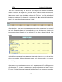
10.3 HISTORY OF CHANGES. ICCAchange.txt......................................................... 92
10.4 HISTORY OF RELEASES. ICCArelease.txt..................................................... 109
CONCLUSIONS .............................................................110
LIST OF APPENDIX ........................................................112
-6-
CERN
Industry Coil Calibration
A1.
SPÉCIFICATION
FONCTIONELLE
DE
LA
CALIBRATION
PÉRIODIQUE DES TAUPES MAGNÉTIQUES .............................113
A2. ICCA USER’S MANUAL ................................................118
A3. NMR TESLAMETER PT-2025 DATASHEET ........................ 1984
A4. PCU 2000 MAXON MOTOR CONTROL DATASHEET ................200
A5. FUG POWER SUPPLY NTN 300-60 DATASHEET ....................203
A6. INTEGRATOR AT680-2030-050 DATASHEET ......................207
BIBLIOGRAPHY .............................................................216
LIST OF FIGURES AND TABLES..........................................218
ACKNOWLEDGEMENTS.....................................................220
-7-
CERN
Industry Coil Calibration
-8-
CERN
Industry Coil Calibration
INTRODUCTION
As the LHC machine is in the construction stage and many magnets are being tested
for validation, a new system dedicated for coil calibration is required. Moles features
must be measured periodically in order to guarantee the precision of the magnetic
measurements and to follow their stability. Concretely, some of the operations that
must be carried out are the recalculation of the coils surfaces inside the mole,
verifying the parallelism between them, checking the linearity of the gravity sensor...
Industry Coil CAlibration (ICCA) system, created to satisfy these requests from
AT/MTM, is composed by a program developed in LabVIEW running in Sun
Workstations that controls some devices in a mini-rack, dedicated just for calibration
purposes, attached to DIMM and QIMM systems. This system is based on magnetic
measurements since it is the best and most direct way to verify that the expected
field properties (strength, quality and geometry) of the magnets have been reached.
It will be useful not only in dedicated benches at CERN but also in the industry.
-9-
CERN
Industry Coil Calibration
CHAPTER 1.
CERN
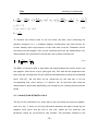
The creation of an European Laboratory was recommended at a UNESCO meeting in
Florence in 1950 and, three years later, a Convention was signed by 12 countries of the
'Conseil Européen pour la Recherche Nucléaire'. CERN was born as the prototype of a
chain of European institution in space, astronomy and molecular biology. This scientific
laboratory sites on both sides of the Franco-Swiss border west of Geneva at the foot
of the Jura Mountains.
Figure 1.1: CERN’s location.
CERN is today composed of 20 member States: Austry, Belgium, Bulgary, Czech
Republic, Denmark, Finland, France, Germany, Greece, Hungary, Italy, Netherlands,
Norway, Poland, Portugal, Slovak Republic, Spain, Sweden, Switzerland and the United
Kingdom and around 6500 scientists use CERN's facilities. [1]
CERN’s aim is to provide the European scientific community with the facilities to
probe the structure of matter and reach a better understanding of the behaviour of
- 10 -
CERN
Industry Coil Calibration
the universe, how was it created… only for scientific purpose with no immediate
technological or commercial objectives. It has been built and operated the particle
accelerators needed as means for such research in a unique centre which allows
physicists around Europe to collaborate more fruitfully than if each country
maintained an independent program. However, even in the short term this fundamental
research, with its stringent demands for accuracy and ultra-fast response, pushes
modern technology to the limit.
For high interaction energies, the laboratory has developed several fixed targets and
colliding beam machines. The first ones were the Proton Synchrotron (PS), that came
into operation in 1959 supplying fixed target experiments with 28 GeV beams of
protons, and the Intersecting Storage Rings (ISR) proton-proton collider, which began
to act in 1971. The next step was represented by the Super Proton Synchrotron (SPS)
which was later made into the proton-antiproton collider (at 450 GeV/beam energy)
which started to work in 1981. It led to the discovery of the W and Z particles (the
carriers of the weak nuclear force) confirming the elegant theory unifying
electromagnetic and weak forces (electroweak theory). This discovery by Carlo
Rubbia's team, together with the development of a new technique (stochastic cooling)
to control the anti-protons and shape them into an intense beam, by Simon var der
Meer, earned them the Nobel Prize for Physics in 1984.
Since 1989, these accelerators have also represented the elements of a chain to preaccelerate and inject electrons and their antiparticles, positrons, into the Large
Electron-Positron collider (LEP), where their energy was increased up to 46 GeV, while
bunches containing 1011 particles were made travel in opposite direction in the same
ring, before the head-on collision of two bunches occurred within a detecting unit. By
means of this machine physicists could make a detailed study of Z boson, that were
- 11 -
CERN
Industry Coil Calibration
abundantly produced at 92 GeV energy. At 1996, the LEP energy doubled, thanks to
superconducting accelerating cavities, reaching 105 GeV per beam.
Figure 1.2: The CERN network of interlinked accelerators and colliders.
1.1. HIGH ENERGY PARTICLE PHYSICS CHALLENGES
Particle physicists have found that they can describe the fundamental structure and
behaviour of matter within a theoretical framework called the Standard Model. This
model incorporates all the known particles and forces through which they interact,
with the exception of gravity. It is currently the best description we have of the
world of quarks and other particles. However, the Standard Model in its present form
cannot give answers to some questions: there are still missing pieces and other
challenges for future research to solve.
The masses of the particles vary within a wide range of masses. The photon, carrier of
the electromagnetic force, and the gluons that carry the strong force, are completely
- 12 -
CERN
Industry Coil Calibration
massless, while the conveyors of the weak force, the W and Z particles, each weight
as much as 80 to 90 protons or as much as reasonably sized nucleus. The most massive
fundamental particle found so far is the top quark. It is twice as heavy as Z particles,
and weights about the same as a nucleus of gold. The electron, on the other hand, is
approximately 350,000 times lighter than the top quark, and the neutrinos may even
have no mass at all.
Why there is such a range of masses is one of the remaining puzzles of particle
physics. Indeed, how particles get masses at all is not yet properly understood. In the
simplest theories, all particles are massless which is clearly wrong, so something has to
be introduced to give them their various weights. In the Standard Model, the particles
acquire their masses through a mechanism named after the theorist Peter Higgs.
According to the theory, all the matter particles and force carriers interact with
another particle, known as the Higgs boson. It is the strength of this interaction that
gives rise to what we call mass: the stronger the interaction, the greater the mass. If
the theory is correct, the Higgs boson must appear below 1 TeV. Experiments at
Tevatron and LEP have not found anything below 110 GeV.
Another open question is the unification of the electroweak and strong forces at very
high energies. Experimental data from different laboratories around the globe
confirm that within the Standard Model this unification is excluded [2]. When scaling
the energy dependent constants of the electroweak and strong interactions to very
high energies, the coupling constants do not unify. Grand Unified Theories (GUT)
explain the Standard Model as a low energy approximation. At energies in the order of
1016 GeV, the electromagnetic, weak and strong forces unify. One of the GUT
theories is the supersymmetry (SUSY) that predicts new particles to be found in the
TeV range. Many other GUT theories predict new physics at this energy scale.
- 13 -
CERN
Industry Coil Calibration
These and other questions like the elementarity of quarks and leptons, the search of
new quark families and gauge bosons or the origin of matter-antimatter asymmetry in
the Universe, will be addressed by CERN’s next accelerator, the Large Hadron
Collider, which is currently under construction.
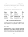
1.2. LHC
The Large Hadron Collider [3] will collide two counter-rotating proton beams at a
centre of mass energy of 14 TeV. This energy is seven times higher than the beam
energy of any other proton accelerator to date. In order to achieve an unprecedent
luminosity of 1034 cm-1s-2, it must operate with more than 2800 bunches per beam
and a very high intensity. The machine can also be filled by lead ions up to 5.5
TeV/nucleon and therefore allow heavy-ion experiments at energies about thirty times
higher than at the Relativistic Heavy Ion Collider (RHIC) at the Brookhaven National
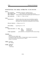
Laboratory in New York. Some of the parameters of the new accelerator are listed
below:
TOPIC
VALUE
UNITS
Energy
Injection Energy
Dipole Field
Number of dipole magnets
Number of quadrupole
magnets
Number of corrector
magnets
Luminosity
Coil aperture in arcs
Distance between apertures
Particles per bunch
Number of Bunches
7
0.45
8.36
1232
430
TeV
TeV
Tesla
8000
aprox.
1034
56
194
1011
2835
cm-2s-1
mm
mm
Table 1.1: Summary of the LHC parameters [4]
- 14 -
CERN
Industry Coil Calibration
The primary task of the LHC is to make an initial exploration of the 1 TeV range. The
major LHC detectors, ATLAS (A Toroidal LHC AparatuS) and CMS (Compact Muon
Solenoid) should be able to accomplish this for any Higgs mass in the expected range.
To get into the 1 TeV scale the needed beam energy is 7 TeV.
Together with ATLAS and CMS, two other experiments will be fed by the LHC: a
dedicated heavy ion detector, ALICE, which will be built to exploit the unique physics
potential of nucleus-nucleus interactions at LHC energies, and LHC-B, which will carry
out precision measurements of CP-violation and rare decays of B mesons.
The LHC has been prepared since the beginning of the 80’s, with a R+D program for
superconducting dipole magnets and the first design of the machine parameters and
lattice. The CERN Council approved the LHC in 1994. At that time it was proposed to
build the machine in two energy stages due to limiting funding. Strong support for LHC
from outside the CERN member states was found and CERN Council decided in 1996 to
approve the LHC to be built in only one stage with 7 TeV beam energy. Civil engineering
works for the LHC are almost completed. The series production of the magnets has
already started and works well. The prototypes String I and II have shown the
feasibility of high magnetic field cryomagnets connected in series. Installation of the
LHC components into the tunnel started after removal of LEP was completed.
Injection into first octant is foreseen for 2006. It is planned to complete the machine
installation and to start operation in 2007 [5].
1.3. LHC LAYOUT
The LHC has an eight-fold symmetry with eight arc sections and eight long straight
sections. Two counter-rotating proton beams will circulate in separate beam pipes
- 15 -
CERN
Industry Coil Calibration
installed in the same magnet (twin-aperture). The beams will cross over at the four
experiments resulting in an identical path length for each beam.
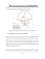
Each arc consist of 23 identical cells, giving the total length of 2465 m. Cells are
formed by six 15 m-dipole magnets and two quadrupole magnets (these dipoles and
quadrupoles are called lattice or main magnets). Dipole magnets are used to deflect
the beam whereas quadrupole magnets act as lenses to focus the beam. Different
from an optical lens, a magnetic lens focuses in one transverse direction and defocuses
in the other one. In order to obtain a net focusing effect, two quadrupole magnets are
needed (similar to the principle of Galileo’s telescope). This is a FODO-lattice, in which
F and D stand for the focusing and defocusing quadrupole. In a circular accelerator
the O stands for dipole used to bend the beam. Small dipole, sextupole, octupole and
decapole corrector magnets are installed to keep the particles on stable trajectories.
The lattice quadrupole magnets and the corrector magnets of a particular half-cell
form a so called short straight section (SSS) and are housed in a common cold mass
and cryostat.
Figure 1.3: LHC cell layout: the six main dipole magnets, two lattice quadrupoles and
correctors.
At the beginning and the end of the straight sections a dispersion suppressor cell
consisting of four quadrupoles interleaved with four strings of two dipoles each, is in
charge of correcting the orbit deviation due to the drift in the energy of the
- 16 -
CERN
Industry Coil Calibration
particles. The four long straight sections where the experiments are located, are
formed by the dispersion suppressors and the insertion magnets. These last ones quick
the separated beams to a common pipe where they are finally focused by the so called
inner triplet magnets in order to get very low beams before collisions inside the
detectors.
The other insertions are to be used by systems for the machine operation: beam dump,
beam cleaning (collimation), RF-cavities (accelerator units) and injection from
preaccelerators.
The injector complex includes many accelerators at CERN: linacs, booster, LEAR as an
ion accumulator, PS and the SPS. The beams will be injected into the LHC from the
SPS at an energy of 450 GeV and accelerated to 7 TeV in about 30 min, and then
collide for many hours.
Figure 1.4: Layout of the LHC.
- 17 -
CERN
Industry Coil Calibration
CHAPTER 2.
SUPERCONDUCTIVITY AND SUPERCONDUCTING MAGNETS
2.1. BASICS OF SUPERCONDUCTIVITY
Superconductivity is a remarkable phenomenon whereby certain materials, when cooled
to very low temperatures, become perfect conductors of electricity. From
experiments [6] it is known today that the resistivity in the superconducting state is
at least 1012 times smaller than the resistivity in the normal-conducting state.
There exist two reasons for the development of superconducting technologies within
accelerator projects: superconducting magnets allow higher particle energies for a
given accelerator size, promising a substantial saving in the operating cost of the
machine. Normal magnets with iron pole shoes are limited to dipole fields of about 2
Tesla and quadrupole gradients of 10 Tesla/m whereas with superconducting coil fields
of more than 8 Tesla and gradients in excess of 200 Tesla/m are safely accessible.
2.2. SUPERCONDUCTING MAGNETS
In a circular accelerator of ions with mass A and charge Q, the kinetic energy K is
given by the relation:
  Q 2
KK
2
+
2W

 (300BR)
0 ≈ 
  A
A A
( 2.1)
where W0 is the rest energy and B the mean magnetic field. The energies are in MeV,
the magnetic field in Tesla and the radius in meter. For a high energy proton or
electron A = 1, W0 « K so K = W and the equation above is reduced then to:
W ≈ 300BR
- 18 -
(2.2)
CERN
Industry Coil Calibration
The LHC is being installed in the 27-kilometres LEP tunnel; hence a 8.3 Tesla dipole
field is needed in order to deflect the proton beams. This magnetic field can only be
achieved at an acceptable cost using superconducting technology [4] by cooling
magnets to 1.9K with superfluid helium. The attainment of 7 TeV in the existing tunnel
presents some considerable technological challenges. The small tunnel cross section as
well as the need for cost reduction imposes a two in-one magnet design for the main
dipoles and quadrupoles. The LHC machine is, actually, two accelerators sharing the
same cryostat.
The very flexible LHC optics requires a large number of superconducting magnets,
their connections with superconducting bus bars and current leads as part of the
electrical circuits. In total, about 10,000 magnets connected within 1,700 electrical
circuits will be installed.
2.3. QUENCH
The energy stored in the superconducting magnets is very high (10 GJ in the electrical
circuits and 700 MJ in the circulating beams [4]) and can potentially cause severe
damages when the superconducting state disappears due to beam losses or cryogenic
failures. The resistive transition from the superconducting to the normal-conducting
state is called a quench. When it occurs, unless precautions are taken, the stored
magnetic energy can generate excessive voltages and overheating whose consequences
may lead to magnet degradation, a short circuit due to a melted insulation or even an
open circuit, which occurs when the conductor burns out.
A reliable active Quench Protection System (QPS) is needed to bring the current
down to zero safely when a quench occurs in order to assure the integrity of all the
superconducting elements in the machine.
- 19 -
CERN
Industry Coil Calibration
2.4. CRYOGENICS
31,000Tm of material must be spread over 27 km to below 2K in order to ensure a
superconducting state of the magnets. The most convenient way to cool helium to this
temperature is to reduce the vapour pressure above the liquid bath. When the
pressure is reduced in the heat exchanger below 20 mbar the helium, already in a
super fluid state, reaches the 1.9K operating temperature.
The bulk of the cold masses remains at atmospheric pressure and is cooled down by
the effect of exchange of heat. The machine will be cooled by eight cryoplants, each
with an equivalent capacity of 18kW at 4.5 K. Four of these will be the existing LEP
refrigerators upgraded in capacity from 12kW to 18kW and adapted for LHC duty.
The other four new plants, unlike those of LEP, will be entirely installed on the
surface, reducing the need of additional underground infrastructure. The machine
cryostats are fed from the cryogenic distribution line (QRL) that runs parallel to the
superconducting magnets. The magnets of the arcs and the dispersion suppressors of
one octant are housed in a common cryostat of diameter 914 mm, which is about 3 km
long with a cold mass of more than 5,000 Tm. The cooldown of the cold mass takes
around 14 days.
The first phase of the cool down will be carried out with nitrogen due to its operation
simplicity and, above all, its lower cost. It is estimated that about 12 million litres will
be evaporated during that phase. Afterwards, 700,000 litres of helium will be
necessary to set the whole machine at 1.9 K. The LHC will be the biggest concentration
of super fluid liquid in the Universe.
2.5. MAIN MAGNETS AT LHC
There are two main kinds of magnets composing the LHC: dipole magnets, which bend
- 20 -
CERN
Industry Coil Calibration
the beam, and quadrupole magnets that focus it. The 154 main dipoles of an arc are
powered in series whereas two independent circuits power the quadrupoles of an arc:
one for the focusing and one for the defocusing apertures. In the insertions, the
apertures of the quadrupoles are either powered individually or in series of two.
2.5.1. Main dipoles
Among the 10,000 superconducting magnets required for the LHC, the most
challenging are the 1,232 superconducting dipoles which must operate reliably at the
nominal field of 8.3 Tesla, corresponding to the centre of mass energy of 14 TeV, with
the possibility of being pushed to an ultimate field of 9 Tesla.
Two technologies for the achievement of fields above 9 Tesla were investigated
before the development and construction of dipoles for the LHC: One that uses
Nb3Sn at 4.2 K and another one with NbTi technology at reduced temperature. With
the first technology a dipole model with a first quench at 11 Tesla was successfully
built in Twente University but the coils manufacture’s difficulty and the high economic
cost makes its use unfeasible. The other more economical alternative, however,
suffers from the drawback that the specific heat of the superconducting material and
its associated copper matrix falls rapidly as the heat temperature is reduced. This
makes the coil much more premature to quenches due to small frictional movements of
conductor strands or particle losses.
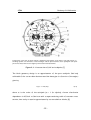
The cross section of the twin-aperture LHC dipole magnet is shown in the picture
below. The coil has a 6-block geometry design which optimizes the field quality and
allow more flexibility for small changes during series production.
- 21 -
CERN
Industry Coil Calibration
1-beam tube; 2-SC coils, “6-block” design; 3-austenitic steel collars; 4-iron yoke; 5-iron yoke “insert”, 6shrinking cylinder / He II vessel; 7-heat exchanger tube; 8-dipole bus-bars; 9-arc quadrupole and “spoolpieces” bus-bars; 10-wires for magnet protection and instrumentation.
Figure 2.1: Cross-section of LHC series dipoles [7]
The block geometry design is an approximation of the pure multipole field only
achievable if the current distribution around the beam pipe is a function of the angle φ
given by:
I(φ) = I0 cos(mφ)
(2.3)
where m is the order of the multipole (m = 1 for dipoles). Current distribution
dependence is difficult to fabricate with a superconducting cable of constant crosssection; that is why it must be approximated by current shells or blocks. [8]
- 22 -
CERN
Industry Coil Calibration
The force containment structure consists in coil clamping elements: the steel collars,
the iron yoke, the iron insert and the steel shrinking cylinder that contribute to keep
the coils in their nominal position. The shrinking cylinder is also the outer shell of the
helium tank. This cold mass is 15 m long and 23.8 Tm heavy.
The parameters of the LHC main dipole magnets are summarized in this table:
TOPIC
Magnetic length
Total length
Operating temperature
Stored energy
Current at injection
JNbTi inner layer 7 TeV
JNbTi outer layer 7 TeV
Bending radius
Number of beams/magnet
Coil inner diameter
Coil outer diameter
Mass and cold mass
VALUE
14.3 m
15180 mm
1.9 K
7.1 MJ
739 A
1200 A/mm2
1732 A/mm2
2803.928 m
2
56 mm
120.5 mm
23.8Tm
TOPIC
Nominal current
Coil length
Peak field in coil
Field at injection
Field at 7 TeV
Number of turns inner layer
Number of turns outer layer
Bending angle per magnet
Number of blocks and layers
Inductance per magnet
Cable length for inner layer
Cable length for outer layer
VALUE
11796 A
14567mm
8.76 T
0.53 T
8.33 T
2 x 15
2 x 26
5.1 mrad
6 and 2
0.108 H
433 m
751m
Table 2.1: The main parameters of the LHC dipole magnets [9].
The main dipoles are classified into type A (MBA) and type B (MBB) depending on the
electrical connections and the corrector magnets they host. They are alternately
located along the arc in order to get a balanced-inductance circuit.
2.5.2. Main quadrupoles
The main quadrupole magnets for the LHC are the twin aperture or lattice quadrupoles
(MQ) and the insertion quadrupoles (MQM family, MQY and MQX magnets). The MQ
quadrupoles provide the field to focus the particle beam and to keep it near the
reference orbit. The LHC will feature 360, 3.25m long lattice quadrupoles, designed
- 23 -
CERN
Industry Coil Calibration
for a 223 Tesla/m gradient field.
The main parameters of these magnets are listed in the following table:
TOPIC
VALUE
TOPIC
VALUE
Magnetic length
3.10 m
Nominal Current
11,870 A
Peak field in coil
6.86 Tesla
Current at injection
763A
Gradient at injection
14.3 Tesla/m
Coil inner diameter
56 mm
Nominal gradient
223 Tesla/m
Coil outer diameter
118.6 mm
Geometrical aperture
56 mm
Coil length
3,184 mm
Inductance per magnet
0.0112H
Number of coil layers
2
Stored energy
0.784 MJ
Number of turns per pole
24
Max. rating current
13 kA
Cable length per pole
160m
Current density 7 TeV (NbTi)
1789 A/mm2
Total cable length
1280m
Table 2.2: The main parameters of the MQ magnets [9]
Unlike the main dipoles, the two coils sharing the same cryomass on the quadrupoles
are powered by independent circuits that shift aperture every magnet in such a way
that when the beam is horizontally focused in one aperture it is vertically focused
(hence horizontally defocused) in the neighbour aperture. Moreover, the current
bypasses every second magnet in order to get a balanced circuit.
The main lattice quadrupoles are housed in the so-called Short Straight Sections
(SSS), they also contain several other kinds of magnets (namely octupole, dipole and
sextupole correctors, tuning quadrupoles and skew quadrupoles), the protection diodes
and the beam position monitors. The other group of main quadrupole magnets is the
one used in the insertion for the experiments.
- 24 -
CERN
Industry Coil Calibration
Figure 2.2: Cold mass cross section of the LHC short straight section [10]
2.5.3. Correctors
The corrector magnets of the LHC are smaller than main dipoles or quadrupoles. They
are wound with single strand cables and the coils are fully impregnated with epoxy,
which reduces the cooling by helium. In order to achieve the field quality, sextupole
(MCS), octupole (MCO) and decapole (MCD) magnets (spool piece corrector magnets)
are installed at the ends of the main dipole magnets correcting the multipole field
errors. Every aperture of each dipole magnet is equipped with a sextupole corrector
coil, whereas only every second dipole magnet (type B) will be equipped with octupole
and decapole correctors.
The sextupole magnets (MS, MSS) correct the chromaticity and the quadrupole
- 25 -
CERN
Industry Coil Calibration
magnets (MQT, MQS, MQTL) compensate coupling between the transverse planes and
adjust the betatron tune (number of oscillations of the beam around the central orbit
per turn). Lattice octupole magnets (MO) will be installed to adjust other beam
parameters.
About 1,000 small dipole magnets (MCB in the arcs and MCBC, MCBR, MCBX, MCBY in
the insertions) will be installed to correct the particle trajectory in both transverse
planes, the closed-orbit corrector magnets. All the superconducting corrector
magnets of the same type located in the same aperture of an arc are powered in series
at a nominal current of 120A for MCO and 550A for the rest. The dipole correctors
are powered individually with nominal currents from 60A to 600A depending on their
function. [11]
- 26 -
CERN
Industry Coil Calibration
CHAPTER 3.
AB/CO/IS/LS SECTION
CERN is divided into several departments (antique divisions) each one dedicated to
different tasks. As well, these departments are divided into groups and then into
sections and subsections.
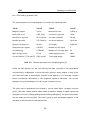
AB department (Accelerator Beam) hosts the groups responsible for beam generation,
acceleration, transfer, control and delivery for the CERN accelerator complex. It is
responsible for the specification, procurement and commissioning of the equipment for
the above systems for the LHC machine, as well as for the power converters for the
LHC detectors.
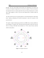
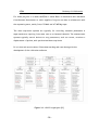
AB/CO group (COntrol) has been created in January 2003. It is responsible for all the
controls infrastructure of all the accelerators of CERN. More than 110 people are
working in this group to maintain the running installed base but also to study, define,
develop and deploy the future control elements that will be used for the future LHC
accelerator.
AB/CO/IS section (Industrial Systems), previously called LHC/IAS, has as main
functions the definition, selection and implementation of industrial control and
supervision systems for the LHC machines equipment, including cryogenics. It also
contributes CERN-wide consultancy and support for promoting convergence in
industrial control.
AB/CO/IS/LS
[12]
(Laboratory
Systems)
sub-section’s
main
activities
are
concentrated on data acquisition and measurement systems for LHC components or
assemblies, either to be used at CERN or the manufacturer’s production site.
- 27 -
CERN
Industry Coil Calibration
For these projects it is used LabVIEW or Visual Basic in combination with hardware
from National Instruments or other suppliers. Projects are done in collaboration with
the requesting users, mainly from AT/MAS and AT/MTM groups.
The data acquisition systems are typically for recording transient phenomena in
superconductors requiring from some tens to a thousand channels. The measurement
systems typically control devices to vary parameters, such as current, rotation or
displacement of probes, with synchronised data acquisition.
It is in this sub-section where I have been working and contributing with the
development of the calibration software.
Figure 3.1: AB/CO organigram [13]
- 28 -
CERN
Industry Coil Calibration
CHAPTER 4
MAGNETISM PRINCIPLES
To understand how the data from the magnetic measurements system, used in the
magnetic measurement program included in ICCA application, is acquired and treated,
it is important to define, firstly, the analysis procedure used to achieve them.
Moreover, some definitions and relations about magnetism are shown. [14 .. 20]
4.1. MAGNETIC FIELD AND FLUX DEFINITIONS
In order to understand the way the magnetic measurements system for calibration
works, it is important to begin defining some of the important laws and equations
related to magnetism.
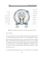
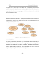
4.1.1. Magnetic field
Magnetic fields are produced by electric currents, which can be macroscopic currents
in wires, or microscopic currents associated with electrons in atomic orbits. The
magnetic field B is defined in terms of force on moving charge in the Lorentz force
law. The interaction of magnetic field with charge leads to many practical applications.
Magnetic field sources are essentially dipolar in nature, having a north and south
magnetic pole.
Figure 4.1: Magnetic field sources
- 29 -
CERN
Industry Coil Calibration
Figure 4.2: Magnetic field’s tree
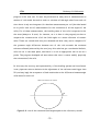
4.1.2. Magnetic Flux
Magnetic flux is the product of the average magnetic field times the perpendicular
area that it penetrates. It is a quantity of convenience in the statement of Faraday's
Law and in the discussion of objects like transformers and solenoids. In the case of an
electric generator where the magnetic field penetrates a rotating coil, the area used
in defining the flux is the projection of the coil area onto the plane perpendicular to
the magnetic field.
r r
∂ψ = B ⋅ ∂S
(4.1)
[ψ] = T ⋅ m 2 = Wb
The contribution to magnetic flux for a given area is equal to the area times the
component of magnetic field perpendicular to the area. For a closed surface, the sum
- 30 -
CERN
Industry Coil Calibration
of magnetic flux is always equal to zero (Gauss' law for magnetism). No matter how
small the volume, the magnetic sources are always dipole sources (like miniature bar
magnets), so that there are as many magnetic field lines coming in (to the south pole)
as out (from the north pole).
4.1.3. Maxwell’s equations
Maxwell's equations represent one of the most elegant and concise ways to state the
fundamentals of electricity and magnetism. From them one can develop most of the
working relationships in the field.
Figure 4.3: Maxwell’s equations’ tree
4.1.4. Faraday’s law
Any change in the magnetic environment of a coil of wire will cause a voltage (emf) to
be "induced" in the coil. No matter how the change is produced, the voltage will be
generated. The change could be produced by changing the magnetic field strength,
moving a magnet toward or away from the coil, moving the coil into or out of the
magnetic field, rotating the coil relative to the magnet, etc.
- 31 -
CERN
Industry Coil Calibration
Faraday's law is a fundamental relationship which comes from Maxwell's equations. It
serves as a succinct summary of the ways a voltage (or emf) may be generated by a
changing magnetic environment. The induced emf in a coil is equal to the negative of
the rate of change of magnetic flux times the number of turns in the coil. It involves
the interaction of charge with magnetic field.
emf = − N t
[emf ] = V
∂ψ
∂t
(4.2)
Figure 4.4: Faraday’s law tree
4.1.5. Lenz’s law
When an emf is generated by a change in magnetic flux according to Faraday's Law,
the polarity of the induced emf is such that it produces a current whose magnetic
field opposes the change which produces it. The induced magnetic field inside any loop
of wire always acts to keep the magnetic flux in the loop constant. In the examples
below, if the B field is increasing, the induced field acts in opposition to it. If it is
decreasing, the induced field acts in the direction of the applied field to try to keep it
constant.
- 32 -
CERN
Industry Coil Calibration
4.1.6. Lorentz’s force law
Both the electric field and magnetic field can be defined from the Lorentz force law:
r
r
r r
F = qE + qv xB
r
E : electric force
r
B : magnetic force
(4.3)
The electric force is straightforward, being in the direction of the electric field if
the charge q is positive, but the direction of the magnetic part of the force is given
by the right hand rule.
Figure 4.5: Electric and magnetic force
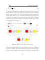
4.1.7. Equations in the system
The magnetic measurements system works in the following way. A constant magnetic
field is created while setting current to a magnet (dipole or quadripole). The features
of this magnetic field (absolute value, angle, harmonics…) are really important to know
since they explain with precision how particles can be deflected, focused by Lorentz’a
force… into the accelerators. Probes, a set of coils, are needed for this purpose; as
they present an area the magnetic flux can be measured once they are inserted into
the magnet. From equation (4.1):
- 33 -
CERN
Industry Coil Calibration
r r
ψ = ∫ B ⋅ ∂S = B S cos(α )
s
(4.4)
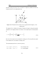
The amount of flux depends on the angle that relates the surface vector with the
magnetic field vector. This is to say, depends on the orientation of the coils inside the
magnet. In order to sweep all the flux increments along the different positions the
coils may adopt (a whole turn), they are rotated inside the magnetic field while, due to
Faraday’s law, the voltage from the coils are read. With this procedure, and with some
mathematical relations (multipole expansion of the magnetic field (4.2.1)), any data can
be reconstructed. From equation (4.2):
1
∫ V (t)∂t; ∫ V (t)∂t = −N t BS cos(α);
Nt
∂α
∂t =
; α ∈ 0..2π
ω
ψ=−
∫ cos(α) ∂α = −ωN
V (α)
t
B S;
(4.5)
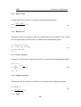
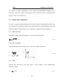
Figure 4.6: Magnetic flux and angle of rotation relation
Voltage delivered by the coil is not the same in these three cases since it depends on
the amount of magnetic field vectors that goes through the coil area: the magnetic
flux. This is to say, it depends on the coil’s position with respect to the magnetic field.
- 34 -
CERN
Industry Coil Calibration
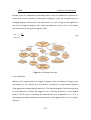
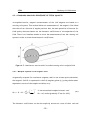
4.2. STANDARD ANALYSIS PROCEDURE OF FIELD QUALITY
As explained earlier, magnetic measurements of the LHC magnets are based on a
rotating coil system. This method delivers a measurement of the magnetic flux linked
with the coil as a function of angular position. Also, the main quantities of interest for
field quality characterization are the harmonic coefficients of the expansion of the
field. There is a formalism needed to treat the measurements from the rotating coil
system in order to obtain these harmonic coefficients.
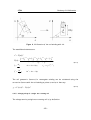
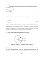
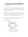
Figure 4.7: Head sector section with five radial rotating coils in a dipole field
4.2.1. Multipole expansion of the magnetic field
As generally accepted for accelerator magnets, and for use in beam optics simulation,
the magnetic field B is expressed in the 2-D imaginary plane (x,y) using the harmonic
expansion in terms of the complex variable z=x+iy :
 z
B ( z ) = B y + iBx = ∑ Cn 
 Rref
n =1
∞



n −1
Cn: non-normalized complex harmonic coef.
(4.6)
Rref: ref. radius (presently 17 mm for LHC).
The harmonic coefficients can be also explicitly written as a sum of their real and
- 35 -
CERN
Industry Coil Calibration
imaginary parts. The normalized coefficients, after a normalizing procedure that
depends on the magnet function, are obtained for a normal magnet of order m (m=1 for
dipole) using:
Bm : main magnetic field.
104: factor to produce practical units.
B
C
A 
cn = 10 4 n = 10 4  n + i n  = bn + ia n
Bm
Bm 
 Bm
Cn expressed in so called units.
(4.7)
bn: normal component of the 2n-pole.
an: skew component of the 2n-pole.
4.2.2. Transformation of harmonic coefficients
Two relations among the harmonic coefficients are needed to describe a rigid
translation of the reference frame in the 2-D complex plane by a vector ? z=? x+i? y,
and a rotation of the reference frame by an angle θ. They are derived from the
invariance of the magnetic field:
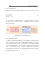
4.2.2.1. Reference frame translation
If the reference frame is translated by ? z, the harmonic coefficients Ck (in the
original system x,y) transform into C’n (in the translated system x’,y’) according to:

(k − 1)!   ∆z 
C'n = B'n +iA'n = ∑
Ck 

k =n  (n − 1)!(k − n)!   Rref 
n ≥1
∞
k −n
- 36 -
(4.8)
CERN
Industry Coil Calibration
Figure 4.8: Translation of the reference frame
4.2.2.2. Reference frame rotation
If the reference frame is rotated by and angle θ, the harmonic coefficients Cn (in the
original system x,y) transform into C’n (in the rotated system x’,y’) according to:
C'n = B'n +iA'n = Cn e in
(4.9)
Figure 4.9: Rotation of the reference frame
4.2.3. Principle of measurement with a single turn rotating coil
The measurement by a rotating coil delivers the change of the magnetic flux linked
- 37 -
CERN
Industry Coil Calibration
with the rotating coil surface. This is a model for a single turn, slender coil with two
filaments normal to the complex plane (x,y) :
Figure 4.10: Filaments location, normal to the (x,y) plane and with length L, in the
complex plane.
The magnetic flux ψ linked by the couple of filaments of length L (along the ignorable
dimension of the magnet) located at z1 and z2 in the complex plane can be expressed
as:

z2

∞ 1
ψ = LRe  ∫ B ( z )dz  = LRe ∑ n −1 Cn ( z 2n − z1n ) 

 n =1 nRref

 z1
(4.10)
Note that this formula can be extended for winding coils. The only difference would
be the addition of Nt, the number of winding turns.
The instantaneous position in a rotation is given by:
z1 ( t ) = z1 (0) e iθ ( t ) = R1e iθ1 ( t ) e iθ ( t )
R 1, R2: Filament radii.
z 2 (t ) = z 2 ( 0) e iθ ( t ) = R2 e iθ2 ( t ) e iθ ( t )
θ1, θ2: Initial phases.
- 38 -
(4.11)
CERN
Industry Coil Calibration
With these two expressions, rewritten in term of the average initial phase θ0, it is
obtained:
z − z = (R e
n
2
n
1
n inθ 2
2
−R e
n inθ 1
1
)e
inθ
∆θ 
 n in ∆θ
−in
n
2
=  R2 e
− R1 e 2 e inθ 0 e inθ


θ0 =
θ1 + θ2
2
(4.12)
∆θ = θ2 − θ1
With which, the magnetic flux equation can be compacted as follows:
 ∞ χn

ψ (θ ) = LRe ∑ n −1 Cn e inθ 
 n =1 nRref

χn: coil geometric factors
(4.13)
The complex coil geometric factors are related to the coil sensitivity factors of order
n by the expression:
∆θ
∆θ

in
−in

χ n =  R2n e 2 − R1n e 2  e inθ0


(4.14)
This form above describes the rigid rotation of an ideal coil around its axis, without
variations of the radii and of the opening. This means that the phase θ changes
periodically throughout the rotation whereas the coil geometric factors χn remain
constant.
4.2.4. Rectangular coil winding
Up to now, all the equations have been referred to a couple of filaments that is not
the real case since rectangular coil winding are used for the measurements. In this
case, a correction factor to each side of the coil winding, which will correspond to the
relation between the filament approximation and the rectangular approximation, must
be applied. This correction is equivalent to the average of the filament approximation
over the rectangular 2? x52? y rotated from the tangent by an angle α. [21]
- 39 -
CERN
Industry Coil Calibration
Figure 4.11: Rotation of the coil winding with tilt
The established relations are:
z rn = Γr (α)z fn
(1+ ξ)
n+ 2
Γr (α) =
ξ=
ξ* =
∆z
;
zα
∆z *
;
za
− (1+ ξ * )
n+ 2
+ (1− ξ)
n+ 2
− (1− ξ * )
n+ 2
(n +1)(n + 2)(ξ 2 + ξ *2 )
∆z = ∆x + i∆y;
(4.15)
−i θ −α
zα = z f e ( f )
∆z * = ∆x − i∆y;
The coil geometric factors for rectangular winding can be calculated using the
correction factors with the coil winding at points z 1 and z2 in that way:
χ n = Γr 2 (α2 )z 2n − Γr1(α1)z1n
(4.16)
4.2.5. Voltage pickup of a single turn rotating coil
The voltage seen by a single turn rotating coil is, by definition:
- 40 -
CERN
V =−
Industry Coil Calibration
∞ 1
 ∂ Cn
∂ψ
∂θ 
= −LR e ∑ n−1 χ n e inθ 
+ inC n 
 ∂t
∂t
∂ t 
 n=1 nRref
(4.17)
As seen, the voltage is induced both by a variation of the field and by a rotation of
the coil.
4.2.6. Relation between discretely sampled fluxes and harmonic coefficients
The value of the magnetic flux in each rotating coil measurement is expressed in
function of the rotation angle θk in a discrete series of points k for a total of N points.
The sampling points are equally spaced over the [0...2p] interval, and the set of
sampled points that composes the magnet flux is indicated as ψk. To reconstruct the
harmonic coefficients it is used a discrete Fourier transform (DFT) defined as:
N
ψn = ∑ψ ke
−2πi( n−1)
n =1... N
(k−1)
N
ψ : DFT complex coefficients
n
ψ : DC component
1
k=1
(4.18)
And then, the inverse DFT signal reconstruction is given by:
1
ψk =
N
N
∑ψ e
n =1
2πi ( k −1)
( n −1)
N
n
(4.19)
k =1... N
It is possible to establish a relation between the DFT coefficients and the field
harmonic coefficients Cn. This relation, for an even number of points N and valid for a
single turn idealized coil, is given by:
n −1
2 1 nRref
Cn ≈
ψ n+1
N L χn
n =1...
N
(4.20)
2
- 41 -
CERN
Industry Coil Calibration
4.2.7. Coil sensitivity
In the case of an ideal coil wound with Nt turns (with negligible winding size), the
previous relation can be rewritten in the following form:
n −1
2 Rref
Cn ≈
ψ n+1
Nt κ n
n = 1...
N
(4.21)
2
where the coefficients kn are the complex coil sensitivity coefficients to the harmonic
of order n which are proportional to the coil geometric factors χn introduced earlier:
κn =
N t Lχn
n
(4.22)
These factors completely describe the geometry of the coils into the mole
coordinates and, as said earlier, are independent of the magnetic field. The coil
sensitivity is in general a complex number but there are two important, particular
cases: that of a radial, where this coil sensitivity is a real number, and of a tangential
coil, imaginary number.
κnradial =
NtL n
R2 − R1n)
(
n
κntangential =
2iN t L n  n∆θ 
R sin

 2 
n
(4.23)
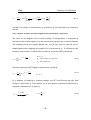
Figure 4.12: Radial and tangential coil and complex coil sensitivity factors.
- 42 -
CERN
Industry Coil Calibration
These two cases refer to a single coil reading the magnetic flux, what is called an
absolute measurement used to determine the main field component. But there is also
the so called compensated measurement done by connecting different coils with
appropriate gains in order to cancel the main field component and, hence, to reach a
better radio signal/noise. To obtain the total sensitivity coefficients kn to an harmonic
n from a set of S coils with different sensitivities each one it is used this expression:
κ
S
cmp
n
= ∑ g sκ nS
(4.24)
s =1
gs: gain of the S th coil.
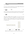
Figure 4.13: Coil sensitivity calculation scheme
Summarizing, for the calculation of the coil sensitivity of the compensated coil set the
different sensitivities of each single coil and the gains used for their signals are
needed.
- 43 -
CERN
Industry Coil Calibration
4.2.8. Coil data
The known data about the coil, from drawing, that will be useful to calculate the
sensitivity factors of a given coil are the following ones:
-
The magnetic surface S.
-
The inner length Lin.
-
The inner width W in.
-
The thickness T of the groove.
-
The number of turns Nt.
-
The contraction factor c (usually c=0.9975 for temperature ≤ 70° K).
-
The radius r 0 from the center of rotation to the magnetic center
z0 = r0eiθ 0 .
-
The relative parallelism ϕp of the coil with respect to the other coils.
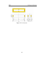
Figure 4.14: Coil positions into the head sector
- 44 -
CERN
Industry Coil Calibration
Figure 4.15: Coil dimensions
- 45 -
CERN
Industry Coil Calibration
CHAPTER 5.
STANDARD ANALYSIS OF RAW DATA
In order to generate tables of harmonic coefficients for each measurement, a
standard procedure is followed. [14 .. 20]
5.1. NON-NORMALIZED HARMONICS FROM DC MEASUREMENTS
These operations are used for the standard analysis of measurements taken in DC
conditions (with constant current in the measured magnet).
5.1.1. Pulse time
Compute the time of the trigger pulse from the angular encoder, for absolute and
compensated signals, forward and backward rotations:
t1 = 0 ( s)
t k +1 = t k + ∆t k = t k +
∆τ k
( s)
f
(5.1)
f = 106 ( Hz) f of the referenceclock for the integratorcounter and for presentintegrators.
k = 1.. N
5.1.2. Conversion
Convert the raw flux increments from integrator ? ϕ [counts] to ? ψ [Vs], for absolute
and compensated signals, forward and backward.
∆ψ k =
∆ϕ k
(Vs)
K
(5.2)
K = VFC ⋅ Gint ⋅ Gamp (countsVs)
k = 1.. N
- 46 -
CERN
Industry Coil Calibration
5.1.3. Coil Voltage and coil voltage offset
The average voltage picked up by the rotating coil during an angular step is calculated
directly from the fluxes increments and the time interval as delivered by the
integrators:
∆ψ k
(V )
∆t k
k = 1...N
Vk = −
(5.3)
Compute the voltage offset, invariable during the measurement and caused by the
cable connections and amplifier stages, for absolute and compensated signals, forward
and backward rotations.
N
Voff = −
∑ ∆ψ
k
k =1
(V )
tN+1
Vk = Vk − Voff (V )
(5.4)
5.1.4. Drift correction
Correct the flux increments for the voltage offset, for absolute and compensated
signals, forward and backward rotations.
∆ψ k = ∆ψ k + Voff ∆t k (Vs)
∆ψ k = ∆ψ k −
(5.5)
∆t k N
∑ ∆ψ k (Vs)
t N +1 k=1
k = 1.. N
- 47 -
CERN
Industry Coil Calibration
5.1.5. Signal average
Average the flux increments, for absolute and compensated signals.
∆ψ kfor − ∆ψ kback
(Vs)
2
k = 1.. N
∆ψ k =
(5.6)
5.1.6. Magnetic flux
Integrate the flux increments, which are proportional to the magnetic flux change
over an angular step of the encoder, for absolute and compensated signals.
ψ1 = 0 (Vs) → θ1 = 0 (rad)
ψ N +1 = 0 (Vs) → θ 2π = 0 (rad)
ψ k +1 = ψ k + ∆ψ k (Vs)
k = 1.. N
(5.7)
5.1.7. Fourier transform
Frequency transform the integrated flux (DFT), for absolute and compensated signals.
0 ≤ k ≤ N −1
N
ψn = ∑ψ k e
−2πi(n−1)
(k−1)
N
(5.8)
(Vs)
k=1
n = 1... N
5.1.8. Amplitude spectrum
Fold spectrum of the frequency transform, for absolute and compensated signals.
N = 2K; K ∈ Z +
ψ n +1 + ψ N* − n +1
(Vs)
N
n = 1.. N 2 −1
(5.9)
Ξn =
( )
- 48 -
CERN
Industry Coil Calibration
N = 2K +1; K ∈ Z +
ψ n+1 + ψ N* −n+1
Ξn =
(Vs)
N
n = 1.. N -1 2
(
(5.10)
)
5.1.9. Harmonics
Compute field harmonics, for absolute and compensated signals.
n−1
Rref
Cn ≈
Ξn
κn
n = 1... N m
(5.11)
After all these calculations, the results are the non-normalized field harmonics in the
reference frame of the rotating coil where the number of harmonic components
retained, Nm, is typically 15. All operations on the compensated signal are possible only
when the compensated signal is read-out; otherwise, they are skipped.
5.2. FEED-DOWN CORRECTION AND CENTER LOCATION
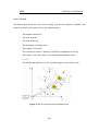
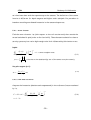
Figure 5.1: Definition of the magnetic centre coordinates
The measuring coil is in general not centred with respect to the magnetic centre of
the magnet under measurement. Through the feed-down removal procedure, all the
measurements are referred to the magnetic centre instead of the rotating coil centre
- 49 -
CERN
Industry Coil Calibration
as it has been done with the equations up to the moment. The definition of the centre
location is different for dipole magnets and higher order multipole. Its procedure is
based on cancelling non-allowed harmonics in the measured spectrum.
5.2.1. Centre location
Find the centre location ? z (with respect to the coil rotation axis) that cancels the
normal and skew 16-pole (order n=8 or/and n=10). These harmonics should be close to
zero by symmetry but can be high enough to be little influenced by fabrication errors.
Dipole:
k− n

(k −1)! C  ∆z  = 0 → seven complex roots.
∑ (n −1)!(k − n)! k  R 
  ref 
k= 8 
15
7
'
C2k
k= 4
C2k +1
f (∆z) = ∑
(5.12)
→ function to be minimized (by one of the seven roots, the center).
2m-pole magnet (m>1):
∆z = −
Rref Cm −1
(m)
m− 1 Cm
(5.13)
5.2.2. Feed-down correction
Compute the harmonics (absolute and compensated) in the reference frame translated
by ? z.

(k −1)! C  ∆z
C'n = B' n +iA'n = ∑
 k
 Rref
k= n  (n −1)!(k − n )!
n = 1... N m
∞



k−n
- 50 -
(5.14)
CERN
Industry Coil Calibration
The result of these calculations is the centred non-normalized harmonics (in a
reference frame with origin in the magnet centre), and the centre coordinates with
respect to the coil rotation axis.
5.3. NORMALIZED HARMONICS
In order to obtain normalized harmonics in units, the non-normalized harmonics must
be rotated in the reference frame of the main field first, and normalized to the main
field afterwards. The procedure to be followed for a general 2m-pole magnet is:
5.3.1. Main field value
Compute from the absolute harmonics, the main field module. |Cm|.
Cm =
Bm2 + Am2 (T )
(5.15)
5.3.2. Main field phase
Compute the phase of the main field ϕm from the absolute harmonics.
eiϕ =
Bm − iAm
Cm
[
ϕ m ∈ − π ... π
2
2
(5.16)
]
5.3.3. Angle
Compute the direction of the main field αm with respect to the measurement
reference frame.
αm =
ϕm
(rad)
m
(5.17)
- 51 -
CERN
Industry Coil Calibration
5.3.4. Rotation
Compute the non-normalized harmonics in the reference frame of the main field,
rotating them by αm.
Cn' = Bn' + iAn' = Cn e inα m (T )
(5.18)
5.3.5. Normalization
Compute the normalized harmonics of order n higher than the main field order m.
Cn
(units)
Bm
B
bn = 104 n (units)
Bm
A
a n = 104 n (units)
Bm
n = m +1... N m
cn = 104
(5.19)
The results of this procedure are rotated harmonics (absolute and compensated),
normalized to the main field for all orders higher than m. Note that the harmonic of
order m has no skew (imaginary) part because of the rotation.
5.4. RECORD OF HARMONICS
The compensated harmonics contain in principle no component below the main field
order m (as the compensation ideally cancels these components). On the other hand
the absolute harmonics have a large component at the main field order m and possibly
lower orders (due to feed-down) that may pollute the quality of the higher order
harmonics. Therefore the standard measurement result should use the absolute
- 52 -
CERN
Industry Coil Calibration
harmonics up to order m and the compensated harmonics from there on (if present).
Furthermore, through the feed-down correction and the rotation in the main field
reference frame some of the harmonics are cancelled by definition. The information
on centre location and angle must be therefore added to the final harmonic record.
- 53 -
CERN
Industry Coil Calibration
CHAPTER 6.
ICCA SYSTEM
ICCA means Industry Coil Calibration. It is a system based on magnetic measurements
and with the purpose of calibrating coil features inside the moles that are used as
probes in the process of testing and checking field properties generated by magnets.
ICCA application has been developed in LabVIEW using a standard industrial control
system so that it could be fitted in both DIMM and QIMM systems perfectly [*].
The program, extensively documented, has been designed to be easy to use at the
manufacturers’ sites by non-specialist personnel, with the minimum support from
CERN. Due to the fact that industry has experience with this kind of systems and the
final program for calibrating coils uses some already existing panels and procedures, it
requires simple maintenance.
There are available some benches and mini-racks dedicated for calibration purposes
exclusively. A power supply, a position control unit and a NMR Teslameter compose it.
These three devices will substitute the existing ones in DIMM and QIMM systems
while the calibration process. In the software point of view, there are some
differences while dealing with one or another system since some of the hardware
components (electronic cards for the levelling) and some of the measuring procedures
(number of apertures) are not the same.
[*]
DIMM means Dipole Industry Magnetic Measurements whereas QIMM,
Quadrupole Magnetic Measurements. These are two similar systems composed by
hardware
(a
rack
with
all
the
essential
components
for
making
magnetic
measurements) and software (MMP: Magnetic Measurement Program) used for
achieving and reconstructing field features for dipoles and quadrupoles magnets
respectively.
- 54 -
CERN
Industry Coil Calibration
6.1. ICCA´s ARCHITECTURE
Since the calibration procedure will be used in both DIMM and QIMM systems and it
cannot be understood without any of them, there is not unique hardware architecture
with respect to ICCA. This means that the rack destined for calibration, contributing
with its own devices, must fit the existing ones. The two different ways of presenting
the calibration system are the detailed below.
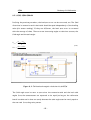
Generically, the system has a centralized architecture based on a VME industrial
standard bus connected via a fast connection card (SUN/PCI-MXI card <-> VMEMXI/VME card/VME crate) to a SUN workstation, that controls and synchronizes
every instrument involved in the measurements, running a LabVIEW application. The
VME contains ADC cards to measure the electronic gravity sensor output, the value of
current during the measurements (although finally the current will be read via GPIB
since it will be constant) and the temperature of the mole, digital I/O cards that
control the pneumatic brake and integrators to store the voltage values. The
LabVIEW application also controls the magnet power supply.
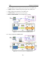
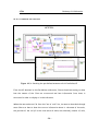
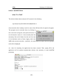
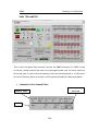
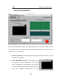
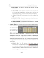
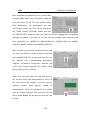
6.1.1. ICCA’s architecture in QIMM systems
QIMM systems are used for acceptance tests to quadrupole magnets in industry
during their assembly. They have got a simple structure and the hardware that
composes this dedicated rack is the following:
§
1 SUN Workstation: CPU that controls all the system thanks to the LabVIEW
software implemented. Sunmms9 in I8 will be used for calibrating moles.
§
2 INTEGRATORS: Store the absolute and compensated values from the
measurement. Into a VME crate.
§
1 ADC: Reads the current from the power supply in a more accurately way (instead
- 55 -
CERN
Industry Coil Calibration
of using a DVM) and also the angle from the level motor. Into a VME crate.
§
1 DIGIO: Enables or disables the different brakes. Into a VME crate.
§
1 CPU: For Real time Acquisistion. Into a VME crate.
§
1 POWER SUPPLY: Sources current to the system.
§
SIGNAL CONDITIONING: For the Temperature, Levelling,
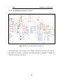
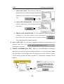
Figure 6.1: ICCA’s architecture in QIMM systems
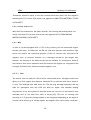
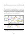
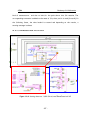
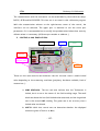
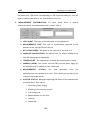
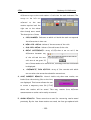
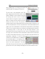
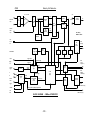
6.1.2. ICCA’s architecture in DIMM systems
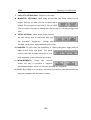
Figure 6.2: ICCA’s architecture in DIMM systems
- 56 -
CERN
Industry Coil Calibration
DIMM systems, unlike QIMM systems, are prepared to carry out magnetic
measurements with two apertures at a time. Their structure is, then, a little more
complicated since not only some extra hardware cards must be connected to the VME
bus but also because some new devices are needed for measuring the whole length of
dipoles. Nevertheless, only one-aperture measurements are taking place while
calibrating the moles.
The list of hardware components of the DIMM rack independently of the ones that
may be added with the calibration rack is:
§
1 SUN Workstation: CPU that controls all the hardware by means of the
LabVIEW software implemented.
§
1 DAC: D/A card that drives the two coil motors rotations.
§
4 INTEGRATORS: Store the absolute and compensated values generated by the
magnetic measurements from the 2 different apertures.
§
1 ADC: Acquires the level value from the two different apertures. Also, it stores
the length of the coil into the magnet.
§
2 DIG-I/O: These cards are used for the levelling motor for one, the other or
both apertures. Identically, for the pressure valves to set the brakes.
§
2 POWER SUPPLIES: There is one for the main dipole and another one when
correctors are measured.
§
2 DVM: Instead of an extra ADC card as it is used in the QIMM system for
reading in an accurately way the current from the power supply, a DVM is used for
this purpose. Two in this case as there are two power supplies.
§
1 PULLING MOTOR: Pulls the mole into the 15 m. long magnets to make
measurements along different sections inside the magnet.
§
1 LENGTH ENCODER: Measures the distance between the mole position into the
magnet and a reference final point.
- 57 -
CERN
Industry Coil Calibration
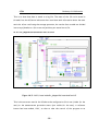
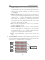
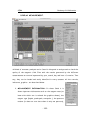
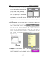
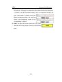
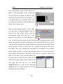
6.2. ICCA’s BENCH
The list of devices that can be found in the yellow bench and in the rack linked to
ICCA system, including the accessories inside the moles, are explained below. They are
installed and ready to be used in the Meyrin site in building 181, in I8.
Figure 6.3: ICCA’s rack and bench
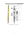
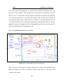
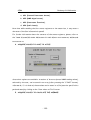
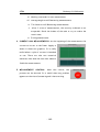
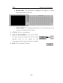
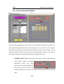
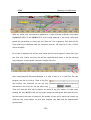
6.2.1. Reference magnet
This is the magnet that will create the magnetic field to be measured. Since it is only
used for calibration purposes, it is not superconducting and it is not used for bending
or focusing particles. It is also important to remark that only one-aperture magnets,
as the one shown in the picture below, will be used for the magnetic measurements.
- 58 -
CERN
Industry Coil Calibration
Figure 6.4: Reference magnet at ICCA’s bench
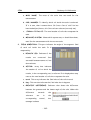
6.2.2. Rotation and level motor
A rotating motor can be assembled to the mole. It will be the responsible of rotating
the locomotive system: making the coils, inside the mole, turn in both directions. A
second motor that will level the set of coils to horizontal with respect to gravity once
the mole has been inserted into the magnet, is be also connected to the shaft. These
two motors are located outside the mole and the rotation is transferred to the coils
by modular shaft spacers. There are two sets of motors as the ones in the picture, one
in each of the sides of the shaft so that to allow measurements in the connection side
and in the back side.
Figure 6.5: Rotation and level motor at ICCA’s bench
- 59 -
CERN
Industry Coil Calibration
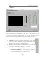
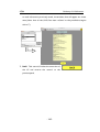
6.2.3. Inoxidable tube
53/50 mm inoxidable tube identical as the beam tubes in LHC magnets into which the
mole is inserted for making the measurements.
Figure 6.6: Inoxidable tube
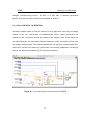
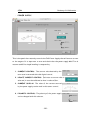
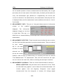
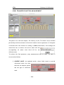
6.2.4. Power supply
The power supply gives power to the magnet so that to create the magnetic field. The
current to be set during the measurement can be selected previously as positive,
negative or both by software. Also, not only constant current can be set to the magnet
(remote or manually), but also cycles of current can be edited in order to make AC
measurements. For further information, see Appendix 5 FUG POWER SUPPLY NTN
300-60 DATASHEET.
6.2.5. NMR Teslameter
It is a device that measures in a very accurately way the field created into the
magnet. The field value, which is read by a probe fixed near the tube, from this
- 60 -
CERN
Industry Coil Calibration
Teslameter should be equal to the one reconstructed with data from the magnetic
measurement. For further information, see Appendix 3 NMR TESLAMETERS PT-2025
DATASHEET.
6.2.6. Position Control Unit
With the PCU connected to the mole’s encoder, the rotating and levelling motor are
totally controlled. For further information, see Appendix 4 PCU 2000 MAXON
MOTOR CONTROL DATASHEET.
6.2.7. Mole
A mole is a probe equipped with a 0.75 m long rotating coil and associated angular
encoder and motor. It slides into the 50 mm cold bore aperture and contains a light
source to transfer the transverse position of the coil rotation axis, and hence the
magnetic axis, to external fiducials via a telescope located at the magnet end,
however, the location of the beam axis will not be available for this system. Some of
the features that can be measured with the moles on the magnet are: integrated field
strength, field direction, distance between magnetic axis...
6.2.7.1. Coils
The search coils are made of a 20-wire flat cable wound onto a fibreglass reinforced
epoxy core. Each copper wire diameter measures 50 µm and the cable has a width of
1.3 mm. The windings have 400 turns, are 750 mm long and approximately 6.60 mm
wide for quadrupole coils and 11.30 mm wide for dipole coils between winding
barycentres. A tiny wiring board is inserted inside the coil core to interconnect each
individual wire of the multi-wire cable in series [22]. This set of rotating coils
(normally 3 or 5) provides voltage signals to be integrated depending on the angle of
rotation. With this array of voltage signals, the magnetic flux can be easily calculated.
- 61 -
CERN
Industry Coil Calibration
Figure 6.7: Cross section of the harmonic coils in the shaft
6.2.7.2. Incremental encoder
It is fixed on the coils rotation axis and determines their angular position. According
to specifications, the accuracy of the main field direction has to be better than 0.1
mrad that is why a 12 bits encoder has been selected.
6.2.7.3. Pneumatic brakes
Pneumatic brakes are set once the mole has been levelled to the corresponding value
and allows the coil spins in a secure way (the outer part of the mole does not move).
6.2.7.4. Electronic gravity sensor
The reference axis of the coils is adjusted by rotating the whole mole within ±300
µrad with a precision better than ±50 µrad. This precision is obtained using this
sensor.
- 62 -
CERN
Industry Coil Calibration
Figure 6.8: Mole and its cross section
- 63 -
CERN
Industry Coil Calibration
CHAPTER 7.
MAGNETIC MEASUREMENT PROCEDURE
7.1. PROCEDURE
The different steps to follow in a magnetic measurement are, in outline, the following
ones:
1. The field-measuring mole is inserted into the reference magnet.
2. The rotating motor moves looking for the zero position from which the measured
values will start to be acquired. Then, the motor turns exactly
2
rad in the other
3π
sense so that to reach a constant speed while crossing the zero position.
3. The level motor adjusts properly the level of the coils to horizontal (to 0 rad,
normally).
4. The brakes are set so that the coil can spin without that the locomotive rotates.
5. The power supply powers the dipole/quadrupole in order to create a magnetic field.
6. The coil spins two turns in one sense and two more in the other. Meanwhile, data
from the integrators are acquired thanks to a synchronization system.
7. More than one measurement can be done sequentially.
8. The field is measured by the NMR in every moment.
9. This sequence must be repeated by switching the coil wires manually since two
different sets of measurements per coil are needed in some of the cases (the so
called connection-side and back-side measurements).
10. Depending on the number of integrators available and the purpose of the
measurement, this procedure should be repeated for all the coils inside the mole.
11. For calibration purposes: MOLE PARAMETERS MUST BE UPDATED if it proceeds
after analyzing and/or comparing new RAW-DATA generated.
- 64 -
CERN
Industry Coil Calibration
It should be taken into account that there is often a configuration file (in a software
point of view) related to each measurement that stores all the necessary parameters
to carry out the process successfully (kind of current, number of measurements,
integrators’ gain...).
7.2. MEASUREMENTS
Each measurement consists in the reading of an absolute and a compensated signals as
delivered by rotating coils over a complete forward and backward rotation. The
angular encoder reads the coil angular position. [20]
It exists two different kinds of measurements: the absolute and the compensated
one. The absolute signal is obtained from the reading of a single coil (the so called
“measuring coil”, the one with the highest sensitivity to the main field component), and
is used for the determination or verification of the main field component. It is mainly
used for testing and checking purposes. The compensated signal (bucking signal), that
is to say the field harmonics, is obtained as a combination of the signals of different
coils, and is used for the determination of the field errors. The bucking allows
rejecting the main harmonic, so that a higher amplification of the voltage can be
applied to the field harmonics detection.
7.3. READING OF COIL VOLTAGE AND INTEGRATION
The two voltage signals (absolute and compensated) from each coil group are sent to
VME integrators that amplify the input voltage signal and convert it to a series of
variable frequency pulses. These are counted during the time interval determined by
two consecutive trigger pulses from the angular encoder. The counts obtained are thus
proportional to the integral of the voltage between two encoder trigger pulses. The
- 65 -
CERN
Industry Coil Calibration
result of each integration step, the flux increments, is available on the VME bus at
each angular interval. In addition, the integrator, via an internal time base, provides
the time interval between two subsequent trigger pulses from the encoder.
The flux increments are in units of “counts” from the VFC-counter unit. Counts are
proportional to the integrated voltage (Vs), and the constant of proportionality is the
product of the gains in the line of amplifiers and of the transfer function of the VFC.
For present integrators, different gains can be selected using jumpers. Typical values
used are 50 for the absolute signal and 500 for the bucking.
The time intervals are also in units of “counts” and are obtained from the internal
reference of 1 MHz in the counter. Time counts, proportional to the time interval
between two encoder pulses, are thus in units of (1/MHz), i.e. in practical terms in
units of µs.
The raw-data is considered to be the stored flux increments and the time intervals
for the forward and backward rotations, in a total of N angular points per rotation
(256 in this case) that will be later reconstructed and normalized in order to calculate
the field strength and its angle.
- 66 -
CERN
Industry Coil Calibration
CHAPTER 8.
HARDWARE SYNCHRONIZATION
As seen in previous chapters, there are several types of instrument that composes the
system. Some of them, like integrators and ADC cards, use a fast VME bus to
communicate with the Sun workstation; others, like motors and power supply, use slow
RS-232 serial line or GPIB bus. All the instruments must cooperate and be
synchronized to achieve good measurements.
Instrument synchronization is very important because affects the measurement
precision. The RCM software must synchronize together the angular motor, the
integrator and the magnet power supply during a measurement if it is done in AC
(current cycles are set). In other versions of the magnetic measurement program, the
axial motor must also be synchronous with all the measurement system but the
software control for calibration is simplified since the mole stays in the same position
during the whole measurements. Also to remark that only DC measurements will be
performed for this purpose.
8.1. ENCODER, INTEGRATORS AND ROTATING MOTOR INTERACTION
The 12 bits angular encoder synchronizes the angular motor with the integrators by
means of hardware triggers. The encoder is able to send to the integrator two types
of trigger:
1. The sample trigger: used to communicate to the integrator to read a new voltage
value from the coil.
- 67 -
CERN
Industry Coil Calibration
2. The zero trigger: used to communicate to the integrator that the coil is in the
zero degree position and the data acquisition must begin. The integrator will
receive the zero trigger each time that the coil execute a complete rotation.
More integrators can be used, but just one must be linked to the angular encoder. The
first integrator will propagate the trigger to the next one. The next figure shows how
the motor and integrators work together during a measurement:
Motor rotation speed
B
C
A
Angular position
The integrator receives a zero trigger from the encoder.
The integrator receives a sample trigger from the encoder.
Figure 8.1: Synchronization between the encoder and the rotation motor
A: the angular motor accelerates up to the speed selected by the user. The
acceleration is constant and also the speed must be constant during the measurement.
B: the angular encoder sends a zero trigger to the integrator when the angular motor
(and so the coil) reaches the start position for the data acquisition. 256 values are
acquired for each coil turn. To spread the data evenly the angular encoder sends a
sample trigger to the integrator (and the integrator samples a new data) every 1.4
degrees approximately.
sample rate =
360deg
= 1.40625
256
(7.1)
- 68 -
CERN
Industry Coil Calibration
After the coil executes a complete rotation, the integrator receives another zero
trigger because the coil is again in the start position and the data acquisition stops.
C: the angular motor is decelerated until it stops. This is the description of the first
part of the measurement. In the second part the instruments execute the same task
but the angular motor rotates in the opposite way. After the measurement, the motor
is in the start position again.
8.2. POWER SUPPLY SYNCHRONIZATION
With the Real Clock Measurement software, the user can define a set of
measurements to be executed at different currents. The magnet power supply is an
independent device and so it must be synchronized with the rest of the system by the
software.
The CPU pools the magnet power constantly. When the current reaches a point where
a measurement was defined, the measurement is executed. The SUN cannot pools the
magnet power supply in real time because it is usually linked by a low-speed serial line
(RS-232, GPIB or serial-GPIB) and so the measurements are executed with a small
delay. However, an ADC card could be used in some racks, when the reading of the
current is critical.
Current
∆I
Time
∆t
∆t
Where measurement is executed.
Where measurement is defined.
Figure 8.2: Delay while reading current by a low serial line
- 69 -
CERN
Industry Coil Calibration
The delay is never bigger than one second, anyway; hence, this does not affect the
measurement executed at constant current. It can be observed that during the
measurement with variable current the measurement is executed at a different
current with respect to the defined one. The measurements at variable current are
usually executed with slow ramp rate and so a delay is not a problem. The
measurements will be valid anyway because the current is read directly from the
magnet power supply before and after the measurement.
8.3. ROTATING MOTOR SYNCHRONIZATION
The user can select the rotation speed of the rotation motor but the measurements
must be executed at constant velocity. The angular encoder sends the zero trigger to
the integrators when the start coil position is reached but if the user selects another
rotation speed of the motor, then the next measurement will be not correct because
the integrator will receive the zero trigger in a wrong position:
Rotation speed
V2
Vref
V1
Angular
position
The integrator receives the zero trigger
from the encoder .
Figure 8.3: Zero trigger position when the rotation speed changes.
If a set of measurements have been executed with rotation speed Vref and the
rotation speed is decreased, (for instance to V1) the integrator will receive the zero
- 70 -
CERN
Industry Coil Calibration
trigger from the angular encoder in late and the data acquisition will start in late (the
acceleration is constant).
If a set of measurement have been executed with rotation speed Vref and the rotation
speed is increased (to V2), the integrator will receive the zero trigger from the
encoder too early and the measurement will begin at a non constant rotation speed and
so the measurement will be non valid.
The RCM software calibrates automatically the angular motor. Each time the user
changes the rotation motor speed, the software will search the new start position to
execute the next set of measurements with constant rotation speed. The software
find the new motor start position by executing a dummy measurement.
To prove that the dummy measurement is enough to find the motor start position let’s
see what happens when the motor speed is increased and decreased.
8.3.1. Motor speed decrement
Rotation speed
Vref
V1
P
The integrator receives a zero trigger from the encoder.
The integrator receives a sample trigger from the encoder.
Figure 8.4: Motor speed decrement
- 71 -
CERN
Industry Coil Calibration
During the forward motor rotation, the integrator receives the zero trigger from the
encoder in late. The acquisition starts in late too, but all the 256 voltage values are
read and the motor is decelerated. During the backward motor rotation, the
integrator will receive the start trigger as soon as the motor reach the constant
rotation speed because the acceleration and the deceleration speeds are the same.
After the measurement the motor will be in a good position (P) for the next
measurement. This case is not problematic; the data is valid because values have been
read while coils were rotating at a constant speed.
8.3.2. Motor speed increment
Rotation speed
V2
Vref
P
The integrator receives a zero trigger from the encoder.
The integrator receives a sample trigger from the encoder.
Figure 8.5: Motor speed increment
During the forward motor rotation, the integrator will receive the zero trigger from
the angular encoder when the motor is still accelerating. The data acquisition will start
too early but after one turn the motor is decelerated until it stops. During the
backward motor rotation, the motor will stop in a good position for the next
- 72 -
CERN
Industry Coil Calibration
measurements. Unlike the other case, the data achieved is not valid since the values
are not evenly read because of the rotation speed was not constant.
8.4. NMR TESLAMETER
A Teslameter or magnetometer is a useful electronic device used for any application
where rapid, fully automatic and very accurate measurements of magnetic fields are
of primary importance. It is commonly used in accelerator beam handling since they
are easy to use and to control remotely (by serial or GPIB bus) as well as the accuracy
of the field value reading is quite good.
8.4.1. Synchronization
Fortunately, it must not be synchronized with any other device of the system since
the magnetic field remains always constant inside the magnet. This value, then, must
be read at any time to be used afterwards for the analysis.
8.4.2. Theory of operation
Nuclear magnetic resonance is based on a spin-echo nuclear magnetic resonance
effect. The spin-echo frequency f nmr and the magnetic field B are connected by gyro
magnetic ratio g:
B=
fnmr
.
g
(7.2)
The physical constant g for different kinds of nuclei is precisely known, so the field
strength
measurement
accuracy
is
determined
by
the
spin-echo
frequency
measurement accuracy. Nuclei of the substance in the probe are excited by two short
pulses of RF field with the frequency close to the NMR frequency, thus causing the
spin-echo signal. Each probe is connected to NMR exciting and receiving electronics by
- 73 -
CERN
Industry Coil Calibration
a multiplexer. A frequency synthesizer is used for both exciting and receiving the
spin-echo signal. A measuring cycle is organized by a control module.
There are some limiting factors, which decrease the measurement accuracy. The most
significant of them are the signal-to-noise ratio and finite duration of the spin-echo
signal defined by field in-homogeneity in the probe volume. Low-noise preamplifiers
are placed near every NMR probe to decrease losses of the spin-echo signal in RF
cable between the probe and the Magnetometer. The amplified signal is shifted to a
low frequency region by multiplying it by two orthogonal signals of precisely known
reference frequency close to FNMR. After narrow band low-pass filtering the output
signals are digitized by ADC. In computer they are multiplied by Gaussian shaped pulse
which width is equal to the spin-echo signal to maximize the signal-to-noise ratio. The
carrier frequency is determined according to the spectrum obtained by Fast Fourier
Transform. The data measured can be accumulated to give further increase in the
relative accuracy of the magnetic fields measurements. [23]
8.5 DATA ACQUISITION
The SUN workstation can read integrators by a VME bus with enough bandwidth to
allow real time data acquisition. This data acquisition from the integrators is the most
critical part of the system since they do not send any trigger to the SUN workstation
directly when the data are ready. The VME CPU card receives the encoder trigger as
well as the integrators; that way, it is known when the measurement is finished and
the integrator cards are ready to be read by the CPU. Meanwhile, these values are
read by the SUN workstation via the VME bus.
The needed acquisition rate depends on the motor rotation speed. The motor speed is
not usually bigger than 1 rotation per second and so the maximum rate is:
- 74 -
CERN
Industry Coil Calibration
256 values 1 turn
values
⋅
= 256
turn
sec
sec
(7.3)
That is a value every 3.9 msec approximately, the data acquisition rate required to
read a single integrator. In other applications, during multi coil measurements, many
integrators must be read at the same time; then, the acquisition rate become
proportional to the number of integrators.
- 75 -
CERN
Industry Coil Calibration
CHAPTER 9.
PERIODIC MOLE CALIBRATIONS AND PROCEDURE
9.1. WHAT TO CALIBRATE
The parameters that define a mole are the following ones:
1. Coil surfaces.
(m2)
2. Parallelism between coils.
(mrad)
3. Radii of coil rotation.
(mm)
4. Distance difference in coils plane.
(mm)
5. Perpendicular distance difference to coils plane.
(mm)
6. Level zero error.
(mrad)
7. Level transfer function.
(mrad/V)
The concrete aim of the calibration software developed (ICCA) is to follow an
evolution of some of these important parameters of the moles. Most of these are
related to the geometry of the coils inside the mole (coil surfaces, radii of coil
rotation) and their situation and equivalence with respect to the others (parallelism,
distance difference between their planes). That means that with a good calibration
and assuring, periodically, that these parameters are well calculated, the geometric
coefficients will contribute with real measuring conditions; hence the harmonic
coefficients will reflect reliable field features that will be easily differentiable from
offsets or noise.
If this is feasible, it will be possible to check, and correct in some occasions,
deviations in the mole’s structure, from initial features through time, due to its
constant handling, variations of temperature, possible mechanical or electrical
- 76 -
CERN
Industry Coil Calibration
damages, manufacturing errors... So that it is like this, a detailed operational
specification for the mole’s calibration is available in Annex 1.
9.2. COIL SURFACES CALIBRATION
Achieving reliable values of the coil surfaces is very important since they are deeply
related to the coil coefficients. As demonstrated earlier, these coefficients are
needed in order to reconstruct the exact value of the magnetic flux. In case these are
not well calibrated, the final value achieved would not reflex the amount of flux that
the magnet really creates. The relation between the coil surfaces, considering perfect
radial coils, and the coil sensitivity coefficients can be easily explained by recovering
some of the equations presented (4.17) in previous chapters:
Figure 9.1: Coil coefficients calculation with LabVIEW
- 77 -
CERN
Industry Coil Calibration
n
n

Nt L
N t L n n Nt L
S  
S  
Nt L 
n
n
kn =
cn =
(z 2 − z1 )= n (z 0 + ∆z 0 ) − (z 0 − ∆z0 ) = n  z0 + 2N L  −  z 0 − 2N L  
n
n
t
t


(
)
χ n = (z2n − z1n )
(9.1)
z n2 = (z0 + ∆z0 ) ;z n1 = (z0 − ∆z0 )
n
∆z0 =
n
S
2N t L
To calculate the surface value of one coil inside the mole, after connecting the
absolute integrator to it, a standard magnetic measurement (see next section for
further details) must be performed. As the field value from the Teslameter will be
extracted and the magnetic flux can be reconstructed from the measurement rawdata obtained, the calculation of the new data can be easily calculated as:
S c REAL =
φ max
φ
= max
B cos(α )
B
(9.2)
The REAL coil surface value is given when the angle between the surface vector and
the magnetic field vector is zero. (see figure 4.6). This value will be compared to the
some time ago calculated one. If the difference between both exceeds the acceptable
limits, 300 µm2, the old value can be overwritten by the new one, in all the
corresponding files, after saving it in a historic file. In case that more than one
measurement is performed sequentially, the average of the resulting surfaces will be
saved.
9.3. PARALLELISM BETWEEN COILS
The aim of this calibration is to check that all the coils inside the mole are coplanar,
that is to say, if there are not big differences between the angle created by the
magnetic field vector and the axis of the coils. Unlike the coil surfaces, this
parameter cannot be corrected but only checked. The procedure followed in the
- 78 -
CERN
Industry Coil Calibration
program is the next one: It must be performed as many sets of measurements as
number of coils inside the mole in order to calculate a field angle value from each coil
since there is only one integrator for absolute measurements per coil (the ideal would
be to profit each set of measurements for the calculation of all the angles of the
coils). For all these measurements, the levelling value of the coils is expected to be
the same (always to 0 mrad, for instance, as it is done in the program) so that to
compare the reconstruction of all the field angles to a same reference tilt sensor
value. These are stored while they are obtained and later they can be compared. If
the greatest angle difference between two of the coils exceeds the maximum
tolerance allowed (selected by the user) may this mole has got a mechanical default,
coils are not in the same plane, and hence it is not an appropriate tool to use as a
probe. The program developed will warn about this since it cannot modify physically
the orientation of the coils.
In this case, the accuracy and reproducibility of the levelling system and its software
is very important since a deviation in the adjustment of the reference axis bigger than
50 µrad may imply the acceptance of bad results due to the difference between angle
references for each coil.
MOLE LEVELLED TO ß mrad
QuickTime™ and a
Graphics decompressor
are needed to see this picture.
ß
Figure 9.2: Are all the calculated field angles equal to the reference β mrad?
- 79 -
CERN
Industry Coil Calibration
9.4. LEVEL TRANSFER FUNCTION
The level transfer function is a parameter that allows knowing whether the tilt sensor
attached inside the mole works in a proper way and whether it is linear in the working
region or not (between ±2 mrad). This parameter is a relation between the
reconstructed field value (in mrad) achieved from the measurements of each coil and
the reading of the levelling sensor (in V). If the results demonstrate a good
correlation between those variables, the result should be a straight line passing
through three coordinates (or even more in the mentioned range, although the
software is only presented for three different ones) with a slope value approximately
equal to 1.454.
angle from the measurement(mrad)
gravity sensor value(V)
0.5 deg πrad 1000mrad
⋅
⋅
= 1.4544 mrad V
6V
180 deg
1rad
LTF =
(9.3)
The procedure to reach the final level transfer function is simple since it has few
variations with respect to the acquisition of previous parameters for calibration but
with the difference that the number of measurements increase. Up to a total of 6
different sets of valid measurements (each set can be composed of n measurements)
per coil must be accomplished: there are three different levelling values (0 mrad, +2
mrad, -2 mrad) and two measurements to be carried out per each one (one from a
connection side and another one from the back side). After calculating the average of
all of them, the desired value is achieved. If there would be a considerable difference
from the expected value, that would probably mean that there is a problem with the
gravity sensor or that the physical position of the coil is not correct.
- 80 -
CERN
Industry Coil Calibration
9.5. LEVEL ZERO ERROR
Profiting the previous procedure, the level zero error can be corrected, too. The field
directions in connection and in back side should be equal independently of the levelling
value (tilt sensor reading). If they are different, the level zero error is corrected
with the average of them. There are two interesting angles to take into account, the
field angle and the mole angle:
θ conn − θ back
2
θ conn + θ back
=
2
θ field =
θ mole
(9.4)
Figure 9.3: Field and mole angle’s calculation in LabVIEW
The field angle must be next to zero since the connection-side and the back side
angles from the measurement are expected to be equal (as long as the calibration
bench is stable and it does not move) whereas the mole angle must be nearly equal to
the one read from the gravity sensor.
- 81 -
CERN
Industry Coil Calibration
CHAPTER 10.
ICCA SOFTWARE
ICCA has been totally developed in LabVIEW 5.1. There are several reasons for having
used LabVIEW but the most important one is that a program destined for magnetic
measurements (MMP) had already been designed in this language. Many versions of
MMP have been developed by the AB/CO/IS/LS subsection since requests for
different systems and with different analysis and procedure applications increase.
One of the versions used at QIMM systems has been recovered, modified and adapted
in order to apply the calibration requirements.
ICCA is formed by more than 400 subVI and more than 20 different panels can appear
while dealing with the program. Since LabVIEW’s code cannot be printed as easily as it
could be done with another high level programming language (C, Java…), only a few
programming examples, structures and techniques will be shown (but no utility
matters; for this topic, see the user’s manual in Annex 2.). Moreover, there are two
attached text files where all the changes done to ICCA project (ICCAchange.txt)
were updated regularly and the different releases generated by those updates:
addition of new important VI, changes in structures, code compacting into VI, addition
of controls or indicators… It has been a useful tool to refresh and recover changes
done some time ago from previous versions.
10.1. LABVIEW
LabVIEW programs are called virtual instruments (VI) and they are composed of
three main parts: a front panel, a block diagram and a icon-connector.
- 82 -
CERN
Industry Coil Calibration
The front panel allows the user to set the input values of the program and to view the
outputs from the VI block diagram. Because the front panel is analogous to a front
panel of a real instrument, the inputs are called controls and the outputs are called
indicators. There are a variety of controls and indicators hence the programmer can
create the front panel easily identifiable and understandable.
Each front panel has an accompanying block, which is the VI program. The language
used to build this diagram is graphical and it is called language G. The block diagram
replaces the normal source code of other languages and its components represent
program nodes; for example: for loops, case structures, arithmetic functions… The
components are wired together to define the flow of data within the block diagram.
The part of the icon-connector is used to turn a VI into an object (subVI) that can be
used as a subroutine in the block diagrams of other VI. The icon graphically
represents the VI in the block diagram of other VI. The connector terminals
determine where the inputs and outputs must be wired on the icon. The terminals are
analogous to subroutine parameters. They correspond to the controls and indicators on
the VI front panel.
LabVIEW sets a special hierarchy at the VI components. After creating a VI it can be
used as a subVI in the block diagram of a higher-level VI. There is no limit on the
number of layers in the hierarchy.
10.2. PROGRAMMING STRUCTURES
10.2.1. Index VI’s structure
The main menu’s diagram is composed by a 14 cases structure, located into a main loop,
through which the flow of the program can be passed to the NMR device control, to
- 83 -
CERN
Industry Coil Calibration
the power supply control, to the panel for the creation of configuration files, to the
execution of measurements, to different panels to recover data…
The circled code is a common structure used when there are a lot of controls among
which the user can choose. Depending on the boolean output index set to true in the
array (button pressed or action taken by the user), a concrete code will be executed
from the case structure. In the case shown below, when no buttons are selected, and
depending on other choices from the front panel, some indicators are refreshed or
updated by information extracted from some files.
Figure 10.1: Frame “0” in Index VI’s diagram block
10.2.2. Area VI’s structure
This is a part of the code inside the initialization frame of the Area VI’s diagram. This
code, inside a for loop, is reached either when a set of measurements has immediately
- 84 -
CERN
Industry Coil Calibration
finished or because data from last measurements (from the last *.CFG file) want to be
analyzed for recalculating the coil area. In any case, information from measurements
are recovered from *.RF files (code inside a black circle).
After recovering and detaching data of every measurement, through some analyzing
stages (frame 0), and after achieving a field locked value from the Teslameter (frame
1, inside a green circle) the new surface value, the harmonic coefficient Cn, the field
angle, the temperature of the measurement, the maximum value of the absolute flux
and the NMR value of each measurement referred to the coil selected will be
displayed (frame 1 and frame 2) and ready to be saved if proceeds.
Figure 10.2: A part of the initialization frame in Area VI’s diagram block
- 85 -
CERN
Industry Coil Calibration
10.2.3. Parallelism VI’s structure
Figure 10.3: Checking the parallelism between coils in Parallelism VI
From the VI destined to the Parallelism calibration, I have found interesting to show
how the names of the files are structured and how information from them is
extracted in order to display it in the indicators.
When the user selects a file from the “set of coils“ list, its name is detached through
some filters so that to show the correct information about it: the name of the mole,
the position of the coil (0 in this case since all them are selected), number of coils,
- 86 -
CERN
Industry Coil Calibration
kind of measurement… and also to look for the path where this file remains. The
corresponding extension is added to the name of file, then, and it is read (frame 0). In
the following frame, the data loaded is treated and depending on the results, a
warning message is shown.
10.2.4. LevelTRansFunction2 VI’s structure
Figure 10.4: Saving data to a *.LOG file in LevelTRansFunction2 VI
- 87 -
CERN
Industry Coil Calibration
This is to show how data is saved to a log file. The name of the file to be saved is
formed from the different indicators that contribute with information about the mole
and coils. After confirming the storage operation, the results from a table are divided
into arrays (thanks to a for structure) and they are saved into a file.
10.2.5. RC_MagnetInformationsPanel VI’s structure
Figure 10.5: ‘Call?’ frame inside Rc_MagnetInformationsPanel VI
This is the structure used in the VI where the configuration file is set (visible for the
user) or the measurement procedure starts (not visible for the user). A software
button has been added, ‘Call?’, so that to take the control of the program to an
- 88 -
CERN
Industry Coil Calibration
invisible state for the user but where the measurements take place automatically and
all the information is correctly passed.
In the picture above, information from a file is recovered and displayed in some
indicators and some global variables are initialized to start the measurement.
10.2.6. ICCA_LevelMotor VI’s structure
Figure 10.6: Part of the block diagram for the levelling motor control
- 89 -
CERN
Industry Coil Calibration
This is the most interesting part of the VI that controls the levelling motor. The
structure is the following: The levelling motor turns the coils towards the selected
value (0, +2 or –2 mrad) with a concrete speed, acceleration, and angle value depending
on the absolute difference to the goal (red square). After being moved, the angle is
read from the ADC card (tilt sensor) and it is checked if it is into acceptable limits. If
it is not like this, the motor moves again depending on the new difference to the goal.
Meanwhile, the data is updated in the front panel (blue square). Once the mole level is
between acceptable limits, the brakes are set.
10.2.7. RC_MakeMeasureSaclay VI’s structure
Figure 10.7: Data acquisition from integrators.
This is the most critical part of the whole program. It is when the SUN workstation
polls the integrators in order to read their values in Real Time. It is into the circled
VI where this is done.
- 90 -
CERN
Industry Coil Calibration
10.2.8. RC_DisplayMeasurePanel VI’s structure
Figure 10.8: Part of the code of Harmonics.vi
To conclude, here it is a VI destined for analysis. This block diagrams is the result of
the standard procedure to achieve normalized harmonics, explained in chapter 5
“Standard Analysis of Raw Data”.
- 91 -
CERN
Industry Coil Calibration
10.3 HISTORY OF CHANGES. ICCAchange.txt
26-6-2001 Adriaan
Avec 3 s. avant le premier point, tous les points sont mesurer correctement.
Avec 2 s. avant le premier point, le deuxieme point est blanc (saute).
Avec 4 s. avant le premier point, le premier point est blanc (saute).
Q1: quel temps est necessaire avant un point (ou le premier point) pour qu'il
prend la polaritee demandee en compte?
Q2: Ou est defini ce temps?
Peut etre il faut toujours rajouter ce temps avant chaque serie de mesures.
Le PS_control.llb/getPolarity.vi ne pilote pas le Serial-GPIB/Bus-GPIB entree.
On appelle directement le GPIB_Write_(Bus_or_Port).vi tandit que dans
InitPS,
ChangeCurrent
et
ChangePolarity
on
utilise
le
PS_control.llb/writeGPIB.vi qui tiens compte du choix d'interface.
Dans writeGPIB.vi j'ai change le Serial-GPIB/Bus-GPIB de control (initialement
prevu) dans un indicateur.
J'ai rajoute le test sur le choix d'interface dans getPolarity.vi.
Dans user.lib/GPIB_Read_(Bus_or_Port).vi le byte count dans la lecture n'a pas
ete fixe. J'ai rajouter une conversion string-nombre pour convertir le
Buffer_Size dans byte count. Ceci est a controler dans les autres librairies
avec le GPIB-Serial.
Meme avec ces corrections le getPolarity.vi ne marche pas.
La commande est N2, suivi d'un x, mais la reponse est toujours "courant
positif". Le code retourne est 1010000, et on teste le 5eme bit (de gauche) 0
ou 1. On compte 0 le premier. Est-ce qu'il y a un probleme avec cette alim?
La commande N0 donne le voltage (toujours +)
La commande N1 donne le courant (toujours +)
La commande N2 donne le code 1010000
La commande N3 donne +60
La commande N4 donne +20
- 92 -
CERN
Industry Coil Calibration
La commande N5 donne IB40 V1.30
La commande N6 donne 10807012
In changePolarity.vi dans la sequence 5 il y a un test en boucle si le courant est
dans la limite de 0.01 de la valeur demande. Mais il n'y a pas de time-out, ni
message d'erreur si cette condition ne peut pas etre remplis. Une erreur sur
l'ADC ou l'alim peut faire tourner cette boucle pour toujours.
Il faut changer ! (J'ai rajoute un graph pour voir la montee du courant).
On a supprime le test sur getPolarite dans RC_PowerSupplyControlSaclay.vi
mais il est necessaire parce que si on appelle dans chaque verification le
changePolarity le courant est mis a zero avant de le remettre sur la bonne
valeur. Il faut ou obtenir la polarite du ADC (si l'alim ne la donne pas) ou le
faire a l'interieur de changePolarity.
27-6-2001
In initPS.vi seq 0 we should first test which interface (Serial/GPIB) before
initialising any port.
On the front panel of changePolarity.vi I have added the GPIB address control.
This should become an input and be driven from the callers OR we should use
the global variable defining the power supply GPIB address.
29-6-2001
In changePolarity.vi we have added a global RC_PS_Polarity.glb this memorises
which polarity we set
In getPolarity.vi we have added a switch to take the polarity from this global or
from the power supply. Default is from the global.
We have put back the test on getPolarite dans RC_PowerSupplyControlSaclay.vi
which is needed because the current is being put to zero before putting it to
the required value.
Vi's changed to give more info through indicators:
Motor one acc.vi
LevelMotorControl.vi
LevelMotor.vi
motorAdjustmentPanelNewModified.vi
- 93 -
CERN
Industry Coil Calibration
16-11-2001
In the changePolarity.vi frame 5 the delay in the for loop was set to 200 ms.
This is too short to reach stable current for the measurement. I have
increased it to 500 ms. But I had to increase the number of iterations (N=5 to
12) to get a stable current. This is using the supply Fug NTN1400 M-70. I have
made the N loops a control so it can be adjusted if necessary without stopping
the program.
The getPolarity has been changed to make it execute faster when we get
polarity from memory. A case just for that. Previously the supply was
interrogated but then the answer ignored when the switch was in "from
memory". This is time consuming (6 to 7 seconds, the way it was done).
*********************************************************************
15-2-2002 Adriaan
On sunmms19 the serial extension software is not installed.
The admintasks don't set the priviliges correctly for this machine (paths
to be changed).
The MMP software has been copied from sunmms1.
The nonvxi table has been copied from sunmms1.
The Init4SUN.vi has been copied from sunmms18.
We could include some improvements here that we have made on the sunmms18.
11-3-2002 Adriaan
On sunmms21 a init error on serial port occurred (error 37) because the two
ports on the machine were not set to read/write for all users.
The admintasks don't set the priviliges correctly. Paths should be changed for
the two machine ports. They are on /devices/pci@1f,0/isa@7/
I issued the command
chmod 666 *,cu
in the above mentioned directory and all works fine. Magnus should have a look
at the admintasks script.
- 94 -
CERN
Industry Coil Calibration
25-06-02 Hubert
Load_HarmMaxMin.vi created & saved in Disp.llb. Used to load the "HarmMaxMin.cfg" file (from the config folder), through the "RC_ZoomMP.vi", which
is used to display the harmonics of the 5 positions.
28-06-02 Peter
new_changePolarity.vi : now used in place of "change_Polarity.vi":
frame 0 : call to "new_changeCurrent.vi:
frame 3 : command "x" send to execute the polarity change
frame 4 : waining time = 1sec
frame 5 : call to "new_changeCurrent.vi:
new_changeCurrent.vi : now used in place of "changeCurrent.vi":
loop 0 : command "F1" to enable output
loop 1 : command "u..."
loop 2 : command "i..."
loop 3 : command "x" to execute the previous commands
02/07/02 Hubert
Rc_NewFeed-down Corr_spec.vi : correction du signe pilote par "Magnet order"
en case = TRUE. Maintenant on * toujours par +1. A verifier par des analyse de
VR.
24 07 02 Hubert
Modification in "motorAdjustmentPanelNewModified.vi" to manage the both 3b
& 6b brakes.
01/08/02 Hubert
RC_HarmonicPart3.vi : CenterLocalization_new.vi was present but
connected. Now has been connected & Center.._1.vi has been removed.
- 95 -
not
CERN
Industry Coil Calibration
27-09-02
New_changePolarity.vi :"N loop" has been set by default to 5 (before was 12).
04-10-02 Hubert & Peter
Function to put the rotating coil motor in the start position has been removed.
"Test Coil Start Position.vi" created to put the coil motor in the start pos, and
called from "RC_SetupPanelm.vi".
RC_Brake_3b.vi : modified to set or reset this brake without modifing the
setting of the others.
RC_Brake_6b.vi : the same.
RC_RemoveAllBrakes.vi : created to remove all the brakes, and called as
replacement of the call to Brake_3b or Brake_6b.
motorAdjustementPanelNewModified.vi : sequence added on the left:
frame 0 = "check limit"
frame 1 = remove brake-3b if out of limit
Main case = false modified: frame 1 of the sequence, while loop on the right:
To compare the ADC reading of the tilt sensor, with the 10 mrad & 0.5 mrad
values, the output of the ADC is * 1000 and / 600.
Then in the case:
0 = this value is put in "coil angel"
1 = this value is put in "coil angel"
2 = this value is * 1000, then put in "coil angel"
Motor Control.vi :Acc set to 15 (was 100).
Init Motor.vi : added in "make measure.vi" sequence "init"
Mspecpanel.vi : just before the call to "level.vi" (measurement case) brake 3b
set to ON.
21-05-2003 Hubert
- 96 -
CERN
Industry Coil Calibration
The RC_MDISP.llb of the MMP_560 has been copyed in the MMP_562
application. This will fit the request of Vittorio (19-05-2003), to have the
MMP_560 analysis + all the modifications done for the brakes control of the
MMP_562.
This modification generate the MMP_563 release.
26-05-03 Hubert
motorAdjustmentPanelNewModified.vi:
FALSE, seq 2 (0-2), FALSE, WHILE loop:absolute value function before the
"coil angel" local variable has been removed to have an indication via the arrow
related to the sign of the angle value.
FALSE, seq 1 (0-2), WHILE loop on the right: a selector has been added to put
the normal value or the negated one according to the sign of the value of the
gravity sensor (via AD), on the "coil angel" local variable selected.
++++++++++++++++++++++++++++++++++++++++++++++++++++++++++++++++
MMP MODIFICATIONS FOR ICCA PROJECT
09-07-03 Ricardo
RC_MagnetInformationsPanel.vi
In the front panel, a new control has been added: "measurement system" with
which we select the kind of system the calibration is going to be performed.
Depending on the selection, the communication with the Teslameter is one or
other so, before accessing this vi, a warning message is showed (so that to be
sure that a different choice than "none" is selected).
NMR_teslameter.vi has been completely substituted by NMR_Panel.vi in case
called "NMR PANEL" and in RC_DisplayMeasurePanel.vi. The new release has
got an input: Communications parameters and two outputs: list of values and
display. Moreover, a new global variable to save the locked value has been
created. This global value is essential to calculate the correct coil area in its
calibration.
- 97 -
CERN
Industry Coil Calibration
With this new release it is now allowed to communicate to the Teslameter by
three different vias: GPIB, Serial Port or Serial-GPIB (although this last is not
still properly functioning) depending on the type of measurement it is going to
be done (QIMM or DIMM). Of course, the NMR_READ.vi and the
NMR_WRITE.vi have also been changed. So, RC_CalibMagnet.vi has also been
modified because of this.
"Measurement Type" control has been added one more item. A default, nonused one (Index=2), so that to force users to choose an correct option each
time a measurement is done or a config file is saved.
"Magnet type" control has been reduced in 4 choices (to maintain the
correspondence to the global variable Measurement Data): Dipole, quadripole,
sextupole and none (this last time inserted for the same reason than the
previous parameter).
Case MEASUREMENT:
Some cases have been put in just one (case 3) because all them are deeply
related --> messages to the user informing that something is not properly set.
It has also been added three new sub cases (into case 3) in which a message is
shown in case the measurement system, the measure type or the magnet type
are not selected. If some of the warning messages are shown, the measurement
execution is not going to be achieved. That way it is assured that main settings
are correctly selected.
Case Magnet Power Supply:
powerSupplyPanel.vi has been modified by connecting a string control,
GPIB_address, to all the subvi that need it. GPIB_Write has been modified in
the same way.
15-07-03 Ricardo
RC_MagnetInformationPanel.vi
-In the front panel, a new control has been added. It is only visible when the
MMP application is selected from the ICCA Main Front Panel (Index.vi). It is
- 98 -
CERN
Industry Coil Calibration
used for creating a Configuration File (*.cfg) where all the information needed
concernig to the coil parameters is stored. It must be assured that all the
parameters saved are correct and the file names refers to a correct file
before creating it:
CASE "Measurement":
Some changes has been inserted. Measure type and Magnet type variables are
located outside the sequence structure to reduce the number of local
variables.
FRAME 0: Remains the same.
FRAME 1: Checks if measurement parameters are properly selected and
the user has not taken the default values. Warnings are shown if proceeds.
Unless all the parameters are selected properly, the rest of he code is not
going to be executed. Before the modification, all the global variables were
updated and then they were checked. That way, unnecessary operations are not
taking place.
FRAME 2: Checks if all coils are full configured if no error in frame 1.
Otherwise integrators are reset (old 4th frame).
FRAME 3: If no problems in the previous frames, parameters common to
all coils are saved in global variables (old 2nd frame).
FRAME 4: If no problems in the previous frames, rotation speed,
motorpositionOK?, UsedIntAddressList and UsedIntGainList are updated. (old
frame 1 with the peculiarity of adding a none Measure Type case -just to
respect the number of choices of the variable but unnecessary because it has
been checked earlier and there is no way to entry in this part of code-)
FRAME 5: Remains the same.
FRAME 6: Remains the same if no errors earlier.
23-07-03 Ricardo
RC_MagnetInformationPanel.vi
CASE "Create Config File":
FRAME 0: Check that the CoilSetName refers to a correct, existing file.
FRAME 1: Check that measure parameters are properly selected (no
default vales).
- 99 -
CERN
Industry Coil Calibration
FRAME 2: First part of the file is saved. RC_MeasureSpecSaclay.vi is
called with input "caller"=2. Value that drives the .vi to a suitable ICCA panel
(to save the second part of the config file).
CASE: "CALL?":
Also, another software control (never visible for users) has been added. It is
called "call?". This is to entry in the MMP application in a remote mode, that
does not allow any interaction with the user. The measurement is anyway
achieved.
The config file selected by the user is loaded only if it really exists:
FRAME 0: Magnet data and encoder data is saved in global variables.
FRAME 1: Coil data is saved in a global variable by loading by means of
the coil_set_name parameter.
FRAME 2: Integrator addresses are saved in global variables depending
on measure type.
FRAME 3: Here it is called the RC_MeasureSpecPanelSaclay.vi where the
levelling takes place.
FRAME 4: After the levelling and the measurement itself,
RC_DisplayMeasurePanel.vi is called.
The format of *.CFG files are the
following:
"S"@"mole_name"-COIL"X".cfg
"S"=D if DIMM S=Q if QIMM;
"X"=number of the coil to be measured: 1,2,3,4 or 5;
04-08-03 Ricardo
RC_MeasureSpecPanelSaclay.vi
-As it has been done in RC_MagnetInformationPanel.vi, a control related to the
creation of the configuration file has been inserted. It is not visible unless the
input "caller" is equal to 2, that means, after saving the first block of the
configuration file.
"INITIALIZATIONS":
CreateConfigFile's attribute node set to False so that no to be seen. Just set
to true in the concret place.
- 100 -
CERN
Industry Coil Calibration
‘ICCA_LEVEL?’ --> global variable always set to False in order to not modify the
normal execution of the vi. It is only set to True when, in the ICCA program, it
is wanted to level to a different angle than 0 mrad. Then, as it expected, the
levelling of the coil is not taking place reached this point because the selected
levelling of the coil is already done (from the ICCA program) .
NEW frame created: Caller=2 -->
FRAME 2: Only the interesting parameters for the measurement (to be
saved in the 2nd part of the file) are visible. The rest
is set to non-visible.
NO BUTTONS:
Global variable CALL?.
FALSE: Drives to the normal execution as it has been up to the moment.
TRUE: Means we are performing the measurement in remote mode.
FRAME 0: SpecP parameters are saved in global variables. And
Cycle Data if proceeds.
FRAME 1: RC_MakeMeasureSaclay.vi is called. Measure File Name
is saved in a global variable, too.
FRAME 2: Since the measurement is finished, the VI is forced to
be closed.
"Create_Conf_file":
This point of the project is reached when it is wanted to save the remaining
parameters (2nd block) for the configuration file.
FRAME 0: If Current Cycle is selected, it is assured that the cycle name
really exists and corresponds to a cycle file.
FRAME 1: Current type, cycle name, current mode and Number of
measurements selected are saved in the config file previously created.
Since the creation of config files, measurement in remote mode can be
performed (useful in the ICCA application).
23-09-03 Ricardo
RC_MakeMeasureSacalay.vi
- 101 -
CERN
Industry Coil Calibration
A new ICCA's global variable (indicator) has been added in the frame
"New measure set", case "True". With it, the whole path (included file) of the
last Run File generated is stored. That way, it can be loaded in ICCA's project
in a very simple way to treat the information inside (to calculate the new
surface).
29-09-03 Ricardo
RC_LoadSaveCoilCoefset.vi
Case "Save".
The name of the *.CCS file must be saved automatically with the following
format: coilname.CCS instead of allowing the user to save this with the name
he/she wants. That way, from ICCA's project (while calculating new coil areas),
when the user selects a *.cfg file to be loaded, the *.CCS tied can be easily
loaded.
14-10-03 Ricardo
RC_MagnetInformation_Save.vi and RC_MagnetInformation_Load.vi
In "Load" and "Save" cases in the main loop, the cluster TempMagnetData has
been added one more variable: Measurement System (none, Dimm or Qimm
system are the possible choices).
RC_CoilSet_Load.vi
This vi was created to get information saved from a *.CST file (composed by a
set of *.txt files related to each sector of the coil) and then to save it to the
global variable "CoilSetData". BUT if the user wanted lo load this information
for changing (as example) one parameter in a concrete *.txt file and then save
the *.CST file again it would be impossible since all the information is not
reachable on the front panel. So, an output path array with the name of all the
*.txt files related to the *.CST file has been added.
RC_MagnetInformation_Load.vi
- 102 -
CERN
Industry Coil Calibration
As in the previous case, this vi was created to load information stored in *.RCD
files (also composed by a set of *.txt files AND the "measurement
parameters"). This information is useful to update the global variable
CoilSetData and to show part of the information... BUT there is no way to
change them because the *.txt files are not reachable. An output path array
with the name of all the *.txt files related to the *.RCD file has been added.
RC_SaveCoilFile.vi
The name of the *.txt file is not anymore selected by the user but its format
now is the following: "coil name"-SECT"Sector Number".txt
11-11-2003 Ricardo
readcurrent.vi replaced by ReadcurrentGPIB.vi
As in the calibration minirack it is not foreseen to use an ADC card for reading
the current from the Power Supply, a new vi that reads it through the GPIB
bus must replace the one that acquires the current value via ADC card:
- the use of readcurrent.vi is replaced, by a case structure, by
ReadCurrentGPIB.vi. This last vi takes into account which is the current type
selected in the actual measurement. Since we cannot read the current from
the power supply if it is selected "manual control" in current type (physical
selector on the power supply avoid this), the output gets the value from the
Speccurrent in this concrete case.
ICCAlevelsetup.cfg
The ranges used nowadays in the QIMM system for the levelling are not
correct. Peter Galbraith said that he gave a bad conversion from Volts to mRad
(1.67). The new factor is 1.454:
Taking on account that 6 V --> 0.5 deg it is easily reachable the following
conversions:
1 V -> 1.45444 mrad and 0.6875 V -> 1 mrad
For this reason, a new config file with the new range values, new speeds, new
angles to turn… for levelling to be loaded at the beginning of the program and
- 103 -
CERN
to be stored in
ICCAlevelsetup.cfg
Industry Coil Calibration
the
global
variable
LevelSetup
has
been
created:
MainICCA.vi
In frame number 4, the new file to be loaded concerning the levelling is
ICCAlevelsetup.cfg.
RC_MeasureSpecPanelSaclay.vi
"No buttons" True Case (Remote mode)
Instead of 3 frames, there are 5:
FRAME 0 and 1: The global variable ProfEditorCycleData is updated with the
values from the configuration file (Spec Parameters).
FRAME 2: The global variable MeasPSData is also updated from Spec
Parameters.
FRAME 3: Independently of the current type selected (manual or set via GPIB,
constant), the current value is updated in the indicator. (value extracted from
the Spec current by the user in manual mode or directly read from the Power
Supply in constant or cycle).
FRAME 4: The levelling takes place:
FRAME 0: FindZeroMotor.vi is called.
FRAME 1: Put the brakes on (3 bars).
FRAME 2: Depending if the levelling is called from the
LevelTRansFunction2.vi (in Index.vi) or not, the level goal is the selected one
from this vi or 0 mRad as it has always been. In case it is been dealing with a
DIMM system and the level goal is different by 0 mRad, a message is shown
warning the user to level the mole by hand to the selected value and then click
to go on. (It is done like this because not even with this software, in the DIMM
system the level goal can be different of 0: Hardware limitation)
FRAME 5: MakeMeasureSaclay.vi is called after the levelling process.
ICCA_LevelMotor.vi
This is the vi that performs the levelling. It is a new version of the existing
one that allows the user to level the mole to a certain mRad value, not
- 104 -
CERN
Industry Coil Calibration
necessary 0 mRad. So, a yellow vi called mRadToLevel.vi has been added to
create relative differences and to be able to level the mole to different values.
Also note that the values to convert mRad to V and vice versa have been
changed. 0.69 instead of 0.6 and 1.45 instead of 1.67.
RC_MakeMeasureSaclay.vi
The indicator's name "Current (ADC)" has been changed to "Current GPIB" (it
is, more understandable).
CASE "MEASUREMENT":
In Frame 3 and 6, some code has been added: It is for reading the Tilt Sensor
value just before and after each measurement and checck that all the values in
the X different measurements at a time, this value is stable and there is no
problems with the brakes. updateReadTiltSensor.vi stores these values in an
array.
CASE "NEW MEASURE SET":
CASE "TRUE": The measurement ends.
FRAME 0: The X measurements' results that have already been
made are analyzed. If the average angle difference of all of them are greater
than 0.3 mRad or the Tilt Sensor value varies 0.2 mRad during the
measurements (e.g.: there is a problem with the brakes) then, they (the
measurements) start again before putting the brakes off. This way, the Tilt
Sensor value is expected to be more stable and, hence, the average angle.
AverageAngleMeas.vi calculates the average angle of the measurements. It
must be said that this value is all right for vertical magnets. As it is not the
case, a correction of 90 degrees (subtraction) has to be done to achieve the
correct value.
FRAME 1: If these conditions are passed then
TRUE: The measurements are considered corrects and data
is stored. A global variable called "*.RF path" is the one that saves the run file
path with the saved files so that to recuperate it easily later in Area_2.vi (in
Index.vi)
FALSE: If after three tries (3 repeated measurements) the
conditions are not passed, then the process is aborted and a message is shown.
CASE "INITIALIZATION":
- 105 -
CERN
Industry Coil Calibration
Some new variables, the ones related to the new Tilt Sensor and average Angle
checking are initialized.
15-12-03 Ricardo
AREA.vi, LevelTransFunction2.vi, parallelism.vi
A new LED indicator has been added next to the results extracted from the
measurements. This LED will warn whether the results are from aborted
measurements or not.
15-01-04 Ricardo
ICCA_motorAdjustPanel.vi
Frame 2: The code inside a 'for' loop, destined to passing data to the front
panel's indicators and scaling the needle according to the sensor value, has
been changed and converted into a subVI called 'LevelDataToFrontPanel.vi.
Now, the distance between the real and the expected level value is constantly
checked if it is within absolute ranges and not from ranges depending on the 0
mrad as it was before. It has been converted into a VI because it will be used
in DIMM systems when the levelling process is done by hand (and the VI will
show the evolution of the levelling).
AREA.vi
When a three coils mole is used for measurements, the area values from
RC_CoilCoefCalc.vi referring to this three coils are not the 1st, the 2nd and
the 3rd position in 'Coil area (m2)' array as it was supposed but they are the
1st, the 3rd and the 5th, being the 2nd and the 4th equal to 0 m2. This
concrete situation must be corrected with the creation of the vi called 3coils.vi
that controls and reconstructs the array so that to respect this format. It is
being used each time these area values are recovered from or overwritten to
*.CCS files and the mole contains three coils.
Index.vi
The first time a measurement is carried out with a mole, it is EXTREMELY
important that the control 'TOTAL OF COILS' on the front panel is correctly
- 106 -
CERN
Industry Coil Calibration
set with the total number of coils inside the mole. As it is easily forgettable, a
new VI has been created: 1molepercoil.vi. With it, if this control is equal to one,
value by-default, before the measurement takes place, a message warns the
user.
RC_MakeMeasureSaclay.vi
This error inside VMExreceive_LV.vi: "A VME access error occurred, likely
cause: an integrator did not respond. Please abort the current measurement,
exit the program and check the integrators before starting again" is
sometimes shown when a measurement (forward or backward) has not been able
to start because of a timeout error (integrator did not respond). A new
software indicator has been created that will indicate if the results achieved
(magnetic field angle) are extracted from abort or bad measurements. This,
that is not visible for the user up to the moment, will be linked to the LED
AREA.vi, LevelTransFunction2.vi and parallelism.vi. That way, these LED will
warn not only if the information extracted come from aborted measurement
but also from this source of error.
Index.vi
If the last measurements failed (aborted or any other error source), the
indicator 'LAST CONFIG FILE LOADED' will show the word 'ERROR' that will
mean that it is not worthy to recover these data since they are bad ones.
05-02-04 Ricardo
NMR_Panel_2.vi
In order to achieve an accurate magnetic field value, instead of using the last
locked value read for the calcultaion of the coil surfaces, the average of as
many locked values as the user wants will be used. For this purpose there are
two new numeric indicators: the number of locked values read since the actual
moment and the average of them.
Index.vi
A new subVI called scanmolename.vi has been created. Its function is to search
for mole's name in a string (from a file, normally) and with a concret format
- 107 -
CERN
Industry Coil Calibration
('name of the mole'+'TAB'). It is used when updating info from the cfg file
(Frame 8) and inside checkNumbSectfromCoilname.vi (Frame 0).
Remot_call.glb
The convertion between Volts and mRad is now being used as a global variable
(called mrad/1V) instead of using constant values as it was up to this moment.
18-02-04 Ricardo
RC_MakeMeasureSaclay.vi
Inside the frame "Measurement", in frames 3 and 7, the NMR is called to read
an average field locked value for each measurement when coil surfaces are
wanted to calculate. That is to say, there will be an average magnetic field
value from the Teslameter at the beginning and at the end of each
measurement. Then, the average will be calculated. These values will be stored
in the global array AvNMRValue.
NMR_Panel_3.vi
A new update from NMR_Panel_2.vi that will substitute it: There are three
new controls with which the user can select when to start, stop or reset the
acquisition of the field values. That way, the user can 'manually' get the locked
value and then acquire some values to calculate the average.
RC_LoadSaveMeasRestrictions.vi
This VI has been created. It is used in MainICCA.vi, frame 3, to load the
restrictions to be set in the measurements and to save them into the global
array MeasRestrictions. It is composed of three elements:
1st -> angle biggest difference between coils
2nd -> tilt sensor biggest difference between the beginning and the end of one
measurement.
3rd -> tilt sensor biggest difference between the beginning and the end of the
whole measurements.
That way, the restrictions are not anymore constants inside the block diagram
but they pass to be loaded from the file ICCAMeasRestrictions.cfg.
- 108 -
CERN
Industry Coil Calibration
RC_CreateCoilCoef.vi
There are times that *.txt files are not well saved because the CoilCoeff table
is empty in spite of being values in it. Values, that can be shown in the panel,
are the ones remaining from previous *.CCS file loadings but inside the matrix
variable there is nothing. To avoid this bad situation, the table gets empty
everytime a *.CCS file is loaded and a warning message is shown at the time of
saving *.txt files if the coeff table is empty.
10.4 HISTORY OF RELEASES. ICCArelease.txt
Project Acronym
Project full name
----------------------------------------ICCA
Industry Coil CAlibration
Application name (tar)
Version
Date
Programmer
Short description of changes
Link to VCF
----------------------------------------------------------------------------------------MMPMMS-050400.tar
5.5.0 27.02.2002 Adriaan
For sunmms19 quad Tesla
MMPMMSchange.txt
MMPMMS
5.6.2 28.06.2002 Hubert
For sunmms21 quad Tesla
QIMM_563.tar
5.6.3 21.05.2003 Hubert
For sunmms19 quad ACCEL
MMPchange.txt
ICCA_300_081203.tar
300 08.12.2003 Ricardo
For sunmms15
ICCAchange.txt
ICCA_301.tar
301 18.12.2003 Ricardo
For sunmms9
ICCAchange.txt
ICCA_302_060204.tar
302 06.02.2004 Ricardo
For sunmms9
ICCAchange.txt
ICCA_303_090204.tar
303 09.02.2004 Ricardo
Before demo AT/MTM
ICCAchange.txt
ICCA_304_200204.tar
304 20.02.2004 Ricardo
More NMR lectures
ICCAchange.txt
- 109 -
CERN
Industry Coil Calibration
CONCLUSIONS
ICCA system was born to become the first step in the magnetic measurements since
assuring that the tools used for the verification and analysis of magnets features, the
coils inside the moles, is an essential, basic procedure.
The accuracy, reliability and reproducibility of the values achieved in all the
procedures are guaranteed:
§
It has been experimentally tested that the mole is always leveled within a
reasonable (and reduced with respect to previous operations) range: ±30 mrad.
§
Due to lasts improvements in the VI that controls the NMR, different lectures of
the magnetic field before and after each measurement can be achieved after
having assured that the lecture is stable. Doing like this, the final, average value
will have a high accuracy for the calculation of the coil surfaces
§
The addition of some restrictions once the measurements are finished, very much
increases the reliability and reproducibility of them since they are repeated as
long as the field angle and the tilt lecture are stable in the whole set of
measurements. This procedure also allows detecting damaged or worn away brakes
inside the moles.
The calibration program is far to be a closed one, many other applications as the
existing ones can be easily added, since its expansion has been taken into account
during the structure design’s stage of the program. The fact of having used a program
for its development with the features of LabVIEW minimizes time and efforts at the
time of updates. By the way, specifications for a new calibration measurement, that
will allow the calculation of the magnet’s inclination, have been recently sent to us.
- 110 -
CERN
Industry Coil Calibration
For achieving a friendly environment for users with which managing this program for
calibration (that allows them escape from the complexity of the inner code) most of
the panels have been designed in a standard, intuitive way. The dealing of them is much
easier understandable due to that format.
The future place for the management of this system is not clear, yet. The first idea
was to install the software in the different industries that require it as it has been
done with many other systems. However, due to the criticism and importance of the
calibration system, some other possibilities are being studied such as: using this
system only at CERN and by specialized people from CERN or using it in the industries
but only by specialized people from CERN that periodically should go there for this
purpose. Nowadays, AT/MTM group is aware of the existence of this system
therefore it can be said that the system is under test. Then, we are waiting for their
approval and/or a list of final modifications or improvements that were not specified
at the beginning but may be interesting and useful for the users at this point.
Finally, I have to express my feelings of pride and happiness because, after around
nine months of work, the calibration bench, software and documentation are available
and ready to be handled.
- 111 -
CERN
Industry Coil Calibration
LIST OF APPENDIX
A1 SPECIFICATION FONCTIONELLE DE LA CALIBRATION PERIODIQUE
DES TAUPES MAGNETIQUES .............................................113
A2 ICCA USER’S MANUAL .................................................118
A3 APPENDIX 3 NMR TESLAMETER PT-2025 ...........................119
A4 PCU 2000 MAXON MOTOR CONTROL DATASHEET. ................200
A5 FUG POWER SUPPLY NTN 300-60 DATASHEET .....................203
A6 INTEGRATOR AT680-2030-050 DATASHEET. ......................207
- 112 -
CERN
Industry Coil Calibration
APPENDIX 1
SPÉCIFICATION FONCTIONELLE DE LA CALIBRATION
PÉRIODIQUE DES TAUPES MAGNÉTIQUES
- 113 -
CERN
Industry Coil Calibration
PRINCIPE
Mesurer périodiquement les caractéristiques des taupes pour garantir la précision des
mesures et suivre leur évolution.
PARAMÈTRES DÉFINISSANTS UNE TAUPE:
1. Surface des bobines (+ écarts à la bobine "mesure")
(m2 et %o)
2. Parallélisme entre bobines (écarts à la bobine "mesure")
(mrad)
3. Rayons de rotation des bobines
(mm)
4. Décalage dans le plan des bobines
(mm)
5. Décalage perpendiculaire au plan des bobines
(mm)
6. Décalage de zéro du niveau
(mrad)
7. Fonction de transfert du niveau
(mrad/V)
PARAMÈTRES MESURÉS LORS DE LA CALIBRATION PÉRIODIQUE:
(1) et (6)
(2) peut être mesuré si l’on peut orienter les bobines à un angle fixe θ = 0 ±2
mrad.
(7) peut être mesuré si l’on peut régler le niveau de la taupe à des valeurs
différentes de zéro (±2 mrad, par exemple)
Les paramètres (3), (4) et (5) sont mesurés lors de la calibration de la taupe au CERN,
dans le quadripôle de référence. L’expérience montre une stabilité de ces paramètres
géométriques de l’ordre de 5 microns dans le plan des bobines (paramètres (3) et (4))
et de l’ordre de 20 microns perpendiculairement à ce plan (paramètre (5)). Des valeurs
un peu supérieures peuvent être trouvées en cas de dé-collage puis re-collage de la
- 114 -
CERN
Industry Coil Calibration
taupe. Ces opérations ne peuvent se faire qu’en 230 et sont nécessairement suivies
d’une re-calibration complète en I8.
SYSTÈME DE CALIBRATION
Il consiste en :
-
un aimant dipôle en "U", suffisamment long (880 mm) pour que les bobines de la
taupe (750 mm) soient dans un champ magnétique constant sur toute leur
longueur.
-
un tube inox 53/50 mm identique au tubes faisceau des aimants LHC, dans
lequel la taupe est introduite pour faire les mesures.
-
deux systèmes d’entraînement à deux moteurs, un pour niveler la taupe à l’angle
choisi, l’autre pour tourner les bobines. Ces systèmes sont placés symétriquement
de chaque côté de l’aimant pour pouvoir faire des mesures avec retournement.
-
une sonde NMR proche du tube, donnant la valeur précise du champ en un point,
permet de connaître la valeur de l’intégrale du champ à l’emplacement des bobines
de la taupe, puisque la mesure de l’intégrale a été faite préalablement avec une
autre sonde NMR.
-
un petit rack électronique équipé d’une alimentation et d’un châssis de contrôle
permettent l’excitation du dipôle en "U" et la sélection des bobines. Les autres
fonctions de la mesure sont faites avec le rack principal. Notamment l’intégrateur
- 115 -
CERN
Industry Coil Calibration
"absolu" et le contrôleur de niveau (MUPI) doivent les mêmes que ceux utilisés
dans la mesure des aimants. Le logiciel doit donc pouvoir s’adapter soit sur DIMM
pour les firmes dipôles soit sur le QIMM pour les firmes quadripôles.
SÉQUENCE DES OPÉRATIONS
1. Initialisation
1.1.
numéro : de la taupe, de l’intégrateur, du MUPI
1.2.
menu : taupe d’un système double (système dipôle) ou taupe d’un système
simple (système quadripôle ou provisoire dipôle)
1.3.
date de la calibration
2. Mesure des surfaces des bobines (paramètre (1))
2.1.
Faire la mesure standard de la valeur absolue du champ (intégrateur
"mesure" sur la bobine "mesure")
-
3 tours dans un sens, 3 tours dans l’autre.
-
Si la surface est exacte, le champ mesuré doit être égal à celui calibré
contre NMR
-
Sinon, la surface doit être corrigée et la nouvelle valeur introduite dans
le tableau des paramètres de la taupe.
2.2.
Recommencer l’opération en connectant successivement l’intégrateur de
la bobine "mesure" sur les autres bobines de la taupe.
3. Mesure du parallélisme des bobines
3.1.
Le codeur et le niveau de la taupe ainsi que la direction du champ et de la
gravité, ne changeant pas pendant les mesures précédentes, les différences
de direction du champ donnée par chaque bobine correspondent aux défauts
de parallélisme entre bobine
4. Fonction de transfert du niveau
4.1.
Régler le niveau de la taupe successivement à + 5 mrad, 0 et – 5 mrad
- 116 -
CERN
Industry Coil Calibration
4.2.
Faire chaque fois "2.1."
4.3.
Si l’orientation calculée du champ ne correspond pas à la valeur donnée
par le niveau, corriger la fonction de transfert dans le tableau des
paramètres de la taupe
5. Contrôle du zéro du niveau
5.1.
Retourner la taupe sur l’autre position du système.
5.2.
Refaire les opérations "4.1" et "4.2"
5.3.
Si les directions du champ ne correspondent pas à celles trouvées dans
l’opération "4", le "zéro" du niveau doit être corrigé de la demi-somme
(paramètre (6)).
5.4.
Une vérification doit être faite par un dérèglement calibré du
nivellement de l’aimant. Ce dérèglement doit être retrouvé, avec le bon
signe, sur la nouvelle orientation du champ mesurée.
- 117 -
CERN
Industry Coil Calibration
APPENDIX 2.
ICCA USER’S MANUAL
- 118 -
CERN
Industry Coil Calibration
ABOUT THIS MANUAL
This manual is intended to provide information about how to follow the stability of the
coils inside the moles with which the value and the geometrical quality of the static
magnetic field inside the magnets under test will be validated. Also, it allows the user
to know all the possibilities that ICCA program offers and which are the tricks to
achieve successful, fast results as well as how the information flux is passed and
saved.
Since this program is based on magnetic measurements, this manual also includes
information about how to make them step-by-step aided of the LabVIEW’s front
panels that appear while launching this application.
ORGANIZATION OF THIS MANUAL
Six different chapters compose this manual:
PANELS’ DESCRIPTIONS ..................................................121
The handling of all the panels in this list is described: HOW TO START, MAIN MENU,
MMP.
CONFIGURATION
FILE
(I),
CREATING
COIL
DESCRIPTION,
MMP.
CONFIGURATION FILEE (II), CYCLE EDITOR, NMR TESLAMETER, POWER SUPPLY,
FIND
ZERO
ENCODER,
LEVELING
MOTOR
ADJUSTMENT,
MAKING
MEASUREMENTS, RESULTS, DISPLAY MEASUREMENT, COIL AREA ANALYSIS,
COIL
PARALLELISM
MEASUREMENT
and
MEASUREMENT.
- 119 -
LEVEL
TRANSFER
FUNCTION
CERN
Industry Coil Calibration
HOW TO MAKE MEASUREMENTS ........................................171
A brief explanation of the procedure to make measurements in a proper way with the
new software.
ICCA’S FLOW CHART ......................................................180
To have a general view of the panels and the way they are linked.
FILES’ PATHS AND DISTRIBUTION .....................................181
This is to know in which path is each file
TYPE OF FILES .............................................................182
A short description of the format of the following files and their contents: *.CFG,
*.txt, *.CCS, *.LOG, *.CAL, *.TAF, *.LCF, *.PCF and *.TPF.
NEW LIBRARIES AVAILABLE .............................................193
- 120 -
CERN
Industry Coil Calibration
PANELS’ DESCRIPTIONS
-
HOW TO START.
The default folder where the main VI is saved is the following:
/opt/home/incaa/ICCA301/ICCA/MainICCA.vi
Some seconds after loading it (and its more than 400 sub VI) this panel will appear.
The program can be started, then, by clicking on
the run button. Doing this, the system will enter in
an initialization state for a few seconds (load the
necessary files and initialize the Sun and the rest
of the hardware such as: Power Supply, ADC card,
VME cards, motors controller…) and later, the main menu with which users are going to
work will be displayed.
An
alias for launching the application has been created. Then, typing ICCA the
application will be opened auyomatically without the necessity to open labVIEW
previously.
- 121 -
CERN
-
Industry Coil Calibration
MAIN MENU.
The list of controls and indicators in this screen are the following ones:
INDICATORS:
These are inserted on a grey, dark background space (at the center of the panel).
They have got a yellow contour and text and a blue background. From top to bottom:
1. LAST CONFIGURATION FILE LOADED: Shows the name of the last file with
which the measurement has
been made.
2. MOLE NAME: Field in which the name of the mole that
corresponds to the configuration file selected is shown.
- 122 -
CERN
Industry Coil Calibration
3. FILE MEASUREMENT SYSTEM: Indicates the kind of
system that must be used with the configuration file
selected. It can be a QIMM or a DIMM system.
4. COIL NUMBER: This indicates the position that the coil to
be calibrated occupies into the mole (e.g. if it is 1, it means
measuring coil: E1…).
5. CURRENT MODE: It shows which is the type of
current to be set in the power supply. It can be
constant, manual or cycle.
6. NUMBER OF MEASUREMENTS: Indicates how many
measurements are going to be made.
7. mrad LEVELED: It is only visible if the last configuration
file used is selected. It indicates which was the last leveling
value.
CONTROLS:
The rest of buttons are controls. From top to bottom and left to right:
1. OPERATIONS: These controls lead the user to three different analysis and
results after the magnetic measurements.
a. Coil Area Measurement: Leads the user to an analysis panel where coil
areas are recalculated.
b. Coil Parallelism Measurement: Leads the user to a
panel where the parallelism between the coils
inside the mole is checked.
c. Level Transfer Function: Leads the user to a panel
where information about the state of the tilt sensor inside the mole can
be checked.
- 123 -
CERN
Industry Coil Calibration
2. INFO: These choices allow the user to write and read a sheet with the
proposal of saving punctual situations, detected bugs, special procedures,
suggestions or whatever that could seem interesting for future uses and users.
3. READ LOG FILES: An access to the files generated once a coil has been
analyzed is open with these controls in such a way that the results are directly
available without the need of going to one of the three corresponding analysis
panels.
4. CONFIG FILE TO LOAD: With
this
control,
one
can
choose
between
configuration files referred to a DIMM, to a QIMM system or the last one
- 124 -
CERN
Industry Coil Calibration
used. Note that depending on the system it is selected, a different list will
appear on the right side of the screen.
5. TOTAL OF COILS: This is a control to be set the first time one is working on
a mole. Once it is set and the first measurement takes place it
will be fixed on the value it was selected then. So, when any
other configuration file related to the same mole name is
selected, this parameter will not be able to be changed.
6. CONNECTION TYPE: This is to differentiate the position
of the mole in reference to the bench. One can make a
connection side or a backside measurement.
7. NMR and POWER SUPPLY: These control leads the user to panels in which the
NMR Teslameter and the Power Supply can be
respectively controlled and tested.
8. CREATE CONFIG FILE: This button allows the user to pass to a new screen, a
new version of MMP, in wich the configuration file
will be created.
9. CONFIG FILE LISTS: These are lists that store all the configuration files
previously saved. Only one configuration can be selected at a time and only one
list (for DIMM or QIMM) is shown at a time, as well.
10. STOP: This control stops the execution of the
program.
- 125 -
CERN
-
Industry Coil Calibration
MMP. CONFIGURATION FILE (I).
If a configuration file is needed, this is the first window in which the user deals with
the creation of the first part of *.CFG files. Some new controls and indicators have
been added to make it easier (new version of MMP-563). The newer ones, which must
be used for creating the configuration files, and the rest, are explained below:
1. MEASUREMENT PARAMETERS: All the available
fields must be filled in with different values than
the default ones: the name of the magnet under
test, its type (Dipole, Quadrupole, Sextupole…),
the measurement system (QIMM or DIMM), its
- 126 -
CERN
Industry Coil Calibration
type (Absolute or Compensated), the encoder type (choose one from the
existing list) and the rotation speed of the motor. The rest (the number of
aperture, the bench number and the run number) are not anymore used in this
version.
2. AMPLIFIER
PARAMETERS:
To
select
the
absolute and the compensated gain. (Set to 1 by
default).
3. INTEGRATORS SELECTOR: Composed by two list
from which it will be selected an integrator for the
absolute and one more for the compensated
measurement. Also, the integrators can be reset
and calibrated with the corresponding controls.
4. COIL DATA: This part is dedicated for parameters related to the mole and
the coils inside. It is mainly composed of indicator fields, a table and three
controls:
a. Coil data indicators: Show all the parameters
that describe the coil inside the mole under
calibration: mole name, calibration date, the
head number, coil number (inside the mole), the
coil length, the number of turns, the number of
coefficients extracted… All these are shown
once a *.CCS file or a *.txt file is loaded.
b. Coil geometric factors’ table: shows all the
representative (absolute and compensated)
factors of a mole, also visible when a *.CCS
or *.txt file is loaded.
- 127 -
CERN
Industry Coil Calibration
c. LOAD COIL DATA: This control is used for
loading the *.txt files previously created and
needed for the creation of the configuration
file.
d. LOAD COIL DESCRIPTION: This control is
used for loading the *.CCS file generated for
each mole.
e. CREATE COIL DESCRIPTION: It is an important control because by
clicking on it, the user reaches a new front panel in
which the *.txt file and the *.CCS file can be created.
This front panel will be described later.
5. DATA COIL FILE: All the above explained indicators and parameters are
sourced from the *.txt
file shown in this field.
6. CREATE CONFIGURATION FILE: When all the measurement parameters
have been correctly set and an existing coil data (*.txt file) has been loaded,
the first block of the configuration file will be saved if this control is clicked.
If the saving process has been succesful, a confirmation message will be
appears.
- 128 -
CERN
Industry Coil Calibration
7. COIL SET DEFINITION: This part is not used.
8. MAGNETIC SETTINGS: With these two buttons, the fields related to the
magnet and the coil data file can be saved and/or
loaded. The extension of this kind of files is *.RCD.
This is a useful, fast way of dealing with the setting for creating configuration
files.
9. SETUP OPTIONS: With these three controls
the user will be able to check the ADC card,
the
processor,
integrators...
change
ADC
channels, serial ports, data paths and control files...
10. DRIVERS: It also exists the possibility of testing the power supply and the
_
NMR drivers from this panel. The Shaft
control Panel has no sense since there is no
axial movement in the calibration procedure.
11. MEASUREMENTS:
_
These
two
controls
enable the user to perform a magnetic
measurement and to check if it has been successfully completed.
12. EXIT: By clicking on it and after confirming the decision, the execution of the
program is stopped and the panel is closed.
- 129 -
CERN
-
Industry Coil Calibration
CREATING COIL DESCRIPTION.
This screen is reached if this button in the previous panel is pressed.
The user must get used to work on this important screen because the
*.txt and *.CCS files will be created here. Those will perfectly describe the mole and
its coils inside. There would be one *.CCS file for each mole and as many *.txt files as
coils inside the mole. The list of choices are now described:
1. FILE PARAMETERS: These parameters give general information about the
mole and coils. There are important ones that must be properly set because
they will become part of most of the saved files: Mole name (the name of the
- 130 -
CERN
Industry Coil Calibration
mole to be used), Coil number (the position inside the mole that the current coil
occupies: i.e. if there are five coils, selecting ‘1’ it corresponds to E1; ‘2’ to M1;
‘3’ to C; ‘4’ to M2 and, finally, ‘5’ for referring to E2), Compensated rank,
Calibration date, Center offset, Cold/warm, Head number, Coil side and Offset
encoder.
2. COIL PARAMETERS: These are mechanical parameters: the length of the
mole, the number of wiring turns, the area of each coil inside the mole (with
the possibility of loading them from a file) and the coil center position (in m).
3. COIL COEFFICIENTS:
The generated coefficients (harmonics) depend not
only on the above coil parameters but also on the
gains of the measurement
type
(Absolute
or
Compensated). The number of coefficients must
also be set (normally to 15) before clicking on
“COEF CALC” in order to generate the results and
show them on the table.
4. CREATE FILE: Once one is sure that all the fields are correctly filled in, it is
time to create the *.txt file
with this option.
5. COIL COEFFICIENTS SETTINGS: With these controls, *.CCS files are
loaded (same utility as the one explained on MMP
4.d) or saved.
6. BACK: Closes the panel and returns to the previous one.
- 131 -
CERN
-
Industry Coil Calibration
MEASUREMENT PARAMETERS. CONFIGURATION FILE (II).
This window is the one with which the creation of the configuration file process is
completed. The options available are the following ones:
1. CURRENT MODE: This control is used to select the mode
of the current set to the power supply. One can select a
cycle, a constant current (that means also REMOTELLY
controlled, via GPIB) or manual control (not controlled via
GPIB).
2. CURRENT TYPE: The different choices to be selected are
positive current, negative current or both of them (the
number of measurements will double, then, in this last
case).
- 132 -
CERN
Industry Coil Calibration
3. CYCLE NAME: It shows the name of the cycle
selected.
4. PS CURRENT (A): It is displayed the value of the real
current.
5. CURRENT (A): The desired or expected current that the user would like to
drive to the magnet is controlled. It is REALLY
important to set this value independently of the
current mode selected.
6. EDIT CYCLE: This control opens a new window in
which a cycle can be edited. It is only visible if cycle
current is selected in current mode.
7. NUMBER
OF
MEASUREMENTS:
The number of
measurements to be performed can be set here.
8. TIME BETWEEN MEASUREMENTS: The waiting
time between one measurement and the next one.
9. TOTAL TIME: Indicates the total time that takes the
measuring process.
10. TIME BEFORE FIRST/AFTER LAST MEASUREMENT: Do not care about
them because they will be constants.
11. CREATE CONFIGURATION FILE: If there are no
problems
with
selections,
configuration
the
the
file
is
completely saved.
12. BACK: Closes the window and goes to the previous panel. If it is pressed
before finishing the saving process, a warning is shown.
- 133 -
CERN
-
Industry Coil Calibration
CYCLE EDITOR.
This panel allows the user to configure a personalized cycle of current to power the
magnet. The current cycle can be divided in segments forming different kinds of
waves (squared, triangular…) with offsets, with one or both signs… The buttons
available to create them are now described:
1. EDIT COMMAND: There are two menus available:
a. FILE MENU: with which one can load or save a cycle.
b. EDIT MENU: with which one can delete one or all
segments, insert one segment, append it or append a
complete cycle.
- 134 -
CERN
Industry Coil Calibration
2. LINEAR/EXPONENTIAL: The type of current of each
segment can be switched from linear to exponential
with this selector.
3. SEGMENTS: The segments must be edited one by one. These controls select
the Start Current, the End Current
and the Ramp Rate. The Time is
normally expected and calculated to
be 10 s but it depends on the previous parameters. If the end current of the
last segment and the start current of the new one do not match, then it is not
enabled. The “Append Segment” button updates the changes in the actual cycle
edition.
4. SEGMENT SELECTOR: Allows to move from one
segment to another and also to check its settings.
5. CYCLE NAME: Shows the name of the current cycle.
6. GRAPHIC: Displays the shape of the current.
7. EXPONENTIAL SETUP: By clicking on it, the user can set up the exponential
growth of the current.
8. OK: Stops the execution of the VI and goes back to the previous panel.
- 135 -
CERN
-
Industry Coil Calibration
NMR TESLAMETER.
This is the front panel that remotely controls the NMR Teslameter PT 2025 so that
to achieve a stable locked field value from the magnet under test. It can be called in a
test mode (only to check the functionality) from the previous panels or at the time a
coil area calibration wants to be done. All the options available are described below:
1. COMMUNCATION PARAMETERS:
COMMUNICATION
SERIAL PORT
SELECTOR
GPIB
- 136 -
CERN
Industry Coil Calibration
The communication with the instrument can be established by three different ways:
RS232, GPIB and RS232-GPIB. This last one is not used in this calibration program.
With the communication selector on the right-bottom corner of the control, the
interface can be selected. The upper part is destined to set the serial port
parameters. It is recommended not to modify the predetermined values that exist by
default unless it is necessary (different port number or address…).
2. CONTROLS AND INDICATORS:
NMR DISPLAYS
UNITS
SENSE OF THE
FIELD
DISPLAY
OPTIONS
SEARCH
PARAMETERS
MUX
These are the main controls and indicators that let the user reach a stable locked
value depending on the measuring conditions (periphery hardware available, kind of
connections…):
a. NMR DISPLAYS: The two red ones indicate that the Teslameter is
locked, but it is not at the center of the field tracking range. The small
black one shows the last field locked value measured, and the large black
one is the normal NMR reading. The green one is set on every time a
locked value is achieved.
b. UNITS: With this control one can determine whether the displayed
values are given in Tesla or in MHz.
- 137 -
CERN
Industry Coil Calibration
c. SENSE OF FIELD: The sense of the field to be measured with respect
to the orientation of the probe can be controlled with this switch. Note
that if the field +/- is in the wrong sense, the PT 2025 does not lock on
to the NMR signal!
d. DISPLAY OPTIONS: With these controls the user: can activate the
automatic field searching algorithm (Search Mode), increase the display
reading rate from ˜1 to ˜10 (Fast Display), preselect a radio frequency
sent to a 12 bit DAC (Radio Frequency) and sweep this radio frequency
over the whole range of the FINE potentiometer (5% of the selected
one) until the signal is locked (Auto Mode).
e. MUX: In case there was more than one channel to scan in Search Mode,
it could be changed with this knob.
f. SEARCH PARAMETERS: These controls allow to change the speed of
the search (Time: 1 most rapid, 6 lowest one) rapid), to set the number
of channels connected using Search mode and to supply (optionally) a
start frequency if the approximate field value is known.
g. RESET: Leads the execution of the program to an initiated, known
state.
3. STATUS REGISTERS: PT 2025 has got 4 internal status registers that can be
accessed by the user, enabling the desired one with the controls on the right,
in order to check, at any time, the status of the instrument:
SR1
SR2
ENABLE STATUS
REGISTER?
SR3
SR4
- 138 -
CERN
Industry Coil Calibration
a. SR1 (Internal Instrument Status).
b. SR2 (NMR Signal status).
c. SR3 (Instrument Functions).
d. SR4 (DAC Status).
Note that while enabling the four status registers at the same time, it may cause a
decrease of the flux information’s speed!!
For further information about the contents of the status registers, please, refer to
the “NMR TESLAMETER HIGH PRECISION PT 2025 BENCH UNIT MANUAL” METROLAB
Instruments SA.
4. ACQUIRE VALUES TO SAVE TO A FILE:
Some other options are available: A number of lectures (normal NMR reading values),
selected by the user, can be saved in an array (after pressing the “START” button).
Afterwards, if it is desired, these values can be saved to a file (must be specified its
path and name) by clicking on the “Save values to File?” button.
5. ACQUIRE VALUES TO CALCULATE THE AVERAGE:
- 139 -
CERN
Industry Coil Calibration
These options allow the user to store an undefined number of locked magnetic field
values, once the reading of the magnetoscope is stable, thanks to the buttons START
and STOP ACQUISITION. The average of them will be displayed on the
corresponding indicator as well as the number of lectrures acquired. The RESET
button allows starting again the acquisition.
6. EXIT: Clicking on “Exit”, the control of the instrument is stopped and the
window is closed.
- 140 -
CERN
-
Industry Coil Calibration
POWER SUPPLY.
This is the panel that remotely controls the FUG Power Supply that will source current
to the magnet. It is important to note and check that the power supply MUST be in
remote mode!! Its simple handling is composed by:
1. CURRENT CONTROL: The current value desired by the
user must be entered with this digital control.
2. UPDATE CURRENT CONTROL: Each time a current value is
selected, it must be validated so that it takes effect.
3. CURRENT DISPLAY: The value of the current sourced
by the power supply can be read in this meter control.
4. POLARITY CONTROL: The polarity of the power supply
can be changed with this selector.
- 141 -
CERN
Industry Coil Calibration
5. GPIB ADDRESS: This is the field where the GPIB address
can be set.
6. BACK: Closes the actual front panel and returns to the previous one.
- 142 -
CERN
-
Industry Coil Calibration
FIND ZERO ENCODER.
This small window appears at the beginning of the measurement process only for a few
seconds. Its function is to take the rotating motor to a known position. What we find
in the front panel is:
1. INPUT: The port number where the rotating motor is connected.
2. OUTPUT:
a. STATUS: LED that indicates if the appropriate position has
been reached.
b. ITERATION: Indicates the number of iterations in course to
achieve the correct position.
c.
OUTPUT
MESSAGE:
Indicator that shows a
message confirming that the process has succeeded
or warning it if has failed.
- 143 -
CERN
-
Industry Coil Calibration
LEVELLING MOTOR ADJUSTEMENT.
In this screen it can be seen how the leveling process takes place immediately after
the rotating motor reaches the correct position for starting the measurement, in an
automatic way. This panel is only shown if: a QIMM system is being used or, in case of
using DIMM, the goal is 0 mrad. In other cases, the panel that appears is this one (for
leveling the mole manually):
- 144 -
CERN
Industry Coil Calibration
The controls and indicators offered to the user are:
1. mrad TO LEVEL: Indicates the value to which the user wants
to level the mole.
2. COIL ANGLE: Displays the angle of the mole in every moment. While the
needle approaches the goal, the coil angle
value is updated in both indicators:
analogical meter and digital. When the
difference between the real value and
the one it is desired to achieve is less than 1 mrad and also less than 0.5
mrad, the range in the meter indicator (the maximum and minimum value
shown) is properly fitted and the units in the digital one are changed to
µrad.
3. GRAVITY SENSOR READING: This is the value of
the tilt sensor after reading the ADC card and
converting it into Volts. The relationship between
this value and the coil angle is: 1 V à 1.45 mrad.
4. LIMITS: These two indicators show the range in which
the leveling process should be stopped. It is expected
that 10 seconds after the needle gets into these limits,
the adjustment finishes.
5. LED INDICATORS: The two first LED point if the
brakes (the 3 bars and/or the 6 bars one) are set or
not. The last one indicates if the coil angle has reached
the limit range and, therefore, if the adjustment is completed.
6. STOP ADJUSTMENT: Control with which the leveling
process can be stopped. Note that the value of the coil
- 145 -
CERN
Industry Coil Calibration
angle and of the gravity sensor to use in following operations will be the
ones shown in the displays before exiting or clicking on it.
7. STATUS MESSAGE: Depending on the state of the adjustment, the
possible messages to read are: “Adjusting
Motor Please Wait…” if the process goes on
with no problems, “Level within limits” if the value desired is already
between limits (before starting the leveling process), “Adjustment
completed” if the corresponding LED is on and “Adjustment stopped” if the
adjustment has been forced to stop.
8. STRINGS: Shows the commands sent to the rotating
motor via serial port and the answers received.
- 146 -
CERN
-
Industry Coil Calibration
MAKING MEASUREMENTS.
Once the mole has been leveled, the measurements start. This screen allows the user
to constantly check the evolution of them and their characteristics. This is the list of
information one can find here:
1. SHAFT POSITION: This information is no longer useful since there is no axial
movement on the shaft.
2. LAST MEASURED VALUES: This graphic shows
the results of each measurement. The yellow
curve corresponds to the magnetic flux achieved
from the forward measurement and the green one,
from
the
backward
measurement.
- 147 -
In
the
CERN
Industry Coil Calibration
horizontal axis, 256 points corresponding to 256 acquired values per turn are
shown as well as the value of the flux in the vertical axis.
3.
MEASUREMENT
INFORMATION:
In
these
fields
there
is
general
information about the measurement and its state. This is:
a. COIL NAME: The name of the mole that is being measured.
b. MEASUREMENT TYPE: The type of measurement selected at the
moment of the configuration of the file.
c. ROTATION SPEED: The speed of the rotation of the mole in %.
d. CARRIAGE INCLINATION: The value of the Tilt Sensor reading at the
time the measurement takes place.
e. TEMPERATURE: The temperature at which the measurement is made.
f. CURRENT (GPIB): The current read via GIB from the power supply (or
the Specified one if manual current is selected).
g. MEASUREMENT
STATUS:
The
files
generated
from
the
measurements are available in this list. Their names give an idea of the
status of the measurement.
h. SYSTEM STATUS: Messages explaining the status of the measurement
are shown here. They can be:
i. Initializing Power Supply.
ii. Ramping to the starting current.
iii. Executing cycle…
iv. Measurements are too fast.
v. Waiting…
vi. Measuring…
- 148 -
CERN
Industry Coil Calibration
vii. Waiting x seconds for next measurement.
viii. Average Angle error!!! Restarting measurements.
ix. Tilt Sensor error!!! Restarting measurements.
x.
After 3 tries of measurements, the accuracy achieved is not
acceptable. Check the brakes of the mole or try to reduce the
restrictions.
xi. Exiting measurement.
4. CURRENT AND MEASUREMENTS: At the beginning of the measurement, the
current to be set to the Power Supply is
shown in these two graphics. It is really
useful when a cycle of current is intended
to use. There are also two numerical
indicators that show the time that takes to
finish the measurements.
5. MEASUREMENT
CONTROL:
With this control, the
process can be aborted. It is useful when any problem
appears at the time of measuring and it lasts too long.
- 149 -
CERN
-
Industry Coil Calibration
RESULTS.
After the measurements, it is time to check the results. In this panel the user can
find a general view of how the measurement has been developed: checking the current
and the level values during the measurement. One can find in the front panel:
1. WARNINGS: There are two lists of LED that warns if some values
of level or current are not between limits. The position must not be
taken into account since there is no axial movement.
2. CONTROLS: There are three switches with which different kind of
information can be displayed in the graph or in the table:
a. FORWARD/BACKWARD: To display information related to
the forward measurement or to the backward one.
- 150 -
CERN
Industry Coil Calibration
b. GRAPH/TABLE: The information is displayed in a graph or in a table,
depending on what is selected.
c. LEVEL/CURRENT: To display values referred to the levelling or to the
current set during the measurement.
3. STATUS: It is not used anymore.
4. DISPLAY MEASUREMENT: This control allows
the user to open a new panel in which a more
detailed
view
of
the
results
of
the
measurements and a complete analysis is available.
5. BACK: This front panel is closed.
- 151 -
CERN
-
Industry Coil Calibration
DISPLAY MEASUREMENT.
All kinds of necessary analysis can be found in this panel to analyze and to check the
quality of the magnetic field. Files with the results generated by the different
measurements are stored separated by year, month, day and hour of creation. That
way, they can be loaded and easily identified in every moment. All the controls,
indicators, graphics… are described below:
1. MEASUREMENT INFORMATION: In these fields it is
shown important information such as: the magnet name (to
know with which one is related the graphics shown), the
magnet type (Dipole, quadrupole, sextupole…), the aperture
number (it does not care since there is only one aperture),
- 152 -
CERN
Industry Coil Calibration
the run number (number of times a measurement has been made), the run type
(not used), the coil name (name of the whole mole), the shaft position (does not
care), the measurement type (Absolute or compensated), the current (the
current at the end of the measurement), the measurement date (only the hour
is displayed there) and the measurement status (indicates the source of error
if proceeds).
2. MEASUREMENT INFO: This part of the panel shows numerical information
related
displayed.
to
the
The
graphics
information
displayed changes as the kind
of signal does. That way it is
shown here in a summarized way, all the important information generated in the
measurement.
3. MEASUREMENT SELECTOR: These lists and controls allow the user to select
the files that have been generated in previous measurements. They are ordered
by
year,
month,
day of the week
and hour. It can be
selected one file
(to see the results
saved) or some of them (to delete them, for instance) with the two controls
“From Measurement” “To measurement”. Also, with the controls on the right,
one can create a new result file, delete an existing one and export raw data.
4. MEASUREMENT CONTROLS: There are three different kinds of selectors.
-
SIGNAL SELECTION: Only one choice can be selected at a time. These
are the differrent graphics it can be shown from the measurement: Coil
rotation
(speed,
time
and
degrees),
Integrator
count
(signal
reconstructed from the integrator in counts), Coil Voltage (signal
- 153 -
CERN
Industry Coil Calibration
reconstructed from the lecture in Volts), Coil flux (graphic of the flux
of the signal) and Harmonics (normally the representation of the first
fifteen harmonics).
-
DISPLAY MODE: It can be chosen the way the
kind of signal selected is going to be shown, as
well. That means: Frequency spectrum (the
spectrum in frequency of the selected signal will
be displayed), Signal plot
(the standard
graphical representation y/x) or Table (the
values are displayed in a table instead of in a
graphic).
-
ANALYSYS
TOOLS:
These
are
multiple
selectors that can add new parameters in order
to modify the analysis results: Drift correction,
Rotation, Normalization, Center location And
Feed-down. “m” is the order and the main harmonic that depends on the
magnet type.
-
GRAPHICS/TABLE: Resulting signals are
displayed in the 4 graphics in order to
facilitate a visual test of the shape of
them. They are divided in two graphics
for absolute measurements
and
two
more
for
compensated ones. As the
“Measurement Info” part
does, the graphics change
their shape depending on
the type of signal selected. For some of the choices selected, a table is
- 154 -
CERN
Industry Coil Calibration
available so that the exact values could also be checked. For the
graphics, there is a zoom
option with which one of the
graphics can be zoomed in
order to see details in one
part of the signals. There,
the scale factors can be also modified in case harmonics want to be
compared.
5. OTHER POSSIBILITIES: It exists some other choices that maybe are not
very useful for the main purpose of the project: One can analyze the harmonics
of a simple or a merged run file, merge some of the existing run files, read the
value of the field and save the surface and the angle of the coil, make a quick
calibration measurement or build a software signal.
6. BACK: Passes the flux of the program to the previous front panel.
- 155 -
CERN
-
Industry Coil Calibration
COIL AREA ANALYSIS
This panel is displayed once the measurement has been finished and after having
selected a coil area analysis option in the main menu. The purpose of this panel is to
compare the new values of the coil areas with the old ones. If the difference between
them is great enough, those old values can be overwritten. To manage all this
procedure, the list of options at disposal of the user is:
1. CURRENT MOLE: Gives information about the mole it has been measured,
about the file that will be
created after the analysis
of data and about some
characteristics about how
the measurement has carried out:
- 156 -
CERN
Industry Coil Calibration
a. MOLE NAME: The name of the mole that was used for the
measurement.
b. COIL NUMBER: To identify which coil inside the mole was selected.
If it is zero, then it means that a file from a “set of coils” list has
been loaded (and, hence, all of the coils are selected, not only one).
c. …FROM A TOTAL OF: The total number of coils that composes the
mole.
d. MEASURE SYSTEM: Shows which system was, or should have been,
used for the measurement with the current mole.
e. CONNECTION SIDE: Indicates how was the connection of the mole
during the current measurement.
2. CURRENT RESULTS: The results extracted from the last measurement or
from a loaded file
are shown in these
lists. Depending on
the connection, they
appear in one or the
other list of values (CONNECTION or OPPOSSITE average). If the
complementary results were already saved (for instance, an opposite side
set of measurements has been finished and a connection side one had
already been saved related to the same file), the three lists are shown since
it is supposed that there is enough information to achieve a reliable new coil
surface value:
a. RESULTS’ LED: This LED indicates if the values below are
extracted from successful measurements
or on the other hand, from aborted ones. In this last case, the
results should not be taken into account and not be saved in files
since it is supposed they are not correct.
- 157 -
CERN
Industry Coil Calibration
b. MEASUREMENTS: Field that shows the number of measurements
that have been made.
c. CONNECTION/OPPOSITE average RESULTS: The average of all
the results extracted in the different number of measurements is
displayed there, depending on the kind of connection. It is needed
measurements in both sides (Connection and Opposite side) of the
same mole so that to achieve reliable results.
d. AVERAGE RESULTS: The average of the results from both previous
lists is shown in this array. The results to be shown are:
i. SNEW: The new value of the surface in m.
ii. Cn: The value of the main harmonic.
iii. ANGLE: The value of the field angle in mrad.
iv. TEMPERATURE: The value of the temperature during the
measurement.
v. MAX. ABS. FLUX: The maximum value of the absolute
magnetic flux.
vi. NMR VALUE: The value read from the NMR in Teslas.
If the results shown have been generated by more than one measurement,
then a message appears, moreover, offering the possibility of checking the
partial results obtained in each measurement.
3. SURFACE RESULTS: Once a new surface has been calculated, the
calibration analysis must be done. There would appear as many rows in the
- 158 -
CERN
Industry Coil Calibration
different arrays as the total number of coils into the mole indicated. The
arrays on the left are
referred
to
the
new
results acquired and the
right one to the values
that already were saved.
The description of them:
a. COIL NUMBER: Indicates to which coil inside the mole corresponds
the information in that row.
b. NEW COIL AREAS: Values of the new areas of the coils.
c. OLD COIL AREAS: Values of the old areas of the coils.
d. GREAT DIFFERENCE?: Array of LED that is set to red if the
difference between any
of the old and the new
coil’s area is too great. If
one of them needs to be overwritten, a message like that one should
be displayed:
e.
OVERWRITE THIS SECTOR: Array of flat controls with which
one can select the areas that should be overwritten.
4. SAVE CURRENT RESULTS: Control visible only when new results, not
loaded from the existing files on the lists,
are displayed. This button allows the user
to create a temporary area file (*.TAF)
where the results will be saved. That way, results from different
measurements or moles can be easily recovered.
5. SHOW RESULTS: These controls are used for recovering results saved
previously. By the time those results are saved, the lists get updated with
- 159 -
CERN
Industry Coil Calibration
new files. Selecting a file from the “One
coil” list, only results from this concrete
coil are shown. On the other hand, if it
has been chosen one from the “Set of
coils” list, results from all the coils inside
the mole will be visible. Anyway, once a
file is selected and confirmed (with the two controls on the top), all the
indicators related to this measurement (mole name, measurement system…)
change.
6. READ LOG FILE: One clicks on this control if is interested on taking a look
at the area’s *.LOG file related to the
mole in course in order to check which
have been the lasts modifications done or just to verify if the last one
already done has really been saved. As it can be seen, a new window is
opened. The lists of movements are saved in it. (Note that all the LOG files
name refered to the areas
begin with an ‘A’):
7. OVERWRITE: The “overwrite” button is only visible when at least one of
the LED in the array is red. So, this is used to
confirm the selection in the control array “overwrite
- 160 -
CERN
Industry Coil Calibration
this section”. Clicking on it means that the suitable files will be changed (in
*.CCS and *.txt files, the old area values). As it is an important decision, one
more confirmation is needed to do this.
Before overwriting them, the old area
values are automatically saved in the
corresponding *.LOG file.
8. BACK: As usual, this button closes the VI in course
and the flux of the program returns to the previous
panel.
- 161 -
CERN
-
Industry Coil Calibration
COIL PARALLELISM MEASUREMENT
After the measurements are over, the flux of the program can pass to this panel if a
coil parallelism analysis was selected. The objective of it is to check if the angle of
the field in each coil inside the mole does not differ too much from the others. If the
difference between them is great enough, a warning message is shown. Here they are
the options available for analyzing the parallelism between the coils:
1. CURRENT MOLE: Remaining the same structure in all the analysis panels,
these fields intend to provide
information
about
the
mole
selected. Also, and although there
is no need to have results from
different connections as earlier, the measurement system used can also be
seen:
- 162 -
CERN
Industry Coil Calibration
a. MOIL NAME: The name of the mole that was used for the
measurement.
b. COIL NUMBER: To identify which coil inside the mole is selected.
If it is zero, then it means that a file from a “set of coils” list has
been loaded (and, hence, all of the coils are selected, not only one).
c. …FROM A TOTAL OF: The total number of coils that composes the
mole.
d. MEASURE SYSTEM: Shows which system was, or should have been,
used for the measurement with the current mole.
2.
FIELD DIRECTION: This part indicates the angle of the magnetic field
of each coil inside the mole. It is
composed by:
a. RESULTS’ LED: Indicates if the
results
are
extracted
from
successful measurements or from
aborted ones.
b. SECTOR: Array that indicates
the number of coil to which the
results, in the corresponding row, is referred. It is displayed as many
rows as the total number of coils that composes the mole.
c. mrad: This array indicates the field value of the coils in mrad.
d. Deg: This one also indicates the field value but in degrees.
e. GREATEST DIFFERENCE: Indicator that shows the difference
between the greatest and the lowest angle of the coils. When this
difference
tolerance
exceeds
set
corresponding
the
in
control,
the
this
message is shown.
- 163 -
CERN
Industry Coil Calibration
3. SHOW RESULTS: These controls are used for recovering results saved
previously. By the time that results are
saved, the lists get updated and new files
storing them can be seen in the lists.
Selecting a file from the “One coil” list, only
results from this concrete coil (the one
referred to the position that follows the
word ‘SECT’) are shown. Once all the measurements have been carried out
from all the coils in a mole, and their results have been saved, a new file is
created in the “Set of Coils” list. With them, results from all the coils
inside the mole will be displayed. The two controls on the top are used for
confirming the selection in both cases.
4. SAVE CURRENT RESULTS: Control, not visible when files are loaded but
visible in other case, with which temporary
parallelism files (*.TPF files) are created.
These files, storing the angles of the fields of the coils, are available in the
“One coil” list, once they are created, to facilitate the recovering of them.
5. ANGLE TOLERANCE: This numerical control sets the
maximum difference (in mrad) acceptable between
angles of the coils.
6. LOG FILE: These two controls allow the user to save the summary of the
results (this operation should be done
after loading a file from the “Set of
coils” list) in a
*.LOG file or
read
them.
When someone wants to save some information,
the user is asked to validate the action twice. In other case, if it is desired
- 164 -
CERN
Industry Coil Calibration
to read information previously saved, the windows that will appear are these
ones (Note that all the LOG files name refered to the parallelism begins
with a ‘P’)
7. BACK: This control finishes the execution of
the VI and returns the control to the
previous panel.
- 165 -
CERN
-
Industry Coil Calibration
LEVEL TRANSFER FUNCTION MEASUREMENT
This panel is for the level analysis. The linearity of the Tilt Sensor can be checked
periodically with the calculation of the level transfer function parameter. If this panel
is launched with the intention of making a DIMM measurement, this message will
remind the user to connect the correct shaft with the
corresponding tilt sensor since there will be two
different ones:
To achieve this final parameter, many measurements must be made. The panel is
structured as follows:
1. CURRENT MOLE: As explained earlier, these fields intend to provide
information about the mole
selected, the measure system
and the type of connection
used:
- 166 -
CERN
Industry Coil Calibration
e. MOLE NAME: The name of the mole that was used for the
measurement.
f. COIL NUMBER: This is to identify to which coil inside the mole the
measurement is related. If it is zero, then it means that a file from
a “set of coils” list has been loaded (and, hence, all of the coils are
selected).
g. …FROM A TOTAL OF: The total number of coils that composes the
mole.
h. MEASURE SYSTEM: Shows which system was, or should have been,
used for the measurement with the current mole.
i. CONNECTION TYPE: Shows how was connected the mole during the
measurement.
2. MEASURED RESULTS: It is composed of three indicators and one LED
that show the results obtained in the last measurement:
a. LEVEL: Indicates the expected value to which the mole should have
been leveled.
b. ANGLE MEASURED (mrad): This is the real value to which the mole
was leveled. Ideally, it should value exactly the same as the LEVEL
field.
c. Gravity Sensor (V): This is the value extracted from the Tilt
Sensor in Volts.
d. RESULTS’ LED: Indicates the reliability of the results obtained. It
is off if they are, in principle, ok and on when there was a problem
during the measurements. In that case, the reliability of the data is
not assured so, it is better not take into account them.
- 167 -
CERN
Industry Coil Calibration
3. RESULTS: This is structured in three parts:
a. SECTOR: There will appear as many rows as coils there are into the
selected mole.
b. RESULTS TABLE: This table contains all the intermediate values
needed to achieve the level transfer function. It is structured in 3
parts (as many as possibilities to level: 0, +2 and –2). Each one is
divided in two more parts, one for each kind of connection (Back and
Connection side). Finally, each of these two parts are as well divided
in two more ones (columns) where the results from the tilt sensor
and from the measured angle are visible. So, depending on which coil
of the mole, which was the leveling and the kind of connection in the
last measurement, the corresponding results from “Measured
results” will be displayed on the correct fields in the table.
c. TRANSFER FUNCTION (SLOPE): This parameter is the slope of a
straight line calculated from the tilt sensor reading and the
measured angle in three different level values. The first column
shows the slope of the straight line obtained from the connection
side measurements, the second one from the back side ones and the
third one the average of these two (for each coil); in other words,
the important parameter it was being looked for.
4. LEVEL OPTIONS: It is composed by a list in which
it can be selected the value to which it is desired to
level the mole. By clicking, then, on the “level”
button, the measurement process begins with the selected leveling.
- 168 -
CERN
Industry Coil Calibration
5. SHOW RESULTS: As in previous panels, these controls are used for
recovering previously saved results.
By the time those results are saved,
the lists get updated and new files
storing them can be seen in the lists.
Selecting a file from the “One coil”
list, only results from this concrete
coil are shown. Once all the measurements have been performed to the
totality of coils in a mole and their results have been saved, a new file is
created in the “Set of Coils” list. With it, results from all the coils inside
the mole will be displayed. The two controls on the top are used for
confirming the selection in both cases. A new control can be seen on the
bottom with which more information about the results can appear on the
panel (Mole angle means the average between a connection and a backside
result. Field angle means the semi difference between them):
6. LOG FILE: These two controls allows the
user to save the two tables with the
results in a *.LOG file or read them. When
the “Save to LOG file” button is pressed, the user is asked if data to be
saved are from one coil or from the whole of coils. Then, the action must be
validated twice. If previously saved information is desired to be read, these
windows will appear (Note that all the LOG files
name refered to the
leveling begins with
an ‘L’):
- 169 -
CERN
Industry Coil Calibration
7. SAVE RESULTS: Once the results are shown in the
tables and the user agrees them, thanks to this
control, files with these data can be created. Later,
they are available in the lists explained earlier to recover them.
8. BACK: This button closes the VI in course and the
flux of the program returns to the previous panel.
- 170 -
CERN
Industry Coil Calibration
HOW TO MAKE MEASUREMENTS
This part of the manual will guide the user to know the steps to follow from the initial
panel of the program until the measurement is finished and data is saved. To make it
more understandable, an example will be followed.
Let’s imagine that it is needed to check if the tilt sensor inside a concrete mole will be
working in the same way as three months later and after using it regularly. Then, a
comparison between the level transfer functions in three months time will be needed.
It will be used the measuring coil only; this means, the coil number 1 inside the mole.
The first thing to do is reaching the path where the
main VI remains (see next chapters). Once it has been
found, click twice on it and wait until this panel
appears. Then, it is time to launch the application by
clicking on the run button.
After running the application, the next thing to be
done is creating the configuration file in order to
start the measurements. For that reason, one
should click on the “MMP-CREATE CONFIG FILE”
button.
Now, a *.CCS file for the mole and as many *.txt files
as coils there are inside the mole are needed. To
create them, the “Create Coil Description” should be
pressed.
- 171 -
CERN
Industry Coil Calibration
Once the panel has appeared, fill in all the fields
carefully (‘Mole name’ and ‘Coil number’, above all
since the names of the files will contain them):
Field
parameters,
Coil
Parameters
and
Coil
coefficients. Create the .CCS file by clicking on
the “SAVE coilcoef SETTING” button once and
the “CREATE FILE” button for the *.txt files for each coil changing the corresponding
settings (coil number…) for each coil. In this concrete example, after doing this, the
files generated are: MOLE1.CCS, MOLE1-COIL1.txt, MOLE1-COIL2.txt, MOLE1COIL3txt, MOLE1-COIL4.txt and MOLE1-COIL5.txt.
Now it is time to create the configuration files (one
for each coil). Click on “Load Coil Data” button and
select MOLE1-COIL1.txt to start with the first coil,
for instance. Fill in Measurement parameters,
Amplifier Parameters, Integrators Selector and
click on the “Create Configure File” button to save
the first part of the *.CFG file.
After this, one must enter the characteristics of
the current during the measurement of the first
coil to be set to the magnet: a cycle of current,
constant,
manual,
value,
polarity,
number
of
measurements… Once the parameters are chosen,
click on “Create Configure File” and the first one
will be saved. Repeat the process to create the rest
of them.
- 172 -
CERN
Industry Coil Calibration
Depending on the measurement system selected while creating the files, those will
appear in the DIMM list or in the QIMM one. In
this case, it is being used a QIMM system.
Select
the
file
[email protected],
the
maximum number of coils (five), the type of
connection (connection side) and everything will
be ready for starting the measuring process. To analyze the Level Transfer Function,
this button must be pressed.
Then, this screen appears so that the level value
is selected. For instance, +2 mrad will be chosen
and, after clicking on the “level” button, the
leveling process will start. Note that all the
information referred to the mole that has been
selected is displayed on the corresponding fields.
And it starts with the panel that shows how the
rotating motor looks for the correct position to
achieve valid measurements. Once this position is
achieved, the LED turns green. That means that
the leveling process is ready to start.
It can be seen how the needle approaches the
value selected (+2 mrad) and how the adjustment
is finished when it remains stable between the
limits (located on the top left of the panel). It is
important to note that this automatic level
procedure is possible because a QIMM system is being used. In some cases working
- 173 -
CERN
Industry Coil Calibration
with a DIMM system, the leveling process MUST BE
DONE BY HAND. The message will indicate this:
The next step is the measurement itself. The
power supply sources the selected current to the
magnet via GPIB (if it was not manual current) and
the rotating motor starts to move in a forward
direction while the integrators acquire the data.
When it is finished, the motor moves to the other
direction and does the same. This process is
repeated as many times as measurements have been selected while creating the *.cfg
file. For each measurement, the flux is represented (for forward and backward) in the
graphic. After the x measurements, if there have not been problems, a quick analysis
is done. If the tilt sensor’s values are too different at the beginning and at the end of
the measuring process, it starts again. If the field angle obtained in each
measurement varies too much between each other, the set of measurements will also
start again. After three failed tries the measurement is aborted and the results have
no validity. In the fields on the bottom, it can be seen which is the mole involved in the
measurement, temperature… In case of having
clicked on Coil Area Measurement, the NMR panel
will periodically appear at the beginning and at
the end of each measurement to get an average
value of the conrete measurement. The locked
values must be acquire with the buttons start and stop acquisition. To go on with the
process click on exit, after checking in the display that the value calculated is valid.
- 174 -
CERN
Industry Coil Calibration
Later, some general results can be seen in this
panel. It can be checked if the current has
correctly sourced the magnet, if there has been
differences between forward and backward… If
it is needed seeing more detailed results, click
on the appropriated button. Otherwise press the
“BACK” one to analyze them.
When this panel appears again, it will be seen
how the fields in “Measured Results” will be
filled in with the average results from the
measurements. (Also note that now it has
appeared a new button for saving the data in a
file). If during the measurement process there has been no problems (there was no
need to abort because there was no warnings or errors) the LED will be off. If it is on,
it means that the values are not reliable enough and the panel should be closed without
saving the data in order to start again. Let’s imagine everything has carried out
successfully, then, after checking that the results are acceptable (in case of doubt,
partial results can also be checked) they should be saved in a file by clicking on the
purple button. Automatically, a new name in both lists will be shown*. These names
refer to a file where, every time new results from
the same mole are saved, all data needed will be
stored. By selecting them we will be able to see
data
from
the
first
coil
(if
it
is
chosen
Q@MOLE1COIL1-5) or from the five ones (with
Q@MOLE1-5). If it is selected the first one, the
following data will be displayed:
- 175 -
CERN
Industry Coil Calibration
* It is important to note that in this panel (level calibration), when results from a new
mole are saved, the two lists are updated at a time with new different file names
(Q@MOLE1COIL1-5 and Q@MOLE1-5 in this case) whereas in the other calibration
panels (for parallelism or area), only the “One Coil” list is updated. Just when all the
files referring to the same mole are created in this list, the new file on “Set of Coils”
will be available.
If all this is repeated for all the level values and for both types of connections (for
the first coil), finally, the first row will be completed and, hence, it will be achieved
the parameter it was needed: the level transfer function.
Once this parameter has been obtained, it is time to save it in a *.LOG file. For this
purpose, one has to click on “Save to log file”
and confirm the selection. As we are only
interested in the first coil, we will select only
“One coil” (the one that can be read on the name of the file, number 1 in this case).
Loading the file LMOLE1.LOG, one can find information such as the date when this file
was last saved, the name of the mole, the number of the coil to which the results are
referred, the total number of coils that compose this mole and the measurement
system used:
- 176 -
CERN
Industry Coil Calibration
This can be considered only the end of the first step of the calibration since these
results cannot still be compared to previous ones in order to check their evolution.
What can be done is check the Mole Angle and the Field one. The Field Angle should
be always 0 or almost 0 (if the bench is stable) and the Mole Angle, ideally, should be
equal to the value the mole was pretended to level.
Some time later, these sorts of measurements and results obtained must be repeated
and, only afterwards, there will be enough data to take decisions. Let’s imagine this
procedure has been followed and the following file has been updated with this final
result:
As the difference between both parameters is not really important, it can be said that
there is not need to calibrate the gravity sensor inside the mole and we can trust in
its reliability.
Some results from certain measurements can be sometimes useful for different types
of calibrations. For instance, a measurement used for calculating the Level Transfer
Function is finished (data has been saved) and the flow of the program is returned to
- 177 -
CERN
Industry Coil Calibration
the main menu. Once there, before selecting a
new measurement for this purpose (Level
Transfer Function calculation), the first choice
in the list “Config File to Load”, Last Config
File, can be selected. Doing this, there will not
be new measurements in order to achieve
results since with this selection it is assumed
that they are already obtained and there is no
need to repeat them. As it can be seen, the
mole was leveled to 0 mrad. So, the results obtained in the last measurement could be
acceptable for the parallelism calibration. If after this, the parallelism calibration
panel is launched, the results will be perfectly shown in their corresponding fields.
In case the last measurement did not succeed,
when one selects the Last Config File, “ERROR”
will be visible instead of an existing file. This
means that the procedure has failed in some of
its steps and, hence, the results are probably
incorrect. In case the user does not realize
about it and decides to go on with the analysis, a
red LED on the top of the results will
warn about the reliability of them. In
this concrete case, it is recommended
not to save them:
- 178 -
CERN
Industry Coil Calibration
In the next sheet, there is a flow chart with which the user can have a generic view
(not all the appearing screens are shown there) of the ICCA application and of the
steps to follow to succeed in the use of it.
- 179 -
CERN
Industry Coil Calibration
ICCA’S FLOW CHART
CREATE CONFIG FILE
QIMM 5.6.3 FOR ICCA
NORMAL MODE
PS
NMR
AREA
PARALLELISM LEVEL
BACK
TEST
TEST
LAST CONFIG FILE
OR SELECTED FILE?
AREA PARALLELISM
SELECTED FILE
LAST FILE
LEVEL
LEVEL CHOICE
NMR
LEVEL
LEVELLING
X MEASUREMENTS
PARALLELISM
AREA
AREA
i=0 m=0
POWER SUPPLY
m= X ?
m++
YES
TILT SENSOR STABLE
AND AV. FIELD OK?
NO
NO
i++
- 180 -
NO
i=2 or
ABORT?
YES
YES
AREA
CERN
Industry Coil Calibration
FILES’ PATHS AND DISTRIBUTION
/opt/home/incaa/config/
• ICCAlevelsetup.cfg
• ICCAMeasRestrictions.cfg
/opt/home/incaa/config/ICCA/
o FORMAT.cfg
o LastCFGfile
/opt/home/incaa/config/ICCA/DIMM/
• *.cfg
/opt/home/incaa/config/ICCA/QIMM/
• *.cfg
/opt/home/incaa/database/ICCA/
• QIMMcoil-number.txt
• DIMMcoil-number.txt
• info_sheet.LOG
/opt/home/incaa/database/ICCA/area/
o *.LOG
/opt/home/incaa/database/ICCA/area/DIMM/
• *.CAL
• *.TAF
/opt/home/incaa/database/ICCA/area/QIMM/
• *.CAL
• *.TAF
/opt/home/incaa/database/ICCA/level/
o *.LOG
/opt/home/incaa/database/ICCA/level/DIMM/
• *.LCF
/opt/home/incaa/database/ICCA/level/QIMM/
• *.LCF
/opt/home/incaa/database/ICCA/parallelism/
o *.LOG
/opt/home/incaa/database/ICCA/parallelism/DIMM/
• *.TPF
• *.PCF
/opt/home/incaa/ICCA/database/parallelism/QIMM/
• *.TPF
• *.PCF
/opt/home/incaa/database/coildir/
• *.txt
• *.CCS
- 181 -
CERN
Industry Coil Calibration
TYPE OF FILES
*.cfg
These files are needed for the execution of the measurements. The format of the
configuration names is the following:
‘X’@’mole_name’COIL’Y’.cfg
‘X’ à Q if QIMM system. ‘X’ à D if DIMM system.
‘mole_name’ à name of the mole.
‘Y’ à number of the coil inside the mole.
e.g.:
•
Q@Taupe4#QUAD-COIL2.cfg
•
D@Mole1_new-COIL1.cfg
•
[email protected]
This last one contains the next information:
/opt/home/incaa/database/coildir/RICCA-COIL1.txt
test
2
0
0
2
50
1
0
2
0
non
- 182 -
CERN
Industry Coil Calibration
0
2
3
FORMAT.cfg
This concrete file contains the format of the configurations files used for ICCA:
COIL DATA FILE
(ARRAY OF PATHS)
MAGNET NAME
(STRING)
MEASUREMENT-SYSTEM
(INDEX)
MAGNET_TYPE
(INDEX)
MEASUREMENT_TYPE
(INDEX)
ENCODER_TYPE
(INDEX)
ROTATION_SPEED
(INTEGER)
RUN_TYPE
(INDEX)
CURRENT
(INTEGER)
PS_CONTROL
(INDEX)
CYCLE_NAME
(STRING)
CURRENT_TYPE
(INDEX)
NUMBER_MEASUREMENTS
(INTEGER)
TIME_BETWEEN_MEAS
(INTEGER)
ICCAMeasRestrictions.cfg
This file contains three values. The angle biggest difference between coils, the tilt
reading biggest difference between the beginning and the end of one measurement
and the tilt reading biggest difference between the beginning and the end of the
whole measurements. If these values are exceeded after the measurements are
over, they are automatically restarted.
- 183 -
CERN
Industry Coil Calibration
ICCAlevelsetup.cfg
This file stores the leveling settings used in ICCA. That means the angle to turn in each
range, the value of the ranges, the limits of acceptance, the delay time before the leveling
finishes…
*.txt
These are the previous files before the creation of *.cfg files. There must exist as many
*.txt files of the same mole as coils inside it. The information stored in them is related to
each of these coils. The names’ format and their content are:
’mole_name’-COIL’Y’.txt
‘mole_name’ à name of the mole.
‘Y’ à number of the coil inside the mole.
e.g.:
•
MOLE1-COIL1.txt
•
MOLE1-COIL2.txt
This lat one contains:
Coil name
MOLE1
Calibration date
0000000
Head number
0
sector number
2
Length
0.749900
Center offset
0.000000
Number of turns
400
Coil side
0.000000
- 184 -
CERN
Compensated rank
Industry Coil Calibration
0
Cold warm
Number of coeffs
15
n
Kn Abs
Kn Comp
real
im
real
1
2.445414E+0
0
554.586000E-3 0
2
4.000000E+0
0
2.000000E+0
0
3
6.000006E+0
0
3.000003E+0
0
4
8.000022E+0
0
4.000011E+0
0
5
10.000056E+0 0
5.000028E+0
0
6
12.000111E+0 0
6.000056E+0
0
7
14.000194E+0 0
7.000097E+0
0
8
16.000311E+0 0
8.000156E+0
0
9
18.000467E+0 0
9.000233E+0
0
10
20.000667E+0 0
10.000333E+0 0
11
22.000917E+0 0
11.000458E+0 0
12
24.001223E+0 0
12.000611E+0 0
13
26.001589E+0 0
13.000795E+0 0
14
28.002023E+0 0
14.001011E+0 0
15
30.002528E+0 0
15.001264E+0 0
im
Offset encoder 0.000000
QIMMcoil-number.txt and DIMMcoil-number.txt
These special files store the relation between the name of the moles and the total number
of coils inside them. They are updated the first time a mole is going to be calibrated, when
the user entries this last parameter in the front panel. The next time a mole already used
is selected, the total number of coils will be recovered from these files. Their contains and
format are:
- 185 -
CERN
Industry Coil Calibration
Name_of_the_mole-Total_Number_Of_Coils
Taupe4#QUAD-5
Mole1_new-3
*.CCS
These files store the coefficients settings of the moles (but not the values of the
coefficients). They can be considered a summary of the *.txt files explained above. In
fact, they contain very similar information. In addition, these files hold the value of the
coil areas and the gains for absolute and compensated measurements. The format of their
names is:
’mole_name’.CCS
‘mole_name’ à name of the mole.
e.g.:
•
MOLE1.CCS
•
Taupe_dipole#14.CCS
*.LOG
These files are the outputs of the calibration procedure. They store the results of the
different types of calibrations (historic) and interesting or specific information about
them. It exists three *.Log files per mole, one for each type of calibration, and a main one
for general purpose. This last one and its format is:
info_sheet.LOG
- 186 -
CERN
Industry Coil Calibration
Tue Nov 18 18:56:42 2003
This is an useful way to save and keep in a compact way information, concrete situations, errors
generated, bugs detected… that can be useful not only for future uses but also for future users.
AREA LOG FILES
Files generated as a result of area calibrations. The format of the names is:
A’mole_name’.LOG
e.g.:
•
ARICCA.LOG
Date: Wednesday, December 03, 2003, 06:18 PM.
Mole name: RICCA.
Coil number: 1.
Total of: 2.
Measure system: QIMM.
OLD AREA VALUES:
COIL 1: 3.641940E+0 m2.
COIL 2: 445.414000E-3 m2.
NEW AREA VALUES:
COIL1: 5.783920E+0 m2.
COIL2: 445.414000E-3 m2.
- 187 -
CERN
Industry Coil Calibration
PARALLELISM LOG FILES
Files generated as a result of parallelism between coils calibrations. The format of the
names is:
P’mole_name’.LOG
e.g.:
•
PRICCA.LOG
Date: Thursday, December 04, 2003, 03:06 PM.
Mole name: RICCA.
Coil number: 1.
Total of: 2.
Measure system: QIMM.
Field direction: 2.050796E+0 mrad.
Date: Thursday, December 04, 2003, 03:06 PM.
Mole name: RICCA.
Coil number: 2.
Total of: 2.
Measure system: QIMM.
Field direction: 20.246119E+0 mrad.
Angle tolerance accepted: 1.000000E+0 mrad.
Greatest difference between coils: 18.195320E+3 mrad.
- 188 -
CERN
Industry Coil Calibration
LEVEL LOG FILES
Files generated as a result of level calibrations. The format of the names is:
L’mole_name’.LOG
e.g.:
•
LRICCA.LOG
Date: Tuesday, December 16, 2003, 01:01 PM.
Mole name: RICCA.
Coil number: 1.
Total of: 5.
Measure system: QIMM.
PARTIAL RESULTS:
0 CONN
0 BACK
+2 CONN
+2 BACK
-2 CONN
-2 BACK
AV. CONN AV. BACK AVERAGE
-96.4000E-3 -66.5000E-3 96.4000E-3 66.5000E-3 2.0640E+0 1.4324E+0 2.1583E+0 1.4885E+0 -1.9712E+0 -1.3594E+0 -2.1046E+0 -1.4514E+0 1.4453E+0 1.4500E+0 1.4476E+0
LEVEL TRANSFER FUNCTION: 1.4476E+0 mrad/V.
***************************************************************************
Date: Thursday, March 5, 2004, 11:13 AM.
Mol name: RICCA.
Coil number: 1.
Total of: 5.
Measure system: QIMM.
PARTIAL RESULTS:
0 CONN
0 BACK
+2 CONN
+2 BACK
-2 CONN
-2 BACK
V. CONN AV. BACK AVERAGE
-48.0000E-3 -33.1200E-3 0.8435E+0 0.5817E+0 1.8767E+0 1.2949E+0 2.0598E+0 1.4212E+0 -2.1019E+0 -1.4503E+0 -2.0446E+0 -1.4107E+0 1.4632E+0 1.4240E+0 1.4436E+0
LEVEL TRANSFER FUNCTION: 1.4436E+0 mrad/V.
***************************************************************************
- 189 -
CERN
Industry Coil Calibration
*.CAL
These files are generated by the area calibration and store information (new surface value,
NMR lecture, Maximum Flux…) related to a connection side measurement, back side and the
average of them. The names’ format is:
‘X’@’mole_name’COIL’Y’-‘Z’.CAL
‘X’ à Q if QIMM system. ‘X’ à D if DIMM system.
‘mole_name’ à name of the mole.
‘Y’ à number of the coil inside the mole.
‘Z’ à total number of coils inside the mole.
e.g.:
•
[email protected]
•
[email protected]
*.TAF
These are temporary files that contain part of the information stored in *.CAL files. The
names’ format is similar to the previous ones but with an extension at the end:
‘X’@’mole_name’COIL’Y’-‘Z’_’SIDE’.TAF
‘SIDE’ à CONN if connection side. ‘SIDE’ à BACK if opposite side.
e.g.:
•
Q@RICCACOIL1-2_CONN.TAF
•
Q@RICCACOIL2-2_BACK.TAF
- 190 -
CERN
Industry Coil Calibration
*.LCF
These are numerical files (a ‘Z’x15 table) where the information generated by the level
calibration is saved. The format of this type of files is:
‘X’@’mole_name’COIL’-‘Z’.LCF
‘X’ à Q if QIMM system. ‘X’ à D if DIMM system.
‘mole_name’ à name of the mole.
‘Z’ à total number of coils inside the mole.
e.g.:
•
[email protected]
•
D@taupe#2COIL5.LCF
*.PCF
These type of files are the ones that store the results (the field direction of all the coils
inside the mole) concerning to the calibration of the parallelism between coils. This is
their format:
text‘X’@’mole_name’COIL’-‘Z’.PCF
‘X’ à Q if QIMM system. ‘X’ à D if DIMM system.
‘mole_name’ à name of the mole.
‘Z’ à total number of coils inside the mole.
e.g.:
•
[email protected]
- 191 -
CERN
•
Industry Coil Calibration
D@taupe#2COIL3-5.PCF
*.TPF
These are temporary files that contain part of the information stored in *.TPF files (only
the one related to the refered coil). The names’ format is exactly the same as to *.CAL
files:
‘X’@’mole_name’COIL’Y’-‘Z’.TPF
‘X’ à Q if QIMM system. ‘X’ à D if DIMM system.
‘mole_name’ à name of the mole.
‘Y’ à number of the coil inside the mole.
‘Z’ à total number of coils inside the mole.
e.g.:
•
[email protected]
•
[email protected]
- 192 -
CERN
Industry Coil Calibration
NEW LIBRARIES AVAILABLE
The final distribution of VI and libraries is that one. As we can see, there are nine
different folders in the main one:
ICCA304. Each of them hosts the
libraries where there will be the VI
used in the ICCA program. Most of
them have been only updated with the
new
VI. These are:
~/PS Control/PS_control.llb
~/Level Motor/ICCA_level_Motor.llb
~/Maxon Controller/MMS_MOTOR.llb
~/NMR/NMR.llb
…
The new libraries created for the new front panels are inside the folder called ICCA. As it
can be seen, there are four libraries and
the
main VI that runs the application.
- 193 -
CERN
Industry Coil Calibration
APPENDIX 3.
NMR TESLAMETERS PT-2025 DATASHEET
- 194 -
CERN
Industry Coil Calibration
The PT 2025 is a high precision,
microprocessor controlled and fully
programmable
NMR
Teslameter,
especially suited for any application
where rapid, fully automatic and very
accurate measurements of magnetic
fields are of primary importance,
such
as
MRI,
accelerator
beam
handling, magnetic sensors calibration, etc.
§
Easy to use
§
Automatic search and tracking on the full probe range (or ranges : Multiplexer)
§
High reliability
§
Fully programmable, directly remote controllable
§
Possibility to drive an external 8 channels Multiplexer
§
High precision, independently of temperature
§
Field Regulation Option (RG 2040)
Field range: 0.011 to 13.7 Tesla
Resolution: 10-7T or 1Hz
Digital Interfaces: IEEE488 and RS 232C
Specifications
§
Measurement principle: NMR (Nuclear Magnetic Resonance of protons 1H or deuterons
2H)
- 195 -
CERN
Industry Coil Calibration
§
Field range: 0.011 T* - 13.7 T
§
Absolute accuracy: better than ±5 ppm (1H)
§
Relative accuracy: better than ±0.1 ppm
§
Display : 81/2 digits, Tesla or MHz
§
Resolution: 10-7T or 1 Hz
§
Tracking rate: max. 1%/sec
§
Time lag: 17 ms. or less
§
Reading rate: about 1/sec. or 10/sec
§
Reading: 9 LED 11 mm Tesla or MHz
§
Temperature stability of the internatal frequency counter: ± 0.5 ppm ( 5°C to 50°C)
§
Aging (counter): 2 ppm/year
Interfaces
§
IEEE 488 and RS 232C
All front panel functions are programmable:
§
MHz or Tesla display reading
§
Field Polarity setting
§
Frequency setting
§
Field Search and Lock
§
External Multiplexer driving
Field Search and Lock
Auto mode
- 196 -
CERN
Industry Coil Calibration
The PT 2025 sweeps the radio frequency over the whole range of the FINE potentiometer
(typically ±5% of the COARSE setting).
Search mode
In this mode the microprocessor takes control of all the front panel commands rendering
them inoperative. Simultaneously an automatic field search is activated. The entire range
of the probe is scanned (from bottom to top) until the NMR signal is seen; at which point
the PT 2025 "locks" on to the signal.
Noise and interference signals are detected and by-passed by the search algorithm.
Once the PT 2025 has "locked" on to a signal the search algorithm can follow the field over
the whole probe range. When connected to a computer and with the aid of the probe
multiplexer, the PT 2025 can be programmed to search for a field over several probes and
to track it.
Outputs
Monitoring outputs (front panel)
§
Field modulation: BNC
§
NMR signal: BNC
§
NMR frequency: BNC
Outputs (rear panel)
§
RF output to amplifier: BNC
§
Power to amplifier: LEMO 8 pins
§
Multiplexer: LEMO 4 pins
§
IEEE 488 and RS 232C: standard connectors
- 197 -
CERN
Industry Coil Calibration
General
§
Power requirement: 40VA: 110/220 Volts 50/60Hz
§
Operating temperature: 10° to 40°C
§
Stocking temperature: -20° to 70°C, except 2H probes: 5° to 70°C
§
Magnetic environment: 0.1 Tesla max. for main unit; 1 T for the Mux/Amplifier
§
Dimensions of PT 2025: 260 x 1445 x 340 mm
§
Enclosure: non magnetic
§
Weight: 6,8 kg (15 lb)
Minimum Accessories required
§
Probe(s) (10m length integral cable): 1062/1082 (Amplifier built-in) or Probe(s) (7m
length integral cable ): 1060/1080
§
Amplifier 1030
§
Cable 1010 to Amplifier 1030
Optional Accessories
NMR Field Regulation: RG 2040
The optional plug-in module RG 2040 is a major addition to the PT 2025 Teslameter. It
provides closed loop long-term stabilization of magnetic fields and permits a full MPS
(Magnet Power Supply) control.
§
High stability internal counter: HS 2060
temperature coefficient: <±5 ppb/°C;
aging: <±2 ppb/day
- 198 -
CERN
§
Industry Coil Calibration
Carrying case: CC 2020
A light case for hand carrying a complete NMR Teslameter system.
§
8 channels Multiplexer with built-in Amplifier: MUX 2031
For probes 1060 or 1080.
Requires cable 1011 to main unit (Does not require the Amplifier 1030)
§
8 channels Multiplexer : MUX 2030
For probes 1062 or 1082.
For probes 1060 or 1080 it requires one Amplifier 1030 for each channel.
Requires cable 1011 to main unit
§
8 channel Multiplexer: MUX 2032
Multiplexer of multiplexer: can multiplex up to 8 MUX 2030 or MUX 2031.
Allow a total of 64 NMR probes.
Requires cable 1015 to main unit and cable 1011 to MUX 2030 / 2031
Requires modifications on the PT2025-4025. (Consult factory)
http://www.metrolab.com/Datasheet/20254025datasheet.htm
- 199 -
CERN
Industry Coil Calibration
APPENDIX 4.
PCU 2000 MAXON MOTOR CONTROL DATASHEET
- 200 -
CERN
Industry Coil Calibration
- 201 -
CERN
Industry Coil Calibration
- 202 -
CERN
Industry Coil Calibration
APPENDIX 5.
FUG POWER SUPPLY NTN 300-60 DATASHEET
- 203 -
CERN
Industry Coil Calibration
Low voltage power supplies
Serie NTN 60 V - 300 W
Voltage: 0-60 V
Current: 0-5 A
Width: 19" / 443 mm
Height: 3 HU / 133mm
Depth: 350 mm
Weigth: 13 kg
Function
Series regulated with a set of parallel transistors and a preregulation with phase
controlled thyristors. The power lost on the transistors is kept as low as possible.
Features
• High efficiency
• Short circuit proof and unlimited operation with full current in short circuit condition
• Voltage and current regulation with automatic and sharp transition
• Control mode indicated by LED
• Voltage and current setting with 10-turn potentiometers with precision scale; the
adjusting knob can be locked
• 31/2 digit DVM for voltage and current (at 1/219" units, switch selected)
• Sensor terminals for the compensation of voltage drop on the load lines. The nominal
voltage always refers to the output terminals
• Parallel and series connection possible
• Suitable for inductive and capacitive loads
• Standard starting current limitation from 700 W nominal power on
- 204 -
CERN
Industry Coil Calibration
Design
• Up to 140 W nominal power 1/219" table-top case,
For 350 W nominal power or higher 19" table-top case
• 19" rack-adapters.
For 7 kW nominal power or higher 19" rack. Height depending on type. The side
walls can be removed, the rear door can be locked.
• All cabinets have removable crane-eyes.
• Racks are equipped with castors.
• Racks 37 HU are also equipped for fork lift transport.
• Cooling: Convection or built-in fan with air outlet on the rear or the top, (depending on
type).
Outputs
• 4 mm safety connectors, up to 20 A on the front panel. For higher currents, the output is
on the rear. Up to 300 A - clamps, for higher currents – copper bars.
Technical Data
• Mains connection: Up to 1400 W nominal power 230 V ±10% 47 Hz to 53 Hz
• Ambient temperature: 0°C to +40°C
• Output isolation: The output is floating.
Operating voltage with respect to earth: ±500 V, either the positive or the
negative terminal may be connected to earth.
All further data apply, if not otherwise stated, for voltage and current regulation and
refer to the rated value.
• Setting range: from appr. 0,1% to 100%
• Setting resolution: ±1 x 10-4
• Reproducibility: ±1 x 10-3
• Residual ripple: <1 x 10-4pp + 10 mVpp
• Deviation: for ±10% mains voltage
- 205 -
CERN
Industry Coil Calibration
variation: <±1 x 10-5
for no load / full load: <±2 x 10-4
over 8 hours under constant conditions: <±1 x 10-4
within the temperature range: <±1 x 10-4 /K
• Recovery time for voltage control: <50 µs for load changes from 10% to 100% or from
100% to 10%.
• Recovery time for current control: <50 ms for load changes causing an output voltage
change of less than 10% of the rated voltage.
Units with an output voltage > 65 V switch off for a short time at higher load changes.
• Setting time at nominal load: 100 ms to 500 ms (depending on type) for changes of the
output voltage from 10% to 90% or 90% to 10%.
• Discharging time constant for output without load: appr. 2 sec to 60 sec (depending
on type).
Options
• Analog programming
• Analog programming, floating
• IEEE 488 / RS232 interface
• DVM with higher resolution
• Higher stability
• Units with 2800 W and 4200 W are also available for threephase connection.
• Water cooling
- 206 -
CERN
Industry Coil Calibration
APPENDIX 6.
INTEGRATOR AT680-2030-050 DATASHEET
- 207 -
CERN
Industry Coil Calibration
SPECIFICATIONS FOR VMEbus INTEGRATOR AT 680-2030-050
INPUT
input
input
input
input
impedance:
1000 MOhm unbalanced, 2 MOhm balanced
voltage range:
+/- 5V divided by selected preamplifier gain
resolution:
20uV divided by selected preamplifier gain with 500 kHz VFC
protection:
+/- 50V d.c. +/- 200V for 10ms
GAIN
Gain selection:
1,10,100 selected by straps using the AD524 preamplifier
1,100,200 selected by straps using the AD624 preamplifier
Other gains can be selected by installing a precision resistor
Gain non-linearity: +/- 40 ppm max. of F.S.
Gain stability:
9 ppm/deg. max. of F.S.
OFFSET
Input offset drift vs. temp,
Offset adjustment:
G=1:
10uV/deg. max.
G=10:
1uV/deg. max.
G=100:
0.25uV/deg. max.
potentiometers on front panel or with external voltage
TRIGGER
- VMEbus
- external via opto-coupler input
- incremental encoder with number of steps between triggers programmable
- internal one second time base (accuracy 15 ppm)
- output on front panel
VMEbus interface
- A16, D08 (o)
POWER SUPPLIES
- +5V/1.4A
- +12V/10mA
- 208 -
CERN
Industry Coil Calibration
VMEbus integrator encoder interface jumpers and connections
Looking at the front of the encoder, if the first measurement is done in the CLOCKWISE
direction, then the encoder channel Ua2 (B) should be used. This means that the following
jumpers should be installed :
CHB
ENB
SWB
CMOS
I1
POL V
If, on the other hand, the first measurement is done in the ANTICLOCKWISE direction,
then encoder channel Ua1 (A) should be used. This means that the following jumpers
should be installed :
CHA
ENA
SWA
CMOS
I1
POL V
The above information assumes that the encoder being used has the same configuration as
the Heidenhain series ROD424 and that the integrator card has been programmed as
follows:
first measurement direction – rising edge encoder trigger
return measurement direction – falling edge encoder trigger
Summary
CHA, ENA, SWA:
CHB, ENB, SWB:
I1, POLV, CMOS:
POLA, POLB, POLI:
SW1: 5V or 12V
installed if encoder channel Ua1 (A) is used
installed if encoder channel Ua2 (B) is used
always installed
never installed
select the encoder supply voltage
- 209 -
CERN
Industry Coil Calibration
D-Sub 9 F
1
2
3
4
5
6
7
8
9
Function
encoder channel A (Ua1)
not used
encoder channel B (Ua2)
not used
encoder index (Ua0)
Vcc, 5 or 12 volts
not used
ground (0 volts)
ground (0 volts)
Encoder interface connections
VME INTEGRATOR REGISTERS
PSR (Port Status Register)
Read
Lsb
PADR.
msb
Write
S0
S1
S2
S3
S4
S5
Over-range (latched). Set to 1 if over-range has occurred.
Not used.
Encoder count validated (latched). Set to 1 if the encoder zero
and the encoder-derived trigger coincide.
Not used.
Over-range (instantaneous). 0 if in over-range.
Trigger. 0 if trigger occurred. Reset by reading 8 bytes from
S6
S7
Not used.
Indicates which 32 bit counter is in operation.
hex 01:
hex 04:
to reset over-range latch.
to reset validated latch.
PADR (Port A data register)
Read
value.
Read 8 bytes of counter data:
4 bytes for VFC value and 4 bytes for offset
- 210 -
CERN
Industry Coil Calibration
Order: VFC (lsb -> msb), then offset (lsb -> msb). (2 x 32 bit binary values)
Integrator result (Vs) = (VFC - (offset/4)) / gain_factor.
See “Gain VFC jumper positions” for the values of gain_factor.
Write
Write any value to perform a VME trigger, when this kind of trigger is
selected.
PBDR (Port B data register)
Read
PB3 to PB7 define the VFC and gain configuration.
jumper positions”
Write
See also “Gain - VFC
PB0 and PB1 are used to select the trigger type as follows:
00:
01:
10:
11:
Encoder trigger.
External trigger.
Internal one second time base trigger.
VME trigger.
To perform a VME trigger, a write to PADR should be performed, with the VME
trigger selected.
CPRH,CPRM,CPRL (Counter preload registers high, middle, low)
Read/write
Counter preload high (msb), middle and low (lsb). This is the number of
encoder pulses –1 between integrator triggers and is a 24 bit binary value.
When using the encoder trigger, the PI/T timer should be enabled in the
TCR register, and the counter input enabled in the PCDR register.
Otherwise, these two should be disabled. See also “Definitions for the
68230 PI/T chip .......”.
PARR (Port A alternate register)
PBAR (Port B alternate register)
Write to these registers to select the rising or falling edges of the encoder
outputs to trigger the integrator.
- 211 -
CERN
Industry Coil Calibration
These signals were previously used on the first series of integrators to
select the polarity of the reference output voltage:
write to PAAR to select a rising edge trigger (negative polarity on old
integrators)
integrators)
write to PBAR to select a falling edge trigger (positive polarity on old
VMEbus integrator triggers
The integrator has four programmable trigger sources which are selected by writing
the appropriate code to the PBDR (Port B data register).
encoder trigger(00):
This is derived from the incremental encoder input, via a 24 bit
programmable counter. This counter is programmed with the
number of encoder counts between triggers, e.g. 16 for a 256
point measurement using a 4096 pulses/turn encoder. The
measurement starts when the first encoder index (zero) pulse
is received. A validate signal is provided to ensure that the
last integrator trigger occurred at the same time as the
second encoder index pulse, meaning that no counts have been
lost.
Incremental encoders similar to the one shown on the
Heidenhain data sheet, Fig 1, can be used. They have two
rectangular signal outputs, out of phase by 90 degrees (Ua1,
Ua2) and one index or zero signal (Ua0). The encoder supply
voltage can be set to 5 or 12 volts on the integrator card. For
safety, it is set to 5 volts at test !
external trigger(01):
This is an opto-coupler input which can be either active or
passive. Interrupting the input diode current (10mA at 5v)
causes a trigger. This input can be directly connected to the
trigger output of another VMEbus integrator. The propagation
delay is < 1 us.
internal time base(10):
This provides a precise one second measurement period which
is used during calibration and for offset adjustment. It is
derived from a crystal oscillator and has an accuracy of 15
ppm.
VMEbus trigger(11):
This trigger is generated by writing to the address PADR (Port
A data register) on the integrator card.
- 212 -
CERN
Offset from
base address
(hexadecimal)
1
3
5
7
9
B
D
F
11
13
15
17
19
1B
1D
1F
21
23
25
27
29
2B
2D
2F
31
33
35
Industry Coil Calibration
Name Access Explanation
PGCR
R/W Port general control register. Chip reset and register configuration byte.
PSRR
R/W Port service request register. Interrupt set-up register.
PADDR R/W Port A data direction register. All bits are inputs to read the 32 bit counters.
PBDDR R/W Port B data direction register. PB0 and PB1 are outputs to select trigger type. The rest are inputs. See table.
PCDDR R/W Port C data direction register. PC0 is output to enable/disable the encoder. The rest are inputs or control bits.
PIVR
R/W Port interrupt vector register. Used to initialize the vector base number.
PACR
R/W Port A control register. Mode of operation for reg. A. Submode 1x selected.
PBCR
R/W Port B control register. Mode of operation for reg. B. Submode 1x selected.
PADR
R/W Port A data register. Read 8 bytes - 4 for VFC 32 bit counter and 4 for offset counter. Order: VFC (lsb -> msb), Offset (lsb -> msb)
PBDR
R/W Port B data register. Write PB0, PB1 to select trigger type. Read PB2 to PB7. PB3 to PB7 define the VFC and gain configuration.
PAAR
R/W Port A alternate register. Write to select positive/negative rising edge encoder trigger, depending on which channel in use.
PBAR
R/W Port B alternate register. Write to select positive/negative rising edge encoder trigger, depending on which channel in use.
PCDR
R/W Port C data register. Bit 0 used to enable/disable the encoder input.
PSR
R/W Port status register. Used to read and reset integrator status: triggered,over-range,validation,counter position.
null
Not used.
null
Not used.
TCR
R/W Timer control register. Disable/enable the counter when using the encoder trigger.
TIVR
R/W Timer interrupt vector register. Not used.
null
Not used.
CPRH
R/W Counter preload register high. Number of encoder pulses between integrator triggers (24 bits) - m.s. byte.
CPRM
R/W Counter preload register middle.
CPRL
R/W Counter preload register low. L.s. byte.
null
Not used.
CNTRH
R
Counter register high. Not used.
CNTRM
R
Counter register middle. Not used.
CNTRL
R
Counter register low.
Not used.
TSR
R/W Timer status register. Used to reset the zero detect bit (ZDS) when using the encoder trigger.
Note: See 68230 data sheet for complete programming and operational details.
Definitions for the 68230 PI/T chip used in the VME integrator AT 680-2030-050
- 213 -
Write
value
(hexadecimal)
00 reset,then 30
19
00
03
01
80; 84 if interrupt
80
See table
See table
See separate sheet
See separate sheet
00
See table
E6
01
CERN
Industry Coil Calibration
G = 1 to 1000
differential
input
protection
+15v
count
filter
+
ext.
offset
input
INA
mid scale offset
500 KHz
VFC
isolated
clock
external
over range
detection
offset
input
32 bit
counter
32 bit
counter
optocouplers
DC/DC
converter
-15v
overrange
A16, D08 (O)
precision
reference
VMEbus interface
overrange
led
bus
transceivers
1s time
base
trigger
Front Panel
output
2MHz
clock
commands
status
vectors
VMEbus trigger
VME
control
signals (11)
trigger led
led
optocoupler
external
trigger
trigger
logic
trigger
DTB
logic
trigger select
encoder trigger
encoder
index
encoder
logic
encoder
pulses
24 bit
programmable
down
counter
counter set-up
interrupt
generator
trigger
validate
VME
address
modifiers (6)
control
logic
(PI/T)
A
B
VME
data (8)
trigger output
trigger
external
trigger
+5v
address
decoder
VME
addresses (16)
encoder pulses rising/falling edge selection
zero
leds
VME interrupts (7)
BLOCK DIAGRAM - VMEbus INTEGRATOR
- 214 -
CERN
Industry Coil Calibration
GAIN - VFC JUMPER POSITIONS and GAIN FACTOR
For VME INTEGRATOR LHC 680-2030-050
o = jumper installed
VFC FREQUENCY
GAIN
PB7
PB6
PB5
PB4
500kHz
0.5
o
o
500kHz
1
o
o
o
500kHz
2
o
o
o
500kHz
5
o
o
500kHz
10
o
o
500kHz
20
o
o
500kHz
50
o
o
500kHz
100
o
500kHz
200
o
500kHz
500
500kHz
1000
PB3
Gain_factor
25000
o
50000
100000
o
250000
500000
o
1000000
2500000
o
5000000
10000000
o
25000000
o
Register: Port B Data Register (PBDR)
Jumpers are installed on PB3 to PB7, just below IC1.
Jumper installed = logic 0.
- 215 -
50000000
CERN
Industry Coil Calibration
BIBLIOGRAPHY
[1]
http://public.web.cern.ch/public/about/aboutCERN.html
[2]
U. Amaldi et al. Consistency Checks of GUT’s with LEP Data. CERN-PPE/91-190,
1991.
[3]
The LHC Study Group. LHC the Large Hadron Collider - Conceptual Design Vol.II.
CERN/AC/95-05, October 1995. http://lhc.web.cern.ch/lhc/general/general.htm
[4]
R. Schmidt. Accelerator Physics and Technology of the LHC. CERN Yellow Report
99-01, 1998.
[5]
LHC Project Document LHC-PM-MS-0005, rev 1.4, April 2002.
[6]
P. Schmuser. Superconductivity. In CERN Accelerator School. Superconductivity in
ParticleAccelerators, Hamburg, May 1995.
[7]
L. Bottura, Manufacture and performance of the LHC main dipole final prototypes.
Proceedings of EPAC 2000, Vienna, Austria.
[8]
K.H. Mess et al. Superconducting Accelerator Magnets. World Scientific, 1996.
[9]
F. Sonnemann. Resistive Transition and Protection of LHC Superconducting Cables
andMagnets. PhD thesis, RWTH, Aachen, 2001.
[10]
http://www-dapnia.cea.fr/Stcm/lhcquad/design.shtml
[11]
http://quench-analysis.web.cern.ch/quench-analysis/phd-fs-html/node121.html
[12]
http://ab-div-co-is.web.cern.ch/ab-div-co-is/LS/Welcome.html
[13]
http://ab-div.web.cern.ch/ab-div/Groups/CO/WelcomeCO.html
[14]
R. Wolf, Field Error Definitions for LHC. Version 1, AT-MA Internal Note
94-102, CERN, 1994.
[15]
A. Devred, M. Traveria, Magnetic Field and Flux of Particle Accelerator Magnets in
Complex Formalism, DSM/DAPNIA/STCM Internal Note CRYOMAG/94/08, CEA-Saclay,
1994.
[16] A. Devred, Complex Formalism for Two Dimensional Fields, DSM/DAPNIA/STCM
- 216 -
CERN
Industry Coil Calibration
Internal Note CRYOMAG/96/01, CEA-Saclay, 1996.
[17]
A. Jain, Harmonic Coils, presented at CERN Accelerator School on
Measurements and Alignment of Accelerator and Detector Magnets, April 1117, 1997, Anacapri, Italy.
[18]
R. Wolf, Field Error Naming Conventions for LHC Magnets, LHC Project
Document LHC-M-ES-0001.00 rev. 1.0. CERN.
[19]
L. Deniau, Coils Calibration – Computation and Storage of Sensitivity
Factors, MTA-IN-98-021. CERN.
[20]
J. Billan Standard Analysis Procedures for Field Quality Measurement of the LHC
Magnets-Part I:Harmonics. MTA-IN-97-007. CERN July 21, 1997.
[21]
L. Deniau, LHC/MTA. Coil Calibration. Correction factor for rectangular windings.
MTA-IN-98-026. CERN April 27, 1998.
[22]
S. Bidon, J. Billan, F. Fischer, C. Sanz- New Technique of fabrication of search coil
for magnetic field measurement by harmonic analysis – Internal note, May 1995
[23]
http://www.cis.rit.edu/htbooks/nmr/inside.htm
- 217 -
CERN
Industry Coil Calibration
LIST OF FIGURES AND TABLES
Figure 1.1: CERN’s location......................................................................................................10
Figure 1.2: The CERN network of interlinked accelerators and colliders..............................12
Table 1.1: Summary of the LHC parameters.............................................................................14
Figure 1.3: LHC cell layout: the six main dipole magnets, two lattice quadrupoles and
correctors.....................................................................................................................................16
Figure 1.4: Layout of the LHC...................................................................................................17
Figure 2.1: Cross-section of LHC series dipoles ......................................................................22
Table 2.1: The main parameters of the LHC dipole magnets . ................................................23
Table 2.2: The main parameters of the MQ magnets ..............................................................24
Figure 2.2: Cold mass cross section of the LHC short straight section .................................25
Figure 3.1: AB/CO organigram ................................................................................................28
Figure 4.1: Magnetic field sources ............................................................................................29
Figure 4.2: Magnetic field’s tree ...............................................................................................30
Figure 4.3: Maxwell’s equations’ tree.......................................................................................31
Figure 4.4: Faraday’s law tree ..................................................................................................32
Figure 4.5: Electric and magnetic force....................................................................................33
Figure 4.6: Magnetic flux and angle of rotation relation.........................................................34
Figure 4.7: Head sector section with five radial rotating coils in a dipole field ....................35
Figure 4.8: Translation of the reference frame.........................................................................37
Figure 4.9: Rotation of the reference frame..............................................................................37
Figure 4.10: Filaments location, normal to the (x,y) plane and with length L, in the complex
plane.............................................................................................................................................38
Figure 4.11: Rotation of the coil winding with tilt....................................................................40
Figure 4.12: Radial and tangential coil and complex coil sensitivity factors.........................42
Figure 4.13: Coil sensitivity calculation scheme ......................................................................43
Figure 4.14: Coil positions into the head sector.......................................................................44
Figure 4.15: Coil dimensions .....................................................................................................45
- 218 -
CERN
Industry Coil Calibration
Figure 5.1: Definition of the magnetic centre coordinates ......................................................49
Figure 6.1: ICCA’s architecture in QIMM systems..................................................................56
Figure 6.2: ICCA’s architecture in DIMM systems............................................................... 565
Figure 6.3: ICCA’s rack and bench...........................................................................................58
Figure 6.4: Reference magnet at ICCA’s bench .......................................................................59
Figure 6.5: Rotation and level motor at ICCA’s bench............................................................59
Figure 6.6: Inoxidable tube ........................................................................................................60
Figure 6.7: Cross section of the harmonic coils in the shaft....................................................62
Figure 6.8: Mole and its cross section.......................................................................................63
Figure 8.1: Synchronization between the encoder and the rotation motor.............................68
Figure 8.2: Delay while reading current by a low serial line..................................................69
Figure 8.3: Zero trigger position when the rotation speed changes........................................70
Figure 8.4: Motor speed decrement...........................................................................................71
Figure 8.5: Motor speed increment............................................................................................72
Figure 9.1: Coil coefficients calculation with LabVIEW..........................................................77
Figure 9.2: Are all the calculated field angles equal to the reference β mrad? .....................79
Figure 9.3: Field and mole angle’s calculation in LabVIEW ..................................................81
Figure 10.1: Frame “0” in Index VI’s diagram block .............................................................84
Figure 10.2: A part of the initialization frame in Area VI’s diagram block ...........................85
Figure 10.3: Checking the parallelism between coils in Parallelism VI .................................86
Figure 10.4: Saving data to a *.LOG file in LevelTRansFunction2 VI ...................................87
Figure 10.5: ‘Call?’ frame inside Rc_MagnetInformationsPanel VI......................................88
Figure 10.6: Part of the block diagram for the levelling motor control..................................89
Figure 10.7: Data acquisition from integrators........................................................................90
Figure 10.8: Part of the code of Harmonics.vi .........................................................................91
- 219 -
CERN
Industry Coil Calibration
ACKNOWLEDGEMENTS
Firstly, I would like to thanks Adriaan Rijllart, my supervisor at CERN, for giving me the
chance of developing this project. His leadership, amiability and experience have provided
me with a lot of confidence and have been very useful during my work time.
I have to express my sincere thanks to Hubert Reymond, my project supervisor, from who
I have learnt a lot about LabVIEW and magnetic measurements because of his constant
explanations. Working with him has been a great experience due to his human and
professional skills.
Also, I would like to express my gratitude to Alfonso Romero for, once more, being my
supervisor in the university and for providing me with the resources I needed before
coming to CERN.
Thanks to Peter Galbraith for helping me with the lasts details of the program, for his
spent time in the bench, for his documentation… because his aid was really useful.
For being my office-mates and friends, because they have made my integration at CERN
easier and for the great conversations we had, I would like to specially thank Hugo França
and Pedro Ferreira. It has been a pleasure to work with all the members of the
AB/CO/IS/LS section since the working atmosphere has been excellent.
I would like to dedicate this project to all those teachers (from Marcel.lí Domingo school,
Pons d’Icart hich school and Rovira i Virgili university) I have known during my life because
due to their way of opening my mind, I have managed to reach here.
- 220 -
CERN
Industry Coil Calibration
Thanks to Alex, Juan, Sonia, Alberto, Toni, Eva, Luis, Iván, Arturo, Cristina, Esther, Bobo,
Mirko, Stefano, Tatiana, Davide, Alberto, Federico, Marco, Rocio, David, Sara, Julie,
Frederique… for all the great, unforgettable moments during these months I will ever keep
with me. You have become my family, here!
Gracias a mis padres, Mercedes y Ricardo, por todo lo que han hecho, hacen y seguirán
haciendo por mi. Os quiero! a mis hermanos (Pepe y Pedro) y cuñadas (Crsitina y Montse) por
el continuo aliento, a mis tres sobrinas (Lidia, Sergio y Raquel) por alegrarme el alma cada
vez que volvía a casa; a Juan, Piedad, Carlos y Juan por cuidarme con tantísimo cariño.
Gracias a Pablo, Tito, Sandra, Mireia, Albert, Vanesa, Manel… por cuidar de Tarragona en mi
ausencia. He echado de menos tomar algún que otro café con vosotros! a mis compañeros de
la Universidad, cómo olvidar las cenas, las tantísimas horas de biblioteca, las pancetadas y
las noches de marcha!! A todos aquellos que me habéis venido a visitar y a los que lo haréis
en un futuro.
Finalmente, debo agradecer a Eli todo su amor, su comprensión, su ternura, su amistad, su
dedicación y sacrificio… que me han acompañado durante esta aventura en todo momento.
Espero saber y poder devolverte todo lo que has hecho por mi!
- 221 -