1
CUBE - User Manual
Fengguang Song, Felix Wolf
CUBE Version 1.0 — February 2, 2004
Technical Report ICL-UT-04-01
Copyright (C) 2004 University of Tennessee
Abstract
CUBE is a generic presentation component suitable for displaying a wide variety of performance metrics for parallel programs including MPI and OpenMP applications. Program performance space is represented in a multi-dimensional space and displayed in a single integrated
view. The tool allows for exploring the performance space in a scalable fashion and browsing
the different kinds of performance behavior with ease. CUBE also includes a library to read and
write instances of the program performance data in the form of an XML file. This user manual
provides instructions of how to install CUBE, how to use the display, and also how to write
CUBE files.
Contents
1
Introduction
5
2
Installation
5
2.1
Platforms . . . . . . . . . . . . . . . . . . . . . . . . . . . . . . . . . . . . . . .
6
2.2
Installing CUBE . . . . . . . . . . . . . . . . . . . . . . . . . . . . . . . . . . . .
6
2.3
Installing CUBE Library only . . . . . . . . . . . . . . . . . . . . . . . . . . . .
6
2.4
License . . . . . . . . . . . . . . . . . . . . . . . . . . . . . . . . . . . . . . . .
6
2.5
Libraries Required . . . . . . . . . . . . . . . . . . . . . . . . . . . . . . . . . .
6
3
4
Using the Display
7
3.1
Basic Principles . . . . . . . . . . . . . . . . . . . . . . . . . . . . . . . . . . . .
7
3.2
GUI Components . . . . . . . . . . . . . . . . . . . . . . . . . . . . . . . . . . .
8
3.2.1
Tree Browsers . . . . . . . . . . . . . . . . . . . . . . . . . . . . . . . .
9
3.2.2
Menu Bar . . . . . . . . . . . . . . . . . . . . . . . . . . . . . . . . . . .
9
3.2.3
Color Legend . . . . . . . . . . . . . . . . . . . . . . . . . . . . . . . . .
10
3.2.4
Status Bar . . . . . . . . . . . . . . . . . . . . . . . . . . . . . . . . . . .
11
Creating CUBE Files
11
4.1
CUBE API . . . . . . . . . . . . . . . . . . . . . . . . . . . . . . . . . . . . . .
11
4.1.1
Metric Hierarchy . . . . . . . . . . . . . . . . . . . . . . . . . . . . . . .
12
4.1.2
Call-Tree Hierarchy . . . . . . . . . . . . . . . . . . . . . . . . . . . . .
12
4.1.3
Location Hierarchy . . . . . . . . . . . . . . . . . . . . . . . . . . . . . .
13
4.1.4
Severity Mapping . . . . . . . . . . . . . . . . . . . . . . . . . . . . . . .
14
Typical Usage . . . . . . . . . . . . . . . . . . . . . . . . . . . . . . . . . . . . .
14
4.2
3
4
1 Introduction
(CUBE Uniform Behavioral Encoding) is a generic presentation component suitable for displaying a wide variety of performance metrics for parallel programs including MPI [1] and OpenMP
[2] applications. CUBE allows interactive exploration of a multidimensional performance space in
a scalable fashion. Scalability is achieved in two ways: hierarchical decomposition of individual
dimensions and aggregation across different dimensions. All performance metrics are uniformly
accommodated in the same display and thus provide the ability to easily compare the effects of
different kinds of performance behavior.
CUBE
has been designed around a high-level data model of performance behavior called the CUBE
performance space. The CUBE performance space consists of three dimensions: a set of metrics ,
a set of call paths , and a set of locations . The metric dimension contains performance metrics,
such as communication time or cache misses. The call path dimension contains all the call paths
forming the call tree of the program. The location dimension contains all the control flows of the
program, which can be processes or threads depending on the parallel programming model. Each
point of the space can be mapped onto a number representing the actual measurement for
metric while the program was executing call path at location . This mapping is called the
severity of the performance space.
CUBE
Each dimension of the performance space is organized in a hierarchy. First, the metric dimension
is organized in an inclusion hierarchy, for example, execution time includes communication time.
Second, the call-path dimension is organized in a call-tree hierarchy, since every call path is a node
in the call tree. Finally, the location hierarchy is organized in a multi-level hierarchy consisting of
the levels grid, machine, SMP node, process, and thread.
CUBE also includes a library to read and write instances of the previously described data model in
the form of an XML file. The file representation is divided into a metadata part that describes the
specific structure of the different dimensions and a data part that contains the severity numbers onto
which the elements of the performance space are mapped.
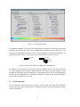
The display component can load such a file and display the different dimensions of the performance
space using three coupled tree browsers (Figure 1). The browsers are connected so that the user
can view one dimension with respect to another dimension. For example, the user can click on a
particular metric and see its distribution across the call tree. In addition, the display is augmented
with a source-code display that shows the exact position of a call site in the source code.
The following sections will explain how to install
write CUBE files.
CUBE,
how to use the display, and also how to
2 Installation
is available as a source-code distribution. You can use the link http://icl.cs.utk.
edu/kojak/cube/ to download CUBE. There are two options to install CUBE: full installation
and installation of the library only. The current version of CUBE 1.0 is able to run on all major UNIX
variants.
CUBE
5
2.1 Platforms
currently supports all major UNIX platforms on which wxWindows and libxml2 are available.
Note that libxml2 or wxWindows may require a specific compiler on some platforms.
CUBE
2.2 Installing CUBE
The full installation includes the CUBE library to write a CUBE file, and the CUBE display component
to display its contents.
1. gunzip cube.tar.gz
tar xvf
2. cd cube-xxxx
3. Edit Makefile.defs
Set variable PREFIX to your desired installation path.
Choose an appropriate compiler for your system (e.g., gcc or xlC ).
4. make
5. make install
2.3 Installing CUBE Library only
The partial installation will only install the CUBE library on your system. This is intended for users
who just need to write their performance data to a CUBE file, but don’t need to display it on their
machines.
1. Same as steps of 1 to 3 described in the above section.
2. make lib
3. make install-lib
2.4 License
This software is free but by downloading and using it you automatically agree to comply with the
license agreement. You can read the file LICENSE in the distribution for precise wording.
2.5 Libraries Required
Both libraries listed below are necessary for using the CUBE display component. For those users
who need the CUBE library only, only libxml2 is required to be installed.
6
LIBXML 2: an XML C parser and toolkit developed for the Gnome project. It is preinstalled
on many systems. Please refer to the libxml2 web page for details:
http://xmlsoft.org/
WX W INDOWS:
a cross-platform C++ framework for writing advanced GUI applications using native controls. Please refer to the wxWindows web page for details:
http://www.wxwindows.org/
3 Using the Display
This section explains how to use the CUBE display component. After a brief description of the basic
principles, different components of the GUI will be described in detail.
3.1 Basic Principles
The CUBE display consists of three tree browsers, each of them representing a dimension of the
performance space (Figure 1). The left tree displays the metric dimension, the middle tree displays
the call-tree dimension, and the right tree displays the location dimension. The nodes in the metric
tree represent performance metrics. The nodes in the call-tree dimension represent call paths. The
nodes in the location dimension represent a group of machines, called a grid, a machine, a node, a
process, or a thread.
Users can perform two types of actions: selecting a node or expanding/collapsing a node. At any
time, there are two nodes selected, one in the metric tree and the other in the call tree. It is not
possible to select a node in the location tree.
Each node is associated with a metric value, which is called the severity and is displayed simultaneously using a numerical value as well as a colored square. Colors enable the easy identification of
nodes of interest even in a large tree, whereas the numerical values enable the precise comparison
of individual values. A value shown in the metric tree represents the sum of a particular metric for
the entire program, that is, across all call paths and all locations. A value shown in the call tree represents the sum of the selected metric across all locations for a particular call path. A value shown
in the location tree represents the selected metric for the selected call path and a particular location.
Briefly, a tree is always an aggregation of all of its neighbor trees to the right.
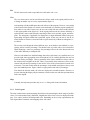
Note that all the hierarchies in CUBE are inclusion hierarchies, meaning that a child node represents
a part of the parent node. For example, the metric hierarchy might display cache misses as a child
node of cache accesses because the former event is a subset of the latter event. Similarly, in Figure
2 the call path main contains the call paths main-foo and main-bar as child nodes because their
execution times are included in their parent’s execution time.
The severity displayed in CUBE follows the principle of single representation, that is, within a tree
each fraction of the severity is displayed only once. The purpose of this display strategy is to
have a particular performance problem to appear only once in the tree and, thus, help identify it
more quickly. Therefore, the severity displayed at a node depends on the node’s state, whether it
7
Figure 1:
CUBE
display window.
is expanded or collapsed. The severity of a collapsed node represents the whole subtree associated
with that node, whereas the severity of an expanded node represents only the fraction that is not
covered by its descendants because the severity of its descendants is now displayed separately. We
call the former one inclusive severity, whereas we call the latter one exclusive severity.
100 main
10 main
30 foo
60 bar
Figure 2: Node of the call tree in collapsed or expanded state.
For instance, a call tree may have a node main with two children main-foo and main-bar (Figure
2). In the collapsed state, this node is labeled with the time spent in the whole program. In the
expanded state it displays only the fraction that is spent neither in foo nor in bar. Note that the label
of a node does not change when it is expanded or collapsed, even if the severity of the node changes
from exclusive to inclusive or vice versa.
3.2 GUI Components
The GUI consists of a menu bar, three tree browsers, a color legend, and a status bar. In addition,
each tree browser provides a context menu for each node, which can be used, for example, to launch
a source-code dialog.
8
3.2.1
Tree Browsers
The tree browsers are controlled by the left and right mouse buttons. The left mouse button is used
to select or expand/collapse a node. The right mouse button is used to pop up a context menu with
node-specific information for either a metric or a call path. For call paths and source-code entities a
source-code dialog is provided.
A label in the metric tree shows a metric name. A label in the call tree shows the last callee of a
particular call path. If you want to know the complete call path, you must read all labels from the
root down to the particular node in which you are interested. After switching to the region-profile
mode (see below), labels in the middle tree denote modules or regions depending on their levels. A
label in the location tree shows the name of its respective location entity, such as a node name or a
machine name. Processes and threads are usually identified by a number, but it is possible to give
them specific names when creating a CUBE file.
Note that both the metric tree and the call tree can have multiple root nodes. If there is only one
machine in the location tree, the grid level is not displayed. Similarly, the thread level of singlethreaded applications is hidden.
3.2.2
Menu Bar
The menu bar consists of three menus, a file menu, a view menu, and a help menu.
Figure 3:
CUBE
9
menu bar.
File
The file menu can be used to open and close a file and to exit CUBE.
View
The view menu can be used to switch from the call-tree mode to the region-profile mode or
to change to another way of severity representation (Figure 3).
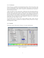
After opening a file the middle pane shows the call tree of the program. However, a user might
wish to know which fraction of a metric can be attributed to a particular region regardless of
from where it was called. In this case, the user can switch from the call-tree mode (default)
to the region-profile mode (Figure 4). In the region-profile mode, the call-tree hierarchy is
replaced with a source-code hierarchy consisting of three levels: module, region, and subregions. The subregions, if applicable, are displayed as a single child node labeled subregions
representing all regions called from a particular region. In this way, the user is able to see
which fraction of a metric is associated with a region exclusively without its subregions (i.e.,
its callees).
The severity can be displayed in three different ways: as an absolute value (default), as a percentage, and as a relative percentage. The absolute value is just the value as it was measured.
When displaying a value as a percentage, the percentage refers to the value shown at the root
of the metric hierarchy in collapsed state.
However, both modes have the disadvantage that values can become very small the more you
go to the right, since aggregation occurs from right to left. To avoid this problem, the user can
switch to relative percentages. Then, a percentage in the right or middle tree always refers to
the selection in the neighbor to the left. That is, a percentage in the location tree refers to the
selected call path and a percentage in the call tree refers to the selected metric instead of its
root metric. Note that in this mode the percentages in the middle and right tree always sum
up to one hundred percent. Figure 4 shows a region profile with relative percentages.
Note that in the absolute mode, all values are displayed in scientific notation. However, to
prevent cluttering the display only the mantissa is shown at the trees with the exponent shown
at the color legend.
Help
Currently, the help menu provides only an About dialog with release information.
3.2.3
Color Legend
The color is taken from a spectrum ranging from blue to red representing the whole range of possible
values. To avoid an unnecessary distraction, insignificant values close to zero are displayed in dark
gray. Zero values just have the background color. Depending on the severity representation, the
color legend shows a numeric scale mapping colors onto values.
10
3.2.4
Status Bar
The first column showing indicates that there are at most threads in the execution.
Figure 4:
CUBE
processes and for each process there are
region profile.
4 Creating CUBE Files
The CUBE data format in an XML instance [3]. The corresponding XMLSchema specification [4]
can be found in doc/cube.xsd in the CUBE distribution. The CUBE library provides an interface
to create CUBE files. It is a simple class interface and includes only a few methods. This section
first describes the CUBE API and then presents a simple C++ program as an example of how to use
it.
4.1 CUBE API
The class interface defines a class Cube. The class provides a default constructor and thirteen
methods. The methods are divided into four groups. The first three groups are used to define the
three dimensions of the performance space and the last group is used to enter the actual data. In
addition, an output operator << to write the data to a file is provided.
11
The methods used to create the different entities of the performance space always return an identifier
which can be used for further reference. Each entity has a different identifier domain .
4.1.1
Metric Hierarchy
This group refers to the metric dimension of the performance space. It consist of a single method
used to build metric trees. Each node in the metric tree represents a performance metric. Metrics have different units of measurement. The unit can be either “sec” (i.e., seconds) for time
based metrics, such as execution time, or “occ” (i.e., occurrences) for event-based metrics, such as
floating-point operations. During the establishment of a metric tree, a child metric is usually more
specific than its parent, and both of them have same unit of measurement. Thus, a child performance
metric has to be a subset of its parent metric (e.g., system time is a subset of execution time).
int def met(string name, string uom, string descr,
int parent id)
Defines a new performance metric with metric name name and description descr. uom
specifies the unit of measurement, which is either “sec” or “occ”. parent id is the
identifier of a previously created metric which will be the new metric’s parent. To define a
root node, use -1 instead.
4.1.2
Call-Tree Hierarchy
This group refers to the call-tree dimension of the performance space. The entities present in this
dimension are module, region, call site, and call-tree node (i.e., call paths). A module is a source
file, which can contain several code regions. A region can be a function, a loop, or a basic block.
Each region can have multiple call sites from which the control flow of the program enters a new
region. Although we use the term call site here, any place that causes the program to enter a new
region can be represented as a call site, including loop entries. Correspondingly, the region entered
from a call site is called callee, which might as well be a loop. Every call-tree node points to a call
site. The actual call path represented by a call-tree node can be derived by following all the call sites
starting at the root node and ending at the particular node of interest. Therefore, before defining a
call-tree node, the necessary call sites, callees, and modules have to be defined.
int def module(string name)
Defines a new module with module name name, which could be either a complete path or a
file name.
12
int def region(string name, long begln, long endln,
string descr, int mode id)
Defines a new region with region name name and description descr. The region is located
in the module mod id and exists from line begln to line endln.
int def csite(int mod id, int line, int callee id)
Defines a new call site which is located at the line line of the module mod id. The call site
calls the callee (i.e., a previously defined region) whose identifier is equal to callee id.
int def cnode(int csite id, int parent id)
Defines a new call-tree node referring to the call site csite id. parent id is the identifier
of a previously created call-tree node which will be the new one’s parent. To define a root
node, use -1 instead.
4.1.3
Location Hierarchy
This group refers to the location dimension of the performance space. The entities present in this
dimension are grid, machine, node, process, and thread, which populate five levels of the location
hierarchy in the given order. That is, the first level has one grid, the second level has multiple
machines, and so on. Finally, the last (i.e., leaf) level is populated only by threads. A location tree
is built in a top-down way starting with a grid. Note that even if every process has only one thread,
users still need to define the thread level. Note that different from the previous two dimension, the
location dimension can have only one root, that is, one grid.
int def grid(string name)
Defines a grid which has the name name. Note that only one grid can be defined.
int def mach(string name, int grid id)
Defines a new machine which has the name name and which belongs to the grid grid id.
int def node(string name, int mach id)
Defines a new (SMP) node which has the name name and which belongs to the machine
mach id.
13
int def proc(string name, int node id)
Defines a new process which has the name name and which belongs to the
node id.
SMP
node
int def thrd(string name, int proc id)
Defines a new thread which has the name name and belongs to the process proc id.
4.1.4
Severity Mapping
After the establishment of the three dimensional performance space, users can assign severity values
to points of the the space. Each point is identified by a tuple (met id, cnode id, thrd id).
Note that the value should refer exclusively to the call path denoted by cnode id and not to its
children. Taking Figure 2 as an example, this mean that if it refers to main then it does not include
main-foo or main-bar. The default severity value for the data points left undefined is zero. Thus,
users only need to define non-zero data points.
void set sev(int met id, int cnode id, int thrd id,
double value)
Assigns a value to the point (met id, cnode id, thrd id).
void add sev(int met id, int cnode id, int thrd id,
double value)
Adds a value to the existing value of point (met id, cnode id, thrd id).
void sub sev(int met id, int cnode id, int thrd id,
double value)
Subtracts a value from the existing value of point (met id, cnode id, thrd id).
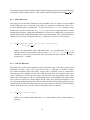
4.2 Typical Usage
A simple C++ program is given to demonstrate how to use the CUBE write interface. Figure 5
shows the corresponding CUBE display. The source code of the target application is provided in
Figure 6.
14
Figure 5: Display of example.cube
1
10
11
20
21
60
80
100
void foo() {
...
}
void bar() {
...
}
int main(int argc, char* argv) {
...
foo();
...
bar();
...
}
Figure 6: Target-application source code example.c
// A C++ example using CUBE write interface
int main(int argc, char* argv[]) {
// Declarations (all int)
int id;
...
Cube cube;
// Build metric tree
id0 = cube.def_met("Time", "sec", "root node", -1);
id1 = cube.def_met("User time", "sec", "2nd level", id0);
id2 = cube.def_met("System time", "sec", "2nd level", id0);
15
// Build call tree
id = cube.def_module("/ICL/CUBE/example.c");
id0 = cube.def_region("main", 21, 100, "1st level", id);
id1 = cube.def_region("foo", 1, 10, "2nd level", id);
id2 = cube.def_region("bar", 11, 20, "2nd level", id);
id3 = cube.def_csite(id, 21, id0);
id4 = cube.def_csite(id, 60, id1);
id5 = cube.def_csite(id, 80, id2);
id0 = cube.def_cnode(id3, -1);
id1 = cube.def_cnode(id4, id0);
id2 = cube.def_cnode(id5, id0);
// Build location tree
id0 = cube.def_grid("Grid in ICL");
id0 = cube.def_mach("msc", id0);
id0 = cube.def_node("athena", id0);
id0 = cube.def_proc("Process 0", id0);
cube.def_thrd("Thread 0", id0);
cube.def_thrd("Thread 1", id0);
// Severity mapping
cube.set_sev(0, 0, 0,
cube.set_sev(0, 0, 1,
cube.set_sev(0, 1, 0,
cube.add_sev(0, 1, 1,
cube.add_sev(0, 2, 0,
cube.add_sev(0, 2, 1,
cube.set_sev(1, 0, 0,
cube.set_sev(1, 0, 1,
cube.set_sev(1, 1, 0,
cube.add_sev(1, 1, 1,
cube.add_sev(1, 2, 0,
cube.add_sev(1, 2, 1,
cube.set_sev(2, 0, 0,
cube.set_sev(2, 0, 1,
cube.set_sev(2, 1, 0,
cube.add_sev(2, 1, 1,
cube.add_sev(2, 2, 0,
cube.add_sev(2, 2, 1,
4);
4);
4);
4);
4);
4);
1);
1);
1);
1);
1);
1);
1);
1);
1);
1);
1);
1);
// Output to a cube file
ofstream out;
out.open("example.cube");
out << cube;
}
16
References
[1] Message Passing Interface Forum. MPI: A Message Passing Interface Standard, June 1995.
http://www.mpi-forum.org.
[2] OpenMP Architecture Review Board. OpenMP Fortran Application Program Interface - Version 2.0, November 2000. http://www.openmp.org.
[3] World Wide Web Consortium. Extensible Markup Language (XML) 1.0 (Second Edition), October 2000. http://www.w3.org/TR/REC-xml.
[4] World Wide Web Consortium. XML Schema Part 0, 1, 2, May 2001. http://www.w3.
org/XML/Schema#dev.
17


![the file [< 1 MB]](http://vs1.manualzilla.com/store/data/005663565_1-91d1e4bcdfd7b45b626a6b88ab809728-150x150.png)