Download User Manual Release 2.1

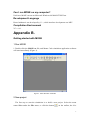
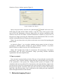
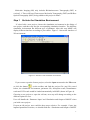
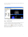
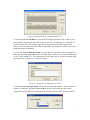
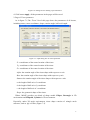
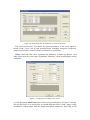
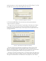
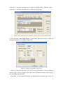
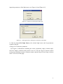
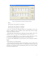
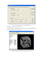
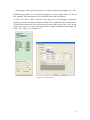
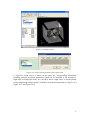
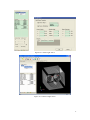
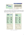
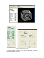
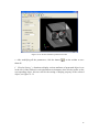
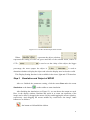
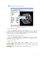
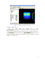
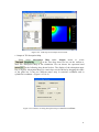
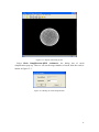
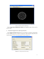
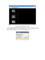
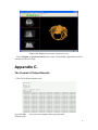
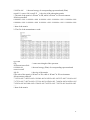
MOLECULAR IMAGE GROUP, LIFE SCIENCE RESEARCH CENTER, XIDIAN UNIVERSITY, XIAN, P.R.C. MEDIAL IMAGE PROCESSING GROUP, INSTITUTE OF AUTOMATION, CAS, BEIJING, P.R.C. VT‐WFU SCHOOL OF BIOMEDICAL ENGINEERING & SCIENCES, VIRGINIA, U.S.A. MOSE Molecular Optical Simulation Environment User Manual
Release 2.1
[Service e-mail: [email protected]]
Appendix A. ...................................................................................................................................2
Introduction ...........................................................................................................................2
How to input the parameters? ..........................................................................................2
How does MOSE simulate? ...............................................................................................2
Can I run MOSE on my computer? ..................................................................................3
Development Language......................................................................................................3
Compilation Environment ..................................................................................................3
Appendix B. ...................................................................................................................................3
Getting started with MOSE ................................................................................................3
1 Molecular Imaging Project .................................................................................4
Step 1 Get into the Simulation Environment..............................................5
Step 2 Parameter Input ....................................................................................6
Step 3 Simulation and Output of MOSE ....................................................21
2 Image Processing Project..................................................................................28
Appendix C. .................................................................................................................................32
The Format of Output Results ........................................................................................32
Appendix D. .................................................................................................................................34
FAQ ........................................................................................................................................34
1
Appendix A.
Introduction
MOSE is a photon tracing program for optical analysis of biological tissue models.
MOSE traces photons using “Monte Carlo Technique”.
The best way to describe how does MOSE work might be to briefly outline the
steps that are typically taken if you were to start a new MOSE project. These steps
will be discussed in the following sections.
If you are beginning to create a new MOSE project, it needs to choose and create
the appropriate type project on the specific function, MOSE includes two different
types of projects, "BLT" and "image processing". You will enter in different operating
interface according to the type of project. The following will define the different types
of projects in detail.
How to input the parameters?
MOSE has a very friendly user interface. There are a number of ways to input data
and output results for users.
Take the BLT project for example, it offers two efficient approaches for us to input
the parameters. One is loading the parameter files (.mse file), which has a specified
form. We will offer some standard parameter files to users to study how to construct
the parameter file. The other is inputting the parameters in the parameter setting
dialog box. No matter which approach, you can simply modify parameters after
inputting. You can add or delete tissues or light sources or detectors if you need. It is
especially useful when the kinds of tissues or light sources or detectors are more than
the default settings.
How does MOSE simulate?
After inputting the parameters, we can start the BLT simulation or the image
processing.
Take the BLT project for example. Monte Carlo (MC) method constructs the
foundation of the BLT, and in the MC method the source was discretized into a
number of photon packets. The whole propagation of each photon packet includes
three main parts: photon packet generation from bioluminescent sources, the
propagation in biological tissues and detection by the CCD detectors, which were
completed through the Monte Carlo (MC) method. The MC method has been proved
to be exact and efficient. During the whole process, MOSE not only traces the travel
paths of each photon packet but also records the absorption and transmittance
information. With these records, MOSE can give absorption and flee map of the
photons in phantom.
2
Can I run MOSE on my computer?
Until now, MOSE can run on Microsoft Windows 98/2000/NT/XP/Vista.
Development Language
Kernel arithmetic was developed by C++, while interface development was MFC.
Compilation Environment
VC++ 6.0.
Appendix B.
Getting started with MOSE
1 Run MOSE
1. Double click the MOSE.exe file, and Monte Carlo simulation application software
will start immediately (Figure 1).
Figure 1. Main Window of MOSE
2 New project
The first step to start the simulation is to build a new project. Select the menu
named New under the File menu, or click the button
on the toolbar, the New
3
Simulation Project window appears (Figure 2).
Figure 2. Build a New Project
Input your project name, select the save path through
, MOSE will create a new
folder under the path and the folder include a .mpj file.( Note: In the project of the
type of BLT, the information of tissues, light sources etc and the simulation results
could be saved in the file folder. And this information is related by a project file. In
the project of image processing, the information is not related because there is no such
absolute relationship between image process and output data.)
Where, the user must select save path to avoid some errors caused by inputting path
hand manual.
As shown in figure 2, we can select simulate project pattern in item of project,
according to different pattern, MOSE can appear different interface. At present,
MOSE include two kinds of project: BLT and image process.
Where, BLT includes three kinds of environment: 2D environment, 3D analytic
environment and 3D mesh environment. Image processing includes threshold
segmentation and mesh simplification.
3 Open a project
Users can open a project built previously. The type of .mpj and other associated file,
could also be open. And the interface would show the corresponding state according
to the parameters of the project file. Taking the BLT project as example, if the
simulation had been run and the files of parameters and results had been output in the
previous project, these files of parameters and results would be opened together when
the project was opened. And it may take some time to do this procedure when loading
huge data. After this procedure, users could observe the results got by the simulation
before through the buttons on the interface.
1 Molecular Imaging Project
4
Molecular Imaging (MI) only includes Bioluminescence Tomography (BLT) at
version 2.1. There will have Fluorescence Molecular Tomography (FMT) and Diffuse
Optical Tomography (DOT) being added to this project in future.
Step 1
Get into the Simulation Environment
If select built a new project, choose the simulation environment in the dialog of
new project, and then step into the corresponding simulation interface. The different
simulation environment has different type of phantom. After this step MOSE will
display different interface according to your choice. Figure 3-1 shows the interface of
2D environment.
Figure 3-1.Interface of 2D simulation environment
If you want to open the former project, select the Open menu under the File menu
or click the button
on the toolbar, and find the project file (.mpj file) saved
before, the simulation environment, parameter file, absorption result, transmittance
result and CCD result would be loaded automatically in MOSE (shown in Figure 4).
Choosing a new project or open the old one, next step will change according to the
different option for user.
User will handle the ‘Parameter Input’ and ‘Simulation and Output of MOSE’ when
you built a new project.
If open an old project, user could do these steps selective. For example, if user just
inputted parameters last time, we should finish the ‘‘Simulation and Output of MOSE’
5
step; if not, we will restart it. If all the two steps were done, what we should do is just
to open it and get the result.
Figure 4 . Open a BLT project that is in 3D mesh environment
Step 2
Parameter Input
1. The steps of inputting the parameter in these three simulation environments are
similar. Here, we just take the 3D analytic environment as the example.
As in Figure 3-2, in the main window, under the input menu, click 3D Analytic
Parameter or click the button
. The Input Parameters window appears (See
Figure 5). There are four different input pages named ‘Tissue’, ‘Light Source’ ‘CCD’
and ‘MC simulation’, respectively.
6
Figure 5. Input dialog box for simulation parameters
a. Click the button Load Data, we can load 3D analytic parameter file (*.mse/*.txt)
from outside. We provide some file examples for user to study how to use MOSE. If
the form of the file is not correct, only the correct parameters will be read in and
others need to be input manually. After loading data, the parameter will be seen in the
Input Parameters dialog box.
b. Click the button Add Spectrum, we can add new spectrum band as Figure 6-1
indicates. Also the optical parameter of all the tissues in the new spectrum band could
be set in this dialog box. The information of the light sources in this spectrum band
could be set in ‘Light Source’ Parameter Page.
Figure 6-1. Dialog box for adding spectrum band
c. Click the button Del Spectrum, choose the spectrum band that we want to delete as
Figure 6-2 indicates, and press Button OK to delete it. After this step the tissues
parameters and the light sources parameters related to this spectrum will be deleted.
7
Figure 6-2. Dialog box for deleting a spectrum band
d. Click button Apply, all the parameters in the pages will be saved.
2. Page of Tissue parameter
As in figure 7-1,The ‘Tissue’ list of this page shows the parameters of all tissues,
including name, center coordinates, shape, rotation angle, half-axis length.
Figure 7-1. Input dialog box for tissue parameter
X: x coordinates of the center location of the tissue
Y: y coordinates of the center location of the tissue
Z: z coordinates of the center location of the tissue
Alpha: the rotation angle of the tissue shape with respect to x-axis
Beta: the rotation angle of the tissue shape with respect to y-axis
Gamma: the rotation angle of the tissue shape with respect to z-axis
a: the length of half axis of x coordinate
b: the length of half axis of y coordinate
c: the length of half axis of z coordinate
Shape: the geometric shape of the tissue.
Where, MOSE provides two kinds of shape model: Ellipse, Rectangle in 2D
environment and Ellipsoid, Cylinder in 3D environment.
Especially, under 3D mesh environment, tissue shape consists of triangle mesh
structure, such as .ply/.off files (Figure 7-2).
8
Figure 7-2. Input dialog box for parameter of tissues in 3D mesh
The ‘Optical Parameter’ list shows the optical parameters of the tissue which is
chosen in the ‘Tissue’ list in each spectrum band, including absorption coefficient,
scattering coefficient, refractive index, and anisotropy coefficient.
Notice: Since the first tissue represents the phantom, it cannot be deleted. And
other tissues must be in the range of phantom. Otherwise, errors would happen during
simulation.
Figure 7-3. Dialog box for adding a new tissue
a. Click the button Add Tissue, there will be an input dialog box as Figure7-3 shown.
We can add tissue as we need. Here we should input the tissue’s name, shape, center
coordinates, rotation angle, half axis length and optical parameters. Especially, in 3D
9
mesh environment, we need to input the path of the .ply/.off files (Figure 7-4). Click
the ‘OK’ button, the new tissue will be added in the ‘Tissue’ list.
Figure 7-4. ‘Add Tissue’ dialog box in 3D mesh
b. Click the button Del Tissue, delete selected tissue and its optical parameters.
3. Page of Light Source parameter
This page consists of the information of regular shape of the light sources (Figure
8-1). As the tissue page, the upper list shows the information of the light sources,
including the center coordinates, shape, rotation angle, half-axis length and the form
of energy distribution.
Figure 8-1. Input dialog box for light source parameter
The lower list shows the information of the light source which is chosen in the
upper list, including the photon energy and photon number of the light source in
different spectrum band. Here, if the light source doesn’t include one of the spectrum
bands, the corresponding photon number and energy should be set to zero.
Especially, in 3D mesh environment, there’re two kinds of shape of the light source.
One is analytic shape (ellipsoid, cylinder), the other is mesh shape (mc triangle mesh).
The upper list mentioned above is divided into two lists (Figure 8-2). The ‘Analytic
10
Light Source’ list shows the light sources which are analytic shape, while the ‘Mesh
Light Source’ list shows the light sources which are mesh shape.
Figure 8-2. Input dialog box for parameter of light sources in 3D mesh environment
a. Click the button Add Light Source, regular shape light source will be added and
the input dialog box is as follows (Figure 8-3):
Figure 8-3. Dialog box for adding a light source
Where, we should set the shape, the form of energy distribution, center coordinates,
rotation angle, half-axis length of the light source and photon number and energy in
corresponding spectrum band.
Especially, in 3D mesh environment, we should select the shape type before we
11
input the parameters of the light source (see Figure 8-4 and Figure 8-5).
Figure 8-4. Dialog for selecting the shape type
Figure 8-5. ‘Add Light Source’ dialog box if select the mesh shape
b. Click the button Del Light Source, the selected light source and its parameters
would be deleted.
4. Page of CCD detector parameter
See Figure 9, information, including the center coordinates, shape, rotation angle,
half axis length, resolution and normal vector of CCD, the flag for detector matrix
saving, the coordinate system of detector matrix and the flag for lens being, is shown
in the ‘CCD’ list of this page.
12
Figure 9. Input dialog box for parameter of detectors and lens
Where,
Resolution(dx): the resolution of x coordinate
Resolution(dy): the resolution of y coordinate
Resolution(dz): the resolution of z coordinate
The ‘Lens’ list shows the information about lens corresponding to each of the
detectors, including the center coordinates, shape, rotation angle, half axis length,
normal vector and focus of the lens.
If the last item ‘Lens’ item in the ‘CCD’ list set to be “nolens”, all the lens
parameters in the ‘Lens’ list for the corresponding detector will be set to zero.
a. Click the button Add CCD, a new row for detector would be added into the ‘CCD’
list. And the corresponding parameters information can be inputted by user.
b. Click the button Del CCD, the selected detector and its information would be
deleted.
5. Page of Monte Carlo (MC) parameter
The information about absorption matrix and transmittance matrix for Monte Carlo
simulation is illustrated in this page (Figure 10), including the coordinate system and
resolution of the absorption matrix and transmittance matrix. We can choose whether
to save the two matrixes or not.
13
Figure 10. Input dialog box for MC simulation parameter
6. Modification of the parameter in sidebar
After the parameters in four pages are all inputted, click the button OK then enter
the simulation interface (shown in Figure 11).
Figure 11. Interface of simulation in 3D analytic environment
14
In this image, white represents tissues, red represents light source and gray is CCD.
Unfolding the sidebar, we can find the parameters of tissue, light source, CCD and
MC inputted. These parameters can be modified easily and flexibly here.
a. Tissue list: Tissue name is shown in the upper list, corresponding information
including position and shape parameters which can be modified in the second list (in
3D mesh environment, the second list shows the path of the .ply/.off file). We can add
tissue, delete tissue, or set the optical parameter by right clicking the tissue name (see
Figure 12-1, Figure 12-2, Figure 12-3).
Figure 12-1. Add a tissue
15
Figure 12-2. Delete a tissue
Figure 12-3. Set the optical parameters of the light source
b. Light list: Light source is shown in the upper list, corresponding information
including position and shape parameters which can be modified in the second list.
Right click a certain light source, we can add or delete a light source, or set the photon
energy distributing and the number of photons in each spectrum band (see Figure 12-4,
Figure 12-5, and Figure 12-6).
16
Figure 12-4. Add a light source
Figure 12-5. Delete a light source
17
Figure 12-6. Set the property of the light source
c. CCD List: All the detectors are shown on the upper list, corresponding information
including position and shape parameters which can be modified in the second list.
Right click a certain detector, we could add or delete a detector or set the parameters
of lens (see Figure 12-7, Figure 12-8, Figure 12-9).
Figure 12-7. Add a CCD detector
18
Figure 12-8. Delete a CCD detector
Figure 12-9. Set the parameters of lens
d. MC parameter page: see Figure 12-10, we can set the information of absorption
and transmittance matrix in this page.
19
Figure 12-10. Set the simulation parameter for MC
e. After modifying all the parameters, click the button
on the toolbar to save
them all.
f. ‘Display Setting’, a function to display various attributes of protracted object is set
in the area of the sidebar in each simulation environment, when left-key strike on the
corresponding object, this area will be the setting of display property of the selected
object, see figure 12-11:
20
Figure 12-11. Set the simulation parameter for MC
Where,
represents the object selection;
represents the setting of color red, green and blue of the selected tissue, source or
CCD ;
is used to set the clarity of the object, the bigger
percentage, the more opaque the object is.
is used to
determine whether to display the object and select the display state in closed or solid.
This Display Setting function is also available in the tissue, light and CCD interface
Step 3
Simulation and Output of MOSE
After we finished the parameters setting, click the menu Run under the menu
Simulation or the button
on the toolbar to start simulation.
After finishing the simulation (see Figure 13), we can choose the output we need.
Here, in the display window, Rotation and zoom in or zoom out operation of the
image can be done by dragging the mouse left key and dragging the mouse right key,
respectively. And dragging the mouse middle key could move the image. Other
buttons are as follows:
: the button to fold/unfold the sidebar
21
: the button to reset the coordinate axis
Figure 13. Simulation is over
a. Output of Simulation Parameter
Select menu Simulation parameter under Output menu, we can save the
parameters, including the tissues, the light sources, the detectors and the simulation
parameter for MC, in the form of standard parameter file (.mse file), which will be
saved into current project folder for simulation in future.
b. Output of simulation results for Monte Carlo
Select menu 3D Simulation Result under Output menu, the absorption matrix,
transmittance matrix and detection matrix of the Monte Carlo simulation could be
saved to the current project folder.
c. Output of 3D Flee Map
Select
menu
Flee
Map
under
Output
menu
or
select
in the first drop down list box on the toolbar, we can
see the Flee Map of this simulation. And we can select the spectrum band
in the following drop down list box (See Figure 14-1).
22
Figure 14-1. Flee map in 3D analytic environment
d. Output of 3D CCD Map
Select
Map
under
Output
menu
or
select
in the first drop down list box on the toolbar to show
the map on CCD. In the following drop down list box we can choose the spectrum
band
menu
CCD
. The drop down list box
select the serial
number of detector, the order of the serial number is same as the detector in input
parameters: (see Figure 14-2).
23
Figure 14-2. CCD map in 3D analytic environment
e. Output of 3D Absorption Map
Select
menu
Absorption Map under Output menu or select
in the first drop down list box on the toolbar to
show the Absorption Map of the simulation. We can choose the spectrum band
in the following drop down list box. The display of the absorption maps
here is layered. Absorption Map of a certain layer can be shown by dragging the slider
of the glide bar. It has two different maps: map in cartesian coordinate and in
cylindrical coordinate . (Figure 14-3,14-4)
Figure 14-3. Interface of setting absorption map in cartesian coordinate
24
Figure 14-4. Interface of setting absorption map in cylindrical coordinate
Select Single layer, the absorption map is displayed in single layer model, select
layers in the glide bar
. In cartesian coordinate, X-Y option
means layer selection is paralleling x-y axis, so Y-Z, Z-X means the selection
paralleled y-z and z-x axis in the same way. Selecting the option along z-axis means
that the mode of layer-selecting is spar sampling paralleled to z-axis, selecting the
option Perpendicular to z-axis means that the mode of layer-selecting is ellipsoidal
sampling vertical to z-axis.
Here, there are two kinds of absorption maps: one if them is paralleling to x-y axis
in cartesian coordinate and the other is vertical to z-axis in cylindrical coordinate
(Figure 14-5,14-6)
Figure 14-5.Single absorption map parallel to xy-axis in cartesian coordinate
25
Figure 14-6.
Single absorption map vertical to z-axis in cylindrical coordinate
Select Multiple layers, the absorption map will be displayed in Multiple layers
model. Set layers in the dialog box
with the space between
them, then the absorption maps of the layers are appeared, shown in figure 14-7, 14-8
14-9,14-10. Similar to Slice plane.
Figure14-7. Interface of setting multiple layers absorption map in cartesian coordinate
26
Figure14-8. Interface of setting multiple layers absorption map in cylindrical coordinate
Figure 14-9. Multiple absorption map vertical to z-axis in cylindrical coordinate
27
Figure 14-10. Multiple absorption map parallel to xy-axis in cartesian coordinate
2
Image Processing Project
When image processing was chosen, the corresponding interface appears, which
includes two functions: “Threshold Segmentation” and “Mesh Simplification”.
a
Mesh simplification and Output Results
Select Input-Load Data-ply file load .ply or .off file outside, shown in figure 15-1
after loaded:
28
Figure 15-1 Display after load ply file
Select Mesh Simplification-QEM Arithmetic, the dialog box of mesh
simplification pops up. Then we can set the target number of mesh, then the result is
shown in figure 15-3:
Figure 15-2 Dialog for mesh simplification
29
Figure 15-3 Result of mesh simplification
Select Output-Mesh Simplification Result, the simplified results will be saved in
the file of ply.
b
Threshold Segmentation and Output Results
Select Input-Load Data-raw file load .raw file outside, a parameter setting dialog
for file inputting pops up, as shown in Figure16-1.Then click the button OK, the
interface appears if file is correctly inputted, shown in Figure16-2:
Figure 16-1. Dialog for parameter setting
30
Figure 16-2. Display after input raw file
Select Segmentation–Threshold Segmentation, the dialog box of setting threshold
pops up (shown in figure 16-3). After setting upper and lower threshold, we will
obtain the threshold segmentation result, shown in figure 16-4:
Figure 16-3. Dialog for setting threshold
31
Figure 16-4. Display for threshold segmentation result
Select Output- Segmentation Result, the results of threshold segmentation will be
outputted in the file of ply.
Appendix C.
The Format of Output Results
1. The file of the absorption result
spectrum 400
3DAbosrption
// the center wavelength of the spectrum band
32
2.99970e-001
// the total energy of corresponding spectrum band (Watt)
countR 11 countA 360 countZ 23 // the size of the absorption matrix
// The unit of the matrix is W/mm2 in 2D, while is W/mm3 in 3D environment.
3DAbsorptionRAZ
0.00000e+000 0.00000e+000 0.00000e+000 0.00000e+000 0.00000e+000
0.00000e+000 0.00000e+000 0.00000e+000 0.00000e+000 0.00000e+000
……
// data of the matrix
2. The file of the transmittance result
spectrum
620
// center wavelength of the spectrum
3DTransmittanceSide
8.89940e-00
// the total energy (Watt) of corresponding spectrum band
countA countZ
360 20
// the size of the matrix
//The unit of the matrix is W/mm2 in 2D, while is W/mm3 in 3D environment.
3DtransmittanceSideAZ
7.19233e-002 7.00232e-002 6.30366e-002 6.98502e-002 6.65337e-002 7.68149e-002
7.47553e-002 7.08378e-002 6.55314e-002 8.05368e-002 7.46624e-002 6.86954e-002
7.42054e-002 6.82968e-002 6.59465e-002 7.60552e-002 7.38552e-002 8.44916e-002
……
// data of the matrix
33
3. The file of detector result
spectrum 620
// center wavelength of the spectrum
3DDetection 1
// The Num 1 is the serial number of the CCD.
1.49110e-002
// the total energy (Watt) of corresponding spectrum band
absorbed by CCD1
CountY CountZ
100 110
// the size of the matrix
// The unit of the matrix is W/mm2 in 3D environment.
3DDetectionYZ
8.29847e-006 8.55013e-006 8.81174e-006 9.08377e-006 9.36672e-006 9.66114e-006
9.96756e-006 1.02866e-005 1.06188e-005 1.09650e-005 1.13257e-005 1.17017e-005
1.20938e-005 1.25029e-005 1.29296e-005 1.33751e-005 1.38401e-005 1.43259e-005
......
// data of the matrix
Appendix D.
FAQ
1. Why the display of the phantom stay unchanged after the parameters have been
modified in the sidebar?
Answer: After modify the parameters in the sidebar, only when clicking the “save”
button on the toolbar could save the parameters meanwhile updating would be
displayed.
2. What is the meaning of different types of absorption matrix and transmission
matrix in the ‘MC Simulation Parameter’ page of the input parameter dialog box?
Answer: There are two types of absorption matrix: artesian coordinate and cylindrical
coordinate. The difference between them is to define the position of photon be
34
absorbed in cartesian coordinate or cylindrical coordinate. The different choice of
coordinate system will lead to different absorption matrix visual effect. The cartesian
coordinate form absorption matrix will display in form of slice of absorption matrix
parallel to X-Y plane. The cylindrical coordinate form absorption matrix will display
in form of slice of absorption matrix parallel to Z axis. Slices need to be observed by
glide bar. The amount of absorb is represented by color. But corresponding color bar
is not been displayed yet.
According to different simulation environment, absorption matrix has different type.
It only has polar coordinate form in 2D simulation environment, but has cartesian
coordinate form and cylindrical coordinate form in 3D analytic and mesh
environment.
Transmission matrix only has polar coordinate form in 2D simulation environment,
cylindrical coordinate form in 3D analytic environment, cartesian coordinate form in
3D analytic and mesh environment.
3. When the program is running, why clicking the left key of mouse is ineffective to
restore up a minimized program window?
Answer: You can restore up the window by clicking the restore menu on the taskbar.
4. In the 3-D mesh simulation environment, what are the meanings of
the“3DTransmittanceMeshFace”and the “3DTransmittanceMeshVertsx”
respectively?
Answer: “3DTransmittanceMeshFace” represents the emitted flux density (w/mm2)
of each triangular mesh face. “3DTransmittanceMeshVertex” represents the emitted
flux density (w/mm2) of each triangular mesh vertex. The former is the ratio between
the total weight of photons that emitted from the triangular mesh face and the area of
the triangular mesh, the later is the ratio between the total energy and total area of
triangular mesh which exists in the intersectant parts of the point, and the order of the
results of the “3DTransmittanceMeshVertex” conforms to that of the vertexes of the
outer tissue of the phantom.
5. The progress bar would shade the image of the original simulation data and make
the user couldn’t observer the data, how to handle this problem?
Answer: When the MOSE running, the progress bar is in the center of the window of
MOSE all the time and can’t be moved to other places, but the user could move the
image of the original simulation data by the left button, right button and middle button.
Moving the mouse after depressing the left button could rotate the image, or the right
button could zoom in\out the image, or the middle button could move the image in the
window.
6. Why the process of MOSE still exists in the task manager when the error appears in
some situation when running and the MOSE is closed?
Answer: Because the MOSE is still in the development. It have some bugs that can’t
35
be avoided in MOSE and that can make the execution abort unexpected, and this
caused that the memory of the MOSE isn’t released correctly. So the process of
MOSE still exists in the task management. We would solve this problem gradually in
the subsequent versions.
7. In the 3-D mesh simulation environment, why the error still happens in reading the
simulation parameters file (.mse) when the path of the file representing the tissue
shape is right?
Answer: Maybe the reason is that the path of file contains blank or some other illegal
character that can’t be identified by the computer. You need to set the path of the
shape file in the ‘Tissue Parameter’ page or ‘Light Source Parameter’ page.
36