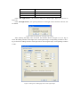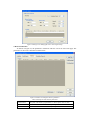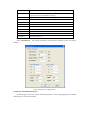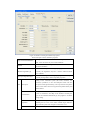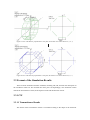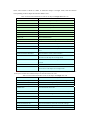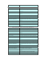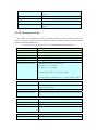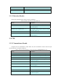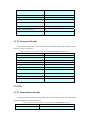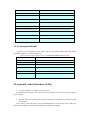
1
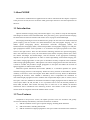
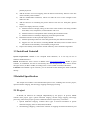
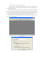
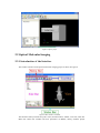
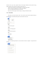
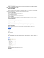
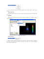
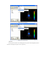
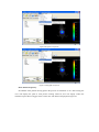
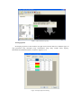
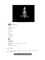
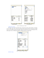
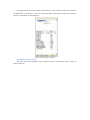
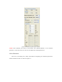
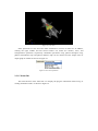
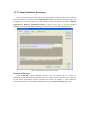
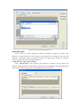
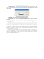
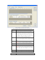
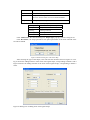
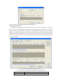
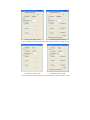
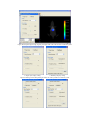
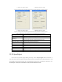
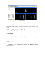
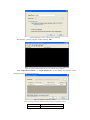
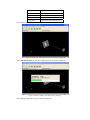
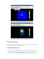
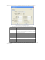
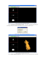
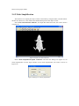
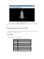
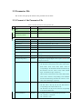
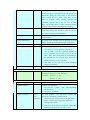
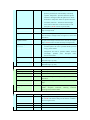
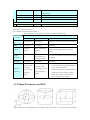
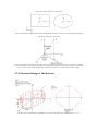
Home Page
Molecular Image Group, Life Sciences Research Center, Xidian University
Medical Image Processing Group, Institute of Automation, Chinese Academy of Sciences
Biomedical Imaging Division, School of Biomedical Engineering & Sciences, Virginia Tech–Wake Forest
University, USA
MOSE
Molecular Optical Simulation Environment
User Manual
Version 2.1.2
Last update:2010.12.24
Ge Wang, Ph. D., [email protected]
Jie Tian, Ph. D., [email protected]
Jimin Liang, Ph. D., [email protected]
Nunu Ren, Ph. D. Candidate, [email protected]
1 About MOSE
The functions of MOSE and its application areas will be introduced in this chapter. Compared
to the previous version, the new version has made great improvements to meet the requirements of
the users.
1.1 Introduction
Optical molecular imaging using near-infrared light is very useful to study the development
and changes of disease in the biomedical field. Over past twenty years, optical molecular imaging
has attracted more and more attention and made a series of progress and breakthrough.
The imaging technologies can be divided into two groups: the first is the two-dimensional (2D)
planar imaging, and the second is the three-dimensional (3D) tomographic imaging, such as
diffuse optical tomography (DOT), fluorescence molecular tomography (FMT), and
bioluminescence tomography (BLT). The forward problem of tomographic imaging is to study the
light propagation and the inverse problem is to reconstruct the optical properties of the inner
tissues or the light sources. There are three distinct technology domains for optical tomography,
that is the continuous wave (CW), the time-domain (TD) and the frequency-domain (FD). Each
has distinct advantages and disadvantages, and the selection of the appropriate technology
depends on the specific application. In order to realize high-fidelity, small-animal imaging, the
non-contact imaging approaches in free-space is introduced recently compared to the traditional
method using light-guiding fibers. Although the non-contact imaging has become the mainstream,
it needs to consider the procedure of light propagation in free-space and makes the research of
light propagation in medium more difficult.
Molecular Optical Simulation Environment (MOSE) is a simulation platform for optical
molecular imaging research co-developed by Xidian University, Institute of Automation, Chinese
Academy of Sciences, China and Virginia Tech–Wake Forest University School of Biomedical
Engineering & Sciences, USA. MOSE is featured by that it implements the simulation of
near-infrared light propagation both in medium with complicated shapes (such as mouse) and in
free-space. Until now, MOSE has realized the simulation of light propagation both in medium and
in free-space under CW, TD, and FD, so it is a powerful tool to solve the forward problems in
DOT, FMT, and BLT. This manual will help users to learn how to use MOSE, the detailed
information will be introduced in the following sections. The solution of the inverse problem
remains under investigation and will be added in future version.
1.2 New Features
Compared to the previous version, the update provides some new functions and greatly
increases the stability and efficiency. The main contents are as follows:
1) Add the simulation of two types of optical imaging, including DOT and FMT.
2) Add two domains, including TD and FD.
3) Add the simulation of light propagation in free-space under CW based on the method of
4)
5)
6)
7)
8)
9)
pinhole projection.
Add the function of reverse mapping from the fluence measured by detector to the flux
on the boundary of the medium.
Add the multithreaded simulation, which can make the most of the strengths of the
multicore CPU.
Add the function of calculating the photon fluence from the raw absorption (photon
density).
Improve the display functions, include:
a) Add the function of display setting of the tissues in the medium. The setting includes
show/hide, color, transparence, solid/wireframe and so on.
b) Add the function of interpolation while rendering the simulation results.
c) Add the function of multilayer displaying of the absorption results.
Extend the functions of file input and output, include:
a) Add the input/output function of the data generated by the different simulations.
b) Support two new file formats, including MESH and SURF, which are both used to
describe the tissue boundary constructed by triangle mesh.
Improve the stability of the software and the efficiency of the simulation algorithms.
1.3 Install and Uninstall
System requirements: MOSE is now complied under Windows, so it can only be run on
Windows 2000/XP/Vista/7.
Install: Download the latest version of MOSE from http://www.mosetm.net. MOSE is green
software, no installation, and can be used directly after the decompression. User need to choose
the right version (32-Bit or 64-Bit) according to the version (32-Bit or 64-Bit) of Windows.
Uninstall: Since MOSE is green software, you can uninstall it after deleting the folder of MOSE
directly.
2 Detailed Specification
This chapter will conduct a more detailed description of use, including four sections: project,
optical molecular imaging, 2D-3D energy mapping and image processing.
2.1 Project
In MOSE, all functions are managed independently by the project. At present, MOSE
contains three project types: optical molecular imaging, 2D-3D energy mapping and image
processing. These three project types have different functions respectively. As follows:
1. Optical Molecular Imaging: Contains three types of forward simulation of optical
molecular imaging. Such as: BLT, FMT, and DOT.
2. 2D-3D Energy Mapping: Contains the function of mapping the fluence detected by 2D
CCD to the flux on the 3D surface of the medium.
3. Image Processing: Contains threshold extraction of CT raw data and mesh simplification.
As shown in Figure 1, there are two options, including ‘New Project’ or ‘Open Project’, can
be chosen after MOSE started.
New Project: Build a new project object, as shown in Figure 2. The purpose of build project
is to facilitate unified management of the data that related to the simulation. Each individual
project is corresponding to a separate folder. Project name and project path are set freely by users.
After click OK, a project folder in the project path will be generated. The folder contains a
project file (suffix .mpj). Please do not modify the project file to avoid unknown error.
Open Project: Open an existing project object, including various data generated by the
simulation. As shown in Figure 3.
Figure 1 Start MOSE.
Figure 2 Build a new project.
Figure 3 Open a project.
2.2 Optical Molecular Imaging
2.2.1 Introduction of the Interface
The window interface of the optical molecular imaging project is shown in Figure 4.
Figure 4 Main interface of MOSE.
The interface mainly includes five parts: menu, function button, sidebar, view area, status bar.
Menu bar: Menu bar includes all basic operations of MOSE, mainly includes project
operation (new, open, close), parameter input, result output, simulation control (start and stop),
graphic display control, operation of display window and so on.
Tool bar: Some commonly used commands are arranged on the toolbar.
Side bar: All the input parameters are shown on the side bar.
View area: Display all the parameters and results.
Status bar: Show the progress while writing or reading the simulation results.
2.2.1.1 Menu Bar
The upper part of main interface ranks a list of menus. Each menu has different functions.
The followings are the detailed description of each function menu item.
·Project
New
Create a new project.
Open
Open an existing project.
Close
Close the current project.
Exit
Exit MOSE.
·Input
3D Parameter
Input the simulation parameters in 3D environment. Please see Chapter 3 for parameter file
format.
·Output
Simulation Parameter
Output the simulation parameters used in the current simulation to the constructed project
folder, the document suffixes is .MSE.
3D Simulation Result
After complete simulation, output the simulation results to the constructed project folder,
including absorption results, transmission results, and detection results.
(CW) Absorption Map
Display the photon absorption map under CW.
(CW) Transmittance Map
Display the photon transmittance map under CW.
(CW) CCD Map
Display the detection map captured by CCD (This function can only be chosen in 3D CW).
(TD) Absorption Map
Display the photon absorption map under TD.
(TD) Transmit Map
Display the photon transmittance map under TD.
(FD) Absorption Map
Display the photon absorption map under FD (Amplitude and phase, respectively).
(FD) Transmit Map
Display the photon transmittance map under FD (Amplitude and phase, respectively).
·Simulation
Start
Start simulation.
Stop
Stop the simulation during the simulation process, the program will return a warning on
failure.
·View
Toolbar
Set whether display function button bar or not.
Status Bar
Set whether display status bar or not.
Select Plane
Set the coordinate system of the view, including ‘XOY’,’YOX’, ‘XOZ’, ‘ZOX’, ‘YOZ’,
‘ZOY’.
Background Color
Set the background color in view area. There are three colors for choose, including black,
white, gray.
Color Bar
There are five options for choose, as shown in Figure 5, including ‘Jet’, ‘Autumn’, ‘Spring’,
‘Hot’, and ‘Cool’.
Figure 5 Set the color bar.
Render Method
Render method includes point-based and face-based. Point-based adopt interpolation
processing. In the surface-based, each face has a single color. Figure 6 and 7 shows the effect of
the two kinds of render method.
Figure 6 Point-based Rendering.
Figure 7 Surface-based Rendering.
Projection
Set the projection method in 3D, including perspective projection and orthographic projection.
The effects are displayed in Figures 8 and 9, respectively.
Figure 8 Perspective Projection.
Figure 9 Orthographic Projection.
Show Photon Trajectory
Set whether show photon running path in the process of simulation or not. After setting, the
view will display the path of each photon running. However, this will largely reduce the
simulation speed. Do not suggest users set this item. The effect is displayed in Figure 10.
Figure 10 Show Photon Trajectory.
Viewing Options
Set display properties of the medium, the light source and the detector in different types of
map (parameter map, absorption map, transmittance map). They include Color, Opacity,
Show/Hide and Solid/Wireframe, as shown in Figures 11, 12.
Figure 11 Display Properties Setting.
Figure 12 Display properties renderings.
·Window
Set the view’s layout.
Cascade
View cascade.
Tile
View tile.
Arrange Icons
Arrange Icons.
·Help
About MOSE
Display the version and copyright information of MOSE.
Help Files
Show the help file of MOSE.
2.2.1.2 Tool Bar
The toolbar is a series of function button combination, which provides a shortcut method to
perform common commands.
Table 1 Description of the toolbar
Icon
Function
New project
Open project
Input parameters
Save parameters/results
Unfold/Fold sidebar
Reset coordinate axis
Start simulation
Stop simulation
Show/Hide colorbar
Screenshot
2.2.1.3 Side Bar
The sidebar is another interface to input parameters. It remains the style of the input
parameter interface, including four sub-pages: medium, light source, detector and simulation
property. The steps of modification of the parameters are the same as the parameter setting dialog
on the menu bar (See chapter 2.2.2).
● Medium page
The upper part of the window shows the names of the tissues, and the lower part shows the
shape parameters. The shape can be divided into two types, regular and irregular. As shown in
Figure 13. If regular, the lower part shows the center and the axis lengths of the shape. If irregular,
the lower part shows the path of the shape file (.ply/.off/.surf/.mesh), the face number, the vertex
number and the bounding box. Users can modify the shape parameters directly. Right-click the
tissue name and we can add tissue, delete tissue or modify optical parameters of the tissue in each
spectrum.
(a) Regular shape.
(b) Irregular shape.
Figure 13 Medium page on sidebar.
● Light Source Page
This page is the same as the Medium page, the upper part shows all the numbers of the light
sources. Click a light source, the lower part will show its shape parameters. Light source shapes
also can be divided into regular and irregular. Right-click light source and we can add light source,
delete light source or modify the properties of the light source in each spectrum.
Figure 14 Light source page on sidebar.
● Detector Page
The upper part shows all the numbers of the detectors. Click a detector, the lower part shows
the parameters of the detector. Users can modify the detector parameters. Right-click a detector
and we can add detector, delete detector.
Figure 15 Detector page on sidebar.
● Simulation Property Page
This page shows the simulation type, absorption matrix, transmittance matrix, region of
interest and so on.
Figure 16 Simulation properties page on sidebar.
NOTE: After modified, users need to click toolbar ‘Save Parameter/Result’ to save modified
parameters. At the same time, the view area will update the modified parameters.
2.2.1.4 View Area
View area is the display area, mainly responsible for displaying the simulation parameters
and the simulation results. As shown in Figure 17。
Figure 17 View Area.
Some operations of view area have been introduced in section of menu bar. In addition,
clicking the right, middle and left mouse buttons can realize the rotation, move, and
enlarge/reduce operations, respectively. Simulation parameters map, photon absorption map,
photon transmittance map and photon detection map can be chosen from the output menu or
output graph on toolbar. As shown in Figure 18.
Figure 18 View area operations.
2.2.1.5 Status Bar
The main function of the status bar is to display the progress information while saving or
reading simulation results. As shown in Figure 19.
Figure 19 Status bar.
2.2.2 Simulation Example
2.2.2.1 New Project
Users need to choose the optical molecular imaging project and space dimension in the ‘New
Project’ page. For example, Figure 20 shows the interface after users choose the optical molecular
imaging project under 3D environment and clicks ‘OK’.
Figure 20 Interface of the optical molecular imaging project under 3D environment.
2.2.2.2 Input Simulation Parameters
Input parameters have the same steps in both 2D and 3D environment. Here we only take the
3D environment as an example. Select ‘Input-3D Parameter’, the Parameter settings dialog box
is popping-up, as shown in Figure 21. The dialog box has four different sub-pages: Medium,
Light Source, Detector, Simulation Property. There are two ways to set the simulation
parameters: Parameter file input and dialog box input. They are described separately below.
Figure 21 Main interface of the parameter setting.
Parameter File Input
Click ‘Load File’, Import simulation parameter file from external, shown as Figure 22.
MOSE sets a fixed format for the parameter file, users need to set the parameter file according to
the file format requirements. Specific parameter file format, see Chapter 3. After loading the
parameter file, users can still modify the parameters in the ‘Parameter Setting’ dialog box.
Figure 22 Interface of choosing parameter file.
Dialog Box Input
User can also set various simulation parameters through the dialog box interface. The
functions of various buttons on each sub-page are described below, including 5 parts: the main
interface of parameter setting, the medium interface, the light source interface, the detector
interface and the interface of simulation properties.
1. Main Interface of Parameter Setting
Click ‘Add spectrum’, uses can add a new spectrum, as shown in Fig 23. Due to the
different optical parameters among different spectrums, users should enter the optical parameters
of the tissues and source parameters corresponding to the new spectrum.
Figure 23 Dialog box of adding a new spectrum.
Click ‘Del Spectrum’, uses can delete the selected spectrum, shown as Fig 24. Click “OK”,
all the optical parameters of the tissues and the source parameters corresponding to the spectrum
will be deleted.
Figure 24 Dialog box of deleting a spectrum.
Click ‘Apply’, users will save all the parameters on the interface.
Click ‘Cancel’, users will quit the ‘Parameter Setting’ dialog box without saving the
parameters.
Click ‘OK’, users will save all the parameters and quit the ‘Parameter Setting’ dialog box.
2. Medium Interface
In MOSE, the simulation object is defined as medium, and it consists of homogeneous
medium (contains only one tissue) and inhomogeneous medium (contains more than one tissue).
Parameters used to define the tissue consist of the shape and the optical parameters. The shape can
be regular (2D: Rectangle, Ellipse; 3D: Cube, Ellipsoid, Cylinder) or irregular (Triangle mesh).
The optical parameters of the tissue consist of absorption coefficient, scattering coefficient,
anisotropy factor and refractive index.
As shown in Figure 25, the first list in the medium interface displays the parameters of the
tissues with regular shapes, the second list in the medium interface displays the parameters of
tissues with irregular shapes, and the last list in the medium interface displays the optical
parameters of the tissue chosen by users.
Figure 25 Interface of setting the tissue parameters.
Table 2 Description of the parameters of the tissue with regular shape
Tissue Name
The name of the tissue.
Index
The number of the tissue in the tissue list of the medium.
Outermost
Outermost flag: The flag is ‘Yes’ if the tissue is the outermost
one in the tissue list of the medium. The outermost tissue has
the largest bounding box and other tissues are inside of it. In
the parameter setting of the medium, the outermost tissue
must be only one, otherwise the simulation may fail.
Shape
The shape of the tissue, maybe regular (2D: Rectangle,
Ellipse; 3D: Cube, Ellipsoid, Cylinder) or irregular (Triangle
mesh).
X (mm)
The central coordinate of the tissue shape along X-axis.
(NOTE: All units of the length in MOSE are millimeter)
Y (mm)
The central coordinate of the tissue shape along Y-axis.
Z (mm)
The central coordinate of the tissue shape along Z-axis.
a (mm)
Half of the axis length of the tissue shape along X-axis.
(NOTE: the half of the axis length has different meanings to
different shape, please refer to Figures 63, 64 in Section
3.2.2)
b (mm)
Half of the axis length of the tissue shape along Y-axis.
c (mm)
Half of the axis length of the tissue shape along Z-axis.
Table 3 Description of the parameters of the tissue with irregular shape
Tissue Name
The name of the tissue.
Index
The number of the tissue in the tissue list of the medium.
Outermost
Outermost flag.
Shape File Path
The path of the triangle mesh file used to describe the surface of
the tissue. The file format can be PLY/OFF/SURF/MESH.
Change Path
Change the path of triangle mesh file.
Table 4 Description of the optical parameters of the tissue
Wavelength
The central wavelength of the spectrum.
Absorption
Absorption coefficient.
Scattering
Scattering coefficient.
Anisotropy
Anisotropy factor.
Refractive Index
Refractive index.
Click ‘Add Tissue’, the selection dialog box ‘Shape Type’ pops up, as shown in Figure 26.
Click ‘Del Tissue’, the shape parameters and optical parameters of the tissue selected in the
list will be deleted.
Figure 26 Selection dialog box of the tissue shape
After selecting the type of the shape, users will enter the interface shown in Figure 27 or 28.
Fig 27 shows the adding interface of the tissue with regular shape, corresponding to Tables 2 and 4.
Figure 28 shows the adding interface of the tissue with irregular shape, corresponding to Tables 3
and 4.
Figure 27 Dialog box of adding tissue with regular shape.
Figure 27 Dialog box of adding tissue with irregular shape.
3. Light Source Interface
The page of setting light parameter is the same as that of tissue in structure, as shown in
Figure 29. The first list displays the parameters corresponding to the light source with regular
shape, the second list displays the parameters corresponding to the light source with irregular
shape, the last list displays the optical parameters of the light source selected, including the photon
number, the energy of the spectrum, the excitation wavelength, the quantum yield, absorption
factor, and life time (NOTE: The last four parameters just belong to the fluorescence in the
simulation of FMT).
Figure 29 Interface of setting the light source parameters.
Table 5 Description of the parameters of the light source with regular shape
Index
The number of the light source.
Shape
The shape of the light source.
X
The central coordinate of the tissue shape along X-axis.
Y
The central coordinate of the tissue shape along Y-axis.
Z
The central coordinate of the tissue shape along Z-axis.
a
Half of the axis length of the tissue shape along X-axis.
b
Half of the axis length of the tissue shape along Y-axis.
c
Half of the axis length of the tissue shape along Z-axis.
Azimuthal Angle (Min)
The minimum of azimuth angle of emitted photon.
Azimuthal Angle (Max)
The maximum of azimuth angle of emitted photon.
Deflection Angle (Min)
The minimum of deflection angle of emitted photon.
Deflection Angle (Max)
The maximum of deflection angle of emitted photon.
Internal
Flag: ‘YES’ means the light source is inside the medium.
‘NO’ means the light source is outside the medium.
Solid
Flag: ‘YES’ means the photon is generated inside the shape
or on the boundary of the shape of the light source. ‘NO’
means the photon is generated on the boundary of the shape.
Specular
Flag: ‘YES’ means the specular reflectance will happen while
the light source is outside the medium. ‘NO’ means no
specular reflectance.
Luminous Type
Luminous type of the light source. There are four types in the
latest version of MOSE, including BLT, DOT, FMT
Excitation and FMT Emission. The luminous type of the light
source must be in accordance with the simulation type (BLT,
DOT, and FMT). In FMT, the luminous type of the light
source can be set ‘FMT Excitation’ or ‘FMT Emission’,
‘FMT Excitation’ means the light source is the incident laser
and ‘FMT Emission’ means the light source is the
fluorophore which will be excited by the incident laser.
Table 6 Description of the parameters of the light source with irregular shape
Shape File Path
The path of the triangle mesh file used to describe the surface of
the tissue. The file format can be PLY/OFF/SURF/MESH.
Change Path
Change the path of triangle mesh file.
The rest parameters of the list are the same as that in Table 5.
Table 7 Description of the optical parameters of the light source
Wavelength
The
central
wavelength
of
the
spectrum.
(Corresponding to the emission wavelength while
the light source is fluorophore in FMT)
Number of Photons
Number of the photons corresponding to the
spectrum. (No need to set this parameter while the
light source is fluorophore in FMT)
Spectrum Energy
The energy of the light source corresponding to the
spectrum. (No need to set this parameter while the
light source is fluorophore in FMT)
Excitation Wavelength (nm)
The excitation wavelength of the fluorophore in
FMT.
Quantum Yield
The quantum yield of the fluorescence in FMT.
Absorption Factor
The absorption factor of the fluorescence in FMT
Life Time
The life time of the fluorescence in FMT.
Click ‘Add Light Source’, the selection dialog box “Shape Type” pops up, as shown in
Figure 30.
Click ‘Del Light Source’, the optical parameters of the light source selected in the list will
be deleted.
Figure 26 Selection dialog box of the light source shape.
After selecting the shape, users will enter the interface shown in Figure 31 or 32. Fig 27
shows the adding interface of the light source with regular shape, corresponding to Tables 5 and 7.
Fig 32 shows the adding interface of the light source with irregular shape, corresponding to Tables
6 and 7.
Figure 31 Dialog box of adding light source with regular shape.
Figure 31 Dialog box of adding light source with irregular shape.
4. Detector Interface
As shown in Figure 33, the parameters of detector and lens can be set in this sub-page. The
parameters in the list are described in detail below.
Figure 33 Interface of setting the detector parameters.
Table 8 Description of the detector parameters
Vertical Plane
The plane of the detector perpendicular to. (Three options: XY, YZ, ZX)
X
The central coordinate of the tissue shape along X-axis.
Y
The central coordinate of the tissue shape along Y-axis.
Z
The central coordinate of the tissue shape along Z-axis.
Normal X
The normal vector of the detector plane along X-axis. (NOTE: All normal
vectors must point to the medium for imaging.)
Normal Y
The normal vector of the detector plane along Y-axis.
Normal Z
The normal vector of the detector plane along Z-axis.
Image Distance
The image distance of the detector.
Detector Width
The actual width of the detector.
Detector Height
The actual height of the detector.
Width Resolution
The resolution of the detector width.
Height Resolution
The resolution of the detector height.
Focal Length
The focal length of the lens.
Lens Radius
The radius of the lens.
Click ‘Add Detector’, users will enter the ‘Add Detector’ dialog box.
Click ‘Del Detector’, the optical parameters of the detector selected in the list will be
deleted.
Figure 34 Dialog box of adding detector.
5. Interface of Simulation Property
In this sub-page, users can set the simulation properties of the light propagation in medium
and free-space, as shown in Table 9.
Figure 35 Interface of setting the simulation properties.
Table 9 Description of the simulation properties
Type of Forward Simulation
Domain
The type of the forward simulation. Including BLT, DOT and
FMT. Users can choose any one at each simulation.
Simulation domain, including CW, TD, and FD. Users can choose
all at each simulation.
The simulation algorithm of light propagation in medium.
Medium Algorithm Type
Currently the algorithms only have variance reduction Monte
Carlo (VRMC)
Free-space Algorithm Type
The simulation algorithm of light propagation in free-space.
Currently the algorithm is based on pinhole projection.
Setting of the coordinate system (2D: Polar, Cartesian; 3D:
Cartesian, Cylindrical.) to save the absorption results. The raw
ROI
Absorption
absorption results (photon density) can be processed to the photon
fluence, users need to choose one type between photon density and
photon fluence.
Setting of the coordinate system. The type of the coordinate
Transmittance
system is correlated to the shape of the medium. Currently, the
type will be modified automatically by the program to avoid the
wrong setting.
Setting of the separations in ROI along different directions,
Separation
including X-axis, Y-axis, Z-axis, radius, azimuth angle, deflection
angle and time, please refer to Figure 65 in Section 3.2.2.
Minimum
Setting of the minimums of ROI.
Maximum
Setting of the maximums of ROI.
Frequency (MHZ)
The modulating frequency under FD, the unit is MHZ.
Thread Number
The thread number.
Users will enter the interface of the optical simulation shown in Figure 36 after finishing the
parameter setting and clicking “OK” in the main interface of parameter setting. In the sidebar, the
parameters completed just now will display which makes it easy for users to modify.
Figure 36 Interface after finishing the parameter setting.
2.2.2.3 Start Simulation
The simulation will start after finishing the parameter setting and clicking ‘Simulation-Start’
in the menu bar or the toolbar, as shown in Figure 37. The running time and the percentage are
shown in the progress bar which is used for reference.
Figure 37 Interface of running the optical simulation.
Meantime, users can click the shortcuts in the toolbar or select ‘Simulation-Stop’ in the
menu bar to break off the running and the simulation will end in failure.
Figure 38 Interface of stopping the simulation running.
2.2.2.4 Output Simulation Results
Users can choose to output or show the simulation results after the end of the simulation
successfully.
Output-Simulation Parameter: Output the simulation parameters to the project folder where
the simulation is built on automatically.
Output-3D Simulation Result: Output the simulation results, including the absorption results,
the transmittance results and the detection results, to the project folder.
Output-(CW/TD/FD) Transmit Map: To show the photon transmittance figures under CW,
TD and FD, respectively. Users can select the spectrum in the drop-down box, as shown in Figure
39.
Figure 39 Photon transmittance figure.
Output-(CW) Detector Map: To show the photon detection figure under CW, users can
select the spectrum in the drop-down box
and select the detector number in
the drop-down box
, the order of the numbers is in accordance with the order
of the detectors in the parameter file, as shown in Figure 40.
Figure 40 Photon detection figure.
Output-(CW/TD/FD) Absorption Map: To show the photon absorption figures under CW, TD
and FD, respectively. There are two ways to show the absorption figure: Single Layer and
Multilayer. The slider controls the display of the specific number of the layer when using single
layer display, and the dialog box controls when using multilayer display. The Figures 41~44 while
using Cartesian coordinate system. The Figures 45~47 while using Cylindrical coordinate system.
The detailed description of these dialog boxes are shown in table 10.
a. Single layer display setting.
b. Multilayer display setting.
Figure 41 Settings of the absorption figure under CW with Cartesian coordinate system.
a. Single layer display setting.
b. Multilayer display setting.
Figure 42 Settings of the absorption figure under TD with Cartesian coordinate system.
a. Single layer display setting.
b. Multilayer display setting.
Figure 43 Settings of the absorption figure under FD with Cartesian coordinate system.
Figure 44 Absorption figure using single layer display under CW with Cartesian coordinate system.
a. Single layer display setting.
b. Multilayer display setting.
Figure 45 Settings of the absorption figure under CW with Cylindrical coordinate system.
a. Single layer display setting.
b. Multilayer display setting.
Figure 46 Settings of the absorption figure under TD with Cylindrical coordinate system.
a. Single layer display setting.
b. Multilayer display setting.
Figure 47 Settings of the absorption figure under FD with Cylindrical coordinate system.
Table 10 Description of the dialog boxes for displaying the absorption figure.
Select Spectrum
Select the absorption results according to the spectrum.
Single layer
Single layer display of the absorption results.
Multilayer
Multilayer display of the absorption results. The numbers of the
layers are input by the dialog and separated by the space.
Select the number of time
Select the number of the time under TD.
Amplitude
Display the amplitude of the absorption results under FD.
Phase
Display the phase of the absorption results under FD.
X-Y Plane
Display of the absorption results on X-Y plane.
Y-Z Plane
Display of the absorption results on Y-Z plane.
X-Z Plane
Display of the absorption results on X-Z plane.
Parallel to Z-Axis
Display of the absorption results parallel to Z-axis.
2.2.2.5 Open Project
Users can also open the project built previously, select ‘Project-Open’ in the menu bar or
click the shortcut on the toolbar, find out the previously saved project file (.MPJ) and open it. And
then MOSE will load the related data corresponding to the project, including the parameter file,
the absorption results, the transmittance results, and the detection results.
Figure Open a project.
NOTE: Read a larger amount of data may take some time. The program state after reading is
determined by the last run state of the project. For example, if only the parameters are inputted in
the last run of the project, it’s required to simulate and output the results. If none of the parameters
is inputted, it’s also required to set the parameters. If the simulation has done and the results have
outputted, users can directly observe the results obtained from last run after opening the project
this time.
2.3 Energy Mapping From 2D to 3D
2.3.1 Function
It can build a mapping from 2D photographic images to 3D spatial distribution on the body
surface. In addition, combining with the algorithm of solving the inverse problem based on photon
transport model, we can reconstruct the spatial distribution of optical properties of the medium or
of bioluminescent source inside the medium.
2.3.2 Example
Click ‘File-new’, or click ‘New Project’ on the toolbar, and select ‘2D-3D energy mapping’,
as shown in Figure 49.
Figure 49 Building a project of 2D-3D energy mapping.
The interface is shown in Figure 50 after clicking ‘OK’.
Figure 50 Interface after building the project of 2D-3D energy mapping.
Click ‘Input-3D Parameter’ or ‘Input Parameter’ on the toolbar, the interface of the
parameter setting is shown in Figure 51.
Figure 51 Interface of parameter setting.
Table 11 Description of the parameters on the interface of parameter setting
Parameter
The path of the parameter file.
Add Detector Result
Add a detection result.
Del Detector Result
Delete a detection result.
Wavelength
The central wavelength of the spectrum.
Detector Index
The number of the detector.
File Path
The file path of the detection result.
Change Path
Change the file path of detection result.
The interface after inputting the parameters is shown in Figure 52.
Figure 52 Display after setting parameters in 2D-3D energy mapping.
Click ‘Simulation-Start’ to start the mapping process, as shown in Figure 53.
Figure 53 Running interface of the 2D-3D energy mapping.
The mapping result after running is shown in Figure 54.
Figure 54 Display of the detection result.
Fig.55 Display of the mapping result on the surface of the medium.
2.4 Image Processing
Select the type of image processing project and enter its interface. This project has two
functions: threshold extraction and mesh simplification.
2.4.1 Threshold Extraction
The function of the threshold extraction is to extract the surface within a certain threshold
from the RAW date captured by CT/MRI, and the surface is constructed by triangular mesh.
For example, select ‘File-Load Volume-RAW/IMG file’ and enter the parameter setting
dialog box as shown in Figure 56. The detailed description on the dialog is in the Table 11.
Figure 56 Dialog box of reading RAW format file.
Table 12 Description of the parameter setting while reading RAW format file
Filename
The path of the RAW/IMG file.
Data type
The data type of the RAW/IMG file.
Repuested
Calculated size of the file according to the input parameters. Check
the correction of the input parameters by comparing the calculated
size to the actual size of the file.
Filesize
The actual size of the RAW/IMG format file.
Width
The width of each slice and the size of each pixel.
Height
The height of each slice and the size of each pixel.
Number of slice
The number of the slices and the interval distance of the slices.
Number of channels
Channel number: 1. Gray image; 2. RGB image; 3. RGBA image.
Head length
The head length of the data.
Little Endian
Selection of the endian format.
Interleaved Storing
Whether each channel data is cross stored or not.
Click ‘OK’ after finishing the parameter setting. The interface likes the Figure 57 if the input
data are correct.
Figure 57 Display after reading .RAW format file.
Select ‘Segmentation–Threshold Segmentation’, it provides a threshold setting dialog box.
Set the upper and lower threshold, and obtain the result as shown in Figures 58, 59.
Figure 58 Upper and lower threshold setting dialog box.
Figure 59 Display of threshold extraction result.
Select ‘Output- Segmentation Result’, output the result of threshold extraction in PLY/OFF
format to the project folder.
2.4.2 Mesh Simplification
The function is to simplify the object surface constructed by triangle meshes, and thus reduce
the data size. However, it also reduces the detailed description of the object surface.
Select ‘File-Load Data-PLY/OFF file’, and input PLY/OFF format file, the result is shown
in Figure 60.
Figure 60 Display of a mesh format file.
Select ‘Mesh Simplification-QEM Arithmetic’ and enter the dialog box (Figure 61) of
mesh simplification. Set the target number of the mesh simplification, the result is shown in
Figures 62.
Figure 61 Dialog box of setting simplification.
Figure 62 Result of mesh simplification.
Select ‘File-Save Data-Mesh Simplification Result’, save the simplified result to the project
folder.
3 Description of the File Format in MOSE
This chapter will focus on the format of various documents used in MOSE and the meaning
of the parameters. For more details, see below.
3.1 File Type
The file types in MOSE are listed in Table 12.
Table 12 Description of the file type in MOSE
File extensions
File description
*.mpj
Project file for MOSE.
*.mse
The file of the simulation parameters.
*.A.CW
The file of the absorption results under CW
*.T.CW
The file of the transmittance results under CW
*.A.TD
The file of the absorption results under TD
*.T.TD
The file of the transmittance results under TD
*.A.FD
The file of the absorption results under FD
*.T.FD
The file of the transmittance results under FD
*.D
The file of the detection results under CW
3.2 Parameter File
This section will specify the format of the parameter file in detail.
3.2.1 Format of the Parameter File
Table 13 Format specification of the parameter file
No.
Keywords
1
mse
File type.
Format ASCII 2.0
ASCII encoding, version 2.0, corresponding to MOSE v2.1.2
comment
Default
This
file
is
Explanation
Comment.
generated by MOSE
2
SimulationProperty
The keywords to start the setting of the simulation property.
SimulationType *
BLT
The forward simulation type: ‘BLT’, ‘DOT’, or ‘FMT’.
Dimension *
3D
The simulation dimension: ‘2D’, or ‘3D’.
SpectrumNum *
0
The total number of the spectrums.
LightSourceNum *
0
The total number of the light sources.
TissueNum *
0
The total number of the tissues in medium.
DetectorLensNum *
0
The total number of the detectors (NOTE: Need to set just in
3D CW).
MediumAlgorithm *
VRMC
The algorithm of light propagation in medium.
FreeSpaceAlgorithm *
PINHOLE
The algorithm of light propagation in free-space (NOTE: Need
to set just in 3D CW).
ROI * * * * * * * * * * * *
Region of Interest (ROI) (Unit: mm), please refer to Figure 65.
1.
3D: The order is Xmin, Xmax, Ymin, Ymax, Zmin, Zmax,
Rmin, Rmax, Amin, Amax, Dmin, Dmax, which are
corresponding to the minimums and the maximums along
the directions of X-axis, Y-axis, Z-axis, radial, azimuth
angle , and deflection angle, respectively.
2.
2D: The order is Xmin, Xmax, Ymin, Ymax, Rmin, Rmax,
Amin, Amax, which are corresponding to the minimums
and the maximums along the directions of X-axis, Y-axis,
radial, and azimuth angle, respectively.
ROISeparation * * * * * *
The separations of ROI (Unit: mm) , please refer to Figure 65.
1.
3D: The order is Dx, Dy, Dz, Dr, Da, Dd, which are
corresponding to the format of ROI in 3D.
2.
2D: The order is Dx, Dy, Dr, Da, which are corresponding
to the format of ROI in 2D.
AbsorptionMatrix *
Cartesian
The coordinate system for saving the absorption results.
1.
3D: ‘Cartesian’, ‘Cylindrical’
2.
2D: ‘Cartesian’, ‘Polar’
TransmittanceMatrix *
Cartesian
The coordinate system for saving the transmittance results. It’s
related to the shape of the outmost tissue. The program will
automatically modify the wrong setting of the coordinate
system. (NOTE: For the ‘Cylinder’ shape, there are two
choices of coordinate system, including ‘Cartesian’ and
‘Cylindrical’. However, there is only one choice for other
shapes, such as ellipse (Polar), rectangle (Cartesian), ellipsoid
(Spherical), cube (Cartesian), mctrianglmesh (Cartesian)).
FluenceRate *
0
The flag of whether to calculate the internal fluence rate based
on the photon density (Raw absorption). There are only one
type of data can be saved in each simulation.
PhotonFlyTime *
0
The flag of whether to record the fly time of transmitted
photons under TD.
OutermostTissueIndex *
1
The number of the outermost tissue in the tissue list of the
medium. The outermost tissue has the largest bounding-box.
AmbientMediumR *
1
The refractive index of the ambient medium.
Domain *
CW
The simulation domain:
1.
‘CW’: There are no more parameters need to be set
2.
‘TD’: In addition to the above parameters needed to be
set, the parameters related to time need to be set. The
order is Tmin, Tmax, and Dt, which are corresponding to
the minimum time, the maximum time, and the time
interval, respectively. (Unit: picosecond)
3.
‘FD’: Under FD, users still need to set the modulating
frequency (Unit: MHZ)
3
endSimulationProperty
The keywords to end the setting of the simulation property.
Spectrum * *
Spectrum list, the order is spectrum number and the central
wavelength of the spectrum. (Unit: nanometer)
For example: Spectrum
1
Spectrum 2
4
650
690
LightSource *
The light source parameters and its number.
LightSourceShape *
The shape of the light source.
1.
3D: ‘Ellipsoid’, ‘Cylinder’, ‘Cube’, ‘MCTriangleMesh’
(Irregular shape)
2.
2D: ‘Ellipse’, ‘Rectangle’
LightSourceProperty * * *
Internal
The optical properties of the light source, including four
*
Solid
respects. More information is listed in Table 14.
NoSpecular
1.
‘Internal, External’: Set the position of the light source
position, ‘Internal’ means inside of the medium and
‘External’ means outside.
2.
‘Solid, Face’: Set the position of the photon. ‘Solid’ means
the photon is generated inside the shape or on the
boundary of the shape of the light source. ‘Face’ means the
photon is generated just on the boundary of the shape.
3.
‘Specular, NoSpecular’: ‘Specular’ means the specular
reflectance will happen while the light source is outside
the medium. ‘NoSpecular’ means no specular reflectance.
4.
‘Exicitation, Emission’: ‘Exicitation’ means the light
source is the incident laser. ‘Emission’ means it is the
fluorophore. (NOTE: Need to set just in FMT).
LightSourceCenter * * *
000
The center of the shape. (NOTE: Need not to set while the
shape is triangle mesh)
LightSourceAxis * * *
000
Half of the axis length of the shape. (NOTE: Need not to set
while the shape is triangle mesh, see Figures 63, 64 for more
information)
LightSourcePath *
The path of the triangle mesh file used to describe the irregular
shape. (NOTE: Need to set while the shape is triangle mesh)
LightSourceSpectrumInde
The optical properties of the light source.
x*****
1.
Non-Fluorophore: the order is spectrum number, spectrum
energy, photon number.
2.
Fluorophore: the order is spectrum number, excitation
wavelength,
quantum
yield,
absorption
factor,
fluorescence lifetime.
LightSourceAzimuthalang
0 360
le
LightSourceDeflectAngle
The range of the azimuth angle of the emitted photon. The
maximum range is [0, 360].
0 180
The range of the deflection angle of the emitted photon. The
maximum range is [0, 180].
5
Tissue *
The tissue parameters and its number.
TissueShape *
Set the shape of the tissue.
TissueCenter * * *
000
The center of the shape.
TissueAxis * * *
000
Half of the axis length of the shape, see Figures 63, 64 for more
information.
TissuePath *
The path of the triangle mesh file used to describe the irregular
shape.
TissueSpectrumIndex * *
The optical parameters of the tissue. The order is spectrum
***
number,
absorption
coefficient,
scattering
coefficient,
anisotropy factor, refractive index.
6
DetectorLens *
VerticalPlane *
The detector parameters and its number.
XY
The plane of the detector perpendicular to, including XY, YZ,
ZX. (NOTE: The structure design of the detector in MOSE is
shown in Figures 66-68)
DetectorCenter * * *
000
The center of the detector.
DetectorNormal * * *
000
The normal vector of the detector.
DetectorSize * *
000
The actual size of the detector, the order is height, width.
DetectorResolution * *
00
The resolution of the detector, the order is height resolution,
width resolution.
ImageDist *
0
The image distance of the detector.
FocalLength *
0
The focus of the lens.
LensRadius *
0
The radius of the lens.
endmse
The keywords to end the parameter file.
NOTE: 1. File header; 2. Simulation properties; 3. Spectrum list; 4. Light source parameters; 5. Medium
parameters; 6. Detector parameters.
The comment lines started with the symbol ‘#’.
Table 14 Difference of the light source properties in different simulation type
Forward simulation type
Properties
BLT
Luminescence
type
Shape
Position
Specular
reflectance
Solid/Face
DOT
FMT
Bioluminescence
Incident laser
Incident laser (Excitation), fluorophore (Emission)
Not limited
Not limited
Not limited
Inside the
Inside or outside the
medium
medium
‘Yes’ can be set while
No
the incident laser is
outside the medium
Not limited
Not limited
The incident laser can be inside or outside the
medium. The fluorophore must be inside the
medium
‘Yes’ can be set while the incident laser is outside
the medium
Not limited
1.
Including central
Spectrum
parameters
wavelength,
spectrum energy,
and photon
number
laser include central wavelength, spectrum
Including central
wavelength, spectrum
energy, and photon
number
The spectrum parameters of the incident
energy, and photon number.
2.
The spectrum parameters of the fluorophore
include emission wavelength, excitation
wavelength, quantum yield, absorption
factor, and fluorescence lifetime.
3.2.2 Shape Parameters and ROI
Figure 63 Illustration of the parameters of the 3D shapes. Point O is the center, a, b, c are the half of the axis length
along X-axis, Y-axis, and Z-axis, respectively.
Figure 64 Illustration of the parameters of the 2D shapes. Point O is the center, a, b are the half of the axis length
along X-axis, and Y-axis, respectively.
Figure 65 Illustration of the ROI, which need to set the minimum and the maximum along six directions, including
X-axis, Y-axis, Z-axis, radial, azimuth angle, and deflection angle. The six directions are shown in figure.
3.2.3 Structure Design of the Detector
Figure 66 View of the detector perpendicular to X-Y plane, the normal vector of the detector is (*, *, 0).
Figure 67 View of the detector perpendicular to X-Z plane, the normal vector of the detector is (*, 0, *).
Figure 66 View of the detector perpendicular to Y-Z plane, the normal vector of the detector is (0, *, *).
3.3 Format of the Simulation Results
There are three simulation domains in MOSE, including CW, TD, and FD. The description of
the simulation results are also divided into three parts correspondingly. The simulation results
include the transmittance results, the absorption results and the detection results.
3.3.1 CW
3.3.1.1 Transmittance Results
The format of the transmittance results is recorded according to the shape of the outermost
tissue. The format is shown in Table 15 while the shape is triangle mesh, and the formats
corresponding to other shapes are listed in Tables 16-21.
Table 15 Format of the transmittance results for the shape of triangle mesh under CW
Content
Explanation
Spectrum *
The central wavelength of the spectrum.
TotalPhotonNum *
The total number of photons.
SuccessPhotonNum *
The successful number of photons.
FailPhotonNum *
The failed number of photons.
AbsorpPhotonNum *
The absorbed number of photons.
TransmitPhotonNum *
The transmitted number of photons.
Runtime * (second)
The runtime of the simulation (Unit: second).
Domain CW
The simulation domain.
SpecularReflectance *
The specular reflectance the light sources at current spectrum.
3DCWTransmittance *
The total transmittance at current spectrum in 3D.
3DCWTransmittanceMesh *
The total transmittance on the triangle meshes.
CountMeshFace *
The number of data, which is equal to the number of mesh
faces.
3DCWTransmittanceMeshFace
The transmittance result on each mesh face.
0.00000e+000
One-dimensional matrix data, the order is the same as that of
…
mesh faces in the shape file of triangle mesh.
CountMeshVertex *
The number of data, which is equal to the number of mesh
vertices.
3DCWTransmittanceMeshVertex
The transmittance result on each mesh vertex.
0.00000e+000
One-dimensional matrix data, the order is the same as that of
…
mesh vertices in the shape file of triangle mesh.
NOTE:The formats of the contents in the green part of the table above are same for all shapes, and those in
the blue part are different for different shapes. The asterisk indicates the value.
Table 16 Format of the transmittance results for the shape of rectangle under CW
2DCWTransmittance *
The total transmittance at current spectrum in 2D.
2DCWTransmittanceUp *
The total transmittance on the upside of the rectangle.
CountX *
The number of data along X-axis.
2DCWTransmittanceUpX
The transmittance results on the upside.
0.00000e+000
One-dimensional matrix data.
…
2DCWTransmittanceDown *
The total transmittance on the downside of the rectangle
CountX *
The number of data along X-axis.
2DCWTransmittanceDownX
The transmittance results on the downside.
0.00000e+000
One-dimensional matrix data.
…
2DCWTransmittanceLeft *
The total transmittance on the left side of the rectangle
CountY *
The number of data along Y-axis.
2DCWTransmittanceLeftY
The transmittance results on the left side.
0.00000e+000
One-dimensional matrix data.
…
2DCWTransmittanceRight *
The total transmittance on the right side of the rectangle
CountY *
The number of data along Y-axis.
2DCWTransmittanceRightY
The transmittance results on the right side.
0.00000e+000
One-dimensional matrix data.
…
Table 17 Format of the transmittance results for the shape of ellipse under CW
2DCWTransmittance *
The total transmittance at current spectrum in 2D.
2DCWTransmittanceSide *
The total transmittance on the side of the ellipse.
CountA *
The number of data along the direction of azimuth angle.
2DCWTransmittanceSideA
The transmittance results on the side.
0.00000e+000
One-dimensional matrix data.
……
Table 18 Format of the transmittance results for the shape of ellipsoid under CW
3DCWTransmittanceSide *
The total transmittance on the side of the ellipsoid.
CountD CountA * *
The numbers of data along the directions of deflection angle
and azimuth angle, respectively.
3DCWTransmittanceSideDA
The transmittance results on the side.
0.00000e+000 0.00000e+000 …
Two-dimensional matrix data, the order is:
…
[0 0] [0 1] … [0 CountA]
[1 0] [1 1] … [1 CountA]
…
[CountD 0] … [CountD CountA]
Table 19 Format of the transmittance results for the shape of cylinder in Cylindrical coordinate system under
CW
3DCWTransmittanceSideAZ *
The total transmittance on the side of the cylinder.
CountA CountZ * *
The numbers of data along azimuth angle direction and Z-axis,
respectively.
3DCWTransmittanceSideAZ
The transmittance results on the side.
0.00000e+000 0.00000e+000 …
Two-dimensional matrix data, the order is the same as that in
…
Table 18.
3DCWTransmittanceTop *
The total transmittance on the top of the cylinder.
CountR CountA * *
The numbers of data along radial direction and azimuth angle
direction, respectively.
3DCWTransmittanceTopRA
The transmittance results on the top.
0.00000e+000 0.00000e+000 …
Two-dimensional matrix data, the order is the same as that in
…
Table 18.
3DCWTransmittanceBottom *
The total transmittance on the bottom of the cylinder.
CountR CountA * *
The numbers of data along radial direction and azimuth angle
direction, respectively.
3DCWTransmittanceBottomRA
The transmittance results on the bottom.
0.00000e+000 0.00000e+000 …
Two-dimensional matrix data, the order is the same as that in
…
Table 18.
Table 20 Format of the transmittance results for the shape of cylinder in Cartesian coordinate system under CW
3DCWTransmittanceSide *
The total transmittance on the side of the cylinder.
CountA CountZ * *
The numbers of data along azimuth angle direction and Z-axis,
respectively.
3DCWTransmittanceSideAZ
The transmittance results on the side.
0.00000e+000 0.00000e+000 …
Two-dimensional matrix data, the order is the same as that in
…
Table 18.
3DCWTransmittanceTop *
The total transmittance on the top of the cylinder.
CountX CountY * *
The numbers of data along X-axis and Y-axis, respectively.
3DCWTransmittanceTopXY
The transmittance results on the top.
0.00000e+000 0.00000e+000 …
Two-dimensional matrix data, the order is the same as that in
…
Table 18.
3DCWTransmittanceBottom *
The total transmittance on the bottom of the cylinder.
CountX CountY * *
The numbers of data along X-axis and Z-axis, respectively.
3DCWTransmittanceBottomXY
The transmittance results on the bottom.
0.00000e+000 0.00000e+000 …
Two-dimensional matrix data, the order is the same as that in
…
Table 18.
Table 21 Format of the transmittance results for the shape of cube under CW
3DCWTransmittanceTop *
The total transmittance on the top of the cube.
CountX CountY * *
The numbers of data along X-axis and Y-axis, respectively.
3DCWTransmittanceTopXY
The transmittance results on the top.
0.00000e+000 0.00000e+000 …
Two-dimensional matrix data, the order is the same as that in
…
Table 18.
3DCWTransmittanceBottom *
The total transmittance on the bottom of the cube.
CountX CountY * *
The numbers of data along X-axis and Y-axis, respectively.
3DCWTransmittanceBottomXY
The transmittance results on the bottom.
0.00000e+000 0.00000e+000 …
Two-dimensional matrix data, the order is the same as that in
…
Table 18.
3DCWTransmittanceLeft *
The total transmittance on the left side of the cube.
CountX CountZ * *
The numbers of data along X-axis and Z-axis, respectively.
3DCWTransmittanceLeftXZ
The transmittance results on the left side.
0.00000e+000 0.00000e+000 …
Two-dimensional matrix data, the order is the same as that in
…
Table 18.
3DCWTransmittanceRight *
The total transmittance on the right side of the cube.
CountX CountZ * *
The numbers of data along X-axis and Z-axis, respectively.
3DCWTransmittanceRightXZ
The transmittance results on the right side.
0.00000e+000 0.00000e+000 …
Two-dimensional matrix data, the order is the same as that in
…
Table 18.
3DCWTransmittanceFront *
The total transmittance on the front side of the cube.
CountY CountZ * *
The numbers of data along Y-axis and Z-axis, respectively.
3DCWTransmittanceFrontYZ
The transmittance results on the front side.
0.00000e+000 0.00000e+000 …
Two-dimensional matrix data, the order is the same as that in
…
Table 18.
3DCWTransmittanceBack *
The total transmittance on the top side of the cube.
CountY CountZ * *
The numbers of data along Y-axis and Z-axis, respectively.
3DCWTransmittanceBackYZ
The transmittance results on the back side.
0.00000e+000 0.00000e+000 …
Two-dimensional matrix data, the order is the same as that in
…
Table 18.
3.3.1.2 Absorption results
The format of the absorption results is recorded according to the coordinate system. The
format in Cartesian coordinate system is shown in Table 22, and the formats in other coordinate
systems are listed in Tables 23-25.
Table 22 Format of the absorption results in 3D Cartesian coordinate system under CW
Content
Explanation
Spectrum *
The central wavelength of the spectrum.
Domain CW
The simulation domain.
3DCWAbsorption *
The total absorption in 3D at current spectrum.
CountX CountY CountZ
***
The numbers of data along X-axis Y-axis and Z-axis, respectively.
3DCWAbsorptionXYZ
The absorption results.
0.00000e+000 0.00000e+000 …
Three-dimensional matrix data, the order is:
…
[0 0 0] [0 0 1] … [0 0 CountZ]
[0 1 0] [0 1 1] … [0 1 CountZ]
…
[0 CountY 0] [0 CountY 1] … [0 CountY CountZ]
…
[CountX CountY 0] [CountX CountY 1]… [CountX CountY CountZ]
Table 23 Format of the absorption results in 3D Cylindrical coordinate system under CW
3DCWAbsorption *
CountR CountA CountZ
The total absorption in 3D at current spectrum.
***
The numbers of data along radial direction, azimuth angle direction
and Z-axis, respectively.
3DCWAbsorptionRAZ
The absorption results.
0.00000e+000 0.00000e+000 …
Three-dimensional matrix data, the order is the same as that in Table
…
22.
Table 24 Format of the absorption results in 2D Cartesian coordinate system under CW
2DCWAbsorption *
The total absorption in 2D at current spectrum.
CountX CountY * *
The numbers of data along X-axis and Y-axis, respectively.
2DCWAbsorptionXY
The absorption results.
0.00000e+000 0.00000e+000 …
Two-dimensional matrix data, the order is the same as that in Table
…
18.
Table 25 Format of the absorption results in 2D Polar coordinate system under CW
2DCWAbsorption *
The total absorption in 2D at current spectrum.
CountR CountA * *
The numbers of data along radial direction and azimuth angle
direction, respectively.
2DCWAbsorptionRA
The absorption results.
0.00000e+000 0.00000e+000 …
Two-dimensional matrix data, the order is the same as that in Table
…
18.
3.3.1.3 Detection Results
The format of the detection results is shown in Table 22.
Table 26 Format of the detection results under CW
Content
Explanation
Spectrum *
The central wavelength of the spectrum.
3DTotalDetection
**
The number of the detector and the total detection
at current spectrum.
HeightResolution WidthResolution
**
The numbers of data along the directions of height
and width, respectively.
3DDetectionMatrix
The detection results.
0.00000e+000 0.00000e+000 …
Two-dimensional matrix data, the order is the same
…
as that in Table 18.
3.3.2 TD
3.3.2.1 Transmittance Results
Compared to the transmittance results under CW, the transmittance results under TD just
increase the time, as shown in Table 27.
Table 27 Format of the transmittance results for the shape of triangle mesh under TD
Content
Explanation
Domain TD
The simulation domain.
3DTDTransmittance 2.85103e-002
The total transmittance in all the time segments.
TDTransmittanceNum 5
The number of the time segments.
TD
The total transmittance in the first time segment.
0
*
3DTDTransmittanceMesh
The total transmittance on the triangle meshes in
the first time segment.
CountMeshFace *
Same as that in Table 15.
3DTDTransmittanceMeshFace
The transmittance results on each mesh face in the
first time segment.
0.00000e+000
Same as that in Table 15.
…
CountMeshVertex *
Same as that in Table 15.
3DTDTransmittanceMeshVertex
The transmittance results on each mesh vertex in
the first time segment.
0.00000e+000
Same as that in Table 15.
…
TD
1
*
The total transmittance in the second time segment.
CountMeshFace *
Ibid
3DTDTransmittanceMeshFace
Ibid
0.00000e+000
Ibid
…
CountMeshVertex *
Ibid
3DTDTransmittanceMeshVertex
Ibid
0.00000e+000
Ibid
…
NOTE: The contents in red font are the difference from that in Table 15.
3.3.2.2 Absorption Results
Compared to the absorption results under CW, the absorption results under TD just increase
the time, as shown in Table 28.
Table 28 Format of the absorption results in 3D Cartesian coordinate system under TD
Content
Explanation
Domain TD
The simulation domain
3DTDAbsorption *
The total absorption in all the time segments.
CountX CountY CountZ * * *
Same as that in Table 22.
TDAbsorptionNum *
The number of the time segments.
TD
The total absorption in the first time segment.
0
*
3DTDAbsorptionXYZ
Same as that in Table 22.
0.00000e+000 0.00000e+000 …
Same as that in Table 22.
…
TD
1
*
The total absorption in the second time segment.
3DTDAbsorptionXYZ
Same as that in Table 22.
0.00000e+000 0.00000e+000 …
Same as that in Table 22.
…
3.3.3 FD
3.3.3.1 Transmittance Results
Compared to the transmittance results under CW, the transmittance results under FD include
amplitude and phase, as shown in Table 29.
Table 29 Format of the transmittance results for the shape of triangle mesh under TD
Content
Explanation
Domain FD
The simulation domain.
CountMeshFace *
Same as that in Table 15.
3DFDAmpTransmittanceMeshFace
The amplitude of the transmittance on each mesh face.
0.00000e+000
Same as that in Table 15.
…
3DFDPhaTransmittanceMeshFace
The phase of the transmittance on each mesh face.
0.00000e+000
Same as that in Table 15.
…
CountMeshVertex *
Same as that in Table 15.
3DFDAmpTransmittanceMeshVertex
The amplitude of the transmittance on each mesh vertex.
0.00000e+000
Same as that in Table 15.
…
3DFDPhaTransmittanceMeshVertex
The phase of the transmittance on each mesh vertex.
0.00000e+000
Same as that in Table 15.
…
3.3.3.2 Absorption Results
Compared to the absorption results under CW, the absorption results under FD include
amplitude and phase, as shown in Table 30.
Table 30 Format of the absorption results in 3D Cartesian coordinate system under FD
Content
Explanation
Domain FD
The simulation domain.
CountX CountY CountZ * * *
Same as that in Table 22.
3DFDAmpAbsorptionXYZ
The amplitude of the absorption in 3D Cartesian coordinate system.
0.00000e+000 0.00000e+000 …
Same as that in Table 22.
…
3DFDPhaAbsorptionXYZ
The phase of the absorption in 3D Cartesian coordinate system.
0.00000e+000 0.00000e+000 …
Same as that in Table 22.
…
4 Frequently Asked Questions (FAQ)
1. Can I use MOSE in a commercial organization?
Yes, MOSE is free software. You can use it on any computer. You just need to register without
pay for MOSE.
2. Why the display of the parameters doesn’t change after modify the parameters through
the side bar?
Users need to click the button ‘Save Parameters/Results’ on the toolbar after modify the
parameters through the side bar. Then the display will update accordingly.
3. Why the process of MOSE still reside in the task manager after close the program?
Because some memory has not been released after close MOSE, it maybe still resides in the
task manager. The process needs to be closed by user manually in task manager. MOSE is
developed for research institute, it is not perfect and we will continuously improve it.