Download User manual for the Uppsala Quantum Chemistry

User manual for the Uppsala Quantum
Chemistry package
UQUANTCHEM
V.32
by
Petros Souvatzis
Department of Physics
Uppsala University 2012
Contents
1 Introduction
5
2 Compiling the code
6
3 What Can be done with UQUANTCHEM
3.1 Hartree Fock Calculations . . . . . . . . . . . . . . . . . . . . . . . .
3.2 Configurational Interaction Calculations . . . . . . . . . . . . . . . .
3.3 Möller Plesset Calculations (MP2) . . . . . . . . . . . . . . . . . . .
3.4 Density Functional Theory Calculations (DFT)) . . . . . . . . . . .
3.5 Time Dependent Density Functional Theory Calculations (TDDFT))
3.6 Quantum Montecarlo Calculations . . . . . . . . . . . . . . . . . . .
3.7 Born Oppenheimer Molecular Dynamics . . . . . . . . . . . . . . . .
.
.
.
.
.
.
.
.
.
.
.
.
.
.
.
.
.
.
.
.
.
.
.
.
.
.
.
.
.
.
.
.
.
.
.
8
8
8
8
8
9
9
9
4 Setting up a UQANTCHEM calculation
4.1 The input files . . . . . . . . . . . . . . .
4.1.1 The INPUTFILE-file . . . . . . . . .
4.1.2 The BASISFILE-file . . . . . . . . .
4.1.3 The MOLDYNRESTART.dat-file . . .
4.1.4 The INITVELO.dat-file . . . . . . .
4.1.5 Running Uquantchem . . . . . . .
4.2 Input parameters . . . . . . . . . . . . . .
4.2.1 CORRLEVEL . . . . . . . . . . . . .
4.2.2 ADEF . . . . . . . . . . . . . . . . .
4.2.3 DOTDFT . . . . . . . . . . . . . . .
4.2.4 EPROFILE . . . . . . . . . . . . . .
4.2.5 DOABSSPECTRUM . . . . . . . . . . .
4.2.6 NEPERIOD . . . . . . . . . . . . . .
4.2.7 EFIELDMAX . . . . . . . . . . . . .
4.2.8 EDIR . . . . . . . . . . . . . . . . .
4.2.9 OMEGA . . . . . . . . . . . . . . . .
4.2.10 NCHEBGAUSS . . . . . . . . . . . . .
4.2.11 NLEBEDEV . . . . . . . . . . . . . .
4.2.12 MOLDYN . . . . . . . . . . . . . . .
4.2.13 XLBOMD . . . . . . . . . . . . . . .
4.2.14 SOFTSTART . . . . . . . . . . . . .
4.2.15 DORDER . . . . . . . . . . . . . . .
.
.
.
.
.
.
.
.
.
.
.
.
.
.
.
.
.
.
.
.
.
.
.
.
.
.
.
.
.
.
.
.
.
.
.
.
.
.
.
.
.
.
.
.
.
.
.
.
.
.
.
.
.
.
.
.
.
.
.
.
.
.
.
.
.
.
.
.
.
.
.
.
.
.
.
.
.
.
.
.
.
.
.
.
.
.
.
.
.
.
.
.
.
.
.
.
.
.
.
.
.
.
.
.
.
.
.
.
.
.
11
11
11
12
12
13
13
13
13
13
14
14
14
15
15
15
15
15
15
16
16
16
16
2
.
.
.
.
.
.
.
.
.
.
.
.
.
.
.
.
.
.
.
.
.
.
.
.
.
.
.
.
.
.
.
.
.
.
.
.
.
.
.
.
.
.
.
.
.
.
.
.
.
.
.
.
.
.
.
.
.
.
.
.
.
.
.
.
.
.
.
.
.
.
.
.
.
.
.
.
.
.
.
.
.
.
.
.
.
.
.
.
.
.
.
.
.
.
.
.
.
.
.
.
.
.
.
.
.
.
.
.
.
.
.
.
.
.
.
.
.
.
.
.
.
.
.
.
.
.
.
.
.
.
.
.
.
.
.
.
.
.
.
.
.
.
.
.
.
.
.
.
.
.
.
.
.
.
.
.
.
.
.
.
.
.
.
.
.
.
.
.
.
.
.
.
.
.
.
.
.
.
.
.
.
.
.
.
.
.
.
.
.
.
.
.
.
.
.
.
.
.
.
.
.
.
.
.
.
.
.
.
.
.
.
.
.
.
.
.
.
.
.
.
.
.
.
.
.
.
.
.
.
.
.
.
.
.
.
.
.
.
.
.
.
.
.
.
.
.
.
.
.
.
.
.
.
.
.
.
.
.
.
.
.
.
.
.
.
.
.
.
.
.
.
.
.
.
.
.
.
.
.
.
.
.
.
.
.
.
.
.
.
.
.
.
.
.
.
.
.
.
.
.
.
.
.
.
.
.
.
.
.
.
.
.
.
.
.
.
.
.
.
.
.
.
.
.
.
.
.
.
.
.
CONTENTS
4.2.16
4.2.17
4.2.18
4.2.19
4.2.20
4.2.21
4.2.22
4.2.23
4.2.24
4.2.25
4.2.26
4.2.27
4.2.28
4.2.29
4.2.30
4.2.31
4.2.32
4.2.33
4.2.34
4.2.35
4.2.36
4.2.37
4.2.38
4.2.39
4.2.40
4.2.41
4.2.42
4.2.43
4.2.44
4.2.45
4.2.46
4.2.47
4.2.48
4.2.49
4.2.50
4.2.51
4.2.52
4.2.53
4.2.54
4.2.55
4.2.56
4.2.57
4.2.58
4.2.59
4.2.60
4.2.61
4.2.62
3
ALPHA . . . . . . . . . . . . . . . . . . . . . . . . . . . . . .
KAPPA . . . . . . . . . . . . . . . . . . . . . . . . . . . . . .
ZEROSCF . . . . . . . . . . . . . . . . . . . . . . . . . . . . .
ZEROSCFTYPE . . . . . . . . . . . . . . . . . . . . . . . . . .
FIXNSCF . . . . . . . . . . . . . . . . . . . . . . . . . . . . .
MOVIE . . . . . . . . . . . . . . . . . . . . . . . . . . . . . .
WRITEONFLY . . . . . . . . . . . . . . . . . . . . . . . . . . .
TEMPERATURE . . . . . . . . . . . . . . . . . . . . . . . . . .
CFORCE . . . . . . . . . . . . . . . . . . . . . . . . . . . . .
PULAY . . . . . . . . . . . . . . . . . . . . . . . . . . . . . .
TOL . . . . . . . . . . . . . . . . . . . . . . . . . . . . . . .
RELAXN . . . . . . . . . . . . . . . . . . . . . . . . . . . . .
RELALGO . . . . . . . . . . . . . . . . . . . . . . . . . . . . .
FTOL . . . . . . . . . . . . . . . . . . . . . . . . . . . . . . .
NSTEPS . . . . . . . . . . . . . . . . . . . . . . . . . . . . .
DR . . . . . . . . . . . . . . . . . . . . . . . . . . . . . . . .
NLSPOINTS . . . . . . . . . . . . . . . . . . . . . . . . . . .
PORDER . . . . . . . . . . . . . . . . . . . . . . . . . . . . .
MIX . . . . . . . . . . . . . . . . . . . . . . . . . . . . . . .
ETEMP (Only used for CORRLEVEL = URHF,LDA,PBE,B3LYP)
DIISORD . . . . . . . . . . . . . . . . . . . . . . . . . . . . .
DIISSTART . . . . . . . . . . . . . . . . . . . . . . . . . . .
Ne . . . . . . . . . . . . . . . . . . . . . . . . . . . . . . . .
NATOMS . . . . . . . . . . . . . . . . . . . . . . . . . . . . .
ATOM . . . . . . . . . . . . . . . . . . . . . . . . . . . . . . .
WRITECICOEF . . . . . . . . . . . . . . . . . . . . . . . . . .
DIFFDENS . . . . . . . . . . . . . . . . . . . . . . . . . . . .
WRITEDENS . . . . . . . . . . . . . . . . . . . . . . . . . . .
MESH . . . . . . . . . . . . . . . . . . . . . . . . . . . . . . .
LIMITS . . . . . . . . . . . . . . . . . . . . . . . . . . . . .
HFORBWRITE . . . . . . . . . . . . . . . . . . . . . . . . . . .
IOSA . . . . . . . . . . . . . . . . . . . . . . . . . . . . . . .
AORBS . . . . . . . . . . . . . . . . . . . . . . . . . . . . . .
IORBNR . . . . . . . . . . . . . . . . . . . . . . . . . . . . .
WHOMOLUMO . . . . . . . . . . . . . . . . . . . . . . . . . . .
APPROXEE . . . . . . . . . . . . . . . . . . . . . . . . . . . .
EETOL . . . . . . . . . . . . . . . . . . . . . . . . . . . . . .
BETA . . . . . . . . . . . . . . . . . . . . . . . . . . . . . . .
NREPLICAS . . . . . . . . . . . . . . . . . . . . . . . . . . .
SAMPLERATE . . . . . . . . . . . . . . . . . . . . . . . . . . .
NPERSIST . . . . . . . . . . . . . . . . . . . . . . . . . . . .
NRECALC . . . . . . . . . . . . . . . . . . . . . . . . . . . . .
REDISTRIBUTIONFREQ (Only used in the MPI-version) . . .
TEND . . . . . . . . . . . . . . . . . . . . . . . . . . . . . . .
TSTART . . . . . . . . . . . . . . . . . . . . . . . . . . . . .
TIMESTEP . . . . . . . . . . . . . . . . . . . . . . . . . . . .
CUTTOFFFACTOR . . . . . . . . . . . . . . . . . . . . . . . . .
.
.
.
.
.
.
.
.
.
.
.
.
.
.
.
.
.
.
.
.
.
.
.
.
.
.
.
.
.
.
.
.
.
.
.
.
.
.
.
.
.
.
.
.
.
.
.
.
.
.
.
.
.
.
.
.
.
.
.
.
.
.
.
.
.
.
.
.
.
.
.
.
.
.
.
.
.
.
.
.
.
.
.
.
.
.
.
.
.
.
.
.
.
.
.
.
.
.
.
.
.
.
.
.
.
.
.
.
.
.
.
.
.
.
.
.
.
.
.
.
.
.
.
.
.
.
.
.
.
.
.
.
.
.
.
.
.
.
.
.
.
.
.
.
.
.
.
.
.
.
.
.
.
.
.
.
.
.
.
.
.
.
.
.
.
.
.
.
.
.
.
.
.
.
.
.
.
.
.
.
.
.
.
.
.
.
.
.
.
.
.
.
.
.
.
.
.
.
.
.
.
.
.
.
.
.
.
.
.
.
.
.
.
.
.
.
.
.
.
.
.
.
.
.
.
.
.
.
.
.
.
.
.
.
.
.
.
.
.
.
.
.
.
.
.
.
.
.
.
.
.
.
.
.
.
.
.
.
.
.
.
.
.
.
.
.
.
.
.
.
.
.
.
.
.
.
.
.
.
.
.
.
16
17
17
17
17
18
18
18
18
18
19
19
19
19
19
20
20
20
20
20
21
21
21
21
21
22
22
22
23
23
23
23
23
24
24
24
25
25
25
25
26
26
26
26
27
27
27
4
CONTENTS
4.3
4.2.63 CUSPCORR . . . . . . . . . . . . . . . . . .
4.2.64 rc . . . . . . . . . . . . . . . . . . . . . .
4.2.65 CORRALCUSP . . . . . . . . . . . . . . . . .
4.2.66 BJASTROW . . . . . . . . . . . . . . . . . .
4.2.67 CJASTROW . . . . . . . . . . . . . . . . . .
4.2.68 NVMC . . . . . . . . . . . . . . . . . . . . .
4.2.69 LEXCSP . . . . . . . . . . . . . . . . . . .
4.2.70 ENEXCM . . . . . . . . . . . . . . . . . . .
4.2.71 NEEXC . . . . . . . . . . . . . . . . . . . .
4.2.72 SPINCONSERVE . . . . . . . . . . . . . . .
4.2.73 RESTRICT . . . . . . . . . . . . . . . . . .
The output files . . . . . . . . . . . . . . . . . . .
4.3.1 The CHARGEDENS.dat-file . . . . . . . . .
4.3.2 The RHFEIGENVALUES.dat-file . . . . . . .
4.3.3 The UHFEIGENVALUES.dat-file . . . . . . .
4.3.4 The ORBITAL.dat-file . . . . . . . . . . .
4.3.5 The ABSSPECTRUM.dat-file . . . . . . . . .
4.3.6 The TDFTOUT.dat-file . . . . . . . . . . .
4.3.7 The OCCUPATIONUP.dat-file . . . . . . . .
4.3.8 The OCCUPATIONDOWN.dat-file . . . . . . .
4.3.9 The DENSEXITED 0.xsf, . . . ,DENSEXITED
4.3.10 The HOMODENS.dat-file . . . . . . . . . . .
4.3.11 The LUMODENS.dat-file . . . . . . . . . . .
4.3.12 The ENERGYDQMC.dat-file . . . . . . . . .
4.3.13 The DQMCRESTART.dat -file . . . . . . . .
4.3.14 The MOLDYNENERGY.dat-file . . . . . . . .
4.3.15 The MOLDYNRESTART.dat-file . . . . . . .
4.3.16 The MOLDYNMOVIE.xsf-file . . . . . . . . .
4.3.17 The ATOMPOSITIONS.dat-file . . . . . . .
4.3.18 The HOMO.xsf-file and the LUMO.xsf-file .
. . . . . . . .
. . . . . . . .
. . . . . . . .
. . . . . . . .
. . . . . . . .
. . . . . . . .
. . . . . . . .
. . . . . . . .
. . . . . . . .
. . . . . . . .
. . . . . . . .
. . . . . . . .
. . . . . . . .
. . . . . . . .
. . . . . . . .
. . . . . . . .
. . . . . . . .
. . . . . . . .
. . . . . . . .
. . . . . . . .
23.xsf-files
. . . . . . . .
. . . . . . . .
. . . . . . . .
. . . . . . . .
. . . . . . . .
. . . . . . . .
. . . . . . . .
. . . . . . . .
. . . . . . . .
.
.
.
.
.
.
.
.
.
.
.
.
.
.
.
.
.
.
.
.
.
.
.
.
.
.
.
.
.
.
.
.
.
.
.
.
.
.
.
.
.
.
.
.
.
.
.
.
.
.
.
.
.
.
.
.
.
.
.
.
.
.
.
.
.
.
.
.
.
.
.
.
.
.
.
.
.
.
.
.
.
.
.
.
.
.
.
.
.
.
.
.
.
.
.
.
.
.
.
.
.
.
.
.
.
.
.
.
.
.
.
.
.
.
.
.
.
.
.
.
.
.
.
.
.
.
.
.
.
.
.
.
.
.
.
.
.
.
.
.
.
.
.
.
.
.
.
.
.
.
.
.
.
.
.
.
.
.
.
.
.
.
.
.
.
.
.
.
.
.
.
.
.
.
.
.
.
.
.
.
.
.
.
.
.
.
.
.
.
.
.
.
.
.
.
.
.
.
.
.
.
.
.
.
.
.
.
.
.
.
.
.
.
.
.
.
.
.
.
.
.
.
.
.
.
.
.
.
.
.
.
.
.
.
.
.
.
.
.
.
27
27
27
27
28
28
28
28
28
28
29
29
29
29
29
29
29
30
30
30
30
31
31
31
32
32
32
32
32
33
5 Example Calculations
34
6 Utility Matlab programs for plotting
37
7 For the developer
7.1 File-map . . . . . . . . . .
7.1.1 BASIS . . . . . . .
7.1.2 BLAS . . . . . . . .
7.1.3 lapack-3.4.0 . .
7.1.4 UTILITYPROGRAMS
7.1.5 TESTS . . . . . . .
7.1.6 README . . . . . .
7.1.7 manual.pdf . . . .
7.1.8 SERIALVERSION . .
7.1.9 OPENMPVERSION . .
7.1.10 MPI VERSION . . .
.
.
.
.
.
.
.
.
.
.
.
.
.
.
.
.
.
.
.
.
.
.
.
.
.
.
.
.
.
.
.
.
.
.
.
.
.
.
.
.
.
.
.
.
.
.
.
.
.
.
.
.
.
.
.
.
.
.
.
.
.
.
.
.
.
.
.
.
.
.
.
.
.
.
.
.
.
.
.
.
.
.
.
.
.
.
.
.
.
.
.
.
.
.
.
.
.
.
.
.
.
.
.
.
.
.
.
.
.
.
.
.
.
.
.
.
.
.
.
.
.
.
.
.
.
.
.
.
.
.
.
.
.
.
.
.
.
.
.
.
.
.
.
.
.
.
.
.
.
.
.
.
.
.
.
.
.
.
.
.
.
.
.
.
.
.
.
.
.
.
.
.
.
.
.
.
.
.
.
.
.
.
.
.
.
.
.
.
.
.
.
.
.
.
.
.
.
.
.
.
.
.
.
.
.
.
.
.
.
.
.
.
.
.
.
.
.
.
.
.
.
.
.
.
.
.
.
.
.
.
.
.
.
.
.
.
.
.
.
.
.
.
.
.
.
.
.
.
.
.
.
.
.
.
.
.
.
.
.
.
.
.
.
.
.
.
.
.
.
.
.
.
.
.
.
.
.
.
.
.
.
.
.
.
.
.
.
.
.
.
.
.
.
.
.
.
.
.
.
.
.
.
.
.
.
.
.
.
.
.
.
.
.
.
.
.
.
.
.
38
38
38
38
38
38
39
39
39
39
51
51
Chapter 1
Introduction
The Uppsala Quantum Chemistry (UQUANTCHEM) project was started in order to build
a transparent, from the point of view of a physicist, development platform for implementing
new computational and theoretical ideas in quantum chemistry. The package is written in
fortran90.
Due to the ambition of transparency, i.e being able to see the physics in-bedded within
the source code, the code might not be as fast as other similar codes. Some of the initial
inefficiency as been dealt with by parallelization, which hopefully has resulted in a ”proof of
principle” level of computational speed, which will be enough to test new ideas on medium
sized molecules.
The ultimate goal is to use the platform of UQUANTCHEM to develop new computational schemes within the context of quantum Monte Carlo. .
The UQUANTCHEM software is published under the General Public License Version 3.0
(GPLv3.0). Thus any one is free to use the UQUANTCHEM software.
It is my sincere wish that you will enjoy using the UQUANTCHEM package as much as
I have enjoyed writing it, and that it might help any freshman to better understand the
techniques used in modern quantum chemistry.
Petros Souvatzis
5
Chapter 2
Compiling the code
To compile the code you need to have a fortran compiler installed on your machine together
with Lapack. If you don’t have Lapack installed the latest version of Lapack is provided together with the UQUANTCHEM package. There are several pre-made Make-files provided
with the UQUANTCHEM package, which can be used as templates to create a Make-file
that corresponds to the specifications of your particular system. Here an example of a more
or less generic installation procedure will be given.
ALTERNATIVE 1 Let’s assume you have the gfortran compiler available on your system
and that you also have lapack and blas preinstalled on your machine. Now assume you want
to compile the serial version of the the code, then follow the following steps:
(1) V.32> cd SERIALVERSION
(2) V.32/SERIALVERSION> cp Makefile.gfortran.serial Makefile
(3) In the Makefile, edit the line:
LAPACKPATH = /Users/petros/UQUANTCHEM/Src/V.21/lapack-3.4.0
so it reads:
LAPACKPATH = Path-where-I-have-my-lapack-lib
(4) In the Makefile, edit the line:
BLASPATH =/Users/petros/UQUANTCHEM/Src/V.21/BLAS
so it reads:
BLASPATH = Path-where-I-have-my-blas-lib
(5) V.32/SERIALVERSION> make
6
7
ALTERNATIVE 2 Let’s assume you have the gfortran compiler available on your system
and that you do not have lapack and blas preinstalled on your machine. Then you can
compile the lapack and blas libraries that comes with the uqantchem package together with
uquantchem by following these steps:
(1) V.32> cd SERIALVERSION
(2) V.32/SERIALVERSION> cp Makefile.gfortran.nolapack.noblas.serial Makefile
(3) In the Makefile, edit the line:
LAPACKPATH = /Users/petros/UQUANTCHEM/Src/V.21/lapack-3.4.0
so it reads:
LAPACKPATH = Where-uquantchem-is-located-on-my-machine/lapack-3.4.0
(4) In the Makefile, edit the line:
BLASPATH =/Users/petros/UQUANTCHEM/Src/V.21/BLAS
so it reads:
BLASPATH = Where-uquantchem-is-located-on-my-machine/BLAS
(5) V.32/SERIALVERSION> make all
And similarly if you want to install the openmp or the MPI-version of the code you do
just move in to the OPENMPVERSION-directory or the MPI VERSION -directory and perform
the steps (2)-(5). In the case of the openmp/gfortran version the simplest way to install
is to use the pre-made make-file named Makefile.gfortran.openmp, or if you have access
to any of the Swedish super-computer clusters Lindgren or Neolith there are also pre-made
Make files for the MPI-version of the code to make life easier.
Chapter 3
What Can be done with
UQUANTCHEM
3.1
Hartree Fock Calculations
There are to types of Hartree-Fock types of Hartree-Fock implemented in UQUANTCHEM.
The restricted Hartree-Fock (RHF), and unrestricted Hartree Fock (URHF). The implementation is based on expanding the molecular orbitals of the slater determinant in a basis set
consisting of contracted gaussian primitive functions. The implementation is of text-book
style based on the the book of Szabo Ostlund [3] and the book of Cook [5]. To calculate the
electron electron repulsion integrals (ij|kl) rys quadrature is used.
3.2
Configurational Interaction Calculations
Configuration interaction calculations is possible to perform with UQUANTCHEM with a
basis set constructed by double and single excitations of the original Hartree-Fock slater
determinant (CISD). For mor details see Szabo and Ostlund, p. 231-269. [3].
3.3
Möller Plesset Calculations (MP2)
Standard many body perturbation theory calculations up to second order, so called Möller
Plesset Calculations (MP2), are also possible. For more details see Szabo and Ostlund, p.
350-353. [3].
3.4
Density Functional Theory Calculations (DFT))
Density functional theory calculations are possible to perform with UQUANTCHEM. The
following functionals are available: LDA, PBE and B3LYP.
8
3.5. TIME DEPENDENT DENSITY FUNCTIONAL THEORY CALCULATIONS (TDDFT))9
3.5
Time Dependent Density Functional Theory Calculations (TDDFT))
It is also possible to perform time dependent density functional calculations by real time
propagation of the density matrix, P. Here, the quantum Liouville equation
i
dP
= [F, P ]
dt
,
(3.1)
is solved by the modified midpoint algorithm [4]
P (t + ∆t) = e−2iF (t)∆t P (t − ∆t)e2iF (t)∆t .
(3.2)
Here, F , is the Kohn-Sham Fockian/Hamiltonian of the system.
3.6
Quantum Montecarlo Calculations
It is possible to perform two types of quantum Monte Carlo calculations. Variational Monte
Carlo (VMC) which is mainly used to generate good initial random walker configurations
for the Diffusion Quantum Monte Carlo (DQMC) calculations. The implementation of
DQMC in UQUANTCHEM follows closely the algorithm outlined in the work of Umrigar
and Nightingale [10]. However, in UQUANTCHEM the trial function is constructed with
a much simpler Jastrow factor, J , and slater determinants are constructed from cusp corrected gaussian orbitals. The implementation of the cusp correction in UQUANTCHEM
follows that described by S. Manten and A. Lüchow [11].
The explicit form of the trial function used for the importance sampling in the DQMC
of UQUANTCHEM is given by:
ΨT = D↑ D↓ J .
(3.3)
Where
X δ · BJASTROW · rij
,
J = exp(
(1 + CJASTROW · rij )
i<j
(3.4)
rij = |ri −rj | is the distance between electron i and j, D↑ and D↓ are the slater determinants
created from spin up respectively spin down orbitals. The orbitals are constructed from the
URHF self consistent solution. Here δ = 0.25 if the spin of the electrons i and j are identical
otherwise if the spins are opposite δ = 0.5.The jastrow parameters BJASTROW and CJASTROW
are described the section below discussing the input parameters.
3.7
Born Oppenheimer Molecular Dynamics
Molecular dynamics calculations can be performed within the computational framework
provided by uquantchem. The nuclei are here propagated with Newtons classical equations of
motion, in the context of the Born-Oppenheimer approximation. The inter-atomic forces are
calculated analytically from the gradients of the Hartree-Fock energy (RHF or URHF) with
respect to the nuclear positions. The extended Lagrangian Molecular Dynamics formalism
(XL-BOMD) [12, 15, 16] has been implemented providing a total energy almost completely
10
CHAPTER 3. WHAT CAN BE DONE WITH UQUANTCHEM
free of drift. Furthermore the Fast First Principles Molecular Dynamics formalism (FFPMD) has also been implemented providing a very stable time propagation without employing
self consistency!
Chapter 4
Setting up a UQANTCHEM
calculation
4.1
The input files
There are only two input files that one needs to provide the UQUANTCHEM code, the
INPUTFILE-file contains the required information about which atoms are present in the
molecule, there positions and the level of approximation used to deal with the electron correlation. On top of this basic information the user can provide more detailed information
about convergence criteria and parameters that deals with other levels of approximation or
details about the calculation. These non-basic parameters have been given more or less reasonable default values so that to enable un experienced users to get up in the ”air” quickly
without being weighted down with to many technical details.
The second input file needed is the BASISFILE-file, containing information about the basis
set to be used by UQUANTCHEM. More specifically, the BASISFILE-file contains information about the orbital quantum numbers of the basis functions the gaussian exponents and
the contraction coefficients.
4.1.1
The INPUTFILE-file
In the the sub-directory V.32/EXAMPLE INPUT OUTPUT/ several example input-files can be
found. Here we only give an example of a INPUT-file specifying a URHF calculation of a
water molecule:
CORRLEVEL URHF
TOL 1.0E-8
Ne 10
NATOMS 3
ATOM 1 0.453548746355979 1.751220869758844 0.0000000
ATOM 8 0.000000000000000 0.000000000000000 0.0000000
ATOM 1 -1.809000000000000 0.000000000000000 0.0000000
11
12
4.1.2
CHAPTER 4. SETTING UP A UQANTCHEM CALCULATION
The BASISFILE-file
In the sub-directory V.32/BASIS several basis files can be found. To use a specific type of
gaussian basis set just copy the file containing the basis you want to use in your calculation
from the V.13/BASIS directory to the BASISFILE-file. For example if you want to use the
6 − 31G∗∗ basis set just type:
cp ../V.32/BASIS/6-31GST-ST.dat BASISFILE. A word of caution should be said about
the BASISFILE-file. IN ORDER FOR THE CORRECT BASIS TO BE USED
FOR A MOLECULE CONSISTING OF ATOMS WITH ATOMIC NUMBERS
Z1 ≤ Z2 ≤ · · · ≤ Zn , ALL ATOMS WITH ATOMIC NUMBERS UP TO Zn
MUST BE SPECIFIED IN THE BASISFILE-file FOR THE UQUANTCHEM
PROGRAM TO WORK CORRECTLY!
Unfortunately, the above specification might not always be fulfilled for some combinations
of atoms when using some of the BASISFILE-files stored in the V.32/BASIS subdirectory. So
take care!.
If there is a basis not provided with the current UQUANTCHEM distribution you might
find it on the basis set cite: https://bse.pnl.gov/bse/portal. Here you can by means of
cut and past create more basis set files. This is done by the following procedure:
(1) Go to https://bse.pnl.gov/bse/portal
(2) On the leftmost scroll menu there are a plethora of basis sets defined. Scroll down
to the basis set you want to use and mark it.
(3) On the periodic table in the middle of the page there will now appear orange colorings in the left bottom corners of the atom for which a basis exists.
(4) Mark the atoms for which you want to use the basis
(5) Select the turbomole format and click on the bottom marked ”Get Basis Set”.
(6) Now there will appear a window containing the basis set information you require. Copy
this and past it into a file BASNAME.raw located in the same directory as the perl-script
rawtofortranformat.pl (located in the the sub-directory V.32/BASIS )
(7) replace the third line in the perl-script reading $header = "aug-pcS-4";
with $header = "BASNAME";.
(8) run: ./rawtofortranformat.pl and the file BASNAME.dat will be created. This new
file can be used by UQUANTCHEM.
4.1.3
The MOLDYNRESTART.dat-file
In this file contains the information needed to continue a Molecular Dynamics Calculation.
The file contains the following information: 1-st line of file contains the time step index
4.2. INPUT PARAMETERS
13
(integer), the following NATOMS lines contain three columns with the atomic positions corresponding to the time-step index of the first line, the NATOMS lines following the atomic positions contain three columns with the velocities of the atoms corresponding to the time-step
index of the first line, finally the last NATOMS lines contain three colums with the interatomic
forces of the atoms corresponding to the time-step index of the first line. IF THE FILE
MOLDYNRESTART.dat EXISTS IN THE RUNNING DIRECTORY OF UQUANTCHEM
THE CALCULATION WILL BE AUTOMATICALLY CONTINUED. TO RESTART A
MOLECULAR DYNAMICS CALCULATION FROM SCRATCH BE SURE TO REMOVE
THIS FILE FROM THE RUNNING DIRECTORY.
4.1.4
The INITVELO.dat-file
This file, if provided, is used in a Molecular Dynamics Calculation to specify the initial
velocities of the atoms. The file should contain three columns and NATOMS rows of real
numbers specifying the initial velocities of the atoms in [au] . This file is not read if the file
MOLDYNRESTART.dat is present in the running directory.
4.1.5
Running Uquantchem
To run, for instance the serial version of UQUANTCHEM, just simply run the command:
RUN DIR> ./uquantchem.s
in the same directory where the INPUTFILE and BASISFILE are located.
4.2
4.2.1
Input parameters
CORRLEVEL
Type: Character. (Default = None)
CORRLEVEL = {URHF,RHF,CISD,MP2,VMC,DQMC,LDA,PBE,B3LYP}
Used for setting the level of electron correlation employed in the calculation. URHF =
Un restricted Hartree-Fock, RHF=Restricted Hartree-Fock, CISD=Configuration Interaction
Calculation (singles and Doubles), MP2=Möller-Plesset second order perturbation theory,
VMC=Variational Monte Carlo, DQMC=Quantum Diffusion Monte Carlo, LDA= DFT calculation using the Local Density Approximation (LDA) in the spirit of Vosko Wilk and Nusair
[1], PBE = DFT calculations using the gradient corrected functional of Perdew, Burke, and
Ernzerhof (PBE) [2], B3LYP = DFT [1, 17, 18, 19] calculations using the hybrid functional
of B3LYP.
4.2.2
ADEF
Type: Logical. (Default = .FALSE.)
If true then all the time independent calculations will be performed with a static field present.
In the case of a molecular dynamics calculation, depenpending on the parameter EPROFILE,
the field will have different time evolutions during the molecular dynamics run (see section
below describing EPROFILE). The option EPROFILE=DP does not work when ADEF=.TRUE..
14
CHAPTER 4. SETTING UP A UQANTCHEM CALCULATION
There is also an extra option for EPROFILE (not available when when DOTDFT=.TRUE. , i.e for
TDDFT/THF calculations), and that is EPROFILE=’ST’, which will result in all calculations
being perfomed in the presence of a static electric field of strength EFIELDMAX.
When doing molecular dynamics calculations in the presence of a time-dependent external electric field, the electrons are assumed to follow the field adiabatically. Therefore
great care should be taken to make sure that the system evolves as closely as possible to
the ground state of the system. The validity of the adiabatic approximation might be evaluated by calculating the occupation numbers for the hartree-fock/Kohn-Sham orbitals as a
function of time by performing a TDDFT/THF calculation with the same field that is going
to be used in the MD-run. If the fluctuations of the orbital occupation numbers are not to
severe the adiabatic approximation can be used at least with some confidence.
4.2.3
DOTDFT
Type: Logical. (Default = .FALSE.)
If true, then a time dependent density functional calculation (TDDFT) is performed if
CORRLEVEL= {LDA,PBE,B3LYP}, otherwise if CORRLEVEL= URHF, then a time dependent
Hartree-Fock calculation is performed. This has only been implemented in the MPI and
OPENMP version of the code.
4.2.4
EPROFILE
Type: Character. (Default = ’HO’)
Defines weather or not the electric field used in a TDDFT/TDHF calculation is homogeneous
or not and the modulation, (t), of the field. If the EPROFILE=’HO’ then the amplitude of
the electric field is defined by E(t, r) = (t)sin(ωt) or if EPROFILE=’AC’ then the electric
field is defined by E(t) = (t)sin[ωt + (c/ω)n̂ · r], where the modulation, (t), is defined by:
ωt 2π
if t <
(t) = EFIELDMAX ·
2π
ω
2π
2π
(t) = EFIELDMAX if
≤ t < (NEPERIOD + 1)
ω
ω
ωt
2π
2π
(t) = EFIELDMAX · (NEPERIOD + 2 −
) if (NEPERIOD + 1)
≤ t < (NEPERIOD + 2)
2π
ω
ω
2π
(t) = 0.0 if t ≥ (NEPERIOD + 2)
ω
Here n̂ is the propagation direction of the Electric field (see EDIR ), and c the speed of light in
vacuum. If EPROFILE=’DP’ the electric field has been assumed to be a Dirac pulse and equal
to EFIELDMAX for t = 0 (Just at the precise moment when the TDFT/TDHF time propagation starts), and zero for t > 0. This modulation is used to calculate absorption spectra
since it corresponds to a Dirac perturbation which is a superposition of all frequencies. Here
ω = OMEGA.
4.2.5
DOABSSPECTRUM
Type: Logical. (Default = .TRUE. if INT(TEND/TIMESTEP) < 10000 otherwise Default =
.FALSE. )
4.2. INPUT PARAMETERS
15
If true, then the Fourier-transform of the dipole moment is calculated and stored to the file
ABSSPECTRUM.dat
4.2.6
NEPERIOD
Type: Integer. (Default = 1)
Number of periods that the amplitude modulation, (t), is equal to EFIELDMAX.
4.2.7
EFIELDMAX
Type: Double. (Default = 0.030 a.u.)
The strength of the electric dipole field used in a TDFT or a TDHF calculation.
4.2.8
EDIR
Type: Integer (Default = 1)
Defines the propagation direction and polarization of the electric dipole field used in a
TDFT/THF calculation. If EDIR=1, then the field propagates in the x-direction and is
polarized along the y-direction, if EDIR=2, then the field propagates in the y-direction
and is polarized along the z-direction and if EDIR=3, then the field propagates in the zdirection and is polarized along the x-direction. The direction of travel is only important
in the case when EPROFILE=’AC’ (Inhomogeneous fields) and the wavelength is comparable
to the molecule. In the case of EPROFILE=’DC’ or EPROFILE=’HO’ EDIR only defines the
polarization of the Electric field.
4.2.9
OMEGA
Type: Double. (Default = 0.076 a.u.)
The frequency of the electric field used in a TDFT or a TDHF calculation if EPROFILE=’AC’
or EPROFILE=’HO’. The default frequency corresponds to the vacuum wavelength of λ = 600
nm.
4.2.10
NCHEBGAUSS
Type: Integer (Default = 100)
The number of radial mesh points used in the Chebushev-Gauss quadrature used to integrate
the exchange correlation energy and exchange correlation potential matrix elements in the
radial direction.
4.2.11
NLEBEDEV
Type: Integer (Default = 3)
This integer is used to choose the angular mesh employed by the Lebedev quadrature which
is used to integrate the exchange correlation energy and exchange correlation potential matrix elements in on a spherical surface. The integer and its corresponding number of mesh
points are the following:
NLEBEDEV={1, 2, 3, 4, 5, 6, 7, 8, 9, 10, 11, 12, 13, 14, 15, 16, 17, 18, 19, 20, 21, 22, 23, 24}
→ Number of mesh points = {110, 170, 194, 230, 266, 302, 350, 434, 590, 770, 974, 1202,
16
CHAPTER 4. SETTING UP A UQANTCHEM CALCULATION
1454, 1730, 2030, 2354, 2702, 3074, 3470, 3890, 4334, 4802, 5294, 5810}. Thus the default number of angular mesh points is 194.
4.2.12
MOLDYN
Type: Logical (Default = .False.)
Flag specifying weather or not to perform a Molecular Dynamics Calculation. If MOLDYN=
.TRUE. a Molecular Dynamics Calculation will be performed.
4.2.13
XLBOMD
Type: Logical (Default = .False.)
Flag specifying weather or not to perform a Molecular Dynamics Calculation using the time
reversible propagation algorithm by A.M Niklasson [12] for updating the density matrix at
each time step. If XLBOMD is .TRUE. a Molecular Dynamics Calculation using the A.M
Niklasson scheme will be performed.
4.2.14
SOFTSTART
Type: Logical (Default = .False.)
This flag, if true, specifies the following start up scheme when doing XL-BOMD calculations:
(1) FIRST 50 time-steps full scf XL-BOMD with high level (low order) of
dissipation, DORDER = 4
(2) Next 50 time-steps fast-QMMD still with high level (low order ) of
dissipation, DORDER = 4
(3) Rest of the calculation is done with XL-BOMD or fast-QMMD together with the order of
dissipation (DORDER) that has been specified by the user in the INPUTFILE. Here depending
on the user input, XL-BOMD or fast-QMMD is run.
4.2.15
DORDER
Type: Integer (Default = 8)
Determines the order of the dissipative force term used in the time propagation of the density
matrices [16]. The order of the dissipative force equals DORDER-1. Is only used if XLBOMD is
.TRUE.
4.2.16
ALPHA
Type: Double Precision (Default = depending on DORDER, see Table I in in [16] )
Parameter used in the XLBOMD time propagation of the density matrix. Only used if
XLBOMD is .TRUE.
4.2. INPUT PARAMETERS
4.2.17
17
KAPPA
Type: Double Precision (Default = depending on DORDER, see Table I in [16] )
Parameter used in the XLBOMD time propagation of the density matrix. Only used if
XLBOMD is .TRUE.
4.2.18
ZEROSCF
Type: Logical (Default = .False.)
If this flag is set to .TRUE. then when performing a Molecular Dynamics Calculation, self
consistent calculation to obtain the density matrix is only performed for the initial 10 (first)
time steps. This feature is only to be used together with XLBOMD set to .TRUE. since otherwise the density matrix will be constant throughout the MD calculation. The combination of
setting both the flags ZEROSCF and XLBOMD equals the method of Fast Quantum Mechanical
Molecular Dynamics (FQMMD) as is described by Niklasson et al [15].
4.2.19
ZEROSCFTYPE
Type: Integer (Default = 1) Only available in the OMP and MPI version.
In the case of ZEROSCF = .TRUE. this parameter selects which of two possible energy expressions to use when calculating the total energy and the interatomic forces when performing a
molecular dynamics calculation using the XLBOMD scheme with only 1 scf cycle per time
step. For simplicity we here assume a non-spin polarized RHF calculation or a non spinpolarized LDA calculation to exemplify the two energy expressions.
ZEROSCFTYPE = 1
E = 2T r[hD] + T r[DG(D)],
(RHF )
E = 2T r[hD] + T r[DG(D)] + Exc (D),
(LDA)
ZEROSCFTYPE = 2
E = 2T r[hD] + T r[(2D − P )G(P )],
(RHF )
E = 2T r[hD] + T r[(2D − P )G(P )] + Exc (D),
(LDA)
Here: G = 12 [J − 12 K], in the case of a RHF calculation and G = 21 J, in the case of a
LDA calculation P = density matrix propagated by XLBOMD-scheme D = Θ[µ − F [P ]],
F[P] = Fockian obtained using the density matrix P. Θ = step function. µ = chemical
potential, h = one electron hamiltonian and Exc = exchange correlation energy functional.
4.2.20
FIXNSCF
Type: Integer (Default = -1)
This is a parameter that if set such that FIXNSCF>0, in a molecular dynamics calculation,
the number of scf cycles are kept constant and equal to FIXNSCF. However, for the first 10
time steps the total energies are fully converged with respect to the energy tolerance TOL.
18
4.2.21
CHAPTER 4. SETTING UP A UQANTCHEM CALCULATION
MOVIE
Type: Logical (Default = .False.)
Flag specifying weather or not to save the atomic positions of every every SAMPLERATE:th
time-step in a Molecular Dynamics Calculatio. If set to .TRUE. the atomic positions of
every SAMPLERATE:th time-step will be saved to the file MOLDYNMOVIE.xsf.
4.2.22
WRITEONFLY
Type: Logical (Default = .False.)
If true, the total energy, kinetic energy, potential energy and temperature will be written on
the screen and into the file ”MOLDYNENERGY.dat” during the course of a Molecular Dynamics
Calculation. If .FALSE. the energies will be saved to the same file in the end of the calculation
and no output will be written to the screen.
4.2.23
TEMPERATURE
Type: Double Precision. (Default = 300)
The temperature used to set the initial velocities in a Molecular Dynamics Calculation.
However, if the file INITVELO.dat is present in the run directory of the calculation the
initial velocities will be set to those velocities specified in the file INITVELO.dat, and the
value TEMPERATURE will be ignored.
4.2.24
CFORCE
Type: Logical (Default = .False.)
Flag specifying weather or not to calculate the interatomic forces. If CFORCE = .TRUE.
the interatomic forces will be calculated. For the interested user, the exchange correlation
contribution of the force has been calculated in a similar fashion as described by Johnson et
al [20]
4.2.25
PULAY
Type: Integer (Default = 4)
By setting this parameter the user can select between 4 different ways to calculate the Pulay
contribution to the interatomic forces. This feature is mainly present to enable tests of the
numerical stability of the time reversible XLBOMD algorithm. All four different approaches
are equivalent and only differ due to numerical noise. If PULAY is equal to 1 then the
following expression is used to calculate the Pulay contribution to the force [13]:
X
FP ulay = 2
i Ci (∇S)Ci
(4.1)
i
If PULAY is equal to 2 then the following expression is used to calculate the Pulay contribution
to the force:
FP ulay = 2T r[S −1 F P ∇S]
(4.2)
If PULAY is equal to 3 then the following expression is used to calculate the Pulay contribution
to the force [15]:
FP ulay = T r[(S −1 F P + P F S −1 )∇S]
(4.3)
4.2. INPUT PARAMETERS
19
If PULAY is equal to 4 then the following expression is used to calculate the Pulay contribution
to the force [14]:
FP ulay = 2T r[F P (∇S)P ]
(4.4)
Here, F is the Fockian, i and Ci are the eigenvalues respectively eigenvectors of the matrix
equation F Ci = i SCi , S, the overlap matrix and P equals the density matrix:
X
Pµν =
Cµi Cνi .
(4.5)
i
4.2.26
TOL
Type: Double Precision. (Default = 1.0E-6)
Used to set the convergence criterion for the self consistent field calculations, i.e the self
consistent Hartree-Fock calculations are terminated when the difference between the total
energy of two consecutive iterations is < TOL.
4.2.27
RELAXN
Type: Logical (Default = .False.)
Flag specifying weather or not to perform a structure relaxation calculation. If RELAXN=.TRUE.
uquantchem performs a structure relaxation calculation.
4.2.28
RELALGO
Type: Integer. (Default = 1)
Only used if RELAXN = .TRUE.. Selects which type of relaxation algorithm to be used when
optimizing the atomic positions. If RELALGO = 1, then the optimization will be done by
searching for the atomic positions for which all the forces are zero. Here caution must be
taken since there is no guarantee that the atomic configuration might end up in a molecular
structure corresponding to a local energy maximum. Thus, even though this is by far the
most effective algorithm as compared to RELALGO = 2, always keep an eye on the total
energy change during the relaxation run. If RELALGO = 2, then the optimization will be
done by searching for a minimum of the total energy with respect to the atomic positions.
4.2.29
FTOL
Type: Double Precision. (Default = 1.0E-4)
Used for structure relaxation calculations (RELAXN = .TRUE.). The relaxation of the structure stops when the mean force is < FTOL, or if the number of relaxation moves > NSTEPS.
Be careful with using FTOL<1.0E-5, since it might require a huge number of iterations before
the structure is relaxed within the prescribed force tolerance.
4.2.30
NSTEPS
Type: Integer. (Default = 500)
Used for structure relaxation calculations (RELAXN = .TRUE.). NSTEPS is the maximum
number of relaxation moves permitted.
20
4.2.31
CHAPTER 4. SETTING UP A UQANTCHEM CALCULATION
DR
Type: Double Precision. (Default = 0.5)
Only used if RELAXN = .TRUE.. If RELALGO =2 the parameter DR defines the interval [0, DR]
along the gradient which the energy is minimized on. Upon this interval the energy is calculated at NLSPOINTS number of points and fitted (least squares) to a polynomial of degree
PORDER-1.
(Only used for structure relaxation calculations RELAXN = .TRUE.). If RELALGO =1, parameter DR is the maximum distance in au, that the atoms are allowed to move in one
Newton-Raphson cycle.
4.2.32
NLSPOINTS
Type: Integer. (Default = 10)
Only used if RELAXN = .TRUE.. Here NLSPOINTS = number of points in the interval [0, DR]
, is least squares fitted to a
where the energy is sampled. The data {DRi , E(DRi )}NLSPOINTS
i=1
polynomial of degree PORDER-1.
4.2.33
PORDER
Type: Integer. (Default = 7)
Only used if RELAXN = .TRUE.. Here PORDER equals the degree+1 of the polynomial used
in the least squares fitting employed in the line-search of the conjugate gradient relaxation
of the nuclei.
4.2.34
MIX
Type: Double Precision. (Default = 0.0)
Mixing parameter used to linearly mix the density matrix of the previous, Pi−1 , iteration
with the density matrix of the current iteration, Pi , in a RHF or a URHF calculation. I.e
Pi0 = Pi (1 − MIX) + Pi−1 MIX
4.2.35
(4.6)
ETEMP (Only used for CORRLEVEL = URHF,LDA,PBE,B3LYP)
Type: Double Precision. (Default = -1.0) (Only used for CORRLEVEL = LDA,PBE,B3LYP)
Electronic temperature used to calculate the electronic free energy in the case of a DFTcalculation and a URHF-calculation. If ETEMP> 0, the density matrix, Pµν , will be calculated
by occupying the states according to Fermi-Dirac statistics, i.e:
Pµν =
Ne
X
h
i−1
†
1 + eβ(i −µ)
.
Cµi Cνi
(4.7)
i=1
Here β = 1/(KB ETEMP), µ is the chemical potential and i are the energy eigenvalues of the
eigenvalue equation F Ci = i SCi , where F is the Kohn-Sham fockian/hamiltonian. Note
that if ETEMP> 0 the parameter PULAY will be automatically set to 2, regardless of the
specification of PULAY made in the INPUFILE. The entropy, S, is calculated according to:
i
Xh
S = −KB
ni ln(ni ) + (1 − ni )ln(1 − ni ) .
(4.8)
i
4.2. INPUT PARAMETERS
21
Where,
i−1
h
ni = 1 + eβ(i −µ)
.
4.2.36
(4.9)
DIISORD
Type: INTEGER. (Default = 3, ( MAX = 25) )
Mixing parameter equal to half of the order of the direct inversion of the iterative subspace
method (DIIS) [7, 8]. If DIISORD=0 (DEFAULT) the DIIS mixing scheme is not used. The
number 2DIISORD equals the number of density matrices mixed together according to:
P =
2DIISORD
X
αi Pi
2DIISORD
X
,
i=1
αi = 1.
(4.10)
i
2
such that: ∆e0 = 0 in the mean square sense, where:
∆e0 =
2DIISORD
X
αi e0 i
(4.11)
i=1
and,
e = F P S − SP F,
e0 = S −1/2 eS −1/2 .
(4.12)
Here F is the Fockian, P the density matrix used to calculate the Fockian F, S the overlap
matrix and S −1/2 the Löwdin ortogonalization matrix. . The index refers to the number of
iterations performed in the scf cycle.
4.2.37
DIISSTART
Type: INTEGER. (Default = 50)
The DIIS-mixing is used if ∆P 2 < 1 or until the number of scf iterations > DIISSTART.
4.2.38
Ne
Type: Integer. (Default = Total Nuclear charge of Molecule)
Total number of electrons in the molecule.
4.2.39
NATOMS
Type: Integer. (Default = None)
Specifies the total number of atoms in the molecule. After this entry there must follow
an equal number of rows specifying the atomic species and there spatial positions given
in cartesian coordinates. The only entries allowed after the NATOMS entry are the rows
specifying the atomic species and positions!
4.2.40
ATOM
Type: Integer, Double Precision, Double Precision, Double Precision. (Default = None)
Four numbers on the same row specifying the atomic number of an atom in the molecule
and its corresponding position in cartesian coordinates. The first number equals the atomic
22
CHAPTER 4. SETTING UP A UQANTCHEM CALCULATION
number and the three following numbers are the cartesian coordinates, x, y, and z of the
atom. The entries containing information on the atomic numbers and positions must follow
immediately after the NATOMS-entry.
4.2.41
WRITECICOEF
Type: Logical (Default = .False.)
Flag specifying weather or not to save the expansion coefficients of the Configuration interaction (CI) wave function to file or not. If WRITECICOEF=.TRUE. then the CI-wave function
expansion coefficients are saved to the file CIEXPANSIONCOEFF.dat.
4.2.42
DIFFDENS
Type: Logical (Default = .False.)
If true and if DOTDFT = .TRUE. and WRITEDENS = .TRUE. the differentiated charge density
defined by
↑
Ne NB
X
X
ex
∆ρ (r, tj ) =
↑†
↑
(1 − n↑i )(tj )Cµi
(0)Cνi
(0)φ†µ (r)φν (r)
i=1 µ,ν=1
NB
X
−
NB
X
↑†
↑
n↑i (tj )Cµi
(0)Cνi
(0)φ†µ (r)φν (r)
i=Ne↑ +1 µ,ν=1
↓
+
Ne NB
X
X
↓†
↓
(1 − n↓i )(tj )Cµi
(0)Cνi
(0)φ†µ (r)φν (r)
i=1 µ,ν=1
−
NB
X
NB
X
i=Ne↓ +1
µ,ν=1
↓†
↓
n↓i (tj )Cµi
(0)Cνi
(0)φ†µ (r)φν (r)
(4.13)
where, tj , is given by
tj =
j
TEND , j = 0, . . . , 23
24
(4.14)
is written to the files DENSEXITED 0.xsf, . . . ,DENSEXITED 23.xsf.
4.2.43
WRITEDENS
Type: Logical (Default = .False.)
Flag specifying weather or not to save the charge density to file or not. If WRITEDENS
=.TRUE. the the charge density is saved to the file CHARGEDENS.dat. The format of the file
is the following: At each row of the file the rightmost number corresponds to the charge
density at a spatial point, r = (x, y, z), specified by the three preceding integers on the same
row. These integers, lets call them I, J and K, correspond to cartesian coordinates by the
4.2. INPUT PARAMETERS
23
following mapping:
LIMITS(1)(I − 1)
MESH(1) − 1
LIMITS(2)(I − 1)
y(J) = −LIMITS(2) + 2
MESH(2) − 1
LIMITS(3)(I − 1)
z(K) = −LIMITS(3) + 2
MESH(3) − 1
x(I) = −LIMITS(1) + 2
4.2.44
MESH
Type: Integer, Integer, Integer. (Default = 100 100 100)
Specifies the mesh grid to be used when saving the charge density, the homo-density and the
lumo-density to file. For more details on the use of integers in MESH see the section about
the WRITEDENS parameter.
Also, if DOTDFT = .TRUE. and if WRITEDENS =.TRUE. the charge density or differentiated
charge density is saved to the files DENSEXITED 0.xsf, . . . ,DENSEXITED 23.xsf.
4.2.45
LIMITS
Type: Double Precision, Double Precision, Double Precision. (Default = 5.0 5.0 5.0)
Specifies the the part of space in which the charge density, the homo-density and the lumodensity is to be calculated and saved to file. The part of space in which these densities are
to be calculated is defined by:
x ∈ [−LIMITS(1), LIMITS(1)]
y ∈ [−LIMITS(2), LIMITS(2)]
z ∈ [−LIMITS(3), LIMITS(3)]
4.2.46
HFORBWRITE
Type: Logical (Default = .False.)
If true the Hartree-Fock eigen function (orbital) with index IOSA is calculated on the same
mesh as defined by MESH and limits defined by LIMITS. The values of the orbital is saved to
the file ORBITAL.dat.
4.2.47
IOSA
Type: INTEGER (Default = (Ne-MOD(Ne,2))/2 +MOD(Ne,2), THE HOMO-orbital )
The index of the orbital which corresponding charge density being saved to the file ORBITAL.dat
if HFORBWRITE = .TRUE.
4.2.48
AORBS
Type: INTEGER (Default = 0)
If AORBS 6= 0, this corresponds to the index of the orbital which is being saved to the file
ARBORB.xsf. If AORBS > 0 the spin-up orbital is saved and if AORBS < 0 the spin-down
orbital is saved. Assuming that the xcrysden software package have been installed on your
24
CHAPTER 4. SETTING UP A UQANTCHEM CALCULATION
machine, you only have to give the following command on the command line in order to plot
the orbital iso surface:
V.32/SERIALVERSION> xcrysden --xsf AORBS.xsf
For more details on how to obtain the iso-surface see the section describing the WHOMOLUMO
input flag.
4.2.49
IORBNR
Type: INTEGER (Default = 0)
If IORBNR6= 0 then a orthogonality constrained density functional calculation for electronic
excited states will be performed according to [J. Phys. Chem. A 117, 7378-7392, (2013)].
The Index of the orbital being excited and treated as a hole is defied by IORBNR = 0. If
IORBNR = 0, then no excitation will be performed. If IORBNR > 0, then the spin-up orbital
with index |IORBNR| will be treated as a hole, if IORBNR < 0 then the spin-down orbital with
index |IORBNR| will be treated as a hole.
4.2.50
WHOMOLUMO
Type: Logical (Default = .False.)
Flag specifying weather or not to save the charge density and the orbital-values of the
highest occupied molecular orbital (homo) and the lowest un-occupied molecular orbital
(lumo) to file or not. If WHOMOLUMO =.TRUE. the the charge densities are saved to the
files HOMODENS.dat and LUMODENS.dat and the orbital values are saved to HOMO.xsf and
LUMO.xsf. The output format for the HOMODENS.dat is the same as for the CHARGEDENS.datfile, and the output format of the HOMO.xsf and LUMO.xsf files are that of the xrysden
software package. Assuming that the xcrysden software package have been installed on your
machine, you only have to give the following command on the command line in order to plot
the HOMO iso surface:
V.32/SERIALVERSION> xcrysden --xsf HOMO.xsf
after which you go to the Tools drag-down menu of the xcrysden program and select the
”iso-surface” alternative. Then choose the Data Grid alternative, click ok. Finally you
fill in your Isovalue: (usually 0.1 is a good default to start with), click the Render +/isovalue and click on the Submit button in the lower right corner of the pop-up menu, and
you will have created a isosurface of your HOMO orbital.
4.2.51
APPROXEE
Type: Logical (Default = .TRUE.)
if APPROXEE=.TRUE. then elements of the four-electron tensor, (i, j|k, l), for which the following condition is satisfied:
p
(i, j|i, j)(k, l|k, l)Pmax < EETOL
(4.15)
Pmax = M ax(2|Pij |, 2|Pkl |, |Pik |, |Pjk |, |Pil |, |Pjl |)
(4.16)
4.2. INPUT PARAMETERS
25
will not be calculated and approximately set to zero. This is to enable a more effective alternative to calculating the electron repulsion tensor (i, j|k, l) between orbitals that are centered
far from each other. If APPROXEE=.FALSE. all elements of the tensor will be calculated.
4.2.52
EETOL
Type: Double Precision (Default = 1.0E-10)
The threshold used in the approximation of the four-electron tensor, (i, j|k, l). See above
definition of APPROXEE for more details.
4.2.53
BETA
Type: Double Precision. (Default = 1.0)
Parameter used for updating the total energy estimate, ER , used in quantum Monte Carlo
calculations. Whenever the time step number, I, satisfies M OD(I, NRECALC) 6= 0, the energy
estimate is updated according to
NREPLICAS BETA
log
(4.17)
ER (I) = hER iI−1 +
τef f NRECALC
WI
here, I, is the time step number, WI = Number of replicas of the current time-step, and
NRECALC = Integer number set by the user (Default = Int(1/TIMESTEP) ) which defines the
frequency in which the energy update instead is done by following prescription
NREPLICAS 1
log
(4.18)
ER (I) = hEL iI−1 +
τef f NRECALC
WI
i.e whenever M OD(I, NRECALC) = 0. Here
n
hEx in =
1X
Ex (j),
n j=1
x = L, R,
τef f = TIMESTEP
Na (I)
WI
(4.19)
Here Na (I) is the number of walkers accepted to move. See for instance Umrigar, et al [10].
4.2.54
NREPLICAS
Type: Integer. (Default = 2000)
Total number of initial random walkers/replicas used in the Diffusion Monte Carlo calculation.
4.2.55
SAMPLERATE
Type: Integer. (Default = 10)
First use of this parameter is the sample rate employed in the variational Monte Carlo calculation used to calculate the initial distribution of random walkers. Since the Metropolis
algorithm is used for the generation of this initial distribution, only random walkers separated by a number of SAMPLERATE-Metropolis moves are used for the initial distribution.
This is to avoid that the walkers are correlated [9].
26
CHAPTER 4. SETTING UP A UQANTCHEM CALCULATION
Second use of this parameter is to specify how often uquantchem is to save the file
MOLDYNRESTART.dat. This file contains the information necessary for a continuation of
a Molecular Dynamics Calculation. The file will be saved every SAMPLERATE:th time step.
Third use of this parameter is to specify the sampling rate of the atomic positions used to
create the file MOLDYNMOVIE.xsf, if the flag MOVIE is set to .TRUE. . The atomic positions of
SAMPLERATE:th time step will be used as a movie frame and saved to the MOLDYNMOVIE.xsf
-file. To create at gif-movie you need to use the program xcrysden in the following way:
>>xcrysden --xsf MOLDYNMOVIE.xsf
4.2.56
NPERSIST
Type: Integer. (Default = 50)
NPERSIST is the number of generations a random walker in the diffusion quantum Monte
Carlo algorithm is permitted to stay in the same position. If a walker stays more than
NPERSIST generations in one place the acceptance probability is increased by a factor of
1.1(Ng −NPERSIST) .
(4.20)
Here Ng is the number of generations (time-steps) a walker has been rejected to move. This
is to avoid a population catastrophe. For more details see Umrigar et al [10].
4.2.57
NRECALC
Type: Integer. (Default = Int(1/TIMESTEP))
Integer number deciding how often the mean total energy estimate, hER i, should be updated
so that the number of walkers is kept close to the initial number of walkers NREPLICAS. See
the the description of the related parameter BETA for a more detailed description.
4.2.58
REDISTRIBUTIONFREQ (Only used in the MPI-version)
Type: Integer. (Default = 0)
The frequency in which the random walkers in a diffusion Monte Carlo calculation are redistributed evenly over the MPI-threads (processors). For example REDISTRIBUTIONFREQ=3
results in a redistribution of walkers every third time step. If REDISTRIBUTIONFREQ=0 then
the walkers are redistributed only if there is a threat of all walkers being killed on one
computational node (thread/processor) or if there is a risk of overpopulation of walkers at
one node. Observe that in order to enable a restart of a DQMC calculation one has to set
REDISTRIBUTIONFREQ>0. This will force uquantchem to save all the information needed to
continue a DQMC calculation to the file DQMCRESTART.dat every REDISTRIBUTIONFREQ:th
time-step. If the file DQMCRESTART.dat exists uquantchem will continue the DQMC calculation from the time-step at which the file DQMCRESTART.dat was latest updated.
4.2.59
TEND
Type: Double Precision. (Default=10.0)
Specifies the run time of the Diffusion Quantum Monte Carlo calculation, aMolecular Dynamics Calculation or a TDDFT calculation.
4.2. INPUT PARAMETERS
4.2.60
27
TSTART
Type: Double Precision. (Default=TIMESTEP)
Specifies at which time one will start calculating the mean value of the local energy, EL , i.e
hEL i =
4.2.61
TEND
X
TIMESTEP
EL (t)
TEND − TSTART t=TSTART
(4.21)
TIMESTEP
Type: Double Precision. (Default=0.0025)
Specifies the time-step of the Diffusion Quantum Monte Carlo calculation, a Molecular
Dynamics Calculation or a TDDFT calculation.
4.2.62
CUTTOFFFACTOR
Type: Double Precision. (Default=1.0)
Specifies the cut-off for the local energy, EL , in a QDMC calculation. Is used to discard
pathological configurations. If the the positions of a walker generation, I, generates a local
energy, EL (I), such that
ER − EL (I)
> CU T T OF F F ACT OR
|ER |
4.2.63
(4.22)
CUSPCORR
Type: LOGICAL. (Default= .TRUE.)
If CUSPCORR=.TRUE. then the basis functions are corrected so that they have the correct
nuclear cusp behavior close to the nuclei. This correction is done in the spirit of S. Manten
et al [11]. This correction is only used for quantum Monte Carlo calculations.
4.2.64
rc
Type: Double Precision. (Default=0.10)
If nuclear cusp correction is used the basis functions are corrected at distances ≤ rc from
the nuclei at which they are centered.
4.2.65
CORRALCUSP
Type: LOGICAL. (Default= .TRUE.)
If true all basis functions will be cusp corrected. If false only basis functions constructed
from contractions of more than 1 primitive gaussiam will be cusp corrected.
4.2.66
BJASTROW
Type: Double Precision. (Default=1.0)
Parameter used in the Jastrow factor, J , containing the explicit electron correlation in the
trial function
ΨT = D↑ D↓ J .
(4.23)
28
CHAPTER 4. SETTING UP A UQANTCHEM CALCULATION
Where
X δ · BJASTROW · rij
J = exp(
,
(1 + CJASTROW · rij )
i<j
(4.24)
rij = |ri −rj | is the distance between electron i and j, D↑ and D↓ are the slater determinants
created from spin up respectively spin down orbitals. The orbitals are constructed from the
URHF self consistent solution. Here δ = 0.25 if the spin of the electrons i and j are identical
otherwise if the spins are opposite δ = 0.5. Observe that BJASTROW should be kept equal
to one since this help avoid infinities in the local energy, EL , when ri = rj . Thus the only
variational parameter that can be used in variational Monte Carlo Calculations ( CORRLEVEL
= VMC) is CJASTROW.
4.2.67
CJASTROW
Type: Double Precision. (Default=0.5)
See above description of BJASTROW.
4.2.68
NVMC
Type: INTEGER. (Default = 1000000)
Number of Metropolis configurations used in the variational Monte Carlo calculation. Note
that there are SAMPLERATE number of metropolis moves in between every Metropolis configurations used. Thus there are a total of NVMC · SAMPLERATE Metropolis moves performed.
4.2.69
LEXCSP
Type: LOGICAL. (Default= .FALSE.)
If true the slater determinants used in the configuration interaction calculation ( CORRLEVEL
= CISD) will be limited to the slater determinants created by exchanging the NEEXC highest
occupied Hartree-Fock orbitals with unoccupied Hartree-Fock orbitals that have energy eigen
values < ENEXCM.
4.2.70
ENEXCM
Type: Double Precision. (Default= None)
See description of LEXCSP.
4.2.71
NEEXC
Type: INTEGER. (Default = Ne, if LEXCSP=.FALSE.)
See description of LEXCSP.
4.2.72
SPINCONSERVE
Type: LOGICAL. (Default= .TRUE.)
If SPINCONSERVE=.TRUE. then the total spin of the system is conserved for all excitations
used to create the basis set of slater determinants used in the configuration interaction
calculations (CISD) or MP2 calculations. if SPINCONSERVE=.FALSE. then spin-flips will be
4.3. THE OUTPUT FILES
29
allowed and the spin of the system is not conserved when creating the CISD basis set or
calculating the MP2 correctons.
4.2.73
RESTRICT
Type: LOGICAL. (Default= .FALSE.)
If true then the CISD and MP2 calculations will be based un slater determinants created
from a restricted Hartree-Fock (RHF) calculation.
4.3
4.3.1
The output files
The CHARGEDENS.dat-file
In this file the charge density calculated with Hartree-Fock or Diffusion Quantum Monte
Carlo is saved. The file consists of four columns. The first three columns (counting from
left to right) contain integer numbers corresponding to the coordinate mesh indexes I, J, K
described together with the input parameters WRITEDENS and MESH. The fourth column
contains the calculated values of the charge density ρ(x(I), y(J), z(K)) = ρ(x, y, x).
4.3.2
The RHFEIGENVALUES.dat-file
In this file the energy eigenvalues of the restricted Hartree-Fock calculation (RHF) are stored.
First column eigenvalue index and second column eigenvalues. of the spin down orbitals.
4.3.3
The UHFEIGENVALUES.dat-file
In this file the energy eigenvalues of the unrestricted Hartree-Fock calculation (URHF) are
stored. First column eigenvalue index, second column eigenvalue of spin up orbitals and
third column eigenvalues of the spin down orbitals.
4.3.4
The ORBITAL.dat-file
In this file the Hartree-Fock eigen function, ΨIOSA , calculated on the mesh specified by the
input parameters WRITEDENS and MESH is saved. The file consists of Five columns. The first
three columns (counting from left to right) contain integer numbers corresponding to the
coordinate mesh indexes I, J, K described together with the input parameters WRITEDENS
and MESH. The fourth column contains the calculated values of the Hartree-Fock eigen function, ΨIOSA↑ (x(I), y(J), z(K)) = ΨIOSA↑ (x, y, x), and the fifth column contains the calculated
values of the Hartree-Fock eigen function, ΨIOSA↓ (x(I), y(J), z(K)) = ΨIOSA↓ (x, y, x).
4.3.5
The ABSSPECTRUM.dat-file
Is produced if DOABSSPECTRUM = .TRUE. or if DOABSSPECTRUM is not explicitly set by the
user and INT(TEND/TIMESTEP) < 10000 then the ABSSPECTRUM.dat-file is produced which
contains the absorption spectrum, i.e, the time-Fourier transform of the dipole moment,
X
µp (t) =
(Ratom · p̂)Zatom − T r[P (t)dp ].
(4.25)
atom
30
CHAPTER 4. SETTING UP A UQANTCHEM CALCULATION
Here p̂ is the polarization direction of the electric field, P , the density matrix and, dp , the
dipole tensor in the polarization direction.
4.3.6
The TDFTOUT.dat-file
Contains information from the TDDFT/TDHF calculation. First column = time-step index,
second column = time, third column = dipole moment, fourth column = expectation value
of the effective hamiltonian/Fockian, fifth column = total electron charge, sixth column =
electric field.
4.3.7
The OCCUPATIONUP.dat-file
First column contains the time and the second column contains the orbital occupation
numbers, ni (t) of the spin-up orbitals,
n↑i (t) = Ci↑† (0)P (t)Ci↑ (0)
(4.26)
projected out from the density matrix, P (t) of a TDDFT/TDHF calculation.
4.3.8
The OCCUPATIONDOWN.dat-file
First column contains the time and the second column contains the orbital occupation
numbers, ni (t) of the spin-down orbitals,
n↓i (t) = Ci↓† (0)P (t)Ci↓ (0)
(4.27)
projected out from the density matrix, P (t) of a TDDFT/TDHF calculation.
4.3.9
The DENSEXITED 0.xsf, . . . ,DENSEXITED 23.xsf-files
If a TDDFT or a TDHF calculation is done and WRITEDENS = .T. and DIFFDENS=.FALSE.
these 24 files containing the charge density of the excited, ρex (r, t), states calculated from the
occupation numbers, n↑i (t) = Ci↑† (0)P (t)Ci↑ (0) and n↓i (t) = Ci↓† (0)P (t)Ci↓ (0), are produced.
The excited states charge density is given by
ρex (r, tj ) =
NB X
NB
X
↑†
↑
n↑i (tj )Cµi
(0)Cνi
(0)φ†µ (r)φν (r) +
i=1 µ,ν=1
NB X
NB
X
↓†
↓
n↓i (tj )Cµi
(0)Cνi
(0)φ†µ (r)φν (r)
(4.28)
i=1 µ,ν=1
where, tj , is given by
tj =
j
TEND , j = 0, . . . , 23
24
(4.29)
4.3. THE OUTPUT FILES
31
If however DIFFDENS=.TRUE. then the differentiated charge density defined by
↑
Ne NB
X
X
ex
∆ρ (r, tj ) =
↑†
↑
(1 − n↑i )(tj )Cµi
(0)Cνi
(0)φ†µ (r)φν (r)
i=1 µ,ν=1
NB
X
NB
X
−
↑†
↑
n↑i (tj )Cµi
(0)Cνi
(0)φ†µ (r)φν (r)
i=Ne↑ +1 µ,ν=1
↓
+
Ne NB
X
X
↓†
↓
(1 − n↓i )(tj )Cµi
(0)Cνi
(0)φ†µ (r)φν (r)
i=1 µ,ν=1
−
NB
X
NB
X
i=Ne↓ +1
µ,ν=1
↓†
↓
n↓i (tj )Cµi
(0)Cνi
(0)φ†µ (r)φν (r)
(4.30)
is written to the files. The density (or differentiated charge density) is calculated on a mesh
defined by the input-parameters: MESH and LIMITS, and saved in the .xsf-format so that
they can be utilized by the XcrySden program.
4.3.10
The HOMODENS.dat-file
In this file the charge density corresponding to the highest occupied molecular orbital
(HOMO) calculated with Hartree-Fock is saved . The file consists of four columns. The
first three columns (counting from left to right) contain integer numbers corresponding to
the coordinate mesh indexes I, J, K described together with the input parameters WRITEDENS
and MESH. The fourth column contains the calculated values of the charge density
ρHOM O (x(I), y(J), z(K)) = ρHOM O (x, y, x)
4.3.11
The LUMODENS.dat-file
In this file the charge density corresponding to the lowest unoccupied molecular orbital
(LUMO) calculated with Hartree-Fock is saved . The file consists of four columns. The first
three columns (counting from left to right) contain integer numbers corresponding to the
coordinate mesh indexes I, J, K described together with the input parameters WRITEDENS
and MESH. The fourth column contains the calculated values of the charge density
ρLU M O (x(I), y(J), z(K)) = ρLU M O (x, y, x)
4.3.12
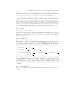
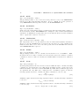
The ENERGYDQMC.dat-file
In this file the time step index ( first column) the mean value of the local energy, hEL i,
(second column), the estimate of the ground state energy, ER , (third column) and the number of random walkers (fourth column) of the Diffusion Quantum Monte Carlo (DQMC)
calculation are printed.
Don’t forget to check the resulting DQMC energy by running the utility program dqmc check.pl.
This program (located at V.32/UTILITYPROGRAMS) takes the ENERGYDQMC.dat-file as input
and checks the correlation between walker populations separated by $m time-steps ( $m = 5
default, and is set by editing the perl script dqmc check.pl). The dqmc check.pl script will
32
CHAPTER 4. SETTING UP A UQANTCHEM CALCULATION
also calculate the mean value of the local energies EL separated by $m time-steps. Remember that uquantchem has no offset when sampling the local energy, EL , i.e $m = 1. Thus
the mean value for the local energy hEL i, given as output directly from uquantchem, might
very well have been calculated over correlated populations.
4.3.13
The DQMCRESTART.dat -file
In this file all the information needed to restart a DQMC calculation is stored. If this
file is present in the running directory of uquantchem, then the DQMC calculation will
be continued from the time-step where the DQMCRESTART.dat -file was most recently updated. Observe that the condition REDISTRIBUTIONFREQ > 0 must be satisfied in order
for the DQMCRESTART.dat to be created. The DQMCRESTART.dat -file is updated every
REDISTRIBUTIONFREQ:th time-step. The possibility to continue a DQMC calculation only
exists for the MPI-version of the code.
4.3.14
The MOLDYNENERGY.dat-file
The energies and temperature are saved to the file: MOLDYNENERGY.dat ,first column = time
step index, second column = total energy, third column = kinetic energy, fourth column =
potential energy, fifth column = temperature and sixth column number of self consistent
cycles performed.
4.3.15
The MOLDYNRESTART.dat-file
In this file contains the information needed to continue a Molecular Dynamics Calculation.
The file contains the following information: 1-st line of file contains the time step index
(integer), the following NATOMS lines contain three columns with the atomic positions corresponding to the time-step index of the first line, the NATOMS lines following the atomic positions contain three columns with the velocities of the atoms corresponding to the time-step
index of the first line, finally the last NATOMS lines contain three colums with the interatomic
forces of the atoms corresponding to the time-step index of the first line. IF THE FILE
MOLDYNRESTART.dat EXISTS IN THE RUNNING DIRECTORY OF UQUANTCHEM
THE CALCULATION WILL BE AUTOMATICALLY CONTINUED. TO RESTART A
MOLECULAR DYNAMICS CALCULATION FROM SCRATCH BE SURE TO REMOVE
THIS FILE FROM THE RUNNING DIRECTORY.
4.3.16
The MOLDYNMOVIE.xsf-file
This file contains atomic positions, in [Å], sampled from a Molecular Dynamics Calculation
and can be used by the xcrysden program to create a gif-movie of the motion of the molecule.
To do this just: >>xcrysden --xsf MOLDYNMOVIE.xsf, then once xcrysden starts the rest
is pretty self explanatory. The resulting movie is most easily viewed by any web browser.
4.3.17
The ATOMPOSITIONS.dat-file
This file contains the latest update of the atomic positions during and after a structural
relaxation calculation.
4.3. THE OUTPUT FILES
4.3.18
33
The HOMO.xsf-file and the LUMO.xsf-file
Contain the HOMO and LUMO orbital values printed on a 3D mesh, and can be used by
the xcrysden program to plot iso surfaces of the respective orbitals.
Chapter 5
Example Calculations
In the sub-directories V.32/EXAMPLE INPUT OUTPUT/ one can find the results of different
uquantchem calculations.
RUN1: contains the output and input of a URHF calculation of a water molecule using a 6 − 31G∗∗ basis set.
RUN2: contains the output and input of a MP2 calculation of a He atom using a ccpVQZ basis set.
RUN3: contains the output and input of a CISD calculation of a H2 molecule atom using
a cc-pVDZ basis set.
RUN4: contains the output and input of a VMC calculation of a H2 molecule atom using
a 6 − 31G∗∗ basis set.
RUN5: contains the output and input of a DQMC calculation of a H2 molecule atom
using a 6 − 31G∗∗ basis set.
RUN6: contains the output and input of a DQMC calculation of a He atom using a
cc-pVTZ basis set.
RUN7: contains the output and input of a RHF charge density calculation for a H2 O
molecule using a 6 − 31G∗∗ basis set.
RUN8: contains the output and input of a RHF of a Cr atom using a 6 − 31∗∗ basis
set. Here the one of the d-orbitals is plotted in the z=0 plane.
RUN9: contains the output and input of a DQMC calculation of a He atom using a
cc-pVTZ basis set. Here the calculation is done with a slightly smaller time step than in
RUN6. Also the charge density has been accumulated from the walker configurations at the
different time steps.
34
35
RUN10: contains the output and input of a VMC calculation of a H2 O using a 6 − 31G∗∗
basis set. Also, the charge density has been calculated from the generated Metropolis configurations.
RUN11-20 I have forgotten the exact type of calculations performed, but I think most
of them are DQMC or VMC calculations.
RUN21: contains the output and input of a structure relaxation calculation for CH4 using
URHF and a 3-21G basis set .
RUN22,26: contains the output and input of a structure relaxation calculation for H2 O
using URHF and a 6 − 31G∗∗ basis set .
RUN27: contains the output and input of a structure relaxation calculation for H2 using URHF and a cc-pVDZ basis set .
RUN31: contains the output and input of a structure relaxation calculation for H2 O using
the PBE functional and a cc-pVTZ basis set .
RUN31: contains the output and input of a structure relaxation calculation for H2 O using
the B3LYP functional and a STO-3G basis set .
RUN33X, RUN33Y, RUN33Z: contains the output and input three TDDFT calculations for H2 O using the PBE functional and the 6-31G basis set . See figure 5.1 for the
resulting absorption spectrum.
36
CHAPTER 5. EXAMPLE CALCULATIONS
1.25
1
H2O (PBE/6-31G)
S(ω)
δt = 0.05 a.u.
0.75
0.5
0.25
0
0
5
10
ω [eV]
15
20
25
Figure 5.1: Absorption spectrum calculated with uquantchem’s TDDFT implementation. Here
3 Dirac pulses where used to produce the spectrum. A 6-31G basis set together with the PBE
functional was used.The corresponding input files are INPUTFILE.RUN33X, INPUTFILE.RUN33Y
and INPUTFILE.RUN33Z. The time step used was 0.05 a.u.
Chapter 6
Utility Matlab programs for
plotting
In the sub-directory V.32/UTILITYPROGRAMS there are a couple of simple matlab scripts that
can help you visualize charge-densities and atomic orbitals calculated with UQUANTCHEM.
37
Chapter 7
For the developer
In this chapter the different subdirectories of the directory V.32/ and their respective content
will be briefly discussed.
7.1
File-map
The following subdirectories are included in the V.32 package:
7.1.1
BASIS
This directory contains the files of all the different gaussian basis-sets that accompany this
release of uquantchem.
7.1.2
BLAS
This directory contains the basic linear algebra sub-programs (BLAS) attached to this release
of uquantchem to enable the compilation of the code in the event that there is no native
BLAS on the machine at which uquantchem is to be installed.
7.1.3
lapack-3.4.0
This directory contains the linear algebra package (LAPACK) attached to this release of
uquantchem to enable the compilation of the code in the event that there is no native
LAPACK on the machine at which uquantchem is to be installed.
7.1.4
UTILITYPROGRAMS
This directory contains a number of utility scripts written in perl or to be used with matlab.
Here follows a list of the included programs and a short description of how the are utilized:
velautocorr.pl
This script takes the uquantchem movie-file: MOLDYNMOVIE.xsf and calculates the velocityauto-correlation function. The result is saved in the file: VELAUTO.dat and performs the temporal fouriertransform of the very same function and saves it to the files SPECTRUM THz.dat
38
7.1. FILE-MAP
39
and SPECTRUM cm.dat
velautocorr2.pl
A slightly modified version of velautocorr.pl.
pdbtoau.pl
For converting the atomic coordinates in pdb-files to a coordinate file suitable for the
uquantchem code.
dqmc check.pl
Calculates the mean local energy EL by using every the local energy at every m:th (integer specified by user inside of script) time-step from the out-put file of a dqmc calculation
ENERGYDQMC.dat. It also calculates the correlation function.
distance.pl
This script takes the uquantchem movie-file: MOLDYNMOVIE.xsf and calculates the interatomic distance between atom A and B as a function of time.
isodens.m
This matlab script uses the out-put file CHARGEDENS.dat to calculate and plot an iso-density
surface of the charge density.
isohomolumo.m
This matlab script uses the out-put files LUMODENS.dat and HOMODENS.dat to calculate and
plot an iso-density surface corresponding to the LUMO and HOMO orbitals.
7.1.5
TESTS
This subdirectory contains the subdirectories: RUN1, RUN2, . . . ,RUN7 which in turn contains
input and output files of seven different test calculations performed with the openmp version
of the uquantchem code. A more detailed specification of these test calculations can be found
in the README-file.
7.1.6
README
This file contains basic information on how to compile the uquantchem code and information
on the different test calculations located in the subdirectory TESTS.
7.1.7
manual.pdf
This manual that you are now reading.
7.1.8
SERIALVERSION
This subdirectory contains all the fortran source files (*.f90) of the serial version of the
uquantchem code together with different Makefiles. Here follows a complete list of the different fortran source files and a short description:
40
CHAPTER 7. FOR THE DEVELOPER
uquantchem.f90
Main program.
datatypemodule.f90
Module in which the different datatypes specific to the uquantchem code have been defined.
exchcorrmodule.f90
Module in which the different exchange correlation functionals have been defined in terms
of subroutines and functions.
random.f90
Module for different random number generators to be used in the diffusion quantum monte
Carlo calculations.
Afunc.f90
This is the function A lri(l1,l2,Ax,Bx,Cx,gamma) defined at the top of page 245 in the Cook
Book.[5]
RHF.f90
Subroutine for performing restricted Hartree Fock calculations.
Fnurec.f90
This subroutine calculates the values F nu(X) (see Cook Book p.280 ) [5] for nu=0,1,2,...,NUMAX,
Through the recursion formula given on the bottom of p. 280 of the Cook Book.
Fnu.f90
The function F nu(x) described in the Cook Book [5] on pages 244 and 280, is here calculated from the Kummer confluent hypergeometric function. See WIRE’s Computational
Molecular Science, 2012, 2: 290-303
CISD.f90
Subroutine for the construction and diagonalization of the configuration interaction Hamiltonian constructed from singles and doubles excitations.
getK.f90
Subroutine calculating the the exchange matrix Kil by contracting the electron-electron integrals (ij|kl) with the density matrix Pjk .
getKv.f90
Vectorized version of getK.f90.
getJ.f90
Subroutine calculating the the Hartree matrix Jij by contracting the electron-electron integrals (ij|kl) with the density matrix Pkl .
getJv.f90
Vectorized version of getJ.f90.
7.1. FILE-MAP
41
gammaf.f90
calculates the value of the GAMMA-function Γ(I + 0.5) gfortan has the gamma function as
an intrinsic function whereas ifort on osx does not seem to have it.
fj.f90
The function f j(l,m,a,b) on page 237 in the Cook book [5].
fac.f90
simple factorial function: n!
gto.f90
Calculates the value at argument for a spherically symmetric gto basis function consisting
of contracted primitive gaussians.
gtop.f90
Calculates the radial derivative, at argument r, of a spherically symmetric gto basis function
consisting of contracted primitive gaussians.
gtopp.f90
Calculates the second radial derivative, at argument r, of a spherically symmetric gto basis
function consisting of contracted primitive gaussians.
gtoppp.f90
Calculates the third radial derivative, at argument r, of a spherically symmetric gto basis
function consisting of contracted primitive gaussians.
eeints.f90
Subroutine that calculates the electron-electron integrals (ij|kl) by Rys quadrature.
diaghHF.f90
Subroutine that calculates the eigenvalues, , and eigenvectors, C, to the eigenvalue problem: F C = SC. Here, F , corresponds to the Fockian matrix and S the overlap matrix.
diagh.f90
Subroutine that calculates the eigenvalues, , and eigenvectors, C, to the eigenvalue problem: HC = C. Here, H, typically corresponds to the Hamiltonian matrix.
dfac.f90
Function that calculates the double factorial, n!!.
checkinputfile.f90
This subroutine checks wheater or not the file ’INPUTFILE’ exists and if so, how many
lines, NLINES, it contains before the entry of the number of atoms, NATOMS.
chargedenssave.f90
This subroutine calculates and saves the charge-density on disk.
42
CHAPTER 7. FOR THE DEVELOPER
exciteornot.f90
Function used to decide which excitations to use when performing a CISD calculation.
hforbitalsave.f90
Subroutine that calculates the values of a Hartree-Fock or Kohn-sham orbital on a mesh
and saves the result to disk.
binomfac.f90
calculates the binomial factor
N
M
=
N!
M !(N −M )!
basfunkval.f90
Calculates the value of a real basis-function, ψi , at the spatial point r ∈ R3 . I.e, ψi (r).
URHF.f90
Subroutine for performing unrestricted Hartree Fock calculations.
primeeintegral.f90
Function that calculates the electron repulsion integrals (µν|κλ) over the primitive gaussian
functions φµ , φν , φκ , φλ , i,e:
Z
(µν|κλ) =
d3 r
Z
d3 r0
φµ (r), φν (r), φκ (r0 ), φλ (r0 )
|r − r0 |
potential.f90
Subroutine that calculates the potential matrix, Vij , and the nuclear gradients of the potential matrix, ∇R Vij . Where Vij is defined by
Vij = −
XZ
k
d3 rZk
ψi (r)ψj (r)
.
|r − Rk |
Here, Rk are the positions of the nuclei in the molecule and Zk are the respective atomic
numbers.
overlap.f90
Subroutine that calculates the overlap matrix, Sij , and the nuclear gradients of the overlap
matrix, ∇R Sij . Where Sij is defined by
Z
Sij =
d3 rψi (r)ψj (r).
oneint.f90
This function calculates the Ix(ta) term on p. 974 in J. Comp. Chem. 11, 972-977 (1990)
which is used to calculate the two electron integrals through Rys-quadrature.
7.1. FILE-MAP
43
normalize.f90
This subroutine calculates the normalization constants for all of the basis functions.
ROOTWEIGHT5.f90
Subroutine that calculates the roots and weights of 5:th order Rys polynomials. The calculation is done by polynomial fits of pree-calculated roots and weights. The fits are taken
from the GAMES-package ( Same as in Pyquante), a very fast process.
leastsq.f90
Performs a least square fit of the function f (r) = Ae−λr + C to the N data points r(i) =
rc
y(i) = GT O(r(i)), i = 1, 2, . . . , N
N −1 ∗ (i − 1),
makedens.f90
Subroutine that calculates the density matrix, Pµν , from the eigen-vectors of the Fockian/KhonSham Hamiltonian, Ci , i.e
N
occ
X
†
Cµi Cνi
Pµν =
i=1
kinetic.f90
Subroutine that calculates the Kinetic energy matrix, Tij , and the nuclear gradients of the
kinetic energy matrix, ∇R Tij . Where Sij is defined by
1
Tij = −
2
Z
d3 rψi (r)∇2 ψj (r).
ijkl.f90
Function that contacts the 4-component index i,j,k,l, used to label the different electronelectron repulsion integrals (ij|kl), into one single index.
homolumosave.f90
Subroutine that calculates the densities and orbital values of the HOMO and LUMO orbitals
on a mesh and writes the result to the files HOMODENS.dat, LUMODENS.dat, HOMO.xsf and
LUMO.xsf.
gettotalbasis.f90
If the logical input variable COUNTER=.TRUE. , this subroutine calculates the size of the
total basis set from the local basis sets centered at the different atoms If COUNTER=.FALSE.
, this subroutine returns the total basis set.
rysquad.f
This subroutine calculates the roots and weights of a Rys polynomial of arbitrary order.
44
CHAPTER 7. FOR THE DEVELOPER
rho.f90
Function that calculates the charge density, ρ, from the basis functions and the density
matrix P at one point in space.
readin.f90
Subroutine that reads the user specified data stored in the file INPUTFILE.
ROOTWEIGHT4.f90
Subroutine that calculates the roots and weights of 4:th order Rys polynomials. The calculation is done by polynomial fits of pree-calculated roots and weights. The fits are taken
from the GAMES-package ( Same as in Pyquante), a very fast process.
interpol.f90
This routine calculates the interpolating cubic polynomial linking together the second derivative of an sto-type basis function: sto00 (r) = Aλ2 e−λr at the point r = rc , and a the second
derivative of a gto-type basis function: gto00 (r) at r = rc + δr so that both the second and
the third derivative of the polynomial matches that sto at r = rc and the gto at r = rc + δr.
This is done according to J. Chem. Phys. 115, 5362 (2001).
gradbasfunkval.f90
Subroutine that calculates the gradient of a real basis-function, φµ , at the spatial point
r ∈ R3 . I.e, the gradient = ∇φµ (r).
laplacebasfunkval.f90
Function that calculates the value of the laplacian of a real basis-function, φµ , at the spatial
point r ∈ R3 . I.e, the laplacian = ∇2 φµ (r).
hforbitalval.f90
Function that calculates the value of a Hartree-Fock orbital or a Kohn-Sham orbital at the
spatial point r ∈ R3 , given the eigen-vector Ci . I.e the value Ψi (r).
gradhforbitalval.f90
Subroutine that calculates the gradient of a Hartree-Fock orbital or a Kohn-Sham orbital
at the spatial point r ∈ R3 , given the eigen-vector Ci . I.e the gradient = ∇Ψi (r).
laplacehforbitalval.f90
Subroutine that calculates the laplacian of a Hartree-Fock orbital or a Kohn-Sham orbital
at the spatial point r ∈ R3 , given the eigen-vector Ci . I.e the laplacian = ∇2 Ψi (r).
det.f90
This function calculates the determinant of a NxN matrix A, by first transforming it into
upper diagonal form.
7.1. FILE-MAP
45
stoexponent.f90
Finds the exponent, λ, and coeficient, A, of a slater type orbital, Ae−λr by fiting it
to the gaussian basis function, gto(r), at the inflexion point rc , i.e at the point where
gto0 (rc ) = min. The exponent, λ, and coeficient, A are calculated from the continuity conditions:
(1) gto(rc ) = Ae−λrc
(2) gto0 (rc ) = −Aλe−λrc
0
leading to λ = −gto0 (rc )/gto(rc ), and A = gto(rc )e−gto (rc )rc /gto(rc )
slaterdet.f90
This fuction calculates the slater determiant from:
(a) N = Total Number of electrons,
(b) BAS = Hartree Fock basis
(c) C = Fockian eigenvectors,
(d) r = positions the electrons 3N-long array
(e) UP = .TRUE. Spin up slater determinant is calculated, otherwise spin-down slater determinant is to be calculated.
(f) NS = slater determinant dimension.
gradslaterdet.f90
This subroutine calculates the gradient of a slater determiant, with respect to the electron
coordinate I, from:
(a) N = Total Number of electrons,
(b) BAS = Hartree Fock basis
(c) C = Fockian eigenvectors,
(d) r = positions the electrons 3N-long array
(e) UP = .TRUE. if I = spin upp orbital, else UP = .FALSE.
(f) NS = Slaterdeterminant dimension
laplaceslaterdet.f90
This fuction calculates the laplacian of a slater determiant, with respect to the electron
coordinate I, from:
(a) N = Total Number of electrons,
(b) BAS = Hartree Fock basis
(c) C = Fockian eigenvectors,
(d) r = positions the electrons 3N-long array
(e) NS = Slaterdeterminant dimension.
(f) UP = .TRUE. if I = spin upp orbital, else UP = .FALSE.
jastrowup.f90
This function calculates the Jastrow factor contribution from the spin-up electrons. N =
total number of electrons r = coordinates of all electrons, r is a 3*N-long array b,c = jastrow
parameters.
46
CHAPTER 7. FOR THE DEVELOPER
jastrowdown.f90
This function calculates the Jastrow factor contribution from the spin-down electrons. N =
total number of electrons r = coordinates of all electrons, r is a 3*N-long array b,c = jastrow
parameters.
jastrowud.f90
This function calculates the Jastrow factor contribution from the cross-terms between spinup and spin-down electrons. N = total number of electrons r = coordinates of all electrons,
r is a 3*N long-array b,c = jastrow parameters.
jastrow.f90
This function calculates the (Total) Jastrow factor. N = total number of electrons r =
coordinates of all electrons, r is a 3*N-long array b,c = jastrow parameters.
DIIS.f90
This is the direct inversion in the iterative subspace method DIIS, by P. Puley in CHEM.
Phys. Lett. 73, 393 (1984). The routine is used to estimate the self-consistent densitymatrix in the region where the density dependence of the energy can be approximated well
up to second order. Also, see T. Halgaker, P. Jorgensen and J. Olsen ”Molecular Electronic
Structure Theory” p.460-463
findclosestatom.f90
Subroutine that finds the atomic nucleus located closest to a particular electron. The motivation for the use of this routine can be found in J. Chem. Phys. 99 , 2865-2890, (1993).
gradjastrow.f90
This subroutine calculates the gradient of the Jastrow factor, with respect to the electron
coordinate I.
N = total number of electrons
r = coordinates of all electrons, r is a 3*N-long array
b,c = jastrow parameters.
laplacejastrow.f90
This function calculates the laplacian of the Jastrow factor, with respect to the electron
coordinate I.
N = total number of electrons
r = coordinates of all electrons, r is a Nx3-array
b,c = jastrow parameters.
guideforce.f90
This subroutine calculates the guiding force used in the DQMC importance sampling.
trialfnk.f90
This function calculates the value of the trial function, used in the DQMC importance
sampling, at a specific point in the 3Ne dimensional coordinate space of the electrons.
(Ne =number of electrons)
7.1. FILE-MAP
47
laplacetrialfnk.f90
This function calculates the value of laplacian of the trial function, used in the DQMC
importance sampling, at a specific point in the 3Ne dimensional coordinate space of the
electrons. (Ne =number of electrons)
EL.f90
This function calculates the Local energy of the trial function, at a specific point in the
3Ne dimensional coordinate space of the electrons (Ne =number of electrons). Used in the
DQMC importance sampling.
dqmc.f90
This routine performs the diffusion quantum Monte Carlo or the Variational Quantum Monte
Carlo calculations. This is the routine that is at the top of the hierarchy/program-tree, i.e
the control routine, of all the quantum Monte Carlo calculations.
preparedifusion.f90
Subroutine that performs a series of calculations in order to enable a diffusion step in the
DQMC calculation. For details see J. Chem. Phys. 99 , 2865-2890, (1993), and the comments embedded in the source of this routine.
ROOTWEIGHTMAX3.f90
Subroutine that calculates the roots and weights of Rys polynomials of order ≤ 3. The calculation is done by polynomial fits of pree-calculated roots and weights. The fits are taken
from the GAMES-package ( Same as in Pyquante), a very fast process.
readbasis.f90
This subroutine reads in the expansion coefficients and exponents of the gaussian basis-set
stored in the file BASISFILE.
primpotential.f90
This function calculates the potential energy integral given on the bottom of p. 244 in the
Cook Book [5].
primoverlap.f90
This function calculates the overlap integral S = Sx Sy Sz as given by the expressions on the
pages 234-238 in the Cook book [5].
primkinetic.f90
This function returns the integral hGT O1 |− 12 ∇2 |GT O2 i as given by the cook Book on pages
234-239 [5]. Here GT Oi are primitive gaussian functions.
MP2.f90
Subroutine that performs second order Møller-Plesset calculations.
gradprimoverlap.f90
This subroutine calculates the nuclear gradients of the overlap integral S = Sx Sy Sz as given
by the expressions on the pages 234-238 in the Cook book [5].
48
CHAPTER 7. FOR THE DEVELOPER
gradprimkinetic.f90
This subroutine calculates the nuclear gradients of the integral hGT O1 | − 12 ∇2 |GT O2 i as
given by the cook Book on pages 234-239 [5]. Here GT Oi are primitive gaussian functions.
gradprimpotential.f90
This subroutine calculates the nuclear gradients of the potential energy integral given on
the bottom of p. 244 in the Cook Book [5].
gradprimeeintegral.f90
This subroutine calculates the nuclear gradients of the two-electron integral between primitive gaussians.
forces.f90
This subroutine calculates the interatomic forces on all atoms of the molecule.
dAfunc.f90
This function calculates the derivative of the function Alri (l1 , l2 , Ax , Bx , Cx , γ) ( defined at
the top of page 245 in the Cook Book [5]) with respect to Cx .
relax.f90
This subroutine calculates the atomic positions of the molecule that corresponds to the minimal energy.
linesearchmin.f90
This subroutine fits a number of NPOINTS energies and moves to 4:th order polynomial in
the interval [0, DR] and calculates the position of the minimum of this polynomial in the
interval [0, DR]. This routine is used by relax.f90 in order to find the move involved a
steepest decent or a conjugate gradient calculation.
massa.f90
This function just give the atomic mass as output given the atomic number as input. The
atomic masses have been taken from Aschcroft and Mermins ”Solid State Physics”.
moleculardynamics.f90
Subroutine that performs molecular dynamics calculations.
moleculardynamicssoft.f90
Subroutine that performs molecular dynamics calculations, with a so called soft-start. See,
the description of the input parameter SOFTSTART.
invert.f90
Subroutine that inverts a N × N real matrix.
vxc.f90
This subroutine calculates the exchange correlation potential.
7.1. FILE-MAP
49
vxcalt.f90
Subroutine not used for the moment.
dvxc.f90
Subroutine not used for the moment.
ngbasfunkval.f90
Calculates the value of the gradient of a real basis-function at the spatial point r ∈ R3 , with
respect to the nuclear coordinates at which the basis function is centered.
nggradbasfunkval
Calculates the value of nuclear gradient of the gradient of a real basis-function, Ψ, at the
spatial point r = (x, y, z). I.e, the elements of the tensor = ∇R [∇Ψ(r)]. The output is
stored in the 3x3 matrix nggrad, according to the following ordering:
nggrad(1, 1) =
nggrad(2, 1) =
nggrad(3, 1) =
∂2Ψ
∂Rx ∂x ,
∂2Ψ
∂Rx ∂y ,
∂2Ψ
∂Rx ∂z ,
nggrad(1, 2) =
nggrad(2, 2) =
nggrad(3, 2) =
∂2Ψ
∂Ry ∂x ,
∂2Ψ
∂Ry ∂y ,
∂2Ψ
∂Ry ∂z ,
nggrad(1, 3) =
nggrad(2, 3) =
nggrad(3, 3) =
∂2Ψ
∂Rz ∂x
∂2Ψ
∂Rz ∂y
∂2Ψ
∂Rz ∂z
nglaplacebasfunkval.f90
Calculates the value of nuclear gradient of the laplacian of a real basis-function at the spatial
point r ∈ R3 . I.e, The function = ∇R [∇2 Ψ(r)] The output is stored in the array, nglapl,
according to the following ordering:
nglapl(1) = d∇2 Ψ(r)/dRx
nglapl(2) = d∇2 Ψ(r)/dRy
nglapl(3) = d∇2 Ψ(r)/dRz
getvxcr.f90
This subroutine calculate the r-dependent matrix elements Φi (r)Vxc (r)Φj (r) and the nuclear gradient of these matrix elements. After integration over the entire 3-DIM space with
some quadrature these will become the exchange correlation potential matrix elements to
be plugged into the Kohn-sham hamiltonian, and the corresponding force expression for the
exchange correlation contribution to the interatomic forces.
atomicradii.f90
This function takes the atomic number as input and returns the empirical radii of Bragg
and Slater, J. C. Slater, J. Chem. Phys. 41, 3199 (1964).
lebedev.f90
This subroutine provides the weights and roots of the Lebedev quadrature used for the integration on the surface of a sphere.
chebgauss.f90
This subroutine calculates the weights and roots of the Chebyshev-Gauss quadrature of the
second kind used for the integration along the radial direction.
50
CHAPTER 7. FOR THE DEVELOPER
sofmu.f90
This is the function s(µ) = 12 (1 − f (µ)) described by Eqn (3) in A. D. Becke, J. Chem. Phys.
88, 2547 (1988). Here the recommended third order (k=3) is used.
pvoronoi.f90
This function is given by Eqn. (13) in A. D. Becke, J. Chem. Phys. 88, 2547 (1988).
getvxc.f90
This subroutine calculates the exchange correlation potential matrix elements, hi|Vxc |ji,
and the nuclear gradients of these matrix elements, ∇R hi|Vxc |ji, using the resolution of the
identity into fuzzy polyheadra prescribed by A. D. Becke, J. Chem. Phys. 88, 2547 (1988),
together with Gauss-Chebysshev and Lebedev quadrature.
excdens.f90
This function calculates the exchange correlation energy density.
excdr.f90
This function calculates the exchange correlation energy density.
exc.f90
This function calculates the exchange correlation energy from the exchange correlation energy density by using the resolution of the identity into fuzzy polyheadra prescribed by A.
D. Becke, J. Chem. Phys. 88, 2547 (1988), together with Gauss-Chebysshev and Lebedev
quadrature.
DFT.f90
Subroutine performing density functional theory calculations.
quadcheck.f90
Calculates the total number of electrons by integrating the charge density, ρ(r) by using the
resolution of the identity into fuzzy polyheadra prescribed by A. D. Becke, J. Chem. Phys.
88, 2547 (1988), together with Gauss-Chebysshev and Lebedev quadrature. This is used to
check the quality of the quadrature mesh.
TRACE.f90
Calculates the trace of a square matrix.
hessianbasfunk.f90
Calculates the hessian of a real basis-function, Ψ, at the spatial point r ∈ R3 . I.e, the matrix
2
Ψ
hij = ∂x∂i ∂x
j
hessianrho.f90
This subroutine calculates the hessian matrix of the charge density, ρ(r), i.e:
∂2ρ
hi,j,k = ∂R(k)
where R(k)i = i:th coordinate of the nucleus positioned at R(k) and rj =
i ∂rj
the j:th coordinate of the spatial electron coordinate r.
7.1. FILE-MAP
51
dftforcedens.f90
This subroutine calculates the exchange correlation force density at the point r ∈ R3 in
space.
getxcforce.f90
This subroutine calculates the exchange correlation contribution to the interatomic forces
by integration of the exchange correlation force density. This is done by using the resolution
of the identity into fuzzy polyheadra prescribed by A. D. Becke, J. Chem. Phys. 88, 2547
(1988), together with Gauss-Chebysshev and Lebedev quadrature.
pnonorm.f90
This function is given by Eqn. (13) in A. D. Becke, J. Chem. Phys. 88, 2547 (1988).
tmu.f90
This function is the function t(µ) described in appendix B Eqn (B9) In J. Chem. Phys. 98,
5612, (1993),
gradpvoronoi.f90
This subroutine calculates all the nuclear gradients of the Becke weight function centered
at atom I. See Appendix B in J. Chem. Phys. 98, 5612 (1993).
gradoverlap.f90
Here we calculate the gradient of the overlap matrix when all the basis functions have been
shifted with the vector r → R + r, i.e Φ(r) → Φ(r + R).
relaxf.f90
This subroutine searches for the atomic positions at which all nuclear forces are < FTOL.
mulliken.f90
Subroutine that calculates the Mulliken charges of the different atoms and prints the result
in the stout.
7.1.9
OPENMPVERSION
This subdirectory contains all the fortran source files (*.f90) of the opemp version of the
uquantchem code together with different Makefiles. The source files within this directory
have the same names and functionality as the *.f90 files located in the SERIALVERSION directory. For a complete listing of the fortran source files contained in the OPENMPVERSIONdirectory se the preceding subsection.
7.1.10
MPI VERSION
This subdirectory contains all the fortran source files (*.f90) of the mpi version of the
uquantchem code together with different Makefiles. The source files within this directory
have the same names and functionality as the *.f90 files located in the SERIALVERSION directory. For a listing of the fortran source files contained in the MPI VERSION-directory se
the above section describing the SERIALVERSION. However, there are a couple of source files
52
CHAPTER 7. FOR THE DEVELOPER
in the MPI VERSION-directory that are unique to the mpi-version of the code. Below follow
a complete listing of these files:
diagscalapack.f90
Subroutine that uses the ScaLapack routine PDSYEVD to diagonalize the CISD hamiltonian matrix by the divide and conquer algorithm.
gridsetup.f90
This subroutine factorizes the number of processors (nproc) into nprow and npcol, that are
the sizes of the 2-d processors mesh.
countee.f90
Calculates the diagonal electron-electron integrals (ij|ij) and counts the number of integrals
that give a considerable contribution to the exchange and Hartree matrices Kij and Jij .
Here we use the Schwartz inequality |(i, j, k, l)| ≤ [|(i, j, i, j)(k, l, k, l)]1/2 (See Eqn 9.12.25
p.404 in T. Helgaker et al’s ”Molecular Electronic-Structure Theory” ) together with Eqn.
(56) and (57) page. 86, in Haettig, ”Multiscale Simulation Methods in Molecular Sciences”
, J. Grotendorst, N. Attig, S. Blugel, D. Marx (Eds.), Institute for Advanced Simulation,
Forschungszentrum Julich, NIC Series, Vol. 42, ISBN 978-3-9810843-8-2,pp. 77-120, 2009,
to decide wich integrals give considerable contributions.
Bibliography
[1] S. H. Vosko, L. Wilk and M. Nusair, Can. J. Phys. 58, 1200 (1980).
[2] John P. Perdew, Kieron Burke, Matthias Ernzerhof, Phys. Rev. Lett, 77, 3865 (1996)
[3] A. Szabo and N. S. Ostlund, Modern Quantum Chemistry, Dover, Mineola, New York
(1996)
[4] X. Li, S. M. Smith, A. N. Markevitch, D. A. Romanov, R. J. Lewis and H. B. Schlegel,
Phys. Chem. Chem. Phys. 7, 233 (2005)
[5] D. B. Cook, Handbook of Computational Chemistry, Dover, Mineola, New York (2005)
[6] J. M. Thijssen, Computational Physics, Page 330. (Cambridge)
[7] P. Puley, Chem. Phys. Lett. 73, 393 (1980)
[8] P. Puley, J. Comp. Chem., 3, 556 (1982).
[9] S. E Koonin and D. C. Meredith, Computational Physics, Page 213-214, (West wide
Press 1990)
[10] C. J. Umrigar, M. P. Nightingale, K. J. Runge, J. Chem. Phys. 99, 2865 (1993)
[11] S. Manten and A. Lüchow, J.Chem.Phys. 115, 5362 (2001)
[12] A. M. N. Niklasson, C. J. Tymczak, and M. Challacombe, Phys. Rev. Lett. 100, 123004
(2008); Phys. Rev. Lett. 97, 123001 (2006)
[13] J. A Pople, R. Krishnan, H. B. Schlegel and J. S. Binkley Int. J. Quantum Chemistry:
Quantum Chemistry Symposium 13, 225-241, see eqn (21) p. 229
[14] H. Bernhard Schlegel, Theor. Chem. Acc. 103, 294-296, here see eqn 3-7
[15] Anders M. N. Niklasson and Marc J. Cawkwell , Phys. Rev. B 86, 174308 (2012)
[16] Anders M. N. Niklasson, Peter Steneteg,Anders Odell, Nicolas Bock, Matt Challacombe,
C. J. Tymczak, Erik Holmstrm, Guishan Zheng and Valery Weber, J. Chem. Phys. 130
, 214109 (2009)
[17] B. Mielich, A. Savin, H. Stoll and H. Preuss, Chem. Phys. Lett. 157, 200 (1989)
[18] A. D. Becke, Phys. Rev. A, bf 38, 3098 (1988)
53
54
BIBLIOGRAPHY
[19] P. J. Stephens, F. J. Devlin, C. F. Chabalowski and M. J. Frisch J. Phys. Chem bf 98
11623 (1994)
[20] B. G. Johnsonm P. M. W. Gill and J. A. Pople, J. Chem Phys. 98 5612 (1993)