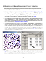
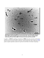
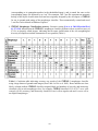
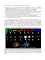
Download CMEIAS Ver. 1.28 - The Center for Microbial Ecology

©
CMEIAS Ver. 1.28
User Manual
Custom Plug-ins operating in UTHSCSA ImageTool Ver. 1.28
Advanced Image Analysis Software Designed to
Strengthen Microscopy-Based Approaches
for Understanding Microbial Ecology
F. B. Dazzo, D. Trione, E. Marshall & J. Zurdo
Center for Microbial Ecology, Michigan State University,
East Lansing, MI 48824 USA
CMEIAS© is copyrighted by Michigan State University. All rights reserved.
-1-
Table of Contents
CMEIAS© License Agreement [Michigan State University]…………………………………... 5
UTHSCSA ImageTool© License Agreement .……………………………..…………….………. 6
Background Reading, Acknowledgments, About CMEIAS Shield ...……………..….…….. 7
1 INTRODUCTION & NEW FEATURES…….…….………………………………………………. 8
2 REQUIREMENTS, DOWNLOAD and INSTALLATION……………..……………..………… 11
2.1 System Requirements……………………………………………………………………………. 11
2.2 Download & Installation of ImageTool/CMEIAS ver. 1.28 …………………...………… 12
3 MICROBIAL SAMPLE PREPARATION, MICROSCOPY & IMAGE PREPARATION…… 13
3.1 Image Requirements for Image Analysis……….…………………………………………... 13
3.2 Preparation of Agarose-Coated Slides……………...……………….………………..……. 14
3.3 Preparation of Dispersed Microbial Samples…………………………………...………… 15
3.4 Phase-Contrast Microscopy of Refractile, Immobilized Cells…….………………….. 15
3.5 Image Acquisition & Sampling Density…….……………………………………………….. 16
3.6 Image Size and Pixel Resolution……………………………...……………………..……….. 17
3.7 Image Editing…………………………………………………………………..……………….……. 18
3.8 Adding a Calibrated Bar Scale……………………………………………..……...…………... 20
4 SETTING PREFERENCES PRIOR to IMAGE ANALYSIS…….……………………………. 21
4.1 Measurement Features Used in Object Analysis…………..…..……….………………... 21
4.1.1
4.1.2
4.1.3
4.1.4
Measurement features preference page………………….………………………….….………... 21
Definitions of measurement features for object analysis……………………………...……… 22
Measurement Precision (decimal places)………………………………………………………… 26
Display of object analysis data in the Results Window……………………………………….. 27
4.2 Find Objects Settings.……………………………………………………..……..….…………… 28
4.2.1
Area of Interest (AOI) Options………………………………………………………..….…………. 28
4.2.1.1. Search entire image………………………………………………………………………… 28
4.2.1.2. Search in AOI (Area of Interest)......................…………….……………………………. 28
4.2.2
Search options………………………………………………………………………………………… 29
4.2.2.1 Manually select objects……………………………………………….………..….………. 29
4.2.2.2 Automatically select objects………….……………………………….………..…………. 29
4.2.2.3 Include objects at edge of image…………………………………..…………..…………. 29
4.2.2.4 Exclude background………………………………………………….………..…….……… 29
-2-
4.2.2.5 Maximum # of objects………………………………………………...….………..………... 29
4.2.2.6 Minimum object size (pixels)……………………………………..…...…………………… 30
4.2.3
Display Options……………………………………………………………………………………….. 31
4.2.3.1 Show object count in a message box……………………………………………………. 31
4.2.3.2 Place object count in Results window…………………………….……………………. 31
4.2.3.3 Concatenate Object Analysis results……………………………………………………. 31
4.2.3.4 Show object numbers on original image………………………………………………… 32
4.2.3.5 Choose font…………………………………………………………………………..…….… 33
4.2.3.6 Show object outlines on original image………………………………………….……… 33
4.2.3.7 Choose color…………………………………………………………………………………. 33
4.3
Image Settings………………………………………………………………..………………... 34
4.3.1
4.3.2
4.3.3
4.3.4
Origin of X, Y Cartesian coordinate system in image windows……………..………………..34
Prompt to save untitled images…………………………………………………………………… 34
Show full path names in image title bars………………………………………………………… 34
Initial zoom/scale factor……………………………………………………………………………… 34
5 IMAGE DISPLAY ADJUSTMENTS, CALIBRATION, and THRESHOLDING…...….…… 35
5.1 Load Image………………………………………………………………………………….………. 35
5.2 Adjust Image Size…………………………………………………………………………………. 35
5.3 Image Transformations………………………………………………………………………….. 36
5.4 Adjust Image Contrast / Brightness………………………………………………………….. 36
5.5 Negative Image Transformation……………………………………………………….…….… 37
5.6 Spatially Calibrate the Image …...………………………………………………………………. 38
5.7 Find Objects by Brightness Threshold Segmentation …………….………………….. 40
5.7.1
5.7.2
5.7.3
Activate threshold selections…………………………………………………………….……… 40
Find objects in a binary image…………………………………………………..…….…….…….. 41
Find objects in a non-binary image………………………………………………….……………. 42
5.8 Manually Select Objects..………………………………………………………………..……… 44
6 PERFORMING OBJECT ANALYSIS…………………………………………………………. 45
6.1 Overview of Settings, Preferences & Object Segmentation…………………..……… 45
6.2 Object Counting…………………………………………………………………….……………… 45
6.2.1
6.2.2
Automatic Object Counting…………………………………………………………………………. 45
Manual Object Counting……………………………………………………….……………………. 47
6.3 Automatic and Manual Measurement Feature Extraction.……….……………………. 48
6.4 Working with Object Analysis Data in the Results Window…………………………... 50
-3-
7 PERFORMING OBJECT CLASSIFICATION……………………….…………..…………….. 51
7.1 ImageTool/CMEIAS-1D Object Classifier………………………...…………….…………... 52
7.1.1 Using the IT / CMEIAS-1D Object Classifier for cell size classification………………………….53
7.1.2 Using the IT / CMEIAS-1D Object Classifier for cell shape classification………………….……54
7.2 CMEIAS-2 Morphotype Classifier.…………………………………………………………….. 55
7.2.1
7.2.2
7.2.3
7.2.4
7.2.5
7.2.6
Hierarchy of characteristics for CMEIAS microbial morphotype classification…………….... 57
Steps to perform a CMEIAS Morphotype Classification…………………………………………..58
Important points regarding the CMEIAS Morphotype Classifier….………….………………… 59
Sources of morphotype classification error and the CMEIAS edit feature ………………….. 61
Editing the type-1 misclassification error in a CMEIAS Morphotype Classification………. 62
Editing the Type-2 (unrecognized class) and Type-3 (invalid object) classification errors.. 63
8 GRAPHICS and ECOLOGICAL STATISTICS of CMEIAS OBJECT ANALYSIS
& CLASSIFICATION DATA………………………………………………………..……….. 66
APPENDIX I CMEIAS 1.28 Training Tutorial Macro………………………………...……………. I
APPENDIX II CMEIAS Object Analysis Macro…………………………..……….….…………. XIX
APPENDIX III ImageTool/CMEIAS-1D Object Classification Macro………….……..……..XXI
APPENDIX IV CMEIAS-2 Morphotype Classification Macro……………………………..…XXIII
APPENDIX V Known Problems in UTHSCSA ImageTool 1.28………………….………….XXVI
APPENDIX VI Studies using CMEIAS …………………....…………………………………....XXVII
-4-
CMEIAS© Ver. 1.28 (Center for Microbial Ecology Image Analysis System)
Michigan State University Software License Agreement
By downloading and installing a copy of the CMEIAS© Software and Documentation, you agree to the
following terms:
Notification of Copyright: CMEIAS© is a proprietary product of Michigan State University (“MSU”)
and is protected by copyright laws and international treaty. You (as “End User”) must treat CMEIAS
like any other copyrighted materials. Copyright laws prohibit making copies of the Software for any
reason. You may make copies of the Documentation for use with a licensed version of the Software;
however, MSU notifications of copyright must be left intact. If you have any questions concerning this
agreement, please contact the Office of Intellectual Property, MSU, East Lansing, Michigan 48824
U.S.A. (517) 355-2186.
UTHSCSA ImageTool Code: CMEIAS© incorporates source code from ImageTool software developed
by the University of Texas Health Science Center at San Antonio. The ImageTool code contained in
CMEIAS© is a modified version of the code, and not the original UTHSCSA ImageTool distributed by
the University of Texas. The license pertaining to the UTHSCSA code is included in the
download/installation of ImageTool <http://ddsdx.uthscsa.edu/dig/itdesc.html> and this operator
manual, and is binding on you upon your use of the CMEIAS code.
License: MSU grants End User the royalty-free, non-exclusive, non-transferable right to use CMEIAS©
Ver. 1.28 software for research, training or educational purposes. You may not redistribute, transfer,
rent, lease, sell, lend, sub-license, prepare derivative works, decompile, or reverse-engineer the
CMEIAS© Software without prior express written consent of MSU at the above address.
MSU retains title to CMEIAS©, including without limitation the Software and Documentation. End
User agrees to use reasonable efforts to protect the Software and Documentation from unauthorized
use, reproduction, distribution, or publication. All rights not specifically granted in this Agreement are
reserved by MSU.
Warranty: CMEIAS© Software and Documentation are provided “as is.” MSU MAKES NO
WARRANTY, EXPRESS OR IMPLIED, TO END USER OR TO ANY OTHER PERSON OR
ENTITY. SPECIFICALLY, MSU MAKES NO WARRANTY OF MERCHANTABILITY OR
FITNESS FOR A PARTICULAR PURPOSE OF CMEIAS SOFTWARE OR DOCUMENTATION.
MSU WILL NOT BE LIABLE FOR SPECIAL, INCIDENTAL, CONSEQUENTIAL, INDIRECT OR
OTHER SIMILAR DAMAGES, EVEN IF MSU OR ITS EMPLOYEES HAVE BEEN ADVISED OF
THE POSSIBILITY OF SUCH DAMAGES. IN NO EVENT WILL MSU LIABILITY FOR ANY
DAMAGES TO END USER OR ANY PERSON EVER EXCEED THE FEE PAID FOR THE
LICENSE TO USE THE SOFTWARE, REGARDLESS OF THE FORM OF THE CLAIM.
General: If any provision of this Agreement is unlawful, void, or for any reason unenforceable, it shall
be deemed severable from, and shall in no way affect the validity or enforceability of the remaining
provisions of this Agreement. This agreement shall be governed by Michigan law.
-5-
UTHSCSA ImageTool©License Agreement
University of Texas Health Science Center at San Antonio (UTHSCSA, Texas)
UTHSCSA ImageTool software [both binary and source (if released)] (hereafter, Software) is
copyrighted by The Board of Trustees of the University of Texas (UT), and ownership remains with the
UT.
The UT grants you (hereafter, Licensee) a license to use the Software for academic, research and
internal business purposes only, without a fee. Licensee may distribute the binary and source code (if
released) to third parties provided that the copyright notice and this statement appear on all copies and
that no charge is associated with such copies.
Licensee may make derivative works. However, if Licensee distributes any derivative work based on or
derived from the Software, then Licensee will
(1) notify UTHSCSA regarding its distribution of the derivative work, and
(2) clearly notify users that such derivative work is a modified version and not the original UTHSCSA
ImageTool distributed by the UT.
Any Licensee wishing to make commercial use of the Software should contact the UT, c/o UTHSCSA,
to negotiate an appropriate license for such commercial use. Commercial use includes (1) integration of
all or part of the source code into a product for sale or license by or on behalf of Licensee to third
parties, or (2) distribution of the binary code or source code to third parties that need it to utilize a
commercial product sold or licensed by or on behalf of Licensee.
UT MAKES NO REPRESENTATIONS ABOUT THE SUITABILITY OF THIS SOFTWARE FOR
ANY PURPOSE. IT IS PROVIDED "AS IS" WITHOUT EXPRESS OR IMPLIED WARRANTY.
THE UT SHALL NOT BE LIABLE FOR ANY DAMAGES SUFFERED BY THE USERS OF THIS
SOFTWARE.
By using or copying this Software, Licensee agrees to abide by the copyright law and all other
applicable laws of the U.S. including, but not limited to, export control laws, and the terms of this
license. UT shall have the right to terminate this license immediately by written notice upon Licensee's
breach of, or non-compliance with, any of its terms. Licensee may be held legally responsible for any
copyright infringement that is caused or encouraged by Licensee's failure to abide by the terms of this
license.
For more information contact <[email protected]>.
-6-
Background Information
1.
2.
3.
4.
J. Liu, F. B. Dazzo, O. Glagoleva, B. Yu, and A. Jain. 2001. CMEIAS: a computer-aided system
for the image analysis of bacterial morphotypes in microbial communities. Microbial Ecology 41:
173-194 and 2001 Microbial Ecology 42: 215. http://cme.msu.edu/cmeias/
Gross, C. A., C. K. Reddy and Frank B. Dazzo 2009. CMEIAS Color Segmentation: an improved
computing technology to process color images for quantitative microbial ecology studies at singlecell resolution. Microbial Ecology DOI10.1007/s00248-009-9616-7. (2010 Microbial Ecology
journal publication 59 (2): 400-414).
D. Wilcox, B. Dove, D McDavid, and D Greer. 1997 UTHSCSA ImageTool Version 1.27
Operator Manual. Univ. Texas Health Science Center at San Antonio, 59 p. Download website:
http://ddsdx.uthscsa.edu/dig/itdesc.html
J. Russ. 2002 Image Processing Handbook. 4rd Edition, CRC Press, Boca Raton, FL.
http://www.reindeergraphics.com
CMEIAS Software is copyrighted by Michigan State University. Direct any questions regarding
CMEIAS not covered by this help document or ref. 1-3 to Frank Dazzo at <[email protected]>.
Credits & Acknowledgments
Major support for development of CMEIAS has been provided by the Michigan State University Center
for Microbial Ecology with funding from the National Science Foundation, the US-Egypt Science &
Technology Joint Program, MSU Research Excellence Funds (Center for Microbial Ecology, Center for
Renewable Organic Products, Center for Microbial Pathogenesis), MSU Kellogg Biological Station
Long-Term Ecological Research Project, and the Michigan Agricultural Experiment Station. We thank
Jim Tiedje, Rawle Hollingsworth, Brent Dove, Don Wilcox, Phil Robertson, Martha Mulks, Stan
Flegler and the CMEIAS software development team of microbiologists, mathematicians and computer
scientists listed below for their support and advice.
-7-
CHA PTER
1
Introduction & New Features
icroscopy is one of the most important techniques in microbial ecology, since this is the
most direct approach to examine the microbe’s world from its own perspective and spatial scale. The
value of quantitative microscopy in studies of microbial ecology can be increased even further when
used in conjunction with computer-assisted image analysis. There are two main advantages of using
digital image processing and pattern recognition techniques in conjunction with microscopy for
quantitative studies of microbial ecology. First, automatic image analysis reduces the amount of tedious
work with microscopes needed to accurately quantify in situ morphological diversity, abundance and
metabolic activity of microbes. Secondly, these techniques provide an important quantitative tool that
can significantly enhance the polyphasic analysis of the diversity, abundance, functions and spatial
features of complex microbial communities in situ without cultivation.
One of the most important and yet most tedious tasks performed during microscopical analysis of
microbial communities is the classification of observed cells into known morphological categories and
recognition of new categories as well if new distinct characteristics are captured. Inclusion of
morphological diversity in evaluations of microbial community structure is more useful and valid if the
cells are actively growing rather than in a non-growing quiescent state, since the latter is more
commonly associated with pleomorphic dwarf cells. This is because distinctive cell morphologies
reflect the phenotypic expression of complex networks of genes involved in the synthesis and
maturation of the shape-determining murein sacculus, plus other genes dedicated to the cell division
cycle that are expressed only during active growth.
A major challenge in microbial ecology is to develop reliable and facile methods of computer-assisted
microscopy that can analyze digital images of complex microbial communities at single cell resolution,
and compute useful quantitative characteristics of their organization and structure without cultivation.
Although several image analysis systems can classify microbes according to their cell sizes, automatic
classification of cells according to their distinctive morphology (a dimensionless characteristic based on
several shape features) represents a much more challenging task. Most commercial image analysis
systems include some shape measurement features that compute the roundness or circularity of cells,
and these characteristics are sufficient to distinguish regular rods and cocci, the most common
morphotypes of bacteria. However, the difficulty increases with morphological diversity, since
automatic classification of most other microbial morphotypes requires measurement of multiple shape
and size features to resolve the distribution of their morphological space. Some custom image analysis
systems are adequate for automatic morphotype classification of spheres, straight rods, and vibroids or
-8-
prolate spheroids. This represents the morphological diversity of some marine bacterioplankton
communities. However, comprehensive image analysis systems capable of automatically classifying
much broader morphological diversity in complex bacterial communities, as commonly exists in
nutrient-enriched habitats containing actively growing bacteria that are larger in size and typically
monomorphic, did not exist prior to development of CMEIAS.
This recognition of the need to develop a comprehensive computer-aided image analysis system
that could extract all the information from images needed to recognize and classify the morphological
diversity component of microbial communities came to a pinnacle when I was preparing
photomicrographs of the diverse microbial community in the bovine rumen for the cover illustration of
the 9th Ed. of Bergey’s Manual of Determinative Bacteriology (Fig. 1).
Fig. 1. Phase-contrast microscopy of bacterial morphotype diversity. Actively growing and
nutritionally enriched microbial communities contain a large diversity of bacterial morphotypes, as
shown directly by this phase contrast light photomicrograph of bovine rumen fluid. Acquiring an image
similar to this one for the cover of Bergey's Manual was my spark of inspiration to develop CMEIAS©.
The challenge was to build a computing tool that could extract all the useful information contained in
such community images. Witness the vast diversity in this community revealed by direct microscopy.
-9-
That work clearly indicated the following three key points:
•
Contrary to current popular thinking, microscopy does reveal significant morphological diversity in
complex, actively growing microbial communities.
•
Automatic morphotype classification of complex communities exhibiting high morphological
diversity will require development of a more flexible and robust computer-assisted image analysis
system than those currently available.
•
Phase-contrast light microscopy of dispersed samples immobilized on agarose-coated slides is a
simple yet effective direct method to acquire images with the resolution and range of object
brightness at high magnification that are sufficient to reveal the rich morphological diversity of
actively growing microbial communities. Its essential requirements to detect microbes are that their
size exceeds the ∼ 0.2 μm limit for light microscopy, their refractive index differs from that of the
surrounding medium, and high-quality optics are available to acquire the images with sufficient
resolution to accurately define the foreground cells’ contour against the background.
We have improved on existing image analysis systems of computer-assisted microscopy by
introducing new measurement features and robust object classifiers capable of automatically classifying
most of the predominant microbial morphotypes encountered in digital micrographs of complex
microbial communities growing in nutrient-enriched habitats, and have implemented these features in a
flexible, user-friendly and robust semi-automatic image analysis system designed to strengthen
microscopy-based methods for understanding microbial ecology. We named the program “CMEIAS”,
an acronym for the Michigan State University Center for Microbial Ecology Image Analysis System.
CMEIAS Ver. 1.28 is not a stand-alone program, but rather consists of several custom plug-ins that
operate in the host program UTHSCSA ImageTool Ver. 1.28, a free downloadable open-architecture
software prepared for the PC. Two of these CMEIAS 1.28 plugins (objanal.dll and objclass.dll) are
derived work, representing modified plugin versions of object analysis and object classification plugins
and not the original UTHSCSA ImageTool distributed by the University of Texas. The accuracy and
performance of microbial morphotype classification were thoroughly tested with ground truth data
using CMEIAS v. 1.27 in UTHSCSA ImageTool running in Windows NT 4.0 (Liu et al. 2001). The
software runs using Windows 32-bit operating systems (2000, XPpro, Vista and 7).
In summary, CMEIAS is an accurate, robust, flexible semi-automatic computing tool that fills a
major gap by significantly strengthening microscopy-based quantitative approaches for understanding
microbial ecology at spatial scales relevant to the microbe's niche, and can serve as a useful adjunct in
the analysis of microbial community structure in situ without cultivation. Many examples of CMEIAS
usage are listed and hotlinked in the Publications using CMEIAS webpage at our CMEIAS website.
New features of the CMEIAS v.1.28 upgrade – include many user-friendly improvements
of displayed text and instructions for the core files of UTHSCSA ImageTool, this updated user manual,
a self-executable Cmeias128help.chm file, numerous calibration files for use with the IT/CMEIAS-1
classifier, several revisions to the training tutorial and other macros that improve their usefulness on an
international scale, and the Cmeias128setup.exe wizard to simplify the installation of the CMEIAS
v.1.28 upgrade of UTHSCSA ImageTool plus all the other new features of CMEIAS v1.28 described
above. Also, CMEIAS Color Segmentation is now available to segment foreground objects in complex
images. Feel free to send feedback on CMEIAS to Frank Dazzo at the CMEIAS website at
<[email protected]> so we can consider it in our upgrades currently under development. ☺
- 10 -
C HA PTER
2
Requirements, Download and Installation
2.1 System Requirements
Hardware and Windows Operating System:
The minimum requirements to operate CMEIAS v. 1.28 image analysis within the Cmeias v. 1.28
upgrade of the host program UTHSCSA ImageTool ver. 1.28 include:
• a PC with 32-bit operating system: Windows NT 4.0 (Service Pack 6A) / 2000 / XPpro / Vista / 7; at
least 256 Mb RAM
• a monitor displaying 256 colors or higher with at least 800 x 600 pixel resolution.
ImageTool supports various Window’s-compatible printer and twain-compliant input devices. This user
manual is written with instructions for CMEIAS/ImageTool v. 1.28 operating in Windows 2000, and so
end-users must adjust instructions accordingly when using other operating systems.
Software Requirements:
•
CMEIAS v. 1.28 upgrade of Uthscsa ImageTool Ver. 1.28
• Image editing software (e.g., Adobe Photoshop, Image Processing Tool Kit, CMEIAS Color
Segmentation)
•
A document display program to read/print the CMEIAS pdf files (e.g., Adobe Reader)
•
A spreadsheet program to paste, analyze and save CMEIAS data (e.g., Microsoft Excel).
•
Ecological statistics software to compute community diversity (e.g.,Trinity EcoStat).
- 11 -
2.2 Download & installation of ImageTool/CMEIAS© ver. 1.28
An easy-to-use Cmeias128setup.exe is now available for free download at the CMEIAS website
<http://cme.msu.edu/cmeias/> to install the CMEIAS ver. 1.28 upgrade of the UTHSCSA ImageTool
host program core files plus numerous other new and revised user support files of CMEIAS. To install
CMEIAS-ImageTool, double click the setup wizard file within Windows Explorer, accept the
UTHSCSA and CMEIAS license agreements, and answer the prompts when indicated. The installer
places a CMEIAS -IT 1.28 shortcut icon on your desktop and a CMEIAS start menu that allows direct
access to launch the image analysis program, chm help file, pdf user manual, pdf tutorial worksheet for
the training macro, and link to the CMEIAS website (Fig. 2). If ImageTool v. 1.27 is already installed
on your computer, the setup wizard will replace its original executable and utility library core files with
the CMEIAS v. 1.28 upgraded files. User developed files (e.g., user‐developed *.itm macros or *.ocd calibration files) are saved in a new folder named “Backup” within the ImageTool directory.The
CMEIAS dll plug in files remain unchanged.
Fig. 2. Desktop shortcut icon and start menu items available when CMEIAS-ImageTool is
installed using the Cmeias128setup.exe program.
A quick way to verify that the CMEIAS v. 1.28 upgrade of ImageTool has been installed properly is to
display its About shield (Help > About ImageTool), which should indicate that it is the ver. 1.28
CMEIAS upgrade. Also, the unique CMEIAS plugin options for object analysis and object classification
should display in the corresponding tab pages (Main Menu Settings > Preferences > Measurement
Features, or Preferences > Object Classification) as illustrated in Figs. 6 and 25, respectively.
- 12 -
C HA PTER
3
Microbial Sample Preparation,
Microscopy and Image Preparation
Semi-automatic image analysis of microbes can be principally divided into five stages:
1. image acquisition and digitization
2. interactive image editing and segmentation to locate the foreground cells of interest
3. automatic extraction of selected measurement attributes from each object found (object analysis)
4. classification of different cell types (object classification)
5. computations, statistical analysis, and interpretation of data.
3.1 Image Requirements for Image Analysis
1. The first requirement for accurate image analysis is to produce a very high quality primary image
using any type of microscopy (e.g., brightfield LM, phase contrast LM, TEM, SEM, CLSM) that can
distinguish the contour of each foreground microbial cell of interest from the background. Low
quality images are the most frequent cause of unexpected, inaccurate and unreliable results using
CMEIAS©. For CMEIAS image analysis, the primary image can be acquired in photo, video, or
digital format, but it must be converted to an 8-bit digital grayscale image in an uncompressed file
format [e.g., Tiff] in order to be analyzed and classified automatically in Uthscsa
ImageTool/CMEIAS Ver. 1.28. RGB color images can be opened and analyzed manually (but not
automatically) in ImageTool (for example, see 6.2.2 Manual Object Counting).
2. Digital images must have adequate magnification and pixel resolution so that even the smallest cell
of interest can be sampled with sufficient pixel density [at least 30 pixels/object] to define its contour
for accurate morphotype classification. This requirement poses no problem for skilled microscopists
using research-quality optics and a modern computer.
3. Prior to analysis, the image must be edited sufficiently so that it can be reduced to the foreground
objects of interest using the brightness threshold procedure in ImageTool. This image editing step
must precede CMEIAS© morphotype classification. ImageTool Ver. 1.28 features some image
editing routines, but digital images of microbial communities in “environmental” samples typically
require additional interactive editing using other image processing programs (e.g., CMEIAS Color
Segmentation, Adobe Photoshop™, etc.) to achieve full segmentation, e.g., splitting of touching
- 13 -
objects, removal of invalid objects, adjusting the background pixels to brightness values that lie
outside the range that defines the foreground objects of interest. Consult John Russ’s Image
Processing Handbook (2002, 4th ed.) for the theory and practice of digital image segmentation.
4. Before performing object analysis and object classification in ImageTool© / CMEIAS©, the user must
select various setting preferences (Settings > Preferences > …) on tab pages labeled Find Objects,
Image, Measurement Features and Object Classification, then open and spatially calibrate the
image, and find the objects of interest by the brightness threshold segmentation step(s). After
extraction and computation of selected measurement attributes from each foreground object, the
quantitative image analysis data reported in the ImageTool “Results Window” grid are ready to copy
to the system’s clipboard and paste into a Windows-compatible spreadsheet program where they can
be processed further and analyzed statistically.
The next sections include recommendations to produce good images for quantitative image
analysis, starting with the sample preparation to immobilize dispersed bacteria on agarose-coated
slides. The goal is to produce phase-contrast micrographs containing the refractile bacteria
immobilized in the same flat focal plane on the agarose surface, and at an ideal recommended spatial
density of between 30-170 bacterial cells per field of view. If necessary, dilute (or concentrate) the
cell suspension using filter-sterilized water or culture medium and prepare additional slides to
produce this ideal spatial density of bacteria. Cell densities lower than 30 per microscope field will
require too many images to produce a statistically adequate sampling for the dataset, and densities
higher than the maximum recommended 170 per field will likely contain many touching cells that
must be separated by image editing procedures prior to analysis, plus projected images of cells that
are likely to be too small (< 30 pixels) for morphotype classification.
3.2 Preparation of Agarose-Coated Slides
1. Wash a high quality agarose (e.g. Boehringer Mannheim LE agarose; Cat. No 1685651) four times
with deionized water (aspirate supernatant fluid following sedimentation).
2. Prepare a 1.6% (w/v) suspension of the washed agarose in deionized water in screw cap bottles and
autoclave them (121 °C for 15 min).
3. Clean several glass microscope slides with frosted ends and wipe dry with clean tissue paper.
4. Place slides horizontally and spaced apart on a perfectly leveled surface that is checked with a bubble
spirit level. (Note: lab benchtops may have areas that are not perfectly level).
5. Dispense 1.6 ml of the dissolved tempered agarose solution from a pipette in a zigzag motion over the
clean smooth surface of each slide (frosted end side up) without allowing overflow.
6. Cover (without touching) the slides with a large inverted glass dish until the agarose solidifies.
7. Dry the agarose-coated slides overnight in a horizontal position at 50 °C in a desiccator oven.
8. Store the dried agarose-coated slides in a clean slide box until used.
- 14 -
3.3 Preparation of Dispersed Microbial Samples
1. Label the frosted end of the slide with the sample name(s).
2. Pass the suspended sample of the microbial community rapidly through a 25-gauge needle several
times to assist in achieving a uniformity of single cell dispersion.
3. Dilute the dispersed sample until it is visibly barely turbid (~107 cells/ml).
4. Immediately before microscopy, deposit exactly 26 μl of the sample to a confined area of the dried
agarose-coated slide. This volume is optimized for the next step; adjust if using a different coverslip
size. Each slide can accommodate two samples.
5. Carefully apply a cleaned 22 x 22 mm coverslip to the suspended sample without trapping air
bubbles. The coverslips should have the proper thickness matched to your 100X phase contrast
objective lens (e.g., # 1½ is 0.17 mm thick). Check for this information on the objective itself.
6. Vary the sample volume as needed to completely fill the volume beneath the coverslip with the edges
remaining dry. Any excess fluid volume on the slide outside the coverslip should be wicked into a
forceps-held small piece of filter paper. The sample fluid volume under the coverslip will be
absorbed within a few minutes by the rehydrating agarose gel layer with no free fluid remaining.
Prepare only one slide at a time and store it horizontally in a portable humidity chamber until
examined microscopically.
3.4 Phase-Contrast Microscopy of Refractile, Immobilized Cells
1. Because image analysis requires a high quality primary image, strict adherence to the principles of
Köhler illumination with proper phase condenser alignment and uniform background illumination is
essential. Consult your microscope user manual for detailed instructions to achieve this.
2. (Optional, recommend) Introduce a narrow band-pass green (546 nm) interference-contrast filter
(e.g., Omega Optical #XF1020) beneath the phase-contrast condenser to increase resolution by
reducing chromatic aberration. The increased contrast and improved quality of the grayscale image
resulting from use of this filter is well worth its cost. Also, digital images with transmitted
illumination acquired by a CCD camera may require removal of a central bright spot by introducing
an infrared-absorbing filter in the light path.
3. For morphotype classification analysis, use a 100X phase 3 PlanApochromat oil immersion
objective if available. This type of objective lens is flat-field corrected to minimize spherical
aberration that produces blurred out-of-focus regions at the periphery of the captured image.
4. The numerical aperture (N.A.) of the oil immersion system is a function of the N.A. of the objective
lens and the condenser. Since the N.A. of the PlanApochromat oil immersion objective lens is >1, a
drop of immersion oil should be applied to the condenser lens beneath the slide to fill the gap
between the condenser and the underside of the slide before adjusting for Köhler illumination in
order to realize the objective lens' full N.A. If the gap between the condenser and the slide is not
oiled, the highest possible N.A. is 1, regardless of the N.A. of the objective lens.
- 15 -
5. Find fields of view in which the refractile bacteria are optimally separated from one another. Due to
edge drying, cells close to the edge of the coverslip will be immobilized first. Ideal fields to
photograph are ones that contain very refractile cells that HAVE JUST BEEN immobilized.
Bacterial cells will eventually diminish in refractility as the agarose platform continues to absorb
water, swell further and completely surround them.
6. Acquire micrographs from as many different locations as are feasible so that a sufficient number of
randomly selected cells are sampled for community analysis.
Note: The number of images required to capture the entire morphological diversity of the
community examined will depend on its morphotype richness, distribution of abundance of
morphotypes present and the spatial density (hence total number) of the cells within the images. The
sample size is adequate when a plot of cumulative morphotype diversity index vs. cumulative
sample size rises to a plateau asymptote.
3.5 Image Acquisition and Sampling Density
---------------------------------------------------------------------------------------------------------------------CMEIAS/ImageTool 1.28 performs automatic object analysis and morphotype classification on 8-bit
grayscale images without compression, acquired either directly via Twain-compliant devices (digital
camera, flatbed scanner, “frame-grabber” image capture board for live or pre-recorded video image), or
previously acquired digital images saved in one of ImageTool’s 22+ PC-compatible image file formats
(Tiff, BMP, etc.). Do not attempt to perform automatic image analysis in ImageTool using LZP
compressed Tiff images, BMP Indexed Color images, or compressed Jpg images. The accuracy of object
analysis and morphotype classification strongly depends on the sampling density of the pixels in the
digital image, defined by their resolution (pixels per unit image length) and magnification. A
disadvantage of digital microscopy as compared to photomicrography is that digitization will sample
objects at higher error rates, because the pixel-sampling unit is typically larger in size and is square in
contrast to the smaller, rounder silver grains in photographic film. Foreground objects in digital images
with low pixel sampling density typically have jagged edges, hence significantly less accurately defined
contours (Fig. 3).
Fig. 3. Pixel resolution and sampling
density of bacterial objects. These images
of two bacteria were acquired at low (left)
and high (right) pixel resolution. Note the
more jagged edges of the objects sampled
at low pixel density.
Acquisition of microbial images at insufficient pixel resolution for morphotype classification is indicated
if the jagged contours of regular rod-shaped (blue pseudocolored) bacteria cause CMEIAS to misclassify
them, often as (yellow pseudocolored) prosthecates. Avoid this source of error by increasing the image
sampling density and pixel resolution of the foreground objects. We use 1200 dpi to scan 35mm film, and
maximum native resolution of digital cameras (always keep read-only backup copies elsewhere) followed
by resizing the image in Adobe Photoshop to proportionally increase resolution (see Image size and
pixel resolution). This sampling density creates large image files that require large file storage capacity
- 16 -
and computer RAM to save, edit and analyze them. Images must have adequate magnification and pixel
resolution so that even the smallest cell of interest is sampled with sufficient pixel density [at least 30
pixels] to define its contour for accurate morphotype classification. This requirement poses no problem
for skilled microscopists using research-quality optics, image acquisition and processing software and a
modern computer. Several image archiving softwares are available to help manage large image data sets.
3.6 Image Size and Pixel Resolution
When an image acquired using a high-resolution digital camera is opened in Adobe Photoshop (ver.
5 or higher), the user can check its dimensions by selecting Image Size under the Image menu. For
example, Fig. 4A is a screen shot of the Image Size entries for an image acquired using Diagnostic
Instrument’s Spot software and camera and opened in Adobe Photoshop.
Fig. 4AB. Image Size (Image>Image Size) preference box in Adobe Photoshop, displaying the default
settings of an image acquired by a digital camera, e.g., Spot-2 (Diagnostic Instruments). See text for
instructions how to reduce the image size while enhancing pixel resolution.
The next step is crucial in order to adjust the image size to one that would be typically displayed
at 1:1 in ImageTool’s workspace and analyzed by CMEIAS without creating problems in pixel
resolution. By default, the Resample Image box is checked in the Image Size dialog box (Fig. 4A with an
arrow and the Bicubic resampling algorithm selected). Photoshop arbitrarily assigns 72 pixels / inch
[=28.34 pixels/cm] resolution to all unfamiliar images, and then automatically multiplies the image’s
pixel width and length (here: 1315 x 1033 pixels) by the default resolution of 72 pixels / inch to report a
- 17 -
print size of 18.264 inches x 14.347 inches. If a smaller Print Size dimension (e.g., 5 inches width) is
entered while the Resample Image box remains checked, Photoshop will reduce the Pixel Dimensions by
the factor required to maintain pixel resolution at 72 pixels / inch. This reduction in pixel dimension
results in a poorer quality image that cannot be analyzed optimally.
The solution to this problem is to maintain the pixel dimensions of the entire original image
while changing its size. Do this by deselecting the Resample Image box setting before reducing the
image size (Fig. 4AB arrow). In Fig. 4B, the image is resized to 5 inches wide (automatically the height
becomes proportionally resized to 3.928 inches) and this automatically increases the pixel resolution to
263 pixels / inch to maintain the 1315 x 1033 Pixel Dimensions of the original image at the new, reduced
print size. An image resized this way has adequate pixel resolution for accurate analysis using
CMEIAS/ImageTool.
3.7 Image Editing
Before performing image analysis, the pixels that define the foreground objects of interest must be found
and distinguished from those of background. The various image processing steps used to prepare an
image so that the foreground objects of interest can be isolated by computer vision is collectively called
segmentation. Foreground objects in images to be analyzed by CMEIAS / ImageTool are ultimately
found by a brightness threshold procedure, which requires that all of their pixels must have brightness
values which lie outside the range that defines image background. Grayscale images that satisfy this
criterion require no further editing and can be segmented directly in ImageTool by the threshold
procedure alone (illustrated later in Fig. 20). More commonly however, images of microbial
communities contain pixels of invalid objects or other background noise whose brightness levels fall
within the range that defines the foreground objects of interest, or the bacterial objects are touching each
other thus requiring other image editing steps to achieve segmentation prior to analysis by CMEIAS /
ImageTool. ImageTool provides several image processing routines (contrast manipulation, sharpening,
median filter smoothing, dilate/erode, spatial convolution with user-defined convolution inputs,
background subtraction, interactive histogram, image stack averaging, etc.) to process the image before
threshold segmentation. Consult the UTHSCSA Image Tool operator manual for pertinent details on
those image-processing routines.
Examples of interactive editing steps to prepare images for threshold segmentation include:
(1)
(2)
(3)
(4)
(5)
(6)
(7)
Stretch the histogram of grayscale intensity levels to its full 0-255 scale range.
Apply a median filter to smooth object contours without changing their overall shape or size.
Increase contrast to help find and separate the foreground objects from background.
Eliminate invalid pixels whose brightness values lie in the range of foreground objects of interest.
Fill "holes" in selected foreground objects with pixels of foreground brightness.
Introduce a narrow continuous line of pixels with background brightness to split touching objects.
Add some noise-free background pixels to the image margin so the user-defined Area of Interest
polygon can be easily drawn to fully enclose the foreground objects of interest.
The ideal combination of image editing procedures will vary, depending on the types of
segmentation problems encountered (e.g., invalid objects, touching objects, grayscale background pixels
- 18 -
within the brightness range for the objects of interest). More details on the editing procedures used to
segment images of bacteria are presented in Liu et al. 2001 Microbial Ecology 41: 173-194 and John
Russ's Image Processing Handbook (CRC Press). Some image processing plugins (e.g., J. Russ, Image
Processing Tool Kit) can be installed in Adobe Photoshop or Uthscsa ImageTool (and be included in
recorded [action] macro routines) to edit images so the objects of interest can be found properly by the
threshold segmentation routine.
Our new CMEIAS Color Segmentation software application is also available for download at the
CMEIAS website and described in Gross et al. 2009 Microbial Ecology DOI 10.1007/s00248‐009‐
9616‐7 (printed journal version: 2010 Microbial Ecology 59 (2): 400-414). Its image editing features
include a powerful color segmentation routine with wide-range adjustment in similarity tolerance,
brightness threshold, adjust hue / saturation, increase / decrease intensity, split to RGB / HSI / YUV
chromatic channels, add contrast, user-defined min-max object size filter, fill holes, find / smoothen /
sharpen object edges, dilation / erosion, convert to pseudocolors and emboss. The software can edit both
24-bit RGB and 8-bit grayscale images.Its graphical user interface and about shield are shown here.
- 19 -
3.8 Adding a Calibrated Bar Scale
Images intended only for shape analysis / morphotype classification need no spatial calibration (default
unit is the pixel) since shape measurements are dimensionless, and classification data are of the
frequency count type. On the other hand, images should be spatially calibrated when measuring
dimensional attributes so the data reported will be automatically converted from the default dimension
of pixels into the user-defined units of the measurement feature used, no matter what zoom factor is
chosen for the image analysis. This can be done in ImageTool by either of two ways: (1) spatially
calibrate the image at high zoom using a magnification bar scale of known length embedded directly in
it, or (2) load a spatial calibration file saved from a previous image of a slide stage micrometer acquired
at the same magnification and pixel resolution (Settings > Load Spatial Calibration > (select appropriate
“itc” file) > Open. Use of a spatial calibration file when analyzing many images with the same size,
magnification and pixel resolution eliminates the need to add a bar scale and calibrate each image.
Fig. 5. Adding a calibrated bar scale
to an image. This figure shows a
phase-contrast grayscale image of a
methanogenic bioreactor community
(left), the corresponding edited image
with segmented foreground objects
(right), and the micrometer image
(bottom) at the same magnification
used to produce the 10 μm bar scale (in
Adobe Photoshop) that is pasted into
the binary image of bacteria for spatial
calibration.
Fig. 5 shows the use of an image editing program (e.g., Adobe Photoshop™) to create a black
rectangular bar scale of known length (e.g., 10 μm is ideal for light microscopical images of bacteria)
directly on a digital micrograph of a micrometer taken at the same magnification and pixel resolution as
the image to be analyzed, and then copy / paste the bar scale onto an uncrowded corner of the segmented
image. Note that at high magnification, the ends of the bar scale line are made exactly at the same
relative position (left edge) of the slide micrometer vertical lines separated by 10 μm.
Some digital camera software can automatically add a pre-calibrated bar scale directly on the
digital image. Also an “Enter Magnification” plug-in (48KB zip file) is available for free download at
http://www.reindeergraphics.com/index.php?option=com_content&task=view&id=35&Itemid=58
that can be used in Adobe Photoshop (version 5 and higher) to place scale bars on micrographs. Unzip
the downloaded file and install it into the plug-ins folder of Adobe Photoshop. This plugin requires userinput information on the image magnification, the dots per inch (dpi) in which the image was acquired,
and the length of the bar desired in micrometers. The program draws and labels the bar scale in the
lower right corner of the image using the selected foreground and background colors.
- 20 -
CHAPTER
4
Setting preferences prior to image analysis
ImageTool preferences must be set properly before performing an image analysis. Access these very
important settings by selecting Settings > Preferences > various tab pages. The most important
preferences for image analysis of bacteria using CMEIAS are located on the Find Objects, Image,
Measurement Features, and Object Classification tab pages. Some of the ImageTool default settings
should be retained for CMEIAS operations, whereas others need to be changed. Consult the ImageTool
Ver. 1.27 Operator Manual (C:\ UTHSCSA \ ImageTool \ Help folder \ it.doc) for other preference
settings not indicated here.
4.1 Measurement Features Used in Object Analysis
4.1.1 Measurement features preference page
The ImageTool v.1.27 Object Analysis tab page is replaced with a Measurement Feature tab
page (Settings > Preferences > Measurement Features) when the CMEIAS v1.28 objanal.dll plugin
file is installed and run. Any combination of measurement features can be selected from this tab page for
object analysis. The Object Analysis plugin in UTHSCSA ImageTool v. 1.27 contains 19 measurement
features, including object area, perimeter, Feret diameter, major and minor axis lengths, roundness,
elongation, compactness, major and minor axis angle, gray centroid, integrated density, min. / mean /
median / mode / max. gray level densities and their standard deviation, gray centroid [x ,y] and centroid
[x, y] coordinates. New measurement features of CMEIAS Ver. 1.28 added to the Object Analysis plugin include maximum curvature, length, width, width/length ratio, length/width ratio, area/bounding box
area ratio, eight Fourier descriptors, and aspect ratio. Fig. 6 shows the Measurement Feature tab page
with the selected object analysis attributes that must be extracted from each foreground object found
within the image to perform a CMEIAS-2 morphotype classification.
- 21 -
Fig. 6. Measurement Feature tab page (Settings > Preferences > Measurement Features) to activate the
measurement features of CMEIAS / ImageTool v.1.28 used in object analysis.
The specific set of 7 features (actually 14; eight Fourier Descriptors are grouped together as one
selection) enclosed within the gray-line frame on the left portion of the Measurement Features tab page
represent those required to operate the CMEIAS-2 Morphotype Classifier. Measurement attributes
selected on this tab page are displayed as individual column headings and the corresponding data
extracted from each object found within the image are displayed in case rows in the object analysis
Results Window (see 4.1.4 Display of Object Analysis Data in the Results Window).
4.1.2 Definitions of measurement features for object analysis
The measurement features that are important for image analysis of microbial morphotypes are:
Area: Area of the object, measured as the number of pixels (scaled to the user-defined unit for image
calibration) in the polygonal approximation of the cell. This measurement of size tends to slightly overestimate the object's true area because the borders of the pixels may extend beyond the true perimeter of
the cell.
Perimeter: Length of the outside contour of the object represented as a polygon in the digital image.
Roundness (also called "circularity" or "shape factor"): Computed as (4π Area / Perimeter 2). This shape
feature measures the degree of object roundness. Values lie between 0 and 1. The greater the value, the
rounder is the object.
- 22 -
Major Axis Length: The maximum distance between points on the object’s boundary, corresponding to
vector CD in Figure 7a. Note that this vector can extend outside the boundary of curved objects, as
illustrated. Also note that this measurement feature extracts the true length of elongated objects with a
straight longitudinal axis, but underestimates the object's length when it has curvature or is irregularly
shaped.
Fig. 7AB. Vectors of a curved (A) and straight (B) rod used to define the measurement features of
CMEIAS-ImageTool v1.28 (from Liu et al. 2001).
Minor Axis Length: The length of the longest line that can be drawn through the object perpendicular
to the major axis. This size measurement is the vector EF in Figure 7a.
Elongation: The ratio of the length of the major axis to the length of its minor axis, i. e., CD/EF in
Figure 7a. The result is a value ≥ 1. If the elongation is 1, the object is roughly circular or square. The
ratio increases from 1 as the object becomes more elongated. Filamentous objects have large elongation
values except when they contain localized width enlargements (important for biofilm measurements).
- 23 -
(
)
Compactness: Computed as 4 Area π Major Axis Length . This shape feature measures the object's
circularity, representing the ratio of the Feret diameter (defined below) to the object's major axis length,
and ranges between 0 and 1. Objects with a compactness value of 1 are roughly circular.
Maximum Curvature: The curvature at a point on the boundary of an object is defined as the inverse of
the angle at that point; hence the maximum curvature has the minimum angle on the object boundary.
The angle itself is defined as the angle between two equidistant strings (each set at a length of eight
pixels) emanating from the point. In Fig. 7a, the angle at point D is ∠GDH, where GD = HD. To
compute the local angle, the polygonal representation of the boundary is resampled at a constant interval
along the object boundary.
Length, Width, Width/Length Ratio, Length/Width Ratio: The length of the object should be
theoretically computed along its principal skeleton, which are the loci of centers of maximal disks
contained in the object. However, in terms of accuracy and computational cost, it is not easy to extract a
useful skeleton since it is very sensitive to boundary noise. The closest approximation to cell length
provided by ImageTool is the major axis length (defined above, also called the “longest dimension”).
Because this measurement feature can significantly underestimate the length of curved cells (e.g., line
CD in Fig. 7a), we adopted an alternative “adaptive” algorithm to measure cell length automatically in
CMEIAS. This algorithm first classifies the object’s shape as being either elongated or rounded based on
its roundness value, and then applies the appropriate formulas to compute cell lengths and widths for
each roundness class. In the first step, objects are automatically classified into one of two types:
i)
elongated if Roundness ≤ 0.8 , or
ii)
rounded if Roundness > 0.8 .
Referring to Fig. 7b, a 2-dimensional presentation of a straight rod with rounded ends can be represented
by a rectangle attached to a half-circle at each of its two poles, and its length can be approximated as
(a+b). On the other hand, we use the Major Axis Length feature to define the length of a more rounded
object. Thus, the CMEIAS formula to compute the object length is as follows:
⎧ 2 Perimeter + (π − 2) Perimeter 2 − 4π Area
, if Roundness ≤ 0.8;
⎪⎪
2π
Length = ⎨
⎪...otherwise, use Major Axis Length
⎪⎩
The algorithms to measure cell length and the major axis length return values that are approximately
equal in accuracy for elongated microbes with a straight longitudinal axis, e.g., regular rod. However,
the adaptive algorithm in CMEIAS used for cell length is more accurate than the major axis length for
microbes with a curved axis, e.g., spirals, bent unbranched filaments, U-shaped rods, curved rods (CD in
Fig. 7A illustrates the problem), and represents a significant strength of CMEIAS object analysis.
- 24 -
The width of an object is defined as its average width along the skeleton and is approximately computed
for these two types of objects as follows:
⎧ Perimeter − Perimeter 2 − 4π Area
⎪
, if Roundness ≤ 0.8;
⎪
π
Width = ⎨
Area
⎪... otherwise, use
.
⎪⎩
Major Axis Length
The ratios Width Length and Length Width between the measurements Width and Length calculated
using the above formulas are dimensionless normalized measures of cell shape.
Area/Bounding Box Area: This dimensionless shape measurement feature is the ratio between the
object’s area and the area of the smallest rectangle enclosing the object. The four boundaries of the
minimum-enclosing rectangle are parallel to the major axis and minor axis, respectively. This
measurement of shape is approximately computed as ( Area (Major Axis Length × Minor Axis Length )) .
Fourier Descriptors: Fourier descriptors are shape measurement features derived from the object
contour and can be used to represent open or closed curves at different spatial scales. In addition, shape
features can be extracted from Fourier descriptors which are invariant to translation, scaling and rotation.
To compute the Fourier descriptors, the object boundary, represented as a polygon, is resampled by a
sequence of equidistant points ( x k , y k ) , k = 0, ..., N − 1 , where the distance between the neighboring
points is a constant. Let z k = x k + j y k , k = 0, ..., N − 1 be a sequence in the complex space. Then zk can
be represented by its discrete Fourier transform coefficients
zk =
N −1
∑ ane
−
jnk 2π
, k = 0, ..., N − 1,
N
n =0
where
an =
1
N
N −1
∑ zk e
jnk 2π
N
, n = 0, ..., N − 1
k =0
are the discrete Fourier transform coefficients and a0 is the mean of zk, k = 0, …, N - 1.
Let
z′k = Szk + t e jϕ + T , k = 0, ..., N − 1
be a distortion of zk, where S is the scaling coefficient, T the translation vector in the complex space, ϕ
the rotation angle and t the deviation of the starting point.
- 25 -
The corresponding Fourier coefficients are:
a0′ = a0 + T ,
an′ = an Se
jtn 2π
N
e jϕ , n = 1, ..., N − 1.
If t is not an integer number, this equation is at approximate equality and the degree of approximation is
dependent on the difference between t and its nearest integer number. It can be proved using the property
of this equation that features f n = an a1 , n = 2, ..., N − 1 are invariant with respect to translation,
scaling and rotation. Since low-order Fourier coefficients occupy most of the energy of the signal, we
use f2, f3, f4, f5, fN-1, fN-2, fN-3 and fN-4 as 8 Fourier descriptor (FD) features in CMEIAS©. When the
Fourier Descriptors feature is selected in the Preferences > Measurement Feature tab page (Fig. 6),
data from each object will be reported in 8 columns labeled FD0 to FD7 for all 8 Fourier descriptors in
the object analysis Results window (also see Fig. 8, and 4.1.4 Display of Object Analysis Data in the
Results Window). See studies by Liu et al. 2001 for more information on the importance of the Fourier
Descriptors in CMEIAS Morphotype Classification.
Feret Diameter: Diameter of a circle having the same area as the object, computed as ( 4 Area π ).
Future versions of CMEIAS will call this measurement attribute the Equivalent Circular Diameter.
Centroid (x, y): The center point [x, y] intercept (labeled O in Fig. 7a) is computed as the average of the
x, y coordinates of all pixels belonging to the object. This attribute reports the unique Cartesian x, y
coordinates (in the spatial unit used to calibrate the image) for every object found in the 2-D image
relative to the landmark origin selected in the Settings > Preferences > Image tab page (see 4.3.1
Origin of coordinate system in image windows). Note: the centroid pixel may locate on or outside the
contour boundary of curved or irregularly shaped cells.
Aspect Ratio: This shape measurement attribute is the ratio between the minimum and the maximum
distance from the points on the object’s boundary to its centroid, (OB/OA in Fig. 7a). The aspect ratio
algorithm will report a value of 0 for curved objects whose centroid lies at their periphery.
Major Axis Angle, Minor Axis Angle, Gray Centroid x/y, Integrated Density, Min. Mean,
Median, Mode, Max. and Std. Dev. Gray Level are measurement features provided by ImageTool
that are not used by CMEIAS© to classify bacterial morphotype at this time. See the ImageTool
Operator Manual (It.doc) for information on and use of these other measurement features.
4.1.3 Measurement Precision (decimal places)
Enter this number in the Settings > Preferences > Measurement Feature tab page (Fig. 6) to set the
decimal places to report the data output of individual objects in the object analysis Results window.
Since images of bacteria are typically calibrated in micrometers (μm) and the resolution limit for light
microscopy is ∼ 0.2 μm, the precision should be set at 1 or 2 decimal places for linear or area
measurements, respectively. Shape measurements are generally reported to 4 decimal places. If
multiple types of measurements are extracted, set the precision to the highest corresponding level
- 26 -
before analysis, then adjust the precision levels for the other measurement feature columns of data after
the image dataset has been copied to the spreadsheet application used in conjunction with
CMEIAS/ImageTool. Image analysis of shape, area and linear dimension attributes should be extracted
with a precision of 4 decimal places, and then their precision should be set to 4, 2, and 1 decimal place,
respectively, after being copied to the spreadsheet program. Set the precision for the Means and
Standard Deviation in the Statistics input field within the Settings > Preferences > Precision tab page.
4.1.4 Display of object analysis data in the Results Window
For object analysis work using CMEIAS/ImageTool, position the Result window worksheet near the
right edge of the ImageTool workspace, adjust its width to display 3-4 columns and expand to the full
viewable height of your graphical user interface to display the collected data. Following object
analysis, each selected measurement feature appears as a column heading in the ImageTool Results
window grid (Fig. 8), and the corresponding measurement values extracted from each foreground
object found in the image are reported individually in case rows in units that are designated during the
“calibrate spatial measurement” step (also see 5.6 Spatially Calibrate the Image). The mean and
standard deviation for all measured values in each column array are automatically computed with a
precision of user-defined decimal places specified in the Statistics input field within the Settings →
Preferences → Precision tab page, and are displayed in the gray filled cells of the first 2 rows above the
first object row of data (Fig. 8). These 2 descriptive statistics are useful for object analysis
(measurement data) but not for morphotype classification (frequency count data).
Fig. 8. The ImageTool Results window showing CMEIAS object analysis measurement data extracted
from a segmented image of microbes. Included are column headings of each measurement feature, rows
of measurement data for each numbered object, and mean/standard deviation for each array of
measurement attribute data collected.
The only exceptions to this display design are with the Centroid X, Y and Gray Centroid X, Y data
that each display as 3 columns in the Results window: one column of ImageTool design contains both
the X and Y coordinate values together (delimited by a comma), and two adjacent columns of CMEIAS
design listing the centroid X and Y coordinates separately (Fig. 8). This latter CMEIAS output design
facilitates the use of these spatial coordinates for geostatistical analysis of object spatial distribution.
Some measurement features are abbreviated in the column headings of the Results window. These
include Max. Curv. (maximum curvature), ABR (ratio of the object's area to the area of the smallest
bounding box), WLR (ratio of width to length), LWR (ratio of length to width), and FD0-FD7 (Fourier
Descriptors 0 through 7). These features are defined above in section 4.1.2.
- 27 -
4.2 Find Objects Settings
ImageTool’s Find Objects tab page (Settings > Preferences > Find Objects) contains important
settings used during threshold segmentation to find the foreground objects in the active image (Fig. 9).
All features in this tab page are controlled by code in Uthscsa ImageTool v. 1.27 (Wilcox et al. 1997),
and not by CMEIAS©. See the It.doc operator manual for additional information.
Fig. 9. Find Objects tab page (Settings > Preferences > Find Objects) to specify the settings used during
the segmentation threshold procedure that finds the foreground objects in the active image.
4.2.1 Area of Interest (AOI) Options
4.2.1.1 Search entire image
When checked, ImageTool will look for candidate objects in the entire image. This option should not be
checked if the image contains a magnification bar scale, otherwise that “invalid object” will be
erroneously regarded as a foreground object of interest and be included in the object analysis.
4.2.1.2 Search in AOI (Area of interest)
When checked, ImageTool will ask you to select an AOI during the Find Objects routine. This is done
before the thresholding stage by placing the cursor on the active image and then using the converted
pencil cursor to draw a polygon (single click creates a corner) that encloses all foreground objects of
interest (see 5.7 Find Objects by Brightness Threshold Segmentation). Double-click to connect the
first and last corners to close the AOI polygon. When the "Include objects at edge of image" feature is
deselected (described below), only those objects located completely within the select area of this
polygon will be included and analyzed. Also, this Search in AOI feature must be selected when the
- 28 -
image contains a bar scale so the polygon can be drawn to exclude it from object analysis (see 5.7.1
Activating threshold selections).
4.2.2 Search options
4.2.2.1 Manually select objects
Check this feature to manually select the objects to be analyzed from those automatically identified by
the Find Objects command. While ImageTool will still find all of the objects for you, it will only
analyze those objects you choose. Use this feature to select only the segmented objects of interest in an
image that also contains many invalid objects found, or if the number of objects of interest in the
thresholded image exceeds the 498 limit that can be reported on in the Results window of ImageTool
v.1.27 (see also 4.2.2.5 Maximum # of Objects and 5.8 Manually Select Objects).
4.2.2.2 Automatically select objects
If checked, ImageTool will analyze all objects found in the image that satisfy the constraints specified
in the next 4 sections. This feature is commonly selected when using CMEIAS©.
4.2.2.3 Include objects at edge of image
If checked, then automatic object selection will retain and analyze objects that touch any edge of the
image or AOI polygon. This option is off by default, since the size and shape of border objects may be
incomplete and therefore erroneous. Deselect this feature when using CMEIAS© to analyze cell size and
morphotype classification.
Also, you must carefully consider whether partial objects located at the edge of the image should
be counted. You can add a little extra, noise-free margin of background pixels to an image while editing
it (image > [larger] canvas size in Photoshop) to facilitate drawing the AOI polygon and avoid excluding
important objects at the edge during the Find Objects routine in image analysis. For manual object
counting purposes, cells touching 2 edges of the image (e.g., bottom and right) should be counted,
whereas those touching the other 2 edges should be excluded from the count.
4.2.2.4 Exclude background
If checked, ImageTool will attempt to identify the region of the image that is background, and will not
consider it an object in automatic object selection. ImageTool considers an object to be background if its
width and height are at least 90% of the image size. Use this feature setting when analyzing images
using CMEIAS plugins.
4.2.2.5 Maximum # of objects
This feature in ImageTool v. 1.27 sets the upper limit for the number of objects found by thresholding
the active image. Unfortunately, a coding error prevents the ImageTool’s Results window from
displaying more than 498 rows. So if 499 or more objects are found in an image, the Results window
will only report on data extracted from the first 497 objects plus the last object found. Data on the latter
object will be located in the row designated for object # 498. This display problem is illustrated in Fig.
10, where a low magnification image containing 1,148 objects of bacteria was analyzed.
- 29 -
Fig. 10. Display bug of object analysis data in the Results window. This ImageTool v. 1.27 bug occurs
when more than 498 objects are found in the image’s area of interest.
This problem is a bug in the Image Tool v. 1.27 code rather than by design, and developers of
ImageTool have fixed it in ImageTool release versions 2.X and higher. CMEIAS v. 1.28 users should
avoid this problem by setting this field to 498 objects (Fig. 9) and include no more objects than this
upper limit in an image for object analysis. Since individual images intended for CMEIAS morphotype
analysis should ideally contain no more than 170 microbes anyway (to avoid excessive crowding, see 3.1
Image Requirements for Image Analysis), it may be necessary to dilute the sample, acquire new
images in microscope fields containing fewer microbial cells, redraw the AOI polygon to specify smaller
portions of the images, and/or use the Manually Select Objects mode to avoid exceeding the 498 upper
limit (see 3.1 Image Requirements for Image Analysis, 3.3 Preparation of Dispersed Microbial
Samples, 4.2.1.2 Search in AOI, 5.7 Find Objects by Brightness Threshold Segmentations, and 5.8
Manually Select Objects for more details). If the number of objects found in an image exceeds
whatever limit is specified in this Maximum # of objects text box, a new message box will display
instructing the user to specify a larger number in this field of the Find Objects tab page.
4.2.2.6 Minimum object size (pixels)
This input field defines the minimum object size (in pixels) required to be automatically included in the
threshold routine. Objects containing fewer pixels than specified will be excluded by automatic object
selection. Note: When optimized, this feature can efficiently eliminate small invalid objects and image
background noise during the brightness threshold routine. Optimize this setting by first performing a
manual Area analysis (Analysis > Area) of the smallest foreground object of interest in the image using
the default units of pixels (see 5.6 Spatially Calibrate the Image and 5.8 Manually Select Objects),
and then by specifying a slightly lower value in this Minimum Object Size input field so all smaller
objects representing image noise are automatically excluded. Note: both minimum and maximum size of
object filters are featured in CMEIAS Color Segmentation.
At least 30 pixels per object (Fig. 9) are needed to provide sufficient pixel sampling density for
CMEIAS to accurately define the object’s contour and shape for morphotype classification (see 3.1
Image Requirements for Image Analysis). Objects containing less than 30 pixels commonly have
sharp jagged edges (in this case, pixels are large relative to the object itself), often causing CMEIAS to
misclassify certain morphotypes (e.g., regular rods will commonly misclassify as prosthecates). The
setting of minimum size can be < 30 if objects are only counted and analyzed but not classified
morphologically. If necessary, follow the procedure described in 3.6 Image Size and Pixel Resolution
to increase the image’s pixel resolution before image analysis and morphotype classification.
- 30 -
4.2.3 Display options
4.2.3.1 Show object count in a message box
When checked, ImageTool will display a message box that reports the number of objects found by the
threshold operation. Select this feature only when needed since it adds an interactive step (you must
click the message box "OK" button) to complete each image analysis cycle. This feature helps to keep
track of the cumulative number of objects analyzed and to avoid the 498-object limit problem when
concatenating object analysis data in the Results window (see 4.2.2.5 Maximum # of Objects).
4.2.3.2 Place object count in Results window
Check this option only if you want to collect object count data in the Results window. The means ± std.
dev. of object counts per image are updated in the Results window after each image is analyzed in the
same work session.
Note: only one type of data can be displayed in the Results window at a time. Thus, if the Results
window already contains measurement or classification data from a previous analysis, a dialog box will
display asking if you want to save these previous data before displaying the object count data. A “yes”
response will open a second dialog box to enter the name and location of the data *.txt file to be saved.
Regardless of your answer to this question, all the measurement or classification data in the Results
window from the analysis of the previous image will be automatically disposed and overwritten with
the new object count data when the Place object count in Results window option is selected. Therefore,
do not select this feature when collecting concatenated object analysis data from multiple images in the
same dataset (described next). Furthermore, object analysis data in the Results window always include a
column of object numbers (Figs. 8 & 10), so the object count in the image can always be obtained from
that data list.
4.2.3.3 Concatenate Object Analysis Results
In general, the morphological diversity of a complex microbial community cannot be fully represented
by a single microscopical image. When building an object analysis dataset from multiple images in the
same community, CMEIAS/ImageTool v. 1.28 can directly concatenate the data in the Results window
for each selected measurement feature for all valid objects (up to the 498 object limit) in all images
constituting the same dataset when the feature “Place object count in Results window” in the Find
Objects tab page is deselected (Fig. 11) and the Results window is not cleared between object analysis
cycles. In this case, the rows of numbered objects analyzed for multiple images are concatenated (Fig.
11), i.e., the data extracted from each new consecutive image will restart the numbering of objects in the
Results window as “# 1”. The computed mean and standard deviation of all the measured values within
each column of the Results window will automatically update as the new object analysis data of the most
recently analyzed image are concatenated at the bottom of the listed data extracted from the previously
analyzed image. Caution: when concatenating object analysis data, you must keep track of the
cumulative number of objects from each of the consecutive images within the dataset. This is because,
as indicated in Fig. 10, the Results window of IT ver. 1.27 only reports on the first 498 objects found.
- 31 -
Fig. 11. Example of concatenated object analysis data listed in the ImageTool Results window. The data
extracted from foreground objects in the most recently analyzed image are listed just below those in the
previously analyzed image (in this case the previous image contained 43 objects).
The cumulative number of objects analyzed in the data set is indicated in the cell of the leftmost
gray column that also contains the “Mean / Standard Deviation” row labels and the last object row
displaying its measured values (e.g., # 45 in Fig. 11). When the total concatenated number of objects
approaches the 498 upper limit, remember to cut (Edit > Cut Results) (not copy) these data from the
ImageTool Results window and paste them into a compatible spreadsheet program so you don’t lose data
by exceeding this 498 upper limit of objects analyzed. Then continue performing object analysis on
additional images in the same data set, and repeat this data transfer procedure as necessary [Note: mean
± std. dev. will not remain current]. Object analysis data from multiple images can only be concatenated
if the same measurement attributes are used throughout. Any change in that selection will force
ImageTool to ask if you want to save the existing data before it overwrites them with data from the new
combination of measurement attributes. The reasoning for this action should be obvious once you think
about its ramifications.
4.2.3.4 Show object numbers on original image
If checked, ImageTool will place the ordinal number assigned consecutively to each object in the image
as the scanning analysis proceeds from the bottom to the top of the image during the thresholding routine
(see 5.7 Find Objects by Brightness Threshold Segmentation). Objects whose bottom-most pixels are
located along the same horizontal position in the image are numbered consecutively from left to right as
illustrated in Fig. 12. The annotated number is positioned just above the object centroid.
Fig. 12. Object numbers on original image. If the
“Show object numbers on original image”
preference is selected in the Find Objects tab page,
ImageTool will assign a consecutive number for
each object found in the image from the bottom-up
and from left-to-right along the same horizontal
position during the brightness thresholding routine.
- 32 -
This numbering of objects on the image matches the corresponding object number and associated
object analysis data reported in each row of the Object Analysis Results window, and is also useful for
interpreting the results of further analysis functions, allowing you to visually match object numbers with
corresponding object analysis data. Note: the numbers are not actually part of the image itself, but are
overlay annotations that remain only while the image is opened. They will not appear on a direct
printout of the image (File > Print Image), on an image saved directly in ImageTool (File > Save Image
As), or when the image is copied (Edit > Copy Image) to another program that can accept it. To capture
these colored annotations (plus the “object outlines” described in 4.2.3.6 Show Object Outlines on
Original Image) in the displayed image, click the “Print Screen” keyboard key to copy the entire
monitor display to the system’s clipboard, open an image editing program (e.g., Adobe Photoshop),
create a “New” blank image (File > New; default will be 72 dpi), edit > paste the image, and then flatten
and crop the area of interest from within the new image. Turn this "Show # s" feature on for CMEIAS
image analysis.
4.2.3.5 Choose font
Double-click this command button to display a dialog box allowing you to select the font type, style,
color, and size of the annotated object numbers. 14 pt Tahoma blue regular displays well.
4.2.3.6 Show object outlines on original image
This ImageTool feature introduces a thin outline of colored pixels surrounding every object found in the
thresholding routine (see 5.7 Find Objects by Brightness Threshold Segmentation). It does so by
walking around the edge of the object, finding pixels that have at least one neighbor of a different color
or grayscale brightness. As with the object numbering (see 4.2.3.4 Show Object Numbers on Original
Image), these annotations are present in a transparent overlay and not made to the image itself. Use the
print screen key and Windows clipboard to include them in a screen capture image of the monitor
display as described above. This feature is helpful when optimizing the Minimum Size of Objects
(pixels) (see 4.2.2.6) feature to identify which objects in the thresholded image have been found and will
be included in the analysis and classification, and/or to determine if further image editing is needed to
fill object holes or accurately find the object’s contour while excluding invalid objects and/or
background noise from analysis.
4.2.3.7 Choose Color
Double-click this rectangular command button to select the color used for the annotated object outlines
(see 4.2.3.6 Show Object Outlines on Original Image). A color palette will display, providing the
color choices available for selection. The color you select can be the same or different than the one
assigned to annotate the object number. We suggest the bright magenta color illustrated in this above
example of a regular rod bacterium.
- 33 -
4.3 Image Settings
4.3.1 Origin of X, Y Cartesian coordinate system in image windows
Fig. 13. ImageTool’s Image tab page (Settings > Preferences > Image) contains the settings that control
the manner in which images are displayed.
The locations of pixels in an image are defined by their unique Cartesian x, y coordinates relative to a
corner landmark origin. ImageTool’s default origin is the Upper-left corner (positive Y values go
down). The coordinate of the origin point is controlled by the X,Y origin is (0, 0) and X,Y origin is (1,
1) option buttons. These selections control how the x, y coordinates of the mouse cursor on the image
display in the status bar at the bottom of the ImageTool workspace and for reporting object analysis
results using the object centroid and gray centroid measurement features. When using CMEIAS to
extract georeferenced data from objects, set the landmark origin of coordinates to the Lower-left corner
(positive Y values go up) and the origin point to X,Y origin is (0,0) as illustrated in Fig. 13.
4.3.2 Prompt to save untitled images
This ImageTool feature prompts you to save each new image created by the image processing tools
before it is closed. Color images are saved as 8-bit indexed color files with the same pixel dimensions.
This feature is unchecked by default, and isn’t commonly used during CMEIAS work sessions.
4.3.3 Show full path names in image title bars
This ImageTool feature displays the full path and filename of the image (beginning at the drive letter) in
the title bar of the image window. If not checked, then only the filename will be displayed. Choose the
latter when working with images that are too narrow to display the full filename.
4.3.4 Initial zoom/scale factor
These option buttons are used to select the zoom factor when opening a new image. Select 1:1 unless
you optimize otherwise. For example, open small (128x128) images at a zoom factor of 2:1, but select
1:2 or lower to scale down images that are wider or taller than your screen so they can display fully
within the ImageTool workspace. This selection does not affect the zoom commands – you can still
zoom in and out of the image as normal; it just affects the initial display of the images when opened.
- 34 -
C HAPTER
5
Image display adjustments,
calibration, and thresholding
5.1 Load Image
Both grayscale and color images can be opened and analyzed manually in ImageTool, but the image
must be an 8-bit uncompressed grayscale for automatic object analysis and object classification. Load an
image in ImageTool by one of 3 ways: (1) click File > Open; (2) click on the Open shortcut icon (far left
button in the toolbar); or (3) click the F2 hotkey. This displays an Open window where you specify the
appropriate drive, folder, and name of the image file to be analyzed, and click the Open button. The
image window must be active (title bar colored) to perform subsequent steps. Consult the ImageTool
Operator Manual It.doc file to work with stacked or tiled image displays.
5.2 Adjust Image Size
Use the Zoom In (+) [= F11 hotkey] or Zoom Out (-) [= Ctrl-F11 hotkey] toolbar shortcut icon to adjust
and display the entire image at the highest magnification that fits within the ImageTool workspace. The
normal zoom range is 8:1 to 1:4. However, to display very large images, you can override the 1:4 zoom
out limit by using your mouse left button to apply multiple, rapid, repeated clicks of the Zoom out (-)
icon. For example, the very large image in Fig. 14 (a 416-inch wide montage image built from 26 georeferenced scanning electron micrographs of bacteria colonized on a rice root) was zoomed out to 1:41
by this neat little CMEIAS shortcut in order to display it fully on-screen. As computer speeds continue
to be developed faster and faster, the ability to use this override trick will probably be lost.
Fig. 14. Adjust image size. A very large image (416 inches wide) displayed on screen by
rapidly/repeatedly clicking the toolbar Zoom out shortcut.
- 35 -
5.3 Image Transformations
The image can be rotated to fit on screen within the ImageTool workspace by selecting Processing >
Transformations > Rotate 90°, 180°, 270°, reverse, or flip. The annotated number and Centroid X, Y
coordinates for each object will differ in these transformed image orientations (see 4.2.3.4 Show Object
Numbers on Original Image).
5.4 Adjust Image Contrast / Brightness
Use this ImageTool option to interactively manipulate these features directly on an active 8-bit grayscale
image using slider bars before the image is thresholded. When needed, activate this Brightness /
Contrast tool by selecting “Window > Show Contrast Control”, clicking the F7 hotkey, or clicking the
Brightness / Contrast Tool shortcut icon (Fig. 15).
Fig. 15. Adjust Image Contrast/Brightness. This ImageTool feature is used to adjust contrast and
brightness in 8-bit grayscale images, plus convert them to the negative images.
- 36 -
5.5 Negative Image Transformation
Checking the “Inverted Negative Image” box in the Contrast/Brightness window (Fig. 15) will invert
the grayscale brightness table for the active image, converting it to the corresponding negative image.
This feature inverts the brightness value of each pixel in the image to its inverse value in the 256-step
grayscale values calibration. Fig. 16 illustrates the use of this feature to transform the original positive
grayscale immunofluorescence micrograph that contains fluorescent bright bacteria against a dark
background into the corresponding negative image containing dark bacteria against a bright background.
The ImageTool brightness threshold procedure (see 5.7 Find Objects by Brightness Threshold
Segmentation) can be applied to either image to find the foreground bacterial objects of interest for
object analysis or object classification.
Fig. 16. Negative Image Transformation. Transformation of the positive grayscale image (left panel;
positive immunofluorescence) to the inverted negative grayscale image (right panel).
- 37 -
5.6 Spatially Calibrate the Image
Fig. 17. Steps to spatially calibrate the image in ImageTool before it is thresholded and analyzed.
The default measurement unit for ImageTool is the pixel. Use the Settings > Calibrate Spatial
Measurements feature to spatially calibrate the image, i.e., automatically convert image pixel
dimensions to the selected unit for all measurements having dimension. This calibration is valid only for
the image on which it is performed. Follow these steps to spatially calibrate the image before analysis:
1. Open the image and zoom in to display an object of known length, e.g., the 10 μm magnification bar
scale embedded in a remote corner of the image (Fig. 17) at the highest magnification that it can be
fully displayed on-screen.
2. Select Settings > Calibrate Spatial Measurement from the main menu. This will display a dialog box
(Fig. 17) instructing you to draw a line of known length. When placed on the active image, the
cursor will change to a pencil.
3. Define the line by carefully positioning the pencil point at one end of the bar, then click-and-drag the
mouse cursor across the length of the bar, and release the cursor when the pencil point is located
precisely at its opposite end. Alternatively, left click once with the pencil point at one end of the bar
scale and double click with the pencil point at the other end. First-time users should practice doing
this a few times to become skilled and accurate. You cannot calibrate with a multi-segment line.
4. The Calibrate dialog box will automatically display the number of pixels for the line drawn. Select
the units of measurement, e.g., microns = μm or 10-6 meter [renamed as “micrometer” in ImageTool
v. 3.0], and then enter the bar scale length (in this example, “10.0”) in the input field (Fig. 17). The
units must be chosen before the length value can be entered.
5. Click the OK button after you have confirmed the input, or click Cancel and repeat if necessary. All
dimensional analyses performed on this image will be based on this spatial calibration.
- 38 -
Useful tips:
You can remove calibration from an image by selecting the Calibrate Spatial Measurement
command, drawing a line of any length, and accepting its length value in pixels.
Since shape is a dimensionless characteristic independent of size, all shape measurement features
required to perform the CMEIAS-2 morphotype classifier are dimensionless and therefore they can
be computed in pixel units extracted from objects without the requirement to spatially calibrate the
image. However, you should spatially calibrate the image in order to report object analysis data for
measurement features with dimension (e.g., length) in the unit desired.
The Settings > Load Spatial Calibration command loads previously saved spatial calibrations
to be used in dimensional analysis. To create this *.itc spatial calibration file, click “yes” when the
dialog box offers to save the calibration of an image that serves as the default magnification for
subsequent images. Once loaded, this spatial calibration becomes the default for all measurements on all
images, both those currently open and those opened later in the same image analysis work session. The
loaded spatial calibration remains in effect until the end of the current image analysis session, or until
another spatial calibration is loaded. To revert to the uncalibrated behavior, you must load the
uncalibrated No Calibration.itc file located in the Uthscsa \ ImageTool \ Calibration folder (Fig. 2A).
(space left blank intentionally)
- 39 -
5.7 Find Objects by Brightness Threshold Segmentation
The foreground objects of interest (e.g., bacteria) in the image must be found before they can be
analyzed. In ImageTool, this is accomplished by threshold segmentation based on differences in
grayscale brightness between the pixels that define the foreground objects from those of the background.
ImageTool considers an object to be background if its width and height are at least 90% of the image
size. Using this threshold procedure, one can select the objects automatically (all of this section) or
manually (5.8 Manually Select Objects). Successful thresholding of grayscale images to automatically
select objects (Fig. 9) requires that all the foreground object pixels have brightness values outside the
range of those that are background. Commonly, images require some editing to fulfill this fundamental
criterion for digital image analysis (see 3.7 Image Editing).
5.7.1 Activate threshold selections
To find the foreground objects in a user-defined Area Of Interest polygon within an image, select
Settings > Preferences > Find Objects > Search in AOI > Apply (Fig. 9). Then activate the threshold
routine by selecting Analysis > Object Analysis > Find Objects or click the Find Objects shortcut icon
to display its dialog box (Fig. 18).
Fig. 18. Activate threshold selections to find the image's foreground objects of interest. In this
example, the “Search in AOI”, “Automatically select objects”, and “Exclude background” features in the
Settings > Preferences > Find Objects tab page were selected. Then the blue polygon (arrow) was drawn
to include all the foreground objects of interest while excluding the bar scale and its associated text.
- 40 -
5.7.2 Find objects in a binary image
If the image is binary (has only black and white pixels with grayscale brightness of 0 and 255,
respectively), select None [image is already thresholded] in the Find Objects dialog box (Fig. 18). If
you previously selected Search in AOI when setting preferences for Find Objects (Settings >
Preferences > Find Objects > AOI Options > Search in AOI, see 4.2.1.2 Search in AOI), you will be
instructed to draw a polygon on the image. Use the pencil cursor to draw a thin line polygon (left click at
every corner) that includes all of the foreground objects to be analyzed but excludes the bar scale and
associated text, (optionally) plus any other “invalid objects” present within the image (Fig. 18). Close the
polygon automatically by double clicking to connect a final straight line from the current position of the
cursor to the start position. The polygon line will be blue when located in the image background (Fig. 18)
and will be yellow when it covers an object. To include objects of interest at the edge of the image, add a
little extra white margin to the image canvas beforehand (e.g., in Adobe Photoshop®: select white
background, then Image > Canvas Size) so sufficient space is available to draw the polygon to enclose all
of these foreground objects of interest. The image will then display annotations on the objects (Fig. 19,
see 4.2.3.4 Show Object Numbers on Original Image and 4.2.3.6 Show Object Outlines on Original
Image) and also a message box indicating the total number of objects found if this feature is selected in
the Find Objects tab page (Figs. 9 and 19, see 4.2.3.1 Show Object Count in a Message Box). If Find
Objects > Search Entire Image is selected instead of Search in AOI (recommended when no bar scale
is present), the thresholding procedure will find and annotate the objects in the binary image without the
need to draw the polygon enclosure.
Fig. 19. Find objects in a binary image. Shown is a binary image with each object annotated by an
ascending consecutive number and a colored contour, plus the ImageTool information window
indicating the total number of objects found (displayed when specified in the Find Objects tab page,
see 4.2.3.1 Show Object Count in a Message Box).
- 41 -
5.7.3. Find objects in a non-binary image
Fig. 20A-D. The various steps to find the foreground objects of interest in a non-binary grayscale
image using the ImageTool brightness threshold segmentation procedure. Nice image!!
If the grayscale image contains pixels of varying brightness (Fig. 20A), select the Manual thresholding
method in the Find Objects dialog box (Fig. 18) and click OK. Draw the polygon enclosing all
foreground objects of interest (see section 5.7.2 Find objects in a binary image) while excluding
invalid objects and the bar scale if present. Closure of the AOI polygon will automatically fill it in red
and open an ImageTool window displaying a frequency histogram of the gray levels within the image
(Fig. 20B). When positioned over the slider bar, the cursor changes from a white arrow to a black
plunger. For “positive” images (dark foreground objects against a bright background, see 5.5 Negative
Image Transformation), slowly slide the right-most plunger to the left, causing pixels with brightness
gray level values that fall between the two endpoints to become red while pixels outside the range
(background) will revert to their original gray levels. Continue sliding the plunger position further to the
left until all foreground objects are separated from background, and simultaneously, their red-filled
- 42 -
contour accurately represents their size, shape, and position as in the original grayscale image (Fig.
20C). After thresholding the image, release the mouse button and click OK. To threshold “negative”
images (see 5.5 Negative Image Transformation) slide the left-most plunger to the right. When done
with this interactive thresholding procedure, the foreground objects will be numbered and their contours
annotated in front of the original grayscale image background as illustrated in Fig. 20D.
Figs. 20A-D illustrate these threshold segmentation steps for a non-binary grayscale image of
bacteria requiring no editing of background to fulfill this criterion. Fig. 20A shows the grayscale image
that has been previously edited to split a few touching cells by drawing a white-colored line of single
pixel width between them (arrows) using the pencil tool in Adobe Photoshop (see 3.7 Image Editing).
Fig. 20B displays the threshold window with the complex histogram of pixel brightness levels in this
grayscale image. Fig. 20C shows the segmented objects (colored in red) found in this image by adjusting
the brightness threshold to eliminate the background pixels. Fig. 20D shows the resultant thresholded
image with each bacterial cell found displayed with an annotated contour and assigned number ordered
from the bottom up. The interactive "slider" action for this thresholding procedure should be gradual for
non-binary grayscale images so the results can be closely inspected in order to find their optimal
threshold setting.
By following this brightness thresholding procedure, one can easily appreciate the importance of
acquiring/editing images to a high quality so they can be reduced to the foreground objects of interest
before object analysis / classification.
The ImageTool download includes the image “blobs.tif” (shown below) that is useful to develop the
skills required to threshold non-binary grayscale images so the foreground object contours are found
accurately and reproducibly.
- 43 -
5.8 Manually Select Objects
In most cases, it is advisable to edit the image sufficiently so that all of the foreground objects of interest
can be segmented from background by the threshold procedure using the Automatically select objects
feature selected in the Settings > Preferences > Find objects tab page (5.7 Find Objects by Brightness
Threshold Segmentation). However, manual selection is a useful alternative to the automatic mode
when the image contains invalid objects whose pixel brightness and size still lie within the range that
defines the foreground objects. This scenario occurs when the image is too complex to easily edit
completely and/or the AOI polygon cannot easily be drawn to exclude all the invalid objects. When
Manually select objects feature is active, Image Tool will instruct you to select the objects to be
analyzed from those automatically identified by the Find Objects command. Although ImageTool will
still find all of the objects for you, it will only report image analysis data on those foreground objects of
interest that you select and will exclude the rest, as illustrated in Fig. 21. Note in Fig. 21C that the
annotated number assigned to objects will only include those manually selected.
Fig. 21. ImageTool's Manually select objects feature. In A, only 4 of the objects found (# 42, 51, 52,
and 55) are manually selected as indicated by being temporarily filled with the magenta color selected for
the contour annotation. After clicking the “Done” button (B), these manually selected objects are
reassigned new object numbers (C) and are registered as such in the Results window (D) after an object
analysis.
- 44 -
C HAPTER
6
Performing Object Analysis
6.1 Overview of Settings, Preferences & Object Segmentation
Before performing automatic object analysis, you must specify the various Find Objects preferences
(Settings > Preferences > Find Objects): Area of Interest, Search, Display, Minimum Pixel Size;
specify the Image preferences (Settings > Preferences > Image): Origin of Coordinates, Initial Zoom
Setting); select the appropriate measurement attribute(s) (Settings > Preferences > Measurement
Features); specify the decimal precision to report data; load and spatially calibrate the image, and find
the foreground objects in the image using the interactive brightness threshold procedure. See 4.1
Measurement Features Used in Object Analysis, 4.2 Find Objects Settings, and 4.3 Image Settings
for descriptions of these routines and recommended settings.
6.2 Object Counting
ImageTool provides 6 different ways to obtain the number of foreground objects in the image. Five of
these require thresholding and are counted automatically; and one is counted manually without requiring
a thresholding step.
6.2.1 Automatic Object Counting
Fig. 22 illustrates 3 of the 5 ways ImageTool displays the object count automatically.
First, if Settings > Preferences > Find Objects > “Show object numbers on original image” is
selected (4.2.3.4 Show Object Numbers on Original Image), the object count will equal the largest
annotated number assigned to the highest positioned object found in the image (object #70 in this
example, see arrow). This method is useful if neighboring objects do not obscure the largest numbered
annotation.
- 45 -
Second, if Settings > Preferences > Find Objects > “Show object count in a message box” is selected
(4.2.3.1), then immediately after thresholding, ImageTool will display a message box indicating the
number of objects found in the thresholded image’s AOI (Fig. 19 and 22).
Fig. 22. Automatic object counting in ImageTool. The total number of foreground objects in the image
is indicated by: (1) the top annotated object (arrow), (2) the message box, and (3) the Results Window.
Third, if Settings > Preferences > Find Objects > “Place object count in Results window” (4.2.3.2) is
also selected, the mean and standard deviation of object counts for all images in a counting session
(including the object count of the current image) will be displayed in the Results window (Fig. 22). Since
in this example only one image was analyzed, the Std. Dev. is 0.00. If the dataset for counting objects
consists of multiple images, you can concatenate the object count data for each image by deselecting the
“Show object count in a message box” option in the Find Objects tab page (Fig. 9, 4.2.3.3 Concatenate
Object Analysis Results). The mean and standard deviation for the dataset will update in the Results
window with each new image analyzed (see 4.1.4 Display of Object Analysis Data in the Results
Window).
The 4th and 5th ways to obtain the object count automatically are featured in the object analysis and object
classification routines described in Section 6.3 Automatic and Manual Measurement Feature
Extraction, Fig. 24, Section 7.22 Steps to Perform a CMEAS-2 Morphotype Classification, and Fig.
29C.
- 46 -
6.2.2 Manual Object Counting
ImageTool provides a manual object counting feature (select Analysis > Count and Tag or the
corresponding Toolbar shortcut) for both grayscale and colored images (Fig. 23). This feature is useful
when the goal is to obtain an object count in a grayscale image that cannot be segmented by thresholding,
or to obtain an object count in a color image. When the Count & Tag feature is selected, the mouse cursor
becomes a pencil when placed over the active image. Point to each object of interest and count it by a
single click of the left mouse button. This procedure registers a colored dot on the object counted in the
image (to indicate it has already been counted) and the current incremental count in the Count & Tag
dialog box. Conclude the counting process by double-clicking the final object to be counted. You can
specify the radius size (in pixels) and color of the dot register in the Settings > Preferences >
Count/Tag tab page. The object count will display in the dialog box and be sent to the Results window
as illustrated in Fig. 23.
- 47 -
6.3 Automatic and Manual Measurement Feature Extraction
After finding the foreground objects, perform an automatic object analysis to extract selected
measurement features on them as follows:
1. Select any combination of measurement features (4.1.1 Measurement Feature Preference Page, Fig.
6; Settings > Preferences > Measurement Features tab page) that you want CMEIAS/ImageTool to
extract from the foreground objects found. The 7 shape measurement features that must be selected in
the object analysis routine used by the CMEIAS morphotype classifier and their check boxes are
conveniently enclosed within a gray frame in the measurement feature tab page (Fig. 6).
2. Activate the most recently thresholded image. Spatially calibrate the image if measurement features that
extract dimensional data (e.g., length, width) from objects are included in the analysis session, so they
can be reported in user-defined units (unnecessary if only shape measurement features are selected since
they are dimensionless; see 5.6 Spatially Calibrate the Image).
3. To perform an Automatic Object Analysis, click on Analysis > Object Analysis > Object Analysis to
extract the selected measurement features from each object in the image. The computing time required
for this step will vary depending upon the speed of the computer, the number of thresholded objects in
the image, and the combination of measurement features selected. The computing time required to
analyze the shape attributes of the objects in the binary image used to make Fig. 24 took between 1-2
seconds on a Pentium III PC running at 700 MHz.
Fig. 24.Extraction and display of object analysis data in the Results window. Note that the object
count in the image is indicated by the highest numbered row of object analysis data (arrow) in the Results
window corresponding to the object found at the highest position in the image (arrow).
- 48 -
Following automatic object analysis, each selected measurement feature appears as a column
heading in the Results window spreadsheet (Fig. 24, also see Fig. 8 and 4.1.4 Display of Object
Analysis Data in the Results Window), and the corresponding values extracted from each foreground
object found in the image are reported individually as cases (rows) in units that are designated during the
“calibrate spatial measurement” step (see 5.6 Spatially Calibrate the Image). The mean and standard
deviation for all measured values in each column array are automatically computed and displayed in
gray-filled cells of the first 2 rows below the column headings (Figs. 8 and 24). This object analysis
routine is the 5th way [= 4th automatic] to obtain the object count in the image, since that value equals the
highest numbered row of data in the object analysis Results window (see black arrow pointing to number
70 in the Object array of Fig. 24).
The only exception to this standard display design of the Results window is in the reporting of
Centroid X|Y and Gray Centroid X|Y object analysis data. When selected, each of these 2 attributes
displays 3 columns of image analysis data for each object found: the ImageTool “Centroid” array
contains both the x and y coordinates delimited by a comma in the same worksheet cell, and CMEIAS
lists these “Centroid X” and “Centroid Y” coordinates in separate adjacent cells (Fig. 8) in pixel units.
This alternate CMEIAS display facilitates the export and use of these spatial coordinates in other
software applications for spatial distribution analysis of objects. Similarly, the ImageTool
“GrayCentroid” array is followed by the CMEIAS “GCentroid X” and “GCentroid Y” arrays.
Perform a Manual Object Analysis of a linear feature (single or multiple-segment lines) or area
of a user-drawn polygon within the digital image as follows (see image below). First specify the
measurement data to be collected (length, area, perimeter, grayscale luminosity features) using the
Distance and Area tab pages of the Settings dialog (Settings > Preferences > Distance or > Area). Then
activate the manual object analysis tool (Analysis > Distance, or Analysis > Area). Next, define the
distance or area to be measured by clicking the mouse once at the origin (and intermediate corners) and
twice at the end (for distance of the line) or at the final corner to close the polygon (for area). If the image
is spatially calibrated, the values reported in the Results window will reflect that calibration.
- 49 -
6.4 Working with Object Analysis Data in the Results Window
Before performing object analysis using CMEIAS/ImageTool, position the Result window worksheet
near the right edge of the ImageTool workspace, adjust its size to display 3-4 columns and expanded to
the full viewable height of your graphical user interface to display the data as they are collected.
Eight options can be performed on the spreadsheet of object analysis data in the Results window:
1. Manually select / edit individual cells using the numerical keyboard, followed by “Enter”.
2.
Manually select and delete individual rows of data from the grid. This is the recommended
procedure to delete data from a numbered invalid object that was erroneously included in an object
analysis session.
3. Edit > Cut Results of all data in the grid to the system’s clipboard so they can be pasted into a
Windows-compatible worksheet.
4. Edit > Copy Results of all data in the grid to the system’s clipboard so they can be paste into a
Windows-compatible worksheet. This is the most common choice.
5. Edit > Clear Results: clears the current data from the Results window. When selected, you are
asked if you wish to save the current results. A “Yes” response opens a window to enter the name
and path of the data txt file you wish to save.
6. File > Save Results As a txt file with the name and location specified in a “Save as” window.
7. File > Print Results. This opens your computer’s printer selection window to set preferences for
printing. Tip: only choose this option if the amount of data isn’t excessive, since the font typeface
will be scaled in size to include all the data on one printed page.
8. Proceed to perform an Object Classification of the same image or an Object Analysis of a new
image. In the former case, you will be asked if you wish to save the current object analysis results
before they are overwritten by the object classification data. In the latter case, decide beforehand
whether or not to concatenate the object analysis data [see 4.2.3.3 Concatenate Object Analysis
Results].
Note: ImageTool minimizes (rather than closes) the Results window when either the “--“ minimize or the
“X” delete button in its upper right corner of its title bar is clicked. This wise design prevents
unintentional loss of data.
- 50 -
C HAPTER
7
Performing Object Classification
Microscopy commonly reveals various characteristics of bacteria relevant to classification of their
morphological diversity in actively growing microbial communities. Such diversity can be enormous as
illustrated in the Fig. 1 micrograph of the bovine rumen microflora (which created my spark of
inspiration for development of CMEIAS), and CMEIAS is designed to extract the information in such
community images so that morphological diversity can be quantified. In contrast, morphological
analysis of non-growing microbial communities (e.g., unamended bulk soil) is much less informative
since most of the microbes have differentiated into dwarf, nearly spherical, quiescent ultramicrocells
for starvation survival, an ecologically important physiological adaptation during which the cells shut
down their cell wall-building machinery for their cell division cycle and hence no longer express their
distinctive morphotype.
CMEIAS v1.28 features various measurement attributes and two object classifiers to analyze
size and / or shape characteristics of microorganisms in segmented, digital images of microbial
communities and then classifies them into their appropriate morphotype. These supervised object
classifiers report on the richness of different morphotype classes found within the images and the
distribution of abundance among each of them, thus providing the ecological data needed to compute
various morphological diversity and community similarity indices of microbial communities.
The Object Classification tab page (Settings > Preferences > Object Classification) used to
select the two CMEIAS / ImageTool v1.28 object classifiers and associated features is illustrated in
Fig. 25. Options include selection for the type of Object Classifier, report on objects individually (see
details on this feature in the ImageTool 1.27 It.doc operator manual, not very useful here for CMEIAS
v.1.28), and display a new image with objects pseudocolor-coded according to their assigned
classification.
- 51 -
Fig. 25. The Object Classification tab page (Settings > Preferences > Object Classification) to select
the features that activate the CMEIAS / ImageTool v. 1.28 object classifiers.
7.1 ImageTool / CMEIAS-1D Object Classifier
Developers of ImageTool designed the first object classifier to sort objects based on division of a scale
defined by a single measurement feature. To run this one-dimensional classifier, the user selects the
measurement attribute and then enters the upper class limit value for each group or bin class within the
range, one-at-a-time. The number of bin classes (up to 16 total) will equal the number of upper class
limits entered plus one, with the last bin grouping objects whose attribute value is greater than the largest
upper class limit entered. The bin widths (range per bin) do not have to be constant. The full output data
from this object classifier are a contingency table listing each bin value range, classification data of
object counts for each bin class, and the mean and std. dev. of measurement values for all objects in each
bin. The measurement features added in the CMEIAS code makes this 1-D object classifier adequate for
analysis of relative size distributions of all bacteria in the image regardless of their shape, and for
analysis of microbial communities with relatively low morphological diversity containing only a few
morphotypes. Any one of the size, shape (excluding Fourier Descriptors) or grayscale brightness
measurement attributes can be used (see 4.1.1 Measurement Feature Preference Page). For instance,
you can use this object classifier directly to classify the regular rod, cocci, and filament cell morphotypes
in bacterial communities using the Width/Length attribute. Since the object classification is performed
directly, a separate prior object analysis is unnecessary. The usefulness of this IT/ CMEIAS -1D object
classifier is illustrated in Figs. 26 and 27, where cells in the image are classified into bins according to
their optimized size (area) and shape (width:length ratio) attributes, respectively. The CMEIAS 1.28
training tutorial also includes a section of image analysis using this IT/CMEIAS-1D object classifier.
The CMEIAS v.1.28 download includes a CmeiasCalibrations folder containing 20 customized *.ocd
files with various bin widths that can be used with the Load function to help optimize the range of upper
class limits used with this object classifier.
- 52 -
7.1.1 Using the IT / CMEIAS-1D Object Classifier for Cell Size Classification
1. (Fig. 26) Set Settings > Preferences as follows: Find Objects tab page (Fig. 9) select: “Search in
AOI”, “Automatically select objects”, “Exclude background”, “Show object numbers on original
image”, “Show object outlines on original image”. Object Classification tab page (Fig. 25) select:
“Report on classification using a single measurement feature”, “Display new image showing objects
colored by classification”.
2. Open and spatially calibrate the segmented image to be analyzed (see Fig. 17, and 5.6 Spatially
Calibrate the Image).
3. Select Analysis > Object Analysis > Find Objects, and perform the brightness threshold routine
(see Figs. 18-21 and 5.7 Find Objects by Brightness Threshold Segmentation) to find all the
foreground cells of interest in the image. There are 170 microbes in the
CocciRegularRodFilament.tif image used to make Figs. 26 and 27.
4. Select Analysis > Object Analysis > Object Classification to open the IT/CMEIAS-1D Define
Object Classifications window (Fig. 26).
- 53 -
5. Click the Attribute pull-down list box and select the measurement attribute desired (Area in Fig.
26).
6. Enter the upper class limit for each bin in the Maximum Value in Class input fields (Fig. 26).
Alternatively, click the Load button, select an appropriate *.ocd classification file previously
recorded for the same measurement attribute and saved in the Uthscsa \ ImageTool \ Calibration
folder, and click Open. (ImageTool prompts you to save any new set of upper class limit values as
an option). This feature automatically fills the appropriate input fields of the Maximum Value in
Class with the upper class limits values. The various *.ocd files provided in the CMEIAS 1.28
installation can be used with the Load feature to help optimize the upper bin limits for this classifier.
7. Verify that the Attribute selection hasn't been changed (occurs when loading a calibration file made
with another attribute), and then click OK to run the object classification.
8. The pseudocolor classification image and classification data will display onscreen (Fig. 26).
7.1.2. Using the IT / CMEIAS-1D Object Classifier for Cell Shape Classification
Cell shape classification using the IT/CMEIAS-1D classifier involves the same 7 steps as listed above
(7.1.1 Using the IT/CMEIAS-1D Object Classifier for Cell Size Classification), except that the
image does not have to be spatially calibrated (step 2) since shape attributes are dimensionless, and a
single shape measurement feature is selected (step 5). When run, the pseudocolored classification image
and the classification data will display onscreen (Fig. 27).
Fig. 27. Cell shape classification using a single measurement feature and the IT/CMEIAS-1D
classifier. The example shown is a morphotype classification of cocci (blue), regular rods (green), and
unbranched filaments (red) using the Width:Length Ratio measurement feature and optimized upper
class limits of 0.0625 and 0.5. Classification count data are reported for each bin class.
- 54 -
1. Set Settings > Preferences as follows: Find Objects tab page (Fig. 9) select: “Search in AOI”,
“Automatically select objects”, “Exclude background”, “Show object numbers on original
image”, “Show object outlines on original image”. Object Classification tab page (Fig. 25)
select: “Report on classification using a single measurement feature”, “Display new image
showing objects colored by classification”.
2. Open the image to be analyzed. Image spatial calibration is not needed when classifying objects
by shape measurement since they are dimensionless.
3. Select Analysis > Object Analysis > Find Objects, and perform the brightness threshold routine
(see Find objects by brightness threshold segmentation and Fig. 20) to find all the foreground
cells of interest in the image. There are 170 microbes in the CocciRegularRodFilament.tif image
used to make Fig. 26 and Fig. 27.
4. Select Analysis > Object Analysis > Object Classification to open the IT/CMEIAS-1D Define
Object Classifications window (Fig. 26).
5. Click the Attribute pull-down list box and select the shape measurement attribute desired (in the
example, Width/Length is selected).
6. Enter the upper class limit for each bin in the Maximum Value in Class input fields.
7. Alternatively, click the Load button, select an appropriate *.ocd classification file previously
recorded for the same measurement attribute and saved in the Uthscsa \ ImageTool \ Calibration
folder, and click Open. (ImageTool prompts you to save any new set of upper class limit values
as an option). This feature automatically fills the appropriate input fields of the Maximum Value
in Class with the upper class limits values. Note the use of *.ocd files in CMEIAS v. 1.28.
8. Verify that the Attribute selection hasn't been changed (occurs when loading a calibration file
made for another attribute), and then click OK to run the object classification. The pseudocolor
classification image and classification data will display onscreen (Fig. 27).
For example, to classify the 3 common morphotypes of cocci, straight regular rods, and unbranched
filaments, select the width:length shape attribute and enter the 2 optimized upper limits (0.0625 and
0.5) in the first two input fields of the Maximum Value in Class. The 3rd bin [= n + 1] will include all
objects whose attribute value is higher than the nth (here, width:length ratio of > 0.5) upper class limit
value entered. This example is used in the training tutorial included in the CMEIAS 1.28 download.
7.2 CMEIAS - 2 Morphotype Classifier
A second CMEIAS hierarchical tree classifier uses an optimized subset of 14 shape measurement
features to analyze complex microbial communities containing greater morphological diversity than
ever before possible (see example community below). This advanced CMEIAS shape classifier uses a
series of pattern recognition algorithms optimized by us (Liu et al. 2001 Microbial Ecology 41: 173194 and 2001 Microbial Ecology 42: 215) to automatically classify each microbe into one of 11 major
morphotypes distinguished by a hierarchy of shape characteristics outlined in Fig. 28. This set of
morphotypes equals the richness in morphological diversity represented by 98% of the genera in the 9th
Ed. Bergey’s Manual of Determinative Bacteriology.
- 55 -
Morphotypes classified by CMEIAS: Cocci (C); Spirals (S); Curved Rods (CR); U-Shaped
Rods (UR); Regular Rods (RR); Unbranched Filaments (UF); Clubs (CL); Ellipsoids (E);
Rudimentary Branched Rods (RBR); Prosthecates (P); Branched Filaments (BF).
To produce a CMEIAS-2 morphotype classification, CMEIAS must first extract the required shape
attributes (7 selections enclosed within a framed area of the Measurement Feature tab page, see Fig. 6)
from each object in an object analysis of the image, and then applies these shape analysis data to the
pattern recognition algorithms to perform the supervised classification of each object's morphotype.
- 56 -
7.2.1 & Fig. 28. Hierarchy of characteristics for microbial morphotypes classified by CMEIAS. The
class labels and pseudocolor assignments (against a black background) for each morphotype are also
indicated. (The pseudocolored objects may be brighter on screen than in print).
- 57 -
7.2.2 Steps to Perform a CMEIAS Morphotype Classification
1. Set Settings > Preference tab pages as follows: Measurement Features tab (Fig. 6): select all 7
shape attribute check boxes within the Morphotype Classifier frame (Roundness, Elongation,
Compactness, Max. Curvature, Width/Length, Area/BB Area, Fourier Descriptors). Find Objects
tab (Fig. 9): select “Search in AOI”, “Automatically Select Objects”, “Exclude background”,
“Show object numbers on original image”, “Show object outlines on original image”. Deselect
“Include objects at edge of image”. Object Classification tab (Fig. 25): select “Report on
CMEIAS© morphotype classifier using multiple measurement features” and “Display new image
showing objects colored by classification”.
2. Open the 8-bit grayscale image, select Analysis>Object Analysis>Find Objects and threshold
(5.7 Find Objects by Brightness Threshold Segmentation) to find all foreground microbes of
interest in the image. There are 170 microbes in the example image, Community-A in Fig. 29.
3. Select Analysis > Object Analysis > Object Analysis to perform the object analysis on the image.
Within a few seconds, the values of the various shape attributes will be extracted from each
numbered object found and displayed in the Results window.
4. Make the same image active and then perform the object classification (Analysis > Object
Analysis > Object Classification). This should take only a second or less of computing time.
Fig. 29A-C: A) thresholded, binary composite image; B) reconstructed “classification result
image” with each foreground object pseudocolor-coded according to its morphotype class
assignment against a black background; C) classification Result window displaying each class
label, corresponding morphotype name, object count in each class and total number of objects.
Figs. 29D and 29E show the 16 pseudocolors used in the CMEIAS-2 Morphotype Classification.
- 58 -
Fig. 29D + 29E.The 16 pseudocolors used in CMEIAS morphotype classification, displayed on the
objects in the classification result image and the classification data in the Results window. Some
pseudocolors may be more easily distinguished when displayed on the monitor than when printed.
7.2.3 Important points regarding the CMEIAS Morphotype Classifier:
1. Speed of operation: Using a PC with Pentium II operating at 300 MHz with 384 MB RAM and 32
MB video card, the algorithms for object analysis and object classification presented their results for
most of the images used in CMEIAS development in an average of 2.0 sec and 0.2 sec per image,
respectively. These durations are well below the approximate 10 sec “limit of user irritation”. Most of
this time is actually used to produce the graphical display rather than computation per se, and of
course, will be even shorter duration for faster computers.
2. Use of classification pseudocolors: Rather than just being "cosmetic", each pseudocolor used in the
CMEIAS morphotype classification was selected with great care so it could easily be associated with
the specific morphotype class to which each object belongs (Fig. 29D + E). Once learned, this
pseudocolor recognition scheme becomes an efficient way to visually inspect the accuracy of the
automatic morphotype classification, find misclassified objects, and edit the results if necessary.
3. Generate Classification "Out" file: CMEIAS automatically generates and saves a small text file of
morphotype classification results in the same directory where the analyzed image file is located. This
text file contains a numbered list of morphotype label classifications for each individual object
- 59 -
(corresponding to its annotation number in the thresholded image), and is named the same as the
corresponding image file followed by an “out” file extension. This *.out file represents an automatic
backup of the object classification result and was originally designed by the developers of CMEIAS
for use in ground truth testing of the morphotype classifier. These automatically created and saved
*.out files can be deleted in Windows Explorer.
4. CMEIAS Morphotype Classification accuracy: Extensive testing (Liu et al. 2001 Microbial Ecol
41:173-194) indicates that the CMEIAS-2 morphotype classifier performs with an overall accuracy of
97.0% on properly edited images, indicating that accurate classification of the rich morphological
diversity in complex microbial communities is now possible (Table 1).
Table 1. Confusion table indicating accuracy test results of the CMEIAS-2 morphotype classifier
using a large dataset of ground truth images (from Table 4 of Liu et al. 2001). Rows indicate true class
labels; columns indicate CMEIAS classifier-assigned labels and numbers of correctly and incorrectly
classified cells in each morphotype class. For example, CMEIAS classified 1212 of 1217 cocci cells
correctly (99.6% accuracy), and incorrectly classified 4 cocci cells as regular rods and 1 coccus cell as
an ellipsoid morphotype.
- 60 -
7.2.4 Sources of Morphotype Classification Errors & the CMEIAS Edit Feature
Extensive analyses of microbial communities from the bovine rumen, anaerobic sludge bioreactors, gut
fluid of Reticulitermes flavipes termites, human dental and tongue surface biofilms, legume root
nodules, and soil indicate that the error rate for the CMEIAS morphotype classifier is ∼ 3% (Liu et al.
2001). CMEIAS makes 3 types of classification errors in images that are properly segmented with
adequate pixel sampling density. The type-1 error occurs when the cell’s shape is at the border between
two morphotypes (defined quantitatively in 14-dimensional space) and the visual classification is not the
one assigned by CMEIAS. For example, CMEIAS is well justified microbiologically and geometrically
to classify coccobacilli as cocci (Liu et al. 2001), but the user may prefer to classify them as (short)
regular rods, despite their length to width ratio being less than 2:1. A less frequent, type-2 error results
when the microbe has a very rare shape that does not match any of the 11 predefined morphotype classes
in the CMEIAS-2 morphotype classifier. The type-3 error (minimized by proper image editing and
thresholding prior to analysis) occurs when an interactive brightness threshold routine includes an object
as foreground even though it actually is inanimate debris, a lysed cell fragment (e.g., ghost cell), or an
invalid object of background noise that should be excluded from image analysis.
To make the CMEIAS-2 Morphotype Classifier more flexible and reduce unwanted noise in the
final data output, a plug-in module was implemented in CMEIAS (first featured in v. 1.27) to permit
interactive editing of the classifier results. This CMEIAS edit module addresses each of these three
major types of classification errors that occur during the automated morphological analysis of microbial
communities. In this routine, the user reviews the morphotype classification of each microbe based on
visual inspection of its distinctive, pseudocolor-coded assignment in the result image, (Fig. 28, and
29DE), then activates the edit feature, manually selects the misclassified object of interest, reassigns it to
one of 10 other pre-defined morphotype classes by clicking the appropriate option button (type 1 error,
Fig. 30), or to a user-defined “other” morphotype class (type 2 error, details in 7.2.5 Editing the Type-1
Misclassification Error in a CMEIAS Morphotype Classification and 7.2.6 Editing the Type-2 and
Type-3 Classification Errors), or to an “Invalid Object” category (type 3 error). Once the user clicks
the “Done” command button (Fig. 30B), this interactive editing routine produces an automatic update of
the corresponding morphotype frequencies in the contingency table of classification data within the
Results window. A significant effort was made in development of this CMEIAS edit plug-in module to
select the pseudocolors that can be rapidly distinguished from one another in the same image and are
easily associated with the corresponding morphotype, so that interactive recognition of the morphotype
classification results becomes almost instantaneous with user experience (Fig. 29D + E).
The steps to use this CMEIAS Morphotype Classification Edit module for the main (Type-1)
classification error are illustrated in Fig. 30. In this example, the CMEIAS-2 classifier automatically
assigned a coccus morphotype (red pseudocolor) to the slightly elongated coccobacillus microbe in the
center of the image (white arrow) because of its high values of roundness and circularity plus length to
width ratio of less than 2:1 (Fig. 30A). Such microbial morphotypes are common in unamended soil and
oligotrophic aquatic habitats. Also, Azotobacter chrococcum has this morphology. The classification edit
feature was then used to reassign its morphotype class to a regular rod (blue pseudocolor) (Fig. 30B +
30C), and when done, the morphotype classification frequency count data were updated with the
corresponding changes incorporated (Fig. 30D; cocci 62 → 61; regular rod 51 → 52). It’s handy for
beginners to have a color printout of the Fig. 28 outline near your computer monitor while learning this
CMEIAS Edit Classification routine. Once the color ↔ morphotype recognition linkage is mastered,
this interactive editing routine becomes efficient and easy to do.
- 61 -
7.2.5. Editing the type-1 misclassification error in a CMEIAS Morphotype
Classification
1.
Carefully inspect the morphotype assignments of each object in the pseudocolor-coded
Classification result image (Fig. 29D and 30A; frequent users of CMEIAS will commit the Fig. 28
outline to memory). Decide which object(s) need morphotype class reassignment.
2. Select Analysis (Main Menu) > Object Analysis > Edit Classification Results to activate the edit
module. This will evoke a Reassign Category Label window with features grayed out.
3. Activate the pseudocolor-coded Classification result image. Left-click the target object with the tip
of the magic wand cursor (shown in Fig. 30B next to the “Other-2” class and below label “B”). The
object will blink when selected (useful especially when objects are small and/or have crowded
neighbors), and its pseudocolor will indicate its morphotype assigned by the CMEIAS-2 classifier.
Fig. 30A-D. The Edit Feature applied to the pseudocolor-coded classification image for the CMEIAS
Morphotype Classifier.
- 62 -
5.
The Reassign Category Label window will activate and display the checked option button next to
the selected object's currently assigned morphotype. In Fig. 30B, this is a coccus.
6.
Reassign the object's morphotype by clicking its corresponding alternate option button. When
registered, the pseudocolor of the selected, blinking object in the Classification result image will
automatically change to reflect the morphotype classification reassignment. In Fig. 30A+C (arrow),
the cell has changed from red to blue, indicating it has been reassigned as a regular rod (Fig. 30B).
7.
Repeat steps 1-5 for any other objects whose morphotype classification needs reassignment.
8.
After all classification edits are made, click the "Done" command button in the dialog box to accept
the editing results. Before these are displayed, however, another window will pop-up, asking if you
wish to save the original (unedited) data currently in the Results window. Most often, the appropriate
response is "No" since they contain classification errors that you have identified and corrected. A
"Yes" response displays a window to indicate the name and location of the text data file to be saved.
9.
After entering your preferred response, the contingency table of classification data in the Results
window will update, reflecting the change(s) you made in the edit routine (in Fig. 30D, the
frequency counts for cocci and regular rods are adjusted by one unit).
10. Activate the Results window and select Edit > “Copy Results” to copy the data to the system’s
clipboard so it can be pasted into a spreadsheet application for storage and analysis.
11. (Optional) You can also copy the classification result image (Edit > “Copy Image”, or click the
keyboard PrintScreen) and paste it into an imaging application that can accept it (e.g., Adobe
Photoshop). Once cropped and selected, it can then be saved [e.g., *.jpg or *.gif file] and/or copied
directly into the spreadsheet workbook containing the classification data for future reference.
7.2.6 Editing the type-2 (unrecognized class) and type-3 (invalid object)
classification errors
Accommodation of the type-2 error has the greatest impact in expanding the range of microbial
communities that can be analyzed by CMEIAS. This was accomplished by adding five “other” userdefined classes of microbial morphology (labeled as L through P corresponding to “Other-1” through
“Other-5”) in the CMEIAS edit module interface, and assigning a unique pseudocolor to each of them
(Fig. 29C). We consider this level of flexibility to be sufficient to handle most bacteria in microbial
communities, since only rarely would a community contain more than 5 bacterial morphotypes not
recognized by CMEIAS at any one time. Also, since the 11 morphotypes included in the CMEIAS
classification scheme include all those that are common plus most that are uncommon (equal to the
morphotypes represented by 97% of all prokaryotic genera in Bergey's 9th Ed. Manual of Determinative
Bacteriology), only on rare occasions will the type-2 error occur in microbial community analysis. It has
occurred only once in several years of community analysis by developers of CMEIAS. Furthermore, the
rarity and unique character of other bacterial morphotypes make them easy to find. These characteristics
justify the interactive/manual design of this CMEIAS classification edit feature. Also use this edit
feature to classify rare morphotypes of eukaryotic microbes when they are included in the community
analysis.
- 63 -
Eliminate the type-2 error in morphotype classification results as follows:
1. Follow steps 1-4 in 7.2.5 Editing the Type-1 Misclassification Error in a CMEIAS-2
Morphotype Classification to activate the edit feature module and select the object whose
morphotype matches none of the 11 morphotypes classified automatically by CMEIAS.
2. Reassign the object (and all others of the same unique morphotype) to class L "Other-1".
3. Repeat steps 1-2 for any other object(s) with a unique morphotype(s) to class M "Other-2", and then
class N "Other-3", etc. Up to 5 "other" unique morphotypes can be added to the classification result.
4. Take note of a descriptor for each Other-X morphotype reassignment.
5. When all morphotype classification editing is complete on the classification result image, click
"Done" and copy the updated data in the Results window to your spreadsheet application.
6. In the same worksheet of your spreadsheet application, click the column heading labeled "Other-1",
etc., and rename the morphotype appropriately.
To illustrate the type-2 error, we evaluated 17 valid-but-rare bacterial shapes that are not
included in the CMEIAS Morphotype Classifier (Fig. 31; Liu et al. 2001). Accommodation of the first
16 bacterial shapes (labeled A-P) in community images only required the second editing scenario
described above. Recognition of the pseudocolor-coded assignments directly indicates that CMEIAS
misclassified them as follows: A as an ellipsoid; B and P as unbranched filaments; C as a prosthecate; D
as a spiral; E and F as cocci; G as a curved rod; H as a regular rod; I-L as clubs; and M-O as branched
filaments. The reasons for most of these assignments are indicated in the hierarchy outline of
characteristics for classification of the CMEIAS morphotypes (see Fig. 28). No software is perfect.
Fig. 31. Seventeen examples of rare microbial morphotypes not supported by the CMEIAS Morphotype
Classifier. A) square or cube. B) almost completely enclosed ring. C) dumbell. D) sigmoid. E) flattened
spheroid. F) lobed spheroid. G) sickle. H) lanceolate. I) bow. J) quarter-circle to pyramid. K) budding.
L) rod with two encircling rings. M-N) spiked spheroids. O) star. P) gull-wing. Q - R) coiled unbranched
filament.
- 64 -
The last valid bacterial shape in this illustration is an unbranched coiled filament that forms
enclosed loops (objects Q and R of Fig. 31; resembles cooked spaghetti). This is the only morphotype in
Fig. 31 with both type-2 and type-3 errors requiring the second and third editing tasks to classify
correctly. CMEIAS regards object Q as two objects, one (a spiral) represented by the outer contour of the
cell and the other (a coccus) represented by its inner contour (= outer contour of the closed loop). These
classification errors are corrected by first reassigning the internal loop as an invalid object (eliminating
the type-3 error, assigned a very dark blue pseudocolor that is barely discernible from the black
background), next reassigning the cell object as an “Other-1” morphotype, and finally renaming it as a
Coiled Unbranched Filament after exporting the classification data to a compatible spreadsheet
program.
- 65 -
C HAPTER
8
Graphics and Ecological Statistics of
CMEIAS Object Analysis & Classification
Data
This chapter illustrates various graphic plots and tables of ecological statistics derived from CMEIAS
data that would typically be included in a microbial community analysis. The two images used in this
analysis (Fig. 29A and Fig. 30C) represent 2 different anaerobic bioreactor communities (communitya.tif and community-b.tif). Each image contains 170 microbial cells, is included in the download of
Cmeias v.128, and is used with the CMEIAS v. 1.28 Training Tutorial (Appendix I). Figure 32A is a
2-D Ranked Abundance clustered bar plot of the morphological diversity in these 2 communities.
Figure 32B is a 2-d cumulative sequential vertical stacked column plot indicating the proportional
distribution of cell area (as a measure of cell size) for each morphotype in these 2 communities. Tables
2 and 3 report the results of an ecological statistics analysis of the diversity indices and community
similarity coefficients computed from these morphotype classification data using EcoStat Software
(Howard Towner, Trinity Software <http://www.trinitysoftware.com/lifesci5/ecostat7.html>). For
other examples of CMEIAS data analysis (e.g., community ecological succession), see Liu et al. 2001
Microbial Ecology 41: 173-194 and the Morphotype Classification and Publications using
CMEIAS pages at the CMEIAS website http://cme.msu.edu/cmeias. Also, the *.itm training tutorial
and its accompanying worksheet pdf file provided in the CMEIAS v. 1.28 installation includes steps
to follow the generation of typical data, graphics, and computations of CMEIAS community analysis.
- 66 -
Fig. 32. (A) A vertical cluster bar graph of the ranked abundance of microbial morphotypes in two
communities, and (B) a cumulative vertical stacked 2-d column plot showing the proportional
abundance in each size (area) class from CMEIAS analysis of representative images of communities A
and B.
- 67 -
Tables 2 and 3. Ecological statistics of CMEIAS Morphotype Classification Data. Shown are the
morphological diversity and similarity coefficient indices for Communities A and B derived from
CMEIAS morphotype classification data analyzed in EcoStat.
CMEIAS / EcoStat analyses indicate that communities A and B have 48.82% proportional similarity in
morphological diversity, with Community B being ∼ 2.2-fold higher in morphotype richness and
diversity indices and ∼ 1.5-fold higher in distribution of morphotype evenness. All parameters are
computed in EcoStat (Trinity Software) from inputs of CMEIAS data on the number of different
- 68 -
morphotypes (substitute for species) found and the distribution of abundance among each class. The
indices of community characteristics include measures of morphotype richness, diversity, dominance,
and evenness. These community similarity analyses compare the similarity and dissimilarity of
morphological diversity between the two communities. Some parameters are significantly influenced
by sample size, and the 2 community images analyzed here each contain equal number of cells. Consult
pg 15-16 of Howard Towner's EcoStat. pdf manual for mathematical details.
These features illustrate how CMEIAS can strengthen the microscopy-based approaches that
compliment other methods (e.g., 16S rDNA-based, nutritional versatility, FAME, etc) of polyphasic
analysis to characterize the structure and function of complex, actively growing microbial communities
in situ without cultivation.
Final reminder: images to be analyzed by CMEIAS must be of high quality and 8-bit
grayscale, and each foreground object of interest must contain at least 30 pixels and have a brightness
range allowing it to be segmented from all background pixels and be found using the thresholding
routine in ImageTool. Accuracy depends foremost on the quality of the primary image.
Enjoy CMEIAS ! ☺
Frank B. Dazzo, Michigan State Univ.
- 69 -
A PPENDIX
I
CMEIAS 1.28 Training Tutorial Macro
(Cmeias128trainingTutorial.itm)
Cmeias128trainingTutorial.itm is a recorded macro file designed to operate in UTHSCSA
ImageTool ver. 1.28 on a personal computer using Windows 2000 / XPpro / Vista /Win 7 (32 bit).
This tutorial exercise provides hands-on training to acquaint you with most of the important features
offered in CMEIAS© v.1.28 used in image analysis and classification of microbes and their ecology.
You must have administrator rights to run this macro file. Beginning CMEIAS users may
benefit by running this interactive tutorial a few times to gain the skills needed to work comfortably
with CMEIAS.
The tutorial will describe how to perform the following tasks using CMEIAS v.1.28:
(1) select the required preference settings,
(2) perform an automatic object analysis of cell size and shape in images of microbial communities,
(3) analyze the morphotype diversity of a simple microbial community using the IT/CMEIAS-1D
classifier,
(4) optimize the upper class limits of bin ranges to compare the frequencies of cell size distribution in
different complex microbial communities using the IT/CMEIAS-1D classifier,
(5) measure the morphotype diversity of complex microbial communities using the CMEIAS-2
morphotype classifier,
(6) use the CMEIAS pseudocolor coding system to locate rare errors in automated morphotype
classification and edit the classification results directly so that the final data outputs fully conform
to the users' specifications,
(7) analyze CMEIAS data by ecological statistics to quantify the similarities and differences in
morphological diversity of microbial communities.
-I-
The tutorial assumes that you are already familiar with the general operation of CMEIAS's
host program, UTHSCSA ImageTool ver. 1.28 while running this CMEIAS training tutorial.
ImageTool provides an operator manual, Help files, and object analysis tutorial in its program
download to help you learn its operation.
This training instrument is best utilized when accompanied by two readily available
documents. These are the CMEIAS 1.28 User Manual (Cmeias128.pdf) and the CMEIAS 1.28
Tutorial Worksheet (CmeiasTutorialWorksheet.pdf) included in the CMEIAS 1.28 installation. The
worksheet was made using MS Excel® and Adobe Acrobat®. Before starting this tutorial, open the
tutorial worksheet, adjust its zoom for optimal onscreen viewing, and then minimize it to the taskbar
on your computer so you can easily access and view its contents while running this tutorial.
Also, it is important to open the ImageTool Results window BEFORE starting this macro so
you can view the data as they accumulate. Position the Result window worksheet near the right edge
of the ImageTool workspace, adjust its size to display 3-4 columns and expanded to the full
viewable height of your graphical user interface. This leaves plenty of room to display and work
with the images.
This tutorial analyzes 3 community images included in the CMEIAS 1.28 download. They are
fully segmented, tiff 8-bit grayscale images edited to binary. They each contain 170 bacteria
representing the distribution of size and abundance among several different populations
distinguished by their morphological diversity in anaerobic bioreactor communities. We suggest you
open and view these images in ImageTool before starting the CMEIAS training tutorial so you can
fully comprehend the important point that microscopy can reveal significant morphological diversity
in complex, actively growing microbial communities. This tutorial will illustrate the ability of
CMEIAS v1.28 to unleash its awesome computing power by quantifying the similarities and
differences in morphological diversity of complex microbial communities.
Every time this macro advances to the next dialog box, it will automatically activate the *.wav
file assigned to your Windows "Asterisk" function (for Win 2000: Start > Settings > Control Panel >
Sounds & Multimedia > Sounds > Sound Events > Windows > Asterisk > OK; for WinXP: Start >
Control Panel > Sounds, Speech, and Audio Devices > Sounds and Audio Devices > Sounds >
Windows > Asterisk > OK). Depending on your preference, either unlink any wav file to the
Windows Asterisk sound or install whatever *.wav file you would enjoy hearing multiple times
during the training session. "Utopia_Asterisk.wav" is quite pleasant and is available at
<http://www.astrofegia.com/Music/Wav/>.
It is important to note that this macro assumes full control of ImageTool while it’s running,
allowing you only to proceed forward (accomplished by clicking the "OK" pushbutton or your
keyboard Escape key). No option exists to go back to earlier steps in the tutorial, minimize
ImageTool to access the desktop, or access any ImageTool menu items / shortcut commands that are
not coded steps of the macro itself. However, you can access all functions on the taskbar (Start
menu, maximize or launch other software applications, etc.) while running this tutorial. This is why
you should start the other associated applications before starting this training tutorial. Click the
Escape key repeatedly if you want to skip steps without performing selected tasks and/or quickly
- II -
reach the end to close this tutorial macro. For general information, the paths directed by the
command actions are included where first indicated in this manual.
The Command actions in the macro code activate tasks normally selected from the main
menu or the shortcut toolbar. These actions run automatically in the training tutorial and do not
require user activity. Here we have added the text that indicates the macro path activated by the
command action where first used, e.g., Command / Preferences activates Settings>Preferences.
We hope you benefit from this CMEIAS training tutorial, especially if you intend to use
CMEIAS in your work. Contact us at <[email protected]> or <[email protected]> for feedback or
for questions not already answered in our publication on CMEIAS© (J. Liu et al. 2001 Microbial
Ecology 41: 173-194 and 42: 215), this CMEIAS 1.28 User Manual, our CMEIAS website
<http://cme.msu.edu/cmeias/>, or the Cmeias128help.chm file.
You must be logged on as an administrator to run this training macro. This macro is located in
ImageTool\Macro\Cmeias128training\Tutorial.itm and you can start it from Macro →
Cmeias128trainingTutorial. The verbatim text of the macro is as follows:
----------------------------------------------------------------------------------------------------
Pause
Welcome to this hands-on CMEIAS v. 1.28 Training Tutorial, which is designed to accelerate
your learning of the major important features offered in CMEIAS /ImageTool v.1.28 used in the
image analysis of microbes. The macro was prepared by Frank Dazzo, Hassan Hammoud and
Jose Zurdo at Michigan State University, East Lansing, MI 48824 USA. For questions or
comments on this tutorial macro, email F. Dazzo at [email protected] or [email protected].
Pause
Every time this macro advances to the next message box, it will automatically run the *.wav
sound file assigned to your Windows "Asterisk" function. You may prefer to unlink any wav file
to the Windows Asterisk sound or install one that you would enjoy hearing multiple times during
this training session (access through sound controls in the Control Panel). "Utopia Asterisk.wav"
is quite pleasant and is available at http://www.astrofegia.com/Music/Wav/.
Pause
This macro only allows you to proceed forward. No option exists to "undo", go back to revisit
earlier steps, or minimize ImageTool while running this macro. Repeatedly click the Escape or
Enter key, or push the "OK" or "Cancel" button to skip steps without performing selected tasks
and/or quickly reach the end to close this tutorial macro.
Pause
It is assumed that you are already familiar with the operation of the host program, UTHSCSA
ImageTool ver. 1.27. ImageTool provides an operator manual, Help files, and an object analysis
tutorial in its program download to help you learn its operation. The Results window should
already be opened, adjusted in size to display 3-4 columns and expanded to the full viewable
height of your graphical interface, and moved to the far right side of the ImageTool workspace
- III -
displayed on your monitor. Maintain this open status of the Results window throughout this
tutorial.
Pause
This CMEIAS v. 1.28 tutorial will describe how to: (1) select the required preference settings, (2)
perform an automatic object analysis of cells in a community image, (3) optimize the upper class
limits of bins to perform an IT/CMEIAS-1D classification of the morphotype diversity in a
simple microbial community, (4) compare the cell size distribution of different complex
communities using the IT/CMEIAS-1D classifier, (5) measure the morphological diversity of
complex microbial communities using the CMEIAS-2 morphotype classifier, (6) edit morphotype
classification results directly on the image so that the final output of morphotype classification
data fully conform to the users' specifications, and (7) illustrate how CMEIAS morphotype
classification data can be evaluated by ecological statistics to compare the morphological
diversity, richness, abundance, dominance, evenness and similarity of complex microbial
communities.
Pause
You should have 2 documents readily available (either hard-copies or already opened and
minimized on your computer) while running this training tutorial. These are the CMEIAS v.1.28
User Manual (Cmeias128.pdf) and the CMEIAS v. 1.28 Tutorial Worksheet
(CmeiasTutoralWorksheet.pdf).
Pause
The CMEIAS 1.28 Tutorial Worksheet contains 9 tables and 10 figures of data generated by this
recorded macro and is provided to enhance the efficiency of this training tutorial plus show
various ways to work with CMEIAS/ImageTool image analysis data. Maximize the tutorial
worksheet and take a minute to briefly view the various figures and tables in it now.
Pause
You will analyze 3 different microbial community images that were included in the CMEIAS
v.1.28 installation and now are located in your Uthscsa\ImageTool\Help folder. Each image is an
8-bit grayscale binary Tiff containing 170 microbes, representing the distribution of size,
morphotypes and abundance among different bacterial and archaeal populations in methanogenic
bioreactor communities. Small snapshots of these 3 images are provided in Fig. 1 in the tutorial
worksheet.
Pause
Now that we have covered the preface material, we can start this interactive training tutorial. First
you will set the various preferences to perform CMEIAS object analysis and classification. While
making these settings, please consult the CMEIAS 1.28 User Manual for details describing what
each task does and why it's necessary for CMEIAS image analysis.
- IV -
Pause
The Find Objects tab page (Setting → Preferences → Find Objects) in the Settings dialog box has
settings that relate to the process of finding the foreground objects using the ImageTool
brightness threshold procedure. For most CMEIAS automated object analyses and morphotype
classifications, select the "Search in AOI", select the "Automatically Select Objects", check
"Exclude background", specify 498 for the "Maximum # of Objects" and set "Minimum size
(pixels)" of foreground objects to 30. To introduce these settings, click OK to display the various
preference tabs, select the Find Objects tab page, enter these settings, and then select the "Apply"
and "OK" pushbutton to activate them for this tutorial.
command
preferences (Settings → Preferences)
Pause
Next under the Display options in the Find Objects tab page, select "Show object count in a
message box", "Show object numbers on original image", and "Show object outlines on original
image". Then double-click within the "Choose Font" and "Choose Color" rectangular boxes to
specify your preferred choices followed by the "OK" pushbutton. We recommend that these latter
two image annotations be set as a blue 14 pt. Tahoma font and a bright magenta color (click Color
to display the palette, select the rightmost cell in the 2nd row) to define the object contour. Click
-V-
OK to return to the Find Objects tab page and then introduce these settings followed by "Apply"
and "OK".
command
preferences
Pause
Next, click OK to open the Settings → Preference → Image tab page and set the initial zoom ratio
to 1:2 for this tutorial, followed by “Apply” and “OK”.
command
preferences
Pause
Now, open the Measurement Feature tab page (Settings → Preferences → Measurement Features)
in the Settings dialog box to specify the CMEIAS/ImageTool measurement attributes to be
extracted from each microbe in the 1st object analysis. The User Manual and Help file describe
the formulas used to compute each of these measurement features. Check the boxes for the
Length, Width, and Width/Length ratio. The latter is a shape measurement feature located within
the framed area labeled CMEIAS Morphotype Classifier, not to be confused with the
Length/Width ratio. Also for all analyses in this tutorial, set the Measurement Precision to 2
decimal places. Click OK to return to the Measurement Feature tab page and make these
selections, followed by "Apply" and "OK".
command
preferences
- VI -
Pause
Click OK to open the CoccusRegularRodFilament.tif image.
open
C:\program files\Uthscsa\ImageTool\Help\CoccusRegularRodFilament.tif (File → Open)
Pause
Spatial calibration of an image must precede the measurement of object sizes in order to report
the output values in user-selected units rather than the pixel default. This interactive step is best
done while zoomed in on the image to magnify the ends of the bar scale line while still displayed
in full view on your monitor screen. This is normally done manually to the active image by
clicking the "zoom in" shortcut icon (magnifying lens with a + sign) in the toolbar. In the next
steps you will spatially calibrate the image for object analysis using the 10 μm bar scale located
in its lower right corner. Click OK to zoom in on the image.
command
zoom in
(Processing → Zoom in)
command
zoom in
command
zoom in
Pause
Read the entire text in this message box to spatially calibrate the image. First, click "OK" and
move the active window of the image containing the objects so its upper left corner lies at the
upper left corner of the ImageTool available workspace. Then position the cursor at the lower
right corner of the image and enlarge it diagonally a couple of inches. Then scroll the horizontal
and vertical bars to display the entire line of the magnification bar scale located at the lower right
corner of the image. Next, -- with great care -- position the tip of the pencil cursor exactly on the
left edge of the bar scale and left-click once, then move the cursor to the same horizontal position
exactly on the right edge of the bar scale and double-click to create a line of the same length.
After completing this step, a window will display, asking "How long is the line?" Check the
option button for "microns" (= micrometers), left-click your cursor within the white input field
and use your keyboard to enter a length of 10.00. Then click OK.
command
spatial calibrate
command
zoom out
(Settings → Calibrate Spatial Measurements)
(Processing → Zoom out)
command
zoom out
- VII -
command
zoom out
Pause
The next step is to find the foreground objects of interest to be analyzed in the segmented image
using the ImageTool brightness thresholding procedure.
Pause
In this thresholding segmentation step, you are asked to select the threshold method to find the
foreground objects of interest. For this example, select "None" followed by "OK" since the image
contains only black and white pixels (= binary). Then use the mouse cursor to draw a blue line
polygon on the image (click once at each corner) to enclose all foreground objects while
excluding the bar scale in the lower right corner. To close the polygon, double-click the last
corner. Once completed, each foreground object found within the polygon will automatically
become surrounded by a colored line and numbered consecutively from the bottom-up.
command
find objects
(Settings → Preferences → Find Objects)
Pause
Click OK to perform an object analysis on the foreground microbes found in the image.
plug-in
C:\ProgramFiles\Uthscsa\ImageTool\Plug-Ins\objanal.dll
(Analysis → Object Analysis → Object Analysis)
Pause
Take a look at the layout of your object analysis data reported in the ImageTool Results window.
It lists a row of column headings for each measurement attribute, a column listing all the objects
found (each numbered the same as in the thresholded image) and cases (rows) of the mean,
standard deviation, and individual values for each measurement attribute extracted from the
corresponding objects. Normally at this stage you would copy these object analysis data (Edit →
Copy Results) to a worksheet in your Windows spreadsheet program (Edit → Paste). That's not
necessary here since they are already copied to Table 1 of the pdf tutorial worksheet. Maximize
the tutorial worksheet and view the top portion of that table now.
Pause
Next, scroll the tutorial worksheet to view Fig. 2, which is a 2D scatter plot of Length vs. Width
for the cells analyzed in this image. Note the locations of clustered objects and outliers.
Pause
View Fig. 3 in the tutorial worksheet. This is a line scatter plot of the fifth column of Table 1: an
ascending sort of each cell's Width/Length ratio vs. ranked object number plus various grouped
labels (text, horizontal lines, and arrows) inserted. Then minimize the tutorial worksheet and
return back to this macro.
- VIII -
Pause
Note the two data points next to small black arrows where obvious breaks occur in the line plot.
When plotting these data in your spreadsheet application, point the cursor over them to display a
text box indicating their corresponding X and Y-axis positions in the plot (the Y value is their
computed width/length ratio). Based on that information, two horizontal lines have been
introduced to indicate the optimized upper class borders of 0.5 and 0.0625 W/L that will
efficiently separate the three different microbial morphotypes present in this community image.
Pause
Our next step is to perform an IT/CMEIAS-1D object classification of this image using these 2
optimized upper class borders of the cell W/L attribute. These bin limits will satisfy the
requirements needed to classify the morphotype of each microbe in this image as being a coccus,
regular rod or unbranched filament.
Pause
In the Settings → Preferences → Object Classification tab page, select the “Report on
classifications using a single measurement feature", "Value Range", "Number of objects in class",
and "Display new image showing objects colored by classification". Deselect the "Mean" and
"Standard Deviation" values in all classes. Then click "OK" to return to the Object Classification
tab page, make these selections followed by "Apply" and "OK".
command
preferences
Pause
Next, input the parameters for the IT/CMEIAS-1D classification of this image. Click the
"Attribute" drop-down list box and select the Width/Length feature. Then click the Load button,
navigate to display the contents of the ImageTool\Calibration folder, and double-click to open the
OptimizedWidthLength.ocd file. This calibration file will automatically enter the upper border
- IX -
limits (0.0625 for the 1st, 0.5 for the 2nd) in the first two input fields. This scheme will classify
the microbes into 3 bins; the 1st group has a W/L ratio of up to 0.0625 (unbranched filaments),
the 2nd has a W/L ratio between >0.0625 and 0.5 (regular rods), and the 3rd has a W/L ratio
greater than 0.5 (cocci). After entering these parameters, click the "OK" button. You will then be
asked if you wish to save the classification file and current data in the Results window (from the
previous analysis). Answer No for both of these. The IT/CMEIAS-1D object classifier will then
run and report the new data in the Results window.
plug-in
C:\Program Files\Uthscsa\ImageTool\Plug-Ins\objclass.dll
(Analysis → Object Analysis → Object Classification)
Pause
Your new classification image should look like Fig. 4 in the worksheet. Notice that each
microbial cell has been pseudocolor-coded according to the IT/CMEIAS-1D width/length class to
which it belongs (red unbranched filaments - class 1, green regular rods - class 2, blue cocci class 3). The object counts in each class displayed in the Results window should match Table 2 in
the worksheet.
Pause
Our next task is to perform a CMEIAS comparative analysis of the microbes in the Community-A
and Community-B images, illustrated in Fig. 1 of the tutorial worksheet. We will first analyze
their cell size distribution using object area measurements and the IT/CMEIAS-1D object
classifier. Click OK to open the Community-A.tif image.
open
C:\program files\Uthscsa\ImageTool\Help\Community-a.tif
Pause
Now spatially calibrate this image using the 10 μm bar scale using the same steps described
earlier. Click OK to perform the spatial calibration.
command
zoom in
command
zoom in
command
spatial calibrate
command
zoom out
command
zoom out
-X-
Pause
Now find the 170 foreground objects using the same threshold steps described earlier, making
sure to exclude the bar scale from the AOI polygon that you draw on the image.
command
find objects
Pause
Click OK to open the Settings dialog box, select the Measurement Features tab page, and select
the Area attribute for object analysis (deselect all other choices) followed by “Apply” and “OK”.
command
preferences
Pause
Now click OK to perform the object analysis of cell areas.
plug-in
C:\Program Files\Uthscsa\ImageTool\Plug-Ins\objanal.dll
Pause
Next, click OK to open the Community-B.tif image, spatially calibrate it using the 10 μm bar
scale, and perform the threshold routine to find the 170 foreground microbes of interest.
open
C:\program files\Uthscsa\ImageTool\Help\Community-b.tif
command
zoom in
command
zoom in
command
spatial calibrate
command
zoom out
command
zoom out
command
find objects
- XI -
Pause
Click OK to perform the object analysis of the microbes in this image. Note that the reporting of
data will be CONCATENATED in the Results window below the previous data on the same
measurement attributes extracted from the microbes in the Community-A.tif image.
plug-in
C:\Program Files\Uthscsa\ImageTool\Plug-Ins\objanal.dll
Pause
Open the tutorial worksheet and view the top portion of Table 3 containing the cell area data for
both images, plus 2 additional column arrays showing the same data after an ascending sort.
Pause
Figure 5 in the worksheet is a line plot of the sorted object areas in communities A and B.
Although this straightforward object analysis produces accurate data, this display of results
reveals only marginal differences in their cell size distribution. A more powerful, data-mining
approach to analyze this community characteristic would be to optimize the upper class bin limits
in regions where the 2 communities differ most in Fig. 5, and then apply these values to an
IT/CMEIAS-1D classification of cell areas. Let's do that analysis to emphasize this point.
Pause
For this object classification, we do not need to produce a new image with the objects colored
according to their classification, so open the Object Classification tab page, deselect that feature,
then click “Apply” and “OK”.
command
preferences
Pause
Open, spatially calibrate, and find the foreground objects in the Community-A.tif image.
open
C:\program files\Uthscsa\ImageTool\Help\Community-a.tif
command
zoom in
command
zoom in
command
spatial calibrate
command
zoom out
- XII -
command
zoom out
command
find objects
Pause
For your convenience, we have already created a calibration file of the optimized area bin
increments for this IT/CMEIAS-1D object area classification. Click OK to display the window to
set preferences for the IT/CMEIAS-1D classifier, select Area as the measurement attribute from
the drop-down list box, click the Load button and double-click the "OptimizedAreaBins.ocd" file
to introduce these prerecorded bin increments. Then click OK to run the object classification.
plug-in
C:\Program Files\Uthscsa\ImageTool\Plug-Ins\objclass.dll
Pause
Now repeat these steps to perform a classification of cell areas in the Community-B image using
the same optimized upper class borders.
open
C:\program files\Uthscsa\ImageTool\Help\Community-b.tif
command
zoom in
command
zoom in
command
spatial calibrate
command
zoom out
command
zoom out
command
find objects
plug-in
C:\Program Files\Uthscsa\ImageTool\Plug-Ins\objclass.dll
- XIII -
Pause
Maximize the tutorial worksheet to view the data on classification of object areas for these two
community images in Table 4, and the corresponding results plotted as vertical sequential stacked
and vertical clustered bar graphs in Figs. 6A and 6B. These plots illustrate another way that
CMEIAS/IT can extract quantitative data indicating the similarities and differences in distribution
of microbial abundance within different communities.
Pause
Now we are ready to introduce the CMEIAS morphotype classifier, which is the most innovative
and powerful feature of CMEIAS v. 1.28. This object classifier uses various pattern recognition
algorithms optimized for 11 major microbial morphotypes represented by 98% of the genera
described in the 9th Edition of Bergey's Manual of Determinative Bacteriology. Scroll to Fig. 7 in
the tutorial worksheet to view the hierarchical outline of characteristics for these 11 morphotypes
classified by CMEIAS, including each one's specific pseudocolor-coded assignment.
Pause
In order to perform these automated morphological classifications using CMEIAS v. 1.28, we
must first measure all required shape attributes of the microbes in an object analysis of the image.
These measurement features are defined mathematically in this CMEIAS 1.28 User Manual, the
Cmeias128help.chm file and our Liu et al. 2001 Microbial Ecology 41: 173-194 publication.
Click OK to open the preference window, select the Measurement Feature tab page, click all 7
shape measurement features located in the left framed box labeled "CMEIAS Morphotype
Classifier", and deselect all other measurement feature choices. Then click "Apply" and "OK".
command
preferences
- XIV -
Pause
Next, we must instruct ImageTool to perform the CMEIAS-2 object classification. In the Settings
→ Preferences → Object Classification tab page, select "Report on CMEIAS Morphotype
Classifier using multiple measurement features" and "Display new image showing objects colored
by classification", and deselect the other choices on this page. It is most important that we include
this pseudocolor-coded classification result image here since it provides the way to inspect the
CMEIAS morphotype classification results and correct any errors if found. Click “Apply” then
“OK” to make these selections.
command
preferences
Pause
Now let's open the Community-A.tif image, find the foreground objects, and perform the object
analysis of cell shapes. Spatial calibration of the image is not necessary here since all shape
attributes are dimensionless measurements. Click OK to do these steps.
open
C:\program files\Uthscsa\ImageTool\Help\Community-a.tif
command
find objects
Pause
C:\Program Files\Uthscsa\ImageTool\Plug-Ins\objanal.dll
Pause
Maximize the tutorial worksheet at this point to view the results of this object shape analysis (for
the first 39 objects) in Table 5. Consult the CMEIAS 1.28 User Manual or Cmeias128help.chm
help file to see how the shape measurement features labeled in each column are computed.
- XV -
Pause
ImageTool will always ask if you want to save the current object analysis data in the Results
window before they are overwritten with object classification data (and visa versa). The object
analysis data of shape attributes required to perform a CMEIAS morphotype classification are
usually not saved unless additional measurement features (e.g., cell area, length, etc) are also
included. This is because, in this example, these shape measurement data are only used to
compute the pattern recognition algorithms of the CMEIAS morphotype classifier.
Pause
Now click OK to perform the CMEIAS-2 morphotype classification of the microbes in the active
image.
plug-in
C:\Program Files\Uthscsa\ImageTool\Plug-Ins\objclass.dll
Pause
Voila! Notice in the new classification image (copied to Fig. 8 in the tutorial worksheet) how
each object is pseudocolor-coded according to its specific CMEIAS morphotype class, as detailed
in the outline of Fig. 7. The classification report displayed in the Results window indicates the
frequency count for each microbial morphotype class in this image, using text with the same
corresponding pseudocolors as illustrated in Fig. 7 and the image itself, and a useful Total row at
the bottom. Although the Results window always displays the mean and standard deviation in the
CMEIAS morphotype classification, they are really not useful in this particular image analysis.
Pause
Next, open image Community-B.tif and perform the same Find Objects, Object Analysis, and
Object Classification tasks.
open
C:\program files\Uthscsa\ImageTool\Help\Community-b.tif
command
find objects
plug-in
C:\Program Files\Uthscsa\ImageTool\Plug-Ins\objanal.dll
plug-in
C:\Program Files\Uthscsa\ImageTool\Plug-Ins\objclass.dll
Pause
Witness the awesome computing power of CMEIAS. Spend a minute to examine this
classification result image and note how CMEIAS assigns a specific pseudocolor to each object
according to its morphotype classification. Maximize the tutorial worksheet and scroll up to
revisit the hierarchical classification scheme in Fig. 7 again to relate these pseudocolor-coded
assignments to the other characteristics that distinguish each morphotype.
- XVI -
Pause
Extensive testing indicates that CMEIAS classifies microbial morphotypes in properly edited
images with an overall accuracy of 97%. The major source of this 3% error rate is the occasional
presence of cells whose morphology lies within the real-world continuum that overlaps the
assigned borders of closely related microbial morphotypes that are defined in 14-dimensional
space by the pattern recognition algorithms in the CMEIAS program. Consult our major
publication on the CMEIAS morphotype classifier (Liu et al. 2001 Microbial Ecology 41: 173194), the CMEIAS 1.28 User Manual, or the Cmeias128help.chm file for a complete discussion
of the sources of morphotype classification errors and how CMEIAS is designed to minimize and
address them.
Pause
We will now illustrate this type of error and how to correct it in a CMEIAS morphotype
classification using the Community-B.tif image.
Pause
Find the short, thick red pseudocolored cell near the center of the classification result image (a
white arrow points to it in the worksheet Fig. 9A). Azotobacter chrococcum has this morphology.
CMEIAS classified this coccobacillus as a coccus rather than a regular rod because of its high
roundness and circularity shape values, and its length is less than twice its width. However, some
CMEIAS users may prefer to classify it as a short, plump regular rod instead. CMEIAS was
designed to facilitate the users' desire to edit such borderline object classifications within the
pseudocolor-classified image and revise the object classification data accordingly.
Pause
During normal use of CMEIAS, you would inspect the pseudocolor-coded classification result
image of the CMEIAS morphotype classification output and if necessary, activate the
classification edit feature by selecting Analysis → Object Analysis → Edit Classification Results.
This will open the "Reassign Category Label" selection window containing option buttons next to
all morphotypes in the CMEIAS morphotype classifier.
Pause
To edit the classification result, accurately point the star tip of the magic wand cursor precisely
over the pseudocolor-coded object you wish to edit, and left-click it once. When properly
selected, the object will flash on and off in the image to indicate it has been selected (useful
feature when objects are crowded or small), and the option button in the selection box will
indicate its currently assigned morphotype. In this example, “coccus” will be selected (see Fig.
9B in the tutorial worksheet). Next, click the option button corresponding to the new
classification assignment for that selected object (here select the option button for the Regular
Rod, which will recolor the selected object as true blue, see Fig. 9C). Finally, after all necessary
edit reclassifications are made to the pseudocolor-coded classification image, push the “Done”
button to update the classification data in the Results window. Click OK now to open this edit
selection box and perform this edit morphotype classification routine.
- XVII -
plug-in
C:\Program Files\Uthscsa\ImageTool\Plug-Ins\objlabel.dll
(Analysis → Object Analysis → Edit Classification Results)
Pause
Table 6 in the tutorial worksheet indicates the object classification data containing the cell counts
for each morphotype found in both community images. Note that we have included 2 columns of
classification data for community B (before and after editing) and have highlighted how the
classification data have been changed. The frequency counts in the edited results indicate that the
regular rod class has increased by 1, and the coccus class has correspondingly decreased by 1.
Pause
Now view in the tutorial worksheet how these classification data can be used to compare the
morphological diversity of the two communities. Table 7 is a descending sort of the Table 6
results. These data are used to produce Figs. 10A and 10B, which illustrate two common ways to
plot and compare the morphological diversity data acquired by CMEIAS. Fig. 10A is a vertical
clustered, Ranked Abundance plot, and Fig. 10B is a vertical sequential stacked bar graph that
indicates the total and relative percentage abundance of each morphotype in the 2 community
images, respectively, clearly illustrating the similarities and differences in morphological
diversity between these 2 microbial communities.
Pause
These same classification data can be used to compute various indices that further compare and
contrast the morphological diversity between microbial communities. Tables 8 and 9 present the
computed results for communities A and B and their interpretation.
Pause
Gain a sense of how CMEIAS image analysis provides several new opportunities to strengthen
microscopy-based approaches for understanding microbial ecology. This ends the CMEIAS 1.28
training tutorial. Enjoy CMEIAS!
- XVIII -
A PPENDIX
II
CMEIAS Object Analysis Macro
(CmeiasObjectAnalysis.itm)
If this is the first time you are using CMEIAS, we recommend that you perform the exercises in the
CMEIAS 1.28 Training Tutorial Macro (Appendix I) beforehand using the images provided in the
program download and installation. You must have administrator rights to run this macro file.
If you want to view the data while they are being extracted from objects in your image
(optional, recommended), then before starting this macro you should maximize the Results window,
position its worksheet near the right edge of the ImageTool workspace, and adjust its size to display 34 columns and expanded to the full viewable height of your graphical user interface.
Pause
You can use this macro to help guide you through the steps used to perform an object analysis on
your own images. First, open the first image you wish to analyze.
command
open
Pause
In the Find Objects tab, select the parameters you want ImageTool to use to find your objects of
interest. Remember to select "Search in AOI" and "Automatically Select Objects" if you wish to
analyze objects in an image that also contains a bar scale for spatial calibration.
command
preferences
Pause
In the Measurement Features tab, select the attribute(s) you'd like to extract from each object found
in the image. Also indicate the precision (decimal places) to report your data.
command
preferences
- XIX -
Pause
Now perform a spatial calibration of your image if you are analyzing objects using a size attribute
(e.g., μm for cell length). If analyzing by a shape or grayscale level attribute (e.g., width/length,
mode gray level), it is not necessary to spatially calibrate the image. If the latter is the case, click
the Escape key on your keyboard to bypass this spatial calibration step or draw a line of any length
on the image, select pixels and accept its default dimension.
command
spatial calibrate
Pause
Now select the thresholding method (e.g., "Manual" or "None, image is already thresholded") and
perform the brightness threshold procedure to find your foreground objects of interest.
command
find objects
Pause
You are now ready to perform the object analysis on the thresholded image and view the data in the
Results window. You may Print or Save these data using the File main menu, or Clear, Cut, or
Copy these data to the Windows clipboard using the Edit main menu.
plug-in
C:\Program Files\Uthscsa\ImageTool\Plug-Ins\objanal.dll
- XX -
A PPENDIX
III
ImageTool\CMEIAS-1D Object Classification
Macro (CmeiasIT-1objectClassification.itm)
If this is the first time you are using CMEIAS, we recommend that you perform the exercises in the
CMEIAS 1.28 Training Tutorial Macro (Appendix I) beforehand using the images provided in the
program download and installation. You must have administrator rights to run this macro file.
If you want to view the data while they are being extracted from objects in your image (optional,
recommended), then before starting this macro you should maximize the Results window, position its
worksheet near the right edge of the ImageTool workspace, and adjust its size to display 3-4 columns
and expanded to the full viewable height of your graphical user interface.
Pause
You can use this macro to help guide you through the steps used to perform a 1-dimensional object
classification on your own images using the IT/CMEIAS-1D classifier. This analytical tool is
designed to classify objects found in an image based on any single measurement attribute (except
Fourier Descriptors, Centroid x/y, and Gray Centroid x/y) featured in CMEIAS /ImageTool v1.28
and up to 16 classes created by the corresponding upper class borders entered by the user. The
classification output data consist of object frequency counts per class and associated basic
descriptive statistics. To proceed, click OK to find and open the image containing the microbes you
wish to analyze using this 1-D classifier.
command
open
Pause
In the Find Objects tab, select the parameters you want ImageTool to use to find your microbes of
interest. Remember to select "Search in AOI" and "Automatically Select Objects" if you wish to
analyze objects in the image that also contains a bar scale for spatial calibration.
command
preferences
- XXI -
Pause
In the Object Classification tab, select "Report on classifications using a single measurement
feature" (= IT/CMEIAS-1D classifier), and the associated parameters to report on this classification.
Typically these will include the Value Range and Number of Objects; optionally you may also
include the Mean and Std. Dev. of all objects in the classification. Also select if you want
ImageTool to display a new image showing objects pseudocolor-coded by their classification.
command
preferences
Pause
Now perform a spatial calibration of your image if you are using a size attribute (e.g., cell length) to
classify the objects. If classifying by a shape or grayscale level attribute (e.g., width/length, mode
gray level), it is not necessary to spatially calibrate the image. If the latter is the case, click the
Escape key on your keyboard to bypass this step or draw a line of any length on the image, select
pixels and accept its default dimension.
command
spatial calibrate
Pause
Next select the thresholding method (e.g., "Manual" or "None, image is already thresholded") and
perform the brightness threshold procedure to find your foreground objects of interest.
command
find objects
Pause
Next, select the measurement attribute for this classification from the drop-down list box. Then in
the "Maximum Value in Class" input fields, enter the upper class limit for each bin class you wish to
include in the object classification. The bin widths that define the dimension of each class do not
have to be equal. Alternatively, you may load a previously saved *.ocd file to enter the desired series
of upper class limits in the input fields of the maximum values in each class. CMEIAS v.1.28 contains numerous *.ocd calibration files that can be used with the Load function of this IT/CMEIAS‐1 object classifier. To use a previously saved calibration file, click the Load button,
select the desired *.ocd file located in the Calibration folder, and then click “Open". The upper limit
for each class should display in the "Maximum value in Class" input fields. After introducing these
parameters, click the "OK" button to perform the object classification on the thresholded image.
plug-in
C:\Program Files\UTHSCSA\ImageTool\Plug-Ins\objclass.dll
Pause
Your object classification data should now be displayed in the Results window. You may Print or
Save these data using the File main menu, or Clear, Cut, or Copy these data to the Windows
clipboard using the Edit main menu.
- XXII -
A PPENDIX
IV
CMEIAS-2 Morphotype Classification Macro
(CmeiasMorphotypeClassification.itm)
If this is the first time you are using CMEIAS, we recommend that you perform the exercises in the
CMEIAS 1.28 Training Tutorial Macro (Appendix I) beforehand using the images provided in the
program download and installation. You must have administrator rights to run this macro file.
If you want to view the data while they are being extracted from objects in your image (optional,
recommended), then before starting this macro you should maximize the Results window, position its
worksheet near the right edge of the ImageTool workspace, and adjust its size to display 3-4 columns
and expanded to the full viewable height of your graphical user interface.
Pause
This macro can help guide you through the steps to perform a morphotype classification on objects
in your own images using the CMEIAS morphotype classifier. It is a supervised, hierarchical tree
classifier that categorizes microbes in the image according to their complex morphology, based on
pattern recognition algorithms that use 14 different shape measurement attributes featured in
CMEIAS/ImageTool v1.28. The classification output data consist of object frequency counts per
morphotype class and a pseudocolor-coded classification result image that can be used to inspect
the classification result and edit the morphotype assignment if necessary. To proceed, click OK to
open the image containing the microbes you wish to classify.
command
open
Pause
In the Find Objects tab, select the parameters you want ImageTool to use to find your microbes of
interest. Remember to select "Search in AOI" and "Automatically Select Objects" if you wish to
analyze objects in an image that also contains a bar scale for spatial calibration.
command
preferences
- XXIII -
Pause
Object analysis data must first be extracted from the objects in order to classify their morphology.
In the Measurement Features tab, select all 7 check boxes for the shape measurement attributes
within the framed box labeled "CMEIAS Morphotype Classifier". These 7 check boxes actually
represent 14 different shape measurement features, since 8 Fourier Descriptors are grouped into
one check box. You may also select any other measurement attributes that you want to include in
the object analysis step that must precede morphotype classification. Then click OK to register
these preferences.
command
preferences
Pause
In the Object Classification tab, select "Report on CMEIAS Morphotype Classifier using multiple
measurement features." Also select "Display new image showing objects colored by classification"
so you can inspect the morphotype classification results. Then click OK to register these
preferences.
command
preferences
Pause
The image does not have to be spatially calibrated if only shape measurement attributes are
included in the object analysis. However, if you also selected to include size attributes (e.g.,
length, area) during object analysis, you should spatially calibrate the image with the appropriate
unit (e.g., μm) before the object analysis step. Click OK to spatially calibrate the image or push the
Escape button twice to skip this step and proceed to the next one.
Command
spatial calibrate
Pause
Next, select the type of brightness thresholding procedure from the dialog box. If you previously
selected the "Search in AOI" setting in the Find Objects preferences, then follow the instructions
to draw a polygon around the region that you wish ImageTool to search. Then manually threshold
the image to find your foreground objects of interest, or let the program find them automatically if
your image is binary and you selected "None, image is already thresholded".
command
find objects
Pause
Now click OK to activate the object analysis routine that will extract the 14 different shape
attributes required to classify the microbial morphotype of each object in the image (plus any other
selected attributes) and report the data in the Results window.
- XXIV -
plug-in
C:\Program Files\UTHSCSA\ImageTool\Plug-Ins\objanal.dll
Pause
Before running the Morphotype Classifier, ImageTool will ask if you want to save these object
analysis data in the Results window. Answer "No" if you are only interested in the morphotype
classification data, or "Yes" if you want to save these object analysis data. The latter choice will
open a window to designate the name and location of the *.txt file where the data will be saved.
Then, CMEIAS will perform a morphotype classification of the microbes analyzed in the image
and report the classification data in the Results window. All options that can be applied to data
collected in the Results window are described in section 6.4 Working with Object Analysis Data
in the Results Window in the CMEIAS 1.28 User Manual and CMEIAS 1.28 Help file.
Pause
Now click OK to run the Cmeias-2 Morphotype Classifier on the object analyzed image.
plug-in
C:\Program Files\Uthscsa\ImageTool\Plug-Ins\objclass.dll
Pause
Check the accuracy of the morphotype classification by inspecting the new image containing each
microbe pseudocolor-coded according to its assigned morphotype. The pseudocolor assignments
for each of the morphotypes classified by CMEIAS are indicated in the hierarchy outline in Fig.
28 of the CMEIAS user manual and Cmeias128help.chm file, and in Fig. 7 in the CMEIAS
Tutorial Worksheet. If no errors are found after inspecting the pseudocolored classification image,
you may Print or Save the data in the Results window using the File main menu, or Clear, Cut, or
Copy these data to the system clipboard using the Edit main menu. If you find an object whose
morphotype classification needs correction, activate the Analysis → Object Analysis → Edit
Classification Results tool to reassign the object's classification label using the pseudocolored
classification image (see 7.2.4 CMEIAS-2 Morphotype Classifier for details). When all
morphotype reassignments are completed, click the "Done" button to update the classification data
in the Results window and then save them where desired.
- XXV -
A PPENDIX
V
Known Problems in
Uthscsa ImageTool 1.28
1.
2.
3.
4.
The ImageTool 1.28 Results window accurately reports only on the first 498 objects in the
image, regardless of how many objects are found (see 4.1.4 Display of Object Analysis Data
in the Results Window, 4.2.2.5 Maximum # of Objects, and 6.2.1 Automatic Object
Counting).
The Results window reports the mean and std. dev. for all values in a column data array and
updates these statistics when the data are concatenated from multiple images (see 4.1.4
Display of Object Analysis Data in the Results Window, and 6.4 Working with Object
Analysis Data in the Results Window). These are useful and correct statistics for object
analysis data, but incorrect for the contingency data reports generated by the two object
classifiers since the case rows with the 0 and TOTAL values are included in their
computation.
The pseudocolors used to indicate each object's classification are distinctively optimized for
the CMEIAS morphotype classifier but not for the IT/CMEIAS-1D object classifier in ver.
1.28. The ImageTool version 3.0 upgrade has adopted the CMEIAS optimized pseudocolor
assignments for bin classes.
ImageTool may crash while thresholding large images containing many objects.
These problems have been resolved in ImageTool ver. 3.0 and CMEIAS ver. 3.1 currently
under development. Let us know via the Register & Contact Us page in the CMEIAS website
<http://cme.msu.edu/cmeias/> of any other problems you encounter using CMEIAS 1.28 in Uthscsa
ImageTool 1.28 so we can address them in CMEIAS ver. 3.1.
Enjoy CMEIAS© !
Frank Dazzo <[email protected]> Michigan State University
- XXVI -
A PPENDIX
VI
Studies using CMEIAS
References to studies that include data acquired by CMEIAS are posted and updated periodically at the
CMEIAS website <http://cme.msu.edu/cmeias>. The list below was updated in March 2010. If you use
CMEIAS in your research, please send the reference to your published work in the format shown to
<[email protected]> so it can be added to this list.
1. Tiedje, J. M., K. Nusslein, J. Zhou, B. Xia, C. Moyer and Frank B. Dazzo. 1997. The vast world of
microbial diversity. 5 th JST International Symposium on New Frontiers in Microbiology, Tokyo
Japan.
2. Tiedje, J., A. Fernandez, S. Hashsham, S. Dollhopf, F. Dazzo, R. Hickey and C. Criddle. 2000.
Stability, persistence and resilience in anaerobic reactors: a community unveiled. Int'l. Symp. on
Establishment and Evaluations of Advanced Water Treatment Technology Systems Using Functions
of Complex Microbial Community. 6-8 March, 2000 Univ. of Tokyo, Japan.
3. Fernandez, A., S. Hashsham, S. Dollhopf, L. Raskin, O. Glagoleva, F. B. Dazzo, R. Hickey, C.
Criddle and J. M. Tiedje. 2000. Flexible community structure correlates with stable community
function in methanogenic bioreactor communities perturbed by glucose. Appl. Environ. Microbiol.
66: 4058-4067.
4. Hashsham, S., A. Fernandez, S. Dollhopf, F. B. Dazzo, J. M. Tiedje, R. Hickey and C. S. Criddle.
2000. Parallel processing of substrate correlates with greater functional stability in methanogenic
bioreactor communities perturbed by glucose. Appl. Environ. Microbiol. 66: 4050-4057.
5. Hashsham, S., T. Marsh, S. Dollhopf, A. Fernandez, F. Dazzo, R. Hickey, C. Criddle and J. Tiedje.
2000. Relating function and community structure of complex microbial systems using neural
networks. Int'l. Symp. on Establishment and Evaluations of Advanced Water Treatment Technology
Systems Using Functions of Complex Microbial Community. 6-8 March, 2000 Univ. of Tokyo,
Japan.
6. Dazzo, F., and J. Wopereis. 2000. Unraveling the infection process in the Rhizobium-legume
symbiosis by microscopy. In: E. Triplett (ed.), Prokaryotic nitrogen fixation: a model system for the
analysis of a biological process ; Chap. 19; pp. 295-347. Horizon Scientific Press, UK.
- XXVII -
7. Dazzo, F. B., Y. G. Yanni, R. Rizk, F. De Bruijn, J. Rademaker, A. Squartini, V. Corich, P. Mateos,
E. Martinez-Molina, E. Velazquez, J. Biswas, R. Hernandez, J. K. Ladha, J. Hill, J. Weinman, B.
Rolfe, M. Vega-Hernandez, J. J. Bradford, R. I. Hollingsworth, P. Ostrom, E. Marshall, T. Jain, G.
Orgambide, S. Philip-Hollingsworth, E. Triplett, K. Malik, J. Maya-Flores, A. Hartmann, M. UmaliGarcia and M.L. Izaguirre-Mayoral. 2000. Progress in multi-national collaborative studies on the
beneficial association between Rhizobium leguminosarum bv. trifolii and rice. In: J.K. Ladha and
P.M. Reddy (eds.), The Quest for Nitrogen Fixation in Rice. International Rice Research Institute,
Manila, The Philippines, pp. 167-189.
8. Liu, J., F-I. Liu, E. Marshall and F. B. Dazzo. 2000. CMEIAS© Software for Computer-Assisted
Microscopy of Microbial Communities. Annual Mtg., Long-Term Ecological Research in RowCrop Agriculture. Michigan State Univ. East Lansing, MI.
9. Wopereis, J., E. Pajuelo, F. B. Dazzo, Q. Jiang, P. M. Gresshoff, F. J. De Bruijn, J. Stouggard, and
K. Szczyglowski. 2000. Short root mutant of Lotus japonicus with a dramatically altered symbiotic
phenotype. Plant J. 23: 97-114.
10. Karcher, D. E. 2000. Investigating causes and cures for localized dry spots on creeping bentgrass
putting greens. In Investigations on Statistical Analysis of Turfgrass Rating Data, Localized Dry
Spots of Greens, and Nitrogen Application Techniques for Turf. Ph.D. Dissertation, Dept. of Crop
& Soil Sciences, Michigan State University, East Lansing, Michigan.
11. Liu, J., F. B. Dazzo, O. Glagoleva, B. Yu and A. Jain. 2001. CMEIAS: a computer-aided
system for the image analysis of bacterial morphotypes in microbial communities. Microbial
Ecology 41: 173-194 and 42:215.
12. Tiedje J., A. Fernandez, S. Hashsham, S. Dollhopf, F. Dazzo, R. Hickey and C. Criddle. 2001.
Stability, persistence and resilience in anaerobic reactors: a community unveiled. Advances in
Water and Wastewater Treatment Technology (Matsuo, Hanaki, Takizawa, Setoh, eds.), pp. 13-20.
Elsevier, Amsterdam.
13. Dollhopf, S., S. A. Hashsham, F. B. Dazzo, C. Criddle and J. M. Tiedje. 2001. The impact of
fermentative organisms on carbon flow in methanogenic systems under constant low substrate
conditions. Appl. Microbiol. Biotechnol. 56: 531-538.
14. Dazzo, F. B., J. Liu, F-I. Liu, and G. P. Robertson. 2001. In situ analysis of microbial communities
on the 2 day-old white clover rhizoplane and the mature BT-corn phylloplane using CMEIAS
innovative software for computer-assisted microscopy. Annual Mtg. Long-Term Ecological
Research in Row-Crop Agriculture. Michigan State Univ. East Lansing, MI.
15. Hashsham, S. A., T. L. Marsh, S. L. Dollhopf, A. S. Fernandez, F. B. Dazzo, R. F. Hickey, C. S.
Criddle and J. M. Tiedje. 2001. Relating function and community structure of complex microbial
systems using neural networks. Advances in Water and Wastewater Treatment Technology,
(Matsuo, Hanaki, Takizawa, and Satoh, eds.), pp. 67-77, Elsevier, Amsterdam.
16. Yanni, Y. G., R. Y. Rizk, F. K. Abd El-Fattah, A. Squartini, V. Corich, A. Giacomini, F. De Bruijn,
J. Rademaker, J. Maya-Flores, P. Ostrom, M. Vega-Hernandez, R. I. Hollingsworth, E. MartinezMolina, P. Mateos, E. Velazquez, J. Wopereis, E. Triplett, M. Umali-Garcia, J. A. Anarna, B. G.
- XXVIII -
Rolfe, J. K. Ladha, J. Hill, R. Mujoo, P. K. Ng and F. B. Dazzo. 2001. The beneficial plant growthpromoting association of Rhizobium leguminosarum bv. trifolii with rice roots. Austr. J. Plant
Physiol. (now Functional Plant Biology) 28: 845-870.
17. Tübler, T., M. Schlüter, O. Dirsch, H. Sievert, I. B&ouml;senberg, E. Grube, J. Waigand, J. Schofer.
2001. Balloon-protected carotid artery stenting: Relationship of periprocedural neurological
complications with the size of particulate debris. Circulation 104: 2791-2796.
18. McDermott, T. R., and F. B. Dazzo. 2002. Use of fluorescent antibodies for studying the ecology of
soil- and plant-associated microbes. In: C. Hurst, R.C. Crawford, G.R. Knudsen, M.J. McInerney,
and L.D. Stetzenbach (eds.), Manual of Environmental Microbiology 2nd ed. , Chapter 28, p. 615626, American Society for Microbiology Press, Washington, DC.
19. Reddy, C., J. Liu, M. Wadekar, A. Prabhu, D. Trione, E. Marshall, J. Zurdo, F-I. Liu, J. Urbance
and F. B. Dazzo. 2002. New features of CMEIAS: innovative software for computer-assisted
microscopy of microorganisms and their ecology. 2002 Annual Mtg., Long-Term Ecological
Research in Row-Crop Agriculture. Michigan State Univ. East Lansing, MI.
20. Matsuyama, J., M. Fukuda, S. Nakano, and F. B. Dazzo. 2002. Ecological roles of protists in
microbial loop in streams. 67th Annual Mtg., Japanese Society of Limnology, Fuchu, Tokyo.
21. Dazzo, F. B., J. Liu, A. Prabhu, C. Reddy, M. Wadekar, R. Peretz, R. Bollempalli, D. Trione, E.
Marshall, J. Zurdo, H. Hammoud, J. Wang, M. Li, D. McGarrell, A. Gore, J. Maya-Flores, S.
Gantner and N. Hollingsworth. 2003 CMEIAS v. 3.0: Integrative software package to strengthen
microscopy-based approaches for understanding microbial ecology. 2003 Annual Mtg., Long-Term
Ecological Research in Row-Crop Agriculture. Michigan State Univ. East Lansing, MI.
22. Dazzo, F. B., A.R. Joseph, A.B. Gomaa, Y.G. Yanni and G.P. Robertson. 2003. Quantitative indices
for the autecological biogeography of a Rhizobium endophyte of rice at macro and micro spatial
scales. Symbiosis 34: 147-158.
23. Reddy, C. K., Feng-I Liu and Frank B. Dazzo. 2003. Semi-automated segmentation of microbes in
color images. In: Color Imaging VIII: Processing, Hardcopy, and Applications. Proc. International
Society for Electronic Imaging (SPIE)-2003, R. Eschbach & G. Marcu (eds.), 5008: 548-559.
24. Matsuyama, J., M. Fukuda, S. Nakano and F. B. Dazzo. 2003. Abundance, composition and
bacterivory of protists on the pebbles in a stream environment. 8 th Intn'l. Congress of Ecology,
Seoul, Korea.
25. Dopp, H., F. Dazzo, E. J. Park and A. J. Smucker. 2003. Diversity of bacterial communities in
concentric layers of soil aggregates from conventional till and natural forest ecosystems. Ann. Mtg.,
Amer. Assoc. Agronomy, Soil Sci. Soc. Amer., Denver, CO.
26. Gantner, S., R. Schuhegger, A. Steidle, C. Dürr, M. Schmid, C. Langebartels, L. Eberl, F. B. Dazzo
and A. Hartmann. 2003. In situ production of N-acylhomoserine lactones by rhizosphere bacteria
and their impact on the bacterial rhizoplane community in tomato roots. Structure and Function of
Soil Microbiota.
- XXIX -
27. Gantner, S. 2003. Microbial ecology of N-acylhomoserine lactone producing bacteria in the
rhizosphere of tomato plants. Ph. D. thesis, Ludwigs Maximilian Universitat Munchen, Germany,
135 pp.
28. Dethlefsen, L. 2004. Translational power differs between bacteria pursuing different ecological
strategies. Ph. D. Doctoral dissertation, Department of Microbiology and Molecular Genetics,
Michigan State University, East Lansing, Michigan.
29. Reddy, C. K., and F. B. Dazzo. 2004. Computer-assisted segmentation of bacteria in color
micrographs. Microscopy and Analysis 18(5): 5-7. (September, 2004 issue).
30. Dazzo, F.B. 2004. Applications of quantitative microscopy in studies of plant surface microbiology.
In: A. Varma, L. Abbott, D. Werner, and R. Hampp (eds.), Plant Surface Microbiology, pp. 503550. Springer-Verlag, Germany.
31. Dazzo, F. B. 2004. Production of anti-microbial antibodies and their utilization in studies of
microbial autecology by immunofluorescence microscopy and in situ CMEIAS image analysis. In:
G. Kowalchuk, F. deBruijn, I. Head, A. Akkermans, J. Elsas (eds.), Molecular Microbial Ecology
Manual, 2nd Ed., Chapter 4.04, pp. 911-932. Kluwer Publishers, Dordrecht, Netherlands.
32. Dazzo, F. B. 2004. New CMEIAS image analysis software for computer-assisted microscopy of
microorganisms and their ecology. Microscopy Today 12(3): 18-23.
33. Dazzo, F. B., J. Liu, A. Jain, A. Prabhu, C. Reddy, M. Wadekar, R. Peretz, R. Bollempalli, D.
Trione, E. Marshall, J. Zurdo, H. Hammoud, J. Wang, M. Li, D. McGarrell, J. Maya-Flores, S.
Gantner, C. Dowling, A. B. Gomaa and Y. Yann. 2004. CMEIAS V3.0 upgrade: Advanced image
analysis software to strengthen microscopy-based approaches for understanding microbial ecology.
2004 Annual Mtg., Long-Term Ecological Research in Row-Crop Agriculture. Michigan State
Univ. East Lansing, MI.
34. Dazzo, F. B. 2004. CMEIAS: advanced image analysis software to strengthen microscopy-based
approaches for understanding microbial ecology. (poster) 10th Int. Symp. Microbial Ecology,
Cancun, Mexico.
35. Matsuyama, J., M. Fukuda, F. Dazzo, and S. Nakano. 2004. Changes in bacterial cell volume and
morphological diversity analyzed with an image analysis system in a streambed environment.
(poster). 10th Int. Symp. Microbial Ecology, Cancun, Mexico.
36. Hartmann, A., S. Gantner, R. Schuhegger, A. Steidle, C. Dürr, M. Schmid, C. Langebartels, F. B.
Dazzo and L. Eberl. 2004. N-Acyl homoserine lactones of rhizosphere bacteria trigger systemic
resistance in tomato plants. In: Biology of Molecular Plant-Microbe Interaction, Vol. 4 , pp. 554556. Eds: B Lugtenberg, I Tikhonovich, N Provorov, IS-MPMI, St. Paul, Minnesota, USA.
37. Janssens, F., and F. B. Dazzo. 2004. Image Analysis, Morphometry and Classification of Scanned
Collembola Samples Applied to Specimen Identification.
[http://www.geocities.com/~fransjanssens/projects/imagproc.htm].
- XXX -
38. Dazzo, F. B. 2004. CMEIAS: advanced image analysis software to strengthen microscopy-based
approaches for understanding rhizoplane microbial ecology. Rhizosphere - 2004: Perspectives &
Challenges (abstract). Munich, Germany.
39. Gantner, S., M. Schmid, C. Dürr, R. Schuhegger, A. Steidle, P. Hutzler, C. Langebartels, L. Eberl,
A. Hartmann and F. B. Dazzo. 2004. In situ calling distances and high population-independent
rhizobacterial cell-to-cell communication. (poster) International Congress- Rhizosphere 2004.
Munich, Germany.
40. M. G. Forero, F. Sroubek, and G. Cristobal. 2004. Identification of tuberculosis bacteria based on
shape and color. Real Time Imaging 10: 251-262.
41. M. Stelzer and H. Reber. 2004. Combined methods of image and cluster analysis to estimate the
structural diversity of fungal communities. Biol. Fertility Soils 42: 10-16.
42. Howgrave-Graham, A., F. Wallis. 2004. Quantification of bacterial morphotypes within anaerobic
digester granules from transmission electron microraphs using image analysis. J Biotechnol.
Techniques 7:142-148.
43. Chi, F., S. H. Shen, H. P. Cheng, Y. X. Jing, Y. G. Yanni and F. B. Dazzo. 2005. Ascending
migration of endophytic rhizobia from roots to leaves inside rice plants and assessment of their
benefits to the growth physiology of rice. Appl. Environ. Microbiol. 71:7271-7278.
44. Ponder, M., S. Gilmour, P. Bergholz, C. Mindock, R. Hollingsworth, M. Thomashow and J. M.
Tiedje. 2005. Characterization of potential stress responses in ancient Siberian permafrost
psychroactive bacteria. FEMS Microbiology Ecology 53:103-115.
45. Gantner, S., M. Schmid, C. Dürr, R. Schuhegger, A. Steidle, P. Hutzler, C. Langebartels, L. Eberl,
A. Hartmann and F. B. Dazzo. 2006. In situ quantitation of the spatial scale of calling distances and
population density-independent N-acylhomoserine lactone-mediated communication by
rhizobacteria colonized on plant roots. FEMS Microbiology Ecology 56:188-194 .
46. Dazzo, F. B. G. Tang, G. Zhu, C. Gross, D. Nasr, C. Passmore, K. Kulek, E. Polone, A. Squartini,
A. Prabhu, C. Reddy, R. Peretz, L. Gao, R. Bollempalli, D. Trione, E. Marshall, J. Wang, M. Li, D.
McGarrell, S. Gantner, J. Liu, and Y. Yanni. 2006. CMEIAS v3.0: Advanced image analysis
software to strengthen microscopy-based approaches for understanding microbial ecology. 2006
Annual Mtg., Long-Term Ecological Research in Row-Crop Agriculture. Michigan State Univ. East
Lansing, MI.
47. Fukuda, M., J. Matsuyama, T. Katano, S. Nakano and F. B. Dazzo. 2006. Assessing primary and
bacterial production rates in epilithic biofilms on pebbles in Ishite Stream, Japan. Microbial
Ecology 52:1-9.
48. Dazzo, F. B. 2006. Spatial analysis of Microbial Colonization on Plant Roots Grown in Soil. In: R.
Finlay and J. Luster (eds). COST 631 Handbook of Methods in Rhizosphere Research, Chapter 4.1
Microbial Growth and Visualization of Bacteria and Fungi.
49. Dazzo, F. B., M. Schmid and A. Hartmann. 2006. Immunofluorescence microscopy and
fluorescence in situ hybridization combined with CMEIAS and other image analysis tools for soil-
- XXXI -
and plant-associated microbial autecology. In: J. L. Garland, C. Hurst, D. Lipson, A. Mills, L.
Stezenbach, and R. C. Crawford (eds.), Manual of Environmental Microbiology, 3rd ed., Chapter
59, pp. 712-733, American Society for Microbiology Press, Washington, DC.
50. Dazzo, F. B., and Y. G. Yanni. 2006. The natural Rhizobium-cereal crop association as an example
of plant-bacteria interaction. In: N. Uphoff et al. (eds.), Biological Approaches to Sustainable Soil
Systems , pp. 109-127, CRC Press, Boca Raton FL.
51. Parnell, J., J. Park, V. Denef, T. Tsoi, S. Hashsham, J. Quesen, and J. M. Tiedje. 2006. Coping with
polychlorinated biphenyl (PCB) toxicity: physiological and genome-wide responses of
Burkholderia xenovorans LB400 to PCB-mediated stress. Appl. Environ. Microbiol. 72: 66076614.
52. Kakizaki, T., N. Hamada, S. Wada, T. Funayama, T. Sakashita, T. Hohdatsu, T. Sano, M.
Natsuhori, Y. Kobayashi, and N. Ito. 2006. Distinct modes of cell death by ionizing radiation
observed in two lines of feline T-lymphocytes. J. Radiation Res. Online ISSN: 1349-9157.
53. Dethlefsen, L., and T. Schmidt. 2007. The performance of the translational apparatus varies with
the ecological strategies of bacteria. J. Bacteriol. 189: 3237-3245.
54. Dazzo, F. B., D. Nasr, I. Leader, C. Monosmith, C. Gross, R. Verhelst, T. Marsh and C. Holzman.
2007. Perturbations in microbial community structure associated with bacterial vaginosis measured
by CMEIAS computer-assisted microscopy and digital image analysis. Poster 1-9, 2nd Research
Forum, MSU Center for Microbial Pathogenesis, March 29, 2007.
55. Eichorst, S. A., J. Breznak and T. Schmidt. 2007. Isolation and characterization of soil bacteria that
define Terriglobus gen. nov., in the phylum Acidobacteria. Appl. Environ. Microbiol. 73: 27082717.
56. Eichorst, S. A. 2007. Isolation and characterization of members of the Phylum Acidobacteria from
soils. Ph. D. Dissertation. Dept. of Microbiology and Molecular Genetics, Michigan State
University, East Lansing, Michigan.
57. Dazzo, F. B., J. Liu, G. Tang, G. Zhu, C. Gross, C. Reddy, C. Monosmith, J. Wang, M. Li, A.
Prabhu, D. Nasr, C. Passmore, L. Shan, K. Kulek, L. Gao, R. Bollempalli, D. McGarrell, Y. Yanni,
A. Squartini, E. Polone, S. Gantner, A. Smucker, S. Nakano. 2007. CMEIAS 3.0: Advanced
computational tools of image analysis software designed to strengthen microscopy-based
approaches for understanding microbial ecology. 2007 Long-Term Ecological Research All
Scientists Meeting, May 14, Kellogg Biological Station, Hickory Corners, Michigan.
58. Amalfitano, S., S. Fazi, A. Zoppini, A. B. Caracciolo, P. Grenni and A. Puddu. 2007. Responses of
benthic bacteria to experimental drying in sediments from Mediterranean temporary rivers.
Microbial Ecology DOI 10.1007/s00248-007-9274-6 (Online First).
59. Gioacchini, P., L. Manici, W. Ramieri, C. Marzadori, and C. Ciavatta. 2007. Nitrogen dynamics
and microbial response in soil amended with either olive pulp or its by-products after bio-gas
production. Biology and Fertility of Soils 43: 621-630.
60. Dazzo, F. B. 2007. Visualization of the rhizoplane microflora by computer-assisted microscopy
spatial analysis by CMEIAS image analysis. In P. Schwinger and R. Finlay (eds), Chapter 4.1.
- XXXII -
Microbial growth and visualization of bacteria and fungi. COST 631. Handbook of Methods Used
in Rhizosphere Research. Section 41, Swiss Federal Research Institute, Birmensdorf,
Switzlerland. pp. 382-383.
61. Amalfitano, S. 2007. Structure and function of benthic microbial community in highly variable
freshwater systems. Ph. D. Dissertation, Instituto Di Ricerca Suelle, Acque. University of Rome,
“Tor Vergata”.
62. Imai, H., K-H Chang, M. Kusaba and ShinIchi Nakano. 2008. Temperature-dependent dominance
of Microcystis (Cyanophyceae) species: M. aeruginosa and M. wesenbergii. J. Plankton Research
31:171-178.
63. Mishra, R Singh, J Jaiswal, M Singh, YG Yanni and FB Dazzo. 2008. Rice-rhizobia association:
Evolution of an alternate niche of beneficial plant-bacteria association. In I. Ahmad, J. Pitcel and S.
Hayat. Plant-Bacteria Interactions: Strategies and Techniques to Promote Plant Growth.
64. Polone, E. 2008. Intercellular communication in bacteria-nodulating plants of the family
Leguminosae. Ph. D. Thesis, Dept. of Agricultural Biotechnology, University of Padu, Padua, Italy.
65. Ruusuvuori, P., J. Seppala. T. Erkkila, A. Lehmussola, J. Puhakka, O. Yli-Harja. 2008. Efficient
automated method for image-based classification of microbial cells. IEEE 978-1-4244-2175
66. Gomes de Costa, J. 2008. Supervision of transient anaerobic granular sludge process through
quantitative image analysis and multivariate statistical techniques. Ph. D. Dissertation, University
of Minho. 231 p.
67. Rodrigues, JL, MA Duffy, AJ Tessier, D Ebert, L Mouton, and TM Schmidt. 2008. Phylogenetic
characterization and prevalence of Spirobacillus cienkowskii, a red-pigmented, spiral-shaped
bacterial pathogen of freshwater Daphnia species. Appl. Environ. Microbiol. 74: 1575-1582.
68. Dazzo, F. and S. Gantner. 2009. Rhizosphere. In M. Schaechter (ed.), Encyclopedia of
Microbiology, pp. 335-349. Oxford: Elsevier.
69. Dazzo, F.B., J. Liu, A. Jain, G. Tang, C. Gross, C. Reddy, C. Monosmith, A. Prabhu, R. Peretz, G.
Zhu, J. Wang, M. Li, N. Philips, A. Baruti, R. Longueuil, C. Meyers, D. Nasr, I. Leader, S. Zamani,
C. Passmore, L. Doherty, S. Dixon, P. Smith, D. McGarrell, S. Pierce, S. Gantner, S. Nakano, A.
Smucker, E. Polone, A. Tondello, A. Squartini, Y. Yanni, and R. Hollingsworth. 2009. CMEIAS
v3.1: Advanced computational tools of image analysis software designed to strengthen microscopybased approaches for understanding microbial ecology at single-cell resolution. 2009 AllInvestigator Meeting, MSU Long-Term Ecological Research program, May 5, 2009, Kellogg
Biological Station, Hickory Corners, MI.
70. Gross, C. A., C. K. Reddy and Frank B. Dazzo 2009. CMEIAS Color Segmentation: an improved
computing technology to process color images for quantitative microbial ecology studies at singlecell resolution. Microbial Ecology DOI10.1007/s00248-009-9616-7. (printed journal version 2010
Microbial Ecology 54 (2): 400-414.
71. Kui-Xian, J, F Chi, MFYang, SH Shen, YX Jing, FB Dazzo & HP Cheng. 2010. Movement of
rhizobia inside tobacco & lifestyle alternation from endophytes to free-living rhizobia on leaves. J.
Microbiol. Biotech. 20 (2): 238-244. (2009 online DOI: 10.4014/jmb.0906.06042.
- XXXIII -