1
USERS MANUAL
AUDIO PRECISION SYSTEM ONE
November, 1992
Software Version 2.10
Fifteenth Revision, User’s Manual
Copyright 1992 by Audio Precision, Inc.
P.O. Box 2209, Beaverton, Oregon 97075 U.S.A.
Telephone (503) 627-0832
U.S. Toll-free Telephone 1-800-231-7350
FAX (503) 641-8906
Telex 283957 AUDIO UR
System One User’s Manual, Table of Contents
UNPACK AND INVENTORY . . . . . . . . . . . . . . . . . . . . . . . . . . . . . . . . . . . . . . . . . . . . . . . . 1-1
COMPUTER SYSTEM REQUIREMENTS . . . . . . . . . . . . . . . . . . . . . . . . . . . . . . . . . . . . . . 2-1
INSTALLING THE INTERFACE CARD . . . . . . . . . . . . . . . . . . . . . . . . . . . . . . . . . . . . . . . 3-1
Card Preparation Before Installation . . . . . . . . . . . . . . . . . . . . . . . . . . . . . . . . . . . . . . . . . 3-1
PCI-2 Card Preparation . . . . . . . . . . . . . . . . . . . . . . . . . . . . . . . . . . . . . . . . . . . . . . . . 3-1
PCI-1 Card Preparation . . . . . . . . . . . . . . . . . . . . . . . . . . . . . . . . . . . . . . . . . . . . . . . . 3-2
PCI-2 and PCI-1 Interface Card Installation . . . . . . . . . . . . . . . . . . . . . . . . . . . . . . . . . . . 3-3
Installation, IBM PC . . . . . . . . . . . . . . . . . . . . . . . . . . . . . . . . . . . . . . . . . . . . . . . . . . . 3-3
IBM PS/2 Microchannel Bus Installation . . . . . . . . . . . . . . . . . . . . . . . . . . . . . . . . . . . . . . 3-4
POWER AND CABLE CONNECTIONS . . . . . . . . . . . . . . . . . . . . . . . . . . . . . . . . . . . . . . . 4-1
Generator-Only and Analyzer-Only Models. . . . . . . . . . . . . . . . . . . . . . . . . . . . . . . . . . . . 4-1
LOADING THE SOFTWARE . . . . . . . . . . . . . . . . . . . . . . . . . . . . . . . . . . . . . . . . . . . . . . . . 5-1
Two Forms of Software . . . . . . . . . . . . . . . . . . . . . . . . . . . . . . . . . . . . . . . . . . . . . . . . . . . 5-1
Hard Disk Operation . . . . . . . . . . . . . . . . . . . . . . . . . . . . . . . . . . . . . . . . . . . . . . . . . . . . . 5-1
Upgrading From Earlier Versions . . . . . . . . . . . . . . . . . . . . . . . . . . . . . . . . . . . . . . . . . 5-2
Making Sub-Directories. . . . . . . . . . . . . . . . . . . . . . . . . . . . . . . . . . . . . . . . . . . . . . . . . 5-2
DOS PATH Command . . . . . . . . . . . . . . . . . . . . . . . . . . . . . . . . . . . . . . . . . . . . . . . . . 5-4
DOS APPEND Command . . . . . . . . . . . . . . . . . . . . . . . . . . . . . . . . . . . . . . . . . . . . . . 5-4
Diskette-Based Computers . . . . . . . . . . . . . . . . . . . . . . . . . . . . . . . . . . . . . . . . . . . . . . . . 5-5
DOS . . . . . . . . . . . . . . . . . . . . . . . . . . . . . . . . . . . . . . . . . . . . . . . . . . . . . . . . . . . . . . . . . . 5-5
Diskette Copying . . . . . . . . . . . . . . . . . . . . . . . . . . . . . . . . . . . . . . . . . . . . . . . . . . . . . . . . 5-5
Bootable Disks . . . . . . . . . . . . . . . . . . . . . . . . . . . . . . . . . . . . . . . . . . . . . . . . . . . . . . . . . . 5-5
Starting System One . . . . . . . . . . . . . . . . . . . . . . . . . . . . . . . . . . . . . . . . . . . . . . . . . . . . . 5-6
Two-Drive Operation. . . . . . . . . . . . . . . . . . . . . . . . . . . . . . . . . . . . . . . . . . . . . . . . . . . 5-6
Single Drive Operation . . . . . . . . . . . . . . . . . . . . . . . . . . . . . . . . . . . . . . . . . . . . . . . . . 5-6
Graphic System Compatibility. . . . . . . . . . . . . . . . . . . . . . . . . . . . . . . . . . . . . . . . . . . . 5-7
Mouse Programs . . . . . . . . . . . . . . . . . . . . . . . . . . . . . . . . . . . . . . . . . . . . . . . . . . . . . . . . 5-7
More Automated Startup . . . . . . . . . . . . . . . . . . . . . . . . . . . . . . . . . . . . . . . . . . . . . . . . . . 5-7
GETTING STARTED QUICKLY. . . . . . . . . . . . . . . . . . . . . . . . . . . . . . . . . . . . . . . . . . . . . . 6-1
Running Stored Procedures. . . . . . . . . . . . . . . . . . . . . . . . . . . . . . . . . . . . . . . . . . . . . . . . 6-1
Viewing and Running Tests . . . . . . . . . . . . . . . . . . . . . . . . . . . . . . . . . . . . . . . . . . . . . . . . 6-3
Panel . . . . . . . . . . . . . . . . . . . . . . . . . . . . . . . . . . . . . . . . . . . . . . . . . . . . . . . . . . . . . . . . . 6-3
Making Your First Test Graph . . . . . . . . . . . . . . . . . . . . . . . . . . . . . . . . . . . . . . . . . . . . . . 6-3
Graphic Cursors . . . . . . . . . . . . . . . . . . . . . . . . . . . . . . . . . . . . . . . . . . . . . . . . . . . . . . . . . 6-3
Panel Cursors . . . . . . . . . . . . . . . . . . . . . . . . . . . . . . . . . . . . . . . . . . . . . . . . . . . . . . . . . . 6-4
Changing Contents of Fields . . . . . . . . . . . . . . . . . . . . . . . . . . . . . . . . . . . . . . . . . . . . . . . 6-4
Multiple Choice Fields . . . . . . . . . . . . . . . . . . . . . . . . . . . . . . . . . . . . . . . . . . . . . . . . . . . . 6-4
Numeric Entry Fields . . . . . . . . . . . . . . . . . . . . . . . . . . . . . . . . . . . . . . . . . . . . . . . . . . . . . 6-4
Blanked Fields . . . . . . . . . . . . . . . . . . . . . . . . . . . . . . . . . . . . . . . . . . . . . . . . . . . . . . . . . . 6-5
1
2
Audio Precision System One User's Manual
QUICK REFERENCES . . . . . . . . . . . . . . . . . . . . . . . . . . . . . . . . . . . . . . . . . . . . . . . . . . . . 7-1
Menu System . . . . . . . . . . . . . . . . . . . . . . . . . . . . . . . . . . . . . . . . . . . . . . . . . . . . . . . . . . 7-1
Generator Panel . . . . . . . . . . . . . . . . . . . . . . . . . . . . . . . . . . . . . . . . . . . . . . . . . . . . . . . . 7-3
Analyzer Panel . . . . . . . . . . . . . . . . . . . . . . . . . . . . . . . . . . . . . . . . . . . . . . . . . . . . . . . . . 7-4
Sweep (F9) Definitions Panel . . . . . . . . . . . . . . . . . . . . . . . . . . . . . . . . . . . . . . . . . . . . . . 7-5
Software Start-Up Options . . . . . . . . . . . . . . . . . . . . . . . . . . . . . . . . . . . . . . . . . . . . . . . . 7-6
Print-out Options . . . . . . . . . . . . . . . . . . . . . . . . . . . . . . . . . . . . . . . . . . . . . . . . . . . . . 7-6
Memory Control Options . . . . . . . . . . . . . . . . . . . . . . . . . . . . . . . . . . . . . . . . . . . . . . . 7-6
Display Related . . . . . . . . . . . . . . . . . . . . . . . . . . . . . . . . . . . . . . . . . . . . . . . . . . . . . . 7-6
Miscellaneous . . . . . . . . . . . . . . . . . . . . . . . . . . . . . . . . . . . . . . . . . . . . . . . . . . . . . . . 7-7
Function Keys . . . . . . . . . . . . . . . . . . . . . . . . . . . . . . . . . . . . . . . . . . . . . . . . . . . . . . . . . . 7-7
General Information Screens . . . . . . . . . . . . . . . . . . . . . . . . . . . . . . . . . . . . . . . . . . . . . . 7-9
Procedures . . . . . . . . . . . . . . . . . . . . . . . . . . . . . . . . . . . . . . . . . . . . . . . . . . . . . . . . . . . 7-10
UNITS. . . . . . . . . . . . . . . . . . . . . . . . . . . . . . . . . . . . . . . . . . . . . . . . . . . . . . . . . . . . . . . . . .
Amplitude Units . . . . . . . . . . . . . . . . . . . . . . . . . . . . . . . . . . . . . . . . . . . . . . . . . . . . . . . . .
Relative vs Absolute Distortion Units . . . . . . . . . . . . . . . . . . . . . . . . . . . . . . . . . . . . . . . .
Relative Frequency Units . . . . . . . . . . . . . . . . . . . . . . . . . . . . . . . . . . . . . . . . . . . . . . . . .
Phase and Polarity Units . . . . . . . . . . . . . . . . . . . . . . . . . . . . . . . . . . . . . . . . . . . . . . . . .
Sine Burst Units . . . . . . . . . . . . . . . . . . . . . . . . . . . . . . . . . . . . . . . . . . . . . . . . . . . . . . . .
DSP Units . . . . . . . . . . . . . . . . . . . . . . . . . . . . . . . . . . . . . . . . . . . . . . . . . . . . . . . . . . . . .
8-1
8-1
8-4
8-4
8-5
8-6
8-6
GENERATOR PANEL . . . . . . . . . . . . . . . . . . . . . . . . . . . . . . . . . . . . . . . . . . . . . . . . . . . . .
Waveform Selection . . . . . . . . . . . . . . . . . . . . . . . . . . . . . . . . . . . . . . . . . . . . . . . . . . . . .
Amplitude Control . . . . . . . . . . . . . . . . . . . . . . . . . . . . . . . . . . . . . . . . . . . . . . . . . . . . . . .
Frequency Control. . . . . . . . . . . . . . . . . . . . . . . . . . . . . . . . . . . . . . . . . . . . . . . . . . . . . . .
Output Section Control . . . . . . . . . . . . . . . . . . . . . . . . . . . . . . . . . . . . . . . . . . . . . . . . . . .
Bal/Unbal/Cmtst . . . . . . . . . . . . . . . . . . . . . . . . . . . . . . . . . . . . . . . . . . . . . . . . . . . . . .
600/150/50 . . . . . . . . . . . . . . . . . . . . . . . . . . . . . . . . . . . . . . . . . . . . . . . . . . . . . . . . . .
Float/Gnd . . . . . . . . . . . . . . . . . . . . . . . . . . . . . . . . . . . . . . . . . . . . . . . . . . . . . . . . . . .
Tone Burst Control . . . . . . . . . . . . . . . . . . . . . . . . . . . . . . . . . . . . . . . . . . . . . . . . . . . . . .
Interactions . . . . . . . . . . . . . . . . . . . . . . . . . . . . . . . . . . . . . . . . . . . . . . . . . . . . . . . . . . . .
9-1
9-1
9-2
9-3
9-4
9-6
9-7
9-7
9-7
9-7
ANALYZER PANEL . . . . . . . . . . . . . . . . . . . . . . . . . . . . . . . . . . . . . . . . . . . . . . . . . . . . .
Channel Selection and Principal Voltmeter Function . . . . . . . . . . . . . . . . . . . . . . . . . . .
Reading Meter Range Control . . . . . . . . . . . . . . . . . . . . . . . . . . . . . . . . . . . . . . . . . . . .
Other Measurement Functions . . . . . . . . . . . . . . . . . . . . . . . . . . . . . . . . . . . . . . . . . . . .
Filter Frequency Control . . . . . . . . . . . . . . . . . . . . . . . . . . . . . . . . . . . . . . . . . . . . . . . . .
Detector Selection. . . . . . . . . . . . . . . . . . . . . . . . . . . . . . . . . . . . . . . . . . . . . . . . . . . . . .
Reading Rate . . . . . . . . . . . . . . . . . . . . . . . . . . . . . . . . . . . . . . . . . . . . . . . . . . . . . . . . .
Bandwidth Control. . . . . . . . . . . . . . . . . . . . . . . . . . . . . . . . . . . . . . . . . . . . . . . . . . . . . .
Optional Filters . . . . . . . . . . . . . . . . . . . . . . . . . . . . . . . . . . . . . . . . . . . . . . . . . . . . . . . .
Input Configuration . . . . . . . . . . . . . . . . . . . . . . . . . . . . . . . . . . . . . . . . . . . . . . . . . . . . .
Reference Values . . . . . . . . . . . . . . . . . . . . . . . . . . . . . . . . . . . . . . . . . . . . . . . . . . . . . .
Range . . . . . . . . . . . . . . . . . . . . . . . . . . . . . . . . . . . . . . . . . . . . . . . . . . . . . . . . . . . . . . .
10-1
10-2
10-4
10-4
10-5
10-6
10-6
10-7
10-7
10-8
10-8
10-9
TABLE OF CONTENTS
SWEEP (F9) DEFINITIONS PANEL . . . . . . . . . . . . . . . . . . . . . . . . . . . . . . . . . . . . . . . . . 11-1
Stimulus and Horizontal Axis Control . . . . . . . . . . . . . . . . . . . . . . . . . . . . . . . . . . . . . . . 11-1
Source-1 Generator . . . . . . . . . . . . . . . . . . . . . . . . . . . . . . . . . . . . . . . . . . . . . . . . . . 11-1
Source-1 Analyzer . . . . . . . . . . . . . . . . . . . . . . . . . . . . . . . . . . . . . . . . . . . . . . . . . . . 11-2
Source-1 Switcher. . . . . . . . . . . . . . . . . . . . . . . . . . . . . . . . . . . . . . . . . . . . . . . . . . . . 11-2
Source-1 DCX. . . . . . . . . . . . . . . . . . . . . . . . . . . . . . . . . . . . . . . . . . . . . . . . . . . . . . . 11-2
Source-1 DSP . . . . . . . . . . . . . . . . . . . . . . . . . . . . . . . . . . . . . . . . . . . . . . . . . . . . . . . 11-2
Source-1 External . . . . . . . . . . . . . . . . . . . . . . . . . . . . . . . . . . . . . . . . . . . . . . . . . . . . 11-2
Other Source-1 Parameters . . . . . . . . . . . . . . . . . . . . . . . . . . . . . . . . . . . . . . . . . . . . 11-2
Generator Sweeps and Analyzer Filter Sweeps . . . . . . . . . . . . . . . . . . . . . . . . . . . . . . . 11-3
System-Computed Sweeps . . . . . . . . . . . . . . . . . . . . . . . . . . . . . . . . . . . . . . . . . . . . 11-3
Table-Based Sweeps . . . . . . . . . . . . . . . . . . . . . . . . . . . . . . . . . . . . . . . . . . . . . . . . . 11-4
Measurements Versus Time. . . . . . . . . . . . . . . . . . . . . . . . . . . . . . . . . . . . . . . . . . . . 11-5
Measurement Parameters and Vertical Axis Control . . . . . . . . . . . . . . . . . . . . . . . . . . . 11-6
Graphic and Tabular Display . . . . . . . . . . . . . . . . . . . . . . . . . . . . . . . . . . . . . . . . . . . . . . 11-7
Running Tests . . . . . . . . . . . . . . . . . . . . . . . . . . . . . . . . . . . . . . . . . . . . . . . . . . . . . . . . . 11-9
Graphic Cursors . . . . . . . . . . . . . . . . . . . . . . . . . . . . . . . . . . . . . . . . . . . . . . . . . . . . . . . . 11-9
Re-Plotting to Improve the Graph . . . . . . . . . . . . . . . . . . . . . . . . . . . . . . . . . . . . . . . . . 11-10
Dual Sensitivity for Same Variable . . . . . . . . . . . . . . . . . . . . . . . . . . . . . . . . . . . . . . . . 11-10
Multiple Sweeps . . . . . . . . . . . . . . . . . . . . . . . . . . . . . . . . . . . . . . . . . . . . . . . . . . . . . . . 11-10
Repeated Sweeps . . . . . . . . . . . . . . . . . . . . . . . . . . . . . . . . . . . . . . . . . . . . . . . . . . . . . 11-11
Stereo Mode, Nested Sweeps, and Measurements on the Horizontal Axis . . . . . . . . . 11-11
Stereo Mode . . . . . . . . . . . . . . . . . . . . . . . . . . . . . . . . . . . . . . . . . . . . . . . . . . . . . . . 11-12
Generator-Based Stereo Sweeps . . . . . . . . . . . . . . . . . . . . . . . . . . . . . . . . . . . . 11-12
External Stereo Sweeps . . . . . . . . . . . . . . . . . . . . . . . . . . . . . . . . . . . . . . . . . . . 11-13
Channel Balance Adjustments . . . . . . . . . . . . . . . . . . . . . . . . . . . . . . . . . . . . . . 11-15
Plotting Measurements on the Horizontal Axis . . . . . . . . . . . . . . . . . . . . . . . . . . . . 11-16
Nested Sweeps. . . . . . . . . . . . . . . . . . . . . . . . . . . . . . . . . . . . . . . . . . . . . . . . . . . . . 11-16
Overlaying Graphs . . . . . . . . . . . . . . . . . . . . . . . . . . . . . . . . . . . . . . . . . . . . . . . . . . . . . 11-17
External Sweeps . . . . . . . . . . . . . . . . . . . . . . . . . . . . . . . . . . . . . . . . . . . . . . . . . . . . . . 11-19
SWEEP SETTLING . . . . . . . . . . . . . . . . . . . . . . . . . . . . . . . . . . . . . . . . . . . . . . . . . . . . . . 12-1
The Settled Reading Problem . . . . . . . . . . . . . . . . . . . . . . . . . . . . . . . . . . . . . . . . . . . . . 12-1
Sweep Settling Control Panel . . . . . . . . . . . . . . . . . . . . . . . . . . . . . . . . . . . . . . . . . . . . . 12-2
Recommended Values . . . . . . . . . . . . . . . . . . . . . . . . . . . . . . . . . . . . . . . . . . . . . . . . 12-3
Averaging for Noisy Signals. . . . . . . . . . . . . . . . . . . . . . . . . . . . . . . . . . . . . . . . . . . . . . . 12-3
Timeout . . . . . . . . . . . . . . . . . . . . . . . . . . . . . . . . . . . . . . . . . . . . . . . . . . . . . . . . . . . . . . 12-4
Settling Delay . . . . . . . . . . . . . . . . . . . . . . . . . . . . . . . . . . . . . . . . . . . . . . . . . . . . . . . . . . 12-4
Testing for Delay Through the Device . . . . . . . . . . . . . . . . . . . . . . . . . . . . . . . . . . . . 12-5
Auto and Fixed Sampling Rates . . . . . . . . . . . . . . . . . . . . . . . . . . . . . . . . . . . . . . . . . . . 12-6
External Sweeps and Sweep Settling . . . . . . . . . . . . . . . . . . . . . . . . . . . . . . . . . . . . . . . 12-6
MENUS . . . . . . . . . . . . . . . . . . . . . . . . . . . . . . . . . . . . . . . . . . . . . . . . . . . . . . . . . . . . . . . . 13-1
Panel, Xdos, Dos, Quit . . . . . . . . . . . . . . . . . . . . . . . . . . . . . . . . . . . . . . . . . . . . . . . . . . 13-3
Run Menu. . . . . . . . . . . . . . . . . . . . . . . . . . . . . . . . . . . . . . . . . . . . . . . . . . . . . . . . . . . . . 13-3
Load Menu . . . . . . . . . . . . . . . . . . . . . . . . . . . . . . . . . . . . . . . . . . . . . . . . . . . . . . . . . . . . 13-5
Save Menu . . . . . . . . . . . . . . . . . . . . . . . . . . . . . . . . . . . . . . . . . . . . . . . . . . . . . . . . . . . . 13-6
3
4
Audio Precision System One User's Manual
Append Menu . . . . . . . . . . . . . . . . . . . . . . . . . . . . . . . . . . . . . . . . . . . . . . . . . . . . . . . . . 13-8
Edit Menu . . . . . . . . . . . . . . . . . . . . . . . . . . . . . . . . . . . . . . . . . . . . . . . . . . . . . . . . . . . . 13-9
General Edit Capabililty . . . . . . . . . . . . . . . . . . . . . . . . . . . . . . . . . . . . . . . . . . . . . . 13-11
Help Menu. . . . . . . . . . . . . . . . . . . . . . . . . . . . . . . . . . . . . . . . . . . . . . . . . . . . . . . . . . . 13-14
Names Menu. . . . . . . . . . . . . . . . . . . . . . . . . . . . . . . . . . . . . . . . . . . . . . . . . . . . . . . . . 13-14
If Menu . . . . . . . . . . . . . . . . . . . . . . . . . . . . . . . . . . . . . . . . . . . . . . . . . . . . . . . . . . . . . 13-17
Util Menu . . . . . . . . . . . . . . . . . . . . . . . . . . . . . . . . . . . . . . . . . . . . . . . . . . . . . . . . . . . . 13-18
Compute Menu . . . . . . . . . . . . . . . . . . . . . . . . . . . . . . . . . . . . . . . . . . . . . . . . . . . . . . . 13-20
: (Colon) Line Label Symbol . . . . . . . . . . . . . . . . . . . . . . . . . . . . . . . . . . . . . . . . . . . . . 13-25
BARGRAPH DISPLAY . . . . . . . . . . . . . . . . . . . . . . . . . . . . . . . . . . . . . . . . . . . . . . . . . . .
Analog Indicators for Adjustments . . . . . . . . . . . . . . . . . . . . . . . . . . . . . . . . . . . . . . . . .
Stimulus Control with Bargraphs . . . . . . . . . . . . . . . . . . . . . . . . . . . . . . . . . . . . . . . . . .
Simultaneous Amplitude and Frequency Control . . . . . . . . . . . . . . . . . . . . . . . . . . .
Three Parameter Bargraphs . . . . . . . . . . . . . . . . . . . . . . . . . . . . . . . . . . . . . . . . . . . . . .
Bargraphs in Procedures . . . . . . . . . . . . . . . . . . . . . . . . . . . . . . . . . . . . . . . . . . . . . . . .
Printing Bargraphs . . . . . . . . . . . . . . . . . . . . . . . . . . . . . . . . . . . . . . . . . . . . . . . . . . . . .
14-1
14-1
14-2
14-3
14-3
14-5
14-5
HARD COPY PRINTOUT . . . . . . . . . . . . . . . . . . . . . . . . . . . . . . . . . . . . . . . . . . . . . . . . . 15-1
Introduction . . . . . . . . . . . . . . . . . . . . . . . . . . . . . . . . . . . . . . . . . . . . . . . . . . . . . . . . . . . 15-1
Pixel-Limited Screen Dump Graphs and Comments . . . . . . . . . . . . . . . . . . . . . . . . . . . 15-3
/F Option . . . . . . . . . . . . . . . . . . . . . . . . . . . . . . . . . . . . . . . . . . . . . . . . . . . . . . . . . . 15-3
Graph Size Selection and Printer Compatibility . . . . . . . . . . . . . . . . . . . . . . . . . . . . 15-4
Graph Quality vs Size, Printer Mode, and Display System . . . . . . . . . . . . . . . . . . . 15-4
Landscape and Portrait Orientation Graphs . . . . . . . . . . . . . . . . . . . . . . . . . . . . . . . 15-5
Graphs Without Grids . . . . . . . . . . . . . . . . . . . . . . . . . . . . . . . . . . . . . . . . . . . . . . . . 15-6
Tabular Data Printout. . . . . . . . . . . . . . . . . . . . . . . . . . . . . . . . . . . . . . . . . . . . . . . . . 15-6
Panel Printout . . . . . . . . . . . . . . . . . . . . . . . . . . . . . . . . . . . . . . . . . . . . . . . . . . . . . . 15-6
High Resolution Plotter and Laser Printer Output . . . . . . . . . . . . . . . . . . . . . . . . . . . . . 15-6
Plotter and HP LaserJet Laser Printer Output . . . . . . . . . . . . . . . . . . . . . . . . . . . . . 15-7
Interactive Mode . . . . . . . . . . . . . . . . . . . . . . . . . . . . . . . . . . . . . . . . . . . . . . . . . . 15-8
Position Panel. . . . . . . . . . . . . . . . . . . . . . . . . . . . . . . . . . . . . . . . . . . . . . . . . . . . 15-8
Attributes Panel . . . . . . . . . . . . . . . . . . . . . . . . . . . . . . . . . . . . . . . . . . . . . . . . . 15-10
HP LaserJet Printer Line Attributes . . . . . . . . . . . . . . . . . . . . . . . . . . . . . . . . . . 15-12
Saving Configurations. . . . . . . . . . . . . . . . . . . . . . . . . . . . . . . . . . . . . . . . . . . . . 15-12
Making the Plot. . . . . . . . . . . . . . . . . . . . . . . . . . . . . . . . . . . . . . . . . . . . . . . . . . 15-12
Color Separations . . . . . . . . . . . . . . . . . . . . . . . . . . . . . . . . . . . . . . . . . . . . . . . . 15-13
Define Now, Print Later . . . . . . . . . . . . . . . . . . . . . . . . . . . . . . . . . . . . . . . . . . . 15-13
Batch Mode Operation . . . . . . . . . . . . . . . . . . . . . . . . . . . . . . . . . . . . . . . . . . . 15-13
Printing Comments to HP LaserJet III . . . . . . . . . . . . . . . . . . . . . . . . . . . . . . . . 15-15
LaserJet Output via “Laser Plotter” . . . . . . . . . . . . . . . . . . . . . . . . . . . . . . . . . . 15-15
PostScript Laser Printer Output. . . . . . . . . . . . . . . . . . . . . . . . . . . . . . . . . . . . . . . . 15-16
Position Panel. . . . . . . . . . . . . . . . . . . . . . . . . . . . . . . . . . . . . . . . . . . . . . . . . . . 15-17
Attributes Panel . . . . . . . . . . . . . . . . . . . . . . . . . . . . . . . . . . . . . . . . . . . . . . . . . 15-18
Saving Configurations. . . . . . . . . . . . . . . . . . . . . . . . . . . . . . . . . . . . . . . . . . . . . 15-19
Making the Printout. . . . . . . . . . . . . . . . . . . . . . . . . . . . . . . . . . . . . . . . . . . . . . . 15-19
TABLE OF CONTENTS
Color Separations . . . . . . . . . . . . . . . . . . . . . . . . . . . . . . . . . . . . . . . . . . . . . . . . 15-19
Saving to Disk . . . . . . . . . . . . . . . . . . . . . . . . . . . . . . . . . . . . . . . . . . . . . . . . . . . 15-20
Desktop Publishing . . . . . . . . . . . . . . . . . . . . . . . . . . . . . . . . . . . . . . . . . . . . . . . 15-20
Batch Mode Operation . . . . . . . . . . . . . . . . . . . . . . . . . . . . . . . . . . . . . . . . . . . . 15-20
INTERMODULATION DISTORTION . . . . . . . . . . . . . . . . . . . . . . . . . . . . . . . . . . . . . . . . . 16-1
Theory of Operation . . . . . . . . . . . . . . . . . . . . . . . . . . . . . . . . . . . . . . . . . . . . . . . . . . . . . 16-1
Setting Up the Generator Panel . . . . . . . . . . . . . . . . . . . . . . . . . . . . . . . . . . . . . . . . . . . 16-2
Setting Up the Analyzer Panel. . . . . . . . . . . . . . . . . . . . . . . . . . . . . . . . . . . . . . . . . . . . . 16-2
Bandpass Filter Use During IMD Testing . . . . . . . . . . . . . . . . . . . . . . . . . . . . . . . . . . . . 16-3
Intermodulation Distortion Sweep Testing . . . . . . . . . . . . . . . . . . . . . . . . . . . . . . . . . . . . 16-4
Amplitude Measurements of IMD Signals . . . . . . . . . . . . . . . . . . . . . . . . . . . . . . . . . . . . 16-4
WOW AND FLUTTER . . . . . . . . . . . . . . . . . . . . . . . . . . . . . . . . . . . . . . . . . . . . . . . . . . . . 17-1
Theory of Operation . . . . . . . . . . . . . . . . . . . . . . . . . . . . . . . . . . . . . . . . . . . . . . . . . . . . . 17-1
Measurement Standards . . . . . . . . . . . . . . . . . . . . . . . . . . . . . . . . . . . . . . . . . . . . . . . . . 17-1
Scrape Flutter. . . . . . . . . . . . . . . . . . . . . . . . . . . . . . . . . . . . . . . . . . . . . . . . . . . . . . . . . . 17-1
Making Wow and Flutter Measurements . . . . . . . . . . . . . . . . . . . . . . . . . . . . . . . . . . . . . 17-2
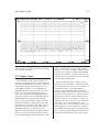
Spectrum Analysis of Wow & Flutter . . . . . . . . . . . . . . . . . . . . . . . . . . . . . . . . . . . . . . . . 17-3
Standards and Test Methods. . . . . . . . . . . . . . . . . . . . . . . . . . . . . . . . . . . . . . . . . . . . . . 17-4
Display Types. . . . . . . . . . . . . . . . . . . . . . . . . . . . . . . . . . . . . . . . . . . . . . . . . . . . . . . . . . 17-5
SWITCHER MODULES . . . . . . . . . . . . . . . . . . . . . . . . . . . . . . . . . . . . . . . . . . . . . . . . . . . 18-1
Introduction. . . . . . . . . . . . . . . . . . . . . . . . . . . . . . . . . . . . . . . . . . . . . . . . . . . . . . . . . . . . 18-1
Functional Description . . . . . . . . . . . . . . . . . . . . . . . . . . . . . . . . . . . . . . . . . . . . . . . . . . . 18-1
Input Switcher . . . . . . . . . . . . . . . . . . . . . . . . . . . . . . . . . . . . . . . . . . . . . . . . . . . . . . . 18-1
Output Switcher . . . . . . . . . . . . . . . . . . . . . . . . . . . . . . . . . . . . . . . . . . . . . . . . . . . . . 18-1
Patch Point Switcher. . . . . . . . . . . . . . . . . . . . . . . . . . . . . . . . . . . . . . . . . . . . . . . . . . 18-2
Terminal Strip Switcher. . . . . . . . . . . . . . . . . . . . . . . . . . . . . . . . . . . . . . . . . . . . . . . . 18-5
Jumper Selection . . . . . . . . . . . . . . . . . . . . . . . . . . . . . . . . . . . . . . . . . . . . . . . . . . 18-5
Input/Output Connections . . . . . . . . . . . . . . . . . . . . . . . . . . . . . . . . . . . . . . . . . . . 18-5
Installation . . . . . . . . . . . . . . . . . . . . . . . . . . . . . . . . . . . . . . . . . . . . . . . . . . . . . . . . . . . . 18-6
Control of Switchers. . . . . . . . . . . . . . . . . . . . . . . . . . . . . . . . . . . . . . . . . . . . . . . . . . . . . 18-8
Switcher Control Panel . . . . . . . . . . . . . . . . . . . . . . . . . . . . . . . . . . . . . . . . . . . . . . . . 18-8
Driving All But One Channel. . . . . . . . . . . . . . . . . . . . . . . . . . . . . . . . . . . . . . . . . . . . 18-8
Sweep (F9) Definitions Panel . . . . . . . . . . . . . . . . . . . . . . . . . . . . . . . . . . . . . . . . . . . 18-9
Nested Switcher Scans. . . . . . . . . . . . . . . . . . . . . . . . . . . . . . . . . . . . . . . . . . . . . . . 18-10
Typical Switcher Applications . . . . . . . . . . . . . . . . . . . . . . . . . . . . . . . . . . . . . . . . . . . . 18-11
Stereo Control Preamplifier . . . . . . . . . . . . . . . . . . . . . . . . . . . . . . . . . . . . . . . . . . . 18-11
Multi-track Tape Recorder . . . . . . . . . . . . . . . . . . . . . . . . . . . . . . . . . . . . . . . . . . . . 18-12
Audio Chain or Mixing Console Channel . . . . . . . . . . . . . . . . . . . . . . . . . . . . . . . . . 18-16
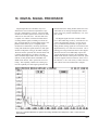
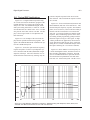
DIGITAL SIGNAL PROCESSOR . . . . . . . . . . . . . . . . . . . . . . . . . . . . . . . . . . . . . . . . . . . . 19-1
Typical DSP Applications. . . . . . . . . . . . . . . . . . . . . . . . . . . . . . . . . . . . . . . . . . . . . . . . . 19-3
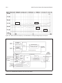
DSP Architecture . . . . . . . . . . . . . . . . . . . . . . . . . . . . . . . . . . . . . . . . . . . . . . . . . . . . . . . 19-5
Downloading DSP Programs . . . . . . . . . . . . . . . . . . . . . . . . . . . . . . . . . . . . . . . . . . . . . . 19-5
DSP Input Operation . . . . . . . . . . . . . . . . . . . . . . . . . . . . . . . . . . . . . . . . . . . . . . . . . . . . 19-6
Rate vs Bandwidth . . . . . . . . . . . . . . . . . . . . . . . . . . . . . . . . . . . . . . . . . . . . . . . . . . . 19-6
5
6
Audio Precision System One User's Manual
Dither . . . . . . . . . . . . . . . . . . . . . . . . . . . . . . . . . . . . . . . . . . . . . . . . . . . . . . . . . . . . . 19-7
AES/EBU Status Bytes . . . . . . . . . . . . . . . . . . . . . . . . . . . . . . . . . . . . . . . . . . . . . . . 19-7
BURST-SQUAREWAVE-NOISE GENERATOR . . . . . . . . . . . . . . . . . . . . . . . . . . . . . . . .
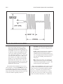
Tone Burst Waveforms . . . . . . . . . . . . . . . . . . . . . . . . . . . . . . . . . . . . . . . . . . . . . . . . . .
Triggered Bursts . . . . . . . . . . . . . . . . . . . . . . . . . . . . . . . . . . . . . . . . . . . . . . . . . . . .
Gated Sinewaves. . . . . . . . . . . . . . . . . . . . . . . . . . . . . . . . . . . . . . . . . . . . . . . . . . . .
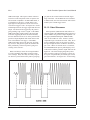
Squarewaves. . . . . . . . . . . . . . . . . . . . . . . . . . . . . . . . . . . . . . . . . . . . . . . . . . . . . . . . . .
Noise Waveforms . . . . . . . . . . . . . . . . . . . . . . . . . . . . . . . . . . . . . . . . . . . . . . . . . . . . . .
Pseudo and Random Noise. . . . . . . . . . . . . . . . . . . . . . . . . . . . . . . . . . . . . . . . . . . .
White Noise . . . . . . . . . . . . . . . . . . . . . . . . . . . . . . . . . . . . . . . . . . . . . . . . . . . . . . . .
Pink Noise . . . . . . . . . . . . . . . . . . . . . . . . . . . . . . . . . . . . . . . . . . . . . . . . . . . . . . . . .
Bandpass Noise. . . . . . . . . . . . . . . . . . . . . . . . . . . . . . . . . . . . . . . . . . . . . . . . . . . . .
Equalized Bandpass Noise . . . . . . . . . . . . . . . . . . . . . . . . . . . . . . . . . . . . . . . . . . . .
USASI Noise . . . . . . . . . . . . . . . . . . . . . . . . . . . . . . . . . . . . . . . . . . . . . . . . . . . . . . .
20-1
20-1
20-3
20-4
20-5
20-5
20-5
20-5
20-6
20-6
20-6
20-6
DCX-127 DC AND DIGITAL I/O MODULE. . . . . . . . . . . . . . . . . . . . . . . . . . . . . . . . . . . .
Voltage and Resistance Measurements . . . . . . . . . . . . . . . . . . . . . . . . . . . . . . . . . . . . .
Dc Voltage Measurements . . . . . . . . . . . . . . . . . . . . . . . . . . . . . . . . . . . . . . . . . . . .
Resistance Measurements . . . . . . . . . . . . . . . . . . . . . . . . . . . . . . . . . . . . . . . . . . . .
Offset and Scaling . . . . . . . . . . . . . . . . . . . . . . . . . . . . . . . . . . . . . . . . . . . . . . . . . .
DC Voltage Outputs . . . . . . . . . . . . . . . . . . . . . . . . . . . . . . . . . . . . . . . . . . . . . . . . . . . .
Digital Input . . . . . . . . . . . . . . . . . . . . . . . . . . . . . . . . . . . . . . . . . . . . . . . . . . . . . . . . . .
Digital Output . . . . . . . . . . . . . . . . . . . . . . . . . . . . . . . . . . . . . . . . . . . . . . . . . . . . . . . . .
Program Control Input. . . . . . . . . . . . . . . . . . . . . . . . . . . . . . . . . . . . . . . . . . . . . . . . . . .
Program Control Outputs . . . . . . . . . . . . . . . . . . . . . . . . . . . . . . . . . . . . . . . . . . . . . . . .
Digital Control Output Ports . . . . . . . . . . . . . . . . . . . . . . . . . . . . . . . . . . . . . . . . . . . . . .
21-1
21-1
21-2
21-2
21-2
21-3
21-3
21-4
21-5
21-6
21-7
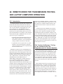
REMOTE MODE FOR TRANSMISSION TESTING AND LAPTOP
COMPUTER OPERATION . . . . . . . . . . . . . . . . . . . . . . . . . . . . . . . . . . . . . . . . . . . . . . 22-1
Introduction . . . . . . . . . . . . . . . . . . . . . . . . . . . . . . . . . . . . . . . . . . . . . . . . . . . . . . . . . . . 22-1
System Architecture, Testing at Two Locations with Two Computers
and “A” Version Systems . . . . . . . . . . . . . . . . . . . . . . . . . . . . . . . . . . . . . . . . . . . . . . . . 22-1
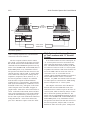
System Architecture, Testing at Two Locations with “S” Version System . . . . . . . . . . 22-2
System Architecture, Laptop/Notebook Computers . . . . . . . . . . . . . . . . . . . . . . . . . . . . 22-3
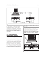
Master and Slave; General Concepts. . . . . . . . . . . . . . . . . . . . . . . . . . . . . . . . . . . . . . . 22-3
Control Computer Operation . . . . . . . . . . . . . . . . . . . . . . . . . . . . . . . . . . . . . . . . . . . . . . 22-4
Remote System Operation . . . . . . . . . . . . . . . . . . . . . . . . . . . . . . . . . . . . . . . . . . . . . . . 22-4
Laptop Computers with “S” Version Systems . . . . . . . . . . . . . . . . . . . . . . . . . . . . . . 22-5
Transmission Testing with “S” Version System. . . . . . . . . . . . . . . . . . . . . . . . . . . . . 22-6
Modem Usage with “S” Version System One . . . . . . . . . . . . . . . . . . . . . . . . . . . 22-6
Transmission Testing with Two Computers . . . . . . . . . . . . . . . . . . . . . . . . . . . . . . . 22-8
“S” Version System One, General Information . . . . . . . . . . . . . . . . . . . . . . . . . . . . . . . . 22-9
“S” Version Switch Settings . . . . . . . . . . . . . . . . . . . . . . . . . . . . . . . . . . . . . . . . . . . 22-10
“S” Version Technical Details . . . . . . . . . . . . . . . . . . . . . . . . . . . . . . . . . . . . . . . . . 22-11
DOS Mode Command. . . . . . . . . . . . . . . . . . . . . . . . . . . . . . . . . . . . . . . . . . . . . . . . . . 22-11
Command Line Options . . . . . . . . . . . . . . . . . . . . . . . . . . . . . . . . . . . . . . . . . . . . . . . . 22-12
Error Messages. . . . . . . . . . . . . . . . . . . . . . . . . . . . . . . . . . . . . . . . . . . . . . . . . . . . . . . 22-13
TABLE OF CONTENTS
Creating, Running, Viewing, and Editing Remote Test Files . . . . . . . . . . . . . . . . . . . . 22-13
EQUALIZATION . . . . . . . . . . . . . . . . . . . . . . . . . . . . . . . . . . . . . . . . . . . . . . . . . . . . . . . . . 23-1
Equalization Concepts and Applications . . . . . . . . . . . . . . . . . . . . . . . . . . . . . . . . . . . . . 23-1
Using Furnished EQ Files . . . . . . . . . . . . . . . . . . . . . . . . . . . . . . . . . . . . . . . . . . . . . . . . 23-1
Creating Equalization Files from Formulas . . . . . . . . . . . . . . . . . . . . . . . . . . . . . . . . . . . 23-3
Entering and Editing Equalization Files . . . . . . . . . . . . . . . . . . . . . . . . . . . . . . . . . . . . . . 23-4
Creating EQ Files from Measured Data . . . . . . . . . . . . . . . . . . . . . . . . . . . . . . . . . . . . . 23-4
ACCEPTANCE TEST LIMITS . . . . . . . . . . . . . . . . . . . . . . . . . . . . . . . . . . . . . . . . . . . . . . 24-1
Creating A Limit File . . . . . . . . . . . . . . . . . . . . . . . . . . . . . . . . . . . . . . . . . . . . . . . . . . . . 24-1
Creating the Test for Use With Limits Files. . . . . . . . . . . . . . . . . . . . . . . . . . . . . . . . . . . 24-2
Creating Limits Files By Actual Tests . . . . . . . . . . . . . . . . . . . . . . . . . . . . . . . . . . . . . . . 24-3
Running Tests With Limits . . . . . . . . . . . . . . . . . . . . . . . . . . . . . . . . . . . . . . . . . . . . . . . . 24-3
Master Error Files . . . . . . . . . . . . . . . . . . . . . . . . . . . . . . . . . . . . . . . . . . . . . . . . . . . . . . 24-4
PROCEDURES . . . . . . . . . . . . . . . . . . . . . . . . . . . . . . . . . . . . . . . . . . . . . . . . . . . . . . . . . . 25-1
Loading and Running Procedures . . . . . . . . . . . . . . . . . . . . . . . . . . . . . . . . . . . . . . . . . . 25-1
Generating Procedures . . . . . . . . . . . . . . . . . . . . . . . . . . . . . . . . . . . . . . . . . . . . . . . . . . 25-2
Generating Procedures by Learning Keystrokes . . . . . . . . . . . . . . . . . . . . . . . . . . . . 25-2
Learn Mode Procedure Example. . . . . . . . . . . . . . . . . . . . . . . . . . . . . . . . . . . . . . 25-2
Creating or Modifying Procedures in Edit Mode . . . . . . . . . . . . . . . . . . . . . . . . . . . . 25-3
Adding to Existing Procedures. . . . . . . . . . . . . . . . . . . . . . . . . . . . . . . . . . . . . . . . . . . . . 25-4
Program Flow Control . . . . . . . . . . . . . . . . . . . . . . . . . . . . . . . . . . . . . . . . . . . . . . . . . . . 25-5
Jumping to Another Location: UTIL GOTO. . . . . . . . . . . . . . . . . . . . . . . . . . . . . . . . 25-6
Conditional Branching: IF . . . . . . . . . . . . . . . . . . . . . . . . . . . . . . . . . . . . . . . . . . . . . 25-6
Conditional Branching Upon Operator Input . . . . . . . . . . . . . . . . . . . . . . . . . . . . . . . 25-6
Sub-Procedures . . . . . . . . . . . . . . . . . . . . . . . . . . . . . . . . . . . . . . . . . . . . . . . . . . . . . 25-6
Sub-Procedure Example: Printing Only Upon Error . . . . . . . . . . . . . . . . . . . . . . 25-7
Example: Looping On Error. . . . . . . . . . . . . . . . . . . . . . . . . . . . . . . . . . . . . . . . . . . . 25-8
Sub-Procedure Example: Test Menu . . . . . . . . . . . . . . . . . . . . . . . . . . . . . . . . . . . . 25-8
Changes in Panel Setup During a Procedure . . . . . . . . . . . . . . . . . . . . . . . . . . . . . . . . . 25-9
Two-Character Codes to Jump to Panel Fields . . . . . . . . . . . . . . . . . . . . . . . . . . . . 25-10
Partial Loads (Overlays) to Protect Panel Fields . . . . . . . . . . . . . . . . . . . . . . . . . . . . . 25-10
Creating Overlays . . . . . . . . . . . . . . . . . . . . . . . . . . . . . . . . . . . . . . . . . . . . . . . . . . . 25-11
Appearance of Blanked Fields . . . . . . . . . . . . . . . . . . . . . . . . . . . . . . . . . . . . . . . . . 25-11
Interrupting or Pausing Procedures . . . . . . . . . . . . . . . . . . . . . . . . . . . . . . . . . . . . . . . . 25-12
Prompts, Pauses, and Delays . . . . . . . . . . . . . . . . . . . . . . . . . . . . . . . . . . . . . . . . . . . . 25-12
De-Bugging Procedures by Single Stepping . . . . . . . . . . . . . . . . . . . . . . . . . . . . . . . . 25-13
Creating a Form to be Filled In . . . . . . . . . . . . . . . . . . . . . . . . . . . . . . . . . . . . . . . . . . . 25-13
Control of External Devices . . . . . . . . . . . . . . . . . . . . . . . . . . . . . . . . . . . . . . . . . . . . . . 25-14
Inserting DOS Commands in a Procedure . . . . . . . . . . . . . . . . . . . . . . . . . . . . . . . . . . 25-15
Limits, Error Files, and Data Management . . . . . . . . . . . . . . . . . . . . . . . . . . . . . . . . . . 25-15
Storing Data in Subdirectories . . . . . . . . . . . . . . . . . . . . . . . . . . . . . . . . . . . . . . . . . 25-16
System Startup With Procedure Running . . . . . . . . . . . . . . . . . . . . . . . . . . . . . . . . . . . 25-17
Continuously-Running Procedures . . . . . . . . . . . . . . . . . . . . . . . . . . . . . . . . . . . . . . . . 25-18
Signal-to-Noise Ratio Tests in Procedures . . . . . . . . . . . . . . . . . . . . . . . . . . . . . . . . . . 25-18
7
8
Audio Precision System One User's Manual
REGULATION . . . . . . . . . . . . . . . . . . . . . . . . . . . . . . . . . . . . . . . . . . . . . . . . . . . . . . . . . .
Introduction . . . . . . . . . . . . . . . . . . . . . . . . . . . . . . . . . . . . . . . . . . . . . . . . . . . . . . . . . . .
Regulation Concept. . . . . . . . . . . . . . . . . . . . . . . . . . . . . . . . . . . . . . . . . . . . . . . . . . . . .
Regulation Panel. . . . . . . . . . . . . . . . . . . . . . . . . . . . . . . . . . . . . . . . . . . . . . . . . . . . . . .
Regulation Algorithms . . . . . . . . . . . . . . . . . . . . . . . . . . . . . . . . . . . . . . . . . . . . . . . . . . .
Success In Regulation . . . . . . . . . . . . . . . . . . . . . . . . . . . . . . . . . . . . . . . . . . . . . . . . . .
Setting Up A Regulation Test . . . . . . . . . . . . . . . . . . . . . . . . . . . . . . . . . . . . . . . . . . . . .
Data Display . . . . . . . . . . . . . . . . . . . . . . . . . . . . . . . . . . . . . . . . . . . . . . . . . . . . . . . . . .
26-1
26-1
26-1
26-1
26-2
26-4
26-5
26-6
TESTING SPEED . . . . . . . . . . . . . . . . . . . . . . . . . . . . . . . . . . . . . . . . . . . . . . . . . . . . . . .
Time Per Step . . . . . . . . . . . . . . . . . . . . . . . . . . . . . . . . . . . . . . . . . . . . . . . . . . . . . . . . .
Sweep Time . . . . . . . . . . . . . . . . . . . . . . . . . . . . . . . . . . . . . . . . . . . . . . . . . . . . . . . . . .
Limits and Speed . . . . . . . . . . . . . . . . . . . . . . . . . . . . . . . . . . . . . . . . . . . . . . . . . . . . . .
Equalization and Speed . . . . . . . . . . . . . . . . . . . . . . . . . . . . . . . . . . . . . . . . . . . . . . . . .
Graphics Save Mode and Speed . . . . . . . . . . . . . . . . . . . . . . . . . . . . . . . . . . . . . . . . . .
Disk Types and Testing Speed. . . . . . . . . . . . . . . . . . . . . . . . . . . . . . . . . . . . . . . . . . . .
Virtual Disks . . . . . . . . . . . . . . . . . . . . . . . . . . . . . . . . . . . . . . . . . . . . . . . . . . . . . . . .
Computer Types and Speed. . . . . . . . . . . . . . . . . . . . . . . . . . . . . . . . . . . . . . . . . . . . . .
FASTEST.DSP and Speed . . . . . . . . . . . . . . . . . . . . . . . . . . . . . . . . . . . . . . . . . . . . . . .
Software and Speed . . . . . . . . . . . . . . . . . . . . . . . . . . . . . . . . . . . . . . . . . . . . . . . . . . . .
27-1
27-1
27-2
27-2
27-2
27-3
27-3
27-3
27-4
27-4
27-4
CREATING YOUR CUSTOM SOFTWARE START-UP PROCESS . . . . . . . . . . . . . . . .
Making A Bootable Diskette . . . . . . . . . . . . . . . . . . . . . . . . . . . . . . . . . . . . . . . . . . . . . .
Creating an AUTOEXEC.BAT File . . . . . . . . . . . . . . . . . . . . . . . . . . . . . . . . . . . . . . . . .
Testing The Startup Process . . . . . . . . . . . . . . . . . . . . . . . . . . . . . . . . . . . . . . . . . . . . .
STD.TST File to Set Initial Conditions . . . . . . . . . . . . . . . . . . . . . . . . . . . . . . . . . . . . . .
Command Line Options . . . . . . . . . . . . . . . . . . . . . . . . . . . . . . . . . . . . . . . . . . . . . . . . .
Starting With a Specific Test or Procedure . . . . . . . . . . . . . . . . . . . . . . . . . . . . . . . .
Starting Up With the Last Test . . . . . . . . . . . . . . . . . . . . . . . . . . . . . . . . . . . . . . . . .
Graphics System Compatibility . . . . . . . . . . . . . . . . . . . . . . . . . . . . . . . . . . . . . . . . .
Interface Card Locations . . . . . . . . . . . . . . . . . . . . . . . . . . . . . . . . . . . . . . . . . . . . . .
Controlling Memory Usage . . . . . . . . . . . . . . . . . . . . . . . . . . . . . . . . . . . . . . . . . . . .
System One Memory Requirements . . . . . . . . . . . . . . . . . . . . . . . . . . . . . . . . . .
Memory Reserved for Programs to Run Under XDOS or DOS Exit . . . . . . . . . .
Screen Display Memory . . . . . . . . . . . . . . . . . . . . . . . . . . . . . . . . . . . . . . . . . . . .
Internal Buffers of S1.EXE . . . . . . . . . . . . . . . . . . . . . . . . . . . . . . . . . . . . . . . . . .
Data Point Buffer . . . . . . . . . . . . . . . . . . . . . . . . . . . . . . . . . . . . . . . . . . . . . . . . .
Limit/Sweep/EQ File Buffer . . . . . . . . . . . . . . . . . . . . . . . . . . . . . . . . . . . . . . . . .
Edit Data Buffer . . . . . . . . . . . . . . . . . . . . . . . . . . . . . . . . . . . . . . . . . . . . . . . . . .
Edit Procedure Buffer . . . . . . . . . . . . . . . . . . . . . . . . . . . . . . . . . . . . . . . . . . . . . .
Edit Comment Buffer . . . . . . . . . . . . . . . . . . . . . . . . . . . . . . . . . . . . . . . . . . . . . .
Edit Macro Buffer . . . . . . . . . . . . . . . . . . . . . . . . . . . . . . . . . . . . . . . . . . . . . . . . .
Buffer Size Control . . . . . . . . . . . . . . . . . . . . . . . . . . . . . . . . . . . . . . . . . . . . . . . .
Buffer Swap to Disk . . . . . . . . . . . . . . . . . . . . . . . . . . . . . . . . . . . . . . . . . . . . . . .
Screen Appearance of Punched-Out Fields . . . . . . . . . . . . . . . . . . . . . . . . . . . . . . .
Printer Mode and Printed Graph Size Selection . . . . . . . . . . . . . . . . . . . . . . . . . . .
28-1
28-1
28-1
28-2
28-3
28-3
28-4
28-4
28-4
28-5
28-5
28-5
28-6
28-6
28-7
28-7
28-7
28-7
28-7
28-7
28-8
28-8
28-9
28-9
28-9
TABLE OF CONTENTS
Formatting of Graph Printout . . . . . . . . . . . . . . . . . . . . . . . . . . . . . . . . . . . . . . . . . . 28-10
Plotter and Laser Printer Compatibility . . . . . . . . . . . . . . . . . . . . . . . . . . . . . . . . . . . 28-10
Command Line Query. . . . . . . . . . . . . . . . . . . . . . . . . . . . . . . . . . . . . . . . . . . . . . . . 28-10
Batch Files for Loading S1.EXE . . . . . . . . . . . . . . . . . . . . . . . . . . . . . . . . . . . . . . . . 28-10
Using the Environment to Control Start-Up . . . . . . . . . . . . . . . . . . . . . . . . . . . . . . . 28-11
MOUSE OPERATION. . . . . . . . . . . . . . . . . . . . . . . . . . . . . . . . . . . . . . . . . . . . . . . . . . . . . 29-1
Introduction. . . . . . . . . . . . . . . . . . . . . . . . . . . . . . . . . . . . . . . . . . . . . . . . . . . . . . . . . . . . 29-1
Mouse Compatibility, PCI-1 Card . . . . . . . . . . . . . . . . . . . . . . . . . . . . . . . . . . . . . . . . . . 29-1
Mouse Compatibility, PCI-2 Card . . . . . . . . . . . . . . . . . . . . . . . . . . . . . . . . . . . . . . . . . . 29-1
PCI-2 Installation with Bus Mouse . . . . . . . . . . . . . . . . . . . . . . . . . . . . . . . . . . . . . . . 29-1
PCI-2 Installation with Serial Mouse. . . . . . . . . . . . . . . . . . . . . . . . . . . . . . . . . . . . . . 29-1
PCI-3 Installation with Mouse . . . . . . . . . . . . . . . . . . . . . . . . . . . . . . . . . . . . . . . . . . . . . 29-2
Mouse Software Installation. . . . . . . . . . . . . . . . . . . . . . . . . . . . . . . . . . . . . . . . . . . . . . . 29-2
Mouse Usage . . . . . . . . . . . . . . . . . . . . . . . . . . . . . . . . . . . . . . . . . . . . . . . . . . . . . . . . . . 29-2
COMPUTER MONITOR NOISE FIELDS . . . . . . . . . . . . . . . . . . . . . . . . . . . . . . . . . . . . . . 30-1
AUDIO TESTING . . . . . . . . . . . . . . . . . . . . . . . . . . . . . . . . . . . . . . . . . . . . . . . . . . . . . . . . 31-1
Introduction. . . . . . . . . . . . . . . . . . . . . . . . . . . . . . . . . . . . . . . . . . . . . . . . . . . . . . . . . . . . 31-1
Amplitude or Level Measurements . . . . . . . . . . . . . . . . . . . . . . . . . . . . . . . . . . . . . . . . . 31-1
Frequency Response . . . . . . . . . . . . . . . . . . . . . . . . . . . . . . . . . . . . . . . . . . . . . . . . . 31-1
Frequency Response at Constant Output Amplitude. . . . . . . . . . . . . . . . . . . . . . . . . 31-2
Testing Pre-Emphasized Transmitters . . . . . . . . . . . . . . . . . . . . . . . . . . . . . . . . . 31-3
Frequency Response of Compact Disc Players. . . . . . . . . . . . . . . . . . . . . . . . . . . . . 31-3
Frequency Response of Tape Recorders and Players . . . . . . . . . . . . . . . . . . . . . . . 31-4
Three Head Machines . . . . . . . . . . . . . . . . . . . . . . . . . . . . . . . . . . . . . . . . . . . . . . 31-4
Determining Tape Recorder Delay . . . . . . . . . . . . . . . . . . . . . . . . . . . . . . . . . . . . 31-4
Two Head Machines . . . . . . . . . . . . . . . . . . . . . . . . . . . . . . . . . . . . . . . . . . . . . . . 31-5
Recording a Test Tape . . . . . . . . . . . . . . . . . . . . . . . . . . . . . . . . . . . . . . . . . . . . . 31-5
Playback Frequency Response. . . . . . . . . . . . . . . . . . . . . . . . . . . . . . . . . . . . . . . 31-5
Gain and Loss. . . . . . . . . . . . . . . . . . . . . . . . . . . . . . . . . . . . . . . . . . . . . . . . . . . . . . . 31-6
Signal to Noise Ratio . . . . . . . . . . . . . . . . . . . . . . . . . . . . . . . . . . . . . . . . . . . . . . . . . 31-6
Absolute Noise Tests . . . . . . . . . . . . . . . . . . . . . . . . . . . . . . . . . . . . . . . . . . . . . . . . . 31-7
Non-Linearity Tests . . . . . . . . . . . . . . . . . . . . . . . . . . . . . . . . . . . . . . . . . . . . . . . . . . . . . 31-7
Harmonic Distortion Concepts . . . . . . . . . . . . . . . . . . . . . . . . . . . . . . . . . . . . . . . . . . 31-7
SMPTE/DIN Intermodulation Concepts . . . . . . . . . . . . . . . . . . . . . . . . . . . . . . . . . . . 31-7
CCIF Intermodulation Concepts . . . . . . . . . . . . . . . . . . . . . . . . . . . . . . . . . . . . . . . . . 31-8
DIM/TIM Intermodulation Concepts . . . . . . . . . . . . . . . . . . . . . . . . . . . . . . . . . . . . . . 31-8
Distortion Versus Amplitude . . . . . . . . . . . . . . . . . . . . . . . . . . . . . . . . . . . . . . . . . . . . 31-8
Distortion Versus Frequency . . . . . . . . . . . . . . . . . . . . . . . . . . . . . . . . . . . . . . . . . . . 31-8
Distortion at Constant Power Tests . . . . . . . . . . . . . . . . . . . . . . . . . . . . . . . . . . . . . . 31-9
Tape Recorder Non-Linearity . . . . . . . . . . . . . . . . . . . . . . . . . . . . . . . . . . . . . . . . . . . 31-9
Distortion Versus Frequency of Tape Recorders . . . . . . . . . . . . . . . . . . . . . . . . . 31-9
Compact Disc Player Non-Linearity . . . . . . . . . . . . . . . . . . . . . . . . . . . . . . . . . . . . . 31-10
CD Player THD+N Versus Frequency . . . . . . . . . . . . . . . . . . . . . . . . . . . . . . . . 31-10
Quantization Distortion . . . . . . . . . . . . . . . . . . . . . . . . . . . . . . . . . . . . . . . . . . . . 31-10
Phase Measurements . . . . . . . . . . . . . . . . . . . . . . . . . . . . . . . . . . . . . . . . . . . . . . . . . . 31-12
9
10
Audio Precision System One User's Manual
Input-Output Phase Measurements. . . . . . . . . . . . . . . . . . . . . . . . . . . . . . . . . . . . . 31-12
Interchannel Phase Measurements . . . . . . . . . . . . . . . . . . . . . . . . . . . . . . . . . . . . . 31-12
Tape Recorder Azimuth Adjustments . . . . . . . . . . . . . . . . . . . . . . . . . . . . . . . . . . . 31-13
ANALYZER AND GENERATOR HARDWARE . . . . . . . . . . . . . . . . . . . . . . . . . . . . . . . .
Analyzer Block Diagram . . . . . . . . . . . . . . . . . . . . . . . . . . . . . . . . . . . . . . . . . . . . . . . . .
Generator Block Diagram . . . . . . . . . . . . . . . . . . . . . . . . . . . . . . . . . . . . . . . . . . . . . . . .
Intermodulation Test Signal Generation Hardware . . . . . . . . . . . . . . . . . . . . . . . . . .
BUR Option Hardware . . . . . . . . . . . . . . . . . . . . . . . . . . . . . . . . . . . . . . . . . . . . . . . .
Auxiliary Generator Connectors. . . . . . . . . . . . . . . . . . . . . . . . . . . . . . . . . . . . . . . . .
32-1
32-1
32-4
32-4
32-4
32-5
S1.EXE ERROR REPORTING DESCRIPTIONS . . . . . . . . . . . . . . . . . . . . . . . . . . . . . . . 33-1
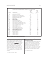
FURNISHED DISK FILE DESCRIPTIONS . . . . . . . . . . . . . . . . . . . . . . . . . . . . . . . . . . . .
S1.EXE version: 2.10 Diskette . . . . . . . . . . . . . . . . . . . . . . . . . . . . . . . . . . . . . . . . . . . .
Test and Procedures Diskette . . . . . . . . . . . . . . . . . . . . . . . . . . . . . . . . . . . . . . . . . . . .
Utilities and Equalization Diskette. . . . . . . . . . . . . . . . . . . . . . . . . . . . . . . . . . . . . . . . . .
34-1
34-1
34-1
34-6
INDEX . . . . . . . . . . . . . . . . . . . . . . . . . . . . . . . . . . . . . . . . . . . . . . . . . . . . . . . . . . . . . . . . 35-1
1. UNPACK AND INVENTORY
Your new System One comes packed in a carton
which also contains the interface card, cable, software, and documentation. Check to be sure that you
have received:
a. System One enclosure with all modules and
options which you ordered installed (check the packing list for specific options)
b. PCI plug-in interface card for installation in
computer (unless you ordered the “S” or “G” versions of System One)
c. cable with 25-pin connectors to connect System One to computer interface card (unless you ordered the “S” or “G” versions of System One)
d. ac power line cord
e. two training videotapes in the appropriate
video standard for your area. The basic operator’s
training videotape is APV-1 and the advanced training videotape is APV-2
f. this User’s Manual, with diskettes containing
System One software
If your order also included the DCX-127 module
or SWR-122 family of switchers, each of these modules will be shipped in a separate carton with a 0.5
meter digital interface cable and an ac power line
cord.
It is recommended that you save the carton(s) in
case it is ever necessary to ship System One.
1-1
1-2
Audio Precision System One Operator's Manual
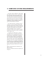
2. COMPUTER SYSTEM REQUIREMENTS
System One requires an IBM PC or fully compatible computer in order to operate. System One has
been successfully operated with computers using
8088, 8086, 80286, 80386, and 80486 microprocessors. With well over 2,000 units of System One in
operation, there have been no reports of incompatibility between System One and any PC-compatible
computer with either the original PC bus or the Microchannel bus. The PCI-3 interface card is required for Microchannel bus computers.
The computer must have a minimum of 640 kb
of memory. It must be operating with DOS (disk
operating system) Version 2.2 or later. It must contain a color graphics card (CGA), enhanced graphics
card (EGA), video graphics array card (VGA),
Toshiba 3100 display system, or a Hercules (TM)
monochrome graphics card or equivalent, driving a
monochrome or color monitor which is compatible
with the graphics card.
A minimum of one diskette drive is required.
Two diskette drives or one diskette drive and one
hard disk drive are recommended for the most convenient operation. The hard disk, or configuring
part of the computer memory as virtual disk (ram
disk) is particularly recommended for applications
where procedures will be used (see PROCEDURES
chapter) or where data or error file information from
tests will be saved. It is strongly recommended that
a math co-processor be installed (8087 for 8088 and
8086-based computers; 80287 for 80286-based computers). System One will operate without it, but operating speed is greatly enhanced by the co-processor.
IBM PC and Microchannel are trademarks of the
IBM Corporation.
Hercules is a trademark of Hercules Computer Technology, Inc.
2-1
2-2
Audio Precision System One Operator's Manual
3. INSTALLING THE INTERFACE CARD
An interface card must be installed in the computer for operation of of the original and “A” versions of System One. Neither the “S” (serial, or RS232) version nor the “G” (GPIB) version requires an
interface card. See the special operator’s manual
supplement furnished with “S” version systems for
information on preparation of the computer.
Audio Precision has manufactured three versions
of interface card. All contain a 25-pin female connector for the digital interface cable to System One.
The PCI-1 card (no longer in production) contains a
second connector , a 9-pin female subminiature D
type connector for connection to an original version
Microsoft bus (parallel) mouse. The PCI-1 card is
compatible only with this original version bus
mouse; it is not compatible with the later version
bus mouse which has a round DIN style connector.
The PCI-2 interface card contains a 9-pin male
subminiature D type connector for use as a serial
port. The PCI-2 card is compatible with either a se-
rial mouse, or a parallel mouse with its own interface card. The bottom edge of either the PCI-1 or
PCI-2 card consists of gold-plated contacts to plug
into the computer “mother board”.
The PCI-3 card is designed for the IBM Microchannel bus in the more powerful models of the
PS/2 series; it contains neither mouse nor RS-232
port.
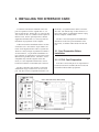
3.1. Card Preparation Before
Installation
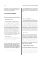
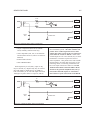
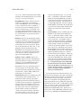
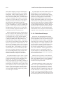
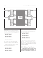
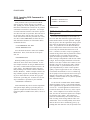
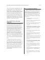
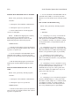
3.1.1. PCI-2 Card Preparation
If the PCI-2 card serial port is not required and a
bus mouse will not be installed, the PCI-2 card can
be installed without further preparation.
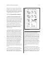
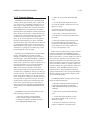
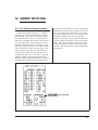
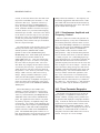
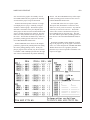
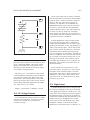
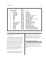
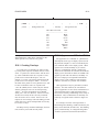
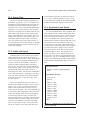
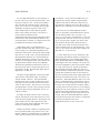
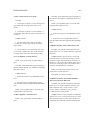
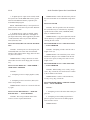
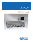
Figure 3-1 Jumper Locations, PCI-2 Card
3-1
3-2
Audio Precision System One Operator's Manual
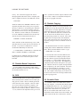
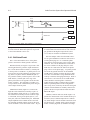
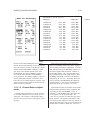
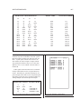
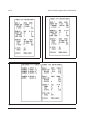
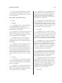
JUMPER
P321
P322
P323
P324
ADDRESS
238H
298H
2B8H
2D8H
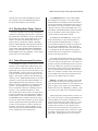
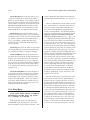
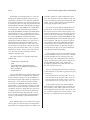
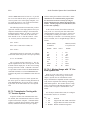
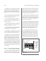
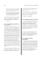
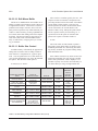
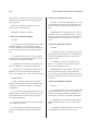
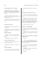
Figure 3-3 PCI-2 I/O Address Jumper Location
If the PCI-2 card is to be installed in the computer along with a bus (parallel) mouse interface
card, address conflict may occur. If so, a jumper
must be moved on the PCI-2 card to place it at a different I/O address in the computer to avoid conflict
with the mouse interface card. Once the jumper is
moved, however, only version 1.60 or later software
may be used with this card.
The PCI-2 card is shipped with the address set to
238 hexadecimal. All PCI-1 cards were fixed at this
same address, and all software versions through 1.50
use this address. Figure 3-3 and Figure 3-1 show
the relationship between jumper position on the PCI2 and the computer I/O address at which System
One will be located. Software versions 1.60 and
later will automatically determine which address the
PCI-2 card is set to and will then communicate with
it properly. See page 28-5 for information on forcing the software to work only with a specific address via the /I option at startup.
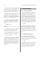
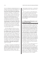
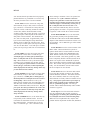
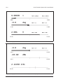
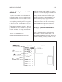
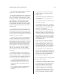
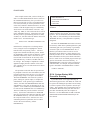
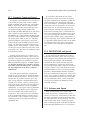
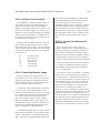
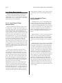
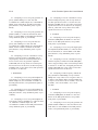
The PCI-2 card contains a serial port which is not
enabled when the card is shipped. This port may be
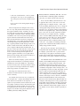
enabled and used for a serial mouse or any other serial port application with System One or other software applications. Note, however, that the IBM-PC
and compatible architecture limits the number of serial ports to a maximum of two. If the serial port is
to be enabled, jumpers must be moved at the P121
location and the P421 location to configure the port
as COM1: or COM2:. Figure 3-2 shows the pins
which must be jumpered together at P121 and P421.
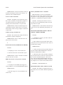
MODE
COM2:
COM1:
OFF
P121
pins 4-5
pins 1-2
pins 3-4
P421
pins 1-2
pins 2-3
no jumper
Figure 3-2 PCI-2 Card Serial Port Configuration
Figure 3-1 shows the location of these pins. Note
also that the DOS MODE command must then be
executed after booting the computer to define communications via this port.
The remaining jumpers which may be noted on
the PCI-2 card are related to possible future DMA
operation of the interface. They should not be used
at this time.
3.1.2. PCI-1 Card Preparation
If an original PCI-1 interface card is being installed or re-installed and you do not have a Microsoft Mouse, be sure the Mouse circuitry is disabled by removing the jumper from positions 2-5.
Store the jumper by plugging it onto the top horizontal row of pins (D1 or D3) at the bottom of the PCI1 interface card, near the gold-plated connector pins.
These two pins are already connected together on
the foil side of the card.
If the PCI-1 is used with the original version of
the bus mouse (9-pin subminiature D connector), the
jumper should normally be on position 2 for the
IBM-PC, XT, and their “clones”, and on position 5
for the IBM-AT and AT “clones”. The PCI-1 interface card duplicates the Microsoft Mouse’s use of interrupts including the jumper-selectable interrupt
number. If the original mouse is used with the PCI1 card, the interrupt number may be set from 2 to 5.
These numbers are etched on the board underneath
the four possible jumper pin locations, just below
the large integrated circuit, where 2 is the position
closest to the cable connectors. In each case, the
jumper must connect a center-row pin to the bottomrow pin immediately below it. The XT and most after-market hard disks use interrupt 5, thus making interrupt 2 the correct position for the mouse. The
AT uses interrupt 2 internally, making 5 the correct
position; however, interrupt 5 may also be associated with a parallel port 2 if present. Interrupt
number 3 is normally associated with serial port 2;
interrupt number 4 is normally associated with serial
port 1.
INSTALLING THE INTERFACE CARD
If the PCI-1 interface card has the jumper installed at the same interrupt location as another device on the computer bus, the result would be malfunction of some portion of the computer system. If
you detect an operational problem which was not
previously present when you first re-start your computer after installing the interface card, move the
jumper.
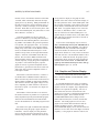
3.2. PCI-2 and PCI-1 Interface Card
Installation
Every different model of computer is likely to
have variations in the process necessary to gain access to its mother board sockets for installation of
the interface card. This manual contains installation
instructions for the IBM PC. Installation in many
desktop units is similar to the IBM PC. In all cases,
disconnect the power cable and all peripheral equipment cables from the computer before starting.
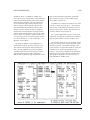
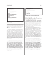
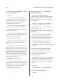
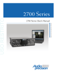
Figure 3-4 IBM PC Cover Removal
3-3
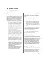
3.2.1. Installation, IBM PC
Remove the cover mounting screws from the rear
of the computer housing (see Figure 3-4), and remove the cover by sliding it off to the front. Locate
the expansion card plug-in area at the rear of the
computer, near the left end. Select a slot into which
you plan to install the System One interface card.
In a computer with a mixture of short and full-size
slots, you may wish to install the System One card
in a short slot. This allows later installation of other
accessories which require long slots. The PCI cards
are not compatible, however, with slot 8 (the last
short slot in PC/XTs) and with the short slot in the
Compaq Deskpro.
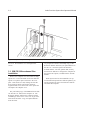
Remove the screw which holds in place the blank
option adapter cover plate (Figure 3-5) immediately
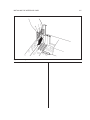
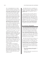
behind the selected slot, and retain the screw. Insert
the interface card into the slot (Figure 3-6) by aligning its gold-plated contact with the computer motherboard socket and pressing the card firmly down into
the socket. Line up the slot in the top edge of the
3-4
Audio Precision System One Operator's Manual
Figure 3-5 Option Adapter Mounting Area
bracket with the screw hole and replace and tighten
the screw. Re-install the cover and tighten the
screws.
3.3. IBM PS/2 Microchannel Bus
Installation
Remove the computer cover and select an empty
option slot. Loosen the thumb screws that hold the
option cover plate in place and remove the cover
plate. Insert the PCI-3 card, making sure that the
PCI-3 board is firmly seated in the connector.
Tighten thumb screws at the back of the option slot
and replace the computer cover.
Put your backup copy of the IBM Reference diskette into drive A: and turn the computer on. The
Reference diskette will boot the computer and put
an IBM logo on the screen. Press <E> to get to the
main menu and select “Copy An Option Diskette”
from the menu.
Follow the prompts as they are given. When you
are prompted to “Remove the backup copy of the
Reference diskette and insert your option diskette in
the drive A” insert the System One Software
S1.EXE diskette. The file, @6064.ADF, used by
the Reference diskette to configure the computer for
the System One option, is included on the S1.EXE
diskette.
When System One has been installed as an option and the backup Reference diskette updated, you
will be prompted to remove the Reference diskette
and restart the computer.
INSTALLING THE INTERFACE CARD
Figure 3-6 Mounting The Interface Card
3-5
3-6
Audio Precision System One Operator's Manual
4. POWER AND CABLE CONNECTIONS
System One and the computer must both be connected to an appropriate ac mains supply. System
One and the DCX-127 can operate from 100 volts,
120 volts, 220 volts, or 240 volts ac (+5/-10% in
each case), 48-63 Hz ac. The ac mains connector/fuse holder assembly on the chassis rear contains
an adapter card which selects the transformer taps
for the line voltage. It must be inserted in the correct one of four possible positions, depending on the
ac line voltage with which System One will be used.
At the same time, a fuse of the proper current rating
must be installed. For 100 or 120 volts, System
One requires a two ampere fuse must be used; for
220 or 240 volts, System One needs a one ampere
fuse. The DCX-127 uses an 0.2 ampere slow blow
fuse on all line voltages. After installing the correct
fuse, hold the adapter card so that the desired line
voltage is upright and readable as you start to insert
the card into the connector assembly while facing
the System One enclosure from the rear. Slide the
card fully into place. Slide the transparent protective cover over the card/fuse area. Connect an appropriate ac mains cable between the connector and
the source of power.
System One is designed with a protective ground
(earth) connection by way of the grounding connector in the power cord. This is essential for safe operation. Do not attempt to defeat its purpose. For
optimum performance, it is recommended that both
System One and the computer be connected to the
same ac mains circuit to minimize ground loop
noise.
The SWR-122 module contains a rear-panel 2-position ac mains voltage range switch. It must be set
to the correct range (100-120 V or 220-240 V) for
the mains power. Connect the appropriate ac mains
cables from the SWR modules to the source of
power.
Connect the computer (assuming that it has also
been set for the correct voltage) to the ac power
source.
Connect the male end of the cable furnished with
System One to the interface card installed in the
computer. If no DCX-127 or SWR-122 modules
will be part of the system, connect the female end of
the digital interface cable to the connector on the
rear of the System One enclosure. If DCX or SWR
modules are present, the long cable from the computer should connect to one of them. Short digital
interface cables may then be used to connect additional modules in daisy-chain fashion, with System
One the last unit in the chain. This is necessary
with earlier models of the “A” version of System
One and all “G” or “S” versions when operating in
“A” version mode, since they have only one digital
interface connector. The DCX and SWR modules
and recent “A” version System Ones have both male
and female connectors to permit daisy chaining.
4.1. Generator-Only and
Analyzer-Only Models
System One can be provided as a generator-only
package (SYS-20) and an analyzer-only package
(SYS-02). These units are commonly used in testing broadcast transmission links. When the two
units are used at the same location, two audio cable
connections are required between them so that the
generator monitor (GEN-MON) function will work.
The generator monitor function permits the analyzer
to measure the exact, loaded output voltage from the
generator. It is required for self-test procedures
such as SYS22CK.PRO (included on the Tests and
Utilities diskette) to function. Connect a shielded
audio cable with XLR connectors between the Channel A Generator Monitor connectors of the SYS-20
and SYS-02 packages. Connect another shielded cable between the Channel B Generator Monitor connectors on the two units.
Turn on System One, the DCX-127, and the
computer. The SWR-122 switchers have no power
switch.
4-1
4-2
Audio Precision System One Operator's Manual
5. LOADING THE SOFTWARE
5.1. Two Forms of Software
System One may be software-controlled from an
IBM-PC or compatible in two fashions:
•
The large majority of System One users find
it most efficient and convenient to control the
system from the panels and menus provided
by the standard software furnished, S1.EXE.
S1.EXE provides instant graphic results, analog bar graph indications for adjustments, supports impromptu, unstructured testing, provides structured tests through procedures, supports acceptance test limits for go/no-go testing, and can be operated without prior experience in a programming language. S1.EXE
supports virtually all types of audio testing.
The balance of this User’s Manual (except for
the COMPUTER MONITOR NOISE FIELDS
chapter and ANALYZER AND GENERATOR HARDWARE chapter) deals exclusively with S1.EXE operation.
System One software is furnished on several
diskettes. The principal operating software
for System One is contained in a file named
S1.EXE. Other diskettes contain a number of
example test (.TST) files, procedure (.PRO)
files, equalization (.EQ) files, and limit (.LIM)
files, performance checks, DSP programs if
the unit purchased has DSP capability, plus a
number of general utility programs for use
during non-audio-testing applications of your
computer. Usage of some of the example
tests and procedures will be discussed in the
next chapter.
•
Certain users find it necessary to write their
own code. Examples of applications which
have required user-written programs include
simultaneous control and audio testing of
large audio routing switchers, extensive interaction with robots or device handlers, or testing plus significant post processing such as
statistical computations. Audio Precision of-
fers for sale two libraries which act as extensions to two common Microsoft programming
languages. The LIB-BASIC library is an extension to the Microsoft BASIC Professional
Development System v7.10. The Microsoft
QuickBASIC Extended Environment is included as part of their Professional Development System v7.10. The LIB-C library is an
extension to the Microsoft C language, v5.1
or later. These libraries of call functions allow control of all aspects of System One including the DSP functions, SWR-122 switchers, and DCX-127 hardware from user-written
programs in the language specified. Wellwritten programs in these languages, using
these function libraries, typically operate substantially faster than when the same set of
tests is performed with the standard S1.EXE
software, partially due to the reduction in computer disk accesses.
If the user-written program approach to testing is
relevant, contact Audio Precision or your Audio Precision distributor for information on how to purchase the LIB-C or LIB-BASIC library and documentation. LIB-C and LIB-BASIC replace the earlier LIB-MIX, APBASIC library, and “C” language
functions. The remainder of this manual will deal
with S1.EXE.
5.2. Hard Disk Operation
Most computers in use today have a hard disk
(fixed disk) in addition to one or more diskette
(floppy disk) drives. This section for software installation assumes that your computer is hard-diskbased, that DOS has been installed and the machine
boots from the hard disk, and that proper operation
of all portions of the system (monitor, keyboard,
etc.) has been verified. If your computer does not
have a hard disk, see the “Diskette-Based Computers” section below for instructions.
5-1
5-2
Audio Precision recommends that a specific set
of sub-directories as described below be created on
the hard disk for operation of System One, and that
specific files from the furnished diskettes be copied
into specific hard disk directories.
Audio Precision System One Operator's Manual
Audio Precision recommends the name AUDIO
for the top-level directory of the group which will
hold all distribution software from Audio Precision.
Thus, the specific command from DOS after changing to the root is:
MD AUDIO <Enter>
5.2.1. Upgrading From Earlier
Versions
If earlier versions of S1.EXE, test, procedures,
etc. have already been installed on your computer
and you wish to preserve them for any reason, it is
recommended that you copy them into some archive
sub-directory or onto diskettes. Then, remove the
sub-directories which held the older tests and follow
the installation instructions below. After completing
the installation of the new software, you may copy
back from the archive sub-directories or diskettes
any older procedures and tests which you wish to
continue using. This process will avoid the risk of a
new file in this release over-writing a valuable older
file of the same name and thus destroying your
unique set-up or data. S1.EXE v2.10 will directly
load and use tests from v2.00 and v1.60. If the test
is loaded and saved from v2.10, it will save as a
v2.10 test. Procedures from earlier versions must
have the header changed to PROCEDUREv2.10.
No other changes should be required for non-DSP
procedures written under v2.00. Procedures from
v1.60 or earlier may also require changes if they involved panel cursor movements or if they used certain menu commands which were changed from
v1.60 to v2.00.
To then change the current directory from the
root directory to this new subdirectory, type:
CD AUDIO <Enter>
If the DOS PROMPT command has been executed with the proper arguments (typically done in
the AUTOEXEC.BAT file), you should see the
prompt
:\AUDIO
You may then copy the entire contents of three of
the distribution diskettes into this C:\AUDIO directory. These are the “S1.EXE” diskette, the “Tests &
Procedures” diskette, and the “Utilities & Equalization” diskette. To copy a diskette, place it in the A:
drive and type
COPY A:*.* <Enter>
All files from the diskette will then be copied
into the current sub-directory, which is C:\AUDIO.
For the second and third diskette, it is not necessary
to type this command again. The <F3> function
key, when in normal DOS command mode, repeats
the last-typed DOS command which is then executed by the <Enter> key.
5.2.2. Making Sub-Directories
To make a new first-level sub-directory on a hard
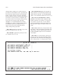
disk (assuming the computer has been booted, type:
CD C:\ <Enter> (CD is the DOS command for
change directory; this command will place you in
the “root”, or top level, directory)
MD dirname <Enter> (MD is the DOS command for make directory; dirname is your desired
new subdirectory name such as AUDIO.
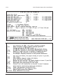
After copying these three diskettes into
C:\AUDIO, made a new sub-directory below this
sub-directory for the contents of the Performance
Checks diskette. With the :\AUDIO prompt visible,
type
MD PERFCHEK <Enter>
This will create a new second-level subdirectory
below the C:\AUDIO directory. To move into this
new directory, type
LOADING THE SOFTWARE
5-3
CD PERFCHEK <Enter>
der AUDIO for the contents of the diskette furnished upon request with the Loudspeaker Testing
(by swept sinewave techniques) Applications Note.
The DOS PROMPT should now read
\AUDIO\PERFCHEK
You can now place the Performance Checks diskette in the A: drive and type
COPY A:*.* <Enter>
If you have other System One-related software, it
is recommended that additional sub-directories under C:\AUDIO be created for each of these. For example, make a sub-directory named COMPDISC under AUDIO for the contents of the Compact Disc
Player testing Applications Note companion diskette. Make a sub-directory named LOUDSPKR un-
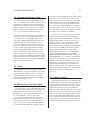
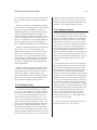
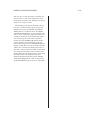
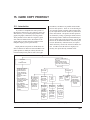
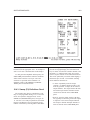
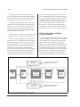
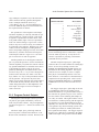
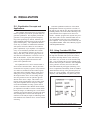
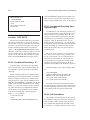
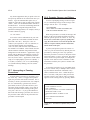
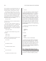
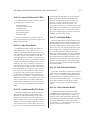
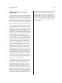
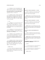
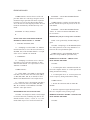
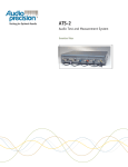
S1.EXE
TEST &
PROCEDURE
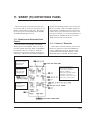
If your System One is a DSP unit, make additional sub-directories under AUDIO named DSP,
FASTEST, MLS, DSPCHEK, and CALIBWAV as
described in the DSP User’s Manual and copy the
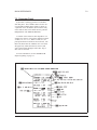
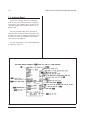
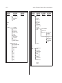
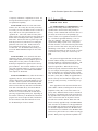
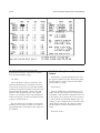
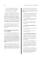
appropriate diskettes into each. See Figure 5-1 for a
schematic representation of the “tree” directory structure with the recommended sub-directory names and
the diskettes which should be copied into each.
As you build up your own collection of customized tests, procedures, and test data files from many
devices under test, you will probably wish to create
additional sub-subdirectories and locate your files
among them according to some organizational plan
appropriate for your work. In general, it is desirable
to never allow more than 88 files of any one type
UTIL & EQ
C:\
(ROOT)
\AUDIO
\PERFCHEK
PERFORM
CHECKS
\DOS
\DSP
DSP FILES
etc.
\UTIL
\COMPDISC
\LOUDSPKR
CD APP
NOTE
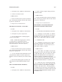
Figure 5-1 Recommended Hard Disk Directory Structure and Location of Distribution Files
SPEAKER
APP NOTE
5-4
(.TST, .PRO, etc.) to exist in one sub-directory since
the S1.EXE “LOAD” command will only display
the first 88 files in the sub-directory.
5.2.3. DOS PATH Command
If the DOS PATH command is not used and the
name of an executable file (.EXE, .COM, or .BAT
file) is typed, DOS looks for that file in the current
directory. If it cannot locate the file, DOS responds
Audio Precision System One Operator's Manual
After adding this sub-directory to the PATH command in AUTOEXEC.BAT, re-boot your computer
for it to take effect. You will then find that you can
type
S1 <Enter>
from any sub-directory on your hard disk and System One software will load.
5.2.4. DOS APPEND Command
Bad command or file name
In order to be able to run S1.EXE and some of
the other utility programs furnished from any sub-directory, it is highly desirable to use the facililty of
the DOS PATH command. The PATH command is
normally placed in your AUTOEXEC.BAT file, so
that it is executed each time your computer is
booted. The PATH command simply contains a list
of all the specific subdirectories you would like to
have DOS look through in an attempt to find the executable file if it is not in the current directory.
With the directory structure and file locations recommended above, only the C:\AUDIO sub-directory
contains any of the furnished executable files. The
form of the PATH command which should be added
to your AUTOEXEC.BAT file is as follows:
PATH C:\AUDIO;
You may find that a PATH command already exists in your AUTOEXEC.BAT file, containing a list
of sub-directories. If so, simply append
C:\AUDIO;
at the end. The semi-colon “;” must be used as a delimiter between consecutive sub-directory names.
For example, if the C:\DOS; and C:\UTIL; sub-directories were already listed in your path command, the
complete list after you have added C:\AUDIO; will
read:
PATH C:\DOS;C:\UTIL;C:\AUDIO
The APPEND command of DOS has a similar effect for non-executable files (often called data files)
to what the PATH command does for executable
files. Whenever an application requires a specific
data file (and the APPEND command is not in use),
the application software looks for the data file in the
current directory. For example, when you run a System One procedure, it expects to find the test files in
the same directory. When a test file is loaded, it expects to find any related limit files, sweep tables,
etc. in the same directory. If a required file cannot
be found in the current directory, the error message
File not found
results. In order that the commonly-used System
One files such as .EQ files, .SWP files, and .DSP
programs (if you have a DSP unit) be usable from
any sub-directory without having to copy them into
every sub-directory which will be used, the APPEND command should be employed. The APPEND command has been part of DOS since DOS
version 3.1. The APPEND command is again typically placed in the AUTOEXEC.BAT file so that it
is executed each time the computer is booted. The
simplest form of the command is:
APPEND C:\dirname1;C:\dirname2;
where dirname1 and dirname2 represents sub-directory names. Execution of this command at the time
the computer is booted will cause DOS to search the
specified directories for any requested data file not
found in the current directory; in effect, those other
specified directories are appended to the current di-
LOADING THE SOFTWARE
rectory. If it is desired to suppress the search
through appended directories when a complete path
name is supplied for the file, the additional “switch”
5-5
puter. System One software requires a DOS version
of 2.2 or later. DOS is not furnished with System
One due to copyright restrictions.
/PATH:OFF
5.5. Diskette Copying
should be added to the APPEND command. This is
frequently desirable when saving tests to a specific
directory or diskette, to avoid getting the “Filename
already exists; Y to overwrite” message if the supplied file name exists in any of the appended directories. With this “switch” added, the recommended
use of the APPEND command for the sub-directory
structure and file location described above is
APPEND C:\AUDIO; /PATH:OFF
which will allow all the furnished .EQ, .TST, .LIM,
and .SWP files to be used from any sub-directory on
the disk. If your unit is a DSP unit, it is recommended that additionally the directories
C:\AUDIO\DSP;C:\AUDIO\MLS;C:\AUDIO\FAST
EST;C:\AUDIO\CALIBWAV; /PATH:OFF
be added onto the APPEND command so that all
DSP programs can be run from anywhere on the
hard disk.
5.3. Diskette-Based Computers
If your computer does not have a hard (fixed)
disk, the following sections describe how to prepare
the furnished software for use.
5.4. DOS
Before S1.EXE can be run, the computer must be
started (booted) with a suitable version of disk operating system, or DOS. DOS is normally purchased
at the same time as the computer. There are different versions of DOS for different computers, and
there may be several versions with progressively
higher revision numbers (DOS 2.2, DOS 2.11, DOS
3.1, etc.) which are all compatible with a given com-
System One software is not copy-protected. It is
good practice to copy the System One diskettes and
use the copies in everyday applications, saving the
distribution disks from Audio Precision in a safe
place. The distribution disks have an adhesive tab
over the notch near the diskette label, to prevent
them from being written on or erased. Your working disk with test and procedure files should not
have a write-protect tab, since you are likely to be
frequently saving new files or modified versions of
old files.
The distribution disks can each be copied onto
working disks with the DISKCOPY command of
DOS. With your DOS diskette in drive A, type
DISKCOPY A: B: <Enter>
You must then remove the DOS diskette from
drive A and follow the computer prompt to place
the source diskette (System One distribution diskette) in drive A:, a target (blank) diskette in drive
B:, and strike a key when ready. The DISKCOPY
command of DOS formats and copies in one operation. Diskettes can also be copied on single-diskettedrive computers by the same command. The single
drive is treated alternately as both drive A: and
drive B: by the operating system during this operation. The computer will prompt you on when to insert and re-insert the source and target diskettes during the copying process.
5.6. Bootable Disks
A “bootable” disk is one which can be used to
start your computer. It must thus have DOS, including COMMAND.COM, on it. For computers with
two diskette drives, the most convenient operation
requires that a disk with the test, procedure, etc.
files on it be bootable and remain in the A: drive.
The diskette with S1.EXE need not be bootable, and
will be used in the B: drive each time the software
5-6
Audio Precision System One Operator's Manual
is started. It may then be replaced with another diskette for test data storage or access to additional test
and procedures files, since S1.EXE remains in memory until the computer is re-booted or until the
QUIT command is executed from within S1.EXE
Single diskette drive computers will first use a
DOS diskette in drive A: to start the computer. The
S1.EXE diskette will then be loaded into memory
from the A: drive. Finally, a diskette with tests, procedures, etc., plus COMMAND.COM will finally reside in the A: drive for continuing operation.
You can make bootable disks and format blank
disks by use of the DOS FORMAT command; see
your DOS manual for details. With your DOS disk
in the A: drive, a bootable disk is made with the
command:
5.7. Starting System One
5.7.1. Two-Drive Operation
If you have a two-diskette-drive computer, place
the bootable diskette with the test, procedure, limit,
etc. files in the A drive and the diskette with
S1.EXE in drive B. Turn the power on to the computer. The computer will go through a memory
check operation which may take from half a minute
to a minute, depending on how much memory is installed. It will then load DOS into memory from
the bootable diskette in the A: drive and normally
halts with the screen message A> , meaning that the
A diskette drive is the selected (“default”) drive and
the system is awaiting further instructions. Type
B:S1 <Enter>
FORMAT B:/S <Enter>
then place a blank diskette in drive B, press “Y” and
<Enter>.
At the conclusion of this action, the bootable disk
will have two hidden files (IBMBIO.COM and
IBMDOS.COM) plus COMMAND.COM on it.
The “Tests and Procedures” files can be copied
from the distribution disk in the A: drive onto a bootable diskette in the B: drive by the command
COPY A:*.* B: <Enter>
If your computer uses 360k diskettes, it may not
be possible to copy all files from the Test and Utilities diskette onto a single bootable diskette since the
hidden files and COMMAND.COM take up space.
If your computer uses 720k, 1.2 Mb, or 1.44 Mb
diskettes, you can also copy the files from the “Utilities and Equalization” distribution diskette on the
bootable diskette in drive B: by repeating the last
command above.
This will load S1 into memory from the B: drive,
but keeps A: (where the sample test and procedure
files are located) as the default drive. Approximately 30 seconds of disk drive activity should result, followed by the appearance of the Audio Precision logo on screen. Press any key to go to the top
level (COMMAND) menu across the bottom of the
screen.
5.7.2. Single Drive Operation
If your computer has only one diskette drive,
start the computer with any bootable diskette.
When the A> prompt is obtained, remove the disk
with which you booted, place the disk with S1.EXE
on it in the drive, and type
S1 <Enter>
Approximately 30 seconds of disk drive activity
should result, followed by the logo. Remove the
disk with S1 from the drive, since S1 is now resident in memory, and replace it with the bootable
disk containing the test and procedure files.
LOADING THE SOFTWARE
5-7
GRAPHIC SYSTEMS (VIDEO DISPLAY ADAPTERS)
/D CODE
DISPLAY ADAPTER
RESOLUTION (H x V)
/D0
/D1
/D2
/D3
/D4
/D5
/D6
/D7
/D8
/D9
/D10
/D11
/D12
/D13
No Display
Hercules Monochrome
CGA, Color-Compatible Monochrome Monitor
CGA, Color Monitor
MCGA, Analog Monochrome Monitor
MCGA, Analog Color Monitor
EGA, Monochrome Monitor
EGA, Color-Compatible Monochrome Monitor
EGA, Color Monitor
EGA, Enhanced Monitor 64k
EGA, Enhanced Monitor >64k
VGA, Analog Monochrome Monitor
VGA, Analog Color Monitor
Toshiba 3100 Plasma
720 x 348
640 x 200
320 x 200
640 x 480
640 x 480
640 x 350
640 x 200
640 x 200
640 x 350
640 x 350
640 x 480
640 x 480
640 x 400
Figure 5-2 Command Line /D Codes for Various Video Display Adapters
5.7.3. Graphic System Compatibility
5.8. Mouse Programs
System One S1.EXE software is compatible with
most of the different graphic display systems found
in PC-compatible computers. In most cases, the software is able to detect which graphics display system
is installed in the computer and chooses the appropriate mode. It is unable, however, to detect certain
situations such as CGA with monochrome monitor,
EGA with monochrome monitor, or the Toshiba
3100 plasma display system. In these cases, the /D#
command line option must be used when the software is started to force the correct mode. A command line option is simply a series of characters
typed in following the characters S1 when starting
the software from DOS. For example, to obtain the
proper mode for a monochrome monitor driven
from a CGA adapter card, type:
If you plan to use a mouse with System One, a
software program furnished with the mouse must be
run prior to starting S1. This program is usually
named MOUSE.COM or MOUSE.SYS.
S1 /D2 <Enter>
For the Toshiba 3100 computer, type:
S1 /D13 <Enter>
See Figure 5-2 for a complete list of the available
/D# options for various display systems.
5.9. More Automated Startup
After your initial familiarization with System
One, you may wish to add automatic start-up procedures to your bootable diskette. Such autostart procedures can set aside a portion of memory as a virtual disk for faster operation, set the computer time
and date according to a battery-backed clock-calendar card (if you have one), load other utility programs including MOUSE.COM, cause System One
software to start automatically, and even select your
own standard set of default conditions for the panels
of System One. The CREATING YOUR CUSTOM
SOFTWARE START-UP PROCESS chapter starting on page 28-1 gives some ways to do that.
5-8
Audio Precision System One Operator's Manual
6. GETTING STARTED QUICKLY
Assuming a hard-disk-based computer, boot the
computer and use the CD (change directory) command to move into the AUDIO subdirectory where
S1.EXE and most furnished tests and procedures are
located. To start the software, type
S1 <Enter>
The Audio Precision logo should appear on your
screen. Touching the <Esc> key will replace the
logo with the COMMAND menu across the bottom
of the screen as shown in Figure 6-1 below.
If S1.EXE software fails to load and an error message is displayed saying that insufficient memory is
available, this is normally due to memory occupied
by other programs called TSR (terminate and stay
resident) programs which have previously loaded
and stayed resident. The loading of such programs
is typically controlled by the AUTOEXEC.BAT file
which runs each time the computer is booted. This
file must be modified to remove some of these programs in order to leave sufficient memory for
S1.EXE to operate. Approximately 475k bytes of
memory must be available (assuming a VGA display system) for S1.EXE software to load normally.
Even with 475k, the automatic assignment of memory space within S1.EXE will not be adequate for
most audio testing. It is possible to over-ride this
automatic assignment process by use of the /B, /R,
and /8 command line options. It is also possible to
load S1.EXE into even smaller available memory
(potentially as small as about 400k) and still accomplish useful testing by use of the /B, /R, and /8 command line options. See the “Controlling Memory
Usage” section of the “Creating Your Custom Software Start-Up Process” chapter for full information
on use of these command line options.
You can move the menu cursor to the right by
pressing the space bar, or move it in either direction
by use of the <Del> and <+> keys at the lower right
corner of the keyboard. You can get back to the
COMMAND menu from any other screen by pressing <Esc>. If you are using a mouse, you can make
menu selections by rolling the mouse horizontally
and pressing either button. Pressing both mouse buttons simultaneously has the same effect as the
<Esc> key. The menu structure of System One is
shown in diagram form in the QUICK REFERENCE chapter and is more fully described in the
MENUS chapter.
6.1. Running Stored Procedures
A number of example tests, procedures, and limit
files have been furnished on one of the diskettes.
Running the procedure named SELECT.PRO will
present you with a menu of specific demonstration
procedures which can be selected and run. Viewing
these procedures and tests can give you a good idea
of many of the functions of System One. Interrupting the procedure to examine the panel setups and
procedure listings in detail will later be helpful as
you begin to create your own tests and procedures.
To run a procedure, press <Esc> to go to the command menu, followed by <L> <P> for Load Procedure. The screen will show you a listing of the procedure files in the current directory. Unless you
have a mouse installed or a keyboard with arrow
Figure 6-1 Command Menu
6-1
6-2
keys separate from the numeric keypad, be sure the
Num Lock key is in the condition which enables arrow key action rather than digit keys. Use the arrow keys to move the cursor onto SELECT.PRO
and press <Enter> to load it into the computer.
Then press <R> <P> for Run Procedure. A screen
will be displayed with a number of demonstration
procedures, selectable by pressing one of the numeric keys from 0 through 9. A good place to start
is with selection “0" for a quick performance check
of your system. No audio cables should be connected to the generator output when this procedure
is being run. The procedure runs through a quick
check against published specifications of a number
of System One’s key parameters. If you wish to
temporarily pause during any test in order to examine the data in more detail, press the <F10> key
once to pause and again to proceed with the test and
procedure. The procedure ends with a summary listing of any out-of-specification measurements. The
Figure 6-2 Panel Display
Audio Precision System One Operator's Manual
<PgDn> and <PgUp> keys can be used to look at
the entire summary. Pressing the <Enter> or <Esc>
key takes you back to the initial set of procedures.
Selecting “1" will run a demonstration procedure
of System One’s analog indication and analog generator control capabilities. It also demonstrates how a
procedure can have a prompting message to the operator on the bar graph screen. Other procedures
will show the results of stored tests on multi-track
tape recorders and stored tests made with a DSP
module. Still other procedures are actual working
tests for test devices such as power amplifiers and
compact disc players.
To finally exit from SELECT.PRO back to the
S1.EXE command menu, press “9".
GETTING STARTED QUICKLY
6.2. Viewing and Running Tests
You may also load any test individually via the
<L> <T> (Load Test) key sequence from the menu,
selecting the test name from the displayed directory
with the cursor, and using <Enter> to bring the test
into the computer. You may then use <F7> or Run
Graph to examine the stored data, and use <Esc>
<P> to go to the panel to examine the setup.
Now that you have a quick idea of System One
function, you may wish to perform actual audio tests
on external devices. The example .TST files furnished on the distribution disk provide many of the
common audio tests. You can Load a Test and
press <F9> or Run Test to run the test on an external device. If you do run the test and wish to save
the data via Save Test, supply another file name to
avoid destroying the data originally stored. You
may also wish to begin experimentation with the
panel and menus. Not all functions may be obvious,
however; therefore, the following paragraphs briefly
describe operation of System One for use as an introduction or as reference. More complete descriptions
are in the chapters which follow.
6.3. Panel
PANEL mode is used to set up tests for saving
and later re-use, or to make impromptu, “spot” measurements. From the menu, press <P> or move the
cursor to PANEL and press <Enter> to go to the
panel. You should see a full-screen display similar
to that shown in Figure 6-2.
6.4. Making Your First Test Graph
The panel which you see will be the setup for the
test you last loaded, which may be the final test of
the last procedure which you ran. It is recommended that you start with the standard power-on
set of panel defaults. To do so, press <Esc>
<L> <T> and select DEFAULT.TST from the displayed directory. Press <P> to go to the panel. A
cursor will be located on one of the fields on the
panel. A second style of position marker will also
be visible in PANEL mode near the bottom left cor-
6-3
ner of the screen; this indicates where entries will appear when entering numbers into a numeric entry
field. Use the arrow keys to move the main cursor
to the OUTPUT OFF field on the GENERATOR
panel. Press the space bar; at the lower part of the
screen, the choices for generator on/off conditions
will appear with a cursor (“choices cursor”) now on
the A, meaning A channel on, B channel off. Press
the <Enter> key to select the A condition.
Use the arrow keys (or mouse) to move the main
cursor to the lower portion of the ANALYZER
panel, onto the line labeled CHANNEL-A and the
field indicating INPUT. Operate the space bar to
move the “choices” cursor from INPUT to GENMONITOR and press the <Enter> key to select
GEN-MONITOR. This connects a direct internal cable between the GENERATOR channel A output
and the ANALYZER channel A input, and the
bright numbers near the top of the ANALYZER
panel should begin indicating system residual
THD+N READING, generator LEVEL, and generator FREQUENCY. For a 20 kHz to 20 Hz sweep
of system residual distortion versus frequency (at
500 kHz measurement bandwidth), press the <F9>
function key. The panel will be replaced with a
graph and the data will plot onto the graph as the
measurements are made. The computer will “beep”
when the last measurement is made. You can return
from graph to panel by pressing <Enter> or
<Esc> <P>.
6.5. Graphic Cursors
With a graph displayed on screen, touching either
horizontal arrow key will cause a graphic cursor and
numeric display areas to appear on screen. Touching the left arrow first will cause the cursor to first
appear at the right edge of the screen and move
down into the data from the right end. Touching the
right arrow first will cause the cursor to first appear
at the left edge and move up into the data from the
left. The left-hand numeric display block, near the
top of the graph, will display the X-axis value at the
cursor location. The second (and third, if three numeric blocks are displayed) displays are the Y-axis
6-4
values of the DATA-1 line (solid line monochrome,
green line color) and the DATA-2 line (dashed line
monochrome, yellow line color).
6.6. Panel Cursors
The vertical arrow keys move the cursor up and
down from field to field within any of the panel sections (GENERATOR, ANALYZER, and SWEEP
(F9) DEFINITION). The horizontal arrow keys
move the cursor between the three panel sections or,
in the cases where a panel section has changeable
fields on the same row, between those fields. When
the cursor is moved between panel sections, it goes
to the field which it last occupied on that section.
The Num Lock key controls whether the numeric
keypad functions for numeric entry or for cursor control via the arrow keys, <Home> and <End>, <Pg
Up> and <Pg Dn>, and <Ins> and <Del>. <Num
Lock> is a “toggle” key; each time it is pressed, it
switches the keypad to the opposite function.
Depending on your keyboard, you may find it
most convenient to leave <Num Lock> in the cursor
control position and use the top row of keys of the
main keyboard for numeric entry, unless you have a
mouse option (see MOUSE chapter). If the mouse
is present, you may use it for cursor control. The
<Shift> key serves as a temporary over-ride of the
selected <Num Lock> function. If <Num Lock> is
in the cursor control condition, holding down the
<Shift> key while pressing keys on the numeric keypad will produce numeric entry (and vice versa).
6.7. Changing Contents of Fields
Certain fields are display only. Examples include
label fields such as WAVEFORM on the GENERATOR panel and MEASURE on the ANALYZER
panel, the four measurement display fields near the
top of the ANALYZER panel, and the POST-EQ
field on the generator panel when EQSINE is selected. The cursor cannot be placed on display-only
fields. Most fields are either multiple choice fields
or numeric entry fields.
Audio Precision System One Operator's Manual
6.8. Multiple Choice Fields
When the cursor is on a multiple choice field
such as BAL UNBAL CMTST on the GENERATOR panel section, the choices will be displayed
on the lower portion of the screen with the
“choices” cursor on the current selection. The space
bar may be used to move the cursor to the right
through all the choices, or the <+> and <Del> keys
(at the extreme lower right of most IBM-compatible
keyboards) may be used to move the cursor either
right or left. When the cursor is on the desired
choice, press <Enter> to make the selection. If you
have a keyboard which has arrow keys separate
from the numeric keypad, you may find that the
<Del> key causes choices cursor movement only
when <Num Lock> is disabled; the <Del> key
works as a decimal point in the <Num Lock> position.
6.9. Numeric Entry Fields
When the cursor is on a numeric entry field such
as those to the right of the words AMPLITUDE and
FREQUENCY on the GENERATOR panel, numbers can be entered directly with the number keys.
System One accepts k as an abbreviation for kilo-,
m as milli-, u as micro-, n as nano-, and will also accept scientific notation such as 1E3 as an alternative
to 1000 or 1k. The numbers and characters typed
will first appear at the blinking underline marker at
the bottom of the screen. Errors can be corrected
with the backspace, prior to pressing <Enter> to actually enter the data. For numeric entry fields that
have an associated multiple choice field for units
(such as generator AMPLITUDE), you may change
both numbers and units simultaneously by first typing the numbers and then pressing the space bar.
This moves the “choices” cursor in the units field,
showing the choice of units available at the bottom
of the screen to the right of the numbers. Use the
space bar as necessary to place the cursor on the desired unit, then press <Enter> to enter both the
number and the new units simultaneously.
GETTING STARTED QUICKLY
6.10. Blanked Fields
Certain fields are blanked in some modes and visible in others. Examples include the sine burst control fields in the lower-central area of the GENERATOR panel and the IM-FREQUENCY field immediately above the FREQUENCY line of the GENERATOR panel. These fields are normally only visible
when the relevant mode is enabled. For example,
the sine burst control fields become visible when
SINE BURST is selected at the top of the GENERATOR panel as WAVEFORM. However, the contents of these fields will also become temporarily
visible when the cursor is placed on them, even
when blanked.
6-5
6-6
Audio Precision System One Operator's Manual
7. QUICK REFERENCES
This chapter brings together many key information items from later chapters of this manual. Full
descriptions of the information shown here will be
found in the sections to which the references are
made.
TOP
LEVEL
MENU
SECOND
LEVEL
MENU
SAVE
TEST
LIMIT
SWEEP
COMMENT
PROCEDURE
MACRO
DATA
EQ
OVERLAY
WAVEFORM
APPEND
TEST
DATA
EDIT
COMMENT
PROCEDURE
DATA
MACRO
HELP
SPECIAL
OVERLAY
EDITOR
DSP
7.1. Menu System
System One’s system of menus are used principally for computer-intensive activities such as loading files from disk to memory, saving files from
memory to disk, linking together tests and other actions into procedures, “connecting” limit, sweep, or
equalization files to tests, controlling external devices, performing computations on data, etc. See
the MENUS chapter for more information.
TOP
LEVEL
MENU
SECOND
LEVEL
MENU
RUN
PROCEDURE
TEST
GRAPH
BAR-GRAPH
LOCAL
REMOTE
SLAVE
CALL
EXIT
PANEL
LOAD
THIRD
LEVEL
MENU
XDOS
DOS
NAMES
TEST
LIMIT
SWEEP
COMMENT
PROCEDURE
MACRO
DATA
EQ
OVERLAY
WAVEFORM
THIRD
LEVEL
MENU
UPPER
LOWER
SWEEP
GEN-EQ
ERR-FILE
OFF
TITLE
RENAME
CLEAR
DELTA
PROGRAM
7-1
7-2
Audio Precision System One Operator's Manual
TOP
LEVEL
MENU
SECOND
LEVEL
MENU
IF
ERROR[
NOTERROR[
ABOVE[
BELOW[
0[
1[
2[
3[
4[
5[
6[
7[
8[
9[
THIRD
LEVEL
MENU
TOP
LEVEL
MENU
SECOND THIRD
LEVEL LEVEL
MENU MENU
UTIL
RESTORE
OUT
WAIT
DELAY
BREAK
LEARN
END
PROMPT
MESSAGE
GOTO
SERIALTRANSMIT
DSP
RECEIVE
MODE
AES-EBU
SPDIF
SERIAL
DITHER
TRIANGUL
AR
RECTANGU
LAR
SHAPED
OFF
FEED
QUIT
COMP
NORMALIZ
E
INVERT
SMOOTH
LINEARITY
CENTER
DELTA
2-SIGMA
EXCHANGE
:
(label
name)
FOURTH
LEVEL
MENU
QUICK REFERENCES
7.2. Generator Panel
System One’s (analog) generator is controlled
from this panel. The available choices for the various selectable multiple-choice fields are shown in
“exploded” form. In addition, direct numeric entry
of the desired value can be made into the generator
FREQUENCY and AMPLITUDE fields.
A number of the fields are inter-dependent. For
example, the choices of waveform modifier (Normal
vs Burst, etc.; 4:1 vs 1:1; White vs Pink, etc.) depend upon which waveform has been selected. The
Burst On, Burst Interval, and Burst Low Lvl fields
all appear only when Sine Burst is selected, and
some of those fields disappear when Sine Trig or
Sine Gate are selected.
For more information, see the GENERATOR
chapter beginning on page 9-1.
Figure 7-3 GENERATOR Panel
7-3
7-4
7.3. Analyzer Panel
System One’s (analog) analyzer is controlled
from this panel, and real-time results are displayed
on the panel. The available choices for the various
selectable multiple-choice fields are shown in “exploded” form.
The units for the Reading meter depend upon
which function is selected on the top (Measure) line.
Reading meter units are further sub-divided into relative units (%, dB, X/Y, and PPM) versus absolute
units such as Volts, dBm, etc.
For more information, see the ANALYZER chapter starting on page 10-1.
Figure 7-4 Analyzer Panel
Audio Precision System One Operator's Manual
QUICK REFERENCES
7.4. Sweep (F9) Definitions Panel
This panel determines which stimulus parameter
will be swept (stepped) during a test as the independent variable, also forming the horizontal axis
calibration. It determines which one or two measured values will be graphed as dependent variables
against that independent variable, along with selection of displayed units and graphic coordinates. The
SWEEP (F9) DEFINITIONS panel also permits displaying two measured parameters versus one another in X-Y fashion, automatically testing both
channels of a stereo or two channel system, scanning across channels of the SWR-122 family of
switchers, plotting measured data versus time in
chart recorder fashion, and “nesting” one independent variable sweep inside another (such as an
amplitude sweep inside a frequency sweep). See the
SWEEP (F9) DEFINITIONS (Chapter 11) for more
information.
7-5
The choices shown in “exploded” form in Figure
7-5 may depend upon other selections. For example, the “RDNG LEVEL FREQ PHASE NONE”
measurement parameter choices are available only
when the ANLR (analyzer) module is selected at
DATA-1 or DATA-2. Selecting the GEN, DCX, or
DSP modules instead of ANLR will cause a different set of measurement parameters to become available. In turn, the units of measurement depend
upon the parameter selected. DSP parameters and
units depend upon the particular DSP program
which has been down-loaded to the DSP module. If
no DSP program has been loaded, no parameters or
units will be displayed.
DATA-1; Solid
(green) line on graph,
2nd column with
tabular display
DATA-2; dashed
(yellow) line on
graph, 3rd column
in tabular display
SOURCE-1; swept
independent
variable, horizontal
axis calibration
Figure 7-5 Sweep (F9) Definitions Panel
DATA-2 can be changed to
HOR-AXIS to plot DATA-1 vs
DATA-2 with no SOURCE-1
calibration, STEREO to
automatically graph both channels,
or SOURCE-2 to permit two
independent variables to be swept
within one test (“nested sweep”)
7-6
Audio Precision System One Operator's Manual
7.5. Software Start-Up Options
7.5.2. Memory Control Options
By including one or more “command line options” following the characters “S1" when System
One software is started from the DOS prompt, many
variations in the operation of the software can be obtained. These options are summarized below. A
short listing of the available options can be obtained
from DOS by typing S1 /? <Enter> or S1 /HELP
<Enter>.
/R specifies the amount of memory, in kbytes,
which S1.EXE will set aside for DOS actions and
programs running under the XDOS or DOS exits
from S1. See page 28-6 for more information.
7.5.1. Print-out Options
/8 disables the Image Store and sweep-erase-repeat capabilities normally invoked by <Alt><F8>,
<F8>, and <Alt><F9>, so that the 16k (CGA) to
38k (VGA) required by those functions is available
for other purposes. See page 28-6 for details on
how to use this option.
/F [#,#] controls printer formatting (first digit)
and single versus bi-directional printing (second
digit). Normal formatting has graphs horizontally
centered on the page, with multiple graphs per page
if the vertical height plus number of lines in the
Comments editor permits. Disabling formatting
causes no line feeds or form feeds after the last line
of the graph of comments. A first digit of 0 disables formatting; a first digit of 1 (or not using the
/F option at all) provides normal formatting. The
second digit must be 0 for one-directional printing
and 1 for bi-directional printing. Thus, /F0,1 produces unformatted graphs via bi-directional printing
and /F0,0 disables formatting and causes uni-directional printing. See the table on page 15-3 for a
more complete description of the print formatting.
/P# [,#,#] describes the printer mode to be used
and specifies the height and width, in inches, of the
resulting graph. See the table on page 15-5 for detailed information.
/G enables graphics reporting mode, in which a
graphics display file (.GDL extension) can be saved
via the SAVE GRAPHICS menu command. This
file can then be used later by the plotter driver programs PLOT.EXE or POST.EXE. See the Plotter
section on page 15-7 of the HARD COPY PRINTOUT chapter for more details.
/B#,#,#,#,#,# specifies the size of the six buffers
which have the principal variable effect on the
amount of memory occupied by S1.EXE. See page
28-8 for more information.
/&filename sets the memory swap mode and
specifies the disk filename into which the contents
of the six buffers will be swapped at XDOS and
DOS exits, leaving approximately 220 kbytes of
memory then available for programs running from
DOS. See page 28-9 for data.
7.5.3. Display Related
When S1.EXE software is started, it is normally
able to determine what type of display system is present in the computer and support it accordingly. In
certain cases (such as a CGA display system with a
monochrome monitor), this automatic display mode
selection may not work. The /D# option can be
used to select the appropriate mode. See the table
on page 5-7 for complete information.
When overlay files (.OVL) are used instead of
test files (.TST) in order to retain some panel settings from the previous test, the video appearance of
the “punched out” fields may be controlled by the
/V# option. See the figure on page 25-11 of the
PROCEDURES chapter for information.
QUICK REFERENCES
7.5.4. Miscellaneous
When S1.EXE software operation is terminated
by the QUIT command, it automatically saves the
current test, procedure, and macro files as
APLAST$$.TST, APLAST$$.PRO, and
APLAST$$.MAC. If System One software is then
later started with the /L (for last) option, it will load
those files. See page 28-4 for information.
The /I# option may be used at software startup to
tell the system at which address the PCI-2 interface
card is to be found, or that there is no interface card
installed. See page 28-5 for information.
An optional version of System One has been designed for German and Nordic countries with a
slightly different set of generator source impedances
and analyzer input impedances than used in most of
the rest of the world. When this special hardware
7-7
version is in use, the software should be started with
the /E option to show the proper selections on the
panels and to compute the proper dBm values.
For more information on command line options,
see the Command Line Options section of the CREATING YOUR CUSTOM SOFTWARE STARTUP PROCESS Chapter starting on page 22-12.
7.6. Function Keys
Many of the most-used operations of System One
software are controlled by the function keys <F1>
through <F10>. Figure 7-6 summarizes the functions available; this screen can be displayed from
within the software at any time via <Esc> HELP
SPECIAL.
Figure 7-6 Description of Function Key Operation (HELP SPECIAL screen)
7-8
Figure 7-7 LOAD and SAVE Panel
Figure 7-8 HELP Panel
Audio Precision System One Operator's Manual
QUICK REFERENCES
7.7. General Information Screens
Key information about the current status of System One is displayed on three screens. Each of
these is displayed when one of the following firstlevel (COMMAND) menu choices is made—LOAD
(or SAVE), HELP, and NAMES.
The LOAD and SAVE screen, illustrated in
Figure 7-7, displays the names of the most recently
handled files that are manipulated with the LOAD
and SAVE menu commands. These file types include procedure (.PRO), comments or text (.TXT),
ASCII data (.DAT), and DCX-127 macro files
(.MAC) The LOAD and SAVE screens also show
the name of the file currently in main memory
which may be a test file (.TST), acceptance limit file
(.LIM), generator step table file (.SWP), generator
equalization file (.EQ), or an overlay file (.OVL).
This file in main memory is the file whose set-up
panels show in PANEL mode, whose data contents
will be graphed if <F7> is pressed, which will take
Figure 7-9 NAMES Panel
7-9
real-time data if <F9> is pressed, and whose internally-stored comments will be displayed in EDIT
COMMENTS mode.
The HELP menu selection, Figure 7-8, displays
the size of the six internal buffers for temporary storage of test data, equalization, limit, and sweep file
data points, and for the four editors (Data, Procedure, Comment, and Macro) plus the amount of
each buffer actually in current use. The HELP
screen also shows memory available for DOS actions or programs which run from DOS while
S1.EXE software stays in memory during an XDOS
or DOS temporary exit. The HELP screen gives
data on the interface card type and address, display
system type for which the software is installed,
printer status, graphic print screen ( <*> ) resolution, orientation, and size, and a “roll call” of the instrument modules connected. Note that the HELP
screen only interrogates the Audio Precision Interface Bus. With an “S” version instrument operating
over RS-232, the HELP screen will show all units
“not connected”. The HELP screen also shows
7-10
Audio Precision System One Operator's Manual
what microprocessor type is used as the main CPU
(8088, 8086, 80286, etc.) and whether there is a
math co-processor installed.
The NAMES screen, shown in Figure 7-9, displays the names of the files which may be attached
to the file in main memory by use of the various
NAMES commands. These include the DELTA
file, upper and lower comparison limits files, generator sweep (step table) file and equalization file, error reporting file, and DSP program file and version.
The NAMES panel, like the LOAD and SAVE
panel, also displays the name of the file currently in
main memory.
7.8. Procedures
A “procedure” (.PRO file) is a technique used in
S1.EXE software to more-fully automate a complete
testing process. Procedures can automatically load
and execute tests, compare results to pre-defined limits, control external devices, wait for external actions to be completed, prompt the operator to take
actions, branch to different portions or to sub-procedures upon failure (or passing) of test limits or upon
operator input, save results to disk, print results, etc.
See the Procedures chapter beginning on page 25-1
for full information on procedures.
Procedures may be created in a “keystroke learn
mode” initiated by the UTIL LEARN command, or
directly in an ASCII text editor or in EDIT PROCE-
Procedure
Manual
Listing
Text
Appearance Representation
———————
/F10
/A9
/C9
/F9
/S9
/A8
/F8
/A7
/F7
/F6
/A6
/F4
/A4
/F3
/A3
/C3
/F2
/A1
/F1
/E
/R
*
<F10>
<Alt><F9>
<Ctrl><F9>
<F9>
<Shift><F9>
<Alt><F8>
<F8>
<Alt><F7>
<F7>
<F6>
<Alt><F6>
<F4>
<Alt><F4>
<F3>
<Alt><F3>
<Ctrl><F3>
<F2>
<Alt><F1>
<F1>
<Esc>
<Enter>
<*>
Function
—————————-—————
Pause
Run sweep, erase repeating test
Run test without erasing previous dat
Run test
Run external test, terminate on reversal to generator panel frequency
Store graphic image of screen
Display stored graphic image
Graph limits
Re-graph data in memory
Re-transform (DSP only)
Re-send data to PC without new transform (DSP)
Set analyzer dBr reference
Set analyzer relative frequency reference
Set generator dBr reference
Set generator relative frequency reference
Initiate one REGULATION cycle
Display bargraph
Abort procedure without turning generator off
Turn off generator and abort procedure
Go to command menu
Dump screen to printer
Figure 7-10 Special Keystroke Appearance in Procedure Listings
QUICK REFERENCES
Figure 7-11 Screen Appearance of Keystrokes Which May Be Used in Procedures and Macros
Figure 7-12 Two-Character Codes to Jump to Panel Fields
7-11
7-12
DURE mode. See Figure 7-10 for a listing of the relationship between common S1.EXE commands as
represented in procedures versus the text of this manual, plus short definitions of their function.
Certain keystrokes useful in procedures cannot be
directly entered in EDIT PROCEDURE mode. In
some text editors, they may be entered by use of the
<Alt> key plus the numeric keypad. Alternately,
they may be entered during UTIL LEARN mode
and then “cut and spliced” with the <F6> and <F5>
keys to the desired location. See Figure 7-11 for a
presentation of the appearance of these keys in
EDIT PROCEDURE mode and their function.
During procedures, it is sometimes necessary for
panel conditions to be changed during the course of
a test or between tests. A set of two-character commands has been created which jump the panel cursor
to many of the major panel fields to simplify these
panel moves. They may also be a convenience during normal test setup and operation of System One.
See Figure 7-12 for a listing of these codes.
Audio Precision System One Operator's Manual
8. UNITS
The GENERATOR Panel and the ANALYZER
Panel are both capable of expressing amplitude in a
number of different units. Generator amplitude
units include Volts rms, Volts peak-to-peak, dBm,
dBu, dBV, dBr, and Watts. The measurement module units include the same decibel and Watts units
as the generator but do not specify rms for Volts,
since rms is only one of four detector response types
that the System One user may select. Unique to the
measurement module are several relative amplitude
units for two-channel measurements with A-version
hardware (dB, X/Y, %, PPM).
The sine burst mode of the BUR-GEN module introduces several units for control of the burst parameters. These provide the ability to define tone
bursts in terms of number of cycles, time, percent
duty factor, and repetition rate.
The frequency measured by the analyzer module
can be expressed in many units relative to a frequency reference. Phase can be expressed in degrees or radians, and four types of degree units may
be selected to provide the optimum display.
8.1. Amplitude Units
Vrms (generator only)
This is the root-mean-square open-circuit value
(emf) to which the generator sinewave is set. As an
open circuit value, it is independent of generator
source impedance and does not use the load resistance information. When complex waveforms, such
as the intermodulation distortion, squarewave, and
noise waveforms are selected, generator calibration
is in terms of the rms value of a single sinewave
which would have the same peak-to-peak value as
the selected complex waveform.
When a voltage unit is used, the GENERATOR
AMPLITUDE field directly specifies the generator
open-circuit voltage (sometimes called emf, or elec-
tro-motive force). Unless the external load impedance is infinite, the actual voltage delivered to the
load will be less than this open circuit voltage since
the selected generator source impedance and the external load impedance act as a voltage divider. For
example, if the 50 Ohm source impedance is in use
and the generator output is connected to the analyzer
input with the analyzer 100 kilohm input termination selected, the voltage across the load will be
100,000
= 99.95%
100,000 + 50
of the open circuit voltage. With the 50 Ohm
source impedance in use, the voltage across the load
will differ from the open-circuit voltage by no more
than 0.1 dB if the load is approximately 5,000 Ohms
or higher. For a 10,000 Ohm load (typical of bridging inputs on many professional audio devices), the
loading of the 50 Ohm source will produce approximately an 0.05 dB error.
Vpp (generator only)
This is the peak-to-peak open-circuit value (emf)
to which the generator is set. As an open circuit
value, it is independent of generator source impedance and does not use the load resistance information.
Volts (analyzer)
The principal or READING voltmeter (in the analyzer module) has five selectable detectors: true rms,
average responding rms calibrated, quasi-peak (QPk) complying with CCIR Recommendation 468-3,
true peak, and scaled true peak (S-Pk). The S-Pk detector is the same as the true peak detector but with
a 0.707 (-3.01 dB) scale factor to read sinewave
equivalent peak. The values displayed will thus
vary with the detector selected and with the signal
waveform being measured. When the distortion
measurement module is also present, a second voltmeter called LEVEL is added which continually
monitors the input signal before any filtering; the
LEVEL voltmeter detector is true rms.
8-1
8-2
dBm (generator and analyzer)
dBm is decibels referred to a power level of one
milliwatt in the selected impedance.
Generator dBm
The power units available for the generator are
dBm & Watts; Watts units are rarely used as the
generator amplitude unit. Neither the generator nor
computer can directly measure or control generator
output power, output current, or external load resistance. The computer and software have control only
of generator open-circuit voltage. Therefore, in order for a value in dBm or Watts entered by the user
into the generator AMPLITUDE field to be valid,
the operator must first determine the value of the external load and enter that value into the W/dBm
REF field near the bottom of the generator panel.
The computer, knowing the value of source impedance presently selected on the generator, then uses
the W/dBm REF field value to compute what the
open-circuit voltage must be set to in order to produce a voltage across the load resulting in the specified power in the load. If the source impedance is
changed to another available value, the computer recalculates the equation and re-sets the open-circuit
voltage so as to maintain the specified power in the
load. For example, setting 0 dBm into a 600 Ohm
load (0.7746 Volts across the load) from a 50 Ohm
source load will produce a generator open-circuit
voltage of
600 + 50
0.839V = 0.7746V
600
Changing the source impedance to 600 Ohms causes
the open-circuit voltage to go to
600 + 600
1.549 V = 0.7746 V
.
600
In dBm mode for generator AMPLITUDE, the
computer sofware assumes that both generator output connectors A and B are loaded with the external
value specified in the W/dBm REF field if the A&B
or A&-B generator output selections are made. It assumes only one output is loaded if either A or B output selections are made. Violating these assumptions will result in an amplitude calibraton error.
Audio Precision System One Operator's Manual
Note that the GEN-MONITOR internal connection from generator to analyzer only loads the generator output with 100,000 Ohms. The selectable
100k/600/150 Ohm input terminations on the analyzer affect only the front-panel input connectors but
not the GEN-MONITOR path.
Analyzer dBm
To compute measured power, the system must
know the value of resistance across which the analyzer is measuring. The user must enter this value
into the “dBm/W REF” field near the bottom of the
ANALYZER panel. The analyzer then measures
the voltage, performs a power conversion (square of
the voltage, divided by the resistance) and converts
the result into dB relative to one milliwatt.
dBu (generator and analyzer)
dBu is decibels referred to a voltage of 0.7746
Volts; it does not imply any value of circuit impedance or power. The value of 0.7746 volts is the voltage across a 600 ohm resistor when exactly one milliwatt is being dissipated in the resistor. Thus, dBu
as measured by the analyzer is numerically equal to
dBm when measuring in a 600 ohm circuit. Virtually all audio voltmeters and distortion analyzers
used throughout the history of audio measurements (including those still being manufactured today) actually measure dBu even though their mode
selection and meter scale indication may indicate
dBm, since they have no knowledge of the circuit
impedance and thus the actual power. On the generator, dBu is an open circuit value, is independent
of generator source impedance, and does not use the
load resistance information.
Modern broadcasting and pro audio equipment
normally has output impedances much lower than input impedances. Output impedance values from
zero up to 50 Ohms are typical, and input impedances of 10 kilohms are typical. Such equipment,
connected together, transfers negligible power due
to the large impedance mis-match. However, nearly
all the source voltage is transferred. As noted earlier, a 10 kilohm load reduces the open-circuit voltage from a 50 Ohm source by only 0.5%, or 0.05
dB. Thus, modern systems typically operate on a
UNITS
voltage transfer basis and the dBm, as a power unit,
is not appropriate. The proper unit for voltagebased systems is the dBu. Older audio meters calibrated in “dBm” are really dBu meters. A good general rule when working with modern audio equipment, unless you know it to be terminated in 600
Ohms, is to interpret the manufacturer’s “dBm” as
“dBu”. Even if in doubt about the actual termination value, you won’t go very far astray in using
dBu with the System One generator’s 50 Ohms
source; 600 Ohms loads a 50 Ohm source by about
0.7 dB.
8-3
erator amplitude for some measured phenomenon
(for example, onset of clipping or 3% distortion
point of a tape recorder). It is then simple to make
succeeding measurements at values such as -3 dB or
-20 dB from that level.
Note that the power-up default value of the dBr
REF on both generator and analyzer is 387.3 millivolts, the voltage across a 150 Ohm resistor when
one milliwatt is being dissipated. Thus, dBr is equal
to dBm in 150 Ohms when the default dBr REF is
used and System One is connected to a 150 Ohm circuit.
dBV (generator and analyzer)
dBV is decibels referred to a voltage of 1.0000
Volts. On the generator, it is an open circuit value
independent of generator source impedance and
does not use the load resistance information.
dBr Relative dB (generator and analyzer)
Both the generator and the analyzer offer dBr as
one of the unit choices. dBr stands for dB relative;
the zero dB reference value for the dBr unit on each
panel is the “dBr REF” field near the bottom of the
panel.
While in panel mode, the dBr REF value may be
changed in three fashions; one is to move the cursor
to the dBr REF field and enter a new number (and
units, if desired) from the keyboard. A second
method, if it is desired to store the present value of
generator amplitude as the new generator dBr REF,
is to press the <F3> function key. Similarly, the amplitude presently being measured by the analyzer
can be stored as the analyzer dBr reference by pressing the <F4> function key. A third technique is to
move the cursor to the generator or analyzer dBr
REF field, as desired, and press either the <+> or
<Del> key. If the amplitude is displayed in dBr, the
reading will go to 0.00 dB.
This “remember the reference” capability is particularly useful on the analyzer to preserve the present reading as the reference for a frequency response, signal-to-noise ratio, common-mode rejection ratio, or gain measurement. On the generator, it
may be used after experimentally increasing the gen-
The dBr unit may also be selected for distortion
measurements, as one of the absolute units. Two example applications are in digital systems. In such
systems, the theoretical minimum distortion and
noise value is known or may be computed from
knowledge of the number of bits and full-scale output level. If this value is entered for the dBr REF
and the READING unit in THD+N mode is selected
as dBr, the display will be in terms of dB of “excess
distortion and noise” above the theoretical floor. It
is also possible to enter the full-scale output level as
the dBr REF (for example, by pressing <F4> while
playing a 0 dB track on a compact test disc) and display quantization distortion in dB below full-scale
output.
dB (analyzer only)
The ratio unit dB is available in distortion-measurement modes (THD+N, SMPTE, CCIF, DIM) and
in the CROSSTALK and 2-CHANNEL modes of Aversion hardware. In THD+N mode, the dB unit expresses the value of the distortion products relative
to the distorted input signal amplitude. In SMPTE
and DIM modes, dB expresses distortion relative to
the amplitude of the high-frequency tone. In CCIF
mode, dB expresses distortion relative to the amplitude of either of the two close-spaced tones.
With A-version hardware in CROSSTALK
mode, dB expresses the signal in the non-driven
channel relative to the currently-measured signal amplitude in the driven channel. In 2-CHANNEL
8-4
mode, the dB unit expresses the ratio of the signal
in the channel selected at the top of the ANALYZER panel to the signal in the alternate channel.
PPM (analyzer only)
The ratio unit PPM (parts per million) is available in distortion functions plus 2-CHANNEL and
CROSSTALK functions of A-version hardware. It
is similar to %, dB, and X/Y, but expresses the selected quantity in parts per million of the reference
quantity. For example, 0.0037% equals 37 ppm.
X/Y (analyzer only)
The ratio unit X/Y (dimensionless) is available in
all distortion functions plus in the 2-CHANNEL and
CROSSTALK functions of A-version hardware. In
the distortion functions, it is similar to % and dB
but expresses the distortion as a ratio of amplitudes.
In 2-CHANNEL and CROSSTALK functions, it expresses the ratio of amplitudes of the selected channel to the alternate channel. For example, 3%
equals a ratio of 0.03.
W (generator and analyzer)
The W (Watts) units in the generator AMPLITUDE field and in the analyzer units fields, just as
the dBm units, require that System One knows what
external resistance it is connected across. The
dBm/W REF fields at the bottom of both GENERATOR and ANALYZER panels permit you to enter
any numeric value of external resistance. Operation
of generator and analyzer in Watts units is identical
to that described above under dBm except that the
result of the power computation is expressed in
Watts with no decibel conversion made.
8.2. Relative vs Absolute Distortion
Units
THD+N may be expressed in either relative (%,
dB, PPM, X/Y) or absolute units. The relative units
express the amplitude of the distortion products and
noise with reference to the input (distorted) signal.
Audio Precision System One Operator's Manual
The absolute units (Volts, dBm, etc.) directly express the absolute amplitude of the distortion products.
While either relative or absolute units may be
freely selected on the ANALYZER panel, the
choice of units on the SWEEP (F9) DEFINITION
panel is constrained by the data structure of System
One’s files. If a relative unit is selected on the
ANALYZER panel, only relative units may be selected on the SWEEP panel and ultimately saved.
In this case, the displayed and saved data results
from computations involving two measurements:
signal amplitude from the LEVEL voltmeter and distortion product measurements following the notch
filter, from the READING voltmeter. It is thus not
possible to change to absolute units and re-display
the same test data following a test, since only the
computed ratios were saved. Similarly, if an absolute unit is selected on the ANALYZER panel, only
absolute units may be selected on the SWEEP
panel. It is then not possible to change to a relative
unit, since the signal amplitude was not measured
and saved.
Only relative units (%, dB, PPM, X/Y) are available in the three intermodulation distortion modes.
Absolute units are not meaningful due to the definitions of the forms of intermodulation distortion.
8.3. Relative Frequency Units
A reference frequency may be entered into the
Freq REF field near the bottoms of the GENERATOR and ANALYZER panels. This reference frequency may be typed in from the keyboard. The present generator frequency may be automatically transferred into the generator reference frequency field
by the <Alt><F3> keystroke. On the analyzer, the
frequency presently being measured by the frequency counter may be placed into the field by
pressing <Alt><F4>. In addition to the absolute frequency units of Hz, a number of units relative to
this reference frequency may be selected for the
FREQUENCY setting field of the GENERATOR
panel or the FREQUENCY display on the ANA-
UNITS
LYZER panel, and as the displayed units for graphs
and tables defined on the SWEEP (F9) DEFINITION panel.
∆%
This unit causes the difference between the setting or measured frequency and the reference frequency to be displayed as percentage deviation from
the reference frequency. For example, with a reference frequency of 3.15 kHz (common for tape speed
and wow and flutter measurements), a measured frequency of 3.1185 kHz will display as -1.0% (speed
1% slow) when delta % units are selected.
∆ Hz
This unit displays the difference between the setting or measured frequency and the reference frequency. For example, with a reference frequency of
1.000 kHz, a measured frequency of 1.010 kHz will
display as +10 Hz and a measured frequency of 997
Hz will display as -3 Hz.
∆ PPM
This unit displays the difference between the setting or measured frequency and the reference frequency to be displayed as deviation from the reference frequency in parts per million. For example,
with a reference frequency of 1.000 kHz, a measured frequency of 1.00001 kHz will display as +10
PPM (1 PPM equals 0.0001%).
8-5
frequency of 1.000 kHz, a measured frequency of
500 Hz will display as -1.000 (one octave below the
reference) and a measured frequency of 4000 Hz
will display as +2.000 (two octaves above the reference).
DECS
This unit displays the difference between the setting or measured frequency and the reference frequency in decades, where a decade is a ten-to-one ratio of frequencies. For example, with a reference
frequency of 1.000 kHz, a measured frequency of
100 Hz will display as -1.000 (one decade below the
reference) and a measured frequency of 100 kHz
will display as +2.000 (two decades above the reference).
CENTS
This unit displays the difference between the setting or measured frequency and the reference frequency in cents, where a cent is 1/100 of a half-step
on a musical scale. For example, if the reference frequency is 440 Hz (the note A above middle C on a
piano), a measured frequency of 440.262 Hz will display as +1.0 CENTS.
F/R
This unit displays the ratio (unitless) of the setting or measured frequency to the reference frequency.
%Hz
8.4. Phase and Polarity Units
This unit displays the setting or measured frequency as a percentage of the reference frequency.
For example, with a reference frequency of 1.000
kHz, a measured frequency of 500 Hz will display
as 50% and a measured frequency of 1.100 kHz will
display as 110%.
OCTS
This unit displays the difference between the setting or measured frequency and the reference frequency in octaves, where an octave is a two-to-one
ratio of frequencies. For example, with a reference
Phase may be displayed on the ANALYZER
panel, on bargraphs, or on line graphs in four units;
deg, deg1, deg2, deg3, and radians. Deg, deg1,
deg2, and deg3 are all degrees, but with different
full scale range characteristics. Polarity testing results are also displayed on the PHASE line with the
POL unit.
8-6
deg
Degrees are displayed with the panel or bargraph
display range being automatically selected as either
+/-180 degrees or 0 to 360 degrees, depending on
the value being displayed. When sweeping frequency and displaying on a line graph, integral multiples of 360 degrees are added or subtracted as necessary to make each new measurement plot closest
to the preceding plotted point. This mode produces
continuous graphs even over thousands of degrees,
rather than the abrupt transitions between maximum
and minimum typical of most graphic plots of phase.
Audio Precision System One Operator's Manual
8.5. Sine Burst Units
When the BUR-GEN module is installed on the
generator and SINE BURST, SINE TRIG, or SINE
GATE selected as the waveform, several units are
available to control the duration of a burst and the
interval between the beginning of successive bursts.
CYCLES refers to complete cycles of the generator
frequency. The secB unit refers to seconds of burst
duration. %ON is the duty factor of the burst:
burst duration divided by burst period. Bps is
bursts per second, the repetition rate of the train of
bursts. See the BUR-GEN chapter for more details
on these units and their usage.
deg1
Degrees are displayed on the panel or bargraph or
plotted on line graphs with a fixed +/-180 degree
range. Values exceeding the end of the range will
make an abrupt transition to the opposite end of the
range. Readings at 180 degrees will be inaccurate
and unstable.
deg2
Degrees are displayed on the panel or bargraph or
plotted on line graphs with a fixed +270/-90 degree
range. Values exceeding the end of the range will
make an abrupt transition to the opposite end of the
range. Readings at +270 or -90 degrees will be inaccurate and unstable.
deg3
Degrees are displayed on a fixed 0 to +360 degree range. Values exceeding the end of the range
will make an abrupt transition to the opposite end of
the range. Readings at 360 degrees or 0 degrees
will be unstable.
POL
The POL unit indicates an in-phase condition by
displaying a 0 and an out-of-phase condition by displaying +180. The signal required for polarity testing is a low-duty-cycle sinewave burst from the
BUR-GEN module.
8.6. DSP Units
Units of display with the DSP module are totally
dependent upon the particular DSP program in use.
See the documentation provided with each DSP program for an explanation of these units.
9. GENERATOR PANEL
See the Generator and Analyzer Hardware chapter beginning on page 32-1 for description and a
block diagram of the analog generator. The GENERATOR panel is reproduced in Figure 9-1. The
fields can be grouped into five functional areas:
waveform selection, amplitude control, frequency
control, output configuration control, and (if the
BUR-GEN module is present) tone burst control.
9.1. Waveform Selection
The WAVEFORM line, consisting of the main
waveform field and, for certain waveforms, the
waveform modifier field, permits selection of the
generator output waveform. The waveform field selections are SINE, EQSINE, SMPTE, CCIF, DIM,
SQUARE, PSEUDO, and RANDOM. EQSINE is a
sinewave whose amplitude is adjusted as a function
of the selected frequency according to an attached
equalization file. See the EQUALIZATION chapter
(page 23-1) for a complete discussion of generator
equalization curve capability. SMPTE, CCIF, and
DIM are all intermodulation distortion test signals
available if the intermodulation signal generator option has been installed onto the generator module.
See the INTERMODULATION DISTORTION
chapter (page 16-1) for details. SQUARE,
PSEUDO, RANDOM, and the BURST, TRIG, and
GATE waveform modifier selections of the SINE
waveform are signals available if the BUR-GEN option has been installed onto the generator module.
See the BURST-SQUAREWAVE-NOISE GENERATOR chapter (page 20-1) for full details. The
Figure 9-1 GENERATOR Panel
9-1
9-2
Audio Precision System One Operator's Manual
DGEN selection, of the DSP module is installed and
if the currently-loaded .DSP program includes signal
generation capability, permits the output of the DSP
generator to be routed via D/A converter through
the analog generator power amplifier, transformer,
and attenuators.
The table below shows the waveform modifier selections available under each of the waveforms.
WAVEFORM
SINE
EQSINE
SMPTE
CCIF
DIM
SQUARE
PSEUDO
RANDOM
WAVEFORM
MODIFIER
NORMAL
BURST
TRIG
GATE
4:1
1:1
30 kBW
100 kBW
B
WHITE
PINK
BPASS
EQBPN
WHITE
PINK
BPASS
EQBPN
DGEN
COMMENTS
STANDARD
BUR OPT
BUR OPT
BUR OPT
STANDARD
IMD OPT
IMD OPT
IMD OPT
IMD OPT
IMD OPT
IMD OPT
BUR OPT
BUR OPT
BUR OPT
BUR OPT
BUR OPT
BUR OPT
BUR OPT
BUR OPT
BUR OPT
DSP OPT
9.2. Amplitude Control
The amplitude control and indication fields consist of:
•
the AMPLITUDE line (numeric field and
units)
•
the POST-EQ line (numeric field; same units
as AMPLITUDE)
•
the AMPSTEP line (numeric field and additive/multiplicative choice)
•
the dBr REF line (numeric entry or capture of
present value by <F3> function key or
<Del>/<+> key, and units)
•
the dBm/W REF field (numeric entry).
The AMPLITUDE numeric entry field can either
have digits entered directly from the keyboard or it
can be incremented/decremented by use of the AMPSTEP value and the <+> and <Del> keys. In direct
digit entry, System One understands the common
prefixes of k for kilo, m for milli, u for micro, and n
for nano. It will also accept entries in scientific notation, such as 1E1 for 10 volts. If an amplitude outside the range of the generator is entered, the system
will sound a warning signal and display a “Conflict
with Maximum (or Minimum) Amplitude” warning
at the lower left of the panel. The actual generator
amplitude will remain unchanged.
The amplitude units can be selected by use of the
“choice” cursor, controlled by the space bar or <+>
and <Del> keys. The <Enter> key then actually
makes the selection. See the UNITS chapter for
definitions of the various units available. When
units are changed, the generator open-circuit voltage
will not change; open-circuit amplitude will simply
be re-stated in the various units.
The POST-EQ field is visible only when EQSINE waveform is selected. POST-EQ units are always the same as AMPLITUDE units. POST-EQ is
a display-only field. It shows the actual amplitude
the generator is asked to furnish, which is a function
of both the value set in the AMPLITUDE field and
of the value of an attached equalization file at the
particular frequency at which the generator is set. If
no equalization file is attached, a value of 1.00 is assumed for equalization at all frequencies. See the
EQUALIZATION chapter.
AMPSTEP is used to select the size of change
when manually incrementing and decrementing amplitude with the <+> and <Del> keys in panel or bargraph mode. Any desired value can be entered into
the AMPSTEP numeric field. If the arithmetic operator to the right of the number is +, the <+> and
<Del> keys will respectively add or subtract the
AMPSTEP numeric value to (from) the AMPLI-
GENERATOR PANEL
TUDE value each time they are operated. This will
only occur while the cursor is located on either the
AMPLITUDE numeric field or the AMPSTEP numeric field, or during bargraph (F2) mode with
GEN AMPL selected as SOURCE-1. The units of
AMPSTEP are always the same as the units selected
for AMPLITUDE. Thus, an AMPSTEP of 0.20 will
produce 0.2 dB increments if the AMPLITUDE
units are dBm and 200 millivolt increments if the
AMPLITUDE units are Volts rms.
If the arithmetic operator is *, the <+> key will
multiply the AMPLITUDE value by the AMPSTEP
value (and the <Del> key will divide by the AMPSTEP value) each time it is operated while the cursor is located on either the AMPLITUDE or AMPSTEP numeric fields. For example, an AMPSTEP
of 1.050 * will cause the amplitude to increase to
1.05 times its previous value each time the <+> key
is pressed, and to decrease to 0.95238 times
(1.0/1.05) the previous value each time the <Del>
key is pressed. This permits manually-controlled
logarithmic amplitude sequences if the AMPLITUDE units are Vrms or Vpp.
The dBr REF line lets the operator tell the system
what value of amplitude to use as the zero dB reference for the generator dBr (dB relative) units. The
power-up default value of dBr REF is 387.3 millivolts, the voltage across a 150 Ohm resistor when
one milliwatt is being dissipated in the resistor.
Any new value may be entered into the numeric
field from the keyboard, and the units may be selected in the usual select and <Enter> fashion.
It is frequently convenient to make the present
value of the generator amplitude become the reference value for dBr. The generator amplitude (POSTEQ value if EQSINE mode is in use) can be transferred to the dBr REF field at any time by pressing
the <F3> function key, or by moving the cursor to
the dBr REF numeric field and pressing the <+> or
<Del> key. The value transferred will immediately
display in the dBr REF field, and if the AMPLITUDE units are dBr the display will be seen to be
0.00 dBr.
9-3
The dBm/W REF field is used for the operator to
inform the system of the value of external load resistance connected across the generator output. Any
value may be entered from the keyboard. This
value of resistance is then used by the system, along
with the known value of generator source impedance, to compute what value of emf the generator
should be set to in order to deliver the specified
value of power in dBm or Watts to the load. When
the DUA-GEN option is present and both outputs
are turned on (A&B or A&-B), the system assumes
that both outputs are loaded with the value of resistance shown in the dBm/W REF field.
If either of the power units (dBm or W) is selected and a change in generator source impedance
or specified load resistance is then made, the system
will re-calculate and re-set the generator emf to
maintain the previously-specified power level under
the new conditions.
Since the generator emf range is finite (approximately 10 uV to 26.6 Vrms balanced, 10 uV to 13.3
Vrms unbalanced or common mode test configuration), not all values of power can be delivered to
any arbitrary value of load resistance. An error message will result if the generator is unable to deliver
the requested power to the specified load from the
presently selected source impedance. The generator
current delivery capability is also finite (rated 115
mA peak balanced, 230 mA peak unbalanced). If
the system is asked to deliver an amount of power
into a low load impedance which would exceed the
current rating, an overload indication will appear.
9.3. Frequency Control
The frequency control fields consist of:
•
the FREQUENCY line
•
the FAST/HIGH ACCURACY line
•
the FREQSTEP line
•
the IM-FREQ line (SMPTE and CCIF modes
only)
•
the REFS Freq line.
9-4
FREQUENCY may be set and changed by direct
numeric entry into the field to the right of the FREQUENCY label; the system understands k as kilo
and will also accept scientific notation such as 3.5e3
for 3500 Hz. Frequency can also be changed in an
increment-decrement fashion by use of the
FREQSTEP capability. If a frequency outside the
range of the generator is entered, the system will
sound a warning signal and display a “Conflict with
Maximum (or Minimum) Frequency” warning, leaving the actual generator frequency unchanged.
Frequency may be expressed absolutely, in Hz
and kHz, or in a number of relative frequency units.
The reference value for the relative frequency units
may be entered in the REFS Freq field near the bottom of the panel. Any value may be typed in, or the
<Alt><F3> keystroke may be used to automatically
transfer the present value from the FREQUENCY
field into the REFS Freq field.
Generator frequency can be controlled in two
modes, each with its own trade-offs. FAST mode
will be used for the large majority of audio testing.
FAST mode produces worst-case frequency resolution of 0.25% or better and accuracy of 0.5%, which
is adequate for most applications. It yields frequency settling times of about 10 milliseconds.
HIGH ACCURACY mode includes a two-step frequency calibration each time the generator frequency is changed, using a quartz-based counter on
the generator module as the calibration source. The
result is frequency resolution of 0.005% and accuracy of 0.03%, with a calibration cycle time ranging
from less than 150 milliseconds at frequencies
above 50 Hz to about 3/4 second at 10 Hz. Even
when FAST mode is selected, the calibration cycle
of HIGH-ACCURACY mode may be invoked by
pressing the <Enter> key while the cursor is on the
frequency numeric entry field. HIGH-ACCURACY
mode cannot pull the generator frequency within the
0.03% specification if the generator, in the FAST
mode, has drifted outside its rated 0.5% range.
FREQSTEP functions similarly to AMPSTEP.
Any value may be entered into the numeric field
next to the FREQSTEP label, and either + (additive)
or * (multiplicative) may be selected as the arithmetic operator in the field to the right of the step
Audio Precision System One Operator's Manual
size. The default value (value used when System
One software is first loaded) is 1.25992 * (multiplicative), which is the 1/3 octave multiplier value (display rounds to 1.260). Thus, if the cursor is placed
on either the FREQSTEP numeric field or the FREQUENCY numeric field, or in bargraph mode, the
generator frequency will be moved in three logarithmically equal steps over a 2:1 frequency range (one
octave) when the <+> key is pressed three times.
The <Del> key similarly decreases the frequency in
steps. For steps of a constant number of Hz, select
+ as the arithmetic operator, enter the step size into
the FREQSTEP numeric field, and use the <+> and
<Del> keys. When a relative frequency unit is selected at the GENERATOR FREQUENCY field,
FREQSTEP will control operation in the units selected. Thus, another way to obtain 1/3 octave steps
is to choose OCTS as the unit, .33333 + as the
FREQSTEP increment size and arithmetic operator,
and use the <+> and <Del> keys.
System One’s intermodulation distortion test signals consist of two frequencies. In the SMPTE
modes (which also generate signals for DIN imd testing), the lower-frequency tone is selected via the IMFREQ line, which will be visible only when the
SMPTE or CCIF waveforms are selected. In the
CCIF twin-tone mode, the spacing between the two
tones is selected on the IM-FREQ line. The <+>
and <Del> keys allow selection of any of the available frequencies, or a frequency may be entered
with the digit keys and the software will select and
display the nearest available intermodulation frequency. The IM-FREQ line has no effect on the
DIM modes, where the squarewave frequency selection is made automatically when DIM 30kBW, DIM
100kBW, or DIM B is selected as the waveform.
See the INTERMODULATION DISTORTION
chapter beginning on page 16-1 for more details.
9.4. Output Section Control
The output section control area consists of four
fields on the GENERATOR panel:
•
channel on/off and phase (OFF, A, B, A&B,
A&-B)
GENERATOR PANEL
9-5
1/2 Rs
+
2
CT
1
1/2 Rs
3
COM
Typical
15 nF
GND/FLOAT
Figure 9-2 Balanced Mode Output Configuration
•
output configuration (BALanced, UNBALanced, CMTST [common mode test])
•
source impedance (600, 150, or 50 Ohms balanced/common mode test, 600 or 25 Ohms unbalanced)
•
FLOAT/GND selection.
•
OFF/A/B/A&B/A&-B
This latter mode is used during testing of multiplex
stereo broadcast systems. The OFF condition will
produce lower residual signal and noise at both
outputs than will be present at the non-selected output in either the A mode or B mode. When either
or both outputs are off or not selected, they are backterminated in a resistance equal to the selected
source impedance. This permits noise and crosstalk
measurements to be made with no necessity of disconnecting cables or connecting termination resistors to the input of the device under test. In both
A&B and A&-B modes with either dBm or Watts
selected as the generator amplitude units, the system assumes that both outputs are connected to
load resistances of the value shown in the dBm/W
Both outputs may be off (OFF); output A only
may be selected (A); output B only may be selected
(B); both outputs A and B may be on (A&B); or
both A and B may be on, but with output B inverted
180 degrees in phase relative to output A (A&-B).
Rs
+
CT
2
1
3
COM
Typical
15 nF
Figure 9-3 Unbalanced Mode Output Configuration
GND/FLOAT
9-6
Audio Precision System One Operator's Manual
1/2 Rs
+
2
CT
1
1/2 Rs
3
COM
Typical
15 nF
GND/FLOAT
Figure 9-4 Common Mode Test (CMTST) Configuration
REF field. For these reasons, use only the OFF and
A modes when the DUA-GEN option is not present
or the second channel is not in use.
erator frequencies below 20 kHz, the generator may
be used in BALanced mode with one end of the output grounded if the highest output levels (above
13.3 Volts) are needed in an unbalanced system.
9.4.1. Bal/Unbal/Cmtst
Note that adapter cables from the XLR connectors to typical unbalanced connectors such as RCA
(Cinch) phono plugs or 1/4" or miniature phone
plugs must be wired from pins 2 and 3 of the XLR
connector. Pin 2 of the XLR must be connected to
the center conductor of the plug and pin 3 of the
XLR must be connected to the shell of the phono
plug or sleeve of the phone plug. A separate ground
wire from the ground connector on the GENERATOR panel to chassis ground on the device under
test is also recommended. Using GROUND mode
is likely to add noise through ground loops. When a
stereo device is to be driven, the A and B channel
cables should be twisted together or otherwise
tightly dressed together to minimize hum coupling.
Hum is a potential problem in this configuration
since a loop exists, created by the fact that the signal
common of both channels is normally connected together at the device input and also inside the GENERATOR output.
Pin 1 of the XLR and the sleeve of the phone
jack are connected to chassis ground at all times.
BALanced mode (see Figure 9-2) provides a balanced signal from the generator output transformer.
Pin 2 of the XLR connector and the (+) banana jack
or the tip of the 3-conductor 1/4" phone jack are connected to the end of the transformer secondary winding which is in phase with the MONITOR jack on
the generator auxiliary connector panel. Pin 3 of the
XLR and the (-) banana jack or the ring of the
phone jack connect to the opposite end of the transformer secondary. The transformer secondary center-tap connects to the COM banana jack on the generator output connector panel.
UNBALanced mode (Figure 9-3) connects the
high side of the transformer secondary to pin 2 of
the XLR and the phone jack tip or (+) banana jack.
The transformer secondary low side connects to pin
3 of the XLR, the ring of the phone jack or (-) banana jack, and to the COM banana jack. Maximum
output amplitude in the UNBAL mode is one-half
the maximum available in BAL mode, but the peak
current available is twice that in BAL mode. At gen-
CMTST (common mode test) mode (Figure 9-4)
permits the measurement of the common-mode rejection ratio (cmrr) of balanced-input devices without
any cable changes from the normal connections used
for all other tests. CMTST mode connects the transformer secondary high side (in unbalanced configu-
GENERATOR PANEL
ration) to the center-tap of a pair of precision
matched resistors between pins 2 and 3 (+ and - banana jacks, or tip and ring of the phone jack). The
series resistance of the pair equals the selected generator source resistance. The transformer low side
must be connected to ground at signal frequencies;
for the majority of common mode testing, this is
done by selecting GND at the FLOAT/GND field
on the GENERATOR panel. For cases such as
measuring the cmrr of microphone inputs which
have a phantom power dc voltage present, it may be
preferable to select FLOAT and to connect a large
capacitor between COMMON and GROUND connectors on the generator connector panel. This will
prevent current flow from the phantom power supply through the secondary of the generator output
transformer. The CMTST FLOAT connection could
also permit the introduction of some other common
mode signal in addition to the generator output, by
connecting the other signal source between generator COMMON and GROUND. Since CMTST
mode uses half the transformer secondary, as does
UNBAL mode, the maximum amplitude available is
half that available in BAL mode.
9.4.2. 600/150/50
The source impedance selections available from
generator are 600 Ohms, 150 Ohms, and 50 Ohms
in BALanced and CMTST modes. In UNBALanced
mode, 150 Ohms is not available and the lowest impedance selection changes from 50 to 25 Ohms. If
the European broadcast option version of hardware
has been installed and the European mode of the
software has been invoked at start-up, the generator
impedance choices will be 600 Ohms, 200 Ohms,
and less than 40 Ohms.
9.4.3. Float/Gnd
FLOAT mode opens all connections from System
One’s chassis ground to any point on the generator
output transformer secondary. GND mode connects
the COM banana jack (transformer center tap when
BALanced, transformer low side when UNBALanced) to chassis ground through a one ampere fuse
located on the generator module circuit board.
9-7
GND mode is not normally recommended when
driving unbalanced devices due to the probability of
ground loops. FLOAT mode may be used in conjunction with a separate conductor connected between the generator COMMON connector and a
ground on the device under test, for optimum noise
rejection.
9.5. Tone Burst Control
The tone burst control section of the panel consists of the three lines labeled BURST ON, INTERVAL, and LOW LVL. These lines will not be visible (except by placing the cursor on them) unless
SINE BURST, SINE TRIG, or SINE GATE is selected at the WAVEFORM line. SINE TRIG will
only cause the BURST ON and LOW LVL lines to
appear; SINE GATE will only cause the LOW LVL
line to be visible.
The BURST ON field controls the duration of the
higher-amplitude portion of a repetitive internallygenerated tone burst or an externally-triggered burst.
The INTERVAL field controls the time from the
start of one burst to the start of the next during internally-generated repetitive burst operation. The
LOW LVL field controls the amount by which the
lower amplitude portions (between bursts) will be
below the amplitude set in the AMPLITUDE field
near the top of the panel. The values for each of
these parameters may be entered and displayed in
several units.
For more information on tone burst operation, see
the BURST-SQUAREWAVE-NOISE GENERATOR chapter starting on page 20-1.
9.6. Interactions
The available range of amplitude (POST-EQ amplitude in EQSINE mode) and frequency are interdependent with one another and with certain parameters of the output configuration and the specified
value of load resistance (dBm/W REF). For example, the maximum value of open-circuit voltage is
not available over the entire frequency range; the
maximum open circuit voltage available in UNBAL
9-8
or CMTST modes is half that available in BAL
mode; the maximum amplitude available in squarewave and noise modes is half that in sinewave
modes; the maximum available power (in dBm or
Watts units) depends not only on the frequency and
balanced-unbalanced configuration, but on the generator source impedance and the specified load resistance.
When making changes to AMPLITUDE, FREQUENCY, or one of the interdependent configuration or impedance values, you may obtain the “Conflict with Maximum Amplitude” or “Conflict with
Maximum Frequency” warnings. It may be that the
combination of conditions you are attempting to
achieve is available, but that you are temporarily requesting an unavailable combination due to the sequence in which you are making the changes; a different order of change can then achieve your goal.
For example, assume that you are operating at 10
Vrms at 15 Hz and wish to change to 25 Vrms at 30
Hz. Both are available combinations, but if you attempt to set 25 Vrms while still at 15 Hz, you will
get a warning and no change. Changing the frequency first will then permit the amplitude to be increased to the desired level.
Audio Precision System One Operator's Manual
10. ANALYZER PANEL
The ANALYZER panel, reproduced in Figure 101, controls the entire audio analyzer (analog measurements) section consisting of the LVF Level and
Frequency Measurement Module, the PHA-LVF
Dual Input and Phase Measurement Option (if present), the DIS Distortion Measurement Module, the
IMD-DIS Intermodulation Distortion Analyzer Option (if present), and the W&F-LVF Wow and Flutter Analyzer Option (if present). The choices available at each of the multiple-choice fields are also
shown in the figure.
The analyzer includes four separate and independent meters. These are the PHASE meter, the
FREQUENCY counter, the LEVEL meter, and the
READING meter. Their readings are displayed near
the top of the ANALYZER panel. The PHASE me-
ter always displays the phase difference between the
signals present at the CHANNEL A and CHANNEL
B inputs. The FREQUENCY counter always displays the frequency of the signal present at one of
these inputs. The LEVEL voltmeter always displays
the amplitude of the signal at one of these inputs.
The READING voltmeter is a flexible, multipurpose meter which can measure and display in any of
ten different functions if all the available measurement options (IMD and W&F) are fitted; see below
for a description of these ten functions. READING
meter measurements are affected by choice of detectors, filters, and (often) the BP/BR tunable filter.
Figure 10-2 shows the selection and display fields
which affect only the READING meter measurements.
Figure 10-1 Analyzer Panel
10-1
10-2
Readings of the PHASE, FREQUENCY, and
LEVEL meters are unaffected by any of these
choices, since they measure signal prior to the circuit location of these filters. Figure 10-3 shows the
analyzer selection fields which affect all meters.
These include the channel selection (A vs B) field at
the top of the panel, detector reading rate, and the input connector, termination and range control fields
for both channels A and B. See the analyzer block
diagram in the ANALYZER AND GENERATOR
HARDWARE chapter for an understanding of the
circuit location of these four meters.
10.1. Channel Selection and
Principal Voltmeter Function
At the top of the panel on the MEASURE line,
Channel A or Channel B may be selected if the
PHA-LVF option is present. The principal (READING) voltmeter function is also selected on the
Figure 10-2 Analyzer Panel Fields Affecting Only
the READING Meter
Audio Precision System One Operator's Manual
MEASURE line from AMPLITUDE, BANDPASS,
BANDREJECT, THD+N, SMPTE, CCIF, or DIM,
plus CROSSTALK or 2-CHANNEL (serial numbers
SYS1-20300 and above only). With System One serial numbers below SYS1-20300, only one channel
may be measured at any instant and a dashed line
will be displayed instead of the CROSSTALK and 2CHANNEL selections. Serial numbered units above
SYS1-20300 permit amplitude measurements of
both channels simultaneously in CROSSTALK and
2-CHANNEL functions.
•
AMPLITUDE is a normal audio voltmeter
mode.
•
BANDPASS uses the tunable filter module
two-stage filter in selective bandpass mode;
the filter has a bandwidth of approximately
1/3 octave at the 3 dB points (Q of approximately 4.3), with skirt rejection slopes of 12
dB per octave. Center frequency tuning accu-
Figure 10-3 Analyzer Panel Fields Which Affect
All Meters
ANALYZER PANEL
10-3
counter in EXTERN sweeps. If a ratio unit
(X/Y, %, dB, PPM) is selected, the number
displayed on the READING line is the ratio
of the selected (non-driven) channel to the alternate (driven) channel. If an absolute unit
(V, dBm, dBu, dBV, dBr, and W) is selected,
the READING field displays the measurement
of the selected channel and the LEVEL field
displays the measurement of the alternate
channel.
racy is 3%. With serial numbers SYS1-20300
and above, the BANDPASS filter meets ANSI
Class II 1/3 Octave specifications.
•
BANDREJECT (notch) mode also uses the
tunable two-stage filter, but in bandreject
mode. BANDREJECT differs from THD+N
in servo control of the notch. In THD+N
function, servo circuits constantly operate to
tune the notch frequency for maximum rejection of the signal fundamental frequency. In
BANDREJECT mode, servos are disabled and
the notch is tuned to the specified frequency
with 3% accuracy.
•
THD+N mode uses the tunable filter module
two-stage notch filter, servo-controlled to automatically remove the fundamental component
of the input signal so that the remaining harmonics plus noise may be measured. When
any of the distortion ratio units (X/Y, %, dB,
PPM) are used, the measurement of the
READING meter through the notch filter is
compared to the measurement of the LEVEL
meter and the resulting computation is displayed in the READING field.
•
SMPTE, CCIF, and DIM modes use the
IMD-DIS option to measure intermodulation
distortion products according to the selected
standard. See the INTERMODULATION
DISTORTION chapter for more details.
•
W+F mode, if the wow and flutter option is
present, measures to the IEC (DIN), NAB,
and JIS standards plus wideband scrape flutter
measurements. See the WOW AND FLUTTER chapter for more details.
•
CROSSTALK function is available only with
serial numbers SYS1-20300 and above. A
dashed line displays instead of the CROSSTALK function choice if hardware below serial SYS1-20300 is connected. CROSSTALK
function connects the principal voltmeter in
bandpass mode to the channel selected at the
top of the panel, to the left of MEASURE,
and the LEVEL voltmeter and frequency
counter to the alternate channel. The bandpass filter frequency is steered by the generator in generator-based sweeps and by the
•
2-CHANNEL function is available only with
hardware serial numbers SYS1-20300 and
above. A dashed line displays instead of the
2-CHANNEL function choice if earlier hardware is connected. 2-CHANNEL function
connects the principal voltmeter in amplitude
mode to the channel selected at MEASURE,
and the LEVEL voltmeter and frequency
counter to the alternate channel. If one of the
ratio units (X/Y, %, dB, PPM) is selected on
the READING line, the number displayed on
the READING line is the ratio of the selected
channel (READING voltmeter) to the alternate channel (LEVEL voltmeter). With an absolute unit (V, dBm, dBu, dBV, dBr, and W)
selected, the READING line displays amplitude of the selected channel and the LEVEL
line displays amplitude of the alternate channel. In bargraph display and 2-CHANNEL
function (non-ratio unit selected at READING), the READING and LEVEL may be selected as desired for DATA-1 and DATA-2 to
produce bargraphs of signal amplitude at
both inputs simultaneously.
The measurement in the function selected is displayed by the bright digits to the right of the READING label, and the units desired may be selected by
the field at the right of the reading. Note that in
THD+N, 2-CHANNEL, and CROSSTALK functions, both absolute units (V, dBm, dBu, dBV, dBr,
and W) and ratio units (X/Y, %, dB, PPM) are available. The choice of units on the ANALYZER panel
constrains the available unit selections on the
SWEEP (F9) DEFINITION panel. Ratio units selected on the ANALYZER panel will permit only ratio units on the SWEEP (F9) DEFINITION panel;
10-4
absolute units on the ANALYZER panel permit
only absolute units on the SWEEP TEST panel.
See the UNITS chapter for more details.
10.2. Reading Meter Range Control
The range amplifier of the principal (READING)
voltmeter is autoranging when AUTO is selected on
the RANGE line immediately below the MEASURE
line, near the top of the ANALYZER panel. Peaksensitive detectors will automatically select the
proper range for maximum resolution, depending
upon the signal amplitude following the tunable filter module. See the analyzer block diagram in the
ANALYZER AND GENERATOR HARDWARE
chapter. For information on how to fix the gain of
the READING meter range amplifier, see the Range
section at the end of this chapter.
10.3. Other Measurement Functions
The LEVEL line displays the data from a second
voltmeter on the tunable filter module board. This
second voltmeter continually monitors the analyzer
signal input, prior to any LF filters, HF filters, or optional FILTERS. It always uses true rms detection.
Units are selected in the field to the right of its data
display. The LEVEL voltmeter lacks the full-range
sensitivity of the AMPLITUDE function of the main
voltmeter, but has somewhat wider bandwidth. At
signal amplitudes below approximately 10 mV the
LEVEL voltmeter will begin to lose high-frequency
response. At amplitudes below approximately 1
mV, its resolution will become a limiting factor in
accuracy, even at mid-band frequencies. Thus,
noise measurements and very low level signal measurements should always be made with the AMPLITUDE function of the main (READING) voltmeter.
The READING meter maintains specified accuracy
at any level, but becomes limited by its noise specification at signal levels below approximately 100 microvolts (see specifications section of System One
brochure). The LEVEL voltmeter flatness is typically better than the principal (READING) voltmeter for wideband true rms measurements.
Audio Precision System One Operator's Manual
The FREQUENCY line of the ANALYZER
panel displays the frequency of the input signal.
With hardware serial numbers below SYS1-20300
and in most functions with hardware above those serial numbers, the counter measures on the channel
selected at the top of the ANALYZER panel. In 2CHANNEL and CROSSTALK functions with hardware serial numbers SYS1-20300 and above, the
counter measures the alternate channel.
In BANDPASS, BANDREJECT or W+F functions with hardware s/n SYS1-20300 and above,
when the analyzer BP/BR frequency is swept or
fixed instead of AUTO, the counter is connected to
the output of the BP/BR filter. This extends the
counter usable sensitivity below 250 microvolts due
to 12 dB gain in the filter and permits frequency
measurements of one component of a complex signal due to the filter selectivity.
The actual measurement technique is a period average measurement followed by a reciprocal calculation in the analyzer microprocessor. The number of
periods averaged is automatically selected as a function of the reading rate currently in use and the signal frequency being measured. The measurement
may be expressed either in absolute units (Hz and
kHz) or in a number of relative units with respect to
the Freq REF value entered near the bottom of the
panel; see the UNITS chapter for details.
PHASE, if the PHA-LVF module is present and
both channels are presented with signals above the
phase measurement threshold of a few millivolts, displays the phase of the signal at the CHANNEL-B
INPUT referred to the CHANNEL-A INPUT. Units
are selected to the right of the measurement display.
Input-output phase measurements of a device under test may be made by selecting GEN-MONitor instead of INPUT for the analyzer channel not connected to the output of the device under test. In addition, both the A and B outputs of the generator
module must be turned on. One channel of the
phase meter is thus connected to the generator output (device input) and the other to the device output,
providing a measurement of device input-to-output
phase shift. If high-gain devices are to be meas-
ANALYZER PANEL
10-5
ured, their required input amplitude for linear operation may be less than the approximately 2 mV sensitivity of the phase meter. In this case, the signal at
the BNC connector labeled MONITOR OUTPUT
(GENERATOR AUXILIARY SIGNALS) can be
connected to the CHANNEL-B connector to serve
as the phase reference, instead of selecting GENMONitor at CHANNEL-B. This MONITOR OUTPUT signal is a constant amplitude signal of approximately 1 Volt, even when the generator outputs are
at very low amplitudes.
Either CHANNEL-A or CHANNEL-B may be selected as GEN-MONitor. System One software will
automatically correct the phase measurements so
that the GEN-MONitor channel is the reference and
phase measurements are relative to it. If both channels A and B are set to GEN-MONitor, channel A
will again be the reference. The panel display range
can be fixed in +/-180 degree display format (deg1),
-90 to +270 degree format (deg2), 0 to +360 degree
format (deg3), or can be automatically selected as +/180 degrees or 0-360 degrees, depending on the
measured value (deg).
Polarity testing may be performed with System
One if the BUR-GEN module is present or another
assymetrical (low duty cycle) tone burst signal is
available. The signal must consist of a tone burst of
approximately 30% duty cycle, with the leading
edge of the burst sinewave being positive-going.
All tone bursts from the BUR-GEN module are initially positive-going. Polarity mode is selectable as
a unit on the PHASE line of the ANALYZER panel,
shown in Figure 10-4. When POL is selected, the
PHASE indication can be only 0 or +180. The 0 indication shows that the measured signal is positivegoing; a +180 indication indicates that a polarity reversal has occurred somewhere between the generator output and the analyzer input.
Polarity testing is a requirement when testing the
wiring of mixing consoles, studios, and other sophisticated multi-channel audio systems to assure that no
inadvertent cable transpositions have taken place.
Figure 10-4 Analyzer Panel in Polarity Testing
Mode
10.4. Filter Frequency Control
The BP/BR FREQ line permits control of the tuning of the bandpass/bandreject filter of the tunable
filter module. Two modes are selectable—AUTO
or Hz. In the AUTO mode, the filter will automatically be tuned to the generator frequency during frequency or amplitude sweeps where generator is the
signal source. In sweeps with an EXTERNal source
(such as the signal from a pre-recorded test tape or
disk or a distant-origination signal), AUTO mode
steers the filter to the frequency being measured by
the analyzer frequency counter. In panel mode with
AUTO selected, the filter is also steered by the analyzer frequency data if the LEVEL voltmeter reading is above approximately 8 millivolts; below that
level, the filter will be locked to the last frequency
measured by the frequency counter.
When Hz is selected, the filter can be fixed-tuned
to any frequency from 10 Hz to 200 kHz (+/-3%) by
making a numeric entry in this field. If it is desired
to transfer the present value of the FREQUENCY
counter to this field, you may place the cursor on
the BP/BR FREQ units (Hz) field and press <Enter>. When an ANLR BP/BR sweep is selected at
SOURCE-1 or SOURCE-2, it will take control of
the filter frequency during the sweep even if the
ANALYZER panel selection was fixed at a specific
frequency.
10-6
10.5. Detector Selection
The DETECTOR line permits selection of reading rate and of any of five detector types in the principal (analyzer) voltmeter. The actual hardware detector choices are RMS (true rms), AVG (average responding, rms calibrated), Peak (peak responding),
and Q-Pk (quasi-peak response conforming with
CCIR Recommendation 468-4).
The S-Pk “detector” uses the Peak detector hardware circuitry, but multiplies the measurement by
0.7071 before display. It thus displays the amplitude of a sinewave which would have the same peak
amplitude as the signal being measured. It is particularly useful for expressing the output power of
amplifiers with stimulus from an intermodulation
distortion test signal or other non-sinusoidal signal.
Using the S-Pk detector will show an amplifier’s
available power at clipping to be essentially the
same under sinewave or IMD waveform stimulus.
With Q-Pk, Peak, or S-Pk selections, the display
automatically holds the maximum value for approximately 0.5 seconds, regardless of reading rate selection. All detectors are linear even with signal crest
factors as high as 7.
The true RMS detector should be selected for accurate measurements when the signal is non-sinusoidal, such as a distortion measurement or wide-band
noise measurement. If the signal is sinusoidal or
sharply band-limited noise due to use of System
One’s BANDPASS mode or optional bandpass filters for individual harmonic measurements, the
AVG detector will exhibit faster settling, less error
at low frequencies, and less noise.
10.6. Reading Rate
With the RMS detector, there is an inherent relationship between the fastest valid reading rate for
full specified measurement accuracy and the lowest
frequency component of the measured signal. 32
readings per second should be used only for repetitive signals faster than approximately 65 Hz. Similarly, 16 readings/sec is valid for 30 Hz and faster, 8
readings/sec for 20 Hz and faster, and 4 readings/sec
Audio Precision System One Operator's Manual
for 10 Hz and faster. These signal frequency limitations pertain not only to a single sine wave, but to
the difference between the two most closely spaced
components of a complex signal. For example,
when measuring THD+N at 35 Hz in an amplifier
with significant 60 Hz hum from the power mains, a
10 Hz beat product can exist between the power
mains hum at 60 Hz and the second harmonic at 70
Hz. Properly measuring the amplitude of the signal,
including this 10 Hz beat, would require use of the
4 readings/sec detector selection.
The field between the DETECTOR label and the
detector type selection controls the update rate of
the four measurements (READING, LEVEL, FREQUENCY, and PHASE). The five selections are
AUTO, 4/sec, 8/sec, 16/sec, and 32/sec. If any of
the four fixed selections are chosen, the update rate
will be fixed at the selected rate during all modes of
operation. If AUTO is selected, a software algorithm takes control of the reading rate. This algorithm selects 4/sec in panel mode and chooses appropriate selections under other conditions depending
upon the display mode, signal waveform being generated, SOURCE-1 and SOURCE-2 selection, analysis function, and generator or bandpass filter frequency. See the “Auto and Fixed Sampling Rates”
section of the SWEEP (F9) DEFINITIONS PANEL
chapter for full information on these selections. Detector time constants are also switched along with
the reading rate. The AUTO algorithm also causes
the 22 Hz high-pass filter to be selected whenever
the source frequency is above 60 Hz in a sweep.
Reading rates faster than the recommendations
above may be used with some loss of accuracy,
which may be an acceptable tradeoff in specific applications. Rates slower than the AUTO selections
are required in some applications, such as when using the LEVEL meter at very low amplitudes.
AUTO mode is generally recommended except for
special cases. During swept frequency measurements with external sources, a faster reading rate
may normally be selected consistent with the lowest
frequency signal expected at which accuracy is to be
maintained. Faster rates may be desirable for good
information feedback during equipment adjustments
using bargraph display mode.
ANALYZER PANEL
10.7. Bandwidth Control
Both low and high frequency band limits of the
principal (READING) voltmeter are controlled from
the BANDWIDTH line. The low frequency band
limit is controlled from the field immediately after
the BANDWIDTH label. With no filter selected,
the lower 3 dB limit is <10 Hz (typically approximately 4 Hz in amplitude modes and 6 Hz in
THD+N or BAND-REJECT modes). Three-pole
high-pass filters at 22 Hz, 100 Hz, and 400 Hz are
selectable.
The right-hand field on the BANDWIDTH line
similarly controls the upper band limit. With no filters, the bandwidth is in excess of 500 kHz. Threepole low-pass filters at 80 kHz or 30 kHz may be selected. The 22 kHz low-pass filter selection is made
up of three poles at 22 kHz, cascaded with the threepole 30 kHz filter. The resulting six-pole response
above 30 kHz produces somewhat greater attenuation of signals such as the 44.1 kHz or 48 kHz sampling frequency in digital systems.
In intermodulation distortion modes and wow and
flutter modes, the bandwidth line becomes an indicator of detection bandwidth used in the selected mode.
10.8. Optional Filters
Optional FILTER capability on analyzers below
s/n SYS1-20300 consists of four sockets on the analyzer module circuit board. Units with serial SYS120300 and above add a fifth socket plus front-panel
BNC connectors for externally-connected filters.
Optional filters made by Audio Precision may be
plugged into the sockets. A blank circuit board is
also offered for the sockets to allow user design and
fabrication of custom filter designs. The ANALYZER panel shows the choices of OFF, #1, #2, #3,
#4, #5 (s/n SYS1-20300 and higher only), EXTERNAL (s/n SYS1-20300 and higher only), CCIR,
CCIR-2K, and “A”WTG whether or not filters are
actually installed. Selecting an unoccupied socket
will result in erroneous readings.
10-7
If a CCIR weighting filter is used, it must be installed in socket #1, nearest the rear panel of System
One. If an A weighting filter is used it should be installed in the #2 socket, second from the rear.
When any filter (A-weighting or otherwise) is installed in the #2 socket, it can be selected either
with the #2 or the “A”WTG selection on the panel
with identical results.
If a filter is plugged into socket #1, however, the
results will be different depending on whether it is
selected on the panel as #1, CCIR, or CCIR-2K.
The #1 panel selection chooses the #1 socket with
unity gain, as is appropriate for all available filters
except the CCIR weighting filter. The CCIR selection also selects the #1 socket, but with a softwarecontrolled gain factor of 12.22 dB (4:1 attenuation).
This value is required in conjunction with the actual
electrical gain through the CCIR filter to produce
unity gain at 1 kHz as specified in CCIR recommendation 468-4 and earlier. Selecting CCIR-2K again
selects the #1 socket, but with a software-controlled
gain factor of 5.92 dB. This value produces the
unity gain point at 2 kHz, as specified by Dolby
for the CCIR-ARM noise measurement method (in
conjunction with the AVG detector).
Other available filters include C-message and
CCITT weighting filters, the receiver bandpass filter
(200 Hz to 15 kHz bandpass plus 19 kHz notch),
and a precision 20 kHz band limiting filter with
sharp rolloff..
The FBP-nnn family of bandpass filters are intended for individual harmonic distortion measurements, especially with tape recorders. For example,
assume that a 1 kHz fundamental tone is recorded
on tape and that 2 and 3 kHz filters (FBP-2000 and
FBP-3000) are plugged into sockets #3 and #4. Selecting THD+N mode with no optional filters selected will produce a READING of total harmonic
distortion plus noise. Further selecting socket #3 (2
kHz bandpass) would produce a reading which is
purely second harmonic. Selecting the #4 socket (3
kHz bandpass) would provide a third harmonic reading.
10-8
10.9. Input Configuration
The next two pairs of lines on the ANALYZER
panel are input configuration controls for the channel A and channel B input circuitry. Selections are
independent for the two channels. The INPUT vs
GEN-MONitor (vs AUXILIARY, on units s/n SYS120300 and above) selection chooses either the panel
connectors (INPUT) or an internal cable to the corresponding generator output connector (GEN-MONitor) to allow monitoring of the generator terminal
voltage. An auxiliary input connector is added on
units of serial number SYS1-20300 and above and
may be selected as an A channel input in addition to
the INPUT and GEN-MONitor choices.
The TERMination line permits selection of a 150
Ohm or 600 Ohm input termination or the 100
kilohm high impedance bridging input for the INPUT connector. A 300 Ohm selection replaces the
150 Ohm selection when the EURZ option is installed and the software properly invoked at start-up.
Since excessive power dissipation is a potential problem with the low impedance terminations, they will
be automatically disconnected if the input signal
level exceeds approximately +32 dBu (30 Volts).
The GEN-MONitor connection does not load the
generator, even if a termination has been selected
for the INPUT connector.
In all cases except the AUXILIARY input of
units above serial SYS1-20300, the input is fully balanced (differential). The AUXILIARY input is unbalanced due to use of a grounded-type (BNC) connector.
Input RANGE will nearly always be left in the
AUTO mode, though a manual range may be selected for certain specialized applications. The
autoranging control circuitry responds to the peak
value of the input signal, rather than the rms or average value as in other audio test equipment, preventing overload and non-linearity on signals with high
crest factors. Note that the input manual range selection (under CHANNEL-A and CHANNEL-B) fixes
only the input auto-ranging circuitry. The range amplifier circuitry located later in the READING meter
circuitry can be fixed in the RANGE field near the
top of the ANALYZER panel.
Audio Precision System One Operator's Manual
The balanced inputs to the analyzer appear at
pins 2 and 3 of the XLR connectors. When making
adapter cables from the XLR connectors to unbalanced connectors such as RCA phono or standard or
miniature phone plugs and jacks, pin 2 of the XLR
must be wired to the center conductor of the unbalanced cable. Pin 3 of the XLR must be wired to the
shell of the RCA phono or sleeve connection of the
phone plug or jack. When stereo devices (balanced
or unbalanced) are being tested, take care that the
left and right channel cables between System One
and the device are tightly dressed together or even
twisted to reduce the loop area into which hum can
be magnetically coupled.
A separate ground connection may be made from
the chassis of the device under test to the GROUND
connector on the analyzer input connector panel. If
stimulus is also provided from System One, only
one ground connection should be made between the
device under test and System One. Experimentation
may be required to see whether lower noise results
with that connection made to the generator panel or
the analyzer panel.
10.10. Reference Values
dBr REF is the zero dB reference for the dBr
units of both the principal analyzer voltmeter and
the LEVEL voltmeter. The default value at powerup is 387.3 millivolts, the voltage across a 150 Ohm
resistor when one milliwatt is being dissipated in the
resistor. A new dBr value may be entered into the
numeric entry field, or the present value of a measured parameter may be transferred to this field by
pressing either the <F4> function key, or by pressing the <+> or <Del> key while the cursor is on the
dBr numeric entry field. This capability is extremely convenient in setting the reference level for
frequency response sweeps, gain and loss measurements, signal-to-noise ratio measurements, common
mode rejection ratio measurements, separation and
crosstalk measurements, or other relative audio
measurements.
ANALYZER PANEL
When the <F4> key is pressed to set the dBr
REF value, System One goes through the following
priorities to determine which measurement will be
entered into the dBr REF field:
1. If the principal voltmeter (READING)
has dBr units selected on the ANALYZER
panel, use the principal voltmeter reading
2. If the LEVEL voltmeter has dBr units selected on the ANALYZER panel, use the
LEVEL voltmeter reading
3. If the READING voltmeter is in AMPLitude function or BANDPASS function or
BANDREJECT function, use the principal
voltmeter reading
4. If the READING voltmeter is in THD+N
function with Volts or dBm or dBu or dBV
or dBr, use the principal voltmeter reading
5. If both READING and LEVEL voltmeters are set to OFF on the ANALYZER
panel, use the principal voltmeter reading
6. Otherwise, use the LEVEL voltmeter
reading.
Note that the dBr REF value is not instantly
changed when the <F4> key is pressed. This is due
to a 200 millisecond delay, plus the SETTLING
panel criteria (see SWEEP (F9) DEFINITIONS
chapter) being applied to the readings from the hardware, just as they are during graphic sweeps. This
delay helps assure that stabilization is achieved after
a test is loaded during a procedure, immediately before the dBr REFerence is set.
The dBr unit may be used in THD+N modes for
applications such as expressing quantization distortion in digital systems in dB above the theoretical
floor for the number of bits in the digital word. Assuming that the full-scale output voltage of the digital device is known, the theoretical floor can be computed in the units desired and entered into the dBr
REF field. Selecting dBr as the THD+N units will
then provide a reading of “excess distortion” above
the ideal value. If an actual THD+N reading is to
be entered into the dBr REF field by pressing the
<F4> key (case 4 in the priority list above), care
must be taken that none of the higher priorities will
10-9
override. Specifically, this means that dBr must not
be selected as the LEVEL voltmeter unit, or case 2
would be in effect.
Units for the dBr REF value may be selected in
the usual fashion by the field following the numeric
field.
The dBm/W REF field is used to enter the value
of circuit impedance across which the analyzer input
is connected so that power measurements (dBm or
Watts) can be correctly computed. Any numeric
value may be entered into this field. This entry is
not automatically made or changed when selecting
analyzer input termination values, since the analyzer
has no way of knowing what external impedances
may be in parallel with its input. If the selected input impedance of System One cannot be neglected
in comparison to external terminations, the parallel
combination of the two must be computed and entered by the operator into the dBm/W REF field.
The Freq REF field is used to enter a reference
frequency which will be used in all relative frequency units. Typical applications include tape and
disk player speed (drift) measurements, measurements of the frequency drift of an oscillator, measurements of the frequency error through frequencydivision-multiplex equipment, measurement of the
slope (in dB per octave or dB per decade) of a filter,
and measurement of musical notes in the terminology used by instrument tuners. The Freq REF value
may be entered into this field from the keyboard, or
the presently-measured frequency from the analyzer
frequency counter may be automatically entered by
pressing <Alt><F4>. See the UNITS chapter for a
discussion of the units.
10.11. Range
The System One analyzer has gain range switching circuitry in three places. Each input channel, A
and B, has switchable attenuators and gain stages immediately following the input connectors. The
READING meter also has switchable gain stages
prior to the low-pass, high-pass, and optional filters
(see Figure 32-1 on page 32-2 of the Analyzer and
10-10
Generator Hardware Chapter). For the majority of
System One operation, these three gain-control
blocks should be left under AUTO control.
There are two reasons why selecting a fixed gain
range may be desirable; speed, and transient-free
MONITOR OUTPUT signals. During AUTO range
operation, significant time is required for the
autorange circuitry to detect that the signal is outside the optimum range for the present settings and
to change the range. Changing is then normally accomplished one step at a time. The time required depends upon the reading rate, which in turn normally
depends upon signal frequency and thus becomes
longest with low frequency signals. A common
case is when signal is removed and restored, either
because the generator output is turned off and on or
when one device is disconnected and another connected. When signal is removed in AUTO range
mode, the instrument sensitivity is automatically increased one step at a time until the most sensitive
range is reached. When signal is restored, the sensitivity is decreased one step at a time until the optimum range is found for the signal. The period of
time required may be many hundreds of milliseconds or even more than one second.
With fixed ranges, this autoranging time is eliminated. The risk of a fixed range is that the signal
may move outside that range. If the signal amplitude increases above the range maximum, clipping
can occur in the analyzer amplifiers with severe amplitude errors, increased distortion, and apparent frequency multiplication resulting. If the signal amplitude decreases below the range minimum, the effects are less catastrophic but distortion and noise
measurement performance will be limited and below
instrument specifications as the signal approaches
the instrument internal noise levels.
Note in Figure 32-1 on page 32-2 that the CHANNEL A and CHANNEL B MONITOR OUTPUT
BNC connectors follow the input ranging circuits
and the READING MONITOR OUTPUT BNC connector follows the READING meter selectable gain
stage. As the signal amplitude rises or falls, the signal present at these BNC connectors tends to remain
at a relatively constant amplitude but with sudden
transient changes each time a range is switched. If
Audio Precision System One Operator's Manual
these transients are undesirable for a particular monitoring purpose, or if it is desired that the signal at
these connectors linearly follows the input signal up
and down, the ranges can be fixed. It is not necessary to fix the range of the READING meter gain
amplifier in order to eliminate transients from the
CHANNEL A and B MONITOR OUTPUTS, but
both the INPUT RANGE for the channel in use and
the READING RANGE must be fixed to eliminate
transients at the READING MONITOR OUTPUT.
For improved speed or to eliminate MONITOR
OUTPUT transients, it may be preferable to lock
any or all of these circuit blocks into fixed gain
ranges. Each input channel range block is controlled by the right-hand field following the RANGE label, on the line below the CHANNEL-A and CHANNEL-B labels. The READING meter channel gain
amplifier may be fixed (in most functions and
modes) by the right-hand field on the RANGE line
immediately below the MEASURE label near the
top of the analyzer panel.
If any of these fields is changed from the normal
AUTO selection, the gain of the circuit block controlled will be fixed at the present value (which had
been automatically selected depending upon the signal or noise amplitude present at the time). Thus,
the easiest way to specify a fixed range is to apply a
signal to the analyzer inputs at the absolute maximum level which can occur for the particular test to
be made. Then, change the field(s) from AUTO and
save the test with the resulting value stored. To select other fixed-range values, the cursor can be
placed in the field to the immediate left. In the
Figure 10-5 READING Meter Gain Amplifier Gain
Fixing Fields and Selections
ANALYZER PANEL
cases of the two INPUT channels, a variety of amplitude units is selectable and any desired signal amplitude may be typed into the field, followed by <Enter>. The software will then select and display the
most sensitive range which will not be overloaded
by a signal of that amplitude.
For the READING channel, only a small number
of gain ranges are selectable (see Figure 10-5). This
gain value may be displayed either in dB or as a
gain ratio with the “*” unit. The <+> and <Del>
keys may be used to scan up or down through the
available gain ranges. In AMPLITUDE and 2CHAN functions, the available gain ratios are 1, 4,
16, 64, and 256 (gains of 0.00, +12.04, +24.08,
+36.12, and +48.16 dB). In all remaining READING meter functions except W&F, an additional
1024 gain value (+60.21 dB) is available. In the
W&F function only AUTO is permitted because the
analyzer operates in a single range.
10-11
10-12
Audio Precision System One Operator's Manual
11. SWEEP (F9) DEFINITIONS PANEL
Much of the power of System One comes from
its easy setup and use of sweeps of frequency or amplitude, or measurements versus time. The parameters for these tests are controlled from the SWEEP
(F9) DEFINITIONS panel section.
System One switching modules. DCX refers to the
DCX-127 module. DSP is the Digital Signal Processing Module. EXTERN is for use with external
sources such as pre-recorded test tones from a compact disc or test tape, or a test signal originating at a
distant location. EXTERN mode is also used for
TIME (chart recorder) measurements.
11.1. Stimulus and Horizontal Axis
Control
11.1.1. Source-1 Generator
Near the bottom of the SWEEP (F9) DEFINITIONS panel, on the SOURCE-1 line, you can select GEN, ANLR, SWI, DCX, DSP, or EXTERN as
the stimulus source for a sweep test. GEN and
ANLR are the System One generator and analyzer,
respectively. SWI refers to the SWR-122 family of
When GEN is selected, subsidiary choices in the
field to the right may be made from FREQuency
sweeps, AMPLitude sweeps, or NONE (a single
point measurement with tabular display). If the
BUR-GEN option is installed, the three further
DATA-1; Solid
(green) line on graph,
2nd column with
tabular display
DATA-2; dashed
(yellow) line on
graph, 3rd column
in tabular display
DATA-2 can be changed to
HOR-AXIS to plot DATA-1 vs
DATA-2 with no SOURCE-1
calibration, STEREO to
automatically graph both channels,
or SOURCE-2 to permit two
independent variables to be swept
within one test (“nested sweep”)
SOURCE-1; swept
independent
variable, horizontal
axis calibration
Figure 11-1 Sweep (F9) Definitions Panel
11-1
11-2
choices of TB-ON, TB-INT, and TB-LVL will be effective. TB-ON sweeps the tone burst on time, TBINT sweeps the tone burst interval, and TB-LVL
sweeps the amplitude of the lower level of the burst
signal. See the BURST-SQUAREWAVE-NOISE
GENERATOR chapter for more details.
Frequency sweeps using the generator as the
source are made by selecting GEN FREQ as
SOURCE-1. The software will vary the frequency
according to the SWEEP (F9) DEFINITIONS panel.
The amplitude setting and all other conditions set up
on the generator panel will be maintained, unless
EQSINE mode is selected on the GENERATOR
panel or GEN AMPL is selected at SOURCE-2 (see
nested sweeps, below). If the EQSINE mode is selected or a nested sweep is being run, the generator
amplitude will also be controlled. Similarly, amplitude sweeps with the generator use the SWEEP (F9)
DEFINITIONS panel for amplitude control but
maintain frequency and all other conditions as set
on the generator panel, unless GEN FREQ is selected at SOURCE-2. A test made with the NONE
selection will take a single point measurement at the
amplitude and frequency conditions set on the GENERATOR panel. The NONE selection automatically produces tabular output if either MONOGRAPH or COLOR-GRAPH is selected for DISPLAY.
Audio Precision System One Operator's Manual
11.1.4. Source-1 DCX
The DCX selection can produce sweeps of either
variable DC output of the DCX-127 or of the parallel digital output word of the DCX-127. See the
DCX-127 chapter for more details.
11.1.5. Source-1 DSP
The DSP selection choices depend upon the particular Digital Signal Processing program downloaded to the DSP module. See the Digital Signal
Processor chapter and the documentation with each
individual DSP program for more details.
11.1.6. Source-1 External
Under the EXTERNal source selection, FREQuency sweeps, LEVEL sweeps, or TIME (“chart
recorder” mode) may be selected. The units available on the START and STOP lines are those appropriate to the independent variable (FREQ, LEVEL,
TIME, switcher channel, etc.) and choices are made
from among them just as on the GENERATOR or
ANALYZER panels.
11.1.7. Other Source-1 Parameters
11.1.2. Source-1 Analyzer
With the ANLR choice, the sweepable parameter
is the frequency of the DIS-1 bandpass/bandreject
filter (BPBR) in BANDPASS or BANDREJECT
modes. NONE can also be selected with ANLR for
a single-point measurement.
11.1.3. Source-1 Switcher
A number of modes are available for switcher
control when SWI is selected; see the SWITCHER
chapter for more information.
The # STEPS parameter allows control over the
resolution of the stimulus in the test. # DIVS gives
control over the number of division lines (tic marks)
in LINear modes; in LOG modes, a standard logarithmic set of division lines will always be used. In
linear sweep modes with MONO-GRAPH display,
the maximum number of horizontal divisions selectable is 13 except during SWItcher scans, when up to
25 divisions may be selected (plus the single case of
30 divisions). Entering 0 for the # DIVS will cause
the software to make an automatic selection. In
COLOR-GRAPH display with the low resolution
CGA displays and linear sweep, the automatic selection mode is always used except for SWItcher scans,
when up to 25 divisions may be selected.
SWEEP (F9) DEFINITIONS PANEL
Frequency and amplitude sweeps may be made
from high to low or low to high, and the switchers
may be scanned in either direction. Measurements
versus TIME (chart recorder mode) must be in the
direction of increasing time. Direction is controlled
by selecting the end points appropriately on the
START and STOP lines. For most applications, frequency sweeps from high to low are preferred since
most real world devices and System One settle
faster at high frequencies. Though sweeping from
high to low does not always reduce the total sweep
time, it provides more data on the screen quickly to
begin interpretation of while the low frequency portion of the sweep is being completed.
Low to high frequency sweeps may be preferred
when phase is being graphed with the deg (degrees)
or rad (radians) units selected on the SWEEP (F9)
DEFINITIONS panel. When plotting with either of
these units, System One software automatically adds
multiples of 360 degrees to phase measurements as
required to obtain a continuous graph even through
many complete phase rotations. Starting at low frequency may be advantageous since phase delay
through a system may be less at low than at high frequencies (unless the system includes high-pass filtering). If this automatic plotting of phase as a continuous function is not desired, the units on the SWEEP
(F9) DEFINITIONS panel may be selected as deg1
(fixed 180 degree range), deg2 (fixed -90 to +270
degree range), or deg3 (fixed 0 to 360 degree
range). Fixing the phase range as deg1 may be particularly valuable when using Bargraph mode to display phase error while adjusting tape head azimuth
on tape recorders.
START and STOP values in EXTERNal sweep
mode (see below) must be selected to correspond
with the direction of sweep of the external source,
since System One avoids retrace effects by not plotting the line between data points when transitions occur in the direction opposite to that implied by the
START and STOP values; see the External Sweep
section below for more details.
11-3
11.2. Generator Sweeps and
Analyzer Filter Sweeps
Generator frequency or amplitude sweeps and
analyzer bandpass/bandreject filter frequency
sweeps are not truly continuously-varying analog
sweeps, but a series of fixed points.
11.2.1. System-Computed Sweeps
If the SWEEP TABLE feature is OFF, or if no
test file has been named as the SWEEP SOURCE,
the system will compute all intermediate values for
sweeps. (See the Table-Based Sweeps section below for an alternative method.)
The STEP TYPE may be selected from LOG or
LIN. With LOG selected, the span between the
START and STOP points will be divided into the
number of logarithmically equal (constant multiplier) steps specified by the # STEPS value. If
LOG is selected but zero or a negative number entered for either the START or STOP value, the system will default to LIN since the logarithm of zero
and negative numbers is not defined. The sweeping
device (generator or analyzer filter) will then proceed through them. LIN operation is similar except
that the span between START and STOP is divided
into arithmetically equal steps. In LIN operation,
the START and STOP values will exactly determine
the limits of the graph. In LOG mode, the graph
limits will always be set to significant figures of 1,
2, 3, 5, or 8.
The number of steps desired can be entered on
the # STEPS line. Note that the number of stimulus
and measurement points will be one greater than the
number of steps. For example, if you select #
STEPS as 1, two points will be generated (START
value and STOP value). Zero steps can be specified
to produce a single measurement point at the
START value of the “sweep”, though selecting
NONE as the sweep parameter is generally the preferable way of obtaining single point measurements.
Generator frequency and analyzer BP/BR filter
frequency sweeps can also be made in relative frequency units rather than absolute Hz and kHz. Gen-
11-4
erator relative frequency sweeps are with respect to
the number in the REFS Freq field of the GENERATOR panel. Analyzer relative frequency sweeps
are with respect to the number in the REFS Freq
field of the ANALYZER panel. Acoustical analysis
work can be simplified, for example, by sweeping
the analyzer 1/3 octave filter in 1/3 octave steps by
selecting OCTS instead of Hz/kHz as SOURCE-1
units and choosing the START, STOP, and #
STEPS values properly. For example, with START
at +2 OCTS and STOP at -2 OCTS, 12 STEPS will
produce 1/3 octave steps across that 4-octave span.
The BPASS noise mode or sine wave of the generator can be similarly stepped in fractional octave or
fractional decade steps of any desired size.
With the standard memory space allocation procedure and a computer with sufficiently large memory,
the upper limit on the # STEPS which can be saved
or re-plotted is 1089. For any specific computer
size and memory space allocation, press <Esc> <H>
to display the HELP panel, which will show the
maximum number of steps available. Sweeps may
be run on-screen (and printed to paper) with a larger
number of steps than the maximum shown, but saving the test or re-plotting via the <F7> key will only
save or re-plot the initial portion of the sweep up to
the maximum limit. Larger numbers of steps, up to
16,000 maximum, can be accommodated by reducing the size of memory allocations for other buffers.
See the Controlling Memory Usage section of the
CREATING YOUR CUSTOM SOFTWARE
START-UP PROCESS chapter for more details.
The optimum number of steps to select is a tradeoff between time and data detail. A larger number
of steps will take more test time and produce more
detailed data. For distortion versus frequency
sweeps of typical devices from 20 Hz to 20 kHz, 10
to 30 steps is usually adequate. Frequency response
measurements of relatively flat devices such as most
power amplifiers can also be shown adequately with
30 steps or less, while frequency response measurements of equalizers, loudspeakers, and similar devices with rapidly-changing response may profit by
75 to 100 steps or even more.
Audio Precision System One Operator's Manual
A practical upper limit on the number of steps for
graphic display is set by the graph size and the
graphic resolution of the computer display system;
in CGA color displays, about 255 points (200 if two
parameters are being graphed) is the horizontal
graphic resolution limit; in EGA and VGA color
graphics, monochrome graphics with a CGA system,
or the Toshiba 3100 orange monochrome display,
about 575 points (520 with two parameters graphed)
is the horizontal graphic limit; and with the Hercules high-resolution monochrome graphics, about 615
points (560 with two parameters) is the horizontal
graphic resolution limit. (The principal advantage
of the Hercules card is 348 point vertical resolution
compared to 200 vertical points with the CGA card.)
11.2.2. Table-Based Sweeps
System One also supports table-based sweeps.
This feature may most commonly be used in production test applications, when it is desired to test at certain exact points across the frequency or amplitude
range being tested. This may be desirable as a time
saving technique if, for example, high detail of frequency response is critical at certain portions of the
spectrum (such as at band edges) but response is
non-critical or simply unlikely to vary across other
areas, such as mid-band. Another application of table-based sweeps is in testing graphic equalizers,
real time analyzers, or other filter-bank devices; the
table can consist of the specified center frequencies
for each filter in the bank.
Table-based sweeps make use of the STEP TABLE ON/OFF line and the Names Sweep menu command. The Edit Data and Save Sweep capabilities
are normally used to create a sweep (.SWP) file to
be used as the sweep source table.
The simplest method of creating a sweep source
table is to set up the SWEEP (F9) DEFINITIONS
panel for the type sweep (FREQuency or AMPLitude) desired, specifying the units you wish to use
in the table, and with a # STEPS value equal to one
less than the number of values you plan to have in
the table. It is also convenient, though not critical,
to select as the START and STOP values those numbers which you plan to have as the end values in the
SWEEP (F9) DEFINITIONS PANEL
table. Press <F9> to run a test in this condition,
then press <Esc> EDIT DATA to bring the tabular
listing of that sweep into the edit buffer.
You may now replace the computer-generated intermediate values with the specific values you wish
to have in your table; if you specified the START
and STOP points correctly on the SWEEP (F9)
DEFINITIONS panel, you will not need to change
them. The values should be monotonic (proceeding
continuously from high to low or low to high, with
no reversals) if the test which will use the table will
be graphed or will have comparison limits attached.
Data entries in the second and third columns are irrelevant; they will not be used when this xx.SWP
file is being used as a sweep source table. It is necessary, however, for the second and third columns
to have either units or OFF listed as column heads.
It is also necessary for each value in a column
(other than the last column) to be followed with a
comma to delimit it from the following value on the
same row. SAVE the SWEEP, specifying a file
name which will remind you of its intended use; the
xx.SWP extension will be added automatically.
Now, go to panel mode and create the test which
will use this table. If the test is a generator-based
sweep, set up the GENERATOR panel for the other
major generator parameter (AMPLITUDE if your table controls frequency, FREQUENCY if your table
controls amplitude). Select the generator output configuration plus all analyzer conditions, and the remainder of the sweep definitions panel. Set STEP
sec
0.003861944,
0.114436939,
0.212567880,
0.311074286,
0.409339338,
0.507604360,
0.605869412,
0.704241752,
0.802506804,
0.900771856,
1.031863451,
V
10.030220990,
10.030220990,
10.030220990,
10.033402440,
10.030220990,
10.033402440,
10.033402440,
10.033402440,
10.030220990,
10.033402440,
10.033402440,
Figure 11-2 Time Measurement Example
11-5
TABLE to ON. Note that while the STEP TYPE
LOG/LIN line will not control the relationship between actual swept values when a table is in use, it
will determine whether the horizontal axis of the
graph (if graphic display is selected) will be logarithmic or linear. Similarly, the START and STOP values will control the calibration of the horizontal
graph axis, even though the actual points at which
testing is done are controlled by the table and may
be within or outside the span covered by START
and STOP. If DISPLAY TABULAR will be selected, START and STOP are irrelevant as long as
they are not equal.
When the panel is set up for the test, use <Esc>
and the Names Sweep menu command to specify as
the sweep source table the xx.SWP file you created
for the table. You may now Save Test under an appropriate name. Whenever this test is loaded and
run, it will use the values from the sweep source
xx.SWP file specified instead of the START and
STOP values and computed intermediate sweep
points. If you copy tests to other disks or sub-directories on a hard disk, remember to keep the sweep
source table on the same disk or directory as the
xx.TST file which calls it, or specify the full path
with the name. Otherwise, an error message will result and the test will not run.
11.2.3. Measurements Versus Time
Measurements versus TIME do not override any
settings of the generator or analyzer panels. They
simply cause a sampling of the DATA-1 and DATA2 parameters (see below) across the total time interval specified by START and STOP. The exact
times at which measurements will be made depends
on the choices of # STEPS and START and STOP
sec
0.026309493,
0.288385361,
0.550702631,
0.812644362,
1.074961662,
V
10.029823300,
10.031414030,
10.031811710,
10.031414030,
10.031811710,
Figure 11-3 Time Example, Low Reading Rate
11-6
times on the SWEEP (F9) DEFINITIONS panel, the
reading rate selected on the ANALYZER panel, and
the number of data samples and the settling tolerances and resolutions selected on the SWEEP SETTLING panel. An example may be the best way to
explain these relationships. If a START time of 0
and STOP time of 1 second are selected and 10 is
entered as # STEPS, the system will attempt to take
eleven measurements with the first near zero time,
the second at one hundred milliseconds, etc. If a
reading rate of 32/sec is selected on the ANALYZER panel and if SETTLING is turned OFF on
the SWEEP SETTLING panel, the actual sample
times will vary between the exact specified instants
and approximately 1/32 second later. Figure 11-2
shows the EDIT DATA results of such an EXTERN
TIME measurement, with the actual times lagging
the specified by amounts ranging from as little as
0.77 milliseconds to as much as 31.8 milliseconds.
Note that the displayed resolution does not indicate
an equivalent absolute accuracy.
If a slower reading rate, such as 4/sec, were selected, the actual samples could lag the ideal times
by as much as 1/4 second. In this case, eleven samples would not be taken. The system will take the
first available sample after time zero, but each sample at the 4/sec rate will inhibit the taking of some
of the succeeding samples. In the 4 readings/sec example of Figure 11-3, the nominal 0.1 second sample did not occur until 0.288 seconds due to the approximate 1/4 second (actually 262 milliseconds in
this case) interval between samples. This eliminated
the nominal 0.2 second sample; the nominal 0.3 second sample was taken at 0.55 seconds, eliminating
any possibility of the 0.4 and 0.5 second samples;
the nominal 0.6 second sample occurred at 0.812
seconds, and the nominal 1.00 second sample occurred at 1.07 seconds.
If settling is not turned OFF on the SWEEP SETTLING PANEL, an additional time element will be
introduced as the system compares consecutive data
points with one another and with the specified TOLERANCE and RESOLUTION values to assure that
data is settled before retaining a sample; see the
SWEEP SETTLING section later in this chapter for
Audio Precision System One Operator's Manual
a fuller description of this feature. It is likely that in
many TIME measurements, settling will be turned
OFF.
The <F10> (pause) key, during TIME measurements, only inhibits the taking of measurements; it
does not delay the generation of triggers to the
elapsed time clock. When <F10> is operated again
to permit graphing, the computer will begin measuring and graphing at a point determined by the time
between operations of <F10>, not at the time-zero
point on the graph.
11.3. Measurement Parameters and
Vertical Axis Control
The DATA-1 and DATA-2 lines at the upper and
central portions of the SWEEP (F9) DEFINITIONS
panel permit selection of analyzer (ANLR), generator (GEN), DCX-127 (DCX), or digital signal processor (DSP) parameters to be plotted. If ANLR is
chosen, any of the four measured parameters at the
top of the ANALYZER panel may be plotted, and
the graphic coordinates may be selected for display
of those measurements. The measurement parameter selected at DATA-1 (at the top of the SWEEP
panel) will be graphed by a solid line (green on a
color display) and calibrated at the left side of the
graph, with the grid drawn across the entire graph.
The parameter selected at DATA-2 (at the center of
the SWEEP panel) will be drawn with a dashed line
(monochrome) or yellow line (color), and calibrated
with a narrow column of tic marks at the right edge
of the graph. It is also possible to plot two measured parameters versus one another as an x-y plot;
see the section “Plotting Versus Measured Parameters” below for details.
The choices of analyzer (ANLR) parameter to be
plotted as DATA-1 or DATA-2 are RDNG,
LEVEL, FREQ, PHASE, and NONE. RDNG refers
to the main analyzer measurement voltmeter whose
measurements are displayed on the READING line
on the ANALYZER panel. The function of this meter may be set to AMPLITUDE, BANDPASS, BANDREJECT, THD+N, SMPTE, CCIF, DIM, W&F,
CROSSTALK, or 2-CHANNEL (if the appropriate
hardware options and versions are installed).
SWEEP (F9) DEFINITIONS PANEL
LEVEL refers to the LEVEL voltmeter on the DIS1 module, which continuously monitors the input
signal prior to any filtering. FREQ and PHASE are
the analyzer frequency counter and phase meter, respectively. Polarity test display is via the PHASE
selection. When POL is selected as the phase “unit”
on the ANALYZER panel, only POL units are available at DATA-1 or DATA-2.
Generator amplitude may also be plotted as
DATA-1 or DATA-2 by selecting GEN instead of
ANLR in the field following DATA-n, then selecting AMPL or INVAMP as the generator parameter
to be plotted, with appropriate units. It is useful to
plot generator amplitude if it is not held constant
during sweep tests, such as in the REGULATION
mode (see the REGULATION chapter) or in the
equalized sweep mode (see the EQUALIZATION
chapter). Selection of INVAMP causes dBr to be
plotted. This is useful in REGULATION mode
when measuring frequency response of a system at
constant output by varying the generator amplitude.
To produce a conventional frequency response
graph, the inverse of generator amplitude must be
plotted since a gain fall-off of the device under test
will require more generator amplitude in order to
hold output constant.
When DCX is selected at DATA-1 or DATA-2
(or HOR-AXIS or STEREO instead of DATA-2),
further selection may then be made of the DCX-127
digital voltmeter (DMM) or digital input (DIGIN).
The voltmeter selection will graph voltage or resistance, depending on which function is selected on
the DCX-127 panel. See the DCX-127 chapter for
more details.
When DSP is selected at DATA-1 or DATA-2,
the further selections for parameter to be plotted are
totally dependent upon the particular DSP program
which has been downloaded to the DSP module.
See the documentation for each DSP program for details.
The fields to the right of GRAPH TOP and BOTTOM permit setting the graph’s upper and lower
boundaries. Units of display for each parameter
may be selected from those appropriate for the parameter being measured. The units selected on the
11-7
sweep panel for display on the graph are independent of the units selected for numeric display of
the same parameter on the ANALYZER panel, with
the exception of absolute versus relative units in distortion modes, CROSSTALK mode, and 2-CHANNEL mode. For graphic display in one of the relative units (%, dB, PPM, or X/Y), a relative unit
must be selected on the ANALYZER panel. For
graphic display of absolute units, (Volts, dBm, dBu,
dBV, dBr, W) an absolute unit must be selected on
the ANALYZER panel.
LOG or LIN vertical display may be selected;
LIN is automatically chosen if the GRAPH TOP or
BOTTOM value is zero or negative. The # DIVS
(which functions only with LIN vertical displays)
controls the number of divisions into which the
graph will be divided. A 0 entry causes an auto-division-mark selection. The maximum number of divisions is 20. With LIN selected, the graph top and
bottom lines will be exactly the values specified in
GRAPH TOP and BOTTOM. In LOG mode, the
graph top and bottom will always be lines with significant figures of 1, 2, 3, 5, or 8.
11.4. Graphic and Tabular Display
At the very bottom of the screen, select DISPLAY MONO-GRAPH, COLOR-GRAPH, TABULAR, or NONE.
In COLOR-GRAPH mode with a CGA display
system, because of the lower resolution of the color
graphics card in the computer, larger alphanumeric
characters are required for legibility. The size of
these characters forces the omission from color
graphs of several pieces of information displayed on
monochrome graphs. These include the title
(AUDIO PRECISION unless changed via the
Names Title function), the test name, and the date
and time. The actual graph area of CGA color
graphs is also smaller than monochrome and the
graphic resolution is poorer. EGA and VGA
COLOR-GRAPH displays do not sacrifice detail for
character size for color due to their higher resolution
capability. Color graphs are attractive and are sim-
11-8
Audio Precision System One Operator's Manual
Figure 11-4 Sample Graph from CGA Color-Graph Mode
Figure 11-5 Sample Graph from Mono-Graph Mode, CGA Display System
SWEEP (F9) DEFINITIONS PANEL
pler to interpret when two variables are plotted onto
the same graph, since each is plotted in a different
color.
When you are using a color display but printing
hard copy with a monochrome printer, you will probably wish to change the DISPLAY selection to
MONO-GRAPH before doing the printout in order
to have the additional information, solid line vs
dashed line data discrimination, and higher resolution (if CGA display system) on the hard copy. See
Figure 11-5 and Figure 11-4 to compare printout of
the same graph on a CGA system with the DISPLAY in MONO-GRAPH versus COLOR-GRAPH.
DISPLAY TABULAR will produce a tabular listing on screen as a test runs, showing the independent value and the one or two measured values,
plus any out-of-limit readings if limit files are attached to the test (see the ACCEPTANCE TEST
LIMITS chapter). Tabular display is automatically
selected if single-point measurements are made using either the GEN NONE or ANLR NONE selections for SOURCE-1.
DISPLAY NONE is intended principally for production test or other applications with non-technically-skilled operators who would not be able to interpret either graphic or tabular displays. The
screen will be blank except for a message showing
that the test is in progress or has completed. DISPLAY NONE also slightly shortens test time.
11.5. Running Tests
To make a sweep test and graph, press function
key <F9> or <Esc> Run Test. You may interrupt a
sweep to return to the panel by pressing the <Enter>
key. A sweep may be interrupted and re-started
onto the same graph by pressing key <F9>. You
can cause a sweep to pause by operation of <F10>
and to resume by another operation of <F10>. The
grid can be pre-drawn but actual testing delayed by
pressing <F9>, followed immediately by <F10>;
this permits synchronizing to some external signal
source such as a compact disk or tape player, by not
starting actual data acquisition until the test tones begin on the device being tested. <F7> (or <Esc> Run
11-9
Graph) will retrieve the data of the most recently
made test, even if you have gone to the panel and
changed measurement or graphic parameters in the
meantime. <F9> will then run the test again.
11.6. Graphic Cursors
With a graph displayed on screen (except with
CGA color displays), pressing either the left or right
arrow key will cause a graphic cursor and numeric
display areas to display on screen. These numeric
display blocks show the exact value(s) at the intersection of the cursor and the DATA-1 (and DATA2, if used) curves on screen. The right-hand numeric display shows the exact horizontal location of
the cursor (independent variable in most cases).
The left-hand numeric display is the vertical intersection of the cursor with the DATA-1 display line. If
DATA-2 (or HOR-AXIS or STEREO) is in use, the
center numerical display shows the value of that
variable.
The left arrow causes the cursor to first appear at
the right edge of the screen, then move to the left
(downwards numerically) through the data points.
The right arrow causes the cursor to appear at the
left edge and move upwards through the display.
The cursor will move to and display only actual data
readings; it does not interpolate between data points.
Holding down the <Ctrl> key while pressing the arrow keys (in the numeric keypad only, not the separate arrow keys on 101-key keyboards) causes the
cursor to move in steps of five data points. Holding
down the <Shift> key while pressing the arrow keys
(in the numeric keypad only, not the separate arrow
keys on 101-key keyboards) causes the cursor to
move in steps of twenty data points. Pressing
<Home> will cause the cursor to jump to the extreme left end of the screen. <End> jumps the cursor to the extreme right end.
To remove the cursor from the screen, <Esc> to
the menu, then press <F7> for a re-plot.
11-10
11.7. Re-Plotting to Improve the
Graph
A key advantage of System One software is that
data is stored in memory as absolute, floating point
numbers rather than as graphs or screen positions
(with the exception of Image Save mode, described
below). This means that after a test is made (or
even stored to disk and later retrieved), it can be
freely re-plotted with different units, changes in loglin choice, and changes in the graph coordinates until the best graphic presentation is obtained.
For example, a test of distortion versus frequency
may have been made in which the distortion line ran
off the top of the graph during the test. Further
thought may also lead the test engineer to the conclusion that he would prefer to display distortion in
dB below fundamental rather than percentage. He
can return to the panel, change units on the SWEEP
(F9) DEFINITIONS panel from % to dB, choose a
new value for GRAPH TOP greater than the highest
reading obtained, and press <F7> for a re-plot with
the new graphic selections. The START and STOP
frequencies can be changed to zoom in on a particular part of the spectrum, or the GRAPH TOP and
BOTTOM values can be changed to position the
measured data as desired. The re-plot capability is
commonly used to make the graphic coordinates
identical for two tests done at different times, so that
they may be printed out for use in a report where
the formats should be identical or overlaid via Image Save (see below) for comparison.
11.8. Dual Sensitivity for Same
Variable
One measured parameter may be displayed with
two different graphic sensitivities by selecting it at
both DATA-1 and DATA-2, but using different
GRAPH TOP and BOTTOM values. For example,
assume that it is desired to sweep the frequency response of a bandpass filter and to display both the
nose shape to 3 dB bandwidth, and also the skirt
shape and 60 dB rejection. Select AMPLITUDE as
the main voltmeter function (READING) and select
RDNG at both DATA-1 and DATA-2. To display
the nose shape with the solid (green) line, select 0.5
Audio Precision System One Operator's Manual
dBr and 3.5 dBr as GRAPH TOP and BOTTOM for
DATA-1. To display the skirts and 60 dB bandwidth with the dashed (yellow) line, select 0 dBr
and 60 dBr as GRAPH TOP and BOTTOM for
DATA-2. Set the generator frequency to the filter
center frequency and press F4 to normalize the dBr
units to the peak response. Set the generator sweep
frequency limits appropriately at SOURCE-1, and
press <F9> for a single sweep which will display in
two sensitivities. Note that this mode does not require separate readings to be taken for DATA-1 and
DATA-2; System One software will use the same
measurements for both displays.
11.9. Multiple Sweeps
Consecutive operations of <F9> can create any
number of multiple sweeps on screen. This is typically done while changing parameters of the device
under test between sweeps. Examples include response sweeps of an equalizer at different settings,
or a BANDPASS (third octave) sweep of the noise
spectrum of a cassette tape recorder while comparing several types of noise reduction. Only the most
recent sweep data is retained in memory if each
sweep is started with the <F9> key, and all are displayed with the same color even with EGA and
VGA display systems.
When it is desired to store several consecutive
sweeps in memory and save them all to a .TST file,
the <Ctrl><F9> key combination should be used to
start each sweep after the first one. Sweeps started
with <Ctrl><F9> do not erase the previous data as
<F9> sweeps do, but append the new data onto the
bottom of any existing data. Note that the Maximum Data Points parameter shown on the HELP
panel still governs the number of points which can
be saved or re-graphed via <F7>. If Maximum Data
Points is 500, for example, and 99-step (100-point)
sweeps are being made, only the first five sweeps
can be re-displayed or saved into a .TST file.
Starting each successive sweep with <Ctrl><F9>
will also cause each of the first four sweeps to be
displayed with a different color on EGA and VGA
SWEEP (F9) DEFINITIONS PANEL
displays. If more than four sweeps are made with
the <Ctrl><F9> keys, the same four colors will repeat in succession.
When the graph cursor is used on a file with multiple sweeps stored by use of the <Ctrl><F9> keys,
the cursor will travel through the sweeps one by
one. The <Home> key can be used to jump to one
end of the data and the <End> key to the other.
A similar result to operations of the <Ctrl><F9>
key can produce a multi-sweep screen display of
.TST files even if the tests were separately run and
saved. This is accomplished via the APPEND
TEST and APPEND DATA features. APPEND
TEST will append the data from the specified .TST
file onto the bottom of any data presently in memory. APPEND DATA does a similar thing, but
from a specified .DAT file. The data from any
number of previously-saved tests can thus be
brought into memory for display or to be re-saved
as a composite, multiple test file. With EGA and
VGA systems, up to four different colors will be
used to display the multiple data sets, as with
<Ctrl><F9>.
Note that certain precautions must be taken if any
of the test data is not in absolute units. If data in
the file specified during APPEND TEST is in dBr
units, for example, it will be re-computed against
the dBr REF value presently on the panel when it is
loaded. Similarly, dBm data will be re-computed
against the dBm/W REF value on the panel when it
is loaded. If it is instead desired to preserve the absolute amplitude relationships of the data in the various files being appended, they should each be
changed to an absolute unit and re-saved to disk before the APPEND TEST operation is done.
11.10. Repeated Sweeps
It is sometimes desirable to make repeated
sweeps, erasing the data from the grid at the end of
each sweep to avoid clutter. <Alt><F9> will trigger
a sweep, erase, and repeat operation which is convenient while making adjustments to the device under test. This repeat cycle may be terminated by
pressing <Esc>. Note that this mode uses any im-
11-11
age stored in the Image Save buffer, if graphically
compatible, or writes over it if incompatible; see the
Image Save section below for more information.
When it is desired to graph any attached limits via
the <Alt><F7> feature before entering the sweep,
erase, and repeat operation, the <Alt><F8> command must be used to store the limits into the image
buffer. Thus, the keystroke sequence to automatically graph limits, store their image, and start a repeating sweep cycle is:
<Alt><F7> <Alt><F8> <Alt><F9>.
With EGA and VGA display systems, the stored
image will be monochrome even when normal displays are in color.
Sweep-erase-repeat mode (<Alt><F9>) and Image Save mode (<Alt><F8> and <F8>) are not functional if the software was started with the /8 command line option to conserve memory.
11.11. Stereo Mode, Nested Sweeps,
and Measurements on the Horizontal
Axis
The DATA-2 line contains three other choices for
measurement and plotting flexibility. STEREO
mode permits two-channel devices to be tested more
efficiently. SOURCE-2 permits two types of parameters to be swept in a test, with one “nested” inside the other. For example, generator frequency
may be swept from 20 Hz to 20 kHz at one amplitude; the amplitude may then be automatically increased by a specified amount, another frequency
sweep made, the amplitude increased again and frequency swept again, etc. HOR-AXIS mode on the
DATA-2 line permits two measured values to be
plotted against one another, rather than plotting both
as dependent variables versus an independent variable such as generator amplitude. Each of these
modes is discussed below.
11-12
11.11.1. Stereo Mode
Selecting STEREO instead of DATA-2 produces
two different types of operation, depending on
whether an EXTERNal sweep or a GEN-ANLRSWI-DCX-DSP sweep has been selected at
SOURCE-1.
11.11.1.1. Generator-Based Stereo
Sweeps
When a generator (or analyzer BPBR filter or
switcher or DCX) sweep has been selected as
SOURCE-1 and STEREO mode is selected, System
One will automatically make two successive sweeps
of the stimulus. The first sweep will be made with
the generator output channel selection and analyzer
input channel selection as set up on the GENERATOR and ANALYZER panels. This first sweep
will be plotted in the usual DATA-1 conventions
(solid line monochrome, green line color, 2nd column if table). At the conclusion of the first sweep,
System One will automatically switch generator output channels and analyzer input channels as required
to perform the identical test on a second channel or
device, plotting the results in the usual DATA-2 conventions (dashed line monochrome, yellow line
color, 3rd column if table). Both sets of data are
stored in the same xx.TST file and will be regraphed simultaneously when <F7> is pressed, even
though they were measured sequentially. Both channels may have limits files attached to them, and the
limits need not be the same (see ACCEPTANCE
TEST LIMITS chapter).
The same units would normally be used for both
channels of a stereo device. The COMPUTE EXCHANGE menu command or its “shorthand” equivalent, <Alt><X>, can simplify this. At DATA-1, select the desired parameter (RDNG, LEVEL, etc.)
and enter the desired GRAPH TOP and BOTTOM,
LOG-LIN selection, and # DIVS. Move the cursor
to the STEREO (DATA-2) line and select the same
parameter (RDNG, LEVEL, etc.). Press <Alt><X>
and the GRAPH TOP and BOTTOM, LOG-LIN,
and # DIVS will be automatically copied into these
fields. Since COMPUTE EXCHANGE (<Alt><X>)
also exchanges any data in the DATA-1 and DATA2 fields, it may be desirable to press <Alt><X> a
Audio Precision System One Operator's Manual
second time if the test has already been run to restore the data values to their original columns. See
the COMPUTE EXCHANGE description in the
MENU chapter for more details.
The two channels may also have their units,
GRAPH TOP, and GRAPH BOTTOM selected independently. This independent selection of GRAPH
TOP and BOTTOM for the two channels permits
either overlaying of the two channels or deliberately
separating them by any desired amount to prevent
one line from obscuring data of the other. For example, a stereo amplifier frequency response sweep
might be made with +1.0 dBr and -1.0 dBr as
GRAPH TOP and BOTTOM for DATA-1, but +0.9
dBr and -1.1 dBr chosen on the STEREO (DATA2) line to cause an 0.1 dB offset between the two
sets of data. When different GRAPH TOP and
BOTTOM values are selected for the second channel, a separate set of calibration marks will appear
alongside the right margin of the graph. When both
channels use the same calibration, no calibration
marks will be displayed on the right.
If A was selected on the GENERATOR panel as
the output configuration of a STEREO sweep, B
will be automatically selected during the second
sweep. Similarly, if B were selected on the panel,
A will be used during the next sweep. If the generator output configuration is set on the GENERATOR panel to OFF, A&B, or A&-B, no generator
change takes place between the two sweeps in STEREO mode.
Whichever analyzer input channel is selected at
the top of the ANALYZER panel will be interchanged with the other channel on the second sweep
in STEREO mode. At the CHANNEL-A and
CHANNEL-B INPUT lines further down the ANALYZER panel, no change will be made between
sweeps if both channels have INPUT or GENMONitor selected on the panel. If, however, one
channel is set to GEN-MONitor and the other to INPUT, the selections will be interchanged during the
second sweep.
These interchange conventions not only permit
stereo device tests such as frequency response or
thd+n versus frequency, but also support stereo cros-
SWEEP (F9) DEFINITIONS PANEL
11-13
stalk measurements and tests of input-output phase
variations on stereo amplifiers. With units with serial number SYS1-20300 and higher, the 2-CHANNEL and CROSSTALK modes present improved alternate methods of making frequency response and
crosstalk measurements on stereo devices.
11.11.1.2. External Stereo Sweeps
External sweep mode is commonly used with uncontrollable (or only semi-controllable) signal
sources such as pre-recorded test tapes, test compact
discs, or a network feed from a continuously-cycling
step tone oscillator. Most such sources are designed
for slow, manual methods of audio measurement
and thus dwell at each frequency for times ranging
from 10 or 20 seconds to one minute. One to three
seconds is typically adequate for System One to
measure response or phase or distortion on both
channels of a stereo system. Thus, the logic behind
STEREO mode with EXTERNal sweep is for a
given parameter to be measured on both channels
during a single pass.
In this mode, System One will measure the specified SOURCE parameter (frequency for EXTERN
FREQ sweeps, amplitude for EXTERN LEVEL
sweeps) from the ANALYZER-panel-selected channel until it settles within definitions of the SWEEP
SETTLING panel as described later in this section.
System One then measures the parameter specified
at DATA-1 until the data is settled, automatically
toggles the analyzer input to the opposite channel,
and measures the DATA-2 parameter until it settles.
Following settling on the second channel, System
One switches back to the first (ANALYZER panelselected) channel and waits for the SOURCE parameter to change by more than the SPACING
value entered at the bottom of the SWEEP (F9)
DEFINITIONS panel; it then repeats the cycle.
Both channels will be plotted simultaneously, even
though the measurements are actually being made in
sequence.
Crosstalk and stereo separation from external
sources can be measured by two methods with hardware after serial number SYS1-20300 and one
method with hardware prior to s/n SYS1-20300.
With either hardware version, if BANDPASS mode
Figure 11-6 Sweep Test Panel for Channel Balance,
Original Hardware
is selected at the top of the ANALYZER panel, System One will measure the incoming signal frequency and steer the bandpass filter to that frequency while measuring the panel-selected channel.
The signal-driven channel must thus be selected on
the ANALYZER panel. After settling, System One
switches to the alternate channel, keeping the bandpass filter fixed at the same frequency. The driven
(panel-selected) data is displayed with DATA-1 conventions and the non-driven channel is displayed
with DATA-2 conventions. The actual crosstalk or
separation is the difference between the two lines on
the graph. Use of bandpass mode permits measurement of crosstalk below wideband noise level on
playback-only tape machines such as videotape recorders.
With System One s/n SYS1-20300 or higher,
STEREO mode is no longer necessary when measuring crosstalk or separation from EXTERNal sources.
Instead, CROSSTALK function may be selected and
the desired unit (usually dB or X/Y) selected on the
READING line. The non-driven channel must be
11-14
Audio Precision System One Operator's Manual
Figure 11-7 Typical Display, Channel Balance Adjustments with Original Hardware
Figure 11-8 Nested Sweep Frequency Response of Cassette Recorder at Four Amplitudes
SWEEP (F9) DEFINITIONS PANEL
11-15
NESTTEST 01 JUN 86 09:33:25
FREQ(Hz)
AMPL(dBu)
20.0000 kHz
2.00000 kHz
200.000 Hz
20.0000 Hz
20.0000 kHz
2.00000 kHz
200.000 Hz
20.0000 Hz
20.0000 kHz
2.00000 kHz
200.000 Hz
20.0000 Hz
20.0000 kHz
2.00000 kHz
200.000 Hz
20.0000 Hz
-30.00
-30.00
-30.00
-30.00
-20.00
-20.00
-20.00
-20.00
-10.00
-10.00
-10.00
-10.00
0.00
0.00
0.00
0.00
-29.75
-29.47
-29.31
-29.27
-19.73
-19.44
-19.30
-19.25
-9.72
-9.44
-9.31
-9.26
0.21
0.55
0.67
0.72
dBu
dBu
dBu
dBu
dBu
dBu
dBu
dBu
dBu
dBu
dBu
dBu
dBu
dBu
dBu
dBu
dBm
dBm
dBm
dBm
dBm
dBm
dBm
dBm
dBm
dBm
dBm
dBm
dBm
dBm
dBm
dBm
Figure 11-9 Sweep Test Definition Panel and Table Display, Nested
Sweep
selected on the ANALYZER panel, since CROSSTALK function automatically connects the LEVEL
meter and frequency counter to the alternate channel
and the principal (READING) voltmeter, in bandpass mode, to the channel selected on the ANALYZER panel. By selecting RDNG as DATA-1,
the crosstalk will be plotted as the EXTERNal
sweep progresses. No channel toggling is involved
and the graph plotted will not need further correction in the case of non-flat frequency response, since
each measurement is the difference between the amplitudes on the two channels.
With units of serial number SYS1-20300 and
higher, 2-CHANNEL function provides a superior
way of making such balance adjustments. 2-CHANNEL function connects the READING voltmeter to
the selected channel and the LEVEL voltmeter to
the alternate channel. They may then both be displayed simultaneously in bar-graph mode by selecting RDNG and LEVEL as DATA-1 and DATA-2
and pressing the <F2> key. Alternately, dB or X/Y
may be selected as the READING unit, RDNG selected as DATA-1, <F2> pressed, and the balance
adjustments made for zero dB (or a 1:1 ratio).
11.11.1.3. Channel Balance Adjustments
With hardware below serial number SYS1-20300,
channel balance adjustments can be facilitated with
a repeating one-step ANLR BPBR “sweep” at
SOURCE-1, with STEREO mode instead of DATA2. See Figure 11-6 for the panel setup. The
<Alt><F9> key will start a continuous sweep-eraserepeat sequence. The generator and analyzer channel selection will be toggled at each step, with the A
channel data plotted as a solid (green) line and the B
channel data as a dashed (yellow) line. These two
Channel balance adjustments, to cause equal levels from both channels of a stereo system, are a frequent need. One example is a head height adjustment on a stereo tape recorder, while playing a reference tape.
AMPL(d
11-16
input channels will be alternately measured and plotted as often as the SETTLING panel conditions permit. Bandpass measurement mode is not used, so
the measured data is not affected by the filter
“sweep”; this is merely a method of obtaining rapid
channel switching and display of both channels.
The device under test is then adjusted until the amplitudes on the two stereo channels are equal. See
Figure 11-7 for a typical display during such adjustments.
11.11.2. Plotting Measurements on
the Horizontal Axis
The most common graphic format in System One
is with the independent variable (typically generator
frequency, generator amplitude, or time) along the
horizontal axis and one or two measured parameters
calibrated along the vertical axis. For certain measurements, it is desirable to plot one measured parameter versus another as an x-y plot. For example,
it is very useful to provide an amplitude sweep at a
fixed frequency to the input of an amplifier or tape
recorder while measuring both distortion and amplitude at the device output. It may then be desired to
plot distortion versus output amplitude of the device, not showing the stimulus amplitude at all.
This is accomplished by changing from DATA-2 to
HOR-AXIS at the center of the panel. The analyzer
function selection on this line will be plotted horizontally on the graph, with the parameter selected as
DATA-1 plotted vertically.
11.11.3. Nested Sweeps
The SOURCE-2 selection on the DATA-2 line offers the capability of nesting a generator amplitude
sweep inside a generator frequency sweep or viceversa; nesting a generator frequency sweep inside a
scan through switcher positions; nesting an analyzer
bandpass filter sweep inside a generator frequency
sweep; nesting a frequency sweep inside steps of
control voltage (DCX-127 DCOUT) of a VCA, and
other such combinations. An example graph of a
cassette tape deck measurement with nested sweeps
in shown in Figure 11-8, consisting of four 50 Hz to
15 kHz sweeps, each at an amplitude ten dB higher
Audio Precision System One Operator's Manual
than the previous. On an EGA or VGA color display, each sweep in the nest will be displayed with a
different color, up to four sweeps. The colors will
then repeat.
Nested sweeps are created by use of the
SOURCE-1 line and the DATA-2/SOURCE-2 line
of the SWEEP (F9) DEFINITIONS panel. If a FREQuency sweep has been selected for GEN on the
SOURCE-1 line, it can be nested inside an amplitude sweep by changing from DATA-2 to SOURCE2, and selecting GEN AMPL to the right of
SOURCE-2. Enter the desired amplitude for the
first sweep into the GRAPH BOTTOM field and the
amplitude for the last sweep into the GRAPH TOP
field. Use the # STEPS field to select the number
of steps of amplitude which will be made between
the first and last sweeps, and select TYPE LOG or
LIN to control the type of progression between
those amplitudes. For example, if GRAPH TOP is
0 dBm, GRAPH BOTTOM is -30 dBm, TYPE is
LIN, and # STEPS is 3, the result will be four
sweeps through the frequency range selected on the
SOURCE-1 line—the first at a generator output amplitude of -30 dBm, the second at -20 dBm, the
third at -10 dBm, and the last at 0 dBm. See Figure
11-9 for a SWEEP (F9) DEFINITIONS panel set
up for a nested sweep with the example just described, and for an example of the screen display if
DISPLAY TABULAR were selected. Note that
with the TABULAR display (or when examining
data in the Edit Data mode), the third column indicates the value of the “outer loop” of the nest, as
controlled by the SOURCE-2 parameters.
GEN AMPL can be selected as SOURCE-1 and
GEN FREQ as SOURCE-2 to nest an amplitude
sweep inside a frequency sweep. Similarly, an amplitude or frequency sweep can be nested inside a
switcher scan to perform the same test on many
channels of a multi-channel device; see the
SWITCHER chapter for more details.
A key difference between a nested sweep and a
series of individual tests combined via Image Save
(see below) is that all the data from all sweeps in a
nested sweep are stored in one standard xx.TST file.
The multiple sweeps can thus all be retrieved with a
single Load Test operation and re-plotted with a sin-
SWEEP (F9) DEFINITIONS PANEL
gle <F7> keystroke, and after-the-fact changes in
graphic units and coordinates can be made just as
they can with a single sweep. Since a nested sweep
is a standard xx.TST file, the total number of points
in all the nested sweeps cannot exceed the Maximum Data Points value (viewable on the HELP
panel).
When the graph cursor is used with a nested
sweep test, the right-hand numeric display will show
the SOURCE-2 value for each sweep while the left
numeric display shows the actual data value.
With the normal start-up procedure and a largememory computer, the MAXIMUM DATA
POINTS value is 1,089 points. Thus, a 30 step frequency sweep with a 30 step amplitude sweep
nested inside it could be run (though it would take
quite a long while to run), but a 50 step frequency
sweep could not have more than approximately 20
amplitude steps nested inside it. When more than
1089 total points are required, S1 software can be
loaded with the /B option to specifically set buffer
sizes as needed. See the “Controlling Memory Usage” section of the CREATING YOUR CUSTOM
SOFTWARE START-UP PROCESS chapter for
more information.
If the data from a nested sweep (or APPEND
TEST or APPEND DATA operations) is examined
with the Edit Data capability, it will be seen that the
end of one sweep and beginning of the next is signified with an artificial data row consisting of a duplication of the ending value of the independent variable in the first column and an extremely large negative number (-1.000E32) in the second and third columns. When graphing data, this row signifies to
System One that it should move (but not draw a vector) to the following point and then continue plotting data. With EGA and VGA color displays, the
trace color is also changed each time this row is
reached. This “move but don’t draw” capability
may be useful in applications other than nested
sweeps, and a data row of this description could be
entered into any file in Edit Data mode to obtain the
same function.
11-17
A useful application of an amplitude sweep
nested inside a frequency sweep is testing compressors and other processors such as noise reduction
units. Select AMPLITUDE as the main MEASURE
READING on the ANALYZER panel and RDNG at
DATA-1. Select GEN FREQ at SOURCE-1 with
the desired start and stop frequencies. A family of
curves of frequency response at levels from below
the compression threshold to levels well into compression can then be run as one test by selecting
SOURCE-2 GEN AMPL and properly selecting the
GRAPH TOP and BOTTOM amplitudes and the #
STEPS.
A frequency sweep nested inside an amplitude
sweep is useful in determining the maximum output
level (MOL) of a tape recorder. The SOURCE-1
area is used to select a GEN AMPL sweep and set
the amplitude limits and number of steps for a test
which will show the tape and tape machine distortion. The DATA-2 line can then select a GEN
FREQ sweep with, for example, a LOG TYPE, 20
Hz for GRAPH BOTTOM, 20 kHz for GRAPH
TOP, and 3 for # STEPS. The test will then run
four consecutive amplitude sweeps, at 20 Hz, 200
Hz, 2 kHz, and 20 kHz.
11.12. Overlaying Graphs
As noted earlier, repeated operations of the <F9>
key can build up any number of sweeps on screen
when the difference between them results from
changes to the device under test, such as testing a
number of different settings of an equalizer.
<Ctrl><F9> can be used if they are all to be saved
or re-graphed via <F7>. Append Test can be used
to make composite graphs of the results of two or
more different tests already saved.
The graphics Image Storing capability can be
used to make composite graphs, with a different set
of advantages and disadvantages compared to the
<Ctrl><F9> and Append Test method.
The image store and retrieve capability involves
the use of two additional controls:
11-18
•
<Alt><F8> (hold down the <Alt> key while
pressing the <F8> key) to store graphics image of the present screen into computer memory
•
<F8> to retrieve the stored graphics image to
the screen
After an image has been brought to the screen,
the <F7> key will plot data from memory onto it if
the graph coordinates match. Similarly, the <F9>
key will cause new test data to plot onto the image
if the graphic coordinates match. Matching graphic
coordinates refer to the sweep start and stop points,
log-lin selection on horizontal and vertical axes,
units on horizontal and vertical axes, and graph top
and bottom lines. Even small deviations from the
saved image will prevent the graphs from overlaying. Typical problems include having a DATA-1 or
DATA-2 LOG selection but with dB units with a
zero or negative GRAPH TOP or BOTTOM. In
this case, a linear plot will result but overlay will be
denied if one test is set for LIN and the other for
LOG. If the stored image and the panel do not
match in graphic coordinates, a new graph will be
drawn; the stored image still remains in memory to
be retrieved later with the <F8> key.
With VGA and EGA display systems, the stored
image will be monochrome even though COLORGRAPH was selected for DISPLAY. This limitation was necessary due to the large amount of memory required to store high-resolution color displays
with a large number of available colors.
The image store function will not work if
S1.EXE was loaded with the /8 option in order to
conserve memory.
An example may be the best way to explain the
use of image store. Assume that monthly tests have
been made for four months of the frequency response of a tape machine, and it is desired to see all
four graphs overlaid to look for deterioration trends.
Also assume that all four monthly tests were made
by loading the same xx.TST file as a setup file, running the test, and then saving under filenames such
as RESP_JAN.TST, RESP_FEB.TST,
Audio Precision System One Operator's Manual
RESP_MAR.TST, and RESP_APR.TST. The tests
will thus all have identical graphic coordinates,
since they were made with the same setup file.
First, Load Test RESP_JAN.TST and use <F7>
to graph the data. Press <Alt><F8> to store the
graphic image to computer memory. Then, <Esc>
Load Test RESP_FEB.TST, press <F8> to bring the
stored graphic image (January data) to the screen,
and press <F7> to plot the stored test from February
onto the stored graphic image. When it has plotted,
press <Alt><F8> to store the composite combination of the two to computer memory. Similarly,
<Esc> Load Test RESP_MAR.TST, bring the composite image to screen with <F8>, plot the March
data onto it with <F7>, and store the new threegraph composite back to computer memory with
<Alt><F8>. Any number of matching-coordinate
graphs can be combined in this fashion, with the resulting image printed if desired.
Note that an error message “Saved Image Not
Compatible With Graphics Mode” will be obtained
in a display system when <F8> is pressed if the
stored image (color graph or monochrome graph)
format does not match the current panel display
mode (display color-graph or display mono-graph).
The APPEND TEST and APPEND DATA commands (see the MENUS chapter) provide an alternate approach to creating composite graphs. The
APPEND commands may be easier to use since
they do not require the identically-matched graphic
coordinates and graphics modes of Image Store. After appending several sets of data, the graphic coordinates or mode (color-monochrome-table) may be
changed and the entire set of tests re-graphed via
<F7>. Image Store, in contrast, permits no changes
after the first image is stored. However, APPEND
TEST and APPEND DATA will re-interpret any
data not saved in absolute units (dBm and dBr, for
example), while Image Store is only a graphic technique which will not tamper with data or references.
Furthermore, Image Store has no “Maximum Data
Points” limitations and will thus support overlay of
any number of tests with any number of points per
test.
SWEEP (F9) DEFINITIONS PANEL
11.13. External Sweeps
EXTERNal sweep mode uses as the independent
variable external signals which step or continuously
vary in frequency or amplitude from high to low or
low to high, or which go through a repetitive cycle.
The START and STOP values selected on the panel
in EXTERNal sweep mode determine the graphic
horizontal limits and calibration, and the direction in
which plotting will take place. Measurements will
be made (but not plotted) outside those values if the
external test source includes tones outside that
range. If the external signal moves in the opposite
direction to that implied by the choice of START
and STOP values, data will be taken but no line will
be plotted between those points. This feature permits EXTERNal sweep mode to be used even with
continuously recycling sweeps without any re-trace
line being plotted across the graph.
Measurement of AMPLITUDE or LEVEL, FREQuency, and PHASE may be made on either
stepped or continuously analog-swept (glide tone)
external signals. Select EXT SOURCE 1 SAMPLE
on the SWEEP SETTLING panel for continuous
analog-swept (“glide tone”) signals so that the external source (frequency or level) will be measured
even though no two consecutive values agree.
THD+N tests require a stepped external signal
which dwells at each value for approximately one
second or more, depending on the sweep settling parameters selected. The exact required dwell time depends on the signal frequency (more time required
at low frequencies), reading rate, whether there is an
off period with no signal between tones (more time
required because System One will autorange down
to the off level, then back up to the signal level),
and on the parameters selected on the SWEEP SETTLING panel; see the SWEEP SETTLING section
below.
11-19
2. Waits for the specified SETTLING DELAY.
3. Verifies that signal amplitude as measured with the LEVEL voltmeter is above the
MIN LVL voltage.
4. Measures the parameters selected by
DATA-1 and DATA-2 until data settles.
5. Draws lines on the graph from the previous data point to this data point and sounds
the “bell”.
6. Monitors frequency until it changes from
the previous frequency measurement by
more than the SPACING percentage entered
in the SOURCE-1 area; when it does, goes
to step 1 and repeats the cycle.
Unless extremely flat frequency response beyond
50 kHz is required during EXTERNal frequency
sweep measurements, it is recommended that the 80
kHz low pass filter or even the 30 kHz or 22 kHz filters be selected. Selecting any of these three lowpass filters also causes a low pass filter prior to the
analyzer frequency counter to be selected, which improves the counter’s ability to quickly acquire and
accurately measure the signal frequency under noisy
conditions. Since EXTERNal frequency sweep
measurements are totally dependent on these frequency measurements to drive the test and calibrate
the data, selecting a low pass filter improves both
test speed and data quality.
If EXTERNal LEVEL sweep is selected, it performs the following functions:
1. Measures amplitude with the LEVEL meter until the measurements are stabilized
within SWEEP SETTLING panel specified
conditions.
EXTERNal sweep performs the following functions (assuming a frequency sweep):
2. Waits for the specified SETTLING DELAY.
1. Measures frequency with the analyzer
counter until the frequency measurements
are stabilized within the conditions specified
on the SWEEP SETTLING panel.
3. Verifies that signal amplitude as measured with the LEVEL meter is above the
MIN LVL voltage.
4. Measures the parameters selected by
DATA-1 and DATA-2 until data settles.
11-20
5. Draws lines on the graph from the previous data point(s) to this (these) data
point(s) and sounds the “bell”.
6. Monitors LEVEL voltmeter amplitude until it changes from the previous measurement
by more than the SPACING percentage entered in the SOURCE-1 area; when it does,
goes to step 1 and repeats the cycle.
If STEREO is selected instead of DATA-2, the
system will first measure and settle the SOURCE
value as described in either frequency or amplitude
cases above, apply SETTLING DELAY, measure
and settle the DATA-1 parameter, switch to the alternate channel, again apply SETTLING DELAY,
measure and settle the parameter selected on the
STEREO/DATA-2 line, switch back to the selected
channel to verify that the SOURCE is still within its
tolerance from the value which started this set of
measurements, plot the data, and then monitor the
SOURCE for a change greater than the SPACING
percentage. If the source parameter was not still
within tolerance upon the verification after DATA-2
measurement, the system will plot only DATA-1 on
the assumption that the source may have shifted
sometime during the DATA-2 measurement.
In the typical test disk or test tape situation of a
mid-band reference signal preceding the start of a
frequency-stepped or analog-frequency-swept series
of tones, select the START and STOP values to imply the direction of frequency sweep which the test
signal will take following the reference signal. System One will then measure the mid-band reference
tone (unless it is the same frequency as the GENERATOR panel FREQUENCY value), but will not plot
the transition from this mid-band value to the starting frequency since it will be opposite to the direction implied by START and STOP selection. If amplitude measurements are to be expressed in dBr
units, the <F4> key may be pressed or invoked by a
procedure while the reference portion is playing.
Test tapes or disks with voice announcements of
each frequency or level are typically usable with this
mode, since the measurements cannot settle during
the voice portions.
Audio Precision System One Operator's Manual
Three different modes of external sweep tests
may be run, selected by pressing <F9>, <Alt><F9>,
or <Shift><F9>. External sweeps begun with <F9>
will accumulate data until terminated with the
<Esc> or <Enter> key. If, for example, the signal is
a continuously recycling frequency sweep, multiple
plots will be made until the operator halts the test.
If the test tone proceeds in an increasing direction
(for example, 50 Hz, 100, 500, 1000, 5000, 15000,
50, 100, etc.), 50 Hz should be selected as START
and 15,000 (or 20,000) Hz selected as STOP. Each
upwards transition will then be plotted, but the transition (retrace) from 15,000 to 50 Hz will not be
plotted since it takes place in the opposite direction
to that specified by START and STOP.
If the test is started with <Alt><F9>, a sweeperase-repeat mode will take place. If the external
test signal is a continuously-repeating sweep
through the frequencies in the example given above,
the graph will be plotted from 50 Hz to 15,000 Hz,
no retrace line will be drawn from 15,000 to 50 Hz,
and the data line (but not the grid) will be erased
when the 50 Hz to 100 Hz transition is plotted.
This mode is designed for adjustments to be made
while the external signal repeatedly sweeps, eliminating the clutter which would result in <F9> mode
with all previous graphs remaining on the screen.
Typical applications are amplitude measurements
from a three-head (simultaneous record-playback)
tape recorder while adjusting bias or equalization, or
phase difference measurements between two tracks
of a tape recorder in playback mode while adjusting
head azimuth. The sweep-erase-repeat mode will
continue until terminated via <Esc> or <Enter> key.
Sweep-erase-repeat mode will not function if
S1.EXE was started with the /8 option to conserve
memory.
The <Shift><F9> mode of external sweep is designed for use during procedures. It differs from the
two other external sweep modes in that it automatically terminates the test, and will thus move on to
the next test in a procedure, whenever the external
signal makes a frequency transition in the opposite
direction to that implied by the START and STOP
frequencies, to the frequency set in the GEN FREQUENCY field on the GENERATOR panel. This
mode is intended for use with known external sig-
SWEEP (F9) DEFINITIONS PANEL
nals, such as a test tape previously recorded by use
of System One, or with a test compact disc where
the frequency of the next tone following a frequency
sweep or set of steps is known.
When making a test tape for this mode with System One, a generator-based frequency sweep will
normally be set up on the SWEEP (F9) DEFINITIONS panel; it is common to leave the GENERATOR panel FREQUENCY set at a mid-band value
such as 1 kHz. If the tape is allowed to continue recording for another few seconds following completion of the sweep, the result will be a period of
steady tone at the GENERATOR panel frequency.
It is the frequency-reversal from the sweep end
point to this steady tone at the GENERATOR panel
frequency which then serves as the signal to halt the
<Shift><F9> external sweep during execution of a
procedure. If the test source is already created (such
as a compact test disc with a series of tracks at different frequencies), the signal frequency on the track
following the last of the frequency-step series
should be determined and entered as the GENERATOR panel FREQUENCY when creating and saving the EXTERNal sweep test for use in a procedure.
11-21
11-22
Audio Precision System One Operator's Manual
12. SWEEP SETTLING
12.1. The Settled Reading Problem
Automated measurement hardware is capable of
generating rapid streams of questionable or totally
erroneous data. This is due to the fact that reading
rates and data transfer rates of ac measurement instruments are normally faster than the time required
for the analog portions of the instrument to settle to
specified or ultimate accuracy. Furthermore, many
audio devices being tested have even longer settling
times; compressors, limiters, and other types of signal processors can have decay or release times of
several seconds. Three-head tape recorders, in record-playback mode, have a time delay of typically
hundreds of milliseconds between the heads, synchronous satellite up-and-down links have a delay of
approximately 250 milliseconds, and audio time de-
lay units may have delays of seconds. A knowledgeable audio test engineer using manual instruments allows for settling times and time delays. Each time
he changes stimulus, he waits for the indicated measurement to stabilize before he writes down the
number. System One software performs similar actions to guarantee the integrity of the measurements
taken. The engineer setting up System One panels
and creating tests has control over how the system
defines a settled measurement, via the SWEEP SETTLING panel.
Figure 12-1 Sweep Settling Panel
12-1
12-2
12.2. Sweep Settling Control Panel
The SWEEP SETTLING panel (Figure 12-1) can
be interchanged with the panels normally in place
via the <Pg Dn> and <Pg Up> keys. <Pg Up> and
<Pg Dn> will interchange the entire set of three
panel sections on screen (typically GENERATOR,
ANALYZER, and SWEEP (F9) DEFINITIONS),
with three other lesser-used panels. By using
<Ctrl><Pg Up> and <Ctrl><Pg Dn>, it is possible
to bring an off-screen panel section from one of the
“lower pages” onto the screen in place of the panel
section where the cursor is located. The system will
rotate through the still-lower off-panel screens, allowing you to produce any combination of panels
on screen that you wish. <Ctrl><Home> will return
you to the original default combination of GENERATOR at the left, ANALYZER in the center, and
SWEEP (F9) DEFINITIONS at the right, with the
cursor on the GENERATOR OUTPUT field.
The sweep settling concept is to continually examine the series of measurement samples coming
from the hardware. The rate at which the samples
arrive is determined by the reading rate selected on
the DETECTOR line of the ANALYZER panel. If
AUTO is selected on that line, an algorithm will select the reading rate as a function of the present frequency during GEN and ANLR BPBR sweeps. The
software makes comparisons between the most recent measurement sample and several immediatelyprior samples, and finally accepts the newest measurement sample (and allows the stimulus to proceed
to the next value) only when all those comparisons
fall within specified limits.
Audio Precision System One Operator's Manual
such as V, dBu, dBm, dBr, and Watts, and (with
units after s/n 20300) CROSSTALK and 2-CHANNEL.
The consecutive number of samples which will
be compared is determined by the DATA SAMPLES value. The SETTLING line permits selection
of three modes of control of the settling process.
EXPONENTIAL causes an exponentially-shaped
“window”, with height determined by the TOLERANCE parameter, to be applied backwards from the
latest data sample. EXPONENTIAL is the recommended selection for most applications, since most
transient signals settle in an approximately exponential fashion. FLAT extends the specific TOLERANCE value backwards horizontally and will provide the most-settled (but slowest) data. AVG
causes a calculation to be made of the average of
the number of samples specified, with the computed
average value then plotted and saved. This is particularly helpful with noisy signals. OFF disables
the settling function entirely, permitting plots of values such as peak noise, wow and flutter, and phase
jitter.
If DATA 6 SAMPLES is selected, each measurement sample will be compared to the five previous
samples with the EXPONENTIAL or FLAT “window” defining the comparison standards. If SETTLING is EXPONENTIAL and a TOLERANCE of
+16%
+ 8%
The limits for each major type of measurement
parameter are independently determined by a selectable tolerance and/or resolution value. AMPL (amplitude), LVL (level), THD (total harmonic distortion plus noise), IMD (intermodulation distortion),
FREQ (frequency), W+F (wow and flutter), DCV
(DCX-127 dc voltmeter), OHMS (DCX-127 ohmmeter), and D-IN (DCX-127 digital input) each have
both a tolerance and a resolution value; PHASE has
only a resolution value. Note that AMPL refers to
all amplitude functions of the principal voltmeter—AMPLITUDE, BANDPASS, BANDREJECT,
the THD+N function when used with absolute units
+ 4%
+ 2%
± 1%
- 2%
- 4%
- 8%
-16%
5TH
3RD
2ND
4TH
PRECED LATEST
PRECED PRECED PRECED PRECED
SAMPLES
Figure 12-2 Sweep Settling Diagram
SETTLING PANEL
1% is specified, as illustrated in Figure 12-2, the
most recent data point will be plotted and the stimulus permitted to step to the next value only when:
•
the two most recent samples agree within 1%
•
the most recent and the second preceding samples agree within 2%
•
the most recent and the third preceding samples agree within 4%
•
the most recent and the fourth preceding samples agree within 8%
•
the most recent and the fifth preceding samples agree within 16%
As with any digital display instrument, digital
resolution (“plus-or-minus one count error”) can become a limiting factor when measurements are made
very near the bottom of the instrument’s dynamic
range. This fundamental resolution limitation due to
the digitization process can exceed the TOLERANCE value when very low values of a parameter
are being measured. To keep this factor from preventing settling, “floor” values are specified by the
RESOLUTION values for each major measurement
parameter. If the RESOLUTION value is larger
than the TOLERANCE percentage multiplied by the
actual measurement, the system uses the RESOLUTION value instead of the TOLERANCE value,
multiplies it by an amount determined from the EXPONENTIAL or FLAT algorithm, and makes its decision on that particular comparison.
12.2.1. Recommended Values
The EXPONENTIAL selection matches the settling curves of many real-world devices and is useful for most types of measurements. The default
TOLERANCE values are also selected as best estimates of the settling and accuracy required in most
typical audio measurements. The AMPL and LVL
default tolerances of 1% (approximately 0.1 dB)
may need to be considerably tightened, however,
when measuring the flatness of System One itself or
comparably flat external devices. Values of 0.1%
(approximately 0.01 dB) or even tighter may be
called for under such circumstances. On the other
12-3
hand, if a particular test is measuring noise or a
noisy signal such as crosstalk, a tolerance of 5%
(0.5 dB) to 10% (1.0 dB) may be appropriate.
12.3. Averaging for Noisy Signals
Rather than examining successive readings and
discarding them until they agree within the specified
tolerance, the settling algorithm can also average together a specified number of successive readings
and plot the computed average. This mode is selected by the AVG selection as an alternate to EXPONENTIAL or FLAT. When AVG is selected and
a sweep begun, the algorithm will first wait out the
SETTLING DELAY value. It will then acquire and
average together the number of consecutive readings
from the hardware which is specified in the DATA
SAMPLES field. This average value will be plotted, the SOURCE-1 parameter will step to its next
value, and the delay and averaging process repeated.
When AVG is selected, the minimum value used
for SETTLING DELAY should be 200 milliseconds. In usual SOURCE-1 sweeps of generator parameters or the analyzer bandpass filter, a transient
is caused at each SOURCE-1 step. A SETTLING
DELAY shorter than 200 ms will result in that transient data being included in the averaged data, producing an erroneous result. Shorter delays, such as
30 ms, are usable in the settled modes (EXPONENTIAL or FLAT) since the settling process itself discards older samples until a succession of samples
fits within the specified tolerance.
The number of samples selectable for AVG mode
can be from 1 to 99. Note that the maximum entry
in this same field for EXPONENTIAL or FLAT
modes is 6. Thus, you will receive an error message
when changing from AVG to either of the settled
modes if the number in the DATA SAMPLES field
is greater than 6. The solution is to first reduce the
DATA SAMPLES value, then change from AVG to
a settled mode.
12-4
12.4. Timeout
Under some circumstances, the stream of measurement samples may never settle within the conditions specified by the TOLERANCE value and the
window shape. This can occur because the tolerances are set too tightly for the amount of noise on
the signal being measured. It can also occur during
distortion measurements at, for example, approximately half the power mains frequency; the second
harmonic and power mains hum can beat together,
producing a cyclic variation over a period of hundreds of milliseconds or seconds.
To prevent the system hanging up under such circumstances, the TIMEOUT function is part of the
SWEEP SETTLING process. If settling is not
achieved within the time specified in TIMEOUT,
the system computes the average of the last six
points in order to save and plot, then permits the
generator to move on to the next step. A “T” is displayed at the lower margin of the graph below any
points where timeout occurs. In DISPLAY TABLE
Audio Precision System One Operator's Manual
mode, the word “TIMEOUT” is displayed to the
right of the data whenever timeout occurs.
TIMEOUT is not used in external sweeps.
12.5. Settling Delay
The SETTLING DELAY parameter controls the
interval between when the generator or any other internally swept parameter is commanded to step and
when the system starts applying the settling tests to
the measured data stream. During GENerator
sweeps, it should never be set to less than 10-15 milliseconds, to allow for worst case relay bounce time
and stabilization of the generator. 30 milliseconds
is a good default value. In cases where there is an
additional time delay through the device under test,
the SETTLING DELAY should be set to a value
slightly longer than the known value of the time delay. Examples of time delay in audio testing include
tests of three-head tape recorders in simultaneous re-
Figure 12-3 Determining Minimum SETTLING DELAY for Testing a Three Head Tape Recorder by use of 3HDELAY.TST from Tests and Utilities Diskette
SETTLING PANEL
cord and playback mode, tests of analog or digital
time delay units, and tests of satellite up and down
links.
12.5.1. Testing for Delay Through
the Device
A practical method to experimentally determine
the minimum required SETTLING DELAY through
a three-head tape recorder or similar device is via an
amplitude vs amplitude (linearity) sweep. Set
SOURCE-1 for a GEN AMPL sweep through a
known-linear portion of the device’s dynamic range,
in relatively large steps such as 2 dB minimum. On
a typical tape recorder, a GEN AMPL sweep from
20 to 0 dBu with 10 STEPS (2 dB per step), assuming a frequency of 1 kHz or less, is a good choice.
Set SETTLING DELAY to a value which you are
certain is longer than the delay time through the device. Select LEVEL as DATA-1, with GRAPH
TOP and BOTTOM values corresponding to the expected output from the device. Such a test is stored
on the Tests and Utilities diskette as 3H-DELAY.TST. If the device is unity gain, as is typical
with professional tape recorders, these values would
be 0 dBu and 20 dBu for the example given. Press
<F9> for a sweep, which should result in a straight
diagonal line plotted from the lower left to upper
right corner of the graph. Use <Alt><F8> to
“freeze” this graph in place.
You are now ready to experimentally determine
the minimum required SETTLING DELAY.
Change SETTLING DELAY to some lower value.
For an extreme case of error, select a value as small
as 30 milliseconds and press <F8>, then <F9>. You
are likely to see an entirely new line or many new
points plotted to the right of the reference line as the
software settles on the amplitude output from the delaying device which was caused by the previous generator output step, but erroneously plots it offset to
the right, at the horizontal value corresponding to
the current generator amplitude (see Figure 12-3).
Increase SETTLING DELAY and use <F8> and
<F9> to bring back the stored reference and plot a
new sweep. As you get close to the required SETTLING DELAY, many of the points will plot on the
reference line but an occasional point will still plot
12-5
Gen. Freq.
10-18 Hz
18-29 Hz
29-65 Hz
>65 Hz
Reading Rate
4/sec
8/sec
16/sec
32/sec
Figure 12-4 Frequency vs Reading Rate in AMPLITUDE, BANDREJECT, THD+N, 2-CHANNEL Modes
BP Freq
10-47 Hz
47-75 Hz
75-170 Hz
>170 Hz
Reading Rate
4/sec
8/sec
16/sec
32/sec
Figure 12-5 Frequency vs Reading Rate in BANDPASS, CROSSTALK Modes
to the right of the line when the software mistakes
old data as corresponding to the new generator amplitude. When you find a SETTLING DELAY
which produces no error points to the right of the
reference diagonal line, you may use this value on
future tests of the device under the same conditions.
Note that delay is a function of tape speed on 3head tape recorders. The SETTLING DELAY acceptable at 15 inches per second, for example, must
be doubled for 7.5 inches per second.
SETTLING DELAY is also useful when recording a test tone tape to be used later as a playback
test tape. In this application, SETTLING DELAY
can be set up to several seconds to guarantee a minimum dwell time at each frequency as the recording
is made. This additional time is necessary for EXTERNal source testing, compared to the faster settling times during generator-based sweeps, since during EXTERNal source tests the analyzer frequency
12-6
Audio Precision System One Operator's Manual
counter must acquire a stable frequency reading before the amplitude, distortion, or phase can be measured.
12.6. Auto and Fixed Sampling Rates
The AUTO selection on the DETECTOR line of
the ANALYZER panel turns on an algorithm which
optimizes the accuracy vs speed tradeoffs during
most System One operation. It should thus be left
in the AUTO mode for most applications. This algorithm takes charge of selecting reading rate and detector time constant (the RMS and AVG detectors
each have several selectable time constants) as a
function of frequency and test mode. It also
switches the 22 Hz high pass filter into the circuit at
frequencies above approximately 60 Hz. This algorithm, and the hardware it controls, is a major factor
in the testing speeds System One is able to achieve
while still maintaining data integrity.
When AUTO is selected instead of a fixed reading rate, System One will select the reading rate according to a number of modes, functions, and conditions as follows:
•
In PANEL mode, selects 4 readings/second
•
In bargraph mode (F2), selects 8 readings/second unless PSEUDO or RANDOM noise signals are selected on the GENERATOR panel.
In this case, it selects 4 readings/second
•
During EXTERNal time “sweeps”, selects 32
readings/second except with a NOISE source
selected on the generator panel. For EXTERNal FREQuency and EXTERNal LEVEL
sweeps, selects 8 readings/second except with
a NOISE source selected on the panel. If a
PSEUDO or RANDOM noise source is selected on the generator panel, 4 readings per
second is selected by AUTO.
•
For all other SOURCE-1 selections (GEN,
ANLR, SWI, DCX), chooses reading rate as
follows:
PSEUDO or RANDOM noise signal
SMPTE analysis
4/sec
mode
CCIF analysis mode
DIM analysis mode
W+F mode
All other modes
8/sec
8/sec
16/sec
16/sec
see Figure 12-4
and Figure 12-5
The remaining fields on the SWEEP SETTLING
panel are involved only when using EXTERNal
sweeps. These lines are EXT SOURCE SAMPLES,
and the MIN LVL value in Volts.
12.7. External Sweeps and Sweep
Settling
During EXTERNal sweeps the analyzer frequency counter measures the incoming frequency,
the LEVEL voltmeter measures the incoming amplitude for comparison to the MIN LVL value, the
DATA-1 and/or DATA-2 measurements are made,
and System One waits until all are stable within the
definition of the sweep settling panel. The DATA-1
and DATA-2 parameters are then accepted and plotted. If a frequency sweep is selected, the frequency
counter continues to monitor the incoming signal
but will not accept data and plot again until the
measured frequency changes by more than a specified percentage from the previous value. For amplitude sweeps, the LEVEL voltmeter is monitored until the measured amplitude changes by more than
the specified value. The SPACING parameter
(which appears on the SWEEP (F9) DEFINITIONS
panel only in EXTERNal FREQ or LEVEL sweep
modes) determines the percentage by which the frequency or amplitude must change before another set
of measurements is taken. The cycle is repeated until halted by the operator (or by a reversal in frequency sweep direction to the frequency value set
on the GENERATOR panel, if the EXTERNal
sweep was initiated with the <Shift><F9> operation).
EXT SOURCE SAMPLES is the number of consecutive frequency measurements (during frequency
sweeps) or amplitude measurements (during amplitude sweeps) which will be compared to test for settling. These samples must agree within the TOLERANCE and RESOLUTION values specified for
SETTLING PANEL
FREQ or LVL at the top of the SWEEP SETTLING
panel as described earlier for other data. MIN LVL
prevents System One from taking data in EXTERNal source mode when test signal dropouts occur, or
in compact disc testing during the intervals while
the disc player seeks from one track to the next. If
the incoming signal amplitude (as qualified by the
settling parameters) drops below the MIN LVL
value, the system suspends data capture until the signal again exceeds that level. TIMEOUT is ignored
during external sweeps.
When collecting amplitude, phase, or frequency
data from a continuously-varying (analog) external
source sweep, SOURCE SAMPLES must be set to
1. System One will then capture a set of data measurements each time the incoming frequency changes
by more than the SPACING percentage from the previous measurement, without requiring the frequency
to settle. If the analog sweep is fairly rapid, it may
also be necessary to open up the TOLERANCE values for the measured parameters in order to obtain
data. As in all EXTERNal sweeps, be sure to select
the fastest detector reading rate compatible with the
lowest frequency at which accurate data must be obtained.
12-7
12-8
Audio Precision System One Operator's Manual
13. MENUS
Figure 13-1 Command Menu
The stimulus and measurement hardware of System One is principally controlled by Panels: the
GENERATOR, ANALYZER, and SWEEP (F9)
DEFINITIONS panels discussed in the preceding
three chapters, plus several other more specialized
panels described later in this manual. The selections
and entries on these panels determine stimulus levels, frequencies, measurement functions, bandwidths, detectors, display formats and units, etc.
The Menus described in this chapter principally
control more computer-oriented activities: loading
files from disk and saving them to disk, linking several files together into procedures, editing files, attaching limit, equalization, or sweep files to a test
file, taking conditional actions during procedures,
sending control data to external devices, performing
computations on test data, etc.
TOP
LEVEL
MENU
SECOND
LEVEL
MENU
RUN
PROCEDURE
TEST
GRAPH
BAR-GRAPH
LOCAL
REMOTE
SLAVE
CALL
EXIT
THIRD
LEVEL
MENU
PANEL
LOAD
TEST
LIMIT
SWEEP
COMMENT
PROCEDURE
MACRO
DATA
EQ
OVERLAY
WAVEFORM
SAVE
TEST
LIMIT
SWEEP
COMMENT
PROCEDURE
MACRO
DATA
EQ
OVERLAY
GRAPHIC
WAVEFORM
APPEND
TEST
DATA
EDIT
COMMENT
PROCEDURE
DATA
MACRO
System One in general uses two levels of menus;
in only one case do the menus extend to a third
level. The top level (COMMAND, abbreviated
CMD) menu is the line seen at original start-up of
the system software, reproduced above. The table
below shows the complete menu structure.
TOP
LEVEL
MENU
SECOND
LEVEL
MENU
THIRD
LEVEL
MENU
13-1
13-2
Audio Precision System One User's Manual
TOP
LEVEL
MENU
SECOND
LEVEL
MENU
HELP
SPECIAL
OVERLAY
EDITOR
DSP
THIRD
LEVEL
MENU
TOP
LEVEL
MENU
SECOND THIRD
LEVEL LEVEL
MENU MENU
UTIL
RESTORE
OUT
WAIT
DELAY
BREAK
LEARN
END
PROMPT
MESSAGE
GOTO
SERIALTRANSMIT
DSP
RECEIVE
MODE
AES-EBU
SPDIF
SERIAL
DITHER
TRIANGULAR
RECTANGULAR
SHAPED
OFF
FEED
XDOS
DOS
NAMES
UPPER
LOWER
SWEEP
GEN-EQ
ERR-FILE
OFF
TITLE
RENAME
CLEAR
DELTA
PROGRAM
IF
ERROR[
NOTERROR[
ABOVE[
BELOW[
0[
1[
2[
3[
4[
5[
6[
7[
8[
9[
QUIT
COMPUTE
NORMALIZE
INVERT
SMOOTH
LINEARITY
CENTER
DELTA
2-SIGMA
EXCHANGE
:
(label
name)
FOURTH
LEVEL
MENU
MENUS
The single line description at the lower left of the
screen (“Run procedure, test, or graphs”, in the example shown) provides more information than the
menu command itself can carry. Selection of menu
items is made in one of two fashions—by <Space>
bar and <Enter> key (or mouse, if a mouse is available), or by pressing the key corresponding to the
first character of the menu command.
With the <Space> and <Enter> technique, the
<Space> bar moves the cursor clockwise through
the selections. The <+> and <Del> key may alternately be used to move the cursor to the right or to
the left, respectively. Rolling a mouse horizontally
also controls the cursor. When the cursor is on the
desired item, pressing <Enter> (right-hand mouse
button) makes the selection.
Direct selection, regardless of the present position
of the cursor, can be made by pressing the key
which matches the first character of the desired command. The <L> key thus has the same result as using the cursor and <Enter> key to select LOAD.
13.1. Panel, Xdos, Dos, Quit
Four of the menu selections are single level and
complete their entire operation when selected.
These selections are PANEL, XDOS, DOS, and
QUIT.
PANEL; display the instrument front panels.
XDOS; temporarily exit from System One software to the computer’s disk operating system. This
will allow running a DOS program without removing System One from memory. You then resume
System One operation instantly by typing EXIT <Enter>. Since System One software remains in memory, you will be limited on the size of other programs which can be run while in the XDOS mode.
When System One loads, it attempts to leave 64k of
memory available for operations under XDOS. See
the “Controlling Memory Usage” section of the
CREATING YOUR CUSTOM SOFTWARE
START-UP PROCESS chapter for instructions on
how to cause the system to leave more or less memory for DOS operations.
13-3
DOS; similar to XDOS, except returns to System
One’s top level menu immediately after executing a
single DOS command, rather than waiting for the
EXIT <Enter> command. This command is useful
for executing DOS commands during a procedure;
see the PROCEDURES chapter.
QUIT; exit from System One software to DOS
and allow System One software to be over-written
in memory; thus, no ability to return to System One
except by re-starting the software from the beginning by typing S1 <Enter>. Any stored image from
the Image Save ( <Alt><F8> ) facility is lost when
QUIT is executed. When the QUIT command is issued, System One automatically saves the current
test in a file called APLAST$$.TST, the current procedure in a file called APLAST$$.PRO, and the current macro in a file called APLAST$$.MAC. If,
when you next start System One, you wish to start
up with this same test, procedure, and macro loaded
which were in use when you quit, type S1 /L (for
last) and the system will start with those files in use.
See Command Line options in the CREATING
YOUR CUSTOM SOFTWARE START-UP PROCESS chapter beginning on page 28-1 for more details.
Each of the remaining menu selections leads to a
second level menu; these are RUN, LOAD, SAVE,
APPEND, EDIT, HELP, NAMES, IF, UTIL, COMPUTE, and :. As you become familiar with System
One commands, you may type the first letters of the
desired commands in rapid sequence and proceed
through the desired actions without stopping to have
each menu displayed. For example, to load another
test, press <Esc> <L> <T> filename <Enter>. Each
of the two-level menu commands is discussed below, along with the second level menu choices.
13.2. Run Menu
RUN: PROCEDURE TEST GRAPH BARGRAPH LOCAL REMOTE SLAVE CALL
EXIT
RUN PROCEDURE starts execution of any procedure presently in the procedure buffer. If the error message PROCEDURE BUFFER IS EMPTY
13-4
OR INVALID is displayed, it is either because no
procedure has been loaded, because a procedure has
been incorrectly edited to produce an unacceptable
header or empty first line, or because a procedure
from an earlier S1 software version has been loaded.
If the earlier version procedure is compatible with
the current version, it can be made to run by changing the first line of the procedure from PROCEDUREv1.xx or PROCEDUREv2.00 to PROCEDUREv2.10. Earlier version procedures should
be compatible unless they included arrow-keystrokes to move the cursor around the panel to
change settings during a procedure.
RUN TEST starts the test presently set up on the
panel; this is identical to the <F9> key.
RUN GRAPH re-graphs data presently in memory, identical to the <F7> key.
Audio Precision System One User's Manual
RUN BAR-GRAPH displays the bargraph for
analog indication of measurement parameters and
analog control of stimulus. See the BARGRAPH
chapter. This command is identical to the <F2> key.
RUN LOCAL, RUN REMOTE, and RUN
SLAVE are all related to either “Split Site” (REMOTE) operation or use with the “S” (RS-232 serial) versions of System One. See the “Remote
Mode for Transmission Testing and Laptop Computer Operation” chapter for details on these commands.
RUN CALL, followed by a sub-procedure name
and <Enter>, jumps control from a procedure to the
sub-procedure. See the Sub-Procedures section of
the PROCEDURES chapter for more information
and examples.
RUN EXIT, in a sub-procedure, returns procedure flow control to the point immediately following the RUN CALL statement in the calling procedure or sub-procedure. If a sub-procedure contain-
Figure 13-2 Load and Save Information Panel
MENUS
ing a RUN EXIT command is run by itself, an error
message will result when the RUN EXIT line is
reached since the sub-procedure was not called and
does not know where to return.
13.3. Load Menu
LOAD: TEST LIMIT SWEEP COMMENT
PROCEDURE MACRO DATA EQ OVERLAY WAVEFORM
When the LOAD selection is made, an information screen is displayed in addition to the secondlevel menu choices. This screen shows the procedure, comment, data, and macro file last loaded or
saved. It also shows the name of the file (.TST
.LIM, .SWP, .EQ, or .OVL) currently in main file
memory. This is the file whose panels will be displayed in PANEL mode, whose data will be displayed when the <F7> key is pressed, and whose
data can be edited in Edit Data mode. See Figure
13-2 for an illustration of this information screen.
All Load commands have certain features in common. Each will ask for the file name of a previously-saved file of the appropriate type (xx.TST,
xx.LIM, xx.SWP, xx.TXT, xx.PRO, xx.MAC,
xx.DAT, xx.EQ, xx.OVL, xx.WAV) to load from
disk. The first 88 file names (in the current directory) of that type will be shown and may be selected
via arrow keys or mouse, or a file name of a compatible type (including disk drive prefix and/or complete subdirectory pathname, if not in the current directory) may be typed in. When typing in file
names, the horizontal arrow keys maybe used to
move back into the typed-in material to make corrections. The <Ins> key may be used to toggle back
and forth between overtype mode and insert mode.
The DOS “wild card” symbols of * and ?, other
disk drive designators such as B: or D:, and sub-directory pathnames may be used to view a directory
of other types of files or files in other directories
than the current directory. See your DOS manual
for more information on use of wild card symbols
and path names.
13-5
Note that .TST, .LIM, .SWP, .EQ, and .OVL files
all have the same structure and occupy the same
main file memory area when loaded. Thus, if you
wish to load and examine a test, then load and examine a limit file, and then go back to the test, you
must load the test again since it will have been
erased from memory (ram) when the limit file was
loaded.
LOAD TEST asks for the file name of a previously-saved test to load into main file memory in
order to either use the test setup or to examine the
saved data (or both).
LOAD LIMIT asks for the file name of a previously-saved limit file to load into main file memory in order to examine and possibly edit the data.
LOAD SWEEP asks for the file name of a previously-saved sweep table file to load into main file
memory in order to examine and possibly edit the
specified frequency or amplitude steps.
LOAD COMMENT asks for the file name of a
comment file to bring into the “Comments Buffer”
section of memory, typically either to attach to the
current test for print-out or for further editing of the
comments. All comments and error files (files with
xx.TXT file type) on the disk will be shown in alphabetical order; you may select the file via cursor
or by typing in its name. Any other ASCII file may
be loaded into the comments buffer if its full file
name, including the extension, is typed in. Load
Comment capability may thus be used to display a
summary error file at the end of a test or procedure;
the procedure SYS22CK.PRO distributed with System One software includes an example of this technique. Load Comment may also be used to view
ASCII files such as AUTOEXEC.BAT, CONFIG.SYS, and other files. These files may be edited in the comments editor and the edited versions
may be saved under the original or new file names.
LOAD PROCEDURE asks for the file name of
a procedure file to bring into the “Procedure Buffer”
section of memory, either to run or for further editing. All procedures files (files with xx.PRO file
type) on the disk will be shown and may be selected
with cursor or by typing.
13-6
LOAD MACRO asks for the file name of a previously-saved macro file to load into the “Macro
Buffer” section of memory. Once loaded, it will define the keystroke sequences to be executed when a
contact closure occurs at any of the eight pins of the
PROGRAM CONTROL INPUT connector on the
DCX-127 front panel. See the Edit Macro section
below and the DCX-127 chapter for more details.
LOAD DATA asks for the file name of a previously-saved ASCII data file to convert into binary
and bring into the test data section of main file memory, either to graph onto the screen (Run Graph or
<F7>) or for editing. All data files (files with
xx.DAT file type) on the disk will be shown and
may be selected.
LOAD EQ asks for the file name of a previouslysaved equalization file to bring into main file memory, typically for editing or to graph or examine.
LOAD OVERLAY asks for the file name of a
previously-saved overlay file to bring into main file
memory. The overlay file will set new test conditions for all fields which were saved, but will protect or preserve the values and parameters remaining
from the previously-used test in any fields which
were “punched out” when the overlay file was created and saved.
LOAD WAVEFORM asks for the file name of
a previously-saved waveform acquired by the DSP
modules in a System One + DSP or System One
Dual Domain. That waveform will then be downloaded to the DSP module. Certain key settings of
System One panels will also be restored to the settings in effect when the waveform was saved. See
the DSP manual for more details.
13.4. Save Menu
SAVE: TEST LIMIT SWEEP COMMENT
PROCEDURE MACRO DATA EQ OVERLAY GRAPHIC WAVEFORM
When the SAVE selection is made from the
COMMAND menu, an information screen is displayed in addition to the second-level choices. This
Audio Precision System One User's Manual
screen is identical to that displayed when LOAD is
selected, and is illustrated in Figure 13-2 on page 134.
All Save commands have certain features in common. Each will ask for a file name under which to
save the test, limit, sweep table, comments, procedure, macro, data, equalization, graphic data list,
overlay, or waveform file. The file name supplied
may be up to eight characters long and may include
alphabetic characters A through Z, numerals 0
through 9, and the symbols $ ( ) & ‘ _ - @ # { } %
~ ! DOS does not distinguish between upper and
lower case letters in file names. The horizontal arrow keys may be used to move back into the typedin material to edit it. The <Ins> key will toggle between overtype mode and insert mode when editing
typed-in material. If you wish to save the file in a directory other than the current directory, you must
supply the complete path name including disk drive
prefix (if not the current disk) and subdirectory path.
The full path name cannot exceed 26 characters.
The extension (file type) need not be typed in and
does not count as part of the 26-character limitation.
The extension will be automatically supplied by the
system, (unless a specific extension is typed in by
the user) depending on the file type being saved:
xx.TST for tests, xx.LIM for limits, xx.SWP for
sweep tables, xx.TXT for comments, xx.PRO for
procedures, xx.MAC for macros, xx.DAT for data,
xx.EQ for equalization, xx.OVL for overlays, and
xx.WAV for waveforms.
The first 88 files (in the current directory) of the
type being saved will be shown alphabetically arranged on screen. Typing in the name of a file of
the same type presently existing in the directory (or
positioning the cursor on one of the file names displayed on screen and pressing <Enter>), will result
in a message that the file name already exists. The
system will request confirmation by pressing Y that
you wish to over-write the existing file. If you do,
the existing file will be destroyed and replaced by
the current file you are saving. If you do not wish
to destroy the existing file, press <Esc> Save (filetype) and supply a new file name which does not
conflict. In a procedure (see the Procedures chapter), the Y for overwrite is not required. The soft-
MENUS
ware assumes that the procedure has been properly
planned and that it is permissible to over-write any
file if the procedure issues a SAVE command.
SAVE TEST saves the current test setup, data,
and comments (if any) to disk, with a xx.TST file
type (extension). xx.TST files are binary files and
cannot be viewed or edited by normal text editors.
xx.TST files (and the identical-format xx.LIM,
xx.SWP, xx.EQ, and xx.OVL file types—see below)
occupy disk space which depends on the number of
data points in the stored data. The minimum file
size, with zero data points, is approximately 1,660
bytes for the header and panel setup information.
Thirteen bytes are added for each data point. Thus,
tests with up to 29 data points (28-step sweeps) will
store in a 2k disk cluster. Tests with up to 186 data
points (185-step sweeps) will store in a 4k disk cluster.
SAVE LIMIT saves the current test setup, data,
and comments to disk, with a xx.LIM file type.
xx.LIM file types are binary files of identical format to xx.TST files and can be used interchangeably. When attached to a test by the Names Upper
or Names Lower command, only the data will be
used. The purpose of Save Limit is to create a distinctive file type (extension) so that only limit files
will be displayed as the directory during Names Upper and Names Lower activities.
SAVE SWEEP saves the current test setup, data,
and comments (if any) to disk with a xx.SWP file
type (extension). xx.SWP files are binary files of
identical format to xx.TST files and can be used interchangeably. When attached to a test by the
Names Sweep command, only the independent variable data (first column when viewed in DISPLAY
TABLE or Edit Data modes) will be used. The purpose of the Save Sweep command is to create a distinctive file extension so that only sweep table files
will be displayed as the directory during Names
Sweep activities.
SAVE COMMENT saves, as an ASCII file, any
text presently in the comments buffer. See Edit
Comments for instructions on how to create text in
the comments buffer. Comments files are saved
with a xx.TXT file type. Save Comment is used
13-7
when creating a comments “form” for repeated use
in different tests. If the comments created are
unique to the particular test and will not be used
elsewhere, Save Comment is unnecessary since the
comments buffer is automatically saved as part of
the xx.TST file when Save Test is done. Edit,
Save, and Load Comments may also be used as a
general-purpose text editor. If a specific extension
is typed in, it will override the xx.TXT extension.
SAVE PROCEDURE saves, as an ASCII file,
any procedure presently in the procedure buffer.
See Edit Procedure below and the PROCEDURES
chapter of this manual for instructions on how to create procedures. The xx.PRO file type will be added
automatically.
SAVE MACRO saves the current contents of the
Macro editor. Macros define the keystroke sequences which will be executed when an external
contact closure is made at the PROGRAM CONTROL INPUT connector on the front panel of the
DCX-127 module. This facility permits easy addition of completely flexible custom keyboards in addition to or in place of the standard PC keyboard.
This is particularly useful in production test applications. The xx.MAC file type will be added automatically. See the Edit Macro section below and the
DCX-127 chapter for more details.
SAVE DATA asks for a file name under which
to save the data currently in memory as a tabular,
comma-delimited ASCII file. This differs from the
Save Test command, which saves test setup, data,
and comments in a binary format not suitable for editing. The purpose of Save Data is for transfer of
data to other programs such as statistical, database, or spreadsheet programs. The file type
xx.DAT will be added automatically unless another
extension is typed in.
SAVE EQ asks for a file name under which to
save the equalization data currently in memory.
xx.EQ file types are binary files of identical format
to xx.TST files and can be used interchangeably.
When used as an equalization file, only the independent and first dependent variable data (SOURCE-
13-8
Audio Precision System One User's Manual
1 frequency and DATA-1 amplitude) are used. See
the EQUALIZATION chapter for more information
on equalization capability.
13.5. Append Menu
SAVE OVERLAY asks for a file name under
which to save the overlay file currently in memory.
An overlay (xx.OVL) file differs from a xx.TST file
only in that one or more panel fields have been
“punched out”. The result, when an overlay file is
loaded, is that the value from the previous panel conditions will be unchanged where any “punched-out”
fields load. This has the effect of preserving a field
from the previous test, instead of over-writing the
parameter with a new value. Panels with one or
more punched-out fields may only be saved as
xx.OVL files. See the Partial Load (Overlay) section of the PROCEDURES chapter for more information.
The APPEND TEST and APPEND DATA commands permit loading and attaching data from a
specified file to the end of the data presently in
memory. Each command will ask for the name of a
previously-saved file of the corresponding type
(.TST or .DAT) to be appended to the data in memory. The data is appended following a −1E+32
value as a delimiter. This value is recognized as a
special value during re-plots via F7. The system
will then not draw a vector from the last point of the
previous section of data to the first point of the next,
eliminating re-trace effects. The entire data file,
original plus appended, can then be saved or re-plotted with the F7 key exactly as a nested sweep replots.
SAVE GRAPHIC saves, under the file name
supplied by the user, the necessary information to
create a high-resolution (vector graphics) plot to an
HPGL plotter or laser print to an HP LaserJet or
PostScript-compatible laser printer such as the Apple LaserWriter. The saved file will have the extension .GDL (Graphics Data List. See the sections beginning on page 15-6 of the HARD COPY PRINTOUT chapter for full details.
SAVE WAVEFORM saves, under the file name
supplied by the user, the waveform data presently
stored in data memory in the DSP module of a System One + DSP or System One Dual Domain unit.
The .WAV extension will be automatically added.
This waveform data may then later be downloaded
from disk to the DSP unit by the LOAD WAVEFORM command for further analysis or display.
The size of a saved waveform file on disk may be
quite large (approaching 256 kbytes), depending on
the amount of memory in the DSP unit, which FFT
program was used to acquire the data, and whether
the full contents of both data channels are saved.
See the DSP chapter for more details.
APPEND: TEST DATA
The system will append the data from the specified file without checking for consistency in measurement parameters or units between the files . The
user must thus assure himself or herself that it is
logical to append files. When the file to be appended is logically consistent with the data in memory (for example, both frequency response tests) the
units in which they are stored must still be considered. If both files have amplitude measured in absolute units (Volts, dBV, or dBu), the appended data
will be correctly converted into the display units of
the test presently in memory, to which they are appended.
If the appended test file used non-absolute units
such as dBm or Watts (which depend on the circuit
impedance value), dBr, or one of the relative frequency units, additional factors must be considered.
In all cases, non-absolute units in the stored file being appended will be interpreted in terms of the reference value for that unit on the panel of the test
into which it is loaded. dBm or Watts units will
thus be correctly appended only if the dBm/W REF
value on both tests is identical. If the appended test
file used dBr units, the data will not load as the correct absolute amplitudes unless the dBr REF value
saved with the test is identical to the dBr REF value
on the LVF1 panel of the test to which it is being appended. When preserving absolute amplitude rela-
MENUS
13-9
tionships is important, the best procedure when appending tests with dBr units is to first change to absolute units (dBu, dBV, or V) and re-save, then append. If the goal is to append dBr tests so that all
pass through zero dBr at a specific horizontal value,
a copy of each test can be prepared with the dBr
REF value set to a standard value such as one Volt.
Compute Normalize is then used to cause each test
to go through zero dBr. The test copy can then be
saved and ultimately appended.
EDIT PROCEDURE uses the editor in order to
edit or create a test procedure—a series of steps
linked together in the desired order, with interspersed prompting messages to an operator, control
commands via an interface to external hardware, and
inclusions of user-written sections of software in
other languages such as BASIC. Edit Procedure
mode thus permits generation of a complete set of
tests on a device which can then be run by operators
of even sub-technician skill level. See the PROCEDURES chapter for complete details.
13.6. Edit Menu
EDIT DATA places you in the editor with tabular data from the most recent test taken by the
xx.TST file or current panel setup. The principal
purpose of the Edit Data capability is to modify or
create files for use as limits, sweep tables, or equalization curves. Note that the Edit Data function must
translate data from the binary format in which it is
stored into a readable ASCII format in columns,
which can take several seconds for a long data file.
Similarly, when <Esc> is pressed to exit from Edit
Data to the command menu, several seconds may be
required to translate all the data back into binary format if any data has been changed; if the data was
simply examined but not changed, the transition
back to the menu will be very rapid.
EDIT: COMMENT PROCEDURE DATA
MACRO
EDIT COMMENT takes you to a full-screen editor. See the General Edit Capability section at the
end of this EDIT section for a discussion of the editor capability. In Edit Comments mode, you can create alphanumeric text which will be saved with the
current test and printed out along with a graph via
Run Graph or <F7> or Run Test or <F9>, followed
by the <*> key (without pressing <Shift>). These
comments could consist of operator name, test conditions such as temperature, humidity, or voltage,
status of the device under test such as the value of
experimental components or the position of controls,
or other information. When a test is saved, any comments in the edit comment buffer will also be saved
along with the setup and data in a xx.TST file. It is
also possible to save the comments buffer separately
via Save Comments; this will result in a xx.TXT file.
The double vertical bar symbols in the “ruler
lines” at the top and bottom of the editor screen
mark the edges of the graph printout to which the
comments will be attached. If it is desired to have
comments exactly aligned below the graph boundaries, comments text should be generated only between those two columns. Note that the spacing between these symbols changes with different video
display systems and changes if the /P command line
option is used to specify different widths for graphic
printout.
EDIT MACRO command moves you into the
macro editor, used for defining actions which will
be triggered by contact closures at the PROGRAM
CONTROL INPUT connector of the DCX-127 module. This capability is intended for limited-function
keyboards which will replace or supplement the
computer keyboard, particularly in production test
applications with limited-experience operators.
The PROGRAM CONTROL INPUT connector
supports up to eight individual switches, connected
to pins 1 through 8. A contact closure to ground
(pin 9) at any of those contacts will trigger the “playback” of the keystroke sequence defined as the corresponding macro (1 through 8) in the currentlyloaded macro file. Macro files may be created,
saved (xx.MAC file type), and loaded as desired to
define and re-define the functions.
Each macro is defined by a line or lines beginning with
13-10
N=
or
N+
where N is the number from 1 through 8 corresponding to the connector pin which will control it. The
= sign is used for normal priority macros, and the +
sign for high priority macros. The numeral must be
in the first column with no preceding spaces. There
must not be a space between the numeral and the =
or + sign. Spaces following the = or + sign will be
interpreted exactly as they would be during a procedure. For example, if the macro includes PANEL
mode with the cursor on a multiple-choice field,
spaces will move the cursor through the choices to
the right. Each macro definition continues until the
beginning of the next definition or the end of the
buffer. Thus, it is possible for a single definition to
occupy several lines.
Audio Precision System One User's Manual
Macros may be created directly in the editor or
may be “learned” into the Procedure editor via the
Util Learn feature and then transferred into the
Macro Editor. A number of keystrokes which could
be useful in macros cannot be directly created in the
editor and thus must be learned in Util Learn mode
and transferred into the Macro Editor. Figure 13-3
shows the IBM graphic representation of a number
of those keystrokes, as they will be seen after pressing the corresponding keys during a Util Learn operation.
An entire procedure can be learned via Util
Learn, saved with the .PRO extension, and loaded
into the macro buffer by typing in the full name including the .PRO extension. It may then have the
“1=” or “1+” macro designator added and the PROCEDUREv2.10 and UTIL END header and footer removed and be re-saved under another name with the
.MAC extension.
Figure 13-3 Screen Appearance of Keystrokes Which May Be Used in Procedures and Macros
MENUS
In the typical situation where several macros are
to be defined, however, it is simpler to transfer them
from the procedure editor to the macro editor via the
<Alt><F6> capability. Any block of material in the
Edit Procedure (or Edit Comment or Edit Data) buffer which is marked with the <Alt><F6> key will be
deleted into the copy buffer of the Edit Macro buffer. This contrasts with the action of the <F6> key
(without the <Alt> key), which deletes only into the
copy buffer of the Editor section presently being
used. After using <Alt><F6> to move text from the
Edit Procedure buffer to the Edit Macro copy buffer,
you can then exit to the menu with <Esc>, Edit
Macro, move the cursor to the desired insertion
point, and press <Alt><F5> to copy the text into the
Edit Macro buffer. The additional information (3=,
5+, etc.) may then be added and the macro saved
with the desired name.
Any macro terminates when it starts a procedure,
even if there were additional keystrokes still in the
macro. Any macro terminates if it causes Edit
Macro. All macros are ignored when in Edit Macro
mode.
Normal macros (=) will run if selected while a
procedure is paused. The contact closure which
would normally start a normal macro will be ignored if a procedure is running or if another macro
is running.
High priority macros (+), if the initiating contact
closure is made while a procedure is running, will
immediately start executing. Since the status of the
procedure at this time is undefined, the interaction
of the macro and procedure running simultaneously
is undefinable. It is thus best to start most high priority macros with:
N+/A1
This is the “procedure language” code for <Alt>F1,
which aborts a procedure without turning off the
generator. An exception to this rule would be a
macro intended to be used as the “panic button” to
stop any activity, which would be:
N+/F1
13-11
A macro to pause a procedure and commence
again after pause would be:
N+/F10
A high priority macro will terminate any other
macro running at the time the contact closure is
made.
See the Program Control Input section of the
DCX-127 chapter for more information and examples of macros.
13.6.1. General Edit Capabililty
A summary of all the keys usable in EDIT mode
may be brought to the screen at any time by pressing <Esc> Help Editor; this screen is reproduced as
Figure 13-7.
The editor functions in either insert mode or overwrite mode, selected by alternate operations (toggle)
of the <Ins> key. When first selected, the editor
will always be in insert mode. Movement of the cursor is controlled by the arrow keys, <Home>, and
<End>. <PgUp> and <PgDn> permit paging
through text. The <Ctrl> key “amplifies” the function of the left and right arrows and the <Home>,
<End>, <PgUp>, and <PgDn> keys. Specifically,
<Ctrl><PgDn> takes you to the end of the buffer
and <Ctrl><PgUp> to the top of the buffer.
A section of text may be deleted to a copy buffer
within that editor by moving the cursor to one end
of the section, marking it by use of the <F6> key,
then moving the cursor to the other end of the section and pressing <F6> again. If it is desired to
copy the text from the buffer at some point, move
the cursor to that point and press the <F5> function
key. Only the block of text most recently moved to
the buffer with the <F6> key will remain; any text
previously in the buffer will be lost. Text in the “delete buffer” is maintained even through the loading
of another file into that same editor, so the delete
buffer may be used to “cut and paste” or copy text
from one procedure file to another, one comments
file to another, etc.
13-12
Figure 13-4 HELP Information Screen
Figure 13-5 HELP SPECIAL Screen
Audio Precision System One User's Manual
MENUS
Figure 13-6 HELP OVERLAY Screen
Figure 13-7 HELP EDITOR Screen
13-13
13-14
Audio Precision System One User's Manual
If it is desired to move sections of text between
editor sections (for example, from the procedure editor to the macro editor), the <Alt><F6> and
<Alt><F5> keys may be used. Text marked at its
beginning and end in any editor with the
<Alt><F6> key will be deleted to the copy buffer of
the Macro editor. Text currently in the Macro editor
copy buffer will be copied to the present cursor position of any editor section when the <Alt><F5> key
is pressed.
HELP EDITOR puts on screen a one-page summary of the keys available when in any of the Edit
modes. The Help Editor screen is reproduced as
Figure 13-7.
Note that the Load Comment, Edit Comment,
and Save Comment capability may also be used as a
simple, general purpose text editor to review or generate text files such as AUTOEXEC.BAT files. The
automatic filename extension of xx.TXT given to
comments files when saving can be over-ridden by
supplying an explicit file type, such as xx.BAT if
generating or editing a batch file.
HELP PANEL displays a summary of the twocharacter mnemonic codes which permit instant
jumping to often-used fields on each software panel.
These codes may be used during manual operation
or to expedite making panel changes during a procedure.
HELP DSP displays a one-page summary of the
key features of the particular DSP program which
has been attached to a test and thus down-loaded to
the DSP module. The Help DSP screen is thus completely DSP program-dependent.
13.8. Names Menu
13.7. Help Menu
HELP: SPECIAL OVERLAY EDITOR
DSP PANEL
When the HELP selection is made, an information screen is displayed in addition to the secondlevel menu choices. This information screen shows
memory assigned to the various buffers controlled
by the /B option at S1.EXE startup. It also shows
information on the interface card, display type,
printer, print screen function, which instrument modules are connected to the system, and computer processor and math coprocessor type. This screen is reproduced in Figure 13-4.
HELP SPECIAL puts on screen a one-page summary of the effect of the function keys <F1>
through <F10>. The Help Special screen is reproduced in Figure 13-5.
HELP OVERLAY puts on screen a one-page
summary of the keys associated with overlay mode.
The Help Overlay screen is reproduced in Figure 136.
NAMES: UPPER LOWER SWEEP GENEQ ERR-FILE OFF TITLE RENAME
CLEAR DELTA PROGRAM
When NAMES is selected or the <N> key is
pressed, the Names screen information display will
appear in addition to the Names Menu subsidiary
choices, as shown in Figure 13-8. This panel shows
the names of the delta, upper and lower compare
(limits), sweep source, generator equalization, error
reporting, and DSP program files (if any) attached
to the test presently in memory. The Names panel
also shows the current graph title (normally AUDIO
PRECISION). If you are upgrading procedures
from version 1.60 to 2.10, note that three of these
commands have been slightly changed since version
1.60. They must be changed in any 1.60 procedures
imported for use under version 2.10 software.
These three changed commands are NAMES GENEQ (formerly NAMES GEN#1-EQ), NAMES ERRFILE (formerly NAMES ERROR-FILE), and
NAMES RENAME (formerly NAMES RENAMETEST).
NAMES UPPER asks for entry of the name of a
file whose data is to be used as the upper acceptable
limit to which currently-measured data will be compared during go/no-go testing. The file name may
MENUS
be typed in, or selected from the directory with the
cursor and <Enter> key. The displayed directory
will show only files with the xx.LIM extension, but
xx.TST, xx.EQ, or xx.SWP files could also be used
by explicitly typing them in. The file named as the
UPPER limit will normally have been created using
the Edit Data capability. See the ACCEPTANCE
TEST LIMITS chapter for a discussion of how to
create a file for use as a limit.
NAMES LOWER is identical in principle to the
Names Upper command, with the file name for the
lower comparison test limit being attached to the
test file.
NAMES SWEEP permits attaching to a test file
another file to be used as a sweep source table.
STEP TABLE ON must also be selected on the
SWEEP TEST DEFINITION panel for the table to
be used in the test. The directory will display only
those files with a xx.SWP extension, but xx.TST,
xx.EQ, and xx.LIM files have identical formats and
Figure 13-8 Names Panel
13-15
might be used in some circumstances. See the Table-Based Sweeps section of the SWEEP (F9) DEFINITION chapter.
NAMES GEN-EQ (formerly NAMES GEN#1EQ) permits attaching to a test file another file to be
used as an equalization file, controlling the output
amplitude of the generator as a function of frequency. The directory will display only those files
with a xx.EQ extension, but xx.TST, xx.SWP, and
xx.LIM files have identical formats and might be
used in some circumstances. See the EQUALIZATION chapter for more detail.
NAMES ERR-FILE (formerly NAMES ERROR-FILE) permits assignment of a file name into
which out-of-limits information will be written during execution of a test with limits, so that a failure
tag or report of deviations may be printed out or
stored. When the test first runs, it will create an ASCII file of the assigned name with the xx.TXT extension. Each execution of a test will cause the test file
name, date, time, and column headings for the inde-
13-16
Audio Precision System One User's Manual
Figure 13-9 Top of Mono-Graph with Long Title Replacing Original Title, Test Name, and Units
pendent variable and dependent variable(s) to be
written into the error file. If no out-of-limits measurements are made, the message “All data within
limits” will be written into the file. The same error
file may be named to more than one test file. Each
time a test file runs, it will append error information
to anything already in the error file; thus, naming
one error file for all the tests in a procedure will
cause it to become the master error summary of the
entire set of tests. In such cases, the first line of the
procedure should normally be
DOS ERASE xx.TXT
(where xx.TXT is the error file name) to erase the
file remaining from when the procedure last ran.
If PRN or LPT1 (the DOS designations for the
system printer) are specified instead of a file name,
the system printer will print out the error file contents at the conclusion of the test.
NAMES OFF temporarily disconnects an error
file from a test. The error file name can then be reattached to the test by the sequence:
NAMES ERR-FILE <Enter>
The purpose of Names Off is for use in conjunction with Compute Center. Compute Center will
slide test data vertically for best fit between upper
and lower comparison limits. If Compute Center is
to be used in a procedure with an error file, it is not
normally desired for failure data to be written into
the error file when the test is first run. Instead, the
desired sequence is to run the test with limits attached but error file disconnected, run Compute Cen-
ter to center the data, re-connect the error file, and
then re-compare the data to limits via F7, after the
data has been slid for best fit.
NAMES TITLE permits replacement of the
AUDIO PRECISION title in the upper left corner of
graphs (CGA color displays do not show the
AUDIO PRECISION name due to larger characters
required by the poorer resolution). The Names Title
function may be used, for example, by a manufacturer who desires to furnish test data to his customers and would prefer his company name in the title.
Names Title may also be used to deliberately
over-write the standard units so that user-assigned
units will appear in the top graph legend. Long titles will replace portions of the top line information.
With MONO-GRAPH display or EGA and VGA
COLOR-GRAPH displays, the maximum number of
characters in the top row of the graph is 79. The top
row may consist of four elements: the TITLE (normally AUDIO PRECISION), the test name (up to
eight characters of the DOS file name, not including
the .TST extension), the measured parameters and
units (for example, THD+N (%)), and the date and
time. If the total number of characters in those four
elements exceeds 79, the lower priority elements
will not be displayed. The priority among the elements is:
Title
Parameters and Units
Date and Time
Test Name
Thus, the test name is the first element to disappear when all elements (plus spaces between the elements) exceed 79 characters total. The date and
MENUS
time are the second to disappear, etc. Since some
parameters have more characters than others
(BANDPASS vs THD+N, for example), the point at
which lower-priority elements disappear will vary
with test parameters.
Figure 13-9 is an example in which a long title
has been substituted for the usual title. The long “title” includes a title, test name, and custom units:
AUDIO PRECISION TESTNAME KILOGRAMS vs POUNDS PER SQUARE INCH
This causes the actual units and test name to be
replaced. Note that the horizontal arrow keys and
<Home> and <End> keys may be used to move
back into the “title” and the <Ins> key toggles between overtype mode and insert mode, to simplify
editing of titles.
With CGA COLOR-GRAPH display, the title,
test name, date, and time are not normally displayed
due to the poorer resolution of the CGA display system. If, however, a title of more than 16 characters
is entered in NAMES TITLE, the units will be deleted from the top line and the title displayed instead. The maximum title length which can be displayed in CGA COLOR-GRAPH mode is 39 characters.
NAMES RENAME (formerly NAMES RENAME-TEST) permits replacement of the test name
which will be shown in the top line of monochromedisplayed or table-displayed and printed graphs.
This command changes the name in computer memory; if the test had already been saved under its previous name, the old version of the xx.TST file will
still remain on disk. A Save Test operation will
save the test again under its new name.
NAMES CLEAR permits wiping out in one action up to seven files attached to a test: the upper
comparison file, lower comparison file, error reporting file, sweep source file, generator equalization
file, delta file, and DSP program file. When a series of tests are being generated by modifications
of an earlier test, any of these files attached to the
original test will “propagate” through successive
13-17
modifications unless conscious effort is made to remove them. The Names Clear function simplifies
their removal.
NAMES DELTA specifies a file to be used in a
Compute Delta operation. Compute Delta (see below) then subtracts the data in the named file from
the data presently in memory. Note that, beginning
with version 2.00, a Delta file name attached to a
test is saved with the test just as any other attached
name. In earlier software versions, a Delta file
name did not save with the test but was effectively
part of the environment, working with all tests
loaded until it was replaced with another Delta file
name.
13.9. If Menu
IF: ERROR[ NOTERROR[ ABOVE[ BELOW[ 0[ 1[ 2[ 3[ 4[ 5[ 6[ 7[ 8[ 9[
The various IF commands permit conditional actions to take place in a procedure. IF ERROR[, IF
NOTERROR[, IF ABOVE[, and IF BELOW[ all
cause the conditional action to take place depending
upon whether an out-of-limits error occurs during
the immediately preceding test.
The IF n[ commands permit conditional action to
take place depending upon which of the ten number
keys, 0 through 9, the operator presses at a point in
a procedure when the <Ctrl> F10 key (/C10) is executed.
The action to be taken in either case is described
by the keystrokes between the If xx[ statement and a
closing bracket, ]. As an example, assume that a
file named ERRORFIL has been named as the error
file for a test. If it is desired to have a procedure
print an error file and halt the test when any out-oflimits measurement occurs, this could be the next
line in the procedure after the <F9> command
which starts the test:
IF ERROR[ DOS COPY ERRORFIL.TXT
PRN/R UTIL BREAK ]
13-18
If no out-of-limits measurement is found, the IF
command will be skipped and the procedure will
continue through the following steps. If an error
does occur, the system will go to DOS, copy a file
named ERRORFIL.TXT to the printer (note the /R
for <Enter>, to select this file), then return to System One software and halt the procedure.
IF ERROR[ permits conditional actions when an
error occurs during a test with limits. The action to
be taken is described by the keystrokes between the
If Error[ statement and a closing bracket, ].
IF NOTERROR[ permits conditional actions
when an error does not occur during a test with limits. The action to be taken is described by the keystrokes between the square brackets [ ].
IF ABOVE[ permits conditional actions to take
place in a procedure if a measurement above an upper limit value occurs during a test. The action to
be taken is described by the keystrokes between the
If Above[ statement and a closing bracket, ].
IF BELOW[ permits conditional actions to take
place in a procedure if a measurement below a
lower limit value occurs during a test. The action to
be taken is described by the keystrokes between the
If Below[ statement and a closing bracket, ].
IF n[ permits conditional actions to take place in
a procedure when the operator presses a number key
(0 through 9) on his computer keyboard corresponding to statements in the procedure. This permits
creation of menus within procedures so that operators may select from a number of possible courses
of action. See the “Conditional Branching Upon Operator Input” section beginning on page 25-6 of the
PROCEDURES chapter for more detail.
Audio Precision System One User's Manual
13.10. Util Menu
UTIL: RESTORE OUT WAIT DELAY
BREAK LEARN END PROMPT MESSAGE
GOTO AES/EBU FEED
UTIL RESTORE sets the System One hardware
to the current condition of the System One software.
It is not normally used unless there has been a
power interruption, or if the System One hardware
was not turned on and connected to the computer at
the time the System One software was started.
UTIL OUT permits sending a data word to a
specified address port within the computer or to digital output ports A, B, or C of the DCX-127 module.
The purpose of this capability is control of external
devices through an unused parallel port, via an interface card plugged into the computer, or via the
DCX-127.
Util Out is normally used as part of a procedure,
often to change the status of a remotely controllable
device under test between portions of the test. Examples include switching a tape recorder from record to play mode or rewinding the tape, or switching the gain or equalization of a remotely controllable mixing console or audio processor. Util Out is
the one menu command which does not return you
to the top level menu after execution. This was
done because sequences of several consecutive outputs are frequently required to control a device. For
example, a device controlled by a momentary contact closure may require two commands via a relay
card; one to close the relay, and a second to re-open
it. Such sequences can be executed more rapidly in
a procedure since Util Out does not need to go back
to the top menu between commands.
Warning: writing to the wrong port can
cause a serious malfunction in your computer.
The addresses of the three digital output ports on
the DCX-127 module are A, B, and C. See the
DCX-127 chapter of this manual for more details.
If a monochrome card with a printer port is present, its address in decimal is 956. A second and
third printer port if present would be decimal 888
MENUS
13-19
and decimal 632. If no monochrome card printer
port is furnished, the decimal address of the first
printer port (treated by DOS as LPT1) is 888 and
the second port (LPT2) is 632. Each individual bit
line of a printer port is compatible with LSTTL
logic. See the “Control of External Devices” section of the PROCEDURES chapter for connector
pin information on printer ports.
beginning and end with the <F6> key; you can
quickly move to the end of the editor via
<Ctrl><PgDn>. Util Learn automatically creates the
header PROCEDURE (with the software version
number) at the beginning of a procedure. Whenever
a menu is on screen during the keystroke recording
process, the appearance of the menu name will
change to remind you that you are recording.
UTIL WAIT causes a procedure, during execution, to pause until a specific binary word appears at
a specific address port in the computer. The purpose of this capability is to synchronize a test procedure with the device under test or some other external event through an unused parallel port or input/output card plugged into the computer. An example could be a procedure which first rewinds a
tape machine (by use of Util Out, above), then waits
for a signal from the machine that it is fully rewound before continuing through the procedure.
Any address port can be specified with any data
word (both expressed in decimal), and a “mask”
word can also be specified for the cases where the
status of some bits of the data word are not important. If the signal from the external device is a single logic line, all other bits could thus be masked
off so that the Util Wait function looks only at the
single relevant bit.
UTIL END terminates the keystroke recording
process of generating a procedure.
UTIL DELAY permits the insertion of a specified time delay (in seconds) during a sequence of
tests and operations in a procedure. It is typically
used to permit a remotely controlled device or fixture to settle into its new condition before the test
continues.
UTIL BREAK causes a procedure to halt, returning to the COMMAND menu, when it executes.
Util Break is usually used within an If Error statement, to stop a procedure when an out-of-limits
measurement is detected.
UTIL LEARN starts the keystroke recording
process when creating procedures by learning keystrokes. All succeeding keystrokes will be appended to the procedure until Util End is pressed. If
a procedure is already in the procedure editor when
you wish to generate a new, unrelated procedure,
you should delete the old procedure by marking its
UTIL PROMPT permits the entry of a message
to the operator into a procedure. The message will
then appear on the computer screen when the procedure executes. The <Esc> key must be used to return to the keystroke recording process when the
prompt has been written. Procedure execution will
pause with the message on screen until the <Enter>
key is pressed by the operator.
UTIL MESSAGE permits entry of a message
which will be written into the error file (if one has
been attached to a test by use of the Names Err-file
command) when the procedure executes. The
<Esc> key must be used to return to the keystroke
recording process after the prompt is written.
UTIL GOTO, followed by a line label and <Enter> key operation, causes flow of a procedure to
jump to another location in the procedure, rather
than simply continuing to the next line. The label is
indicated in a procedure by a colon ( : ) symbol at
the beginning of the line. See the PROCEDURES
chapter for more information on procedure control
flow and examples of use of the UTIL GOTO statement and labels.
UTIL SERIAL-DSP is the only menu command
which leads to a third and fourth level. UTIL SERIAL-DSP is functional only with the digital audio
inputs and outputs of System One Dual Domain.
UTIL SERIAL-DSP permits control over which of
three serial modes are to be used for digital domain
interface, what type of dither (if any) is to be added
to the digital output signal, and also permits control
and monitoring of the status bytes used with the
13-20
AES/EBU and SPDIF/EIAJ interfaces. See the
DIGITAL SIGNAL PROCESSOR chapter and separate DSP program manuals for more information.
UTIL FEED sends a form feed (page feed) command to an attached parallel printer. The intent of
the UTIL FEED command is for use when a /F command line option has been used to override normal
graph printout formatting. When formatting has
been overridden, the printer will simply stop at the
bottom of a graph. If desired, a UTIL FEED command may then be used to advance the paper to the
top of the next page. See the Hard Copy chapter for
more information on graphic printouts and the /F option (page 15-3).
13.11. Compute Menu
COMPUTE: NORMALIZE INVERT
SMOOTH LINEARITY CENTER DELTA
2-SIGMA EXCHANGE
COMPUTE functions permit mathematical manipulation of the data in memory from a previouslymade test. They can be executed immediately after
a test is made, or can be run on test data previously
run, saved to disk, and re-loaded.
As a group, the COMPUTE functions replace
the original test data with a computed result. If it
will ever be desirable to use the original data, save
the test before using a COMPUTE function. If the
results after using the COMPUTE function are
also to be saved, use a different test name to avoid
over-writing the original data.
Most of the COMPUTE functions allow numeric
arguments to be typed in following selection of the
second-level function, before pressing the <Enter>
key. The prompt line for entry of these numbers indicates their meaning and whether or not they are
optional. Items enclosed in square brackets [ ] are
optional. Items enclosed in parenthesis ( ) describe
what information is to be typed in. These arguments and their effect are discussed under each command below.
Audio Precision System One User's Manual
COMPUTE NORMALIZE multiplies every
DATA-1 or DATA-2 point in memory, in the base
unit, by the same value. The base unit is Volts for
all amplitude measurements (including distortion,
wow and flutter, etc.), Hz for frequency measurements, degrees for phase measurements, and % for
relative distortion or wow and flutter measurements.
COMPUTE NORMALIZE is normally used only
for amplitude measurements, where the data is normally viewed logarithmically (dB, or Volts with a
LOG vertical scale). Given that a log display or dB
linear is in use, COMPUTE NORMALIZE thus has
the visual effect of offsetting amplitude data vertically without changing the shape of the curve.
The multiplier constant used is the value required
to bring the data at a specified “horizontal” value
(value of the independent variable) to a specified target value expressed in the displayed units.
The form of entry for the command is:
COMPUTE NORMALIZE [data set], horizontal
value, [target] <Enter>
Data set, if typed in, must be the number 1 or 2.
1 refers to DATA-1 values (second column in the
data editor or table display), 2 refers to DATA-2 values. If no number is entered, the system assumes
DATA-1 is to be normalized.
HORIZONTAL VALUE is the point along the independent variable axis (usually SOURCE-1) which
is to be exactly at the TARGET after multiplication.
Pre-fixes such as k for kilo are permitted.
TARGET is the value after multiplication at the
specified horizontal value. The software assumes
that the TARGET value entered is in the selected
display units for the data column (DATA-1 or
DATA-2) being normalized. If no number is entered for TARGET, the system assumes the target to
be 1.000 in the basic unit for the parameter measured. Volts is the basic unit for all amplitude parameters—AMPLITUDE, LEVEL, BANDPASS,
BANDREJECT, 2-CHANNEL, XTALK. Thus, selecting COMPUTE NORMALIZE with no TAR-
MENUS
Figure 13-10 Loudspeaker Frequency Response by Sinewave Sweep (201 Points) Before Smoothing
Figure 13-11 Loudspeaker Frequency Response After Default Smoothing
13-21
13-22
GET value specified will produce data going
through 1.000 Volt (zero dBV, +2.2 dBu) at the horizontal value specified.
For example, assume that it is desired to remove
the channel imbalance from a frequency response
measurement of a stereo device such as a CD
player. The DATA-1 value (left channel) already
goes through zero dBr at 1 kHz as a result of pressing the F4 key while the 1 kHz reference was playing. To re-align the right channel data, normalize
the DATA-2 column so that it also passes through
zero dBr at 1 kHz. The command form would be:
COMPUTE NORMALIZE 2, 1k, 0 <Enter>
One use of Compute Normalize is in preparation
of an equalization file (xx.EQ extension) which will
not cause a change in generator output level when
changing between SINE and EQSINE modes at the
specified reference frequency. See the EQUALIZATION chapter for more details on equalization files.
Compute Normalize can also be used to standardize
an amplitude measurement data file or multiple sets
of data files to pass through unity as a common reference point.
COMPUTE INVERT replaces each DATA-1
value in memory with its reciprocal; DATA-2 values, if present, are not affected. It thus “turns over”
or inverts the shape of the data curve (assuming that
the curve is graphed with decibel or logarithmic
Volts units). Compute Invert creates a vertical rotation about a 1.000 Volt (0 dBV) value. The principal intended use of the Compute Invert function is
in creating an equalization file for the generator
EQSINE function which will exactly compensate for
the varying frequency response of the device under
test. See the EQUALIZATION chapter for more details and examples on use of this function. No numeric arguments are required or accepted for COMPUTE INVERT.
COMPUTE SMOOTH applys a smoothing algorithm to the data and can also average an entire data
file to a single value. The smoothing is a simple
running three-point average process. Each set of
three adjacent points in the pre-smoothing data is av-
Audio Precision System One User's Manual
eraged, with the computed average becoming the
center of the corresponding points in the smoothed
data. The form of the command is:
COMPUTE SMOOTH data, [passes] <Enter>
DATA, as described above, is 1 or 2 to specify
DATA-1 or DATA-2. DATA-1 is assumed if no
value is typed in. PASSES describes how many
times the smoothing algorithm is applied to the data.
This argument is optional. If no value is entered for
PASSES, the default selection will be three passes
on short tests (up to 63 data points). On longer
tests, the default number of passes will be the largest integer in one-half the square root of the number
of the points in the data. Any positive integer (one
or greater) may be specified for more or less smoothing. Figure 13-10 shows a loudspeaker frequency response measurement before default smoothing and
Figure 13-11 after the default smoothing, which was
7 passes in this case.
To average all the data points in a test file, select
COMPUTE SMOOTH with the selected data set
and any negative number for the second argument;
for example:
COMPUTE SMOOTH 1,-1 <Enter>
The system will average all the DATA-1 points,
then replace them all with the computed average
value. The graphic result will be a horizontal
straight line at the computed average value.
COMPUTE LINEARITY generates a best fit
straight line to a specified portion of the data, then
calculates the deviation of each data point from that
straight line. The line is generated by the least
squares method. If only a limited portion of the
data is used to generate the line, every data point (including those outside that limited range) is compared to the line. The form of the command is:
COMPUTE LINEARITY data, [low, high] <Enter>
DATA specifies DATA-1 or DATA-2. LOW
and HIGH are optional entries. They define the
“window” or portion of the horizontal axis (inde-
MENUS
13-23
Figure 13-12 CD Player Linearity Test Result
Figure 13-13 Linearity Test Results of Previous Figure, Converted to Deviation from Perfect Linearity by Compute Linearity Command
13-24
pendent variable) within which data points will be
used to calculate the best fit straight line. If they
are not supplied, the line will be fitted to the entire
data range.
A good example application of COMPUTE
LINEARITY is in linearity testing of compact disc
players. Figure 13-12 is an example of a CD player
linearity test result, after replacing the column one
data with the actual amplitudes on the test disc as
supplied by the disc manufacturer. It is thus an accurate measurement of linearity but is difficult to
analyze, since a dynamic range of 100 dB is
graphed. It can be seen that the linearity is best at
the high-amplitude portion of the range, from 0 to −
50 dB. The command to compute deviation from
best straight line could be:
COMPUTE LINEARITY 1, −50, 0 <Enter>
Figure 13-13 is the graph after the COMPUTE
LINEARITY operation and after changing the
DATA-1 GRAPH TOP and BOTTOM from 0 and −
100 dBr to +1 and −9 dBr to properly display the deviations from perfect linearity.
COMPUTE CENTER is designed for use with
tests that have both upper and lower comparison
limit files attached. If COMPUTE CENTER is run
after the test has been made, it will move the selected data array up or down as necessary to best
center the data between the limits. This is a frequent necessity in microphone testing, where the
shape of the response curve is more important than
the absolute values (sensitivity). The form of the
command is:
COMPUTE CENTER data <Enter>
DATA specifies DATA-1 or DATA-2, as in most
other COMPUTE functions.
COMPUTE DELTA will compute the difference between the data in memory and the data in another file specified by the user. The second file is
specified by use of the Names Delta command.
This permits calculating and displaying the difference between two tests.
Audio Precision System One User's Manual
Since COMPUTE DELTA is a subtraction and
operates in the displayed units, it is normally used
on “linear” data such as phase (degrees) or amplitude expressed in dB. It can be used as a form of
analyzer equalization to produce a set of data consisting of a frequency response measurement with
an equalization curve subtracted from it, given that
both curves were displayed in dB. It can be used to
“offset” a phase versus frequency measurement vertically. The form of the command is:
COMPUTE DELTA data, data <Enter>
The first DATA specifies whether the DATA-1 or
DATA-2 values presently in memory are to be the
basis of the final result. The second DATA specifies whether the DATA-1 or DATA-2 values of the
Names Delta file are to be subtracted from the data
in memory. If the second data set argument is not
typed in, the system uses the same data set in the
DELTA file as in memory.
To compute the difference between frequency response measurements of the two channels of a stereo system (given that the measurements were in
dB), use the Names Delta command to name the test
itself as the delta file. Run the test and save it via
Save Test. Invoking COMPUTE DELTA 1,2 <Enter> or COMPUTE DELTA 2,1 <Enter> will then
subtract the specified channel of the test saved to
disk from the specified channel of the test in memory. Press <F7> to display the results.
To apply an equalization file to measured test results, the equalization file should first be converted
to dBr units with the data going through zero dBr at
a reference frequency (usually 1 kHz). The COMPUTE NORMALIZE command may be used to
make the .EQ file go through zero at the desired frequency. NAMES DELTA and COMPUTE DELTA
are then used for the calculation.
COMPUTE 2-SIGMA is designed specifically
for wow and flutter testing. It is common in wow
and flutter measurements to take data for a period of
seconds or tens of seconds, but to then display or record a single number representing the value which
was exceeded for 5% of the time. This is not a true
standard deviation approach, although the 5% value
MENUS
is derived from the fact that in a Gaussian distribution, the two-standard-deviation value will be exceeded only 5% of the time.
The form of the command is:
13-25
or <Alt><X> operation. If only the display parameter copying action is desired without the data swap,
operate <Alt><X> or COMPUTE EXCHANGE a
second time which will swap the data back to the
original positions.
COMPUTE 2-SIGMA data <Enter>
13.12. : (Colon) Line Label Symbol
DATA specifies DATA-1 or DATA-2, as usual.
DATA-1 is assumed if no value is typed in. The
COMPUTE 2-SIGMA operation replaces every data
point in the specified column with the same computed value. The computed result can thus be
graphed and will always be a horizontal straight line
at the computed value.
COMPUTE EXCHANGE interchanges the
DATA-1 and DATA-2 sets of values of any test in
memory which has data in both areas. It also exchanges the DATA-1 and DATA-2 fields on the
SWEEP TEST DEFINITIONS panel. The command is simply:
COMPUTE EXCHANGE
There are no numeric arguments and no <Enter>
key operation is necessary. Another form of the
command, when in Panel mode, is <Alt><X>. A
second operation of COMPUTE EXCHANGE will
restore the data columns to their original locations.
A secondary application of COMPUTE EXCHANGE is to simplify panel setup for a STEREO
test. In stereo tests, it is usually desired to have
identical units, graph top and graph bottom, LOG vs
LIN choice, number of divisions, etc., at both
DATA-1 and STEREO/DATA-2. Choose the desired module and parameter at DATA-1; for example, LVF1 RDNG. Select the DATA-1 graphic coordinates, units, and other display parameters as desired. Move the cursor to STEREO (DATA-2) and
select the same module and parameter as at DATA1; LVF1 RDNG in this example. Then press either
<Esc> COMPUTE EXCHANGE or <Alt><X> (the
keyboard “short cut” equivalent to COMPUTE EXCHANGE) and the graphic display parameters from
DATA-1 will copy to STEREO/DATA-2. Note that
if any data was in memory at the time, the data will
also be swapped by the COMPUTE EXCHANGE
: The colon (:) symbol, when the first character
of a row in a procedure, identifies this line as a label. The name following the : symbol is the name
of this line. A UTIL GOTO statement anywhere in
the procedure will then cause procedure flow to
jump to the location of this label. The : selection in
the COMMAND menu permits line labels to be entered into a procedure during UTIL LEARN mode.
The name of the label is then typed in, and terminated with the <Enter> key.
13-26
Audio Precision System One User's Manual
14. BARGRAPH DISPLAY
In addition to the numeric readouts at the top of
the ANALYZER panel and the line graphs generated during sweep measurements versus amplitude,
frequency, or time, System One offers a third type
of display. The bargraph display, reproduced as
Figure 14-1, provides an analog-like indication of
magnitude of up to three measured parameters. It
also allows analog-like control of a stimulus parameter (GEN FREQ, GEN AMPL, ANLR BPBR, SWI,
DCX DCOUT, or DCX DIGOUT) while displaying
up to two measured parameters, or two stimulus parameters while displaying one measured parameter.
14.1. Analog Indicators for
Adjustments
The principal intended applications of the bargraph screen are cases where the user must adjust
the device under test or stimulus to some target
value, or simply wishes to monitor a parameter.
Common examples are making adjustments in an
amplifier for minimum distortion or noise, or adjusting tape head azimuth for maximum output or zero
phase. Peaking or nulling operations are much easier with a bargraph than when observing numeric
readout. The display update rate in bargraph mode
is controlled by the readings per second parameter
on the DETECTOR line of the ANALYZER panel.
A minimum of 8 readings per second is recommended for good information feedback when making adjustments, and 16 or 32 readings per second
may be preferred.
Figure 14-1 Bargraph Display
14-1
14-2
The bargraph display is obtained by pressing
function key <F2> or Run Bargraph. The selections
of which parameters will be displayed and of the
sensitivity of the display are made from the SWEEP
(F9) DEFINITIONS panel. The top bargraph is
driven from the DATA-1 selections. The center of
the panel may contain a second measurement bargraph driven from the DATA-2 selections, or a
stimulus control line when SOURCE-2 replaces
DATA-2. The bottom portion of the screen may
contain a third measurement bargraph if EXTERNal
AMPL or FREQ is chosen, or can be the primary
stimulus control line when SOURCE-1 is selected.
Both stimulus control lines can be simultaneously
controlled by the mouse or arrow keys. When the
stimulus source is GEN FREQ or GEN AMPL, the
<+> and <Del> keys will also control the SOURCE1 stimulus by the FREQSTEP or AMPSTEP values.
Note that with original version System One hardware (prior to System One-A), even when STEREO
mode is selected on the DATA-2 line, both the top
and middle bargraphs will be displaying the same
measurement of the channel selected at the top of
the ANALYZER panel. It is not possible with the
original version of System One to display measurements from both channels of a stereo device simultaneously in bargraph mode. With System One-A
hardware, use of the 2-CHANNEL function can provide bargraphs of amplitude on both channels simultaneously. Select either RDNG at DATA-1 and
LEVEL at DATA-2, or vice-versa.
For the top two measurement bargraphs, use the
DATA-1 or DATA-2 fields to select measurement
source, units of display, LOG or LIN, and the bargraph end points. The numbers entered for GRAPH
TOP and BOTTOM will set the two ends of the bargraph display. The large digits displayed near each
bargraph give the exact value of the measurement.
Note that these digits will continue to function, displaying the measurement value, even if the analog
display of measurement moves off either end of the
bargraph display due to the particular end points selected on the SWEEP (F9) DEFINITIONS panel.
As the data varies, note that the outline of the bargraph remains at the highest and lowest values
reached to indicate the maximum and minimum
Audio Precision System One User's Manual
peaks reached by the data. The maximum and minimum values reached are also indicated numerically
on the screen. This peak hold feature can be re-set
to the current level at any time by pressing the <F2>
key or mouse button.
A vertical “tic mark” is located at the exact center of each of the measurement bargraphs, for possible use as a “target” for adjustments. If it is desired
to use the mark as a target, the two end points and
log or lin shape must be carefully selected on the
SWEEP (F9) DEFINITIONS panel so that the midpoint target corresponds to the desired electrical
value. In a procedure, it is also possible to mark additional targets or a range by typing onto the bargraph screen; see the end of this chapter for more details.
14.2. Stimulus Control with
Bargraphs
The bottom of the bargraph screen can provide
either generator stimulus control, analyzer BP/BR filter frequency control, switcher channel control,
DCX-127 dc output or digital word output control,
or a third measurement bargraph.
For control of a single stimulus parameter, the
SOURCE-1 line selection must be the desired stimulus (GEN FREQ, GEN AMPL, GEN tone burst control, ANLR BPBR, SWI, DCX DCOUT, or DCX
DIGOUT). The end points and units are set by the
START and STOP entries, and the LOG/LIN selection controls the relationship of the cursor position
to the parameter. Note that if LOG is selected but
either the START or STOP value is negative or
zero, the actual calibration will revert to LIN since
the LOG of zero and negative numbers is not defined.
The cursor line may be moved back and forth by
the horizontal arrow keys (or the mouse, if available). This provides the analog-like control over the
variable parameter desirable for operations such as
finding the center frequency of a bandpass filter, the
frequency of a noise component, or the clipping
point of an amplifier. When the stimulus is GEN
FREQ, GEN AMPL, SWItcher channel, tone burst
BARGRAPH DISPLAY
on-time, or tone burst interval, the value and cursor
may also be controlled by the increment <+> and
decrement <Del> keys. Operation of these keys
moves generator frequency in FREQSTEP increments, or generator amplitude in AMPSTEP increments. SWItcher channel is moved in one-step increments, which is very convenient when aligning
multi-track tape recorders. Tone burst “ON” and interval values are moved in steps of one cycle when
the units are cycles, one second when the units are
seconds, one percent when on-time is expressed in
percent duty factor, and one burst per second when
interval is expressed in Bps.
The initial location of the stimulus cursor is determined by the numeric entry on the panel for that
stimulus parameter (AMPLITUDE or FREQUENCY value on the GENERATOR panel,
BR/BR FREQ on the ANALYZER panel, DCOUT1
on the DCX panel, switcher channel on the
SWITCHER panel, etc.). Upon exit from the bargraph display (via <Esc> or <Enter>) to the panel,
the cursor value sets the panel value. The <Ctrl>
and <Shift> keys magnify the movement of the cursor caused by the arrow keys. Operation of the horizontal arrow keys will cause a one-step change in
the generator. <Ctrl> arrow key will cause a 5-step
change; <Shift> arrow key will cause a 25-step
change. Setting resolution is limited to 1 part in
500 by the horizontal graphic resolution of the
screen. The sensitivity of amplitude or frequency to
cursor movement can be adjusted by proper selection of the end points on the SWEEP (F9) DEFINITIONS panel.
When GEN FREQ or GEN AMPL is the
SOURCE-1 selection, sensitivity of cursor movement caused by the increment <+> and decrement
<Del> keys is determined by the FREQSTEP and
AMPSTEP values entered on the GENERATOR
panel. One application of this feature is to permit
any arbitrary frequency or amplitude change with
one keystroke. For example, if the adjustment process for an audio device requires repeated amplitude
measurements at 1 kHz and 10 kHz, FREQSTEP
could be selected as 9 kHz on the GENERATOR
panel. The GENERATOR panel would be set to 1
kHz. Bargraph mode is then selected with an amplitude display at DATA-1 or DATA-2 and GEN
14-3
FREQ selected as SOURCE-1. The frequency can
be instantly toggled back and forth between 1 kHz
and 10 kHz with the increment and decrement keys
while making adjustments on the device and observing the results on the bargraph.
14.2.1. Simultaneous Amplitude and
Frequency Control
When it is desired to control both generator amplitude and frequency (or any other combination of
two stimulus parameters) from the mouse or arrow
keys, select GEN FREQ at SOURCE-1 as described
above; near the center of the SWEEP (F9) DEFINITIONS panel, change DATA-2 to SOURCE-2,
change ANLR to GEN, and select AMPL as the
GEN parameter. Only one measurement parameter
may be selected in this mode, as selected at DATA1. When you press <F2> (or Run Bargraph) to go
to the bargraph screen, you will find a generator amplitude line and cursor at the screen center and a
generator frequency line and cursor at the screen bottom; see Figure 14-3 for an example. “Vertical” motion of the mouse (along its long axis) will control
amplitude, and horizontal motion of the mouse will
control frequency. The vertical and horizontal arrow keys will also control these parameters; note
that <Ctrl><vertical arrow> is not defined by the
IBM keyboard, and therefore cursor movement magnification with the vertical arrow keys is limited to
the <Shift> key. The increment <+> and decrement
<Del> keys affect only the SOURCE-1 parameter.
14.3. Three Parameter Bargraphs
The bottom of the bargraph screen can also display frequency, or amplitude as measured by the
LEVEL voltmeter, resulting in three parameters being measured and displayed as bargraphs simultaneously. To make the bottom into a measurement bargraph instead of generator stimulus control, select
EXTERNal instead of GEN as SOURCE-1. Select
either FREQ or AMPL to be displayed, select the desired units, use START and STOP to control the
end points, and select STEP TYPE LOG or LIN as
desired. See Figure 14-2 for an example.
14-4
Audio Precision System One User's Manual
Figure 14-2 Bargraph with Three Measurement Parameters
Figure 14-3 Bargraph for Simultaneous Generator Amplitude and Frequency Control
BARGRAPH DISPLAY
With System One-A hardware, it is possible to
set up a useful display for stereo or multi-track tape
recorder adjustments with the amplitude of two channels and inter-channel phase displayed simultaneously. Select channel A and the 2-CHANNEL function at MEASURE on the ANALYZER panel. Select ANLR RDNG for DATA-1 (channel A amplitude), ANLR PHASE for DATA-2, and EXTERN
AMPL as SOURCE-1 (channel B amplitude).
14.4. Bargraphs in Procedures
14-5
keystroke in a procedure following the <F2> or Run
Bargraph command is a space or some other keystroke not interpreted as a command when a bargraph is on screen (not an arrow key or <Esc>), the
space and backspace keys and keyboard characters
may then be used to create the desired prompt at the
desired location on the bargraph. Characters could
be used to indicate additional calibration marks as
targets or range markers for adjustment. You cannot move back up by single lines, but the <Home>
key can be used to jump back to the top left corner
of the screen in this mode. Do not type on the bargraph area itself, or the message will obliterate the
bargraph. Creation of the message is terminated by
pressing <Esc>, which also exits from the bargraph.
Figure 14-4 shows an example of a bargraph with
prompting message and additional calibration marks.
A bargraph panel can be incorporated as part of a
procedure by first specifying a xx.TST file which
sets the desired parameters and scaling factors, and
saving the test. In the procedure, Load this Test and
then enter Run Bargraph or <F2> into the procedure
to select the bargraph panel and pause until the operator presses the <Enter> key.
14.5. Printing Bargraphs
In a production test application, a prompt to the
operator might be required to describe the desired action. Prompts can be typed directly onto the bargraph during creation of a procedure. If the first
A bar-graph on screen may be printed to an attached compatible printer by pressing the <*> key.
Note that on newer-type AT keyboards, the <*> key
is totally separate from the <PrintScrn> key. Do not
Figure 14-4 Bargraph with Prompting Message and Additional Calibration
14-6
use the <PrintScrn> key. Any prompts and the
maximum and minimum indications will also print
out, as will any comments in the comments editor at
the time the <*> key was pressed.
Audio Precision System One User's Manual
15. HARD COPY PRINTOUT
15.1. Introduction
If you have a compatible dot matrix printer or
HP LaserJet connected to your computer via the parallel interface, you can obtain paper printout of test
graphs, bargraphs, tabular data, and setup panels.
These printouts can be made at a single key push
from within S1.EXE software. Resolution of the
graphs will be no better than the resolution of the
computer display system (pixel limited).
Graph printouts (not panels or tabular data) can
also be obtained via RS-232-connected HPGL-compatible plotters (in multi-pen colors), RS-232-connected PostScript laser printers such as the Apple
LaserWriter, and RS-232 or parallel connected HP
LaserJet laser printers. These are vector-drawing devices and the graphic resolution will be limited only
by the output device and the number of points taken
in the measurement. The plotter and laser printouts
are obtained by exiting or quitting S1.EXE software,
then running another Audio Precision-furnished program to define and execute the printing. For the HP
LaserJet II, an additional hardware or software product (not furnished by Audio Precision) is required
which effectively converts the LaserJet to HPGL format. An HP LaserJet III with two megabtyes of
memory can operate directly in HPGL mode.
• START S1.EXE WITH /G
OPTION.
• SAVE GRAPH XX.GDL.
• RESOLUTION LIMITED
ONLY BY OUTPUT DEVICE
ASTERISK
<*>
SCREEN DUMP
.GDL FILE
• GRAPHS, PANELS,
TABULAR DATA
• GRAPH RESOLUTION LIMITED BY
DISPLAY SYSTEM
PIXELS
• PARALLEL INTFC
ONLY
• DOT MATRIX: EPSON-FX-EX-LQ COMPATIBLE, OR IBM
GRAPHICS
• HP LASERJET
• PRINTER TYPE, DENSITY, GRAPH
HEIGHT, WIDTH
SPECIFIED BY /P OPTIONS.
PLOT.EXE
HP LASERJET
W/ “PLOTTER
IN A CARTRIDGE” OR
LASERJET III
W/ 2 MEG IN
HPGL MODE,
PARALLEL
OR RS-232
POST.EXE
HPGL PEN
PLOTTER
(MULTI-PEN
COLOR)
DISK
FILE
XX.GL
DOS COPY
COMMAND
DOS COPY
COMMAND
PLOTTER
OR HP
LASERJET
W/ “PLOTTER IN A
”CARTRIDGE"RS232,
HP LASERJET W/
“PLOTTER
IN A CARTRIDGE”
PARALLEL
DISK
FILE
XX.PS
/I opt.
DISK
FILE
XX.EPS
POSTSCRIPTCOMPATIBLE
LASER PRINTER
(i.e.,APPLE LASERWRITER),
RS-232
“LASER
PLOTTER”
SOFTWARE
HP LASERJET, RS232 OR
PARALLEL
Figure 15-1 Representation of Hard Copy Print-Out Modes and Devices Supported by System One Software
15-1
15-2
Audio Precision System One User's Manual
Figure 15-2 Pixel-Limited and Vector Mode HP Laserjet Printed Graphs
HARD COPY PRINTOUT
See Figure 15-1 for a representation of the various modes of obtaining hard copy. Detailed descriptions follow in the remainder of this chapter.
See Figure 15-2 for an illustration of the same
graph, printed via screen dump (CGA graphics system, 640 x 200 pixel limited) and via the PLOT program (vector drawing). An HP LaserJet was used in
both cases. High-resolution illustrations produced
by both POST and PLOT may be seen in Figure 156 and Figure 15-9.
15.2. Pixel-Limited Screen Dump
Graphs and Comments
A parallel-connected (LPT1:) IBM Graphics
printer, Epson FX, EX, or LQ or fully compatible
dot-matrix printer, or an HP LaserJet-compatible
printer is required for print outs. With a graph on
screen which you would like to print, press the <*>
(asterisk) key. You may use the shifted numeral 8
key above the alphabetic keys or a separate <*> key
if your keyboard has both. On keyboards with a
separate <PrintScrn> key, do not use the
<PrintScrn> key for printouts from System One software. The graph should print in 20 to 40 seconds
on most dot-matrix printers, depending on the speed
of your printer. The end of transmission to the
printer is signalled by a “beep” from the computer;
the printer will continue printing until it has emptied
its buffer. Speed to an HP LaserJet will depend
upon the selected dot density. To abort print-out,
press the <Esc> key. If the graphics cursor was displayed when the <*> key was pressed, the cursor
and its numeric read-outs will be part of the printed
information.
If there is text in the Edit Comments buffer, it
will print immediately below the graph in * screen
dump mode. Text is entered into the comments buffer via the Edit Comments feature; see the EDIT section of the MENUS chapter for more details. If the
position of the print head after printing the graph
and comment text is not more than halfway down
the page, the system will not do a page advance after the printout but will advance to a vertical center
page position. The next <*> operation will then
print the next graph (and comments, if any) on the
15-3
same page. If this automatic multiple-graph-perpage mode is not desired, S1 software can be loaded
with the /F command line option which over-rides
this formatting.
15.2.1. /F Option
Print-out formatting and bi-directional print
modes can be controlled by use of the /F option at
startup of S1.EXE. The general format of this option is /Fn,n where each “n” may take the value of 0
or 1.
The first number controls formatting. The digit 1
produces formatted printout; the digit 0 disables formatting. The following table explains the differences between formatted and unformatted printout:
GRAPH
FORMATTING ON (1)
FORMATTIN
G OFF (0)
starts at
present print
head vertical
position
centered as
when
formatted
continuous
lines of
comments
text, no lines
skipped
Top Margin
1 line
Left Margin
graph is centered by use
of leading spaces
Page
Breaks
comments text under
graph will skip one line
at end of each page
Form
Feeds
sends form feed after
2nd, 4th, 6th, etc. graphs
and after comments text no form feeds
if comments text extends
beyond 1/2 page
PANELS FORMATTING ON (1)
Top Margin
Form
Feed
Space between
panel
printouts
4 lines
FORMATTIN
G OFF (0)
starts at
present
position
sends form feed after
2nd, 4th, 6th, etc. graphs
and after comments text no form feeds
if comments text extends
beyond 1/2 page
6 lines
none
15-4
Note that when automatic form feeds (page advances) are disabled by the /F option, the operator
may manually or in a procedure cause a form feed
at any desired point by use of the Util Feed menu
command.
The second digit controls bi-directional printing.
The digit 1 produces bi-directional printout, where
the print head moves from left to right on one pass
and right to left on the next pass. This mode produces the fastest printout. The digit 0 causes uni-directional printout. While slower, uni-directional
printout will produce higher quality graphs on some
printers which tend to produce vertical lines with a
degree of “waviness” in bi-directional mode.
For example, the command to start System One
software with formatting disabled and uni-directional printout would be:
S1 /F0,0 <Enter>
If the /F option is invoked without a digit following, it is equivalent to /F0,1 (formatting disabled,bidirectional printing).
15.2.2. Graph Size Selection and
Printer Compatibility
Graphic printout of any desired height and width
can be obtained by use of the /P option when
S1.EXE software is loaded. Figure 15-3 lists the
command line printer specification codes, the printer
modes supported by S1.EXE, and the horizontal and
vertical dot density produced by the printer in each
mode. The first four modes (codes 0 through 3) are
supported by both IBM and Epson (or Epson-compatible) printers. The next four modes (codes 4-7)
are available only in Epson and Epson-compatible
printers. Modes 8-18 are available only in the Epson LQ series and LQ-compatible (24-pin) printers.
Modes 19-22 support the HP LaserJet and compatibles at several different dot densities.
To specify a printer mode and graph size other
than the default value, the software must be started
with the /P option followed by three numbers separated by commas:
Audio Precision System One User's Manual
S1 /P#,#,# <Enter>
The first number is the printer code selected from
Figure 15-3. The second and third numbers are the
desired height and width of the graph (in inches).
To obtain a 3 inch high by 5 inch wide graph in
mode 2, for example, the software would be started:
S1 /P2,3,5 <Enter>
Batch files or the DOS Environment area may be
used to specify the printer mode and graph size automatically, rather than requiring these characters to
be typed each time the software is started. See the
CREATING YOUR CUSTOM SOFTWARE
START-UP PROCESS Chapter, beginning on 28-1,
for details.
15.2.3. Graph Quality vs Size, Printer
Mode, and Display System
Completely arbitrary selection of printed graph
size will not generally produce the highest quality result. This is because both the computer display system and the printer are dot matrix devices. For the
printed image to offer the full detail of the screen,
every dot (pixel) of the display screen must map to
a single dot or fixed number of dots in the printer.
If the screen dot-to-printer dot mapping is not an integral ratio such as 1:1, 1:2, etc., the software must
periodically round off to an adjacent dot as the printout is made. The result will be one or more distorted areas in the graph, consisting of doubled
lines, distorted characters, etc.
In order to select graph size for undistorted printout, you must know the graphic resolution of your
graphics display system and the available resolution(s) of your printer. Figure 5-2 on page 5-7
shows the horizontal and vertical full-screen resolution of the various graphics display systems supported by S1.EXE.
For example, assume your graphics system is
CGA-compatible with a MONO-GRAPH display.
From Figure 5-2, you can determine that the screen
displays 640 dots horizontally across its full width
and 200 dots across its height. Assume that your
HARD COPY PRINTOUT
15-5
SCREEN DUMP (ASTERISK) PRINT MODES OF S1.EXE SOFTWARE
MODE
——
/P0
/P1
/P2
/P3
/P4
/P5
/P6
/P7
/P8
/P9
/P10
/P11
/P12
/P13
/P14
/P15
/P16
/P17
/P18
/P19
/P20
/P21
/P22
DESCRIPTION
——————————IBM/Epson single density
IBM/Epson low speed double density
IBM/Epson high speed “double” density
IBM/Epson quadruple density
Epson “CRT 1”
Epson 1:1 (plotter)
Epson “CRT 2”
Epson dual density plotter
Epson LQ single density 8 wire
Epson LQ low speed double density 8 wire
Epson LQ high speed double density 8 wire
Epson LQ quadruple density 8 wire
Epson LQ “CRT 1” 8 wire
Epson LQ “CRT 2” 8 wire
Epson LQ single density 24 wire
Epson LQ double density 24 wire
Epson LQ “CRT 3” 24 wire
Epson LQ triple density 24 wire
Epson LQ hex density 24 wire
HP PCL (LaserJet)
HP PCL (LaserJet)
HP PCL (LaserJet)
HP PCL (LaserJet)
HORIZ.
RES.
(dots/in.)
—————60
120
120
240
80
72
90
144
60
120
120
240
80
90
60
120
90
180
360
75
100
150
300
VERT.
RES
(dots/in.)
————
72
72
72
72
72
72
72
72
60
60
60
60
60
60
180
180
180
180
180
75
100
150
300
Figure 15-3 Command Line /P Options for Print-Out Control
printer supports mode 2, with 120 dots/inch horizontal and 72 dots/inch vertical resolution. The acceptable printed graph heights are those sizes which rescreen dots
sult in an integer ratio of
. For the vertiprinter dots
cal axis, the smallest graph height which will show
full screen resolution is 200/72 = 2.7777 inches.
Other acceptable heights are integral multiples of
this value: 5.5555 inches, 8.3333 inches, etc. The
smallest printed width for full screen resolution is
640/120 = 5.3333 inches. To select mode 2 with a
2.7777 inch height and 5.3333 inch width, start S1
as follows:
S1 /P2,2.7777,5.3333 <Enter>
15.2.4. Landscape and Portrait
Orientation Graphs
To obtain graphic printout with the graph rotated
90 degrees, add 100 to the printer code selected
from Figure 15-3. This is commonly referred to as
landscape mode, where the paper would be held
with its long axis horizontal while viewing the
graph. For example, to use printer mode 2 but with
a 90 degree rotation of the printout, and to obtain a
large 8 inch by 10 inch graph, start the software:
S1 /P102,10,8 <Enter>
15-6
The contents of the Edit Comments buffer will
not print out in landscape mode. Note that height
and width are relative to the paper, not to the graph,
and thus are effectively interchanged in landscape
orientation. The example immediately above therefore produces a landscape orientation graph 8 inches
high by 10 inches wide.
The normal mode supporting two graphs per page
is referred to as portrait mode, where the paper is
held with its long axis vertical while viewing graphs.
Audio Precision System One User's Manual
outs are compatible with any printer which is compatible with the computer, rather than the more limited compatibility of graphics printouts.
Since many printers have internal buffers which
hold several lines of text, a procedure with tabular
printouts may run with almost no delay compared to
the same procedure with no printout, since the preceding test data can be printing while the next test is
running.
15.2.7. Panel Printout
15.2.5. Graphs Without Grids
To prepare original graphs for multi-color printing, it is necessary to have one original for each
color of the final process. S1.EXE software can be
started with the /- option, resulting in <F7> or <F9>
producing a graph with no grid, calibration marks,
or alphanumeric text. The box around the graph is
displayed for use as an alignment guide. A printout of this display can be used for one color separation (data line only). With a normal software load
(not using the /- option), an empty grid can be displayed and printed without data. This can be used
for a second color, or in black.
15.2.6. Tabular Data Printout
At the conclusion of a Run Test <F9> or Run
Graph <F7> operation with any test file or panel
where DISPLAY TABLE is selected on the SWEEP
(F9) DEFINITIONS panel, pressing the <*> key
will cause the data to print to the printer in the same
format as displayed on screen. Single point tabular
data will also be printed by the <*> key if
SOURCE-1 is set as GEN NONE, since this mode
automatically produces tabular output on screen.
Out-of-limits values and TIMEOUT or UNREGULATED flags will thus also print, just as they display on screen. The full set of data will print, even
if longer than one full screen. The data will not
print point-by-point in real time as it is taken, but all
points will print at the conclusion of the last point
of the test. No line feeds or page advances are sent
at the conclusion of a tabular printout. Tabular print-
You may obtain a printout of the setup panels or
a bargraph screen by pressing the <*> key whenever
the desired panels or bargraph are on screen.
15.3. High Resolution Plotter and
Laser Printer Output
High-quality graph printouts can be obtained to
certain plotters and laser printers. The resolution of
such graphs is unlimited by the resolution (pixels)
of the computer graphics adapter. These graphs are
not obtainable directly via S1.EXE software, but require running an additional program also furnished
by Audio Precision. Unlike the screen dump printouts, graphics cursor information (see page 11-9)
is not reproduced as part of a plot or print made in
this mode. Unlike the screen dump print-outs, the
contents of the comments editor do not print via the
high-resolution modes as they do with the screen
dump. When the HP LaserJet III is the printer,
there is a method of obtaining comments print-out;
see page 15-15 below. These high-resolution modes
support only graphs, not panels or tabular data.
S1.EXE must be started with the /G option to enable graph data reporting to a file which will then be
used by either PLOT.EXE or POST.EXE, depending on which type of plotter or laser printer is to be
used. To start S1 in the graphics reporting mode,
from the DOS prompt, type:
S1 /G <Enter>
HARD COPY PRINTOUT
When started in this mode, the SAVE GRAPHICS menu command is enabled. By executing
SAVE GRAPHICS and supplying a file name,
graph information will be stored to disk in a file
with the extension .GDL (Graphics Display List).
This file contains information on all text and lines
on the graphics screen which was saved.
15.3.1. Plotter and HP LaserJet
Laser Printer Output
PLOT.EXE is furnished as part of System One’s
standard software. It drives any HPGL-compatible
plotter. The HP LaserJet III with two megabytes of
memory can directly function as an HPGL plotter.
PLOT also drives HP LaserJet II laser printers
which are equipped with the “Plotter In A Cartridge” product from:
Pacific Data Products
6404 Nancy Ridge Drive
San Diego, CA 92121
telephone (619) 552-0880.
Alternately, HP LaserJet printers can be driven
by a software product called “Laser Plotter”, manufactured by:
Insight
1024 Country Club Drive, Suite 140
Moraga, CA 94556
telephone (415) 376-9451
FAX (415) 631-0595.
“Laser Plotter” is available both from the manufacturer and from Hewlett-Packard. “Laser Plotter”
uses as its input a .GL file saved by PLOT.EXE.
See the section on page 15-16 for more information
on using this method.
PLOT is normally started from the DOS prompt
simply by typing:
PLOT <Enter>
For an HP LaserJet III with two megabytes of
memory and operating in HPGL emulation mode,
PLOT should be started with the “/3” option:
15-7
PLOT /3 <Enter>
PLOT is normally able to determine the type of
display system in the computer and configure itself
accordingly. If the automatic configuration does not
work properly, the /D option may be used at startup
to force selection of a particular display mode. For
example, to force configuration for a Hercules monochrome display system the /D1 option is required
and the software would be started with the command:
PLOT /D1 <Enter>
See the Graphic System Compatibility section beginning on page 5-7 for full details.
PLOT can be run after quitting S1.EXE software.
PLOT may also be run during an XDOS or DOS
temporary exit from S1.EXE. In this case, S1.EXE
must have been started with the /R, /B , or /&filename options so as to leave sufficient memory available to DOS for operation of the program. The
PLOT program itself occupies about 100 kbytes of
memory, plus an additional amount which depends
upon the complexity of the image to be plotted.
This additional amount may be estimated by assuming 3 kbytes for the empty grid plus text and 16
bytes per data vector. For example, a 100-step
graph with both DATA-1 and DATA-2 in use
would have 100 vectors per data value or 200 vectors total, requiring 3200 bytes. The total memory
requirement in this case would be 100 kbytes for the
program, 3 kbytes for the blank grid, and 3.2 kbytes
for data vectors for a total of about 106 kbytes. A
common large memory requirement is likely to occur when plotting FFTs which may have as many as
500 points to plot (8 kbytes for the data). Nested
sweeps or appended tests with many lines on the
graph may also have large memory requirements.
See the CREATING YOUR CUSTOM SOFTWARE START-UP PROCESS Chapter (starting on
page 28-1) for more information on the /R, /B, and
/&filename options.
Note also that your disk, in the current directory,
must have space available for temporary files created during the operation of PLOT.EXE. This tem-
15-8
Audio Precision System One User's Manual
porary file (APTEMP$$.GL) will be approximately
four times the size of the input .GDL file which
PLOT is using.
character of the command. Returning to this menu
from any screen within PLOT is accomplished by
the <Esc> key.
15.3.1.1. Interactive Mode
15.3.1.2. Position Panel
When PLOT loads, an introductory screen will
display along with the menu choices across the bottom as follows:
When POSITION is selected, a screen similar to
Figure 15-4 will be displayed. The arrow keys or
mouse may be used to move a cursor onto each field
which can be changed. Some fields are multiple
choice, while others accept numeric entry from the
keyboard.
CMD: POSITION ATTRIBUTES OUTPUT
SAVE LOAD QUIT
This menu operates similarly to S1.EXE’s command menu. The <Space> bar, horizontal arrow
keys, or mouse may be used to move the cursor to
the desired selection and the <Enter> key used to
make the selection. Alternately, a selection may be
made by pressing the key corresponding to the first
Figure 15-4 Position Panel, PLOT.EXE
The PAPER SIZE field permits selection of the
paper onto which the plot or laser printout will be
made, ranging from U.S. sizes A through E (European A4 through A0).
ORIENTATION permits selection of the orientation of the graph with respect to the paper. In PORTRAIT mode, the paper must be held with its long
HARD COPY PRINTOUT
15-9
axis vertical for the graph to be normally viewed.
In LANDSCAPE mode, the graph will be normally
viewed with the paper’s long axis horizontal.
scheme. The PLOT POSITION entry will be superceded by making specific entries into the CALCULATED POSITION fields below.
PLOTS ON PAGE permits selection of a single
or multiple plots on a page. Normally, each plot
would be a different graph. The number of plots
and relative orientation of the plots depends upon
which paper size has been selected and whether landscape or portrait mode has been selected. The alternatives are clearly illustrated in the right portion of
the screen. The PLOTS ON PAGE entry will be superceded by making specific entries into the CALCULATED POSITION fields below.
SCALE SIZE selects the size of plot or print.
The aspect ratio (horizontal-to-vertical size ratio)
will be 4:3 for any scale size entered. Any numeric
value may be entered for scale size. The default
value of 95% creates a small amount of space between multiple plots on the same page. The scale
size value will be superceded by making specific entries into the CALCULATED POSITION fields below.
PLOT POSITION selects which of the multiple
positions a graph will be printed/plotted onto during
the current printing/plotting session. If only one
plot per page has been selected, only the 0 selection
is available. With a multiple plot selection, the right
side of the screen illustrates the position numbering
Figure 15-5 Attributes Panel, PLOT.EXE
ROTATE 180 DEG permits definition of which
edge of the paper the top of the graph is oriented toward. Use of this field plus the LANDSCAPE/PORTRAIT choice above lets a graph be plotted or
printed in any of the four possible orientations with
respect to the paper.
15-10
EJECT permits control of whether an HP LaserJet III or LaserJet II equipped with “Plotter in a Cartridge” ejects the sheet after the first plot or retains
it for further plots. Different graphs may then be
plotted onto the different positions on the paper by
loading different .GDL files, selecting different plot
positions, and plotting. Each graph will be stored in
the plotter memory until the final graph is transmitted with EJECT set to ON; the plotter will then
print. EJECT has no effect when .GL files are written which will later be used by the “Laser Plotter”
software.
With an HPGL plotter, the paper may simply be
left on the plotter through multiple operations of
PLOT. The only effect of EJECT OFF with a plotter is to leave the pen uncapped at the end of a plot,
though many plotters will automatically cap the pen
when no commands are received for approximately
15 seconds.
The CALCULATED POSITION fields display
the exact plot location resulting from the choices
made in all the fields above. The CALCULATED
POSITION fields also permit selection of any specific size and aspect ratio for a plot or print. P1 and
P2 are the x and y coordinates of the corners of the
plot. The units are plotter-dependent units and must
be obtained from information furnished by the manufacturer of the particular plotter or laser printer.
Any entry into any of the CALCULATED POSITION fields over-rides the selections of the PLOTS
ON PAGE, SCALE SIZE, and PLOT POSITION
fields above. When any entry is made into one of
the CALCULATED POSITION fields, the message
“User Position” appears above these fields. To cancel the CALCULATED POSITION entry and return
to a choice among the standard pre-selections, move
the cursor up to any of the fields above, select an
item, and press the <Enter> key.
15.3.1.3. Attributes Panel
From the command menu of PLOT (obtainable
via the <Esc> key), selecting ATTRIBUTES displays a screen similar to Figure 15-5. This screen
permits selection of the appearance of the various
lines, numbers, and text which make up the plot.
Audio Precision System One User's Manual
The DATA-1 and DATA-2 areas control the appearance of the one or two lines on the graph which
plot the DATA-1 and DATA-2 values. GRID refers
to the rectangular logarithmic or linear calibration
grid onto which the data is plotted. LIMITS defines
how any upper and/or lower comparison files will
appear, if they were displayed by the <Alt><F7>
keystroke before the graphic data was saved to the
.GDL file. BOX defines the appearance of the outside rectangular lines around the entire graphic and
text area.
In all these areas, the four controllable parameters
of the line are plotter pen number (PEN #), type of
line such as solid, dashes, dots, etc. (STYLE #),
how frequently the dash or dot cycle repeats across
the graph (SIZE %), and line width (WIDE). In the
TEXT area, only pen number is selectable. Different pens may be specified to write the GENERAL
information (graph title, test name, date and time),
the DATA-1 parameter and units, DATA-2 parameter and units, and the numbers calibrating the horizontal axis of the graph (HORIZ).
Most plotters have carousel or other pen holders
so that more than one pen can be in place at a time,
selected by the plotter upon software request. Pens
are available with many different ink colors plus
writing technology choices (felt tip, ballpoint, Rapidograph, etc.). The total number of pens used to
make a graph can be larger than the number of pens
which the plotter holds at one time. When more
pens are specified than are entered in the PEN
COUNT field, PLOT.EXE will first draw the portions corresponding to the number of pens in place,
then prompt the operator to replace pens and continue the plot. It is thus possible to make a plot
with as many as 17 colors even on a single-pen plotter.
Under the DATA-1 and DATA-2 headings, line
appearance may be independently specified for up to
four TRACE values. The TRACE parameter refers
to the multiple lines on a graph obtainable via a
nested sweep (SOURCE-2 instead of DATA-2 on
the SWEEP DEFINITION panel), use of the
<Ctrl><F9> key to make additional tests without
erasing the data from earlier tests, or after use of the
APPEND TEST or APPEND DATA command to
HARD COPY PRINTOUT
AUDIO PRECISION
15-11
2-CHAN(dBV)
&
LEVEL(dBV)
vs
FREQ(Hz)
05 JUL 91 10:57:08
5.0000
0.0
-5.000
-10.00
-15.00
-20.00
-25.00
-30.00
-35.00
-40.00
20
100
1k
10k
20k
Figure 15-6 PLOT.EXE Print-Out of Nested Sweep of Cassette Recorder Response at Four Amplitudes. Differing Widths of Solid Line Used for DATA-1 Four Sweeps, Various Dot-Dash Patterns Used for DATA-2 Four
Sweeps
bring multiple data sets into one file. The first four
such traces for DATA-1 and DATA-2 may thus
each be shown with a different line appearance. If
the graph being plotted has five or more sweeps, the
pen-vs-trace cycle will be repeated. For example,
the fifth trace will use the TRACE 1 selection, the
sixth will use TRACE 2, etc.
The STYLE # choices are illustrated in the INFORMATION block at the lower right of the ATTRIBUTES screen. For all selections other than the
solid line (STYLE 7) and dots at each data point
(STYLE 0), the SIZE % field adds control of how
often the dash-dot cycle repeats along the graph.
The scale reference for the % value is a diagonal
line from corner to corner of the graph. For example, if 4% is entered, the dash-dot cycle length is
4% (1/25) of the diagonal dimension of the graph
and would thus repeat 25 times on a data plot from
corner to corner of the graph.
The WIDE field and PEN WIDTH fields permit
control of the plotted line width. A WIDE value of
1 results in a single pen trace. Larger values for
WIDE will produce repeated plots with the pen position offset by one pen width to produce a wider line.
The WIDE value used is always an integer and will
round to the nearest integer if a fraction is entered.
If a trace wider than one pen width but narrower
than two pen widths is desired, enter 2 as WIDE
and enter a smaller value into the PEN WIDTH
field than the actual pen tip width. The software
then produces a smaller offset for the repeat plot.
If a striped line appearance is desired, with white
areas between the repeated plots, enter a value of 2
or greater in the WIDE field and a larger value into
PEN WIDTH than the acutal pen tip width.
Figure 15-6 is an illustration of some of the line
appearances possible through use of the Attributes
panel of PLOT.EXE. This illustration was saved to
disk as a .GL file and imported directly to Xerox
Ventura Publisher as an HPGL file. Since it was to
15-12
be finally printed on a 300 dpi laser printer, pen
width was set as 0.085 mm (25.4 mm/inch divided
by 300 dots/inch). The four DATA-1 traces are all
solid lines (Style 7) with WIDE values of 13, 9, 5,
and 1. The four DATA-2 traces all use a WIDE
value of 1, with Style 1 (dots), Style 2 (dashes),
Style 4 (dot-dash), and Style 6 (long dash and two
short dashes) used for the four traces.
15.3.1.4. HP LaserJet Printer Line Attributes
When the HP LaserJet II printer is used, the ultimate line appearance depends upon whether the
“Plotter in a Cartridge” hardware adapter or the “Laser Plotter” software is being used. The LaserJet
with “Plotter in a Cartridge” installed effectively becomes a single-pen plotter. The PEN # selection is
thus effectively ignored. The STYLE #, SIZE %,
and WIDE attributes function similarly to plotter usage. For WIDE to be properly used, and assuming
the A/A4 paper size selection on the POSITION
screen, the PEN WIDTH value must be entered as
the width of one pixel on the laser printer which is
essentially 0.085 mm (300 dots per inch resolution).
With “Laser Plotter” software, an additional step
in the process permits the user to define gray level
attributes corresponding to the PEN # selections
made in PLOT.EXE. Control of the PEN #-to-gray
level correspondence is described in the documentation furnished by the manufacturer of the “Laser
Plotter” software. Note that “Plotter in a Cartridge”
is approximately five times faster than “Laser Plotter”.
15.3.1.5. Saving Configurations
When a complete selection has been made of all
the POSITION screen and ATTRIBUTES screen
choices, the results can be saved to disk in a configuration file format (.CFP) for later use. The SAVE
CONFIGURATION command is used and any desired filename acceptable to DOS furnished. The
.CFP extension is automatically supplied by the software. At any later time, the LOAD CONFIGURATION command may then be used to retrieve the
complete configuration.
Audio Precision System One User's Manual
15.3.1.6. Making the Plot
When all the ATTRIBUTES and POSITION values have been entered, the LOAD GRAPHICS command may be used to load the .GDL file containing
the data and text to be plotted. The plot is then
made to a plotter or LaserJet with “Plotter in a Cartridge” installed by either the OUTPUT or SAVE
OUTPUT commands. Either command gives a
choice of computer output ports to which the plotter
or laser printer is connected. Selecting the appropriate port (for example, COM1:) causes the information to be transmitted to the plotter or printer and
the plot or print to begin. HPGL plotters are normally RS-232 interface devices and must be connected to COM1: or COM2:. The HP LaserJet III
or the LaserJet II equipped with Plotter in a Cartridge may be used with either the parallel or RS232 interface and will be faster from the parallel interface. With the LaserJet III, remember that PLOT
must have been started with the /3 option as discussed earlier.
RS-232-connected devices normally use one of
two methods to manage the transmission of data and
avoid overflow of the data buffer in the device.
One method is a hardware handshake wire in the interface cable. The alternate method is a form of software handshake called Flow Control or XON-XOFF
protocol. The LaserJet with Plotter in a Cartridge
may be set to either handshake mode via soft
switches, described in the LaserJet manual. HPGL
plotters normally use hardware handshake.
PLOT.EXE may be configured at start-up for either
technique via the /X command line option. If PLOT
is started with no /X option or with the /X0 option,
it is configured for hardware handshake as appropriate for typical HPGL plotters. If PLOT is started
with the /X1 option, it is set for XON-XOFF protocol (flow control).
For output to a LaserJet printer via the “Laser
Plotter” software, an additional step must be performed as described on page 15-16 below.
HARD COPY PRINTOUT
15.3.1.7. Color Separations
Selecting PEN # 0 results in no plotting or printing of the selected parameter. Original art for color
separations can be prepared by multiple operations
of PLOT, specifying PEN # 0 for all parameters except the ones desired for the present color. The
BOX may be allowed to print in all separations, to
use as an alignment aid.
15-13
should not exceed the number which will be in
place when the .GL file is later copied to the plotter.
This is because there will be no pause and prompting message to the operator to change pens when
the COPY command is given. Any subsequent software commands to change to higher-numbered pens
will be ignored, resulting in the last pen being used
to draw all remaining elements of the graph.
15.3.1.9. Batch Mode Operation
15.3.1.8. Define Now, Print Later
It is possible to save complete plot information to
disk for later plotting or printing. To save the information, supply a file name instead of selecting a
computer port under the OUTPUT or SAVE OUTPUT commands. The software will automatically
furnish the .GL extension. Then, at a later time, you
may use the DOS COPY command with the file
name and computer port specification to make a plot
or print. If the file will be copied to a HP LaserJet
III, remember to use the “/3” option in starting
PLOT before saving the .GL file. Saved .GL files
may be copied to a parallel-connected HP LaserJet
III or LaserJet II with “Plotter In A Cartridge” installed, or to an RS-232-connected HPGL plotter.
For example, if the file name furnished when the
.GL file was saved was FREQRESP, then a plot
could be made at a later time to an HPGL plotter by
typing at the DOS prompt:
To incorporate plotting to an HPGL device or
printing to an HP LaserJet automatically during a
procedure, PLOT can also be run in a batch mode
with two file names, an output port or output file
name specification, one or more codes as command
line options, and (for the HP LaserJet III only) the
name of a comments or text file to be printed below
the graph. One file name is the configuration file
(.CFP) which specifies plot size, location, pen selection, line style, etc. Another file name specifies the
.GDL file containing the data to be plotted. The output port specifies where the printer is connected, or
an output file name will cause the graphics output to
be saved to a file of that name with the .GL extension. The /O code is required for immediate output
rather than entering interactive mode. For example,
a System One procedure could contain the line:
DOS PLOT //O FULLPAGE THD-FREQ
COM1: <Enter>
COPY FREQRESP.GL COM1: <Enter>
if the plotter is connected to the COM1 port. Note
that the “P” option of the DOS MODE command
must be invoked for the COPY command to function reliably. A typical MODE command, typed at
the DOS prompt, would be:
MODE COM1:9600,N,8,1,P
The P instructs the computer to retry sending
blocks of data when the plotter reports back that its
input buffer is (temporarily) full.
PLOT.EXE software need not be present at the
time of plotting in this mode. When this “save now
and plot later” mode of operation is planned, the pen
numbers specified on the ATTRIBUTES page
where DOS is System One’s menu command to exit
to DOS and execute one DOS-compatible command
or program. PLOT is the program. /O is the command to output immediately, rather then merely
loading the specified files and entering interactive
mode. Note that the actual procedure listing must
contain a double slash (//O) in order to function
properly, since the S1.EXE Procedure Editor interprets single slashes as computer keyboard codes. If
you create the procedure in Util Learn mode, the additional slash will be inserted automatically. If you
create the procedure by typing directly into the Procedure Editor, remember to use two slashes whenever a single slash is to be passed to a DOS command.
15-14
FULLPAGE is an example name of a .CFP configuration file which completely specifies the size
and location, pen choices, etc. This file would have
been created in interactive use of the PLOT program
by making all selections, then using the SAVE CONFIGURATION command of PLOT.EXE and supplying the file name. THD-FREQ is an example name
of a .GDL file. This would have been created by
the SAVE GRAPHICS command of S1.EXE following the running of a test. S1.EXE must have been
started with the /G command line option in order for
the SAVE GRAPHICS command to function.
COM1: specifies that the plotter or laser printer is
connected to serial port number one. Spaces are required between the word PLOT and the first element and between all elements. Order of the various elements is not important as long as the current
directory does not contain .GDL, .CFL, or .GL files
with the same names. If files of the same name do
exist, the entire file name including extension
should be explicitly typed.
The entire sequence in a procedure might then
look like this:
LOAD TEST testfilename /R
/F9/E
SAVE GRAPHICS graphicsfilename/R
DOS PLOT //O configfilename graphicsfilename outputport/R
LOAD TEST etc.
The procedure listing must contain a double slash
(//O) before any DOS “/” command line options in
order to function properly, since the S1.EXE Procedure Editor interprets single slashes as computer keyboard codes. If you create the procedure in Util
Learn mode, the additional slash will be inserted
automatically. If you create the procedure by typing
directly into the Procedure Editor, remember to use
two slashes whenever a single slash is to be passed
to a DOS command. Note also that S1.EXE must
have been loaded with an appropriate /R or /B option to set aside enough memory for PLOT.EXE to
operate; see the memory requirements discussion
above.
When multiple plots are to be made onto a single
sheet of paper in a LaserJet III or LaserJet II printer
with Plotter in a Cartridge installed, two further com-
Audio Precision System One User's Manual
mand line options are useful in batch mode operation. The /E# option controls whether the page will
be ejected following transmission of data to the laser
printer. The /P# option controls at which position
on the page the graph will be printed.
Use of the /E and /P options assumes that a configuration file (.CFP) specifying multiple plots on
the page has been saved from earlier interactive operation of PLOT.EXE. The /P option may have any
numeric value from 0 through 8, corresponding to
positions 0 through 8 of the PLOT POSITION field
of the POSITION panel of PLOT.EXE during interactive operation. The /E0 (zero) option is equivalent to EJECT OFF on the POSITION panel and
causes the page to be retained in the laser printer.
/E1 or /E with no number is equivalent to EJECT
ON and causes the page to be ejected immediately
after data transmission and printing.
As an example of usage of these options, assume
that PLOT.EXE has been run to develop a configuration file, FOURPLOT.CFP, which specifies four
plots on a page. The configuration file would also
specify the desired line styles and text attributes on
the ATTRIBUTES panel. Next, assume that
S1.EXE has generated four .GDL files (XX, YY,
ZZ, and AA) from four tests.
Now, the following sequence can be executed in
a DOS batch file or procedure to generate four plots
on one page:
PLOT FOURPLOT.CFP XX.GDL COM1: /O /E0 /P0
PLOT FOURPLOT.CFP YY.GDL COM1: /O /E0 /P1
PLOT FOURPLOT.CFP ZZ.GDL COM1: /O /E0 /P2
PLOT FOURPLOT.CFP AA.GDL COM1: /O /E1 /P3
In an S1.EXE procedure, the menu command
DOS would be required at the start of each line, the
file extensions (.CFP, .GDL) would not be needed
unless duplicate names exist, and a /R code for <Enter> would be required at the end of each line. Note
that only one configuration file is now needed.
HARD COPY PRINTOUT
15.3.1.10. Printing Comments to HP
LaserJet III
Unlike the screen dump print mode initiated by
the <*> key, contents of the comments editor are
not printed via PLOT. However, a similar function
can be obtained when the HP LaserJet III is used in
batch mode (not interactive) printing. The text desired for printing beneath the graph can be prepared
in Edit Comments mode or via any ASCII text editor and saved to disk. If another editor is used, supply the .TXT file extension which the Save Comments command automatically furnishes. Then, simply include this file name, separated by a space from
other command line options or file names, following
the PLOT command. For example, the DOS command:
PLOT /3 /O CONFIGFILE.CFP
GRAPHICSFILE.GDL TEXTFILE.TXT LPT1
Figure 15-7 Position Panel, POST.EXE
15-15
will result in PLOT loading with the “/3” option required for the LaserJet III, going into immediate output rather than interactive mode, using CONFIGFILE to determine position and attributes settings,
taking GRAPHICSFILE as the vector file input and
sending it to the printer, sending TEXTFILE to the
printer, and then ejecting the page with the text
printed directly below the graph. The ATTRIBUTES screen of PLOT must be used when preparing and saving CONFIGFILE to set a graph size
which will allow the required size text file to be
printed below it on a single sheet of paper.
15.3.1.11. LaserJet Output via “Laser Plotter”
To drive an HP LaserJet via “Laser Plotter” software, a .GL file must first be saved as described
above. PEN # selections should be made on the
PLOT.EXE ATTRIBUTES panel where different appearance is desired, just as they would be for a plot-
15-16
Audio Precision System One User's Manual
Figure 15-8 Attributes Panel, POST.EXE
ter. After saving the .GL file, QUIT from
PLOT.EXE and load the “Laser Plotter” software
from the DOS prompt by typing:
LP <Enter>
The “Laser Plotter” software, assisted by documentation furnished by the manufacturer, then permits selection of the gray levels and other attributes
which will correspond to the PEN # selections made
during PLOT.EXE operation. Finally, the actual
printout will be initiated from the “Laser Plotter”
software. Laser Plotter software can communicate
with the HP LaserJet via either the parallel interface
or RS-232 (serial) interface.
Note that “Plotter in a Cartridge” is much faster,
producing LaserJet output in about 45 seconds for a
typical graph while “Laser Plotter” may require over
five minutes.
15.3.2. PostScript Laser Printer
Output
POST.EXE is a program furnished for use with
the Apple LaserWriter and other PostScript-compatible laser printers. POST is started from the DOS
prompt simply by typing:
POST <Enter>
POST is normally able to determine the type of
display system in the computer and configure itself
accordingly. If the automatic configuration does not
work properly, the /D option may be used at startup
to force selection of a particular display mode. For
example, to force configuration for a Hercules monochrome display system the /D1 option is required
and the software would be started with the command:
POST /D1 <Enter>
HARD COPY PRINTOUT
See the Graphic System Compatibility section beginning on page 5-7 for full details.
POST can be run after quitting S1.EXE software.
POST may also be run during an XDOS or DOS
temporary exit from S1.EXE. In this case, S1.EXE
must have been started with the /R, /B, or /&filename options so as to leave sufficient memory available to DOS for operation of the program. The
POST program itself occupies about 100 kbytes of
memory, plus an additional amount which depends
upon the complexity of the image to be plotted.
This additional amount may be estimated by assuming 3 kbytes for the empty grid plus text and 16
bytes per data vector. For example, a 100-step
graph with both DATA-1 and DATA-2 in use
would have 100 vectors per data value or 200 vectors total, requiring 3200 bytes. The total memory
requirement in this case would be 100 kbytes for the
program, 3 kbytes for the blank grid, and 3.2 kbytes
for data vectors for a total of about 106 kbytes. A
common large memory requirement is likely to occur when plotting FFTs which may have as many as
500 points to plot (8 kbytes for the data). Nested
sweeps or appended tests with many lines on the
graph may also have large memory requirements.
See the CREATING YOUR CUSTOM SOFTWARE START-UP PROCESS Chapter starting on
page 28-1 for more information on the /R, /B, or
/&filename options.
Note also that your disk, in the current directory,
must have space available for temporary files created during the operation of POST.EXE. This temporary file (APTEMP$$.PS) will be approximately
four times the size of the input .GDL file which
POST is using.
When POST loads, an introductory screen will
display along with the menu choices across the bottom as follows:
CMD: POSITION ATTRIBUTES OUTPUT
SAVE LOAD QUIT
This menu operates similarly to S1.EXE’s command menu. The <Space> bar, horizontal arrow
keys, or mouse may be used to move the cursor to
the desired selection and the <Enter> key used to
15-17
make the selection. Alternately, a selection may be
made by pressing the key corresponding to the first
character of the command. Returning to this menu
from any screen within POST is accomplished by
the <Esc> key.
15.3.2.1. Position Panel
When POSITION is selected, a screen similar to
Figure 15-7 will be displayed. The arrow keys or
mouse may be used to move a cursor onto each field
which can be changed. Some fields are multiple
choice, while others accept numeric entry from the
keyboard.
ORIENTATION permits selection of the orientation of the graph with respect to the paper. In PORTRAIT mode, the paper must be held with its long
axis vertical for the graph to be normally viewed.
In LANDSCAPE mode, the graph will be normally
viewed with the paper’s long axis horizontal.
PLOTS ON PAGE permits selection of a single
or multiple plots on a page. Normally, each plot
would be a different graph. The number of plots
and relative orientation of the plots depends upon
whether landscape or portrait mode has been selected. The alternatives are clearly illustrated in the
right portion of the screen.
PLOT POSITION selects which of the multiple
positions a graph will be printed onto during the current printing session. If only one plot per page has
been selected, only the 0 selection is available.
With a multiple plot selection, the right side of the
screen illustrates the position numbering scheme.
SCALE SIZE selects the size of the graph print.
The aspect ratio (horizontal-to-vertical size ratio)
will be 4:3 for any scale size entered. The default
selection is 95% to create some white space between
multiple plots on the same page, but any numeric
value may be entered. The scale size value may be
superceded by making specific entries into the CALCULATED POSITION fields below.
The EJECT field permits control over whether
the paper is ejected after the current plot, or remains
in the printer for additional plots. Setting EJECT
15-18
Audio Precision System One User's Manual
OFF for all but the final graph of multiple plots on a
page thus permits loading and printing several .GDL
files onto different positions on the page. Each of
the plots transmitted from POST.EXE is stored in
the laser printer memory until the EJECT ON command is sent. The sheet then prints with multiple
graphs.
15.3.2.2. Attributes Panel
The CALCULATED POSITION fields display
the size and offset location of the particular plot selected by the fields above. The units for these fields
may be selected as inches or centimeters. Alternately, numeric entry can be made into these fields
to permit selection of any specific size, aspect ratio,
and location for a print. When any entry is made,
the message “User Position” appears above the entries and the user entries over-ride the selections
made in the PLOT POSITION and PLOTS ON
PAGE fields above. To return to the mode of selecting among the standard pre-selections, move the cursor up to any of the fields in the PLOT POSITION
section (ORIENTATION, PLOTS ON PAGE, or
PLOT POSITION) and press the <Enter> key to cancel any user-made entries into the CALCULATED
POSITION fields.
The DATA-1 and DATA-2 areas control the appearance of the one or two lines on the graph which
plot the DATA-1 and DATA-2 values. GRID refers
to the logarithmic or linear calibration grid onto
which the data is plotted. LIMITS defines how any
upper and/or lower comparison files will appear, if
they were displayed by the <Alt><F7> keystroke before the graphic data was saved to the .GDL file.
BOX defines the appearance of the outside rectangular lines around the entire graphic and text area.
AUDIO PRECISION 2-CHAN(dBV)
5.0000
& LEVEL(dBV)
From the command menu of POST (obtainable
via the <Esc> key), selecting ATTRIBUTES displays a screen similar to Figure 15-8. This screen
permits selection of the appearance of the various
lines, numbers, and text which make up the graph.
In all these areas, the four controllable parameters
of the line are density or gray level (GRAY), length
of dashes (ON), length of space between dashes
(OFF), and line width (WIDE).
vs FREQ(Hz)
05 JUL 91 10:57:08
0.0
-5.000
-10.00
-15.00
-20.00
-25.00
-30.00
-35.00
-40.00
20
100
1k
10k
20k
Figure 15-9 POST.EXE Print-Out of Nested Sweep of Cassette Recorder Response at Four Amplitudes. Differing Gray Densities of Solid Line Used for DATA-1 Four Sweeps, Differing Density Dash Patterns Used for DATA2 Four Sweeps
HARD COPY PRINTOUT
In the TEXT area, the type font style (STYLE)
and gray level (GRAY) are selectable. The STYLE
choices include the Helvetica (a sans-serif font sometimes called Swiss) and Times Roman (with serifs)
fonts in normal, bold, italic, and bold italic styles.
Different fonts and gray levels may be specified to
write the GENERAL information (graph title, test
name, date and time), the DATA-1 parameter and
units, DATA-2 parameter and units, and the numbers calibrating the horizontal axis of the graph
(HORIZ).
Under DATA-1 and DATA-2 headings, the line
appearance may be independently specified for up to
four TRACE values. The TRACE parameter refers
to the multiple data sets obtainable via a nested
sweep (SOURCE-2 instead of DATA-2), use of the
<Ctrl><F9> key to make additional tests without
erasing the data from the first test, or after use of
the APPEND TEST or APPEND DATA command
to bring multiple data sets into one file. The first
four such traces for either DATA-1 or DATA-2 may
thus each be shown with a different line appearance.
If the graph being plotted had five or more sweeps,
the attribute-vs-trace cycle will be repeated. For example, the fifth trace will use the TRACE 1 selection, the sixth will use TRACE 2, etc.
The ON, OFF, and WIDTH values are all stated
in “user units”, where one unit equals 1/32000 of
the X (horizontal) dimension of the graph as selected on the POSITION panel.
Figure 15-9 is an illustration made from the same
.GDL file used for Figure 15-6 earlier in this chapter, to demonstrate some of the attributes of
POST.EXE. Gray densities of 1.00, 0.60, 0.40, and
0.20 were used for the four traces of both DATA-1
and DATA-2. Solid lines were used for DATA-1
and dashed lines at 300 units ON, 150 units OFF
were used for DATA-2. The text fonts were
Helvetica Bold for AUDIO PRECISION and the
date and time, Helvetica Italic for FREQ(Hz), Times
Roman for 2-CHAN(dBV), and Times Roman Bold
Italic for & LEVEL(dbV). This illustration was
saved as a disk file using the /I option of
POST.EXE which creates an Encapsulated Postscript file (.EPS). See the Desktop Publishing section below for more details.
15-19
15.3.2.3. Saving Configurations
When a complete selection has been made of all
the POSITION screen and ATTRIBUTES screen
choices, the results can be saved to disk in a configuration file format (.CFL) for later use. The SAVE
CONFIGURATION command is used and any desired filename acceptable to DOS furnished. The
.CFL extension is automatically supplied by the software. At any later time, the LOAD CONFIGURATION command may then be used to retrieve the
complete configuration.
15.3.2.4. Making the Printout
When all the ATTRIBUTES and POSITION values have been entered, the LOAD GRAPHICS command may be used to load the .GDL file containing
the data and text to be plotted. The plot is then
made by either the OUTPUT or SAVE OUTPUT
commands. Either command gives a choice of computer output ports to which the laser printer is connected. Selecting the appropriate port (for example,
COM1:) causes the information to be transmitted to
the printer and the print to begin. The Apple LaserWriter has no parallel interface and must be connected to COM1: or COM2:. RS-232-connected devices normally use one of two methods to manage
the transmission of data and avoid overflow of the
data buffer in the device. One method is a hardware
handshake wire in the interface cable. The alternate
method, used by the Apple LaserWriter, is a form of
software handshake called Flow Control or XONXOFF. POST.EXE may be configured at start-up
for either technique via the /X command line option.
If POST is started with no /X option or with the /X1
option, it is configured for the XON-XOFF protocol
(flow control) as required by the Apple LaserWriter.
If POST is started with the /X0 option, it is set for
hardware handshake.
15.3.2.5. Color Separations
A GRAY value of 0.00 results in no printing of
the selected parameter. Color separations can be prepared by multiple operations of POST.EXE, specifying GRAY 0.00 for all parameters except those to
15-20
Audio Precision System One User's Manual
be printed in the current color. The BOX may be allowed to print in all separations, to use as alignment
marks.
code is required for immediate output rather than entering interactive mode. For example, a System One
procedure could contain the line:
15.3.2.6. Saving to Disk
DOS POST //O FULLPAGE THD-FREQ
COM1: <Enter>
It is possible to save complete plot information to
disk for later use. To save the information, supply a
file name instead of selecting a computer port under
the OUTPUT or SAVE OUTPUT commands. The
software will automatically furnish the .PS extension
(.PS for PostScript). Then, at a later time, this disk
file may be used with appropriate software or hardware to produce output on a photo typesetter or laser printer.
15.3.2.7. Desktop Publishing
Some desktop publishing software, including
Xerox Ventura Publisher (which is used to prepare
this manual), can import Encapsulated Postscript
files (.EPS extension). POST.EXE will save files in
the .EPS format when POST is loaded with the /I option. For example
POST /I <Enter>
Note that Ventura Publisher cannot display the
content of .EPS files on screen, but will only show
the boundary of the graphic with a large “X” superimposed. The graphic will print correctly to a Postscript-compatible printer, however.
15.3.2.8. Batch Mode Operation
To incorporate printing to a PostScript-compatible laser printer automatically during a procedure,
POST can also be run in a batch mode with two file
names, an output port specification, and one or more
codes as command line options. One file name is
the configuration file (.CFL) which specifies plot
size, location, gray level, line style, etc. Another
file name specifies the .GDL file containing the data
to be plotted. The output port description describes
where the printer is connected; alternately, an output
file name can be specified, into which the graphics
data will be saved with a .PS extension. The /O
where DOS is System One’s menu command to exit
to DOS and execute one DOS-compatible command
or program. POST is the program. /O is the command to output immediately, rather than merely
loading the specified files and entering interactive
mode. Note that the actual procedure listing must
contain a double slash (//O) in order to function
properly. If you create the procedure in Util Learn
mode, the additional slash will be inserted automatically. If you create the procedure by typing directly into the Procedure Editor, remember to use
two slashes whenever a single slash is to be passed
to a DOS command.
FULLPAGE is an example name of a .CFL configuration file (configuration, LaserWriter) which
completely specifies the size and location, pen
choices, etc. This file would have been created in
interactive use of the POST program by making all
selections, then using the SAVE CONFIGURATION command of POST.EXE and supplying the
file name. THD-FREQ is an example name of a
.GDL file. This would have been created by the
SAVE GRAPHICS command of S1.EXE following
the running of a test. S1.EXE must have been
started with the /G command line option in order for
the SAVE GRAPHICS command to function.
COM1: says that the laser printer is connected to serial port number one (or, an output file name may
be substituted). Spaces are required between the
word POST and the first element and between all
elements. Order of the various elements is not important as long as the current directory does not contain .GDL, .CFP, or .PS files with the same names.
If files of the same name do exist, the entire file
name including extension should be explicitly typed.
The entire sequence in a procedure might then
look like this:
LOAD TEST testfilename /R
/F9/E
SAVE GRAPHICS graphicsfilename/R
HARD COPY PRINTOUT
DOS POST //O configfilename graphicsfilename outputport/R
LOAD TEST etc.
Note that S1.EXE must have been loaded with an
appropriate /R or /B option to set aside enough memory for POST.EXE to operate; see the memory requirements discussion above.
When multiple plots are to be made onto a single
sheet of paper, two further command line options
are useful in batch mode operation. The /E# option
controls whether the page will be ejected following
transmission of data to the laser printer. The /P# option controls at which position on the page the graph
will be printed.
Use of the /E and /P options assumes that a configuration file (.CFL) specifying multiple plots on
the page has been saved from earlier interactive operation of POST.EXE. The /P option may have any
numeric value from 0 through 8, corresponding to
positions 0 through 8 of the PLOT POSITION field
of the POSITION panel of POST.EXE during interactive operation. The /E0 (zero) option is equivalent to EJECT OFF on the POSITION panel and
causes the page to be retained in the laser printer.
/E1 or /E with no number is equivalent to EJECT
ON and causes the page to be ejected immediately
after data transmission and printing.
As an example of usage of these options, assume
that POST.EXE has been run to develop a configuration file, FOURPLOT.CFL, which specifies four
plots on a page. The configuration file would also
specify the desired line styles and text attributes on
the ATTRIBUTES panel. Next, assume that
S1.EXE has generated four .GDL files (XX, YY,
ZZ, and AA) from four tests.
Now, the following sequence can be executed in
a DOS batch file or procedure to generate four plots
on one page:
POST FOURPLOT.CFL XX.GDL COM1: /O /E0 /P0
POST FOURPLOT.CFL YY.GDL COM1: /O /E0 /P1
POST FOURPLOT.CFL ZZ.GDL COM1: /O /E0 /P2
POST FOURPLOT.CFL AA.GDL COM1: /O /E1 /P3
15-21
In an S1.EXE procedure, the menu command
DOS would be required at the start of each line, the
file extensions (.CFL, .GDL) would not be needed,
and a /R code for <Enter> would be required at the
end of each line. Note that only one configuration
file is now needed.
15-22
Audio Precision System One User's Manual
16. INTERMODULATION DISTORTION
With the IMD-GEN and IMD-DIS options installed, System One can perform stimulus-response
intermodulation distortion measurements by three
different techniques: SMPTE/DIN, CCIF (twin-tone)
difference tone, and DIM/TIM. The SMPTE (Society of Motion Picture and Television Engineers) is
the oldest standard. The DIN (Deutsches Institut fur
Normalizung) standard is similar to SMPTE. CCIF
is believed to be the initials of a European organization since merged into another standards organization. The so-called CCIF method is also described
as IHF-IM by the Institute of High Fidelity. DIM
and TIM (Dynamic Intermodulation and Transient
Intermodulation) testing methods are understood to
be in the process of standardization by the IEC in
Europe.
16.1. Theory of Operation
The SMPTE and DIN methods use a signal consisting of a low-frequency (LF) tone and a high-frequency (HF) tone, usually at an amplitude ratio of 4
to 1 (low frequency to high frequency). Non-linearity in the device under test will cause amplitude
modulation of the high-frequency tone by the low
frequency tone. The System One analyzer treats the
high-frequency tone plus sidebands as an amplitudemodulated signal, applies it to an AM detector,
measures the amplitude of the recovered sidebands,
and expresses it relative to the amplitude of the high
frequency “carrier” signal. The SMPTE standard
specifies a 60 Hz LF tone in a 4:1 amplitude ratio
with a 7 kHz HF tone. DIN allows several choices
of tone frequency selection; 250 Hz and 8 kHz are
the most popular.
System One also permits “SMPTE-like” tests
with user-selected frequencies and amplitude ratios.
The System One IMD generator provides seven
choices for the lf tone, two choices of amplitude ratio, and allows the “HF” tone to be set anywhere
within the range of the generator (which could thus
be lower in frequency than the “LF” tone). The Sys-
tem One analyzer can accurately analyze SMPTElike signals only when the high frequency tone is at
3.0 kHz or above. The applied amplitude ratios can
vary from 0:1 (no low frequency tone present, thus
measuring only incidental amplitude modulation of
high frequency tone) to at least 8:1, with IMD products (sidebands) between 40 Hz and 500 Hz around
high-frequency tones (carriers) between 3 kHz and
200 kHz. The 3 dB analysis bandwidth after the am
detector is 30 Hz to 700 Hz; thus, if it is desired that
the measurement be sensitive to both second and
third order IM products, the generator IM frequency
should not be set above 250 Hz so that the third order product will fall within the analysis band.
The CCIF or difference frequency method applies
a stimulus of two closely-spaced equal amplitude
tones to a device under test (DUT). Non-linearities
in the DUT will result in a variety of IMD products.
System One measures the amplitude of only the difference tone; the low-frequency product (second order) existing at a frequency equal to the spacing between the two stimulus tones. The System One generator provides seven choices of tone spacing; it
then generates a pair of tones spaced symmetrically
about the main generator carrier frequency; the main
generator amplitude is suppressed. The System One
IMD analyzer properly measures the amplitude of
the difference tone produced when the frequency of
the lower of the two-tone pair is between 4 kHz and
200 kHz, with tone spacing of 80 Hz to 1 kHz.
The DIM or TIM test method provided by System One combines a square wave at 3.15 kHz (DIM
100kBW or DIM 30kBW) or 2.96 kHz (DIM B) in
a 4:1 pk-pk amplitude ratio with a sine wave “probe
tone”. The IM-FREQ field on the generator panel is
blanked during DIM testing. The square wave is
bandwidth limited by a single-pole low-pass filter at
either 100 kHz (100kBW) or 30 kHz (30 kBW and
B). The probe tone may be generated at any frequency setting of the main generator. The analyzer
measures the amplitude of any resulting products
falling between 750 Hz and 2.4 kHz. A probe tone
16-1
16-2
of 15.0 kHz is recommended for the DIM30 or
DIM100 tests, since this will produce a fifth-order
(odd) product at 2.40 kHz (15.0 kHz 4 * 3.15
kHz) and a sixth-order (even) product at 750 Hz (5
* 3.15 kHz 15.0 kHz). The test thus produces a
single measurement which has approximately equal
sensitivity to odd and even order slewing nonlinearities. Similarly, a 14 kHz probe tone is recommended for the DIM-B test for the same reason.
The DIM-B test has been recommended for FM radio and TV audio testing because of their 15 kHz
bandwidth limitations.
16.2. Setting Up the Generator Panel
The software distribution diskette includes standard panel set-ups for SMPTE, DIN, CCIF, DIM
100, DIM 30, and DIM-B. These make good starting points for variations as desired. SMPTFRQ.TST sets the generator to a 60 Hz IM-FREQ in
a 4:1 amplitude ratio with a 7.000 kHz main generator FREQUENCY. DIN.TST is also a 4:1 amplitude ratio, but with 250 Hz as the IM-FREQ and
8.000 kHz as the high frequency. CCIF.TST selects
a 13.50 kHz main generator frequency (suppressed).
IM-FREQ indicates the spacing between tones in
CCIF mode, which is 1.000 kHz for CCIF.TST, producing twin tones at 13 kHz and 14 kHz.
DIM100.TST and DIM30.TST both select a 15.0
kHz probe tone, while DIM-B.TST uses a 14.00
kHz probe tone.
Amplitude calibration in all IMD waveforms is in
sinewave peak equivalent terms; for example, selecting an AMPLITUDE of 1.000 Volt will result in the
complex IMD signal having the same 2.828 Volt
peak-to-peak amplitude that a 1.000 Volt sine wave
has. Clipping in a device under test will thus occur
at the same generator amplitude for THD+N and
IMD modes.
In SMPTE (DIN) mode, the seven available
choices for the low frequency tone are 40, 50, 60,
100, 125, 250, and 500 Hz. Selection may be made
on an increment-decrement basis by using the <+>
and <Del> keys while the cursor is placed on the
IM-FREQ indication field. Alternately, a number
may be entered into that field from the keyboard
Audio Precision System One User's Manual
with the digit keys. The software will select the
choice nearest the entered frequency when the <Enter> key is pressed.
In CCIF mode, the spacing between the two generated tones may be selected in the same fashion
from the choices of 80, 100, 120, 200, 250, 500, and
1000 Hz. These frequency spacing values are exactly twice the SMPTE frequencies listed above,
since the same oscillator is used in a balanced modulator technique to generate the tone pair.
In DIM mode, the square wave frequency is fixed
at either 3.15 kHz in DIM 30 and DIM 100 modes
or at 2.96 kHz in DIM B mode. This frequency is
not indicated on the generator panel, but will generally be measured and displayed by the analyzer frequency counter when the signal is fed to the analyzer module.
The main generator minimum useful frequency
(suppressed center frequency) in CCIF mode is 4.0
kHz, since lower values would produce erroneous results; in fact, a 4.0 kHz center frequency and 1.0
kHz spacing in CCIF mode will produce somewhat
degraded accuracy and residuals. Similarly, 4.0 kHz
is the minimum useful main generator (probe tone)
frequency in the DIM modes. In SMPTE mode, the
analyzer residual SMPTE/DIN IMD will increase
rapidly with main generator frequencies below approximately 3 kHz. The analyzer will not produce
accurate measurements with main generator frequencies below 2.5 kHz. There are non-IMD applications, such as compander swept frequency response
testing, for placing the main generator lower than 3
kHz, even below the IM-FREQ.
16.3. Setting Up the Analyzer Panel
Analyzer set-up for IMD testing is done principally by selecting the desired IMD mode. When an
IMD mode is selected, the BW field near the center
of the analyzer panel will indicate the approximate 3
dB analysis bandwidth of the instrument for specified accuracy. None of the absolute measurement
units (V, dBm, dBu, dBV, dBr) can be selected in
the IMD modes, even though they are available in
THD+N mode. This is because SMPTE/DIN IMD
INTERMODULATION DISTORTION
is inherently defined as a percentage of (or ratio to)
the high frequency “carrier” tone; measurement of
the distortion products in absolute units has no significance.
16.4. Bandpass Filter Use During
IMD Testing
In most IMD testing, the BP/BR FREQ line will
be left in the AUTO position. This will automatically tune the bandpass filter to the difference frequency tone in CCIF mode, and positions it as a
band reject filter to assist stopband attenuation in the
SMPTE and DIM modes. For certain applications
in SMPTE and DIM testing, however, it is useful to
fix the filter as a bandpass at certain frequencies for
further information on the distortion products and to
obtain lower residual noise contribution. It can also
be very illuminating to sweep the bandpass filter in
SMPTE-DIN modes to graph the IM products of
several orders.
Figure 16-1 Spectral Analysis of SMPTE IMD Products
16-3
In SMPTE testing, the bandpass filter can be
used to discriminate between the even and odd order
products. Assuming the stimulus to include a 60 Hz
signal as the lf tone, the BP/BR FREQ line can be
changed from AUTO to 60 Hz; the reading will then
consist essentially of the second order product (HF
tone LF tone). If the BP/BR FREQ is set to 120
Hz when the signal has a 60 Hz low frequency component, the reading will consist essentially of the
third order product (HF tone 2 * LF tone).
If it is desired to graphically display all products
within the 700 Hz analysis bandwidth of SMPTEDIN mode, SOURCE-1 can be set for an analyzer
BP/BR sweep from perhaps 1 kHz to 30 Hz. Figure
16-1 shows the result of such a test, using the 50 Hz7 kHz signal from a test compact disc. The bandpass filter rejection is approximately 16 dB (original
hardware) or 32 dB (A-version hardware) at half
and twice its center frequency.
16-4
Similarly, the filter can be used in DIM testing to
discriminate between the fifth order (odd) and sixth
order (even) products. With the recommended 15.0
kHz probe tone in DIM100 and DIM30 tests, the
BP/BR FREQ line can be set to 2.40 kHz to produce a reading of only the fifth order product, and
to 750 Hz to measure only the sixth order product.
For the DIM-B test with the recommended 14.00
kHz probe tone, the correct frequencies are 2.16
kHz for the fifth order product and 800 Hz for the
sixth order.
16.5. Intermodulation Distortion
Sweep Testing
All three forms of IMD can be usefully swept in
amplitude, showing the distortion characteristics of a
device across its entire dynamic range. The CCIF
mode may be superior to THD+N tests at low amplitudes since it is much more narrow-band and therefore does not become noise limited until much
lower amplitudes.
SMPTE and CCIF IMD tests can also be usefully
performed as frequency sweeps. Sweeping the
probe tone in DIM tests is of questionable utility,
since only certain bands of probe tone frequencies
will produce moderately low-order products which
fall into the 750 Hz-2.4 kHz analysis band. SMPTElike tests can have the high frequency tone swept
from 2.5 kHz to any upper limit within range of the
generator, though maximum accuracy and residual
IMD performance is specified only when the high
frequency tone is between 3 kHz and 20 kHz. CCIF
tests can have the (suppressed) center frequency
swept from 4.0 kHz to any upper frequency. Fullyspecified performance is limited to lower-tone frequencies (main generator center FREQUENCY minus one-half the IM-FREQ spacing) above 4 kHz,
with 20 kHz the upper limit for full accuracy.
16.6. Amplitude Measurements of
IMD Signals
Since IMD signals consist of two or more tones,
they are non-sinusoidal by definition. As noted earlier in this section, System One’s generator ampli-
Audio Precision System One User's Manual
tude calibration for all IMD signals is in terms of sinewave peak equivalent amplitude. A generator amplitude selection of 1.000 Volts amplitude will thus
produce an IMD waveform of 2.828 Volts peak-topeak, the same peak-to-peak voltage which a 1.000
Volt rms sinewave has.
The equivalent measurement calibration in System One requires use of the S-Pk “detector” choice.
S-Pk stands for scaled peak. S-Pk is not actually a
separate detector circuit. S-Pk uses the Peak detector of System One, but multiplies the measurement
by 0.707 before display. S-Pk thus displays the amplitude of a sinewave which would have the same
peak-to-peak amplitude as the actual signal waveform being measured.
A typical example of use of the S-Pk detector
might be after having adjusted the generator amplitude (perhaps in bargraph mode) for the threshold of
a rapid increase in IMD distortion from a power amplifier. If the amplifier power at this point were
then measured using the RMS detector, the result
would differ markedly from a similar measurement
using THD+N and would also differ significantly
from the rated output power from the amplifier. Using the S-Pk detector will produce a measurement of
the equivalent sinewave power, which should correlate well both with the manufacturer’s power ratings
and with similar measurements using sinewaves and
THD+N.
17. WOW AND FLUTTER
17.1. Theory of Operation
Wow and flutter is the undesirable frequency
modulation of an audio signal due to instantaneous
speed variations caused by mechanical imperfections
in a recording and playback mechanism such as a
tape recorder or turntable. Wow and flutter measurements are usually made with a test tape or disk having a pre-recorded tone that is assumed to contain
very little residual FM. The reproduced tone is
bandpass filtered to limit potential wideband interference and is fed into an FM discriminator. The output of the discriminator is an ac signal whose amplitude is proportional to the instantaneous frequency
deviation of the test tone. For most measurements
this signal is passed, before detection, through a selectable weighting filter whose peak response is centered at about 4 Hz. The purpose of the weighting
filter is to produce numerical results which parallel
the human ear’s sensitivity to different frequency
components of wow and flutter. Unweighted measurements simply bypass the weighting filter.
17.2. Measurement Standards
Four major standards exist for the measurement
of wow and flutter: IEC, DIN, NAB, and JIS. All
recommend the measurement of weighted frequency
modulation of a test tone, but differ in specific test
tone frequency, detector type, and/or “ballistics”
(the dynamic response of the detector). The IEC
and DIN standards are identical and recommend a
3.15 kHz test tone with a quasi-peak detection characteristic. Both NAB and JIS recommend a 3.0 kHz
test tone but differ in detector type: NAB specifies
an average response (rms calibrated), JIS specifies
“effective” response which is similar to NAB detection but with a much longer integration time constant.
The flat or unweighted bandwidth of the NAB
and JIS recommendations extends from 0.5 Hz to
200 Hz, covering the portion of the spectrum where
frequency modulation is normally caused by imperfect rotating components such as idlers, wheels, capstans, pulleys, or motors. IEC/DIN recommends a
0.2 Hz lower cutoff; however, little energy is normally present below 0.5 Hz. Because the settling
time of a practical 0.2 Hz system cutoff would be 5
to 10 seconds, the low frequency cutoff of the
Audio Precision System One wow and flutter measurement option is designed to be 0.5 Hz regardless
of the standard selection. Weighted measurements
are not compromised because the weighting filter response includes the effects of the 0.5 Hz low frequency rolloff.
17.3. Scrape Flutter
Frequency modulation in tape recorders can also
be caused by frictional effects of the tape sliding
over guides or the tape heads themselves. This form
of imperfection is called “scrape” flutter and is characterized by FM products extending to 5 kHz, but
often peaking near 3 kHz. Motors with servo speed
regulation can also exhibit FM products substantially above the 200 Hz cutoff of normal unweighted
wow and flutter measurements. Higher frequency
FM products are perceived more as added noise,
“grit”, or “harshness” instead of as frequency modulation.
To measure this form of flutter, it is necessary to
use a higher test tone or “carrier” frequency to permit FM discrimination of products to 5 kHz without
aliasing. To achieve this extended performance, System One utilizes the HIGH BAND flutter measurement technique developed by Dale Manquen of Altair Electronics, Inc. The recommended HIGH
BAND test tone frequency of 12.5 kHz yields the desired measurement bandwidth of 5 kHz on recorders
which have frequency response to 18 kHz. System
One also permits operation at test tone frequencies
down to 10 kHz with some increase in alias errors,
for recorders such as consumer VCRs which have
more limited high-frequency response.
17-1
17-2
Scrape flutter is normally measured with average
detection-rms calibrated (NAB) characteristics.
Measurement bandwidth in HIGH BAND mode is
selectable over four bandwidths: 4 Hz bandpass
(WTD), 0.5-200 Hz, 200 Hz-5 kHz, and 0.5 Hz-5
kHz. For a typical professional recorder which incorporates a scrape flutter idler, the below-200 Hz
and above-200 Hz contributions will be approximately equal.
Despite the difference in test tone frequencies,
the conventional and HIGH BAND modes yield
near-identical readings if both are weighted or both
are unweighted. The only change with the HIGH
BAND mode is the extended measurement capability. The HIGH BAND mode can therefore be used
for all measurements unless either a pre-recorded 3
or 3.15 kHz test tape is being used, or if the recorder has such limited frequency response that only
the lower frequency test tone will pass through the
machine.
17.4. Making Wow and Flutter
Measurements
The wow and flutter analysis capability is selected as “W+F” on the MEASURE function line
near the top of the ANALYZER panel. Three other
fields on the analyzer control panel change when
W+F is selected. The far right field on the DETECTOR line changes from the usual choices of RMS,
AVG, Q-PK, and PEAK to IEC, NAB, and JIS. Selecting IEC enables a quasi-peak detector with dynamics (“ballistics”) conforming to the IEC and
DIN standards. Selecting NAB or JIS enables an average detector with approximate VU ballistics; however, JIS also enables a software algorithm that imparts a 4-5 second integration time constant to measurements for a heavily damped response.
Measurement bandwidth and test tone compatibility are selected on the FILTER line of the ANALYZER panel. Selecting WTD (weighted) or
UNWTD (unweighted) will instruct the analyzer to
assume a test tone or “carrier” frequency in the 2.8
kHz to 3.3 kHz band. To prevent the possibility of
grossly inaccurate readings, the READING display
will blank if the signal from the reproducing ma-
Audio Precision System One User's Manual
chine falls outside the 2.7 kHz to 3.4 kHz band.
When WTD is selected, the weighting filter is inserted between the discriminator and detector stages.
When UNWTD is selected, the measurement bandwidth is flat, extending from approximately 0.5 Hz
to 200 Hz. The BANDWIDTH fields immediately
above the FILTER line become indications, rather
than selections, showing the approximate analysis
bandwidth. With both WTD and UNWTD selections, these fields will display 0.5 Hz and 200 Hz.
The four selections ending with “-HB” (WTDHB, UNWTD-HB, SCRAPE-HB, and WIDE-HB)
instruct the analyzer to assume a nominal test tone
or “carrier” frequency of 12.5 kHz. The READING
display will blank if the signal drops below 7.5 kHz
or exceeds 14 kHz. WIDE-HB selects the full bandwidth of the analyzer, extending from 0.5 Hz to approximately 5 kHz (typically 3 dB at 4.5 kHz). The
exact response is significantly influenced by the test
tone frequency and has been optimized for 12.5
kHz. Lower frequency test tones will exhibit degraded bandwidth and aliasing for FM products
above half frequency. SCRAPE-HB selects a 200
Hz to 5 kHz analysis bandwidth, and UNWTD-HB
selects a 0.5 Hz to 200 Hz bandwidth allowing relative comparisons between the scrape flutter and/or
servo harmonic products versus rotational products.
WTD-HB selects the same weighting filter used
with 3 kHz-3.15 kHz test tones, permitting both
weighted wow and flutter and scrape flutter measurements with the same test frequency.
When making wow and flutter measurements, the
normal input autoranging feature of System One
should be disabled. Tapes can exhibit momentary
dropouts that might trigger ranging, causing a severe
transient in the wow and flutter measurement. Fixing the input range is done by entering the maximum expected input level and unit selection in the
appropriate RANGE field at CHANNEL A or
CHANNEL B (whichever is being used) of the
ANALYZER panel. The fields will display the closest available internal range. Selecting “AUTO” in
the units field will restore autoranging. The analyzer has been designed to handle signals over a 30
dB window, giving ample margin with a fixed input
range.
WOW AND FLUTTER
17-3
AUDIO PRECISION FFT-W&F AMP1(%) vs FREQ(Hz)
1
01 SEP 89 17:12:10
0.1
0.010
0.001
.0001
0.0
20.00
40.00
60.00
80.00
100.0
120.0
140.0
160.0
180.0
200.0
Figure 17-1 FFT Spectrum Analysis of Wow and Flutter. (Requires DSP Option)
The Audio Precision System One wow and flutter
analyzer permits wow and flutter measurements up
to at least 1.0% using a 3 kHz or 3.15 kHz test tone,
and 2.5% using a 12.5 kHz test tone. A measurement of 0.5% represents an almost unlistenable level
of wow and flutter. All measurements are displayed
in a single range to avoid the long autoranging times
of other analyzers that can be triggered by occasional tape dropouts. Measurement resolution is
typically 0.0003% using a 3.0 kHz or 3.15 kHz test
tone and 0.001% using a 12.5 kHz tone.
17.5. Spectrum Analysis of Wow &
Flutter
With System One + DSP or System One Dual
Domain, FFT spectrum analysis can be performed directly on the 3 kHz or 3.15 kHz tone or on the wow
and flutter discriminator output. When acquiring
signal at the discriminator (RDNG) output, a low
sampling rate such as 1 kHz can be used since flutter signal bandwidth is limited to a few hundred Hz
in the wow and flutter analyzer. The resulting frequency resolution can be as high as 0.06 Hz. This
degree of resolution permits clear separation of flutter-frequency components, as shown in Figure 17-1.
If the flutter is being caused by defective rotating
components, the circumference and diameter of the
faulty component may be calculated from the measured flutter frequency and knowledge of the tape
speed. For example, in the figure it can be seen that
the dominant flutter frequency is 7.5 Hz. At the
tape speed of 7.5 inches per second, this means that
the flutter could be caused by a defective idler or
capstan with a circumference of 1.00 inches (diameter of 0.318 inches). This is a powerful diagnostic
technique for locating defective rotating components. The standard test files furnished with DSP
units include a test already set up for the measurement shown.
17.6. Standards and Test Methods
The NAB flutter standard specifies that testing
shall be made while reproducing a “flutter free” test
tape. The flutter value is the average value of the
peaks of the readings, excluding random peaks
which do not recur more than three times in any 10-
17-4
Audio Precision System One User's Manual
Machine______________ Date_____________ Tape speed_____________
Tape Type___________ Detector NAB / IEC / JIS (NAB preferred)
Beginning
Middle
End
Weighted (4 Hz BP)
Unweighted (0.5-200 Hz)
Scrape (200 Hz-5 kHz)
Wideband (0.5 Hz-5 kHz)
Figure 17-2 Sample Table, Wow and Flutter Test Results
second period. Make readings at random intervals
throughout the length of the test reel, splicing segments of the test tape into a full reel if necessary to
test beginning, midreel, and end performance. To
randomize the phase of the various flutter components, stop the tape between readings and turn each
roller and idler slightly by hand.
The IEC flutter standard specifies that testing
shall use a tape which has been recorded on the machine undergoing test. Do not conduct tests during
simultaneous record/playback mode! The time delay
caused by the physical spacing of the record and
playback heads will cancel flutter components at frequencies given by the following expression:
Flutter cancellation frequency
tape speed
=N∗
gap−to−gap distance
N
=
time delay between heads
( where N = 1, 2, 3, . . .)
Although the standards indicate that only a single
value of flutter is necessary, maintenance objectives
are optimized by keeping written records of transport performance at the beginning, middle, and end
of the tape reel.
Whenever possible, use the HIGH BAND measurement capability of System One to complete a test
data table as shown in Figure 17-2, noting the detector type.
As a simpler but more comprehensive alternate to
manually recording information in the table, a 10
second time sweep test (see Display Types section
below) could be run under each of the twelve conditions listed in the table and each saved as test files
with unique names; the additional information such
as machine type, tape type, and tape speed can be recorded in Edit Comments mode and automatically
saved with each test.
The NAB technique of reading a flutter-free tape
in playback with an average-responding meter is an
optimistic method. The IEC technique of recordplayback with peak response yields readings which
range from 1.5 to 3 times higher than the NAB values. The selected method is important only when
comparing with the manufacturer’s specifications.
For normal maintenance, consistency from test to
test is more important than the absolute method.
From a practical standpoint, the NAB method of
using a standard test tape on reel-to-reel machines is
very convenient, but some high-quality machines
have flutter levels which are near or below the residual flutter in the test tape. If the flutter readings obtained from the test tape are higher than those ob-
WOW AND FLUTTER
17-5
Figure 17-3 Wow and Flutter
tained using record-playback, the test tape has more
flutter than the tape machine. Use the test tape only
if it yields lower readings.
17.7. Display Types
Wow and flutter can be measured simply by observation of the digital indication on the reading line
of the ANALYZER panel. It can also be monitored
in the analog bargraph mode of System One by selecting RDNG as DATA-1 on the SWEEP (F9)
DEFINITIONS panel and pressing the <F2> function key, or by selecting Run Bargraph from the
menu. The end points of the bargraph will be controlled by the values entered for GRAPH TOP and
GRAPH BOTTOM. When using the bargraph
mode, it is also often desirable to enable the center
and bottom bargraphs to display speed error (drift)
and output level of the tape or disk player. To put
speed error on the center bargraph, select ANLR
and FREQ as DATA-2. Select delta % as the
FREQ unit. This unit displays measured frequency
in terms of percentage deviation from the value entered in the FREQ REF field near the bottom of the
ANALYZER panel. This value should be the frequency recorded on the test tape or disk, normally
either 3.0 or 3.15 kHz. To display output level from
the player on the bottom bargraph, select EXTERN
LEVEL as the SOURCE-1 parameter and select the
units and values desired for the ends of the bargraph
as the START and STOP lines.
Wow and flutter can also be displayed versus
time, in chart recorder fashion. Assuming that both
wow and flutter and speed error are to be charted, select RDNG as DATA-1 and ANLR FREQ as
DATA-2. Select EXTERN TIME as SOURCE-1.
Choose the STOP time you wish; values of 10 to 30
seconds are often appropriate. To obtain fast update
and many data points, choose the #STEPS value to
produce perhaps 10 to 20 readings per second. For
example, with a 10 second sweep, select #STEPS as
100 to 200. On the ANALYZER panel, select
either AUTO or 16 or 32 readings per second on the
DETECTOR line. Use the <PgDn> key to obtain
the SWEEP SETTLING panel, and turn SETTLING
OFF. This will result in readings from the hardware
being directly plotted as they occur, rather than be-
17-6
ing compared against previous samples. Press <F9>
and the time chart recording will take place, with instantaneous flutter and drift values being plotted.
It is sometimes desired to quote a single figure
for wow and flutter, rather than presenting a stream
of readings versus time. The COMPUTE 2-SIGMA
menu command was designed for that purpose.
COMPUTE 2-SIGMA calculates the value which
was exceeded for 5% of the time, and replaces the
original data with that value. The F7 key will thus
re-plot with a horizontal line at the 2 sigma value.
If it is desired to retain both the original data varying with time and the 2 sigma value, the test can initially be set up with RDNG selected at both DATA1 and DATA-2. COMPUTE 2-SIGMA can then be
invoked only for DATA-2, for example. The F7 replot will then show the original data as the solid
(green) line and the 2 sigma value as the dashed
(yellow) line. See Figure 17-3 for an example of
this technique on a high-quality professional multitrack tape recorder.
Audio Precision System One User's Manual
18. SWITCHER MODULES
18.1. Introduction
Audio Precision’s SWR-122 switcher family is
designed for use with System One in the testing of
multiple input-output devices such as mixing consoles, multi-track tape recorders, audio routing
switchers, distribution amplifiers, or multiple units
of simpler units during burn-in, environmental test,
and similar activities. One of the versions is a patchpoint switcher which can be connected at a number
of points in an audio chain or a console input channel. It permits signal measurements at any of these
points, or allows breaking the normal path, measuring the unloaded output of the previous stage, and
driving the following stage with the System One
generator.
18.2. Functional Description
Each of the switchers is a 12 x 2 crosspoint matrix, hence the SWR-122 nomenclature. Either of
the two common points can be connected, under
software control, to any of the twelve selectable
points. All the switchers are of balanced design but
may be used with unbalanced circuits. Up to 16
modules of the input and/or output switcher may be
stacked and connected in daisy-chain fashion to permit testing devices with up to 192 inputs and/or outputs (up to 96 stereo pairs). Rear panel programming switches permit setting the address of each
module in a stacked-module system for the desired
channel number selections—1 through 12, 13
through 24, etc. Figure 18-1 is a simplified diagram
pertaining to all versions. The relay contacts shown
as single switches are actually multiple relay contacts connected in a more complex arrangement.
This is necessary to obtain the isolation and crosstalk required for practical professional and highgrade consumer applications.
The SWR family of switchers is available in four
versions:
•
input switcher with XLR connectors (SWR122F)
•
output switcher with XLR connectors (SWR122M)
•
patch-point switcher with 5-pin XLR connectors (SWR-122P)
•
connectorless, terminal strip version (SWR122T) which can be configured in any of the
above three functional types.
All four of the Audio Precision switchers use the
same circuit board. They differ from one another in
connector configuration and in attributes set by internal jumpers, which define them as an input switcher
(connecting multiple device outputs to the analyzer
inputs), an output switcher (connecting generator
outputs to multiple inputs of devices), or a patchpoint switcher.
18.2.1. Input Switcher
The input switchers function basically as the simplified diagram indicates. Any of up to 12 balanced
circuit points per module (192 with the maximum
16 modules stacked) may be connected to either the
A or B connector, which would in turn normally be
connected to the A and B inputs of the System One
analyzer. The SWR-122F version of the input
switcher has two male XLR connectors for connection to the analyzer inputs, and 12 female XLR connectors for connection to device outputs. The connectorless terminal strip version SWR-122T may be
configured as an input switcher.
18.2.2. Output Switcher
The usual function of the output switcher is to
connect System One generator outputs to a number
of device inputs. It is electrically different from the
input switcher in that it also has the capability of
18-1
18-2
Audio Precision System One User's Manual
REAR
STACKING
A
FRONT
PANEL
A
REAR
STACKING
A
FRONT
PANEL
B
REAR
STACKING
B
REAR
STACKING
B
1
2
12
Figure 18-1 Simplified Diagram, Switchers
connecting one output of the generator to all but one
input of a device, such as a routing switcher. The
output of that one non-driven channel may then be
measured to obtain a worst-case crosstalk measurement. The SWR-122M version has two female and
12 male XLR connectors. The connectorless terminal strip version SWR-122T may be configured as
an output switcher.
18.2.3. Patch Point Switcher
The patch point switcher differs considerably
from the input and output switchers, even though it
uses the same circuit board. The two “common”
connectors of the patch point switcher are a female
connector (INPUT) for connection to an output of
the generator and a male connector (OUTPUT) for
connection to an input of the analyzer. The twelve
connectors of the SWR-122P version are 5-pin XLR
connectors. They are designed for connection at ma-
jor circuit nodes of a console, or between series-connected devices in an audio chain in a studio, transmitter, or sound reinforcement system. Pins 1
(high) and 2 (low) connect to a balanced output of
the preceding device. Pin 3 is ground. Pins 4
(high) and 5 (low) are the balanced input of the following stage or device. Figure 18-2 is a simplified
diagram of the patch-point switcher. Although the
diagram shows a single-ended architecture, all circuits are actually balanced. The connectorless terminal strip version SWR-122T may be configured as a
patch-point switcher.
In the normal mode of the patch point switcher
(power off, or no channel selected) the previous
stage or device is directly connected to the input of
the following stage or device. By selecting an INPUT channel from the control panels of System
One, it is also possible to connect the analyzer input
across any normalled-through connection to measure
level, distortion, noise, response, etc. It is also possi-
SWITCHER MODULES
18-3
INPUT
(TO
ANALYZER)
OUTPUT
(TO
GENERATOR)
PRIOR
DEVICE
1
NEXT
DEVICE
PRIOR
DEVICE
2
NEXT
DEVICE
Figure 18-2 Simplified Diagram, Patch Point Switcher
I/O
I/O
Figure 18-3 Jumper Locations, Output Switcher
PRIOR 12 NEXT
DEVICE
DEVICE
18-4
Audio Precision System One User's Manual
I/O
Figure 18-4 Jumper Locations, Input Switcher
REMOVE
OTHER
JUMPER
Figure 18-5 Jumper Locations, Patch Point Switcher
I/O
I/O
SWITCHER MODULES
ble to break the normalled-through connection by selecting an OUTPUT channel number from the software control panel, so that the previous stage or device may be measured in an unloaded condition. If
the relevant generator output channel is turned on
when an OUTPUT channel is selected, it will drive
the following stage or device. For stereo systems
and devices, two of the patch-point switchers may
be designated as A and B and used together to simultaneously access both stereo channels.
18.2.4. Terminal Strip Switcher
The terminal strip switcher SWR-122T has fivescrew connector blocks in place of XLR connectors.
It may be configured as an input switcher, output
switcher, or patch-point switcher as described below. Note that the isolation and crosstalk specifications of the SWR-122 family of switchers apply
only to the connector blocks of the terminal strip
version. The user must take precautions with shielding and lead dress if these specifications are to be
maintained on through the user cable assemblies to
the device under test.
18.2.4.1. Jumper Selection
The switcher circuit board has four jumpers on it
when shipped from the factory. They are diagrammed in Figure 18-3, Figure 18-4, and Figure 185.
18-5
tory. If a PATCH POINT switcher configuration is
desired, one of these jumpers must be removed and
the other rotated 90 degrees and placed on the pair
of pins closest to the 74HCT74 integrated circuit.
With the jumper in this position, the rear panel A
and B rocker switches will select the desired channel for switcher operation.
18.2.4.2. Input/Output Connections
The connections to and from the device under
test are made through the twelve terminal strips located near the front panel of the switcher. The wiring for these connectors is as follows:
1 high signal from device under test output
2 low signal from device under test output
3 ground
4 high signal to device under test input
5 low signal to device under test input
When used as in INPUT or OUTPUT switcher,
the corresponding XLR connections are as follows:
1 XLR pin 2 (signal high)
2 XLR pin 3 (signal low)
3 XLR pin 1 (ground)
The two jumpers marked I/O are located near the
two 25-pin D subminiature connectors on the rear
panel. These select between INPUT and OUTPUT
modes of the switcher. The input and output positions are marked above the two jumpers, input being
away from the power transformer and output being
toward the transformer.
The other two jumpers are located near the six-position rocker switch assembly on the rear panel.
They select whether the switcher responds to Channel A or Channel B commands. When both jumpers
are side by side, they bypass the rear panel A and B
rocker switches. They must be in this position for
the input or output versions of the switcher. This is
the position in which they are shipped from the fac-
4 not used
5 not used
When the terminal strip switcher is shipped from
the factory, pins 1 and 4 are connected together and
pins 2 and 5 are connected together on the circuit
board itself. If the switcher is to be used as a
PATCH POINT switcher, the appropriate circuit
board traces must be cut. Figure 18-6 shows how
this is done on circuit boards of switchers before serial number 20000. Switchers after serial number
20000 can be modified by cutting traces as shown in
Figure 18-7. Once these traces are cut, operation as
18-6
Audio Precision System One User's Manual
an INPUT or OUTPUT switcher will require wire
jumpers to be inserted in the screw terminals between pins 1 and 4 and between pins 2 and 5.
Connections to System One and to the other
switchers in the system are made via the XLR connectors at the rear of the switcher. The Channel A
stacking connectors on the rear panels should be connected from switcher to switcher with the last one of
the chain connected to the appropriate System One
Channel A connector. The Channel B stacking connectors on the rear panels should be connected from
switcher to switcher with the last one of the chain
connected to the appropriate System One Channel B
connector.
The PATCH POINT version switcher uses the
connectors marked Channel A as the input connections. These should be daisy-chained to the other
switchers in the system and connected to one channel of the System One generator output. The Channel B connectors are used as the output connectors
and should be connected to the corresponding channel of the analyzer input. This channel is then selected by setting the corresponding rocker switch, A
or B, on the rear of the switcher to the up position.
18.3. Installation
Switcher installation consists of physically mounting the switcher modules, setting the ac mains voltage range switch, providing proper ac mains power,
electrically interconnecting them, and setting rear
panel switches for address and function. Physically,
the switcher modules may be either rack-mounted or
simply stacked on top of one another. Ac mains
connections are made via standard IEC connectors.
A rear panel switch selects the nominal 100-120
Volt or 220-240 Volt ranges. No power switch is
provided; the units are designed for continuous service.
Electrically, the digital control connectors of the
switchers must be connected in “daisy-chain” fashion. Normally, the computer will be connected to
the first switcher with a digital interface cable, the
first switcher connects to the second, etc., and the
last switcher connects to the System One digital con-
Figure 18-6 Tracks to Cut to Convert Terminal Strip
to Patch Point Switcher, Below S/N 2000
nector. Each switcher has both a male and female
digital interface connector on its back panel for
these connections. When more than one module of
a given type (input, output, or patch-point) is used
in a system, rear panel address switches must also
be set. The four left-hand switches on the binary
switch bank on the rear panel set the module address. The relationship between rear panel address
switch position, binary code, and channel number on
the computer software “panels” is shown in Figure
18-8.
In a patch point switcher the two right-hand
switches (viewed from the rear) select channel A or
channel B operation as shown in Figure 18-9.
These switches are disabled in input or output versions of the switcher.
Figure 18-7 Tracks to Cut to Convert Terminal Strip
to Patch Point Switcher, S/N 2000 and Above
SWITCHER MODULES
18-7
REAR PANEL SWITCH SETTINGS
#8
#4
#2
#1
up
up
up
up
up
up
up
up
down
down
down
down
down
down
down
down
up
up
up
up
down
down
down
down
up
up
up
up
down
down
down
down
up
up
down
down
up
up
down
down
up
up
down
down
up
up
down
down
up
down
up
down
up
down
up
down
up
down
up
down
up
down
up
down
BINARY CODE
CHANNEL NUMBERS
0000
0001
0010
0011
0100
0101
0110
0111
1000
1001
1010
1011
1100
1101
1110
1111
Figure 18-8 Switcher Address Switch Settings
Patch point switchers, input switchers, and output
switchers may all be combined in the same system.
Input and output switchers may share the same address. A patch point switcher must not have the
same address as either an input or output switcher.
Two patch point switchers may be set to the same
address if one is set as Channel A and the other as
Channel B.
Audio signal connection must also be connected
in daisy-chain fashion via the rear panel XLR connectors. Normally, the generator and analyzer outputs and inputs will connect to the front panel inputs
and outputs of the first pair of switcher modules (assuming multiple units of both input and output
REAR PANEL SWITCH PATCH PT MODE
A
down
down
up
up
B
down
up
down
up
OFF
CHANNEL B
CHANNEL A
EITHER A OR B
Figure 18-9 Patch Point Switcher Channel Selection
Figure 18-10 Switcher Control Panel
1-12
13-24
25-36
37-48
49-60
61-72
73-84
85-96
97-108
109-120
121-132
133-144
145-156
157-168
169-180
181-196
18-8
switchers are being used). The rear panel XLRs
will then be used to connect channels A and B of
the first input switcher module to A and B of the
next input switcher, etc.
Audio Precision System One User's Manual
OFFSET controls the number of channels by which
the output switcher will be offset from the input
switcher during I/O sweeps (see below).
18.4.2. Driving All But One Channel
18.4. Control of Switchers
Audio Precision’s switchers may be controlled
from two portions of the standard System One software panels; from the SWITCHER control panel, or
in a “sweep” (scan) mode from the SOURCE-1 or
SOURCE-2 lines of the SWEEP (F9) DEFINITIONS panel.
18.4.1. Switcher Control Panel
The SWITCHER control panel (Figure 18-10)
can be brought on screen via the <PgDn> and
<PgUp> keys. The SWITCHER panel may also be
combined with any two other panels by placing the
cursor on a panel to be exchanged, then pressing
<Ctrl><PgDn> or <Ctrl)<PgUp> to rotate the offscreen panels through until the SWITCHER panel is
obtained. Thus, it is possible to obtain a screen consisting of the GENERATOR panel, the ANALYZER panel, and the SWITCHER panel.
A switch is closed from the SWITCHER panel
simply by entering a number from the keyboard into
the desired field on the CHANNEL A INPUT,
CHANNEL B INPUT, CHANNEL A OUTPUT, or
CHANNEL B OUTPUT line. Alternately, the <+>
and <Del> keys at the lower right of most IBM-compatible keyboards may be used to increment or decrement the switcher position when the cursor is on
the appropriate numeric field. When 0 is entered,
none of the relays are selected. If a number outside
the range of installed switchers is entered, none are
selected.
The SWITCHER panel also permits setting two
values of offset. The B OFFSET value controls the
number of channels by which the B channel selection will be offset from the A channel selection during AB mode sweeps (see below). The OUTPUT
The “complement” mode of the output switcher
permits driving all but one output. This mode is
used for worst-case crosstalk testing of multi-channel devices. To select the complement mode, enter
the channel number of the one channel which is not
to be driven as CHANNEL A OUTPUT. Enter -1
as CHANNEL B OUTPUT. The -1 is a code telling
the switcher to complement all channels; thus, the
single channel selected at Channel A will not be
driven and all others (up to 191 in a maximum case)
will be driven. If 0 is entered as CHANNEL A
OUTPUT and -1 is entered in CHANNEL B OUTPUT for the complement mode, all output channels
will be driven. Complement mode results in direct
parallel connections of all but the selected channel
to the generator B output, so the load impedances
seen by the generator will be reduced and maximum
output amplitudes may not be obtainable.
Control of the switchers via the SWITCHER
panel is intended for impromptu, unstructured selection of switcher position, or for cases where every
test (xx.TST file) has a specific switcher configuration which goes with it. Tests of a consumer stereo
preamplifier could be one example of this mode.
The moving coil phono preamp inputs, moving magnet preamp inputs, tuner inputs, and AUX-1 and
AUX-2 inputs of a preamplifier all need to be
tested. The required levels will be different at each
of the phono preamp inputs versus the high-level inputs. Different tests will be performed on each channel; RIAA equalization will be used on the generator for the phono input tests, different noise limit
values will be appropriate for each input, etc. Each
input will thus normally be tested via a series of
tests in a procedure, and each of those tests will
specify the required switcher configuration simply
by setting it on the SWITCHER panel as the test is
set up and saved. Each preamplifier to be tested
will then be connected to the switcher outputs (perhaps via a plug-in fixture) and the procedure will
SWITCHER MODULES
18-9
Figure 18-11 Sweep Test Definitions Panel for Switcher Scans
automatically select the correct connections as it
loads and runs the appropriate tests. An example of
such a set of tests is described later in this chapter.
As with generator amplitude and frequency, the
SWITCHER panel determines what the conditions
will be before and after a sweep or scan if the
switchers are specified on the SOURCE-1 or
SOURCE-2 lines of the SWEEP (F9) DEFINITIONS panel as described below.
1, then selecting the scanning mode. If F2 is
pressed for bargraph display, the horizontal arrow
keys or mouse can select the switcher channel or the
increment <+> and decrement <Del> keys can be
used to step the switcher in one-channel increments.
This can be particularly convenient when aligning a
multi-track tape recorder. The available scanning
modes and their functions are:
•
A-OUT: sequentially scans the output
switcher’s A channel (which typically is fed
from the generator A output) to the selected
output channels. The output switcher B channel and the input switcher channels remain
connected as selected on the SWITCHER
panel.
•
B-OUT: scans the output switcher’s B channel (typically fed from the generator B output)
in sequence to the selected output channels.
The output A channel and input channels remain as selected on the SWITCHER panel.
18.4.3. Sweep (F9) Definitions Panel
The switchers may also be controlled in a scanning or sweeping fashion during a test, or from the
mouse or keyboard in bargraph mode, via the
SWEEP (F9) DEFINITIONS panel; see Figure 1811. The one or two analyzer parameters selected at
DATA-1 and DATA-2 may be measured across a
number of channels by selecting SWI as SOURCE-
18-10
•
AB-OUT: synchronized but offset scan of
both the A and B channels of the output
switcher, with the B channel offset from the
A channel selection by the value entered on
the SWITCHER panel as B OFFSET. For example, if A is connected to channel 9 and the
B OFFSET value is 4, B will be connected to
channel 13. A common application is scanning paired outputs of stereo systems using
STEP SIZE 2 and B OFFSET of 2, and
scanned crosstalk measurements to the adjacent track of multi-track tape recorders. The
input channels remain as selected on the
SWITCHER panel.
•
A-IN: scans the input switcher’s A channel
(typically connected to the analyzer A input)
sequentially across the selected input channels. The input B channel and output channels remain as selected on the SWITCHER
panel.
•
B-IN: scans the input switcher’s B channel
(typically connected to the analyzer B input)
in sequence to the selected input channels.
The input A channel and output channels remain as selected on the SWITCHER panel.
•
•
AB-IN: synchronized but offset scan of both
the A and B channels of the input switcher,
with the B channel offset from the A channel
selection by the number of channels entered
as B OFFSET on the SWITCHER panel. Applications include scans of stereo systems or
devices using B OFFSET 2 and STEP SIZE
2, and scanned crosstalk measurements to the
adjacent track of multi-track tape recorders.
The output channels remain as selected on the
SWITCHER panel.
A-I/O: scans both the output switcher A channel and the input switcher A channel in sequence across the specified output and input
channels. If OUTPUT OFFSET on the
SWITCHER panel is 0, both input and output
channel numbers will the same. If OUTPUT
OFFSET is any other value, the output
switcher will be offset from the input switcher
Audio Precision System One User's Manual
by that specified number of channels. The B
channels remain as selected on the
SWITCHER panel.
•
B-I/O: scans both the output switcher B channel and the input switcher B channel in sequence across the specified output and input
channels. OUTPUT OFFSET functions as described above. The A channels remain as selected on the SWITCHER panel.
•
AB-I/O: synchronized but offset scan of both
the A and B channels of both the input and
output switchers. The B channel will be offset from the A channel by the B OFFSET
value on the SWITCHER panel. The output
channel will be offset from the input channel
by the OUTPUT OFFSET selection on the
SWITCHER panel. Applications include
scans of stereo systems or devices using
STEP SIZE 2, and scanned crosstalk measurements to the adjacent track of multi-track tape
recorders.
•
NONE: no switcher scanning takes place; connections remain as specified on the
SWITCHER panel.
18.4.4. Nested Switcher Scans
The switchers may also be scanned in a nested
fashion with other parameters such as generator amplitude or frequency, analyzer bandpass filter frequency, or external frequency, amplitude, or time.
The parameter selected as SOURCE-1 on the
SWEEP (F9) DEFINITIONS panel will proceed
through one sweep or scan with the value of the
SOURCE-2 parameter specified on the GRAPH
BOTTOM line at the center of the panel (usual
DATA-2 area). The SOURCE-2 parameter will
then take one step toward the GRAPH TOP value
and the SOURCE-1 parameter will scan or sweep
again, etc. See Figure 18-14 on page 18-13 for an
example.
SWITCHER MODULES
18-11
CHANNEL A INPUT 0
18.5. Typical Switcher Applications
CHANNEL B INPUT 0
18.5.1. Stereo Control Preamplifier
CHANNEL A OUTPUT 1
Assume that a stereo preamplifier/control center
is to be tested. It has inputs for moving coil phono
cartridges, moving magnet cartridges, and three sets
of high level inputs. The moving coil inputs have
the greatest gain (and equivalent input noise), followed by the moving magnet inputs. All high level
inputs have less gain. Both sets of phono inputs are
RIAA-equalized. Assume that gain, signal-to-noise,
frequency response, and thd versus frequency tests
are to be run from each set of phono inputs and one
set of high level inputs, plus gain tests only on the
remaining high level inputs.
CHANNEL B OUTPUT 2
Four moving-magnet pre-amp tests would be
saved by modifying the four tests above to the
higher generator level appropriate for this input, and
changing the SWITCHER panel to read:
CHANNEL A INPUT 0
CHANNEL B INPUT 0
CHANNEL A OUTPUT 3
A single output switcher module with no input
switchers is sufficient, as shown in Figure 18-12
Four moving-coil tests would be set up and saved,
with generator levels appropriate for the moving coil
pre-amp sensitivity, with RIAA pre-emphasis files
attached to the generator and EQSINE selected. We
will name them MC-GAIN.TST, MC-SIGNO.TST,
MC-FRQRS.TST, and MC-THD.TST. All would
be STEREO tests (DATA-2 line); all four would
have their SWITCHER panels set as follows:
CHANNEL B OUTPUT 4
They would be saved as MM-GAIN.TST, MMSIGNO.TST, MM-FRQRS.TST, and MM-THD.TST.
1
L
A
2
R
3
L
B
4
R
5
L
6
R
7
L
8
R
CD IN
9
L
R
AUX IN
GENERATOR
OUTPUT
SWITCHER
10
11
12
Figure 18-12 Switcher for Stereo Preamplifier Tests
MOVING
COIL IN
L
MOVING
MAGNET IN
TUNER IN
A
ANALYZER
R
STEREO
PREAMPLIFIER
B
18-12
Audio Precision System One User's Manual
A
1
TR 1
TR 1
1
A
B
2
TR 2
TR 2
2
B
ANALYZER
GENERATOR
OUTPUT
SWITCHER
INPUT
SWITCHER
ADDRESS 11 TR 11
0000
12 TR 12
TR 11 11 ADDRESS
0000
TR 12 12
24 TRACK
TAPE
RECORDER
STACKING
CONNECTIONS
13 TR 13
TR 13 13
14 TR 14
TR 14 14
OUTPUT
SWITCHER
ADDRESS
0001
STACKING
CONNECTIONS
INPUT
SWITCHER
23 TR 23
24 TR 24
TR 23 23 ADDRESS
0001
TR 24 24
Figure 18-13 Switchers for Multi-Track Tape Recorder Tests
These tests would then be further modified to a
still-higher generator level appropriate for the high
level inputs, the RIAA equalization file would be removed and SINE selected instead of EQSINE, and
the SWITCHER panel set to:
CHANNEL B OUTPUT 8
and a test called HL3-GAIN.TST would be saved
with SWITCHER positions
CHANNEL A INPUT 0
CHANNEL A INPUT 0
CHANNEL B INPUT 0
CHANNEL B INPUT 0
CHANNEL A OUTPUT 9
CHANNEL A OUTPUT 5
CHANNEL B OUTPUT 10
CHANNEL B OUTPUT 6
They would be saved as HL1-GAIN.TST, HL1SIGN.TST, HL1-FRQ.TST, and HL1-THD.TST.
Finally, a test called HL2-GAIN.TST would be
saved with the SWITCHER panel set to
These fourteen tests could then be linked into a
procedure. Acceptance limits could be created for
all of them, and an error file named for the final test
report. See the chapters following for more information on these capabilities.
CHANNEL A INPUT 0
18.5.2. Multi-track Tape Recorder
CHANNEL B INPUT 0
A multi-track tape recorder is basically a number
of semi-independent monaural signal channels. Assume that a 24-track machine is to be tested for fre-
CHANNEL A OUTPUT 7
SWITCHER MODULES
Figure 18-14 Sweep Panel for 24 Track Freq Resp
FREQRESP 31 MAY 86 12:47:04
FREQ(Hz) AMPL(dBr) SWI(#)
15.8866 kHz 2.56 dBr
2 # above 2.00
20.0000 kHz -2.07 dBr
13 # below -2.00
12.6191 kHz -3.74 dBr
17 # below -2.00
Figure 18-15 Error File from 24 Track Response
Test
quency response, THD vs amplitude (MOL), THD
vs frequency, and spectral distribution of noise on
each channel. Furthermore, “gap scatter” (phase
variation from a center track to all other tracks) is to
be measured and crosstalk is to be measured from
all tracks (simultaneously) to each track under test.
Two output switchers and two input switchers are
required to automate the testing of a 24-track tape recorder, as shown in Figure 18-13. The rear panel
address switches of the second output and second input switcher would be set to binary 0001, which
will make them respond to the software as channels
13 through 24. The frequency response, two thd
18-13
Figure 18-16 Sweep Panel for 24 Track MOL
sweeps (one versus amplitude and one versus frequency), noise spectral distribution sweeps, and
worst-case crosstalk can each be set up as a single
xx.TST file by using nested sweep capability. The
same limit file(s) will then apply to a given parameter for all 24 channels, and a single error file will
show any outside-specification measurements identified by channel number. The gap scatter test will be
a sixth test.
SWEEP (F9) DEFINITIONS panels will be
shown for all six tests. For frequency response on
all 24 tracks, the panel will be as shown in Figure
18-14. Note that OUTPUT OFFSET on the
SWITCHER panel must be set to 0 so that both input and output switchers will connect to the same
channel at all times.
The switchers will select the input and output of
track 1, and response will be measured from 20 kHz
to 20 Hz; the switchers will step to track 2 and the
response sweep will be repeated, etc. All 24 response sweeps will be drawn on the same graph if
DISPLAY MONO-GRAPH or DISPLAY COLOR-
18-14
Figure 18-17 Sweep Panel, 24 Track THD+N
Figure 18-19 Switcher and Sweep Panels for Gap Scatter
Audio Precision System One User's Manual
Figure 18-18 Sweep Panel for 24 Track Noise
SWITCHER MODULES
GRAPH is chosen. If DISPLAY TABLE is selected, the response measurements will be tabulated
in the second column and the selected track number
will be shown in the third. One pair of limit files
for the permissible upper and lower limits of frequency response will be applied to all 24 tracks.
Any outside-limits measurements will be written
into the error file, with the frequency, amplitude
measurement, and track number (switcher channel
number) printed along with the value of limit which
was exceeded. An example is shown in Figure 1815 of such an error file from the frequency response
test, where channels 2, 13, and 17 failed the +/-2.0
dB upper or lower limits.
The panel for THD+N versus amplitude at a
fixed frequency (MOL) is shown as Figure 18-16.
The switchers will select the input and output of
track 1 and an amplitude sweep from -10 dBu to
+20 dBu will be made at the frequency set on the
generator panel (typically 1 kHz). Measured
THD+N will be plotted, though 3rd harmonic could
18-15
also be selected with the appropriate option filter.
The switchers will step to track 2 and the MOL
sweep will be repeated, etc.
For THD+N as a function of frequency, the panel
is set up as shown in Figure 18-17. The switchers
start on track 1 and THD+N is measured versus frequency from 10 kHz to 20 Hz. The switchers step
to track 2 and the sweep repeats, etc.
For a spectral distribution of noise of each track,
obtained by sweeping the one-third octave bandpass
filter, the panel will be as shown in Figure 18-18.
The switchers select track 1; the generator output
being set to OFF provides a back-termination of the
selected track input. The analyzer bandpass filter
center frequency is swept from 20 kHz to 20 Hz, the
switchers step to track 2 and the filter sweep repeats, etc. The result is a display of the spectral distribution of noise of each track, all overlaid on the
same graph or displayed as 24 successive sets of
data in DISPLAY TABLE mode.
Figure 18-20 Analyzer, Switcher, and Sweep Panels for Worst-Case Crosstalk
18-16
Audio Precision System One User's Manual
For the gap scatter test, where track 12 will be
used as the phase reference channel and all channels
measured with respect to track 12, the SWITCHER
panel will be set up as shown in Figure 18-19.
then sweeps from 20 kHz to 20 Hz while the analyzer (in BANDPASS mode to permit measurement
of crosstalk below wide-band noise level) measures
crosstalk from all other tracks into track 1. The
switchers then step so as to drive all tracks except
track 2 while measuring track 2 output, and the
sweep repeats. The end result is measurement of
crosstalk across the entire audio spectrum from all
tracks into all tracks, in one test with one limit file.
As a high frequency reference tape is played, the
input switcher scans the analyzer A input across all
24 tracks. At each track, phase is measured with respect to track 12 which remains connected to the
analyzer B channel input via the SWITCHER panel
since the B input is not scanned.
18.5.3. Audio Chain or Mixing
Console Channel
For the worst-case crosstalk test, the switcher and
sweep panels will be set as shown in Figure 18-20.
The patch-point switcher SWR-122P (or terminal
strip version SWR-122T with jumpers and switches
set to configure it as a patch point switcher) is designed for insertion at a number of points in an
audio chain. Examples include the patch points in a
mixing console input channel, or at the connections
between the output of one piece of equipment and
the input of the following one in a recording studio,
broadcast station, or sound reinforcement installation. Figure 18-21 shows how two patch-point
switchers might be installed at a stereo broadcast sta-
Selection of the complement mode (CHANNEL
B OUTPUT set to -1) means that all output switcher
channels will be turned on except for the one specified as CHANNEL A. The A channel selection is
scanned from track 1 to track 24 as the SOURCE-2
parameter of the SWEEP (F9) DEFINITIONS
panel. Thus, when the test begins, the output switchers will connect the generator A channel output to
all tracks except track 1 while the input switcher
connects track 1 into the analyzer. The generator
PATCH-POINT
SWITCHER “A”
4
2
3
1
L
STUDIOXMTR
LINK
OUT IN
OUT
12
IN
L
LINE
AMPL.
L
OUT IN
R
AUDIO
PROCESSOR
L
OUT IN
R
1
GENERATOR CHAN A OUTPUT
ANALYZER CHAN A INPUT
XMTR
R
2
4
3
PATCH-POINT
SWITCHER “B”
Figure 18-21 Patch Point Swiitcher in Audio Chain
12
OUT
IN
MODUL.
MONITOR
OUT
R
GENERATOR CHAN B OUTPUT
ANALYZER CHAN B INPUT
SWITCHER MODULES
tion at the studio-transmitter link output, line amplifier (if present) input and output, processor input
and output, transmitter input, and modulation monitor output. All connections are balanced, but are
shown as single connections in the figure for the
sake of simplicity. If it is not necessary to do stereo
tests such as phase, a single patch-point switcher
could be installed to monitor and control both channels of a stereo system. With a single switcher,
however, only one channel could have a normalledthrough connection broken at any time.
18-17
To break the connection between the right channel line amplifier output and processor input while
measuring line amplifier output signal on both channels, select
CHANNEL A INPUT 2
CHANNEL B INPUT 2
CHANNEL A OUTPUT 0
CHANNEL B OUTPUT 2
The patch point switcher will normally be controlled from the SWITCHER panel, rather than in a
scanning fashion from the SWEEP (F9) DEFINITIONS panel. Assume that the patch point switchers are installed as shown above, with the switcher
installed in the left channel designated (by rear
panel switches) as the A channel switcher, and the
right channel switcher designated as B. With the
SWITCHER panel set as shown below, all normalled-through connections are made and no signal
monitoring takes place:
CHANNEL A INPUT 0
CHANNEL B INPUT 0
CHANNEL A OUTPUT 0
CHANNEL B OUTPUT 0
To monitor the signal at the processor outputtransmitter input point in both channels, select
CHANNEL A INPUT 3
CHANNEL B INPUT 3
CHANNEL A OUTPUT 0
CHANNEL B OUTPUT 0
Normal signal flow will continue and the analyzer, by selecting A or B input on the ANALYZER
panel, can measure signal in either the left or right
channel.
Selecting 2 as the CHANNEL B OUTPUT
breaks the circuit, meaning that the level at B INPUT is now the unloaded output of the right channel
line amplifier. The left channel line amplifier is still
loaded by the left processor input. If the generator
B OUTPUT is turned on, the generator will feed the
right channel processor input. It is thus possible to
proceed through both stereo channels, measuring signal with normal loading, breaking a connection to
measure unloaded signal level, and driving the generator into the following input as desired.
18-18
Audio Precision System One User's Manual
19. DIGITAL SIGNAL PROCESSOR
Digital Signal Processor modules may be installed in the lower left-hand compartment of System One, underneath the generator. When the DSP
modules are installed, System One becomes an SYS200 series or SYS-300 series. The SYS-200 series
is capable of a number of enhanced measurements
of analog domain signals, including waveform display, spectrum analysis via FFT, highly selective amplitude measurements by use of digitally-implemented narrow-band filters, extremely rapid audio
testing with multi-tone signals (FASTest), and quasianechoic loudspeaker testing by the MLS technique.
The SYS-300 also performs these measurements and
is further distinguished by its ability to measure
and/or stimulate digital audio devices in the digital
domain, in both parallel and the AES/EBU and
SPDIF serial formats, and to perform bit error rate
testing. This capability, added to the existing System One capability for audio signal generation and
measurement in the analog domain, allows the SYS300 models to test analog and digital audio devices
in any of the four possible combinations; A/A, A/D,
D/A, or D/D.
The Digital Signal Processor modules include
two or three DSP chips, memory, A/D and D/A converters, and supporting circuitry. For the various
types of enhanced measurements on signals in the
analog domain, analog signals are converted into the
digital domain by two 16-bit A/D converters. All remaining processing and measurement is then digital.
The SYS-300 series can additionally acquire and
generate digital audio signals in the AES/EBU and
SPDIF serial formats at front panel connectors, parallel-format signals at ribbon connectors at the rear of
the enclosure, or in a wide variety of other serial formats with the SIA-322 Serial Interface Adapter.
Figure 19-1 Residual Distortion of System One Analog Generator and Analyzer at 1 kHz; 8,192 Line FFT,
16x Averaged
19-1
19-2
Audio Precision System One Operator's Manual
Figure 19-2 Burst Waveform from System One Generator, Acquired and Displayed by DSP
AUDIO PRECISION RESPHAMI AMP1(dBV) & PHA1(deg)
40.000
vs FREQ(Hz)
28 JUN 91 07:40:00
2.52k
35.000
2.16k
30.000
1.80k
25.000
1.44k
20.000
1.08k
15.000
10.000
720.0
5.0000
360.0
0.0
0.0
-5.000
-10.00
-360
300
1k
10k
Figure 19-3 Anechoic Frequency and Phase Response of 3-Way Loudspeaker System
30k
Digital Signal Processor
19-3
19.1. Typical DSP Applications
Figure 19-1 is a high-resolution spectrum analysis via FFT (Fast Fourier Transform) program of the
residual distortion of a System One generator and
analyzer at 1 kHz. The fundamental signal, attenuated by the analog notch filter, is visible at -122 dB.
Several harmonics are visible in the -135 to -145 dB
area, plus the noise floor at about -150 dB. The display is the averaged result of 16 acquisitions and
FFT transforms.
Figure 19-2 is an example of the waveform display function possible with the FFT programs. The
signal is the SINE BURST mode available from System One’s BUR-GEN option.
Figure 19-3 shows the quasi-anechoic frequency
response and phase of a three-way loudspeaker system as measured with the MLS (Maximum Length
Sequence) technique. All room reflections were excluded from this measurement by selecting only the
portion of impulse response before arrival of the
first reflection. This measurement requires less than
five seconds.
Figure 19-4 shows total distortion (harmonic and
intermodulation) and noise of an audio device. This
measurement plus frequency response, inter-channel
phase (if a stereo device), and several other audio parameters can all be measured in 2-4 seconds total
with only 1-2 seconds of multi-tone stimulus signal
required. Thus, broadcasting systems can be measured during normal programming, perhaps with the
multi-tone signal serving as a time signal. In highvolume production test applications, the last device
can be disconnected and the next device connected
during the 2-3 seconds of additional analysis which
takes place following the 1-2 seconds of stimulus.
Figure 19-5 shows THD+N versus frequency for
a 16-bit PCM digital recorder, measured in each of
these possible combinations of domain. The D/D
curve at -98 dB demonstrates in practical measurement the theoretical quantization noise and distortion value of a 16-bit PCM system. The D/A curve
AUDIO PRECISION DISTORT AMP1(dBV) vs FREQ(Hz)
0.0
29 JUN 91 11:40:32
-20.00
-40.00
-60.00
-80.00
-100.0
-120.0
20
100
1k
10k
20k
Figure 19-4 Total Distortion and Noise vs Frequency, Measured Along with Response, Phase, Noise, and
Crosstalk from Multi-Tone Stimulus of Less Than Two Seconds.
19-4
Audio Precision System One Operator's Manual
A-A
A-D
D-A
D-D
Figure 19-5 RDAT THD+N vs Frequency In All Combinations of Analog and Digital Inputs and Outputs
CHAN A
INPUT
CHAN A
RANGING
GAIN/ATTEN.
READING METER:
BP/BR, HP, LP, OPT & EXT
FILTERS, IMD, W&F
INPUT
MULTPLX
CHAN B
INPUT
CHAN B
RANGING
GAIN/ATTEN.
TO RDNG
DETECTOR
ANALYZER (ANALOG)
ANALOG INPUT A
ANALOG INPUT B
GEN MON
GEN SYNC
AC LINE
PARALLEL
AES-EBU
SPDIF
SERIAL G.P.
RDNG
ANLR-B
ANLR-A
DSP-A
DSP-B
GEN
GEN-SYNC
LINE
ANALOG
MULTPLXR
TO GEN.
“DGEN”
WAVEFORM
SELECTION
DSP MODULES
A/D
CH-1
A/D
CH-2
D/A
DSP
TRIGGER
(2-CHAN MULTPLX)
(2-CHAN MULTPLX)
Figure 19-6 Simplified Block Diagram, DSP Inputs and Outputs
(2-CHAN MULTPLX)
(2-CHAN MULTPLX)
ANALOG OUT D/A
PARALLEL
AES-EBU
SPDIF
SERIAL G.P.
Digital Signal Processor
19-5
Figure 19-7 DSP Panel With No DSP Program Loaded
shows the recorder’s output DAC adding about 6 dB
distortion above theoretical minimum. The A/D and
A/A curves show the recorder’s input A/D converter
to be the dominant source of distortion, adding some
10-12 dB above theoretical minima.
19.2. DSP Architecture
The Digital Signal Processor modules include
two or three DSP chips, memory, 16-bit A/D and
D/A converters, and supporting circuitry. For the
various types of enhanced measurements on signals
in the analog domain, analog signals are converted
into the digital domain by two A/D converters. All
remaining processing and measurement is then digital. The points at which the analog signal may be
acquired include (in effect) the CHANNEL A,
CHANNEL B, and READING monitor connectors
of the analyzer, the MONITOR connector of the generator, and two additional BNC input connectors
dedicated to the DSP.
The SYS-300 series additionally acquires and generates 24-bit digital audio signals in the AES/EBU
and SPDIF (coaxial and optical) serial formats at
front panel connectors, and general-purpose serial
and parallel-format signals at the rear of the enclosure. See Figure 19-6 for a simplified block diagram of the signal connections to and from the DSP
modules. An accessory device, the SIA-322 Serial
Interface Adaptor, supports easy connection of System One Dual Domain to a wide variety of nonstandard serial interfaces.
19.3. Downloading DSP Programs
As a special-purpose digital computer, the DSP
module requires programs to tell it what to do.
These files (identified by the file extension .DSP)
are downloaded from the personal computer to the
DSP modules within System One by the NAMES
PROGRAM command. If a .TST file is loaded to
which a DSP program had previously been attached
via the NAMES PROGRAM command, the DSP
19-6
Audio Precision System One Operator's Manual
program automatically downloads when the .TST
file is loaded into memory (unless that same DSP
program is already there from the previous test).
19.4. DSP Input Operation
19.4.1. Rate vs Bandwidth
The DSP panel is reproduced in Figure 19-7. Until a DSP program is downloaded to the DSP module, most of the panel is blank. The control and display fields which load into the DSP panel depend
upon which program is downloaded. Only the
fields at the bottom of the panel are common to all
DSP programs. These fixed fields permit selection
of the sample rate at which the input data is acquired, whether the input is analog or digital, and
what signal drives each input. If a generator capability is included in the DSP program, these fields will
select the destination of the internally-generated signal and its sample rate. The HELP DSP menu selection presents a screen of information which is also
loaded by each .DSP program selected.
1 kHz
Rate
The RATE choices available in the hardware are
1 kHz, 8 kHz, 32 kHz, 44.1 kHz, 48 kHz, 176.4
kHz, and 192 kHz. Not all rates are available in all
.DSP programs. The digital input and/or output capability functions only with the 32 kHz, 44.1 kHz,
and 48 kHz rates. The remaining rates, if available
in a particular program, function only as effective
sampling rates of the A/D converters for acquiring
analog signals.
The bandwidth available with any rate cannot exceed half the sample rate, as originally shown by
Nyquist. In practice, the useful bandwidth is somewhat less than half the sample rate. System One’s
DSP module, when acquiring analog signals, actually functions with the A/D converters always operating at a 192 kHz or 176.4 kHz sample rate and
with an anti-alias low-pass filter bandwidth from
zero to 80 kHz. When a lower sample rate is se-
32 kHz
Rate
48 kHz
Rate
8 kHz
Rate
44.1 kHz
Rate
192 kHz,
176.4
kHz
Rates
Figure 19-8 Frequency Response vs Sampling Rate, DSP
Digital Signal Processor
lected, a second DSP chip functions as a decimator,
effectively scaling down both the sample rate and
the anti-alias filter corner frequency to lower values.
Figure 19-8 shows the typical measured frequency
response of the analog input channels at each sample rate. Typical -3 dB points are 375 Hz at the 1
kHz rate, 3.94 kHz at the 8 kHz rate, 15.7 kHz at
the 32 kHz rate, 21.6 kHz at the 44.1 kHz rate, 23.5
kHz at the 48 kHz rate, and 85.3 kHz at the 176.4
and 192 kHz rates. Linear phase acquisition of analog signals is only available at sample rates of 48
kHz and lower. The 1 kHz sample rate is intended
only for acquisition and spectral analysis of very
low frequency signals such as wow and flutter.
19.4.2. Dither
Dither is noise combined with the signal to improve linearity, reduce distortion at low amplitudes,
and extend the linear operating range below the theoretical minimum for undithered PCM signals of any
particular resolution. Both rectangular and triangular probability function dither with flat noise spectra
are selectable, plus triangular probability function
with a spectrally-shaped frequency distribution to reduce the audibility of the dither.
19.4.3. AES/EBU Status Bytes
The AES/EBU digital audio transmission standard (AES3-1985, also ANSI S4.40-1985) reserves
24 8-bit status bytes in addition to two channels of
digitized audio signals. The UTIL AES-EBU RECEIVE and UTIL AES-EBU TRANSMIT menu
commands permit control over the status bytes transmitted at the AES output connector of Dual Domain
(SYS-300 family) units, and display of the bytes received at the AES input connector.
For specific information on the use of each DSP
program, see the DSP program documentation
which is furnished with each DSP program.
19-7
19-8
Audio Precision System One Operator's Manual
20. BURST-SQUAREWAVE-NOISE GENERATOR
20.1. Tone Burst Waveforms
The tone burst capability of the BUR-GEN module provides sinewave bursts which switch between
normal amplitude and a lower amplitude. Switching
between the higher and lower levels always occurs
at a positive-going zero crossing. The duration and
repetition rate of the burst are controllable, as is the
lower amplitude. The sinewave is produced by the
generator oscillator. Thus, its frequency is determined by the FREQUENCY field on the GENERATOR panel and the higher amplitude is at the calibrated AMPLITUDE value on the GENERATOR
panel. In addition to the free-running, repetitive
mode of SINE BURST, bursts may be either externally triggered (SINE TRIG) or the signal may be
gated on and off (SINE GATE) by an external sig-
Figure 20-1 Burst Control Areas, GEN1 Panel
nal. The tone burst parameters may be swept as a
SOURCE-1 or SOURCE-2 independent variable during a sweep test.
Figure 20-1 shows the burst control area of the
GENERATOR panel. All three of these lines will
be visible only when BURST mode is selected on
the WAVEFORM line. Only the BURST ON and
LOW LVL lines will be displayed when TRIG is selected, and only the LOW LVL line will be displayed when GATE is selected. See Figure 20-22
for a graphic explanation on these parameters,
which are explained below.
The maximum burst ON time is 65,535 cycles of
sinewave. The burst ON time may be set in any of
three units.
•
CYCLES is the basic unit, and refers to integral cycles of the sinewave being generated.
•
The secB (seconds of burst) unit causes a computation (using the sinewave period) from
time to cycles, with a round-off to the nearest
integral cycle. For example, if the generator
GENERATOR panel FREQUENCY is 1.00
kHz (1 millisecond period) and 3.7 msecB is
entered for BURST ON, the software will
round off to the nearest integral number of cycles and produce a 4-cycle burst. The panel
indication will also show 4.0 msecB, the actual value produced, rather than the 3.7
msecB entered by the user. Each time the
generator frequency is changed (panel, bargraph, or sweep mode), a new computation
and round-off to the nearest integer number of
cycles will take place.
•
%ON is also a computed unit, interacting
with the burst interval (and the sinewave period when necessary) to produce a burst of the
stated duty factor. For example, if the INTERVAL is 500 CYCLES, and 50% is entered as
%ON, a burst of 250 cycles will result. If the
INTERVAL were set as 250 msecB and the
20-1
20-2
Audio Precision System One User's Manual
Figure 20-2 Burst Amplitude and Time Calibration
generator frequency were 1.00 kHz, computations will be made from time to cycles to
time; a burst on time of 125 milliseconds
would result from the 50% ON selection. If
the INTERVAL were set as 3 Bps (bursts per
second), the software will calculate the interval in cycles using the generator frequency,
then compute the number of “on” cycles closest to the selected duty factor. With a 1.00
kHz frequency, the 3 Bps rate will actually
produce a 333 cycle interval (the actual displayed Bps value will be 3.003). The 50%
ON selection (theoretically 166.5 cycles) will
then be rounded to 167 cycles which will be
displayed as 50.15% ON.
The maximum burst INTERVAL is 65,536 cycles of sinewave. The burst INTERVAL may also
be controlled in any of three units. Interval is the
time from the beginning of one burst to the beginning of the next burst, not the time between the end
of one burst and the beginning of the next.
•
CYCLES is the basic unit, and refers to integral cycles of the sinewave being generated
by generator.
•
secB (seconds of burst interval) is computed,
using the period of the sinewave, with a
roundoff to the nearest integral number of cycles. The displayed time will be the nearest legal value after rounding, rather than the entered value.
•
Bps is bursts per second. It is computed using the period of the sinewave and rounding
to the nearest integral number of cycles. The
nearest legal value will be displayed.
Burst ON and INTERVAL values may be typed
into their control fields from the keyboard. These
values may also be incremented and decremented
the the <+> and <Del> keys when the cursor is
placed on the field. The increment size is always
one unit; one cycle in CYCL units, one percent in
%ON, one second in time units, etc. If TB-ON or
BURST-SQUAREWAVE-NOISE GENERATOR
TB-INT is selected at SOURCE-1 and bargraph
(<F2>) display selected, the increment and decrement features will also function on the bargraph.
The LOW LVL (low level) line controls the amplitude of the generator output between bursts. This
is set relative to the amplitude during bursts determined by the generator AMPLITUDE field. In triggered and gated mode, the generator output will be
at the LOW LVL amplitude between triggered
bursts or gated-on portions. The LOW LVL amplitude may be set in any of three units.
•
•
% The % unit states the lower level amplitude as a percentage of the voltage of the upper amplitude.
dB The dB unit states the lower level amplitude in dB below the upper amplitude.
20-3
•
X/Y The X/Y unit states the ratio of the
lower level amplitude to the upper level amplitude.
The lower level amplitude may equal the upper
level amplitude, in which case no burst, gated, or
triggered effect will be visible. At large amplitude
ratios, the amplitude resolution of the lower level
will become poorer. The display will show the actual available resolution steps, rather than the entered value. The lower level is limited to -80 dB
(0.01%).
20.1.1. Triggered Bursts
In triggered operation (SINE TRIG mode), one
burst of the specified BURST ON duration will be
generated for each trigger presented to the TRIG-
Figure 20-3 Timing Relationships, Triggered Bursts
20-3
20-4
GER/GATE input. This input is a BNC connector
on the lower left front panel section of System One
and is LSTTL compatible. In SINE TRIG mode, it
is intended to be driven by a signal which is at a
logic high level but pulses low for at least one microsecond to trigger a burst. See Figure 20-3 for the
relationships between the trigger signal and the burst
output. The burst will be triggered by the positivegoing (trailing) edge of such a signal. If the TRIGGER/GATE input signal remains at the logic high
level after triggering the burst and between bursts,
the burst duration will be as set on the panel and the
generator output amplitude will remain at the LOW
LVL value until the next trigger. If the TRIGGER/GATE input drops to the low logic level during a burst, it will gate the signal off (terminate the
burst prematurely) at the next positive-going zero
crossing of the sinewave.
Bursts will always consist of an integral number
of cycles, beginning and ending at positive-going
zero crossings. Thus, there may be a delay of up to
one sinewave period between the positive-going trig-
Figure 20-4 Timing Relationships, SINE GATE Mode
Audio Precision System One User's Manual
ger pulse at the external connector and the beginning of the burst. The INTERVAL line is blanked
in TRIG mode, since the burst interval will be determined by the external trigger source.
20.1.2. Gated Sinewaves
Gated operation (SINE GATE mode) allows an
external signal at the TRIGGER/GATE connector to
control whether the generator output amplitude is at
the upper (GENERATOR panel AMPLITUDE)
value or the LOW LVL value. Positive, LSTTLcompatible logic conventions are used. Thus, the sinewave amplitude will be at the upper level when
the input is high and at the LOW LVL when the input is low. When no external device is connected,
the TRIGGER/GATE input is pulled high by an internal resistor and the generator output will be at the
high level. The actual output gating always takes
place at positive-going zero crossings, so there can
be up to a one-period delay at both the gate-on and
gate-off transitions. See Figure 20-4 for the timing
BURST-SQUAREWAVE-NOISE GENERATOR
and logic relationships in SINE GATE mode. Both
the BURST ON and the INTERVAL lines are
blanked in GATE mode, since both these parameters
are determined by the external gating signal.
Note that the TRIGGER/GATE input connector
is functional in the SINE BURST, SINE GATE,
AND SINE TRIG modes. If this control input is
pulled to a logic low condition, it will gate the signal to the LOW LVL amplitude even during internally-controlled burst mode or during an externallytriggered burst.
20-5
never repeats. Readings made using RANDOM
mode will not be stable at any reading rate. The
noise spectrum in the RANDOM mode will have energy at all frequencies within its specified bandwidth; that is, the spectral lines will be infinitesimally closely spaced. In PSEUDO noise mode, the
spectral lines will be spaced at the repetition rate of
the pseudorandom cycle, or approximately every 4
Hz from 4 Hz to the upper bandwidth limit. This
signal may not be acceptable for certain applications, particularly at very low frequencies. However, if the measurement interval is limited, it does
no good to have a noise signal which repeats less
often.
20.2. Squarewaves
Selecting SQUARE on the WAVEFORM line
will produce squarewaves from the generator output
when the BUR-GEN module is installed. The
squarewave is calibrated in peak equivalent sinewave terms. Thus, selecting a squarewave with an
AMPLITUDE value of 1.000 Vrms on the GENERATOR panel will produce a 2.828 V peak-to-peak
signal. The maximum available amplitude of the
squarewave is limited to half the amplitude selectable in sinewave mode. The frequency range for
squarewaves is from 20 Hz to 20 kHz. Note that
the BAL/UNBAL selection must match the external
load. Connecting to an unbalanced load from the
BAL output configuration will produce distorted
squarewaves.
20.3. Noise Waveforms
Several varieties of noise waveforms are available from the BUR-GEN option. Both PSEUDO
and RANDOM selections will produce noise waveforms.
20.3.1. Pseudo and Random Noise
The PSEUDO noise mode produces noise which
is random during a 262 millisecond period, but
which then repeats every 262 milliseconds. This
repetition cycle synchronizes with the nominal 4/sec
reading rate of the analyzer, producing stable displays. The RANDOM mode is truly random and
Amplitude calibration in the PSEUDO noise
mode is in terms of equivalent sinewave peak, as
with other complex waveforms such as intermodulation test signals and squarewaves. The PSEUDO
noise mode of the BUR-GEN has a crest factor (ratio of peak to rms) of 4:1 (12 dB). Since a sinewave has a crest factor of 1.414:1 (3 dB), the rms
value of the PSEUDO noise waveform at any given
AMPLITUDE setting will be 9 dB less than that of
a sinewave at the same AMPLITUDE. In the RANDOM noise mode, amplitude calibration is to approximately the same rms value as in PSEUDO
mode. The result is that in RANDOM noise mode,
occasional noise peaks may exceed the peak-to-peak
value of a sinewave of the same AMPLITUDE.
While the theoretical crest factor in RANDOM
mode is infinite, a 4:1 crest factor will be exceeded
only 0.01% of the time. The maximum available
AMPLITUDE setting in the noise modes is half that
of the sinewave modes.
In either PSEUDO or RANDOM mode, additional selections of the noise spectral distribution
may be made among WHITE, PINK, BPASS, and
EQBPN.
20.3.2. White Noise
WHITE selects white noise mode. This mode is
bandwidth limited to 22 kHz to maximize the noise
energy falling within the audio band. The spectral
distribution of white noise is characterized by equal
noise energy per Hz of bandwidth. The spectral
20-6
range between 100 Hz and 200 Hz will thus have
the same energy as the range between 10,000 Hz
and 10,100 Hz. If analyzed by a constant bandwidth spectrum analyzer such as a superheterodyne
or FFT analyzer, white noise will show a flat energy
characteristic versus frequency (up to the bandwidth
limitation). Analysis with a constant-percentagebandwidth (constant Q) filter such as System One’s
bandpass mode or most real-time analyzers will
show a rising characteristic versus frequency, at the
rate of 3 dB per octave.
20.3.3. Pink Noise
PINK selects pink noise mode. Pink noise is
characterized by equal noise energy per fractional octave, fractional decade, or equal percentage bandwidth. Thus, the octave of pink noise between 5
kHz and 10 kHz will contain the same energy as the
octave between 300 Hz and 600 Hz. A constant-percentage-bandwidth analyzer such as System One’s
bandpass mode and most real-time audio analyzers
will show a flat characteristic with frequency. A
constant bandwidth spectrum analyzer such as a superheterodyne or FFT analyzer will display pink
noise as having a fall-off with increasing frequency,
at the rate of 3 dB per octave. The BUR-GEN’s
pink noise is generated by filtering the basic white
noise source through a 3 dB per octave filter. Pink
noise will sound subjectively flat to the ear because
the sounds are perceived on a constant bandwidth basis. When checking response of devices such as
multiway loudspeaker systems, pink noise will supply more equal levels to low, midrange, and high frequency drivers than will white noise.
20.3.4. Bandpass Noise
BPASS mode selects the pink noise mode, but
further processes the noise by passing it through a
1/3 octave tunable bandpass filter whose center frequency is controlled by the FREQUENCY field of
the GENERATOR panel. This filter is, in fact, the
basic state-variable oscillator circuit of generator,
used as a bandpass filter. The filter center frequency can thus be tuned from 10 Hz to 204 kHz.
The center frequency can be controlled in Panel
Audio Precision System One User's Manual
mode from the GEN FREQUENCY field or by use
of <+> and <Del> keys in conjunction with the
FREQSTEP value, in bargraph mode by the arrow
keys, mouse, or <+> and <Del> keys, and can be
swept as GEN FREQ at either SOURCE-1 or
SOURCE-2 on the sweep test definitions panel.
Units may be Hz and kHz or any of the generator
relative frequency units.
20.3.5. Equalized Bandpass Noise
EQBPN stands for equalized bandpass noise.
EQBPN furnishes 1/3 octave bandpass-filtered pink
noise, as described above under BPASS. EQBPN
differs from BPASS in that, if an equalization file
(xx.EQ) has been attached to the current test file by
the NAMES GEN-EQ command and EQBPN mode
is selected, the amplitude of the generator will be
further modified by the value (interpolated if necessary) from the equalization file at the current frequency value. The narrowband noise vs frequency
relationship can thus be made to follow any desired
characteristic. The value after the equalization computation is displayed in the POST-EQ field of the
GENERATOR panel. EQBPN mode is effective
during Panel mode with numeric entry into the FREQUENCY field or by FREQSTEP control, in bargraph mode with mouse, arrow key, or <+> and
<Del> control, and in swept operation of System
One. See the EQUALIZATION chapter of this manual for more details on how to create, modify, and
attach xx.EQ files to tests.
20.3.6. USASI Noise
A specific spectral distribution of noise has been
defined by the United States of America Standards
Institute (USASI). This noise distribution consists
of white noise filtered to peak at approximately 200
Hz, with 6 dB per octave falloff below 100 Hz and
above 320 Hz. This shape was chosen to simulate
long-term average spectra of typical audio program
material.
USASI noise can be generated by the BUR-GEN
module by loading an overlay called USASI.OVL
from the Tests and Utilities diskette. This overlay
BURST-SQUAREWAVE-NOISE GENERATOR
file may be loaded onto a test file which has already
set up the desired amplitude, output configuration,
etc. The generator conditions may also be changed
as desired for the specific application after loading
the overlay. Since these parameters are blanked in
the .OVL file, <Alt>R (restore) may be used to
make them visible after the file is loaded.
USASI noise pulsed between two amplitudes can
even more fully simulate program material. Pulsing
USASI noise at a 2.5 Hz repetition rate with a
12.5% duty cycle with a LOW LVL of -20 dB has
been selected as a standard test signal. This signal
is used, along with RF spectrum analyzer measurements, to determine the occupied bandwidth of
broadcast stations while signal processing devices
and filters are adjusted. To obtain this pulsed
USASI noise, load the overlay B_USASI.OVL from
the Tests and Utilities diskette and make any additional adjustments required.
20-7
20-8
Audio Precision System One User's Manual
21. DCX-127 DC AND DIGITAL I/O MODULE
The DCX-127 is a versatile dc and digital inputoutput device for use with System One or independently. It measures dc voltage and resistance
and acquires a parallel digital input word of up to 21
bits plus sign. It provides two controllable dc voltage outputs in the range between 10.5000 Volts,
and a digital output word of 21 bits plus sign. The
DCX-127 also features three rear-panel 8-bit output
ports for control of external logic or relays, a frontpanel program control output connector with a
number of signals synchronized with sweeps and
tests, and a front-panel program control input to support custom, limited-function keyboards. The front
panel of the DCX-127 is normally located at the center of the second page of System One screens, obtained from the menu by the <Esc> <P> <PgDn>
keystroke sequence. The DCX-127 software control
panel is reproduced as Figure 21-1.
21.1. Voltage and Resistance
Measurements
The DCX-127 includes a 4 1/2 digit autoranging
dc voltmeter-ohmmeter. Measurements are displayed digitally on the DCX panel, on the DMM
line; on monitors with intensity control, these digits
will be brighter. The voltage or resistance measurements may also be selected as DATA-1 or DATA-2
values on the SWEEP (F9) DEFINITIONS panel.
Thus measurements can become lines on a graph,
columns in a tabular data display, or viewed in analog fashion in bargraph <F2> mode. As with any
other System One measurement, limits files for dc
voltage or resistance may be created and connected
to a test, with measurements then compared to the
limits. See the ACCEPTANCE TEST LIMITS
chapter for more details.
Figure 21-1 DCX-127 Control Panel
21-1
21-2
Audio Precision System One User's Manual
21.1.2. Resistance Measurements
RANGE
——200 mV
2V
20 V
200 V
500 V
RESOLUTION RESOLUTION
6/sec RATE
25/sec RATE
—————
—————
10 uV
50 uV
100 uV
500 uV
1 mV
5 mV
10 mV
50 mV
100 mV
500 mV
Figure 21-2 Range & Resolution vs Rate
21.1.1. Dc Voltage Measurements
Dc voltage mode is selected by either the Vdc or
f(V) selections on the DMM (digital multi-meter)
line of the DCX panel. Vdc provides a direct readout in voltage; f(V) further processes the measurement with the offset and scale factors on the next
two lines before display.
In voltage mode, the meter will automatically select among its 200 mV, 2 V, 20 V, 200 V, or 500 V
ranges for best resolution of the measured signal.
Resolution versus range and reading rate are shown
in Figure 21-2.
If autoranging is not desired, the AUTO field
may be changed to FIX. The adjacent field will
then display the currently-selected range. Another
range may be selected by typing in the highest expected reading; the system will automatically select
the compatible range.
Reading rates of 6/second or 25/second are selectable on the RATE line. The 6/second selection provides the full 4 1/2 digit resolution (20000 counts
full scale). The 25/second selection will still display
4 1/2 digits, but the last digit will always be either a
0 or a 5. Normal and common mode rejection will
also degrade by approximately a factor of four when
the 25/second reading rate is selected.
The DCX-127 DMM also functions as a resistance-measuring device by selecting the OHMS or
f(Ω) functions on the DMM line. OHMS provides
direct readout of resistance in Ohms, while f(Ω) is a
computed value using the offset and scale parameters underneath the DMM line.
The resistance mode operates by forcing a calibrated value of current through the unknown resistance and measuring the consequent voltage drop.
The DCX-127 input configuration permits making these resistance measurements on either a 2-wire
or 4-wire basis. If only one pair of test leads is
used, connected from the (+) and (-) terminals of the
DCX-127 to the unknown resistance, a 2-wire measurement results. Current from the internal current
source flows through a internal resistor, the test
leads and resistance being measured, and another internal resistor back to the current source. The two
internal resistors are indicated schematically on the
front panel of the DCX-127. Voltage drop produced by this current is internally measured at the
(+) and (-) terminals. The resistance of the two test
leads is thus included in the measurement. For moderate and high values of unknown resistance, the additional error introduced by resistance of the test
leads is usually negligible.
For the highest accuracy when measuring low values of resistance, a 4-wire measurement (Kelvin
lead connection) is recommended. For this measurement, one pair of test leads is connected from the
two current source connectors (marked SOURCE) to
the unknown resistance. A second pair of test leads
is connected from the voltmeter input terminals (+
and - jacks) to the unknown. Current from the current source now does not flow through the voltmeter
leads, so the resistance of the test leads is not included in the measurement.
21.1.3. Offset and Scaling
Both voltage and resistance measurements may
have any desired offset and scaling factor applied before the result is displayed. This mode is obtained
DCX-127 DC AND DIGITAL I/O MODULE
Vout
≈50Ω
≤2Vpk
Figure 21-3 Equivalent Output Circuit, DC Outputs
for voltage measurements by selecting f(V) rather
than Vdc, and for resistance measurements by selecting f(Ω) rather than OHMS. This feature permits
display in other units such as temperature, rather
than directly in the electrical unit, when the output
of a transducer is being measured.
When f(V) or f(Ω) is selected, the value entered
on the OFFSET line immediately below the DMM
line on the DCX panel is first added to the actual
measurement. The resulting number is then multiplied by the SCALE value on the next line, with the
final resulting computation displayed on the DMM
line. Thus, in f(V) or f(Ω) modes:
display = (measurement + OFFSET) * SCALE
21.2. DC Voltage Outputs
Two independent dc voltage outputs are available
at the DCX-127 front panel. Each may be set with
20 microvolt resolution to any voltage in the
10.5000 Volt range.
21-3
The dc output values may be directly controlled
from the DCX panel by entering the desired number
in the DC OUT 1 or DC OUT 2 fields. Either DC
OUT 1 or DC OUT 2 may also be selected as
SOURCE-1 or SOURCE-2 on the SWEEP (F9)
DEFINITIONS panel. Thus, either dc output may
be swept in a test and will form the independent
variable calibration on the x axis, either output may
be varied via mouse or arrow keys in bargraph
mode, and either dc output may be used in nested
sweep fashion with other sweepable parameters such
as generator frequency or amplitude.
Example applications of the dc outputs include
sweep control of the gain, offset, or both ports of
voltage-controlled amplifiers (VCAs) while measuring their gain, distortion, or noise and plotting those
values versus control voltage. The dc output could
also be used to control the position of a dc-controlled turntable while measuring polar response patterns of a loudspeaker or microphone. Manually operated test equipment with a dc control port (such as
the VCF input of a function generator) may be controlled by the dc outputs. Tape machines with dccontrollable bias oscillators may be connected, enabling MOL, SOL, sensitivity, and other data to be
taken automatically.
The dc outputs may be floated up to 2 Volts
away from ground. See Figure 21-3 for the equivalent output circuit of both dc outputs. The maximum current which may be drawn from them is 20
milliamperes. When OFF is selected rather than
Vdc on the DCX-127 control panel, the dc output
becomes an open circuit.
21.3. Digital Input
A parallel digital word of up to 21 bits plus sign
bit, at LSTTL-compatible levels, may be connected
to the digital input connector of the DCX-127. The
value of this word is displayed on the DCX panel at
the DIGITAL IN line. The data may be displayed
in DECimal or HEXadecimal representations, or the
decimal value may be multiplied by the SCALE
value on the next line and displayed in g(x) mode.
In addition to display on the DCX panel, DCX
DIGIN may be selected at DATA-1 or DATA-2 on
21-4
CONN.
PIN
——
1
2
3
4
5
6
7
8
9
10
11
12
13
14
15
16
17
18
19
20
21
22
23
24
25
Audio Precision System One User's Manual
FUNCTION
2sC MODE
————
ground
bit 0 (lsb)
bit 1
bit 2
bit 3
bit 4
bit 5
bit 6
bit 7
bit 8
bit 9
bit 10
ground
bit 11
bit 12
bit 13
bit 14
bit 15
bit 16
bit 17
bit 18
bit 19
bit 20 (msb)
sign
strobe
FUNCTION
BCD Mode
————
ground
LS digit 1
LS digit 2
LS digit 4
LS digit 8
5th digit 1
5th digit 2
5th digit 4
5th digit 8
4th digit 1
4th digit 2
4th digit 4
ground
4th digit 8
3rd digit 1
3rd digit 2
3rd digit 4
3rd digit 8
2nd digit 1
2nd digit 2
2nd digit 4
2nd digit 8
MS digit 1
sign
strobe
Figure 21-4 Pin Assignments, Digital I/O
the SWEEP (F9) DEFINITIONS panel to produce
graphs, tabular displays, and bargraphs. Limit files
may be created for the DIGIN parameter and connected to a test for automatic comparisons of measurements to limits. See the ACCEPTANCE TEST
LIMITS chapter beginning on page 24-1 for more
details.
This digital word reading capability is compatible
with data in either two’s complement format (binary
plus a sign bit) or in 8-4-2-1 binary coded decimal
(BCD) format, selected by the 2sC (two’s complement) or BCD choices on the same line as the
SCALE value. The relationship between digital input connector pin number and data in either of these
formats is shown in Figure 21-4.
The RATE line permits selection of four software
sampling rates of the data presented to the connector, or selection of EXTERNal. EXTERNal mode
will be used for data presented along with a “data
good” pulse or “conversion completed” pulse. In
this mode, the data at the input connector will be
sampled and displayed on each positive-going edge
at the strobe line (pin 25) of the connector. The
maximum sampling rate is approximately 30 readings per second with an 8088-based computer and
150 readings per second with an 80286-based computer..
One application of the digital input capability is
static (dc) linearity testing of analog-to-digital converters. Stimulus to the converter would be from
one of the dc outputs. A typical test would use the
DCX DCOUT1 or DCOUT2 as SOURCE-1 (graph
horizontal axis) and DCX DIGIN as DATA-1
(graph vertical axis). Another application of digital
input is to connect a parallel output digital measurement device such as a capacitance meter or highresolution dc meter to System One. The digital input would also permit connection of a SMPTE time
code reader to allow tracking of tape position during
timing.
21.4. Digital Output
An LSTTL-compatible parallel digital output
word of up to 21 bits plus sign may be created at
the digital output connector. The value of this word
may be entered in DECimal or HEXadecimal representations, or h(x) may be selected and the entered
value will be divided by the SCALE value on the
following line before it controls the output word and
the DIGITAL OUT display.
With HEXadecimal representation selected and
the values a through f (decimal 10 through 15) desired, a leading 0 (zero) must be entered since the
system will not accept a leading alphabetic character
in a numeric entry field.
When DECimal or HEXadecimal representation
is selected, it is also possible to enter data from the
keyboard in octal representation by using the alphabetic character “o” (not zero) after the digits. For
DCX-127 DC AND DIGITAL I/O MODULE
example, entering 10o will result in a display of 8
DECimal (8 HEXadecimal), entering 12o will result
in 10 DECimal (a HEXadecimal), and entering 22o
will result in a display of 18 DECimal (12 HEXadecimal). In DECimal representation, hexadecimal
data may be entered by using the character “x” after
the digits. Thus, 10x will produce a 16 DECimal action.
The format of the word presented at the connector (bit-to-pin relationship) may be selected as 2sC
(two’s complement) or BCD (8-4-2-1 binary coded
decimal) on the same line with DIGITAL OUT
SCALE. The pin connections are identical to the
digital input connector, shown in 21-4. The strobe
line (pin 25) will be pulsed low each time a new
value is entered from the DCX panel or in a sweep.
In addition to direct entry on the DCX panel, the
DIGITAL OUT word may be selected as DCX
DIGOUT at the SOURCE-1 or SOURCE-2 fields
on the SWEEP (F9) DEFINITIONS panel. The output word may then be swept as the independent variable (horizontal axis of a graph or first column of a
table), may be operated in nested sweep fashion
with another sweepable parameter, or may be controlled in quasi-analog fashion from the arrow keys
or mouse in bargraph mode.
A typical application of digital output is in static
(dc) linearity testing of digital-to-analog converters.
The digital output word drives the converter; the analog output of the converter is measured with the
DCX-127 DMM. With DCX DIGOUT selected as
SOURCE-1 and DCX DMM selected as DATA-1, a
graph of linearity will result. For high-resolution
converters at output voltages more than 200 mV
away from zero, it will be desirable to use one of
the DCX-127 dc outputs in conjunction with the
DMM input in differential voltmeter fashion so that
the DMM can be on its highest resolution range.
Another application of the digital output is control of digitally-controllable turntables during polar
response testing of microphones and loudspeakers.
Still another application is in testing multiplying
digital-to-analog converters (MDACs) used as variable resistors, attenuators, or in other audio applications.
21-5
Figure 21-5 Example Macro Editor for Three Procedures
Each bit output has a five milliampere current
drive capability and 390 Ohms output impedance.
21.5. Program Control Input
The program control input capability is designed
principally for production test applications where it
may be best for test station operators to not have access to a full PC keyboard. Up to eight pushbuttons, foot switches, or other types of momentary contacts to ground can be wired to this connector. Closure of a contact will cause a stored keystroke sequence to be “re-played”. The keystroke sequence
associated with each connector pin is created in the
Edit Macro mode, and a set of definitions of the sequences for one or more pins is saved to disk or
loaded from disk with the Save Macro and Load
Macro commands. Thus, a given set of switches
may have their functions re-defined as desired for
different applications.
Macros may be typed directly into the Macro editor, may be “learned” into the Procedure editor in
Util Learn mode and then copied into the Macro editor with the <Alt><F6> and <F5> keys, or a combination of the two methods. The Util Learn and
Figure 21-6 Example Macro Editor for Normal Menu
Control from Limited Keyboard
21-6
copy technique is required if any of the desired keystrokes cannot be directly generated during Edit
mode. Examples include the arrow keys,
<Ctrl><Home> key, etc. See the Edit Macro section of the MENUS chapter for full information on
the required formats for macros.
One possible use of the Program Control Input
and macro capability is to directly load and run specific procedures at a single keystroke. This might
be typical at a production test station where a relatively small number (eight or fewer) of procedures
need to be selected among at a given time. In this
mode, it may not even be necessary for a monitor to
be connected to the computer. Different sets of procedures could be exchanged by loading different
macros and perhaps changing an overlay card which
labels the key switches connected to the Program
Control Input connector. Figure 21-5 is an example of a macro file for such an approach.
Another possible use of the Program Control Input is to permit the operator to use the normal menu
selection capability of System One software without
any possible intimidation or confusion factors due to
a full computer keyboard. This can be accomplished by defining the user-added switches as the
four arrow keys, the <+> key to move among the selections on the menu line, the <Enter> and <Esc>
keys, and the <F1> key to abort procedures and turn
off the generator. The operator may then select
among any previously-prepared tests and procedures
in the current directory and may run the tests, but
cannot change directories or make alphabetic or numeric input. See Figure 21-6 for an example of
such a macro file.
21.6. Program Control Outputs
The Program Control Output connector provides
six pulse or gate signals controlled by various actions of System One software. The pin assignments
are shown in Figure 21-7. All lines are LSTTL compatible.
The Reset output, pin 2, pulses high when the
DCX-127 power is turned on and whenever a Util
Restore menu command is executed. The Reset out-
Audio Precision System One User's Manual
CONNECTOR PIN
——————1
2
3
4
5
6
7
8
9
FUNCTION
————
Delayed Sweep Gate
Reset
Data Acquired
Trigger
Undefined
Sweep Gate
Channel A/B
Ground
Ground
Figure 21-7 Program Control Output Connector
put would typically be used to normalize the condition of external logic devices connected to a System
One test station at power up. It may also be invoked in a procedure by inserting a Util Restore
command into the procedure.
The Data Acquired output, pin 3, pulses high
each time that a set of data satisfies the settling algorithm. See the Sweep Settling section of the
SWEEP (F9) DEFINITIONS PANEL chapter for
full details on the settling algorithm. This signal
could be used, for example, to cause a Compact
Disc player to automatically advance to the next
track whenever a successful set of measurements is
completed on the preceding track. This is useful
during an EXTERNal FREQuency or EXTERNal
AMPLitude test across a series of tracks of a test
disc.
The Trigger output, pin 4, pulses high at the end
of each DELAY portion of the settling process.
SETTLING DELAY, in a generator-based sweep, is
the time after the generator steps to a new value before the software starts examining data samples to
see if they are settled. This signal could be viewed
on a dual-trace oscilloscope along with the signal being measured, to verify that the DELAY has been
optimally set to discard “left over” data from the previous generator step when measuring systems such
as 3-head tape recorders or satellite paths which
have significant time delays. The Trigger output of
the DCX-127 could also be connected to the TRIGGER/GATE input of the generator when the BUR-
DCX-127 DC AND DIGITAL I/O MODULE
GEN module is present. This will synchronize tone
bursts in the SINE TRIG mode with the system’s
readiness to make a measurement. The Trigger output could also be used to strobe an external device
being tested, such as an analog-to-digital converter.
This will help insure that the source is stable before
the conversion takes place.
The Sweep Gate output, pin 6, drips low at the
beginning of a sweep test and goes high at the completion of a test. In a nested sweep, it will go high
momentarily at the end of each SOURCE-1 sweep
and drop low again for the next SOURCE-1 sweep
after the SOURCE-2 parameter is incremented. One
example application of the Sweep Gate output is in
testing of the attack characteristics of compressors,
limiters, and similar audio processors. With the
Sweep Gate connected to the TRIGGER/GATE input of the generator when the BUR-GEN module is
present and the SINE GATE mode is selected, time
zero on a time sweep graph and the start of the signal will be synchronized.
The Channel A/B output, pin 7, goes low whenever analog analyzer input channel A is selected and
high whenever input channel B is selected. The
level at this pin thus indicates which channel is being measured during a STEREO sweep.
The Delay Gate output, pin 1, is similar to the
Sweep Gate signal but with the addition of a usersettable delay time between the actual beginning of
a sweep test and the leading edge of the gate output
signal. This delay time is entered at the bottom of
the DCX software panel, in the GATE DELAY
field.
An example application is power amplifier turnon and turn-off transient (“thump”) testing. The amplifier power could be turned on by the sweep gate
and off by the delayed gate. The output of the amplifier may be measured during a time sweep. To allow correct capture of transients, the LEVEL meter
should be used along with a fixed input range.
Another example application is to start a tape machine or turntable for run-up time testing. The basic
measurement technique is to perform a time sweep
while measuring frequency from a pre-recorded tape
21-7
CONNECTOR PIN
——————1
2
3
4
5
6
7
8
9
FUNCTION
————
bit 7 (msb)
bit 6
bit 5
bit 4
bit 3
bit 2
bit 1
bit 0 (lsb)
ground
Figure 21-8 Digital Control Outputs A, B, C
or disc. Use of the Delayed Sweep Gate to start the
recorder or turntable permits System One to draw
the graph when <F9> is pressed, start the time
sweep, and then start the machine at a predetermined time into the sweep when the software is
ready to take continuous, rapid measurements.
21.7. Digital Control Output Ports
Three rear-panel 9-pin connectors are provided
on the DCX-127 for control of external devices.
These output ports are intended for direct interface
to LSTTL circuitry, or via LSTTL-compatible drivers to relays. Control of power, lights, annunciators,
etc., are among the possible applications. The pin
connections of these ports are shown in Figure 21-8.
The current drive capability of each bit line is five
milliamperes; the output impedance is 390 Ohms.
An 8-bit parallel word at each of these connectors
may be controlled in either of two fashions. One
control method is via entry of a number into the
PORT OUT fields near the bottom of the DCX
panel. The second method is via the UTIL OUT
menu command.
The PORT OUT A, B, and C fields refer to the
connectors labeled A, B, and C on the DCX-127
rear panel. Numbers may be entered into these
fields in either DECimal, HEXadecimal, or OCTal
representations. Any numbers in these fields when
a .TST or .OVL file is saved will be reloaded and
thus will control the port conditions when that test
21-8
or overlay file is next loaded. DCX panel control of
the ports will thus normally be used when a specific
external condition is to be set up for a specific test.
When only a small number of lines are to be controlled, individual pins can be treated as independent
lines. OCTal representation of the data may be simplest in this case, since each octal digit can be mentally decoded to a three-bit binary word with each
bit representing a control line. For complex control
situations, external decoding can be used to obtain
up to 256 logic states from each 8-bit port. In such
a case, the DECimal or HEXadecimal representations may be preferred.
The alternate method of controlling ports A, B,
and C is with the UTIL OUT menu command. The
UTIL OUT command, in general, permits writing
any data word to any address of an IBM-compatible
personal computer. The DCX-127 A, B, and C
ports are three special cases of address. Only decimal representation is acceptable in the UTIL OUT
command. Thus, to set the least significant and
most significant bits high at port B, the menu command would be:
UTIL OUT B,129 <Enter>
The Util Out method is useful for controlling
Pass/Fail lamps in a procedure since the command
may be placed inside an IF ERROR[ or IF NOTERROR[ command.
Audio Precision System One User's Manual
22. REMOTE MODE FOR TRANSMISSION TESTING
AND LAPTOP COMPUTER OPERATION
22.1. Introduction
In normal operation of System One, control commands and measurement data flow back and forth
between S1.EXE software and the System One hardware via a PCI interface card plugged into a computer expansion slot. The REMOTE mode of
S1.EXE software instead functions by re-directing
portions of the control and data flow between computer and instruments to an alternate serial communications (RS-232) path. REMOTE mode was developed for two types of applications:
•
measuring audio transmission links where the
audio input and output are at different physical locations (“split site”), as in typical broadcasting, satellite, and microwave operation
•
to permit the use of a System One “S” (serial
interface) version with a laptop or notebook
computer which does not have expansion slots
for a PCI interface card.
REMOTE operation involves the REMOTE-LOCAL choice in the top borders of several panels, the
Run Remote, Run Local, and Run Slave menu commands, the DOS MODE command, and several command line options used when starting S1.EXE software. When LOCAL is selected at the top of the
GENERATOR, ANALYZER, DCX-127,
SWITCHER, or DSP panels, S1.EXE software expects to find that particular device connected to a
PCI interface card plugged into the computer.
When S1.EXE has been started with the proper command line options, the Run Remote menu command
has been executed, and REMOTE is selected on any
(or all) of those panels, S1.EXE attempts to communicate with the selected device(s) via the computer’s
serial port. A computer (typically laptop or notebook) may thus control a nearby serial interface version System One by a direct RS-232 cable. For distant location of the RS-232-controlled System One,
modems and a data communications link may inter-
connect the controlling computer’s serial port with
either a distant serial interface System One, or with
the serial port of a distant computer which is also
connected via PCI card to a System One located
nearby.
A distant System One and SWR-122 switchers,
even at an unstaffed repeater or remote transmitter
location, can be operated via modems and a data
communications link from another computer at any
point. With SWR-122P insertion type switchers, signal can be monitored at many points at the repeater
or transmitter without interrupting normal program
flow. Additionally, an engineer at the control point
can break normal signal paths to inject test signals
from the System One at that location or measure unloaded output of a device.
22.2. System Architecture, Testing
at Two Locations with Two
Computers and “A” Version Systems
The system diagram for two computers, “A” version System Ones, and data communications equipment is shown in Figure 22-1. The digital interface
cabling between the PCI card installed in the computer and the System One at the same physical location is identical to normal, local operation. If SWR122 switchers are used at either end, their control cables are also connected to the Audio Precision Interface Bus.
Both computers must have serial (RS-232) communications ports. For remote operation at moderate distances within a facility (up to approximately
300 meters), a direct RS-232 cable connection can
be made between the computers with no modems required. Larger separations will involve a data communications line and modems. The serial port of
each computer then connects to a modem. The two
22-1
22-2
Audio Precision System One User's Manual
RS232
MODEM
DATA
COMM
LINK
APIB
MODEM
RS232
APIB
AUDIO TRANSMISSION LINK
Figure 22-1 Block Diagram, Remote Testing of Transmission Link with Two Computers, Two Modems, and Two
“A” Version Systems
modems connect to a data communications link,
such as a dial-up telephone line or dedicated data
comm link, between the locations.
22.3. System Architecture, Testing
at Two Locations with “S” Version
System
The slave computer software must be in Run
Slave mode. The computer at the master end of the
RS-232 link can then select the Run Remote menu
command and select REMOTE operation in the top
border of the GENERATOR, ANALYZER, DSP, or
SWITCHER panels, or any combination of them.
The operator at the master unit has control over the
selected generator, analyzer, DSP, or switcher hardware at either end of the system. Settings such as
impedances, frequencies, filters, detectors, etc., at
the selected generator or analyzer are controlled
from the master computer in identical fashion
whether local or at a great distance. Measurements
made by the selected analyzer or DSP unit, even if
thousands of miles away, will appear on the master
control computer screen in PANEL, bargraph, or
graphic modes. Data can be stored at the master location. If the link is bidirectional, master and slave
roles can be interchanged to test the audio transmission link in either direction by pressing any key at
the slave unit to put it into normal mode and then selecting Run Remote. At the former master unit,
press <Esc> Run Slave to place it into slave mode.
If one location will never be the control point, an
“S” version System One can be used with no computer required at that location, as shown in Figure
22-2. The modem then connects directly to the RS232 connector on the rear of the “S” version system.
Any SWR-122 switchers at that remote location connect to the APIB connector on the rear of the “S”
version unit. The “S” version then converts
switcher control commands from RS-232 protocol to
normal APIB functions in order to control the
switchers. Any SWR-122 switchers used at the master control point are connected to the APIB running
between computer and “A” version system.
The computer at the master end of the RS-232
link can then select the Run Remote menu command and exercise control over part or all of the “S”
version system, which is effectively always in “Run
Slave” mode when operating from RS-232. The
master unit can select REMOTE operation in the top
border of the GENERATOR, ANALYZER, DSP, or
SWITCHER panels, or any combination of them.
The operator at the master unit then has control over
the selected generator, analyzer, DSP, or switcher
hardware at either end of the system. Settings such
REMOTE AND LAPTOP OPERATION
22-3
RS232
APIB
MODEM
DATA
COMM
LINK
MODEM
RS232
AUDIO TRANSMISSION LINK
Figure 22-2 Block Diagram, Remote Testing of Transmission Link with “S” Version System One at Remote Location
as impedances, frequencies, filters, detectors, etc., at
the selected generator or analyzer are controlled
from the master computer in identical fashion
whether local or at a great distance. Measurements
made by the selected analyzer or DSP unit, even if
thousands of miles away, will appear on the master
control computer screen in PANEL, bargraph, or
graphic modes.
22.5. Master and Slave; General
Concepts
With computers at both ends, the System One at
the distant (remotely controlled) location is placed
into slave mode by the Run Slave command of
S1.EXE software. An “S” version System One is always effectively in slave mode when the rear panel
APIB/RS-232 switch is set to RS-232. The master
22.4. System Architecture,
Laptop/Notebook Computers
Laptop and notebook computers without expansion slots for a PCI interface card can control a System One “S” version via RS-232. Figure 22-3
shows the interconnection between a computer with
no expansion slot and an “S” version System One.
The RS-232 port on the computer connects directly
to the RS-232 port on the serial version System
One, using a “null modem” cable. Null modem cables or adapters can be purchased at most computer
stores. No modems are required in this architecture.
Switches on the rear of the “S” version select baud
rate and other communications-related parameters.
RS-232
NULL
MODEM
CABLE
RS-232 CONNECTOR
Figure 22-3 Block Diagram, Laptop Computer with
“S” Version System One
22-4
mode at the controlling unit is selected by the Run
Remote command. A sophisticated packeted data
transmission scheme is used between the two ends
of the link, featuring error detection and correction
by re-transmission of faulty packets. Both master
and slave send data to the other unit in packets, using a 16-bit CRCC (cyclic redundancy check code)
for error detection.
When the master sends new settings instructions
to the slave, the slave unit checks each packet for errors and either acknowledges correct reception or requests that the packet be re-sent. If the master unit
does not receive acknowledgement within the communications time-out interval, it assumes the packet
was lost and re-sends it.
Audio Precision System One User's Manual
b. REMOTE must be selected in the top border
of one or more of the GENERATOR, ANALYZER,
SWITCHER, DCX-127, and DSP panels. The
ANALYZER, DSP, and DCX-127 are mutually dependent and must all be either REMOTE or LOCAL; when any one of these is switched between
REMOTE and LOCAL or vice-versa, all are
switched together. For laptop computer operation of
an “S” version system, REMOTE will be selected in
all these panels. For “split site” testing of audio
transmission links, REMOTE will be selected in the
panels of the instrument modules which will be used
at the distant location and LOCAL will be selected
for the instrument modules which will be in use at
the control location.
c. The Run Remote menu command must be executed.
When the master requests measurements data
from the slave (assuming the slave unit analyzer is
enabled), the slave sends the data as a packet. The
master checks the packet for errors and requests a retransmission if errors are found. If the requested
data is not received within the communications timeout interval, the master makes another request.
22.7. Remote System Operation
At 300 baud rates, the communications time-out
must be set to four seconds because of additional delays involved in 300 baud transmission. The /T
command line option is used at System One software loading to set the communications time-out to
any value other than one second. See the command
line options section on page 22-12 for more details.
1. For operation from a laptop or notebook computer with no PCI card, an “S” version System One
is required. This unit operates in its RS-232 interface mode, typically at a fast baud rate such as 9600
or 19200. No modems are required. See the “Laptop Computers with S-Version Systems” section below for full details.
22.6. Control Computer Operation
In all three of these architectures, operation of the
controlling computer is similar or identical. These
are the key operational points for the controlling
computer:
a. S1.EXE software must be started with either
the /C1 (to select the COM1 port) or /C2 (COM2
port) option. The /An and /Tn options may also be
desirable; see the “Command Line Options” section
on page 22-12 for information on them.
The controlled unit hardware and software functions differently for each of the three architectures.
2. For audio transmission link testing with no
computer at the distant point, an “S” version System
One and a Hayes Smartmodem-compatible modem
are required. The S-version system operates in its
RS-232 interface mode at the baud rate which the
modem and data communications link can support.
Often, the S-version system operates in Auto Answer mode so that it and the modem can answer
whenever the modem is called from a controlling
computer and modem. See the “Transmission Testing with S-Version System” section on page 22-6
for full details.
3. For audio transmission link testing with computers at both ends, modems are also required at
both ends. The modems in this case need not be
REMOTE AND LAPTOP OPERATION
identical and need not be Hayes-compatible, as long
as both are compatible with the data communications link and operate at a common baud rate.
S1.EXE software at the remote end must be started
with the /C1 or /C2 option, depending upon which
computer COM port is being used. The /H option
may be relevant; see below for more information.
The Run Slave menu command must be executed,
or S1.EXE must be started with the /S option which
puts it automatically into Run Slave mode. See the
“Transmission Testing with Two Computers” section on page 22-8 for more information.
22.7.1. Laptop Computers with “S”
Version Systems
The serial port on “S” version System Ones is an
RS-232C interface of the DTE (Data Terminal
Equipment) type using a DB25P (male) connector.
IBM-compatible computers are also configured as
DTEs. Therefore, when System One is to be connected directly to a computer, the use of a “null modem” adapter is required. Many computer stores
carry ready-made null modem cables, null modem
adaptors, and 9-to-25 pin adaptors. The following
information is furnished to permit you to make your
own null modem cable.
For an AT type computer with a DB9P connector
to System One, wire a null modem cable as follows:
DB9S (Female)
To IBM-AT
NAME
RX
TX
SG
DB25S (Female)
To System One
PIN #
PIN #
2
3
5
2
3
7
NAME
TX
RX
SG
With the 9-pin connector, a safety ground between units is normally made by connecting to the
connector shells.
For an XT type computer with a DB25P connector to System One, wire a null modem cable as follows:
22-5
DB25S (Female)
To IBM-PC
NAME
PG
RX
TX
SG
DB25S (Female)
To System One
PIN #
PIN #
1
3
2
7
1
2
3
7
NAME
PG
TX
RX
SG
To control and communicate with an “S” version
System One, the laptop computer must have its
DOS MODE command properly set. Since no modems are involved, 9600 baud (or possibly 19200
baud if supported by the computer) will always be
used. MODE.COM is an “external” DOS command; that is, it is actually an independent program.
It must therefore either be in a directory named in
the DOS PATH command, or must be in the current
directory in order to run. The typical mode commands for laptop computer operation are
MODE COM1:9600,N,8,1 <Enter> for comm
port 1, or
MODE COM2:9600,N,8,1 <Enter> for comm
port 2
See the DOS MODE section on page 22-11 for
more details.
The rear switches on the “S” version unit must be
set for RS-232 interface, auto-answer off, and to
match the computer baud rate. With the typical
9600 baud rate, the switches will be set to 000110.
See the “Switch Settings” section on page 22-10 for
more information and a drawing of the switches.
The computer must load S1.EXE software with
the appropriate command line options. All .TST
files must have REMOTE set into the top field on
each panel. The Run Remote command must be run
after S1.EXE software is started. To simplify these
operations, a special diskette has been prepared for
laptop computer operation. This diskette includes
two batch files (one for COM1 and one for COM2)
which load the software with the proper command
line options. Duplicates of all the normal test files
are also furnished on this diskette with the top fields
22-6
stored as REMOTE instead of LOCAL. If you did
not receive this diskette when you purchased an “S”
version system to use with a laptop computer, contact Audio Precision or your Audio Precision International Distributor for a free copy.
The following instructions assume that you have
copied the contents of the laptop diskette onto your
computer’s hard disk according to the instructions
furnished with the diskette, or made a “work copy”
on another diskette. You will use the batch file
name instead of “S1” to start the software. If the
“S” version system is connected to COM1, use
Audio Precision System One User's Manual
without causing the modems to disconnect. (CrossTalk XVI is one communications program that
has been tested to do this correctly by using its
XDOS command to quit without disconnecting the
modem. Another program, Crosstalk Mark 4, does
not have this capability.)
At the remote location, the modem connects directly to the “S” version System One and no data
communications software is involved. System One
is configured as a DTE port to allow it to be connected directly to a modem. For connecting System
One to a modem, wire a “straight-through” cable as
follows:
S1C1 <Enter>
If the unit is connected to COM2, use
DB25P (Male)
To Modem
S1C2 <Enter>
NAME
PG
TX
RX
RTS
CTS
SG
DCD
DTR
The batch file listing for S1C1.BAT is as follows
(S1C2.BAT differs only in the comm port specified):
S1 /C1 /I0 S-SETUP
The /C1 option specifies comm port 1. The /I0
option stipulates that no PCI card is present, so that
S1.EXE will not display the “no PCI card” warning
message each time it loads. S-SETUP is the name
of a procedure which executes the RUN REMOTE
command and loades a test named REMOTE.TST
which has all panels set to REMOTE rather than LOCAL.
Should settings be lost at a remote System One
due to lost power or cables becoming disconnected,
UTIL RESTORE may be used to restore a remote
System One in the same manner as a local System
One.
DB25S (Female)
To System One
PIN #
PIN #
1
2
3
4
5
7
8
20
1
2
3
4
5
7
8
20
NAME
PG
TX
RX
RTS
CTS
SG
DCD
DTR
22.7.2.1. Modem Usage with “S” Version System One
When set to the “auto answer” mode (see the
“Switch Settings” section on page 22-10 of this
chapter), System One can communicate with a
Hayes Smartmodem-compatible modem to automatically answer telephone lines allowing completely
unattended operation. The modem must be configured to use both the DTR and DCD RS-232C control lines and to recognize “Smartmodem” commands.
22.7.2. Transmission Testing with
“S” Version System
For the Hayes Smartmodem 1200, the configuration switches must be set as follows:
To put the modems into communications with
one another, data communications software will be
required at the master computer. Communications
software is required that can dial the remote phone
number, establish connection, then quit “quietly”
Sw
#
1
6
8
Pos.
Function
UP
Support RS-232C DTR control line
UP
Support RS-232C DCD control line
DOWN Enable command recognition
REMOTE AND LAPTOP OPERATION
“S” version System One does not care about the
position of the other modem switches.
For the Hayes Smartmodem 2400, all settings are
done using commands from the “S” version unit as
there are no switches. Make sure that the “dumb
mode strap” is in the “smart” position to enable command recognition. No further setup needs to be
done for the 2400. Also, System One will not
change anything in the modem that is not required
for its operation. This allows selection of speaker
usage, telco jack and line type, pulse dial ratios, etc.
to remain intact.
Note that there are some obscure S registers settings in both the Hayes 1200 and 2400 that could
cause problems with System One operation. (There
are some settings that can prevent the modem from
functioning at all.) The assumption is made that the
S registers are at factory default.
Once the modem is connected to the System One
serial port and both System One and the modem
have power turned on, the modem will be automatically configured to answer the phone. To prevent
the modem from unexpectedly answering by itself,
System One does the actual answer using Smartmodem commands. The Auto Answer light (normally labeled “AA” on the modem) will thus not
come on. This is normal. The order in which
power is applied to System One and the modem is
not critical.
The following sequence of actions must take
place for a master computer to successfully control
modules of both the local “A” version and remote
“S” version System Ones, assuming a dial-up telephone line is being used as the data comm link.
a. the DOS MODE command must be run
to select the proper parameters for the computer-RS-232 port linkage. Some data communications software automatically sets the
parameters
b. the “originate” (master) unit modem must
go off-hook (equivalent to picking up the
telephone)
22-7
c. the originate unit modem must dial the
telephone number of the distant (“answer”,
or slave) unit
d. the answer (slave) unit modem must answer by going off-hook and putting its carrier on the line
e. the originate unit modem responds by putting carrier on the line
f. both modems detect carrier. The master
modem notifies the master computer and the
slave modem notifies the computer imbedded in the “S” version unit
g. the data communication software at the
master computer quits to DOS without disturbing the COM port. Note that many types
of data communication software do not have
this capability and effectively break communications when they exit or quit; such data
comm software cannot be used with System
One REMOTE mode
h. the remote “S” version unit must have
had its rear-panel switches set for RS-232
control. The auto answer switch, if on, selects auto answer mode. The “S” version
unit automatically starts in the equivalent of
Run Slave mode when power is turned on
i. at the master unit, the command S1 /Cn
(with any other appropriate command line options) is run to load S1 software with the appropriate comm port selected, followed by
Run Remote to enable the REMOTE/LOCAL selections on any panels
At the completion of remote testing operation,
this sequence must take place:
j. master unit quits from S1 software to data
comm software. Quitting S1.EXE at the master control location will cause the DTR control line on the RS-232C port to go low,
causing the master modem to hang up (it
should be configured to recognize DTR)
k. slave unit modem detects loss of carrier,
notifies the “S” version System One of carrier loss, and System One hangs up phone.
22-8
The “S” version unit goes back into auto answer mode if the selection switch has been
set to that position and waits for modem
communications to be re-established.
System One’s REMOTE operation has been
tested with the Crosstalk XVI (TM) data communications software. It should operate with other types
of data comm software if that software quits (to
DOS) without changing the parameters which the
software set up while operating. Data communications software is often capable of automatically dialing a telephone number (autodial). With the “script
file” capability of Crosstalk software and the batch
file capability of DOS, it is practical for all the operations listed above to be executed automatically.
Should settings be lost at a remote System One
(due to lost power or cables becoming disconnected), UTIL RESTORE may be used to restore a
remote System One in the same manner as a local
System One.
Audio Precision System One User's Manual
The following sequence of actions must take
place for a split-site set of System One units and
computers to go into successful operation, assuming
a dial-up telephone line is being used as the data
comm link.
a. the DOS MODE command must be run at
both computers to select the proper parameters for the computer-RS-232 port linkage.
Some data communications software automatically sets the parameters
b. the “originate” (master) unit modem must
go off-hook (equivalent to picking up the
telephone)
c. the originate unit modem must dial the
telephone number of the distant (“answer”,
or slave) unit
d. the answer (slave) unit modem must answer by going off-hook and putting its carrier on the line
e. the originate unit modem responds by putting carrier on the line
22.7.3. Transmission Testing with
Two Computers
To put the modems into communications with
one another, data communications software will be
required. At the master end, communications software is required that can dial the phone number, establish connection, then quit “quietly” without causing the modems to disconnect. (CrossTalk XVI is
one communications program that has been tested
to do this correctly by using its XDOS command to
quit without disconnecting the modem. Another
program, Crosstalk Mark 4, does not have this capability.)
System One’s REMOTE operation between two
computers is independent of the particular type and
brand of modem, as long as the modem is RS-232
compatible and compatible with the computer and
data comm software being used. The modems at the
two ends of the data comm link need not be identical.
f. both modems detect carrier and notify
their attached computer
g. the data communication software at both
ends quits to DOS without disturbing the
COM port. Note that many types of data
communication software do not have this capability and effectively break communications when they exit or quit; such data comm
software cannot be used with System One
REMOTE mode
h. at the slave unit, the command S1 /Cn /S
/H is run to load S1 software directly into
the Run Slave mode with a specific communications port selected and auto quit at loss
of carrier (hang-up) mode. See page 22-12
below for more information on command
line options
i. at the master unit, the command S1 /Cn
(with any other appropriate command line options) is run to load S1 software with the appropriate comm port selected, followed by
Run Remote to enable the REMOTE/LOCAL selections on any panels
REMOTE AND LAPTOP OPERATION
At the completion of remote testing operation,
this sequence must take place:
j. master unit quits from S1 software and instructs master unit modem to hang up
k. slave unit modem detects loss of carrier,
notifies System One of carrier loss, hangs up
phone
l. for continuing readiness for further tests,
S1.EXE software at the remote computer
quits to the data comm software and a batch
file puts modem into auto-answer mode.
System One’s REMOTE operation has been
tested with the Crosstalk XVI (TM) data communications software. It should operate with other types
of data comm software if that software quits to DOS
without changing the parameters which the software
set up while operating. Data communications software is often capable of automatically dialing a telephone number (autodial) and of automatically answering when called (auto-answer). Some softwaremodem combinations are also capable of automatically setting the baud rate of multi-rate modems to
the fastest rate which can be supported by the modems at both ends of the line (auto baud rate). With
the “script file” capability of Crosstalk software and
the batch file capability of DOS, it is practical for
all the operations listed above to be executed automatically.
A batch file at the slave unit can be in a continuous loop. Then, whenever carrier is lost and System
One quits, the data comm software is again loaded
and waits for the number to be called again. The
first action of the slave batch file is to load Crosstalk software with a crosstalk command file which
sets the MODE parameters and goes into autoanswer mode. An attached Crosstalk script file tells
Crosstalk to quit using Crosstalk’s XDOS command
after connection has been made. The next line of
the batch file causes System One to select comm
port 1 and load directly into the Run Slave and automatic quit at carrier loss modes via the /S and /H
command line options. The complete batch file
might thus be:
22-9
:BEGIN
XTALK ANSWER
S1 /C1 /S /H
GOTO BEGIN
This monitoring could be on a 24-hour-per-day
basis. Alternately, the computer and System One
could be turned on and off by timeclocks or a separate remote control link into the facility if available.
Devices are also available which turn on power to
the computer when a ring is detected by the modem.
Note that data communications software such as
Crosstalk also allows users at the two computers to
communicate with one another in real time, similar
to teletype operation. Crosstalk also permits transmission of any files between the computers, such as
the xx.TST files created by System One.
22.8. “S” Version System One,
General Information
On the rear panel of “S” version System One are
two DB25P (male) connectors. The top connector is
for the APIB (Audio Precision Interface Bus). This
is the same connector as found on “A” version System Ones. In the APIB mode, an “S” version system functions exactly like an “A” version system.
The bottom connector is the serial port and is
unique to “S” version System Ones. A miniature
switch assembly on the rear panel selects between
APIB and RS-232 interface and sets baud rate when
in RS-232 mode. These switch settings are read by
the microprocessor only at power-up, so power must
be turned off and back on for any changed switch
settings to become effective.
The “S” version of System One contains the
equivalent of a high performance IBM-compatible
computer with a serial port and a PCI card. This
eliminates the need for a computer at the slave end
of a “split site” installation, allowing direct serial
communications between System One and a computer running the S1.EXE software. It also permits
use of laptop and notebook computers, which normally do not have expansion slots which accept a
PCI card, for more portable test systems.
22-10
Audio Precision System One User's Manual
The firmware in “S” version System Ones runs a
program that emulates the “RUN SLAVE” portion
of S1.EXE. It can also communicate with Hayescompatible modems to automatically answer telephone lines allowing completely unattended operation.
tional switches select baud rate and the auto answer
mode. All these switches are read by the internal
microprocessor only when power is first turned on
to System One. Thus, if any switch positions are
changed, power must be turned off and then back on
for the new settings to become effective.
The “S” version System One provides complete
operation of the hardware when using the serial
port, with the following exceptions:
The leftmost switch on this assembly sets which
interface will be used by the hardware. When set to
APIB (Audio Precision Interface Bus), System One
will behave like an “A” version, using the APIB connected to a PCI card installed in an IBM-PC. The
serial port will be ignored.
1. The Program Control Inputs and Outputs on a
DCX-127 module are not functional when connected to an “S” version System One being controlled by the serial port.
2. Panel indication of generator overload is not
functional for a generator in an “S” version System
One being controlled by the serial port.
3. LIB-C, LIB-BASIC, and the older LIB-MIX
function libraries cannot be used to control an “S”
version System One by the serial port.
4. The HELP screen will show the various System One modules as “not connected”, since it looks
only at instruments connected to the PCI card.
The firmware in “S” version System Ones is specifically matched to certain versions of S1.EXE.
Mis-matched firmware and software will be indicated by “remote setting timeout” error messages.
A label is located on the rear panel of each “S” version System One indicating the firmware version
and which versions of S1.EXE are compatible. All
“S” version shipped before August, 1991, contained
version 1.60C firmware. For information on upgrading these units to version 2.10 firmware in order
that they can work with a computer running S1.EXE
v2.10, contact Audio Precision or your Audio Precision Distributor.
22.8.1. “S” Version Switch Settings
A six-pole rear-mounted miniature DIP switch assembly (see Figure 22-4) selects between the RS232 (lower) connector or the APIB (upper) connector on the rear. When in the RS-232 mode, addi-
When this switch is set to RS-232, the serial port
will be used. All commands received are repeated
on the APIB port so that switchers, DCXs, etc. may
be connected. Any devices connected to APIB will
then be fully controllable from the serial port, with
the exception of the DCX-127 Program Control inputs and outputs. The APIB port cannot be connected to a PCI card when RS-232C is in use.
The second leftmost switch sets the “auto answer” mode. When set to the “auto answer” position, System One will not operate unless a Hayes
compatible modem connected to a dial-up phone
line is attached to the serial port. Thus, this switch
should not be in the “auto answer” position when
used with a local laptop computer. When a Hayes
compatible modem is attached, the modem will be
APIB
AUTO ANSWER
111
110
101
100
011
010
001
000
1
0
RS232
=
=
=
=
=
=
=
=
19200
9600
4800
2400
1200
600
300
150
BAUD
Figure 22-4 Rear-Panel Switch Assembly, “S” Version Systems
REMOTE AND LAPTOP OPERATION
set to automatically answer any incoming phone
calls. See the “Modem Usage” section of this chapter on page 22-6 for more details.
Note that when set to “auto answer”, the RS232C control lines RTS, CTS, DCD, and DTR are
used. When not set to “auto answer”, these lines are
not used.
The third switch is not used.
The three remaining switches on the right control
the baud rate of the serial port. When System One
is connected directly to a computer, 9600 baud may
be used. When a modem is used, 1200 or 2400
baud is typical.
Baud rates below 1200 baud are not recommended because of degradations in system performance. If slower baud rates must be used because of
modem or comm line limitations, the /T option must
be used for S1.EXE to change the default communication time-outs.
22-11
22.9. DOS Mode Command
The MODE command of DOS sets several critical computer parameters for data communications including baud rate, byte width, parity, and stop bits.
The MODE command is an “external” DOS command; that is, a separate program stored on disk,
rather than being built into the basic DOS program
which is always in memory. Thus, the program
MODE.COM must be in the current directory or a
directory named in the PATH command before
MODE can be set. The mode command can be run
from DOS before loading S1.EXE (typically by an
AUTOEXEC.BAT program), or can be run after
loading S1.EXE during use of the XDOS menu function. The computers at both ends of the RS-232
communications link (or the “S” version System
One at the remote location when only one computer
is used) must be set to the same baud rate, 8-bitwide bytes, no parity, and one stop bit before successful communications can be set up. The command to be run at each computer is:
MODE COMx: baud,N,8,1 <Enter>,
22.8.2. “S” Version Technical Details
The serial port on “S” version System Ones is an
RS-232C interface of the DTE (Data Terminal
Equipment) type using a DB25P (male) connector.
A subset of the EIA RS-232C standard is used utilizing only RX, TX, DTR, CTS, DCD, and grounds
PG and SG. Pin assignments are as follows:
PIN
# NAME
1
2
3
4
5
7
8
20
PG
TX
RX
RTS
CTS
SG
DCD
DTR
where COMx: is COM1: or COM2:, depending on
which serial port is being used for remote operation.
S1.EXE software must be started with the /Cn command line option if remote operation is to be used,
where n is the number of the computer serial port to
be used. For example, if the COM1 port is to be
used, start the software
S1 /C1 <Enter>
DESCRIPT.
Protective Ground
Transmit Data
Receive Data
Ready To Send
Clear To Send
Signal Ground
Data Carrier Detect
Data Term. Ready
DIRECTION
From System One
To System One
From System One
To System One
To System One
From System One
Note that the control lines CTS, DCD, RTS, and
DTR are only required for operation with a modem.
If no /C option is specified, remote mode will not
function.
The number entered instead of “baud” is a suitable baud rate for the computers, modems, and data
communications link involved. Baud rates available
from most computers include 110, 300, 1200, 2400,
4800, and 9600. Most modems available are 300,
1200, or 2400 baud, with still-faster modems available at premium prices. When a direct metallic RS232 link is used rather than modems, the fastest
baud rate available from the computer may be used
(up through the maximum 19200 baud available if
an “S” version system is connected at the “remote”
22-12
point). See the documentation for your specific
computer to see if 19200 baud operation is available
and how to select it. Early DOS versions only supported rates through 9600 baud. REMOTE operation at 300 baud will be quite slow compared to normal operation. For 300 baud or slower operation,
the communications time-out value must be changed
when S1.EXE is loaded; see the discussion under
Master and Slave operation and the command line
options section at the end of this chapter. At 1200
baud, operational speed for most real-time audio testing will be only moderately degraded compared to
normal operation. At 2400 baud and faster, REMOTE operation speeds will be comparable to normal System One operation for real-time audio testing. With DSP units, transfer of DSP programs
from master computer to system, upload or download of waveforms between master computer and
system, and graphing of FFT spectra and waveforms
involve transfer of large amounts of data and will be
much slower, even at 9600 baud, than over the
APIB with a PCI card.
N in the MODE command stands for no parity,
required by System One software. The 8 represents
the number of bits per character (byte) and must be
8 for System One REMOTE operation. The 1 designates one stop bit.
For 9600 baud communications via serial port 1,
the command would be MODE COM1: 9600,N,8,1.
For 300 baud modem communication via serial port
2, the command would be MODE COM2: 300,N,8,1.
When DOS accepts a MODE command, it will
echo back a message such as:
COM1: 1200,N,8,1,If the DOS program MODE.COM is not in a current directory, the computer’s response will be:
Bad command or file name.
If MODE is typed with the designation of a serial
port not installed in the computer, such as COM2:
when only one serial port is present, the response
will be
Audio Precision System One User's Manual
Illegal device name.
Specifying an unavailable baud rate will result in
the error message:
Invalid baud rate.
22.10. Command Line Options
The following command line options are available for use with REMOTE mode. In each case
where “n” appears, it represents a number value for
the command.
/An sets number of attempts the master
will make at sending a particular packet or requesting a data packet from the slave, before
displaying or updating an error message. Default value is four. This option is applicable
only to the master unit.
/Cn selects COMn: as the serial port which
System One will use for remote operation.
This option must be run at both master and
slave when two computers and “A” version
systems are used.
/H automatic quit when carrier is lost.
This option is applicable only to the slave
computer. When an “S” version system is
used at the remote location, a rear-panel
switch turns the equivalent to the /H mode
on and off. It would normally be off for use
with a laptop computer, but on for automatic
operation with modem at an unstaffed location.
/S load S1 directly into Run Slave mode.
This option is applicable only to the slave.
The “S” version (serial interface) System
One is always effectively in Run Slave mode
when turned on with its rear-panel switches
set to the RS-232 (rather than APIB) mode.
/Tn sets the communications time-out value
(in seconds). This is the length of time the
master will wait for acknowledgement from
the slave of correct settings packet receipt before re-sending the packet, or the length of
time the master will wait after requesting a
REMOTE AND LAPTOP OPERATION
data packet from the slave before making another request. The default value is 1 second.
For 300 baud operation, /T4 should be used.
At even slower baud rates, still longer
timeouts should used. This data communications time-out should not be confused with
the TIMEOUT parameter on the SWEEP
SETTLING panel. This option is applicable
only to the master.
Any number of these options may be combined
on the command line, along with other command
line options as described in the CREATING YOUR
CUSTOM SOFTWARE STARTUP chapter and
elsewhere in this manual. For example, System One
at a master unit could be started with the command
S1 /T6 /C2 /A6 /R96 /L <Enter>
This would cause System One to load with a data
communications timeout of six seconds, using
COM2: as the serial port for remote operation, with
six attempts to be made a obtaining a correct packet
before displaying an error message, reserving 96 kilobytes of memory for operations under DOS and
XDOS, and loading the last test file
(APLAST$$.TST) which was in use when the software was last QUIT in the current disk directory.
Note that a space is required between each of multiple command line options.
22.11. Error Messages
If the master needs to attempt a transmission
more than a specified number of times, the computer “beeps” and an error message is indicated at
the bottom of the screen of the master computer.
Even though the error message is given, the master
will continue attempting to achieve correct communication until any key is pressed by the operator.
The error message will be periodically updated to
show the number of attempts which have been
made. If the operator presses any key, the system
will stop making attempts and the test will be
aborted if the problem developed during a test. If
the problem developed while the master unit was in
panel mode, the system will display another error
message but continue to attempt to obtain readings
data from the slave until the operator goes to the
22-13
menu or disables the REMOTE selection on all panels. After the data communications problem has
been corrected, a Util Restore menu command
must be sent to up-date the slave unit to the settings status specified by the master.
The number of attempts which the master will
make before displaying or updating the error message is controlled by the /A command line option.
The default value is four.
22.12. Creating, Running, Viewing,
and Editing Remote Test Files
Test files set up for use at the Master location
will have REMOTE selected in the top border of
one or more of the GENERATOR, ANALYZER,
DCX, DSP, and SWITCHER panels. An additional
menu action, Run Remote, is required to enable the
system to run REMOTE tests with a full system connected including modems, data communications
link, and a distant computer and System One or serial interface System One. Unless a full remote system is connected and operational, executing Run Remote and selecting REMOTE or loading a previously-created xx.TST file with REMOTE selected
on a panel will result in system delays and timeout
errors. Thus, unless a full remote system is connected, creating tests for use at a master location or
viewing or editing such tests, should be done only
after the Run Local command is executed. System
One normally loads into the Run Local mode.
22-14
Audio Precision System One User's Manual
23. EQUALIZATION
23.1. Equalization Concepts and
Applications
The computer and software base of System One
makes it possible to provide the powerful feature of
generator equalization. This capability enables the
generator to sweep through a specified frequency
range while producing any desired, arbitrarily furnished amplitude function instead of the usual flat response with frequency. The equalization function
can be any of a number of standard files furnished
with System One such as RIAA or inverse RIAA
phono equalization, or pre-emphasis or de-emphasis
at any of several industry-standard time-constant
curves. The equalization function can also be created by table entry, with the user typing in the desired data from information in a reference curve or
table in the literature. System One software performs a log-log interpolation between the data
points of the equalization file.
The equalization curve can be measured data or
an inversion of measured data. Thus, System One
can measure the frequency response of any linear device under test, normalize and invert that response
with simple menu-selectable utilities, attach the resulting curve to the generator, and then produce a
flat output from the device on succeeding sweeps
since the generator creates an equal but opposite
function at the device’s input. This feature is extremely useful in applications such as testing equalized power amplifiers at their rated power output
across their bandwidth, in testing systems such as
fm and tv transmitter audio channels which include
pre-emphasis but should be tested at constant modulation percentages, in calibrating out even the minor
variations from perfect flatness of System One itself,
and (assuming that a reference flat microphone is
connected to the analyzer input) in calibrating acoustical chambers and “artificial voices” used in acoustical testing.
Generator equalization makes use of the SINE
and EQSINE selections of generator waveform, of
the .EQ file type and the Save EQ and Load EQ file
handling utilities, and of the Names GEN-EQ, Compute Normalize and Compute Invert menu commands. A BASIC program and a System One procedure which calls it are also furnished which can create an equalization file from a user-supplied algebraic equation. New .EQ files can be created by use
of EQCREATE.PRO, which calls a BASIC program
called EQCREATE.BAS.
23.2. Using Furnished EQ Files
To cause a generator sweep equalized by one of
the .EQ files furnished with System One software,
use Names GEN-EQ with the cursor control keys
and <Enter> key to attach one of the furnished .EQ
files. You can double-check via the NAMES panel
that the desired .EQ file is attached. Select EQSINE
as the generator waveform, and a new label and
field called POST-EQ will appear (following a moment’s computation) immediately under the AMPLITUDE field near the top of the generator panel; see
Figure 23-1 for an example. Varying the generator
frequency with FREQSTEP or by direct entry will
Figure 23-1 Generator Panel with EQ Active
23-1
23-2
Audio Precision System One User's Manual
show the POST-EQ amplitude (actual amplitude requested from the generator) varying from the panelentered AMPLITUDE according to the attached
equalization function.
Depending on the selected AMPLITUDE, on the
generator output configuration (BAL, UNBAL, or
CMTST), and on the value of the attached equalization curve at the selected frequency, an error message will result if the requested POST-EQ amplitude
is outside the generator’s capability. If the SWEEP
(F9) DEFINITIONS panel is properly set up for a
frequency response sweep, pressing <F9> will result
in a measurement which includes the effects of the
equalization file. The <F7> and <F9> keys can be
used, changing the GENERATOR panel from SINE
and EQSINE between the sweeps, to see response
with and without the generator equalization. At frequencies between the data points in an attached
equalization file, System One software will perform
a log-log interpolation to compute the value to
which to set the generator amplitude.
Equalized sweeps will run fastest when the direction of frequency change (high to low, or low to
high) of the .EQ file matches the sweep direction of
the .TST file it is used with. Speed is also maximized by having the smallest number of points in
the .EQ file which will produce an equalization function of the desired accuracy. If it is desired to
change the frequency end points of a supplied .EQ
file, to change the number of points in the file, or to
reverse the direction of frequency change in the file
to match the frequency sweep direction of a particular .TST file, use EQCREATE.PRO and
EQCREATE.BAS (see below) to create new .EQ
files as desired. When a .TST file with .EQ file attached has been loaded, starting a sweep (<F9> or
<F7>) will cause the system to load the .EQ file (up
to the first 200 points) into memory for maximum
testing speed. If an equalization file with more than
200 points is required, test operation will slow markedly as the test progresses into the frequency region
Hz
15000.000000000,
50.000000000,
V
1.000000000
1.000000000
Figure 23-2 Equalization File for Gated Sweep
OFF
beyond 200 points since it then must access the diskstored .EQ file for data. This 200 point restriction
assumes that S1.EXE software was loaded in the
simplest fashion, so that normal memory space allocation procedures were followed. It is possible to
load S1 such that much larger (or smaller) .EQ files
will load into memory. See the Controlling Memory Usage section of the CREATING YOUR CUSTOM SOFTWARE START-UP PROCESS chapter
for more details.
If the SWEEP (F9) DEFINITIONS panel is set to
produce a sweep which begins and/or ends outside
the frequency limits of the attached equalization file,
the generator amplitude will be reduced to zero
when the sweep frequency is outside the end points
of the equalization file. This capability may also be
used when it is desired to produce a gated sweep,
even without equalization. An .EQ file can be simply created in Edit Data mode, consisting of the two
desired end points for the gated-on portion of the
sweep in the first column and the value 1.0 for amplitude at those points in the second column; see
Figure 23-2 for an example which would produce a
gated-on sweep only between 15 kHz and 50 Hz.
With this .EQ file attached, EQSINE selected, and
the SWEEP (F9) DEFINITIONS panel set for a
sweep over still-wider limits such as 30 kHz to 20
Hz, the result will be a flat-amplitude sweep between 15 kHz and 50 Hz (actually, between the first
and last steps computed between those limits according to the # STEPS and LOG/LIN selections made)
with no generator output prior to or following that
portion of the sweep. This is a useful capability to
produce a test tape or other recorded signal for use
with System One’s EXTERnal sweep mode. When
played back, the recording output level will be below the EXT MIN LVL amplitude selected on the
SWEEP SETTLING panel until the gated-on portion
of the recorded sweep is reached, providing easy
synchronization between System One and the tape
player.
EQUALIZATION
1 Single pole de-emphasis
2 RIAA/IEC pre-emphasis
3 RIAA pre-emphasis
4 Your own formula at line 500
23-3
Note: To change de- to pre-emphasis,
or pre- to de-emphasis,
use the S1 Compute Invert command.
Enter your choice of 1,2,3 or 4 followed by Enter key
Figure 23-3 Menu Screen, EQCREATE.BAS
23.3. Creating Equalization Files
from Formulas
The procedure EQCREATE.PRO and the BASIC
program EQCREATE.BAS are furnished on the
“Test and Utility” diskette for creation of customized equalization files. These utilities allow the generation of RIAA phono equalization curves (with or
without the IEC amendment) and single-pole pre-emphasis curves with any desired time constant via
built-in formulas. They also support generation of
an equalization function from any algebraic formula
the user wishes to insert into line 500 of the BASIC
program.
Running EQCREATE.PRO and
EQCREATE.BAS is described in some detail in the
text file EQCREATE.TXT, which may be loaded as
a comment file and read on-screen with System
One’s Edit Comment capability (L C
EQCREATE.TXT <Enter> E C). A brief discussion
of the usage of these utilities is given here.
The actual computation and data creation is done
by the BASIC program EQCREATE.BAS, which requires that a compatible version of IBM BASICA or
Microsoft BASIC be on your computer in the same
disk directory with the System One software (or in a
directory in the DOS path). For BASICA and this
program to run, 96 kilobytes of memory must be set
aside when S1 is started instead of the usual default
value of 32 kilobytes. To accomplish this, S1 must
be started from DOS with the command
S1 /R96 <Enter>
From the menu, load and run the procedure
EQCREATE.PRO by the keystrokes
<L>< P> EQCREATE <Enter><R>< P>
Assuming that BASICA, EQCREATE.PRO,
EQCREATE.BAS, and EQCREATE.EQ are all in
the default directory or the DOS path, you will see a
screen as shown in Figure 23-3.
If you do not see this screen message, it is probably due to insufficient memory being set aside for
BASIC operation, or to BASICA or the program
EQCREATE.BAS not being found by DOS. Both
BASICA.COM and EQCREATE.BAS (plus
EQCREATE.EQ, for the following steps) must
either be located in the same directory with
EQCREATE.PRO, or in a directory specified by the
DOS PATH command at computer start-up.
If you select option 1, you will receive additional
prompts for the equalization time constant in microseconds, the start and last frequencies, and the
number of data points to be computed. Options 2,
3, and 4 will ask for the start and last frequencies
and the number of points. Note that the frequencies
must be supplied in Hertz; the BASIC program does
not recognize the “k” notation for kilo- as does System One software. You will then see the function
being computed in tabular form on the computer
screen. If the tabular data appears satisfactory, press
<Enter> and the data will be saved under the file
name EQCREATE.DAT. A message will then appear to validate whether the program has functioned
properly to this point. Pressing <Enter> will cause
control to pass from the BASIC program back to
System One, which will ask for the horizontal value
(frequency) at which to normalize the data. One kilohertz is the value typically used. System One will
then graph the equalization curve for your inspection. After inspection, press <Enter> or <Esc> and
System One will ask for a file name under which to
save this equalization file. Supply an appropriate
name, followed by <Enter>.
23-4
Audio Precision System One User's Manual
To convert any pre-emphasis curve to a de-emphasis curve or vice-versa, load the appropriate
equalization file, use the Compute Invert function,
and save the newly inverted curve under another file
name. For example, if you have created a 20-point
RIAA pre-emphasis curve via EQCREATE.PRO
and saved it under the name RIA-PR20.EQ, you can
create and save the companion de-emphasis curve
by the keystroke sequence
<L> < E >RIA-PR20.EQ <Enter>
(Save Comments; the system will have retained the
name EQCREATE.BAS from when the file was
loaded, so pressing <Enter> will initiate saving the
modified file. Since the file name already exists,
the system will ask your permission to over-write,
which you give with Y for yes.)
You may now run EQCREATE.PRO, select option 4, provide the desired start and stop frequencies
and number of points, and save the equalization file.
(Load EQ RIA-PR20.EQ)
<C>< I>< S>< E> RIA-DE20 <Enter>
(Compute Invert Save EQ RIA-DE20.EQ)
Selecting option 4 in EQCREATE will generate a
function according to the formula in line 500 of the
program EQCREATE.BAS. The formula
V=1000/W (where W is the angular
frequency in radians per second)
is supplied in line 500 as an example. Another formula is easily substituted by use of System One’s
Edit Comments capability. Load EQCREATE.BAS
into the comments editor and view the program via
<L> < C> EQCREATE.BAS
(Load Comments EQCREATE.BAS)
<E> < C>
(Edit Comments)
Use the arrow keys or <Ctrl><PgDn> to move to
the end and substitute your own formula in line 500.
Pre-defined variables include
V (amplitude in Volts)
F (frequency in Hertz)
W (angular frequency in radians/sec)
X (angular frequency squared)
Save the revised program under the same file
name by
<S> <C> <Enter> <Y>
23.4. Entering and Editing
Equalization Files
If a tabular listing is available of a desired equalization curve (or a graph from which you can read
and interpolate data), you can create an .EQ file in
the Edit Data mode. It may be simplest to first use
Load EQ to bring into memory one of the standard
files furnished with System One, since the format
and column headings will thus be guaranteed correct. You may then overtype or insert as desired to
change or replace the data points with those you
wish to create, and Save the resulting EQ file under
an appropriate new name.
23.5. Creating EQ Files from
Measured Data
To create an equalization file from measured
data, you must first use or set up a test to measure
the frequency response of the device which will be
the basis for the curve. Be sure the settling algorithm is tight enough to guarantee settling to the desired accuracy, and that a sufficient number of
points are selected for the frequency sweep to provide the desired amplitude accuracy when the system later performs its log-log interpolation between
data points. Run the test and store the results under
an appropriate .TST file name.
It is usually most convenient when the equalization curve has a value of unity at some mid-band frequency (typically 1000 Hz) so that the generator output level will be unchanged as you change back and
forth between SINE and EQSINE with the generator
at that frequency. To accomplish this, use the Com-
EQUALIZATION
pute Normalize menu command. The system will
ask you for the horizontal value at which to normalize the data; if 1000 Hz is the desired value, enter
1000. You may graphically re-examine the data after this normalization with the <F7> key if you wish.
If the desired equalization curve is the inverse of
the measured response, as it will be when the desired end result is flat response at the output of the
system even though the system has a non-flat response, the curve must now be inverted. This is accomplished with the Compute Invert menu command. A message in the lower left of the screen
will indicate that the inversion is taking place, and
the result can be examined with the <F7> key. Assuming that it is satisfactory, use Save EQ to save
the data as an equalization file. It may now be attached to any test via the Names GEN-EQ menu
command as described above, EQSINE selected as
the test waveform, and the resulting test saved.
One useful application of this capability is providing even better flatness than the specified flatness of
System One, for highly critical measurements. This
can be particularly valuable at frequencies above 50
kHz, or even beyond 100 kHz where flatness is not
specified. Connect the generator output to the analyzer input with the cables, source impedance, and
load impedance which will later be used to test external devices.
Specify extremely tight settling conditions on the
SWEEP SETTLING panel, such as DATA SAMPLES of 4 or more and a TOLerance of 0.1% (0.01
dB). You may wish to change from EXPONTL to
FLAT to force all specified consecutive measurement samples to agree within the selected TOLerance before the generator steps on. Selection of the
AVG, rather than RMS detector on the LVF1 panel
will also improve system flatness slightly. Resolution, and therefore flatness, above 80 Hz may also
be improved (at the expense of test time) by selecting 4/sec or 8/sec instead of AUTO on the DETECTOR line of the LVF1 panel. Run the test, use
Compute Normalize and Compute Invert as described above, and Save the EQ file under an appropriate name. Attach it to the test with the Names
GEN-EQ command and select EQSINE. Succeeding test runs should produce extremely flat response,
23-5
limited only by noise, thermally induced drift, and
other “repeatability” factors. The system may now
be connected to the device to be tested with the
same cables and the actual tests made.
23-6
Audio Precision System One User's Manual
24. ACCEPTANCE TEST LIMITS
In many applications such as production test, incoming inspection, and quality assurance, it is desirable to establish a definition of acceptable performance levels for a product. Test results can then be
compared to those acceptable levels and a pass/fail
or go/no-go decision can be made. System One supports this mode of operation via a limits and comparison capability which uses the Names Upper,
Names Lower, Names Error-file, and Names Off
menu commands and an If Error[ statement in a procedure. The Edit Data capability is normally used
to help create the limit files.
A defined limit (or pair of limits, if both upper
and lower limits are used) is normally created as a
limit file (xx.LIM file type), though xx.TST and
xx.SWP files are identical in format and could be
used. It is possible to either create such a file from
the beginning, to make a measurement or average a
number of measurements of actual devices as the basis of a limit, or to start with an actual device measurement and then further edit it into the desired
form as a limit file. When the file has been created,
it can be attached to a test file via the Names menu
command.
24.1. Creating A Limit File
As an example, let’s assume that we need to create a file to be used as an upper limit in a distortion
versus frequency test, and that acceptable performance is defined as 0.01% between 100 Hz and 10
kHz, with permissible degradation to 0.02% from 20
Hz to 100 Hz and 0.05% from 10 kHz to 20 kHz.
First, set the sweep definition panel for a five-step
frequency sweep from 20 kHz to 20 Hz, with
RDNG (THD+N from the ANALYZER panel) selected as the DATA-1 value and DATA-2 set to
NONE. Press <F9> to run this test; at the completion of the graph or table, press <Esc> Edit Data,
which will move you into the data buffer. Go into
Hz
20000.0,
10000.0,
9999.9,
100.0,
99.9,
20.0,
%
0.05,
0.05,
0.01,
0.01,
0.02,
0.02,
OFF
Figure 24-1 Example Limits File
the overtype mode by using the <Ins> key. Then,
modify the data as necessary to look like Figure 241.
Commas must be used to separate the numeric entries; spaces can be added between the columns for
readability. Column heads in the proper units (as
shown on the panels or tabular displays) are required, and the third column must be headed Off if
no DATA-2 parameter will be specified in the test
file.
Use <Esc> to go back to the top menu. You may
view the limit file graphically by pressing <F7>. To
save the limit file to disk, press Save Limit and supply some easy-to-remember name such as DIST-UP.
The system will automatically add the xx.LIM extension.
When a simple horizontal limit file is desired,
with the same limit at all values of the independent
variable, only one data row need be entered in Edit
Data mode. The limit value in the second column
will then be applied across the entire range tested.
Figure 24-2 is an example of a 0.5% distortion limit
at all frequencies; the specific frequency entered in
Hz
20000.000000000,
%
0.500000000,
OFF
0.000000000
Figure 24-2 Example Single-Point Limits File
24-1
24-2
the first column is irrelevant. Such a single-point
horizontal limit file cannot be graphed via F7 when
the limit file is loaded. It will graph properly when
attached to a test and the limits are displayed via
<Alt><F7>.
24.2. Creating the Test for Use With
Limits Files
Now, from panel mode, create the test which will
use this file as its upper limit. It will need to use
THD+N mode with % as the units, and will need to
be a FREQ sweep on the SWEEP (F9) DEFINITIONS panel, preferably sweeping from a high to a
low frequency since the DIST-UP file was created
in high-to-low order. Test speed will be slower if
the test and limit file frequency sequences are in opposite orders. RDNG must be selected as the
DATA-1 parameter and % as its units. DATA-2
will not be used since no limit was entered in the
third column of the limit file. All other parameters,
such as generator amplitude and source impedance
Figure 24-3 Names Display
Audio Precision System One User's Manual
and analyzer filter selection should be set as desired.
Then, press Names Upper and use the cursor to select DIST-UP.LIM in response to the request for a
file name to attach. If you wish a summary of all
out-of-limits measurements to be saved into an error
file, use Names Error-file and supply a file name
such as ERRSUMRY. Finally, Save the Test (with
limit file and error report file now specified) under
some appropriate name such as DISTEST. From
this time forward, when DISTEST.TST is loaded
and run via <F9> or Run Test, comparisons will be
made to the DIST-UP.LIM file and out-of-specification values will be saved in tabular form to the
ERRSUMRY.TXT file.
To see the names which are attached to a test file,
press N from the menu (see Figure 24-3). In addition to the names of limits, delta, sweep, error-reporting, equalization files, and DSP program files,
this display shows the name of the test file currently
in memory. If it is desired to disconnect all the
limit, etc., files for a fresh start, the Names Clear
menu command may be used.
ACCEPTANCE TEST LIMITS
It is important to understand when working with
limit files and test files that only one section of
memory exists in System One software for setup information and binary data, whether the file is a
.TST file, .LIM file, .EQ file, .SWP file, or .OVL
file. Whichever of those files is loaded by the
LOAD command displaces the last file of any of
these types in memory. Only the file in memory
can have its panels shown in PANEL mode, only
that file’s data will be displayed by <F7>, and only
that data can be edited in EDIT DATA mode. Assume, for example, that you have loaded a .TST file
in order to attach limits to it and experiment with
the test. If you decide to change the limit, Load
Limit and the limit file you load will replace the
.TST file in memory. After you have modified and
re-saved the limit file, you must again Load Test
and press <Enter> to bring the .TST file back into
memory. When you select Load Test, the system
will suggest the name of the last test file which was
loaded and you can load it merely by pressing <Enter>. You must take this action to load it, however,
since it was removed from memory when the limit
file was loaded.
24.3. Creating Limits Files By Actual
Tests
When it is desired to use the measured data from
a “golden unit” (a perfectly representative sample)
as a limit file, the Compute Normalize and Save
Limit commands can be used with test data run on
the golden unit. Compute Normalize can offset the
curve by any desired amount. The curve can thus
be offset upwards and the result saved as an upper
limit. Compute Normalize can then be used again
to offset the curve downwards and this result saved
as the lower limit.
24.4. Running Tests With Limits
When measurements are made at values of the independent variable (horizontal axis) which fall between data points in the limit file(s) in use, interpolation will be made between the two “bracketing”
limit points to obtain a limit number for comparison.
Log-log interpolation (logarithmic on both horizon-
24-3
tal and vertical axes) will be used if both limit file
points are positive values. If either limit file point
is zero or negative, lin-lin interpolation will be
used. The values in limits files must be arranged
monotonically; that is, in continuously increasing or
continuously decreasing order, with no reversals.
Maximum testing speed will occur if the limits file
and the test file proceed in the same direction. If it
is desired to see any errors indicated while the test
is in process, the test must specify DISPLAY TABLE rather than graphic form. If the data is displayed graphically, however, the comparisons will
still be made and an error file will still be generated.
It is also possible to show the limits graphically
on the screen and then plot test data onto the same
screen. With VGA and EGA color displays, the
limit(s) will graph in a different color from the data.
Displaying any attached limits is done by pressing
<Alt><F7>. Only the first 200 points of a limit file
(the memory-resident portion) will graph when
<Alt><F7> is pressed. The test is then run as usual
by pressing <F9>. If the sweep-erase-repeat cycle
of testing is desired (typically for making adjustments), the keystroke sequence <Alt><F7>
<Alt><F8> <Alt><F9> will graph the limits, store
them in video memory, and then run the repeating
sequence. Note that sweep-erase-repeat does not
function if S1.EXE was started with the /8 DOS
command line option to conserve memory.
The error file is an ASCII file and can be displayed via any editor, or printed to an attached
printer via the usual DOS commands. A file used
as a limit must either be in the same disk directory
as the file using it, or its location must be identified
with a specific path name.
When a sweep is initiated (F9, F7, etc.) with a
test file which has limit files attached, System One
will load the limit file(s) into memory up to the first
200 points (if standard memory allocation was used
at start-up). This helps tests with limits attached to
run almost as rapidly as those without. If limit files
larger than 200 points are used, the computer must
access the disk-stored limit files and operation will
slow down markedly. See the TESTING SPEED
chapter for more details. It is possible to specify
24-4
much larger numbers of points to automatically load
into memory. See the “Controlling Memory Usage”
section of the CREATING YOUR CUSTOM SOFTWARE START-UP PROCESS chapter, on page 285, for more details.
24.5. Master Error Files
A given error summary file may be attached to
more than one test file by using the Names Errorfile command on each xx.TST file as it is created.
When tests are run, new error data is appended to
any existing data in the named error file, rather than
replacing it. It is thus possible to run a sequence of
tests (see the PROCEDURES chapter following) in
which many or all of the tests name the same error
file. The result will be an error file listing every deviation from limits for the entire sequence of tests.
Even a test which is successfully passed with no outof-limits measurements will produce a three-line listing in the error file, including the name of the test,
the date and time it was run, the column heads showing the measured parameters and the independent
variable, and a message stating that all values were
within limits. An error file can thus become the
master test record, showing all deviations and all
tests for which no deviations occurred. Since the appending process will go on indefinitely, you will normally wish to begin the procedure with a DOS command which erases the existing error file for a clean
start. Using the example file name from the preceding paragraph, the line in the procedure could be:
DOS ERASE ERRSUMRY.TXT/R
If it is desired to temporarily “disconnect” the error file while a test is run, the Names Off command
can be used. This is normally necessary when the
Compute command will be used to process raw data
before decisions or actions based on limit comparison. In these cases, the error file should not be written into until after the Compute operation. After
Compute Xxxxx, the error file can be re-connected
via Names Error-File <Enter>. An F7 operation
will then compare the adjusted data to the limits and
write the appropriate message into the error file. In
a procedure (see next chapter), the sequence would
be:
Audio Precision System One User's Manual
LOAD TEST testname/R
NAMES OFF
/F9/E
COMPUTE XXXXXX
NAMES ERROR-FILE/R
/F7/E
25. PROCEDURES
A procedure, in System One terminology, is a
file which executes an entire series of tests and other
necessary actions in a specific order. The procedure
may include:
•
loading and running xx.TST files (with or
without upper and lower limits and error-message files attached)
•
calling and running sub-procedures
•
branching to different procedures or different
portions of the same procedure, depending on
whether the preceding test contained any outof-limits measurements
•
branching dependent upon which keyboard
number key the operator presses, permitting
construction of menus
•
jumping to any arbitrary point, or looping
•
changing setup panel fields of a test
•
making prompting messages to an operator
•
controlling an external device via the PORT
OUT capability of the DCX-127, a spare parallel (printer) port on the computer, or a purchased interface card
•
delays and pauses between steps
•
issuing DOS commands to erase files, change
sub-directories, run other programs, and accomplish actions such as data print-out or file
management.
Procedures are particularly useful in production
test and quality assurance applications, so that a nontechnical operator can perform complete tests on an
item to standards established by the Production Test
Engineering or Quality Assurance departments. Procedures are also highly useful in the Engineering
laboratory for any repetitive testing such as performance measurements during environmental tests or
for evaluation of multiple samples of components,
and for quick checkout of devices in Maintenance
shops.
25.1. Loading and Running
Procedures
Previously-saved procedures may be loaded via
<L> <P>, selecting the desired procedure with the
cursor, and pressing <Enter>. The procedure can
then be run via <R> <P>, or by pressing <Enter>
twice since Run is the first item in the Command
Menu and Procedure is the first item in the Run
menu. Thus, after pressing <L> <P> and moving
the cursor onto the desired procedure name, three
consecutive operations of the <Enter> key will load
and run the procedure.
If attempting to run a procedure results in the error message “Procedure Buffer Empty or Invalid”,
there are two probable reasons. A conflict between
the S1 software version in use and the version under
which the procedure was stored is the most likely
reason. Whenever a procedure is created, the first
line contains a reference to the software version in
use (PROCEDUREv2.10, for example). If an attempt is made to run a procedure created under version 1.60 or 2.00 with version 2.10 software, the error message will result. The “Procedure Buffer
Empty or Invalid” error can also result if the first
line of a procedure is blank due to inadvertent use
of the <Enter> key in Edit Procedure mode. This
pushes the procedure header line down into the second line of the buffer. The cure is to pull the header
back up into the first line with the <Del> key.
If the procedure is otherwise compatible with the
software version currently in use, the cure is to simply change the version number of the procedure
header in Edit Procedure mode and then re-save the
procedure, replacing the earlier version.
25-1
25-2
Audio Precision System One User's Manual
Earlier procedures are normally compatible with
later software versions except for two possible reasons:
•
use of keystroke movements on the panel during the procedure
•
use of any of the commands NAMES ERROR-FILE, NAMES GEN1#1-EQ, or
NAMES RENAME
sary de-bugging, Save Procedure will save the procedure to disk under a name you supply; the system
supplies the xx.PRO file type automatically. Edit
Procedure is used to examine or edit the procedure,
whether it was generated by learning keystrokes or
from the editor.
In the case of keystroke movements on the panel,
incompatibility may exist where new fields or additional choices have been added. The section of the
procedure must be replaced with a new section with
the correct number and type of keystrokes. The new
Panel Mnemonics feature of two-character keystrokes to jump to key panel fields may be used to
replace the original keystrokes, resulting in faster operation, a more self-documenting procedure listing,
and greater likelihood that future changes will not
be necessary even if new panel fields are added in
future software revisions. See page 25-10 for a detailed discussion of the two-character Panel Mnemonic codes feature.
After starting the keystroke recording process
with Util Learn, simply press the keys and type in
the file names as you would when going through the
same actions one step at a time. File names should
be specified by explicitly typing in the name, rather
than using the arrow keys and <Enter> to select a
name in the displayed directory. The reason for this
is that arrow key operations are recorded during
Learn mode as relative movements sideways or up
and down. Any additions or deletions to a directory, or changes in the beginning cursor position,
will cause faulty operation of a pre-recorded arrow
key sequence. Remember to use the <Esc> key as
necessary to move to the top level menu before entering a menu command by pressing its first letter.
Enter menu items via their first letters, rather than
the space bar and <Enter> technique.
25.2. Generating Procedures
25.2.1.1. Learn Mode Procedure Example
Procedures may be generated in one of two fashions: by “recording” a series of key-strokes as you
proceed through the set of actions which you wish
to be accomplished automatically, or by using the
Edit Procedure editor to create the procedure. The
keystroke recording process is typically simpler and
more error-free when creating a new procedure.
Making small changes in an existing procedure is
easily done in the Edit Procedure mode.
An example is probably the best way to see how
a procedure is generated. If any procedure has already been loaded into the procedure buffer, it
should be deleted before starting to generate a new
procedure, since the new procedure will otherwise
append to the bottom of anything presently in the
buffer. Use the Edit Procedure menu commands to
check for existence of a procedure, and the <F6>
key to mark its beginning and end for deletion if
necessary.
25.2.1. Generating Procedures by
Learning Keystrokes
Assume that we desire to test a power amplifier
by measuring frequency response, distortion versus
frequency at maximum output power, and distortion
versus amplitude at a fixed frequency.
The keystroke recording process is both started
and stopped from the Util command of the top level
menu. Util Learn is the command to begin recording a sequence and Util End is the command to
stop. When completed, a procedure can be run before saving it by the Run Procedure command from
the top level (COMMAND) menu. After any neces-
First, create a frequency response test. In Panel
mode, set the generator amplitude, output configuration, analyzer units and detector type, sweep end
points and number of steps, etc. Run the test to be
sure it works; make any necessary changes, and
PROCEDURES
PROCEDUREv2.10
LOAD TEST RESPONSE/R
/F9/E
LOAD TEST THDVSFRQ/R
/F9/E
LOAD TEST THDVSAMP/R
/F9/E
UTIL END
Figure 25-1 Keystroke-Generated Procedure Listing
Save the Test as (for example) RESPONSE.TST.
Similarly, set up the panel for a distortion versus frequency sweep and save it as THDVSFRQ.TST. Create a panel for a distortion versus amplitude sweep
at a constant 1 kHz, and store it as
THDVSAMP.TST. You are now ready to create the
procedure.
Use <Esc> to go to the menu. To erase any procedure in the procedure buffer, press <E> <P> for
Edit Procedure. Use the <Ctrl><PgUp> keys to
move to the top of the buffer. If any text is in the
buffer, use the <F6> key to eliminate it. When the
buffer is empty, use the <Esc> key to go to the
menu.
Press the keys <U> <L> for Utility Learn. The
name of the menu (COMMAND in the case of the
top level menu) will change appearance to indicate
that the system is learning your keystrokes. Press
the keys <L> <T> for Load Test. Type in the test
name RESPONSE, followed by the <Enter> key.
Do not use the cursor to select RESPONSE.TST
from the directory on screen, but type in the explicit
name. It is not necessary to add the .TST extension.
Press the <F9> key to run the test. It is not necessary to wait for the test to run; press <Esc> to return
to the menu. Press the keys <L> <T> for Load
Test, and type in the test name THDVSFRQ, followed by <Enter>. Press <F9> and <Esc>. Press
<L> <T>, type in THDVSAMP, and press <Enter>.
Press <F9> followed by <Esc>. To halt the keystroke learning process, press <U> <E> for Utility
End. The name of the menu will stop flashing.
To see the results of the keystroke learning process, press <E> <P> for Edit Procedure. You should
see a listing similar to Figure 25-1. Note that the
25-3
system automatically performs a number of actions
to make the procedure listing more readable; the
complete command LOAD TEST is written out, for
example, even though only the keys <L> <T> were
pressed during creation of the sequence. /R is inserted for an operation of the <Enter> (<return>)
key, and /E for the escape key. The header is automatically generated by the Util Learn command.
Line feeds are inserted for readability.
To save this procedure to disk, <Esc> Save Procedure and supply an appropriate file name. To run
the procedure, <Esc> Run Procedure. You should
then see all of the actions which you entered proceed in order, with each test being graphed or presented in tabular format, as set up in each test.
25.2.2. Creating or Modifying
Procedures in Edit Mode
Some people may prefer to create the entire procedure by typing in the commands, rather than using
Util Learn mode. Procedures created in Learn mode
may require corrections and modifications, which
are usually most easily done in Edit Mode.
To edit any procedure, load it via Load Procedure
and select Edit Procedure to display the contents in
the procedure editor. Operation of the editors is described in the MENUS chapter, and the Help Edit
function lists the control keys useful in this mode.
Upper-case versus lower-case characters are not important in a procedure.
Figure 25-2 shows in the first column how various commonly-used keys are represented in Edit Procedure mode. The second column shows how they
are shown in this manual text, and the third column
briefly explains their function.
Certain keyboard codes cannot be generated in
Edit mode by pressing a single key, but may be generated in Util Learn mode. These include keystrokes such as produced by the <Ctrl><Home>
keys, <Del> key, <PgUp> key, etc. You can use
Util Learn to start learn mode, press each of the necessary keys in order, stop learn mode via Util End,
and then use the <F6> and <F5> “cut and paste” ca-
25-4
Audio Precision System One User's Manual
Procedure
Manual
Listing
Text
Appearance Representation
———————
/F10
/A9
/C9
/F9
/S9
/A8
/F8
/A7
/F7
/F6
/A6
/F4
/A4
/F3
/A3
/C3
/F2
/A1
/F1
/E
/R
*
<F10>
<Alt><F9>
<Ctrl><F9>
<F9>
<Shift><F9>
<Alt><F8>
<F8>
<Alt><F7>
<F7>
<F6>
<Alt><F6>
<F4>
<Alt><F4>
<F3>
<Alt><F3>
<Ctrl><F3>
<F2>
<Alt><F1>
<F1>
<Esc>
<Enter>
<*>
Function
—————————-—————
Pause
Run sweep, erase repeating test
Run test without erasing previous dat
Run test
Run external test, terminate on reversal to generator panel frequency
Store graphic image of screen
Display stored graphic image
Graph limits
Re-graph data in memory
Re-transform (DSP only)
Re-send data to PC without new transform (DSP)
Set analyzer dBr reference
Set analyzer relative frequency reference
Set generator dBr reference
Set generator relative frequency reference
Initiate one REGULATION cycle
Display bargraph
Abort procedure without turning generator off
Turn off generator and abort procedure
Go to command menu
Dump screen to printer
Figure 25-2 Special Keystroke Appearance in Procedure Listings
pability in Edit Procedure mode to move and copy
these keystroke symbols to the desired locations. Alternately, some ASCII text editors (but not Edit Procedure mode) can generate these keystrokes by holding down the <Alt> key while entering via the numeric keypad a two or three digit number which represents the ASCII code for the particular symbol.
The first column of Figure 25-3 shows a number of
the graphic symbol representations. The second column shows which keystrokes in Util Learn mode
these symbols correspond to. The third column
shows the ASCII code whereby they may be entered
in ASCII text editors, while the last column briefly
describes their function.
25.3. Adding to Existing Procedures
Additions to an existing procedure may be made
by learning keystrokes or in edit mode. Additions
by learning keystrokes can be made with Util Learn,
the keystrokes, and Util End; this will append the
new information to the end of the procedure presently in the Edit Procedure buffer. You can then
use Edit Procedure to delete the UTIL END from
the original procedure and the header inserted by the
latest Util Learn command. If the new addition is to
be located somewhere other than at the end of the
existing procedure, use <F6> to remove the new addition to the delete buffer, then move the cursor to
the desired place and copy the new addition back
PROCEDURES
25-5
Figure 25-3 Screen Appearance of Keystrokes Which May Be Used in Procedures and Macros
from the delete buffer with the <F5> key. The
header and UTIL END from the addition can be deleted after it is moved.
If you add portions of a procedure in the Edit Procedure mode rather than via keystrokes, remember
that you must explicitly type /R wherever you want
the <Enter> key action to occur, such as when entering a file name. Pressing the <Enter> key while in
Edit Procedure mode simply starts a new line in the
listing, but will not be interpreted as an <Enter> action when the procedure runs. If you delete portions
of a procedure in Edit Procedure mode, remember
that the first line must always remain PROCEDUREv(x.xx), where (x.xx) is the System One
software version. If the first line is blank or contains other data, an error message will be obtained
when attempting to run the procedure.
Anything inserted after a semi-colon (;) on a line
will be ignored when a procedure is run. The person creating the procedure can thus add remarks to
help him or someone else to later understand just
what the procedure does. Note that System One
software’s interpretation of the semi-colon means
that a semi-colon may not be used as part of a Util
Prompt or Util Message, since nothing following it
on the same line will be displayed or printed.
25.4. Program Flow Control
The basic flow of a System One procedure is linear, from top to bottom. Each line in the procedure
will be executed in order unless flow is diverted by
another command such as UTIL GOTO, RUN
CALL, RUN EXIT, LOAD PROCEDURE, or an IF
statement.
25-6
PROCEDUREv2.10
: STARTHERE/R
LOAD TEST firstest/R
/F9/E
UTIL GOTO starthere/R
UTIL END
Figure 25-4 Procedure for Continuous Loop
25.4.1. Jumping to Another
Location: UTIL GOTO
The Util Goto statement followed by a line label
will cause procedure flow to jump to the line carrying that label. A label in a procedure is indicated by
the colon (:) symbol at the beginning of the line, followed by the label (name) and the /R symbol for
<Enter>. The /R following the label name is critical. Thus, a procedure as shown in Figure 25-4 will
run in a continuous loop. After loading and executing the test, the Util Goto line will cause it to jump
back to the STARTHERE label and repeat forever.
25.4.2. Conditional Branching: IF
To permit change of procedure flow depending
upon a test passing or operator keyboard input, the
IF commands are part of System One’s procedure
“language”.
Four IF commands will cause conditional action
depending upon how all measurements of the immediately-preceding test related to any LIMIT files attached to that test. These four IF commands are IF
ERROR[, IF NOTERROR[, IF ABOVE[, and IF BELOW[. Note that all IF statements have the square
bracket ( [ ) as their last character. There cannot be
any spaces between the last alphabetical character
and the bracket. The conditional action statement
must then be terminated by a left-facing square
bracket ( ] ). For example:
LOAD TEST xxxx/R
/F9/E
IF ERROR[ UTIL GOTO DIAGNOSTIC/R ]
Audio Precision System One User's Manual
where DIAGNOSTIC might be the line label of another section of the procedure which loads a test to
help the operator diagnose the source of the problem.
25.4.3. Conditional Branching Upon
Operator Input
An additional set of IF statements permits an operator keyboard input to control the procedure flow
during execution. This capability allows the construction of menus within a System One procedure,
simplifying use of procedures by less-experienced
operators. These IF statements are the ten commands from IF 0[ through IF 9[. As with the other
IF statements, the square brackets must surround the
portion describing the conditional action, and the
leading bracket cannot have any space between it
and the numeral.
The <Ctrl><F10> keystroke ( /C10 in the procedure editor) creates a pause in the procedure, waiting for operator input. Any key other than the ten
numeral keys will be ignored. Any number key
pressed causes the procedure flow to jump to the
statement inside the square brackets of the IF n[
statement corresponding to the number key pressed.
A simple example of use of this technique might
be:
UTIL PROMPT/R
DID RED INDICATOR ILLUMINATE?
PRESS 1 FOR YES, 0 FOR NO/C10/E
IF 0[ UTIL GOTO FAILURE/R ]
IF 1[ UTIL GOTO SUCCESS/R ]
SUCCESS and FAILURE would be line labels
for different portions of the procedure which will be
executed depending upon the operator’s observation
of the indicator and consequent keyboard input.
25.4.4. Sub-Procedures
The procedure flow described in the two preceding simplified examples used the UTIL GOTO statement to jump to another portion of the procedure;
they ignored what might happen after that portion
was executed. A common requirement is for condi-
PROCEDURES
PROCEDUREv2.10
LOAD TEST 1/R
/F9/E
RUN CALL PRINTERR/R
LOAD TEST 2/R
/F9/E
RUN CALL PRINTERR/R
LOAD TEST 3/R
/F9/E
RUN CALL PRINTERR/R
UTIL END
Figure 25-5 Main Procedure to Accomplish Testing
(Against Limits)
tional action to be taken, but for the program flow
to then return to the point immediately after the conditional action was requested. The RUN CALL and
RUN EXIT commands allow this sub-procedure
flow.
RUN CALL, followed by a sub-procedure name
and <Enter>, causes the named sub-procedure to be
loaded and executed. A sub-procedure is identical
to any other System One procedure except that it
must contain a RUN EXIT statement following its
other actions. The RUN EXIT statement jumps control back to the calling procedure at the point immediately following the RUN CALL statement which
called it. A sub-procedure must have a UTIL END
statement as their final line, following the RUN
EXIT statement.
A sub-procedure may be nested, meaning that it
can be called from another sub-procedure. In that
case, the RUN EXIT statement in the second subprocedure will return control to the calling point in
the first sub-procedure. The first sub-procedure
may then execute additional commands if desired,
with control finally being returned to the main procedure when the RUN EXIT statement in the first subprocedure is reached. Sub-procedures calling subprocedures may be extended to a depth of fifteen
sub-procedures.
25-7
PROCEDUREv2.10
IF ERROR[
NAMES ERR-FILE PRN/R
/F7/E]
RUN EXIT
UTIL END
Figure 25-6 PRINTERR.PRO; Sub-Procedure to
Print Only Upon Out-of-Limits Measurements
25.4.4.1. Sub-Procedure Example:
Printing Only Upon Error
In production testing applications, it is frequently
convenient to print an error message only if a device
fails a test. If all tests are passed, the device will be
shipped. If any test fails, the resulting paper printout will be attached as a failure tag and the device
will be returned to a repair station where the failure
tag helps with the diagnosis.
The sub-procedure capability (RUN CALL) of
System One software, coupled with several features,
simplifies this process. The main procedure (see
Figure 25-5) is a straight-forward process of loading
each test and running the test. It assumes that each
test has limit files attached, but no error file. Following the /F9/E which runs the test and returns to
the menu, the RUN CALL PRINTERR/R statement
calls the sub-procedure PRINTERR.PRO which will
cause a printout only if any data point failed the limits.
The sub-procedure called PRINTERR.PRO is
shown in Figure 25-6. Whenever this sub-procedure
is called, it does nothing but return control to the
main procedure if there was no error in the test just
performed. If an error occurred, the IF ERROR[
statement names PRN (the DOS identification for an
attached printer) as the “error file”, performs an /F7
to re-compare the data to limits, and prints the error
file which contains out-of-limits readings along with
test name, date, and time. The RUN EXIT statement (required in all sub-procedures) then returns
control to the calling point in the main procedure.
25-8
PROCEDUREv2.10
: first/r LOAD TEST 1/R
/F9/E
IF ERROR[ RUN CALL adjust1/r
UTIL GOTO first/R]
: second/r
LOAD TEST 2/R
/F9/E
IF ERROR[ RUN CALL adjust2/r
UTIL GOTO second/R]
: third/r
LOAD TEST 3/R
/F9/E
IF ERROR[ RUN CALL adjust3/r
UTIL GOTO second/R]
UTIL END
Figure 25-7 Procedure to Assist Operator to Adjust
Upon Failure, Then Re-Test
25.4.5. Example: Looping On Error
During production testing or maintenance activities when the device under test has adjustments
available, it is often desirable to test in this sequence:
1. Test to acceptance limits
2. If device passes, move on to next test
3. If device fails, ask operator to adjust,
then loop back to (1) and test again
Furthermore, it may be desirable to loop back farther than the last test when it is known that the adjustments may also have affected a still-earlier test.
Figure 25-7 shows an example procedure for this
type of application.
If the device passes all three tests (1.TST, 2.TST,
and 3.TST), no branching will take place. If any
test fails, the following IF ERROR[ statement calls
a sub-procedure consisting of appropriate tests, perhaps with bargraph (F2) displays and prompting
messages, to help the operator perform the adjustments. When the sub-procedure is completed and
flows to its RUN EXIT statement, control is returned to the calling point in the main procedure.
Audio Precision System One User's Manual
For this example, it was assumed that the adjustments called for by sub-procedure ADJUST2.PRO
could only affect the results of test 2.TST, but that
the adjustments called for by sub-procedure ADJUST3.PRO could potentially affect measurements
made by both 2.TST and 3.TST. Thus, the UTIL
GOTO statement inside the IF ERROR[ brackets following test 2.TST loops back only to the label :
SECOND, while the UTIL GOTO statement after
3.TST also loops back to the label : SECOND and
will thus cause both 2.TST and 3.TST to be repeated.
25.4.6. Sub-Procedure Example:
Test Menu
An example incorporating both the IFn[ branching upon operator input and sub-procedures is
shown in Figure 25-8. The prompt showing the test
PROCEDUREv2.10
: begin/r
UTIL PROMPT /R
/R
CHOOSE DEVICE TO TEST/R
/R
/R 0. Exit Procedure/R
1. MODEL 14/R
2. SYSTEM EIGHT/R
3. XYZ-120/R
9. Quit System One software/R
/R
/R
Press the appropriate number key/R
to select the test./C10/E
IF 1[RUN CALL model14/R ]
IF 2[RUN CALL system8/R ]
IF 3[RUN CALL xyz-120/R ]
IF 0[util break]
IF 9[QUIT]
UTIL GOTO begin/r ;returns to menu if /R
;any other number selected
UTIL END
Figure 25-8 Procedure to Display Test Selection
Menu
PROCEDURES
25-9
Figure 25-9 Two-Character Codes to Jump to Panel Fields
menu is preceded by the line label BEGIN. Note
that the line label must be followed by the /R code
for <Enter>.
The menu prompt shows the three test type
choices (1, 2, and 3) plus the options of 0 to exit
from the procedure and 9 to quit from S1.EXE software to DOS. The <Ctrl><F10> keystroke (/C10 in
the procedure listing) causes the software to pause
for a number key input from the operator. The IF
1[, IF2[, and IF3[ statements each call a sub-procedure which would consist of the appropriate series
of tests and other actions for the device to be tested.
Each of those sub-procedures must contain the RUN
EXIT statement following all their other actions.
The IF0[ Util Break ] statement halts the procedure. The IF9[ Quit ] statement quits from S1.EXE
back to DOS. Non-number keys are ignored. Any
number key without a corresponding IFn[ statement
will bring the procedure to the UTIL GOTO BEGIN/R statement just before UTIL END; that statement takes the procedure back to the menu for another choice.
25.5. Changes in Panel Setup
During a Procedure
When changes in panel setup are desired, it is
generally preferable to create each desired setup in
PANEL mode and save it as a xx.TST file before
the procedure generation is begun; then simply
LOAD the xx.TST file to bring in the setup. For
certain applications it may be desirable to make
changes in a panel setup as part of a procedure. Arrow keystrokes, space bar operations, <+> and
<Del> keystrokes, and <Enter> keystrokes can be recorded in Util Learn mode, just as any other keystroke. Since the cursor position is not stored from
test to test, any series of arrow keystrokes to be recorded in a procedure must be preceded with
<Ctrl><Home>, which will put the panels in the normal (power-up) reference position with the cursor
on the generator OUTPUT field.
25-10
25.5.1. Two-Character Codes to
Jump to Panel Fields
Many of the most-used panel fields also have twocharacter mnemonic abbreviations which cause the
cursor to jump directly to that field when typed in
PANEL mode. Figure 25-9 is a listing of those abbreviations. This same listing can be instantly displayed on screen in PANEL mode by pressing the
<?> key, or is available from the menu via HELP
PANEL. The two-character method of jumping to a
field is not only faster than a series of arrow keystrokes, but the resulting procedure listing is more
self-documenting (easier to read and interpret).
Fields which cannot be directly accessed with a twocharacter code can be reached by jumping to the
nearest field which has a code, then using arrow
keys to move to the desired field.
The most reliable selection of choices from a multiple-choice field is accomplished by first using a
<Ctrl><Left Arrow> keystroke to jump to the leftmost end of the selections. The <+> key can then
be used to move to the selection, followed by the
<Enter> key to make the new selection. This technique can guarantee that a particular selection will
be made, regardless of the previous selection in that
field. If only the <+> or <Del> keys are used after
jumping to a field, they will create a relative change
in the choices rather than an absolute choice. For
example, assume that it is desired to change the DISPLAY field of the SWEEP (F9) DEFINITIONS
panel to TABULAR. If this panel field was in
COLOR-GRAPH mode when the procedure was
generated in UTIL LEARN mode, the keystroke sequence would be <S><D> <+> <+> <Enter> (jump
to Sweep Display field, change to the choice two
items to the right, and select it). If this procedure is
later run on a test which was in MONO-GRAPH
mode, the “two choices to the right from existing
choice” technique will select DISPLAY NONE. If
instead the sequence learned is <S><D> <Ctrl
LeftArrow> <+> <+> <Enter>, the selection will be
TABULAR regardless of the previous choice, since
the <Ctrl LeftArrow> will always jump the choices
cursor to the beginning of the line and the <+> <+>
will always move it two choices to the right.
Audio Precision System One User's Manual
An alternative to two-character codes or arrow
keystrokes in many applications is the overlay capability described below.
25.6. Partial Loads (Overlays) to
Protect Panel Fields
It is sometimes desirable to maintain certain values from one test to following tests in a procedure.
An example occurs in compact disc player testing. One track on a test disc will contain a reference level track, typically 0 dB (maximum level) at
1 kHz. Several tests may need to be referred to this
level, such as quantization distortion, linearity, and
S/N ratio. Each of these tests would be a separate
xx.TST file, but it would be preferable to set the analyzer dBr REFERENCE value from the reference
track only once and then retain that dBr REFERENCE value through the several tests.
Another example of overlay use is when desiring
to make several successive types of distortion tests
in a procedure on the same device, such as THD+N
versus amplitude, followed by SMPTE versus amplitude, followed by DIM versus amplitude. Instead of
going to the effort of setting up three separate tests
with the appropriate values of impedances, frequencies, sweep limits, graphic coordinates, etc., the second and third tests could be set up as nearly-blank
overlays which specify only generator WAVEFORM, FREQUENCY, and IMD frequency plus
analyzer function. When these overlays load following a properly-set up THD+N test, they will leave
unchanged all other parameters from the previous
test.
The overlay capability of System One permits retaining earlier-established fields. An overlay file
(xx.OVL) is identical to a test file (xx.TST) except
that one or more fields have been “punched out”.
The Load Overlay menu command functions similarly to Load Test, but shows only a directory of the
xx.OVL fields in the current directory. When an
overlay file is loaded, it leaves unmodified the values which the previous test had established in those
“blanked” fields. An earlier-established parameter
in any field can thus remain through a series of tests
PROCEDURES
25-11
| MSB
|
| Flash
|
|
|
|
Background Color
|
| Intensity |
|
Foreground Color
| LSB
|
|
Three Bit Color Code
Color
—————————— ——000
Black
001
Blue
010
Green
011
Cyan
100
Red
101
Magenta
110
Brown
111
White
Figure 25-10 Overlay Panel Video Attributes
as long as each of those tests is an overlay with the
field punched out, rather than a complete test file
which specifies every field on every panel.
25.6.1. Creating Overlays
An overlay file is created like any other test file,
by setting all the required conditions with use of the
cursor. To punch out a field so that it will not modify values established earlier in a sequence of tests,
put the cursor on the field and press <Alt><P>
(Punch). To restore a previously punched-out field,
put the cursor on it and press <Enter>. If most of
the fields on the panels are to be punched out, it will
be faster to blank the entire set of panels with
<Alt><B> (Blank), then to restore only the desired
fields by putting the cursor on each and pressing
<Enter>. To restore all punched-out or blanked
fields, press <Alt><R> (Restore). When an overlay
file has been created, the Save Overlay command
must be used to save it to disk. If Save Test is attempted, an error message will result telling you that
panels with one or more fields punched out can only
be saved as overlays.
The Help Overlay command will display the functions of the keys used with Overlay mode.
25.6.2. Appearance of Blanked Fields
The appearance of a “blanked” or “punched-out”
field depends on the type of display system used in
the particular computer. It can be controlled by the
user within the limits of the display system. When
System One is loaded normally (by S1 <Enter>,
with no V command line options), punched-out
fields will be underlined on a Hercules monochrome
display system, dark blue on black on an IBM color
graphics system with color monitor, and dimly visible on a Compaq CGA-compatible monochrome
display system. This condition is represented as
number 1 (decimal) of a possible 256 conditions.
Other appearances may be preferable to individual users. On color monitors, the 256 different
types of appearance are the various combinations of
eight foreground colors, eight background colors,
two levels of intensity, and blinking versus steady illumination. These combinations are internally controlled by an eight-bit word as shown in Figure 2510.
For example, an intense red foreground on a
black background, flashing, would be defined by the
binary word 10001100 (decimal 140). Non-flashing
green, normal intensity, on a magenta background
would be represented as 01010010 (decimal 82).
25-12
Any desired appearance that you prefer to the normal power-up default can be selected each time you
load S1. Type the command line option /V# (V
stands for video) after typing S1 and before pressing
<Enter>, where # is the decimal number derived as
described above. To choose non-flashing,normal intensity green on a magenta background for the
punched-out field appearance, for example, start System One software by typing
S1 /v82 <Enter>.
To view the various combinations on your computer, punch out several fields (or blank the entire
panel with <Alt><B>). Then press <Alt><A>
(Add) to cycle upwards or <Alt><S> (Subtract) to
cycle downwards through the possibilities.
<Alt><Z> (Zero) will re-set the video attribute to
the decimal zero condition. This is blank on monochrome monitors and black foreground on black
background on color monitors. Appearances of particular value on Hercules monochrome systems are
decimal 0 (blank), decimal 1 (underline), and decimal 112 (inverse video). Appearances worth considering on a Compaq display system are 0 (blank), 3
or 4 (dim), 15 (intense), 131 or 132 (dim flashing),
135 (normal intensity flashing), and 143 (intense
flashing).
25.7. Interrupting or Pausing
Procedures
To pause during execution of a procedure, press
the <F10> key. <F10> is a toggle; when pressed
again, the procedure will resume execution. If it is
necessary to abort a procedure before it is complete,
the <F1> Function Key (generator off, when in
panel mode) works as a procedure abort key and
also turns off the generator output. If you wish to
abort the procedure without turning off the generator, press <Alt><F1>. If you go into Edit Procedure mode after aborting a procedure, the cursor in
the procedure editor will be at the point where the
procedure was interrupted.
Audio Precision System One User's Manual
25.8. Prompts, Pauses, and Delays
To create a prompting message to the test operator, use Util Prompt and type in the message, terminating it with an <Esc>. For example:
UTIL PROMPT
SET FADER TO 40 DB AND PRESS ENTER KEY WHEN READY <Esc>.
When the procedure is executed, the message will
display on the screen and the procedure will pause
until the operator presses the <Enter> or <Esc> key.
Do not use a semi-colon as part of a prompt message; the semi-colon is reserved in the System One
editor to set apart remarks from the instructions
which will be acted upon.
A pause (until operator presses the <Enter> or
<Esc> key) can be inserted at any desired place in a
procedure by inserting an <F10> key operation.
When the procedure is executed, it will pause at that
point until <Enter> or <Esc> is pressed. This pause
can be inserted for operator input; for example, the
operator can be asked to insert a filename or other
information needed by the system to continue with
the procedure.
A procedure can load a test, go to PANEL mode,
move to a numeric entry or multiple choice field using two-character mnemonic commands or keystrokes, and then insert <F10>. When this procedure is executed, it will pause at that point for the
operator to enter a new value or choice (or signify
approval of the existing choice by pressing <Enter>.
PROCEDUREv2.10
LOAD COMMENT NULL/R
EDIT COMMENT
TEST DATA, MODEL 123 POWER AMPLIFIER /R
OPERATOR NAME: /F10/R
AMPLIFIER SERIAL NUMBER: /F10/R
/E
SAVE COMMENT HEADER/RY
UTIL END
Figure 25-11 Procedure for Operator Entry of Information
PROCEDURES
See the sections Creating a Form to be Filled In
and Storing Data in Subdirectories, below, for examples of how pause and operator input might be used.
A specified time delay between other actions of a
procedure may be created in a procedure by use of
the Util Delay command from the menu. For example, the keystroke sequence <U><D>3 <Enter> will
cause a 3 second delay at the point in a procedure
where it is executed.
25.9. De-Bugging Procedures by
Single Stepping
25-13
DATA LINE
————0
1
2
3
4
5
6
7
grounds
CONNECTOR PIN
——————2
3
4
5
6
7
8
9
18 thru 25
Figure 25-12 Pin Connections, Parallel Port
Like other forms of computer instructions, procedures may not always do what their creator intended
and must be de-bugged. It is frequently difficult to
de-bug procedures because many actions take place
too fast to be observed, especially with faster computers such as AT and 386 compatibles. Procedures
may be operated in a single-step mode by first starting the procedure, pressing <F10>, then single-stepping by repeatedly pressing <Alt><F10>. This will
cause the procedure to be executed step by step. Information which was typed in from the keyboard,
such as operator prompts and file names to be
loaded, will execute character by character as
<Alt><F10> is pressed. A procedure may be edited
for de-bugging by inserting an /F10 at the desired
point to pause, after which manual <Alt><F10> operations from the keyboard will cause single steps.
Normal procedure operation can be resumed by
pressing the <F10> key.
25.10. Creating a Form to be Filled In
It is possible for a procedure to include a form to
be filled in by the operator with information such as
operator’s name, serial number of the device under
test, or any other desired information. The form can
be saved or printed out with an error file at the end
of a procedure. Such a form is created by first saving an empty Comments file, then using the Edit
Comments capability, with pauses for the operator
to fill out the items.
An example will assume that the operator’s name
and device serial number is the data to be saved in a
file which will later be printed as a header to the error file. To save the empty Comments file, first use
Edit Comments to check whether there is currently
any text in the comments buffer. If there is, delete
it using the <F6> key. When you have an empty
buffer, save it with an appropriate file name such as
NULL.TXT by the sequence <Esc> Save Comments
NULL <Enter>; the system will automatically supply the xx.TXT extension. Then, presumably at the
beginning of generating a procedure in the Util
Learn mode, create the steps shown in Figure 25-11.
The /F10 is the indication of use of the pause
key. When the procedure runs, it will pause after
typing that line of the form on the screen. When the
operator responds by typing in his or her name followed by <Enter>, the next line will be written to
the screen. The /E after the second operator-input
line takes the system back to the menu for the comments file to be saved under the name
HEADER.TXT. The character Y following the /R
(return, or enter) symbol is the necessary YES response to the system, giving permission to overwrite the existing file named HEADER.TXT. This
will be necessary each time the procedure runs following the first time.
The remainder of the procedure then follows, including all test file loading and saving. For the example, assume that at the end of the procedure we
wish to print out the header generated above, fol-
25-14
lowed by the error file which we will assume is titled ERRORS.TXT. After the last test of the procedure is run, the final steps could then be:
Audio Precision System One User's Manual
will reset all eight lines to logic zero. To turn on
the least significant bit (data 0), use
UTIL OUT 956,1 <Enter>.
DOS COPY HEADER.TXT PRN
DOS COPY ERRORS.TXT PRN
The DOS COPY command, frequently used to
copy files between disk directories, can also copy a
file to a printer. PRN is the standard designation for
the printer.
25.11. Control of External Devices
To more fully automate a test, it may be desirable
to control some device external to System One during a procedure. The device under test may itself be
controllable (a remotely controlled tape recorder, for
example), or it may be desirable to control power to
a circuit board, change the value of load resistance
on a power amplifier, etc. If you have the DCX-127
module, it has three 8-bit ports for external device
control. If your computer has an unused parallel
port, it may be used as a control port in applications
where up to eight binary lines will satisfy the need.
The addresses of the DCX-127 output ports are
A, B, and C. They may be controlled in paralleled
fashion from the DCX-127 software panel, or written to during a procedure from the Util Out command. See the DCX-127 chapter for more information.
The address of the parallel port (also often referred to as the printer port or Centronics port) on
IBM PCs and compatibles is either decimal 888,
632, or 956. A schematic diagram of the pin connections of the parallel port is shown in Figure 2512.
The Util Out command may be used to control
the logic levels of any of the eight lines by writing
the appropriate (decimal) word to the port. If your
parallel port address is 956, for example, the command
UTIL OUT 956,0 <Enter>
To turn on the fourth-from-least and next-to-least
significant bits (data 3 and data 1) simultaneously,
send
UTIL OUT 956,10 <Enter>.
Eight logic lines can thus be individually controlled from a parallel port, or low-power relay coils
can be driven directly from the LSTTL-compatible
lines of the parallel port. If more than eight control
states are required, the 8-bit word could be externally decoded to provide up to 256 states.
For more complex applications, or where no
spare parallel port is available, several manufacturers make plug-in circuit cards for the IBM PC and
compatibles which have relays or logic circuits controllable from the computer for interfacing with external devices. The Util Out menu command permits writing any data word to any port in the computer. Documentation furnished with the manufacturer’s interface card should tell at what address the
card is located, and what data words are necessary
to produce the card’s various output conditions.
Util Out is the one menu command which does
not return to the menu level immediately after completion, in order to allow several consecutive commands in rapid sequence.
CAUTION:
Util Out must be used with caution; accidentally specifying an address port which is
used by a hard disk drive or other critical
component, or by System One itself, and
writing to that port, could cause serious
malfunction of the computer or damage to
System One.
PROCEDURES
25.12. Inserting DOS Commands in
a Procedure
Many functions can be performed from DOS,
such as copying, erasing, moving, or re-naming
files, printing to a serial or parallel printer, etc. The
DOS menu command was created to let any of those
commands be inserted in a procedure. An example
of a DOS command could be a batch file to print an
error file at the end of a procedure, then erase the error file from disk so that the same error file name
can be used the next time the procedure runs. If the
error file is named ERRORFIL, the batch file (created under Edit Comments or with another editor)
would look like this:
COPY ERRORFIL.TXT PRN
ERASE ERRORFIL.TXT
Save this batch file under a name such as PRINERAS.BAT. Then, for the last line of the procedure, use
DOS PRINERAS/R
Running another program as part of a procedure
will also be done via the DOS command. A common example would be in using an IEEE-488 interface card to control another instrument such as a dc
power supply. The IEEE-488 control codes and
data processing code could be written in Microsoft
BASIC (BASICA). Another example would be running a BASIC program to do smoothing or averaging on an ASCII data file (xx.DAT file type) just
saved from a preceding test. In either case, the test
step is included in a procedure by the command
DOS BASICA filename/R
DOS commands may also be used in conjunction
with operator input (during a procedure pause) required to complete the DOS command; see the section Storing Data in Subdirectories, below, for an example.
25-15
MKDIR C:\TESTFILE\%1
CHDIR C:\TESTFILE\%1
Figure 25-13 DOS Batch File to Name and Change
Subdirectories
25.13. Limits, Error Files, and Data
Management
Procedures will commonly be used to link a series of xx.TST files which have upper and/or lower
limits attached and an error file specified. Thought
must be given to how the organization using System
One wishes to manage their test data during procedures. It is possible to save all data from all tests,
to save all data from certain tests but not others, and
to save only out-of-limits data from some or all
tests. A caution is in order; it may be appealing to
consider saving all test data for possible later statistical analysis, but a test system of System One’s
speed can amass huge amounts of data in a short
time if testing is comprehensive and the unit volume
is high. Even 20 megabyte hard disks can become
filled in a few days at realistic unit volumes if some
thought is not given to the relative utility of different sorts of data. A good solution may be to test
quite comprehensively in order to assure product
quality, to print on paper (but not save on disk) any
out-of-limits measurements to serve as a failure tag
for the people who will repair the unit to meet specifications, and to then save to disk only a limited
summary of final test data on every unit for possible
later statistical analysis.
As noted in the ACCEPTANCE TEST LIMITS
chapter beginning on page 1, out-of-limits information is appended to any specified error file each time
a test is run. A useful application of this feature is
to name the same error file for every test in a procedure. At the completion of execution of the procedure, the error file can then be printed as a complete
record of the unit’s quality. Tests which were
passed are documented by the test name, date and
time of testing, and a message that all values were
within limits. Since it would probably not be desirable for this error file to continuously grow by appending data from unit after unit, the procedure will
25-16
PROCEDUREv2.10
UTIL PROMPT/R
PRESS <ENTER> KEY/R
TYPE IN SERIAL NUMBER/R
OF UNIT TO BE TESTED/R
THEN PRESS <ENTER> KEY
AGAIN/E
DOS NEWSERIL /F10/R
LOAD TEST C:\TESTFILE\TESTSTD/R
/F9/E
SAVE TEST FINALTST/R
Figure 25-14 Procedure to Create Subdirectory from
Serial Number
probably make use of the DOS menu command and
DOS commands to erase any existing file at the beginning of a procedure.
25.13.1. Storing Data in
Subdirectories
If it is desired to save test or error files on disk,
but to keep the data from the tested units separate
from one another, it is possible to use DOS sub-directory naming and changing commands to create a
separate sub-directory for each unit tested. The subdirectory may be named with the serial number of
the unit (up to eight characters); each sub-directory
may then contain error files, data files, or test files
with identical names to other sub-directories, identifiable by the sub-directory in which they are located. To operate in this manner, a DOS batch file
(.BAT file type) must be created and System One’s
DOS menu command will be used in conjunction
with operator input during a pause. As an example,
use the Edit Comments capability to create the file
shown in Figure 25-13.
Audio Precision System One User's Manual
is a substitution command to DOS, telling it to use
the next item on the command line, following the
batch file name, in place of the %1 symbol.
If this batch file is named NEWSERIL.BAT, for
example, and you type from DOS
NEWSERIL ABCDE <Enter>
DOS will create a new subdirectory under TESTFILE called ABCDE. The full path name specification of this new subdirectory would be C:\TESTFILE\ABCDE. The second line of the batch file is
the DOS Change Directory command (CHDIR). It
tells DOS to change the current directory to \TESTFILE\ABCDE, since the %1 symbol will again be replaced by the characters which were typed in following the batch file name. Save this batch file by selecting or typing Save Comment and furnishing
NEWSERIL.BAT <Enter> as the file name. To test
its function, use the XDOS command to exit from
System One temporarily. At the system prompt (assuming for the sake of example that you are in the
root directory of a hard disk based system and that
you have already created a first level subdirectory
named TESTFILE by using the MKDIR command),
type:
NEWSERIL 12345 <Enter>
On screen, you should see the following (if the
DOS command PROMPT $L$P$G has been executed so that the DOS prompt displays the current
subdirectory along with the default disk drive designation):
C: MKDIR C:\TESTFILE\12345
C: CHDIR C:\TESTFILE\12345
C:\TESTFILE\12345>
The first line is the DOS Make Directory command (MKDIR); this example assumes a hard-diskbased system, and also assumes that a first-level subdirectory named TESTFILE has been created in the
root directory of disk C; see your DOS manual for
more details. The \%1 following TESTFILE tells
DOS to create a second-level subdirectory under the
first-level subdirectory TESTFILE. The %1 symbol
The third line indicates that the new directory is
now the current directory.
Type EXIT <Enter> to move back into System
One software, and create a procedure which will use
this batch file. Either Util Learn to record keystrokes, or Edit Procedure can be used to create a
procedure as shown in Figure 25-14.
PROCEDURES
This example assumes that you have already created a test called TESTSTD.TST which is stored in
the \TESTFILE subdirectory, that you wish to run
that test on each unit of a series of production items
to be tested, and that you wish a permanent record
of that test (renamed to FINALTST.TST so as not to
confuse it with the original setup) in a subdirectory
whose name is the serial number of the unit. Any
.LIM, .EQ, .SWP, etc. files used must also be stored
in the \TESTFILE directory. Furthermore, this subdirectory must be specified along with the xx.LIM,
xx.SWP, etc., file name when the Names menu command is used. You must thus type
Names Lower \TESTFILE\AMPLOW <Enter>
rather than the usual practice of selecting Names
Lower, using the cursor to highlight the desired
limit file name, and pressing <Enter>. The total
length of the filename and directory names, including backslashes, cannot exceed 26 characters. If the
backslash and directory name is not used, the system will look for the limit file in the newly-established subdirectory, not find it, and halt with an error message. This example is simplified; a realistic
application might perform a number of tests and
store a number of sets of results and/or error files in
the subdirectory.
25-17
PROCEDUREv2.10
LOAD TEST SIGNOIRA/R
/F4/F1/F9/E
UTIL END
Figure 25-15 Signal to Noise Ratio Measurement
Procedure
When the procedure is run again and a new serial
number entered by the operator, the process will be
repeated. The test TESTSTD and associated .SWP,
.EQ, .LIM, etc. files will always be drawn from the
TESTFILE directory, if the path name is explicitly
designated.
The batch file NEWSERIL.BAT must be located
in a directory which has its path designated in a path
command typed in at system startup or (preferably)
executed as part of an AUTOEXEC.BAT file, so
that the system knows where to look for it even
though the current directory is being changed every
time the procedure is run. The PATH command is a
DOS command to tell the system which other directories to search for an executable program if that program is not located in the current directory. If
NEWSERIL.BAT is stored in a first level directory
called UTILITY, for example, the path command
typed or included in AUTOEXEC.BAT would be:
PATH C:\UTILITY;
The procedure works like this: the operator will
be prompted to enter the unit serial number; the first
requested operation of the enter key is to erase the
prompt and get ready to accept the serial number.
The DOS NEWSERIL /F10 causes the system to
pause, waiting for operator input, to complete the
command line. If the operator types in B010237
<Enter>, the batch file NEWSERIL.BAT then runs
with B010237 as the value to substitute for the %1
symbols. A new subdirectory named B010237 will
be created in the TESTFILE first level subdirectory.
That new subdirectory will be made the current directory. System One will load the test TESTSTD
(plus any specified .LIM, .SWP, and .EQ files) from
the TESTFILE directory. The test will be run and
the setup and results saved. Since the Save Test
command specifies no path name, the test will be
saved in the current directory (\TESTFILE\B010237).
25.14. System Startup With
Procedure Running
A procedure name can be typed following S1
when starting System One from DOS; the result will
be System One loading the procedure and executing
it, with no operator actions required to start the procedure. This capability can be incorporated into an
AUTOEXEC.BAT file and System One will run a
procedure automatically when the computer is
turned on. See the CREATING YOUR CUSTOM
SOFTWARE START-UP PROCESS chapter for
more details.
25-18
25.15. Continuously-Running
Procedures
In a production test application, it is often desirable for a procedure to repeat continuously as the
items to be tested flow across the test station. A
continuously-recycling procedure is created either
by inserting <R> <P> (Run Procedure) as the last
step of a procedure, immediately before the Util
End, or by using a UTIL GOTO command at that
point with the line label of the first line of the procedure. A continuously-running procedure would normally start with either an operator prompt or a pause
(/F10), requiring an <Enter> key operation from the
operator to signify that the next device to be tested
has been connected and is ready to go.
25.16. Signal-to-Noise Ratio Tests in
Procedures
A signal-to-noise ratio test in panel mode is
straightforward; supply the specified generator amplitude to the input of the device under test (or
REGULATION mode to automatically adjust input
amplitude until a specified value of output is obtained from the device under test), press <F4> to establish the analyzer dBr REF level at the present
value, turn the generator off, and read the analyzer
level (in dBr) for the signal to noise ratio. A variation on this technique can be created as a xx.TST
file to insert in a procedure.
First, set up the System One generator panel to
provide the desired signal frequency and amplitude
to create the reference level for s/n testing. Select
the AMPLITUDE mode of the main voltmeter, and
select the desired analyzer band limiting filters and
detector; 8 readings per second is appropriate for
bandwidths down to 20 Hz. Set the SWEEP DEFINITIONS panel with GEN NONE selected at
SOURCE-1. Select dBr for the display units.
SAVE this TEST under an appropriate name (let’s
assume SIGNOIRA). Now, create a procedure as
shown in Figure 25-15.
Audio Precision System One User's Manual
Note that this technique produces a negative
number; an 80 dB s/n ratio will be displayed as -80
dBr. Thus, if you wish to establish -75 dB as the
minimum s/n ratio acceptable, you must create the
upper limit file as -75 dBr.
26. REGULATION
26.1. Introduction
Many audio measurements are made by frequency sweeps at a constant stimulus amplitude to
the device under test. Sometimes, however, it is necessary to vary the amplitude of the stimulus at each
different frequency in order to produce the desired
output conditions from the device under test for
measurement of some parameter. Examples include:
•
•
•
measuring power bandwidth: the power output from a power amplifier at a specified distortion percentage across the audio spectrum
measuring distortion of a power amplifier at
its rated power output across the audio spectrum, even though the frequency response is
not perfectly flat and the power output would
thus not be held constant during a sweep at
constant generator amplitude
making broadcast proof-of-performance measurements, which require measuring the frequency response and distortion of a broadcast
transmitter at a constant modulation percentage at all frequencies (even though the transmitter has imperfect frequency response and
may also employ pre-emphasis)
•
measuring the frequency response of a microphone at constant sound pressure level, even
though practical loudspeakers and acoustical
measurement chambers produce varying
sound pressure levels at different frequencies
•
measuring MOL (maximum output level): the
output level at which an analog tape recorder
and tape produce 3% distortion across the
audio frequency range
•
measuring SOL (saturated output level): the
maximum output available from magnetic
tape across the audio frequency range
Still other measurements involve varying the generator frequency as a function of measurements to
determine a key point on the amplitude-frequency
characteristic of a device under test. Examples include:
•
determining the center frequency (maximum
response point) of a bandpass filter such as
one section of an equalizer
•
determining the center frequency (maximum
rejection point) of a notch or bandreject filter
•
determining a specific point such as the lower
-3 dB or upper -3 dB response point of an amplifier
Such measurements can be difficult and time-consuming with manual test equipment or automatic
equipment not fitted with the special software features necessary to automate these tests.
System One’s REGULATION mode permits
these tests to be made automatically.
26.2. Regulation Concept
REGULATION is essentially a software servomechanism. Each time a regulation cycle is manually triggered by operation of the <Ctrl><F3> key or
automatically triggered at each SOURCE-1 step during a sweep, the generator amplitude (or frequency,
as selected) will be automatically adjusted by the
software in an attempt to bring a specified measured
output parameter of the device under test to a specified value.
26.3. Regulation Panel
The REGULATION panel of System One permits such measurements to be set up and run automatically, without tedious operator adjustments.
The REGULATION panel is shown in Figure 26-1.
26-1
26-2
Audio Precision System One User's Manual
Figure 26-1 REGULATION Mode Panel
The ENABLE line permits selection of manual or
automatic (sweep) means of triggering REGULATION mode, or turning the mode OFF. If <CtrlF3> or SWEEP modes are selected, regulation may
be manually triggered by pressing <Ctrl><F3>.
Regulation will be automatically triggered at every
SOURCE-1 step in a sweep by selecting SWEEP.
such as high-power AM transmitters. Setting
bounds may also be necessary to prohibit excursions
into noise-limited or other undesired areas, or to prevent location of other maxima or minima when
searching for a specificlly-known maximum or minimum response point.
The fields following REGULATE permit selection of the analyzer LEVEL voltmeter or the READING voltmeter (RDNG) as the analyzer-measured
parameter to be regulated. The target numeric value
at which the parameter is to be regulated (except for
MAXIMUM and MINIMUM algorithms), in the
units desired, is entered after TO on the next line.
26.4. Regulation Algorithms
The field following BY VARYING GEN permits
selection of generator AMPL or FREQ as the parameter to be automatically varied.
The HI BOUND and LO BOUND fields permit
setting boundaries outside which the generator amplitude or frequency will not be taken by the software while attempting to regulate the parameter.
Setting these bounds is a safety factor for devices
The selections on the OPERATION line determine the search algorithm which is used to arrive at
the target value of the regulated parameter:
•
LINEAR assumes a linear relationship between generator amplitude or frequency and
the output parameter of the device to be regulated. This is normally a good assumption
when regulating by varying generator amplitude in order to hold an output amplitude parameter constant while testing a linear device
under test such as an amplifier (not a compressor or expander). Linear mode will not normally be used when varying generator frequency, since few devices (other than F-to-V
REGULATION
26-3
converters) have output amplitude characteristics which are linear functions of input frequency.
The LINEAR function regulation cycle starts
at the GENERATOR panel AMPLITUDE, or
the generator amplitude which produced regulation at the previous point in a sweep. It
measures the amount by which the specified
parameter deviates from the target value, and
adjusts the generator amplitude by exactly
that deviation. The LINEAR algorithm thus
does not use the STEP SIZE parameter of the
REGULATION panel. If the device is linear
and the first measurement was not noise-limited, the LINEAR function will arrive at the
target value in a single step. If the device is
not exactly linear and the target value does
not result from the first step, further iterations
will be made with the amplitude being adjusted by the amount of deviation from the target on the previous measurement. LINEAR is
the recommended mode to use in testing a
broadcast transmitter at a constant, specified
modulation value across the band. LINEAR
is also recommended when testing power amplifiers at constant power across the spectrum.
LINEAR would also be used to maintain constant sound pressure level in an artificial voice
or acoustical test chamber, by using the output
of a reference (flat response) microphone as
the parameter to be regulated.
•
+NORMAL does not assume linearity between generator amplitude or frequency and
the measured parameter to be regulated. It
does assume that increasing generator amplitude or frequency will increase the measured
parameter and decreasing generator amplitude
or frequency will decrease the parameter, but
not necessarily linearly. This is typically the
relationship at moderate-to-high signal levels
between signal amplitude and distortion in an
analog tape recorder, for example. It is also
the typical relationship between generator frequency and output amplitude when testing a
bandpass filter below its peak response point,
or testing an amplifier in its low-frequency region to determine its lower -3 dB response
point.
Like LINEAR mode, +NORMAL mode
starts from the generator amplitude (or frequency) setting or the previous regulated
point in a sweep. If the initial measured value
of the parameter to be regulated is below the
target, the generator amplitude (or frequency)
will be increased by the STEP SIZE and the
parameter measured again. If still below the
target value, the generator amplitude or frequency will again be increased by the STEP
SIZE. At the first step where the measured
parameter exceeds the target value, the generator amplitude or frequency will be decreased
by one-half the previous step size and the direction of change will be reversed. A binary
search continues, with the step size cutting in
half each step and the direction of generator
amplitude or frequency change reversing each
time the measured parameter crosses the target value until successful regulation is
achieved. +NORMAL is the recommended algorithm for holding distortion at a constant
value in tape recorders and in most electronics
devices operating near their clipping level.
•
-NORMAL is a similar algorithm to +NORMAL, except that it assumes that the measured parameter decreases as generator amplitude or frequency increases. This is a typical
behavior for distortion measurements (especially wideband measurements such as
THD+N) in electronic devices in the lower
portions of their dynamic range, where they
are commonly noise-limited. It is typical of
the output-amplitude-vs-input-frequency characteristic of bandpass filters above their maximum response frequency, and of amplifiers at
high frequencies, as when determining the upper -3 dB point.
•
MAXIMUM and MINIMUM algorithms do
not use the target number and units entered on
the “TO” line below REGULATE, but instead
control the generator amplitude or frequency
so as to maximize or minimize the measured
parameter specified on the REGULATE line.
Both MAXIMUM and MINIMUM modes
start each cycle of regulation from the LO
BOUND generator amplitude or frequency
26-4
Audio Precision System One User's Manual
value. In MAXIMUM mode, for example,
the generator amplitude or frequency will be
increased by the specified STEP SIZE as long
as the measured value also increases. If the
measured value goes through a peak and starts
to fall off, the direction of generator amplitude or frequency change reverses and the
step size is cut in half. These half-size steps
continue until the measured value again goes
through a peak and starts decreasing, at which
time the direction of change again reverses
and the step size is again cut in half. This
process will continue until the number of peak
crossings equals the value entered into the ITERATIONS field at the bottom of the panel.
If the minimum generator amplitude or frequency resolution is reached before the peak
crossings equals the ITERATIONS value, the
search will also end. MINIMUM mode
works similarly except that the algorithm expects decreasing measurements as the norm.
It thus reverses direction and cuts step size in
half when it passes a minimum in the measurement and the measured value starts to increase.
MAXIMUM is the algorithm to use in determining saturated output level (SOL) from
magnetic tape. It is also the mode, while varying generator frequency, to locate the resonant
frequency of a bandpass filter. MINIMUM
can be used to determine the minimum
THD+N point of an amplifier, where it becomes noise-limited at lower amplitudes and
distortion-limited at higher amplitudes. In
many amplifiers, this point lies just below the
threshold of clipping. MINIMUM, when varying generator frequency, will locate the frequency of maximum rejection of a notch
(band-reject) filter.
In both MAXIMUM and MINIMUM
modes, a value of 5 is a good starting point
for ITERATIONS. Values as low as 3 may
work satisfactorily. Depending on how well
known the location of the maximum or minimum is when the test is set up, test speed may
be optimized by using a large value for STEP
SIZE and increasing ITERATIONS to a value
as high as 7 to assure that the peak or dip is
accurately located.
STEP SIZE defines the size of amplitude or frequency steps the generator will take in +NORMAL,
-NORMAL, MAXIMUM, or MINIMUM modes as
it begins its search at the beginning of each new
regulation cycle.
ITERATIONS limits the maximum number of
REGULATION attempt steps the generator will
make at any SOURCE-1 value before exiting the
search and moving on to the next SOURCE-1 step.
With LINEAR mode, only a single step or a few iterations are normally needed. In MAXIMUM and
MINIMUM modes, values from 3 to 7 are typically
appropriate. In other modes, particularly when the
starting value is far removed from the final target,
many iterations may be required and the panel setting should be increased from its normal default.
26.5. Success In Regulation
The search algorithms will exit their search, plot
the data, and move on to the next SOURCE-1 step
(assuming SWEEP mode) when the specified parameter has been brought to the numerical target,
plus or minus the TOLERANCE value for that parameter on the SWEEP SETTLING panel. If, for
example, THD+N is the parameter being regulated,
2% has been set as the target value, and the THD+N
TOLERANCE on the SETTLING panel is 5%, the
algorithm defines success as arriving at a measured
value between 1.9% and 2.1% THD+N.
Success may not be achieved for a number of reasons. If success cannot be reached, the computer
will signify its problem with a double “beep”, will
plot the data but write a “U” (for Unregulated) in
the lower horizontal margin of the graph or display
“UNREGULATED” next to the data in a table, and
move to the next frequency (if in SWEEP mode).
“UNREGULATED” will also be written into an error file if one has been named. Reasons for failure
to regulate include:
•
Not reaching regulation within the number of
attempts (steps) specified in the ITERATIONS field
•
Hitting the HI BOUND or LO BOUND value
twice during a search
REGULATION
•
Bracketing the specified target value of the parameter to be regulated when changing the
generator amplitude or frequency by the minimum generator resolution available.
When using REGULATION mode with noisy signals, regulation may sometimes be achieved but a
value then displayed which is outside the regulation
tolerance. This is due to the fact that the displayed
value (if the regulated parameter is also being displayed) is the following reading obtained from the
hardware after regulation is achieved. When making MOL measurements on cassette tape recorders,
for example, the sample-to-sample variation may
cause the next reading after regulation to be outside
the tolerance bounds on the regulated parameter. If
the UNREGULATED flag did not appear, it can be
assumed that regulation was successfully achieved.
26.6. Setting Up A Regulation Test
It is frequently most productive to use the manual
(<Ctrl><F3>) trigger mode during REGULATION
test setup. It is also helpful to have the GENERATOR panel, ANALYZER panel, and the REGULATION panel simultaneously visible during setup.
This panel arrangement is accomplished by starting
from the usual GENERATOR-ANALYZERSWEEP (F9) DEFINITIONS panel layout, putting
the cursor on the SWEEP (F9) DEFINITIONS
panel, and operating <Ctrl><PgDn> until the REGULATION panel appears in the right-hand section of
the screen.
First select the analyzer measurement function
(THD+N, AMPLITUDE, etc.). After making the initial settings for the parameter to be regulated and
its value, generator AMPL or FREQ to be varied,
the HI and LO BOUNDS, algorithm type selection
(+NORMAL vs LINEAR, etc.), STEP SIZE, and ITERATIONS, select <Ctrl><F3> mode on the ENABLE line and press the <Ctrl> and the <F3> function keys simultaneously. Assuming generator amplitude is being varied, dual cursors will appear on
the GENERATOR AMPLITUDE field and the selected analyzer parameter display field, and you can
watch the algorithm search for the target value.
You may wish to enter a value of several hundred
26-5
milliseconds in the SETTLING DELAY field of the
SWEEP SETTLING panel in order to slow down
the operation for easy visual monitoring. Watching
the operation gives a good feel for REGULATION
mode and can quickly show incorrectly-set parameters such as improper generator amplitude bounds.
When you are satisfied with regulation in
<Ctrl><F3> mode at two or three key frequencies,
you may wish to go to SWEEP mode and try a fullrange frequency sweep. (Don’t forget to reset the
settling delay to a short value for fastest testing).
The diskette of sample tests and procedures includes tests using REGULATION mode. These
may be examined and used to gain experience with
REGULATION function. The REGULATION
mode tests include:
•
FREQ-CON.TST for frequency response of
broadcast transmitters at constant modulation
percentage
•
GAIN.TST for measuring gain or loss of devices at a 0 dBu output level
•
DIST-PWR.TST for measuring distortion versus frequency at a constant output power from
an amplifier
•
PWR-BAND.TST for measuring the power
bandwidth of an amplifier (power versus frequency at a constant distortion percentage)
26.7. Data Display
The parameters to be displayed during a sweep
test are selected at DATA-1 and DATA-2 of the
SWEEP (F9) DEFINITIONS panel as in any other
test. Note that the parameter being regulated does
not necessarily need to be graphed. For a tape recorder example, it may be desired to plot tape recorder output amplitude as DATA-1 and generator
amplitude as DATA-2 while using regulation mode
to assure that these measurements are made at the
3% THD+N point across the audio range.
Generator amplitude is a selectable display parameter as the DATA-1 or DATA-2 value. The generator amplitude may be displayed as AMPL or INVAMP. AMPL produces a conventional plot of gen-
26-6
erator amplitude, while INVAMP plots the generator amplitude in dBr units. The INVAMP mode is
useful in applications such as measuring broadcast
transmitter frequency response at constant modulation percentage. In this and similar cases when the
device-under-test output is deliberately held constant, the response of the device-under-test is the inverse of the generator amplitude required to produce
constant output amplitude across the frequency
range. INVAMP thus produces a conventional frequency response plot.
Audio Precision System One User's Manual
27. TESTING SPEED
slowest measurement, a second DATA line
for LEVEL can usually be added to a THD+N
test with negligible speed penalty.
Testing speed is affected by many factors, most
of which are under the control or influence of the
person setting up the tests and the system.
•
With instruments with serial number SYS120300 or higher, stereo amplitude measurements can be made much faster in 2-CHANNEL mode (READING and LEVEL assigned
to DATA-1 and DATA-2) than by using the
STEREO mode, which uses only one voltmeter and makes two successive sweeps.
•
FIXED range is faster than AUTO range. In
AUTOrange mode, when the measured signal
amplitude moves outside its present 6 dB
“window”, the analyzer input gain or attenuation is changed. When the signal is removed, the instrument autoranges to its most
sensitive range. When the signal is restored,
the instrument autoranges back to the most
sensitive range which will not clip signal
peaks at the present level. Depending upon
reading rate, this up-ranging and down-ranging can take many hundreds of milliseconds
or even seconds at low frequencies. If the
maximum possible signal amplitude is known
in advance, tests can be saved with the fixed
range selected which will safely handle that
maximum amplitude and significantly faster
operation will result. However, if the signal
amplitude should increase above the fixed
range maximum, clipping can occur with serious measurement errors resulting. See the
ANALYZER chapter for more detailed information of range fixing.
•
The AVG detector is slightly faster than the
RMS detector, while the Peak, Q-Pk, and SPk detectors are much slower. However, the
AVG detector should be used only when the
signal is known to be a sinewave or a bandpass-filtered signal which has similar characteristics to a sinewave.
27.1. Time Per Step
Time per measurement point (step) varies with a
number of parameters.
•
DISPLAY NONE is faster than graphic or table display. DISPLAY MONO-GRAPH or
DISPLAY COLOR-GRAPH is usually faster
than DISPLAY TABLE unless the test consists of a very small number of points, in
which case the time required to draw the grid
may cause graphic display to be slower than
tabular.
•
FAST mode of generator frequency control is
faster than HIGH-ACCURACY mode.
•
THD+N and SMPTE measurements take
longer to settle than amplitude, frequency, or
phase measurements.
•
All measurements take longer at low frequencies.
•
Specifying fewer SAMPLES and looser TOLERANCE values on the SWEEP SETTLING
panel will speed tests. The EXPONENTIAL
settling algorithm “window” shape will normally produce faster tests than the FLAT
choice. Increasing the value of RESOLUTION may speed tests when very small values
are being measured.
•
Using both DATA-1 and DATA-2 to take two
sets of data in a sweep may add only a small
increase in time compared to a single-parameter-sweep of the slower of the two measurements. The result is faster than running two
separate tests, each with one DATA parameter. For example, since THD+N is usually the
27-1
27-2
27.2. Sweep Time
Test time is only approximately proportional to
the number of points in a sweep. For simple sweepand-graph or sweep-and-display-table operation, the
time will not increase linearly with the number of
points due to the action of the SWEEP SETTLING
algorithm. As any given frequency span or amplitude span is stepped across in smaller steps, the transient change in the measured values will normally
be less and settling occurs more rapidly. However,
adding points will always add to the test time. In a
time-critical application where data is required at
only a few points, specify only what is needed. If
the required points are not either linearly or logarithmically distributed between the end points, use the
sweep table capability.
27.3. Limits and Speed
Attaching upper or lower limits to a test significantly increases test time due to the necessity of
loading limits files into memory and to the computations at each point to determine whether the measurement is inside or outside limits. Limits files
which are simple rectangular limits specified by
only one or a few points will run faster than limits
files with many points. Faster operation will be obtained when the limits file and the test file go
through the steps in the same direction (both high-tolow, or both low-to-high). Attaching an error file to
a test with limits will slow the test still further due
to the time necessary to write out-of-spec values
into the error file.
Limit (and equalization and sweep) files up to
200 points are loaded into memory when a sweep is
started (<F9> or <F7>) with their associated test
loaded. This assumes that S1 software was not
loaded with the /B option. Test speed with limits up
to 200 points is thus independent of the type of disk
used in the computer, after the limit (and equalization and sweep) files are loaded. If limits files
larger than 200 points are used, the portions beyond
200 points will be accessed on disk and test speeds
will slow down markedly, especially with floppy
disks. If larger limit (or EQ or sweep) files are required, S1 software can be loaded with the /B op-
Audio Precision System One User's Manual
tion so that the larger files can still load into memory. See the “Controlling Memory Usage” section
of the CREATING YOUR CUSTOM SOFTWARE
START-UP PROCESS chapter for more details.
27.4. Equalization and Speed
Use of the EQSINE feature and a xx.EQ file also
slows testing since the computer must usually interpolate between xx.EQ file values to obtain the value
to use at the generator frequency value. As in the
case of xx.LIM files above, the best speed is obtained with the smallest xx.EQ files and with xx.EQ
files arranged in the same frequency order as the
xx.TST sweep is proceeding. With standard memory allocations, the first 200 points of the xx.EQ file
are loaded into memory when a sweep is started.
Operation will slow due to disk accesses if larger
equalization files are used. If larger files are required, S1 software can be loaded with the /B option in such a way that they will automatically load
into memory. See the “Controlling Memory Usage”
chapter of the CREATING YOUR CUSTOM SOFTWARE START-UP PROCESS chapter for more details.
CONFIG.SYS file:
DEVICE=VDISK.SYS BUFFERSIZE
100K
AUTOEXEC.BAT file:
ASTCLOCK
MOUSE
C:
COPY A:*.TST
COPY A:*.PRO
COPY A:*.LIM
COPY A:*.EQ
COPY A:*.IMG
COPY A:*.DAT
COPY A:*.TXT
COPY A:*.SWP
COPY A:*.OVL
B:S1
Figure 27-1 CONFIG.SYS and AUTOEXEC.BAT
Files for Virtual Disk
TESTING SPEED
27.5. Graphics Save Mode and Speed
If S1.EXE software is started with /G option to
enable saving high-resolution .GDL files to disk,
testing speed will be significantly slowed. In the /G
mode, every graph vector drawn to the screen is also
written into a .GDL disk file with a consequent slowing of operation.
27.6. Disk Types and Testing Speed
Files used during a testing operation may be
stored in three ways; on diskettes (floppy disks), on
a hard (fixed) disk, or on virtual disk (ram disk).
Diskettes have the slowest access times and data
transfer times. Hard disks are much faster in both
access and data transfer times and yield faster-running tests. Hard disks also hold large amounts of
data, typically 20 megabytes and up. They are therefore much more convenient for operation, eliminating the frequent changing of diskettes often required
in diskette-based systems. Hard disks also permit
convenient accumulation of test data over a period
of time. The data may then be accessed by spreadsheet or statistical programs to perform statistical
analysis on the data.
27.6.1. Virtual Disks
Virtual disks are portions of the computer memory (ram) set aside during operating system start-up
and made to look like another disk drive. If your
computer has no hard disk, but has substantially
more memory than that required for System One operation plus reasonable DOS activities under the
DOS or XDOS commands, virtual disks may be a
good solution to testing speed. If you have a hard
disk, there is little speed to be gained by use of virtual disks. With recent DOS versions, your DOS
manual will describe how to use the VDISK.SYS
and CONFIG.SYS capability to create virtual disks
at system start-up. For regular daily testing typical
of ongoing production test activities, you may also
wish to add commands into your AUTOEXEC.BAT
file which copy from diskette onto the virtual disk
the test files and limits files which are regularly
27-3
used. A typical CONFIG.SYS and AUTOEXEC.BAT file for this type operation are shown in
Figure 27-1.
This example assumes that the files VDISK.SYS
(a DOS file), CONFIG.SYS, ASTCLOCK (if you
have one of the AST (TM) clock-calendar units in
your computer), MOUSE.COM, and the test, procedure, limit, equalization, etc. files are all on a bootable diskette in the A: drive. It assumes that S1 is
on a diskette in your B: drive. The CONFIG.SYS
file causes VDISK.SYS to run at start-up, setting
aside 100k bytes of memory (amount controlled by
the BUFFERSIZE parameter) which is automatically designated as the C:\ drive on a computer
with no hard disk. The AUTOEXEC.BAT file then
sets system date and time from the clock-calendar
card (ASTCLOCK), runs the MOUSE driver software, changes the current disk drive to C: (the new
virtual disk), copies onto it the desired files from
disk A:, and finally loads System One software from
drive B. However, it leaves C: as the current drive
so that the system will look for all files and store all
files there.
Since a virtual disk is computer memory which
will be lost at power-down or system re-start, operational procedures must be established to copy from
virtual disk to diskette any files desired to be kept after system shut-down. A procedure may include
disk drive designators in any Save commands, or explicitly in the file name of an error file. For example, when operating from a virtual disk designated
C:, which contains all the procedures, tests, limits,
equalization files, sweep tables, etc., the error file
name attached to each test may be specified as B:errorfile. This will not provide the absolute fastest operation since the flexible disk in drive B will be accessed frequently for test summary information. It
will eliminate the risk of error file data loss and the
necessity of copying the error file from the virtual
disk to the diskette before turning off computer
power or re-booting the system.
27-4
27.7. Computer Types and Speed
Five families of microprocessors are in wide use
as the central processors of the various computer
models compatible with System One. The original
IBM PC, PC Portable, XT, the Compaq Portable,
and many other machines use the 8088 processor.
The original Compaq Deskpro, AT&T 6300,
Olivetti M21 and M24, IBM System 30, and certain
other computers used the somewhat faster 8086.
The IBM PC-AT, Compaq Portable II, IBM System
50 and 60, AT&T 6300 Plus, and Compaq Deskpro
286 use the 80286, which is faster yet. Still more
powerful computers in this category, such as the
Compaq Deskpro 386 and IBM System 80, use the
80386. The fastest PC-compatible computers now
available use the 80486 processor. Various computers using the same microprocessor may run it at different clock rates. The clock rate will directly affect
its computational speed.
Although the microprocessor is capable of performing mathematical operations, it does not do so
efficiently. Integrated circuits which perform math
operations in hardware are available for all of the
IBM and compatible computers. A math co-processor should be installed in any computer used with
System One for the maximum speeds. It will make
the largest difference on the slowest computers
(8088-based).
The actual measurement times of System One
within any test (xx.TST file) are determined largely
within the instrument hardware. Actual test times
will thus not vary as much with the type of computer used as will purely computational activities
and disk access actions. However, speed improvements of as much as 30% have been noted with ATcompatibles (80286-based) over PC-compatibles
(8088-based). In a sweep test with a log horizontal
axis and one or two dB units on the vertical axis,
the faster computers will produce reductions in
sweep times. This is because they are much faster
in the computationally-intensive activities such as
log conversions. Faster computers also speed the
comparisons involved in testing with limits and
equalization files.
Audio Precision System One User's Manual
In a procedure, many different tests must be
loaded into the System One software in sequence,
and many computations are required to translate the
stored information into panel settings and instructions to the hardware. Assuming that a hard disk or
virtual disk is used so that diskette access time and
data transfer rate are not the limiting factors, the
faster computers will make quite significant reductions in this test loading activity. Benchmark tests
have been run which show the 80286-based computers to cut test loading times from the 3-4 seconds
typical of 8088 machines down to approximately 1
second. Depending on the number of different tests
in a procedure and the length of each test, the 80286based machines have been seen to cut procedure
times typical of real world applications almost in
half.
27.8. FASTEST.DSP and Speed
A new program for the DSP-based versions of
System One can produce on the order of ten-timesfaster testing for most common audio measurements.
This program and technique, called FASTEST,
stimulates the device under test with many sinewaves simultaneously, acquires the output signal
and performs an FFT analysis, and then can measure
frequency response, noise, total distortion and noise,
interchannel-phase (if stereo), and can also measure
harmonic or intermodulation distortion separately
from the total distortion measurement. On the order
of one to two seconds of stimulus are required, with
all the measurements listed above then made within
two-four additional seconds. Contact Audio Precision for more information on DSP units and the
FASTEST technique.
27.9. Software and Speed
Most of the discussion above assumes that
S1.EXE, System One’s panel-and-menu oriented
software, is being used. This software permits faster
and easier preparation of tests and procedures than
any other approach to automated testing. For the absolute fastest testing speed, experienced programmers can develop programs in the Microsoft BASIC
Professional Development System v7.10 (which in-
TESTING SPEED
cludes the Microsoft QuickBASIC Extended Environment) or in Microsoft C language v5.1 or later,
using Audio Precision’s LIB-BASIC or LIB-C function libraries to control System One hardware. In
some cases, such programs cut testing time in half
compared to S1.EXE tests and procedures.
27-5
27-6
Audio Precision System One User's Manual
28. CREATING YOUR CUSTOM SOFTWARE
START-UP PROCESS
Getting from power turn-on to a status ready to
run tests and procedures can involve several steps:
•
booting DOS
•
setting the computer time and date (if not automatically maintained in your computer)
•
running the MOUSE program (if you have a
mouse)
•
changing the default drive or directory to the
drive or directory where the test, limit, procedure, etc. files are located
•
loading S1 with the desired memory setasides for DOS operations, proper display system selected, desired graphic print-out size selected, etc.
•
going to PANEL mode after System One software loads and selecting the generator output
configuration, levels, analyzer filter selection
and units, sweep conditions, etc.
It is possible to automate this entire sequence.
You can then begin each day’s work from your own
preferred starting conditions merely by turning
power on to your computer and System One.
28.1. Making A Bootable Diskette
First, format a blank diskette with your DOS on
it according to the instructions in your computer’s
manual. With a two-drive computer, the DOS disk
in drive A, and the blank diskette in drive B, this
normally is done by typing
FORMAT B:/S <Enter>
If you will be using the mouse option, replace the
A: diskette with the mouse software diskette and
type
COPY MOUSE.COM B: <Enter>.
Note that newer versions of mouse software from
Microsoft come with an installation routine.
Proceed by then copying all the xx.TST, xx.PRO,
xx.EQ, etc., files which you will regularly use onto
the new diskette by placing the disk or disks containing those files in the A drive and typing
COPY *.TST B: <Enter>
COPY *.PRO B: <Enter>
COPY *.EQ B: <Enter>
COPY *.SWP B: <Enter>
COPY *.TXT B: <Enter>
COPY *.DAT B: <Enter>
COPY *.LIM B: <Enter>
COPY *.OVL B: <Enter>
COPY *.DSP B: <Enter>
COPY *.WAV B: <Enter>
COPY *.MAC B: <Enter>
28.2. Creating an AUTOEXEC.BAT
File
AUTOEXEC.BAT is a special file name to DOS;
whenever DOS is started, it looks on the default
drive to see if a file of that name is present. If it is,
DOS will automatically execute the instructions in
that file.
Create an automatic startup batch file on the new
diskette so that it will run the various utilities, establish the desired drive (where the test, procedure, etc.
files are located) as the default drive, and load System One software after DOS loads. This can be
done directly from DOS using the COPY CON
(copy from console) command. Instead, it is much
28-1
28-2
Audio Precision System One User's Manual
more convenient to create the batch file from a text
editor which gives you the ability to view the file
and make insertions or deletions before saving it.
or
The following example assumes you are using
the Edit Comments capability of System One as the
text editor. To use the S1 editor, place the S1 diskette or a copy of it in drive A and type S1 <Enter>.
After the software loads and the Audio Precision
logo appears, type <E> <C> to go to the Edit Comments feature and type the following:
These various alternative commands tell DOS to
load and run S1.EXE from the B: drive, without
changing the default drive from A:. It is not necessary to type the xx.EXE extension. This must be
the last line of the AUTOEXEC.BAT file. The options of including a xx.TST filename or or xx.PRO
filename or both on the command line will cause S1
to load a specific test and/or or start up with a specific procedure; see COMMAND LINE OPTIONS
below for more details. The /D option specifies the
type of display system in the computer. The /R option specifies the amount of memory set aside for
DOS and XDOS operations. The /P option specifies
the printer mode.
MOUSE <Enter>
(assuming that you wish to use a Microsoft Mouse
with your system)
Now enter any other commands or programs to
be run before System One starts. A common example for XT type machines is a program to set the
computer time and date. If you have a clock/calendar card such as the AST 6-Pack (TM) installed, the
command would be
ASTCLOCK <Enter>.
If you have no clock/calendar card, type in the
commands
B:S1 /D1
The final version in the Edit Comments buffer
may look like this:
MOUSE
ASTCLOCK
B:S1
or possibly
TIME <Enter>
DATE <Enter>
so that the system will prompt the operator to enter
the correct time and date upon start-up.
B:S1 <Enter>
or:
B:S1 filename <Enter>
or
B:S1 filename filename <Enter>
or
MOUSE
DATE
TIME
B:S1 /P3 /D1 /R120 /F PERFCHEK
Save this text to the new diskette in the B drive
with the menu commands <Esc> Save Comments
and the filename B:AUTOEXEC.BAT. The extension xx.BAT must be explicitly supplied; if not, the
system supplies the extension xx.TXT since it assumes you are saving a System One comments file.
The xx.BAT extension is mandatory for DOS to recognize it as a batch file.
28.3. Testing The Startup Process
B:S1 /r100 <Enter>
or
B:S1 /R64 /D2 /P3 filename <Enter>
To verify function, move your new diskette to the
A drive. Place a copy of the appropriate S1 version
in the B drive. Restart the computer by pressing
CREATING YOUR CUSTOM SOFTWARE START-UP PROCESS
<Ctrl>, <Alt>, and <Del> all simultaneously. This
is called a “warm boot” by computer people, as distinguished from a “cold boot” which is done at
power up. The “cold boot” goes through a complete
computer memory check which can take up to a minute with a memory-loaded machine, while the
“warm boot” goes directly to the software start routine. If all was done correctly, the computer will go
automatically through the process you defined, culminating in the Audio Precision logo (or into an operating procedure, if a procedure name was supplied
following S1) without further assistance.
28.4. STD.TST File to Set Initial
Conditions
To further customize System One software so
that it starts with your choice of panel conditions,
go to Panel mode and set every parameter as you
wish it to be at startup. You are likely to have preferred choices for units, generator source impedance
and balanced/unbalanced condition, output level,
analyzer input termination, principal voltmeter function, bandwidth, detector type, dBr REF and
dBm/W REF values, sweep start and stop values
and number of steps, color versus monochrome
graphs, etc. You may also wish to use the Names
Title function to replace AUDIO PRECISION in the
upper left corner of monochrome graphs with a title
of your choice. You will possibly wish to change
some of the parameters on the SWEEP SETTLING
panel.
When you have the entire set of panels as you
wish them to be at startup, <Esc> Save Test and
type in STD <Enter> for the test name. System One
software, whenever it loads, looks in the default
disk directory for a file with the name STD.TST and
loads it if it exists. You may now test the function
of your complete automated start by doing another
warm boot (<Ctrl> <Alt> <Del>). System One
should load automatically, and examination of the
panels should show them all exactly as you set up
the STD.TST file.
28-3
28.5. Command Line Options
A number of different modes of operation of System One software can be obtained. Some of these
modes are selected by typing the slash symbol “/”
and characters after the “S1" when loading S1. An
on-screen listing of the available options can be obtained by typing either S1 /? or S1 /HELP at the
DOS prompt. These command line options permit
System One to:
•
start with a specific test already loaded
( S1 testname )
•
start with a specific procedure loaded and running ( S1 procedurename )
•
start in the correct graphics mode for the computer graphics board and monitor in use
( S1 /D# )
•
find the Audio Precision interface board at a
specific address in the computer, or notify the
software that no interface card is installed
( S1 /I# )
•
start with the last test and procedure loaded
but not running ( S1 /L )
•
control the amounts of memory set aside for
data and various buffers ( S1 /B#,#,#,#,#,#
and S1 /R# )
•
disable Image Store and sweep-erase-repeat capability (<Alt><F8>, <F8>, <Alt><F9>) in return for 16k to 38k additional available memory (S1 /8)
•
select the mode in which the buffer contents
are swapped to disk during XDOS and DOS
actions (S1 /&filename)
•
specify the printer type which is connected,
and the exact height and width of the printouts which result from pressing the <*> key
( S1 /P#,#,# )
•
disable the two-per-page formatting and automatic page feeds of <*> graphic printouts
( S1 /F )
•
enable graphics reporting to a .GDL file for
later transmission to a plotter or laser printer
( S1 /G )
28-4
Audio Precision System One User's Manual
•
set some video attribute other than standard
defaults with which to display “punched-out”
fields in overlay (xx.OVL) files ( S1 /V# )
•
use the “European” impedance values for generator output and analyzer terminated inputs,
if the “EURO” option is installed in the System One hardware being used ( S1 /E )
More than one of these options may be invoked
on the same command line. A space must be used
between the last character of each option and the
slash of the following option. For example:
S1 /L /R96 /V82
28.5.1. Starting With a Specific Test
or Procedure
A method for starting S1 with a desired test file
already loaded, or running a desired procedure, is to
include those file names on the command line, after
S1. The STD.TST approach is preferable if you always wish the system to start up in a specific condition. If you wish it to start in different conditions at
different times, however, it may be preferable to use
the command line approach. To cause S1 to load a
file called ABC.TST as soon as S1 itself loads, type
S1 ABC <Enter> instead of S1 <Enter>; the effect
is identical to typing S1, waiting for it to load, then
typing Load Test ABC <Enter>. To cause S1 to begin executing a procedure called XYZ.PRO as soon
as S1 loads, type S1 XYZ <Enter>; the effect is
identical to typing S1 <Enter>, waiting for it to
load, then typing Load Procedure XYZ <Enter> Run
Procedure. This can be a very desirable loading option, as part of the AUTOEXEC.BAT file, in production test operations with low-skilled operators. Simply turning on the computer, with the proper disk in
the drive, will launch them directly into an operating
procedure.
Both a xx.TST file and a xx.PRO file can be included on the command line, in either order. Using
the file name examples above, type either S1 ABC
XYZ <Enter> or S1 XYZ ABC <Enter>. Since
most procedures start out by loading a test file, however, this two-file command line may not be required in most cases.
When one or more of the “/” command-line options and a procedure or test file name are to be included, the “/” options should all precede the test or
procedure file name. For example:
S1 /R96 /V0 /F AMP-FREQ
28.5.2. Starting Up With the Last Test
As noted in the MENU chapter, when you QUIT
System One it automatically saves to the default
disk the test, procedure, and macro currently in use
as APLAST$$.TST, APLAST$$.PRO, and
APLAST$$.MAC. If you would like to begin the
next time where you last left off, start System One
(assuming you are starting with the same disk directory which was the current directory when you quit)
with the command line option
S1 /L
System One will then start with the test, procedure, and macro stored as APLAST$$ in place,
though it does not automatically start executing the
procedure as it would if a procedure name were explicitly typed in on the command line.
28.5.3. Graphics System
Compatibility
S1.EXE supports many different graphics display
systems typically found in IBM-compatible computers, including CGA, EGA, VGA, Hercules high-resolution monochrome, and the plasma display of the
Toshiba 3100. In most cases, the software can determine which graphics system is present and configures itself accordingly. In some cases this automatic
configuration may not be satisfactory. In these
cases, a specific graphics system mode can be
forced by use of the /D# command line option. See
the table on page 5- 7 for full details.
CREATING YOUR CUSTOM SOFTWARE START-UP PROCESS
28.5.4. Interface Card Locations
The original PCI-1 computer interface card is always located at address 238, and all software versions before 1.60 worked only with that address.
The PCI-2 card address can be set via jumpers to addresses 238, 298, 2B8, or 2D8. “S” (serial) version
System One can be operated from lap-top computers
with no interface card installed. To eliminate an error message each time the software is loaded, it can
be started with the /I0 option.
S1.EXE software normally conducts a search, in
order, through the addresses listed above to locate
the interface card. It is possible to start the software
so that it looks at only one address, or so that it does
not look for an interface card at all. The command
line options are:
/I0
/I1
/I2
/I3
/I4
/I5
no interface card
PCI-1 at 238
PCI-2 at 238
PCI-2 at 298
PCI-2 at 2B8
PCI-2 at 2D8
28.5.5. Controlling Memory Usage
When you first turn on computer power or reboot with the <Ctrl><Alt><Del> keys, the software
operating system (DOS) is loaded into the lowest
memory addresses. Many versions of DOS in use
today occupy 40k-60k bytes of memory.
A special file called CONFIG.SYS will then run,
if it exists. Some of the actions taken by CONFIG.SYS will cause memory to be used. For example, CONFIG.SYS can specify a number of buffers
to be used to speed many computer operations.
Each buffer occupies 528 bytes. Thus, a BUFFERS=20 command would use 10k of memory. If
CONFIG.SYS creates a “ram disk” (virtual disk) in
the 640k bytes of DOS-addressable memory, that
space is unavailable for other applications.
AUTOEXEC.BAT then runs, if it exists. AUTOEXEC.BAT may load one or more programs called
“TSR”s. TSR stands for “Terminate but Stay Resident”. This class of programs includes things such
28-5
as mouse drivers and DOSEDIT, a public-domain
program distributed by Audio Precision. Mouse
drivers may occupy from 3k to 15k bytes;
DOSEDIT occupies about 3k of memory. TSR programs also include the many “DOS management”
programs which permit users to change directories,
make directories, erase files, etc., without learning
DOS commands. Many of these programs occupy
large amounts of memory such as 50k to 80k or
more.
28.5.5.1. System One Memory Requirements
So, by the time you are ready to type “S1”,
60,000 to 150,000 or more of the 655,000 bytes of
memory may already be occupied by various programs. At the beginning of its loading, S1.EXE
checks the amount of memory remaining. If there is
not approximately 475 kbytes or more (assuming
v2.10), S1 will not load and this message will result:
Cannot reserve the requested amount of memory.
S1 /? will give information on /R and /B options.
See Command Line Options section of manual or
use “/?” for option info.
If 475 kbytes or more are available, S1 normally
decides how to occupy that memory according to a
set of built-in rules. A decision and rules are necessary since the total memory occupied is made up of
an irreducible 367k bytes (version 2.10) which the
“core” S1.EXE program must occupy in any case,
plus eight other functional areas of memory occupancy which are potentially controllable. See
Figure 28-1 for a representation of typical memory
occupancy by DOS, a few small TSR programs, and
S1.EXE as determined by the built-in rules. The
user has the ability to over-ride the standard internal
rules with her or his own better judgement on how
that memory should be used. The /R, /8, /B, and
/&filename command line options are the methods
the user has to control memory occupancy in detail.
28-6
Audio Precision System One User's Manual
28.5.5.2. Memory Reserved for Programs to Run Under XDOS or DOS
Exit
will cause only 28k instead of 64k to be reserved
for programs running during an XDOS or DOS exit.
28.5.5.3. Screen Display Memory
S1.EXE was designed with the ability to remain
in memory during a temporary exit to the operating
system to run other programs. The XDOS and DOS
menu commands leave S1.EXE in memory to avoid
the time that would be taken by a QUIT and re-start.
The most common reason to temporarily exit is probably to change to another directory on a hard disk
where other tests are stored. Some complex testing
applications also call for special programs to process
test data into a more suitable form for viewing; the
CDLINEAR.EXE and COMBINE.EXE programs
furnished on the Compact Disc Player Testing application note diskette are examples. The built-in rule
for S1.EXE is to set aside 64k (65,536 bytes) of
memory for such programs to run. The user can use
the /R option to specify larger or smaller amounts to
be set aside. For example, starting the software
The <Alt><F8> feature of System One software
permits a monochrome version of any graph to be
captured as a “snapshot” into memory. A later
<F8> operation instantly returns that graph to the
screen. The <Alt><F9> command creates a continuous sweep-erase-repeat cycle of taking and displaying test data. Both these features use memory to
store the screen image. The memory occupied is approximately 38k for VGA, 33k for Hercules, 28k for
EGA, and 16k for CGA display systems. If neither
the <Alt><F8>/<F8> feature nor the <Alt><F9> feature is necessary for your testing, you can start the
software
S1 /8 <Enter>
which frees screen memory for other uses.
S1 /R28 <Enter>
640K
MINIMUM S1.EXE
(NO <ALT>F8
IMAGE STORE
FEATURE)
367k
0
TYPICAL
DOS & SMALL TSR
70k
AVAILABLE TO
PROGRAMS
UNDER XDOS OR
DOS (SHELL)
65k
<ALT>F8 IMAGE STORE
VGA 38k, CGA 16k
EDIT COMMENTS
26k
EDIT PROCEDURE
26k
EDIT DATA
48k
800 DATA
POINTS
/R
option
controls
/8
option
controls
EDIT
MACRO
6k
/B
option
controls
200 .EQ, .LIM,
.SWP POINTS
Figure 28-1 Typical Memory Occupancy, 640 k Computer with Small TSRs and Normal S1.EXE Load
CREATING YOUR CUSTOM SOFTWARE START-UP PROCESS
28.5.5.4. Internal Buffers of S1.EXE
S1.EXE sets aside six memory areas for use during testing. These six buffers are:
Data Point buffer
Limit/sweep/EQ file buffer
Edit Data buffer
Edit Procedure buffer
Edit Comment buffer
Edit Macro buffer
The amount of memory presently set aside for
each of these buffers may be read at any time by displaying the HELP screen.
28.5.5.5. Data Point Buffer
The Data Point buffer is where test results are
stored during a test (<F9>). The <F7> key regraphs from this buffer, and the Save Test or Save
Data commands copy the information from this buffer to disk. If a test sweep consists of more data
points than the buffer can hold, a re-graph via <F7>
will show only the number of points which the buffer holds even though all points appeared on screen
during the <F9> sweep. Similarly, saving such a
test to disk will save only the points from the start
of the test up to the buffer size limit. Each measurement point during a test requires 13 bytes of memory; four bytes for the SOURCE-1 value, four bytes
for DATA-1, four bytes for DATA-2 (whether or
not DATA-2 is actually used in the particular test),
and one byte for “overhead”. If a test is set up for
STEPS 20 at SOURCE-1, for example, there will actually be 21 data points (since data is taken at the
START value in addition to each of 20 steps), and
21*13 or 273 bytes of the Data Point buffer will be
filled.
28.5.5.6. Limit/Sweep/EQ File Buffer
The limit/sweep/EQ buffer area is loaded with
data from all limit (.LIM), sweep (.SWP), and
equalization (.EQ) files attached to the test (.TST)
file presently in memory. These three file types
may be thought of as cross-reference files and are attached by use of the NAMES command. S1.EXE
software must look up values in these files at every
step of a sweep. To avoid the slow operation which
28-7
would result if S1.EXE had to go to the computer
disk for these values at each step, the data from
those files is copied into this memory buffer area
when the <F9> key is pressed to start a sweep.
Each point requires 36 bytes of memory. If a
sweep, limit, or EQ file is used which is longer than
the buffer memory available, the test will be seen to
slow down greatly at the point where the software
must go to computer disk for each value instead of
reading it from the memory buffer.
28.5.5.7. Edit Data Buffer
When the EDIT DATA menu command is used,
S1.EXE software converts the data presently in the
Data Point buffer from its normal, efficient binary
format to a human-readable ASCII format and displays it on screen. The user may then choose to delete or modify values, typically as part of the process of creating limit files. When the user exits
EDIT DATA mode with the <Esc> key, the edited
ASCII data is converted back to the binary format
and copied back into the Data Point buffer. Since
ASCII data is quite inefficient, especially when formatted for convenient human reading and editing,
65 bytes of memory per Data Point is required for
the Edit Data buffer.
28.5.5.8. Edit Procedure Buffer
System One procedures are ASCII files which are
created, viewed, and modified in the Edit Procedure
buffer. One byte of memory per character (including imbedded spaces, carriage returns, etc.) is required for the Edit Procedure buffer. A typical “onescreen-full” procedure may thus occupy 500 to
1,000 bytes, since many of the lines are usually
short.
28.5.5.9. Edit Comment Buffer
Another ASCII buffer, entered by the EDIT
COMMENT menu command, may be used to store
miscellaneous notes and comments. These comments are saved to disk with the test data and test
setup when the SAVE TEST command is used, and
are printed underneath the graph in the normal
“screen dump” (<*>) print-out mode. One byte of
memory per character is required.
28-8
Audio Precision System One User's Manual
28.5.5.10. Edit Macro Buffer
The DCX-127 Multifunction unit includes the capability to initiate upon hardware switch contact any
of eight different macros. This feature is useful in
production test and QA activities, where non-computer-proficient operators may initiate different procedures or other actions by pressing a pushbutton or
foot switch, rather than dealing with a full computer
keyboard. The macros which are triggered are created, edited, and stored in the Edit Macro buffer.
They are ASCII files, occupying one byte of memory per character.
28.5.5.11. Buffer Size Control
Available memory will normally be apportioned
among these six buffer sizes according to built-in
rules which are a compromise for “typical” operations. You can optimize the size of each buffer for
your specific application by use of the /B command
line option. The full form of this option is
S1 /Bn,n,n,n,n,n <Enter>
MEMORY BUFFER
AREA
TYPICAL
DEFAULT SIZE
800 POINTS
(10k bytes)
200 POINTS
(7k bytes)
where each n is a number typed by the user. The
sequence of these six numbers corresponds to the
preceding discussion and to the format of the HELP
screen display of these buffers. Thus, the first
number specifies the number of Data Points which
can fit in the buffer, the second number is the
number of limit, sweep, and EQ file points which
will be copied to memory for fast testing, etc. A
special form of the /B option to maximize data
points at the expense of all other buffers is
S1 /Bn
The result will be to load S1.EXE to permit n
data points, setting all the other five buffers to the
minimum permissible size, and leaving all remaining memory available for programs running during
DOS and XDOS exits.
If the number entered for any buffer is above the
maximum permissible, the error message “Invalid
buffer sizes specification” will be displayed. It is
possible to specify sizes for the various memory areas which add up to a large enough number that
RANGE
BYTES PER
4-16000 POINTS
13 /PT
.LIM, .EQ, .SWP
4-16000 POINTS
POINTS IN MEMORY
EDIT
64-65000
48k CHARACTERS CHARACTERS
DATA
EDIT
64-65000
26k CHARACTERS CHARACTERS
PROCEDURE
64-65000
EDIT
26k CHARACTERS CHARACTERS
COMMENT
64-65000
EDIT
6k CHARACTERS CHARACTERS
MACRO
VGA 38k bytes
<ALT>F8 SCREEN IMCGA 16k bytes
ON OR OFF
EGA 28k bytes
AGE MEMORY
Hercules 33k bytes
36 /PT
DATA POINTS
Table 1 S1.EXE Memory Usage Above Minimum 367k (v2.10)
1 /CHARACTER
1 /CHARACTER
1 /CHARACTER
1 /CHARACTER
MEMORY
USAGE
RANGE
(BYTES)
0 TO
+207948
0 TO
+575856
0 TO
+64936
0 TO
+64936
0 TO
+64936
0 TO
+64936
+38k VGA
+16k CGA
+28k EGA
+33k Herc
CONTROL
OPTION
/B N,n,n,n,n,n
/Bn, N,n,n,n,n
/Bn,n, N,n,n,n
/Bn,n,n, N,n,n
/Bn,n,n,n, N,n
/Bn,n,n,n,n, N
/8
CREATING YOUR CUSTOM SOFTWARE START-UP PROCESS
S1.EXE cannot load. In this case, you will receive
an error message indicating that there is insufficient
memory. You must then either reduce some of the
allocations or see if there are memory-resident utilities which could be deleted. The /R option and the
/B options may be used in conjunction as long as
the requested sizes are compatible. If the intent is to
reserve the maximum possible memory the /B option with minimum usable buffers will have that effect without use of the /R option. If the intent is to
maximize data points at 16,000, for example, the /R
option must also be used with a minimal set-aside or
S1 cannot load.
28.5.5.12. Buffer Swap to Disk
The /&filename command line option is a powerful tool to allow large programs to run during
XDOS and DOS exits without compromising the
buffer sizes for data points, procedures, etc. This is
accomplished by copying the contents of all six buffers to a disk file at each XDOS or DOS exit, then
copying the disk file back into the buffer areas when
returning to S1.EXE. The cost of this flexibility is
speed. With typical buffer sizes set by the built-in
rules, 5-10 seconds may elapse between the XDOS
or DOS command and appearance of the DOS
prompt which permits the next program to run. A
similar length of time is taken at the end of the exit
from S1.EXE to copy the disk file back into memory and erase the disk file. If the buffer sizes have
already been reduced by use of the /B command, the
time required will be proportionately less. If your
computer has more than 1 Megabyte of memory and
you have software which permits creating a virtual
disk in that higher memory, the time to copy a normal set of buffers into that virtual disk may be as
short as 1 second. To take advantage of such a virtual disk, the full path name must be specified for
the “swap” file. For example, assuming the virtual
disk to be D:, System One software might be started
by
S1 /&D:\tempfile <Enter>
summarizes all the controllable memory areas
and the command line options which control them.
Multiple command line options may be used, separated by spaces. For example,
28-9
S1 /B30,6,2100,1000,200,64 /8 /&temp <Enter>
would control the six buffer sizes as specified,
disable the screen memory, and swap all buffers to a
disk file named “temp” during XDOS or DOS exits.
It is necessary to use the /R option to reduce the
memory set aside for XDOS activity below 64k
bytes if data points are to approach their maximum
of 16,000, as might be required for long time records such as wow and flutter or phase versus time.
If /R and /B are used simultaneously, S1 may set
aside more than the “R” value for XDOS activity
since there is nowhere else to put surplus memory after the /B command rigidly defines all six buffers.
28.5.6. Screen Appearance of
Punched-Out Fields
Panel set-up fields which have been blanked or
punched out and saved as xx.OVL files can have different screen appearances. Monochrome display systems provide several choices, while color systems
provide 256 choices of appearance. The choice of
appearance can be specified on the command line by
the V (video) option. For example, to cause
punched-out fields to be completely blank, type at
start-up
S1 /V0
See the PROCEDURES chapter for an explanation
of the control technique and choices.
28.5.7. Printer Mode and Printed
Graph Size Selection
S1.EXE software can be configured for a number of
different printer dot densities and print modes. It
can also be loaded so as to print graphs of any desired size, and the graphs may be rotated 90 degrees
if desired. The /P#,#,# option controls these functions. See the description beginning on page 15-5.
28-10
28.5.8. Formatting of Graph Printout
Normal operation of System One’s graphic printout mode, initiated with the <*> key, assumes that
two graphs per page are desired. Thus, following
the first graph and comments, line feeds are issued
to the printer to move to approximately the center of
the page. Following the next graph printed, a page
feed command is issued to the printer.
When this type of formatting is not desired, System One should be started with the command line
option
S1 /F
which disables the formatting. The printer will simply stop after the last line of comments or the bottom of the graph if no comments are present. Furthermore, the graph will be located at the left-hand
margin of the page rather than centered horizontally.
For more details on the /F option including numeric
arguments to cause bi-directional or uni-directional
printing, see page 15-3.
28.5.9. Plotter and Laser Printer
Compatibility
System One software can save the information necessary for an HPGL-compatible plotter, HP Laserjet
laser printer, or Postscript-compatible laser printer.
After starting S1.EXE with the /G option, the information may be saved into a user-named file with the
.GDL (Graphics Data List) extension. After exiting
from S1.EXE, a driver program called PLOT.EXE
(for HPGL-compatible plotters and HP Laserjet
printers) or POST.EXE (for Postscript-compatible
printers) must be run. These programs define plotting parameters, specify a .GDL file as input, and
make the plot. See the plotter section on page 15-7
of the HARD COPY PRINTOUT chapter for full information.
Audio Precision System One User's Manual
28.5.11. Batch Files for Loading
S1.EXE
Since it can be time-consuming and error-prone
to type in the buffer option command each time you
start System One software, a DOS batch file may be
written to take over this task. Use of the DOS environment is often an even better solution; see the section immediately below for a discussion of this technique.
To make a batch file, use Edit Comments to create a command line as desired. For the buffer size
example given above, the line would thus be:
S1 /B 100,30,64,6000,200,200 <Enter>
Press <Esc> and Save Comments. Supply a simple
name such as SYS1.BAT. You must type the .BAT
extension, otherwise the standard .TXT extension of
Comments files will be furnished. In the future
when starting System One from DOS, you can type:
SYS1 <Enter>
The batch file will execute, loading System One software with the buffer sizes specified. You could create several different batch files with different names
and different buffer sizes for various applications.
If you prefer to stay with your present habit of starting System One by:
S1 <Enter>
you must first rename S1.EXE to another name by
use of the DOS RENAME command. If you choose
to rename S1.EXE to REAL_S1.EXE, for example,
the command from DOS is:
RENAME S1.EXE REAL_S1.EXE <Enter>
The batch file would then be:
REAL_S1 /B 100,30,64,6000,200,200 <Enter>
28.5.10. Command Line Query
If S1 /? or S1 /HELP is typed from DOS, a brief
summary will be presented on the screen of the
available command line options for starting S1.
and it would be saved under the name of S1.BAT.
Typing:
S1 <Enter>
CREATING YOUR CUSTOM SOFTWARE START-UP PROCESS
will then execute the batch file S1.BAT which in
turn calls the renamed System One software with
the buffer option.
After System One software loads, select the Help
panel and you should see a display similar to Figure
28-4. The size of the six areas will be as you specified on the command line. Note that the copy buffer (accessed by F6 and F5 keys) of each editor is
also part of the size assignment. For example, if
2,000 bytes is reserved for Edit Comments and a
500-byte section of text has been deleted into the
copy buffer with the F6 key, there will only be
1,500 bytes remaining into which a new Comments
file could be loaded. To empty the copy buffer of
any editor, select the editor and press F6 twice without moving the cursor. This copies a zero-length
“text” into the copy buffer, effectively erasing the
previous contents.
The last line, “Bytes Reserved for DOS”, will
show the remaining computer memory usable for
other program operation under a System One shell
during XDOS and DOS exits. The exact amount of
remaining memory will depend on the memory size
of the computer, on the DOS version in use, and on
whether any memory-resident programs were loaded
before S1. Examples of memory-resident programs
are MOUSE.COM, GRAPHICS.COM, HGC.COM,
and utilities permitting instant access to simulated index cards, calendars, calculators, etc.
28.5.12. Using the Environment to
Control Start-Up
An alternative to use of batch files is to issue
from DOS a “SET S1OPTS” statement. Such a
statement writes into a DOS memory area called the
Environment. Each time S1.EXE is started, it looks
into that Environment area to see which command
line options it should execute when loading. This
technique has an advantage over the batch file approach in that S1.EXE need not be re-named to
avoid conflict with a batch file named S1.BAT, if
you prefer to stay with your habit of starting the software via S1 <Enter>. The SET S1OPTS statement
28-11
can be included in the AUTOEXEC.BAT file for
maximum convenience. An example SET S1OPTS
statement would be:
SET S1OPTS=/B100,6,64,2000,2000,64 /D2 /L
The present contents of the Environment can always be viewed from DOS by typing SET <Enter>.
Note that any options included on the command
line when S1 is started will add to or over-ride options specified by the Environment.
28-12
Audio Precision System One User's Manual
29. MOUSE OPERATION
29.1. Introduction
The Microsoft Mouse provides an alternate to the
arrow keys, <+> and <Del> keys, space bar, and
<Enter> key for moving around the panel and making selections. The mouse also permits smooth, analog-like control of the generator amplitude and generator frequency.
29.3. Mouse Compatibility, PCI-2
Card
Audio Precision is now furnishing the PCI-2 and
PCI-3 cards. The result is that either bus or serial
mice may be used with System One.
29.3.1. PCI-2 Installation with Bus
Mouse
29.2. Mouse Compatibility, PCI-1
Card
Audio Precision has built three versions of interface card. The original version, the PCI-1, contained connectors both for the digital interface cable
to System One and for the original version of the
Microsoft bus (parallel) mouse. This version of the
mouse, with a 9-pin D subminiature connector, is no
longer available. A custom integrated circuit required on the PCI-1 card to support the bus mouse
is also no longer available. The PCI-1 card contained circuitry at the same I/O address used by the
bus mouse. The newer version bus mouse cannot be
used when this card is installed due to I/O address
conflict.
With recent versions of MOUSE.COM, the program can be loaded so that it will look only for a serial mouse at a specific serial port. A serial mouse
and this version of MOUSE.COM can be used in
conjunction with the PCI-1 card. The command to
invoke the software is
MOUSE /C1
if the serial mouse is connected to COM1:, or
MOUSE /C2
if the serial mouse is connected to COM2:
The bus mouse is normally sold with its own interface card which installs into an empty expansion
slot of the personal computer. The PCI-2 card installs into another empty slot. When both bus
mouse and the Audio Precision PCI-2 card are to be
installed, jumpers on the PCI-2 card must be moved
to one of three other addresses available to avoid
I/O address conflict with the bus mouse card. See
the PCI-2 card preparation section of the Installing
the Interface Card chapter for more details.
29.3.2. PCI-2 Installation with Serial
Mouse
The serial mouse plugs onto a serial (RS-232)
connector. The PCI-2 card contains a serial port in
addition to the digital interface connector to System
One. Thus, a computer with no available serial port
can support a serial mouse via the PCI-2 card.
(Note, however, that a maximum of two serial ports
are permitted by the IBM-PC and compatible architecture.)
The PCI-2 card is shipped without this serial port
being enabled. To enable the port and configure it
as COM1: or COM2:, jumpers must be correctly set
at P121 and P421. See the Installing the Interface
Card chapter for more details.
29-1
29-2
29.4. PCI-3 Installation with Mouse
The PCI-3 card is designed for the Microchannel
Bus in the more powerful models of the IBM PS/2
series. This card operates at a fixed address assigned to Audio Precision by IBM and will not conflict with either bus or serial mice.
29.5. Mouse Software Installation
Software installation of the mouse consists of running the program MOUSE.COM each time the computer is started. The most convenient way to accomplish this is by including the command MOUSE in
an AUTOEXEC.BAT file, and copying the program
MOUSE.COM onto the disk with the AUTOEXEC.BAT file which will be used to start the computer. MOUSE.COM will be furnished by the
mouse supplier.
29.6. Mouse Usage
In panel mode, the mouse controls the location of
the cursor on the computer screen. Rolling the
mouse along its long axis will move the cursor up
and down within a given panel section. Rolling the
mouse perpendicularly to its long axis moves the
cursor between fields on the same line within a
panel section, or between panel sections. Just as
with the arrow keys, when the cursor moves between panel sections it jumps to the field it last occupied in that panel.
When the mouse-controlled cursor is located on a
multiple-choice field, the left and right mouse buttons can be used to move the “choices” cursor left
or right, just as the <+> and <Del> keys on the keyboard. Pressing both buttons simultaneously then selects the current choice, just as pressing the <Enter>
key does. When the cursor is located on either the
generator dBr REF field or the analyzer dBr REF
field, pressing either the left or right mouse button
will transfer the current amplitude value to that field
as the new dBr REF, just as pressing the <+> or
<Del> key will. Similarly, the cursor can be positioned on either the AMPLITUDE numeric field or
the AMPSTEP numeric field and the amplitude in-
Audio Precision System One User's Manual
cremented with the right mouse button or decremented with the left mouse button. FREQUENCY
and FREQSTEP incrementing and decrementing
work similarly.
If neither left nor right button has been pressed to
start scanning through the choices, pressing both buttons simultaneously has the same effect as the
<Esc> key, taking you to the top level (COMMAND) menu. Once the mouse is on the COMMAND line, the cursor is moved among the commands by rolling the mouse and the current command is selected by pressing either left or right
mouse button.
30. COMPUTER MONITOR NOISE FIELDS
Cathode ray tube monitors of computers produce
strong magnetic fields. Noise can be induced at two
frequencies: approximately 60 Hz from the vertical
sweep, and at the horizontal sweep frequency, which
is 15.75 kHz for CGA-compatible color monitors,
approximately 18 kHz for most monochrome monitors, and somewhere in the 16-32 kHz area for most
display systems. System One is quite well shielded
to reduce its pickup of such noise to acceptably low
levels under nearly all circumstances. The device
under test and audio interconnection cables, however, may not be effectively shielded against such
fields. The simplest solution to preventing monitor
magnetic field pickup in the device under test is to
maintain adequate physical space between them.
Magnetic shielding materials may be helpful if it is
impossible to position the monitor far enough from
the device under test to eliminate the problem.
One of System One’s capabilities makes it easy
to identify this problem and experiment with spacing or shielding until it is solved. This is done via a
BANDPASS mode sweep from approximately 100
or 50 kHz through 20 Hz. The graphic result is a
plot of the spectral distribution of noise. Any excessive noise induced into the device under test will
produce a noticeable “hump” in the curve at either
the vertical or horizontal sweep frequencies. Repeated sweeps can be made between changes in
physical spacing, equipment location, or shielding
until a satisfactory installation is obtained. See
Figure 30-1 for an example of such a test on a
graphic equalizer, placed close to a CGA computer
monitor (color monitors generally have the strongest
fields). Note the noise peaks at 60 Hz (power mains
frequency), 120 Hz, 180 Hz, 240 Hz, and 300 Hz.
Odd harmonics generally indicate magnetic coupling; even harmonics are normally due to insuffi-
Figure 30-1 Residual Noise Sweep Showing Monitor Noise
30-1
30-2
cient filtering of a full-wave power supply in the device under test. The noise peak at about 15 kHz
(with harmonics at 31 kHz and 47 kHz) is due to
magnetic coupling of the horizontal sweep signal
from the computer crt monitor.
Audio Precision System One User's Manual
31. AUDIO TESTING
31.1. Introduction
The majority of audio testing consists of either
amplitude (level) measurements or measurements of
the effects of non-linearity. Other categories of
audio measurements include phase, frequency, and
wow and flutter. The concepts behind most common audio measurements will be discussed in this
chapter, along with specific advice on how to make
these measurements with System One. In many
cases, this chapter will refer to standard tests prepared for System One and distributed on diskette
with the software.
When the signal for amplitude measurements is a
sinewave at least 20 dB above the internal noise of
the device under test, neither the bandwidth nor the
detector type of the analyzer is highly critical.
Either true rms or average-responding, rms calibrated detectors will give essentially the same results. Neither noise-weighting nor bandwidth-limiting filters should be used if they have significant effect on the amplitude flatness and accuracy of the
analyzer at any of the stimulus frequencies to be
used.
31.2.1. Frequency Response
31.2. Amplitude or Level
Measurements
Examples of amplitude measurements include
gain, loss, power, frequency response, noise, signalto-noise ratio, and many acoustical device measurements.
The equipment required for most amplitude measurements consists of a sine wave generator and a
flexible ac voltmeter with a selection of filters and
detectors. Most amplitude measurements are stimulus-response measurements. Stimulus, usually from
the generator output, is applied to the input of the
device under test (DUT). The analyzer (voltmeter)
measures the resulting output. For devices which
are not real-time amplifiers, such as compact disc
players, tape machines in playback mode, and record players, the stimulus may consist of a test disc
or tape previously prepared by recording test signals
on it, rather than the output of a generator. For
noise measurements (except for quantization noise
in digital systems), stimulus will not be used during
noise measurements. Instead, the input of the device under test is back-terminated in its specified
source impedance and the internally-generated noise
amplitude is measured.
Frequency response measurements are most commonly made by stepping or sweeping a sinewave oscillator, at a fixed amplitude, across the spectrum of
interest. The resulting output amplitude of the device under test (DUT) at each frequency is measured
with the analyzer. Frequency response is usually
stated in terms of dB variation from some reference
midband frequency. In certain applications, it may
be desired to measure frequency response at a constant output amplitude from the device under test.
In this case, the generator amplitude may require adjustment at each frequency. The test results then
will consist of the final adjusted value of generator
amplitude required at each frequency for constant
output from the device. The generator amplitude
will normally be graphed inverted in this case, to
provide a conventional frequency response graph.
The test file FREQRESP.TST on the Tests and
Utilities diskette is a typical stimulus-response frequency response test for balanced-input line level devices. Loading the test, pressing the <F4> key to establish the midband reference value, and pressing
<F9> for the test will result in a graphed measurement.
The test may be easily modified, and the resulting modified versions saved under other names supplied by the user, for other types of devices. The
31-1
31-2
frequency range or direction of sweep can be
changed from the 20 kHz-20 Hz range stored by entering new values for START and STOP under
SOURCE-1 GEN FREQ on the SWEEP (F9) DEFINITIONS panel. If the device has rapid changes in
response and better resolution is desired, increase
the number of STEPS from the value of 30 entered
near the bottom of the SWEEP (F9) DEFINITIONS
panel.
If a stereo device is to be tested, select STEREO
instead of DATA-2 on the SWEEP (F9) DEFINITIONS panel and select ANLR RDNG following
STEREO as the parameter to be plotted. If the device is not line level input, change the AMPLITUDE of the generator (GENERATOR panel) from
0 dBu to the desired level. If the device input is unbalanced rather than balanced, change the generator
output configuration from BAL to UNBAL. If the
+/-5 dB provision of the graph vertical scales is not
appropriate, change the GRAPH TOP and BOTTOM values as desired. If the data should be settled to tighter than 0.1 dB repeatability before plotting, change the AMPL TOLERANCE on the
SWEEP SETTLING panel from 1% (approximately
0.1 dB) to an appropriate smaller value. COLORGRAPH or TABLE displays may be selected as desired.
Frequency response measurements on equalizers
typically graph well with GRAPH TOP and BOTTOM values of +/-15 dBr. Between 50 and 100
step sweeps usually provide adequate resolution for
equalizer testing.
31.2.2. Frequency Response at
Constant Output Amplitude
FREQ-CON.TST is a test file prepared for applications where frequency response must be measured
at constant output amplitude from the device under
test. Proof-of-performance testing of broadcast
transmitters and stations is one application for this
type of testing. Such testing techniques may be required by regulatory agencies due to the pre-emphasis characteristics of many frequency modulation
and tv aural transmitters, which would produce
widely varying frequency deviation levels and possi-
Audio Precision System One User's Manual
ble over-deviation if sweeps were run at constant
generator amplitude. These techniques have also
been required due to the typical non-linear characteristics of some amplitude modulation transmitters
at high modulation levels.
FREQ-CON.TST uses the REGULATION mode
of System One to automatically adjust the generator
amplitude at each step of a frequency sweep so as to
produce a constant measured output amplitude from
the device or system under test. After achieving the
constant amplitude at each frequency step, FREQCON.TST will then plot (inverted) the final generator amplitude which was required to achieve the
regulated level. FREQ-CON.TST is initially set up
to regulate for a constant 1.000 Volt amplitude from
the device under test. Replace this value on the TO
line of the REGULATION panel with the desired
target voltage.
For broadcast station testing, the target will be
the output voltage from the station modulation (deviation) monitor at the specified percentage of modulation for the measurement. Note that this must not
be a de-emphasized output in the case of a frequency modulation monitor. The generator HI and
LO BOUND values on the REGULATION panel
may have to be changed depending on whether the
generator is feeding a microphone level input, line
level input, or the transmitter input directly. The
DATA-1 GRAPH TOP and BOTTOM values on the
SWEEP (F9) DEFINITIONS panel will need to be
changed correspondingly. If it is desired for the
graph to pass through 0 dB at a mid-band frequency
value such as 1 kHz, the DATA-1 units can be
changed to dBr, a single regulation cycle initiated
with <Ctrl><F3> while the GENERATOR panel
FREQUENCY is set to the desired reference frequency, and <F3> then pressed to transfer the generator amplitude to the generator dBr REF field.
31.2.2.1. Testing Pre-Emphasized
Transmitters
When testing pre-emphasized broadcast transmitters and stations, it may also be desirable to attach
the appropriate xx.EQ de-emphasis curve to FREQCON.TST and to select EQSINE waveform on the
GENERATOR panel. The ultimate measured re-
AUDIO TESTING
sults will be the same with or without de-emphasis
applied to the generator. However, the first amplitude setting at each new frequency of the sweep, before the regulation cycle begins, will be corrected by
the de-emphasis curve. The amplitude will thus be
closer to the correct value, producing smaller transients during testing. Both 75 microsecond
(75US_DE.EQ) and 50 microsecond
(50US_DE.EQ) de-emphasis curves are stored on
diskette for U.S. and European broadcasting standards.
31.2.3. Frequency Response of
Compact Disc Players
Two forms of test signals on CD test discs are
suitable for frequency response testing of CD players. One is a continuous analog sweep (glide tone);
the other is a series of tracks recorded at different
frequencies but the same amplitude.
The test file CDPHASE.TST is provided for use
with analog-swept signal tracks such as track 65 on
the Denon Audio Technical CD test disc 38C397147 or track 41 on the Japan Audio Society Audio
Test CD-1 test disc YDDS-2. CDPHASE.TST is an
EXTERN FREQ test set up for an increasing-frequency swept signal. The test as set up measures
frequency response of the left channel and interchannel phase. By deleting the PHASE selection as
DATA-2, the test could be used for frequency response on track 2 (left channel) or 3 (right channel)
of the Philips Audio Frequency Test Sample
Number 3 test disc 410 055-2.
To run CDPHASE.TST, load the test and select
PANEL mode. Select the track on the test CD with
the sweep. All three of the test CDs have a short
section of 1 kHz reference tone before the beginning
of the sweep. Start the CD player while System
One is in PANEL mode, press <F4> as soon as the
1 kHz signal readings appear on the panel displays,
then press <F9>. The test should continually acquire and plot data. Pressing <F4> sets the zero dBr
REFERENCE to the 1 kHz amplitude (left track in
the case of stereo tests) so that the graph will pass
through 0 dBr at midband. Since the amplitude of
the swept tone is quite different on the three discs (0
31-3
dB on the Philips, 15 dB on the Denon, 20 dB on
the JAS), the data is likely to plot off the top or bottom of the graph if the <F4> dBr REFERENCE setting is not done properly. After a test is complete,
the GRAPH TOP and BOTTOM values on the
SWEEP (F9) DEFINITIONS panel can be changed
if desired to best display the data, with the data then
re-graphed with the <F7> key.
With hardware after serial number 20300, it is
possible to measure frequency response on both
channels simultaneously with a glide-tone signal.
AVCDFRQ1.TST is set up for this purpose and may
be used as described above with the JAS or Denon
test discs. AVCDFRQ1.TST uses 2-CHANNEL
function to measure the left channel with the READING meter and the right channel with the LEVEL
meter.
CDFREQ2.TST was set up for the case of a sequence of tracks in order of ascending frequency,
each with a fixed frequency signal. Examples are
tracks 4 through 16 on the Technics CD Test Disc
Volume 1 (SH-CD001), tracks 46 through 55 on the
Denon disc, tracks 2 through 13 on the Sony Test
CD Type 3 (YEDS 7) test disc, and tracks 8 through
38 on the Japan Audio Society disc. Since most test
discs have a duration of 20 to 60 seconds (the JAS
disc is only 10 seconds) on each of these tracks, the
most efficient process is usually to manually advance the CD player to the next track as soon as System One acquires the data from the current track.
System One, in EXTERNal SWEEP mode, signifies
that it has acquired data by sounding a “beep” from
the computer. To run the test, load it, select the
starting track on the test CD, press <F9>, and then
advance the CD player one track each time the computer beeps. Setting the dBr REFERENCE value
can be done by first selecting a mid-band (usually 1
kHz) track and pressing <F4> before going to the beginning of the sequence of tracks. GRAPH TOP
and BOTTOM can be changed after the test is completed to best display the data, using <F7> for the redisplay.
With units after s/n 20300, AVCDFRQ2.TST
may be used for frequency response testing with the
tracks just described. It differs from
CDFREQ2.TST in that it uses 2-CHANNEL func-
31-4
Audio Precision System One User's Manual
tion to measure and plot both channels simultaneously, rather than the CDFREQ2.TST technique of
STEREO mode to sequentially switch the READING voltmeter back and forth between channels on
each track of the test disc and then plot both measurements simultaneously. AVCDFRQ2.TST will
thus run somewhat faster than CDFREQ2.TST if a
unit above serial 20300 is being used.
speed. For example, if the distance is 2 inches and
the tape speed is 15 inches per second, the delay
will be 2/15 of a second or approximately 130 milliseconds. Enter a marginally larger number into the
SETTLING DELAY field so that the software will
not start applying settling criteria to the measured
data while the last portion of tape recorded at the
previous frequency step is still passing by the reproduce head.
31.2.4. Frequency Response of Tape
Recorders and Players
31.2.4.2. Determining Tape Recorder
Delay
The testing technique appropriate for tape machine testing depends on whether the machine has
two or three heads.
If you wish to experimentally determine the minimum acceptable SETTLING DELAY for use with a
3-head tape recorder, load the test 3H-DELAY.TST.
This test is an amplitude sweep from -20 dBu to 0
dBu in 2 dB steps, while measuring the output amplitude from the tape machine. The stored value of
SETTLING DELAY is 1 second, adequate for any
but the slowest-speed recorders. Run this test <F9>
while the tape machine is in record mode, monitoring from tape. The result should be a diagonal line
from lower left to upper right of the screen. Press
<Alt><F8> to store this image. Now, reduce the
SETTLING DELAY to a short value such as 100
milliseconds, press <F8> to restore the image, and
press <F9> to run a new test graphing onto the
stored image. If the delay is too short, many or all
measured points will be plotted to the right of the
reference line. This is due to System One measuring and settling on the amplitude from the previous
step, on tape which was still in transition between
the two heads, but plotting at the horizontal point
corresponding to the new generator amplitude. Experimentally adjust SETTLING DELAY to the minimum value which results in all data plotting on top
of the reference line. Add a small safety margin to
then provide reliable data in the shortest possible
test time.
31.2.4.1. Three Head Machines
Three head machines can usually record and play
simultaneously, though with a time delay between
recording and playback. The time delay depends on
the tape speed and the distance between the record
head and the playback head. The test 3HDFREQ.TST was set up for frequency response testing of professional tape recorders. Load the test,
put the tape machine in record mode and monitoring
from the reproduce head, press <F4>, and then press
<F9>. The test is set up to measure both channels
of a stereo recorder, sweeping each channel from
high frequency to low. AV3HDFRQ.TST is a similar test which takes advantage of the 2-CHANNEL
function of A version hardware. AV3HDFRQ.TST
measures both stereo channels with a single sweep
of the generator. It is set up with more points for
finer response detail.
3HD-FREQ.TST assumes that the machine is set
up for +4 dBu as its “0 VU” input level. If this is
not appropriate, enter a new value into the AMPLITUDE field of the GENERATOR panel. The test is
set for a 30 kHz to 20 Hz sweep; other values may
be entered as START and STOP under SOURCE-1
on the SWEEP (F9) DEFINITIONS panel. The
SETTLING DELAY value on the SWEEP SETTLING panel, initially 250 milliseconds, may need
to be adjusted for various machines. Measure the
distance between the gaps in the record and reproduce heads and divide that amount by the tape
31.2.4.3. Two Head Machines
Two head machines have a shared record-playback head and thus cannot record and play simultaneously. They must be tested in playback mode
with a previously-recorded test tape containing
AUDIO TESTING
sweeps or a sequence of fixed-frequency tones. The
test tape may be a purchased reference tape, or may
be recorded by use of System One.
31.2.4.4. Recording a Test Tape
Use the test file 2HD-RCRD.TST to record an appropriate test sequence to later be used in playback
testing. 2HD-RCRD.TST records a 30-step sweep
from 20 Hz to 20 kHz on both tracks of a stereo machine. It is set up for consumer machines which normally have unbalanced inputs. Most consumergrade tape machines, especially cassette machines,
will saturate the tape at high frequencies when recording at levels much higher than 20 dB with respect to zero VU. Since recording level indicators
seldom have much resolution at 20 VU, the preferred level setting technique is to first make recording level adjustments at zero VU, then reduce the
generator level by 20 dB before making the recording. 2HD-RCRD.TST is set up with 0 dBV (1 Volt)
as the generator AMPLITUDE. Load this test, set
the recording level for 0 VU, and then change GENERATOR AMPLITUDE to -20 dBV to record a
tape which will be used for frequency response or
phase testing. If the tape will be used for testing
THD+N versus frequency, -20 dBV is too low in
amplitude and will produce noise-limited distortion
measurements. The best recording level for distortion measurements will probably between 0 and -10
dBV.
Professional two-head machines such as videotape and videocassette recorders normally have balanced inputs and outputs. 2HD-RCRD.TST is easily modified for professional balanced machines by
changing the GENERATOR panel from UNBAL to
BAL. You will also normally wish to change the
generator AMPLITUDE from 0 dBV to +4 dBu, the
most common zero VU reference level on professional machines. Tape saturation is not normally a
problem on professional machines at 0 VU and below, so it will not be necessary to reduce the generator amplitude after adjusting the tape machine input
level controls for 0 VU and the same recording may
be used for both frequency response and distortion
playback tests.
31-5
Start the machine in record mode; let it run past
any tape leader and for several seconds more, thus
recording a portion of reference level tape at 1 kHz
which can be used to set the <F4> reference during
playback. Press <F9> to start the frequency sweep.
SETTLING DELAY is set to 1.5 seconds, so the
generator will dwell on each frequency step for 1.5
seconds before moving to the next step. This will allow sufficient time for frequency response, phase, or
THD+N versus frequency measurements in EXTERNal FREQ mode during playback, using tests described below.
31.2.4.5. Playback Frequency Response
The test 2HD-FREQ.TST is designed for use in
playback frequency response measurements, using
either a tape recorded with 2HD-RCRD.TST or a
purchased reference tape with a series of tones
across the audio spectrum in order of increasing frequency. Such reference tapes are usable even if
they have voice announcements between the tones,
since the settling algorithm will ignore the constantly-changing voice signal but will measure and
plot the stable tone signal. Load the test, go to
PANEL mode, and start the tape playing. If there is
a midband reference portion, press <F4> while it is
playing to set the ANALYZER dBr REFERENCE
value. Press <F9> and the frequency response of
both channels should plot as the tape plays.
Analog tape machines have significant flutter,
which produces frequency modulation of recorded
tones. They also have amplitude variations in the
signal, particularly at high frequencies. Since 2HDFREQ.TST runs in EXTERNal FREQ mode and
measures the frequency of the signal from the tape,
these frequency and amplitude variations can make
it difficult to collect data at high frequencies. The
FREQ TOLERANCE parameters (SWEEP SETTLING panel) of 2HD-FREQ.TST are looser compared to most other testing situations and both
DATA SAMPLES and SOURCE SAMPLES have
been set to 2 to improve the ability to measure the
noisy data from tape. On poor machines, these values may need to be loosened still further. On professional machines, they may be tightened to increase
the repeatability of data.
31-6
31.2.5. Gain and Loss
Gain or loss are measured by applying an input
signal within the linear range of a DUT, and measuring and stating the output level with reference to the
input level. If the device is linear, it is not important for the measurement to be made at a specific
level since the gain or loss will be constant across
the linear range.
GAIN.TST is supplied to measure gain or loss on
a DUT. It is set up for balanced input devices
whose useful output range including the area around
line level (0 dBu, or 0.7746 Vrms). If the DUT to
be tested is linear and not noise limited at 0 dBu output levels, the test can be run unmodified by loading
it, pressing <Ctrl><F3>, and then pressing <F9> after the REGULATION cycle of <Ctrl><F3> has
completed. The starting point for generator output
is 60 dBu which is appropriate for microphone input
levels. REGULATION mode will function, triggered by pressing <Ctrl><F3>, by “searching” with
the generator output amplitude until the DUT output
level is brought to 0 dBu. The test, triggered by
<F9>, will then display the generator amplitude.
Since the device output is 0 dBu, the gain or loss is
the generator amplitude with the algebraic sign inverted.
GAIN.TST will measure gain at 1 kHz but can be
modified to another frequency by changing the generator FREQUENCY. For unbalanced DUTs, the
generator output configuration should be changed
from BAL to UNBAL. If 0 dBu is not comfortably
within the linear and noise-free output range of the
DUT, change the dBr REF values on both the GENERATOR panel and the ANALYZER panel to a
more appropriate figure. Changing both dBr REF
values is required since both the REGULATION
panel and the DATA-1 display use dBr units so that
device gain can be directly read without further computations.
Remember that source and load impedances have
a significant effect on the gain or loss of most
DUTs. Therefore, select the appropriate OUTPUT
impedance on the GENERATOR panel to match the
source impedance that the DUT is normally used
with. Be sure that the DUT output is loaded with
Audio Precision System One User's Manual
the correct value of load resistance. 150 and 600
Ohm values may be selected on the ANALYZER
panel; any other values must be supplied externally
and used with the 100k selection of analyzer input
impedance.
31.2.6. Signal to Noise Ratio
Signal-to-noise ratio, as a relative measurement,
must be made with reference to a specific output amplitude from the device under test. The rated DUT
output amplitude must therefore be calibrated as the
0 dBr reference of the analyzer. The stimulus (if
used for calibration) is then removed and the DUT
input back-terminated with the source impedance it
is usually driven from. The DUT residual output
amplitude (noise) is then measured and expressed in
dB relative to the reference. Since the measured
value is noise, a true RMS detector must be used.
Measurement bandwidth will strongly affect the
measurement and must be specified. Noise weighting filters are sometimes used in order to obtain
numbers which correlate well with human observations.
SIGNOISE.TST is furnished to make signal-tonoise ratio tests on stereo or monaural devices. Before use, the ANALYZER dBr REFERENCE value
must be set to the rated DUT output amplitude for
signal to noise ratio measurements. Load SIGNOISE.TST, go to the ANALYZER panel, and enter the DUT rated output amplitude (in any of the
available units such as Watts, Volts, dBu, etc.) as
the dBr REFerence value. If the DUT output is
rated in Volts or dBu, no other entries need be
made. If the DUT is rated in dBm or is a power amplifier rated in Watts, you must both enter the power
value as the dBr REFERENCE and also change the
dBm/WATTS REFERENCE value on the next
lower line to the value of load resistance into which
the amplifier is working. After changing these reference values, press <F9> for the test. The value will
be expressed in dBr (dB relative) and will be a negative number; that is, a 75 dB S/N ratio will be expressed as -75.00 dBr.
AUDIO TESTING
SIGNOISE.TST is initially set up with a 22 Hz22 kHz bandwidth; the bandwidth can be changed to
other values on the ANALYZER panel. If a
weighted measurement is desired, select the weighting filter on the FILTERS line. The back termination for the DUT is 50 Ohms as originally set up;
this can be changed to 150 or 600 Ohms as required.
31.2.7. Absolute Noise Tests
SIGNOISE.TST may be easily modified to an absolute noise level test rather than a signal-to-noise ratio test, merely by changing the DATA-1 and
DATA-2 units from relative dB (dBr) to an absolute
unit such as dBu or Volts.
31.3. Non-Linearity Tests
The effects of device non-linearity may be tested
by several distortion measurement methods. System
One is capable of THD+N (total harmonic distortion
plus noise), of individual harmonic distortion at spot
frequencies by use of optional bandpass filters, and
of intermodulation distortion testing by the SMPTE,
CCIF, and DIM/TIM standards. Distortion testing
is commonly done both as a function of amplitude
and of frequency.
31-7
selectivity separates the measurement of a selected
harmonic component from the fundamental, adjacent
harmonic components, and wideband noise. System
One can measure the amplitude of a few individual
harmonics by using optional fixed-frequency bandpass filters in addition to the fundamental rejection
of THD+N mode. The notch filter in THD+N mode
eliminates the fundamental frequency, and selecting
an optional bandpass filter at the 2nd or 3rd harmonic provides a measurement of the amplitude of
that particular harmonic.
The term total harmonic distortion (THD), properly used, refers to measurement methods which individually measure the amplitude of each significant
harmonic in a narrow measurement bandwidth, then
combines them in root-mean-square fashion to produce a single number. Total harmonic distortion
plus noise (THD+N), on the other hand, refers to the
measurement technique in which the fundamental
component is removed by a bandreject (notch) filter
and all remaining energy measured, including harmonics and noise. The majority of modern audio
analyzers are of the THD+N architecture. The terminology distinction between THD and THD+N is relatively recent, however, so many audio analyzers designed prior to about 1980 which use the THD terminology are really THD+N analyzers.
31.3.2. SMPTE/DIN Intermodulation
Concepts
31.3.1. Harmonic Distortion Concepts
Harmonic distortion may be measured and expressed as individual harmonic amplitudes, as total
harmonic distortion, and as total harmonic distortion
plus noise (THD+N). In all cases, stimulus from a
very pure sinewave generator is fed to the input of
the device under test. The generator must have significantly lower distortion than that of the DUT,
since there is no way to separate generator distortion
from DUT distortion at the DUT output and the two
may actually cancel to produce an erroneously low
reading.
Individual harmonic amplitude measurements
may be made with a heterodyne spectrum analyzer
or digitizer plus FFT software. The resulting high
The SMPTE (and the very similar DIN) technique of intermodulation distortion measurement
uses a low frequency tone combined in a 4:1 peak
amplitude ratio with a high frequency tone. The
SMPTE standard specifies 60 Hz and 7 kHz for the
two frequencies. The DIN standard allows several
choices; 250 Hz and 8 kHz is a frequently-used combination. The analysis technique involves measuring the amplitude modulation of the high frequency
tone caused by the low frequency tone as they pass
through a non-linear device.
31-8
31.3.3. CCIF Intermodulation
Concepts
The CCIF intermodulation distortion testing technique is also variously referred to as the IHF-IM
method, the twin-tone method, and sometimes the
difference-tone method. The stimulus consists of
two relatively-closely spaced tones of equal amplitude, usually at high frequency. Common combinations are 13 kHz and 14 kHz, or 19 kHz and 20
kHz. System One’s implementation of this test
measures only the amplitude of the second-order difference product which falls at a frequency equal to
the frequency difference between the two stimulus
tones.
31.3.4. DIM/TIM Intermodulation
Concepts
Several dynamic intermodulation distortion or
transient intermodulation distortion testing techniques have been proposed. The most popular presently uses a stimulus consisting of a squarewave and
a sinewave. A standard is expected in the near future to specify a 3.15 kHz squarewave except in 15
kHz band-limited broadcasting systems, where a
2.96 kHz squarewave will be used. The squarewave
is combined with a relatively high frequency sinewave (“probe tone”), and some of the resultant intermodulation products are isolated and measured. System One’s implementation of this technique is a simplified method in which only the imd products folding down below the squarewave frequency are measured.
31.3.5. Distortion Versus Amplitude
THD-AM.TST, SMPTE-AM.TST, CCIFAM.TST, and DIM-AM.TST are all amplitude
sweeps for measuring the results of device nonlinearity as a function of amplitude. THD-AM.TST
measures total harmonic distortion plus noise at a
signal frequency of 1 kHz as a function of amplitude, but can be easily changed to any other frequency. SMPTE-AM.TST uses the standard
SMPTE test conditions of a 60 Hz low frequency
tone mixed in a 4:1 amplitude ratio with a 7 kHz
Audio Precision System One User's Manual
high frequency tone, but either frequency may be
changed and the amplitude ratio may be changed
from 4:1 to 1:1. CCIF-AM.TST uses two equal amplitude tones at 13 and 14 kHz, but other frequency
spacing values are available and any center frequency above 4 kHz may be used. DIM-AM.TST
uses the DIM-30 test signal consisting of a 3.15 kHz
squarewave, band limited to 30 kHz, combined in a
4:1 peak amplitude with a 15 kHz sinewave. Two
other variations of DIM and TIM testing (DIM-B,
DIM-100) may be substituted. All four of these
tests are set for unbalanced input devices and all
four sweep amplitude from 100 mV to 2 Volts, but
balanced devices and different generator amplitude
sweep ranges may be easily substituted.
31.3.6. Distortion Versus Frequency
Three of System One’s distortion measurement
methods may be usefully swept in frequency to obtain information about the device’s linearity across
portions of the audio spectrum. The fourth method,
DIM, is designed principally for operation at specific frequencies, although DIM sweeps can provide
some additional information with relatively sophisticated analysis techniques. THD+N, SMPTE, and
CCIF tests are easily swept.
THD-FRQ.TST, SMPT-FRQ.TST, and CCIFFRQ.TST are test files to measure distortion while
sweeping the generator frequency or frequencies
across useful ranges. THD-FRQ.TST sweeps a single sinewave across the complete 20 Hz-20kHz spectrum while measuring THD+N in an 80 kHz measurement bandwidth. SMPT-FRQ.TST sweeps the
upper frequency of the two-tone test signal from 2.5
kHz to 20 kHz while maintaining the low frequency
tone at 60 Hz. CCIF-FRQ.TST sweeps the two-tone
pair from a center frequency of 4 kHz to 20 kHz
while maintaining a 1 kHz spacing between the
tones. These tests are all set for balanced input devices and a 0 dBu generator output amplitude, but
may be easily changed to unbalanced output and
any other generator amplitude desired.
AUDIO TESTING
31.3.7. Distortion at Constant Power
Tests
DIST-PWR.TST is designed to graph the distortion (THD+N) across the frequency spectrum at the
rated power output of an amplifier. It uses System
One’s REGULATION mode. At each frequency, it
will adjust the generator output amplitude until it
produces the output power specified on the REGULATION panel (50 Watts as the test is stored) from
the amplifier, then will measure and graph the distortion. For power outputs different from 50 Watts,
change the value on the REGULATION panel. For
dummy load resistance values other than 4 Ohms,
change the dBm/W REF value on the ANALYZER
panel. Similarly, adjust analyzer bandwidth, frequency range extremes, number of steps, and distortion display graphic limits as required to best fit the
particular amplifier under test. DIST-PWR.TST has
generator amplitude limits of 5 Volts and 0.1 Volts
set, which should handle most models of power amplifier. If the power amplifier under test requires a
higher or lower input signal for rated power output,
change the HI BOUND and LO BOUND values on
the REGULATION panel accordingly.
PWR-BAND.TST is a power bandwidth test for a
power amplifier. It uses REGULATION mode to
adjust generator amplitude until the amplifier output
signal distortion has approximately 0.1% distortion
(THD+N). This will be a fairly critical adjustment
with many amplifiers, since their distortion will be
well below this value until clipping and well above
0.1% with very small generator amplitude increases
above the clipping threshold. After arriving at the
target distortion value, the test will measure and
graph the amplifier output power. The test will
sweep across the audio spectrum and plot the available power output at which the specified value of
distortion occurs. Note that the THD+N TOLERANCE on the SWEEP SETTLING panel has deliberately been set quite broad to improve operation with
low-distortion amplifiers which clip abruptly. Amplifiers with a “softer” overload or clipping characteristic may be tested to more consistent distortion
values by reducing the THD+N TOLERANCE
value. Other values of distortion may be entered on
31-9
the REGULATION panel. As in DIST-PWR.TST
above, adjust the HI BOUND and LO BOUND values for the generator if required.
31.3.8. Tape Recorder Non-Linearity
MOL (Maximum Output Level) is the most common non-linearity test applied to analog tape recorders. MOL is commonly measured as a distortion versus amplitude sweep at a midband frequency. MOL.TST is a generator amplitude sweep
for three head tape recorders, using a SETTLING
DELAY of 200 milliseconds. MOL.TST sweeps
the generator amplitude from 6 dBu to +24dBu at
400 Hz while measuring THD+N (total harmonic
distortion plus noise). If third harmonic distortion
only is desired, an FBP-xxxx filter may be ordered
at the third harmonic of the desired fundamental
tone and plugged into an option socket. MOL.TST
may then be modified by selecting that option
socket in addition to THD+N mode. If the tape recorder is operating properly, the 3% distortion level
(normally defined as Maximum Operating Level)
will be the same in THD+N or third harmonic
mode, since tape distortion is almost purely third
harmonic. MOL.TST is set for balanced input devices, but may be changed.
31.3.8.1. Distortion Versus Frequency of Tape Recorders
Though perhaps less common than MOL tests, it
is useful to measure distortion across the audio frequency spectrum on tape recorders. The test TAPETHD.TST is designed for a stereo three-head tape recorder. It sweeps the spectrum from 10 kHz to 20
Hz, measuring THD+N at 15 logarithmically-spaced
frequencies. The test is set up for professional machines (balanced input with +4 dBu as normal recording level), but can be easily changed to unbalanced generator output and can run at any amplitude. The sweep does not extend above 10 kHz
since harmonic distortion is not a meaningful measurement above one-third to one-half the upper band
limit in band-limited systems such as tape recorders.
SETTLING DELAY should be set to the value determined for a particular recorder and tape speed as described above.
31-10
2HD-THD.TST is set up for use in distortion versus frequency testing of stereo two-head tape machines such as broadcast cartridge machines, videotape and videocassette machines, etc. It uses as a
signal source the same tape recorded for frequency
response testing by file 2HD-RCRD.TST as described earlier in this chapter. It could also use any
pre-recorded reference tape which proceeds in steps
from low to high frequency, if the duration of each
step is approximately one to one and one half seconds. The frequency axis calibration extends to 20
kHz since 2HD-RCRD.TST will record to 20 kHz
and most reference tapes extend to at least 18 kHz,
but the actual harmonic distortion data will not be
meaningful above approximately one-third the upper
band limit of the tape machine being tested.
31.3.9. Compact Disc Player
Non-Linearity
It is useful to measure compact disc player linearity in several fashions. THD+N may be measured
across the audio spectrum with test signals furnished
on all known test discs. Quantization distortion can
be measured across the dynamic range of the CD
system with signals furnished on some test discs.
Most test discs also furnish one or two intermodulation distortion test signals which may be analyzed
by System One.
31.3.9.1. CD Player THD+N Versus
Frequency
The same increasing-frequency sets of tracks mentioned above for CD player frequency response testing can also be used to measure THD+N versus frequency. These tracks include tracks 4 through 16
on the Technics CD Test Disc Volume 1 (SHCD001), tracks 46 through 55 on the Denon disc,
tracks 2 through 13 on the Sony Test CD Type 3
(YEDS 7) test disc, and tracks 8 through 38 on the
Japan Audio Society disc.
The test file CD-THD.TST is provided for use
with any of these test discs. As with the CD frequency response test CDFREQ2.TST, the fastest test
will result from manually advancing the CD player
to the next trip each time the computer signifies ac-
Audio Precision System One User's Manual
quisition of the current track data with a “beep”.
CD-THD.TST measures THD+N with a bandwidth
of 22 kHz; other bandwidths may be selected.
It may be interesting to note that the rapid increase in “distortion” common at higher frequencies
with most less-expensive CD players is not actually
harmonic distortion, but the feed-through of a beat
product between the CD player sampling clock frequency and the tones recorded on the disc. An oscilloscope or spectrum analyzer fed from System
One’s “PROCESSED SIGNAL OUTPUT” connector (terminology on units below s/n 20300) or
READING connector (terminology on units above
s/n 20300) will show what the measured “distortion
products” consist of. With a 20.00 kHz tone playing from the test disc, for example, the measured signal will often be found to consist of a clean, stable
24.100 kHz sinewave caused by the beat with the
44.100 kHz sample clock.
31.3.9.2. Quantization Distortion
Several test discs include a series of decreasingamplitude tracks at a fixed frequency, usually one
kHz or nearby. CDQUANTZ.TST is provided to
measure the quantization distortion of a compact
disc player with these tracks. The usable signals include tracks 22 through 33 on the Technics test disc
SH-CD001 or tracks 14 through 22 on the Sony test
disc YEDS 7. By converting CDQUANTZ.TST
from STEREO to a single-channel test plotting
DATA-1 only, it could be used with the Philips Test
Sample 3 disc (410 055-2) tracks 7 (left channel) or
track 11 (right channel).
CDQUANTZ.TST is set up with EXTERNal
LEVEL as SOURCE-1, expecting a decreasing-amplitude progression from 0 dBr to -90 dBr. The
ANALYZER dBr REF is set to 2.000 Volts, which
is a relatively standard value for output amplitude
from a consumer compact disc player while playing
a full-scale amplitude track. This dBr REF can be
set to the exact value of the CD player under test by
playing a test disc track with a 1 kHz maximum amplitude track and pressing the <F4> key before starting the series of test tracks for CDQUANTZ.TST.
AUDIO TESTING
To use CDQUANTZ.TST, cue the CD player to
the first in the series of tracks described above, start
the player, and press <F9>. Except for the Philips
disc, each time the computer “beeps”, advance the
player to the next track. The Philips disc has eight
amplitudes recorded in sequence in each of the
tracks mentioned above rather than the separate
tracks of the Technics and Sony, so the player is
merely started and allowed to run.
CDQUANTZ.TST will graph the quantization distortion and noise (both stereo channels with the Sony
or Technics discs) vertically, as a function of the output amplitude of the player (horizontally).
CDQUANTZ.TST is set with distortion expressed in absolute units (dBr, relative to the output
of the CD player on a maximum-amplitude track)
rather than units relative to the present output amplitude such as % or dB. This is to better demonstrate
that quantization distortion is a constant-distortionamplitude phenomenon relating to the least significant bit size of the digital system, rather than an analog phenomenon related to the present amplitude.
The theoretical quantization distortion level in a 16bit PCM system such as compact disc players is approximately -98 dBr. Practical high quality players
approach the -94 dBr area.
The player output amplitude is expressed in dBr
with reference to maximum output, as measured
with the LEVEL voltmeter. The horizontal data
plotting points at the -80 and -90 dBr levels can be
expected to deviate somewhat from the theoretical
values for three reasons. First, the D-to-A converter
(and digital filters, if used) of the CD player will not
be perfectly linear at these amplitudes. Errors of 14 dB are common.
Secondly, the signal at these levels is traversing
only the few least bits of the CD player D-to-A converter and is thus highly distorted. The LEVEL voltmeter’s RMS converter will respond to the total
power in the signal, which is different from a pure
sinewave at the same peak amplitude.
Thirdly, the LEVEL voltmeter is operating far below its specified quality range at these levels. The
LEVEL voltmeter is specified down to 10 millivolts
and is typically usable at these frequencies down to
31-11
one millivolt. On the -80 and -90 dBr tracks, it is
being asked to measure signals of approximately
200 microvolts and 60 microvolts, respectively; it
may therefore contribute one or two dB of error in
addition to the nonlinearity and waveform problems.
Since the exact recorded amplitudes of these
tracks are specified in the documentation of the test
CD, the measured data is easy to correct. Use
<Esc> to go to the menu, and Edit Data to view and
modify the data. Press the <Ins> key to go from insert to overtype mode. Replace any values in the
first column of the data editor which deviate by
more than a few tenths of a decibel with the exact
values provided by the test CD manufacturer. Press
<Esc> to move back to the menu and re-display the
data with <F7> or save the test.
A value which may need to be changed for optimum testing with different models of CD players is
SETTLING DELAY on the SWEEP SETTLING
panel. SETTLING DELAY in EXTERNal sweeps
is the length of time after settling of the swept external source (amplitude as read by the LEVEL voltmeter, in this case) before the system will attempt to
start obtaining settled data (THD+N in this case).
Various models of compact disc players have widely
varying times required for them to move ahead to
the next track and provide stable output signals from
that track when advanced by their “next track” control buttons. SETTLING DELAY must be set to the
player’s stabilization time as a minimum in order to
prevent the test from attempting to measure and settle on the noise coming from the CD player while it
is seeking from one track to the next. Fast-indexing
CD players may permit reduction of the two second
value stored in CDQUANTZ.TST for SETTLING
DELAY, and slow players may require that it be increased. This same SETTLING DELAY will also
be invoked when System One switches to channel B
to measure the alternate track, since
CDQUANTZ.TST is set up as a stereo test.
31-12
31.4. Phase Measurements
Electronic phase measurements at audio are normally either measurements of input-output phase
shift through a device, or measurements of the interchannel phase error of a stereo system. System One
makes both types of measurements.
31.4.1. Input-Output Phase
Measurements
The basic System One hardware compares phase
of a signal at the A input to that at the B input. If
the B input signal source is selected as GEN-MONITOR and the generator output configuration is selected as A&B, System One will measure the inputoutput phase shift of a device connected between the
generator A output and the analyzer A input. Test
file I-OPHASE.TST is set up for this configuration.
In addition to phase, I-OPHASE.TST also measures
the frequency response of the device under test.
The test is set up for balanced devices with linelevel inputs such as most equalizers, but may be converted to unbalanced devices with other input levels
by changing the generator output configuration and
amplitude. Graphic limits are set as typical for parametric and graphic equalizer testing, but may be adjusted as desired.
Certain types of signal processors have large
amounts of phase shift at high frequencies. System
One, unlike most other measurement systems, can
plot this shift as a continuous function of frequency
even when the phase shift is many thousands of degrees. With “deg” selected as the data display unit,
System One will inspect each phase reading from
the hardware and add or subtract the integral multiple of 360 degrees which will cause that reading to
plot closest to the previous reading. IOPHASE.TST operates in the “deg” display mode
and devices with large phase shift can be plotted
simply by changing the DATA-1 GRAPH TOP and
BOTTOM values as desired. If “deg1" is selected,
System One will plot on a +/-180 degree fixed scale
with abrupt graphic transitions whenever the measured value exceeds either limit, rather than the con-
Audio Precision System One User's Manual
tinuous function. Similarly, ”deg3" selects a fixed 0
to 360 degree scale instead of continuous data plotting.
31.4.2. Interchannel Phase
Measurements
TAP-PHAS.TST is set up for interchannel phase
testing of three-head stereo tape recorders, but can
be easily speeded up for electronic devices simply
by reducing the SETTLING DELAY from 250 milliseconds to 30 milliseconds. The phase display sensitivity can be adjusted as desired by changing the
DATA-1 GRAPH TOP and BOTTOM values after
the test is run and the maximum excursions are
known.
2HD-PHAS.TST is a test for measuring interchannel phase of two-head tape machines in playback
mode, using either the test tape recorded with 2HDRCRD.TST as described earlier or a pre-recorded
reference tape with spot frequencies in ascending order.
CDPHASE.TST is set up to measure interchannel
phase of a CD player plus frequency response of the
left channel. It is designed to operate with continuous analog sweeps (glide tones) such as track 65 of
the Denon disk and track 41 of the Japan Audio Society disc. Load the test, go to panel mode, start the
CD player, press <F4> to set the dBr REF value as
soon as the 1 kHz reference signal appears, then
press <F9> for the test. Uncompensated CD players
with a single D-to-A converter multiplexed between
the two channels will show phase shift (actually,
time delay) increasing to about 82 degrees at 20
kHz if they are single sampling (44.1 kHz clock)
units and about 41 degrees at 20 kHz if double oversampling (88.2 kHz clock). Units with two D-to-A
converters or single-converter units with time delay
compensation should show no significant phase shift
even at 20 kHz.
AUDIO TESTING
31.4.3. Tape Recorder Azimuth
Adjustments
Both reproduce head and record head azimuth adjustments of tape recorders can be best made with
phase measurements, or a combination of phase and
amplitude measurements. On a three-head tape machine, reproduce head azimuth must first be adjusted
with use of a reference tape. Record head azimuth
may then be adjusted to match the reproduce head.
Reproduce head azimuth adjustment is commonly
done while playing a reference tape section with a
relatively-high frequency tone such as 10 kHz. AZREPRO.TST is set up to be used in bargraph (<F2>)
mode for reproduce head azimuth adjustment. In
bargraph mode, AZ-REPRO.TST will display three
measured values. The top bargraph is the playback
amplitude from the left track of the recorder.
DATA-1 GRAPH TOP and BOTTOM values may
need to be modified to provide optimum bargraph
display sensitivity for the peaking adjustment. The
center bargraph is interchannel phase. The bottom
bargraph is the measured frequency from the tape.
Coarse azimuth adjustment can be done by first
peaking for maximum amplitude on the top bargraph. Fine azimuth adjustment is then completed
by adjusting for an average of zero degrees interchannel phase, though the instantaneous readings
can be expected to jitter by tens of degrees on most
analog tape machines at 10 kHz. Note that the fixed
deg1 units are used for the center bargraph to prevent autoranging which would confuse the display.
The purpose of the bottom bargraph is to alert the
operator if the reference tape has played on past the
10 kHz section to another section which might be inappropriate for azimuth adjustments.
The test file 3HD-AZIM.TST is set up for easy
adjustment of record head azimuth after the reproduce head has been properly aligned. 3HDAZIM.TST is designed for use in the <Alt><F9>
sweep-erase-repeat mode. This will provide a repeating five-frequency log-spaced sweep from 1
kHz to 15 kHz, plotting interchannel phase as a function of frequency. Alignment of the record head to
match the already-aligned reproduce head is indicated when the data plots as a straight horizontal
line across the 1 kHz-15 kHz frequency range. Mis-
31-13
alignment is indicated by a graph curving upwards
or downwards as the frequency sweeps. Since
phase is being measured at five frequencies across
approximately four octaves, it is impossible to accidentally adjust for a phase zero at a high frequency
which is actually 360 degrees off from proper alignment, as can be done with steady-tone single-frequency methods.
31-14
Audio Precision System One User's Manual
32. ANALYZER AND GENERATOR HARDWARE
32.1. Analyzer Block Diagram
Figure 32-1 is a simplified block diagram of the
analyzer and generator with all options other than
the DSP. The DSP hardware is described in the
separate DSP User’s Manual.
The analyzer diagram shown (serial number
SYS1-20300 or higher), consists of the LVF Level
and Frequency Measurement Module, the DIS Distortion Measurement Module, the PHA-LVF Dual
Input and Phase Measurement option, the IMD-DIS
analyzer option, and the Wow and Flutter analyzer
option.
Assuming that the PHA-LVF module is present,
there are identical input circuits for Channels A and
B. The signal path is through the input attenuators
and preamplifiers. At the output of the input signal
conditioning block, each channel’s signal is presented to the the phase meter input. This same signal for each channel drives the INPUT MONITOR
connector through a 6 dB attenuator. The INPUT
MONITOR is intended for applications such as oscilloscope monitoring; the signal is ground-referenced,
with an amplitude range between approximately 1.7
Volts peak-to-peak and 3.5 Volts peak-to-peak as
the input amplitude varies and the autoranging circuit functions.
The phase meter measures phase by comparing
the zero crossing times (average of both positive and
negative zero crossings to eliminate errors due to
non-symmetrical signals) at the B input with reference to the A input.
The input autoranging control circuits are peak
sensitive in order to prevent overload of amplifier
stages even with high crest factor signals. Autoranging is effected by switching both attenuation and amplification, and takes place in 6 dB steps from 160
Vrms down to 80 millivolts rms, which is the most
sensitive input range. Below 80 mV, the amplitudes
of the INPUT MONITOR jack and all other internal
signals drop in direct proportion.
Either A or B is selected to drive the principal
(READING) voltmeter. With System One hardware
below s/n SYS1-20300, this same selected signal always also drives the LEVEL voltmeter and the frequency counter. With hardware of serial SYS120300 or higher, the selected signal drives both
LEVEL and RDNG voltmeters and the counter in
all functions except 2-CHANNEL and CROSSTALK. In those two functions, the selected channel drives the READING voltmeter while the alternate channel drives the LEVEL voltmeter and the
frequency counter.
For selective frequency measurement of one portion of a complex signal or simply for increased frequency-measurement sensitivity, it is possible to connect the counter to the output of the BP/BR filter on
units above serial number SYS1-20300. This connection will result while the RDNG meter is in
either BANDPASS, BANDREJECT, or W+F modes
if the BP/BR frequency is either swept (SOURCE-1
ANLR BP/BR) or the ANLR BP/BR frequency control on the ANALYZER panel is changed from
AUTO to a fixed frequency .
If any of the standard low-pass filters (80 kHz,
30 kHz, or 22 kHz) are selected, another low pass
filter will be inserted prior to the counter to improve
its performance under noisy conditions. The frequency counter is a period-average measuring design, with the period reciprocal computed by the
LVF microprocessor for display as frequency. Gate
times, which determine the number of signal periods
averaged, are selected by the reading rate control.
The signal amplitude at the channel selection point
is measured by the LEVEL voltmeter on the DIS
board.
32-1
32-2
Figure 32-1 Analyzer and Generator Block Diagrams
Audio Precision System One User's Manual
ANALYZER AND GENERATOR HARDWARE
If THD+N, BANDPASS, BANDREJECT, or
CROSSTALK modes are selected, the signal is
passed through the two-stage filter in the appropriate
configuration. Filter gain is either 0 dB or 12 dB,
depending on its output amplitude. In THD+N
mode with relative units (%, dB, etc.), the computer
calculates the ratio of distortion products (principal
voltmeter) to original signal amplitude (LEVEL meter) and displays the result as READING. No set
level or automatic gain control is thus needed. Useful THD+N measurements may be made with signal
amplitudes of tens of microvolts if the BP/BR filter
frequency is fixed at the signal fundamental frequency. If AMPLITUDE or W&F is selected, the
signal is simply passed back to the LVF board without filtering or additional gain.
If the IMD-DIS option is present and selected in
SMPTE mode, the signal flows through a 2 kHz
high pass filter to remove the low frequency tone.
It is then demodulated by an amplitude modulation
detector and the output is processed by a low-pass
filter to remove any residual high frequency tone. If
the BP/BR filter selection on the ANALYZER panel
is AUTO, the DIS filter is configured as a band reject filter and positioned to increase rejection of the
high frequency tone. If the BP/BR filter is changed
to a fixed frequency or swept by selecting LVF
BPBR as SOURCE-1, the filter is configured as a
bandpass and can select individual intermodulation
products.
In CCIF and DIM IMD modes, the signal after input signal conditioning is fed to a 16-pole 2.45 kHz
elliptical low pass filter. In CCIF mode, the DIS
bandpass filter is cascaded with the output of the
IMD-DIS board. This bandpass filter will be automatically tuned to the CCIF difference frequency, as
measured by the frequency counter when in CCIF
analysis mode. In DIM analysis mode, the output of
the 2.4 kHz low-pass filter is not processed by the
DIS bandpass filter if the ANALYZER panel selection for BP/BR is AUTO. If the selection is
changed to a specific frequency or swept by choosing SOURCE-1 as LVF BPBR, the bandpass filter
will further process the output of the IMD-DIS
board.
32-3
An additional controllable gain stage following
the DIS module signal return point is controlled by
a second peak-sensitive autoranging control circuit.
It is this autoranging function which can be over-ridden by changing the AUTO field near the top of the
ANALYZER control panel to one of the fixed gain
ranges. Selectable low pass filters, sockets for optional filters (plus the external filter connections
with A-version hardware), and selectable high pass
filters follow. A final amplification stage drives the
measurement detectors. This same signal, through a
6 dB isolation pad, feeds the connector labeled
PROCESSED SIGNAL OUT on units below s/n
SYS1-20300 and READING in units above SYS120300. This connector, provided for oscilloscope or
spectrum analyzer monitoring, shows the final ac signal which is presented to the detector inputs after all
processing.
When the Wow and Flutter option is present and
selected, the signal after conditioning is fed to either
a 2.4 kHz-4.0 kHz bandpass for normal wow and
flutter modes or to a 4 kHz-20 kHz bandpass filter
for the “HB” (scrape flutter) modes. The output of
the selected bandpass is fed to a frequency modulation discriminator. The discriminator output may be
fed through a wow and flutter weighting filter or fed
directly to a low-frequency-optimized detector on
the W&F board. The dc output of this detector may
then be selected instead of one of the ANALYZER
detectors.
The dc output of the selected detector drives a
voltage-to-frequency converter of approximately 100
kHz full scale at 2.5 Volts dc input. The v-to-f converter’s pulse train output is fed to a frequency
counter with selectable gate times of approximately
32 ms (32 readings/second), 64 ms (16 readings/sec), 130 ms (8 readings/sec), and 260 ms (4
readings/second). The counter full scale resolution
ranges from approximately 3,150 counts at 32 readings/second to about 25,200 counts at 4 readings/second.
The autorange circuit control, detector v-to-f converter output frequency measurement, frequency
counter, and phase meter are all managed by a 6805
32-4
microprocessor on the LVF Module, which also
manages other low-level activity where fast response time is needed.
32.2. Generator Block Diagram
The generator block diagram is shown in the
lower portion of Figure 32-1. The main oscillator is
a state-variable design using two 13-bit MDACs
(multiplying D/A converters) as variable resistors to
control frequency over a 10:1 or 20:1 range. Range
selection is by switched capacitors, with the four
ranges being 10 Hz-204 Hz, 204 Hz-2.04 kHz, 2.04
kHz-20.4 kHz, and 20.4 kHz-204 kHz. In sinewave
modes, this oscillator output is selected into the fine
amplitude control circuitry whose variable element
is another 13-bit MDAC. The signal is then passed
through a switchable 0/24 dB gain stage and into the
output power amplifier. The power amplifier output
is transformer-coupled into a compensated resistive
attenuator with a 36 dB range in 12 dB steps. Following this attenuator (assuming a two-channel output), the signal is resistively split into two paths
with selectable build-out resistors establishing the
specified source impedances. The AMPLITUDE
value entered by the user into the GENERATOR
panel will control the fine amplitude MDAC, 24 dB
gain stage, and output attenuators in a manner transparent to the user in order to optimize output signalto-noise ratio while providing better than 0.01 dB
(or 1.27 microvolts, whichever is greater). If either
output is OFF, the connector will be reverse-terminated in the selected output impedance.
32.2.1. Intermodulation Test Signal
Generation Hardware
When the IMD generator option is present and an
IMD waveform selected, the main oscillator signal
is fed to the IMD-GEN module to be combined with
a second signal generated within this module. In
SMPTE (DIN) waveform mode, the IMD-GEN module generates a low-frequency sinewave at one of
seven selectable frequencies and combines this with
the main oscillator signal in either a 4:1 or 1:1 amplitude ratio, as selected. This complex signal is
then fed to the fine amplitude MDAC.
Audio Precision System One User's Manual
In CCIF waveform mode, the same low-frequency sinewave generator with the same seven selectable frequencies feeds one input of an analog
multiplier (balanced modulator). The main oscillator signal is the other input. The output of the multiplier is a DSSC (double sideband suppressed carrier)
signal, which is fed to the fine amplitude MDAC.
The main oscillator signal supplies the suppressed
carrier, typically attenuated more than 50 dB. The
two sidebands are spaced above and below the suppressed carrier by the frequency of the low-frequency oscillator on the IMD-GEN board. Thus,
the spacing between the two sidebands is twice the
frequency of the low-frequency oscillator and the
software control panel is calibrated by that spacing
value. To generate the typical 13 kHz/14 kHz CCIF
test tone pair, for example, the main oscillator is set
to 13.5 kHz and the IM-FREQ value is selected as 1
kHz. This selection actually produces a 500 Hz sinewave from the low-frequency oscillator. The result
is a calibrated-amplitude two-tone pair at 13 kHz
and 14 kHz, with a suppressed “carrier” some 50 dB
below the 13 kHz and 14 kHz tones.
In DIM (dynamic intermodulation or transient intermodulation) waveform, the IMD-GEN module
generates a squarewave at 3.15 kHz (DIM-30 or
DIM-100) or 2.96 kHz (DIM-B). The main oscillator frequency should be set by the user to 15 kHz
for DIM-30 or DIM-100, or to 14 kHz for DIM-B.
This main oscillator signal is combined with the
squarewave at a level 12.04 dB below the peak amplitude of the squarewave and fed to the fine amplitude MDAC.
32.2.2. BUR Option Hardware
The BUR option adds sinewave burst, squarewave, and noise generation capabilities to the System One generator.
In sinewave burst modes, the sinewave signal is
generated by the main oscillator. The BUR option
provides synchronous switching at sinewave positive-going zero crossings between a unity-gain value
and an attenuated value and feeds the fine amplitude
ANALYZER AND GENERATOR HARDWARE
MDAC. Free-running burst, triggered, and gated
modes are available as described in the BUR-GEN
chapter of this manual.
Squarewaves are generated by a special circuit
that optimizes symmetry for minimum even-harmonic content. The output of this generator is further low-pass filtered to control the risetime characteristics and limit energy content above 500 kHz to
negligible levels.
In noise modes, random or pseudo-random white
noise is digitally generated in the BUR-GEN module and fed to the fine amplitude MDAC. The
PINK selection adds a 3 dB per octave “pinking”
(high-frequency attenuation) filter to the path. In
the BPASS and EQBPN modes, the output of the
pinking filter is fed back into the main oscillator circuitry and passed through the main oscillator statevariable filter configured as a two-pole one-third octave bandpass filter. The output of that filter is then
fed to the fine amplitude control. Thus, the FREQUENCY field on the GENERATOR panel controls the center frequency of this bandpass-filtered
pink noise.
32.2.3. Auxiliary Generator
Connectors
The GEN Generator Module has two auxiliary
outputs available at BNC connectors on a separate
panel which may be mounted on the front or rear of
the enclosure.
SYNC is a ground-referenced squarewave suitable for driving LSTTL circuitry. In sinewave
modes, the SYNC signal is at the generator frequency. In SMPTE IMD mode, the SYNC signal is
at the low tone frequency. In CCIF IMD mode,
SYNC is at one-half the spacing of the two-tone
pair. In DIM IMD mode, SYNC is at the DIM
squarewave frequency. In PSEUDO noise mode, a
pulse at the pseudorandom cycle repetition rate (approximately 4/sec) appears at the SYNC connector.
No signal is present in RANDOM noise modes. In
SINE BURST, SINE TRIG, and SINE GATE
modes, the SYNC signal follows the envelope of the
output signal.
32-5
MONITOR is also ground-referenced. It is a
fixed-amplitude (approximately 2.8 Volts peak-topeak) version of the selected waveform. It will thus
be a sinewave in SINE modes, the intermodulation
test signal in IMD modes, a noise signal in noise
modes, a burst signal in burst modes, etc. This signal is, however, picked off before the GENERATOR OUTPUT ON-OFF control and will thus be
present even when the generator is turned off on the
GENERATOR panel.
The panel also includes a BNC connector labeled
TRIGGER/GATE input for control of the triggered
and gated sine burst modes of the BUR-GEN module. See the BURST-SQUAREWAVE-NOISE generator for operational, timing, and logic level details.
32-6
Audio Precision System One User's Manual
33. S1.EXE ERROR REPORTING DESCRIPTIONS
System One software can report various errors.
The following information is a brief discussion of
the most likely causes, and corrections.
CORRECTIONS :
1 : If the goal is to delete, not copy, type “y” for
YES to delete the selected data.
B
bad command
CAUSES : Attempting to enter data into a procedure, macro, comments, or data buffer, using the insert mode when there isn’t sufficient memory remaining in the selected buffer to accept the data.
CORRECTIONS : Restart S1.EXE using the /B
command line option to define the size of the destination buffer so that it is large enough to contain the
required data.
NOTE : This error alternates with the “no more
room for insertions” error.
Block too large for buffer and will be lost. Delete
anyway? (y/n)
CAUSES :
1 : Attempting to block delete data with the F6
function key to the copy buffer when the amount of
memory available in the selected procedure, macro,
comment, or data buffer is insufficient to contain the
data designated to be moved into the copy buffer.
2 : Attempting to block delete data with the Alt.
F6 function key into the macro copy buffer when
the amount of memory available in the selected procedure, macro, comment, or data buffer is insufficient to contain the data designated to be moved
into the macro copy buffer.
NOTE : The size of the copy or macro copy buffer that the data is stored into when using the F6 or
Alt. F6 function keys is based on the amount of
memory left over in the selected procedure, macro,
comment, or data buffer before removing the data.
2 : If the goal is to copy the block of text, restart
S1.EXE using the /B command line option to define
the size of the destination buffer so that it is large
enough to contain the required data.
BURST INTERVAL MUST BE LARGER
THAN ON-TIME
CAUSES : Attempting to set the BURST ON parameter to a value which exceeds the BURST INTERVAL.
CORRECTIONS : Increase the BURST INTERVAL to a value larger than the BURST ON value or
decrease the BURST ON value to a value less than
the BURST INTERVAL.
C
Cannot compute DATA-2 when HOR-AXIS is selected
CAUSES : An attempt was made to compute normalize, compute smooth, compute center, compute
linearity, compute the wow & flutter 2-sigma value,
or compute delta values from DATA-2 data when
the sweep definitions panel secondary controls
sweep measurement mode is set to HOR-AXIS.
CORRECTIONS : Don’t select 2 for the DATA
selection in the normalize, smooth, center, compute
linearity, compute 2-sigma, or compute delta functions when the secondary controls sweep measurement mode is set to HOR-AXIS.
CANNOT EDIT PROCEDURE DURING RECORD OR PLAYBACK
CAUSES :
33-1
33-2
1 : The procedure that is being executed contains
commands to edit the procedure that is currently being run.
2 : In the process of creating a procedure using
the UTIL LEARN mode the EDIT & PROCEDURE
commands are selected to edit the procedure currently in the procedure buffer.
CORRECTIONS : Break out the section of code
to be dynamically altered into a sub-procedure.
Then from the main procedure edit the sub procedure in the comments buffer using the EDIT &
COMMENT commands from the command menu
(CMD:). This will allow you to dynamically edit a
test procedure.
CANNOT LOAD OR EDIT MACRO WHILE
RUNNING MACRO — MACRO HALTED
CAUSES :
1 : An EDIT MACRO command was executed
from within an executing macro.
2 : A LOAD MACRO command was executed
from within an executing macro.
CORRECTIONS : Eliminate all instances where
a macro edits or loads another macro.
CANNOT RUN SHELL — FILE SPECIFIED
NOT EXECUTABLE
CAUSES : When using the command menu
(CMD:) DOS or XDOS function, DOS has returned
an error code designating that the specified file is
not executable because its format does not match the
DOS specification for an executable file.
CORRECTIONS : Verify that the file is an executable file and that the file name and path is entered correctly in the command menu (CMD:) DOS
or XDOS function.
Audio Precision System One User's Manual
CANNOT RUN SHELL — FILE SPECIFIED
NOT FOUND
CAUSES : When using the command menu
(CMD:) DOS or XDOS function, DOS has returned
an error code designating that the specified file was
not located.
CORRECTIONS : Verify that the path and file
name are correct.
CANNOT RUN SHELL — NOT ENOUGH
MEMORY RESERVED (USE /Rx OPTION)
CAUSES : When using the command menu
(CMD:) XDOS or DOS functions, DOS has returned an error code designating that sufficient memory is not available to temporarily exit to DOS without removing S1.EXE from memory.
CORRECTIONS : Force S1.EXE to reserve at
least 45K of DOS memory before allocating the remaining memory to the internal buffers. This will
guarantee that DOS has 45K of available memory to
run executable programs. This is accomplished by
starting S1 .EXE software with the following command line.
EXAMPLE : “S1 /R45”
NOTE : The 45k of available memory required to
perform a DOS SHELL is based on requirements
for DOS version 5.0.
CANNOT RUN SHELL — REASON UNKNOWN
CAUSES : When using the command menu
(CMD:) XDOS or DOS functions, DOS has returned an error code designating that an undetermined error has occurred that prevents a DOS shell
from being performed.
CORRECTIONS : Investigate and correct the
cause of the abnormal exit condition from the executable program.
ERROR MESSAGES
Cannot set this field in AUTO mode
CAUSES :
1 : An attempt was made to set the reading meter
range field while the range mode field is set to
AUTO.
33-3
CAUSES : In the MLS DSP program clipping of
the channel 2 de-emphasis (un-pinking) filter has occurred.
NOTE : The un-pinking filter is used with pink
weighted MLS sequencies only.
CORRECTIONS :
2 : An attempt was made to set the channel 1 or
2 input range field while the range mode field is set
to AUTO.
CORRECTIONS :
1 : Set the reading meter range units field to
(* or dB), then set the range field to the desired
range setting.
1 : Reduce the input level for DSP INPUT channel 2.
2 : Select the FLAT weighted MLS sequence
from the MLS DSP panel right-hand WAVEFORM
field.
COMMENTS FILE TOO LARGE TO LOAD
2 : Set the channel 1or 2 input range units field
to one of the available units, then set the channel 1
or 2 input range field to the desired range setting.
CAUSES : The default or designated edit comments buffer size is too small to hold the required information.
Ch A de-emphasis overload detected
CORRECTIONS : Increase the size of the edit
comment buffer to a value large enough to accommodate the largest ASCII file that is required to be
loaded. As a rule set the edit comment buffer size to
the file size of the largest file to be loaded as determined by the DOS directory command.
NOTE : Error generated by the MLS DSP program.
CAUSES : In the MLS DSP program clipping of
the DSP INPUT channel 1 de-emphasis (un-pinking)
filter has occurred.
NOTE : The following example sets the comments buffer to 1000 characters.
CORRECTIONS :
EXAMPLE “S1 /Bn,n,n,n,1000,n”.
1 : Reduce the input level for DSP INPUT channel 1.
2 : Select the FLAT weighted MLS sequence
from the MLS DSP panel right-hand WAVEFORM
field.
NOTE : The un-pinking filter is used with pink
weighted MLS sequencies only.
Ch B de-emphasis overload detected
NOTE : Error generated by the MLS DSP program.
COMMENTS TOO LARGE FOR BUFFER —
TEXT AT END MAY BE LOST
CAUSES : The default or designated comments
buffer size is too small to hold the comments contained within the test (*.TST), overlay (*.OVL),
sweep (*.SWP), equalization (*.EQ), or limit
(*.LIM) file that is being loaded.
CORRECTIONS : If the comments are important
and the test is to be re-saved, increase the size of the
edit comments buffer to a value large enough to accommodate the comments contained within the file
33-4
being loaded. If the test will not be saved or if the
comments are not important, the warning message
may be ignored.
NOTE : The following example sets the comments buffer to 1000 characters.
EXAMPLE “S1 /Bn,n,n,n,1000,n”.
Conflict with Maximum amplitude
CAUSES :
1 : A value entered into the generator panel amplitude field manually or via a procedure is greater
than the available generator maximum amplitude for
the selected units, frequency, and output configuration.
2 : Attempting to increment or sweep the amplitude above the maximum amplitude value for the selected output configuration was made.
3 : Attempting to manually set the generator tone
burst off amplitude to a level greater than 100%.
4 : Attempting to set the generator tone burst off
amplitude, via the sweep definitions panel (TBLVL), or procedurally, to a value greater than 100%.
CORRECTIONS :
1 : Enter a value into the generator amplitude
field that is less than the generator maximum amplitude for the selected units, frequency, and output
configuration.
2 : Verify that the sweep definitions generator amplitude parameter remains below the generator maximum amplitude for the selected units, frequency,
and output configuration.
3 : Verify that the generator tone burst off amplitude remains below 100%.
4 : Verify that the sweep definitions generator
tone burst off amplitude parameter remains below
100%.
Audio Precision System One User's Manual
Conflict with Maximum DC Volts
CAUSES : A value entered manually, in a sweep,
or procedurally into the DCX-127 panel DC OUT
1&2 volts field is greater than maximum DC volts
level.
CORRECTIONS : Check that the value entered
manually, on the sweep definitions panel, or procedurally into the DCX-127 DC OUT 1&2 volts field
is less than the DC volts maximum level of 10.5
Volts.
Conflict with Maximum frequency
CAUSES :
1 : Attempting to enter a value into the generator
panel frequency field manually or procedurally that
is above the maximum frequency value for the selected waveform.
2 : Attempting to sweep or increment the frequency to a value above the maximum frequency
value for the selected waveform.
CORRECTIONS : Assure that the value entered
into the generator frequency field or maximum
value on the sweep definitions panel falls below the
generator maximum frequency value for the selected
waveform.
Conflict with Minimum amplitude
CAUSES :
1 : A value entered into the generator panel amplitude field manually, in a sweep, or procedurally is
less than the minimum generator amplitude for the
selected units, frequency, and output configuration.
2 : Attempting to set or decrement the generator
amplitude below zero for the Vrms, Vp-p, and W
units.
3: Attempting to manually set the generator burst
off amplitude to a level less than -80.17 dB.
ERROR MESSAGES
4 : Attempting to set the generator tone burst off
amplitude (TB-LVL), via the sweep definitions
panel, to a level below -80.17 dB.
33-5
1 : Attempting to enter a value into the generator
panel frequency field manually, via a procedure, during a sweep, or from a sweep table that is below the
minimum frequency value for the selected waveform.
CORRECTIONS :
1 : Enter a value into the generator amplitude
field that is greater than the generator minimum amplitude for the selected units, frequency, and output
configuration.
2 : Verify that the sweep definitions generator amplitude parameter remains above the generator minimum amplitude for the selected units, frequency,
and output configuration.
3 : Verify that the generator tone burst off amplitude remains above -80.17dB.
4 : Verify that the sweep definitions generator
tone burst off amplitude parameter remains above
-80.17dB.
2 : Attempting to decrement the frequency to a
value below the frequency minimum value for the
selected waveform.
3: An attached sweep table has a blank line in-between the header and the first data point.
CORRECTIONS :
1-2 : Enter a value into the generator frequency
field or into the sweep definitions panel that falls
above the generator minimum frequency value for
the selected waveform.
3 : The most likely cause is that external processing was done to the sweep table file, and the header
and data was not reconstructed correctly before it
was loaded and saved as a sweep source file.
Conflict with Minimum dBr reference
Conflict with Minimum reference R
CAUSES : An attempt was made to set the generator or analyzer dBr reference field to a value of
1.0e-9 or below.
CORRECTIONS : Set the generator or analyzer
dBr reference field to a reference value greater than
1.0e-9.
CAUSES : An attempt was made to set the generator or analyzer dBm/W reference field to a value
less than 0.1 ohms.
CORRECTIONS : Set the generator or analyzer
dBm/W reference field to a load impedance value
equal to or greater than 0.1 ohms.
Conflict with Minimum DC Volts
D
CAUSES : A value entered manually, in a sweep,
or procedurally into the DCX-127 panel DC OUT
1&2 volts field is less than minimum DC volts level.
CORRECTIONS : Check that the value entered
manually, on the sweep definitions panel, or procedurally into the DCX-127 DC OUT 1&2 volts field
is greater than the DC volts minimum level -10.5
Volts.
Conflict with Minimum frequency
CAUSES :
DATA SAMPLES MUST BE <=6 TO CHANGE
FROM AVG MODE
CAUSES : Attempting to set the sweep settling
panel settling mode to EXPONENTIAL, FLAT or
OFF while the data samples value is greater than 6.
CORRECTIONS : Set the data samples to a
value less than or equal to 6, then change the settling mode to the desired selection.
33-6
DATA TOO LARGE FOR BUFFER — DATA
AT END MAY BE LOST
CAUSES :
1 : The default or designated data buffer size is
too small to hold the data (# STEPS plus one) contained within the test (*.TST), overlay (*.OVL),
sweep (*.SWP), equalization (*.EQ) or limit
(*.LIM) file that is being loaded.
2 : The default or designated edit data buffer size
is too small to hold the acquired or loaded data.
CORRECTION REQUIRED TO VIEW DATA
WITH <F7>, PRINT, ETC. :
1 : Increase the size of the points data buffer to a
value large enough to accommodate the data contained within the file being loaded.
EXAMPLE “S1 /B500,n,n,n,n,n”.
CORRECTION REQUIRED IN ADDITION TO
THE ABOVE IF YOU WISH TO EDIT THE
DATA:
2 : Increase the size of the edit data buffer to a
value large enough to accommodate the data. The
data header consists of 60 characters and each measurement occupies 38 characters for DATA1 measurements and an additional 23 characters for DATA2
measurements. To edit data consisting of 50
DATA1 measurements the edit data buffer should
be set to 1960 by using the following command line
option when starting S1.EXE.
EXAMPLE “S1 /Bn,n,1960,n,n,n”.
To edit data consisting of 50 DATA1 measurements and 50 DATA2 measurements the edit data
buffer should be set to 3111 by using the following
command line option when starting S1.EXE.
EXAMPLE “S1 /Bn,n,3111,n,n,n”.
Audio Precision System One User's Manual
DIO option not present — A/D or DGEN are
only valid input settings
NOTE : Error generated by FFTGEN,
FFTSLIDE, MLS, FASTTEST, & FASTTRIG DSP
programs. “DIO option” refers to digital input-output module which is part of System One Dual Domain (SYS-3nn)
CAUSES : Attempting to select a digital input
with “System One + DSP” models (SYS-2nn).
CORRECTIONS : Select A/D or DGEN as the
DSP input selection only.
DIO option not present — D/A is only valid output setting
NOTE : Error generated by FFTGEN, MLS,
FASTTEST, & FASTTRIG DSP programs. “DIO
option” refers to digital input-output module which
is part of System One Dual Domain (SYS-3nn)
CAUSES : Attempting to select a digital source
with “System One + DSP” models (SYS-2nn).
CORRECTIONS : Select D/A as the DSP output
selection only.
DOS CANNOT RUN A SHELL (COMSPEC
NOT FOUND IN THE ENVIRONMENT)
CAUSES : The computer operating system cannot locate the command interpreter
(COMMAND.COM).
CORRECTIONS : Enter the text in the following
example into your AUTOEXEC.BAT file and warm
boot the computer (Ctrl/Alt/Delete) if a copy of
COMMAND.COM is located in your (C:\DOS) directory.
EXAMPLE :
“SET COMSPEC=C:\DOS\COMMAND.COM”
DSP does not respond to RESET.
CAUSES :
ERROR MESSAGES
1 : Interruption of the APIB bus communication.
33-7
2 : Failure of DSP to update readings. Software
or hardware failure.
2 : Software or hardware failure.
CORRECTIONS :
CORRECTIONS :
1 : Restart S1.EXE and the System One hardware
after correcting any problems with the cable connecting the PC to System One.
1 : Restart S1.EXE and the System One hardware
after correcting any problems with the cable connecting the PC to System One.
2 : Report error to Audio Precision.
2 : Report error to Audio Precision.
DSP HOST VECTOR NOT AVAILABLE
DSP READING UNIT SELECTED MUST
HAVE INPUT SOURCE FROM ANLR
CAUSES :
CAUSES :
1 : Interruption of the APIB bus communication.
1 : FFTGEN.DSP, FFTSLIDE.DSP, MLS.DSP
2 : Interruption of power to System One.
3 : Incorrect DSP firmware for DSP programs
versions 5.0 and higher.
NOTE : All DSP units shipped prior to January
30, 1990 must be re-programmed with the
EE22.EXE program before the version 5.0 and
higher DSP programs will function properly.
CORRECTIONS :
1 : Restart S1.EXE and the System One hardware
after correcting any problems with the cable connecting the PC to System One.
2 : Use the commands UTIL RESTORE from the
command menu (CMD:) to reset the System One
hardware to the state defined by the currently loaded
test.
3 : Run the EE22.EXE program specified in the
DSP Program Technical Bulletin shipped October
1992.
DSP IS NOT RETURNING READINGS
CAUSES :
1 : Interruption of the APIB bus communication.
1.1 : Attempting to set the AMPL-1 or AMPL-2
measurement units to one of the ratio selections (%,
dB, PPM, X/Y) while a DSP channel 1 or 2 input
source is set to GEN, DSP-A, DSP-B, or NONE.
2 : HARMONIC.DSP
2.1 : Attempting to set the FIL LVL 1 measurement unit to one of the ratio selections (%, dB)
while a DSP channel 1 or 2 input source is set to
GEN, DSP-A, DSP-B, or NONE.
CORRECTIONS :
1.1 : Select AMPL-1 and AMPL-2 measurement
units that are not one of the ratio units (%FS, dBFS,
V, dBm, dBu, dBV, dBr, W, or NONE) or select
RDNG as the DSP channel 1 and 2 input source.
Selecting ANLR-A or ANLR-B for the input
sources will eliminate this error but will produce the
“RATIO UNIT NOT SUPPORTED FOR DSP
READINGS FROM ANLR-A or ANLR-B” error.
2.1 : Select a FIL LVL 1 measurement unit that
is not one of the ratio units (Vrms, dBm, dBu, dBV,
dBr, W, or NONE) or select RDNG as the DSP
channel 1 and 2 input source. Selecting ANLR-A
or ANLR-B for the input sources will eliminate this
error but will produce the “RATIO UNIT NOT SUPPORTED FOR DSP READINGS FROM ANLR-A
or ANLR-B” error.
33-8
DSP RECEIVE REGISTER NOT AVAILABLE
NOTE : Error generated by all DSP programs.
Audio Precision System One User's Manual
2 : Use the commands UTIL RESTORE from the
command menu (CMD:) to reset the System One
hardware to the state defined by the currently loaded
test.
CAUSES :
DSP: Conflict with Maximum setting
1 : Interruption of the APIB bus communication.
NOTE : Error generated by all DSP programs.
2 : Interruption of power to System One.
CAUSES :
3 : Incorrect DSP firmware for DSP programs
versions 5.0 and higher.
NOTE : All DSP units shipped prior to January
30, 1990 must be re-programmed with the
EE22.EXE program before the version 5.0 and
higher DSP programs will function properly.
CORRECTIONS :
1 : Restart S1.EXE and the System One hardware
after correcting any problems with the cable connecting the PC to System One.
2 : Use the commands UTIL RESTORE from the
command menu (CMD:) to reset the System One
hardware to the state defined by the currently loaded
test.
3 : Run the EE22.EXE program specified in the
DSP Program Technical Bulletin shipped October
1992.
DSP TRANSMIT REGISTER NOT AVAILABLE
1 : BITTEST
1.1 : Attempting to set, sweep, or increment the
digital generator frequency (DGEN FREQ) to a
value greater than 8.007996kHz at a 32kHz sample
rate, 11.036kHz at 44.1kHz, 12.011kHz at a 48kHz
via the panel interface, sweep definitions panel, or
procedurally.
1.2 : Attempting to set, sweep, or increment the
generator amplitude (AMPL) to a value greater than
100% FS (Full Scale) or 0 dBFS via the DSP panel
interface, sweep definitions panel, or procedurally.
1.3 : Attempting to set the constant value
(VALUE) to a decimal value greater than 7fffff
HEX via the DSP panel interface, sweep definitions
panel, or procedurally.
1.4 : Attempting to execute a SOURCE-1 sweep
with the GENFRQ start or stop frequency set to values greater than one-half the sample rate, the
GENAMP start or stop set to values greater than
100% FS or 0 dBFS, the TIME start or stop set to
values greater than 341.6 mS.
NOTE : Error generated by all DSP programs.
2 : FFTGEN
CAUSES :
1 : Interruption of the APIB bus communication.
2 : Interruption of power to System One.
CORRECTIONS :
1 : Restart S1.EXE and the System One hardware
after correcting any problems with the cable connecting the PC to System One.
2.1 : Attempting to set or increment the generator
frequency (DGEN FREQ) to a value greater than
468.75Hz at a 1kHz sample rate, 3.753kHz at 8kHz,
15.01499kHz at 32kHz, 22.533kHz at 48kHz, or
20.69188kHz at 44.1kHz via the DSP panel interface, sweep definitions panel, or procedurally.
ERROR MESSAGES
2.2 : Attempting to set or increment the generator
amplitude (AMPL) to a value greater than 100% FS
(Full Scale) or 0 dBFS via the DSP panel interface,
sweep definitions panel, or procedurally.
2.3 : Attempting to execute a SOURCE-2 sweep
with the digital generator (GENFRQ) start (GRAPH
TOP) or stop (BOTTOM) frequencies set to values
greater than one-half the sample rate, the digital generator amplitude (GENAMP) start or stop amplitudes set to values greater than 100% FS or 0 dBFS.
2.4 : Attempting to make a frequency domain display (SOURCE-1 DSP FREQ) “sweep” with the frequency start or stop frequencies set to values greater
than one-half the sample rate, or a time domain display with the TIME start or stop set to a values
greater than 16.39 seconds at a 1kHz sample rate,
2.05 seconds at 8kHz, 512.5 mS at 32kHz, 341.6
mS at 48kHz, 85.41 mS at 192kHz, 371.8 mS at
44.1kHz, and 92.97 mS at a 176.4kHz sample rate
via the sweep definitions panel or procedurally.
3 : FFTSLIDE
3.1 : Attempting to set, sweep, or increment the
start time (FFT START) to a value greater than
30.75 sec at a 1kHz sample rate, 3.844 sec at 8kHz,
.9609 at 32kHz, 640.6 mS at 48kHz, 160.2 mS at
192kHz, 697.3 mS at 44.1kHz, and 174.3 mS at
176.4kHz via the DSP panel interface, sweep definitions panel, or procedurally.
3.2 : Attempting to set, sweep, or increment the
amount of data acquired before trigger (PRE-TRIG)
to a positive value via the DSP panel interface,
sweep definitions panel, or procedurally. All values
for this field should be negative.
3.3 : Attempting to execute a SOURCE-2 sweep
when the STRT or PRET start (GRAPH TOP) or
stop (BOTTOM) times are set to values greater than
those specified in sections 3.1 or 3.2 for this error.
3.4 : Attempting to make a frequency domain display (SOURCE-1 DSP FREQ) “sweep” with the
FREQ start or stop set to values greater than onehalf the sample rate, or a time domain display with
the TIME start or stop value set to values greater
33-9
than 30.75 sec at a 1kHz sample rate, 3.844 sec at
8kHz, .9609 at 32kHz, 640.6 mS at 48kHz, 160.2
mS at 192kHz, 697.3 mS at 44.1kHz, and 174.3 mS
at 176.4kHz via the sweep definitions panel or procedurally.
4 : GENANLR
4.1 : Attempting to set or sweep the generator frequency (DGEN FREQ) to a value greater than
15.01499kHz at a 32kHz sample rate, 22.522kHz at
48kHz, and 20.69188kHz at 44.1kHz via the DSP
panel interface, sweep definitions panel, or procedurally.
4.2 : Attempting to set or sweep the generator amplitude (AMPL) to a value greater than 100% FS
(Full Scale) or 0 dBFS via the DSP panel interface,
sweep definitions panel, or procedurally.
4.3 : Attempting to set or sweep the filter frequency (FILT FREQ) to a value greater than
14.62647kHz at a 32kHz sample rate, 21.7897kHz
at 48kHz, and 20.01901kHz at 44.1kHz via the DSP
panel interface, sweep definitions panel, or procedurally.
4.4 : Attempting to execute a SOURCE-1 sweep
with the GENFRQ start or stop frequency values
greater than specified in section 4.1 for this error,
the GENAMP start or stop values greater than 100%
FS (Full Scale) or 0 dBFS, the FILFRQ start or stop
values greater than specified in section 4.3 for this
error.
5 : HARMONIC
5.1 : Attempting to set or sweep the bandpass filter frequency to a value greater than 21.76799kHz at
a 48kHz sample rate, and 87.07198kHz at 192kHz
via the DSP panel interface, sweep definitions panel,
or procedurally.
5.2 : Attempting to set or sweep the bandpass filter harmonic multiplier (HARMONIC) to a value
greater than 9 via the DSP panel interface, sweep
definitions panel, or procedurally.
33-10
Audio Precision System One User's Manual
5.3 : Attempting to set or sweep the bandpass filter frequency offset (F OFFSET) to a value greater
than 21.79046kHz at a 48kHz sample rate, and
87.16185kHz at 192kHz via the DSP panel interface, sweep definitions panel, or procedurally.
7.2 : Attempting to set or sweep the digital generator amplitude (DGEN AMPL) to a value greater
than 100% FS (Full Scale) or 0 dBFS via the DSP
panel interface, sweep definitions panel, or procedurally.
5.4 : Attempting to execute a SOURCE-1 sweep
with the FREQ start or stop frequency values
greater than specified in section 5.1 for this error,
the HARM start or stop values greater than 9, the
F_OFF start or stop values greater than specified in
section 5.3 for this error.
7.3 : Attempting to execute a SOURCE-2 sweep
with the frequency resolution FREQRS start
(GRAPH TOP) or stop (BOTTOM) percentage set
greater than 5%, the GENAMP start or stop set to
values greater than 100% FS (Full Scale) or 0 dBFS.
6 : FASTTEST
6.1 : Attempting to set the frequency resolution
(FREQ RES) for W&F to a value greater than
5.00489 or increment the setting to a value greater
than 5 via the DSP panel interface, sweep definitions panel, or procedurally.
7.4 : Attempting to execute a SOURCE-1 sweep
with the FREQ start or stop set to values greater
than one-half the sample rate, the TIME start or
stop values greater than two times the generator
waveform period ((generator waveform sample
length/RATE)* 2) via the panel interface or procedurally.
8 : MLS
6.2 : Attempting to set or sweep the generator amplitude (DGEN AMPL) to a value greater than
100% FS (Full Scale) or 0 dBFS via the DSP panel
interface, sweep definitions panel, or procedurally.
6.3 : Attempting to execute a SOURCE-2 sweep
with the frequency resolution (FREQRS) start
(GRAPH TOP) or stop (BOTTOM) percentage set
greater than 5%, the digital generator amplitude
(GENAMP) start or stop set to values greater than
100% FS (Full Scale) or 0 dBFS.
6.4 : Attempting to execute a SOURCE-1 sweep
with the FREQ start or stop set to values greater
than one-half the sample rate, the TIME start or
stop values greater than the acquisition period
(TRANSFORM length/RATE) via the sweep definitions panel or procedurally.
7 : FASTTRIG
7.1 : Attempting to set the frequency resolution
(FREQ RES) for W&F to a value greater than
5.00489 or sweep the setting to a value greater than
5 via the DSP panel interface, sweep definitions
panel, or procedurally.
8.1 : Attempting to set or increment the time zero
reference (REF TIME) used to compute FFT phase
to a value greater than 1.025 sec at a 32kHz sample
rate, 682.7 mS at a 48kHz sample rate, and 743.0
mS at a 44.1kHz sample rate via the DSP panel interface or procedurally.
8.2 : Attempting to set or increment the digital
generator amplitude (AMPL) to a value greater than
100% FS (Full Scale) or 0 dBFS via the DSP panel
interface or procedurally.
8.3 : Attempting to execute a SOURCE-2 sweep
with the REFTIM start (GRAPH TOP) or stop
(BOTTOM) percentage set greater than 3%, the
GENAMP start or stop set to values greater than
100% FS (Full Scale) or 0 dBFS.
8.4 : Attempting to execute a SOURCE-1 sweep
with the FREQ start or stop set to values greater
than one-half the sample rate, the TIME start or stop
value is set to values greater than 1.025 seconds at
32kHz, 683.3 mS at 48kHz, and 743.7 mS at
44.1kHz for full memory.
CORRECTIONS :
ERROR MESSAGES
1-8 : Enter a value into the appropriate field that
is less than the maximum value for the selected
units and sample rate as designated in the preceding
sections for this error.
DSP: Conflict with Minimum setting
CAUSES :
1 : BITTEST
1.1 : Attempting to set or sweep the generator frequency (DGEN FREQ) to a value less than
5.722046mHz via the DSP panel interface, sweep
definitions panel, or procedurally.
1.2 : Attempting to set or sweep the generator amplitude (AMPL) to a value less than 0% FS (Full
Scale) or -999.99 dBFS via the DSP panel interface,
sweep definitions panel, or procedurally.
1.3 : Attempting to set or sweep the constant
(VALUE) value to a value less than -8388608 via
the DSP panel interface, sweep definitions panel, or
procedurally.
1.4 : Attempting to execute a SOURCE-1 sweep
with the generator frequency (GENFRQ) start or
stop values set less than specified in section 1.1 for
this error, the generator amplitude (GENAMP) start
or stop values set less than specified in section 1.2
for this error, the constant (VALUE) start or stop
values set less than specified in section 1.3 for this
error, the TIME start or stop values set to less than
zero.
33-11
2.3 : Attempting to execute a SOURCE-2 sweep
with the generator frequency (GENFRQ) start or
stop frequency values set less than specified in section 2.1 for this error, the generator amplitude
(GENAMP) start or stop values set less than specified in section 2.2 for this error.
2.4 : Attempting to execute a SOURCE-1 sweep
with the FREQ start or stop values with a negative
value, the TIME start or stop to less than at -16.4
sec at 1kHz, -2.05 sec at 8kHz, -512.5 mS at 32kHz,
-341.6 mS at 48kHz, -85.41 mS at 192kHz, -371.1
mS at 44.1kHz, -92.97 mS at 176.4kHz.
3 : FFTSLIDE
3.1 : Attempting to set or sweep the start time
(FFT START) to less than -38.75 sec at a 1kHz sample rate, -3.844 sec at 8kHz, -.9609 at 32kHz, -640.6
mS at 48kHz, -160.2 mS at 192kHz, -97.3 mS at
44.1kHz, and -174.3 mS at 176 .4kHz via the panel
interface, sweep definitions panel, or procedurally.
3.2 : Attempting to set or “sweep” the amount of
data acquired before trigger (PRE-TRIG) to less
than -8.389 sec at a 1kHz sample rate, -1.049 sec at
8kHz, -262.1 sec at 32kHz, -174.8 sec at 48kHz,
-43.96 sec at 192kHz, -190.2 sec at 44. 1kHz, and
-47.55 sec at 176.4kHz via the panel interface,
sweep definitions panel, or procedurally.
3.3 : Attempting to execute a SOURCE-2 sweep
with the FFT start time (STRT) start or stop times
set less than specified in section 3.1 for this error,
the pre-trigger (PRET) start or stop times set less
than specified in section 3.2 for this error
2 : FFTGEN
2.1 : Attempting to set or sweep the digital generator frequency (DGEN FREQ) to a value less than
zero hertz via the panel interface, sweep definitions
panel, or procedurally.
2.2 : Attempting to set or sweep the generator amplitude (AMPL) to a value less than 0% FS (Full
Scale) or -999.99 dBFS via the DSP panel interface,
sweep definitions panel, or procedurally.
3.4 : Attempting to make a frequency domain display (SOURCE-1 DSP FREQ) “sweep” with the
FREQ start or stop values with a negative value, or
a time domain display with the TIME start or stop
to less than at -16.4 sec at 1kHz sample rate, -2.05
sec at 8kHz, -512.5 mS at 32kHz, -341.6 mS at
48kHz, -85.41 mS at 192kHz, -371.1 mS at
44.1kHz, -92.97 mS at 176.4kHz.
4 : GENANLR
33-12
4.1 : Attempting to set or sweep the generator frequency (DGEN FREQ) to a value less than
3.334045Hz at a 32kHz sample rate, 5.001068Hz at
48kHz, and 4.594731Hz at 44.1kHz via the DSP
panel interface, sweep definitions panel, or procedurally.
4.2 : Attempting to set or sweep the generator amplitude (AMPL) to a value less than 0% FS (Full
Scale) or -999.99 dBFS via the DSP panel interface,
sweep definitions panel, or procedurally.
4.3 : Attempting to set or sweep the filter frequency (FILT FREQ) to a value less than
13.33427Hz at a 32kHz sample rate, 20.00141Hz at
48kHz, and 18.3763Hz at 44.1kHz via the DSP
panel interface, sweep definitions panel, or procedurally.
4.4 : Attempting to execute a SOURCE-1 sweep
with the generator frequency (GENFRQ) start or
stop frequency values set less than specified in section 4.1 for this error, the generator amplitude
(GENAMP) start or stop values set less than specified in section 4.2 for this error, the filter frequency
(FILFRQ) start or stop values set less than specified
in section 4.3 for this error.
5 : HARMONIC
5.1 : Attempting to set or sweep the bandpass filter frequency to a value less than 19.99855Hz at a
48kHz sample rate, and 79.9942Hz at 192kHz via
the DSP panel interface, sweep definitions panel, or
procedurally.
5.2 : Attempting to set or sweep the bandpass filter harmonic multiplier to a value less than 1 via the
DSP panel interface, sweep definitions panel, or procedurally.
5.3 : Attempting to set or sweep the bandpass filter frequency offset (F OFFSET) to a value less than
-21.7687kHz at a 48kHz sample rate, and
-87.0748kHz at 192kHz via the DSP panel interface,
sweep definitions panel, or procedurally.
Audio Precision System One User's Manual
5.4 : Attempting to execute a SOURCE-1 sweep
with the FREQ (frequency) start or stop values set
less than specified in section 5.1 for this error, the
harmonic (HARM) start or stop values set less than
specified in section 5.2 for this error, the frequency
offset (F_OFF) start or stop values set less than
specified in section 5.3 for this error.
6 : FASTEST
6.1 : Attempting to set or sweep the frequency
resolution (FREQ RES) for W&F to a value less
than 0 via the DSP panel interface, sweep definitions panel, or procedurally.
6.2 : Attempting to set or sweep the digital generator amplitude (DGEN AMPL) to a value less than
0% FS (Full Scale) or -999.99 dBFS via the DSP
panel interface, sweep definitions panel, or procedurally.
6.3 : Attempting to execute a SOURCE-2 sweep
with the frequency resolution for W&F (FREQRS)
start or stop percentage values set less than specified
in section 6.1 for this error, the digital generator amplitude GENAMP start or stop values set less than
specified in section 6.2 for this error.
6.4 : Attempting to make frequency domain display (SOURCE-1 DSP FREQ) “sweep” with the
FREQ start or stop values set to a negative value, or
to make a time domain display with the TIME start
or stop to set less than -2.05 sec at 8kHz, -512.5 mS
at 32kHz, -341.6 mS at 48kHz, -371.1 mS at
44.1kHz.
7 : FASTEST
7.1 : Attempting to set or sweep the frequency
resolution (FREQ RES) for W&F to a value less
than 0 via the DSP panel interface, sweep definitions panel, or procedurally.
7.2 : Attempting to set or sweep the generator amplitude (DGEN AMPL) to a value less than 0% FS
(Full Scale) or -999.99 dBFS via the DSP panel interface, sweep definitions panel, or procedurally.
ERROR MESSAGES
7.3 : Attempting to execute a SOURCE-2 sweep
with the frequency resolution for W&F (FREQRS)
start or stop percentage values set less than specified
in section 7.1 for this error or the generator amplitude (GENAMP) start or stop values set less than
specified in section 7.2 for this error.
7.4 : Attempting to make a frequency domain display (SOURCE-1 DSP FREQ) with the FREQ start
or stop values set to a negative value, or a time domain display with the TIME start or stop values set
less than -512.5 mS at 32kHz, -341.6 mS at 48kHz, 371.1 mS at 44.1kHz.
33-13
E
EDITOR CANNOT READ DATA -1 UNITS
CAUSES : Attempting to load a data file where
the header (units values in the first line) for the
DATA-1 units has been corrupted.
CORRECTIONS : The most likely cause is that
external processing was done to the data file and the
DATA -1 units in the header was not reconstructed
correctly.
EDITOR CANNOT READ DATA -2 UNITS
8 : MLS
8.1 : Attempting to set or sweep the time zero reference (REF TIME) for FFT phase to a value less
than -5.12 mS at a 32kHz sample rate, -3.413 mS at
a 48kHz sample rate, and -3.715 mS at 44.1kHz via
the DSP panel interface, sweep definitions panel, or
procedurally.
8.2 : Attempting to set or sweep the generator amplitude (GEN AMPL) to a value less than 0% FS
(Full Scale) via the DSP panel interface, sweep definitions panel, or procedurally.
8.3 : Attempting to execute a SOURCE-2 sweep
with the reference time (REFTIM) start or stop values set less than specified in section 8.1 for this error, the generator amplitude (GENAMP) start or
stop values set less than specified in section 8.2 for
this error.
8.4 : Attempting to make a frequency domain display (SOURCE-1 DSP FREQ) with the FREQ start
or stop values with a negative value, or a time domain display with the TIME start or stop to less
than -5.125 mS at 32kHz sample rate, -3.416 mS at
48kHz, -3.718 mS at 44.1kHz.
CORRECTIONS :
1-8 : Enter a value into the appropriate field that
is greater than the minimum value for the selected
units and sample rate as designated in the preceding
sections for this error.
CAUSES : Attempting to load a data file where
the header (units values in the first line) for the
DATA-2 units has been corrupted.
CORRECTIONS : The most likely cause is that
external processing was done to the data file and the
DATA -2 units in the header was not reconstructed
correctly.
EDITOR CANNOT READ HORIZONTAL
UNITS
CAUSES : Attempting to load a data file where
the header (units values in the first line) for the horizontal units has been corrupted.
CORRECTIONS : The most likely cause is that
external processing was done to the data file and the
horizontal units in the header was not reconstructed
correctly.
ENTERED VALUES NOT UNDERSTOOD —
OPERATION ABORTED
CAUSES :
1 : A value entered into one of the parameters for
the UTIL OUT command is not understood.
2 : A value entered into one of the parameters for
the UTIL WAIT command is not understood.
CORRECTIONS :
33-14
Audio Precision System One User's Manual
1 : The value for the first parameter must either
be a decimal number that designates the address of a
port located in the PC or a character (A, B, C) designating a port on the DCX-127. The second parameter value must be a decimal number.
ERROR: Excessive tones in waveform for proper
operation
2 : All parameter values must be decimal values.
CAUSES : Attempting to execute a test after loading a waveform into the DSP generator buffers that
contains more than 128 tones.
ERROR: At least one input channel must be enabled in order to acquire
NOTE : Error generated by FFTGEN,
FFTSLIDE, MLS, FASTTEST, & FASTTRIG DSP
programs.
CAUSES : Attempting to perform an acquisition
(F9) with both input selections set to NONE.
CORRECTIONS : Set one of the DSP inputs to a
selection other than NONE.
ERROR: Ch1 & Ch2 generator waveforms not
of equal length
NOTE : Error generated by FASTTRIG DSP program.
CAUSES : An attempt to load different record
length waveforms into the DSP generator 1G and
2G buffers.
CORRECTIONS : Load both generator buffers
1G and 2G with the same length waveforms.
ERROR: DSP program does not support EXTERN sweeps
NOTE : Error generated by FFTGEN,
FFTSLIDE, MLS, FASTTEST, & FASTTRIG DSP
programs.
CAUSES : Caused by attempting an EXTERN
sweep utilizing any of the FFT based DSP programs
such as FFTGEN, FFTSLIDE, MLS, FASTEST, or
FASTTRIG
CORRECTIONS : Select from any of the following DSP programs that do support external sweeps
BITTEST, GENANLR, or HARMONIC.
NOTE : Error generated by FASTTRIG DSP program.
CORRECTIONS : Disable generator waveform
& frequency correction warnings by setting the
MEASURE right hand field to OFF on the FASTTRIG DSP panel or reduce the number of tones in
the generated waveform.
ERROR: Frequency resolution setting conflicts
with requested frequency
NOTE : Error generated by FASTTRIG DSP program.
CAUSES : An attempt to return an FFT frequency magnitude or phase reading for a frequency
that is within the frequency resolution (FREQ RES)
percentage of one half the sample rate.
CORRECTIONS :
1 : Disable generator waveform & frequency correction warnings by setting the MEASURE right
hand field to OFF on the FASTTRIG DSP panel.
2 : Restrict the measurement bandwidth to less
than one half the sample rate minus the percentage
specified in the FREQ RES field.
ERROR: TRIG & Freq Correction modes require Ch1 & Ch2 generator waveforms
NOTE : Error generated by FASTTRIG DSP program.
CAUSES : Attempting an acquisition before both
generator buffers are loaded.
CORRECTIONS : Load both generator waveform buffers 1G & 2G before attempting an acquisition.
ERROR MESSAGES
33-15
ERROR: Waveform file is not an MLS impulse
response
CORRECTIONS : Replace the corrupted DSP
file from the distribution diskettes.
NOTE : Error generated by the MLS DSP program.
Error loading sub-procedure
CAUSES : Attempting to load a waveform other
than an MLS impulse response record.
CORRECTIONS : Load only MLS impulse response waveform data when using the MLS DSP
program.
ERROR: Waveform file is not of proper type for
selected buffer
NOTE : Error generated by the FFTGEN,
FFTSLIDE, MLS, FASTTEST, or FASTTRIG DSP
programs.
CAUSES : The default or designated edit procedure buffer size is too small to hold the required subprocedure.
CORRECTIONS : Increase the size of the edit
procedure buffer to a value large enough to accommodate the largest procedure file that is required to
be loaded. As a rule set the edit procedure buffer
size to the file size of the largest procedure file to be
loaded as determined by the DOS directory command.
EXAMPLE “S1 /Bn,n,n,5000,n,n”.
F
CAUSES :
F8, ALT- F8, and ALT-F9 disabled
1 : Attempting to transfer a generator waveform
into DSP acquisition memory.
2 : Attempting to load an MLS impulse record.
CAUSES : An F8, Alt. F8, or Alt. F9 was executed after the /8 command line option was used to
start the S1.EXE software. This option eliminates
the buffer required to store image information.
CORRECTIONS :
1 : Transfer only data saved via the SAVE
WAVEFORM (1, 2, or 1T, 2T) commands into acquisition memory.
CORRECTIONS : Remove the /8 command line
option when starting System One software.
FATAL ERROR: DSP PROGRAM REQUIRES
DIO or MEM OPTION
ERROR: Waveform load not of valid length
CAUSES : Attempting to load a generator waveform file that is not of the proper length.
NOTE : Error generated by the FASTTRIG DSP
program. “DIO OPTION” refers to the digital inputoutput module which is part of System One Dual
Domain (SYS-3nn). This module contains additional memory in addition to digital inputs and outputsl
CORRECTIONS : Load a waveform that consists
of one of the following record lengths (256, 512,
1024, 2048, 4096, 8192).
CAUSES : Attempting to load the FASTTRIG
DSP program when System One does not contain
sufficient memory to run the program correctly.
NOTE : Error generated by the FASTTRIG DSP
program.
ERROR LOADING DSP PROGRAM
CAUSES : Corrupted DSP file.
CORRECTIONS :
33-16
1 : If digital input or output is not needed, install
the System One retrofit MEM-DSP memory option.
This will add additional memory required by the
FASTTRIG DSP program.
Audio Precision System One User's Manual
CORRECTIONS : Delete all unnecessary files on
the selected medium to free additional storage memory.
FILE NOT FOUND
NOTE : MEM-DSP memory is not upward compatible in later conversions to System One Dual Domain (SYS-3nn) units.
2 : If digital input or output is valuable, install
the System One retrofit DSP-250 to add digital input/output and memory which upgrades System One
+ DSP (SYS-2nn) units to System One Dual Domain (SYS-3nn) units.
CAUSES : The file specified was not located in
the current directory or in the directory explicitly
specified in the LOAD, SAVE, APPEND, EDIT,
DOS, or NAMES functions.
CORRECTIONS : Copy the required file into the
current directory or explicitly define the path when
selecting the file to load.
FILE APLAST$$.GDL COULD NOT BE WRITTEN
FILE SPECIFIED NOT A VALID DATA FILE
— LOAD ABORTED
CAUSES : An attempt to save the temporary file
APLAST$$.GDL was made when the maximum
number of files allowed in the floppy disk root directory has been reached.
CAUSES : Attempting to load a data file with a
length of zero (0).
CORRECTIONS : Change directories or delete
unused files from the current floppy disk root directory.
FILE CANNOT BE READ — DISK ERROR —
OPERATION ABORTED
CAUSES :
1 : Attempting to load a corrupt graphics (.GDL)
file.
2 : Attempting to load a waveform (.WAV) file
with a corrupt header.
CORRECTIONS : Resave or recreate the file and
try again.
CORRECTIONS : The most likely cause is that
insufficient disk space was available when the file
was saved or copied, creating a file with a record
length of zero.
FILE SPECIFIED NOT A VALID TEST FILE
— LOAD ABORTED
CAUSES : When loading a test, overlay, sweep
source, EQ, or limit file, the format doesn’t conform
to the S1.EXE test file format.
CORRECTIONS : Select a valid S1.EXE test,
overlay, sweep, EQ, or limit file.
FILE SPECIFIED WRONG VERSION OF DSP
FILE — LOAD ABORTED
CAUSES :
FILE CANNOT BE WRITTEN — DISK ERROR OR FULL — SAVE ABORTED
1 : Attempting to load a file other than a DSP program file.
CAUSES : The storage medium doesn’t have
room to save the required information.
2 : Attempting to load a DSP program that requires a specific version of the S1.EXE program
with an earlier version.
CORRECTIONS :
ERROR MESSAGES
1 : Select or use only DSP programs supplied by
Audio Precision with the .DSP extension. To date
all DSP programs released are compatible with the
2.10A release of S1.EXE.
33-17
CORRECTIONS : Select generator amplitude
(GENAMP) as a sweep SOURCE-2 parameter only.
GENFREQ may only be a sweep source-2 selection
2 : Select the appropriate version DSP programs
to be run with the selected S1.EXE software or visaversa.
NOTE : Error generated by the FFTGEN DSP
program.
NOTE : Refer to the technical bulletins issued
with each update.
CAUSES : Caused by trying to select GENFREQ
as sweep SOURCE-1.
FILE WRITE ACCESS DENIED — DIRECTORY FULL OR WRITE PROTECTED
CORRECTIONS : Select generator frequency
(GENFREQ) as a sweep SOURCE-2 parameter only.
CAUSES : The selected file cannot be written to
a storage medium because the file attribute is set to
READ ONLY, the storage medium does not have
room to store the file, or the disk is write protected.
Generator waveform frequencies too close for
triggering or frequency correction
CORRECTIONS : Clear the READ ONLY file
attribute using the DOS ATTRIB command, create
room for the desired file, or remove the write protection from the storage medium.
NOTE : Error generated by the FASTTRIG DSP
program.
CAUSES : An attempt to execute a test with a
DSP generator waveform loaded that has tones that
violate the minimum frequency spacing of six bins
(about 35 Hz with maximum resolution signal).
FREQRS may only be a sweep source-2 selection
CORRECTIONS :
NOTE : Error generated by the FASTTEST and
FASTTRIG DSP programs.
CAUSES : Attempting to select the frequency
resolution (FREQRS) as a sweep SOURCE-1 stimulus.
CORRECTIONS : Select frequency resolution
(FREQRS) as a sweep SOURCE-2 parameter only.
G
GENAMP may only be a sweep source-2 selection
NOTE : Error generated by the FFTGEN, MLS,
FASTTEST and FASTTRIG DSP programs.
CAUSES : Attempting to set the generator amplitude (GENAMP) parameter as the sweep SOURCE1 selection on the sweep definitions panel.
1 : Change to a waveform which conforms to the
minimum spacing criteria.
2 : Disable generator waveform & frequency correction warnings by setting the MEASURE right
hand field to OFF on the FASTTRIG DSP panel.
GOTO CANNOT FIND TARGET LABEL
CAUSES : The procedure currently being run
can’t find the label designated by the GOTO command.
CORRECTIONS : Check to see that the label exists in the same procedure as the GOTO statement
and that the characters in the label are the same as
designated by the GOTO statement.
H
33-18
Horizontal minimum cannot = maximum
EXPLANATION : On the sweep definitions
panel there are three major groups of controls. For
the purpose of error reporting the third group known
as SOURCE-1 is identified as the horizontal controls.
CAUSES : An attempt was made to execute a
test where the sweep definitions horizontal start and
stop values are equal.
CORRECTIONS : Select different start and stop
values for the sweep definitions panel horizontal values.
I
INVALID ACCESS CODE
CAUSES : System One has displayed an error reported by DOS.
CORRECTIONS : The error is located within the
computer operating system and is most likely hardware related.
INTERNAL ERROR
CAUSES : Failure to detect valid panel settings
when loading a test, overlay, sweep source, EQ, or
limit file.
CORRECTIONS : Delete the corrupted file.
Invalid or missing numeric input
CAUSES : Failure to detect valid panel settings.
Software or hardware failure.
CORRECTIONS : Report error to Audio Precision.
Audio Precision System One User's Manual
CORRECTIONS : Report error to Audio Precision.
M
MACRO FILE TO LARGE TOO LOAD
CAUSES : The default or designated edit macro
buffer size is too small to hold the required information.
CORRECTIONS : Increase the size of the edit
macro buffer to a value large enough to accommodate the largest macro file that is required to be
loaded. As a rule set the edit macro buffer size to
the file size of the largest macro file to be loaded as
determined by the DOS directory command.
EXAMPLE “S1 /Bn,n,n,n,n,1000".
MISSING ‘]’ IN PROCEDURE
CAUSES : A procedure has terminated without
executing the same number of IF closing brackets as
opening brackets.
CORRECTIONS : Debug your procedure so that
a closing bracket is encountered for each opening
bracket.
MUST USE /C1 OR /C2 OPTION TO ENABLE
THIS FUNCTION
CAUSES :
1 : Selection of the RUN REMOTE or RUN
SLAVE command menu (CMD:) commands when
the /C1 or /C2 command line option was not used
when starting S1.EXE.
2 : Setting a panel for remote operation without
using the /C1 or /C2 command line options when
starting S1.EXE.
INVALID SELECTION
CAUSES : The panel interface is not returning
the correct variables. Software or hardware failure.
CORRECTIONS : Restart S1.EXE using the /C1
or /C2 command line option.
EXAMPLE :
ERROR MESSAGES
33-19
“S1 /C1"
for COM port #1
“S1 /C2"
for COM port #2
MUST USE /G OPTION TO ENABLE THIS
FUNCTION
CAUSES : The SAVE GRAPHICS command
menu (CMD:) function has been selected without using the /G command line option to enable this function.
CORRECTIONS : Restart System One S1.EXE
software using the /G option.
EXAMPLE : “S1 /G”
FILE NAME = MUST USE ‘SAVE OVERLAY’
BECAUSE OF PUNCHED-OUT FIELDS
CAUSES : An attempt was made to save a set of
set-up panels with punched-out fields as a standard
test file (.TST) using the SAVE & TEST commands
from the command (CMD:) menu.
Need at least 2 data points between HIGH and
LOW values.
CAUSES : Attempting to execute the COMPUTE
LINEARITY commands when the number of data
points between the second (HIGH) and third (LOW)
parameters is less than two. Two data points are required to establish a straight line to be used as a reference for the linearity computation.
CORRECTIONS : Define the HIGH and LOW
parameters so that at least two SOURCE-1 measurement points are made between the values.
NO DSP PROGRAM LOADED OR THIS SAMPLING RATE NOT SUPPORTED
CAUSES :
1 : Attempting to load waveform data into the
DSP without having a DSP program loaded.
2 : Attempting to load waveform data into the
DSP that is of a sample rate not supported by the
DSP program currently loaded.
CORRECTIONS :
CORRECTIONS :
1 : Save the set-up panels as an overlay (.OVL)
using the SAVE & OVERLAY commands from the
command menu (CMD:).
2 : Restore all punched out fields with the
<ALT> <R> while the panels are displayed, before
saving as a test file (.TST).
N
Negative Number encountered while Logging data
CAUSES : A negative value was encountered
while converting values to obtain a LOG display.
The value was converted to -999.99.
CORRECTIONS : The most likely cause is that
external processing was done to a data file and the
DATA -1 or DATA -2 data was not reconstructed
correctly.
1 : Load the appropriate DSP program for the selected waveform data.
2 : Load the appropriate DSP program for the selected waveform sample rate.
NO MEASUREMENT SELECTED FOR
DATA -1
CAUSES : On the SWEEP DEFINITIONS panel
the DATA-1 measurement is set to NONE.
CORRECTIONS : Select a DATA-1 measurement other than NONE.
NO MORE FILE HANDLES AVAILABLE
CAUSES : Attempting to open more files than
are permitted as defined in the CONFIG.SYS
“FILES = X” parameter.
33-20
CORRECTIONS : Increase the number of files allowed by increasing the value for the “FILES = X”
parameter in the CONFIG.SYS file.
no more room for insertions
CAUSES : Attempting to enter data into a procedure, macro, comments, or data buffer, using the insert mode when there isn’t sufficient memory remaining in the selected buffer to accept the data.
CORRECTIONS : Restart S1.EXE using the /B
command line option to define the size of the destination buffer so that it is large enough to contain the
required data.
Number too large for field in use
CAUSES : The entered value is larger then the selected field is capable of displaying.
CORRECTIONS : Enter a value that can be displayed in the selected field.
P
Audio Precision System One User's Manual
Primary minimum cannot = maximum
EXPLANATION : On the sweep definitions
panel there are three major groups of controls. For
the purpose of error reporting the first group known
as DATA-1 is identified as the primary controls.
CAUSES : An attempt was made to execute a
test where the sweep definitions primary start and
stop values are equal.
CORRECTIONS : Select different start and stop
values for the sweep definitions panel primary values.
PROCEDURE BUFFER IS EMPTY OR HAS
WRONG VERSION HEADER
CAUSES :
1 : Attempting to execute a procedure when the
procedure buffer is empty.
2 : Data residing in the procedure buffer doesn’t
contain the correct version header for the version of
S1.EXE that is running.
PATH NOT FOUND (OR DRIVE NOT READY)
CORRECTIONS :
CAUSES :
1 : Attempting to access a non-existent drive.
1 : Load a procedure into the procedure buffer using the LOAD & PROCEDURE menu selections
from the command menu (CMD:).
2 : The drive door for the selected disk is open.
CORRECTIONS : Select a valid drive and make
sure the drive door is closed.
PRET may only be a sweep source-2 selection
2 : Edit the first line of the procedure residing in
the procedure buffer to reflect the version header for
the version of S1.EXE being used. This can be
done using the EDIT & PROCEDURE menu selections from the command menu (CMD:). The following example is for version 2.10A S1.EXE software.
CAUSES :
EXAMPLE : “PROCEDUREv2.10"
1 : An attempt to select PRET (Pre-Trigger) as
sweep SOURCE-1 for the FFTSLIDE DSP program.
CORRECTIONS :
1 : Select Pre-trigger as a sweep SOURCE-2 parameter only.
PROCEDURE FILE TOO LARGE TO LOAD
CAUSES : The default or designated edit procedure buffer size is too small to hold the required procedure.
ERROR MESSAGES
CORRECTIONS : Increase the size of the edit
procedure buffer to a value large enough to accommodate the largest procedure file that is required to
be loaded. As a rule set the edit procedure buffer
size to the file size of the largest procedure file to be
loaded as determined by the DOS directory command.
EXAMPLE “S1 /Bn,n,n,5000,n,n”.
33-21
EXAMPLE : “LOAD WAVEFORM filename
<Enter>1T,2T<Enter>”
CORRECTIONS : Load the waveform data into
the first channel then repeat the process for the second channel.
EXAMPLE : “LOAD WAVEFORM filename
<Enter> 1T <Enter>LOAD WAVEFORM <Enter>2T <Enter>”
R
REFTIM may only be a sweep source-2 selection
RATIO UNIT NOT SUPPORTED FOR DSP
READINGS FROM ANLR-A or ANLR-B
NOTE : Error generated by the MLS DSP program.
1 : FFTGEN, FFTSLIDE, MLS
1.1 : Attempting to set the AMPL-1 or AMPL-2
measurement units to one of the ratio selections (%,
dB, PPM, X/Y) while the DSP channel 1 or 2 input
source is set to ANLR-A or ANLR-B.
CAUSES : Attempting to set the REFTIM (Reference Time) parameter as the sweep SOURCE-1 selection on the sweep definitions panel.
CORRECTIONS : Select REFTIM (Reference
Time) as a sweep SOURCE-2 parameter only.
2 : HARMONIC
2.1 : Attempting to set the FIL LVL 1 measurement units to one of the ratio selections (%, dB)
while the DSP channel 1 or 2 input source is set to
ANLR-A or ANLR-B.
CORRECTIONS :
1.1 : Select AMPL-1 and AMPL-2 measurement
units that is not one of the ratio units (%FS, dBFS,
V, dBm, dBu, dBV, dBr, W, or NONE) or select
RDNG as the DSP channel 1 and 2 input sources.
REMOTE DUS FAILURE - CHECK COM
LINE OR TRY RESTORE
CAUSES :
1 : An interruption in the communication link between the computer and the “S” version System One
during measurement settling.
2 : An interruption of an “S” version System One
via the escape key during measurement settling.
CORRECTIONS :
2.1 : Select FIL LVL 1 measurement units that is
not one of the ratio units (Vrms, dBm, dBu, dBV,
dBr, W, or NONE) or select RDNG as the DSP
channel 1 and 2 input sources.
READ ERROR ON SECOND CHANNEL
CAUSES : An attempt was made to load a singlerecord waveform file (containing only data for one
channel) with the “1G,2G”, “1T,2T”, or “1,2” commands which expect a two-record waveform file.
1 : Reseat all connections and run UTIL RESTORE.
2 : Run the required test again allowing time for
the test to complete before pressing escape.
REMOTE SETTING FAILURE - CHECK COM
LINE OR TRY RESTORE
CAUSES :
33-22
1 : An interruption in the communication link between the master and slave computers.
2 : An interruption in the communication link between the computer and the “S” version System One.
3 : When starting S1.EXE software for the slave
computer the proper /C1 or /C2 command line option was not used to designate which communication port to use to communicate with the master
computer.
4 : When starting S1.EXE software for the slave
computer the /S command line option or the RUN
REMOTE command from the command menu was
not used to configure the software for remote operation before communication was attempted by the
master computer.
5 : When starting S1.EXE software on a laptop
computer the proper /C1 or /C2 command line option was not used to designate which communication port to use to communicate with the System
One hardware.
CORRECTIONS :
1 : Reseat all connections and run UTIL RESTORE.
2 : Check that a NULL MODEM cable is being
used for “S” version System Ones.
Audio Precision System One User's Manual
RUN EXIT has no Procedure to return to.
CAUSES : A sub-procedure has been loaded and
run directly rather than being called from a main
procedure, or the main procedure is executing a
RUN EXIT before calling a sub-procedure, or the
RUN EXIT menu selections have been selected
from the command menu (CMD:).
CORRECTIONS : Correct any procedural flow
control conditions that could result in calling the
RUN EXIT commands before the RUN CALL commands are used to call and run a sub-procedure. Do
not load and run sub-procedures directly from the
command menu, or ignore the warning message if
you choose to run sub-procedures by themselves.
S
SAVED IMAGE NOT COMPATIBLE WITH
GRAPHICS MODE
CAUSES : A recall graphics F8 has been attempted but the sweep display mode defined on the
sweep definitions panel DISPLAY field is not the
same mode (MONO-GRAPH vs COLOR-GRAPH)
as the graphics image stored using Alt-F8.
CORRECTIONS : Change the sweep display
mode on the sweep definitions panel to the same
mode used when the graphics data was stored.
Secondary minimum cannot = maximum
3 : Check that the proper /C1 or /C2 command
line options have been used with any remote operation configuration for the slave computer.
4 : Check that the /S command line option has
been used or that the RUN SLAVE commands have
been executed from the slave unit software to establish remote operation.
5 : Check that the proper /C1 or /C2 command
line options have been used with any remote operation configuration for the master computer. An example configuration would be using a laptop computer with no slots available for a PCI card to control System One .
EXPLANATION : On the sweep definitions
panel there are three major groups of controls. For
the purpose of error reporting the second group
known as DATA-2 SOURCE-2, HOR-AXIS, or
STEREO is identified as the secondary controls.
CAUSES : An attempt was made to execute a
test where the sweep definitions secondary start and
stop values are equal.
CORRECTIONS : Select different start and stop
values for the sweep definitions panel secondary values.
ERROR MESSAGES
33-23
SETTLING MODE MUST BE AVG TO SET
SAMPLES >6
CORRECTIONS : Select STRT (Start Time) as a
sweep SOURCE-2 parameter only.
CAUSES : Attempting to set the sweep settling
panel data samples to a value greater than 6 while
the settling mode was set to EXPONENTIAL,
FLAT, or OFF.
SUB-PROCEDURES NESTED TOO DEEP
CORRECTIONS : Set the settling mode to average (AVG) then enter any number up to 999.
SHELL PROGRAM RETURNS WITH NONZERO ERROR LEVEL
CAUSES : An executable program run from the
command menu (CMD:) DOS function reported an
abnormal exit condition at its termination.
CAUSES :
1 : An attempt to nest sub-procedures beyond 15
times.
2 : A procedure has called and then incorrectly
exited (RUN EXIT command not used) from 16 subprocedures.
CORRECTIONS :
1 : Don’t nest sub-procedures beyond 15 times.
CORRECTIONS : Investigate and correct the
cause of the abnormal exit condition from the executable program.
2 : Correct any procedural flow problems that
can cause the procedure to exit without using the
RUN EXIT command (CMD:)
Stepping not functional on this field
SWITCHER CHANNEL NUMBER IS BEYOND
VALID RANGE OF 0-192
CAUSES : An attempt was made to increment or
decrement the dBm/W impedance reference field at
the bottom of the generator or analyzer panels.
CORRECTIONS : Incrementing or decrementing
the dBm/W impedance reference field at the bottom
of the generator or analyzer panels is not allowed.
STRING FORMAT NOT CORRECT
CAUSES : Attempting to enter an invalid character into the AES-EBU transmit status bytes.
CAUSES : A value entered manually, in a sweep,
or by procedural control into the switcher panel
channel selection field is greater than the maximum
value of 192.
CORRECTIONS : Check that the value entered
manually, on the sweep definitions panel, or by procedural control into the switcher panel channel selection field is less than the maximum allowable value
of 192.
T
CORRECTIONS : Enter only HEX values 00
through FF with a space between each value.
EXAMPLE : “04 00 00 ...”
STRT may only be a sweep source-2 selection
NOTE : Error generated by the FFTSLIDE DSP
program.
CAUSES : Caused by trying to select STRT as
sweep SOURCE-1.
Text area is full, cannot copy from buffer!
CAUSES : Attempting to insert data located in
the copy buffer into a procedure, macro, comments,
or data buffer, using F5 or Alt. F5, when there isn’t
sufficient memory remaining in the destination buffer to accept the data in the copy buffer.
33-24
CORRECTIONS : Restart S1.EXE using the /B
command line option to define the size of the destination buffer so that it is large enough to contain the
required data.
Timeout
CAUSES : A timeout occurred when using the
Ctrl-F3 regulation technique and the panels are displayed.
CORRECTIONS : Increase the TIMEOUT value
on the SWEEP SETTLING panel.
Too many digits, backspace and try u,m,k
CAUSES : When editing a numeric panel field
the number of characters entered exceeds 18.
CORRECTIONS : Enter less than 18 characters
to define the numeric entry.
NOTE : The u,m,k contained in the error message stands for micro, mili, and kilo respectively.
U
Use a positive stepsize only
CAUSES : Attempting to input a negative value
into the AMPSTEP or FREQSTEP fields at the bottom of the generator panel.
CORRECTIONS : Enter a positive value into the
AMPSTEP or FREQSTEP fields of the generator
panel.
V
VALUE NOT UNDERSTOOD OR NOT
FOUND IN DATA
CAUSES : The second value entered into the parameters of the COMPUTE NORMALIZE command is not understood.
Audio Precision System One User's Manual
CORRECTIONS : The value for the second parameter must be a decimal number that designates a
value along the horizontal axis which is to be set to
the target value after normalization.
W
Warning: Change panel to match new units
CAUSES : When loading or appending data the
units in the .DAT file do not match the units designated on the sweep definitions panel.
CORRECTIONS : Set the units in the sweep definitions panel to match the units designated by the
file to be appended or loaded. You may use the
LOAD COMMENTS and EDIT COMMENTS feature (type *.DAT after LOAD COMMENTS in order to see the names of .DAT files in the directory)
to view the .DAT file to see what units it contains.
Warning: Ch1 generator waveform should be
loaded before ch2
NOTE : Error generated by the FASTTRIG .DSP
program.
CAUSES : Attempting to load the channel 2 generator buffer (2G) before the channel 1 generator
buffer (1G) has been loaded.
CORRECTIONS : Always load the DSP channel
1 generator buffer first.
Warning: Ch 1 time frame not set — must do a
TIME sweep before FREQ sweeps
NOTE : Error generated by the MLS DSP program.
CAUSES : Caused by attempting to perform a frequency sweep (SOURCE-1 DSP FREQ) without
having first done a time sweep (SOURCE-1 DSP
TIME) with DSP INPUT channel 1 turned on.
CORRECTIONS : DSP input channel 1 must
have a signal source selected and a time sweep conducted to define the portion of the impulse response
to transform into a frequency response.
ERROR MESSAGES
Warning: Ch1 & Ch2 time frames not set - must
do a TIME sweep before FREQ sweeps
NOTE : Error generated by the MLS DSP program.
CAUSES : Caused by attempting to perform a frequency sweep (SOURCE-1 DSP FREQ) without
having first done a time sweep (SOURCE-1 DSP
TIME) with either channel turned on.
33-25
CORRECTIONS :
1 : Minimize speed error by e.g. adjusting pitch
controls on a tape reproducer, adjusting generator
frequency within 3% of the desired frequency(s)
(waveform frequency loaded into the DSP generator).
2 : Correct any problems that cause distortion of
this magnitude.
CORRECTIONS : One of the DSP input channels must have a signal source selected and a time
sweep conducted to define the portion of the impulse response to transform into a frequency response.
Warning: Generator waveform(s) must be loaded
before acquiring
Warning: Ch 2 time frame not set — must do a
TIME sweep before FREQ sweeps
CAUSES : Attempting to acquire data <F9> without the FASTEST generator loaded.
NOTE : Error generated by the MLS DSP program.
CORRECTIONS : Load generator waveforms 1G
and 2G before doing an acquisition.
CAUSES : Caused by attempting to perform a frequency sweep (SOURCE-1 DSP FREQ) without
having first done a time sweep (SOURCE-1 DSP
TIME) with DSP INPUT channel 2 turned on.
Warning: Not enough tones in waveform for reliable triggering
CORRECTIONS : DSP input channel 2 must
have a signal source selected and a time sweep conducted to define the portion of the impulse response
to transform into a frequency response.
Warning: Frequency correction out of range
NOTE : Error generated by the FASTTRIG DSP
program.
NOTE : Error generated by the FASTTRIG DSP
program.
NOTE : Error generated by the FASTTRIG DSP
program.
CAUSES : Too few sinewave tones in the middle
and upper frequency bands (typically 300 Hz to 10
kHz).
CORRECTIONS : Use a waveform with sufficient tones in the middle and upper frequency bands.
Warning: Waveform load overrun — file is
longer than selected buffer
CAUSES :
1 : Attempting to provide frequency correction on
signals that are beyond 3% of the fundamental frequency(s).
2 : If distortion is extreme, the frequency correction algorithm may erroneously select one of the distortion products as the fundamental and provide correction based on that frequency.
NOTE : Error generated by FFTGEN,
FFTSLIDE, MLS, FASTTEST, & FASTTRIG DSP
programs.
CAUSES : The record length specified in the
waveform file header is longer than the length of the
selected destination buffer.
CORRECTIONS :
33-26
1 : Change the destination buffer size e.g. select
the appropriate transform length for the selected
transform waveform.
2 : In a System One + DSP (SYS-2nn), install
System One retrofit MEM-DSP memory option.
This will add additional memory that will allow you
to load generator and acquire waveforms created for
or acquired with a full memory system.
NOTE : MEM-DSP memory is not upward compatible and can not be used if a later conversion is
made to System One Dual Domain.
Install the System One retrofit DSP-250 to add input/output and memory, upgrading the SYS-2nn to
SYS-3nn (System One Dual Domain).
Warning: Waveform load underrun — file is
shorter than selected buffer
NOTE : Error generated by FFTGEN,
FFTSLIDE, MLS, FASTTEST, & FASTTRIG DSP
programs.
CAUSES :
1 : FFTGEN
1.1 : Attempting to load a waveform into the generator buffer (1G or 2G) that is of a record length
shorter than 8192 (8k) points.
1.2 : Attempting to load a waveform into the acquisition buffer (1 or 2) that is of a record length
shorter than 16384 points for full memory or 4086
points with standard memory.
1.3 : Attempting to load a waveform into the
transform buffer (1T or 2T) that has a different record length than is selected, as defined by the FFT
input data length (TRANSFORM) field.
Audio Precision System One User's Manual
2.2 : Attempting to load a waveform into the
transform buffer (1T or 2T) that has a different record length than is selected, as defined by the FFT
input data length (TRANSFORM) field.
3 : MLS
3.1 : The record length for the specified impulse
response waveform file header is shorter than the required length of the acquisition buffer.
NOTE : This can only happen if an attempt is
made to load an impulse that was saved on a System
One with standard memory into a system with full
memory.
4 : FASTTEST
4.1 : Attempting to load a waveform into the generator buffer (1G or 2G) that is of a record length
shorter than 8192 (8k) points for full memory and
2048 (2k) for standard memory.
4.3 : Attempting to load a waveform into the acquisition (1 or 2) or transform (1T or 2T) buffer that
has a different record length than is selected, as defined by the FFT input data length (TRANSFORM)
field.
5 : FASTTRIG
5.1 : Attempting to load a generator waveform
(1G, 2G) with a record length other than 256, 512,
1024, 2048, 4096, or 8192 points.
5.3 : Attempting to load a waveform into the acquisition (1 or 2) or transform (1T or 2T) buffer that
is not twice the record length of the waveform
loaded into the generator buffer (1G and 2G)
CORRECTIONS :
1 : FFTGEN
2 : FFTSLIDE
2.1 : Attempting to load a waveform into the acquisition buffer (1 or 2) that is of a record length
shorter than 30720 points for full memory or 8192
points with standard memory.
1.1 : Load only 8192 point waveforms into the
generator buffers for full memory (System One Dual
Domain and System One + DSP with MEM option),
and 2048 point waveforms for standard memory
(System One + DSP without MEM option).
ERROR MESSAGES
1.2 : Load only 16384 point waveforms into the
acquisition buffers for full memory and 8192 point
waveforms for standard memory.
1.3 : Adjust the transform input data length
(TRANSFORM) to the record length used when the
waveform was saved.
33-27
1 : A value entered into one of the parameters
designating the storage location for a waveform
loaded via the LOAD WAVEFORM command is
not understood.
CORRECTIONS : Enter only the following values (0, 1, 2, 1T, 2T, 1G, 2G) as the LOAD WAVEFORM parameter specifications.
2 : FFTSLIDE
2.1 : Load only 30720 point waveforms into the
acquisition buffers for full memory and 8192 point
waveforms for standard memory.
WAVEFORM TRANSFER NOT SUPPORTED
BY THIS DSP PROGRAM, OR DSP NOT
AVAILABLE
CAUSES :
2.2 : Adjust the transform input data length
(TRANSFORM) to the record length used when the
waveform was saved.
1 : Attempting to load or save waveform data to
or from GENANLR.DSP or the HARMONIC.DSP
programs.
3 : MLS
3.1 : Load an impulse response that was acquired
with the same memory configuration as System One
currently contains.
4 : FASTTEST
4.1 : Load only 8192 point waveforms into the
generator buffers for full memory and 2048 point
waveforms for standard memory.
2 : Attempting to load a waveform into the generator buffers for the FFTSLIDE or MLS DSP programs.
3 : Attempting to load a waveform into the transform buffers for the MLS DSP program.
4 : Attempting to load waveform data with a communication fault or the DSP does not exist.
CORRECTIONS :
4.2 : Adjust the transform input data length
(TRANSFORM) to the record length used when the
waveform was saved.
1 : Waveform data is not applicable to the
GENANLR.DSP or HARMONIC.DSP real time programs.
5 : FASTTRIG
5.1 : 3 : When creating arbitrary waveforms always create a source data file consisting of 256,
512, 1024, 2048, 4096, or 8192 HEX data points in
the .WAA file.
5.2 : Load waveforms that are twice the record
length of the currently loaded generator record
length.
WAVEFORM BUFFER SPECIFICATION NOT
UNDERSTOOD
CAUSES :
2 : Waveform data can’t be loaded into the generator buffers for the FFTSLIDE or MLS DSP programs.
3 : Waveform data can’t be loaded into the transform buffers for the MLS DSP program.
4 : Restart S1.EXE and the System One hardware
after correcting any problems with the cable connecting the PC to System One.
33-28
WRONG NUMBER OF ARGUMENTS FOR
FUNCTION
CAUSES : A non-numeric value was entered for
the delay time for the UTIL DELAY command.
CORRECTIONS : Enter a decimal value into the
UTIL DELAY parameter.
Audio Precision System One User's Manual
34. FURNISHED DISK FILE DESCRIPTIONS
Software for non-DSP versions of System One is
furnished on four diskettes. DSP versions include
additional software on several more diskettes as described in the DSP User’s Manual. The four diskettes furnished with standard System One are the
S1.EXE diskette, Tests and Procedures diskette,
Utilities & Equalization diskette, and Performance
Checks diskette. This chapter lists the files furnished on the first three of these diskettes, along
with a brief description of each file. The Performance Check files are not described here since they
are all called by performance check procedures, run
automatically with the proper limit and sweep files
attached, and should not be changed in any way.
34.1. S1.EXE version: 2.10 Diskette
15-GAPSC.TST Test file for Gap Scatter across
tracks 10-24 (switcher channels 1-15) of 24-track
tape recorder. Measurement plots phase difference
at 10 kHz of each track versus track 12 (switcher
channel 3), near tape center.
15-TRACK.PRO Procedure to test the frequency
response 15-FREQ.TST, distortion versus amplitude
15T-MOL3.TST, worst-case crosstalk versus frequency 15-CRSTK.TST, and gap scatter 15GAPSC.TST of a multi-track tape recorder. Subprocedure for SELECT.PRO procedure.
15T-MOL3.TST Test file for Maximum Output
Level (MOL), tracks 10-24 of 24-track recorder operating at 30 inches per second, 0 VU. Nested
sweep with amplitude as SOURCE-1, SWR-122
switcher channel as SOURCE-2.
S1.EXE System One executable program.
@6064.ADF Supplied for the MICRO-CH option
only. File used by PS/2 Microchannel Bus reference
diskette to configure the computer for System One
operation.
34.2. Test and Procedures Diskette
15-CRSTK.TST Test file for worst-case crosstalk
versus frequency, tracks 10-24 of 24-track recorder
operating at 30 inches per second, 0 VU. Nested
sweep with frequency as SOURCE-1, SWR-122
switcher channel as SOURCE-2.
15-FREQ.TST Test file for frequency response,
tracks 10-24 of 24-track recorder operating at 30
inches per second, 0 VU. Nested sweep with amplitude as SOURCE-1, SWR-122 switcher channel as
SOURCE-2.
22K400BW.TST Test file for frequency response
of System One internal 22 kHz high pass and 400
Hz low pass filters.
2HD-FREQ.TST Test file for playback frequency
response measurements, using either a tape recorded
with 2HD-RCRD.TST or a reference tape.
2HD-PHAS.TST Test file for measuring interchannel phase of two-head tape recorders in playback
mode using a pre-recorded tone.
2HD-RCRD.TST Test file to aid in creating a 30
step, frequency response test, for two-head tape recorders. Refer to section 30.2.4.4 for additional information.
2HD-THD.TST Test file for total harmonic distortion versus frequency of two head tape players using
a per-recorded tape.
30K100BW.TST Test file for frequency response
of System One internal 30 kHz high pass and 100
Hz low pass filters.
34-1
34-2
Audio Precision System One Operator's Manual
3H-DELAY.TST Test file to help determine the
SETTLING DELAY required for three head tape recorders at various tape speeds. Refer to section
30.2.4.2 for operating instructions.
AMPLNOIS.TST Test file for producing spectral
distribution of residual noise to 100 kHz of the
DUT, also showing hum from power transformer
and noise from computers display.
3HD-AZIM.TST Test file for record head azimuth
adjustment after the reproduce head has been adjusted, for three head recorders. Using ALT will
provide a repeating five-frequency log spaced sweep
from 1 kHz to 15 kHz, plotting interchannel phase
as a function of frequency.
AMPNOISE.OVL Overlay file used in the AMPDEMO.PRO procedure, to test amplifier signal-tonoise ratio. Punched-out fields are retained from the
previous test or overlay.
3HD-FREQ.TST Test file for frequency response
testing of professional three head tape recorders.
The test generates the test signal then delays measurement via SETTLING DELAY until the tape has
moved to the playback head. Channel (A) is tested
then channel (B) in STEREO mode.
80K22HBW.TST Test file for frequency response
of System One internal 80 kHz high pass and 22 Hz
low pass filters.
AMP-DEMO.PRO Sub-procedure for SELECT.PRO procedure. Demonstration procedure
testing frequency response APL-RESP.OVL, signalto-noise ratio AMPNOISE.OVL, and distortion
AMP-THD.OVL of DUT amplifier.
AMP-RESP.OVL Overlay file used in the AMPDEMO.PRO procedure, to test amplifier frequency
response. Punched-out fields are retained from the
previous test or overlay.
AMP-THD.OVL Overlay file used in the AMPDEMO.PRO procedure, to test amplifier distortion.
Punched-out fields are retained from the previous
test or overlay.
AMP-THD.TST Test file and data of power amplifier THD+N versus frequency resulting from operation of AMP-DEMO.PRO procedure.
AMP.TST Test file defining basic starting conditions for power amplifier test procedure AMPDEMO.PRO.
AMPLCMRR.TST Test file for common mode rejection testing of DUT.
AMPNOISE.TST Test file and data of power amplifier signal-to-noise ratio resulting from operation
of AMP-DEMO.PRO procedure.
AMPRESP.TST Test file and data of power amplifier frequency response resulting from operation of
AMP-DEMO.PRO procedure.
AV3HDFRQ.TST Test file for frequency response
testing of professional three head tape recorders for
(A) version hardware. The test generates the test
signal then delays measurement via SETTLING DELAY until the tape has moved to the playback head.
Channel (A) and (B) are tested simultaneously in 2CHANNEL mode.
AVCDFRQ1.TST Test file for Compact Disk stereo frequency response test for (A) version hardware. This test uses an external glide tone, such as
track 65 on the Denon Audio Technical CD test disk
38C397147, as the test signal.
AVCDFRQ2.TST Test file for Compact Disk 2CHANNEL frequency response test for (A) version
hardware. This test uses discreet tones, such as
track 46 through 55 on the Denon Audio Technical
CD test disk 38C397147, as the test signal.
AZ-REPRO.TST Test file for reproduce head azimuth adjustment.
A_WEIGHT.TST Test file for acquisition and display of System One’s “A” Weighting filter response.
BARGDEMO.PRO Procedure for an operator
prompted adjustment step, using the mouse or arrow
keys for frequency control. Sub-procedure called by
SELECT.PRO procedure.
FURNISHED DISK FILE DESCRIPTIONS
B_USASI.OVL Test overlay file creating pulsed
United States of America Standards Institute
(USASI) noise, that closely simulates long term average spectra of typical audio program material.
CCIF-AM.TST Test file for measuring CCIF distortion versus amplitude.
CCIF-FRQ.TST Test file measures CCIF distortion versus Frequency.
CCIRFILT.TST Test file for displaying System
One’s CCIR filter response.
CCIR_2K.TST Test file for displaying System
One’s CCIR-2 filter response.
CD-DEMO.PRO Demonstration procedure testing
compact disk frequency response CD-RESP.TST,
and total harmonic distortion CD-THD.TST. Subprocedure called by SELECT.PRO procedure.
CD-RESP.TST Test file for compact disk, frequency response measurements, using a glide tone
increasing in frequency.
CD-THD.TST Test file for compact disk, total harmonic distortion measurements, using discrete tones
increasing in frequency.
CDDITHER.TST Test file for spectral analysis of 90 dB dithered track & -90 dB undithered track of a
CD player, using a CBS test disk.
CDFREQ2.TST Test file for Compact Disk Stereo
frequency response testing. This test uses discrete
tones, such as track 46 through 55 on the Denon
Audio Technical CD test disk 38C397147, as the
test signal.
CDPHASE.TST Test file for Compact Disk frequency response and interchannel phase testing.
This test uses an external glide tone, such as track
65 on the Denon Audio Technical CD test disk
38C397147, as the test signal.
CDQUANTZ.TST Test file for measuring the
quantization distortion of a compact disk player.
34-3
DEFAULT.TST Test file containing the standard
power-up default settings of S1.EXE software.
DIM-AM.TST Test file for measuring dynamic intermodulation distortion versus amplitude using.
DIM-B.TST Test file for measuring dynamic intermodulation distortion versus amplitude, using a 14
kHz probe tone with the square wave component of
the signal bandwidth limited to 30 kHz. Recommended for FM and TV audio testing because of
their bandwidth limitations.
DIM100.TST Test file for measuring dynamic intermodulation distortion versus amplitude, using a
15 kHz probe tone with the square wave component
of the signal bandwidth limited to 100 kHz.
DIM30.TST Test file for measuring dynamic intermodulation distortion versus amplitude, using a 15
kHz probe tone with the square wave component of
the signal bandwidth limited to 30 kHz.
DIN.TST Test file for measuring “SMPTE” intermodulation distortion versus amplitude, using DINrecommended frequencies of 250 Hz and 8 kHz.
DIST-PWR.TST Test file for measuring distortion
at rated power versus frequency.
DSP-SHOW.PRO Procedure to demonstrate the
waveform and spectral analysis capability of System
One. Sub-procedure called by SELECT.PRO procedure.
FLTRSHOW.PRO Re-graphs typical frequency responses for System One full bandwidth, 22 Hz to 80
kHz bandwidth limiting, 100 Hz to 30 kHz bandwidth limiting, 400 Hz to 22 kHz bandwidth limiting, “CCIR” Weighting, CCIR-2K, and (A) Weighting filter selections.
FREQ-CON.TST Test file for frequency response
where the output of the DUT must remain at a constant output level. A typical application is Proof-ofperformance testing of broadcast transmitters and stations.
34-4
FREQRESP.TST Test file for frequency response
test for balanced-input line level devices.
FULLBW.TST Test file for acquisition and display of System One’s frequency response with no internal filters selected.
GAIN.TST Test file for measuring the gain or loss
on a DUT. The DUT output is REGULATED to 0
dBu and the GENERATOR level is inverted and displayed in tabular format as a gain factor.
Audio Precision System One Operator's Manual
RESIDUAL.TST Test file for display only of spectrum analysis of the residual distortion of System
One’s analog generator and analyzer at 1 kHz.
SCRAPE.TST Test file for measuring scrape flutter versus time, using a 12.5 kHz test tone.
SELECT.PRO Provides a menu from which you
can select each demonstration procedure.
SIGNOISE.TST Test file to make signal-to-noise
ratio test on stereo or monaural devices.
I-OPHASE.TST Test file for measuring the phase
shift and frequency response of a device under test
(DUT).
SMPT-FRQ.TST Test file measures SMPTE intermodulation distortion versus Frequency.
LOW-3DB.PRO Procedure to execute LOW3DB.TST test to determine low frequency -3 dB
point of an audio DUT. Sub-procedure called by
SELECT.PRO procedure.
SMPTE-AM.TST Test file uses the standard
SMPTE test conditions of a 60 Hz low frequency
tone mixed in a 4:1 amplitude ratio with a 7 kHz
high frequency tone.
LOW-3DB.TST Test file to determine the low frequency -3 dB point of an audio DUT.
SMPTEFFT.TST Test file for display only of
spectrum analysis of SMPTE-like IMD signal with
500 Hz low frequency and 7 kHz high frequency in
a 4:1 amplitude ratio.
MOL.TST Test file for determining the maximum
output level for a three head tape recorder, by measuring distortion versus amplitude.
NOISEFFT.TST Test file for display only of a
dual trace spectrum analysis (FFT) of white and
pink noise.
PEAKADJ.TST Test file example of the use of
the mouse or arrow keys to for an example locate
the maximum amplitude of a band-pass filter.
PWR-BAND.TST Test file for measuring power
bandwidth of amplifiers.
RCRDNEST.TST Test file example of a nested
sweep frequency response at four different levels,
for a three head tape recorder.
READ-TST.TXT Brief description of Test and
Procedures diskette.
RESIDNOI.TST Test file for acquisition and display of System One’s residual noise spectrum at full
bandwidth.
SMPTEWAV.TST Test file for display only of
SMPTE-like IMD waveform with 500 Hz low frequency and 7 kHz high frequency in a 4:1 amplitude
ratio.
SQUARFFT.TST Test file for display only of
spectrum analysis of 1 kHz 1 Vrms square wave.
SQUARWAV.TST Test file for display only of 1
kHz 1 Vrms square wave.
SYS22CK.PRO Basic performance checks of system amplitude accuracy, ranging, flatness, frequency
accuracy, residual distortion, noise, and phase accuracy. Use if the system is configured with dual outputs and inputs. Sub-procedure for SELECT.PRO
procedure.
SYSBPN.LIM Upper compare limit for
SYSBPN.TST tests.
SYSBPN.TST Test file for System One residual
bandwidth bandpass noise.
FURNISHED DISK FILE DESCRIPTIONS
SYSCAL.TST Test file for System One amplitude
performance verification.
SYSCALL.LIM Lower compare limit for
SYSCAL.TST tests.
SYSCALU.LIM Upper compare limit for
SYSCAL.TST tests.
34-5
SYSPHASE.TST Test file for performance verification of System One phase measurement capability.
Called by SYS22CK.PRO procedure.
SYSPHAU.LIM Upper compare limit for
SYSPHASE.TST tests.
SYSTHD.LIM Upper compare limit for
SYSTHD.TST tests.
SYSCK.TXT Contains test results for
SYSBPN.TST, SYSCAL.TST, SYSCMRR.TST,
SYSFLAT.TST, SYSFREQ.TST, SYSHFTHD.TST,
SYSPHASE.TST, and SYSTHD.TST tests.
SYSTHD.TST Test file for performance verification of System One’s residual distortion at 80 kHz
bandwidth. Called by SYS22CK.PRO procedure.
SYSCMRR.LIM Upper compare limit for
SYSCMRR.TST tests.
TAP-PHAS.TST Test file for measuring interchannel phase of three head stereo tape recorders.
SYSCMRR.TST Test file for System One common mode rejection performance verification.
TAPE-THD.TST Test file for measuring distortion
versus frequency of a three head tape recorder.
SYSFL.LIM Lower compare limit for SYSFREQ.TST tests.
THD-AM.TST Test file for measuring total harmonic distortion at a signal frequency of 1 kHz as a
function of amplitude.
SYSFLAT.TST Test file for System One frequency response flatness performance verification.
SYSFLATL.LIM Lower compare limit for SYSFLAT.TST tests.
SYSFLATU.LIM Upper compare limit for SYSFLAT.TST tests.
SYSFREQ.TST Test file for System One frequency calibration performance verification.
SYSFU.LIM Upper compare limit for SYSFREQ.TST tests.
SYSHFTHD.LIM Upper compare limit for
SYSHFTHD.TST tests.
SYSHFTHD.TST Test file for performance verification of System One residual distortion at 500 kHz
bandwidth. Called by SYS22CK.PRO sub-procedure.
SYSPHAL.LIM Lower compare limit for
SYSPHASE.TST tests.
THD-FRQ.TST Test file for measuring total harmonic distortion plus noise versus frequency.
THDVSLVL.TST Test file for measuring total harmonic distortion plus noise versus measured level using DATA-2 as the horizontal axis.
UP-3DB.PRO Procedure to execute UP-3DB.TST
test to determine high frequency -3 dB point of an
audio DUT. Sub-procedure called by SELECT.PRO
procedure.
UP-3DB.TST Test file to determine the high frequency -3 dB point of an audio DUT.
USASI.OVL Test overlay file creating United
States of America Standards Institute (USASI)
noise, that closely simulates long term average spectra of typical audio program material.
VIEWALL.PRO Sequentially display all test data
contained in current directory. Use (F10) to pause
or continue procedure execution.
34-6
W&F.TST Test file for measuring International
Electromechanical Commission (IEC) weighted
wow and flutter and speed error versus time, using a
3.15 kHz test tape.
34.3. Utilities and Equalization
Diskette
50US-DE.EQ Generator equalization file, for 50
microsecond de-emphasis curve.
50US-PRE.EQ Generator equalization file, for 50
microsecond pre-emphasis curve.
75US-DE.EQ Generator equalization file, for 75
microsecond de-emphasis curve.
75US-PRE.EQ Generator equalization file, for 75
microsecond pre-emphasis curve.
EQC.PRO Procedure to normalize the data created
by EQCREATE.BAS to unity gain at a specified frequency, and to provide a menu selection to invert
the curve if required.
EQCREATE.BAS Basic program to calculate
equalization (EQ) file data.
EQCREATE.BAT Batch file to execute the
EQCREATE.BAS basic program, then load System
One and run the EQC.PRO procedure.
EQCREATE.DAT Data file for equalization curve
values created by the EQCREATE.BAS program.
Audio Precision System One Operator's Manual
EQCREATE.TXT Text file that describes how to
use the EQCREATE.BAS basic program to create a
new equalization file using a mathematical formula,
or to re-make one of the EQ files supplied on the
Test and Utilities disk to optimize for speed, accuracy, or frequency range.
ISO15BND.SWP Sweep source file of center frequencies for a 15 band equalizer.
NRSC-DE.EQ Generator equalization file, for a
National Radio Systems Committee (NRSC) de-emphasis curve. This curve is used to simulate the deemphasis characteristics of an AM receiver.
NRSC-PRE.EQ Generator equalization file, for a
National Radio Systems Committee (NRSC) pre-emphasis curve. This curve is used to provide a known
treble boost to the audio for AM transmitters.
PLOT.EXE Executable program for use as part of
System One’s standard software. It drives any
HPGL-compatible plotter and properly-equipped HP
LaserJet printers to produce high resolution graphs.
POST.EXE Executable program for use with Apple LaserWriter and other PostScript-compatible
printers to produce high resolution graphs.
RIAA-DE.EQ Generator equalization file, for a Recording Industry Association of America (RIAA) deemphasis curve. This curve is used to provide a
known low frequency boost for phonograph disk
play back.
EQCREATE.EQ Equalization file used to preset
DATA-1, and SOURCE-1 to appropriate units, so
that the EQCREATQ.DAT data file can be loaded
without panel unit mismatch errors.
RIAA-IEC.EQ Generator equalization file, for a
Recording Industry Association of America (RIAA)
de-emphasis curve as modified by International Electromechanical Commission (IEC). This curve is
used to provide a known treble boost and low frequency attenuation for phonograph disk play back.
EQCREATE.PRO Procedure to execute the
EQCREATE.BAS basic program then normalize the
data created by EQCREATE.BAS to unity gain at a
specified frequency, and to provide a menu selection
to invert the curve if an alternate curve type is required.
RIAA-PRE.EQ Generator equalization file, for a
Recording Industry Association of America (RIAA)
pre-emphasis curve. This curve is used to provide a
known high frequency boost for phonograph disk recording.
FURNISHED DISK FILE DESCRIPTIONS
VERSION.TXT Text file that describes the operation of the program VERSION.EXE.
VERSION.EXE Executable program that determines and prints to the standard output the version
of each Audio Precision test or procedure or DSP
file encountered. The file dates and times are also
printed.
34-7
34-8
Audio Precision System One Operator's Manual
35. INDEX
!
% unit, 20-3
%Hz, 8-5
%ON unit, 20-2
* (asterisk) print-screen, 15-3
+ key, 6-4, 8-3, 9-3
.ADF file, 3-4
/& filename command line option, 28-9
/&, /B, /8 options used together, 28-9
/- option, 15-6
/3 option for HP LaserJet III, 15-7
/8 option, 28-6
/D# option, 5-7
/F command line option, 15-3
/F option, 15-3
/G option, 15-6
/I# option, 28-5
/V#, 28-9
0.7746 Volts reference , 8-2
100 Volt operation, 4-1
110 baud
timeout value, 22-12
120 Volt operation, 4-1
150 Ohm system calibration, 8-3
2-CHANNEL mode, 10-3
2-sigma, 17-6
2-wire Ohms, 21-2
220 Volt operation, 4-1
240 Volt operation, 4-1
300 baud
timeout value, 22-12
4-wire Ohms, 21-2
50 Hz operation, 4-1
60 Hz operation, 4-1
6805, 32-3
80286, 27-4
80287 recommendation, 2-1
8086, 27-4
8087 recommendation, 2-1
8088, 27-4
A
A vs B offset
switcher, 18-8
A weighting filter, 10-7
A-to-D conversion, analyzer, 32-3
A-to-D converter linearity testing, 21-4
A/D converter testing, 19-3
Abort procedure, 25-12
Absolute noise tests, 31-7
Absolute vs relative distortion units, 8-4
Ac mains requirements, 4-1
Ac voltage setting, DCX-127, 4-1
Ac voltage setting, SWR-122, 4-1
Accuracy vs reading rate, 10-6
Acknowledgement, 22-4
Adding to procedures, 25-4
Additive amplitude steps, 9-2
Address conflict, 3-2
Address port, 3-2
Adjustment during tests, 14-1
Adjustment operations in procedures, 14-5
Advance of CD player track, 21-6
AES-EBU digital audio format, 19-3, 19-7
AES-EBU, status bytes, 19-7
Allocation of memory, 28-6
Alt F10, 25-13
Alt F4, 8-4
Alt F6, 13-11
Alt F7, 11-11, 24-1, 24-3
Alt X, 11-12
Alt-F1 function key, 25-12
Alt-F8 key, 11-18
Amplitude
and frequency sweeps, 11-16
generator, 9-2
mode, 10-2
out of range, 9-2
range limitations, 9-3
resolution, tone burst, 20-3
sweeps, 11-1
tone burst, 20-3
units, 8-1
Amplitude calibration
35-1
35-2
in intermod mode, 16-2
noise, 20-5
squarewave, 20-5
Amplitude control
generator, 32-4
Amplitude measurement hardware requirements,
31-1
Amplitude resolution
generator, 32-4
Amplitude-frequency interactions, 9-7
AMPSTEP, 9-2
and bargraph, 14-2
units, 9-2
Analog control of generator, 14-1
Analog control of generator frequency &
amplitude simultaneously, 14-3
Analog dc output voltage, 21-3
Analog display of wow and flutter, 17-5
Analog displays, 14-1
Analysis bandwidth
CCIF IMD, 16-1
DIM-TIM IMD, 16-1
SMPTE IMD, 16-1
ANALYZER, 10-1
Analyzer block diagram, 32-1
Analyzer digital conversion technique, 32-3
Analyzer equalization, 13-17, 13-24
Analyzer filter sweeps, 11-3
Analyzer range, 10-9
Analyzer Section, 10-1
Analyzer Volts, 8-1
Anti-alias filter, DSP, 19-6
APBASIC, 5-1
APLAST$$, 28-4
APLAST$$ files, 13-3
Appearance
of blanked fields, 25-11
APPEND command
DOS, 5-4
Append Data, 11-11
Append Test, 11-11
Append vs Image Store, 11-18
Appending to procedures, 25-4
Apple LaserWriter output, 15-16
APTEMP$$.GL, 15-8, 15-17
Arbitrary control of generator in bargraph mode,
14-3
Arbitrary equalization curves, 23-3 - 23-4
Arbitrary sweep steps, 11-4
Audio Precision System One User's Manual
Arrow key, 6-4
control of stimulus, 14-2
Attaching error files, 13-16
Attempts, 22-12
number of, 22-13
Attenautor
generator, 32-4
Audio chain testing via switcher, 18-16
Audio link testing, 22-1
AUTO
bandpass/bandreject filter frequency control, 10-5
Auto algorithm for detector control, 10-6
Auto quit at carrier loss , 22-12
AUTO Range
analyzer, 10-9
AUTO reading rate, analyzer, 10-6
AUTO RESPONSE, SWEEP SETTLING, 12-6
Auto-answer, 22-8 - 22-9
Autodial, 22-8 - 22-9
AUTOEXEC.BAT
files, 28-1
Automatic advance of CD player track, 21-6
Automatic erase, 11-11
Automatic erase not functional, 11-11
Automatic set-up using environment, 28-11
Automating system start-up, 28-1
Autoranging
control, 32-1
dc voltage, 21-2
degrees, 8-6
peak sensitive, 10-8, 32-1
phase, 10-4
vs wow and flutter, 17-2
Auxiliary input, 10-8
Averaging noisy signals, 12-3
Averaging readings for noise reduction, 12-2
AVG detector use, 10-6
Avoiding hangups with remote tests, 13-4
Azimuth adjustments, 11-3, 31-13
record head, 31-13
reproduce head, 31-13
B
Back termination
generator, 9-5, 32-4
Balance adjustments, 11-15
A-version, 11-15
original hardware, 11-15
Balanced output, 9-6
INDEX
Bandpass filter
frequency control, 10-5
in intermod testing, 16-3
mode, 10-3
options, 10-7
selectivity, 10-3
sweeps, 11-2 - 11-3
Bandpass noise
equalized, 20-6
mode, 20-6
Bandreject filter
frequency control, 10-5
mode, 10-3
rejection, 10-3
sweeps, 11-3
Bandwidth
wow and flutter, 17-2
Bandwidth control of frequency counter, 32-1
Bandwidth, DSP, 19-6
BARGDEMO, 6-2
Bargraph
amplitude control, 9-2
and AMPSTEP, 14-2
and FREQSTEP, 14-2
arbitrary control of generator steps, 14-3
display in stereo mode, 14-2
display of both channels, 11-15, 14-2
displays, 14-1
fixed phase range, 11-3
frequency control, 9-4
parameter selection, 14-2
peak hold, 14-2
printing, 14-5
printout, 15-6
stimulus control sensitivity, 14-3
third measurement parameter, 14-3
BASIC language control of System One, 5-1
Batch file
data comm, 22-9
for changing subdirectories, 25-16
in procedure, 25-15
Batch mode printing
plotter or laser printer, 15-13
PostScript laser printer, 15-20
Baud rate, 22-11
BCD format, digital input, 21-4
BCD format, digital output, 21-5
Bi-directional printing control, 15-4
Blank top line in procedure, 25-5
35-3
Blanked fields, 25-10
Block diagram
analyzer, 32-1
DSP input-output, 19-5
Boot
warm, 28-2
Bootable disk, 5-5
Booting the system, 5-6
Both outputs loaded, 9-3
BPASS noise mode, 20-6
Bps unit, 20-2
Branching
to another procedure, 25-6
upon operator input, 25-6
Branching upon error, 25-6
Broadcast station testing, 22-1, 26-1, 31-2
Broadcast transmitter testing, 23-1, 26-3, 26-6
Buffer size
determining, 28-11
Buffer size control, 28-7
Buffer swap to disk, 28-9
Buffer transfer, 13-11
Building up multiple-line graphs, 11-18
BUR option hardware, 32-4
BUR-GEN
in polarity testing, 10-5
Burst
amplitude, 9-7, 20-3
spacing, 20-2
units, 20-1
waveforms, 9-1
Burst hardware, 32-4
BURST ON field, 9-7
Burst waveform
display via DSP, 19-3
Bus mouse and PCI-2, 3-2
Bytes reserved for DOS, 28-11
Bytes vs points, data editor, 28-7
C
C language control of System One, 5-1
Cable transposition testing, 10-5
Cables
unbalanced, 9-6, 10-8
Calibrating acoustical chambers, 23-1
Calibrating frequency, 9-4
Calibrating out system flatness variations, 23-5
Calibration cycle
manually invoking, 9-4
35-4
time, high accuracy mode, 9-4
Calling sub-procedures, 13-4, 25-6
Capturing continuously-varying data, 12-7
Causing procedure to pause until external event,
13-19
CCIF
imd concepts, 16-1, 31-8
imd frequency spacing selection, 9-4
CCIF imd architecture, 32-3
CCIF imd signal generation, 32-4
CCIR 468-4, 8-1, 10-6
CCIR filter, 10-7
socket gain selection, 10-7
CD player
quantization distortion, 31-10
SETTLING DELAY, 31-11
testing across a series of tracks, 31-3
testing with glide-tone test discs, 31-3
Centering data between limits, 13-24
Cents, 8-5
CFL file type, 15-19
CFP file, 15-12
Changes in source or load impedance, 9-3
Changing amplitude in steps, 9-2
Changing graph title, 13-16
Changing supply voltage connections, 4-1
Changing test name, 13-17
Channel A/B indicator, 21-7
Channel balance adjustments
A-version, 11-15
original hardware, 11-15
Channel exchange in stereo mode, 11-12
Channel Monitor Output
AUTO vs fixed range, 10-10
Channel number selection, 18-7
Channel Selection
Input, 10-2
Channel-matching adjustments, 11-15
Characters
acceptable in file names, 13-6
Chart recorder mode, 11-1 - 11-2
Clipping
in analyzer with fixed ranges, 10-10
Clipping tests, 26-3
Clock, digital input, 21-4
Cmrr vs reading rate, dc voltage, 21-2
Co-processor recommendation, 2-1, 27-4
Code, printer, 15-4
Color
Audio Precision System One User's Manual
multiple traces, 11-10
Color graph
conventions, 11-6
resolution, 11-4
Color of nested sweeps, 11-16
Color separation
from dot matrix printer, 15-6
Color separations
HP LaserJet, 15-13
HPGL plotter, 15-13
PostScript laser printer, 15-19
Color vs data
plotter, 15-10
Columnar display, 11-9
COM port number, 22-11 - 22-12
COM1: and COM2:
setting PCI-2 card for, 3-2
Combining command line options, 22-13, 28-4
Command line options, 28-2 - 28-3
combining, 22-13
data comm, 22-12
multiple, 28-4
Command Line Query, 28-10
Command menu, 6-1, 13-3
COMMAND.COM, 5-6
Comments
attached to graph, 15-3
in listings, 25-5
Comments printout, 15-3
Comments with high-resolution graphs, 15-15
Common mode
rejection ratio measurements, 8-3
rejection ratio reference, 10-8
test configuration, 9-6
Communications port
number, 22-11
Compact disc player
distortion testing, 31-10
response testing, 31-3
tests in stereo, 11-13
Compact disc player testing
preserving reference level from test to test, 25-10
Compatibility, DOS version, 5-5
Compatibility, mouse, 3-1
Compatibility, short slot, 3-3
Complement mode
switcher, 18-8
Complex waveform amplitude calibration, 8-1
Composite graphs, 11-17
INDEX
Compressor testing, 11-17
Compute
2-sigma, 17-6
2-Sigma menu command, 13-25
Center menu command, 13-24
Delta menu command, 13-24
Exchange, 11-12
Exchange menu command, 13-25
Invert menu command, 13-22
Linearity menu command, 13-22
menu commands, 13-20
Normalize, 13-20, 24-3
Normalize menu command, 13-20
Smooth menu command, 13-22
Computer service bureau
compatible output, 15-20
Computer system requirements, 2-1
Computer type vs PCI-1 jumper position, 3-2
Conditional
actions in procedures, 13-17
branching, 25-6
go to, 25-6
halt in procedure, 13-19
operators, 13-17
CONFIG.SYS, 27-3
Configuration file
plotter-laser printer, 15-12
PostScript laser printer, 15-19
Configuring panels, 12-2
Conflict in procedure version, 25-1
Connector pin assignments
digital output ports A,B,C, 21-7
Connector pin assignments, digital input-output,
21-4
Console testing , 18-16
Constant amplitude testing, 31-2
Constant distortion tests, 26-3
Constant modulation percentage, 26-1
Constant power, 8-2
output, 26-1
testing, 26-3, 31-9
Continuous sweeping signal measurements, 11-19
Control
of buffer size, 28-7
of VCAs, 21-3
signal outputs, 21-6
voltage output, 21-3
Control cable installation, 4-1
Controlling
35-5
blanked field appearance, 25-12
output ports from panels, 21-7
Converting pre-emphasis to de-emphasis, 23-4
Copy buffer space occupied, 28-11
CRCC, 22-3
Creating
equalization files, 23-4
external sweep source signals, 11-20
limits files, 24-1
Crest factor, 10-6, 10-8, 32-1
noise, 20-5
Crosspoint switcher, 18-1
Crosstalk
function, 11-13
measurements, playback only, 11-13
mode, 10-3
multi-track recorder, 18-16
reference, 10-8
worst case, 18-16
Crosstalk (TM) data communications software,
22-8 - 22-9
Crosstalk XVI (TM) data communications
software, 22-9
Ctrl F10 keystroke, 25-6
Ctrl F3 operation, 26-5
Ctrl F9, 11-10
Current disk drive, 5-6
Current limitations, 9-3
Cursor, 6-3
control, with mouse, 29-2
graph, 6-3
graphic, 11-9
movement, 6-4
vs high-resolution graphs, 15-6
Cursor movement magnification, 11-9
Curve fitting
linearity, 13-22
Custom keyboard, 21-5
definition, 13-9
function definition, 13-7
re-defining, 13-6
Customizing system start-up, 28-1
Cut and paste operations, 13-11
CYCLES unit, 20-1 - 20-2
Cyclic redundancy check code, 22-3
Cycling through video attributes, 25-12
35-6
D
D-to-A converter static testing, 21-5
D/A converter testing, 19-3
Daisy-chaining control cable, 4-1
Danger in use of Util Out command, 25-14
Data acquired pulse, 21-6
Data averaging, 12-2
Data columns
interchanging, 13-25
Data comm
error message, 22-13
software, 22-6, 22-8
software requirements, 22-8 - 22-9
Data management in tests, 25-15
Data offset in stereo mode, 11-12
Data packets, 22-3
DATA plotting choices, 11-6
Data ready, digital input, 21-4
DATA SAMPLES error, 12-3
DATA SAMPLES on sweep settling panel, 12-2
Data storage by individual serial number, 25-16
Data word width, 22-11
DATA-n units vs ANALYZER panel units, 10-3
dB unit, 8-3, 20-3
dBm, 8-2
in 150 Ohms, 8-3
reference, 8-2, 10-9
vs dBu, 8-2
dBr, 10-8
(relative dB), 8-3
and POST-EQ, 9-3
for distortion readings, 10-9
reference, 9-3
reference setting priorities, 10-9
reference, analyzer, 10-8
reference, carrying from test to test, 25-10
units, distortion, 8-3
dBu, 8-2
vs dBm, 8-2
dBV, 8-3
Dc output, swept, 21-3
Dc voltage
measurements, 21-1 - 21-2
output, 21-3
plots, 11-7
range and resolution, 21-2
reading rate, 21-2
sweeps, 11-1
DCX-127
Audio Precision System One User's Manual
functions, 21-1
rear panel output ports, 21-7
De- vs pre-emphasis, 23-4
De-bugging procedures, 25-13
De-emphasis, 23-1, 23-3, 31-3
Decades, 8-5
Decimal control of digital output ports, 21-7
Decimation, DSP, 19-6
Decrement amplitude, 9-2
Decrement frequency, 9-4
Default conditions
user selectable, 28-3
Default drive, 5-6
Degree units
deg, 8-6
deg, deg1, deg3, 10-4
deg1, 8-6
deg2, 8-6
deg3, 8-6
Del key, 6-4, 8-3, 9-3
Delay gate, 21-7
Delay in dBr REF setting, 10-9
Delay time in 3-head tape recorder testing, 12-5
Delays in procedures, 13-19
Delete buffer, 13-11
Deletions from text, 13-11
Delimiters in limits files, 24-1
Delta %, 8-5
Delta Hz, 8-5
Delta PPM, 8-5
Desktop publishing
encapsulated Postscript files, 15-20
PLOT.EXE, 15-12
Detector
recommendation, 10-6
selection, 10-6
time constant, switching during sweeps, 12-6
type for scrape flutter, 17-2
Determining delay time, 31-4
Deviation from perfect linearity, 13-22
Device control, 13-18
Difference-tone intermod theory, 16-1
Differential voltmeter mode, DCX-127, 21-5
Digit keypad, 6-3
Digital input, 21-3
format, 21-4
plots, 11-7
reading rate, 21-4
Digital input-output measurements, 19-3
INDEX
Digital interface cable connections, 4-1
Digital output, 21-4
control ports, 21-7
sweeps, 11-1
Digital recorder
distortion vs frequency, 19-3
Digital Signal Processor, 19-1, 19-3
Digital system tests, 10-7
DIM
imd architecture, 32-3
imd concepts, 31-8
intermod theory, 16-1
test signal generation, 32-4
DIN
imd concepts, 31-7
imd test signal generation, 32-4
intermod testing, 16-1
wow and flutter, 17-1 - 17-2
Direction of external sweep, 11-19
Direction of sweeps, 11-3
Disabling Image Store for more memory, 28-6
Disk access
during limits testing, 27-2
in EQSINE mode, 27-2
Disk directory for EQCREATE.BAS, 23-3
Disk drive recommendations, 2-1
Disk Operating System, 5-5
Disk space requirement
temporary graphics file, 15-8, 15-17
Disk type
impact on speed, 27-3
Diskette copying, 5-5
Diskettes
System One software, 5-1
Disks
virtual (ram), 27-3
Display mode vs graph labeling, 11-7
Display None for speed, 27-1
Display of exact graphic values via cursor, 11-9
Display Table printout, 15-6
Displaying
both stereo channels simultaneously, 11-15
generator amplitude, 26-6
limits while testing, 24-3
Distance in remote controlled systems, 22-1
Distortion
at constant power, 31-9
dBr measurements, 8-3
increase with fixed range, 10-10
35-7
tape recorder testing, 31-9
testing vs amplitude, 31-8
testing vs frequency, 31-8
two-head recorder testing, 31-10
Distortion analyzer architecture, 32-3
Distortion vs. output level curves, 11-16
Dither, 19-7
Division marks
horizontal, 11-2
vertical, 11-7
Dolby CCIR-ARM, 10-7
DOS, 5-5
APPEND command, 5-4
bytes reserved for, 28-11
commands in procedures, 25-15
controlling available memory, 28-6
increasing available memory by disabling Image
Store, 28-6
menu command, 13-3
version compatibility, 5-5
DOS activities
increasing available memory by swapping buffers
to disk, 28-9
Dot matrix printer
landscape mode, 15-5
portrait mode, 15-6
Downloading
DSP programs, 19-5
stored waveforms to DSP module, 13-6
Driving all but one channel of switcher, 18-8
Driving all channels of switcher, 18-8
Dropout level in external sweeps, 12-6
DSP, 19-1, 19-3
frequency response, 19-7
DSP bandwidth, 19-6
DSP FFT, 19-3
DSP Panel, 19-6
DSP program download, 19-5
DSP Rates, 19-6
DSP Units, 8-6
DSP waveform download, 13-6
Dual sensitivity graphs, 11-10
Dwell time
external sweep, 11-19
E
Earth connections, 4-1
Edit
Data menu command, 13-9
35-8
Macro menu command, 13-9
menu commands, 13-9
Procedure menu command, 13-9
Edit comment buffer
control of size, 28-7
Edit data buffer
control of size, 28-7
Edit macro buffer
control of size, 28-8
Edit procedure buffer
control of size, 28-7
Editing procedures, 25-3 - 25-4
Editor
capability, 13-11
control keys, 13-14
text, 13-11
Eliminating attached files, 13-17
Encapsulated Postscript files, 15-20
Enter key equivalent in procedure edit mode, 25-5
Environment
using to control start-up, 28-11
EPS files, 15-20
Epson printer, 15-3
EQ file
control of size loaded into memory, 28-7
EQBPN noise mode, 20-6
EQCREATE, 23-3
EQSINE, 23-1
Equalization
analyzer, 13-17
files, attaching to generator, 13-15
files, creating, 13-20, 13-22, 23-4
files, direction vs test file direction, 27-2
files, disconnecting, 13-17
files, inverting, 23-5
files, normalizing, 23-4
interpolation during, 23-1
Equalization curves
arbitrary, 23-3 - 23-4
Equalized bandpass noise, 20-6
Equalized mode selection, 9-1
Equalized power amplifiers
testing of, 23-1
Equalizer testing, 31-2
Equivalent power, 10-6
Erase
automatic, 11-11
Error
branching upon, 25-6
Audio Precision System One User's Manual
Error file, 24-3 - 24-4
attaching, 13-16
disconnecting, 13-17
summary, 24-2
temporarily disconnecting, 13-16
Error message
data comm, 22-13
Error printout, 15-6
Errors
correcting numeric entry, 6-4
Even vs odd order intermod testing, 16-3
Examining attached file names, 24-2
Example tests, 6-1
Expansion slots, 3-3
Exponential notation, 6-4
Exponential sweep settling, 12-3
EXT SOURCE SAMPLES in external sweeps,
12-6
External amplitude sweeps
function, 11-19
External clock for digital input, 21-4
External device control, 13-18, 25-14
External filters, 10-7
External frequency sweep
function, 11-19
use of low-pass filter during, 11-19
External source sweeps, 11-1
External stereo sweeps, 11-20
EXTERnal sweep, 11-19, 12-6
creating test signal sources, 11-20
direction, 11-3
modes, 11-20
preparing test tapes for, 12-5
reading rate, 10-6
recording test tape for, 23-2
sources with reference signal preceding, 11-20
sources with voice announcements, 11-20
stereo, 11-13
sweep-erase-repeat mode , 11-20
termination of in procedures, 11-20
with continuously-varying analog source, 12-6
F
f(V), 21-2
f(W), 21-2
F/R, 8-5
F1 function key, 25-12
F10 function key, 25-12
in time measurements, 11-6
INDEX
F3 function key, 9-3
and POST-EQ, 9-3
F4 function key, 10-8
priorities, 10-9
F8 key, 11-18
F9 Function key, 11-9
Factors affecting sample time during time sweeps,
11-6
Factors affecting speed, 27-1
Failure
data comm, 22-13
tag, 24-4
to overlay images, 11-18
to run procedure, 25-1
FAST frequency mode, 9-4
Fast graphs, 15-3
FASTEST
and speed, 27-4
FBP option bandpass filters, 10-7
FFT
spectrum analysis of residual distortion, 19-3
Fields
multiple choice, 6-4
numeric entry, 6-4
File names
acceptable characters, 13-6
File size, 13-7
Filling in forms in procedure, 25-13
Filter frequency sweeps, 11-3
Filter frequency tuning, 10-5
Filter socket #1 gains, 10-7
Filter switching during sweeps, 12-6
Filters, 10-7
bandpass and bandreject, 10-3, 10-5
external, 10-7
high frequency, 10-7
high-pass, 10-7
low frequency, 10-7
optional, 10-7
weighting, 10-7
Fixed degree unit, 8-6
Fixed disk computers, 5-1
Fixed phase range, 10-4, 11-3
Fixed range
analyzer, 10-9
Fixed range, dc voltage, 21-2
Fixed response
sweep settling , 12-6
Flatness
35-9
improving, 23-5
Floating mode, generator, 9-7
Flow control
procedures, 25-5
Flutter
in test tapes, 17-5
problems in tape testing, 31-5
record-keeping for maintenance, 17-4
tests in simultaneous record-playback mode, 17-4
Font selection
PostScript laser printer, 15-19
Footswitch control of System One, 21-5
Form creation in procedure, 25-13
Form feed, manual, 15-4
Format disable, printout, 15-3
Format, digital input, 21-4
Format, digital output, 21-5
Formatting diskettes, 5-6, 28-1
Formula-based equalization, 23-3 - 23-4
Four wire Ohms, 21-2
FREQSTEP, 9-4
and bandpass noise, 20-6
and bargraph, 14-2
Frequency and amplitude sweeps, 11-16
Frequency control modes, 9-4
Frequency control, bandpass noise, 20-6
Frequency counter, 10-4
architecture, 32-1
bandwidth, 11-19
low-pass filtering, 32-1
Frequency counter sensitivity, increasing, 10-4,
32-1
Frequency counter-input channel relationship, 32-1
Frequency direction of .EQ file, 23-2
Frequency end points of .EQ file, 23-2
FREQUENCY function, analyzer, 10-4
Frequency increment and decrement, 9-4
Frequency limitation, squarewave, 20-5
Frequency measurement
of complex signals, 32-1
selective, 10-4, 32-1
Frequency modulation
tape and disc, 17-1
Frequency range switching, 32-4
Frequency recommendation for scrape flutter,
17-1 - 17-2
Frequency reference, 10-9
setting, 8-4
Frequency response
35-10
at constant output amplitude, 11-7
concepts, 31-1
DSP, 19-7
measurements, 8-3
reference, 10-8
Frequency restriction
intermod testing, 16-2
Frequency settling time, 9-4
Frequency sweeps, 11-1
Frequency sweeps of filter, 11-3
Frequency vs. reading rate, 10-6
Frequency, tone burst, 20-1
Frequency-amplitude interactions, 9-7
Function
of dc voltage, 21-2
of external frequency sweep, 11-19
of external level sweep, 11-19
of resistance, 21-2
Function key listing, 13-14
Function monitor output, 32-3
Function selection, 10-2
Fuse ratings, 4-1
G
Gain and loss
concepts, 31-6
measurements, 8-3
reference , 10-8
Gain selection of socket #1, 10-7
Gain steps
at Monitor Output, 10-10
Gap scatter, 18-16
Gate control requirements, 20-4
Gated burst, 20-1
Gated operation, 20-4
Gated signal amplitude, 20-3
Gated sweeps, 23-2
GDL file, 15-6
GDL files
vs graphics cursor, 15-6
Gen None display, 11-9
Gen None sweeps, 11-2
Gen Sync output, 32-5
Gen-Mon function with separate generator and
analyzer, 4-1
Gen-Monitor cable connection, 10-8
Generator
auxiliary outputs, 32-5
back termination, 9-5
Audio Precision System One User's Manual
conditions during sweep, 11-2
connector pin assignments, 9-6
control via bargraph, 14-2
control via mouse, 14-2
frequency control, 9-4
imd mode selection, 9-1
inverse amplitude, 11-7
load resistance, 8-2, 9-3
monitor, 10-8
on-off control, 9-5
output current capability, 9-3
output impedance, 9-5, 9-7
Generator amplitude
calibration vs dual outputs, 9-3
changes with different units, 9-2
control, 9-2
limits in regulation mode, 26-2
resolution, 32-4
Generator circuit discussion, 32-4
Generator equalization
attaching file name, 13-15
Generator frequency
limits in regulation mode, 26-2
Generator imd option, 32-4
Generator monitor output, 32-5
Generator power amplifier, 32-4
Generator synch signals, 32-5
Generator-based sweeps, 11-3
Glide-tone
compact disc player testing, 31-3
signal measurement, 11-19
testing, 12-7
Go To command, 13-19
Go To Statement, 25-6
Go/No-Go testing, 24-1
GPIB systems, 25-15
Graph
labeling vs display mode, 11-7
limits, horizontal, 11-3
margins for comments alignment, 13-9
re-plotting, 11-10
title replacement, 13-16
Graph position
PLOT.EXE, 15-9
POST.EXE, 15-17
Graph printout
multiple per page, 15-3
Graph printout with text, 15-3
Graph size
INDEX
control, 15-4
PostScript laser printer, 15-17
vs quality, 15-4
Graph with comments, 15-3
Graph without grid, 15-6
Graphic coordinate match for image store, 11-18
Graphic cursor, 6-3, 11-9
vs high-resolution plots, 15-6
Graphic printout, 15-1
monochrome vs. color, 11-9
Graphic resolution limits, 11-4
Graphic retrace without plotting, 11-17
Graphics system conflict, 5-7
Graphing
dc voltage, 11-7
digital input, 11-7
limits on screen, 11-11, 24-1, 24-3
resistance, 11-7
Graphs, 15-3
changing units, 11-10
fast printout, 15-3
Grid
eliminating from graph, 15-6
Ground loop noise, 4-1
Ground loops, avoiding, 10-8
Ground, protective, 4-1
Grounded mode, generator, 9-7
H
Halt procedure, 25-12
Hangup in sweep testing, 12-4
Hard copy graphs, 15-1
Hard disk computers, 5-1
Hardware reset, 13-18
Head height adjustment, 11-15
Header
procedure, 25-1
Help
editor keys, 13-14
function keys, 13-14
overlay keys, 13-14
HELP DSP, 13-14
Help menu commands, 13-14
Hercules
graphics, 11-4
monochrome graph resolution, 11-4
Hexadecimal control of digital output ports, 21-7
Hexadecimal entry of digital output word, 21-4
Hi Bound, 26-2
35-11
High Band
flutter modes, 17-1
vs conventional flutter measurements, 17-2
High pass filter
switching during sweeps, 12-6
High sensitivity frequency measurement, 10-4
High-resolution graphs, 15-6
vs graphics cursor, 15-6
Hingh-accuracy frequency control mode, 9-4
Hor-Axis, 11-11
Horizontal divisions, 11-2
Horizontal limits, 24-1
HP LaserJet, 15-3
high resolution output, 15-7
HP LaserJet III
comments under graph, 15-15
necessary command line option, 15-7
HPGL file, 15-12
HPIB systems, 25-15
Hum in stereo system testing, 9-6, 10-8
I
I/O address, 3-2
IBM PC installation, 3-3
IEC
flutter standard, 17-4
wow and flutter, 17-1
IEEE-488 systems, 25-15
If
#, 13-18
Above menu command, 13-18
Below menu command, 13-18
Error menu command, 13-17 - 13-18
menu commands, 13-17
Noterror Menu Command, 13-18
If statement, 25-6
Illustration
PLOT.EXE, 15-12
POST.EXE, 15-19
Image Save, 11-10, 11-17
Image Store
control keys, 11-18
example, 11-18
vs memory size, 28-6
Image Store vs Append, 11-18
IMD
architecture, 32-3
frequency selection, 16-2
generator mode selection, 9-1
35-12
modes, 10-3
option, generator, 32-4
power measurements, 16-4
In-phase vs out-of-phase testing, 10-5
Incidental amplitude modulation
measurement of, 16-1
Incorporating bargraphs in procedures, 14-5
Increasing dc voltmeter resolution, 21-5
Increment frequency, 9-4
Increment-decrement
switcher channel, 18-8
Independent units in stereo mode, 11-12
Individual harmonic distortion, 10-7, 31-7
Input channel connections to meters, 32-1
INPUT MONITOR connector, 32-1
INPUT RANGE
how to fix, 10-10
Input-output
DSP, 19-5
Input-output offset
switcher, 18-8
Input-output phase, 10-4
Inserting messages to operator, 13-19
Insertion switchers
in broadcast testing, 22-1
Installation
IBM PC, 3-3
Instructions to user on bargraphs, 14-5
Insufficient memory error, 6-1
Interchanging data columns, 13-25
Interface card, 3-1
command line options, 28-5
error message, 28-5
IBM PS/2, 3-1
Microchannel bus, 3-1
using software without, 28-5
Interference during testing, 10-8
Intermod generator
amplitude calibration, 16-2
Intermodulation distortion
available measurement units, 16-2
frequency restrictions, 16-2
frequency selection, 9-4
generator mode selection, 9-1
signal amplitude calibration, 8-1
swept measurements, 16-4
testing standards on diskette, 16-2
theory, 16-1
units, 8-4
Audio Precision System One User's Manual
Interpolation
during equalized sweeps, 23-1
Interrupt address conflict, 3-2
Interrupting procedures, 25-12
Interrupting sweeps, 11-9
INTERVAL field, 9-7
Interval, tone burst, 20-2
Invalid buffer size error message, 28-8
INVAMP, 11-7
Inverse amplitude of generator, 26-6
Inverting data files, 13-22
J
JIS
wow and flutter, 17-1
Jitter measurements
settling for, 12-3
Jumper position vs computer type, PCI-1, 3-2
Jumpers, mouse, 3-2
Jumpers, PCI-1 card, 3-2
Jumping to another procedure, 25-6
Jumping to panel fields, 25-10
Jumping within procedures, 13-19, 25-6
K
Kelvin connection, 21-2
Keyboard
custom, 13-7
definition for production test, 13-9
limited-function, 21-5
Keyboard input during procedures, 25-6
Keypad
numeric, 6-4
Keystroke learning process, 13-19
Keystroke sequences for control, 13-7
Keystrokes on panel
in procedures, 25-2
Kilo prefix, 6-4
L
Labels, 13-25
Labels in procedures, 25-6
Lamp control, 21-7
Landscape mode
dot matrix printer, 15-5
Laptop computer, 22-3
operation, 22-5
speed of operation, 22-11
INDEX
Large digits, 14-2
Laser Plotter, 15-7
Laser Plotter software, 15-15
Laser printer output, 15-6
Laser printers
Pen width for, 15-12
LaserJet, 15-3
high resolution output, 15-7
LaserJet III
necessary command line option, 15-7
LaserWriter
line style vs data, 15-19
output, 15-16
Lead dress
terminal strip switcher, 18-5
Learn mode, 25-2
Learning macros, 13-10
LEVEL function, 10-4
performance limitations, 10-4
LIB-BASIC, 5-1
LIB-C, 5-1
LIB-MIX, 5-1
Limit file
control of size loaded into memory, 28-7
creation of, 24-1
delimiters, 24-1
direction vs test file direction, 27-2
disconnecting, 13-17
table, 24-1 - 24-2
Limit in number of steps, 11-3, 11-10
Limited-function keyboard, 21-5
definition, 13-7, 13-9
re-defining, 13-6
Limits
for testing, 24-1
horizontal, 24-1
single-value, 24-1
Limits, graphing on screen, 11-11, 24-1, 24-3
Line frequency compatibility, 4-1
Line labels, 13-25
in procedures, 25-6
Line style
plotter-laser printers, 15-10
PostScript laser printer, 15-18
Line voltage requirements, 4-1
Linear algorithm for regulation, 26-2
Linear sweeps, 11-3
Linearity testing, 13-22
Linking sub-procedures, 25-7
35-13
Lo Bound , 26-2
Load
commands, common features, 13-5
Comment menu command, 13-5
Data menu command, 13-6
EQ menu command, 13-6
Limit menu command, 13-5
Macro menu command, 13-6
menu commands, 13-5
Overlay menu command, 13-6
Procedure menu command, 13-6
Sweep menu command, 13-5
Test menu command, 13-5
Waveform menu command, 13-6
Loading files from any specified directory
APPEND command, 5-4
Loading output port control with test, 21-7
Loading procedures, 25-1
Local operation, 13-4
Log divisions
significant figures, 11-7
Log graph end points, 11-3
Logarithmic steps
manual, 9-2
Logarithmic sweeps, 11-3
Logic control, 21-7
Looping upon error, 25-8
Loss measurements, 8-3
Loudspeaker response smoothing, 13-22
Low frequency filter
switching during sweeps, 12-6
Low Lvl field, 9-7
Low Lvl of burst, 20-3
Low pass filter use in external frequency sweep,
11-19
Low resistance measurements, 21-2
Lower limits
attaching, 13-15
M
Macro preparation, 13-9
Macros, 21-5
learning, 13-10
Main oscillator, 32-4
Main Voltmeter, 10-2
Mains voltage setting, DCX-127, 4-1
Mains voltage setting, SWR-122, 4-1
Making limit files, 24-1
Making sweep tests, 11-9
35-14
Making test tapes for auto-stop, 11-21
Malfunction due to mouse interaction, 3-2
Manual position
PostScript laser printer, 15-18
Manual positioning of plotter graphs, 15-10
Master error file, 24-4, 25-15
Matching stereo channel amplitudes, 11-15
Math co-processor recommendation, 2-1, 27-4
Maximizing number of points, 28-7
Maximum algorithm, 26-4
Maximum indication
bargraph, 14-2
MDAC
generator control, 32-4
MDAC testing, 21-5
MEASURE, 10-2
Measured parameter on horizontal axis , 11-16
Measurement of two channels, 10-3
Measuring generator amplitude, 10-8
Memory
allocation of, 28-6
increasing amount for DOS by swapping buffers
to disk, 28-9
Memory allowance
for BASIC program, 23-3
Memory available for DOS
control of, 28-6
Memory buffer size control, 28-7
Memory control using environment, 28-11
Memory requirements, 2-1, 6-1, 28-6
PLOT.EXE, 15-7
POST.EXE, 15-17
Menu
command, 13-3
PLOT.EXE, 15-8
POST.EXE, 15-17
Menu command, 6-1
Menu example in procedure, 25-8
Menus within procedures, 25-6
Merging data, 11-11
Messages to operator, 13-19
Micro prefix, 6-4
Microchannel bus installation, 3-4
Microchannel bus interface card, 3-1
Microphone testing, 26-1, 26-3
Microprocessor
internal LVF, 32-3
Microprocessor types, 27-4
Milli prefix, 6-4
Audio Precision System One User's Manual
Min Lvl in external sweeps, 12-6
Minimum acceptable delay, 31-4
Minimum algorithm, 26-4
Mnemonic codes to jump to panel fields, 25-10
MODE command, 22-11
serial plotter control, 15-13
Mode, printer (table), 15-4
Modems, 22-1, 22-6, 22-8
MOL
at multiple frequencies, 11-17
curves, 11-16
testing, 26-1, 26-3, 31-9
Monitor connections, 32-1
Monitor Output
AUTO vs fixed range, 10-10
generator, 32-5
Monochrome graph resolution, 11-4
Monochrome stored image on color displays,
11-18
Monotonic sweep tables, 11-5
Mouse
compatibility, 3-1
compatibility vs PCI-1, 29-1
conflict, PCI-2 card, 3-2
control of stimulus, 14-2
functions, 29-1
jumpers, 3-2
serial, 29-1
serial, with PCI-1 card, 29-1
two-dimensional, 14-3
usage, 29-2
MOUSE.COM, 5-7, 29-2
with serial mouse, 29-1
Move but don’t draw, 11-17
Moving data between buffers, 13-11
Moving the cursor, 6-1, 6-4
Multi-track
example error file, 18-15
frequency response, 18-13
gap scatter, 18-16
recorder crosstalk, 18-16
recorder noise, 18-15
tape machine switcher example, 18-12
tape recorder alignment, 14-2
Multiple choice fields, 6-4
Multiple command line options, 22-13, 28-4
Multiple graphs on page
plotter or laser printer, 15-10
PostScript laser printer, 15-17
INDEX
Multiple graphs per page, 15-3
Multiple sweeps, 11-10
Multiple-track CD player testing, 31-3
Multiplex stereo testing, 9-5
Multiplicative amplitude steps, 9-2
Musical tone values, 8-5
N
NAB
flutter standard, 17-4
wow and flutter, 17-1
Names
Clear menu command, 13-17
Delta menu command, 13-17
Err-File menu command, 13-16
GEN-EQ menu command, 13-15
Lower menu command, 13-15
menu commands, 13-14
Off menu command, 13-16
Program command, 19-5
Rename menu command, 13-17
Sweep menu command, 13-15
Title menu command, 13-16
Upper menu command, 13-15
Nano prefix, 6-4
Nested sub-procedures, 25-7
Nested sweep, 11-16
limitations, 11-17
panel setup, 11-16
Nesting switcher scans, 18-10
No-display mode, 11-9
Noise
amplitude calibration, 20-5
bandwidth, white, 20-5
crest factor, 20-5
generation hardware, 32-5
in stereo system testing, 10-8
in unbalanced systems, 9-6
increase with fixed range, 10-10
problems due to computer crt monitor, 30-1
reduction by averaging, 12-2 - 12-3
rejection, frequency counter, 32-1
sweep to detect problem sources, 30-1
waveforms, 9-1
Non-conversion between relative and absolute
THD+N units, 8-4
Normal algorithm, 26-3
Normal mode rejection vs reading rate, dc
voltage, 21-2
35-15
Normalizing data files, 13-20
Normalled-through connection, 18-2
Notch filter
frequency control , 10-5
Notch mode, 10-3
Null modem, 22-5
Nulling adjustments, 14-1
Num Lock key, 6-3 - 6-4
Number of data points
maximizing, 28-7
Number of points in .EQ file, 23-2
Number of steps recommended, 11-4
Numeric display of exact graphic values, 11-9
Numeric entry fields, 6-4
Numeric keypad, 6-4
O
Occupied bandwidth testing in amplitude
modulation broadcast systems, 20-6
Octal control of digital output ports, 21-7
Octal entry of digital output word, 21-4
Octaves, 8-5
OFF level, generator, 9-5
Off-screen operation of bargraph, 14-2
Offset
switcher, 18-8
Offsetting
dc measurements, 21-2
dc voltage measurements, 21-2
resistance measurements, 21-2
Offsetting data for use as limit file, 24-3
One-third octave filter, analyzer, 10-3
One-third octave frequency steps, 9-4
Operator input during procedures, 25-6
Operator prompt, 25-12
Operator test selection in procedure, 25-8
Optimum detector selection, 10-6
Optimum sweep direction, 11-3
Oscilloscope monitoring, 32-1
Output circuitry
generator, 32-4
Output configurations, generator, 9-6
Output impedance, generator, 9-7
Outputs via printer port, 13-18
Over-riding page feed after graphic printout, 15-3
Over-writing files, 13-6
Overall sweep speed, 27-2
Overlay files, 25-10
Overlay to control output port, 21-7
35-16
Overlays, 25-10
Overload
with fixed analyzer ranges, 10-10
Overload, generator, 9-3
P
P121, P421, 3-2
P321, P322, P323, P324, 3-2
Packets, 22-3
Page feed
from laser printer, 15-10
Page feed after graph, 28-10
Page Up and Page Down keys, 12-2
Panel
exchange via PgUp, 12-2
for nested sweep, 11-16
menu command, 13-3
printout, 15-6
return to original default, 12-2
selection, 12-2
setups in procedures, 25-9
Panel fields
jumping to, 25-10
Parallel port control, 25-14
Parameter passing, 13-6, 13-8, 25-10
Parity, 22-11
Parts per million, 8-4
Pass/Fail testing, 24-1
Passed parameters, 13-6
Patch point switcher, 18-1 - 18-2
channel selection, 18-7
description, 18-2
in broadcast testing, 22-1
Path name, 11-5
Pause
during sweeps, 11-9
during time measurement, 11-6
for operator action, 25-12
in procedures, 25-12
until external event, 13-19
PCI card installation, 3-2
PCI-1 card, 3-1
PCI-2 card, 3-1
PCI-3 card, 3-1
PCI-3 card installation, 3-4
Peak equivalent sinewave, 10-6
measurements, 16-4
Peak hold
bargraph, 14-2
Audio Precision System One User's Manual
in Peak and Q-Pk mode, 10-6
Peak sensitive autoranging, 10-8
Peaking adjustments, 14-1
Pen plotter output, 15-6
Pen vs data
plotter, 15-10
Pen width for laser printers, 15-12
Performance check, 6-1
Phase
input-output, 10-4
PHASE function, 10-4
Phase inversion
generator, 9-5
testing for, 10-5
Phase jitter measurements
settling for, 12-3
Phase meter hardware, 32-1
Phase plots during sweeps, 11-3
Phase range
fixed, 11-3
Phase test for CD player, 31-3
Phono equalization, 23-1, 23-3
Phototypesetter compatibility, 15-20
Pink noise generation hardware, 32-5
Pink noise mode, 20-6
Pink vs white noise, 20-5
Pixel mapping, screen to printer, 15-4
Playback-only tape machine
testing, 31-5
testing in stereo, 11-13
PLOT, 15-7
illustration, 15-12
memory requirements, 15-7
menu, 15-8
position of graph, 15-9
Plot execution, 15-12
Plotter
size control of graph, 15-9
Plotter in a Cartridge, 15-7
Plotter output, 15-6
Plotter pen selection, 15-10
Plotting
data onto stored image, 11-18
dc voltage, 11-7
digital input, 11-7
generator amplitude, 11-7
later, 15-13
one variable with two sensitivities, 11-10
resistance, 11-7
INDEX
two measured variables against one another, 11-16
vs. measured parameters, 11-16
Points vs bytes, data editor, 28-7
Polarity testing, 10-5
Polarity units, 8-6
Port A,B,C, 21-7
Portrait mode
dot matrix, 15-6
Portrait vs landscape
dot matrix printer, 15-5
Position of graph
POST.EXE, 15-17
Position, graph
PLOT.EXE, 15-9
POST, 15-16
Illustration, 15-19
memory requirements, 15-17
menu, 15-17
POST-EQ field, 9-2, 23-1
Postscript files
Encapsulated, for import to Ventura, 15-20
PostScript laser printer, 15-16
line style vs data, 15-19
Power
at constant distortion, 26-1
constant, 8-2
in intermodulation measurements, 16-4
units, 8-4
Power amplifier
generator, 32-4
Power bandwidth measurements, 26-1, 31-9
Power dissipation
input termination resistors, 10-8
Power measurement, 10-9
dBm, 8-2
Power tests
constant, 31-9
PPM unit, 8-4
Pre- vs de-emphasis, 23-4
Pre-emphasis, 23-1, 23-3, 31-3
Prefixes
numeric, 6-4, 9-2
Preserving values from test to test, 25-10
Principal voltmeter, 10-2
Print format over-ride, 15-3
Print size vs quality, 15-4
Print speed vs quality, 15-4
Printer mode table, 15-4
Printer options at start-up using environment,
35-17
28-11
Printer port as output port, 25-14
Printing
bargraphs, 14-5, 15-6
comments under high-resolution graphs, 15-15
error file upon failure, 13-17
errors at test conclusion, 13-16
in a procedure to HPGL plotter or HP LaserJet,
15-13
in a procedure to PostScript laser printers, 15-20
the panels, 15-6
Printing upon error, 25-7
Printout
size control, 15-4
tabular, 15-6
Procedure
halt until external event, 13-19
termination of external sweep during, 11-20
Procedure Buffer Empty or Invalid error message,
25-1
Procedure program flow control, 25-5
Procedures
appending to bottom of existing procedure in Util
Learn mode, 25-2
branching, 25-6
example, 25-2
failure to run, 25-1
filling in a form, 25-13
generation, 25-2
header, 25-1
keystrokes on panel, 25-2
keystrokes on panel during, 25-9
learning keystrokes, 25-2
listing with comments, 25-5
loading, 25-1
looping upon error, 25-8
printing upon error, 25-7
Processed signal output connector , 32-3
Programming System One via LIB-C or
LIB-BASIC, 5-1
Prompt message
failure to display due to semi-colon, 25-5
on bargraphs, 14-5
to operator, 13-19, 25-12
Proof of performance
at constant modulation, 26-1
testing, 26-6, 31-2
tests, 22-1
Protected fields, 13-6, 13-8, 25-10
35-18
PS/2 installation, 3-4
PS/2 interface card, 3-1
Pseudorandom noise, 20-5
generation hardware, 32-5
waveforms, 9-1
Punched-out field, 25-10 - 25-11
appearance, 28-9
Push-to-set-0 dB reference, 8-3
Q
Quality vs size, printout, 15-4
Quantization distortion, 31-10
above theoretical floor, 8-3, 10-9
Quit at carrier loss
automatic, 22-12
QUIT menu command, 13-3
R
Ram disk, 27-3
Random noise, 20-5
waveforms, 9-1
Random noise generation hardware, 32-5
Range
analyzer, 10-9
AUTO vs fixed, 10-11
Range switching
frequency, 32-4
Range, dc voltage, 21-2
RATE, digital input, 21-4
Rate, DSP, 19-6
Ratio unit, 8-4
Ratio vs absolute units, 10-3
RDAT THD+N vs frequency, 19-3
Re-plotting graphs, 11-10
Re-transmission
attempts, 22-12
data comm, 22-4
READING meter range
analyzer, 10-9
READING Monitor Output, 32-3
AUTO vs fixed range, 10-10
READING RANGE
how to fix, 10-11
Reading rate, 10-6
control of analyzer, 10-6
dc voltage, 21-2
switching during sweeps, 12-6
vs accuracy, 10-6
Audio Precision System One User's Manual
vs resolution, dc voltage, 21-2
vs. frequency, 10-6
Reading Voltmeter, 10-2
Recommendation for number of steps, 11-4
Recommended sweep settling parameters, 12-3
Record head azimuth adjustments, 31-13
Recording keystrokes, 13-19
Recording test tapes, 31-5
Reference
phase, 10-4
Reference tape testing, 31-5
Regulation mode
algorithms, 26-2
concept, 26-1
panel, 26-2
sample test, 31-2, 31-9
tolerance, 26-4
Rejection filter, 10-3
Relative dB, 8-3, 10-8
Relative vs absolute distortion units, 8-4, 11-7
Relay control, 21-7
Remember the reference, 8-3
Remote control
operation, 13-4, 22-1 - 22-2
operation, arming, 13-4
system architecture, 22-1
REMOTE files
viewing and editing, 22-13
REMOTE operation
sequence of actions, 22-7 - 22-8
REMOTE/LOCAL, 22-2
Repeated sweeps, 11-11
Repeating upon error, 25-8
Reproduce head azimuth adjustments, 31-13
Reset, 13-18
of bargraph peak hold, 14-2
Reset of external devices, 21-6
Residual distortion
spectrum analysis, 19-3
Resistance measurement, 21-1 - 21-2
low, 21-2
Resistance plots, 11-7
Resolution
dc voltage, 21-2
generator amplitude, 32-4
graphic, 11-4
increasing (dc voltmeter), 21-5
limits, analog control of stimulus, 14-2
RESOLUTION on sweep settling panel, 12-2
INDEX
Restoring punched-out fields, 25-11
Return from sub-procedure, 25-7
Return key equivalent in procedure edit mode,
25-5
Returning from sub-procedures, 13-5
Returning from XDOS, 13-3
Reverse termination
generator, 32-4
RIAA equalization, 23-1, 23-3
RMS detector use, 10-6
Roundoff in burst units, 20-1
RS-232, 22-1
cable for null modem, 22-5
mouse, 29-1
port number, 22-12
port on PCI-2 card, 3-1, 29-1
RS-232 version System One, 22-3
Run
Call, 25-6
Call menu command, 13-4
Exit, 25-6
Exit menu command, 13-5
Graph menu command, 13-4
Local, 22-13
Local menu command, 13-4
menu commands, 13-4
Procedure menu command, 13-4
Remote, 22-13
Remote menu command, 13-4
Slave menu command, 13-4
Slave, automatic, 22-12
Test menu command, 13-4
Run-up time testing, 21-7
Running sweep tests, 11-9
S
S version System One, 22-3
S-Pk detector, 10-6, 16-4
S1 /F, 28-10
S1 /L, 28-4
S1.EXE, 5-1
Sample rate
digital input, 21-4
for noise measurements, 12-6
in external sweeps, 12-6
Sample rates, DSP, 19-6
Sample times, 11-5
Samples for averaging, 12-3
Satellite link tests, 12-4
35-19
Saturated output level, 26-4
Save
commands, common features, 13-6
Comment menu command, 13-7
Data menu command, 13-7
EQ menu command, 13-8
Graphic menu command, 13-8
Graphics, 15-6
Limit menu command, 13-7
Macro menu command, 13-7
menu commands, 13-6
Overlay menu command, 13-8
Procedure menu command, 13-7
Sweep menu command, 13-7
Test menu command, 13-7
Waveform menu command, 13-8
Saved Image Not Compatible With Graphics
Mode, 11-18
Saving configurations
PostScript laser printer, 15-19
Saving data
during procedures, 25-15
from virtual disks, 27-3
Scaling
dc measurements, 21-2
dc voltage measurements, 21-2
resistance measurements, 21-2
Scanning switchers, 18-9
Scientific notation, 6-4
Scrape flutter, 17-1
detector type, 17-2
secB unit, 20-1 - 20-2
Second harmonic distortion, 10-7
SELECT.PRO, 6-1
Selecting measurements for display, 11-6
Selection via mouse, 29-2
Selective frequency measurement, 10-4, 32-1
Selective voltmeter, 10-3
Semi-colon
use of in procedures, 25-5
Sensitivity of stimulus control in bargraph mode,
14-3
Separation reference, 10-8
Separations, color
HP LaserJet, 15-13
HPGL plotter, 15-13
PostScript plotter, 15-19
Sequence of generator configuration changes, 9-8
Serial mouse, 29-1
35-20
via PCI-2 card, 3-2
with PCI-1 card, 29-1
Serial number storage of data, 25-16
Serial port, 29-1
enable, PCI-2 card, 3-2
number, 22-11 - 22-12
Service bureau
compatible output, 15-20
Set-up, plotter-laser printer
saving, 15-12
Setting dBr reference, 8-3
Setting frequency reference, 8-4
Settling
delay, 12-4
delay, minimum, 12-5
during time sweeps, 11-6
in dBr REF setting, 10-9
parameters for system flatness calibration, 23-5
time, 12-1
Settling Delay , 12-4
SETTLING DELAY in EXTERNal level sweeps,
31-11
Settling delay output, 21-6
Settling on sweep settling panel, 12-2
Settling time
frequency, 9-4
Setup panel printout, 15-6
Shift F9, 11-20
Short slot compatibility, 3-3
Short-distance remote operation, 22-5
Signal processor testing, 11-17
Signal to noise ratio
concepts, 31-6
measurements, 8-3
reference, 10-8
test, 31-6
Simplifying system start-up, 28-1
Simultaneous display of two channels, 10-3, 11-15
Simultaneous record-playback flutter, 17-4
Sine burst
amplitude, 9-7
units, 8-6
Sine gated mode, 20-4
Sine trigger
mode, 20-3
polarity, 20-3
Sinewave burst hardware, 32-4
Single diskette computers, 5-6
Single point measurement, 11-2 - 11-3
Audio Precision System One User's Manual
Single-value limits, 24-1
Size
file, 13-7
graph from PostScript laser printer, 15-17
high-resolution graphs, 15-9
Size field, digital generator, 19-7
Size vs quality, printout, 15-4
Size, graph printout, 15-4
Smoothing data, 13-22
SMPTE
IMD amplitude ratios, 16-1
IMD concepts, 31-7
IMD low tone selection, 9-4
IMD testing, 16-1
SMPTE IMD architecture, 32-3
Socket #1 gain selection, 10-7
Software, 5-1
compatibility, 5-7
SOL testing, 26-1, 26-4
Source-2, 11-11
Spacing between steps in external sweeps, 12-6
SPDIF digital audio format, 19-3, 19-7
Specific frequency steps, 11-4
Spectral noise distribution
multi-track recorder, 18-15
residual noise, 30-1
Spectrum analysis, 11-2
of SMPTE IMD, 32-3
Speed
and FASTEST, 27-4
in EQSINE mode, 27-2
of testing, 27-1
per step, 27-1
remote operation, 22-11
sweep, 12-6, 27-2
tabular printout in procedures, 15-6
vs autorange, 10-10
with equalization, 23-2
with limits testing, 24-3, 27-2
Split site systems
cabling required, 4-1
Split-site
operation, 22-1
sequence of actions, 22-7 - 22-8
Spot measurement, 11-3
Squarewave, 9-1
amplitude calibration, 20-5
generation hardware, 32-5
mode, 20-5
INDEX
Standardized start-up conditions, 28-3
Standardizing data files, 13-20
Start-up control using environment, 28-11
Starting
external device during time sweep, 21-7
System One, 5-6
with a procedure running, 28-4
with a test loaded, 28-4
with last test used, 13-3, 28-4
Status bytes, AES-EBU, 19-7
STD.TST file, 28-3
Step number recommendations, 11-4
Step size, 11-3
Steps
maximum number of, 11-3, 11-10
Stereo
bargraphs, 14-2
channel exchange, 11-12
external sweeps, 11-13, 11-20
multiplex testing, 9-5
preamp switching example, 18-11
Stereo mode, 11-11 - 11-12
data display, 11-12
Stereo tests
BPBR filter-based, 11-12
generator-based, 11-12
with switcher scans, 11-12
Stereo units selection, 11-12
Stop bits, 22-11
Stop procedure, 25-12
Stopping external frequency sweeps in procedure,
11-20
Stored image
vs memory size, 28-6
Storing DSP waveforms to disk, 13-8
Strobe, digital input, 21-4
Style
lines on plotter-laser printer graph, 15-10
lines on PostScript laser printer, 15-18
Sub procedures
nesting, 25-7
Sub-procedures, 13-4, 25-6
Subdirectories
storing data in, 25-16
Subtracting data files, 13-24
Subtracting files, 13-17
Successive sweeps in stereo mode , 11-12
Summary error files, 24-4
SWEEP (F9) DEFINITIONS PANEL, 11-1
35-21
Sweep file
control of size loaded into memory, 28-7
Sweep gate output, 21-7
SWEEP SETTLING, 12-1
auto/fixed response, 12-6
DELAY, 12-4
graphic explanation, 12-3
panel, 12-2
panel reproduction, 12-2
parameters recommended, 12-3
TIMEOUT, 12-4
Sweep table files
attaching, 13-15
creation of, 11-4
disconnecting, 13-17
monotonicity requirement, 11-5
Sweep trigger, 21-7
Sweep without erasing old data, 11-10
Sweep-erase-repeat
mode not functional, 11-11
vs memory size, 28-6
Sweeping switchers, 18-9
Sweeps
direction in external sweep, 11-3
display of distortion units, 11-7
DISPLAY selection, 11-7
gated, 23-2
limit to number of steps, 11-3
measurement parameter selection, 11-6
multiple, 11-10
nesting, 11-16
number of steps, 11-3
shape, 11-3
speed, 11-3
start and stop points, 11-3
step limitations, nested sweep, 11-17
step size, 11-3
table-based, 11-4
table-based, setup of, 11-5
useful graphic limit in number of steps, 11-4
vertical axis control, 11-7
with external signals, 11-2
Swept dc output, 21-3
Swept digital output, 21-5
Swept intermod tests, 16-4
Swept measurement plotting conventions, 11-6
Swept signal measurement, 11-19
Switcher
ac voltage setting, 4-1
35-22
address limitations, 18-7
addressing, 18-7
channel selection, 18-8
commonalities, 18-1
complement mode, 18-8
control panel, 18-8
input, 18-1
maximum channel number, 18-1
offset, 18-8
output, 18-1
patch point, 18-2
SYNC output, 32-5
Synch signals available, 32-5
Synchronizing
signal outputs, 21-6
start of signal to time sweep, 21-7
triggered bursts with measurements, 21-6
with pseudorandom noise, 12-6
SYS-20 and SYS-02 units
cabling required, 4-1
SYS-200 series, 19-1, 19-3
SYS-300 series, 19-1, 19-3
SYS22CK.PRO, 6-1
System flatness
improving, 23-5
System interaction problems due to mouse, 3-2
System One software, 5-1
System reset, 13-18
T
T
in graphs, 12-4
timeout flag, 12-4
Table
sweep, 11-4
TABLE printout, 15-6
Tabular display, 11-9
Tabular printout, 15-1, 15-6
Tape head azimuth adjustments, 31-13
Tape MOL testing
at multiple frequencies, 11-17
Tape player testing, 31-5
Tape recorder
azimuth adjustments, 11-3
distortion testing, 31-9
response testing, 31-4
simultaneous record-playback tests, 12-4
testing, 12-5, 31-4, 31-9
Tape speed error, 8-5
Audio Precision System One User's Manual
Target for bargraph adjustment, 14-2
Temporary file
PLOT.EXE, 15-8
POST.EXE, 15-17
Terminal strip switcher, 18-5
connections, 18-5
jumper locations, 18-5
Terminating keystroke recording, 13-19
Terminating procedure upon failure, 13-17
Termination, input, 10-8
Test data management, 25-15
Test examples, 6-1
Test loading speed, 27-4
Test time reduction via FASTEST, 27-4
Test without erasing old data, 11-10
Testing regulation setup panels, 26-5
Testing with analog sweeps, 12-7
Testing with limits, 24-3
Text editor, 13-11, 13-14
Text fonts
POST.EXE, 15-19
Text printout below graph, 15-3
THD vs THD+N, 31-7
THD+N architecture, 32-3
THD+N mode, 10-3
THD+N readings in dBr units, 10-9
Third bargraph, 14-3
Third harmonic distortion, 10-7
Third octave filter, analyzer, 10-3
Third-octave frequency steps, 9-4
Three head tape recorder response testing, 31-4
Tic mark control, 11-2
Tic marks, vertical, 11-7
TIM
IMD concepts, 31-8
intermod theory, 16-1
Time between burst, 20-2
Time chart of wow and flutter, 17-5
Time delay
determining, 12-5
in procedures, 13-19, 25-13
unit tests, 12-4
when F4 pressed, 10-9
Time measurement sampling intervals, 11-5
Time required to range, 10-10
Time sweep, starting external device during, 21-7
Time sweeps, settling, 11-6
Time-based measurements, 11-1
Timeout, 12-4
INDEX
data comm, 22-4, 22-12
flag in data, 12-4
flag printout, 15-6
for 300 baud, 22-4
TOLERANCE on sweep settling panel, 12-2
Tone burst, 9-1
amplitude, 9-7, 20-3
amplitude resolution, 20-3
control panel, 9-7
frequency, 20-1
interval, 20-2
sweeps, 11-1
switching phase, 20-1
units, 8-6
Total harmonic distortion vs total harmonic
distortion plus noise, 31-7
Transfer between buffers, 13-11
Transformer output
generator, 32-4
Transient
at Monitor Output connectors, 10-10
Transposition of cables
testing for, 10-5
Trigger
output, 21-6
polarity, 20-3
Trigger delay output, 21-6
Triggered burst, 20-1
amplitude, 20-3
Triggered sine mode, 20-3
Twin-tone intermod theory, 16-1
Two’s complement format
digital input, 21-4
digital output, 21-5
Two-character codes, 25-10
Two-dimensional mouse, 14-3
Two-head tape recorder
distortion tests, 31-10
testing, 31-5
Two-wire Ohms, 21-2
Type faces
POST.EXE, 15-19
Type font selection
PostScript laser printer, 15-19
Typesetter compatibility, 15-20
Typing in filenames during procedure generation,
25-2
35-23
U
Unbalanced cables, 9-6, 10-8
Unbalanced output, 9-6
Units
AMPSTEP, 9-2
user-assigned, 13-16
Units of measure
intermod testing, 16-2
Unmanned station testing, 22-1
UNREGULATED flag printout , 15-6
Unregulated readings, 26-4
Upper limits, attaching, 13-15
USASI noise, 20-6
User prompts on bargraphs, 14-5
User-assigned units, 13-16
User-selected default conditions, 28-3
User-written programs, 5-1
Using the mouse, 29-2
Util
Break menu command, 13-19
Delay menu command, 13-19
End menu command, 13-19
Feed, 15-4
Goto, 25-6
Goto menu command, 13-19
Invert, 13-20
Learn, 25-2
Learn menu command, 13-19
Message menu command, 13-19
Normalize, 13-20
Out menu command, 13-18
Out to ports A,B,C, 21-8
Prompt menu command, 13-19
Restore menu command, 13-18
SERIAL-DSP menu command, 13-20
Wait menu command, 13-19
Utility menu commands, 13-18
V
V command line option, 25-12
VCA testing, 21-3
VDISK.SYS, 27-3
Ventura Publisher
PLOT.EXE, 15-12
POST.EXE, 15-20
Version 1.60 software
mouse compatibility, 3-2
Vertical division marks, 11-7
35-24
Video appearance of punched-out fields, 28-9
Video attributes, 25-11
Virtual disk, 27-3
Voice announcements on reference tapes, 11-20,
31-5
Voltage ratio unit, 8-4
Voltage-controlled amplifier testing, 21-3
Voltmeter-input channel relationship, 32-1
Volts p-p, 8-1
Volts rms, 8-1
W
Warm boot, 28-2
Watts, 8-4
Watts reference, 10-9
Wave analyzer, 10-3
Waveform display
burst, via DSP, 19-3
Waveform selection, 9-1
Weighting filter
wow and flutter, 17-1
White noise
bandwidth, 20-5
mode, 20-5
White noise generation hardware, 32-5
White vs pink noise, 20-5
Wide lines
plotter-laser printer, 15-11
Wideband flutter, 17-1
Worst-case crosstalk, 18-16
Wow and flutter
2 sigma, 17-6
bandwidth, 17-2
displays, 17-5
modes, 10-3
test frequencies, 17-2
theory, 17-1
Wow and flutter architecture, 32-3
Writing messages into error files, 13-19
Writing to output port during procedures, 21-8
X
X-Y plots, 11-16
X/Y unit, 8-4, 20-3
XDOS
menu command, 13-3
returning from, 13-3
Xerox Ventura Publisher
Audio Precision System One User's Manual
PLOT.EXE, 15-12
POST.EXE, 15-20
XLR hot pin, 9-6