Download NTSYSpc Numerical Taxonomy and Multivariate

NTSYSpc
Numerical Taxonomy
and
Multivariate Analysis
System
Version 2.1
User Guide
F. James Rohlf
Department of Ecology and Evolution
State University of New York
Stony Brook, NY 11794-5245
EXETER SOFTWARE
47 Route 25A, Suite 2
Setauket, New York 11733-2870
Information in this document is subject to change. The software described in this
document is furnished under a license agreement (single-user or site license). The software
may be used or copied only in accordance with the terms of the agreement.
Copyright © 2000 by Applied Biostatistics Inc., 10 Inwood Road, Port Jefferson, New
York 11777. All rights reserved worldwide.
ISBN: 0-925031-30-5
Current printing: May 14, 2004
Contents
1. Introduction ................................................................................................................................................ 1
1.1
Areas of application............................................................................................................................... 1
1.2
Program modules in NTSYSpc ........................................................................................................... 3
1.3
How to get started using NTSYSpc.................................................................................................... 6
1.4
What’s new in version 2.1?.................................................................................................................. 8
1.5
What was new in version 2.0?............................................................................................................. 9
2. Modes of operation.................................................................................................................................10
2.1
Interactive mode...................................................................................................................................11
2.2
Batch mode............................................................................................................................................12
2.3
Both interactive and command modes ..............................................................................................14
3. Menus & related windows ...................................................................................................................15
3.1
Main menu ...........................................................................................................................................15
3.2
Customization options ........................................................................................................................15
3.3
Configuration options and file ...........................................................................................................16
3.4
Output Listing Window.....................................................................................................................17
4. Preparation of input data files............................................................................................................18
4.1
NTS file formats...................................................................................................................................19
4.2
Examples of NTS files .........................................................................................................................21
4.3
Interface to other programs ................................................................................................................23
4.4
Excel files ..............................................................................................................................................23
1.6
Nexus files ............................................................................................................................................24
5. NTedit .........................................................................................................................................................25
6. Graphics options & menu ....................................................................................................................27
6.1
General plot options ............................................................................................................................27
6.2
Other options........................................................................................................................................28
6.3
Plot menu..............................................................................................................................................28
iv
7. Typical applications ...............................................................................................................................29
7.1
Cluster analysis....................................................................................................................................29
7.2
Ordination analyses and biplots ........................................................................................................30
7.3
Principal components analysis ..........................................................................................................31
7.4
Principal coordinates analysis, PCOORDA....................................................................................32
7.5
Nonmetric multidimensional scaling................................................................................................33
7.6
Burnaby's method for size adjustment .............................................................................................33
7.7
Comparison of matrices.......................................................................................................................34
Bibliography ....................................................................................................................................................36
INDEX ................................................................................................................................................................38
v
Preface
NTSYSpc was developed originally for use by students in a seminar course “Taxonomia
númerica em microcomputadores” held in September 1985 at the Estação Agronómica
Nacional, Oeiras, Portugal. Many of the programs were written on a portable computer as I
worked each evening on the balcony of a hotel in Estoril—trying to develop the programs
needed by the students for the next day's lab projects. The beautiful surroundings and
enthusiastic students seemed to have helped. Most of the design and many of the actual
programs were developed during the two-week course. It was quickly recognized that such a
program on a personal microcomputer was of general interest—both for use in student
laboratories and for research computations. The PC was easily able to handle most datasets.
NTSYSpc was originally written in FORTRAN for the IBM 360/50 mainframe computer
at the University of Kansas in 1966. That version (called NTSYS) was developed with the
help of Ron Bartcher who also converted it for use on a GE-635 computer in 1968. In 1969
John Kishpaugh and David Kirk helped with the conversion of NTSYS from the GE-635 back
to an IBM 360/50 and then to the Univac 1100 computer system—both at the State University
of New York at Stony Brook. In addition, many others contributed to its development over
the years. But NTSYSpc is a new program written in Pascal. Fortunately, after all of the
previous experience with conversions, most of the computational routines in NTSYS were by
now quite system-independent and relatively easy to convert to another language. At
present, NTSYSpc has moved beyond NTSYS and provides many operations not available in
the version of NTSYS.
NTSYSpc has gone through many revisions and has become much easier to use. The
help files have been expanded and improved. They contain the technical information that
was once in the printed documentation. Excel, the NTedit program, or any ASCII editor
(such as Notepad) can be used for the preparation of data files.
Both the program and the documentation have greatly benefited over the years by the
help of many of the users who have spotted many “glitches” in the program and the
documentation. Drs. Dean Adams, Leslie Marcus, and Dennis Slice have made a number of
important contributions. NTSYSpc will continue to be developed. New programs and
features are planned so that the system can evolve to better meet your needs. Your
comments, suggestions, and criticisms are appreciated.
Port Jefferson, New York
F. James Rohlf
Introduction
1
1. Introduction
1.1
Areas of application
NTSYSpc is a system of programs that is used to find and display structure in multivariate
data. For example, one may wish to discover that a sample of data points suggests that the
samples may have come from two or more distinct populations. Of equal interest is the
discovery that some subsets of variables are highly inter-correlated. The program was
originally developed for use in biology in the context of the field of numerical taxonomy
(which explains why the name of the program is NTSYS—for Numerical Taxonomy SYStem).
But the programs have also been widely used in morphometrics, ecology and in many other
disciplines in the natural sciences, engineering, and the humanities. The terms mathematical
taxonomy and automatic classification have also been used to describe this field of
application. The techniques also represent a subset of multivariate data analysis and have
close ties to some methods in the field of pattern recognition.
Within the field of systematic biology, one can distinguish two different approaches to
classification. In phenetics one is concerned with the discovery and description of the
patterns of biological diversity and forming classification based on overall similarity
computed from multivariate data. These methods are commonly used in morphometric
studies. In cladistics one is interested in inferring the evolutionary history of the organisms
under study and using it as a basis for classification. Specialized methods have been
developed to take into account the assumption that the underlying model is of a branching
evolutionary tree. It is expected that the best biological explanation of the observed diversity
of a set of organisms will come in terms of their evolutionary history. The methods are
intended to make the best estimates of the evolutionary tree given a set of descriptive data on
a set of organisms. The most commonly used methods are justified on the basis of the
philosophical principle of parsimony (that the shortest tree that can be fitted to a set of data
should be the best estimate of the true tree) but statistically more powerful methods based on
the principle of maximum-likelihood are increasing in popularity. The neighbor-joining
method is also often used.
The methods furnished in NTSYSpc are largely associated with the field of phenetics.
However, they are best interpreted as simply methods for multivariate data analysis. There
are programs by others that are specialized for phylogenetic methods. Some of the better
known ones are PAUP 1 and PHYLIP2. However, Saitou and Nei's (1987) neighbor-joining
1 Written by David Swofford, currently distributed by the Illinois Natural History Survey.
2
Introduction
method of phylogenetic tree estimation is included in NTSYSpc. NTSYSpc also contains
specialized methods used in geometric morphometrics to study variation in shapes of objects.
The principal journal devoted to the general theory behind many of these techniques is
the Journal of Classification. It is published for the Classification Society of North America by
Springer-Verlag.
Theoretical papers are also published in many statistical journals.
Applications of these techniques are published in many scientific journals in the areas of
application. For example, Systematic Biology (formerly Systematic Zoology) has published
many theoretical and applied papers with special emphasis to applications in biological
taxonomy.
Most users of these techniques begin with a data matrix that contains information about
the properties (features, characters, landmark or outline coordinates, etc.) of a number objects
(individuals, specimens, quadrats, OTUs, etc.). NTSYSpc can then be used to compute various
measures of similarity or dissimilarity between all pairs of objects and then summarize this
information either in terms of nested sets of similar objects (cluster analysis) or in terms of a
spatial arrangement along one or more coordinate axes (ordination analysis or various types of
multidimensional scaling analysis). This User Guide assumes that the reader has some
familiarity with the methods. It does not contain much advice about which similarity
coefficient or which clustering method should be used. It does, however, give many hints
about the use of the methods. To keep the account general, the neutral terms "object" or
"OTU" (for operational taxonomic unit) are usually used to refer to the things (specimens)
being analyzed and the terms "variable" or "character" are used to refer to the properties used
to describe the objects under study.
Users may find the following general references helpful (the complete references are
given in the Bibliography).
•
Everitt and Dunn (1992) give a good concise introduction to both cluster analysis and
multidimensional scaling analysis. They furnish examples from biology.
•
Gnanadesikan (1977) describes many methods for detecting patterns in multidimensional
data. Applications are from many fields.
•
Hartigan (1975) describes a large number of different clustering methods. Examples (with
test data sets) are from a great many fields.
•
Jackson (1991) is an excellent mathematical text on multivariate analysis. It is much more
comprehensive than implied by its title ("A user's guide to principal components").
•
Massart et al. (1978) gives a discussion with applications in analytical chemistry.
•
Reyment (1991) gives an overview of the application of multivariate methods and features
discussions of many data sets. The supplement by Marcus gives SAS procedures for the
computations of many of the multivariate analyses discussed in that book.
2 Written by Joe Felsenstein, University of Washington.
Introduction
3
•
Romesburg (1984) gives detailed descriptions of many clustering methods.
•
Sneath and Sokal (1973) may be consulted for a general introduction to the field of
numerical taxonomy and for definitions of most of the jargon used in this manual. Most
examples are from biology but extensive references are given to applications in other fields.
The older version, Sokal and Sneath (1963) is still a useful reference as it gives more
complete listings of coefficients.
•
Weir (1989) gives a short overview for DNA sequence data.
1.2
Program modules in NTSYSpc
Listed below are short descriptions of the computational modules included in NTSYSpc. The
acronyms under which they are listed are the codes used in batch command files. Detailed
technical descriptions of the modules (including equations for the operations and the various
coefficients) are provided in the help file. NTSYSpc is not limited to just the analyses
mentioned below. The modules can be used in different sequences to build many other types
of analyses (for example, Gower’s principal coordinates analysis can be carried out by using
the SIMINT, DCENTER, and EIGEN modules). Users experienced with earlier versions of
NTSYSpc may wish to skip to Section 1.4 to see a summary of the new features.
CANPLS
Performs canonical correlation and two-block partial least-squares analyses.
Used to study pattern of correlations between two sets of variables.
CONSENSUS Computes a consensus tree for two of two or more trees (such as multiple
tied trees from SAHN or between two different methods). Several consensus
indices are also computed to measure the degree of agreement between trees.
COPH
Produces a cophenetic value matrix (matrix of ultrametric values) from a tree matrix
(produced, e.g., by the SAHN program). Can also compute a matrix of path-length
distances from the results of the NJOIN program. These matrices can be used by the
MXCOMP program to measure the goodness of fit to the similarity or dissimilarity
matrix on which they were based. A phylogenetic covariance matrix can be
computed to use in the MULREG module for comparative studies.
CORRESP Correspondence analysis. This is a useful way to investigate the structure of
2-way contingency table.
CPCA
Common principal components analysis. Attempts to fit a single set of eigenvectors
to a series of variance-covariance matrices.
CVA
Performs a canonical vectors analysis (a generalization of discriminant function
analysis). It can also be interpreted as a single-classification multivariate analysis of
variance, MANOVA
DCENTER Performs a "double-centering" of a matrix of similarities or dissimilarities among
the objects. The resulting matrix can then be factored to perform a principal
4
Introduction
coordinates analysis (a method for displaying relationships among objects in terms
of their positions along a set of axes based on a dissimilarity matrix).
EIGEN Computes eigenvector and eigenvalue matrices of a real symmetric similarity
matrix. This program can be used to perform a principal components or a principal
coordinates analysis by extracting eigenvectors (factors) from a correlation or
variance-covariance matrix.
FOURIER Computes Fourier and elliptic Fourier transformations (for both 2D and 3D
curves).
FOURPLOT
Plots outlines and estimated outlines produced by the FOURIER module.
MDSCALE Nonmetric and linear multidimensional scaling analysis. This can be used as an
alternative to principal components analysis.
MOD3D
Plots a 3-way scatter diagram as a 3-D perspective view of a model with t
"objects" at tops of wires attached to a base plane. The view can be rotated
interactively. This program is often used to view the results of a principal components or principal coordinates analysis.
MST
Computes a minimum-length spanning tree from a similarity or dissimilarity
matrix. This is useful for showing the nearest neighbors of objects based on their
positions in a multidimensional space.
MULREG Performs various types of regression analyses. Includes simple bivariate
regression, multiple regression, multivariate regression, and generalized leastsquares regression (to take into account non-independence of observations).
MXCOMP Compares two symmetric matrices by computing their matrix correlation and
then plotting a scatter diagram. The statistics for a Mantel test are also computed. It
can be used to compute the goodness of fit of a cluster analysis to a dataset (by
comparing a cophenetic value matrix with a dissimilarity matrix). It can also
compare two matrices with the effects of a third matrix held constant (the SmouseLong-Sokal 3-way Mantel test).
MXPLOT
Plots 2-way scatter diagrams of rows or columns of a matrix.
NJOIN Implements Saitou and Nei's (1987) neighbor-joining method and Gascuel’s (1997)
unweighted neighbor-joining method to produce estimated phylogenetic trees.
OUTPUT Formats matrices into pages for printing. The files can also be read by most
word processors. This formatted output is also useful for checking to make sure
that an input file has been prepared in the correct format for NTSYSpc.
PLOT
Plot one or more columns of a matrix against a selected column. Points can be
connected by lines.
POOLVCV Computes a pooled within-groups variance-covariance matrix from two or more
data matrices. Can also perform a test for homogeneity.
Introduction
PROCPLOT
5
Plots the results of the PROCRUSTES module.
PROCRUSTES Least-squares Procrustes superimposition of the coordinates of points in
two or more objects. Computes the average configuration of points and aligns all
objects to the average.
PROJ
Projects a set of objects onto one or more vectors—or onto a space orthogonal to a
set of vectors. In principal components analysis one will project standardized data
onto the eigenvectors of the correlation matrix in order to see the best (in a
least-squares sense) low-dimensional view of a data set. The orthogonal projection
option can be used to implement Burnaby's (1966) method for size adjustment.
SAHN
Performs the sequential, agglomerative, hierarchical, and nested clustering methods
as defined by Sneath and Sokal (1973). These include such commonly used
clustering methods as UPGMA and single-link. The program can find alternative
trees when there are ties in the input matrix.
SIMGEND Computes matrices of genetic distance coefficients from gene-frequency and
DNA sequence data.
SIMINT Computes various similarity or dissimilarity indices for interval measure
(continuous) data (e.g., correlation, distance, etc. coefficients).
SIMQUAL Computes various association coefficients for qualitative data— data with
unordered states (e.g., simple matching, Jaccard, phi, etc. coefficients).
STAND Performs a linear transformation of a data matrix so as to eliminate the effects of
different scales of measurement.
SVD
Computes a singular-value decomposition of a rectangular data matrix. It allows
you to compute principal axes and projections in a single step.
TPSWTS
Computes projections of the 2D or 3D coordinates of objects onto the principal
warps of a thin-plate spline bending energy matrix. This is done to enable a
statistical analysis of the non-affine and uniform components of shape variation.
6
Introduction
TRANSF
Performs
various
linear and non-linear
transformations of the
rows or columns of a
matrix. Can also be used
to
delete
rows
or
columns, read Lotus 1-2-3
files, and alter the form of
storage of some matrices
matrix.
TREE
Displays phenetic and
phylogenetic trees (e.g.,
from the SAHN or
NJOIN
modules).
Options are provided for
scaling and
scrolling
through
a
tree
interactively.
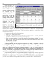
1.3
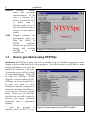
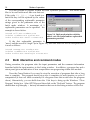
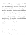
Figure 1.1. NTSYSpc main window
How to get started using NTSYSpc
Installation of NTSYSpc is quite easy since a standard type of installation program is used.
Simply insert the disk and run its setup program. The only decision you will have to make
during installation is to select the
name of the directory to be used.
A program group will be created
on your startup menu. There will
be icons for NTSYSpc, NTedit,
help files, and the readme.txt file.
NTSYSpc can be un-installed (e.g.,
in case you need to move
NTSYSpc to another computer) by
using the standard Add/Remove
icon from the Windows Control
Panel. When you run NTSYSpc
the first time you will be asked to
provide your name, institution
(optional), and a registration
number.
Once
the
program
is
installed, click on the NTSYSpc
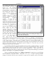
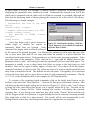
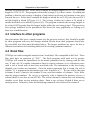
Figure 1.2. Entry form for the OUTPUT module.
Introduction
7
icon in the start menu to see
what NTSYSpc "looks like" (see
Figure 1.1).
The NTSYSpc
main window is divided into
several regions. At the left is a
bar divided into folders with
each containing buttons for
several
computational
modules. Click on a button
(such as “Output”) to load the
corresponding
program
module.
A form will be
displayed in which you can
specify the input file and other
options for the selected module
(see Figure 1.2). A test data set,
TEST.NTS, is supplied so you
can try a few operations right
away. Click on the cell
opposite “Input file” to bring
up a file open dialog box. Note
that by default the dialog box
assumes that data file names
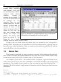
end with the file extension Figure 1.3. Listing window after running the Output module
“.NTS”. For other types of on the TEST.NTS data file.
files,
click on the “File of
type:” window at the lower left and select “Excel”, “Nexus”, or “All files.” Use this dialog to
locate the TEST.NTS file in C:\NTSYS (or wherever you installed NTSYSpc) and then click
on the “Open” button. Then click on the “Compute” button to run the Output module. The
results will be displayed in the Listing window (every time you run a module a new section is
added to the listing notebook). An example is given in Figure 1.3. Press the 1 key or use the
Help menu items to open the help file.
You should note that the separate modules do not provide a complete analysis. You will
normally use a sequence of modules in order to carry out a complete analysis. This structure
makes NTSYSpc more flexible and useful in research applications. Unless batch files are
used, this approach also helps one appreciate the various components making up a standard
analysis. See Chaper 7 for a number of examples.
Next, you should read Chapter 2 on “Modes of operation” to learn how to use NTSYSpc
in both interactive and batch modes. Note that This Style of type is used to indicate
strings of characters that the user is expected to type into the computer, such as file names.
8
Introduction
Chapter 4 on “Preparation of input data files” is, of course, essential reading as it describes
the format of the data files. It also describes the use of the special
Be sure to check the README.TXT file for any last-minute notes or corrections to this
User Guide. The blue registration card should also be filled-out and returned since this
allows us to notify you of any problems that are discovered with this version of NTSYSpc. It
will also allow us to notify you of the availability of updates as new programs and features
are added to NTSYSpc. Your comments, corrections, and suggestions about the program are
welcomed.
1.4
What’s new in version 2.1?
Changes to the user interface:
• The design of the user interface has been changed to make NTSYSpc easier to use.
The computational modules are now organized in folders in a bar along the left
side of the main window.
• A customize option allows the user to place frequently used modules in a user
defined folder.
• Excel data files can now be read directly by all appropriate NTSYSpc modules (the
less reliable DDE and OLE methods are no longer used).
• Nexus tree files can now be read and the NTS file format has been extended to
allow trees with OTUs at different heights.
• Plot options (choice of fonts, colors, etc.) can now be saved and reloaded in
graphics options files. The options are now organized in a convenient tabbed
notebook display.
New modules:
• PROCRUSTES – Procrustes superimposition of coordinates of 2D or 3D landmarks
on specimens or superimpositions of multivariate ordinations of any dimension.
• PROCPLOT – 2D and 3D plot of the results of a Procrustes superimposition.
• FOURPLOT – Plot outlines and estimated outlines from the FOURIER module.
• MULREG – generalized multivariate multiple regression. Can be used to perform
simple bivariate regression, multiple regression, multivariate regression, and
generalized least-squares regression (as used for the comparative method).
• PLOT – Plot one or more columns of a rectangular matrix against a selected
column. Points can be given different symbols and connected by lines.
Improved modules
• CONSEN – Input trees can be in the nexus file format.
Introduction
9
• COPH – Input tree can be in the nexus format. Path length (additive) distances
and Phylogenetic covariances can be computed in addition to the usual
ultrametric distances.
• CVA – Can now compute canonical variates scores for individual observations.
• FOURIER – Many changes were made to make this module more useful. Linked
to the new FOURPLOT module for direct viewing of the results.
• MOD3D – Rewritten to provide interactive 3D rotation (drag with the mouse) and
better axis labeling. Different symbols can be given to different points. 3D biplots
can be produced.
• MXCOMP – The Smouse-Long-Sokal 3-way Mantel test has been added along
with the additional plots it requires.
• MXPLOT – Points can be given different symbols. 2D biplots can be produced.
• NJOIN – Completely rewritten to greatly increase its speed. Large datasets (more
than 500 OTUs) can now be processed. Results can be saved in nexus format or as
an extended NTS tree format that allows for unequal heights of the OTUs in the
tree. An option has been added for unweighted neighbor-joining trees.
• OUTPUT – Supports Excel files and the new tree formats.
• POOLVC – Allows missing values in data when computing the mean and
covariance matrices.
• TPSWTS – For convenience, it now includes the Procrustes superimposition step.
It also now provides an estimate of the uniform component for 3D data.
• TREE – Can now plot trees with unequal heights of the OTUs.
NTedit:
• Can now directly read rectangular matrices from Excel files (the DDE and OLE
methods are no longer used).
• A new text-mode display allows NTedit to be used to edit any ASCII file
(including NTSYSpc batch command files). Files sizes up to 16MB with line
lengths up to 32K can be edited. Standard cut, copy, paste, and other text editing
commands are supported.
• The current matrix or file being edited can now be printed from within the editor.
1.5
What was new in version 2.0?
The old DOS program was converted to Windows. There were, of course, major changes
in the user interface was new, but the way in which the program was used was preserved.
Some of the major changes are listed below.
10
Introduction
• The entry forms have been simplified and the listing results are saved to a Listing
notebook window where you can save, delete, or edit the results. You can also cut
and paste them into other software.
• Input file formats: there is no longer a length restriction to the input lines (they were
limited to just 255 characters). Long names permit more descriptive identifiers —
often very important in more complicated analyses involving many files.
• A new NTedit program replaces the previous NTEDITOR program. The new
program recognizes the various file formats and displays files in a spreadsheet-like
grid.
• Graphics: Can now call up the appropriate graphics modules directly from many of
the computational modules. The entry forms for the graphics programs have also
been simplified since the graphic options are now available from option dialog boxes
brought up by clicking on a plot with the right mouse button. You can now control
the colors, fonts, line widths, etc. of most aspects of the plots.
• Batch files have been changed to allow both longer lines and the ability to have
continuation lines for a command. The program now requires that the start of each
command begin with an “*”.
• The information in the previous User Manual has been divided into this User Guide
and the very extensive help file. The help file contains the detailed technical
descriptions of each computational module. Sections can be printed from the help
file if you want the information in a printed form. This User Guide contains only
general information about how to use the program.
The changes to individual modules have been relatively minor since so much effort was
spent simply converting the DOS program to a Windows program.
2. Modes of operation
There are two modes in which NTSYSpc can be used: interactive and batch. In interactive
mode a module is selected from the main window by clicking on a button which causes a
window showing the various parameters and options for that module to be displayed. After
this form is filled in, click the Compute button to “run” the module and have the results
appear as a new section in the Listing window. You start batch mode by selecting the “Run
batch file…” item on the File menu or by using the convenient speed button on the toolbar.
The batch dialog box will let you select a file containing a sequence of NTSYSpc commands,
specify up to nine parameters, and run the batch file. The batch file contains commands that
call up various modules, supply parameters, and execute them automatically. Batch files are
Modes of operation
11
convenient for the processing of large data sets or for processing a large number of data sets
(perhaps from a simulation).
2.1
Interactive mode
The main program window displays a program bar with folders corresponding to sets of
program modules (see Figure 1.1 above).
Click on a folder to select a section. This displays buttons corresponding to the modules
available from that section. To select a module, click on the corresponding button. The
selected module will then display a parameter entry form at the right side of the main
program window (such as that for the STAND program shown in Figure 2.1). To run a
program you must enter the required infor mation in the Entry Window (you need to at least
specify the name of an input file). To fill in the entry form, select the desired locations in the
form using a mouse and enter the appropriate information (the method of entering the
information depends on the type of field). The default choices, if there are any, will have
already been entered into the form.
Input or output matrix names: names are any valid Windows file names (including long
names). File names can, optionally, be preceded by a drive specification (e.g.,
a:test.nts) or a path specification (e.g., c:\data\test.nts). If the name
contains either a colon or a backslash character, then the name is used as is.
Otherwise the name will be appended to the current data directory. The program
will remember the drive and directory from previous runs so that you do not have
to enter it every time if all the files are in the same directory. It is easiest to simply
double click on the cell to bring up a file open dialog box where you can select the
file visually.
Numerical constants: Often numerical constants make sense only within certain limits.
NTSYSpc will not permit you to enter an out-of-range value. Decimal points should
not be typed when integer numbers are expected by the program.
Pick lists: Many of the programs require one to select one of several choices for a field (such
as a method of standardization or a clustering method). They are indicated by the
small upside down triangle at the right end of the field (there are two examples in
Figure 2.1). Click on the field to display a list of the available choices. Move the
cursor or the mouse to high-light the desired option and then click with the left
mouse button. Sometimes there is a blank entry signifying that this option is to be
ignored. The selected code will then be entered into the form.
12
Modes of operation
Checkboxes: Press the space bar
or click with the mouse
to alternate between
checked (for yes) and
unchecked (for no)
states. These are used
to indicate, for example,
whether the program
should operate on the
rows of the input
matrix
or
whether
additional information
should be included in
the output listing.
Once the fields have been
filled--in correctly, click the Figure 2.1. Dialog window for the STAND module.
Compute button to run the
program (since the Compute button has the focus initially, you can also just press the R key).
The Listing window will be opened to a new section and it will show a summary of the input
parameters you specified, information about the input files, and the results of the
computations. If you provided names for output files then these results are stored on disk
and are available as input to other modules. For some programs short-cut graphics speed
buttons will appear on the small toolbar at the bottom left of the parameter entry window.
Pass the mouse over the button to display the hint box describing the type of plot produced
by each button. For example, Figure 2.2 shows the buttons available after running the EIGEN
program.
In case of an error (such as entering the name of a non-existent file for an input data
matrix), the program will "beep" and display a message in an Error Window. Click the OK
button to close this window so that you may
correct the problem and try again.
To close the parameter entry window for
a module you may either click the Close
button or simply select another module from
the NTSYSpc main window.
2.2
Batch mode
Figure 2.2. Graphic speed buttons for the
EIGEN module. The first button calls
MXPLOT to produce a 2D plot of the
eigenvectors and the second calls MOD3D
for a 3D plot.
Modes of operation
13
In batch mode NTSYSpc will attempt to directly execute a sequence of modules without
displaying the parameter entry windows for each. Commands are entered in an ASCII file
which can be prepared with an editor such as Windows notepad or wordpad (although the
latter has the annoying habit of always placing the extension .txt at the end of a file name).
The following is a simple example.
' standardize the rows of the data
matrix
*stand o=data r=sdata
' compute distances among the OTUs
*simint o=sdata r=dist
' now perform a UPGMA cluster
analysis
*sahn o=dist
r=tree
Lines that begin with a quote characters
Figure 2.3. Batch mode window. Click the
(either single or double) are treated as "Load" button to select a batch file and then
comments. Blank lines are ignored.
Each click the "Run" button.
command line begins with an asterisk followed
by the name of the desired program. It is followed by parameter=value pairs that may take
one or more lines (lines that do not start with either an asterisk or a quote character are
considered continuation lines). Each parameter is a code for some program parameter. Value
gives the value of the parameter. There must be an "=" sign (and no blanks) between the
parameter and its value. Each such pair must be separated by at least one blank space. The
parameter is usually a one to three letter code (they are given in the help topic for each
module). They can be typed in either upper or lower case. The values can be file names,
numerical constants, or option codes. The values are identical to what would be specified in an
entry form in interactive mode. The defaults are also the same. For legibility it is convenient
to keep the lines short and use more than one line for each command if convenient. The file
TEST.NTB on the distribution disk is an example of a NTSYSpc batch file.
To execute a file containing batch commands, click on the batch speed button on the
toolbar or else select the “Run batch file…” item on the File menu of the main window. This
will bring up the batch mode dialog box as shown in Figure 2.3. Click on the “Load” button
to bring up a file open dialog that allows you to specify which file to use. The click on the
“Run” button to execute the file. While running, this window will display the currently
executing line. If you change your mind you may click on the “Cancel” button and the run
will be stopped at the next iteration or logical breakpoint in the currently executing module
(this might take a while for a large matrix). The results will be sent automatically to the
Listing window where they can be inspected when the computations are complete.
14
Modes of operation
It is also possible to prepare a batch file with replaceable parameters. This allows batch
files to be used with more than one data set.
If the codes %1, %2,…, %9 are found in a
batch file they will be replaced by the values
of the corresponding replaceable parameter
strings given in the parameter area of the
batch mode window. A maximum of 9
replaceable parameters can be specified. An
example is shown below.
*stand o=%1.nts r=sdata.nts
*simint o=sdata.nts r=dist.nts
*sahn o=dist.nts cm=%2 r=tree.nts
Figure 2.4. Batch mode window with the
test2.ntb file loaded and two replaceable
parameters provided.
If the first replaceable parameter is
"mosq" and the second is "single" (as in Figure 2.4), then this batch file will be interpreted as if
it were as follows:
*stand o=mosq.nts r=sdata.nts
*simint o=sdata.nts r=dist.nts
*sahn o=dist.nts cm=single r=tree.nts
2.3
Both interactive and command modes
During execution, the programs echo the input parameters and the comment information
furnished with the input matrices to the Listing window. In addition, a progress bar and a
status panel given an indication of how computations are progressing within each module.
Press the Cancel button if you need to stop the execution of programs that take a long
time to complete. The program should stop once it completes its next iteration or cycle of
computation (it does not check constantly for a keypress since that would slow the program
down). Alternatively, you can hold down the CAD keys to bring up the Windows “Close
Program” dialog box. Select NTSYSpc and then click on the “End task” button. The program
should then stop abruptly — but any information that was in the listing window will be lost.
Menus & related windows
15
3. Menus & related windows
3.1 Main menu
Across the top of the main window is a menu bar (see Figure 1.1). The various choices are
described below.
File
This pulls down a submenu from which you can select “Edit data file,” “View
listing,” “Printer setup,” “Run batch file,” and “Exit.” The edit menu item displays
a file open dialog in which you can specify the name of the NTSYSpc file you wish
to edit. The separate program NTedit (included with NTSYSpc) is then run. If the
file is a valid NTSYSpc file then it will be displayed in a spreadsheet like format. If
there are any errors in reading the file then an alternative ASCII editor (such as the
Windows notepad or some other user selectable editor) will be run. The view listing
item opens the Listing window (see Section 3.4). The printer setup item opens the
standard Windows printer setup dialog box. The run batch file item brings up the
Batch mode dialog box so that a batch file can be run (see Section 2.2). The exit item
closes the program (the program can also be closed by clicking on the Close speed
button on the tool bar.
Options This pulls down a submenu from which you can select “Configuration” or “Restore
defaults.” The configuration item will display a parameter entry form for various
program configuration options.
The restore defaults item will reset the
configuration parameters back to their original states. The “Customize” option will
allow you to add or remove modules from the User folder. See the examples in the
next two sections.
Help
This pulls down a submenu from which you can select “Contents,” “Topic search,”
or “About.” The contents item displays the table of contents for the help file. Topic
search brings up the Help topics dialog box in which you can search for various
terms. The about item displays the NTSYSpc about box showing copyright
information, version number, and the registration number.
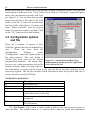
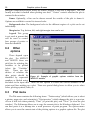
3.2 Customization options
16
Menus & related windows
Because most analyses require one to run modules located in different folders, you may find
it convenient to make use of the “User” folder. If you click on “Customize” under the Option
menu, the customization module will load
(see Figure 3.1). You can then drag module
names from the list at the right to the User
folder on the left. To remove a module from
the User folder right-click on its name and
select “Remove module” from the pop-up
menu. You can also rename a module. Click
on the “OK” button to close this window.
3.3 Configuration options
and file
There are a number of aspects of how
NTSYSpc operates that can be modified by a
user.
These are done from the
Configuration
Window
(select
“Configuration” under the Option menu on
the main window). This will display a
window like those used for the various Figure 3.1. Customization window. Drag
computational modules. The entries here, module names from the list at the right to the
however, are system parameters such as file User folder at the left.
formats, directory names, and other options.
The information you enter will be saved in the ntsys.ini file in the same directory as the
ntsys.exe program. The file also includes coded information about the position and size of
various windows used by NTSYSpc.
Configuration parameters
Batch code
FF
LF
LI
DD
OW
ED
Description
File format code.
Listing format code.
Listing indent when printing.
Data directory—the directory to use as the
current directory for data files.
File overwrite code. ?=ask, O=overwrite, and
A=append.
Editor to be called from the toolbar or the
File|Edit menu.
The “File format” code is used to write results to disk so they can be used as input to
other modules. The default format of “e” ensures these values are saved with maximum
Menus & related windows
17
precision. This value should not be changed except possibly when working with very large
matrices and you are low on disk space. On the other hand, the “Listing format” code will
often be changed so that numerical information displayed in the Listing window has an
appropriate level of precision for a given data set. The default is “8.4f” which means that
floating-point numbers should be displayed with four decimal places within a field eight
characters wide. You can also enter the code as “F8.4” as in FORTRAN but the NTSYSpc will
always store the code with the “f” at the end.
The “File overwrite code” is used to determine what should happen when the program
attempts to save a data file with the same name as an existing file. Ask means that a window
will pop-up asking what should be done, overwrite means that the existing file should be
deleted, and append means that the new file will be appended to the end of the existing file.
If you wish, another editor can be substituted for the NTedit program.
Note: the configuration parameters can also be changed through commands in a batch
file. Use CONFIG as if it were a module and use the "batch codes" given above to change the
values of the parameters. as the following:
config LF=9.6f
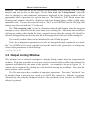
3.4 Output Listing Window
This window uses a notebook metaphor to display listing output from the computational
modules. Each time a module is run a new section is created with an index tab numbered in
sequence and labeled by the name of the module. An example is shown in Figure 3.1. A
section can be examined by clicking on a tab and then moving the scrollbars. Note that the
entire window can be resized.
The File menu provides a number of important operations. The entire “notebook” can
be reloaded from a previous run, saved to an ASCII file, cleared (i.e., deleted), or printed.
Alternatively, the currently displayed section of the notebook can be saved to an ASCII file,
deleted, or printed.
18
Menus & related windows
The Edit menu provides commands to select all the text in the current section, to cut
selected text to the Windows clipboard, to copy selected text to the clipboard, and to paste in
text from the clipboard.
These commands permit
you to copy results into
other software such as a
wordprocessor. They also
allow
you
to
delete
unwanted
information
before printing or saving to
a disk file. Keeping such
notebooks is a convenient
way to verify which options
were used to produce a
certain result. The purpose
of reloading a notebook is
to allow the appending of
new results so that a record
of all the computations for a
particular project can be
kept together.
The file
format is simply an ASCII
file with the form feed
character
separating Figure 3.2. Example of the listing window after running the
commands in the test.ntb batch file.
sections.
The Options menu
allows you to change the font used both for the on-screen display and for printing. The
indent item controls the size of the left margin when printing.
The Help menu provides the standard contents, topic search, and about items.
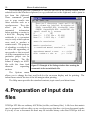
4. Preparation of input data
files
NTSYSpc NTS files are ordinary ASCII files (txt files, not binary files). A file for a data matrix
may be prepared with an editor or any word processor that has a txt (non-document) mode.
If you try to use a document file there may be invisible binary codes that NTSYSpc will not
Preparation of input data files
19
know how to interpret. Free-format is used for the entries in the data matrices. This means
that at least one blank space or a comma is required between numbers. The NTedit program
included with NTSYSpc can be used to prepare data files and ensure that they are in the
proper format. In addition, NTSYSpc can also read data matrices from Excel spreadsheets
(*.XLS files) and trees from Nexus format files.
4.1 NTS file formats
A matrix can contain 4 kinds of records. The comment and label lines are optional.
Comments These optional lines are used to include notes with the data. The first character in
each line must be some type of quote character " or '. The infor mation on these lines
will be copied onto comment lines in any matrices based on this input matrix. In
addition, each subsequent program will add an additional comment line so that the
sequence of steps leading to a given matrix can be determined.
Matrix parameter line This line contains 4 integer numbers (The second and third may have a
suffix letter to indicate the presence and location of row and column labels) and
possibly a floating point number. They must be separated by at least one blank
space.
•
•
The first number is a code for the type of matrix.
1
rectangular data matrix,
2
symmetric dissimilarity matrix,
3
symmetric similarity matrix,
4
diagonal matrix,
5
tree matrix for dissimilarity data,
6
tree matrix for similarity data,
7
graph matrix for dissimilarity data, and
8
graph matrix for similarity data.
The second and third numbers are the numbers of rows and columns in the matrix.
If labels are to be furnished for either the rows or columns (or both) then a letter
must be entered right after the number (with no spaces in between). An “L” is used
to indicate the presence of a list of labels in a separate record placed before the data.
For example, “25L” means that there are 25 rows and labels are furnished in a
separate record. A lower case "l" can also be used—but this is less desirable since it
looks so similar to the number "1". The letter “B” is used to indicate that row labels
are placed as the first item in each row and “E” indicates that the row labels are
placed after the end of each row.
20
Preparation of input data files
•
The fourth number is 0 if there are no missing data in the matrix. If there are
missing data then the fourth number should be a "1" followed by at least one blank
and then the numerical code used to denote the missing values—999 is a popular
choice.
Row and column labels Labels must be furnished if a "B", "E", or "L" is placed after the
numbers of rows or and "L" after the number of columns in the previous line. Row
labels can be placed in one of three locations: as the first element at the beginning of
each row (B), as the last element at the end of each row (E), or as a separate list of
row labels in front of the matrix (L). The column labels if present always consist of a
list of labels with the first label beginning on a new line. Each label consists of
strings of characters (up to 16 letters or digits but no blanks). They are separated by
one or more blanks or by a comma, i.e., the are entered free format. Examples are
given below.
Matrix data lines The elements of the matrix are entered with rows in the input matrix
corresponding to one or more lines in the input file (i.e., matrices are always entered
rowwise). Symmetric matrices are entered as rows beginning with column 1 and
ending with the diagonal elements (i.e., the lower half matrix with diagonals is
entered rowwise). If all the elements for a row do not fit on a single line, then
continue typing on as many new lines as needed. It is impor tant that the first
element of a new row starts on a new line—even if the previous line is mostly
empty. The elements themselves are free format. Values must be separated by one
or more blanks or a comma. Missing values are indicated by the numerical code
provided on the matrix parameter line. They cannot be simple left blank (they can,
however, be indicated by a “.” if a missing value code is provided on the matrix
parameter line).
The lines can be very long (the theoretical limit is 2 GB!)—but it will be easier to work
with them with most editors if you use shorter lines (80 characters or fewer). Blank lines are
ignored.
More than one matrix can be stored in a single file. The records for a second matrix
(starting with the optional comment lines) simply follow after those for the first. Most
program modules in NTSYSpc will perform the selected set of operations on each of the
matrices in an input file. The results for the second and subsequent matrices are simply
appended to the files produced by processing the first matrix. For some programs it is
necessary to put more than one matrix in a single file in order to perform a certain
computation. It is required by programs such as CPCA, CVA, and POOLVCV. It is also
necessary in order to compute the majority rule consensus tree for more than two trees.
Note: if you prepare the original data matrix so that the rows correspond to the
characters (variables) and the columns correspond to the objects being classified (OTUs, data
points, etc.), then you will find that many of the default row/column direction options will be
correct.
Preparation of input data files
21
Because there is always the chance that there will be an error in the preparation of a data
matrix, it is strongly suggested that you use the NTedit program and that you first try the
OUTPUT module to display your input data matrix. It can be printed out for convenience in
proofing. If there are major problems in the file format you may need to load the matrix into
NTedit in text mode.
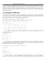
4.2 Examples of NTS files
An example of a data matrix file with 3 comment lines and labels for the columns but not the
rows is given below. This set of test data is furnished on the distribution disks for NTSYSpc
and is used for many of the examples given in this manual.
"A sample data matrix to test NTSYSpc
"There are 5 characters (rows) and 10 OTUs (columns)
"The columns are labeled. No missing values.
1 5 10L 0
A B C D E F G H I J
8
7
9 13
6 12
9
7 11 6
5
6
3
3
7
10 5
7
5 7
11 13 12
9
8 18 17 21 22 13
10 18 22
8
7 17 18 26 24 18
11
6 12 10 10 19 13 13 19 14
An example of a data matrix with column labels and with row labels placed at the
beginning of each row:
1 4B 3L
c1 c2
r1 1,
r2 3,
r3 3,
r4 2,
0
c3
3,
2,
4,
1,
4
1
2
2
An example of a symmetrical correlation matrix file (note that elements past the
diagonal of a symmetric matrix must not be entered). Labels can only be placed in a list in
front of the data (i.e., only the “L” code is valid).
"A sample correlation matrix with labels
3 5L 5 0
A B C F E
1
0.4 1
0.3 0.4 1
0.6 0.3 0.4 1
0.7 0.3 0.4 0.5 1
In this case the “L” can be appended to either the number of rows, the number of
columns, or to both. But only one set of labels should be furnished. If a symmetric matrix is
22
Preparation of input data files
the output of some other program it may be stored as a full square matrix. In that case you
should code it as a rectangular matrix and use the SYMD or SYMS options of the TRANSF
program to convert it to the lower half matrix form required by NTSYSpc.
Tree matrices (matrix types 5 and 6) are usually produced by programs rather than
entered by a user. The usual exception is when one wishes to enter an expected tree to
compare with the observed results (using the CONSEN program). There are two styles in
which a tree can be entered in NTSYSpc. The format used internally in NTSYSpc is described
at the end of the description of the SAHN program.
In addition, you can describe a tree using nested parentheses as in the NEXUS format
used, for example, in the program PAUP. This option is only available for tree matrices based
on dissimilarities (matrix type code = 5). While complete NEXUS files cannot be read, the
tree descriptions can be processed as long as the OTUs names are given as integer numbers
(corresponding to their position in a data matrix). This format is provided to enable trees
produced by other programs to be entered into NTSYSpc more easily. One can also enter
trees by hand using this notation -- but it becomes awkward for large trees since it is easy to
miscount parentheses.
In this format nesting is indicated by parentheses, branch lengths (which are optional)
are given in the format ":value" after each OTU name and right parenthesis, and the end of
the tree is indicated by a semicolon. If branch lengths are not provided then NTSYSpc will
generate arbitrary clustering levels consistent with the set relationships given in the tree.
Note that one must either provide branch lengths for all branches or else for none of them. A
mixture will produce unpredictable results.
Example of a NEXUS style tree not using branch lengths:
" NEXUS style input with OTU labels provided.
5 5L 2 0
A B C D E
(((1,3),2),(4,5));
This implies a tree of the following topology:
1--.
3----.
2----L---.
4--.
|
5--L-----L--Example of an input file using branch lengths:
" Example using branch lengths but no OTU labels.
5 5 2 0
(((1:2.1,3:2.5):1.6,2:3.3):0.7,(4:0.5,5:0.3):0.9);
This tree has the same topology as in the previous example. It should be noted, as in the
above example, that the branch lengths may be inconsistent with the levels (heights) used to
Preparation of input data files
23
describe an ultrametric tree. In the above example the branch length for OTU 1 is 2.1 but the
length for OTU 3 is 2.5. The program will use the average (2.4) of these values. An additional
problem is that the raw average of heights of each interior node may not increase as one goes
towards the root. In the above example the height at which the set {1,3,2} joins the root is 4.3
and the height at which {4,5} joins is 1.3. The average of these two values is 2.8 which is
smaller than the level at which {2} joined {1,3}. The program constrains the average heights to
be at least 0.0001 greater than the largest height within the sets being joined. This preserves
the topology indicated by the parentheses but shows the trees graphically as looking as if
there was a multifurcation.
4.3 Interface to other programs
Since the matrix files have a simple format (see the previous section), they should be usable
by other programs with very few changes needed. Results from other programs should also
be convertible into the format described above. The largest problems are apt to be due to
different conventions for furnishing labels and for reading symmetric matrices.
4.4 Excel files
NTSYSpc can read rectangular matrices from "worksheet" files compatible with Excel. These
files must have an extension of “XLS.” The Excel program itself need not be present.
NTSYSpc will search the spreadsheet for the matrix parameter line by starting with the first
row. If only cell A1 contains information then its search continues on to subsequent rows
until a row is found with at least four non-blank cells. The information in the rows being
skipped over is taken as comments. Once the matrix parameter line is found, the cell in
column “A” is interpreted as the matrix type code. It must be a "1". The two cells to the right
(columns B and C) must be the number of rows and the number of columns. Note: these
must be integer numbers. Do not try to append a code to indicate the presence of row or
column labels as one does for an NTS file. The cell in column D contains the code indicating
whether or not there are any missing values. Enter a zero or leave it blank if there are no
missing values. Otherwise, enter the identifying numerical code in the cell in column E.
24
Preparation of input data files
The next row contains
column labels beginning
with column B. If any cells
are left blank they will be
replaced
with
column
numbers.
Column A
contains the row labels. If
any cells are blank then will
be
replaced
by
row
numbers. Thus row and
column labels are in their
natural position—not as
records in front of the
matrix as in as in the “L”
option for NTS files. The
row and column labels
should not contain any Figure 4.1. Example of a sample data file in Excel. Note that the
blanks. The matrix itself first two lines are actually text in cells A1 and A2.
begins in column B. See
Figure 4.1 for a simple
example where the matrix starts in cell B5.
If empty cells are found within the matrix, they are assumed to also correspond to
missing values. Information in the spreadsheet in rows beyond the matrix is ignored and can
be used to store other information. Only one matrix can be read from each Excel file and the
matrix should be in the first spreadsheet .
1.6
Nexus files
This format is supported by many programs concerned with estimating phylogenetic
trees. Within NTSYSpc, the NJOIN module can save tree files in this format. Trees in this
format can be read by the COPH, CONSEN, and OUTPUT modules.
An example is given below. The translate section is required. It gives the labels for the
OTUs. There can be one or more tree commands in a file. Each describes a tree using nested
parentheses. The length of each branch on the tree must be provided following the “:”
character. The file is treated a single stream of characters with line breaks provided wherever
convenient.
#nexus
begin trees;
[11 mosq. extracted from Harbach & Kitching (1998)]
translate 1 Anoph1, 2 Toxo12, 3 Wyeo13, 4 Uran17, 5 Culi21, 6 Orth28,
Preparation of input data files
25
7 Mans29, 8 Psor32, 9 Aede44, 10 Cule101, 11 Dein126;
tree (1:16,(4:2,((6:1,(5:1,2:1):3):3,
((9:1,(8:1,7:6):4):2,((10:1,11:3):1,3:30):1):2):2):8);
end;
The nexus file format is described in: Maddison et al. (1997). The method used for
describing trees is called the “Newick Standard” and was adopted June 26, 1986 by an
informal committee meeting during the Society for the Study of Evolution meetings in
Durham, New Hampshire. James Archie, William H.E. Day, Wayne Maddison, Christopher
Meacham, F. James Rohlf, David Swofford, and Joe Felsenstein were present. The reason for
the name is that the second and final session of the committee met at Newick's restaurant in
Dover, NH. Examples and a simple description of this format are available at
http://evolution.genetics.washington.edu/phylip/newicktree.html.
5. NTedit
The Ntedit program, included with NTSYSpc, is a data editor designed for use with
NTSYSpc data files. For each of the basic file formats (rectangular, symmetric, diagonal, tree,
and graph) it displays an appropriate arrangement of the cells in the spreadsheet. Using
NTedit ensures that the files are formatted correctly.
The program can be started in three ways.
1. Click on the NTedit icon to start the program.
2. Load this program from the File|Edit file data file menu item or the edit speedbutton on NTSYSpc’s toolbar.
3. Use a DOS command window and type ntedit and the name of a file and then press
the R key to start the program.
Once the program is started, you can either create a new file or load an existing file. NTS
format files can be loaded either in a spreadsheet like grid (Figure 5.1) or in a plain ASCII text
editing (Figure 5.2) view. Excel files can only be displayed in the grid view and nexus files
can only be displayed in the text view.
26
NTedit
In the grid mode you
can enter or correct data in
any of the cells. You can
insert or delete rows and
columns within the table
by
clicking
on
the
appropriate menu choices
or the speed buttons on
the tool bar. You can also
add or delete rows and
columns from the end of
the table by entering new
values in the edit boxes
displaying the current
numbers of rows and
columns. To change the
labels for the rows or Figure 5.1. Example of NTedit with the test.nts file loaded in a
columns (given in the first, grid view.
protected, row or column of the data table) click on the RowLabs or Col.Labs buttons to
unprotect these entries. You can then type new information in these cells. The new names
must not have any blanks within them. Click these buttons again to re-protect these labels
from accidental change.
To create a new file use the following steps:
1. select “New” from the file menu,
2. select the proper matrix type from the list (you may receive a warning about the
possible loss of data when you change matrix types),
3. enter the correct numbers of rows and columns in the edit boxes labeled “No. rows”
and “No. cols.” (note that the new values do not take effect until your cursor leaves
the edit boxes), and then
4. start entering your data.
If there are missing data the identifying numerical code needs to be entered in the edit
box labeled “Missing.” Click on the “Comments” button if you wish to add comments to the
matrix. When you are done you can use the “Check matrix” item under the Edit menu to
check that all data values are properly formatted numbers. It also will check to make sure
there are no empty cells. This same check is made when to attempt to save the matrix to a
disk file. You will be given a chance to replace all the empty cells with whatever code you
specified for missing data (if that field is blank then zeroes will be used).
NTedit can also be used to view and make changes in existing files. Changes have to be
made with care as there is no “undo” feature. A limitation of this mode is that the file must
already be in a proper format. If you try to load an NTS file that is not formatted properly
you will receive an error message and NTedit will try to load the file in ASCII text mode.
Preparation of input data files
27
More flexibility is
provided when editing a
file in ASCII text mode
(see Figure 5.2). Text may
be freely moved around
and cut and pasted from
other software. An “undo”
and “redo” feature is
implemented (see the Edit
menu).
The NTedit help can
be consulted for additional
information – including
various
keyboard
shortcuts.
Figure 5.2. Example of NTedit with the test.nts file loaded in
ASCII text mode.
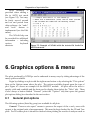
6. Graphics options & menu
The plots produced by NTSYSpc can be enhanced in many ways by taking advantage of the
many options available.
Begin by clicking on a plot with the right mouse button or by selecting the “Plot options”
item on the Options menu above the plot. The options available depend upon the type of
plot. Figure 6.1 shows an example for the MXPLOT module. All plots allow the user to
specify a title and a subtitle and the fonts used to display them (select the “Titles” tab). There
is also always a button labeled “General” (select the “Options” tab) that opens the general
plot options dialog box described in the next section.
6.1
General plot options
The following options (listed by group) are available for all plots.
General: “Preserve axis aspect” means to preserve the aspect of the x and y axes with
respect to the original units of measurements. This must be kept checked for the 3D and Tree
plots. For 2D scatter plots it should be checked when plotting the results of analyses such as
28
Graphics options & menu
principal components analysis where the relative lengths of the axes is important. One will
usually not want it checked when plotting raw data. “Center” controls whether the plot is
centered in the window.
Frame: Optionally, a line can be drawn around the outside of the plot to frame it.
Options are available to control its size and color.
Background color: The background color in the different regions of a plot can be set
individually.
Margin size: Top, bottom, left, and right margin sizes can be set.
Legend: This group
is not used at present but
will be used to control
how groups of points or
lines are identified.
6.2
Other
options
These depend upon
the plot. For MXPLOT
and MOD3D there are
pick lists for selecting the
variables to be plotted
(select the “Variables”
tab).
There are also
choices of whether the
data points should be
Figure 6.1. Example of graphic options window from the
identified by sequential MXPLOT module.
numbers or labeled using
the labels in the input data. There are also options to control the various attributes of the
points and lines making up a plot. There are special dialog boxes to allow you to select
colors, plotting symbols, fonts, etc.
6.3
Plot menu
The File menu contains the following items: “Printer setup” (which allows you to select
a printer, paper size, and orientation), “Print preview” (which changes the plot to a preview
of how it will look when printed), “Print” (to print the plot), and “Close” (to close the plot
window). The Edit menu allows one to copy the current plot to the Windows clipboard. You
can then paste it as a bitmap into a word processor or paint program. The options menu
allows you to save the current state of the plotting options to a graphic options file. The plot
Graphics options & menu
29
options (colors, point and line options, etc.) can later be restored by loading this file. The Help
menu leads to the standard Contents, Topic search, and About items.
7. Typical applications
Furnished below are some examples of typical applications of NTSYSpc. For simplicity, the
required steps are shown as sequences of batch command statements. This is a compact way
to describe the sequence of modules and their parameters. See the help file for more detailed
technical information about each module.
Note lines that begin with a quote character are treated as comment lines and are ignored
by NTSYSpc.
7.1
Cluster analysis
Perhaps the most common use of NTSYSpc is for performing various types of agglomerative
cluster analysis of some type of similarity or dissimilarity matrix. The following is an
example of a batch file that will standardize a data matrix, compute distance coefficients
among the columns of the standardized data matrix (there are several other choices of
coefficients), cluster the distance matrix using the single-link clustering method (there are
other choices, such as UPGMA), compute a cophenetic-value (ultrametric) matrix, compute
the cophenetic correlation as a measure of goodness of fit, and then plot the results in the
form of a phenogram. The distance matrix is also displayed.
" Standardize the variables
*stand o=data.nts r=sdata.nts
" Compute a distance matrix
*simint o=sdata.nts r=dist.nts c=dist
" Do a single-link cluster analysis of the distance matrix
*sahn o=dist.nts r=tree.nts cm=single
" Display phenogram
*tree o=tree.nts
" Compute cophenetic values
*coph o=tree.nts r=coph.nts
" Compute the cophenetic correlation
*mxcomp x=coph.nts y=dist.nts
When working interactively, one can view the tree from within the SAHN module by
clicking on the plot speed button. Note that the Mantel test results displayed by the
MXCOMP module should be ignored since the two matrices being compared are not
independently derived.
30
7.2
Typical applications
Ordination analyses and biplots
In ordination analyses the goal is to position points along coordinate axes in a low
dimensional space (rather than to form sets of points as in cluster analysis). There are many
different methods depending upon the criteria used to define what is meant by the “best”
low-dimensional representation of the relationships among the points. Several programs in
NTSYSpc can be used to perform these analyses.
When an original data matrix is available it is possible, and usually desirable, to make
plots of both the variables and the points with respect to the same axes. This is called a
“biplot”. This allows one to not only see the patterns, trends, etc. among the points and of
relationships (usually correlation) among the variables, but also the relationships between the
points and the variables — at least to the extent that they can be summarized in a few
dimensions. Unfortunately, there seems to be no strong consensus about how to scale the
two ordinations relative to one another. Gabriel (1968, 1971, 1981) defines a biplot of an n×p
matrix Y as a simultaneous bivariate plot of the n points in each column of a matrix A and of
the p variables in each column of matrix B, where Y=ABt (it would be a bimodel if a 3dimensional plot were made). Matrices A and B can be expressed in terms of a singularvalue decomposition of matrix Y: Y=UΛVt. One could set A=UΛ and B=V (called a JK biplot
by Gabriel and Odoroff, 1986). In terms of principal components analysis, this corresponds to
computing normalized eigenvectors from the correlation or variance-covariance matrix for
the variables and then using the PROJ program to project the points onto these vectors. The
rows of A are plotted as points and the rows of B are plotted as vectors. Note that the matrix
Λ of singular values is the square root of the eigenvalue matrix obtained in a principal
components analysis. This type of decomposition of a data matrix is called preference scaling
or repertory grid analysis in psychology and sociology.
One can equally well set A=U and B=VΛ (GH biplot of Gabriel and Odoroff, 1986). One
could also multiply both U and V by L 0.5 (an SQ biplot). This latter choice would seem most
appropriate in correspondence analysis where both the rows and columns can be interpreted
as variables The matrix Λ could also be apportioned in any other way to U and V as long as
their product yields Y.
A problem with a JK biplot is that the vectors for the variables are of unit length and
thus are not in the same scale as the vectors for the points. Since the vectors for the variables
are dimensionless a plot of them does not indicate how well the variance of each variable is
explained by the number of dimensions used. For this reason one can deviate from a true
biplot and multiply both U and V by Λ. As a consequence, one cannot visually estimate an
element, say yij, of the original data matrix as simply the inner product of row i of A and row j
of B, one must compute the projection of row i of A onto row j of B. One compares the
relationships between the ordinations of the points and of the variables by examining the
angles between them. Jackson (1991) indicates that this alternative is popular “among French
practitioners.”
Typical applications
31
The MXPLOT module can be used to make a biplot. Enter the name of the matrix giving
the coordinates of the points as the primary input matrix and enter the name of the matrix
giving the coordinates of the variables as the secondary input matrix. The secondary matrix
is plotted at the same scale and shown as vectors from the origin. If the vectors are too short
or too long one may use the TRANSF program to scale them to a more convenient length.
7.3
Principal components analysis
Principal components analysis, PCA, is one of the most important methods of ordination
analysis. It constructs a new set of orthogonal coordinate axes such that the projection of
points onto them have maximum variance in as few dimensions as possible. While defined in
terms of variances and covariances, PCA is often applied to standardized data because the
results are sensitive to the choices of units of measurement and the choice of units is often
arbitrary.
The following batch file will standardize a data matrix by rows, compute a matrix of
correlations among the variables (assumes rows), extract 3 eigenvectors from the correlation
matrix, project the standardized data onto these eigenvectors, and then make a 3-dimensional
plot of the objects. Various matrices are also output to files.
" Standardize variables (rows)
*stand o=data.nts r=sdata.nts
" Compute correlations among variables (rows)
*simint o=sdata.nts c=corr r=corr.nts d=row
" Output the correlation matrix
*output o=corr.nts
" Extract first 3 PCA axes from correlation matrix
*eigen o=corr.nts n=3 r=vect.nts val=val.nts
" Output principal component axes
*output o=vect.nts
" Project objects onto PCA axes
*proj o=sdata.nts d=col f=vect.nts r=proj.nts
" Output projections
*output o=proj.nts
" Display 3D plot of projection of objects
*mod3d o=proj.nts
" Display 3D plot of variables defining the PCA axes
*mod3d o=vect.nts d=col
The last two plots together comprise a three-dimensional biplot (a “bimodel”) for these
data.
An alternative procedure would be to not standardize the data and to use a variancecovariance matrix rather than a correlation matrix in the above steps. In such a case, the
largest weights are given to those variables with the largest variances. This implies that the
variables were measured in comparable units of measurement. This might be appropriate,
for example, for a matrix of log-transformed variables in a conventional (non-geometric)
32
Typical applications
morphometric study (perhaps with means subtracted following Darroch and Mosimann,
1985).
7.4
Principal coordinates analysis, PCOORDA
PCOORDA can be thought of as a computational alternative to PCA. The steps shown below
will give results identical to PCA. One important consideration is that when there are many
fewer points than variables computation time may be much less than for the usual PCA.
The batch file given below performs the following operations: the data matrix is
standardized by variables (rows), a matrix of distances between the objects is computed, the
distance matrix is double-centered, the double-centered matrix is then factored and a plot is
made showing the objects in a 3-dimensional space.
" standardize data if in different units
*stand o=data.nts r=sdata.nts
" Compute distances among objects
*simint o=sdata.nts r=dist.nts
" Double-center the distance matrix
*dcenter o=dist.nts r=dcent.nts
" eigenvectors correspond to projections of objects
*eigen o=dcent.nts n=3 r=proj.nts
*output o=proj.nts
" Display -- Note that direction is "col"
*mod3d o=proj.nts d=col
PCOORDA can also be viewed as a distinct ordination method since it can also be
applied to various types of similarity and dissimilarity matrices - or even to experimentally
determined proximity matrices where there is no original “data matrix.” The computational
steps would then be as follows:
" Double-center the matrix
*dcenter o=dist.nts r=dcent.nts
" Extract eigenvectors
*eigen o=dcent.nts n=3 r=proj.nts
" Output eigenvectors = projections
*output o=proj.nts
" Display -- Note that direction is "col"
*mod3d o=proj.nts d=col
Of course, an arbitrary dissimilarity matrix may not be very compatible with a Euclidean
metric. In such cases many of the eigenvalues may be negative. In performing such an
analysis one hopes that such negative eigenvalues are small and can be ignored.
Typical applications
7.5
33
Nonmetric multidimensional scaling
This method is similar to PCOORDA in that it can be used to represent the relationships
among a set of points in a low dimensional space. The difference is that in non-metric
multidimensional scaling analysis the distances among the points in the final configuration
need only have a monotone relationship to the distances implied by the original data matrix.
This relaxed constraint usually makes it possible to get a much better fit in fewer dimensions
than is possible in PCOORDA.
If possible, one begins with the results of a PCOORDA as an initial configuration since
this usually results in many fewer iterations being necessary in the MDSCALE module.
" Use PCOORDA to obtain an initial configuration
*DCENTER O=dist.nts R=dcent.nts
*EIGEN O=dcent.nts N=2 R=init.nts
" non-metric MDSCALE using initial solution
*MDSCALE O=dist.nts N=2 I=init.nts R=final.nts
" rotate result for ease in viewing
*SIMINT O=final.nts C=varcov R=vcv.nts
*EIGEN O=vcv.nts N=2 R=vect.nts
*PROJ O=final.nts D=row F=vect.nts R=result.nts
" plot the final rotated configuration
*MXPLOT O=result.nts
When viewing the plot be sure to set the option “Preserve axes aspect.” The Procrustes
module can be used to compare the final configuration with another ordination such as the
initial Pcoord solution.
7.6
Burnaby's method for size adjustment
The following batch file shows an example of how the ORTH option of the PROJ program can
be used for Burnaby's method to remove the effect of a vector from a data set. The data are
projected onto the hyperplane orthogonal to the specified vector. In the example given below
the first principal component axis is used as "size”. Other vectors such as the isometric vector
(1,1,...,1) could also be used.
" compute VCV matrix from a data matrix
*simint o=data.nts c=varcov r=vcv.nts d=row
" compute first principal component
*eigen o=vcv.nts n=1 r=pc1.nts
" project data onto hyperplane normal to PC1
*proj o=data.nts f=pc1.nts pt=orth r=bproj.nts
The adjusted data matrix bproj.nts can then be used, for example, to compute a
distance matrix which is then clustered by SAHN. The clusters should then not be influenced
by variation in the original data set that was parallel to the first principal component—which
is often mostly due to size. The first principal component points in the direction in which
34
Typical applications
there is the most variation. If the organisms sampled happen to be about the same size, then
this vector is apt to represent sexual differences, polymorphisms, etc. In many cases it may be
safer to use an a priori defined isometric vector as a size vector (i.e., the vector 1,1,1,1…,1) or
to use the first principal component based only on a carefully selected subset of variables.
The adjusted data matrix could also be used as input for a canonical variates analysis or
for the computation of size-free generalized distances (see the CVA module).
7.7
Analysis of shape using landmark coordinates.
In recent years there has been many new developments in the field of geometric
morphometrics. The PROCRUSTES module has been included to provide these methods for
studies using 2 or 3-dimensional landmark coordinates. The PROCRUSTES module will
optimally superimpose specimens and then output the average (“consensus”) configuration
as well as a transformed set of data in which each specimen has been optimally aligned to the
consensus configuration and thus has the effects of variation in location, orientation, and size
removed. This matrix of aligned coordinates can then used as a matrix of shape variables for
principal components analysis, cluster analysis, canonical variates analysis, etc. One has to be
careful with some analyses because a covariance matrix based on these aligned data will be
singular (there will be 4 zero eigenvalues for 2D data and 7 for 3D data). The CVA program in
NTSYSpc can handle this if one changes the value for the “Cutoff for roots” parameter from
zero to a small number (such as 0.000000001).
The TPSWTS module can be used to eliminate the singularity of the aligned data. It
transforms the aligned coordinates to a matrix of partial warp scores. When the alpha
parameter is set equal to zero (the usual choice), this operation can be viewed as a rotation
followed by a projection to eliminate the redundant dimensions. A PCA of a covariance
matrix for the aligned data and a PCA of a covariance matrix based on the partial warp scores
will yield identical results (except for the presence of zero eigenvalues when analyzing
aligned data).
7.8
Comparison of dis/similarity matrices
Often one wishes to test whether one set of relationships among a set of objects is
independent of another. For example one may wish to test whether the degree of
morphological difference between samples is related to the geographical distances between
the sampled populations (see, for example, Sokal, 1979). A simple way to do this is by the use
of the Mantel test (Mantel, 1967). The test assumes that the two matrices have been obtained
independently—one cannot use it to test two matrices where one has been derived from the
other. The steps given below assume that one already has a matrix of geographical distance,
gdist.nts.
" Compute morphological dissimilarity matrix
*simint o=data.nts c=dist r=mdist.nts d=row
" Compare mdist with gdist, 250 random permutations
Typical applications
35
*mxcomp x=mdist.nts y=gdist.nts np=250
The program can also be used to perform a 3-way Mantel test using the Smouse-LongSokal method. This procedure performs a Mantel test two matrices that have been adjusted
for the effects of regression on a third matrix. It allows one to test for the relationship
between two distance matrices when the effects of a third matrix have been held constant.
While less efficient than a specialized program, one can use the MXCOMP module to
perform spatial autocorrelation analyses. The geographical distance matrix is replaced with a
series of matrices corresponding to different geographical distance classes. In each matrix an
entry is 1 if objects i and j are within the desired distance class and is 0 otherwise. To make a
distance correlogram one simply plots the resulting matrix correlations as a function of
geographical distance. The Mantel test can be used to determine which coefficients are
statistically different from zero.
Bibliography
36
Bibliography
Burnaby, T. P. 1966. Growth-invariant
discriminant functions and generalized
distances. Biometrics, 22:96-110.
Darroch, J. N. and J. E. Mosimann. 1985.
Canonical and principal
components of shape. Biometrika,
72:241-252.
Everitt, B. S. and Dunn, G. 1992. Applied
multivariate data analysis. Oxford
Univ. Press: New York. 304 pp.
Gabriel, K. R. 1968. The biplot graphical
display of matrices with application
to principal component analysis.
Biometrika, 58:453-467.
Gabriel, K. R. 1971. The biplot graphical
display of matrices with applicatin
to principal componenet analysis.
Biometrika, 58:453-467.
Gabriel, K. 1981. Biplot display of
multivariate matrices for inspection
of data and diagnosis. P. 147-173 in
Barnett, V. (ed.) Interpreting
Multivariate Data. John Wiley and
Sons, New York.
Gabriel, K. and Odoroff, C. L. 1986.
Illustrations of model diagnosis by
means of three-dimensional biplots.
Pp. 257-274 in Wegman, E.J. and
DePriest, D.J. (eds.). Statistical
image processing and graphics,
Marcel Dekker, New York.
Gascuel, O. 1997. Concerning the NJ
algorithm and its unweighted
version, UNJ. Pp. 149-170 in B.
Mirkin, F. R. McMorris, F. S.
Roberts, and A. Rzhetsky, eds.
Mathematical hierarchies and
biology. DIMACS series in discrete
mathematics and theoretical
computer science, Vol. American
Mathematical Society, Providence,
R.I.
Gnanadesikan, R. 1977. Methods for
statistical data analysis of
multivariate observations. Wiley.
New York. 311 pp.
Hartigan, J. A. 1975. Clustering
algorithms. Wiley. New York. 351
pp.
Jackson, J. E. 1991. A user’s guide to
principal components. Wiley: New
York. 569 pp.
Maddison, D.R., D.L. Swofford, and W.P.
Maddison. 1997. NEXUS: an
extendible file format for systematic
information. Systematic
Biology,.46: 590-621.
Mantel, N. A. 1967. The detection of
disease clustering and a
generalized regression approach.
Cancer Res., 27:209-220.
Reyment, R. A. 1991. Multidimensional
paleobiology. Pergamon Press:
New York, 377 pp.
Bibliography
Romesburg, H. C. 1984. Cluster analysis
for researchers. Lifetime Learning
Publications. Belmont, California.
334 pp.
Saitou, N. and M. Nei. 1987. The
neighbor-joining method: a new
method for reconstructing
phylogenetic trees. Mol. Biol. Evol.,
4:406-425.
Smouse, P. E., J. C. Long, and R. R. Sokal.
1986. Multiple regression and
correlation extensions of the Mantel
test of matrix correspondence.
Systematic Zoology, 35:627-632.
Sneath, P. H. A. and R. R. Sokal. 1973.
Numerical Taxonomy. Freeman.
San Francisco. 573 pp.
Sokal, R. R. 1979. Testing statistical
significance of geographic variation
patterns. Systematic Zool.,
28:227-231.
Sokal, R. R. and P. H. A. Sneath. 1963.
Principles of Numerical Taxonomy.
Freeman. San Francisco. 359 pp.
Weir, B. S. 1989. Building trees with DNA
sequences. Biometric Bulletin,
6(4):21-23.
37
38
Index
INDEX
association coefficients, 5
axis aspect ratio, 27
Batch mode, 13
bimodel, 30
biplot, 30
Burnaby's method, 33
canonical correlation, 3
canonical vectors analysis, 4
cladistics, 1
Cluster analysis, 29
Common principal components analysis, 3
Configuration window, 16
consensus tree, 3
cophenetic value matrix, 3
Correspondence analysis, 3
elliptic Fourier analysis, 4
Excel, 23
File formats, 19
File overwrite code, 17
Fourier analysis, 4
homogeneity of covariance matrices, 5
Installation, 6
isometric vector, 34
line limit, 20
Mantel test, 4, 35
matrix comments, 26
minimum-length spanning tree, 4
missing data code, 20, 26
multidimensional scaling, 33
multidimensional scaling analysis, 4
neighbor-joining method, 5
NEXUS format, 22
Ordination analysis, 30
Output Listing Window, 17
PCA, 31
PCOORDA, 32
phenetics, 1
preference scaling, 30
Principal components analysis, 31
Principal coordinates analysis, 32
repertory grid analysis, 30
replaceable parameters, 14
single-link, 5
singular-value decomposition, 5
size
adjustment, 33
spatial autocorrelation analyses, 35
thin-plate spline, 6
tree matrix, 22
two-block partial least-squares, 3
ultrametric, 23
ultrametric values, 3
UPGMA, 5
XLS, 23