Download MLwiN MCMC Manual - University of Bristol

MCMC estimation in MLwiN
Version 2.32
by
William J. Browne
Programming by
William J. Browne, Chris Charlton and Jon Rasbash
Updates for later versions by
William J. Browne, Chris Charlton, Mike Kelly and Rebecca Pillinger
Printed 2015
Centre for Multilevel Modelling
University of Bristol
ii
MCMC Estimation in MLwiN version 2.32
© 2015. William J. Browne.
No part of this document may be reproduced or transmitted in any form or by
any means, electronic or mechanical, including photocopying, for any purpose
other than the owner’s personal use, without the prior written permission of
one of the copyright holders.
ISBN: 978-0-903024-99-0
Printed in the United Kingdom
First printing November 2004
Updated for University of Bristol, October 2005, January 2009, July 2009,
August 2011, January 2012, September 2012, August 2014 and January 2015.
Contents
Table of Contents
viii
Acknowledgements
ix
Preface to the 2009, 2011, 2012 and 2014 Editions
xi
1 Introduction to MCMC Estimation and Bayesian Modelling
1.1 Bayesian modelling using Markov Chain Monte Carlo methods
1.2 MCMC methods and Bayesian modelling . . . . . . . . . . . .
1.3 Default prior distributions . . . . . . . . . . . . . . . . . . . .
1.4 MCMC estimation . . . . . . . . . . . . . . . . . . . . . . . .
1.5 Gibbs sampling . . . . . . . . . . . . . . . . . . . . . . . . . .
1.6 Metropolis Hastings sampling . . . . . . . . . . . . . . . . . .
1.7 Running macros to perform Gibbs sampling and Metropolis
Hastings sampling on the simple linear regression model . . .
1.8 Dynamic traces for MCMC . . . . . . . . . . . . . . . . . . . .
1.9 Macro to run a hybrid Metropolis and Gibbs sampling method
for a linear regression example . . . . . . . . . . . . . . . . . .
1.10 MCMC estimation of multilevel models in MLwiN . . . . . . .
Chapter learning outcomes . . . . . . . . . . . . . . . . . . . . . . .
2 Single Level Normal Response Modelling
2.1 Running the Gibbs Sampler . . . . . . . .
2.2 Deviance statistic and the DIC diagnostic
2.3 Adding more predictors . . . . . . . . . . .
2.4 Fitting school effects as fixed parameters .
Chapter learning outcomes . . . . . . . . . . . .
.
.
.
.
.
.
.
.
.
.
.
.
.
.
.
.
.
.
.
.
.
.
.
.
.
.
.
.
.
.
.
.
.
.
.
.
.
.
.
.
.
.
.
.
.
.
.
.
.
.
3 Variance Components Models
3.1 A 2 level variance components model for the Tutorial dataset
3.2 DIC and multilevel models . . . . . . . . . . . . . . . . . . .
3.3 Comparison between fixed and random school effects . . . .
Chapter learning outcomes . . . . . . . . . . . . . . . . . . . . . .
1
1
2
4
5
5
8
10
12
15
18
19
.
.
.
.
.
21
26
28
29
32
33
.
.
.
.
35
36
41
41
43
4 Other Features of Variance Components Models
45
4.1 Metropolis Hastings (MH) sampling for the variance components model . . . . . . . . . . . . . . . . . . . . . . . . . . . . 46
4.2 Metropolis-Hastings settings . . . . . . . . . . . . . . . . . . . 47
4.3 Running the variance components with Metropolis Hastings . 48
iii
iv
CONTENTS
4.4 MH cycles per Gibbs iteration . . .
4.5 Block updating MH sampling . . .
4.6 Residuals in MCMC . . . . . . . .
4.7 Comparing two schools . . . . . . .
4.8 Calculating ranks of schools . . . .
4.9 Estimating a function of parameters
Chapter learning outcomes . . . . . . . .
.
.
.
.
.
.
.
.
.
.
.
.
.
.
.
.
.
.
.
.
.
.
.
.
.
.
.
.
.
.
.
.
.
.
.
.
.
.
.
.
.
.
.
.
.
.
.
.
.
.
.
.
.
.
.
.
.
.
.
.
.
.
.
.
.
.
.
.
.
.
.
.
.
.
.
.
.
.
.
.
.
.
.
.
.
.
.
.
.
.
.
.
.
.
.
.
.
.
.
.
.
.
.
.
.
5 Prior Distributions, Starting Values and Random Number
Seeds
5.1 Prior distributions . . . . . . . . . . . . . . . . . . . . . . . .
5.2 Uniform on variance scale priors . . . . . . . . . . . . . . . . .
5.3 Using informative priors . . . . . . . . . . . . . . . . . . . . .
5.4 Specifying an informative prior for a random parameter . . . .
5.5 Changing the random number seed and the parameter starting
values . . . . . . . . . . . . . . . . . . . . . . . . . . . . . . .
5.6 Improving the speed of MCMC Estimation . . . . . . . . . . .
Chapter learning outcomes . . . . . . . . . . . . . . . . . . . . . . .
6 Random Slopes Regression Models
6.1 Prediction intervals for a random slopes regression
6.2 Alternative priors for variance matrices . . . . . .
6.3 WinBUGS priors (Prior 2) . . . . . . . . . . . . .
6.4 Uniform prior . . . . . . . . . . . . . . . . . . . .
6.5 Informative prior . . . . . . . . . . . . . . . . . .
6.6 Results . . . . . . . . . . . . . . . . . . . . . . . .
Chapter learning outcomes . . . . . . . . . . . . . . . .
7 Using the WinBUGS Interface in MLwiN
7.1 Variance components models in WinBUGS
7.2 So why have a WinBUGS interface ? . . .
7.3 t distributed school residuals . . . . . . . .
Chapter learning outcomes . . . . . . . . . . . .
.
.
.
.
.
.
.
.
.
.
.
.
.
.
.
.
model
. . . .
. . . .
. . . .
. . . .
. . . .
. . . .
.
.
.
.
8 Running a Simulation Study in MLwiN
8.1 JSP dataset simulation study . . . . . . . . . . . .
8.2 Setting up the structure of the dataset . . . . . . .
8.3 Generating simulated datasets based on true values
8.4 Fitting the model to the simulated datasets . . . .
8.5 Analysing the simulation results . . . . . . . . . . .
Chapter learning outcomes . . . . . . . . . . . . . . . . .
.
.
.
.
.
.
.
.
.
.
.
.
.
.
.
.
.
.
.
.
.
.
.
.
.
.
.
.
.
.
.
.
.
.
.
.
.
.
.
.
.
.
.
.
.
.
.
.
.
.
.
.
.
.
.
.
.
.
.
.
.
.
.
.
49
49
51
54
55
59
61
63
63
63
64
67
68
71
72
.
.
.
.
.
.
.
73
77
80
80
81
82
83
83
.
.
.
.
85
86
94
94
98
.
.
.
.
.
.
99
99
100
104
108
111
112
9 Modelling Complex Variance at Level 1 / Heteroscedasticity115
9.1 MCMC algorithm for a 1 level Normal model with complex
variation . . . . . . . . . . . . . . . . . . . . . . . . . . . . . . 117
9.2 Setting up the model in MLwiN . . . . . . . . . . . . . . . . . 119
9.3 Complex variance functions in multilevel models . . . . . . . . 123
9.4 Relationship with gender . . . . . . . . . . . . . . . . . . . . . 127
9.5 Alternative log precision formulation . . . . . . . . . . . . . . 130
CONTENTS
v
Chapter learning outcomes . . . . . . . . . . . . . . . . . . . . . . . 132
10 Modelling Binary Responses
10.1 Simple logistic regression model . . . . .
10.2 Random effects logistic regression model
10.3 Random coefficients for area type . . . .
10.4 Probit regression . . . . . . . . . . . . .
10.5 Running a probit regression in MLwiN .
10.6 Comparison with WinBUGS . . . . . . .
Chapter learning outcomes . . . . . . . . . . .
.
.
.
.
.
.
.
.
.
.
.
.
.
.
.
.
.
.
.
.
.
.
.
.
.
.
.
.
.
.
.
.
.
.
.
.
.
.
.
.
.
.
.
.
.
.
.
.
.
.
.
.
.
.
.
.
.
.
.
.
.
.
.
.
.
.
.
.
.
.
11 Poisson Response Modelling
11.1 Simple Poisson regression model . . . . . . . . . . . . . . .
11.2 Adding in region level random effects . . . . . . . . . . . .
11.3 Including nation effects in the model . . . . . . . . . . . .
11.4 Interaction with UV exposure . . . . . . . . . . . . . . . .
11.5 Problems with univariate updating Metropolis procedures .
Chapter learning outcomes . . . . . . . . . . . . . . . . . . . . .
12 Unordered Categorical Responses
12.1 Fitting a first single-level multinomial model .
12.2 Adding predictor variables . . . . . . . . . . .
12.3 Interval estimates for conditional probabilities
12.4 Adding district level random effects . . . . . .
Chapter learning outcomes . . . . . . . . . . . . . .
13 Ordered Categorical Responses
13.1 A level chemistry dataset . . . . . . .
13.2 Normal response models . . . . . . .
13.3 Ordered multinomial modelling . . .
13.4 Adding predictor variables . . . . . .
13.5 Multilevel ordered response modelling
Chapter learning outcomes . . . . . . . . .
.
.
.
.
.
.
.
.
.
.
.
.
.
.
.
.
.
.
.
.
.
.
.
.
.
.
.
.
.
.
.
.
.
.
.
.
.
.
.
.
.
.
.
.
.
.
.
.
.
.
.
.
.
.
.
.
.
.
.
.
.
.
.
.
.
.
.
.
.
.
.
.
.
.
.
.
.
.
.
.
.
.
.
.
.
.
.
.
.
.
.
.
.
.
.
.
.
.
.
.
.
.
.
.
.
.
.
.
.
.
.
.
.
.
133
. 134
. 140
. 142
. 144
. 146
. 147
. 155
.
.
.
.
.
.
157
. 159
. 161
. 163
. 165
. 167
. 169
.
.
.
.
.
171
. 173
. 177
. 179
. 181
. 184
.
.
.
.
.
.
185
. 185
. 187
. 190
. 195
. 196
. 200
14 Adjusting for Measurement Errors in Predictor Variables
14.1 Effects of measurement error on predictors . . . . . . . . . .
14.2 Measurement error modelling in multilevel models . . . . . .
14.3 Measurement errors in binomial models . . . . . . . . . . . .
14.4 Measurement errors in more than one variable and misclassifications . . . . . . . . . . . . . . . . . . . . . . . . . . . . .
Chapter learning outcomes . . . . . . . . . . . . . . . . . . . . . .
. 214
. 215
15 Cross Classified Models
15.1 Classifications and levels . . . .
15.2 Notation . . . . . . . . . . . . .
15.3 The Fife educational dataset . .
15.4 A Cross-classified model . . . .
15.5 Residuals . . . . . . . . . . . .
15.6 Adding predictors to the model
217
. 218
. 219
. 219
. 222
. 225
. 227
.
.
.
.
.
.
.
.
.
.
.
.
.
.
.
.
.
.
.
.
.
.
.
.
.
.
.
.
.
.
.
.
.
.
.
.
.
.
.
.
.
.
.
.
.
.
.
.
.
.
.
.
.
.
.
.
.
.
.
.
.
.
.
.
.
.
.
.
.
.
.
.
.
.
.
.
.
.
.
.
.
.
.
.
.
.
.
.
.
.
.
.
.
.
.
.
201
. 202
. 207
. 210
vi
CONTENTS
15.7 Current restrictions for cross-classified models . . . . . . . . . 231
Chapter learning outcomes . . . . . . . . . . . . . . . . . . . . . . . 232
16 Multiple Membership Models
16.1 Notation and weightings . . . . . . . . . . . . . . . .
16.2 Office workers salary dataset . . . . . . . . . . . . . .
16.3 Models for the earnings data . . . . . . . . . . . . . .
16.4 Fitting multiple membership models to the dataset .
16.5 Residuals in multiple membership models . . . . . . .
16.6 Alternative weights for multiple membership models .
16.7 Multiple membership multiple classification (MMMC)
Chapter learning outcomes . . . . . . . . . . . . . . . . . .
233
. . . . . 234
. . . . . 234
. . . . . 237
. . . . . 239
. . . . . 242
. . . . . 245
models 246
. . . . . 247
17 Modelling Spatial Data
17.1 Scottish lip cancer dataset . . . . . . . . . .
17.2 Fixed effects models . . . . . . . . . . . . .
17.3 Random effects models . . . . . . . . . . . .
17.4 A spatial multiple-membership (MM) model
17.5 Other spatial models . . . . . . . . . . . . .
17.6 Fitting a CAR model in MLwiN . . . . . . .
17.7 Including exchangeable random effects . . .
17.8 Further reading on spatial modelling . . . .
Chapter learning outcomes . . . . . . . . . . . . .
.
.
.
.
.
.
.
.
.
.
.
.
.
.
.
.
.
.
.
.
.
.
.
.
.
.
.
.
.
.
.
.
.
.
.
.
.
.
.
.
.
.
.
.
.
.
.
.
.
.
.
.
.
.
18 Multivariate Normal Response Models and Missing
18.1 GCSE science data with complete records only . . . .
18.2 Fitting single level multivariate models . . . . . . . .
18.3 Adding predictor variables . . . . . . . . . . . . . . .
18.4 A multilevel multivariate model . . . . . . . . . . . .
18.5 GCSE science data with missing records . . . . . . .
18.6 Imputation methods for missing data . . . . . . . . .
18.7 Hungarian science exam dataset . . . . . . . . . . . .
Chapter learning outcomes . . . . . . . . . . . . . . . . . .
.
.
.
.
.
.
.
.
.
.
.
.
.
.
.
.
.
.
249
249
250
253
254
257
257
261
262
263
Data
. . . .
. . . .
. . . .
. . . .
. . . .
. . . .
. . . .
. . . .
.
.
.
.
.
.
.
.
265
266
267
272
273
277
282
284
288
.
.
.
.
.
.
.
.
.
.
.
.
.
.
.
.
.
.
19 Mixed Response Models and Correlated Residuals
19.1 Mixed response models . . . . . . . . . . . . . . . . . . .
19.2 The JSP mixed response example . . . . . . . . . . . . .
19.3 Setting up a single level mixed response model . . . . . .
19.4 Multilevel mixed response model . . . . . . . . . . . . .
19.5 Rats dataset . . . . . . . . . . . . . . . . . . . . . . . . .
19.6 Fitting an autoregressive structure to the variance matrix
Chapter learning outcomes . . . . . . . . . . . . . . . . . . . .
.
.
.
.
.
.
.
.
.
.
.
.
.
.
289
. 289
. 291
. 293
. 296
. 297
. 300
. 303
20 Multilevel Factor Analysis Modelling
20.1 Factor analysis modelling . . . . . . .
20.2 MCMC algorithm . . . . . . . . . . .
20.3 Hungarian science exam dataset . . .
20.4 A single factor Bayesian model . . .
20.5 Adding a second factor to the model
.
.
.
.
.
.
.
.
.
.
.
.
.
.
.
.
.
.
.
.
.
.
.
.
.
.
.
.
.
.
.
.
.
.
.
.
.
.
.
.
.
.
.
.
.
.
.
.
.
.
.
.
.
.
.
.
.
.
.
.
.
.
.
.
.
.
.
.
.
.
305
305
306
306
310
315
CONTENTS
vii
20.6 Examining the chains of the loading
20.7 Correlated factors . . . . . . . . . .
20.8 Multilevel factor analysis . . . . . .
20.9 Two level factor model . . . . . . .
20.10Extensions and some warnings . . .
Chapter learning outcomes . . . . . . . .
21 Using Structured MCMC
21.1 SMCMC Theory . . . . . . . .
21.2 Fitting the model using MLwiN
21.3 A random intercepts model . .
21.4 Examining the residual chains .
21.5 Random slopes model theory . .
21.6 Random Slopes model practice .
Chapter learning outcomes . . . . . .
.
.
.
.
.
.
.
.
.
.
.
.
.
.
estimates
. . . . . .
. . . . . .
. . . . . .
. . . . . .
. . . . . .
.
.
.
.
.
.
.
.
.
.
.
.
.
.
.
.
.
.
.
.
.
.
.
.
.
.
.
.
.
.
.
.
.
.
.
.
.
.
.
.
.
.
.
.
.
.
.
.
.
.
.
.
.
.
319
321
322
323
326
327
.
.
.
.
.
.
.
.
.
.
.
.
.
.
.
.
.
.
.
.
.
.
.
.
.
.
.
.
.
.
.
.
.
.
.
.
.
.
.
.
.
.
.
.
.
.
.
.
.
.
.
.
.
.
.
.
.
.
.
.
.
.
.
.
.
.
.
.
.
.
329
329
332
336
337
338
340
342
.
.
.
.
.
343
. 343
. 346
. 351
. 352
. 357
.
.
.
.
.
.
.
.
.
.
.
.
.
.
.
.
.
.
.
.
.
.
.
.
.
.
.
.
.
.
.
.
.
.
.
22 Using the Structured MVN framework for models
22.1 MCMC theory for Structured MVN models . . . . .
22.2 Using the SMVN framework in practice . . . . . . .
22.3 Model Comparison and structured MVN models . .
22.4 Assessing the need for the level 2 variance . . . . .
Chapter learning outcomes . . . . . . . . . . . . . . . . .
23 Using Orthogonal fixed effect vectors
23.1 A simple example . . . . . . . . . . .
23.2 Constructing orthogonal vectors . . .
23.3 A Binomial response example . . . .
23.4 A Poisson example . . . . . . . . . .
23.5 An Ordered multinomial example . .
23.6 The WinBUGS interface . . . . . . .
Chapter learning outcomes . . . . . . . . .
.
.
.
.
.
.
.
.
.
.
.
.
.
.
.
.
.
.
.
.
.
.
.
.
.
.
.
.
.
.
.
.
.
.
.
.
.
.
.
.
.
.
.
.
.
.
.
.
.
.
.
.
.
.
.
.
.
.
.
.
.
.
.
.
.
.
.
.
.
.
.
.
.
.
.
.
.
.
.
.
.
.
.
.
.
.
.
.
.
.
.
.
.
.
.
.
.
.
.
.
.
.
.
.
359
. 360
. 361
. 362
. 366
. 370
. 374
. 381
24 Parameter expansion
24.1 What is Parameter Expansion? . . . . .
24.2 The tutorial example . . . . . . . . . . .
24.3 Binary responses - Voting example . . .
24.4 The choice of prior distribution . . . . .
24.5 Parameter expansion and WinBUGS . .
24.6 Parameter expansion and random slopes
Chapter learning outcomes . . . . . . . . . . .
.
.
.
.
.
.
.
.
.
.
.
.
.
.
.
.
.
.
.
.
.
.
.
.
.
.
.
.
.
.
.
.
.
.
.
.
.
.
.
.
.
.
.
.
.
.
.
.
.
.
.
.
.
.
.
.
.
.
.
.
.
.
.
.
.
.
.
.
.
.
.
.
.
.
.
.
.
.
.
.
.
.
.
.
383
383
385
388
392
393
398
401
25 Hierarchical Centring
25.1 What is hierarchical centering? . . . . . .
25.2 Centring Normal models using WinBUGS
25.3 Binomial hierarchical centering algorithm .
25.4 Binomial example in practice . . . . . . .
25.5 The Melanoma example . . . . . . . . . .
25.6 Normal response models in MLwiN . . . .
Chapter learning outcomes . . . . . . . . . . . .
.
.
.
.
.
.
.
.
.
.
.
.
.
.
.
.
.
.
.
.
.
.
.
.
.
.
.
.
.
.
.
.
.
.
.
.
.
.
.
.
.
.
.
.
.
.
.
.
.
.
.
.
.
.
.
.
.
.
.
.
.
.
.
.
.
.
.
.
.
.
.
.
.
.
.
.
.
403
403
405
410
412
416
421
424
.
.
.
.
.
.
.
viii
Bibliography
CONTENTS
425
Acknowledgements
This book would not have been written without the help of many people.
Firstly thanks to Jon Rasbash who has been responsible for the majority
of the programming effort in the MLwiN software package over the past 20
years or so, and is also responsible for much of the interface work between
my MCMC estimation engine and the rest of the MLwiN package.
Thanks to all my colleagues at the Centre for Multilevel Modelling both now
and in the past. In particular thanks to Harvey Goldstein, Jon Rasbash,
Fiona Steele, Min Yang and Philippe Mourouga for their comments and
advice on the material in the original version of this book.
Thanks to Chris Charlton for his programming effort in the more recent
versions of MLwiN. Thanks to Edmond Ng for assistance in updating ealier
versions of the book when MLwiN changed and thanks to Michael Kelly and
Rebecca Pillinger for LATEXing and updating the previous version. Thanks
to Hilary Browne for her work on the multilevel modelling website that hosts
the manuals and software.
The Economic and Social Research Council (ESRC) has provided me personally with funding off and on since 1998 when I started my first post-doctoral
position and has provided members of the project team with continuous funding since 1986 and without their support MLwiN and hence this book would
not have been possible.
In particular the grant RES-000-23-1190-A entitled “Sample Size, Identifiability and MCMC Efficiency in Complex Random Effect Models” has allowed
me to extend the MCMC features in MLwiN and add the final five chapters
to this version of the book.
Thanks to my colleagues at Langford and in particular Richard Parker and
Sue Hughes for reading through this extended version and pointing out incorrect screen shots and typographic errors. Thanks also to Mousa Golalizadeh
for his work on the ESRC grant and to Camille Szmagard for completing my
current postdoc team at Langford.
Thanks to David Draper for his support to me as PhD supervisor at the
ix
x
ACKNOWLEDGEMENTS
University of Bath. Thanks for sparking my interest in multilevel modelling
and your assistance on the first release of MLwiN.
Thanks to the past attendees of the MLwiN fellows group for their comments
and advice. Thanks in no particular order to Michael Healy, Toby Lewis,
Alastair Leyland, Alice McLeod, Vanessa Simonite, Andy Jones, Nigel Rice,
Ian Plewis, Tony Fielding, Ian Langford, Dougal Hutchison, James Carpenter
and Paul Bassett.
Thanks to the WinBUGS project team (of the time of writing the original
book) for assistance and advice on the MLwiN to WinBUGS interface and
the DIC diagnostic. Thanks to David Spiegelhalter, Nicky Best, Dave Lunn,
Andrew Thomas and Clare Marshall.
Finally thanks to Mary, my lovely daughters, Sarah and Helena, my Mum and
Dad and my many friends, relatives and colleagues for their love, friendship
and support over the years.
To health, happiness and honesty and many more years multilevel modelling!
William Browne, 7th July 2009.
Preface to the 2009, 2011, 2012
and 2014 Editions
I first wrote a book entitled “MCMC estimation in MLwiN” towards the end
of my time at the Centre for Multilevel Modelling at the Institute of Education (in 2002). This original work greatly expanded the couple of chapters
that appeared in the MLwiN User’s Guide and mirrored the material in the
User’s Guide whilst including additional chapters that contained extensions
and features only available via MCMC estimation.
I then spent four and a half years away from the centre whilst working in the
mathematics department at the University of Nottingham. For the first few
years at Nottingham, aside from minor bug fixing, the MCMC functionality
in MLwiN was fairly static. In 2006 I started an ESRC project RES-000-231190-A which allowed me to incorporate some additional MCMC functionality into MLwiN. This new functionality does not increase the number of
models that can be fitted via MCMC in MLwiN but offers some alternative
MCMC methods for existing models.
I needed to document these new features and so rather than creating an
additional manual I have added 5 chapters to the end of the existing book
which in the interim has been converted to LATEX by Mike Kelly for which I
am very grateful. I also took the opportunity to update the existing chapters
a little. The existing chapters were presented in the order written and so I
have also taken the opportunity to slightly reorder the material.
The book now essentially consists of 5 parts. Chapters 1-9 cover single level
and nested multilevel Normal response models. Chapters 10-13 cover other
response types. Chapters 14-17 cover other non-nested structures and measurement errors. Chapters 18-20 cover multivariate response models including multilevel factor analysis models and finally chapters 21-25 cover additional MCMC estimation techniques developed specifically for the latest
release of MLwiN.
The book as written can be used with versions of MLwiN from 2.13 onward
- earlier versions should work with chapters 1-20 but the new options will
not be available. This version also describes the WinBUGS package and the
MLwiN to WinBUGS interface in more detail. I used WinBUGS version 1.4.2
xi
xii
PREFACE TO THE 2009, 2011, 2012 AND 2014 EDITIONS
when writing this version of the book and so if you use a different version
you may encounter different estimates, such is the nature of Monte Carlo
estimation and evolving estimation.
Please report any problems you have replicating the analyses in this book
and indeed any bugs you find in the MCMC functionality within MLwiN.
Happy multilevel modelling!
William J. Browne, 7th July 2009.
This book has been slightly updated for versions of MLwiN from 2.24 onwards. Historically the residuals produced by the IGLS algorithm in MLwiN
have been used as starting values when using MCMC. This doesn’t really
make much sense for models like cross-classified and multiple-membership
models where the IGLS estimates are not from the same model. We have
therefore made some changes to the way starting values are given to MCMC.
As MCMC methods are stochastic the change results in some changes to
screen shots in a few chapters. We have also taken this opportunity to correct a few typographical mistakes including a typo in the Metropolis macro
in chapter 1 and in the quantiles for the rank2 macro in chapter 4.
William J. Browne, 10th August 2011.
This book has had one further change for version 2.25 onwards with regard residual starting values for models like cross-classified and multiplemembership models. We initially made these all zero but this didn’t have
the desired effect and so they are now chosen at random from Normal distributions.
William J. Browne, 31st January 2012.
Dedicated to the memory of Jon Rasbash. A great mentor and friend who
will be sorely missed.
Chapter 1
Introduction to MCMC
Estimation and Bayesian
Modelling
In this chapter we will introduce the basic MCMC methods used in MLwiN
and then illustrate how the methods work on a simple linear regression model
via the MLwiN macro language. Although MCMC methods can be used for
both frequentist and Bayesian inference, it is more common and easier to use
them for Bayesian modelling and this is what we will do in MLwiN.
1.1
Bayesian modelling using Markov Chain
Monte Carlo methods
For Bayesian modelling MLwiN uses a combination of two Markov Chain
Monte Carlo (MCMC) procedures: Gibbs sampling and Metropolis-Hastings
sampling. In previous releases of MLwiN, MCMC estimation has been restricted to a subset of the potential models that can be fitted in MLwiN. This
release of MLwiN allows the fitting of many more models using MCMC, including many models that can only be fitted using MCMC but there are still
some models where only the maximum likelihood methods can be used and
the software will warn you when this is the case.
We will start this chapter with some of the background and theory behind
MCMC methods and Bayesian statistics before going on to consider developing the steps of the algorithms to fit a linear regression model. This we will
do using the MLwiN macro language. We will be using the same examination
dataset that is used in the User’s Guide to MLwiN (Rasbash et al., 2008)
and in the next chapter we demonstrate how simple linear regression models
may be fitted to these data using the MCMC options in MLwiN.
1
2
CHAPTER 1.
Users of earlier MLwiN releases will find that the MCMC options and screen
layouts have been modified slightly and may find this manual useful to familiarise themselves with the new structure. The MCMC interface modifications
are due to the addition of new features and enhancements, and the new interface is designed to be more intuitive.
1.2
MCMC methods and Bayesian modelling
We will be using MCMC methods in a Bayesian framework. Bayesian statistics is a huge subject that we cannot hope to cover in the few lines here.
Historically Bayesian statistics has been quite theoretical, as until about
twenty years or so ago it had not been possible to solve practical problems
through the Bayesian approach due to the intractability of the integrations
involved. The increase in computer storage and processor speed and the rise
to prominence of MCMC methods has however meant that now practical
Bayesian statistical problems can be solved.
The Bayesian approach to statistics can be thought of as a sequential learning
approach. Let us assume we have a problem we wish to solve, or a question
we wish to answer: then before collecting any data we have some (prior)
beliefs/ideas about the problem. We then collect some data with the aim of
solving our problem. In the frequentist approach we would then take these
data and with a suitable distributional assumption (likelihood) we could
make population-based inferences from the sample data. In the Bayesian
approach we wish to combine our prior beliefs/ideas with the data collected
to produce new posterior beliefs/ideas about the problem. Often we will have
no prior knowledge about the problem and so our posterior beliefs/ideas will
combine this lack of knowledge with the data and will tend to give similar
answers to the frequentist approach. The Bayesian approach is sequential
in nature as we can now use our posterior beliefs/ideas as prior knowledge
and collect more data. Incorporating this new data will give a new posterior
belief.
The above paragraph explains the Bayesian approach in terms of ideas, in
reality we must deal with statistical distributions. For our problem, we will
have some unknown parameters, θ, and we then condense our prior beliefs
into a prior distribution, p(θ). Then we collect our data, y, which (with a
distributional assumption) will produce a likelihood function, L(y|θ), which is
the function that maximum likelihood methods maximize. We then combine
these two distributions to produce a posterior distribution for θ, p(θ|y) ∝
p(θ)L(y|θ). This posterior is the distribution from which inferences about
θ are then reached. To find the implicit form of the posterior distribution
we would need to calculate the proportionality constant. In all but the
simplest problems this involves performing a many dimensional integration,
the historical stumbling block of the Bayesian approach. MCMC methods
1.2. MCMC METHODS AND BAYESIAN MODELLING
3
however circumvent this problem as they do not calculate the exact form of
the posterior distribution but instead produce simulated draws from it.
Historically, the methods used in MLwiN were IGLS and RIGLS, which are
likelihood-based frequentist methods. These methods find maximum likelihood (restricted maximum likelihood) point estimates for the unknown
parameters of interest in the model. These methods are based on iterative procedures and the process involves iterating between two deterministic
steps until two consecutive estimates for each parameter are sufficiently close
together, and hence convergence has been achieved. These methods are designed specifically for hierarchical models although they can be adapted to
fit other models. They give point estimates for all parameters, estimates
of the parameter standard deviations and large sample hypothesis tests and
confidence intervals (see the User’s Guide to MLwiN for details).
MCMC methods are more general in that they can be used to fit many
more statistical models. They generally consist of several distinct steps making it easy to extend the algorithms to more complex structures. They are
simulation-based procedures so that rather than simply producing point estimates the methods are run for many iterations and at each iteration an
estimate for each unknown parameter is produced. These estimates will not
be independent as, at each iteration, the estimates from the last iteration are
used to produce new estimates. The aim of the approach is then to generate a
sample of values from the posterior distribution of the unknown parameters.
This means the methods are useful for producing accurate interval estimates
(Note that bootstrapping methods, which are also available in MLwiN can
also be used in a similar way).
Let us consider a simple linear regression model
yi = β0 + β1 x1i + ei
ei ∼ N(0, σe2 )
In a Bayesian formulation of this model we have the opportunity to combine
prior information about the fixed and random parameters, β0 , β1 , and σe2 ,
with the data. As mentioned above these parameters are regarded as random
variables described by probability distributions, and the prior information for
a parameter is incorporated into the model via a prior distribution. After
fitting the model, a distribution is produced for the above parameters that
combines the prior information with the data and this is known as the posterior.
When using MCMC methods we are now no longer aiming to find simple
point estimates for the parameters of interest. Instead MCMC methods
make a large number of simulated random draws from the joint posterior
distribution of all the parameters, and use these random draws to form a
summary of the underlying distributions. These summaries are currently
univariate. From the random draws of a parameter of interest, it is then
possible to calculate the posterior mean and standard deviation (SD), as
4
CHAPTER 1.
well as density plots of the complete posterior distribution and quantiles of
this distribution.
In the rest of this chapter, the aim is to give users sufficient background
material to have enough understanding of the concepts behind both Bayesian
statistics and MCMC methods to allow them to use the MCMC options
in the package. For the interested user, the book by Gilks, Richardson &
Spiegelhalter (1996) gives more in-depth material on these topics than is
covered here.
1.3
Default prior distributions
In Bayesian statistics, every unknown parameter must have a prior distribution. This distribution should describe all information known about the
parameter prior to data collection. Often little is known about the parameters a priori, and so default prior distributions are required that express this
lack of knowledge. The default priors applied in MLwiN when MCMC estimation is used are ‘flat’ or ‘diffuse’ for all the parameters. In this release the
following diffuse prior distributions are used (note these are slightly different
from the default priors used in release 1.0 and we have modified the default
prior for variance matrices since release 1.1):
• For fixed parameters p(β) ∝ 1. This improper uniform prior is functionally equivalent to a proper Normal prior with variance c2 , where
c is extremely large with respect to the scale of the parameter. An
improper prior distribution is a function that is not a true probability
distribution in that it does not integrate to 1. For our purposes we only
require the posterior distribution to be a true or proper distribution.
• For scalar variances, p( σ12 ) ∼ Γ(ε, ε), where ε is very small. This
(proper) prior is more or less equivalent to a Uniform prior for log(σ 2 ).
• For variance matrices p(Ω−1 ) ∼ Wishartp (p, p, Ω̂) where p is the number
of rows in the variance matrix and Ω̂ is an estimate for the true value
of Ω. The estimate Ω̂ will be the starting value of Ω (usually from
the IGLS/RIGLS estimation routine) and so this prior is essentially an
informative prior. However the first parameter, which represents the
sample size on which our prior belief is based, is set to the smallest
possible value (n the dimension of the variance matrix) so that this
prior is only weakly informative.
These variance priors have been compared in Browne (1998), and some follow
up work has been done on several different simulated datasets with the default
priors used in release 1.0. These simulations compared the biases of the
estimates produced when the true values of the parameters were known.
1.4. MCMC ESTIMATION
5
It was shown that these priors tend to generally give less biased estimates
(when using the mean as the estimate) than the previous default priors used
in release 1.0 although both methods give estimates with similar coverage
properties. We will show you in a later chapter how to write a simple macro
to carry out a simple simulation in MLwiN. The priors used in release 1.0
and informative priors can also be specified and these will be discussed in
later chapters. Note that in this development release the actual priors used
are displayed in the Equations window.
1.4
MCMC estimation
The models fitted in MLwiN contain many unknown parameters of interest,
and the objective of using MCMC estimation for these models is to generate a sample of points in the space defined by the joint posterior of these
parameters. In the simple linear regression model defined earlier we have
three unknowns, and our aim is to generate samples from the distribution
p(β0 , β1 , σe2 |y). Generally to calculate the joint posterior distribution directly
will involve integrating over many parameters, which in all but the simplest
examples proves intractable. Fortunately, however, an alternative approach
is available. This is due to the fact that although the joint posterior distribution is difficult to simulate from, the conditional posterior distributions for
the unknown parameters often have forms that can be simulated from easily.
It can be shown that sampling from these conditional posterior distributions
in turn is equivalent to sampling from the joint posterior distribution.
1.5
Gibbs sampling
The first MCMC method we will consider is Gibbs Sampling. Gibbs sampling
works by simulating a new value for each parameter (or block of parameters)
in turn from its conditional distribution assuming that the current values for
the other parameters are the true values. For example, consider again the
linear regression model.
We have here three unknown variables β0 , β1 and σe2 and we will here consider
updating each parameter in turn. Note that there is lots of research in MCMC
methodology involved in finding different blocking strategies to produce less
dependent samples for our unknown parameters (Chib & Carlin, 1999; Rue,
2001; Sargent et al., 2000) and we will discuss some such methods in later
chapters.
Ideally if we could sample all the parameters together in one block we would
have independent sampling. Sampling parameters individually (often called
single site updating) as we will describe here will induce dependence in the
6
CHAPTER 1.
chains of parameters produced due to correlations between the parameters.
Note that in the dataset we use in the example, because we have centred
both the response and predictor variables, there is no correlation between
the intercept and slope and so sampling individually still gives independent
chains. In MLwiN as illustrated in the next chapter we actually update all
the fixed effects in one block, which reduces the correlation.
Note that, given the values of the fixed parameters, the residuals ei can be
calculated by subtraction and so are not included in the algorithms that
follow.
First we need to choose starting values for each parameter, β0 (0), β1 (0) and
σe2 (0), and in MLwiN these are taken from the current values stored before
MCMC estimation is started. For this reason it is important to run IGLS or
RIGLS before running MCMC estimation to give the method good starting
values. The method then works by sampling from the following conditional
posterior distributions, firstly
1. p(β0 |y, β1 (0), σe2 (0)) to generate β0 (1), and then from
2. p(β1 |y, β0 (1), σe2 (0)) to generate β1 (1), and then from
3. p(σe2 |y, β0 (1), β1 (0) to generate σe2 (1).
Having performed all three steps we have now updated all of the unknown
quantities in the model. This process is then simply repeated many times
using the previously generated set of parameter values to generate the next
set. The chain of values generated by this sampling procedure is known as
a Markov chain, as every new value generated for a parameter only depends
on its previous values through the last value generated.
To calculate point and interval estimates from a Markov chain we assume
that its values are a sample from the posterior distribution for the parameter
it represents. We can then construct any summaries for that parameter that
we want, for example the sample mean can easily be found from the chain
and we can also find quantiles, e.g. the median of the distribution by sorting
the data and picking out the required values.
As we have started our chains off at particular starting values it will generally take a while for the chains to settle down (converge) and sample from
the actual posterior distribution. The period when the chains are settling
down is normally called the burn-in period and these iterations are omitted
from the sample from which summaries are constructed. The field of MCMC
convergence diagnostics is concerned with calculating when a chain has converged to its equilibrium distribution (here the joint posterior distribution)
and there are many diagnostics available (see later chapters). In MLwiN by
default we run for a burn-in period of 500 iterations. As we generally start
1.5. GIBBS SAMPLING
7
from good starting values (ML estimates) this is a conservative length and
we could probably reduce it.
The Gibbs sampling method works well if the conditional posterior distributions are easy to simulate from (which for Normal models they are) but this is
not always the case. In our example we have three conditional distributions
to calculate.
To calculate the form of the conditional distribution for one parameter we
write down the equation for the conditional posterior distribution (up to proportionality) and assume that the other parameters are known. The trick is
then that standard distributions have particular forms that can be matched
to the conditional distribution, for example if x has a Normal(µ, σ 2 ) distribution then we can write: p(x) ∝ exp(ax2 + bx + const), where a = − 2σ1 2
and b = σµ2 , so we are left to match parameters as we will demonstrate in the
example that follows.
Similarly if x has a Γ(α, β) distribution then we can write: p(x) ∝ xa exp(bx),
where a = α − 1 and b = −β.
We will assume here the MLwiN default priors, p(β0 ) ∝ 1, p(β1 ) ∝ 1,
p(1/σe2 ) ∼ Γ(ε, ε), where ε = 10−3 . Note that in the algorithm that follows we work with the precision parameter, 1/σe2 , rather than the variance,
σe2 , as it has a distribution that is easier to simulate from. Then our posterior
distributions can be calculated as follows
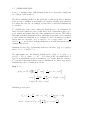
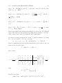
Step 1: β0
p(β0 |y, β1 , σe2 )
Y 1 1/2
1
2
exp − 2 (yi − β0 − xi β1 )
∝
σe2
2σe
i
"
#
N 2
1 X
∝ exp − 2 β0 + 2
(yi − xi β1 )β0 + const
2σe
σe i
= exp aβ02 + bβ0 + const
Matching powers gives:
σβ20 = −
1
σ2
= e
2a
N
1 X
(yi − xi β0 ),
N i
!
1 X
σe2
(yi − xi β1 ),
N i
N
and µβ0 = bσβ20 =
and so p(β0 |y, β1 , σe2 ) ∼ N
8
CHAPTER 1.
Step 2: β1
p(β1 |y, β0 , σe2 )
Y 1 1/2
1
2
exp − 2 (yi − β0 − xi β1 )
∝
2
σ
2σe
e
i
"
#
1 X 2 2
1 X
∝ exp − 2
xβ +
(yi − β0 )xi β1 + const
2σe i i 1 σe2 i
Matching powers gives:
P
(yi − β0 )xi
P 2
=
and µβ1 =
,
xi
i
P i

P
yi xi − β0 xi
2
σ
P 2 i
, Pe 2 
and so p(β1 |y, β0 , σe2 ) ∼ N  i
xi
xi
σβ21
σe2
1
=− = P 2
2a
xi
bσβ21
i
i
i
Step 3: 1/σe2
ε−1
1/2
1
ε Y 1
1
1
2
p
|y, β0 , β1 ∝
exp − 2
exp − 2 (yi − β0 − xi β1 )
σe2
σe2
σe i
σe2
2σe
"
!#
N2 +ε−1
1
1X
1
exp − 2 ε +
(yi − β0 − xi β1 )2
∝
σe2
σe
2 i
!
1X 2
1
N
|y, β0 , β1 ∼ Γ ε + , ε +
e
and so p
σe2
2
2 i i
So in this example we see that we can perform one iteration of our Gibbs
sampling algorithm by taking three random draws, two from Normal distributions and one from a Gamma distribution. It is worth noting that
P the
first two conditional distributions contain summary statistics, such as
x2i ,
i
which are constant throughout the sampling and used at every iteration. To
simplify the code and speed up estimation it is therefore worth storing these
summary statistics rather than calculating them at each iteration. Later in
this chapter we will give code so that you can try running this model yourself.
1.6
Metropolis Hastings sampling
When the conditional posterior distributions do not have simple forms we
will consider a second MCMC method, called Metropolis Hastings sampling.
1.6. METROPOLIS HASTINGS SAMPLING
9
In general MCMC estimation methods generate new values from a proposal
distribution that determines how to choose a new parameter value given
the current parameter value. As the name suggests a proposal distribution
suggests a new value for the parameter of interest. This new value is then
either accepted as the new estimate for the next iteration or rejected and the
current value is used as the new estimate for the next iteration. The Gibbs
sampler has as its proposal distribution the conditional posterior distribution,
and is a special case of the Metropolis Hastings sampler where every proposed
value is accepted.
In general almost any distribution can be used as a proposal distribution. In
MLwiN, the Metropolis Hastings sampler uses Normal proposal distributions
centred at the current parameter value. This is known as a random-walk
proposal. This proposal distribution, for parameter θ at time step t say, has
the property that it is symmetric in θ(t − 1) and θ(t), that is:
p(θ(t) = a|θ(t − 1) = b) = p(θ(t) = b|θ(t − 1) = a)
and MCMC sampling with a symmetric proposal distribution is known as
pure Metropolis sampling. The proposals are accepted or rejected in such
a way that the chain values are indeed sampled from the joint posterior
distribution. As an example of how the method works the updating procedure
for the parameter β0 at time step t in the Normal variance components model
is as follows:
1. Draw β0∗ from the proposal distribution β0 (t) ∼ N(β0 (t − 1), σp2 ) where
σp2 is the proposal distribution variance.
2. Define rt = p(β0∗ , β1 (t − 1), σe2 (t − 1)|y)/p(β0 (t − 1), β1 (t − 1), σe2 (t −
1)|y) as the posterior ratio and let at = min(1, rt ) be the acceptance
probability.
3. Accept the proposal β0 (t) = β0∗ with probability at , otherwise let
β0 (t) = β0 (t − 1)
So from this algorithm you can see that the method either accepts the new
value or rejects the new value and the chain stays where it is. The difficulty
with Metropolis Hastings sampling is finding a ‘good’ proposal distribution
that induces a chain with low autocorrelation. The problem is that, since
the output of an MCMC algorithm is a realisation of a Markov chain, we are
making (auto)correlated (rather than independent) draws from the posterior
distribution. This autocorrelation tends to be positive, which can mean that
the chain must be run for many thousands of iterations to produce accurate
posterior summaries. When using the Normal proposals as above, reducing
the autocorrelation to decrease the required number of iterations equates to
finding a ‘good’ value for σp2 , the proposal distribution variance. We will see
later in the examples the methods MLwiN uses to find a good value for σp2 .
10
CHAPTER 1.
As the Gibbs sampler is a special case of the Metropolis Hastings sampler,
it is possible to combine the two algorithms so that some parameters are
updated by Gibbs sampling and other parameters by Metropolis Hastings
sampling as will be shown later. It is also possible to update parameters
in groups by using a multivariate proposal distribution and this will also be
demonstrated in the later chapters.
1.7
Running macros to perform Gibbs sampling and Metropolis Hastings sampling
on the simple linear regression model
MLwiN is descended from the DOS based multilevel modelling package MLn
which itself was built on the general statistics package Nanostat written by
Professor Michael Healy. The legacy of both MLn and Nanostat lives on in
MLwiN within its macro language. Most functions that are performed via
selections on the menus and windows in MLwiN will have a corresponding
command in the macro language. These commands can be input directly
into MLwiN via the Command interface window available from the Data
Manipulation menu. The list of commands and their parameters are covered in the Command manual (Rasbash et al., 2000) and in the interactive
help available from the Help menu.
The user can also create files of commands for example to set up a model
or run a simulation as we will talk about in Chapter 8. These files can be
created and executed via the macros options available from the File menu.
Here we will look at a file that will run our linear regression model on the
tutorial dataset described in the next chapter.
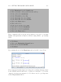
We will firstly have to load up the tutorial dataset:
• Select Open Sample Worksheet from the File menu.
• Select tutorial.ws from the list of possible worksheets.
When the worksheet is loaded its name (plus filepath) will appear at the top
of the screen and the Names window will appear giving the variable names
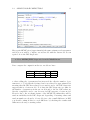
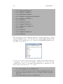
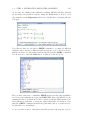
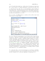
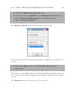
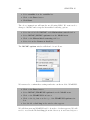
in the worksheet. We now need to load up the macro file:
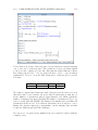
• Select Open Macro from the File menu.
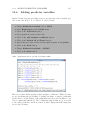
• Select gibbslr.txt from the list of possible macros.
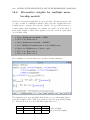
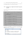
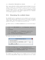
When the macro has been loaded a macro window showing the first twenty
or so lines of the macro will appear on the screen:
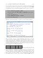
1.7. MACROS TO PERFORM GIBBS AND MH SAMPLING
11
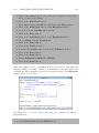
You will notice that the macro contains a lot of lines in green beginning with
the word note and this command is special in that it is simply a comment
used to explain the macro code and does nothing when executed. The macro
sets up starting values and then loops around the 3 steps of the Gibbs sampling algorithm as detailed earlier for the number of stored iterations (b17)
plus the length of the burn-in (b16).
To run the macro we simply press the Execute button on the macro window.
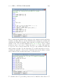
The mouse pointer will turn into an egg timer while the macro runs and then
back to a pointer when the macro has finished. The chains of values for the
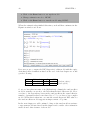
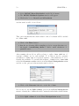
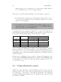
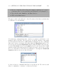
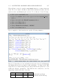
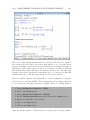
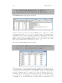
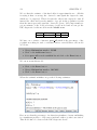
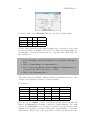
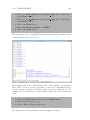
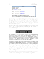
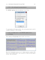
three parameters have been stored in columns c14–c16 and we can look at
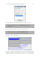
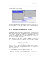
some summary statistics via the Averages and Correlations window
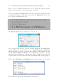
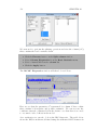
• Select Averages and Correlations from the Basic Statistics
menu
If we now scroll down the list of columns we can select the three output
columns that contain the chains, these have been named beta0, beta1 and
sigma2e. Note to select more than one column in this and any other window
press the ‘Ctrl’ key when you click on the selection with the mouse. When
the three are selected the window should look as follows:
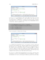
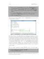
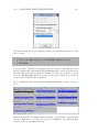
Now to display the estimates:
12
CHAPTER 1.
• Click the Calculate button
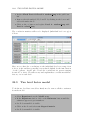
and the output window will appear with the following estimates:
These estimates are almost identical to those produced by the MLwiN MCMC
engine. Any slight differences will be due to the stochastic nature of MCMC
algorithms and will reduce as the number of updates is increased.
1.8
Dynamic traces for MCMC
One feature that is offered in MLwiN and some other MCMC based packages
such as WinBUGS (Spiegelhalter et al., 2000a) is the ability to view estimate
traces that update as the estimation proceeds. We can perform a crude
version of this with our macro code that we have written to fit this model. If
you scan through the code you will notice that we define a box b18 to have
value 50 and describe this in the comments as the refresh rate. Near the
bottom of the code we have the following switch statement:
calc b60 = b1 mod b18
switch b60
case 0:
pause 1
leave
ends
The box b1 stores the current iteration and all this switch statement is really
saying is if the iteration is a multiple of 50 (b18) perform the pause 1
command. The pause 1 command simply releases control of MLwiN from
the macro for a split second so that all the windows can be updated. This
will be how we set up dynamic traces and we will use this command again
in the simulation chapter later.
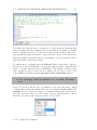
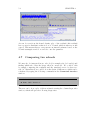
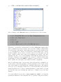
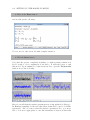
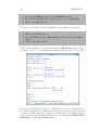
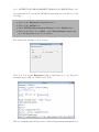
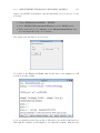
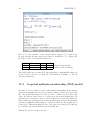
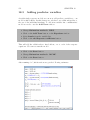
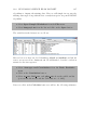
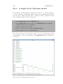
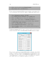
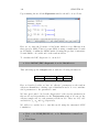
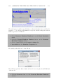
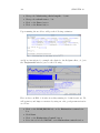
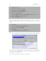
We now have to set up the graphs for the traces. The Customised graph
window is covered in reasonable detail in Chapter 5 of the User’s Guide to
MLwiN and so we will abbreviate our commands here for brevity. Firstly:
1.8. DYNAMIC TRACES FOR MCMC
13
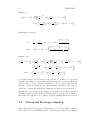
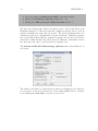
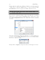
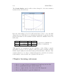
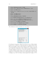
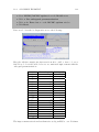
• Select the Customised Graph(s) option from the Graph menu
This will bring up the blank Customised graph window:
We will now select three graphs (one for each variable).
• Select beta0 from the y list
• Select itno from the x list
• Select line from the plot type list
This will set up the first graph (although not show it yet). We now need to
add the other two graphs:
• Select ds#2 (click in Y box next to 2) on the left of the screen.
• If this is done correctly the settings for all the plot what? tabs will
reset.
• Select beta1 from the y list.
• Select itno from the x list.
• Select line from the plot type list.
• Now select the position tab.
• Click in the second box in the first column of the grid.
• If this is done correctly the initial X will vanish and appear in this
new position.
Finally for parameter 3:
• Select ds#3 (click in Y box next to 3) on the left of the screen.
• Select sigma2e from the y list.
14
CHAPTER 1.
• Select itno from the x list.
• Select line from the plot type list.
• Now select the position tab.
• Click in the third box in the first column of the grid.
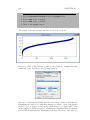
• Click on Apply and the 3 graphs will be drawn.
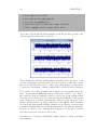
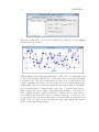
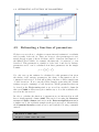
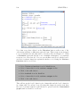
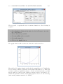
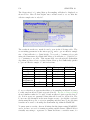
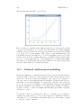
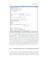
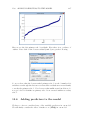
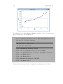
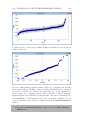
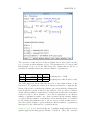
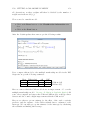
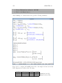
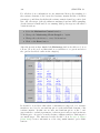
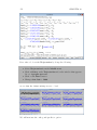
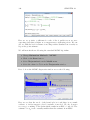
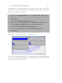
As we have already run the Gibbs sampler we should get three graphs of the
5000 iterations for these runs as follows:
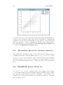
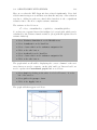
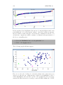
These chains show that the Gibbs sampler is mixing well as the whole of the
posterior distribution is being visited in a short period of time. We can tell
this by the fact that there are no white large white patches on the traces.
Convergence and mixing of Markov chains will be discussed in later chapters.
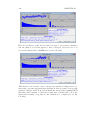
If we wish to now have dynamic traces instead we can simply restart the
macro by pressing the Execute button on the macro window. Note that as
the iterations increase estimation will now slow down as the graphs redraw
all points every refresh! Note also that after the chains finish you will get the
same estimates as you had for the first run. This is because the macro has a
Seed command at the top. This command sets the MLwiN random number
seed used and although the MCMC estimation is stochastic, given the same
parameter starting values and random numbers it is obviously deterministic.
It is also possible to have dynamic histogram plots for the three variables
but this is left as an exercise for the reader.
We will now look at the second MCMC estimation method: Metropolis Hastings sampling.
1.9. MACRO TO RUN A HYBRID SAMPLING METHOD
1.9
15
Macro to run a hybrid Metropolis and
Gibbs sampling method for a linear regression example
Our linear regression model has three unknown parameters and we have
in the above macro updated all three using Gibbs sampling from the full
conditional posterior distributions. We will now look at how we can replace
the updating steps for the two fixed parameters, β0 and β1 with Metropolis
steps.
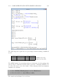
We first need to load up the Metropolis macro file:
• Select Open Macro from the File Menu.
• Select mhlr.txt from the list of possible macros.
We will here discuss the step to update β0 as the step for β1 is similar. At
each iteration, t, we firstly need to generate a new proposed value for β0 , β0∗ ,
and this is done in the macro by the following command:
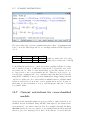
calc b30 = b6+b32*b21
Here b30 stores the new value (β0∗ ), b6 is the current value (β0 (t − 1)),
b32 is the proposal distribution standard deviation and b21 is a random
Normal(0,1) draw.
Next we need to evaluate the posterior ratio. It is generally easier to work
with log-posteriors than posteriors so in reality we work with the log-posterior
difference, which at step t is:
rt = p(β0∗ , β1 (t − 1), σe2 (t − 1)|y)/p(β0 (t − 1), β1 (t − 1), σe2 (t − 1)|y)
= exp(log(p(β0∗ , β1 (t − 1), σe2 (t − 1)|y))
− log(p(β0 (t − 1), β1 (t − 1), σe2 (t − 1)|y)))
= exp(dt )
We then have
dt = −
1
·
2σe2 (t − 1)
X
(yi − β0∗ − xi β1 (t − 1))2
i
!
−
X
i
(yi − β0 (t − 1) − xi β1 (t − 1))2
16
CHAPTER 1.
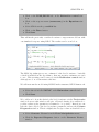
which with expansion and cancellation of terms can be written as
!
X
X
1
· 2
dt = − 2
yi − β1 (t − 1)
xi
2σe (t − 1)
i
i
· β0 (t − 1) − β0∗ + N ((β0∗ )2 − β02 (t − 1))
!
We evaluate this in the macro with the command
calc b34 = -1*(2*(b7-b31)*(b15-b6*b12) + b13*(b31*b31 b7*b7))/(2*b8)
Then to decide whether to accept or not, we need to compare a random
uniform with the minimum of (1, exp(dt )). Note that if dt > 0 then exp(dt ) >
1 and so we always accept such proposals and in the macro we then only
evaluate exp(dt ) if dt > 0. This is important because as dt becomes larger,
exp(dt ) → ∞ and so if we try and evaluate it we will get an error. The
accept/reject decision is performed via a SWITch command as follows in
the macro:
calc b35 = (b34 > 0)
switch b35
case 1 :
note definitely accept as higher likelihood
calc b6 = b30
calc b40 = b40+1
leave
case 0 :
note only sometimes accept and add 1 to b40 if accept
pick b1 c30 b36
calc b6 = b6 + (b30-b6)*(b36 < expo(b34))
calc b40 = b40 + 1*(b36 < expo(b34))
leave
ends
Here b40 is storing the number of accepted proposals. As the macro language does not have an if statement the calc b6 = b6 + (b30-b6)*(b36 <
expo(b34)) statement is equivalent to an if that keeps b6 (β0 ) at its current
value if the proposal is rejected and sets it to the proposed value (b30) if it
is accepted.
The step for β1 has been modified in a similar manner. Here the log posterior
1.9. MACRO TO RUN A HYBRID SAMPLING METHOD
17
ratio at iteration t after expansion and cancellation of terms becomes
!
X
X
1
· 2
xi yi − β0 (t)
dt = − 2
xi
2σe (t − 1)
i
i
X !
x2i
· β1 (t − 1) − β1∗ ) + ((β1∗ )2 − β12 (t − 1) ·
i
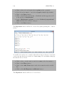
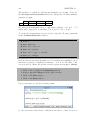
To run this second macro we simply press the Execute button on the macro
window. Again after some time the pointer will have changed back from the
egg timer and the model will have run. As with the Gibbs sampling macro
earlier we can now look at the estimates that are stored in c14–c16 via the
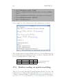
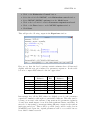
Averages and Correlations window. This time we get the following:
The difference in the estimates between the two macros is small and is due
to the stochastic nature of the MCMC methods. The number of accepted
proposals for both β0 and β1 is stored in boxes b40 and b41 respectively
and so to work out the acceptance rates we can use the command interface
window:
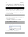
• Select Command Interface from the Data Manipulation menu.
• Type the following commands:
Calc b40=b40/5500
Calc b41=b41/5500
These commands will give the following acceptance rates:
->calc b40=b40/5500
0.75655
->calc b41=b41/5500
0.74291
So we can see that both parameters are being accepted about 75% of the
time. The acceptance rate is inversely related to the proposal distribution
variance and one of the difficulties in using Metropolis Hastings algorithms
is choosing a suitable value for the proposal variance. There are situations
to avoid at both ends of the proposal distribution scale. Firstly choosing
18
CHAPTER 1.
too large a proposal variance will mean that proposals are rarely accepted
and this will induce a highly autocorrelated chain. Secondly choosing too
small a proposal variance will mean that although we have a high acceptance
rate the moves proposed are small and so it takes many iterations to explore
the whole parameter space again inducing a highly autocorrelated chain. In
the example here, due to the centering of the predictor we have very little
correlation between our parameters and so the high (75%) acceptance rate
is OK. Generally however we will aim for lower acceptance rates.
To investigate this further the interested reader might try altering the proposal distribution standard deviations (the lines calc b32 = 0.01 and calc
b33 = 0.01 in the macro) and seeing the effect on the acceptance rate. It is
also interesting to look at the effect of using MH sampling via the parameter
traces described earlier.
1.10
MCMC estimation of multilevel models
in MLwiN
The linear regression model we have considered in the above example can
be fitted easily using least squares in any standard statistics package. The
MLwiN macro language that we have used to fit the above model is a compiled language and is therefore computationally fairly slow. In fact the speed
difference will become evident when we fit the same model with the MLwiN
MCMC engine in the next chapter. If users wish, to improve their understanding of MCMC, they can write their own macro code for fitting more
complex models in MCMC and the algorithms for many basic multilevel
models are given in Browne (1998). Their results could then be compared
with those obtained using the MCMC engine.
The MCMC engine can be used to fit many multilevel models and many
extensions. As was described earlier, MCMC algorithms involve splitting
the unknown parameters into blocks and updating each block in a separate
step. This means that extensions to the standard multilevel models generally
involve simply adding extra steps to the algorithm. These extra steps will
be described when these models are introduced.
In the standard normal models that are the focus of the next few chapters we
use Gibbs sampling for all steps although the software allows the option to
change to univariate Metropolis sampling for the fixed effects and residuals.
The parameters are blocked in a two level model into the fixed effects, the
level 2 random effects (residuals), the level 2 variance matrix and the level
1 variance. We then update the fixed effects as a block using a multivariate
normal draw from the full conditional, the level 2 random effects are updated
in blocks, 1 for each level 2 unit again by multivariate normal draws. The
level 2 variance matrix is updated by drawing from its inverse-Wishart full
1.10. MCMC ESTIMATION OF MULTILEVEL MODELS IN MLWIN 19
conditional and the level 1 variance from its inverse Gamma full conditional.
For models with extra levels we have additional steps for the extra random
effects and variance matrix.
Chapter learning outcomes
? Some theory behind the MCMC methods
? How to calculate full conditional distributions
? How to write MLwiN macros to run the MCMC methods
? How MLwiN performs MCMC estimation.
20
CHAPTER 1.
Chapter 2
Single Level Normal Response
Modelling
In this chapter we will consider fitting simple linear regression models and
normal general linear models. This will have three main aims: to start the
new user off with models they are familiar with before extending our modelling to multiple levels; to show how such models can be fitted in MLwiN,
and finally to show how these models can be fit in a Bayesian framework and
to introduce a model comparison diagnostic DIC (Spiegelhalter et al., 2002)
that we will also be using in the models in later chapters.
We will consider here an examination dataset stored in the worksheet tutorial.ws. This dataset will be used in many of the chapters in this manual
and is also the main example dataset in the MLwiN user’s guide (Rasbash
et al., 2008). To view the variables in the dataset you need to load up the
worksheet as follows:
• Select Open Sample Worksheet from the File menu.
• Select tutorial.ws.
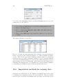
This will open the following Names window:
Our response of interest is named normexam and is a (normalised) total
exam score at age 16 for each of the 4059 students in the dataset. Our
21
22
CHAPTER 2.
main predictor of interest is named standlrt and is the (standardised) marks
achieved in the London reading test (LRT) taken by each student at age
11. We are interested in the predictive strength of this variable and we can
measure this by looking at how much of the variability in the exam score is
explained by a simple linear regression on LRT. Note that this is the model
we fitted using macros in the last chapter.
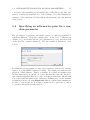
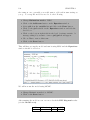
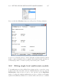
We will set up the linear regression via MLwiN’s Equations window that can
be accessed as follows:
• Select Equations from the Model menu.
The Equations window will then appear:
How to set up models in MLwiN is explained in detail in the User’s Guide
to MLwiN and so we will simply reiterate the procedure here but generally
less detail is given in this manual.
We now have to tell the program the structure of our model and which
columns hold the data for our response and predictor variables. We will
firstly define our response (y) variable to do this:
• Click on y (either of the y symbols shown will do).
• In the y list, select normexam.
We will next set up the structure of the model. We will be extending the
model to 2 levels later, so for now we will specify two levels although the
model itself will be 1 level. The model is set up as follows:
• In the N levels list, select 2-ij.
• In the level 2(j): list, select school.
• In the level 1(i): list, select student.
• Click on the done button.
In the Equations window the red y has changed to a black yij to indicate
that the response and the first and second level indicators have been defined.
We now need to set up the predictors for the linear regression model:
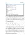
23
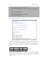
• Click on the red x0 .
• In the drop-down list, select cons.
Note that cons is a column containing the value 1 for every student and
will hence be used for the intercept term. The fixed parameter tick box
is checked by default and so we have added to our model a fixed intercept
term. We also need to set up residuals so that the two sides of the equation
balance. To do this:
• Check the box labelled i(student).
• Click on the Done button.
Note that we specify residuals at the student level only as we are fitting a
single-level model. We have now set up our intercept and residuals terms
but to produce the linear regression model we also need to include the slope
(standlrt) term. To do this we need to add a term to our model as follows:
• Click the Add Term button on the tool bar.
• Select standlrt from the variable list.
• Click on the Done button.
Note that this adds a fixed effect only for the standlrt variable. Until we
deal with complex variation in a later chapter we will ALWAYS only have
one set of residuals at level 1, i.e. only one variable with the level 1 tick box
checked.
We have now added all terms for the linear regression model and if we look
at the Equations window and:
• Click the + button on the tool bar to expand the model definition
we get:
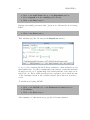
24
CHAPTER 2.
If we substitute the third line of the model into the second line and remember
that cons = 1 for all students we get yij = β0 + β1 standlrtij + eij , the
standard linear regression formula. To fit this model we now simply:
• Click Start.
This will run the model using the default iterative generalised least squares
(IGLS) method. You will see that the model only takes one iteration to converge and this is because for a 1 level model the IGLS algorithm is equivalent
to ordinary least squares and the estimates produced should be identical to
the answer given by any standard statistics package regression routine. To
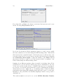
get the numerical estimates:
• Click twice on the Estimates button.
This will produce the following screen:
Here we see that there is a positive relationship between exam score and
LRT score (slope coefficient of 0.595). Our response and LRT scores have
been normalised i.e. they have mean 0 and variance 1, and so the LRT scores
explain (1 − 0.648) × 100 = 35.2% of the variability in the response variable.
As this manual is generally about the MCMC estimation methods in MLwiN
we will now fit this model using MCMC. Note that it is always necessary
in MLwiN to run the IGLS or RIGLS estimation methods prior to running
MCMC as these methods set up the model and starting values for the MCMC
methods.
To run MCMC:
• Click on the Estimation Control button
• Select the tab labelled MCMC
The window should then look as follows:
25
As described in the previous chapter MLwiN uses a mixture of Gibbs sampling steps when the full conditionals have simple forms, and Metropolis
Hastings steps when this is not the case. Here the estimation control window
shows the default settings for burn-in length, run length, thinning and refresh
rate. All other MCMC settings are available from the Advanced MCMC
Methodology Options window available from the MCMC submenu of the
Model menu.
In this release of MLwiN the user does not have to choose between Gibbs
sampling and Metropolis Hastings sampling directly. The software chooses
the default (and most appropriate) technique for the given model, which
in the case of Normal response models is Gibbs sampling for all parameters.
The user can however modify the estimation methods used on the Advanced
MCMC Methodology Options window that will be discussed later.
The four boxes under the heading Burn in and iteration control have the
following functions:
Burn-in Length. This is the number of initial iterations that will not be
used to describe the final parameter distributions; that is they are discarded
and used only to initialise the Markov chain. The default of 500 can be
modified.
Monitoring Chain Length. The monitoring period is the number of iterations, after the burn-in period, for which the chain is to be run. The default
of 5000 can be modified. Distributional summaries for the parameters can
be produced either at the end of the monitoring run or at any intermediate
time.
Thinning. This is the frequency with which successive values in the Markov
chain are stored. This works in a more intuitive way in this release, for
example running a chain for a monitoring chain length of 50,000 and setting
thinning to 10 will result in 5,000 values being stored. The default value of 1,
which can be changed, means that every iteration is stored. The main reason
to use thinning is if the monitoring run is very long and there is limited
memory available. In this situation this parameter can be set to a higher
integer, k, so that only every k-th iteration will be stored. Note, however,
26
CHAPTER 2.
that the parameter mean and standard deviation use all the iteration values,
no matter what thinning factor is used. All other summary statistics and
plots are based on the thinned chain only.
Refresh This specifies how frequently the parameter estimates are refreshed
on the screen during the monitoring run within the Equations and Trajectories windows. The default of 50 can be changed.
For our simple linear regression model we will simply use the default settings.
With regards to prior distributions we will also use the default priors as
described in the last chapter. In this release for clarity the prior distributions
are included in the Equations window. They can be viewed by:
• Clicking on the + button on the toolbar.
This will then give the following display (note the estimates are still the IGLS
estimates as we have not yet started the MCMC method.)
2.1
Running the Gibbs Sampler
We will now run the simple linear regression model using MCMC. Before
we start we will also open the Trajectories window so that we can see the
dynamic chains of parameter estimates as the method proceeds (note that
although viewing the chains is useful the extra graphical overhead means
that the method will run slower).
• Select Trajectories from the Model menu.
It is best to reposition the two windows so that both the equations and chains
are visible then we start estimation by:
2.1. RUNNING THE GIBBS SAMPLER
27
• Clicking the Start button.
The words Burning In. . . will appear for the duration of the burn in period. After this the iteration counter at the bottom of the screen will move
every 50 iterations and both the Equations and Trajectories windows will
show the current parameter estimates (based on the chain means) and standard deviations. After the chain has run for 5,000 iterations the trajectories
window should look similar to the following:
These graphs show the estimates for each of the three parameters in our
model and the deviance statistic for each of the last 500 iterations. The
numbers given in both the Equations window and the Trajectories window
are the mean estimates for each of the parameters (including the deviance)
based on the run of 5,000 iterations (with the standard deviation of these
5,000 estimates given in brackets). It should be noted that in this example
we have almost identical estimates as the least squares estimates which given
we have used ‘diffuse’ priors is reassuring.
Healthy Gibbs sampling traces should look like any of these iteration traces;
when considered as a time series these traces should resemble ‘white noise’.
At the bottom of the screen you will see two default settings. The first allows
you to choose how many values to view and here we are showing the values
for the previous 500 iterations only; this can be changed. The second drop
down menu allows you to switch from showing the actual chain values to
viewing the running mean of each parameter over time. It is possible to get
more detailed information about each parameter and to assess whether we
have run our chains for long enough. For now we will assume we have run
for long enough and consider MCMC diagnostics in the next chapter.
28
CHAPTER 2.
2.2
Deviance statistic and the DIC diagnostic
The deviance statistic (McCullagh and Nelder, 1989) can be thought of as a
measure of how well our model fits the data. Generally the deviance is the
difference in −2×log(likelihood) values for the fitted model and a saturated
model. In the normal model case we have:
N
1 X
N
2
(yi − ŷi )2
log(likelihood) = − log(2πσ̂e ) − 2
2
2σ̂e i=1
where N is the number of lowest level units (students) in the dataset, σ̂e2 is
an estimate of the level 1 variance and ŷi is the predicted value for student i,
in the case of the linear regression model ŷi = β̂0 + Xi β̂1 . For the saturated
model we have yi = ŷi ∀i and so the second term in the log-likelihood equals
zero. In the diagnostic that follows we are interested in differences in the
deviance and so we will assume the deviance of the saturated model is zero
as this term will cancel out.
Spiegelhalter et al. (2002) use the deviance with MCMC sampling to derive
a diagnostic known as the Deviance Information Criterion (DIC), which is a
generalization of the Akaike’s Information Criterion (AIC - See MLwiN help
system for more details). The DIC diagnostic is simple to calculate from an
MCMC run as it simply involves calculating the value of the deviance at each
iteration, and the deviance at the expected value of the unknown parameters
(D(θ̄)). Then we can calculate the ‘effective’ number of parameters (pD ) by
subtracting D(θ̄) from the average deviance from the 5000 iterations (D̄).
The DIC diagnostic can then be used to compare models as it consists of the
sum of two terms that measure the ‘fit’ and the ‘complexity’ of a particular
model,
DIC = D̄ + pD = D(θ̄) + 2pD = 2D̄ − D(θ̄).
It should be noted that the DIC diagnostic has not had universal approval and
the interested reader should read the discussion of the paper. Note that in
normal response models we have the additional parameter σ̂e2 . In calculating
D(θ̄)we use the arithmetic mean of σ̂e2 , (E(σe2 )) as this generalizes easily to
multivariate normal problems.
To calculate the DIC diagnostic for our model:
• Select MCMC/DIC diagnostic from the Model menu.
This will bring up the Output window with the following information:
Dbar D(thetabar) pD
DIC
9763.54
9760.51 3.02 9766.56
2.3. ADDING MORE PREDICTORS
29
Note that the value 9760.51 for D(θ̄) is (almost) identical to the −2×loglikelihood value given for the IGLS method for the same model. For 1 level
models this will always be true but when we consider multilevel models this
will no longer be true. Also in this case the effective number of parameters
is (approximately) the actual number of parameters in this model. When we
consider fitting multilevel models this will again no longer be the case.
2.3
Adding more predictors
In this dataset we have two more predictors we will investigate, gender and
school gender. Both of these variables are categorical and we can use the
Add term button to create dummy variable fixed effects, which are then
added to our model. To set up these new parameters we MUST change
estimation mode back to IGLS/RIGLS before altering the model.
• Click on the IGLS/RIGLS tab on the Estimation control window.
We now wish to set up a model that includes an effect of gender (girl) and
two effects for the school types (boysch and girlsch) with the base class for
our model being a boy in a mixed school. To set this up in the main effects
and interactions window we need to do the following:
• Click on the Add Term button on the Equations window.
• Select girl from the variable pull-down list.
The Specify term window should look as follows:
Now if we click on the Done button a term named girl will be added to the
model. We need now to additionally add school gender effects:
30
CHAPTER 2.
• Click on the Add Term button on the Equations window.
• Select schgend from the variable pull down list.
• Click on the Done button.
Having successfully performed this operation we will run the model using
IGLS.
• Click on the Start button.
This will then give the following in the Equations window:
So we see (by comparing the fixed effects estimates to their standard errors)
that in mixed schools, girls do significantly better than boys and that students
in single sex schools do significantly better than students of the same sex in
mixed schools. These additional effects have explained only a small amount
of the remaining variation, the residual variance has reduced from 0.648 to
0.634.
To fit this model using MCMC:
• Click on the MCMC tab on the Estimation Control window.
• Click Done.
• Click on the Start button.
After running for 5000 iterations we get the following estimates:
2.3. ADDING MORE PREDICTORS
31
Here again MCMC gives (approximately) the same estimates as least squares
and if we now wish to compare our new model with the last model we can
again look at the DIC diagnostic:
• Select MCMC/DIC diagnostic from the Model menu.
If we compare the output from the two models we have:
Dbar D(thetabar) pD
DIC
9763.54
9760.51 3.02 9766.56
9678.19
9672.21 5.99 9684.18
so that adding the 3 parameters has increased the effective number of parameters to 6 (5.99) but the deviance has been reduced by approximately 88
meaning that the DIC has reduced by around 82 and so the DIC diagnostic
suggests this is a better model. Note that the DIC diagnostic accounts for
the number of parameters in the two models and so the two DIC values are
directly comparable and so any decrease in DIC suggests a better model.
However due to the stochastic nature of the MCMC algorithm there will be
random variability in the DIC diagnostic depending on starting values and
random number seeds and so if a model gives only a small difference in DIC
you should confirm if this is a real difference by checking the results with
different seeds and/or starting values.
32
CHAPTER 2.
2.4
Fitting school effects as fixed parameters
We have in the last model seen that whether a school is single sex or mixed
has an effect on its pupils’ exam scores. We can now take this one step
further (as motivation for the multilevel models that follow) by considering
fitting a fixed effect for each school in our model. To do this we will first
have to set up the school variable as categorical:
• Select Names from the Data Manipulation menu.
• Note that the school variable is highlighted.
• Click on the Toggle Categorical button on the Names window.
• Click on the Categories button.
• Click on the OK button on the window that appears.
This will set up school names coded school 1 to school 65 for schools 1 to
65 which will be OK for our purposes, however generally we could have input
all the categories for example school names here.
We will now use the Add Term button to set up the school effects. We will
for now replace the school gender effects as they will be confounded with the
school effects. Note again that as we are about to modify the model structure
we will need to:
• Change estimation mode to IGLS/RIGLS via the Estimation Control window.
Next we set up the fixed effects as follows:
• Click Estimates in the Equations window once.
• Click on the β4 (girlsch) term.
• Click on the Delete Term button and respond Yes to removing all
schgend terms.
• Select the Add Term button from the Equations window.
• Select school from the variable list and click on the Done button.
This will now have removed the schgend terms from the model and set up
64 dummy variables for the school fixed effects using school 1 as a base
category. You will notice that all the school fixed effects have now been
added to the model in the Equations window:
2.4. FITTING SCHOOL EFFECTS AS FIXED PARAMETERS
33
• Click the Start button.
This will run the model using least squares (in 1 iteration) and give estimates for the 64 school effects. Note that these effects can be thought of as
differences in average achievement for the 64 schools when compared to the
base school. To fit this model in MCMC we need to:
• Select MCMC from the Estimation menu.
• Click on the Start button.
This model has 67 fixed effects and so even with the block updating Gibbs
sampling algorithm it will take a few minutes to run for 5000 iterations. After
running we see that the estimate for the base school (β0 ) is 0.341 (0.090) so
that this school is significantly better than average (for a boy with average
standlrt mark) and all other school effect estimates (β3 ,. . . ,β66 ) are relative
to this school.
If we were to check the DIC diagnostic for this model we have:
Dbar D(thetabar)
pD
DIC
9183.46
9115.36 68.10 9251.56
The DIC value has reduced from 9684 in our last model to 9252, a reduction of
432 points showing that the school in which the student studies has a strong
effect on their exam mark. Note that the effective number of parameters,
68.10, is still approximately correct for this model.
2
The variance estimate σe0
has now been reduced to 0.563 and so we have now
explained 43.7% of the variation in our original response with the addition
of 67 fixed effects.
In this example we have introduced fixed school effects and shown that we
actually do not need to fit a random effects model to account for school differences. We will however in the next chapter introduce multilevel modelling
by fitting school effects as random terms and explain why and when this may
be a better approach.
Chapter learning outcomes
34
CHAPTER 2.
? How to set up models in MLwiN using the Equations window.
? How to set up 1 level models in MLwiN.
? How to run the MCMC Gibbs sampling method.
? How to access and interpret the DIC diagnostic.
? How to fit a fixed effects model.
Chapter 3
Variance Components Models
We ended the last chapter with an example of how to fit school effects as
fixed terms in a linear model. In this chapter we will introduce fitting these
same school effects as random terms. Whether you choose to fit terms as
fixed or random is one of the main difficulties faced by researchers new to
multilevel modelling. In some scenarios the answer is obvious but in other
situations which model you fit will very much depend on what your main
research questions are and the context in which the data are collected.
Here we consider how to add a categorical explanatory variable to our model.
Certain categorical variables, for example gender and school gender in the
tutorial example, will ALWAYS be fitted as fixed effects. This is because
these variables have a limited number of categories and all categories are
present in the dataset. The motivation behind fitting a categorical variable,
for example school, as a set of random effects is that the categories of this
variable that we observe are, in fact, a sample of the possible categories.
Then, just like our observations at level 1, we can think of our categories
as being a sample from a population of categories and make a distributional
assumption about these categories.
The main reason for fitting a categorical variable as a random term rather
than as fixed effects is if our primary interest is in the variability across
the various categories rather than inferences about any single category. For
example we may want to calculate how much of the variability in our outcome
variable is due to the schools attended and how much is residual variation due
to pupil differences. Also as we may only have a small sample of level 1 units
for each category, the random effects produced will be more conservative than
the category effects produced by a fixed effect model. This is because we use
the fact that categories, for examples schools, are similar to each other, in
that case we may borrow strength from the other schools and when we wish
to estimate them, we “shrink” the school effects towards the average school
effect.
35
36
CHAPTER 3.
In multilevel modelling when we treat a categorical variable as a set of random
effects we describe the set of categories as a level in the model. This is because
our observations (level 1 in the model) are nested within these categories, for
example pupils are nested within schools. The level terminology can be
extended for example to 3 levels if we want to extend our model to contain
both effects for schools, and for the local education authorities (LEAs) to
which the schools belong. Here we have a nesting of pupils within schools and
schools within LEAs and hence a 3 level structure. Note that we will see in
later chapters that structures are not always nested, leading to cross-classified
structures. Here we will use the alternative terminology of classification
rather than level.
Levels are not the same as random effects as there may be several sets of
random effects at a level; such models, called random slopes regression models, are described in a later chapter. Having more than one set of random
effects in a model can be thought of as the random equivalent of having an
interaction between a categorical variable and another explanatory variable
in the model as we will see in the later chapter.
For now, to distinguish between levels and random effects, we will have school
as the level and the school intercepts as the random effects.
3.1
A 2 level variance components model for
the Tutorial dataset
We will now return our attention to the tutorial dataset. At the end of the
last chapter we had fitted the school fixed effects model. This time we will
fit a school random effects model. To do this we will have to remove all the
fixed effects that are currently in the model, This may be done by reloading
the worksheet tutorial.ws or:
• In the Equations window click on the Clear button.
This will reset our model and we will have to set up our model from scratch.
Now we need to set up the linear regression model that contains the intercept
and the standlrt explanatory variable, which was fitted first in the last
chapter. (If you are unsure how to do this follow the instructions in the last
chapter.)
We now have to add random school level intercepts to the model. Note that
to do this you should have the estimation method set to IGLS. The variable
cons is associated with the intercepts and so you need to do the following:
3.1. A 2 LEVEL VARIANCE COMPONENTS MODEL
37
• Click on cons
and the following X variable screen will appear:
We now need to:
• Click on the i(student) box
• Click on the j(school) box
• Click on the Done button
to allow for level 1 variation and random intercepts for each school. Note that
you may already have the i(student) box ticked from the regression in which
case you need to ensure it is still ticked. The model we have now set up is a
member of the variance components family. A model is called a variance
components model if there is only one set of random effects (intercepts) for
each level in the model. This is because the model splits the total variation
into components of variation for each level in the model. The particular
variance components model with an intercept and slope term in the fixed
part is often called a random intercepts model. This is because graphically
(as shown in the User’s Guide to MLwiN), each school can be represented
by a (parallel) regression line with a fixed slope and a random intercept.
We will now run the model firstly using IGLS to obtain starting values, and
then using MCMC with the default settings:
• Click on the Start button.
• Select MCMC from the Estimation menu.
• Click on the Start button.
Again if you have the Equations and Trajectories windows open you will
see the estimates and traces change as the estimation proceeds. Upon completion of the 5,000 iterations the Trajectories window should look as follows:
38
CHAPTER 3.
Here we see that, unlike the linear regression example in the last chapter,
these traces do not all look healthy and the trace for β0 looks quite autocorrelated i.e. each value of the trace is highly correlated with the preceding
value. We can get more detailed diagnostic information about a parameter,
for example the slope coefficient β1 , by clicking the left mouse button on
the parameter trace for β1 . The program will then ask ‘Calculate MCMC
diagnostics?’ to which you should click on Yes. The message “Calculating
MCMC diagnostics . . . May take a while.” will then appear and after a
short wait you will see a diagnostics screen similar to the following:
The upper left-hand cell simply reproduces the whole trace for the parameter.
The upper right-hand cell gives a kernel density (which is like a smoothed
histogram) estimate of the posterior distribution; when an informative prior
distribution is used the density for this distribution is also displayed in black
(see examples in later chapters). We can see in this example that the density
looks to have approximately a Normal distribution. The second row of boxes
plots the autocorrelation (ACF) and partial autocorrelation (PACF) functions. The PACF has a small spike at lag 1 indicating that Gibbs sampling
3.1. A 2 LEVEL VARIANCE COMPONENTS MODEL
39
here behaves like a first order autoregressive time series with a small autocorrelation of about 0.1. The ACF is consistent with this suggesting that the
chain is adequately close to independently identically distributed (IID) data
(autocorrelation 0).
The third row consists of some accuracy diagnostics. The left-hand box
plots the estimated Monte Carlo standard error (MCSE) of the posterior
estimate of the mean against the number of iterations. The MCSE
is an
√
indication of the accuracy of the mean estimate (MCSE = SD/ n, where
SD is the standard deviation from the chain of values, and n is the number
of iterations). This graph allows the user to calculate how long to run the
chain to achieve a mean estimate with a particular desired MCSE. The righthand box contains two contrasting accuracy diagnostics. The Raftery-Lewis
diagnostic (Raftery & Lewis, 1992) is a diagnostic based on a particular
quantile of the distribution. The diagnostic Nhat is used to estimate the
length of Markov chain required to estimate a particular quantile to a given
accuracy. In MLwiN the diagnostic is calculated for the two quantiles (the
defaults are the 2.5% and 97.5% quantiles) that will form a central interval
estimate. For this parameter the estimated chain length (Nhat) is 3,804 for
both quantiles (note this is unusual and generally the quantiles will have
different Nhat values) so having run the chain for 5,000 iterations we have
satisfied this diagnostic. The Brooks-Draper diagnostic is a diagnostic based
on the mean of the distribution. It is used to estimate the length of Markov
chain required to produce a mean estimate to k significant figures with a given
accuracy. Here we can see that to quote our estimate as 0.56 (2 significant
figures) with the desired accuracy requires the chain to be run only for 30
iterations so this diagnostic is also satisfied for this parameter.
The interpretation of the numbers q = (0.025,0.975), r = 0.005 and s = 0.95
in the Raftery-Lewis diagnostic is as follows: With these choices the actual
Monte Carlo coverage of the nominal 100(0.975 − 0.025)% = 95% interval
estimate for the given parameter should differ by no more than 100(2×r)% =
1 percentage point with Monte Carlo probability 100×s = 95%. The values
of q, r and s can be changed.
The bottom box contains some numerical summaries of the data. As well as
the mean (with its MCSE in parenthesis), this box also contains the mode
and median estimates. To estimate both 90% and 95% intervals this box also
contains the appropriate quantiles of the distribution. For example a 95%
central interval (Bayesian credible interval) runs from 0.539 to 0.588.
Also in the bottom row of the box details of the run length of the Markov
chain are given. We also include an estimate of the effective (independent)
sample size (see Kass et al., 1998). Here the number of stored iterations is
divided by a measure of the correlation of the chain called the autocorrelation
time κ where
∞
X
κ=1+2
ρ(k)
k=1
40
CHAPTER 3.
To approximate this value, we evaluate the sum up to k = 5 and then every
subsequent value of k until ρ(k) < 0.1. So in this example we have an almost
independent chain and our actual sample of 5,000 iterations is equivalent to
an independent sample of 4,413 iterations.
Note that many of the settings on the diagnostics screen can be changed from
their default values. For more information on changing the diagnostics screen
settings see the on-line Help system. To see a somewhat different picture you
can shut down this window and click, for example, on the plot for the level
2 variance in the Trajectories window (shown below).
Here we can see in the kernel density plot that the posterior distribution
is not symmetric which is to be expected for a variance parameter. The
Raftery-Lewis diagnostics suggest that we have run for long enough although
to quote the mean estimate as 0.097 with 95% confidence the Brooks-Draper
diagnostic suggests we run for 11,365 iterations. We see in the summary
statistics that the 90% and 95% central credible interval that we can calculate
from the quantiles will reflect the skewed nature of the posterior distribution.
Also we see that the mode is less than the mean due to the long tail to the
right of the distribution.
Finally, we can compare the results from Gibbs to the results from the IGLS
method for this model in the following table:
Parameter
β0
β1
2
σu0
2
σe0
Gibbs
Mean
0.005
0.563
0.097
0.566
Posterior
SD
0.042
0.012
0.021
0.013
IGLS
Mean SD
0.002 0.040
0.563 0.012
0.092 0.018
0.566 0.013
The only real difference is the slightly higher value for the Gibbs estimate of
3.2. DIC AND MULTILEVEL MODELS
41
the level 2 variance. The Gibbs estimate for the mode of 0.092 (see above)
is identical to the IGLS estimate (to 3 decimal places) since the maximum
likelihood estimate approximates (in effect) the posterior mode (with a diffuse prior) rather than the mean. In some situations, the choice of diffuse
prior (for the variance parameter) will be important, in particular when the
underlying variance is close to zero and poorly estimated (i.e. with a large
standard error). This may be particularly noticeable in random coefficient
models and is a topic of current research (Browne, 1998). We will talk about
the choice of prior in more detail in a later chapter.
3.2
DIC and multilevel models
We can now work out the DIC diagnostic for this model via the Model
menu:
• Select MCMC/DIC diagnostic from the Model menu.
Dbar D(thetabar)
pD
DIC
9209.15
9146.16 59.98 9269.13
Here we will notice a difference between random effects models and fixed
effects models. If we were to assume fixed school effects then our model
would have 65 school intercepts plus the level 1 variance plus the fixed slope
effect resulting in 67 parameters. Here however the school effects are related
through the fact that they have a common variance structure and so we do not
have independent 67 parameters. In fact, in this model the DIC diagnostic
estimates the number of independent parameters to be approximately 60.
3.3
Comparison between fixed and random
school effects
In the last chapter we fitted a fixed effects model that also included a gender
effect. We can now add this gender term into our above model. To do this
we need to do the following:
• Change estimation mode to IGLS.
• Click on the Add term button in the Equations window.
• Select girl from the variable list and click on the Done button.
42
CHAPTER 3.
• Click on the Start button to set up the model.
• Change estimation mode to MCMC.
• Click on the Start button to run the model using MCMC.
When the estimation has finished this time you should have estimates in the
Equations window as follows:
If we were now to compare the DIC diagnostic for this model with the equivalent fixed effect formulation fitted at the end of the last chapter we would
get the following:
Dbar D(thetabar)
pD
DIC
9184.93
9124.37 60.56 9245.49 (random effects)
9183.46
9115.36 68.10 9251.56 (fixed effects)
So we see here that in terms of fit (D(thetabar) column) the random effect
model is actually a worse fit to the data than the fixed effects model. However due to the dependency between the random effects the actual effective
number of parameters has been reduced by ≈ 7.5 so we have a less complex
model. When this is taken into account the actual diagnostic DIC value for
the random effects model suggests an improvement of 6 points.
In the next chapter we will continue looking at the random effects variance
components model introduced in this chapter and consider other estimation
methods and other features of the model
3.3. FIXED VS. RANDOM SCHOOL EFFECTS
Chapter learning outcomes
? What is meant by fixed effects, random effects and levels.
? How to set up a variance components model
? How to get more MCMC diagnostic information in MLwiN
? How to compare the fit of random and fixed effect models.
43
44
CHAPTER 3.
Chapter 4
Other Features of Variance
Components Models
In this chapter we will return to the variance components model we considered in the last chapter. We will firstly show how to fit this model using the
other MCMC methods available in MLwiN. We will then look at some other
features of the variance components model for example residuals, school ranks
and the intra-school correlation. The final model we considered in Chapter 3
had gender effects that we will now remove. To remove a term from a model
we do the following:
• Select IGLS from the Estimation menu.
• Click on the girl variable in the Equations window.
• From the X variable screen that appears click on Delete Term.
• Run this model with the IGLS method by clicking on the Start
button.
The Equations window should now look as follows:
45
46
CHAPTER 4.
4.1
Metropolis Hastings (MH) sampling for
the variance components model
Although for Normal response models the default MCMC method is Gibbs
sampling for all parameters, we can still use other methods via the Advanced
MCMC Methodology Options window. Metropolis Hastings sampling is
particularly useful for multilevel generalised linear models as will be seen in
the later chapters of this manual. We shall firstly see how it can be used
on a normal response variance components model. To use MH sampling, go
back to the Estimation control window and click on MCMC. Then select
MCMC/MCMC methods from the Model menu, which will bring up
the following window:
This window contains the options to change the estimation methods used
for various groups of parameters as well as other advanced options including
a selection of Metropolis Hastings settings. As the window shows you can
change the MCMC method used for both the fixed effect parameters and the
residuals (the variance parameters are always updated by the Gibbs sampling
method). To use Metropolis Hastings sampling:
• Select the method Univariate MH for the fixed effects.
• Select the method Univariate MH for the random effects (residuals).
• Select the Done button.
We now look at how to use the settings.
4.2. METROPOLIS-HASTINGS SETTINGS
4.2
47
Metropolis-Hastings settings
The performance of the Metropolis Hastings method depends very much on
the proposal distribution used. A proposal distribution that accepts too
many or too few proposals will produce highly autocorrelated chains. In
MLwiN, the Metropolis Hastings sampler has some additional settings to
help choose ‘good’ proposal distributions for the parameters. There are two
strategies that can be used in MLwiN to produce good proposal distributions.
Firstly it was shown in Gelman, Roberts & Gilks (1995) that for a simple
Normal posterior distribution, a univariate Normal proposal distribution with
a variance 5.8 times the true variance of the parameter is the best proposal
distribution. Hence in MLwiN the user has the option to input a scale factor
for proposal variances. This number will then be multiplied by the estimated
parameter variance (from IGLS/RIGLS) to give the proposal distribution
variance. Although this works for single level Normal models, studies of
multilevel models (Browne, 1998) have shown that the factor 5.8 is not always
the best and is often too high.
The second approach, the adaptive method, which is used by default in the
development release of MLwiN is to find proposal distributions that give a
particular desired acceptance rate. Experience suggests that rates of between
30% and 70% provide a useful compromise between a proposal variance that
is too large and a variance that is too small. If the proposal variance is
too large, the chain stays where it is for long periods before making a large
jump, whereas if it is too small the chain makes lots of little moves but takes
a long time to explore the whole sample space. MLwiN finds the desired
proposal distribution by running an adapting period before the burn in. In
this adapting period the proposal distribution is modified to improve the
acceptance rate.
The settings screen contains two boxes labelled desired acceptance rate
(default 50%) and desired tolerance (default 10%). If the adaptive method
is selected then when you click on the Start button, MLwiN will make an
exploratory run of up to 5,000 iterations while displaying the message ‘Running Adaptive procedure and Burning in’. During this period the proposal
variance is modified every hundred iterations depending on the acceptance
rate in the current batch of hundred iterations to ensure that the acceptance
rates for all parameters are as close to 50% as possible, and in the range
50%−10%=40% to 50%+10%=60%. Once this is achieved the adapting period ends and the burn in begins as with Gibbs sampling.
We will now look at running the variance components model with the adaptive method.
48
CHAPTER 4.
4.3
Running the variance components with
Metropolis Hastings
After setting up the variance components model as before and running the
IGLS method to get starting values, the Metropolis Hastings sampler was
run with the default settings. After 5,000 iterations clicking on the graph for
β1 in the Trajectories window you should now see diagnostics for β1 similar
to the following:
We can now see that both accuracy diagnostics give Nhat values that are
considerably higher than for Gibbs sampling so that for this model MH would
take longer than Gibbs sampling to give the same accuracy. We also see that
the first order autocorrelation is about 0.65, which is substantially higher
than for Gibbs and results in an effective sample size of only 973. This also
implies a longer chain length is needed. If we run the MH sampler without
the adaptive method, we obtain a slightly higher Nhat value of about 16,400
for the Raftery-Lewis diagnostic for the 2.5% quantile.
The following table compares parameter estimates from IGLS, Gibbs and
MH with both the scale factor and adaptive methods.
Parameter
β0
β1
2
σu0
2
σe0
IGLS Gibbs MH Scale Factor MH Adaptive
= 5.8 with defaults
0.002 0.005
0.013
-0.005
0.563 0.563
0.563
0.563
0.092 0.097
0.097
0.097
0.566 0.566
0.566
0.566
MH and Gibbs sampling show good agreement, and apart from the level two
variance parameter there is good agreement with RIGLS too. The estimates
of the intercept β0 show some variability but this is because this parameter
has larger Nhat values and so the chains have not been run for long enough
4.4. MH CYCLES PER GIBBS ITERATION
49
and in all cases this parameter is effectively zero. It is often useful with
MCMC estimation to try both Gibbs and MH to confirm your estimates.
We will now describe some additional MH features available in MLwiN.
4.4
MH cycles per Gibbs iteration
The parameter MH cycles per Gibbs iteration governs how many times
the steps for the parameters being estimated by MH are run for each iteration.
This is useful as the MH method tends to give higher autocorrelations than
the Gibbs sampling method. For example if the parameter is set to 3 in
the above example, the Raftery Lewis Nhat for β1 reduces to 5,973 and the
autocorrelation of its chain is reduced to 0.4 (ESS increased to 2,406). Note
that this reduction in autocorrelation has to be balanced by the increase in
time to run the model and in this case the 5000 iterations takes just under
double the time.
4.5
Block updating MH sampling
As described earlier, the Gibbs sampling estimation method in MLwiN updates the parameters in blocks; all fixed effects are updated together as are
all the level 2 residuals for one level 2 unit (for a variance components model
there is only 1 residual per level 2 unit). In contrast the MH estimation
method uses univariate updates for each parameter separately. In this development release, a block updating MH method is also available. This method
updates the parameters in the same blocks used by the Gibbs sampling
method.
Parameters are updated in blocks using multivariate Normal proposals that
take account of the correlation between the parameters in the block. As
several parameters are updated together acceptance rates for each block will
be lower than the acceptance rates achieved by updating each parameter
individually, although updating the block should be faster than updating each
parameter individually. The block updating sampler constructs a proposal
based on the covariance matrix of the parameters in the block and a tuning
constant. See Browne & Draper (2000) for more details.
In the variance components example, there is only one set of level 2 residuals but two fixed effects. Consequently changing the estimation method to
Multivariate MH, i.e. block updating, will have no effect for the residuals
but will have an effect for the fixed effects. After running IGLS, bring up
the Advanced MCMC Methodology Options window and change the
settings as follows:
50
CHAPTER 4.
• Select the method Multivariate MH for the fixed effects.
• Change the Desired acceptance rate (%) to 40.
• Change the MH cycles per Gibbs iteration back to 1.
We have here changed the desired acceptance rate to 40% in the Metropolis
Hastings settings box. This is because the optimal acceptance rate for a block
update is smaller the larger the block size. The block updating method is
currently regarded as ‘experimental’ because ideally the optimal acceptance
rate for the fixed effects and the optimal acceptance rate for the level 2 residuals will be different when the block sizes are different. Currently however
the user may only enter a global desired acceptance rate.
The Advanced MCMC Methodology Options window should then look
as follows:
The method was run for 5,000 iterations after an adapting period and trajectory traces of the last 50 iterations of the chains (which can be obtained
by modifying the view last box) can be seen below:
4.6. RESIDUALS IN MCMC
51
On close inspection it can be seen that the two chains for the fixed effects,
β0 and β1 , are being updated as a block, as the jumps caused by accepted
proposals occur simultaneously. Note that sometimes (for example β0 in the
last iteration) the accepted new value is very similar to the current value.
We will now return to Gibbs sampling and consider other features of the
variance components model. First we must reset all of the MCMC settings:
• Select IGLS and run the model (press the Start button).
• Change estimation mode to MCMC
• Select MCMC/MCMC Methods from the Model menu.
• Click on the Reset button.
• Click on the Done button.
4.6
Residuals in MCMC
Although a multilevel model contains many parameters, by default when
running MCMC sampling, the full MCMC chains are only stored for the
fixed effects and variance parameters. For the residuals, only means and
standard errors are stored from their chains. It is then these values that
are used when the residuals options, as demonstrated in the User’s Guide to
MLwiN Chapter 3, are used whilst running MCMC. If however an accurate
interval estimate or other summary statistics are required for a residual then
there is also the option of storing all the residuals at a given level.
To store residuals will generally require a large amount of memory as there
are generally a large number of residuals per level. We will consider storing
only the level 2 residuals here, although even then we will have 65 residuals,
one per school. To store residuals:
52
CHAPTER 4.
• Select MCMC/Store Residuals from the Model menu.
• The MCMC Residuals Options window will appear.
• Click in the box to Store Level 2 Residuals.
and the window will look as follows:
This option means that the chain values for the 65 residuals will be stacked
in column c301.
• Click on the Done button.
• Run the model using Gibbs sampling as before except this time set
the length of monitoring chain to 5001 to make calculation of
quantiles easier.
After running the model we will now have to split column c301 into 65
separate columns, one for each residual. To do this we need to generate
an indicator column that is a repeated sequence of the numbers 1 to 65 to
identify the residuals. To generate this sequence of numbers in column c302
select the Generate vector window from the Data Manipulation menu
and choose the options as shown in the window below:
• Click on the Generate button to create the column.
We now need to use the Split column option from the Data Manipulation
menu to identify the columns that will contain the individual residual chains:
• Select Split column from the Data Manipulation menu.
4.6. RESIDUALS IN MCMC
53
• For input columns, select c301 as the data column and
• Select c302 as the code column.
• Select c303-c367 as the output columns (use the Shift key or the Ctrl
Key along with the left mouse button to select multiple columns).
• Click on the Add to action list button.
The above set of instructions will then produce the following screen:
• Click on Execute to run the command
The columns c303-c367 will now contain the chains of the school level residuals.
We can name the columns c303-c367 if we wish by using the Names window and then display the MCMC diagnostics via the Column diagnostics
window that can be found under the Basic Statistics menu as follows:
Choose the column containing the residual for school 1 (c303) that has here
been named ‘school1’ via the Names window and click on Apply to see the
diagnostics as follows:
54
CHAPTER 4.
As can be seen from the kernel density plot of the residual, this residual
has a posterior distribution that is close to Normal, which is what we would
expect. This means that we can generate an interval estimate based on the
Normal assumption and do not need to use the quantiles.
4.7
Comparing two schools
We may also be interested in two schools (for example schools 1 and 2) and
finding which school has the larger effect in our model. We could do this
by simply comparing the residuals and the standard errors for these two
schools. Alternatively we could look at the chain of differences, which can be
calculated by typing the following commands in the Command interface
window:
Calc c368=c303-c304
Name c368 'Diff1-2'
Then we can look at a plot of this new function using the column diagnostics
window, which will give the following diagnostics:
4.8. CALCULATING RANKS OF SCHOOLS
55
Here we can see that the value 0 is inside both the 90% and 95% intervals
and so the two school residuals are not significantly different, although on
average school 2 is performing better than school 1.
We can again use the command interface window to see how often each school
performs better in these chains with the following commands:
Calc c369 = 'diff1-2' > 0
Aver c369
These two commands give the average 0.166 so that school 1 performs better
than school 2 in 16.6% of the iterations. This can be compared with the
1-sided P-value of 0.161 when testing whether this parameter is significantly
different from zero (assuming Normality).
4.8
Calculating ranks of schools
We may also be interested in the ranks of the schools rather than their actual
residuals and MCMC allows us to calculate point and interval estimates for
each school’s rank (see Goldstein & Speigelhalter, 1996).
Here we need to run several commands to split and sort the residuals and
then rank the schools and so we have included the required commands in the
macro rank.txt.
To open this macro:
• Select Open Macro from the File menu.
56
CHAPTER 4.
• Select rank.txt from the list of files.
• Click on the Open button.
The macro will then appear as follows:
This macro will give chains for the ranks of each school in columns c203c267. Run this macro now by clicking on the Execute button. Note that this
macro will take a bit of time to run. It would be useful from this to calculate
a ‘caterpillar’ style plot for the ranks and the following macro rank2.txt
(which can be opened and run after the rank.txt macro) calculates the
median, 2.5% and 97.5% quantiles for each school.
4.8. CALCULATING RANKS OF SCHOOLS
57
Note that this macro will reuse the columns in which the 65 residual chains
were stored earlier. We can then graph the schools by using the Customised
graph window; we first set up the x and y variables as follows:
Next we set up the limits on the error bars tab as follows:
58
CHAPTER 4.
Then the graph will look as follows (with titles added) once the Apply
button has been pressed:
This graph shows the ranks (plus intervals) for all 65 schools, noting that rank
65 here is the highest achieving school and rank 1 the lowest (after adjusting
for intake score). We can see that there is often great overlap between the
relative rankings of the schools and in many cases great uncertainty in the
actual ranks. We can convert the graph into the more common ‘caterpillar’
plot by replacing the ‘y’ variable with ‘mean’, the ‘x’ variable with ‘rankno’.
This sorts the schools according to rank rather than numeric order. The error
bars columns should be replaced with the columns ‘ulmean’ and ‘llmean’.
Note that the mean has been used to calculate ranks (to avoid ties) so the
points plotted are now mean ranks and not median ranks as in the previous
graph. Note also that we have rescaled the axes and changed the symbol
used for the points in this graph.
4.9. ESTIMATING A FUNCTION OF PARAMETERS
4.9
59
Estimating a function of parameters
We have now seen how to calculate accurate interval estimates for residuals
and for ranks of the schools. There are however other parameters not estimated directly as part of the model that could be of interest. In Chapter 2 of
the MLwiN User’s Guide, for example, the intra-school correlation, ρs , was
described. This parameter is a function of the level 1 and level 2 variance
parameters and so can be calculated from these parameters via the simple
formula:
ρs = σu2 /(σu2 + σe2 )
Not only can a point estimate be calculated for this parameter but given
the chains of the variance parameters, the chain of this function can be
constructed and viewed. You should at this point have a Gibbs sampler run
of 5001 iterations. If not, run the Gibbs sampler again using the default
settings except for running for 5,001 iterations. All the parameters that can
be viewed in the Trajectories window are stored in a stacked column (in
this case C1090 is always used) in a similar way to how the residuals were
stored in the last section.
In order to calculate the function of parameters we are interested in we will
have to firstly unstack column c1090. This can be done using the Generate
vector and Split column windows from the Data manipulation menu in
a similar way to the residuals example in the previous section. Alternatively
the Command interface window can be used and the following commands
entered:
code 4 1 5001 c300
split c1090 c300 c301-c304
60
CHAPTER 4.
Having split the variables into different columns we can then name the
columns either by using the Names window or again by using the Command Interface window by typing the NAME command as follows:
name c301 'beta0' c302 'beta1' c303 'lev2var' c304
'lev1var' c305 'ISC'
We now need to calculate the chain of values for the intra-school correlation
(ISC) and we do this by using the Calculate window, which can be found
in the Data Manipulation menu. The column ‘ISC’ should be calculated
as follows:
Then after calculating the chain for the intra-school correlation function we
now need to use the Column Diagnostics window from the Basic Statistics menu to display the chain:
Having clicked on Apply the diagnostics window should appear as follows:
4.9. ESTIMATING A FUNCTION OF PARAMETERS
61
This window shows that although we are not sampling the derived variable
ISC directly we can still monitor its Markov chain. This has the advantage
that we can now calculate an accurate interval estimate for this function.
Chapter learning outcomes
? How to change MCMC estimation method from Gibbs sampling to
MH sampling for some steps of the algorithm.
? What other MCMC settings there are and what they do.
? How to store residual chains
? How to calculate ranks of schools
? How to calculate estimates and chains for derived variables
62
CHAPTER 4.
Chapter 5
Prior Distributions, Starting
Values and Random Number
Seeds
In this chapter we consider some other features of the MCMC estimation
procedures in MLwiN. We will still consider the variance components model
with one predictor (standlrt) discussed in the last two chapters and will
look at how to modify the prior distributions, starting values and random
number seeds used for this model.
5.1
Prior distributions
In Chapter 1 we described the default prior distributions used in MLwiN. We
also mentioned that these defaults are different (for the variance parameters)
from the priors used in the first version of MLwiN (release 1.0). This is
because these new priors generally give less positive bias when the parameter
estimate based on the mean is used. The old default priors can still be
selected via the MCMC window available from the Model menu, as can
informative priors.
5.2
Uniform on variance scale priors
The default variance priors used in MLwiN (release 1.0) are now offered as
an alternative to the new default priors. The improper diffuse priors used
previously were as follows:
• For random parameters priors are placed on variances and covariance
63
64
CHAPTER 5.
matrices p(Ω) ∝ 1 (a constant prior over the positive definite matrices
Ω, or a uniform prior for σ 2 for a single variance)
These priors are functionally equivalent to the following proper priors:
• For single variance parameters, a Uniform prior U (0, c) where c is chosen so that (0, c) spans the range in which the likelihood for the parameter is non-negligible.
• To use these priors select Uniform on variance scale for the default diffuse priors for variance parameters on the MCMC priors
window available from the Model menu.
Comparing these priors (with the default Γ−1 (ε, ε) priors used thus far for
single variances) using the Gibbs sampler on the variance components model
we get the following results (using a monitoring run of 5,000):
Parameter
IGLS
Gibbs
(Γ (ε, ε) priors) (Uniform priors)
(0.040)
0.005 (0.042)
0.004 (0.042)
(0.012)
0.563 (0.012)
0.563 (0.013)
(0.018)
0.097 (0.021)
0.101 (0.022)
0.092
0.095
(0.013)
0.566 (0.013)
0.566 (0.013)
−1
2
σu0
2
σu0
β0
β1
(Mean)
(Mode)
2
σe0
0.002
0.563
0.092
0.566
So we see that the Uniform prior tends to give larger variance estimates
than the default priors when the number of level 2 units is small. Browne
(1998) and Browne & Draper (2006) show this in more detail via simulation
experiments and we will discuss running simulations in MLwiN in greater
detail in Chapter 8.
In this version of MLwiN it is also possible to change the parameters of the
Γ−1 priors via the MCMC/ priors window available from the Model menu.
The defaults are a = 0.001, b = 0.001 but another popular choice is to set
a = 1.0 and b = 0.001.
5.3
Using informative priors
MLwiN also allows the user to specify informative priors for any of the parameters in the model. This could be useful if the user already has some
prior knowledge on the values of the unknown parameters. We will firstly
consider specifying an informative prior for the fixed effect associated with
the intake score (LRT).
5.3. USING INFORMATIVE PRIORS
65
Again we will start with IGLS starting values so run the model using the
IGLS method. Then on the MCMC Priors window:
• Click on Gamma priors to return to the default variance priors.
• Click on the Informative Priors. . . button.
The following window will appear showing all the parameters in the model
(in this case the level 1 and level 2 covariance matrices contain just a single
variance term):
For the fixed parameters, informative priors are assumed to be Normal and
are chosen by specifying the mean and SD. The priors for a covariance matrix
are assumed to have an inverse Wishart distribution and the specification
is described in the next section. Note that for scalar variances, as in this
example, an informative inverse Gamma distribution will be used. We wish
to add a prior for the slope parameter, β1 . Let us assume, for illustration, that
from a previous study we have (after transformations) observed an estimated
coefficient of 1.0 for LRT intake score.
If you click on, for example, β1 , and then enter an informative prior with
a mean of 1 (remembering the posterior estimate from a ‘diffuse’ prior is
just over half this) and a prior SD of 0.01 (implying highly accurate prior
knowledge), and click on β1 again the window will appear as follows:
The asterisk that appears next to β1 indicates that a prior distribution has
been set for this parameter. (You can get back to the default by clearing the
values and clicking next to the asterisk.) Now:
• Click on the Done buttons to close down the two Priors windows.
• Click on the Start button to run the Gibbs sampler.
66
CHAPTER 5.
After 5000 iterations, if you click on the trajectories window for β1 , the
diagnostics plot will appear similar to that below:
Here we can see that the prior distribution (on the right) is included on the
kernel density plot in black and can thus be compared with the posterior
distribution, which is in blue. In this example the two distributions are
completely separated indicating a conflict between the prior and the data.
The estimate of the parameter is also very different from what we had before
(0.841 as opposed to 0.563) and the variance parameter estimates are also
rather different, which reduces the SD for β1 .
Now let us specify less accuracy for the prior by changing the value of SD
to 0.1 and running the model again. This time we obtain values for all
parameters that are very close to those of the default prior assumptions,
because the prior is now highly diffuse in relation to the data as is shown in
the kernel plot in the diagnostics below:
In this example there is a distinct difference in the prior value for β1 and
the estimate from this dataset. If however the prior and data are more in
5.4. INFORMATIVE PRIORS FOR RANDOM PARAMETERS
67
concordance then including an informative prior will reinforce the data estimate by reducing the standard error of the estimate. Note that changing the
structure of the current model will result in all informative prior information
being erased.
5.4
Specifying an informative prior for a random parameter
The procedure for specifying informative priors for random parameters is
somewhat different. Clear the existing prior on the slope coefficient (by
clicking on β1 and setting the two prior parameters to zero) and then click
on the level two variance matrix Ωu . The Priors window will then look as
follows:
For illustration let us assume we have a prior estimate of the level 2 variance
equal to 0.2 (the RIGLS estimate is 0.092). The sample size indicates the
precision of this estimate. Thus, for example, if you had an estimate from
another study based on 100 schools, you would enter the value 100. Let us do
this, remembering that there are 65 schools in the present study. MLwiN will
now convert this information into an Inverse Gamma prior for the variance
as illustrated in the following Equations window obtained after running the
model for 5,000 iterations. Note that you may need to press the + button
to get prior information in the window.
68
CHAPTER 5.
Here we see that the estimated value of the level two variance after 5,000
iterations is now 0.163 — fairly close to a weighted average of the estimate
obtained with a diffuse prior and the informative prior estimate (weighted
by the number of level two units the estimates are based on) — and the
other parameter estimates are hardly changed. Currently in MLwiN the
prior density is not shown for random parameters in the kernel plots. Before
going on to the next session we should remove the informative priors and
this is done by bringing up the Informative priors window and typing 0
for the sample size parameter.
5.5
Changing the random number seed and
the parameter starting values
The prior distributions described above actually change the model structure
when fitted using MCMC sampling. The parameters we describe in this
section do NOT change the form of the model but due to the stochastic
nature of the MCMC methods slightly different estimates may result from
modifying them. MCMC sampling involves making random draws from the
conditional posterior distributions of the various parameters in the multilevel
model. To start the MCMC sampler, starting values are required for each
parameter along with a starting value (a positive integer) for the random
number generator known as a seed. This means that given the starting values
of the parameters and the random number seed the sampling is deterministic
and so running the same model with the same starting values and seed on a
different machine will give the same answers.
5.5. CHANGING THE SEED AND THE STARTING VALUES
69
Most of the posterior distributions that can be run using MCMC in MLwiN
are known to be uni-modal. If this were not the case then it would be more
sensible to make several runs with different starting values to check that they
all reach similar final estimates. The starting values for the fixed effects and
variance parameters are taken from the values obtained by the last model
run. These values are stored on the worksheet in specific columns in the
MLwiN worksheet. The starting values for the residuals are then produced by
MLwiN calculating the maximum likelihood estimates for these parameters,
conditional on the values of the fixed effects and variance parameters (stored
in columns c1098 and c1096 respectively).
We will consider again our 2 level variance components model and run IGLS
on the model. If you then open the Data window as described below you
will see the following window.
• Select View or Edit Data from the Data Manipulation menu.
• Click on the View button.
• Select columns c1096 and c1098 (use the CTRL button to select
both).
• Click on OK.
We will now alter these estimates to values that are far less plausible. To
alter a value in the Data window, simply click on a cell in the window and
type the new value. The new values were chosen as follows:
Note that MLwiN uses the starting values of the other parameters to calculate
the starting values of the residuals, and so these new starting values cannot be
altered directly. It is however possible by using the Command interface
window to alter the values of the other parameters directly. To see the
progress of the chains from their starting values we will set the burn-in length
to 0 and the monitoring chain length to 500 in the Estimation Control
window as shown below.
70
CHAPTER 5.
If we then click on Start, the chains for the first 500 iterations can be seen
in the following Trajectories window:
By about 250 iterations all the parameters appear to settle out at roughly
the same estimates as seen when using the IGLS starting values. This means
that if we had set a burn-in length of 500 iterations we would not have even
seen this behaviour! If you now run for another 500 iterations (by changing
the monitoring chain length to 1000 and clicking on the More button)
the trajectories plots of the second 500 iterations will look similar to the
Gibbs chains using the IGLS starting values.
Running from different starting values is useful for checking that all the
parameters in your model have uni-modal posterior distributions. In some
of the new models in this release of MLwiN this may not be guaranteed.
If, however, it is already known that the posterior distributions should be
uni-modal it is best to utilise the ‘good’ starting values obtained by IGLS,
particularly when using MH sampling which may take longer to reach equilibrium (i.e. the point where it is actually sampling from the correct posterior
distribution).
The random number seed can be set on the MCMC/Random Number
5.6. IMPROVING THE SPEED OF MCMC ESTIMATION
71
Seed window available from the Model menu. Changing the random number seed is another technique that can be used to check that the MCMC
method is sampling correctly from the posterior distribution. Running from
the same starting values but with different random number seeds will give
different estimates but these estimates will hopefully be similar. Note that in
MLwiN the random seed for the MCMC options is different from the random
number seed used by the macro command language that can be set by the
SEED command. The MCMC seed can be set by the MCRS command.
To illustrate this behaviour the following table contains the point estimates
(for sets of 5000 iterations after burnins of 500) obtained for the variance
components model using the Gibbs sampler with random number seeds 1 to
4.
Parameter
β0
β1
2
σu0
2
σe0
Seed 1 Seed 2 Seed 3 Seed 4
0.005
0.003
0.002
0.004
0.563
0.563
0.563
0.564
0.097
0.097
0.097
0.097
0.566
0.566
0.566
0.566
This table clearly shows that there is little change in the parameter values
when we change the random number seed. This means we can have more
confidence in our estimates.
Note that making use of the options in this section is not generally required
to ensure good MCMC performance. We include them only for completeness.
5.6
Improving the speed of MCMC Estimation
One feature of MCMC estimation methods is that they are computationally
intensive, and generally take far longer to run than the likelihood-based IGLS
and RIGLS methods. This fact means that any possible speed up of execution
will be beneficial. There are two ways to speed up the execution of MCMC
estimation methods: first to minimise the number of iterations required to
give accurate estimates, and second to speed up the time for an individual
iteration.
One simple procedure to help minimise the number of iterations is to ensure
that all continuously distributed explanatory variables are centred at their
mean or something close to it. In the example analysed above the reading score predictor has already been standardised to have zero mean. This
will minimise correlations among parameters in the posterior, which should
increase MCMC accuracy.
We are continually trying to speed up the MCMC estimation procedures in
72
CHAPTER 5.
MLwiN and you should find that the speed of estimation is generally better
than some other general purpose Bayesian modelling software. With the
speed of computer chips also improving at an incredible rate the time taken
by MCMC methods is continually improving.
Although both the Equations and Trajectories windows are informative
to watch while the MCMC methods are running, they will both slow down
the estimation procedure. For example the following table shows some timings performed on a Pentium 666MHz PC, running the variance components
model for 5,000 iterations after a burn in of 500.
Screen Format
No windows
Equations window
Trajectories window
Both windows
20
25
34
38
Time
seconds
seconds
seconds
seconds
As can be seen, displaying the windows — particularly the Trajectories
window — slows the estimation down.
Chapter learning outcomes
? How to change the default variance prior distributions.
? How to specify informative prior distributions.
? How to modify both the parameter starting values and random number seed.
? How to speed up the methods.
Chapter 6
Random Slopes Regression
Models
In the past three chapters we have considered the variance components model
and looked at how we can apply different MCMC methods and priors to this
model. We have also looked at some of the features of the model such as
residuals and school ranks that can be calculated by the MCMC methods.
We saw that compared to the single level models from Chapter 2 the variance
components model—which has random intercepts—fits the data better. We
will now continue our exploration of the dataset by considering fitting both
random intercepts and slopes.
In Chapter 2 we saw that it is possible to account for school effects by fitting
an intercept and a fixed term for each school (with the constraint that the
fixed effect associated with school 1 is equal to 0) and that this results in
a model with 66 fixed effects. It is also possible to fit a fixed effect model
that accounts for both different school effects and different effects of intake
score (LRT) for each school. This involves fitting the ‘interaction’ of school
effect with LRT score and we will then have the two constraints that both
the fixed effect associated with school 1 and the intake effect for school 1 are
constrained to be zero. Note of course that this does not mean that school
1 has zero effects. School 1 is just the baseline school with regression line
explained by the common intercept and slope terms, and the other school
effects and LRT effects are then relative to this baseline school. To fit this
model in MLwiN we need to again use the Add Term button on the Equations window. We first set up the model with individual school effects as
described at the end of Chapter 2 but this time we will remove the effect of
gender. Note that if you are following on from the last chapter you should
also ensure the random number seed is set back to 1.
• In the Equations window click on β2 (girl) and click on the delete
term button.
73
74
CHAPTER 6.
• Click on the Add Term button.
• Select 1 in the order box.
• Select school as the first variable (the first box under variable).
• Select standlrt as the second variable.
The window should look as follows:
Now clicking on the Done button will add the 64 school by intake score
interaction terms.
This will now have set up the model with 130 fixed effects. If you have the
Equations window open you will notice that all the school × LRT terms
have been added to the model.
• Click the Start button.
This will run the model using ordinary least squares and give estimates for
the 130 fixed effects. Note that the school × LRT terms can be thought of
as slope differences when comparing these 64 schools to the base school. If
we were to re-parameterise the model by removing the global intercept and
slope and instead add the intercept and slope indicators for the base school
we will get exactly the same model but this time the parameters will be the
actual intercepts and slopes for each school. We are therefore essentially, in
this model, fitting separate regression lines to each school. To fit this model
in MCMC we need to:
• Select the MCMC tab on the Estimation Control window.
• Click on the Start button.
This model has 130 fixed effects and so will take a few minutes to run. If we
were to check the DIC diagnostic for this model we would obtain:
Dbar D(thetabar)
pD
DIC
9117.58
8987.00 130.59 9248.17
75
Here we see that the fit (D(thetabar)) is a lot better than the single level
models that were fitted in Chapter 2 but that we now have 131 parameters
and so the DIC value is only slightly better than the model with gender also
included (of course we could fit gender here as well which would improve the
fit further). The model we have just fitted is equivalent to fitting 65 separate regressions and so we are here considering each school as a completely
separate entity.
In Chapter 3 we considered fitting the school effects as random terms and we
can extend this idea by also considering the school×LRT effects as random.
Here again we are using the idea that the schools are randomly chosen. We
assume that schools are similar and so, as we have only taken a sample of
pupils from each school, we wish to borrow strength from the other schools
and shrink the LRT effects of each school towards the average LRT effect.
To fit the school effects as random we will first set up the variance components
model from the last chapter. To do this we will clear our model and set up
the variance components model from scratch (refer to Chapter 3 if you are
unsure of how to do this).
Next we need to add in the random effects for the standlrt (slope) variable:
• Click on standlrt in the Equations window.
• Click on the j(school) checkbox in the window that appears. This
allows random LRT effects for each school.
The model we have now set up is often called a random slopes regression
model as we can think of the LRT effects as slopes when we plot our predicted
response variable against the LRT predictor for each school. We will first run
the model using IGLS to obtain starting values before switching to MCMC:
• Click on the Start button.
• Click on the MCMC tab on the Estimation Control window.
• Click on the + button on the Equations window until prior distributions are shown.
After doing this the Equations window should look as follows:
76
CHAPTER 6.
We can see that for a model that contains a variance matrix rather than
a simple variance we use an inverse Wishart prior with as few degrees of
freedom as possible. The Wishart prior family is not as convenient as the
Gamma in that we have to include a prior guess for the variance matrix.
Here we have a slightly data determined prior as by default MLwiN will take
the current estimate of Ωu (from the IGLS run) as a prior parameter. We
will later compare this approach with some alternatives.
• Click the Start button to run the model.
The MCMC approach with default priors gives fairly similar estimates to the
maximum likelihood approach. The DIC diagnostic can be calculated for
this model and we find the following:
Dbar D(thetabar)
pD
DIC
9122.99
9031.32 91.67 9214.65
In treating both the intercepts and slopes as random parameters we have
reduced the effective number of parameters from 130.6 to 91.7. The fit of the
random effects model is 44 points worse but the DIC diagnostic (accounting
for the reduced number of parameters) suggests that this is a better model
as its value has been reduced from 9248 to 9215.
6.1. PREDICTION INTERVALS FOR A RANDOM SLOPES MODEL 77
6.1
Prediction intervals for a random slopes
regression model
In Chapter 4 of the User’s Guide to MLwiN details are given on how to use
the Predictions window to construct predicted school lines with confidence
intervals. Although we can construct a predicted line and intervals for the
fixed part of the model easily using MCMC to include the school effects in
the predictions we need to store the school level residuals as we require the
MCMC chains of the predicted values to produce quantiles and hence give
the prediction intervals.
To set things up we will firstly need to run a model with the residuals stored
as follows:
• Change estimation method to IGLS.
• Click on the Start button.
• Change estimation method to MCMC.
• On the Estimation Control window change the length of monitoring chain to 5001.
• Select MCMC/Store Residuals from the Model menu.
• Click in the box to Store Level 2 Residuals.
• Change Column number to c200.
• Click on the Done button.
• Click on the Start button.
This will run the random slopes model again, this time storing the residuals. We now need to create a point estimate (median) and interval estimate
(quantiles) for the predicted value for each individual. To do this we have
created a macro that generates the required quantities.
• Select Open Macro from the File menu.
• Select predint.txt from the list of files and click on the Open button.
The macro will now appear as shown below. This macro basically creates
the chain of predicted values for each individual and takes the quantiles and
median from this chain. Many of the commands are similar to those that we
used in Chapter 4 to look at the chains for the residuals and the intra-school
correlation.
78
CHAPTER 6.
We can now run the macro by clicking on the Execute button. Note that
this will take a couple of minutes. After the macro has finished to display
our predictions we can use the Customised graph window.
• Select Customised Graph from the Graph menu.
• Select pred as the y variable.
• Select standlrt as the x variable.
• Select school as the group variable.
• Select line as plot type.
• Click on the error bars tab.
• Select uplim as the y errors + variable.
• Select lowlim as the y errors − variable.
• Select lines as the y error type.
• Click on the Apply button to plot the graph.
The graph will appear as follows:
6.1. PREDICTION INTERVALS FOR A RANDOM SLOPES MODEL 79
Here we see all 65 school lines plus their intervals on one graph. Due to the
195 lines on the one graph it is difficult to pick out the individual schools.
We can however use a filter column to view just a few schools:
• Select Command Interface from the Data Manipulation menu.
• Type the following command to create the filter column:
calc c24='school'==30 | 'school'==44 | 'school'==53
| 'school'==59
• Select Customised Graphs from the Graphs menu.
• Select c24 as the filter variable.
• Note if the Customised Graphs window is already visible you may
need to close it and open it for c24 to appear in the pull down list.
• Click on the plot style tab.
• Change colour to 16-rotate.
• Click on the other tab.
• Click in the group code tickbox for key labels.
• Click on the Apply button.
The graphs for the four schools will then appear as follows:
80
CHAPTER 6.
So in this section we have shown that again when using MCMC methods,
because we have draws from the joint posterior distribution of all unknown
parameters, we can derive the distribution of any function of the parameters
such as a prediction. Before continuing this chapter and looking again at
prior distributions you should change the monitoring chain length back
to 5,000 on the Estimation Control window.
6.2
Alternative priors for variance matrices
The default prior distribution that we have used in this example involves
a slightly informative ‘data-determined’ prior for Ωu . Browne (1998) and
Browne & Draper (2000) perform some comparisons between some prior
distributions that can be used as a default for a variance matrix. We will
here, as a sensitivity analysis exercise, consider the effect of three alternative
priors.
6.3
WinBUGS priors (Prior 2)
Spiegelhalter et al. (2000b) consider in their ‘birats’ fitting a prior similar
to our default, namely an inverse-Wishart with the smallest possible sample
size and a prior guess that represents the magnitude of the variances. For
example here we may use the values 0.1 for both the variances. To fit this
prior we firstly need to:
6.4. UNIFORM PRIOR
81
• Run the model in IGLS
and then, as with when we changed the MCMC starting values, we can alter
the parameter values in c1096:
• Select View or Edit Data from the Data Manipulation menu.
• Click on the View button.
• Select column c1096 from the list.
This will bring up the data window and show the starting values for the variance parameters. We wish to change the first three values (level 2 variance).
Type 0.1,0, and 0.1 in the first three rows and the window should look as
follows:
Now we have the priors set up.
• Select MCMC from the Estimation menu.
• Click on the Start button.
The results for this prior are given in the column headed Gibbs (prior 2) at
the end of the chapter.
6.4
Uniform prior
Another alternative would be to fit a Uniform prior i.e. p(Ωu ) ∝ 1. To fit
this prior we need to once again fit the model using IGLS. Then we need to
change the default priors from gamma priors to Uniform on variance scale
priors on the MCMC priors window (available from the Model menu) as
shown below:
82
CHAPTER 6.
Note that this will change the prior for the level 1 variance as well. Fit this
model and the results will be as in the column Gibbs (uniform) in the table
at the end of the chapter.
6.5
Informative prior
Our final alternative is to assume (for illustration) that we had a priori
collected another dataset with 65 schools and here the estimated variance
matrix was identical to the IGLS estimate here. We then wish to use this as
a prior distribution so (after as always running IGLS first) we:
• Select the MCMC tab from the Estimation control window.
• Select MCMC/Priors from the Model menu.
• Select Gamma priors from the MCMC priors window (this sets
the prior for level 1 variance)
• Select Informative Priors from the MCMC priors window.
• Select Ωu from the top bar of the window.
• Input the estimates 0.09,0.018 and 0.015 in the estimate boxes (as
below).
• Input 65 in the sample size box.
• Click on Ωu again.
When this is done the Priors window should look as follows:
6.6. RESULTS
83
• Click the Start button.
The results can be seen in the fourth column labelled Gibbs (prior 4) in the
table below.
6.6
Results
The results for all 4 priors along with the IGLS estimates are given in the
following table (Standard Errors in brackets). We can see that the results for
all priors are similar which is reassuring. The second prior has an increased
slopes variance as the prior guess was quite a bit higher than the IGLS estimate. The Uniform prior (as in Browne & Draper, 2000) is conservative and
gives variance estimates that are biased high for all the variance parameters.
The informative prior gives almost identical posterior estimates to its prior
estimates, which is to be expected as we have given the prior equal weight to
the data. We also see that the standard errors of the level 2 variances have
reduced and so our estimates have greater precision. This is an advantage
of the Bayesian approach in that when we have ‘good’ prior information we
will get more precise estimates and hence smaller credible intervals.
Parameter
β0
β1
Ωu00
Ωu01
Ωu11
2
σe0
IGLS
-0.012
(0.040)
0.557
(0.020)
0.090
(0.018)
0.018
(0.007)
0.015
(0.004)
0.554
(0.012)
default
-0.006
(0.039)
0.558
(0.020)
0.096
(0.020)
0.019
(0.007)
0.015
(0.004)
0.554
(0.013)
prior 2
-0.007
(0.039)
0.556
(0.023)
0.096
(0.020)
0.018
(0.008)
0.023
(0.005)
0.553
(0.013)
Gibbs
uniform
-0.006
(0.042)
0.558
(0.022)
0.103
(0.022)
0.020
(0.008)
0.018
(0.005)
0.554
(0.013)
prior 4
-0.008
(0.042)
0.558
(0.020)
0.091
(0.012)
0.018
(0.004)
0.015
(0.002)
0.554
(0.013)
Chapter learning outcomes
? How to fit different LRT effects for each school in a fixed effects
model.
? How to fit a random slopes regression model.
84
CHAPTER 6.
? How to compare models via the DIC diagnostic.
? How to create prediction intervals for a model using MCMC.
? A greater understanding of prior distributions.
Chapter 7
Using the WinBUGS Interface
in MLwiN
We have so far looked at fitting Normal response models to continuous univariate data in MLwiN. We could consider fitting further models with additional fixed or random terms and these would simply be extensions to the
models fitted thus far. There are, however, other extensions that we could
consider; for example, heteroskedasticity of the response variable, which we
consider in Chapter 9 and alternative distributions for the random effects
that we will consider later in this chapter.
The MCMC features in MLwiN are fairly new and we currently fit only
models of particular types although we are constantly extending the number
of models that can be fitted. If, however, a user wishes to fit a model that
cannot be currently fitted, for example fitting an alternative distribution for
the school level random effects, there are three main options. Firstly wait
for a later version of MLwiN that will fit their model; secondly write their
own code to fit their model; or thirdly try an alternative software package,
for example WinBUGS.
WinBUGS (Spiegelhalter et al., 2000a, freely available from http://www.
mrc-bsu.cam.ac.uk/bugs) in its earlier guise of BUGS was one of the first
Bayesian software packages and is a more general purpose Bayesian estimation engine than the MCMC engine in MLwiN. It works on a different philosophy of fitting models that can be represented by directed acyclic graphs
(DAGs). BUGS has a compiled language which allows the user to specify
their model through statements of two types—logical and distributional—
which between them describe the structure of the DAG and hence the model.
Then BUGS compiles this user code and constructs an MCMC estimation
engine for the user’s model that can be run to give chains of estimates in a
similar way to the MLwiN engine.
In this chapter we will firstly consider once again the variance components
85
86
CHAPTER 7.
model and show how to fit this model in WinBUGS. We then go on to
consider a model that MLwiN cannot fit which has t-distributed residuals at
the school level. It should be noted at this point that most multilevel models
are large and so cannot be run using the educational version of WinBUGS
and so you will need to have the release version of WinBUGS.
7.1
Variance components models in WinBUGS
We will consider the tutorial dataset once again. Set up and run the variance
components model with one explanatory variable (standlrt) using the IGLS
method by
• Pressing the Start button
On IGLS convergence we get the following estimates:
In Chapter 3 we then considered fitting this model using MCMC in MLwiN
but here we will consider instead using WinBUGS. To get to the BUGS
options in MLwiN we need to do the following:
• Click on the Estimation Control button.
• Select the MCMC tab.
• Select MCMC/WinBUGS Options from the Model menu.
This will bring up the WinBUGS Options screen that looks as follows:
7.1. VARIANCE COMPONENTS MODELS IN WINBUGS
87
From this screen we can save the BUGS code for the currently set up model
or read in the output files that contain parameter traces from BUGS for use
in MLwiN (see later). For now we will save our current model in BUGS
format:
• Select the WinBUGS 1.4 button.
• Click on the large button at the top of the window.
This will bring up a file save window similar to those for inputting and
saving worksheets. For now we will save the file in the default directory
as tutorial.bug. This will create a file that contains the BUGS model
definition, initial values and data. For users of classic BUGS who are used
to having three separate files, in WinBUGS the file tutorial.bug contains
the information from these three files with comment lines dividing them. In
what follows we use WinBUGS version 1.4.3 and so it is possible that results
will change with other versions.
For background information on using WinBUGS it is strongly suggested that
the user reads some of the user manual and examples documentation that
comes with the package, in particular to become familiar with the WinBUGS
notation. For now to fit our model in WinBUGS, we must start the WinBUGS program and read in the file tutorial.bug (from the directory it was
saved in) as a text file. Note that you will have to change the Files of type
box to All files (*.*) to see the file tutorial.bug. Having read in the file a
window headed tutorial.bug will appear containing the information needed
by BUGS for this model.
As mentioned earlier the WinBUGS code is split into 3 sections and we will
consider these here in turn. Firstly a model definition is required and this
consists of a description of the structure of the current problem. The code
for our simple variance components problem is as follows:
# WINBUGS 1.4 code generated from MLwiN program
88
CHAPTER 7.
#----MODEL Definition---------------model
{
# Level 1 definition
for(i in 1:N) {
normexam[i] ∼ dnorm(mu[i],tau)
mu[i]<- beta[1] * cons[i]
+ beta[2] * standlrt[i]
+ u2[school[i]] * cons[i]
}
# Higher level definitions
for (j in 1:n2) {
u2[j] ∼ dnorm(0,tau.u2)
}
# Priors for fixed effects
for (k in 1:2) { beta[k] ∼ dflat() }
# Priors for random terms
tau ∼ dgamma(0.001000,0.001000)
sigma2 <- 1/tau
tau.u2 ∼ dgamma(0.001000,0.001000)
sigma2.u2 <- 1/tau.u2
}
WinBUGS is a more general modelling package and so there is no standard
order to the model description although when the code is generated from
MLwiN it will generally have a similar structure. We firstly define the relationship between the response (in this example normexam) and the fixed
and random predictor variables.
Note that the column names from MLwiN are used as the variable names
in WinBUGS. WinBUGS does have some differences in what it allows as a
variable name so if the WinBUGS code will not work it may be that some of
your variable names are illegal, for example a column name like 1995 will be
interpreted as a number in WinBUGS so it is worth renaming such columns
in MLwiN.
So we see here that our response is normally distributed and that we have
two fixed effects, beta[1] and beta[2] (always defined as beta by the code
generator) and one set of random effects, u2 (always defined as u# where
# is the level/classification indicator). Note that in WinBUGS the fixed
effects, beta, and all other vectors always start with index 1 and not 0 so that
there will probably not be direct correspondence between the MLwiN and
WinBUGS indexing. Next the code defines the random effects u2 as being
Normally distributed before finally giving the priors for the fixed effects and
the variances.
WinBUGS has two types of relationship: distributional relationships that
7.1. VARIANCE COMPONENTS MODELS IN WINBUGS
89
are described by the ∼ symbol and deterministic relationships that are described by the <- symbol which is also used in the S-plus package. Note that
the normal distribution definition in WinBUGS, dnorm, has two parameters
that are the mean and the precision (NOT the variance), hence the deterministic relationship used to calculate the variance. The prior distributions
are identical to those used in the MCMC options in MLwiN.
Before running a model in WinBUGS we first need to read in the particular
elements of the model using the Specification window available from the
Model menu. After selecting the window containing the model by clicking
on it, clicking on the check model button should give the message ‘model
is syntactically correct’ at the bottom of the screen. Next we need to load in
the data for the model. Due to the fact that the data is generally the largest
part of the file generated by MLwiN it is included after the initial values.
For the tutorial.bug example the data section begins as follows:
#----Data File---------------------------------list(N= 4059, n2 = 65,
school = c(1,1,1,1,1,1,1,1,1,1,1,1,1,1,1,1,1,1,1,1,1,1,1,1,1,1,1,1,1,
1,1,1,1,1,1,1,1,1,1,1,1,1,1,1,1,1,1,1,1,1,1,1,1,1,1,1,1,1,1,1,1,1,1,1,
1,1,1,1,1,1,1,1,1,2,2,2,2,2,2,2,2,2,2,2,2,2,2,2,2,2,2,2,2,2,2,2,2,2,2,
2,2,2,2,2,2,2,2,2,2,2,2,2,2,2,2,2,2,2,2,2,2,2,2,2,2,2,2,2,3,3,3,3,3,3,
3,3,3,3,3,3,3,3,3,3,3,3,3,3,3,3,3,3,3,3,3,3,3,3,3,3,3,3,3,3,3,3,3,3,3,
3,3,3,3,3,3,3,3,3,3,3,4,4,4,4,4,4,4,4,4,4,4,4,4,4,4,4,4,4,4,4, ...
Again BUGS borrows its notation from S-plus using the convention c(. . . )
to represent a vector of observations. Here we see the first two constants,
N and n2 that define the number of level 1 units and level 2 units, followed
by a list of the school identifier for each observation. To load the data into
BUGS we need to highlight the list identifier at the start of the data list
and click on the load data button in the specification window. If this is
successful the message ‘data loaded’ will appear at the bottom of the screen.
Next we have to combine the data and model definition by clicking on the
compile button. Again if this operation is successful a message appears at
the bottom of the screen, this time stating that ‘model compiled’.
Finally as BUGS uses MCMC methods all unknown parameters will need
starting values. These are included in the initial values part of the file that
for our example is as follows:
#----Initial values file---------------------------list(beta= c(0.002391,0.563371),
u2 = c( 0.373760,0.502043,0.503889,0.018131,0.240431,0.541395,
0.379002,-0.026173,-0.135181,-0.337021,0.179300,-0.061863,-0.149648,
-0.165592,-0.182922,-0.409984,-0.172780,-0.084464,-0.011510,0.214462,
90
CHAPTER 7.
0.244016,-0.435732,-0.489244,0.209408,-0.230472,-0.023543,0.023121,
-0.610002,0.240626,0.158475,0.033280,-0.006457,0.029590,-0.137882,
0.128634,-0.181341,-0.189077,-0.153068,0.130317,-0.234439,0.211543,
0.092820,-0.089927,-0.247556,-0.109729,-0.352727,-0.042628,-0.045058,
0.042845,-0.302412,-0.051373,0.381929,0.723314,-0.547252,0.503474,
0.009972,0.031894,0.138115,-0.658368,0.225656,-0.039551,-0.054029,
0.535641,0.087692,-0.165764),
tau= 1.767625,
tau.u2= 10.854523)
This gives the estimates from the IGLS run for the fixed effects and precisions, and an MLwiN RESI command for the initial values for u2 that are
exactly what the MCMC routine in MLwiN uses as starting values. To use
these values in WinBUGS we need to highlight the list identifier at the start
of the initial values and click on the load inits button on the specification
window. This will then give the final message ‘initial values loaded; model
initialized’. Note that WinBUGS will generate starting values for any parameters that have not explicitly been given starting values but here we have
given all parameters starting values.
We are now ready to run the Gibbs sampler in the WinBUGS package. Before
we start the estimation engine we have to tell WinBUGS which parameters
we wish to monitor. We will choose the same parameters as MLwiN uses.
From the Inference menu select the Samples options and a window will
appear that allows the user to specify which parameters to monitor. In this
window we will firstly select the fixed effects by typing beta in the node
box. Note that when a correctly typed parameter is input the set button
will become enabled. We will also want to use a burn-in of 500 iterations
so we will also modify the beg value from 1 to 501. After this press the set
button and the parameter will be set for monitoring. We now need to repeat
this procedure with the two variance parameters sigma2 and sigma2.u2.
It should be noted that it is possible in WinBUGS to get dynamic traces
of the parameters like those in the Trajectories window in MLwiN via the
sample window. If we either type beta again in the node box or use the
scroll button at the side of the box to select beta you will see that now all
the buttons become enabled. Clicking the trace button will give 2 empty
trace plots for beta[1] and beta[2] (as shown below), which will become
dynamic when we start updating. Similar traces can be brought up for the
two variance parameters.
7.1. VARIANCE COMPONENTS MODELS IN WINBUGS
91
We are now ready to set the estimation engine running and this is done via
the Update window found in the Model menu. We need to specify the
number of updates (including the burn-in) and so we will replace the 1000
here with 5500 as is used in MLwiN. As in MLwiN you can also specify how
often to refresh the screen, whether to use thinning and, if WinBUGS needs
to use Metropolis Hastings sampling, whether to adapt. There is also the
option to use a technique called over-relaxation that improves the mixing
of the MCMC chains but takes longer per iteration. The current version of
WinBUGS (1.3) will choose the MCMC routines it uses for you depending
on the form of the conditional distribution (see section 1.3 of the WinBUGS
manual for details).
Now that we have set the number of iterations press the update button
to start the sampler. After a few minutes (depending on the speed of your
processor and how many traces you are viewing) the update counter will
reach 5500 and the sampling will be finished. WinBUGS has the nice feature
that it will give you a message at the bottom of the screen, for example
‘updates took 88s’, stating how long the sampling took which is useful for
comparing model run times etc. Generally WinBUGS is slower for models
that can also be run in MLwiN but as we will see later it has greater flexibility
in the models it can fit and sometimes the MCMC methods it uses are more
efficient than the Metropolis Hastings methods used in MLwiN for binomial
and Poisson response models.
Once the sampling has finished we can now look at the estimates, plots and
other information again via the sample window. To get summary information, select beta in the node box and click on the stats button. A node
statistics window will appear giving the following
node
beta[1]
beta[2]
mean
0.002979
0.5634
sd
0.03995
0.01264
MC error
0.002516
1.997E-4
2.5%
-0.07465
0.5388
median
0.004435
0.5636
97.5%
0.07912
0.5882
start
501
501
sample
5000
5000
These results are similar to those obtained from MLwiN, and we can also get
similar results for the other parameters as shown below.
node
sigma2
sigma2.u2
mean
0.5661
0.09662
sd
0.0127
0.02019
MC error
1.653E-4
3.256E-4
2.5%
0.5416
0.06415
median
0.5662
0.09446
97.5%
0.5905
0.1426
start
501
501
sample
5000
5000
We can also get trace plots and kernel density plots via the history and
density buttons respectively. Below we see the trace plot for the parameter
beta[2]
92
CHAPTER 7.
and the kernel plot.
Currently WinBUGS does not allow the smoothing parameter to be changed
for the kernel plots so that they look rather crude but this will be changed
in later versions. Note here that we could have typed * in the node box to
get statistics or plots for all monitored nodes.
WinBUGS currently produces limited summary statistics and plots itself.
Historically the plots and MCMC diagnostics were provided via a suite of
S-plus functions called CODA (Best et al., 1995), and WinBUGS also has
the option to produce the input files that CODA requires. MLwiN can also
use these files to input the parameter chains from WinBUGS into columns
in MLwiN.
Here we will consider all parameters by using the * option so select this in
the node box and press the coda button on the sample window. This will
produce two windows that are labelled CODA index which contains the
variable names and CODA for chain 1 which contains the values for the
parameter chains. We will now save these files as text files by clicking on the
respective windows and then choosing Save As from the File menu. We will
need to save the files in plain text (*.txt) format. We will store the CODA
index file as tutorial.ind and the CODA for chain 1 file as tutorial.out
in the same directory as tutorial.bug. Note that these are the extensions
that the classic BUGS used for these files but, as we have selected the plain
text format, WinBUGS will add an additional .txt to the index filename and
so the files are actually saved as tutorial.ind.txt and tutorial.out.txt.
Now back in MLwiN if you want to input the traces return to the BUGS
options window that we used earlier (available from the Model menu).
7.1. VARIANCE COMPONENTS MODELS IN WINBUGS
93
Here we will need to modify the .out and .in file fields to tutorial.out
and tutorial.ind.txt respectively. Note that if you did not put these files
in the current directory you will have to include their full path names in
the respective boxes. The window should then look as above. Pressing the
Input data button will now load the chains into columns c300 to c304. To
confirm this bring up the Names window from the Data Manipulation
window and scroll down to c300 and you will see the following:
We can now use the MLwiN MCMC diagnostics on the BUGS output, for
example for the slope parameter:
• Select the Column Diagnostics window from the Basic Statistics
window.
• Select the column labelled beta[2].
The window should then look as follows:
Note that this parameter is the fixed effect for the slope that is labelled β1
in MLwiN. Clicking on the Apply button will give the following diagnostics
screen, which is very similar to that given by the MLwiN MCMC sampler in
earlier chapters.
94
CHAPTER 7.
We can repeat all of the above procedures for the intercept parameter and
the two variances and we will see that we get similar results for all four
parameters with both MLwiN and WinBUGS.
7.2
So why have a WinBUGS interface ?
The example we have just gone through will give similar results using both
software packages and to use WinBUGS we have to move back and forth between the two packages. Also the estimation engine in WinBUGS is slower,
so you may be asking yourself the above question. The interface was written originally as a testing tool to confirm that when new types of models
are programmed into MLwiN we get the same answers as WinBUGS. We
recommend that you check that both packages give similar answers.
7.3
t distributed school residuals
The main advantage of having a WinBUGS interface however, is to allow
models that have not yet been developed in MLwiN to be fitted using WinBUGS. We will illustrate this by considering alternative distributions for the
school level residuals in the tutorial example we considered earlier. In the
User’s Guide to MLwiN we look at plots of residuals against normal scores to
confirm that the normal distributional assumption is a good fit to the data.
The normal distribution is a member of the t distribution family. The t distribution family has an additional degrees of freedom (df ) parameter and the
normal distribution is the limiting case when this parameter reaches infinity.
We will here consider replacing the normal distribution at level 2 with a t
distribution where the df parameter has itself got a prior distribution. For
this we will use a uniform prior and allow the df parameter to take values
7.3. T DISTRIBUTED SCHOOL RESIDUALS
95
in the range 1 to 200. This allows both small values, where the distribution
has very long tails, and large values, which are indistinguishable from the
normal distribution.
To include this prior we will need to edit the model definition in the file
tutorial.bug. The new version is as follows (edits in blue):
#----MODEL Definition---------------model
{
# Level 1 definition
for(i in 1:N) {
normexam[i] ∼ dnorm(mu[i],tau)
mu[i]<- beta[1] * cons[i]
+ beta[2] * standlrt[i]
+ u2[school[i]] * cons[i]
}
# Higher level definitions
for (j in 1:n2) {
u2[j] ∼ dt(0,tau.u2,df)
}
# Priors for fixed effects
for (k in 1:2) { beta[k] ∼ dflat() }
# Priors for random terms
tau ∼ dgamma(0.001,0.001)
sigma2 <- 1/tau
tau.u2 ∼ dgamma(0.001,0.001)
sigma2.u2 <- 1/tau.u2
df ∼ dunif(2,200)
}
We will also need to give a starting value for df in the initial values file and
so we will choose (arbitrarily) df = 10. Our initial values file then looks as
follows:
#----Initial values file---------------------------list(beta= c(0.002391,0.563371),
u2 = c( 0.373760,0.502043,0.503889,0.018131,0.240431,0.541395,
0.379002,-0.026173,-0.135181,-0.337021,0.179300,-0.061863,-0.149648,
-0.165592,-0.182922,-0.409984,-0.172780,-0.084464,-0.011510,0.214462,
0.244016,-0.435732,-0.489244,0.209408,-0.230472,-0.023543,0.023121,
-0.610002,0.240626,0.158475,0.033280,-0.006457,0.029590,-0.137882,
0.128634,-0.181341,-0.189077,-0.153068,0.130317,-0.234439,0.211543,
0.092820,-0.089927,-0.247556,-0.109729,-0.352727,-0.042628,-0.045058,
0.042845,-0.302412,-0.051373,0.381929,0.723314,-0.547252,0.503474,
0.009972,0.031894,0.138115,-0.658368,0.225656,-0.039551,-0.054029,
96
CHAPTER 7.
0.535641,0.087692,-0.165764),
tau= 1.767625,
tau.u2= 10.854523,
df = 10)
This time we will monitor the same four parameters as before plus the df
parameter which we will set in the sample window. Note that the adapting
box on the update window is ticked because for this model, WinBUGS
1.4 uses a method called slice sampling to update the df parameter. Note
that the tick disappears when adapting has finished. We again run for 5000
iterations after a burn-in of 500 iterations and get the following trace for df:
Here we see reasonably good mixing. Earlier versions of WinBUGS (1.3)
didn’t use the slice sampler and then this parameter did not mix but the slice
sampler has improved on this. We can see from the summary statistics below
that on this small sample of 5000 iterations we cannot reject the possibility
of a heavy-tailed distribution.
node
df
mean sd
MC error
97.83 57.75 4.409
2.5% median 97.5% start sample
8.13 94.96
194.5 501
5000
In order to investigate the potential of starting value dependence we started
three chains with identical parameter starting values except for df, which was
set to 2, 10 and 200 respectively for the 3 runs. To do this in WinBUGS is
fairly easy as on the specification window there is a num of chains box that
we edit to 3 (immediately after checking the model is syntactically correct).
Then load the data and compile before loading the 3 sets of initial values.
This simply involves editing the df=10 line of the initial value file before
loading each set. We will increase the burn-in to 2000 by changing the beg
box to 2001 on the sample window when we input the parameters we wish
to monitor. We will also increase the updates to 12000 so that we have a
monitoring run of 10000 iterations after the burn-in. Pressing update, the
three sets of chains will be run concurrently and so this will take longer.
If we look at plots of the 3 sets we see that, all 3 chains are mixing well
7.3. T DISTRIBUTED SCHOOL RESIDUALS
97
and there is strong overlap suggesting that sensitivity to the starting value
is not a problem. If we look at the summary statistics for the three chains
combined we get:
node
df
mean sd
MC error
101.5 56.12 1.832
2.5% median 97.5% start sample
9.671 101.2
195.1 2001 30000
This summary information suggests that a very small degrees of freedom (df )
parameter and hence an extremely heavy tailed distribution is not likely but
that a value of df of less than 10 is not out of the question.
As a sensitivity analysis we will instead try fitting a model where the degrees
of freedom is assumed known and has value 8 which suggests a slightly longtailed distribution at level 2. Seltzer (1993) gives Gibbs sampling algorithms
for exactly this scenario of a known df parameter. We will need to simplify
our model definition as follows:
# WINBUGS 1.4 code generated from MLwiN program
#----MODEL Definition---------------model
{
# Level 1 definition
for(i in 1:N) {
normexam[i] ∼ dnorm(mu[i],tau)
mu[i]<- beta[1] * cons[i]
+ beta[2] * standlrt[i]
+ u2[school[i]] * cons[i]
}
# Higher level definitions
for (j in 1:n2) {
u2[j] ∼ dt(0,tau.u2,df)
}
# Priors for fixed effects
for (k in 1:2) { beta[k] ∼ dflat() }
# Priors for random terms
tau ∼ dgamma(0.001,0.001)
sigma2 <- 1/tau
tau.u2 ∼ dgamma(0.001,0.001)
sigma2.u2 <- 1/tau.u2
df <- 8
}
and we will also need to remove the initial values for parameter df as it
is now a constant. Again we will monitor beta, sigma2 and sigma2.u2.
After running for 5000 iterations after a burn-in of 500 we get the following
estimates:
98
CHAPTER 7.
node
beta[1]
beta[2]
sigma2.u2
sigma2
mean
-0.001065
0.5633
0.07657
0.5662
sd
0.04125
0.0124
0.01805
0.01279
MC error
0.002364
1.979E-4
4.247E-4
1.787E-4
2.5%
-0.08322
0.5391
0.04746
0.5421
median
-7.715E-4
0.5636
0.0745
0.5659
97.5%
0.07792
0.5872
0.1171
0.5916
start
501
501
501
501
Here we see that the fixed effects and level 1 variance are little changed
in terms of point estimate and standard errors, suggesting the analysis is
robust to different level 2 distributions. The level 2 variance parameter is
not directly comparable as the variance of the t distribution is a function of
both the sigma2.u2 and df parameters.
In fact the variance is 8/6 × 0.07657 = 0.102, which is slightly higher than
for the Normal case.
We will investigate the WinBUGS interface further when we consider binary
response models in Chapter 10 and for several examples in later chapters.
Here we will look at how the different procedures used in WinBUGS for these
models compare with the methods used in MLwiN.
Chapter learning outcomes
? How to create WinBUGS code from the MLwiN package.
? How to run models in WinBUGS.
? How to output chains from WinBUGS back into MLwiN.
? How to fit t distributed residuals in WinBUGS.
? How to check the sensitivity of the Gaussian assumption at level 2
of the model.
sample
5000
5000
5000
5000
Chapter 8
Running a Simulation Study in
MLwiN
This book describes how to fit various statistical models using the MCMC
methodology available in MLwiN. One of the main questions people have
when faced with a new methodology is what is its advantage over the current
method I am using? An alternative question that is often faced when using
MCMC methods is ‘Which prior should I use for my model?’ When we wish
to compare which method or which ‘default’ priors are ‘best’ for our particular
model and dataset we are faced by the problem of not knowing what the
correct estimates should be. There are also issues about in what sense is a
method ‘better’ than another method and depending on your criterion you
may get different conclusions.
One of the best ways to compare different estimation methods is to run a
simulation study. Here we generate simulated datasets where the true values
of the parameters are known and so we have a ‘gold standard’ to compare our
estimates with. MLwiN is especially suited for running simulation studies
as the macro language underlying the package can be used both to generate
simulated datasets and fit models via several estimation methods. In this
chapter we demonstrate how to perform one particular simulation study,
and give macro code that can then be altered by the reader to fit alternative
simulation studies.
8.1
JSP dataset simulation study
Browne (1998) performed several simulation studies to compare likelihoodbased methods with Bayesian MCMC methods with several alternative ‘default’ prior distributions. These simulations were extended in Browne &
Draper (2000, 2006). Browne used as the basis for his simulations a small
educational dataset from the Junior School Project (JSP) (Mortimore et al.,
99
100
CHAPTER 8.
1988) and created many datasets with the same or similar structure to this
actual dataset. We will here consider one of the smallest models that Browne
looked at which contained 108 pupils spread evenly over 6 schools. In our
example we will simply compare the IGLS maximum likelihood method with
the MCMC method with default (Γ(ε, ε)) priors.
To run a simulation study consists of four basic steps, two of which are
repeated:
1. Set up the structure of the dataset
Repeat the next 2 steps N times.
2. Generate a simulated dataset based on the true parameter values
3. Fit the model to the simulated dataset using all the methods to be
compared.
4. Analyse the results of the N simulations.
We will now deal with the four steps in turn.
8.2
Setting up the structure of the dataset
For the purposes of our simulation we are going to fit a variance components
model with no predictors to a dataset with 108 pupils in 6 schools. Consequently before we start we need to create 3 columns: a pupil id, a school id
and a constant vector for the intercept term. We will also need to create a
response variable although this will be generated for each simulated dataset
so, for now, we will create a dummy constant response.
All of these columns can be created by the Generate Vector window but
as we wish to run our simulations in batch mode we will need to write macro
commands instead. Fortunately virtually all the window buttons that perform an action in MLwiN have an associated command in the command
language. For more details on the command language see the Command
manual or the online help where information on a particular command can
be found in the index under ‘Command XXXX’ where XXXX is the name
of the command.
So to start our macro we will do the following:
8.2. SETTING UP THE STRUCTURE OF THE DATASET
101
• Start up MLwiN.
• Select the Generate vector window from the Data Manipulation
menu.
• Select Sequence.
• Select Output column c1.
• Select Start number 1.
• Select End number 108.
• Select Step value 1.
The window should now look as follows:
Now click on Generate and column c1 will contain the numbers 1–108 to
represent the pupil identifiers. If we now look at the Command interface
window:
• Select the Command Interface window from the Data Manipulation menu.
• Remove the tick by the user box by clicking on it.
You should now see a lot of commands that MLwiN has performed when
starting up, and the window should look something like the following:
The important command here is the GENErate command that creates the
vector of level 1 identifiers. We now also need to create level 2 identifiers and
a constant vector for both the intercept and the response. This can be done
using the Generate Vector window as follows:
102
CHAPTER 8.
• Select Repeated Sequence.
• Select Output column c2.
• Select Maximum Number 6.
• Select Number of Repeats per Block 18.
• Select Number of Blocks 1.
• Select Generate.
• Select Constant Vector.
• Select Output Column c3.
• Select Number of Copies 108.
• Select Value 1.
• Select Generate.
• Select Output Column c4.
• Select Generate.
This will set up the four columns c1–c4 and we can then name these columns
using the Names window. We will name the columns pupil, school, cons
and resp. After naming these four columns the Command interface window will look as follows:
So here we see that setting up the four columns and naming them uses
8 commands. (We can ignore the WSET commands). We could copy these
commands into a macro so that rather than typing these commands we could
instead just execute the macro. To do this:
• Select New Macro from the File Menu.
• Copy the 8 lines into this new macro window (highlight them using
the mouse then press Ctrl+C, move to the Macro window and press
Ctrl+V).
• Select Save Macro As from the File Menu.
8.2. SETTING UP THE STRUCTURE OF THE DATASET
103
• Browse to find the folder where the sample worksheets are located
(somewhere like ‘C:\Program Files (x86)\MLwiN v2.31\samples’ )
• Type the file name simu into the Save window.
• Click on the Save button.
The macro window should now look as follows (note the directory name may
be different on your machine):
Note that any commands the macro window recognizes as valid macro commands it will colour blue. We now need to set up the variance components
model as usual. Former users of MLN will know that there are also commands
that can be used to set up models rather than the Equations window. For
now set up a model in the Equations window that has resp as the response,
2 levels with school as level 2 and pupil as level 1 and one predictor cons
which is a fixed effect and random at both levels 1 and 2. If you are not sure
how to do this then you should re-read Chapter 2. Viewing the Command
interface window we now see the following:
So here we have 6 commands that have set up the model. We can now add
these 6 commands to our macro so that we now have:
104
CHAPTER 8.
We have not yet saved our macro, which we can tell from the ‘[Modified]’
that appears on the top bar of the window, so now save the macro again by
selecting Save Macro from the File menu. We can now exit MLwiN and
restart. To get back to our position we simply need to:
• Select Open Macro from the File menu.
• Select simu.
• Click on Open.
• On the macro window that appears click on Execute.
(Note that in this case a quicker way to open the macro is to select it from
the list of recently used macros at the bottom of the File menu.) So we have
a macro that will set up the basic model structure. Now we will extend this
macro so that it generates simulated datasets.
8.3
Generating simulated datasets based on
true values
In order to perform repeated actions we now need to use several macro
commands that are not commonly used when running MLwiN in interactive mode. These commands are LOOP, ENDLOOP, OBEY, PAUSE,
SEED and JOIN. We will have already seen most of these commands in
the macros we looked at in Chapter 1. The LOOP and ENDLOOP commands allow us to repeat a series of actions several times and the JOIN
command will allow us to join the results of each action onto the end of a
column so that later we can store the results of all our simulations in one
column. The PAUSE 1 command as mentioned in Chapter 1 is an escape
command in that it momentarily stops the macro at a point and updates all
the windows. We can illustrate these commands in action by modifying our
macro to include the following extra commands:
8.3. STEP 2: GENERATING SIMULATED DATASETS
105
Before clicking on the Execute button you should now do the following:
• Select View/Edit Data from the Data Manipulation menu.
• Click on the View button.
• Select c5.
• Click on OK.
• On the Macro window click on the Execute button.
This macro, as should be evident when you click on Execute, simply writes
the loop number (stored in box b1) to the end of the column c5 and refreshes
the screen after each number. Interesting as this is, we would actually prefer
to do something more useful, at each iteration, than simply write out the
iteration number. As we can see our macro has now become quite long. In
macro writing as with other forms of programming it is useful to introduce
structure into the code to aid readability. Although the current version of
the Macro language does not include the concept of a function (that takes
arguments) we can use the OBEY command to redirect a macro to another
macro which can be thought of as a function with no arguments.
Here we will firstly write a short macro that will generate a simulated response based on the true settings for all the parameters. For brevity for the
rest of this chapter we will simply list commands rather than go through the
whole process of describing exactly how to perform the same actions via the
menus and windows. To aid in your understanding you may want to try and
perform the same actions using the windows to confirm you get the same
answers.
Note that MLwiN reserves the columns c1096 and c1098 for storing the
parameter estimates for the current model. To generate a response we there-
106
CHAPTER 8.
fore need to set the three values in c1096 and c1098 to the true answers for
the variance parameters and the fixed effects respectively. This is performed
via the EDIT command, which is equivalent to editing the numbers in the
Data window. For example the command
EDIT 1 c1096 10
will put the value 10 in the first position of c1096 which corresponds to the
level 2 variance estimate. For the level 1 variance we use the true value 40
and for the intercept we use the value 30.
Now given the true values we need to generate a random response from the
random part of the model and add this to the fixed part of the model. Here
we use the following command
SIMU 'resp'
This is a special command that takes the fixed effects and variance estimates,
generates residuals at each level and by adding these to the fixed effects
constructs a random response vector.
So to include these four commands in a macro do the following:
• Select New Macro from the File menu.
• Type the four commands into the macro.
• Save the macro as genresp.
The macro should look as follows:
We can now execute this macro and then run the model.
• Click on the Execute button on the macro window.
• Click on the Start button.
8.3. STEP 2: GENERATING SIMULATED DATASETS
107
As we have not changed the estimation settings MLwiN will have run the
model using our generated response using the IGLS method. If we look at
the estimates in the Equations window we should have something like the
following:
Note that we have not yet added a SEED command so you may get different
estimates due to having a different random response vector. We now need to
link up our macro for generating random responses via the OBEY command.
You now need to alter the simu macro so that it looks as follows:
Here we have added two commands: SEED 1 that sets the random number
seed before the simulations begin and BATCH 1 that tells MLwiN we are
running the macro in batch mode and so when we run the IGLS method (see
later) the macro will run to convergence rather than just for 1 iteration. Note
that the OBEY command includes the path name and so you may need to
modify this on your machine.
So we now have a macro that when run will generate 100 response vectors,
108
CHAPTER 8.
we now need to add a macro that will run the methods and store the results
in columns. This macro we will call runmodel and all results will be output
to columns c11–c15 so we will erase these columns before we start. We
therefore need to make the following final modifications to macro simu:
8.4
Fitting the model to the simulated datasets
We now need to write a macro that will run both the IGLS method and the
MCMC method. To discover the commands that IGLS and MCMC uses you
can run both methods and look at the commands output although there will
be many commands, in particular for MCMC. This is because the MCMC
command is called each time the screen is refreshed and also the software uses
the IGLS estimates and the RESI command to set up good starting values
for the residuals. To save you typing the commands yourself the macro can
be loaded:
• Select Open Macro from the File menu.
• Select runmodel from the list of files and click on Open.
The macro opened should look as follows:
8.4. STEP 3: FITTING THE MODEL
109
Here we first run the IGLS method and store the estimates in c11 and their
variances in c12. Then we run the MCMC method using the residuals and
estimates from IGLS as starting values and run for 10,001 iterations after a
burnin of 500. Note in their simulations Browne & Draper ran for 50,000
iterations, and so it is easy to change the macro to do this, although here
for speed we use a shorter main run. We store the estimates in c13 and
their variances in c14. For the Bayesian 95% credible intervals we need to
calculate the quantiles of the posterior distributions from the chains of values
and for this we have another short macro as shown below:
To calculate the 2.5% percentile point we need to find the value where 2.5%
110
CHAPTER 8.
of the other values in the chain are lower and 97.5% are higher hence we use
a chain of 10,001 iterations rather than 10,000 for ease of calculation. We
firstly separate the three chains using the SPLIt command and then sort
each of them and pick out the correct values storing them stacked in column
c15.
We can now run our first macro simu.txt to perform our simulation. In order
to watch the progress it will be worth opening the Data window and viewing
the columns where the output will appear. Note that we have used the JOIN
command in such a way that the estimates for each dataset will appear at
the top of each column. Note also that if you wish to view the output it is
important to ensure that the Macro window is not above the Data window.
Finally, note that because we have used commands like ‘OBEY genresp.txt’
we will need to change the current directory to the directory where these files
are located. (We could alternatively have used the full pathname instead of
just genresp etc. and then we would not have needed to change directory).
• Select View/Edit Data from the Data Manipulation menu.
• Select columns c11–c15 from the view option of this window.
• Stretch the Data window so all five columns are shown (they will be
currently empty).
• Select dIrectories from the Options menu.
• Click the Browse button next to the current directory box, locate
the folder where you saved the macros and click OK.
• Click Done.
• Click on the Execute button on the simu.txt macro window.
Running the 100 simulations may take a little time. For each simulation the
column c11 will have three estimates added to it and so as an indicator of
progress this column will be of length 300 when the simulations are complete.
Upon the macro finishing the window should look as follows:
All five output columns contain information for the 100 simulations stacked
up.
Here c11 and c13 have the three sets of estimates stored for the IGLS and
8.5. STEP 4: ANALYSING THE SIMULATION RESULTS
111
MCMC methods respectively. Columns c12 and c14 contain the variances of
the three estimates plus the covariances between the two variance estimates.
Column c15 contains the MCMC 95% credible interval end points for the 3
parameters. We now need to transform these five columns into some sensible
summary measures.
8.5
Analysing the simulation results
In order to summarise the results of 100 simulations we will follow the example of Browne & Draper (2006) and consider the bias and interval coverage
properties of the two methods. For this we have written another macro analyse.txt. This macro, which is shown in part below, involves finding, as point
estimates, the average of the 100 simulations for each method. For interval
estimates, for the IGLS method we need to calculate the endpoints of 95%
confidence intervals, and for this we use central Gaussian (mean ± 1.96×sd)
intervals. See Browne & Draper (2006) for information on alternative intervals to be used with the IGLS method. The MCMC credible intervals have
already been calculated. Next we have the simple task of counting the number of simulations where the true value is between the interval end points for
each interval.
The above macro involves separating the output columns via the SPLIt command, and then calculating the required summary statistics via the CALC
and AVER commands. The results are put in c40 for IGLS and c41 for the
MCMC method as shown below:
112
CHAPTER 8.
These results show the point estimates with standard errors for the three
parameters and the percentage of intervals that cover the true parameter
value for each parameter.
These results are similar to those in Browne & Draper (2006). Both methods
show very little bias for the intercept (true value = 30) and the MCMC
procedure only has a slight bias for the level 1 variance (true value = 40,
MCMC mean estimate = 41.78). The level 2 variance however has both
methods giving biased estimates. The true value is 10 and IGLS gives an
average estimate of 8.25 (a 17.5% negative bias) whilst MCMC gives an
average estimate of 16.91 (a 69.1% positive bias). As Browne & Draper show
the median estimate using the Γ(ε, ε) prior has much better bias properties
(a 0.6% negative bias in their simulations) and this macro could be easily
modified to also calculate the medians for each simulation.
In terms of interval coverage the MCMC method gives much better coverage
for both the intercept and the level 2 variance. The level 1 variance has good
coverage under both methods. Note however that if we were to look at the
interval widths we will find, like Browne & Draper, that the MCMC methods
have much larger intervals. Of course running only 100 simulations is not
really enough to compare the methods properly and more simulations would
be preferred. It would be easy to alter the above macros to run for 1000
simulations with the MCMC method main run length increased to 50,000
like Browne & Draper but this will take longer to run. It would also be easy
to monitor the median for the MCMC method and the interval widths for
both methods.
The simulations in Browne & Draper originally took a few months to run
but given the advances in speed of processors running ALL the simulations
in their paper would today be much quicker.
Chapter learning outcomes
? How to run simulation experiments in MLwiN.
8.5. STEP 4: ANALYSING THE SIMULATION RESULTS
? How to use many new Macro commands.
? How to compare estimation methods for a particular model.
113
114
CHAPTER 8.
Chapter 9
Modelling Complex Variance at
Level 1 / Heteroscedasticity
One level normal response models assume that all responses are (conditional
on predictor values) independent observations from a Gaussian distribution
with an unknown mean structure and constant variance. The interest in
fitting one level models such as regressions and other linear models lies in
improving the description (in terms of fit to existing data and predictive
power) of the unknown mean function. In this book so far we have extended
these one level models to the multilevel modelling framework while maintaining a constant level 1 variance.
The primary goal of multilevel modelling is to adjust inferences on parameter
estimates to account for non-independence between observations. The variance components models described in Chapters 3–5 do this by adjusting for
correlation between responses taken from the same ‘higher level unit’. This
means that we assume that two responses taken from the same ‘higher level
unit’, for example school, are more likely to be similar than two responses
chosen at random.
Although variance components models adjust for correlation between responses in a cluster they still assume a constant variance across responses,
which they split into components at the various levels of the model. This constant variance assumption may not be true and the variance of the responses
may, like the mean of the responses, be a function of predictor variables.
When the variance is treated as a function of the predictor variables this is
known as ‘heteroscedasticity’ or complex variation. In this chapter we will
look at fitting models that account for this complex variation using MCMC
methods. Browne et al. (2002) consider exactly this problem and give further
details about the exact algorithms that we use later.
To illustrate ‘heteroscedasticity’ we can consider the tutorial dataset again.
Before fitting any models to the dataset we could consider the values of the
115
116
CHAPTER 9.
response for different subsets (partitions) of the dataset. This partitioning
of the dataset may then suggest predictors to fit in the model. To look at
partitions of the dataset we can use the Tabulate window in MLwiN:
• Select Tabulate from the Basic Statistics menu.
• Select Means as the Output Mode.
• Select normexam for the Variate column from the pull down list.
• Select girl from the pull down list to the right of Columns.
The screen should then look as follows:
• Press the Tabulate button.
N
MEANS
SDs
0
1 TOTALS
1623
2436
4059
-0.140 0.0933 -0.000114
1.03 0.970
0.992
Here we have split the dataset into boys (0) and girls (1). It is noticeable
that the two subsets differ both in terms of mean and standard deviation
and hence variance (although the difference in standard deviation is pretty
small). We saw in Chapter 2 that girls did significantly better than boys
but there we assumed a constant variance for the two groups. In Chapter
2 our main predictor of interest is the intake score, standlrt (c5). This
variable is continuous so in order to tabulate the response we will need to
create partitions of the dataset based on ranges of intake variable. Here we
aim to split the dataset into seven roughly equal partitions. To do this we
create a column, named intakecat, which labels the partitions 0 (lowest
intake scores) to 6 (highest intake scores). Enter the following commands at
the Command Interface window:
9.1. MCMC ALGORITHM
117
Calc c11 = (c5>(-1)) + (c5>(-0.5)) + (c5>(-0.1)) +
(c5>0.3) + (c5>0.7) + (c5>1.1)
Name c11 'intakecat'
Now if we return to the Tabulate window we can display the means for these
seven partitions as follows:
• Select intakecat from the pulldown list to the right of Columns.
• Select Means as the Output Mode.
• Press the Tabulate button.
The output for this tabulate command is as follows:
N
MEANS
SDs
0
1
2
3
4
5
6 TOTALS
612
594
619
710
547
428
549
4059
-0.887 -0.499 -0.191 0.0439 0.278 0.571 0.963 -0.000114
0.855 0.774 0.806 0.811 0.812 0.824 0.838
0.817
Here, as in Browne et al. (2002), the partitions 0 to 6 refer to intake scores
in the ranges less than −1, −1 to −0.5, −0.5 to −0.1, −0.1 to 0.3, 0.3
to 0.7, 0.7 to 1.1, and greater than 1.1 respectively. We can see that the
means for the partitions increase with intake score and this corresponds to
the positive coefficient found for the intake fixed effect in Chapter 1. We can,
however, also see that the standard deviation (and therefore the variance)
of the partitions is not constant and is also, with the exception of the first
category, increasing. This pattern with larger variances at both extreme
categories suggests that perhaps assuming a quadratic relationship between
intake score and the variance would be sensible. We will next explain the
modifications required to the MCMC algorithms to fit non-constant variance
functions before returning to the tutorial example. Readers not interested
in the algorithmic details can skip the next section whilst those who wish to
know more can read Browne et al. (2002).
9.1
MCMC algorithm for a 1 level Normal
model with complex variation
We will here consider fitting the linear regression model from Chapters 1
and 3 but with the additional assumption that the variance is a quadratic
118
CHAPTER 9.
function of the reading test predictor. The model can be written
yi = β0 + β1 x1i + ei
2
)
ei ∼ N (0, σei
2
= XeiT Ωe Xei = Ωe0,0 + 2x1i Ωe0,1 + x21i Ωe1,1
where σei
Here although we think of the variance as a quadratic function, we maintain
the matrix formulation Ωe used by the IGLS method. The vector Xei contains
the predictors used in the level 1 variance for individual i, in this case the
constant predictor (x0 = 1 for all individuals) and the intake score (x1 ). Note
that if we wish to fit a simpler linear variance function we can constrain Ωe1,1
to equal zero.
To fit the model in a Bayesian framework we need to add prior distributions
for the unknown parameters, β0 , β1 , and Ωe . We will use the default priors
from MLwiN, p(β0 ) ∝ 1, p(β1 ) ∝ 1 and p(Ωej,k ) ∝ 1 for all j, k subject to the
2
constraint that σei
> 0 for all i. This prior is equivalent to a uniform prior
on all matrices Ωe that satisfy the constraint and is the only prior available
for these parameters in MLwiN.
The algorithm now consists of two steps. Firstly the fixed effects vector
β = (β0 , β1 )T is updated using Gibbs sampling from its bi-variate Normal
conditional posterior distribution:
2
p(β|y, σei
) ∼ N2 (β̂, D̂),
where
#
"
X X T yi
X σ2
ei
ei
β̂ = D̂
,
and
D̂
=
2
T
σ
X
ei
i Xi
i
i
The second step then involves updating the three parameters that make up
the level 1 variance matrix Ωe . We cannot update these terms using Gibbs
sampling and so instead we will use Metropolis Hastings sampling. We will
update each parameter in turn and will describe here the step to update
Ωe0,1 as the other steps are similar. As in the Metropolis macro in Chapter 1
we need to use a proposal distribution but this time we will use a truncated
Normal proposal in order to satisfy the constraints that the variance function
must be positive for all observations.
We can write for every observation i,
2
σei
= 2x1i Ωe0,1 − δi0,1 ,
where δi0,1 = −Ωe0,0 − x21i Ωe1,1
2
Now for the condition σei
> 0 ∀i to hold after we update Ωe0,1 we need
to calculate the truncation points where the condition ceases to hold. This
will result, in this case, in two sets of constraints that produce the two
truncation points for our proposal distribution (note that there will be only
one truncation point for the other two parameters as they are multiplied by
terms that are strictly positive). The constraints can be written as follows:
9.2. SETTING UP THE MODEL IN MLWIN
mu = min
i
119
δi0,1
δi0,1
∀i, x1i < 0 > Ωe0,1 > max
∀i, x1i > 0
i
2x1i
2x1i
So the Metropolis Hastings step at iteration t generates a proposed value Ω∗e0,1
(t)
from a Normal distribution with mean Ωe0,1 and proposal variance s2e0,1 , that
satisfies the above constraints and so hence we effectively are drawing from
a truncated Normal distribution. Note that, as described in Browne et al.
(2002), the value s2e0,1 can be set by the MLwiN adaptive scheme. Then the
update step is as follows:
"
#
∗
p(Ω
|y,
β)
e0,1
(t+1)
Ωe0,1 = Ω∗e0,1 , with probability min 1, R
,
(t)
p(Ωe0,1 |y, β)
(t+1)
(t)
Ωe0,1 = Ωe0,1 , otherwise.
m −Ω∗ m −Ω∗ u
l
e0,1
e0,1
−
Φ
Φ
s2e0,1
s2e0,1
Here R = (t)
(t)
mu −Ωe0,1
ml −Ωe0,1
Φ
−Φ
s2
s2
e0,1
which is the Hastings ratio.
e0,1
The steps for the other two parameters, Ωe0,0 and Ωe1,1 have similar forms to
the above. Now that we have described the two steps the MCMC algorithm
as usual consists of repeated application of the steps in turn. We will now
explain how to set up this model in MLwiN using the tutorial dataset.
9.2
Setting up the model in MLwiN
We will start by setting up the first model from Chapter 2, which has fixed
effects defined for cons and standlrt and cons defined as random at level
1. If you are unsure of how to set up this model refer to Chapter 2. Next we
need to include the complex variation terms at level 1.
• Select the standlrt predictor in the Equations window.
• From the X variable window that appears click on (i)student.
• Click on the Done button.
The Equations window should now look as follows:
120
CHAPTER 9.
We will now need to run the IGLS method and then change to MCMC.
• Click on the Start button.
• Click on Estimation Control and select the MCMC tab.
• Select MCMC/MCMC Methods from the Model menu.
The MCMC methods window will then look as shown below. Note that
MLwiN realizes that we need to use MH sampling for the level 1 variance
matrix and so changes method automatically.
You may have noticed that the notation we have used earlier in this chapter for the level 1 variance matrix is different to that which you see in the
Equations window. We can change this:
• Click on the Notation button and remove the tick for multiple subscripts.
9.2. SETTING UP THE MODEL IN MLWIN
121
• Click on the Done button.
and we will get the following :
Now we need to run our model with complex variation.
• Click the Start button.
Note that the greater complexity in fitting a complex variance function at
level 1 tends to slow computation down and so it will take longer to run
this model. Upon running for 5,000 iterations if we open the Trajectories
window we see the following:
Here we can tell that the variance parameters are being updated by Metropolis Hastings sampling by the fact that their chains have a more block-like
appearance. Also we can see that the chain for parameter Ωe1,1 goes negative so it is more appropriate to use this alternative notation as this term
122
CHAPTER 9.
is clearly NOT a variance. We can compare the fit of this model with the
simple variance model via the DIC diagnostic:
• Select MCMC/DIC diagnostic from the Model menu.
The diagnostic is given below and compared with the diagnostic for the model
with a constant variance fitted in Chapter 2.
Dbar D(thetabar) pD
DIC
9764.55
9759.62 4.93 9769.49
9763.54
9760.51 3.02 9766.56
Here we see that the DIC correctly estimates the 5 parameters in the model
and gives a very marginal improvement in fit (9759.6 versus 9760.5). However
due to the two additional parameters the DIC value for this model is higher
than for the simpler model, suggesting in this case that there is no advantage
in fitting the more complex variance function. This is backed up by both the
linear and quadratic variance terms being similar to or smaller than their
standard errors.
The variance function can still however be calculated by using the Variance
function window.
• Select Variance function from the Model menu.
• Select c12 from the variance output to list.
• Press the calc button.
Note that the variance function screen should look as follows:
Now we can plot the function we have calculated:
• Select Customised Graph(s) from the Graphs menu.
9.3. COMPLEX VARIATION IN MULTILEVEL MODELS
123
• Select column c12 as the Y variable.
• Select column standlrt as the X variable.
• Select plot type line.
• Click on the Apply button.
The graph of the function will appear as follows:
Here we see that this graph mimics the variances of the partitions of the
dataset by the categorical intake score that we calculated earlier.
9.3
Complex variance functions in multilevel
models
We have in fact already considered a multilevel model that contains complex
variation. When we considered the random slopes regression model in Chapter 6 we interpreted this model graphically in terms of non-parallel regression
lines for each school. We could however also look at this model in terms of
the (total) variance at the school and pupil level depending on the intake
score.
If we set up the random slopes model and run it using the default MCMC
settings (see Chapter 6 for details on setting up this model) we should get
the following:
124
CHAPTER 9.
Note that as we have clicked on the Notation button earlier some of the
other terms will have a different notational form. This notation was designed
for cross-classified models that will be described later in Chapter 15. Click
on Notation again and tick the box for multiple subscripts to see standard
notation for a 2-level model. Now we can calculate and plot both the level 1
and level 2 variance functions against the intake score by using the Variance
function window as follows:
• Select Variance function from the Model menu.
• Select column c12 from the variance output to list.
• Click on the calc button.
• Select 2:school from the level list.
• Select column c13 from the variance output to list.
• Click on the calc button.
This will set up the level 1 function in column c12 and the level 2 function
in column c13. If you have been following this chapter from the start then
the level 1 variance function will already be plotted and the Customised
graph window should be as follows:
9.3. COMPLEX VARIATION IN MULTILEVEL MODELS
125
We now need to specify the level 2 variance function so the following is
required:
• Select ds#2 by clicking in the white box below Y next to 2 on the
left of the window.
• Select c13 as the y variable.
• Select standlrt as the x variable.
• Select plot type line.
• Click on the Apply button.
The graph window will now have two lines in it as shown below:
Here the level 1 variance function is the flat (constant) line at 0.554 while the
level 2 variance exhibits a quadratic relationship with intake score. Although
we did not find any significant evidence of heteroscedasticity in the one level
model earlier we can now test if there is any in our two level model. To
include the quadratic variance relationship again we need to do the following
(after setting estimation method to IGLS):
126
CHAPTER 9.
• Select the standlrt predictor in the Equations window.
• From the X variable window that appears click on (i)student.
• Click on the Done button.
We can now run this model using MCMC by performing the following:
• Click on the Start button.
• Select MCMC from the Estimation menu then click the Done
button.
• Click on the Start button.
After a short while the model will run and the Equations window (after
zooming to factor 75 to ensure window all fits on screen) will look as follows:
Here we see that the linear variance coefficient at level 1 (2×−0.014) is negative whilst the quadratic coefficient (0.003) is positive but very small. We can
compare the DIC diagnostic for this model with that of the simple random
slopes regression model fitted in Chapter 6 by selecting the MCMC/DIC
diagnostic option on the Model window.
9.4. RELATIONSHIP WITH GENDER
127
Dbar D(thetabar)
pD
DIC
9120.64
9028.19 92.44 9213.08 (quadratic variance function at level 1)
9122.99
9031.32 91.67 9214.65 (constant variance at level 1)
Here we see that fitting the model with the complex variance function results
in a slight improvement in DIC. The quadratic term here is very small and
if the variance function is plotted it looks approximately linear. Therefore
it would be interesting to see the effect of explicitly fitting just a linear
relationship.
• Change estimation mode to IGLS.
• Click on the quadratic term (0.003) at level 1 in the Equations
window.
• Reply Yes to the question ‘Remove term standlrt/standlrt from the
level 1 covariance matrix?’.
The blue 0.003 will be replaced by a grey 0 to indicate a structural zero in
the equations window. We now need to run this reduced model.
• Click on the Start button.
• Select MCMC from the Estimation menu.
• Click on the Start button.
• After the model has finished running select MCMC/DIC diagnostic
from the Model menu.
If we now compare the DIC for this model we see
Dbar D(thetabar)
pD
DIC
9119.41
9027.74 91.66 9211.07 (linear variance function at level 1)
9120.64
9028.19 92.44 9213.08 (quadratic variance function at level 1)
So the simpler linear variance function is prefered to the quadratic function.
9.4
Relationship with gender
At the start of this chapter we considered partitioning the dataset into boys
and girls and saw that gender seems to affect both the mean response and
the variance of the response. If we continue from the current model which
has a linear variance function we can now add gender as a fixed effect and
allow the level 1 variance to have terms for gender and gender by intake score.
This can be interpreted as fitting two different linear relationships at level 1,
one for boys and one for girls. Note that, although we are going to add all
128
CHAPTER 9.
the terms at once, generally you would want to add each in turn testing as
you go. To set up the model we need to do the following:
• Change Estimation mode to IGLS.
• Click on the Add term button on the Equations window.
• Select girl from the variable list and click on the Done button.
• Click on the girl variable in the Equations window and tick the
level 1 box.
• Click on the bottom right 0.000 in the level 1 variance matrix. A
message asking if you want to remove girl/girl should appear.
• Choose Yes to remove this term.
• Click on the Start button.
This will have set up the model and run it using IGLS and the Equations
window should be as below:
We will now run the model using MCMC.
• Change Estimation method to MCMC.
• Click on the Start button.
After running the model we can once more check the DIC diagnostic value
(via the Model menu).
Dbar D(thetabar)
pD
DIC
9083.92
8990.26 93.66 9177.57
9.4. RELATIONSHIP WITH GENDER
129
Here we see that the DIC diagnostic has reduced significantly. If we had
added terms in stages we would have seen that the majority of the reduction
was due to adding in gender as a fixed effect but there is also a significant
reduction due to the more complex variance structure.
The variance at level 1 is now
2
= Ωe0,0 + 2standlrti Ωe0,1 + 2girli Ωe0,2 + 2standlrti girli Ωe1,2
σei
So we have two separate linear relationships for boys and girls, which can be
calculated by the Variance function window (along with the updated level 2
variance function)
• Select Variance function from the Model menu.
• Select 1:student from the level list.
• Select column c12 from the variance output to list.
• Click on the calc button.
• Select 2:school from the level list.
• Select column c13 from the variance output to list.
• Click on the calc button.
The graph window will still be displaying the correct columns for the variances but as we need to separate out the girls’ and boys’ lines at level 1 we
need to update the Customized graph window as follows:
• Select ds#1 by clicking in the white box below Y next to 1 on the
left of the window.
• Select girl as the group column.
• Click on the Apply button.
The graph will then appear as follows:
130
CHAPTER 9.
Note that you could label or colour the various lines and rescale the graph to
include the origin but this is left as an exercise for the reader. The top two
graphs are the level 1 variance functions with the boys having the steeper
negative slope. This graph is showing that the choice of school (level 2
variance) is more important for the higher intake pupils than for the lower
intake pupils, and that intake score has a much greater effect on the variance
of responses for boys than girls. Note that in these complex variance function
models the simple intra-school correlation measure described in Chapter 4
does not exist. However for a given gender and intake score we can calculate
an equivalent measure, and as in Chapter 4 we can calculate the chain and
hence confidence intervals for this measure.
9.5
Alternative log precision formulation
Spiegelhalter et al. (2000b) consider the problem of heteroscedasticity in multilevel models in their schools example. One of the problems of the approach
we have described in this chapter is the restrictions on prior distributions for
fitting this model. Spiegelhalter et al. (2000b) get around fitting the variance
at level 1 as a function of predictors, by instead fitting the log of the precision
at level 1 as a function of predictors. This means that, as the log of the precision can take values anywhere on the real line, there are no constraints to
worry about. We can consider fitting the above model using this formulation
and so we will have
2
log(1/σei
) = Ωe0,0 + 2standlrti Ωe0,1 + 2girli Ωe0,2 + 2standlrti girli Ωe1,2
To fit such a model in MLwiN we need only tell the software that we want
to fit this formulation via the MCMC Methods window.
• Change estimation to IGLS.
• Click on the Start button to run the model.
• Change estimation to MCMC.
• Select MCMC/MCMC Methods window from the Model menu.
• Click on the Use log formulation tickbox under Level 1 variance.
It should be noted at this point that currently the Equations window does
not show this change in the model. For prior distributions MLwiN only
allows uniform priors for all elements of Ωe , although now that the parameter
constraints have been removed it is possible to use informative Normal priors
via WinBUGS and the WinBUGS interface.
We will now run the model by clicking on the Start button. Note that the
log formulation is slower to run. Upon completion we will get the following
estimates:
9.5. ALTERNATIVE LOG PRECISION FORMULATION
131
We can once again construct the graphs for these variance functions via the
variance functions window. We will however have to convert these values
from inverse precisions to variances.
• Select Variance functions from the Model menu.
• Select 1:student from the level list
• Select column c12 from the variance output to list.
• Click on the calc button.
• Select 2:school from the level list.
• Select column c13 from the variance output to list.
• Click on the calc button.
• Select the Command interface window.
• Enter the command
CALC C12=1.0/EXPO(C12)
132
CHAPTER 9.
The Graph display window will now have changed to show the variances
in this new model as follows:
Here the relationship at level 1 is still nearly linear. If we look at the DIC
diagnostic we see that there is no advantage in using the log-precision formulation and in this case the standard variance function formulation has lower
DIC value.
Dbar D(thetabar)
pD
DIC
9085.01
8991.09 93.92 9178.93 (log-precision formulation)
9083.92
8990.26 93.66 9177.57 (variance formulation)
Although the log formulation has the advantage of the ability to specify
informative priors for level 1 variance terms (note this is available in WinBUGS only) it suffers from the disadvantage that individual coefficients of the
variance function do not have a simple interpretation and the real variance
relationship is only accessible via a graph as shown above.
Chapter learning outcomes
? How to account for heteroscedasticity in Normal response models.
? How to graphically interpret variance functions.
? How to compare the fit of models via the DIC diagnostic.
? How to fit alternative log-precision functions.
Chapter 10
Modelling Binary Responses
In this book we have so far considered fitting models where our response is a
continuous variable. Of course there are many other possible response types,
for example interest often lies in binary, proportion or count data. In this
chapter we consider binary data. There are many possible scenarios where
binary or 0/1 data occur: in education, exam score responses may often be
in the form of a pass or fail; in health care, responses are often whether a
treatment is successful or not; in political data, whether people vote for a
particular party or not.
In this chapter we will consider an example dataset from the 1988 Bangladesh
Fertility Survey. This dataset consists of 1934 women who are grouped in
60 districts and the response of interest is whether these women were using contraception at the time of the survey. As predictor variables we will
consider effects for the age of the women, the number of children they have
and the district they come from. We will also be interested in whether the
between-district variation differs for urban and rural areas.
The dataset can be found in the file bang1.ws. The reader unfamiliar with
the IGLS methods for fitting binary response models is referred to the User’s
Guide to MLwiN.
• Select Open Sample Worksheet from the File menu.
• Select bang1.ws from the list of worksheets.
• Select Open.
The Names window will then look as follows:
133
134
CHAPTER 10.
Here woman identifies the individual women, district the district they live
in and use whether they use contraception (1) or not (0). The predictors
we will consider are age which is the woman’s age in years centred around
the average age, lc which is the number of living children and urban which
categorises the area (which is a sub-area of the districts) in which they live
as either urban (1) or rural (0). The other possible predictors that can
be investigated by the reader are educ which categorises education level of
the women from none (1) to at least secondary education (4), hindu which
categorises religion into Hindu or Muslim (other religions were excluded), and
two district level predictors d illit and d pray which give the proportion of
illiterate women and the proportion of women who pray every day, for each
district.
10.1
Simple logistic regression model
We will start by considering a simple logistic regression model accounting for
the age of the women only. Logistic regression models are more complicated
to fit than Normal models using the IGLS estimation method in MLwiN as
the methods use Taylor series expansions to approximate the model at each
iteration. This means that the estimates they produce are quasi-likelihood
estimates rather than maximum likelihood. For users familiar with earlier
versions of MLwiN the use of two constant columns here labeled cons and
bcons to allow for the transformations performed by the approximation in
discrete response modelling is now automated. Binomial response models
also need a special (denominator) column that contains the counts of the
number of trials each Binomial is based on. For 0/1 data this will be another
columns of ones but for proportion data this will contain the number of units
on which each proportion is based.
To set up the basic logistic regression model we need to do the following:
• Select Equations from the Model menu.
• Click on the Clear button to remove any existing model in the worksheet
10.1. SIMPLE LOGISTIC REGRESSION MODEL
135
• Click on the red y.
• Select use for the y variable.
• Select 2-ij for the number (N) of levels.
• Select district as level 2(j).
• Select woman as level 1(i).
• Click on the Done button.
• Click on the N and instead choose Binomial from the list.
This will set up the response variable and its type, and the hierarchical
structure of the dataset. The window will look as follows:
We now need to set up the denominator column and our predictor variables:
• Click on the red nij .
• Select denomb and click on the Done button.
• Click on the red x0 .
• Select cons and click on the Done button.
• Note the level 1 variance is Binomial and so doesn’t need adding.
• Click on the Add Term button.
• Select age from the variable list and click on the Done button.
The window now looks as follows:
There are several possible quasi-likelihood methods available in MLwiN but,
as we are only using them for starting values and to set up the model, we
136
CHAPTER 10.
will use the default methods:
• Click on the Nonlinear button on the Equations window.
• On the window that appears click on Use Defaults.
• Click on the Done button.
• Click on the Start button.
The model should now run in 3 iterations. We now want to run the same
model using MCMC.
• Select MCMC from the Estimation menu.
• Select MCMC/MCMC Methods from the Model menu.
The window will then appear as shown below. Here we see that for nonNormal responses MLwiN will not allow Gibbs sampling. We will discuss
this at the end of the chapter when we compare MLwiN with WinBUGS on
binary response models.
If we now run the model using MCMC:
• Click the Start button.
we will get the following results (after clicking twice on the Estimates button):
10.1. SIMPLE LOGISTIC REGRESSION MODEL
137
Here we see that the intercept term is −0.437, which, as age is centred,
corresponds to the average woman. In order to convert this into a probability
we need to transform it onto the probability scale. This can be achieved by
the anti-logit operation in the Command interface window. Typing the
command CALC B1=ALOG (-0.437) produces a probability of using
contraception of 0.392. Note you may have to click the Output button to
see this in the Output window. The age coefficient is small and of the same
magnitude as its standard error, suggesting that there is no real effect of age.
It should be noted that unlike the quasi-likelihood methods, we can now find
a deviance for our models and use the DIC diagnostic.
The deviance formula for a Binomial model is :
X
D = −2
[yi log(pi ) + (1 − yi ) log(1 − pi )]
i
where pi is the predicted value for observation i. To calculate pi we will
need to use the inverse distribution function that corresponds to the link
function, so for the logit we will need to calculate the antilogit for each fitted
value as described above for the average woman. This is all performed in the
background when the DIC diagnostic is calculated.
• Select MCMC/DIC diagnostic from the Model menu.
The output can be seen below along with that for the simpler model (which
we will not fit) with just a constant probability of usage.
Dbar D(thetabar) pD
DIC
2591.28
2589.29 1.99 2593.27 (Model with age)
2591.90
2590.91 0.99 2592.88 (Model without age)
We can see here that, as with the Normal case, the DIC diagnostic picks
up almost exactly the correct degrees of freedom. The DIC diagnostic also
confirms that the model without age is only marginally better as we suspected from the coefficients and standard errors. Note that for Binomial
138
CHAPTER 10.
models there are two possible parameterisations for D(thetabar), the mean
parameterization which uses the average value of pi from the chain, and the
canonical parameterization which uses the average values of the individual βi
that form pi . In MLwiN we always use the canonical parameterisation but it
should be noted that the different parameterizations will often give different
DIC values.
In all the models fitted thus far we have been using the default monitoring
run length of 5,000 iterations. This is not to be encouraged and we should
always check we have run the MCMC algorithm for long enough particularly
for non-Normal models where Metropolis sampling is the default for some
parameters.
• Select Trajectories from the Model menu.
• Click on the chain for β1 .
• Select Yes to calculate diagnostics.
The diagnostics for the age effect will then appear as follows:
Here we can see that the kernel plot shows a large probability of a value
less than zero. The Raftery-Lewis diagnostic suggests that we should run
for roughly three times our current run length. Note that as we are more
interested in whether this effect is zero or not than quoting this parameter
to two significant figures we will ignore the Brooks-Draper diagnostic.
We can now run this model for 15,000 iterations to see if this changes our
estimates:
• Select the Estimation Control window.
• Change Monitoring Chain length to 15000.
• Click on the More button.
10.1. SIMPLE LOGISTIC REGRESSION MODEL
139
If you now look at the DIC diagnostic and the MCMC diagnostics window
we see that neither of them have changed much at all. This confirms the
results from the shorter run of 5,000 iterations.
Although we have found that age is not significant we will, for now, leave
it in the model while adding our next predictor, number of living children
(lc). We will add this into the model via the Add Term button. This can
be done (after changing estimation method to IGLS) as follows:
• Change Estimation mode to IGLS.
• Click on the Add Term button on the Equations window.
• Select lc from the variable pull-down list.
• Click on the Done button.
Now we need to run the model using MCMC after using the IGLS method:
• Click on the Start button.
• Change Estimation mode to MCMC.
• Change Monitoring Run Length back to 5000.
• Click on the Done button.
• Click on the Start button.
After estimation has finished the Equations window will (after pressing the
+ button) look as follows:
Interestingly when the number of children a woman has is added to the model,
140
CHAPTER 10.
the age coefficient now becomes significant, and of opposite sign. This is due
to the fact that the number of children is correlated with age.
The DIC diagnostic as shown below is greatly reduced in this model with 5
parameters.
Dbar D(thetabar) pD
DIC
2519.98
2515.10 4.88 2524.85
2591.28
2589.29 1.99 2593.28 (without number of children)
10.2
Random effects logistic regression model
So far we have concentrated on the fixed effects simple logistic regression
models analogous to, for the Normal responses, the linear regression models
in Chapter 1. As with Normal responses we can also add random effects to
our model to account for different probabilities of contraception use for the
different districts in which the women live.
To add random effects we use the same procedure as with the Normal models.
• Change Estimation method to IGLS.
• Click on cons in the Equations window.
• Click on the (j)district box in the X variable window.
• Click on the Done button.
• Click on the Start button.
Here we have run this model using the IGLS method and the results should
look as follows:
10.2. RANDOM EFFECTS LOGISTIC REGRESSION MODEL
141
To now run this model using MCMC:
• Change Estimation mode to MCMC.
• Click on the Start button.
After 5,000 iterations we get the following estimates
We can see here that both the fixed effects and the level 2 variance estimate
from MCMC are bigger (in magnitude) than the quasi-likelihood estimates.
The 1st order MQL method, which is the default method that we have used,
is known to give estimates that are biased downwards. We can investigate
the level 2 variance in more detail by viewing its MCMC diagnostics.
• Select Trajectories from the Model menu.
2
• Click in the trace graph for σu0
.
• Select Yes to the question ‘Calculate MCMC diagnostics?’
This will bring up the MCMC diagnostics for the level 2 variance parameter
as shown below. Here we see that the kernel plot has a long right-hand tail as
expected and consequently the mode, which is the equivalent to the estimate
obtained using quasi-likelihood methods, is smaller than the mean. It has
an estimated value 0.279, which compares with the value 0.246 from the 1st
order MQL method.
142
CHAPTER 10.
If we look at the DIC diagnostic for the random effects model we get the
following:
Dbar D(thetabar)
pD
DIC
2395.92
2354.50 41.41 2437.33 (with random effects)
2519.98
2515.10 4.88 2524.85 (without random effects)
So even though we have five fixed effects and sixty random effects due to
districts, these sixty district effects are represented by only effectively 36.4
(41.4−5) parameters. The DIC diagnostic is reduced by 87.5, so this random
effects model is a great improvement, suggesting that there is significantly
different contraception usage between the sixty districts.
We can also see from the MCMC diagnostics that the Raftery-Lewis diagnostic suggests that we haven’t run the sampler for long enough. Note that
if the sampler was run for an extra 15,000 iterations, (which takes a few
minutes) this will produce a modal estimate 0.281 which is very similar to
the answer after 5,000 iterations.
10.3
Random coefficients for area type
In the dataset, although we have already split up the country of Bangladesh
into 60 districts, within these districts there are both urban and rural areas.
We have an indicator urban that defines whether an individual woman lives
in a rural (0) or urban (1) area. We can firstly fit this term as a fixed effect
in our model and fit our model using MCMC and 5000 iterations.
• Change Estimation method to IGLS.
• Click on the Add Term button on the Equations window.
10.3. RANDOM COEFFICIENTS FOR AREA TYPE
143
• Choose urban from the Variable list.
• Click on the Done button.
Now run the model:
• Click on the Start button.
• Change Estimation Method to MCMC.
• Click on the Start button.
We can now see that urban has a fixed coefficient of 0.736 (0.123), which
suggests that this is a strong predictor and that women in urban areas are
more likely to use contraception than women in rural areas. This is backed up
by the reduction in DIC diagnostic to 2408.15 (a drop of 29), which suggests
that this is a better model.
Just like fitting random coefficients in a Normal response model, we can now
see if the effect of being in an urban area is different for the various districts.
• Change Estimation method to IGLS.
• Click on the urban predictor.
• From the X variable window click in the j(district) tickbox.
• Click on the Done button.
• Click on the Start button.
• Change Estimation Method to MCMC.
• Click on the Start button.
The model we have now fitted will upon convergence be as follows:
144
CHAPTER 10.
Here we see that the variance between districts is different for urban areas
and rural areas with the rural areas having a variance of 0.418 and the urban
areas having a reduced variance of 0.418 − 2 × 0.432 + 0.738 = 0.292. In
terms of model fit we are now fitting 6 fixed effects and 2 × 60 random effects
and so if we look at the DIC diagnostic for this model we get:
Dbar D(thetabar)
pD
DIC
2328.93
2272.31 56.62 2385.56 (with urban random effects)
2369.36
2330.58 38.79 2408.15 (without urban random effects)
Here once again we see that adding the extra terms increases the effective
number of parameters but reduces the DIC diagnostic suggesting that this is
a better model.
10.4
Probit regression
The logit link function is only one of the possible link functions that we can
use with Binomial data. It is commonly used in medical applications as it
has a log-odds interpretation. By this we mean that the exponential of any
coefficient of a variable with a fixed effect (x) may be interpreted as an odds
ratio, representing the multiplicative effect of a one unit increase in x on
the odds of the outcome (if x is continuous) or the odds relative to those
for the reference category (if x is a dummy variable). For example the odds
of using contraception for a woman with one child (using our last model)
are e1.157 = 3.18 times the odds of using contraception for women with no
10.4. PROBIT REGRESSION
145
children assuming all other factors are constant. This is particularly used in
medical applications where the response is mortality or infection, and so we
can then work out the relative odds of death or infection for two different
subsets of the data.
Another popular link function is the probit link, which is the inverse cumulative density function of the Normal distribution. This link is often used for
economics applications although, as with the logit, it can be used in many
application areas. One important advantage of the probit both in terms of
MCMC algorithms and interpretation is that we can think of our response as
a threshold from an underlying (unknown) continuous response. This interpretation of a binary response can be used with any link function, but when
used with the probit link the unknown continuous response is then Normally
distributed.
To illustrate this threshold idea, consider an exam that is marked out of 100.
(Note that marks out of 100 are not continuous data but are often treated
as Normally distributed and are a better approximation to continuity than
a pass/fail response.) Then a pass mark may be set at 50 and our response
will be whether an individual student passes (gets 50 or above) or fails (gets
below 50). So our observed response is the pass/fail indicator but this is
really a surrogate for the more informative (unknown) response, which is the
actual mark. The hope is that predictors related to the mark out of 100
will also have a similar relationship to the pass/fail response. Of course in
certain situations, for example mortality, it is difficult to think of a continuous
predictor which is underlying the 0/1 response (it is hard to rate people as
being more dead than each other) but we can still use the threshold idea.
The threshold idea goes back a long way in the statistics literature but has
been used recently in conjunction with the Gibbs Sampler by Albert & Chib
(1993) using a data augmentation algorithm (Tanner & Wong, 1987).
The idea then proceeds as follows: Let us assume we have a binary variable yi collected for several individuals i, that is a thresholded version of
an (unknown) continuous Normally distributed variable yi∗ . Now if we knew
the value of yi∗ then we could fit the standard Gibbs sampling algorithm for
Normal response models. So we add an extra step into the Gibbs sampling
algorithm and generate yi∗ at each iteration from its conditional posterior distribution which is a truncated Normal distribution with mean (in the single
level case) XB and variance 1. The truncation point is zero and if yi is 0, yi∗
has to be negative and if yi is 1, yi∗ has to be positive.
Then with the augmented dataset of yi∗ generated, the other parameters can
be updated as in the Normal models discussed in earlier chapters. It should
be noted that this model can also be updated using Metropolis sampling as
with the logistic regression model but the Gibbs sampling algorithm is faster
and produces less correlated chains (as shown later). Albert & Chib (1993)
also give an approximate Gibbs algorithm for the logistic regression model
146
CHAPTER 10.
that uses a t distribution with 8 degrees of freedom as an approximation to
the logistic distribution but this has not been implemented in MLwiN.
10.5
Running a probit regression in MLwiN
We will now fit the last model with random coefficients for urban using a
probit link rather than a logit link. To do this we need to do the following:
• Change Estimation method to IGLS.
• Click on the word logit in the Equations window.
• Choose probit from the link function list and click on the Done
button.
• Click on the Start button.
• Change Estimation method to MCMC.
By default MLwiN picks univariate Metropolis Hastings for all non-Normal
response models. We will therefore need to change estimation method to
Gibbs Sampling.
• Select MCMC/MCMC Methods from the Model menu.
The window will then look as shown below. Note that MLwiN has realised
that it is possible to use Gibbs sampling for this model.
If we now click on the Reset button then MLwiN will choose Gibbs sampling
(alternatively simply click on the two Gibbs buttons).
10.6. COMPARISON WITH WINBUGS
147
If we now run the model by clicking on the Start button, you will notice
that we get the message ‘Burning In. . . ’. This is because we are running
Gibbs sampling and there is therefore no need to run an adapting period.
The following table gives point estimates and effective sample sizes for runs
of 5,000 iterations using both Gibbs and Metropolis sampling for this model.
Parameter
β0
β1
β2
β3
β4
β5
Ωu00
Ωu05
Ωu55
Time
Gibbs
-1.039 (0.099)
-0.016 (0.005)
0.683 (0.097)
0.823 (0.106)
0.819 (0.111)
0.501 (0.109)
0.155 (0.050)
-0.160 (0.067)
0.267 (0.118)
52s
ESS (Gibbs) Metropolis
683
-1.048 (0.099)
1888
-0.016 (0.005)
1770
0.692 (0.100)
1734
0.830 (0.108)
1584
0.829 (0.108)
580
0.505 (0.109)
769
0.159 (0.051)
518
-0.171 (0.066)
414
0.281 (0.111)
107s
ESS(MH)
60
275
199
176
93
96
182
141
124
From the table we can see that the Gibbs sampler is not only faster but
also produces larger effective samples due to less correlation in the chains it
produces. We have however roughly the same estimates for both methods.
If we look at the DIC diagnostic for the probit model we see the following:
Dbar D(thetabar)
pD
DIC
2328.19
2271.86 56.33 2384.53 (probit)
2328.93
2272.31 56.62 2385.56 (logit)
Here there is very little to choose between the two link functions. It is
also possible to use a third link function, the complementary log-log link,
with Bernoulli models but this will not be considered here. Note that the
Gibbs sampler cannot be used with the probit link when the response is a
proportion.
10.6
Comparison with WinBUGS
Binomial response models can be fitted by other MCMC samplers, for example In earlier versions WinBUGS used the Adaptive Rejection (AR) sampling
algorithm (Gilks & Wild, 1992). It is often interesting to compare the performance of the various samplers, both in terms of their speed and the autocorrelation in the chains they produce. In the above probit regression example
148
CHAPTER 10.
we saw that the data augmentation Gibbs sampler approach was better both
in terms of run length and chain correlation than the Metropolis algorithm.
This is not however the case when we compare the Metropolis algorithm with
the AR algorithm for logistic regression models, as the Metropolis algorithm
is usually quicker and so we have to balance greater speed against higher
autocorrelation.
We will illustrate this on a simple random slopes logistic regression model.
We will clear the current probit regression and set up a model with just an
intercept, age as a fixed effect and random effects for the districts.
• Change Estimation method to IGLS
• Click on the Clear button.
• Click on the red y.
• Select use for the y variable.
• Select 2-ij for the number of levels.
• Select district as level 2(j).
• Select woman as level 1(i).
• Click on Done.
• Click on the N and instead choose Binomial from the list.
• Select logit from the link function list and click on the Done
button.
• Click on the red nij .
• Select denomb and click on the Done button.
• Click on the red x0 .
• Select cons and select the j(district) tick box and click on the Done
button.
• Click on the Add Term button.
• Select age from the variable list and click on the Done button.
The model when set up will look as follows:
10.6. COMPARISON WITH WINBUGS
149
We will firstly run IGLS and set up the model for WinBUGS.
• Click on the Start button
• Select MCMC from the Estimation menu.
• Select MCMC/WinBugs Options from the Model menu.
• Select WinBugs 1.4 radio button.
• Click on the Save Current Model in Bugs format button.
• Change Save as type to .bug files (*.bug).
• Save the file as bang.bug.
We will assume that you have read Chapter 7 and so are familiar with the
basic functionality of WinBUGS. We now need to start the WinBUGS program and load the file bang.bug as a text file from the directory it has been
saved. Note that again we will need to change the Files of type box to
All files (*.*) to see the file bang.bug. When the file is loaded the model
definition will look as follows:
#WINBUGS 1.4 code generated from MLwiN program
#----MODEL Definition---------------model
{
# Level 1 definition
for(i in 1:N) {
use[i] ∼ dbin(p[i],denom[i])
logit(p[i]) <- beta[1] * cons[i]
+ beta[2] * age[i]
+ u2[district[i]] * cons[i]
}
150
CHAPTER 10.
# Higher level definitions
for (j in 1:n2) {
u2[j] ∼ dnorm(0,tau.u2)
}
# Priors for fixed effects
for (k in 1:2) { beta[k] ∼ dflat() }
# Priors for random terms
tau.u2 ∼ dgamma(0.001000,0.001000)
sigma2.u2 <- 1/tau.u2
}
Here we see that our response variable use is defined as Binomially distributed and is related to the predictor variables via the logit link function.
We will need to repeat the set up procedure that we used in Chapter 7 for
the Normal response model:
• Select the Specification window from the Model menu.
• Click on the Check Model button.
• Highlight the list identifier at the start of the data list.
• Click on the Load Data button.
• Click on the Compile button.
• Highlight the list identifier at the start of the initial values list.
• Click on the Load Inits button.
This will have set up our model and we can now pick our parameters to store.
Before we do this we will introduce an interesting feature of WinBUGS not
mentioned in Chapter 7. If we wish to find out which methods WinBUGS is
using to fit the various components of the model we have defined we can use
the Node Info tool available from the Info menu.
If we then type our node name, for example beta, into the node box on this
window we can then hit the method button and get the method used in the
log window, depending on your defaults you may get:
beta[1] UpdaterGLM.LogitUpdater
This can be translated to mean that both the fixed effects are being updated using a multivariate Metropolis update using the method developed
by Gamerman (Gamerman, 1997). As an aside and in case you do not see the
above method WinBUGS currently offers an alternative rejection sampling
method. In what follows we will use the Gamerman method but to change
to single site you would need to do the following (if you do these instructions you will need to switch back to the Gamerman method to get the same
estimates later) :
10.6. COMPARISON WITH WINBUGS
151
• Select the Specification window from the Model menu.
• Click on the Check Model button.
• Select the Blocking options window from the Options menu.
• Remove the Fixed effects tick in tick box.
• Highlight the list identifier at the start of the data list.
• Click on the Load Data button.
• Click on the Compile button.
• Highlight the list identifier at the start of the initial values list.
• Click on the Load Inits button.
Upon asking for methods for beta you would then see
beta[1] UpdaterRejection.Logit
beta[2] UpdaterRejection.Logit
Finally in version 1.3 of WinBUGS the default estimation method was different again and you would see:
beta[1] UpdaterDFreeARS.StdUpdater
beta[2] UpdaterDFreeARS.StdUpdater
This can be translated to mean that both the fixed effects are being updated
by the standard Adaptive Rejection sampler (Gilks & Wild, 1992).
If on the other hand we type the node name tau.u2 into the node box and
hit the method button we will get in either version:
tau.u2 UpdaterGamma.Updater
This is because the precision parameter, tau.u2, is being updated using
Gibbs sampling from a Gamma full conditional distribution.
We now need to tell WinBUGS which parameters we wish to store.
• Select the Samples window from the Inference menu.
• Change the beg value to 501.
• Type beta in the node box.
• Click on the Set button.
• Type sigma2.u2 in the node box.
• Click on the Set button.
We have now set up the burn-in of 500 iterations to give a similar burn-in
152
CHAPTER 10.
to MLwiN. We have also stated the parameters we wish to store. To run the
updates we need to use the update window:
• Select the Update window from the Model menu.
• Change the updates value to 5500.
• Click on the update button.
We now need to wait a few minutes for WinBUGS to run. On a Pentium
1.8GHz machine the updates take 79 seconds. In order to measure the efficiency of the sampler we will import the chains back into MLwiN and look
at the effective sample size (ESS) measure. To do this we need to do the
following:
• Select the Samples window from the Inference menu.
• Select beta from the node pull-down list.
• Click on the Coda button.
• Click on the window labelled Coda Index.
• Choose Save As from the File menu and choose plain text (*.txt)
format.
• Save file as beta.ind.
• Click on the window labelled Coda for chain 1.
• Choose Save As from the File menu and choose plain text (*.txt)
format.
• Save file as beta.out.
Having saved the two files for the fixed effects we can return to MLwiN and
use the BUGS Options window (available from the Model menu) we used
earlier to input the data.
• Change Input .out file to beta.out.txt
• Change Input .ind file to beta.ind.txt
• Click on Input Data button.
This will store beta[1] in column c300 and beta[2] in column c301 and
rename the columns accordingly. We can now look at the diagnostics for the
two parameters via the Column diagnostics window:
10.6. COMPARISON WITH WINBUGS
153
• Select the Column diagnostics window from the Basic Statistics
menu.
• Select beta[1] from the Column pull-down list.
• Click on the Apply button.
The diagnostics will then appear as shown below. Here we see that the
effective sample size for β1 is 1099 for this sample of size 5,000 due to the
autocorrelation in the chain. We can repeat this procedure for β2 and also we
can save the chains for σu2 and find its effective sample size. The information
for all these parameters will be summarized in the table at the end of this
section. Note here that the subscript numbering starts from 1 whilst in
MLwiN it starts from zero.
We can now run the same model using Metropolis sampling in MLwiN. The
model should currently be set up and MCMC should already be selected and
so all we need to do is start the estimation. MLwiN does not by default give
a timing estimate so you will need to time estimation via a stopwatch. It is
best to close all windows to optimise the speed of execution
• Select Close All Windows from the Windows menu.
• Click on the Start button.
For this example the estimation took 12 seconds on a 1.8GHz Pentium. We
can now get effective sample sizes and other information from the MCMC
diagnostics window.
• Select Trajectories from the Model Menu.
• Click in the β0 trace graph box.
• Select Yes in the Calculate MCMC Diagnostics? box.
154
CHAPTER 10.
The diagnostics for β0 using Metropolis sampling will then be displayed as
shown below. Here we have higher autocorrelation and so we see that the
effective sample size is only 185.
The results from the two methods can be seen in the following table. The
worst mixing parameter is the intercept (β0 ) and to get an effective sample
size of 5000 will take 8 + (5000/1099)× 71 seconds = 5 minutes 31 seconds
using the Gamerman algorithm while Metropolis will take 3 + (5000/185) ×
9 = 4 minutes 6 seconds. This means that even though the Gamerman
algorithm produces a less correlated chain, Metropolis is sufficiently quicker
to give an effective sample of 5,000 in less time.
Parameter
β0
β1
σu2
Time
Adaptation
and burn-in
Chain
Total
Gamerman
-0.542 (0.084)
0.009 (0.005)
0.265 (0.084)
ESS
1099
4929
1221
Metropolis
-0.540 (0.089)
0.009 (0.005)
0.273 (0.092)
8s
3s
71s
79s
9s
12s
ESS(MH)
185
1209
433
So we see that here it appears that Metropolis sampling in MLwiN is better
for this random effects logistic regression model. Browne & Draper (2000)
showed similar results for a couple of random effects logistic regression models. It is however not guaranteed that this will be true for all models. The
Poisson models discussed in the next chapter seem to give highly correlated
chains using Metropolis or rejection sampling and they may be models that
it makes more sense to fit using the Gamerman algorithm in WinBUGS.
You may want to test the other models fitted in this chapter using WinBUGS,
and so we have one word of warning regarding variable names. MLwiN allows
virtually any string to represent a column and hence a variable name, for
10.6. COMPARISON WITH WINBUGS
155
example we have a variable in this chapter called three+kids. WinBUGS
however would interpret this literally as two variables called three and kids
and would therefore give an error as these variables are not defined in the
data section of the code. The WinBUGS interface code therefore strips out
such characters so it is worth checking exactly what the variables have been
called in your code. It is also therefore sensible to avoid variables that include
any of the following symbols: +,-,*,/,ˆ,(,),[ and ].
Chapter learning outcomes
? How to fit models to binary responses.
? How to fit multilevel random effects linear models.
? How to fit multiple random effects in a logistic model.
? How to fit probit regression models using the Gibbs sampler.
? How to fit binary response models in WinBUGS.
? How to compare estimation methods.
? How to time an estimation run in MLwiN.
156
CHAPTER 10.
Chapter 11
Poisson Response Modelling
In the last chapter we considered the modelling of binary outcome data. In
that case for every individual our response is coded either as a zero or a
one, where the meaning of the two states is dependent on the application.
For example we may have pass or fail in education applications or presence
or absence of a disease in medical applications. Often when large datasets
are collected, the response variable (zero or one) may be available at the
lowest (individual) level but all other information is collected at a higher
level for example at an area level. Then rather than fit a Bernoulli model for
the individual responses we may instead either fit a Binomial model for the
proportions in each area or a Poisson model for the counts in each area.
In this chapter we will consider fitting models to count data and we will
look at a particular example from the public health literature of counts of
malignant melanoma mortality in the European community from 1971 to
1980 relating them to exposure to ultra-violet radiation (UVB). This dataset
has been investigated more thoroughly in Langford et al. (1998).
The dataset can be found in the MLwiN directory and is called mmmec.ws.
• Select Open Sample Worksheet from the File menu.
• Select mmmec.ws and click on Open.
The summary of the data will then be displayed as follows:
157
158
CHAPTER 11.
The data have been collected at a county level and the response variable, obs,
consists of the observed count of male deaths from malignant melanoma over
the ten-year period. There are 354 counties from which the counts have
been taken and these counties are taken from 78 regions in 9 countries in the
European Community giving us a 3-level structure. We have one predictor
also recorded at the county level and this is uvbi, which is the (centred)
measure of UVB dose that reaches the earth’s surface in each county.
Although the data collected are counts of the number of deaths in each
county, counties vary in terms of size and number of years in which the
data were collected. Therefore if we do not account for these differences in
some way any effects we see in our model may actually be picking up the
differences in person-years of exposure between the different counties rather
than the effects of interest. Commonly therefore in Poisson modelling, the
expected counts (exp in our worksheet) for each region are calculated. These
assume that every individual has the same underlying mortality rate and so
the values of exp are directly proportional to the person-years of exposure.
As with the Binomial model we need to include a link function to translate
the count data to the whole real line. As count data is not restricted to the
range 0–1 we do not use the logit link but instead use the log link which will
translate the positive counts to values on the whole real line. As we wish to
consider (relative) rates rather than counts we need to use a function of the
form:
log(πi / expi ) = f (predictors)
where yi ∼ Poisson(πi )
Here yi is the observed count, which is assumed to be Poisson distributed
with mean parameter πi . Note that we can rewrite this equation as:
log(πi ) = log(expi ) + f (predictors)
The first term on the right is an offset, a known quantity which is to be
included in the equation, and so in MLwiN we can now create the log of the
expected counts by doing the following:
• Open the Command interface window from the Data Manipulation menu and enter the following commands:
calc c9 = loge('exp')
name c9 'logexp'
11.1. SIMPLE POISSON REGRESSION MODEL
11.1
159
Simple Poisson regression model
Now that we have created our offset term we are ready to fit our first Poisson
model. We will first fit a single level model that accounts for our main
predictor of interest, UV exposure. The model can be set up as follows:
• Select Equations from the Model Menu.
• Click on the red y.
• Select obs as the y variable.
• Select 3-ijk as the number of levels.
• Select nation as level 3(k).
• Select region as level 2(j).
• Select county as level 1(i).
• Click on the Done button.
• Click on the N and select Poisson from the popup list and click on
the Done button.
The above commands have set up the response variable, its distribution and
the hierarchical structure of the dataset. Note that even though we will
firstly fit a single level model we still define the whole three level structure.
We now need to set up the offset and predictor variables:
• Click on the πijk and from the offset window that appears select
logexp.
• Click on the Done button.
• Click on the red x0 and select cons and click on the Done button.
• Click on the Add Term button.
• Select uvbi from the variable list and click on the Done button.
• Click on the Nonlinear button.
• Click on the Use Defaults button on the Nonlinear Estimation
window.
• Click on the Done button.
Note that the last three commands set up the default quasi-likelihood method
that we will use to get starting values. We can now run the model using
MCMC after, as usual, first running IGLS.
• Click on the Start button.
• Click on the Estimation Control button.
160
CHAPTER 11.
• Click on the MCMC tab.
• Change the Monitoring chain length to 50,000.
• Change the refresh rate to 500.
• Click on the Done button.
• Click on the Start button.
After running the adapting period the 50,000 iterations should run in a couple
of minutes. We have increased the monitoring length here because, as we will
see later, the models we fit to this dataset produce parameter chains with
high autocorrelations. We will talk briefly at the end of this chapter about
other MCMC methods that aim to avoid this problem and we will return to
this issue in chapters 23 and 25.
After the 50,000 iterations have completed the Equations window should
look as follows (Note that you may have to press the Estimates and +
buttons on the Equations window to get exactly this display):
Rather surprisingly we see that increased UV exposure is associated with a
reduction of incidence of melanoma. We will try to explain this by accounting for the hierarchical structure in the data later. The DIC diagnostic is
available for Poisson models. Here the deviance takes the following form:
X
yi
D=2
(yi log θi − yi +eθi ), where θi = log(expi ) + f (predictors)
e
i
If we were to look at the DIC diagnostic available from the MCMC entry
in the Model menu we will then see:
Dbar D(thetabar) pD
DIC
3449.50
3447.55 1.95 3451.45
3953.36
3952.35 1.01 3954.37 (Without UVBI for comparison)
Here we see that the diagnostic picks up the fact that there are 2 parameters
in the model. We also see that adding UV exposure greatly reduces the
DIC value suggesting this is a much better model than assuming a common
mortality.
11.2. ADDING IN REGION LEVEL RANDOM EFFECTS
161
We can also look at the diagnostics for the UV effect:
• Select Trajectories from the Model menu.
• Click on the trace for β1 .
• Click on Yes to ‘Calculate MCMC diagnostics?’
The diagnostics will then appear as follows:
We can see that in this simple model the autocorrelations are fairly small and
we did not really need to run for 50,000, although we will for later models. We
will now look at including some of the geographical structure in the model.
11.2
Adding in region level random effects
The single-level Poisson regression model assumes that the mortality rate is
only dependent on the UV exposure of the county and that this relationship
is the same for all regions. We can extend a Poisson model to a random
effects Poisson model in the same way as for Normal and Binomial response
models, by allowing a random effect for each higher level unit, in this case
region:
• Change Estimation method to IGLS.
• In the Equations window click on β0 (cons).
• Click in the (j)region tick box.
• Click on the Done button.
• Click on the Start button to obtain the IGLS estimates.
• Change Estimation method to MCMC.
162
CHAPTER 11.
• Click on the Start button.
When the estimation has finished we get the following estimates:
Here we see that there is a large variation between the regions and that this
variation has reduced the negative effect of UV exposure from −0.057 to
−0.034 but that the effect is still significant. If we were to calculate the DIC
diagnostic for this model we will get:
Dbar D(thetabar)
pD
DIC
2041.48
1971.09 70.39 2111.87
This is a huge reduction in DIC showing that this model is a much better
fit to the data. The 78 regions are represented by 70.39 effective parameters
showing that the region terms are important in the model. Looking again at
the diagnostic plots for the uvbi predictor we see:
Here the autocorrelations in the chains are much higher so we this time
do need to run for 50,000 iterations. (In fact the Raftery-Lewis diagnostic
11.3. INCLUDING NATION EFFECTS IN THE MODEL
163
suggests running for slightly longer.) This is, however, not a problem as
50,000 iterations only takes a couple of minutes to run.
Of course our data structure has an additional level of stratification in that
each region is in one of nine countries. We will next consider how to fit these
in the model.
11.3
Including nation effects in the model
We will consider two ways of fitting the effects for the nine EU nations into
our model. Firstly we will consider fitting nation as random effects in our
model. This will mean that our predicted mortality rates will be comprised
of a fixed effect for UV exposure and random effects for both the region and
nation in which the county lies.
• Change Estimation method to IGLS.
• In the Equations window click on β0 (cons).
• Click in the (k)nation tick box.
• Click on the Done button.
• Click on the Start button to obtain the IGLS estimates.
• Change Estimation method to MCMC.
• Click on the Start button.
After estimation, if we firstly look at the DIC diagnostic for this new model
we get:
Dbar D(thetabar)
pD
DIC
2039.98
1978.83 61.15 2101.13
2041.48
1971.09 70.39 2111.87 (without nation effects)
So at first glance our new model has a reduction of DIC diagnostic of about
10 points so is a better model. However if we look at the constituent parts
we see that the new model has a worse fit (measured by D(thetabar)) even
though it has more parameters! You may be wondering then why the DIC
diagnostic thinks that we have a better model. This is because although we
have nominally more parameters, the random effects associated with region
are less important when the nation effects are taken into account and so the
effective number of parameters (pD) drops.
Looking at the Equations window we see that the variance between countries is four times the magnitude of the variance between regions but has a
164
CHAPTER 11.
large standard error. This may be due to the fact that we only have nine
countries in our dataset. It may therefore be more sensible to fit the nation
effects as fixed rather than random effects. To do this we will use the Add
term button on the Equations window:
• Change Estimation method to IGLS.
• In the Equations window click on β0 (cons).
• Remove the ticks in the (k)nation and Fixed parameter tick
boxes.
• Click on the Done button.
• Click on the Add Term button on the Equations window.
• Select nation from the variable dropdown list.
• Select [none] from the reference category dropdown list.
• Click on the Done button.
Generally we add dummy variables and use one category, for example Belgium, as a baseline. Here however we have removed the intercept and so can
estimate effects for all nine countries. The two model formulations are just
reparameterisations of each other and it happens that the parameterisation
with no intercept gives less correlated MCMC chains. We now need to fit
this model so:
• Click on the Start button to obtain the IGLS estimates.
• Change Estimation method to MCMC.
• Click on the Start button.
After 50,000 iterations the Equations window will look as follows:
Here we see that West Germany and Denmark have the highest melanoma
mortality rates whilst Ireland and France have the lowest. A comparison of
the DIC diagnostic between the fixed and random effects models gives:
11.4. INTERACTION WITH UV EXPOSURE
165
Dbar D(thetabar)
pD
DIC
2039.49
1977.81 61.68 2101.17 (fixed)
2039.98
1978.83 61.15 2101.13 (random)
This shows that there is no advantage in treating the nine countries as random effects as opposed to fixed. Note that although we have run for 50,000
iterations some of the parameter chains suggest, through the Raftery-Lewis
diagnostic, that we need to run for longer.
11.4
Interaction with UV exposure
We can extend our model further by removing the restriction that the effect
of UV exposure is constant across countries after accounting for country and
region differences. We can remove the UV term and instead fit separate UV
terms for each country. To do this we need to do the following:
• Change Estimation method to IGLS.
• In the Equations window click on the β1 term (uvbi).
• Click on the Delete Term button.
• Click on the Add Term button on the Equations window.
• Select 1 in the order box.
• Select nation from the first variable dropdown list.
• Select uvbi from the second variable dropdown list.
• Select [none] from the first ref cat dropdown list.
The window should now look as follows:
• Click on the Done button.
• Click on the Start button.
• Change Estimation method to MCMC.
• Click on the Start button.
166
CHAPTER 11.
After 50,000 iterations we will get the following point estimates:
So we now see that France still has a significantly lower mortality rate than
average, and Germany a significantly higher mortality rate (at average UVB
exposure for the dataset). Both the UK and Italy have significantly higher
rates than average (at average UVB exposure for the dataset) when the effect
of UV exposure is allowed to vary between countries. The UK has a significant positive effect of UV exposure while Italy has a significant negative effect
of UV exposure. There may be many reasons for these findings, for example
Italy only has values of UV exposure greater than 2 and so this will imply
that for the majority of Italians melanoma mortality is lower than average,
and the significant interaction will suggest higher rates of melanoma in the
north of Italy than the south. The UK by contrast always has negative values
of exposure (remember this variable has been centred) and so the positive
coefficient of the exposure in the UK suggests higher rates of melanoma in
the south of the UK. One (of many) possible reason for this may be that the
south is more affluent and so people there can afford more holidays in sunny
places. This is of course speculative and would require matching this dataset
with some economic data to back up this hypothesis. It is worth noting here
that these interpretations rely on the fact that our offsets are the logs of the
expected counts for each region and other forms of offset for example the logs
of population size at risk will result in different interpretations.
We can compare this model with the last model via the DIC diagnostic.
Dbar D(thetabar)
pD
DIC
2026.42
1964.58 61.84 2088.26
2039.49
1977.81 61.68 2101.17 (no interaction)
Here we see that the DIC diagnostic is again reduced, showing that fitting
separate UV effects for each country was a good idea.
11.5. METROPOLIS MIXING PROBLEMS
11.5
167
Problems with univariate updating Metropolis procedures
One note of caution should be made here. If we look at the diagnostic traces
for the parameters, for example β1 , the effect for Belgium, (do this via the
Trajectories window) we will get the following:
As we can see from the ACF graph this trace is very highly correlated and
there is no way that we can be confident of the estimates that the MCMC
method has produced. All the Poisson models in this chapter can also be fitted in WinBUGS, which will use the Gamerman method described in the last
chapter instead of the Metropolis sampler used here. Although generally the
Gamerman method produces less correlated chains, for this model the chains
produced are also highly correlated. For brevity we omit the WinBUGS
analysis here.
A reason for the high autocorrelations is that the parameters in the model
are themselves highly correlated. We will revisit this example in chapter 23
to see if we can reparameterise the model to improve the mixing.
We ran the same model for 500,000 iterations using a thinning factor of 10
and got the following estimates:
168
CHAPTER 11.
These estimates are fairly similar to those found in the User’s Guide to
MLwiN using quasi-likelihood methods, which is reassuring. If we look in
particular at the parameter trace for β1 we see:
which is a great improvement. The DIC diagnostic is also affected by running
the chain for longer here we see:
Dbar D(thetabar)
pD
DIC
2027.91
1964.83 63.07 2090.98 (after 500,000)
2026.42
1964.58 61.84 2088.26 (after 50,000)
so our model with interactions is marginally worse than we thought after
50,000 iterations.
11.5. METROPOLIS MIXING PROBLEMS
Chapter learning outcomes
? How to fit Poisson response models.
? How to fit an offset term in MLwiN.
? How to fit main effects and interactions in Poisson models.
169
170
CHAPTER 11.
Chapter 12
Unordered Categorical
Responses
In Chapter 10, we considered fitting models to datasets where the response
variable took two possible states, which were classed numerically as 0 and 1.
In the example we looked at the two states were whether or not a woman
uses contraception in a dataset of Bangladeshi women who took part in the
1988 Fertility survey. The case of binary responses is in fact the simplest
case of two possible families of models that we can use when we have 2 or
more possible states or categories for a variable.
In this chapter we will consider the case of unordered categories and in Chapter 13 we will look at the alternative extension of binary responses to ordered
categorical models. Generally whether a response should be fitted as ordered
or unordered is obvious from its definition, however there are some grey areas.
For example in voting datasets where there are more than 2 possible parties
that voters can vote for we would typically treat the parties as unordered
categories. However an alternative in the UK would be to consider three
(ordered) categories: Conservative, Labour and Other where Other is
assumed to lie between the first two.
In this chapter we are going to consider another subset of the Bangladeshi
Fertility survey of 1988 where we know not only whether the individual
women used contraception but for the women who did we know the method
they used. This subset of the dataset is found in the worksheet bang.ws.
This dataset has also been investigated in the latest version of the User’s
Guide to MLwiN and here we will generally consider using MCMC for the
same models.
• Select Open Sample Worksheet from the File menu.
• Select bang.ws from the list of worksheets.
• Select Open.
171
172
CHAPTER 12.
The Names window will then look as follows:
In this subset of the dataset we have in the column use whether or not a
woman uses contraception and then in the column use4 a categorisation of
the type of contraception used. The categories for the variable are
1. Sterilization of the woman or her partner.
2. Modern reversible methods.
3. Traditional methods.
4. Not using contraception.
We will be treating the four categories as unordered although there is a
vague ordering in terms of effectiveness of preventing pregnancy of the four
categories. This subset of the Bangladeshi dataset shares the majority of its
predictor variables with the subset used in Chapter 10 and we will here only
consider a few of these variables in our modelling.
To motivate multinomial modelling we will firstly look at the distribution of
the use4 variable via the Tabulate window.
• Select Tabulate from the Basic Statistics menu.
• Click on the Percentage of column totals tick box.
• Select use4 from the list next to Columns.
• Click on the Tabulate button.
This will run the TABUlate command and give the following results:
1
2
3
4
TOTALS
N 302 555 282 1728 2867
% 10.5 19.4 9.8 60.3 100.0
12.1. FITTING A FIRST SINGLE-LEVEL MULTINOMIAL MODEL 173
Here we see that 60.3% of the women do not use contraception, whilst of
those that do roughly half use modern reversible methods.
12.1
Fitting a first single-level multinomial
model
The simplest multinomial model we can fit would simply encapsulate the
information in the above tabulation. If we let the probability of an individual
(r)
i having response r be πi = Pr(yi = r), then following on from the binary
response case we assume that one of the categories is the reference category
(0 in the binary model). Then in the multinomial logistic model we construct
a model that compares each of the categories with the baseline category. For
example with t categories and category t as the baseline:
!
(r)
πi
= (Xi B)(r) ,
r = 1, . . . , t − 1
log
(t)
πi
We therefore have t − 1 equations each of which is equivalent to a binary
response model comparing the probabilities of each category with the base
category. Here X (r) is a set of predictor variables that may be common for
each equation or may be different. The corresponding coefficients β (r) are
unique coefficients for the rth equation. Although the β (r) are themselves not
particularly meaningful to interpret, it is often preferable to calculate (for
given predictor values, Xi ) the predicted probabilities for the t categories.
These are constructed as follows:
(r)
π̂i
=
exp((Xi B̂)(r) )
,
t−1
P
1+
exp((Xi B̂)(k) )
r = 1, ..., t − 1,
(t)
π̂i = 1 −
t−1
X
(k)
πi
k=1
k=1
We will now construct a simple model that will recover the probabilities that
the TABUlate command gave us.
We will firstly need to set up the category names for the use4 variable.
• Select Names from the Data Manipulation menu.
• Click on use4 from the list and then the View button in the categories section.
• For the categories 1 through to 4 type in turn ster, mod, trad and
none.
The window should look as follows:
174
CHAPTER 12.
We will next click on the OK button and then set up the model in the
Equations window as follows:
• Select Equations from the Model menu.
• Click on the red y and select use4 as the y variable.
• Select 1-i for the number (N) of levels.
• Select woman as the Level 1(i) identifier.
• Click on the Done button.
• Click on the N and from the list of distributions that appears scroll
down and select Multinomial.
• Change the reference category from ster to none and click on the
Done button.
Next we need to define the denominator and the intercepts for each category:
• Click on the red nj to set the denominator.
• Select cons from the list that appears and click on the Done button.
• Click on the Add Term button.
• Select cons from the variable list.
• Click on the add Separate coefficients button.
The Equations window should now look (after pressing the + button twice)
as follows:
Here we see the three equations that relate the four categories. When selecting multinomial modelling, MLwiN performs many data manipulation
12.1. FITTING A FIRST SINGLE-LEVEL MULTINOMIAL MODEL 175
operations behind the scenes to construct an expanded response variable
and to expand the predictors accordingly. This is a similar process to the
expansion in multivariate models that we will describe in Chapter 18.
• Select View or Edit Data from the Data Manipulation menu.
• Click on the View button.
• Select the following 6 columns:
resp, resp indicator,
woman long, cons.ster, cons.mod, cons.trad.
• Click on the OK button.
The Data window looks as follows:
Here we see that for each observation in the original dataset we have 3 records
in the new dataset, one for each category (excluding the base category). The
resp column transforms the response from a number between 1 and 4 to
three binary indicators. The resp indicator column simply identifies each
indicator with a category. The woman long column identifies the individual
woman for each record and the remaining 3 columns give the three intercept
terms.
If we now wish to fit this first model using MCMC we need to do the following:
• Select Equations from the Model menu.
• Click on the Nonlinear button.
• On the window that appears click on the Use Defaults and Done
buttons.
• Click on the Start button (to run using IGLS 1st order MQL).
• Select MCMC from the Estimation menu.
• Click on the Start button.
The model will now be run using MCMC and after a few minutes we should
get the following estimates (after pressing the estimates button twice):
176
CHAPTER 12.
Here we see that the three intercepts are all negative which shows that all
these three categories are less likely than the base category. To convert to
the underlying probabilities we can use the equations earlier and the CALC
command in the Command Interface window available from the Data
Manipulation menu. For the probability of using sterilisation predicted by
the model we have:
CALC EXPO(-1.745) / (1 + EXPO(-1.745) + EXPO(-1.138) +
EXPO(-1.815))
which gives 0.10534. Similarly for the modern and traditional methods we
have
CALC EXPO(-1.138) / (1+EXPO(-1.745) + EXPO(-1.138) +
EXPO(-1.815))
and
CALC EXPO(-1.815) / (1+EXPO(-1.745) + EXPO(-1.138) +
EXPO(-1.815))
which give 0.19329 and 0.098217 respectively. So we see that the model
returns exactly (apart from rounding errors) the probabilities that we got
through the TABUlate command earlier. Of course this model is the simplest we could fit and now we can add more predictors and levels to the
model.
We will firstly however consider the DIC diagnostic, which we can also use
for multinomial models. For multinomial models the deviance formula is
12.2. ADDING PREDICTOR VARIABLES
D = −2
t
XX
i
177
(j)
[I(yi = j)π̂i ]
j=1
where I() is an indicator function which returns 1 if the condition is satisfied
(j)
i.e. if individual i uses method j. π̂i is the estimated probability of being
in category j for individual i. This means that the MCMC engine in MLwiN
calculates the estimated probabilities as part of the DIC diagnostic command.
• Select MCMC/DIC diagnostic from the Model menu.
The output can be seen below:
Dbar D(thetabar) pD
DIC
6242.87
6239.80 3.07 6245.94
Here we can again see that the DIC picks up the correct degrees of freedom.
We can now consider adding in predictor variables and see if they produce a
better model via the DIC diagnostic.
12.2
Adding predictor variables
In Chapter 10 we discovered that, for the subset of the Bangladeshi dataset
used there, the number of living children a woman had increased her chances
of using contraception. If we now consider this predictor in the multinomial
example, we can look at the effect of the number of children on each of the
three types of contraceptive use.
• Change Estimation method to IGLS.
• Click on the Add Term button on the Equations window.
• Select lc in the variable list and keep lc0 as the reference category.
• Click on the add Separate coefficients button.
As there are four categories of number of living children and four categories
of contraceptive use, the above commands will add (4 − 1) × (4 − 1) = 9 fixed
effect parameters. To run the model using MCMC we now need to do the
following:
178
CHAPTER 12.
• Click on the Start button (to run using IGLS 1st order MQL).
• Select MCMC from the Estimation menu.
• Click on the Start button.
After a few minutes the model runs and gives the following estimates:
Here we see that for all three types of contraception there is greater probability of usage if the woman has had some children although the pattern is
not the same for all methods. For the modern (reversible) method there is
greater probability of usage (as opposed to non-usage) in women with 1 or
2 living children and less probability for women with 3 or more children and
the least probability in women with no children. In contrast the probability
of using traditional methods increases with the number of living children.
The User’s Guide to MLwiN gives a macro for calculating the probabilities
for this particular model which essentially involves using a similar formula
that we used for the last model, so for example to calculate the conditional
probability of a woman with no living children using traditional methods we
have the following calculation
CALC EXPO(-2.584) / (1+EXPO(-3.972) + EXPO(-1.477) +
EXPO(-2.584))
which gives a probability of 0.0571. In contrast for a woman with 2 children
the calculation is as follows:
CALC EXPO(-2.584+1.052) / (1+EXPO(-3.972+2.741) +
EXPO(-1.477+0.695) + EXPO(-2.584+1.052))
which gives a probability of 0.110.
12.3. INTERVAL ESTIMATES: CONDITIONAL PROBABILITIES
179
As shown in the User’s Guide to MLwiN the TABUlate command can be
used to construct the counts and probabilities of each of the 16 categories in
a 2 way table of contraceptive use and number of living children. Then by
considering the particular row corresponding to the number of living children
we can construct the probabilities given by the model.
12.3
Interval estimates for conditional probabilities
One of the advantages of MCMC methods is that as they are simulation-based
approaches we can construct interval estimates from the chains of values. We
can also, as we saw in Chapter 4, calculate interval estimates for any derived
parameters as well, for example the above conditional probabilities. MLwiN
stores the chains of parameter estimates stacked in column c1090 and so we
firstly need to split this column into 13 columns, 1 for each of the 12 fixed
effects plus one which contains a level 1 random effect that is constrained
to 1 at each iteration. Then the above calculations are carried out on the
columns rather than the point estimates. The following commands can be
typed in the Command interface window:
code 13 1 5000 c300
split c1090 c300 c301-c313
calc c314 = expo(c303) / (1+expo(c301) + expo(c302) +
expo(c303))
calc c315 = expo(c303+c311)/ (1 + expo(c301+c305) +
expo(c302+c308) + expo(c303+c311))
name c314 'prob1' c315 'prob2'
This will put chains of values for the two probabilities in columns c314 and
c315 and we can look at them using the Column Diagnostics window
available from the Basic Statistics menu as follows for the first probability
(of using traditional methods given the woman has no children):
180
CHAPTER 12.
So here we have a 95% credible interval for the probability of between 0.043
and 0.072. Similarly for the probability of using traditional methods given
the woman has 2 children we get an interval of (0.084,0.140) as shown below:
Finally if we now look at the DIC diagnostic we get the following:
Dbar D(thetabar)
pD
DIC
6039.56
6027.92 11.64 6051.20 (current model)
6242.87
6239.80 3.07 6245.94 (without living children predictors)
Here we see that the DIC diagnostic picks up (approximately) that we have
added 9 parameters (11.64 − 3.07) and the DIC value has reduced by nearly
200 suggesting this is a much better model. We could of course now consider
some of the other predictors as we did in Chapter 10 but here we will move
on to consider adding random effects.
12.4. ADDING DISTRICT LEVEL RANDOM EFFECTS
12.4
181
Adding district level random effects
The Bangladeshi dataset contains two levels with women nested within districts and so far we have assumed that the probability of using the various
types of contraception will be constant across districts. As we have 60 districts we will treat the differences between districts as random effects. As
there are 3 contraceptive methods this will result in 3 sets of random effects.
• Change Estimation method to IGLS.
• Select Equations from the Model menu.
• Click on the response variable to bring up the Y variable window.
• Select 3-ijk for the N levels indicator.
• Select district as the level 3(k) identifiers.
• Click on the Done button.
• Click on cons.ster and select the k(district long) tickbox.
• Click on the Done button.
• Click on cons.mod and select the k(district long) tickbox.
• Click on the Done button.
• Click on cons.trad and select the k(district long) tickbox.
• Click on the Done button.
In the User’s Guide to MLwiN it was pointed out that the estimates from 1st
order MQL estimation were often severely biased for multilevel multinomial
models so here we will move straight to 2nd order PQL estimation to get
starting values for MCMC.
• Click on the Nonlinear button on the Equations window.
• Select 2nd Order and PQL from the options that appear.
• Click on the Done button.
• Click on the Start button.
After 11 iterations the model will converge to give the following estimates:
182
CHAPTER 12.
If we now change estimation method to MCMC and press the Start button
we can compare methods:
Here we see that as is often the case the MCMC estimation method gives
larger (in magnitude) estimates. If we now look at the chain for the first
2
variance, σv0
, we can investigate this further.
• Select Trajectories from the Model menu.
• Click on the Select button and highlight district long :
cons.ster/cons.ster
• Click on the Done button.
• Click on the trajectory plot and the Yes box that appears.
The MCMC diagnostics appear as follows:
12.4. ADDING DISTRICT LEVEL RANDOM EFFECTS
183
Here we see that in fact the posterior mode estimate of 0.607 agrees favourably
with the 2nd order PQL estimate of 0.544 suggesting that the differences
here are mainly due to the fact that we were originally comparing mean with
mode (ML) estimates. It is also noticeable that we should in fact have run
for longer than the 5,000 iterations. In fact some of the fixed effect traces
suggest a much longer run.
Considering the model we have fitted in more detail we can firstly use the
DIC diagnostic to compare this model with the last model. To do this we
select MCMC/DIC diagnostic from the Model menu, which gives:
Dbar D(thetabar)
pD
DIC
5729.62
5624.77 104.85 5834.47 (Model with random effects)
6039.56
6027.92 11.64 6051.20 (Model without random effects)
Here we see that the DIC diagnostic has again been reduced, this time by over
200 suggesting that the random effects model is significantly better. The 180
random effects that we have added have contributed 106.41 − 11.95 = 94.46
effective parameters.
Looking at the parameter estimates we see that the three covariances are
positive and we can look at the correlations between the sets of random
effects as follows:
• Select Estimate Tables from the Model menu.
• Select Level 3: district long from the drop-down list.
• Select C and unselect S, E, S and P at the top right of the window.
You should now have the following correlation matrix.
184
CHAPTER 12.
Here we see that there are fairly strong correlations between the three sets
of random effects. This means that generally in districts with higher sterilisation probabilities, there are also higher probabilities of modern and traditional methods as well. More succinctly the main differentiation between
districts is that there are some districts with high contraceptive use and others with low contraceptive use. However, the type of use does not exhibit
a particularly strong pattern such as, for example, higher probabilities of
traditional methods in districts with lower rates of usage of the other two
methods.
Care must be taken when interpreting these correlations as the numbers in
the base category will affect all three random effects simultaneously and so
it is to be expected that there will be some positive correlation.
In the User’s Guide to MLwiN the residuals produced by this model along
with plots are considered. Similar plots can be produced for the residual
estimates produced by the MCMC methods and we will leave these as an
exercise for the user.
Chapter learning outcomes
? How to fit models to unordered categorical responses
? How to extend such models to include random effects
? How to calculate point and interval estimates of conditional probabilities
? How to compare MCMC estimates with IGLS estimates
Chapter 13
Ordered Categorical Responses
In the last chapter we considered datasets where the response is one of a selection of possible alternatives, where the alternatives do not have a particular
ordering. In this chapter we will consider the case where the alternatives do
have a natural ordering and so we can build this ordering into our model.
It is of course possible to use the models in the last chapter with ordered
data as in some way they can be considered a special case of categorical data
and the general multinomial models in the last chapter will fit any types of
categorical data.
Ordered categorical responses occur in many fields. In education, exam
marks are often graded on a scale, for example A, B, C, D, E, and U with A
representing the best marks and U representing the worst marks (failures).
Other examples are survey questionnaires where individuals have to give
their level of agreement with a statement, typically ranging from ‘Strongly
Agree’ through to ‘Strongly disagree’ and finally in health where a person’s
illness/fitness may be classified on a scale.
Another possibility for fitting ordered categorical data is to treat the response
variable as continuous and fit Normal response models. This will make more
sense the greater the number of categories we have and in fact in education
such modelling is often performed on exam marks or grade scores. In the
example we will consider in this chapter our response is the mark in an A
level (taken at age 18) chemistry exam and we will compare and contrast
the approaches of treating this response as continuous and as an ordered
response.
13.1
A level chemistry dataset
The data that we analyse is taken from a larger dataset that contains all
the A level exam results taken in England for the period 1994–1997 (Yang &
185
186
CHAPTER 13.
Woodhouse, 2001) . The subset of the dataset used here is all the chemistry
exam results for one examinations board in the year 1997.
• Select Open sample worksheet from the File menu.
• Select alevchem.ws from the list of worksheets.
• Select Open.
The Names window will then appear as we see below:
Here we see that there are in fact three levels to the data with 2166 pupils
(pupil) nested within 219 schools (estab) nested within 70 LEAs (lea) although we will only consider the first two levels here. The response variable
is a-point which ranges from 1 (grade F) to 6 (grade A). There are three
predictor variables, gcse-tot and gcse-no give the total points and number
of GCSE exams sat at age 16 and finally the sex, gender, of each child with
a value of 1 representing a girl and 0 a boy. It should be noted that the
GCSE system has 8 grades rather than 6 and these range from A∗ worth 8
points then A worth 7 points through to G worth 1 point. The extra grade
A∗ was introduced for the first time in 1994.
Perhaps one of the first things we can do with the dataset is to construct the
average GCSE scores as these would be preferable to the two predictors, total
GCSE score and total number of GCSEs. This can be achieved by typing
the following commands in the Command interface window (available from
the Data Manipulation menu):
CALC c9=c5/c6
Here unlike in the User’s Guide to MLwiN we do not Normalise our response
or predictor variables. The A level score response can only take 6 possible values and so the Normalising transform will only have limited effect. As shown
below (by selecting histogram from the Customised graph window) although the GCSE scores are slightly skewed to the left for interpretation we
maintain the raw scores.
13.2. NORMAL RESPONSE MODELS
187
We will however centre the predictor around a GCSE average score of 6
(note the actual average score is 6.15). This will make the intercept more
meaningful as it will now represent the prediction for a child with an average
GCSE score of 6. We will also consider quadratic and cubic coefficients of
the predictor by typing the following commands in the Command interface
window.
CALC c9=c9-6
CALC c10=c9^2
CALC c11=c9^3
NAME c9 'gcseav' c10 'gcse^2' c11 'gcse^3'
For our response variable we are simply assuming that an F is worth 1 point,
and an A is worth 6 points. This would seem rather arbitrary but will lead on
to ordered response models which essentially remove this linear incremental
approach. The alternative approach of using Normalised scores basically
gives an alternative mark to each grade from F to A based on their frequency
of occurring and an underlying Normal distribution assumption. Here the
scores would be −1.287 for an F, −0.629 for an E, −0.245 for a D, 0.150 for
a C, 0.639 for a B and 1.38 for an A. We can see that the gaps between the
extremes (A/B and E/F) are larger. We will come back to this when we fit
the ordered response models.
13.2
Normal response models
To firstly set up a Normal response model we need to do the following:
188
CHAPTER 13.
• Select Equations from the Model menu.
• Click on the red y.
• Select a-point for the y variable.
• Select 1-i for the number (N) of levels.
• Select pupil as level 1(i) and click on the Done button.
• Click on the red x0 and select cons from the list.
• Select the i-pupil tick box keeping the Fixed Parameter box selected.
• Click on the Done button.
• Click on the Start button.
• Change Estimation method to MCMC.
• Click on the Start button.
After running for 5,000 iterations the Equations window will look as follows:
Here we see that on average students get 3.519 (somewhere between a Grade
C and D) in their A level chemistry exam but there is a large variability in
scores (3.092). If we look at the DIC diagnostic (available via the MCMC
submenu of the Model menu) we get the following value which we will use
for comparison later:
Dbar D(thetabar) pD
DIC
8589.83
8587.82 2.01 8591.84
We will now add in the three powers of the GCSE predictor and the gender
predictor.
• Change Estimation method to IGLS.
• Select Add Term from the Equations window.
13.2. NORMAL RESPONSE MODELS
189
• Select gcseav from the variable list and click on the Done button.
• Repeat this procedure 3 times adding in gcseˆ2, gcseˆ3 and gender.
• Click on the Start button.
• Change Estimation method to MCMC.
• Click on the Start button.
The Equations window will then look as follows:
We firstly see that all these predictors are significant and that in combination
they have reduced the unexplained variation from 3.092 to 1.469 that is
over half the unknown variation has been explained. The DIC diagnostic as
expected gives a much improved DIC value:
Dbar D(thetabar) pD
DIC
6977.85
6971.86 5.99 6983.84
8589.83
8587.82 2.01 8591.84 (intercept only model)
We can plot the relationship by calculating predictions via the predictions
window and the Customised graph window as follows:
• Select Predictions from the Model menu.
• Click on the word fixed towards the bottom of the window and select
Include all fixed coefficients.
• Select c13 from the output from prediction to list.
• Click on the Calc button and close the window.
• Select Customised Graph(s) from the Graphs menu.
• Select c13 as the y variable and gcseav as the x variable.
• Select gender as the group indicator and line as the plot type.
• Click on the Apply button.
190
CHAPTER 13.
The predictions graph will look as follows:
Here we have two parallel curves with the girls doing on average about half
a grade worse than the boys (−0.483). The tail behaviour is rather unusual
with the average predicted A level grade increasing once the average GCSE
goes below 4 (−2 on the graph). This is due to four individuals who had
low GCSE averages but achieved good A level chemistry grades (2 C’s and
2 D’s). If we however consider the range of GCSE averages greater than
4.5 (−1.5 on the graph and 95% of the pupils) we see a linear relationship.
We will now look at treating the response variable as an ordered categorical
response rather than as a continuous measure.
13.3
Ordered multinomial modelling
In the last chapter we considered unordered categorical models and saw how
effectively such a model is a direct extension of the binary response model
where we look at the relative probability of each category as compared to
one base category and ensure that the probabilities of being in each category
will sum to 1 for each individual. To exploit the ordering of the categories
we do not model the probabilities of the individual categories but instead
model the cumulative probabilities, for example the probability of getting a
C grade or better, or as in our example the alternative probability of getting
a D grade or worse.
To fit such a model we will therefore have to construct a set of indicator
variables for each response. So if yi is the response for individual i then we
(s)
will define yi to be an indicator that takes value 1 if yi is less than or equal
to category s and 0 otherwise.
13.3. ORDERED MULTINOMIAL MODELLING
(s)
Then we will fit separate equations for each yi
(s)
E(yi )
=
(s)
γi
=
s
X
(h)
πi ,
191
as follows:
s = 1, . . . , t − 1
h=1
Here we assume there are t categories and that category t is the base category.
In the example that follows we will assume that A is the base category and
that we consider the less than a chosen category relationship but in practice
we could have alternatively chosen F as the base category and used a greater
than relationship.
(s)
Now we need to define a link function to relate the probabilities γi to the
predictor variables. A common choice of model is the proportional odds
model which corresponds to fitting a logit link. We can write this as
(s)
logit(γi ) = α(s) + (Xβ)i
Here we see that we allow an additive effect for each category but assume
a common effect for all other predictor variables. This is one major difference between the ordered and unordered models but does make sense.
In unordered models predictors might influence selecting different categories
but in the ordered case the predictors can only have an effect of increasing/decreasing the chance of achieving a higher category.
We will now consider setting up a basic multinomial model. We firstly need
to create the categorical response variable.
• Select Names from the Data Manipulation menu.
• Click on a-point in the list of names and then click on the View
button in the categories section.
• Check that the Categories window is as shown below.
• Click on the OK button.
We will now set up the first categorical model in the Equations window.
• Select Equations from the Model menu.
• Change Estimation mode back to IGLS.
• Click on the Clear button to remove the Normal response model.
192
CHAPTER 13.
• Click on the red y and again select a-point as the y variable.
• Select 1-i as the number of models and pupil as level 1(i) identifier.
• Click on the Done button.
• Click on the N and from the list of distributions that appears scroll
down and select multinomial.
• In the Multinomial options box select Ordered proportional
odds and A as the reference category.
• Click on the Done button.
The Equations window will now look as follows (after pressing the + button
twice):
You will notice in the above window that the model now has two levels and
a new response has been created in column resp. We can finish setting up
the first model as follows:
• Click on the nj in the window and select cons as the denominator.
• Click on the Done button.
• Click on the Add Term button and select cons from the variable
list.
• Click on the add Separate coefficients button.
The Equations window will now look as follows:
13.3. ORDERED MULTINOMIAL MODELLING
193
We can examine the new columns created via the Data window.
• Select View or Edit Data from the Data Manipulation menu.
• Click on the view button.
• Select the columns resp, resp indicator, pupil long, cons.(<=F)
and cons.(<=E) using the CTRL keyto select multiple columns.
• Click on the OK button.
The Data window will then appear as follows. Here we can see that the
original response for each individual has been converted into 5 indicator
variables stacked in the column resp. Here for example the first pupil (pupil
1650) achieved a D and this is converted into the pattern of 5 indicators
(0, 0, 1, 1, 1). The resp indicator column gives information on what each
indicator indicates and is used as the level 1 identifier. The original pupil
column has been replicated to produce the level 2 indicators, pupil long.
The 5 indicators each have an associated intercept, which are picked up by
the 5 new constant columns.
We will now run the model using MCMC estimation.
194
CHAPTER 13.
• Select Equations from the Model menu.
• Click on the Nonlinear button.
• On the screen that appears click on the Use Defaults and Done
buttons.
• Click on the Start button.
• Change Estimation method to MCMC.
• Click on the Start button.
Upon finishing the 5,000 iterations the Equations window will appear as
follows (after pressing the Estimates button twice):
We can use these coefficients to calculate the probabilities of achieving each
of the 6 grades. For example the estimated probability of getting a grade F is
the anti-logit of −1.403, which equals 0.197. Similarly the probability of getting a grade E is the anti-logit of −0.703 minus the probability of getting an
F, i.e. 0.331 − 0.197 = 0.134. For this simple model we could of course have
calculated these probabilities by simply working out empirically the proportion of pupils in the dataset who got each grade. The modelling approach
comes into its own when we add predictors. However firstly we will calculate the DIC diagnostic for this first model for comparison later. Selecting
MCMC/DIC diagnostic from the Model menu gives the following:
Dbar D(thetabar) pD
DIC
7726.39
7721.42 4.97 7731.36
13.4. ADDING PREDICTOR VARIABLES
13.4
195
Adding predictor variables
In the Normal response modelling section our next step was to include predictors into the model. To do this we do the following:
• Change Estimation method back to IGLS.
• Select Equations from the Model menu.
• Click on the Add Term button.
• Select gcseav from the variable list.
• Click on the add Common coefficient button.
• Click on the Include all and Done buttons.
• Repeat this procedure for the variables gcseˆ2, gcseˆ3 and gender.
• Click on the Start button
• Change Estimation method to MCMC.
• Click on the Start button.
After 5,000 iterations we get the following results:
Here we see that all the predictors have negative coefficients. This is because
we are predicting the probability of getting less than or equal to particular
grades and so as the ability of the pupil increases they are less likely to get
below a particular threshold. The coefficients suggest that we do not need
to fit a cubic term here and if we remove it and compare the DIC diagnostic
we see the following:
196
CHAPTER 13.
Dbar D(thetabar) pD
DIC
6100.01
6090.94 9.07 6109.09 (with cubic term)
6100.97
6092.71 8.26 6109.23 (without cubic term)
It should be noted, as shown in the User’s Guide to MLwiN, that we could
in fact fit separate effects of each predictor for each grade boundary but as
shown there fitting a single common predictor effect is acceptable. We will
now consider fitting a multilevel multinomial model, where the probabilities
of getting the different grades depend on the school the students belong to.
13.5
Multilevel ordered response modelling
As with all the other response types that we have considered in this book it
is perfectly plausible for there to be random variation between higher level
units and ordered response models are no exception.
We will need to define the column that contains the higher level units but
firstly we need to remove the cubic term from the model (if we have not
already done so)
• Change Estimation method to IGLS.
• Select Equations from the Model menu.
• Click on the term gcseˆ3.12345 and click on the Delete Term
button.
• Click on the term resp to bring up the Y variable window.
• Change the number of levels indicator to 3-ijk.
• Select estab as the level 3(k) identifier and click on the Done
button.
We now need to decide how to add in the effect of the different schools.
If we were to add random effects for each grade boundary then we would
effectively be ignoring the ordering and would have an equivalent model to
the unordered responses. We therefore wish to have one effect for each school
that changes each grade boundary. To obtain this we do the following:
• Click on the Add Term button.
• Select cons from the variable list.
• Click on the add Common coefficient button.
• Click on the Include all and Done buttons.
13.5. MULTILEVEL ORDERED RESPONSE MODELLING
197
This will have created a variable cons.12345 which is a common intercept
term. We do not want to fit this as a fixed effect but instead want to fit it as
random at the establishment (school) level. To do this we do the following:
• Click on the cons.12345 term.
• In the X variable window that appears tick the k(estab long)
tickbox.
• Remove the tick in the Fixed Parameter tickbox.
• Click on the Done button.
• Click on the Start button.
• Change Estimation method to MCMC.
• Click on the Start button.
Upon completion of the iterations we get the following estimates:
Here we see that there is some variability between the various establishments
and fitting this model accounts for this variability. Looking at the DIC
diagnostic we see that adding the 219 random effects has given rise to 110
additional ‘effective’ parameters. The DIC has also reduced by over 150
suggesting a much better fit to the data.
Dbar D(thetabar)
pD
DIC
5825.96
5707.91 118.05 5944.01 (with random effects)
6100.97
6092.71
8.26 6109.23 (without random effects)
198
CHAPTER 13.
We can continue to fit more complex models for example we may think that
the effect of GCSE score is different for each school, which would result in a
random slopes model. To fit such a model we do the following:
• Change Estimation method to IGLS.
• Click on the term gcseav.12345 in the Equations window.
• In the X variable window that appears tick the k(estab long)
tickbox.
• Click on the Done button.
• Click on the Start button.
• Change Estimation method to MCMC.
• Click on the Start button.
After running for 5,000 iterations we get the following estimates:
If we compare this model with the model that does not include random effects
for GCSE score via the DIC diagnostic we get the following:
13.5. MULTILEVEL ORDERED RESPONSE MODELLING
199
Dbar D(thetabar)
pD
DIC
5794.82
5649.08 145.74 5940.56 (with random slopes)
5825.69
5707.91 118.05 5944.01 (without random slopes)
So the addition of random GCSE effects only makes a marginal improvement.
It should be noted that throughout this chapter we have only been running
for 5,000 monitoring iterations for each model. If we look at the chain for
the variance of the random GCSE effects via the Trajectories window we
will see the following:
Here we see that clearly more iterations are required. We will therefore run
for 50,000 iterations instead.
• Click on the Estimation Control button.
• Change the Monitoring chain length to 50000.
• Press the More button.
The MCMC diagnostics after 50,000 iterations (which will take several minutes) are as follows:
200
CHAPTER 13.
Here we see that we have now run for sufficiently long enough to satisfy the
diagnostics and in fact the parameter estimate has changed very little. If we
look at the DIC diagnostic we see the following:
Dbar D(thetabar)
pD
DIC
5799.36
5658.88 140.48 5939.83 (after 50,000 iterations)
5794.82
5649.08 145.74 5940.56 (after 5,000 iterations)
Here the additional run length has confirmed a reasonably similar value for
the DIC diagnostic.
We could now extend our modelling as in the User’s Guide to MLwiN and
consider the effect of making gender random at the establishment level but
we leave this to the reader. As described in the last chapter an advantage
of using a simulation based technique like MCMC is that we can create
chains for derived parameters and this can also be done in ordered response
models to create interval estimates for conditional probabilities of achieving
particular grades. Again we leave this as an exercise for the interested reader.
Chapter learning outcomes
? How to fit models to ordered categorical responses
? How to extend such models to include random effects
? The differences between ordered and unordered categorical response
models
Chapter 14
Adjusting for Measurement
Errors in Predictor Variables
Statistical modelling attempts to fit models that describe the relationship between an observed response variable and several observed predictor variables.
We have so far considered how to fit models where the response variable is
continuous, a binary indicator or a count. All these models assume that there
is variation between the observed data and a predicted model, and that this
variation is due to additional unobserved predictor variables. When choosing
statistical models we try to find a balance between the fit and complexity of a
model. If we were to continue adding in predictors we could achieve a perfect
fit to the dataset, but adding in ‘non-significant’ predictors will reduce the
predictive power of our model for observations outside of the dataset.
Apart from variation due to unknown predictors, there may also be variation
or errors in the predictors that we fit in our model. For example if we
consider the tutorial dataset that was first introduced in Chapter 1 and focus
on the London Reading Test (LRT) predictor that was used as a proxy for
intake ability, then errors could occur in this predictor in many ways. Firstly
obvious measurement errors could occur, for example the teacher could mark
a paper wrongly or the researcher who created the dataset could type the
data incorrectly into the computer. Secondly, less obvious errors could occur
if we consider the variable as a proxy for intake ability, for example a child
may do better on the test, as his favourite types of questions occur, while
another child may be ill on the day of the test and hence do worse.
Measurement errors can occur in many forms. If the predictor is (pseudo)
continuous like LRT score then we can assume that the measurement error is
also continuous and these types of measurement error can currently be fitted
in MLwiN. If however the predictor was a categorical variable for example
an exam grade or the sex of the pupil then errors in these variables can be
thought of as misclassifications, for example a boy is misclassified as a girl,
and currently methods for dealing with these types of error have not been
201
202
CHAPTER 14.
implemented in MLwiN.
14.1
Effects of measurement error on predictors
To illustrate the effect of measurement error on a predictor we will look at
fitting a simple linear regression model to the tutorial dataset and then
introducing errors into the LRT predictor.
• Select Open Sample Worksheet from the File menu.
• Select tutorial.ws from the list and click on Open.
• Set up the OLS linear regression model in the Equations window
as in Chapter 2.
You should now have set normexam as the response, school as the level 2
identifier, student as the level 1 identifier, cons as a fixed effect and random
at level 1 and finally standlrt as a fixed effect (see Chapter 1 if you need
more details). For speed we will here use the IGLS method so run the model
by pressing the Start button. Upon convergence the model will look as
follows:
Here (as normexam has variance 1) the predictor standlrt has explained
100 – 64.8 = 35.2% of the variation in the response variable normexam.
We will assume that the standlrt we have fitted is the ‘true’ predictor and
now we will generate some random (Normal) errors. This we can do via
the Generate random number window although below we will use the
Command interface window. Firstly however we wish to look at how
much variation there is in the ‘true’ predictor.
• Select Averages and Correlation from the Basic Statistics
menu.
14.1. EFFECTS OF MEASUREMENT ERROR ON PREDICTORS
203
• Select standlrt from the drop down list and click on Calculate.
This will give the following output:
N
Missing Mean
s.d.
standlrt 4059 0
0.0018103 0.99322
So here we see that the (standardized) variable has a variance of approximately 1. We will now consider adding a measurement error to this variable
that has variance 0.2. Note that in the measurement error literature the
term reliability is often used with respect to measurement errors (see Woodhouse et al., 1996) and here we will have a reliability of (1/(1+0.2))×100%
= 83.3%.
To generate the errors we will type the following commands in the Command interface window:
Seed 1
Nran 4059 c11
Calc c11=c11*sqrt(0.2)
Name c11 'errors'
Calc c12 = 'errors' + 'standlrt'
Name c12 'obslrt'
Here we set the random number seed to 1 so that you get the same set of
simulated errors as the book. We then store the errors in column c11 and the
resulting observed predictor values in column c12. It will be firstly of interest
to fit a linear regression of the errors against the normexam variable.
• In the Equations window click on β1 (standlrt).
• Replace standlrt with errors from the pull down list.
• Click on the Done button.
• Click on the Start button.
Upon convergence the estimates will be as follows:
204
CHAPTER 14.
So here we see a non-significant positive relationship between the errors and
the exam score, which explains 0.3% of the variation. Of course the errors
are random and so a different set of random errors may produce a negative
relationship. We now look at the relationship between normexam and the
observed (i.e. with errors) LRT scores:
• In the Equations window click on β1 (errors).
• Replace errors with obslrt from the pull down list.
• Click on the Done button.
• Click on the Start button.
Upon convergence we will get the following:
So in adding the measurement errors to the predictor we have reduced its
predictive power and hence its coefficient is smaller and the residual variance
has increased. We could think of this regression as a weighted average of
the earlier regressions between the exam score with true LRT score and the
exam score with errors. Here the weights will be approximately equal to the
precisions (1/variance) of the estimates, although due to the intercepts being
estimated and not fixed at zero this will not hold exactly.
In order now to adjust for the measurement errors we need to add some extra
statements to the model. The MCMC methods used in MLwiN to adjust for
measurement error involve extra steps in which we generate the true values
14.1. EFFECTS OF MEASUREMENT ERROR ON PREDICTORS
205
at each iteration. To set up the MCMC measurement error model we do the
following.
• Click on the Estimation Control button.
• Click on the MCMC tab.
• Select MCMC/Measurement Errors from the Model menu.
• Click on the tick box for obslrt on the Measurement errors window and input 0.2 as the error variance.
The window should then look as follows:
If we now look at the Equations window (and press + to get the prior
information) we will get a window as follows:
Here we are fitting what is known as a ‘classical’ Bayesian measurement error
206
CHAPTER 14.
model. Basically this includes two additional model statements: firstly that
the observed values are Normally distributed around the true values, and
secondly that the true values have a Normal distribution with an unknown
mean and variance. The first statement by itself would simply have the effect
of introducing more random measurement errors to the model, and therefore
it is the second statement of a distribution for the true values that fully
specifies the measurement error model.
If we now click on the Start button to run the model we will see after 5,000
iterations the following results:
We can see that the measurement error model has had the desired effects
in that the coefficient for the LRT variable has increased and the residual
variance has reduced. As this is a simulated dataset (and the errors had a
positive relationship with the response) it should be noted that we will not
obtain exactly the estimates from fitting the true predictor. However if we
run many simulations then, on average, we will get the same predictor values
(see Browne et al., 2001b, for a multilevel example of this). It should also
be noted that the standard error of our coefficient is bigger than when we fit
the true predictor and this is due to the measurement error variance. This
means that measurement error models will remove the bias in the parameters
and allow valid inferences. Measurement error modelling is therefore useful
in the main as a tool for sensitivity analysis.
To consider the effect of various measurement errors and hence reliabilities
we generated several more sets of errors (all from seed 1). The table below
gives the estimates before and after adjusting for measurement error.
14.2. MEASUREMENT ERRORS IN MULTILEVEL MODELS
M.Error
variance
0.1
0.2
0.5
0.7
1.0
Reliability β1
with error
90.9%
0.549(0.012)
83.3%
0.505(0.013)
66.7%
0.404(0.011)
58.8%
0.357(0.011)
50.0%
0.303(0.010)
σe2
with error
0.673(0.015)
0.699(0.016)
0.757(0.017)
0.784(0.017)
0.816(0.018)
β1 after
adjustment
0.605(0.014)
0.608(0.015)
0.612(0.018)
0.614(0.021)
0.614(0.025)
207
σe2 after
adjustment
0.641(0.015)
0.638(0.015)
0.633(0.018)
0.632(0.019)
0.630(0.022)
Interestingly the bias induced (for this dataset) in the point estimates increases as the errors increase, and this is due to the slight positive correlation
between the errors and the response. The standard errors for the parameters
also increase as we are less sure of our estimates the more measurement error
we have.
14.2
Measurement error modelling in multilevel models
Browne et al. (2001b) consider the effects of measurement errors in a Normal
response random slopes regression model. We will now consider this model
and firstly set up the model with the true predictor standlrt.
• Change Estimation method to IGLS.
• In the Equations window click on β1 (obslrt).
• Change obslrt to standlrt from the pull down list.
• Click on the j(school) tickbox and click on the Done button.
• Click on the β0 (cons) predictor in the Equations window.
• Click on the j(school) tickbox and click on the Done button.
• Click on the Start button.
• Change Estimation method to MCMC.
• At this point you may have to remove the measurement errors and
this is done by removing the tick in the Measurement Error window available from the Model menu.
• Click on the Start button.
You should now have fitted (using MCMC) the random slopes regression
model that we fitted in Chapter 6 and the estimates should be as shown
below:
208
CHAPTER 14.
Now if we want to instead use the predictor with measurement error variance
= 0.2 (note if you tried out the other measurement error specifications you
will need to recreate the errors column and the obslrt columns) we need to
do the following:
• Change Estimation method to IGLS.
• Click on β1 (standlrt) and change standlrt to obslrt in the pull
down list.
• Untick and retick the j(school) box to make sure the random slope
is kept in the model.
• Click on the Done button.
• Click on the Start button.
• Change Estimation method to MCMC.
• Click on the Start button.
Upon running for 5,000 iterations the estimates (ignoring measurement errors) are as follows:
14.2. MEASUREMENT ERRORS IN MULTILEVEL MODELS
209
Here we see that adding measurement error increases the level one variance
and reduces the fixed effect associated with intake score, as in the linear
regression example. At level two the slopes (intake score) variance is reduced.
This makes sense as the regression effects for each school will be reduced in
line with the fixed effect and hence the variance will decrease. The intercept
variance at level two has increased and this is also to be expected as this will
maintain the ratio of the intercept variances at levels one and two.
If we now wish to adjust for measurement error we need simply to set up the
errors as before and use MCMC. The measurement error settings will need
to be set up as for the linear regression example earlier. To run the method
• Change Estimation Method to IGLS.
• Click on the Start button.
• Change Estimation Method to MCMC.
• On the Measurement Errors window click in the obslrt tickbox.
• Input the value 0.2 for the variance.
• Click on the Done button
• Click on the Start button
After the method runs for 5,000 iterations we will get the following results:
210
CHAPTER 14.
Here we have used a slightly informative prior at level two based on the estimates of the variance matrix at level 2 from the model that doesn’t account
for measurement error. This is a slightly different prior than that used in the
simulations in Browne et al. (2001a) but the same conclusions can be drawn.
Here we see that the measurement error model moves all parameters in the
right direction apart from the level two intercept variance. Again, due to the
positive correlation between response and errors we see that most parameters
are over-corrected. In fact Browne et al. (2001a) found that the variance parameters at level two in their thousand simulated datasets exhibited positive
bias but had near perfect coverage properties. This bias however may be
due to the use of the posterior means, rather than modes as point estimates,
which tend to give positive biases (see Browne & Draper, 2000).
14.3
Measurement errors in binomial models
As the restriction to continuous measurement error affects only the predictors and not the response it is possible to allow for measurement errors in
binary response and Poisson models as easily as in Normal models. That
said the additional steps in the MCMC algorithm to update the true values
14.3. MEASUREMENT ERRORS IN BINOMIAL MODELS
211
of the predictor will now need to be done using Metropolis rather than Gibbs
sampling although this happens automatically and so the user does not need
to worry about this.
We will consider the first simple example from Chapter 10:
• Select Open Sample Worksheet from the File menu.
• Select bang1.ws from the list and click on Open.
We will now set up the simple single level logistic model with age as a
predictor for contraceptive use.
• Select Equations from the Model menu.
• Click on the red y.
• Select use for the y variable.
• Select 2-ij for the number of levels.
• Select district as level 2(j).
• Select woman as level 1(i).
• Click on the Done button.
• Click on the N and instead choose Binomial from the list.
• Click on the Done button.
• Click on the red x0 .
• Select cons and click on the Done button.
• Click on the Add Term button.
• Select age from the variable list and click on the Done button.
• Click on the red nij and select denomb from the list.
• Click on the Done button.
• Click on the Start button.
The estimates (from IGLS) are as follows:
212
CHAPTER 14.
The predictor to which we will add measurement error is age. If we use
the Average and Correlations window we will get the following summary
statistics for age:
N
Missing Mean
s.d.
age 1934 0
0.0020481 9.0134
We will add measurement errors to age with a variance of 25 (s.d. of 5)
which will correspond to a reliability of 81.25/(81.25+25) = 76.4%.
To create the measurement errors we need to type the following commands
in the Command Interface window:
Seed 3
Nran 1934 c16
Calc c16 = c16 * 5
Name c16 'errors'
Calc c17 = 'age' + 'errors'
Name c17 'obsage'
Here we have chosen random number seed 3 and this gives simulated errors
that have an average of slightly less than zero. Now to see the effect of the
errors we need to change the predictor in the regression from age to obsage.
• Click on the β1 (age) in the Equations window.
• Replace age with obsage from the pull down list.
• Click on the Done button.
• Click on the Start button.
Upon convergence we get the following results:
So the errors have reduced the coefficient from 0.007 to 0.004. If we now
14.3. MEASUREMENT ERRORS IN BINOMIAL MODELS
213
wish to use MCMC and adjust for the measurement errors we need to do the
following:
• Change Estimation method to MCMC.
• Select MCMC/Measurement Errors from the Model menu.
• Click on the tick box for obsage on the Measurement Error window and input 25 as the error variance.
The window should then look as follows:
Now click on the Done and Start buttons and after a few minutes we will
get the following results:
So we see that the method moves the coefficient for age in the right direction,
although the estimate is still slightly lower than the estimate with the true
214
CHAPTER 14.
predictor. This is because the errors had a slight negative bias and, given
the coefficient for age is small and non-significant to start with, this small
bias becomes more important.
14.4
Measurement errors in more than one
variable and misclassifications
To finish this chapter we will consider other aspects of measurement error
modelling that are available in MLwiN or currently being researched. Firstly
if we have many predictors in our model we may have measurement errors
on any or all of these predictors. We can account for these errors by adding
independent error assumptions for each predictor via the Measurement
Error window. It is, however, plausible that measurement errors in two
predictors could be correlated, although accounting for correlated errors is
not currently available in MLwiN. Here the user would have to input both
measurement error variances for the predictors and correlations between them
and a multivariate Normal distribution would be assumed for the errors.
As we mentioned earlier we are restricted to specifying continuous measurement errors. If however we had a predictor that was a binary outcome, for
example a pass/fail intake examination mark, we could theoretically use a
continuous error for this predictor. Although this seems rather unusual, a
similar argument to that used for the probit modelling in Chapter 10 could
be used here.
More generally for binary predictors and categorical predictors we would have
to use a misclassification model rather than a measurement error model. For
example, consider a predictor variable that has three categories and was fitted
into our model as two dummy variable predictors. Then we could consider
generating a prior distribution for the probability of observing category A
when the true category is category B. We could work out probabilities for
all nine combinations of observed and true category where the three probabilities for each true category would sum to 1. We would then have to invert
the table of probabilities to produce probabilities of an observation actually
being category B when category A is observed. Here the three probabilities
associated with category A being observed would need to sum to 1. Using
this as a prior distribution we could combine this with the observed data to
create a set of posterior probabilities for the true category for each observation, at each iteration. This is harder to program as the dummy variables
will have to be modified simultaneously.
Finally we should reiterate that we recommend that measurement error modelling is used primarily as a sensitivity analysis tool. Once measurement errors have been added to a predictor we cannot expect to recover the true
predictor but given an estimate of the variance of the errors we can hope to
14.4. MORE VARIABLES AND MISCLASSIFICATIONS
215
gain a handle on the magnitude of the true predictor coefficients. It should
be noted that currently measurement errors cannot be used in MLwiN on parameters that are involved in complex level 1 variance functions (see Chapter
9) or in multivariate models (see Chapters 18–20).
Chapter learning outcomes
? What the effects of measurement errors are on predictors.
? How to account for measurement errors using MCMC.
? How to account for measurement errors in various multilevel models.
? How one would in theory account for misclassifications in categorical
predictors.
216
CHAPTER 14.
Chapter 15
Cross Classified Models
One of the main uses of multilevel modelling is to account for the underlying
structure in a dataset, whether it be pupils nested within schools or women
nested within communities as seen in the examples so far. In accounting for
the structure we are removing the independence assumption between level
one units from the same level two units and instead partitioning the variance
into variances between the units at the various levels in the dataset. The
examples we have looked at so far have mainly concentrated on two-level
structures but we have considered one three level structure (counties within
regions within nations) in Chapter 11.
Historically most multilevel modelling has assumed a hierarchical or nested
structure for two reasons. Firstly many applications naturally have a nested
structure, for example pupils within classes within schools, or patients within
wards within hospitals. Secondly the maximum likelihood based methods,
for example IGLS, have been designed to work well for nested structures,
as fast inversion routines are available for the block diagonal matrices that
nested structures produce. However, as we will see in the next three chapters,
often the structure of the dataset is not strictly nested. In this chapter we
will consider cross-classified models before considering multiple membership
models (Chapter 16) and spatial models (Chapter 17).
When cross-classified and multiple membership effects are combined we can
produce multiple membership multiple classification (MMMC) models which
are described in detail in Browne, Goldstein & Rasbash (2001a). Detailed
descriptions of likelihood-based methods for both cross-classified models and
multiple membership models are given in Rasbash & Goldstein (1994) and
Rasbash & Browne (2001), while Rasbash & Browne (2002) compare the likelihood approaches with the MCMC approach that we use here. In this chapter we will describe what we mean by a classification and a cross-classified
model before considering an education-based example from Fife, Scotland
that is considered in Rasbash et al. (2008, chap. 18).
217
218
15.1
CHAPTER 15.
Classifications and levels
We have so far concentrated on different ‘levels’ in a dataset where the definition of a level has not been explicitly given, but we have been assuming a
nested relationship between levels. For example in education we may have a
three ‘level’ dataset with our three levels being pupil, class and school. Here
pupils are nested within classes and classes are nested within schools. This
implies that all pupils in the same class are also in the same school due to
the nesting of the levels. The response variable will be at the lowest level in
the dataset although predictors may be at the higher levels, for example the
effect of class size on individual pupil scores.
Note that if the response was at a higher level than some of the predictors
then these predictors could only be fitted in the model as aggregates. For
example we may have several previous tests scores for each pupil, which
would imply a lower level of time/test below pupil. If our response was exam
score at 16 then we would either fit each previous test as a separate predictor
or fit an average previous test mark, and so for the model the lowest level is
pupil and not test.
In this chapter we will consider the more general definition of a classification.
Having defined our lowest level in the data as the level at which the response
variable is collected then we can define a classification mathematically as a
function, c, that maps from the set θ of N lowest level units to a set Φ of
size M where M ≤ N , and we define the resulting set Φ of M objects as the
classification units. In this chapter we will only consider single membership
classifications, c(ni ) = mj , ∀ni ∈ θ where mj ∈ Φ.
In words, if we consider the educational example earlier then our lowest
level was pupil and the lowest level units are the individual pupils. Both
school and class will then be classifications (functions) that given an individual pupil will return their respective school and class, and so the sets
of all schools and all classes will be the classification units associated with
the classifications school and class respectively. Note that as these classifications map directly from the lowest level there is no guarantee that the
classifications will be nested, and in fact nested classifications are a special
case of the general ‘cross-classified’ classifications that we consider in this
chapter.
MCMC methods treat each set of classification units (residuals in the model)
as an additive term in the model and hence it is no more complicated (once
the classifications have been calculated) to fit a cross-classified model than
a nested model using MCMC. However there is one restriction and that is
that we need unique classification identifiers. For example if we truly have
a three-level nested model with class 1 in school 1 and class 1 in school 2,
then these two classes will need unique identifiers if this model is fitted as a
cross-classified model to differentiate between the two class 1s.
15.2. NOTATION
15.2
219
Notation
Browne, Goldstein & Rasbash (2001a) introduce notation for fitting crossclassified and more complex models based upon the definition of a classification. Rather than trying to introduce more complex indices that take account
of the crossings and nestings (as in Rasbash & Browne, 2001) they instead
simply give the response variable subscript i to index lowest level units, and
then use the classification names for the subscripts of random effects. For
example consider the variance components model described first in Chapter
3. This was written there as:
normexamij ∼ N(XB, Ω)
normexamij = β0ij cons + β1 standlrtij
β0ij = β0 + u0j + e0ij
In the classification notation we would rewrite this as:
normexami ∼ N(XB, Ω)
normexami = β0i consi + β1 standlrti
(2)
β0i = β0 + u0,school(i) + e0i
As there may be many classifications, rather than using different letters for
each, we give a superscript to represent the classification number (note this
starts at 2 as we consider the lowest level as classification 1). To change between notations we can use the Notation button on the Equations window
that we earlier used for the alternative complex level 1 notation. We will
now consider a cross-classified example from the educational literature.
15.3
The Fife educational dataset
We will consider here an educational example from Fife in Scotland that is
also considered in the User’s Guide to MLwiN (Chapter 18). The data consist
of pupils’ overall exam attainment at age 16 (as with the tutorial.ws dataset
studied earlier) and several predictor variables, including a verbal reasoning
test taken at age 11 and information on social class and parent’s occupation.
The added complexity in the dataset is that we have information on both the
secondary school (ages 12 through to 16) in which the children studied and
the primary school (ages 5 through to 12) they attended prior to secondary
school. Not all the children from a particular primary school will attend the
same secondary school so we have two classifications that are crossed rather
than nested. The data consists of records for 3,435 children from 148 primary
schools and 19 secondary schools.
First we will load the dataset and look at the variable names:
220
CHAPTER 15.
• Select Open Sample Worksheet from the File menu.
• Select xc1.ws from the list and click on the Open button.
The Names window will appear as follows:
We here see that our response variable (attain) is a score from 1 to 10 that
represents the pupils score on a school leaving exam. The intake ability
is measured by a score in a verbal reasoning test, (vrq) and we also have
predictors that represent gender (sex), social class (sc), father’s education
(fed), mother’s education (med) and the choice of secondary school that
they attend (choice where 1 is first choice and so on).
We can look at the dataset more closely by:
• Select View or Edit Data from the Data Manipulation menu.
• Select to view columns attain, pid, sid and pupil.
The data have been sorted on primary school within secondary school. We
can see here that 8 of the pupils who attended primary school 1 then attended
secondary school 1. If we were to scan down the columns we would find that
the rest of primary school 1 went to two other secondary schools, 45 to
secondary school 9 and 1 to secondary school 18 (to see this quickly type
1355 or 3068 into the goto line box and this will take you to these groups
of pupils). So we can see that school 9 is the ‘main’ secondary school for
15.3. THE FIFE EDUCATIONAL DATASET
221
primary school 1 with 83% of pupils attending it. In the entire dataset 59
of the 148 primary schools had all their pupils attend the same secondary
school after leaving primary school and only 288 pupils did not attend their
‘main’ secondary school. So although the dataset structure is not nested it
is close to nested and this helps the likelihood-based methods in the User’s
Guide to MLwiN (see Rasbash & Goldstein, 1994, for details). The degree
of ‘nestedness’ does not matter so much to the MCMC methods and in fact
it is probably easier to distinguish between two classifications if they are less
nested!
As the data are sorted on secondary schools and their effects will have happened closer (in time) to the exam response of interest we will first consider fitting a two-level model of children within secondary school. We will
however use the classification notation from the start and define the threeclassification structure of the data.
• Select Equations from the Model menu.
• Click on the Notation button and remove the tick for multiple subscripts and an i subscript will appear on the red y.
• Click on the Done button.
• Click on the red y and select ATTAIN from the y pull down list.
• Select 3 from the N classifications box.
• Select sid as classification 3, PID as classification 2 and PUPIL as
classification 1.
• Click on the Done button.
• Click on the red x0 and select CONS from the pull down list.
• Select cons as a fixed effect and random at classifications pupil(1)
and sid(3).
• Click on the Done button.
• Click on the Start button.
• Change Estimation method to MCMC.
• Click on the Start button.
This will have set up the 2 level variance components model and run it using
MCMC. The estimates in the Equations window will be as follows:
222
CHAPTER 15.
Here we see that there is significant variation between the secondary schools
and this accounts for 0.489/(0.489+8.989)×100% = 5.1% of the total variation in exam marks.
We can compare the DIC for this model with a simpler model with no school
effects, and we see a reduction in DIC of 120 showing this is a much better
model. Also the 19 secondary school effects account for 18.2 − 2 = 16.2 effective parameters so there are distinct differences between secondary schools.
Dbar D(thetabar)
pD
DIC
17291.80
17273.61 18.19 17309.99
17429.27
17427.26 2.01 17431.28 (no school effect)
15.4
A Cross-classified model
If we now consider adding in the effects of primary schools this can be done
simply via the Equations window.
• Change Estimation method to IGLS.
• Click on x0 (cons) and tick the PID(2) box.
• Click on the Start button.
What you have actually just done is fitted a ‘nested’ model of primary school
nested within secondary school using IGLS. This can be confirmed by looking
at the Hierarchy viewer available via the Model menu.
15.4. A CROSS-CLASSIFIED MODEL
223
Here you can see that MLwiN has treated the individual groups of pupils
that are from the same primary school and secondary school as separate
primary schools, for example the pupils in primary school 1 are treated as
three separate primary schools nested within secondary schools 1, 9 and 18
respectively. This results in 303 rather than 148 primary schools. To fit a
cross-classified model in IGLS instead involves following the procedures given
in Chapter 18 of the User’s Guide to MLwiN.
To fit the model (as cross-classified) using MCMC is however fairly simple.
• Change Estimation method to MCMC.
• Select MCMC/Classifications from the Model menu.
The window will appear as follows:
Here we now simply have to click in the Treat levels as cross-classified
box and click on the Done button. If we now select the Hierarchy Viewer
224
CHAPTER 15.
from the Model menu we get the alternative classifications viewer as shown
below.
Here we see that this viewer shows we have only 148 primary schools as we
are now taking account of the cross-classifications. After running the model
by clicking on the Start button we will get the following estimates:
The estimates are fairly similar to those achieved using IGLS in the User’s
Guide to MLwiN although the variances for primary school (1.15 versus 1.12)
and particularly secondary school (0.41 versus 0.35) are higher. This is due
to the difference between mean estimates and mode (ML) estimates for the
skewed variance parameter posterior distributions. The trajectory plots confirm this for the secondary school variance:
15.5. RESIDUALS
225
We can also see that primary school is actually more important in predicting
the attainment score than secondary school. One possible reason for this
is that secondary schools are generally larger (see Goldstein, 2003). Here
primary school explains 1.15/(0.41+1.15+8.12)×100% = 11.9% of variation
while secondary school only explains 0.41/(0.41+1.15+8.12)×100% = 4.2%.
The DIC diagnostic again shows that this model is an improvement with a
reduction in DIC of over 250.
Dbar D(thetabar)
pD
DIC
16940.56
16833.40 107.16 17047.73 (with primary school)
17291.80
17273.61 18.19 17309.99 (without primary school)
15.5
Residuals
As with nested models we can work out residuals for the various levels of
our model. This may be done via the Residuals window available from the
Model menu. We will look firstly at secondary school residuals:
• On the Residuals window, change the level box to 3:SID.
• Click on the Calc button.
• Click on the Plots tab, and if not selected, select residual x rank.
• Click on the Apply button.
The plot will then appear as follows:
226
CHAPTER 15.
Here we see the lowest ranked secondary school has a very low residual and
may be an outlier. Clicking on the graph on this point we get:
showing that this is secondary school 19. We will revisit this plot after adding
in other variables. If we now look instead at the primary schools:
• On the Residuals window, click on the Settings tab.
• Change the level box to 2:PID.
• Click on the Calc button.
• Click on the Plots tab, and if not selected select residual x rank.
• Click on the Apply button.
15.6. ADDING PREDICTORS TO THE MODEL
227
Here we see the 148 primary school residuals. Here there is no evidence of
outliers. If we click on the lowest residual (rank 1) we get the following:
So we see here that the lowest ranked primary school is school number 139
and that even though the data are not nested the residuals screen can identify
correctly the primary school. Note however that unlike nested models we do
not get a level 3 identifier as primary school is not nested within secondary
school.
15.6
Adding predictors to the model
We have so far not considered any of the available predictors in our model.
We will firstly consider the effect of intake score (VRQ) in our model.
228
CHAPTER 15.
• Change Estimation method to IGLS.
• Click on the Add Term button and select VRQ from the variable
list.
• Click on the Done button.
• Click on the Start button.
• Change Estimation method to MCMC.
• Click on the Start button.
The estimates produced are as follows:
The predictor, vrq, explains not only a large amount of the residual variation
but also a large amount of the differences between secondary schools and
between primary schools. Of the remaining variation, 6% is explained by
primary schools and less than 0.4% by secondary schools. The DIC diagnostic
gives:
Dbar D(thetabar)
pD
DIC
14724.86
14644.21 80.66 14805.52 (with vrq)
16940.56
16833.40 107.16 17047.73 (without vrq)
which shows a reduction in DIC of over 2000! It is also interesting that the
effective number of parameters is reduced and this is clearly because VRQ is
explaining many of the differences between secondary schools and between
primary schools.
15.6. ADDING PREDICTORS TO THE MODEL
229
We can continue adding in the other predictor variables and retaining significant predictors. In this case all predictors tested apart from gender (SEX)
are significant. The model with all significant predictors can be obtained by:
• Change Estimation method to IGLS.
• Add the variables SC, FED, MED and CHOICE as fixed effects
to the model.
• Click on the Start button.
• Change Estimation method to MCMC.
• Click on the Start button.
When the 5,000 iterations have been run we get the following estimates:
Here we see that on average a pupil’s attainment is higher if they come from
a higher social class, if their parents are better educated or if the school they
attend is their first choice. Adding the additional predictors has the effect of
reducing the DIC diagnostic by 80 and again reducing the effective number of
parameters slightly, suggesting more of the differences between schools have
been explained by the additional predictors.
Dbar D(thetabar)
pD
DIC
14651.56
14575.02 76.54 14728.10
14724.86
14644.21 80.66 14805.52 (without additional predictors)
The secondary school variance is very small and if we now look at the residuals plot of the school residuals against rank (see instructions earlier on how
to produce this) we see that the residual for school 19 is still lowest and looks
like an outlier. (Note that a number of error messages may crop up during
the estimation here. It is safe to ignore them by clicking the OK button.)
230
CHAPTER 15.
We will therefore consider fitting a dummy variable for school 19 and removing secondary school from the model.
• Select Command Interface from the Data Manipulation menu
and enter the following commands:
calc c12 = 'sid' == 19
name c12 'school19'
• Change Estimation method to IGLS.
• Click on the β0 (cons) and remove the tick for sid(3).
• Click on the Add Term button and select school19 from the list.
• Click on the Done button.
• Click on the Start button.
• Change Estimation method to MCMC.
• Click on the Start button.
After the 5,000 iterations have completed our estimates are as follows:
15.7. CURRENT RESTRICTIONS
231
We can see that school 19 has a significant negative effect on attainment and
if we look at the DIC diagnostic we see an improvement in DIC diagnostic
of 3.4.
Dbar D(thetabar)
pD
DIC
14649.39
14574.03 75.36 14724.74 (with secondary school 19 only)
14651.56
14575.02 76.54 14728.10 (with all secondary school effects)
So in adding the predictors to our model we have explained all the secondary
school variation down to a difference between school 19 and the rest of the
secondary schools. This of course means that, for the Fife dataset, we now
no longer need to fit a cross-classified model. Therefore if we were to resort the data on primary school we could have fitted the final model directly
using IGLS or MCMC. Some people may think this is disappointing but with
only 19 secondary schools to start with it is unlikely that we will find much
variation and in fact we now have a more parsimonious model. It may be
interesting for the researchers to now go and investigate why school 19 was
a potential outlier.
15.7
Current restrictions for cross-classified
models
As has been shown in this chapter it is now possible to quite easily fit crossclassified models in MLwiN using MCMC, although not all features have
been updated to account for these models. For example currently the Predictions window does not account for cross-classified random effects and will
therefore give error messages if it is used. It should also be noted that the
232
CHAPTER 15.
starting values that MCMC gets for the residuals will be based on the values
obtained from the nested model and so will often be meaningless. It is possible by running the MCMC and other commands in the Command interface
window to fit the separate IGLS two-level models and store these residuals in
columns to be used as starting values, but generally the MCMC routines are
robust to the nested model starting values. Currently cross-classified models
can be fitted using IGLS, but only via additional commands that transform
the cross-classified model into a constrained nested model.
Chapter learning outcomes
? What is meant by a classification and a cross-classified model.
? How to fit cross-classified models in MLwiN using MCMC.
? How to look at residuals in a cross-classified model.
? Some of the current restrictions in fitting cross-classified models in
MLwiN.
Chapter 16
Multiple Membership Models
In the last chapter we considered cross-classified models and introduced the
concept of a classification. All the classifications we considered were what we
would describe as ‘single membership’ classifications. This means that every
lowest level unit is a member of one and only one classification unit. For
example each pupil in the tutorial.ws dataset belongs to one and only one
school and each woman in the bang1.ws dataset belongs to one and only
one district.
It is however possible that we cannot (or do not want to) assign each lowest
level unit to exactly one classification unit. This may be due to movements
between units over the time period for which the data were collected. For
example if our response is exam scores at 16 then some pupils will have been
educated in more than one school and thus we may want to account for the
effects of all schools. Alternatively our response may have been produced by
the aggregation of units. For example in veterinary epidemiology the unit of
measurement may be flocks of chickens and each flock may be produced from
individual parent birds from several parent flocks, each of which has an effect
on the child flock (see Browne, Goldstein & Rasbash, 2001a, for details).
Both of these scenarios are examples of ‘multiple membership’ classifications.
Formally we can define a multiple membership classification as a map c from
the set Θ of N lowest level units to the set Φ of M classification units such
that each individual, ni ∈ Θ is mapped to a subset (possibly of size 1) Φi of Φ.
So the single membership classifications are a special case where every Φi is
of size 1. We will firstly consider in this chapter a (simulated) example from
employment statistics that has a multiple membership classification, and
finish the chapter with a look at the combination of multiple membership
models and cross-classified models known as multiple membership multiple
classification (MMMC) models (Browne et al., 2001a).
233
234
CHAPTER 16.
16.1
Notation and weightings
In the last chapter we introduced a new notation for use with classifications.
We can extend this classification to deal with multiple membership classifications. When we have a multiple membership classification, a single lowest
level unit will have a random effect for each ‘classification unit’ they belong
to. Generally, to avoid lowest level units that belong to many classification
units being given too much influence in the model, we assign weights for
each pairing of lowest level unit and classification unit. These weights typically sum to 1 for each lowest level unit and we can write a simple multiple
membership model of pupils nested in multiple schools as:
yi ∼ N(XB, Ω)
yi = β0i x0i
X
β0i = β0 +
(2) (2)
wi,j u0j + e0i
j∈school(i)
(2)
Here we have a classification school and the weight wi,j is the weight assigned
to the random effect for school j in the equation for pupil i. What quantities
to use as weights is an interesting question. If we have no information other
than that each pupil went to a particular selection of schools over the period
of their education then equal weights would be logical. If however we know
how long they spent in each school then we could use this information to
create weights proportional to the times spent in each school.
Both of these methods are making an assumption that the effect of a school
is some fraction of the amount of time spent in all schools by each pupil and
hence the weights for each pupil sum to 1. An alternative approach would
be that schools have an instantaneous effect that is equal for all pupils no
matter how long they spend there. We could of course fit this instantaneous
effect by having weights of one for each pupil by school combination but this
will make comparison of the between schools variance and residual variance
difficult.
16.2
Office workers salary dataset
We will consider as an example a simulated dataset meant to represent the
yearly salaries of randomly sampled office workers.
• Select Open Sample Worksheet from the File menu.
16.2. OFFICE WORKERS SALARY DATASET
235
• Select wage1.ws from the list and click on the Open button.
The Names window will appear as follows:
Here we have as a response variable earnings, the amount (in thousands of
pounds) that 3,022 workers earned in the last financial year. Most individuals worked for one company although some individuals worked for more,
either because they work part time or because they changed job in the time
period. For these individuals we have information on the names of all (up
to 4) companies they worked for in columns labelled company, company2,
company3 and company4. There are 141 companies in the dataset and
we also have the fraction of time the individuals worked for each company
and this is stored in columns weight1 to weight4. As predictors for salary
we have the individual’s age, sex, the number of jobs they worked on and
whether they worked full or part-time.
We can firstly plot a histogram of the earnings:
• Select Customised Graph(s) from the Graphs menu.
• Select earnings from the y pull down list.
• Select histogram from the plot type list.
• Click on the Apply button.
The graph will then appear as follows:
236
CHAPTER 16.
As is common with earnings data, the graph shows that the response is highly
skewed to the right with the majority of people earning less than £40,000
while a few individuals earn over £100,000. Therefore it is probably better
to consider a log transformation of the response and instead fit a Normal
model to loge (response).
The column logearn was created via the command CALC 'logearn' =
LOGE ('earnings') and is the (natural) logarithm of earnings. If we now
plot a histogram of this variable instead (by changing the y column to logearn) we will see the following:
Here we see a much more Gaussian shape to the histogram suggesting that
this will be a better variable to use as a response in a Normal response model.
16.3. MODELS FOR THE EARNINGS DATA
16.3
237
Models for the earnings data
We will firstly consider fitting some simple regression models to the earnings
data. The two predictors we will consider first are age-40 and numjobs
which represent the age of the workers (roughly centred) and the number of
companies they have worked for in the last 12 months.
• Select Equations from the Model menu.
• Click on the Notation button and remove the tick for multiple
subscripts and an i subscript will appear on the red y.
• Click on the Done button.
• Click on the red yi and select logearn as the y variable.
• Select 2 as the number of classifications, company as classification
2 and id as classification 1.
• Click on the red x0 and select cons from the list.
• Select this variable as a fixed parameter and random at level
1(id).
• Click on the Add Term button.
• Select age-40 from the variable list and click on the Done button.
• Click on the Add Term button.
• Select numjobs from the variable list and click on the Done button.
• Click on the Start button.
• Change Estimation method to MCMC.
• Click on the Start button.
Upon finishing the 5,000 iterations we get the following estimates:
So we see that older workers earn on average more whilst people who work
for more companies in a year earn on average less. For example the average
40 year old with 1 job earns e3.08−0.13 =19.1k whilst the average 40 year old
238
CHAPTER 16.
with 2 jobs earns e3.08−0.26 =16.8k. Note that due to the log transformation
these estimates will be median earnings rather than means.
If we look at the DIC diagnostic we see that it confirms what we see from
the significance of the predictors, that both predictors are important.
Dbar D(thetabar) pD
DIC
5199.68
5195.62 4.06 5203.74 (age + numjobs)
5228.58
5225.56 3.03 5231.61 (age only)
5361.67
5359.66 2.01 5363.69 (neither)
We can now consider our two other predictor variables, gender and whether
the person works full or part-time:
• Change Estimation method to IGLS.
• Click on the Add Term button.
• Select sex from the variable list and click on the Done button.
• Click on the Add Term button.
• Select parttime from the variable list and click on the Done button.
• Click on the Start button.
• Change Estimation method to MCMC.
• Click on the Start button.
Upon convergence we see the following estimates:
Here we see that both being female (sex = 1) and being a part time worker on
average reduces your salary. It is interesting that putting these two variables
into the model has reduced the negative effect of the number of jobs and
it is now not significant. If we compare the DIC diagnostic for this model
with the previous model, and a model with numjobs removed we see the
following:
16.4. FITTING MULTIPLE MEMBERSHIP MODELS
239
Dbar D(thetabar) pD
DIC
4989.96
4983.98 5.98 4995.94 (this model)
5199.68
5195.62 4.06 5203.74 (age + numjobs only)
4990.83
4985.82 5.01 4995.84 (numjobs removed)
So it seems that the numjobs predictor is not important. If we now look at
the correlations between the predictors:
• Select Averages and Correlations from the Basic Statistics
menu.
• Select Correlations and the variables parttime, sex and numjobs.
• Select Calculate.
Correlations
parttime sex
numjobs
parttime 1.0000
sex
0.0399
1.0000
numjobs 0.2908
0.1014 1.0000
We can see here that there are (small) positive correlations between numjobs
and both sex and parttime and so the significant effect for numjobs in the
earlier model was a surrogate for the actual effects due to gender and parttime/full-time.
16.4
Fitting multiple membership models to
the dataset
We can now consider accounting for the effects of the various companies on
the earnings of the employees. If we look at the distribution of the number
of jobs variable:
• Select Tabulate from the Basic Statistics window.
• Choose numjobs from the Columns pull down list.
• Click on the Tabulate button.
N
1
2
3 4 TOTALS
2496 472 52 2 3022
We can see that in our dataset changing company is not a common phenomenon and so we could firstly fit a simple 2-level model that accounts for
240
CHAPTER 16.
only one company per individual. This would be the type of model we would
have to fit if, for example, we only collected the current employer for each
individual. For our dataset we will consider just fitting the company that
appears in the column company which will be the first in numerical order
of the companies each individual works for.
• Change Estimation method to IGLS.
• Click on the β2 (numjobs) and click on the Delete Term button.
• Click on the β0 (cons) and tick the company(2) tick box.
• Click on the Start button.
• Change Estimation method to MCMC.
• Click on the Start button.
After running for 5,000 iterations the results are as follows:
So here we see that the first company of each employee explains 0.052/(0.052+0.253)
= 17% of the remaining variation. If we look at the DIC diagnostic:
Dbar D(thetabar)
pD
DIC
4421.62
4311.72 109.90 4531.52
4990.83
4985.82
5.01 4995.84 (no random effects)
Here we see that the random effects have reduced the DIC by over 400 and
so are very important. There are also 110 − 5 = 105 effective parameters
for the 141 actual random effects so there are many important and distinct
company effects.
If we now want to fit the multiple membership model we need to use the
classifications window that we looked at in the last chapter:
16.4. FITTING MULTIPLE MEMBERSHIP MODELS
241
• Change Estimation method to IGLS (to use same starting values).
• Click on the Start button.
• Change Estimation method to MCMC.
• Select MCMC/Classifications from the Model menu.
• Tick the Multiple Classification Level 2 tickbox.
• Choose 4 for the Number of columns.
• Choose weight1 as the Weight start Column.
The window should look as follows:
We now need to click on the Done button to apply the settings. Note that
MLwiN assumes that the identifier columns are in sequential order, so in this
example company (column c2) contains the first set of identifiers and the
other three sets must be in the columns c3–c5 respectively. The same is true
for the weight columns with columns c13–c16 named weight1 to weight4.
Note that if an observation is associated with less than 4 companies then
both the identifier and weight for the extra companies should be set equal to
zero. We have here used a system of filling in the end columns with zeroes
although the order of the columns does not matter, as long as the ith weight
column matches up with the ith identifier column.
• Click the Start button.
After running for 5,000 iterations we get the following estimates:
242
CHAPTER 16.
So accounting for all the companies explains 0.059/(0.059+0.247) = 19.3%
of the variation. More importantly if we look at the DIC diagnostic we
see that the DIC diagnostic has been reduced by over 60 and the number
of effective parameters has increased, suggesting again many important and
distinct company effects.
Dbar D(thetabar)
pD
DIC
4354.60
4240.64 113.97 4468.57
4421.62
4311.72 109.90 4531.52 (no MM)
16.5
Residuals in multiple membership models
We can look at the individual company effects via the Residuals window.
• Select Residuals from the Model menu.
• Select 2:company from the level pull down list.
• Change the SD multiplier from 1.0 to 1.4.
• Click on the Calc button.
• Click on the Plots tab.
• Select residual +/- 1.4 sd x rank.
• Click on the Apply button.
The residual graphs will then appear as shown below. Interestingly a couple
of the companies with the highest residuals look like potential outliers.
16.5. RESIDUALS IN MULTIPLE MEMBERSHIP MODELS
243
Looking at a plot of the (raw) residuals against normalized scores also shows
similar behaviour:
We can consider fitting separate terms for these two companies and treating
these as fixed effects. Clicking on their residuals identifies them as companies
54 and 67. Normally we could use the graph window to create dummy variables for these two companies, but we cannot currently do this for multiplemembership models as MLwiN would currently only select individuals who
have company = 54 (67) and ignore the other 3 potential companies. We can
however currently create the two columns using the Command Interface
window.
• Open the Command Interface window from the Data Manipulation menu.
244
CHAPTER 16.
• Type the following four commands:
Calc c22 = ('company' == 54) + ('company2' == 54) +
('company3' == 54) + ('company4' == 54)
name c22 'companyno54'
Calc c23 = ('company' == 67) + ('company2' == 67) +
('company3' == 67) + ('company4' == 67)
name c23 'companyno67'
• Change Estimation method to IGLS.
• Add the variables companyno54 and companyno67 as fixed effects to the model.
• Click on the Start button.
• Change Estimation method to MCMC.
• Click on the Start button.
Upon running for 5,000 iterations we get the following estimates:
Here we see that the two companies both have large positive coefficients and
the company level variance has reduced from 0.059 to 0.045. If we look at
the DIC diagnostic for the new model we see that it has been reduced by a
further 4 suggesting this is a slightly improved model:
Dbar D(thetabar)
pD
DIC
4356.70
4248.63 108.07 4464.77 (with 2 additional fixed effects)
4354.60
4240.64 113.97 4468.57 (with all random effects)
16.6. ALTERNATIVE WEIGHTS FOR MULTIPLE MEMBERSHIP MODELS245
16.6
Alternative weights for multiple membership models
We have so far used weights that are proportional to the time spent in each
job and, as this is a simulated dataset, these were the weights that were
actually used to generate the response variable. It is possible however to
consider using other weightings, for example we could look at the effect of
using equal weights so that each company you work for has an equal effect
on your final salary.
• Change Estimation method to IGLS.
• Click on the Start button.
• Change Estimation method to MCMC.
• Select MCMC/Classifications from the Model menu.
• Change the Weights start column to ew1.
• Click on the Done button.
• Click on the Start button.
Upon running for 5,000 iterations we get the following estimates:
The estimates are not greatly different from those we got when using the proportional weights earlier. This is probably because few respondents change
job. However if we now look at the DIC diagnostic we see:
Dbar D(thetabar)
pD
DIC
4369.36
4261.93 107.43 4476.80 (equal weights)
4356.70
4248.63 108.07 4464.77 (proportional weights)
246
CHAPTER 16.
So we can see that the equal weights give a DIC that is 11 higher, which
suggests that this is a worse model. This is not surprising given that we used
the proportional weights to generate the response. However this shows that
the DIC diagnostic is useful for choosing between possible weighting systems.
16.7
Multiple membership multiple classification (MMMC) models
In the past two chapters we have considered both cross-classified and multiplemembership models. Of course we can think of models that combine both
these advancements in one model. For example in our above analysis we may
also have information on what secondary school the workers attended and
use this as a classification that is crossed with the multiple-membership classification for companies. We call such models multiple membership multiple
classification (MMMC) models and Browne, Goldstein & Rasbash (2001a)
give general MCMC algorithms for fitting such models. In their paper you
will find two large examples from veterinary epidemiology and demography,
which are too large to include in this manual. We will however consider the
third example on Scottish lip cancer in the next chapter where amongst other
models we will fit an MMMC model.
One other innovation in Browne et al. (2001a) is the ‘classification diagram’.
When fitting MMMC models using MCMC estimation, knowledge of nesting
relationships is not needed to implement the algorithms. For a simple summary of the model, however, it is useful to see the nesting relationships and
so we advocate the use of a ‘classification diagram’. A classification diagram
consists of boxes to represent each classification with arrows to represent
nesting between two classifications, single arrows for single membership relationships and double arrows for multiple membership relationships.
Below are classification diagrams for the two examples in the last two chapters.
Primary School
Secondary School
Pupil
Company
Worker
16.7. MMMC MODELS
Chapter learning outcomes
? What is meant by a multiple membership model.
? How to transform and fit earnings data.
? How to fit a multiple membership model in MLwiN.
? How to look at residuals in a multiple membership model.
? How to compare alternative weighting schemes.
? What is meant by an MMMC model and a classification diagram.
247
248
CHAPTER 16.
Chapter 17
Modelling Spatial Data
In this chapter we will consider one particular dataset that has a spatial
structure and discuss what models we can fit to such a dataset. The term
spatial data will mean different things to different people. Here we will be as
general as possible and consider collecting data at a variety of sites and also
collecting some measure of the location of the sites. Of course we can analyse
spatial data in the same way as any other dataset, for example in Chapter 11
we considered counts of melanoma mortality for different areas (locations)
and simply fitted variance components models. However generally when we
have spatial data we also wish to account for the effects of the locations.
How we adjust for location will depend on whether we have single observations at particular locations or estimates for contiguous areas. We can
account for the effect of location in the first case by simply fitting functions of position, for example fitting polynomials in orthogonal directions or
by considering point-process modelling. In the second case we are usually
interested in fitting models that account for spatial correlation.
In earlier chapters we have considered fitting two level nested models and
here we are assuming a correlation between individual level one units in the
same level 2 unit. In a spatially correlated model we assume that the correlation between observations is some function of the spatial distance between
them. In this chapter we will consider an epidemiological dataset of lip cancer
incidence in Scotland.
17.1
Scottish lip cancer dataset
The dataset consists of observed counts of male lip cancer for the 56 regions of
Scotland over the period 1975-1980 and was analysed in Clayton & Kaldor
(1987). Research has focused on the effect of sun exposure on lip cancer
deaths using the surrogate measure, percentage of the workforce working in
249
250
CHAPTER 17.
outdoor occupations. The data are stored in the worksheet lips1.ws. First
we will open up the worksheet and look at the variable names.
• Select Open sample worksheet from the File Menu.
• Select lips1.ws from the list and click on the Open button.
Here we see that for each of the 56 regions (area) we have observed cases
of lip cancer (obs) and an expected count based on population size and mix
(exp). As in the Melanoma example in Chapter 11 we have calculated the
log of the expected count and this can be found in the column offs. The
predictor of interest is perc aff , which is the percentage of the region who
work in agriculture, fishing and forestry and which ranges from 0% to 24%.
We also have the neighbourhood structure for the regions, which is stored
in columns neigh1 to neigh11. Each region borders up to 11 other regions
and the region numbers are stored in these columns.
17.2
Fixed effects models
We will firstly fit a simple constant risk model, which assumes that there is
an underlying risk of getting lip cancer which is constant across the whole
population and any deviations from this risk in particular regions are simply
random Poisson variation. Note that in this chapter we will again use the
notation introduced in Browne, Goldstein & Rasbash (2001a). We can set
up this model as follows:
• Open the Equations window from the Model Menu.
• Click on the Notation button and remove the tick for multiple
subscripts and an i subscript will appear on the red y.
• Click on the Done button.
• Click on the red yi .
• Select obs as the y variable.
• Select 3 as the number of classifications.
17.2. FIXED EFFECTS MODELS
251
• Select neigh1 as classification 3.
• Select area as classification 2.
• Select area as classification 1.
• Click on the Done button.
• Click on the N and select Poisson from the list.
• Click on the Done button.
• Click on the log(πi ) and select offs from the list.
• Click on the Done button.
Note that here we have set up the response and its Poisson distribution. We
have also defined the (potential) full structure of the dataset, which is not
important for this first model but will be used later. Both classifications 1
and 2 are defined as area because there is only 1 observation per area and
so classification 2 will be used to account for over-dispersion in later models.
We have also defined the offset parameter to be offs. We now need to set up
the predictor variables. We will start with just an intercept term.
• Click on the red x0 and select cons
• Click on the Done button.
As always we will run the model using IGLS first for starting values.
• Click on the Start button.
• Change Estimation mode to MCMC.
• Click on the Start button.
When the 5,000 iterations are finished we get the following estimates:
252
CHAPTER 17.
We see that the estimate of the fixed effect is approximately zero. All this
is saying is that on average the observed count equals the expected count,
which is to be expected. This is because the offset is the expected count. If
instead the offset had been the number of people in the population at risk
then the intercept would equal the observed log-rate. More importantly we
get an estimate of the Poisson deviance for the model and we can get the
DIC diagnostic for this model from the Model menu:
Dbar D(thetabar) pD
DIC
589.71
588.70 1.01 590.72
We have one covariate of interest, perc aff which is the percentage of the
population working in outdoor activities and we can add this to the model
as follows:
• Change Estimation mode to IGLS.
• Click on the Add term button.
• Select perc aff from the variable list and click on the Done button.
We can now run this model:
• Click on the Start button.
• Change Estimation mode to MCMC.
• Click on the Start button.
When the estimation finishes we get the following estimates:
Here we see that the percentage of workers in agriculture, forestry and fishing
is a significant predictor of lip cancer incidence with a positive association.
This model fits a lot better as the DIC diagnostic shows:
17.3. RANDOM EFFECTS MODELS
253
Dbar D(thetabar) pD
DIC
448.58
446.60 1.98 450.55 (with predictor)
589.71
588.70 1.01 590.72 (without predictor)
17.3
Random effects models
As with the melanoma example in Chapter 11 the next step is to consider
fitting random effects to explain the remaining variation in the data. The
simplest model here is to fit a variance components model where each region is
given an (exchangeable) random effect, and these random effects are assumed
to have a Normal distribution. This will now mean that for our 56 data
points we are fitting 58 parameters (2 fixed effects and 56 random effects) but
this is allowed as the random effects are linked by their Normal distribution
assumption, so in terms of effective parameters we are fitting less than 58
parameters.
As we also saw in Chapter 11, Poisson models often produce highly autocorrelated chains and so for the rest of the models in this chapter we will
increase the lengths of the stored MCMC chains to 50,000. We will consider
methods of improving mixing of chains for Poisson models in later chapters.
To fit the variance components model we need to do the following:
• Change Estimation mode to IGLS.
• Click on the x0 (cons) and select the area(2) tick box .
• Click on the Done button.
• Click on the Start button.
• Change Estimation mode to MCMC.
• Change the monitoring chain length to 50,000 on the Estimation
Control window.
• Change the refresh rate to 500 on the Estimation Control window.
• Click on the Start button.
Upon completion of the 50,000 iterations we will get the following results:
254
CHAPTER 17.
Here we see the variance of the random effects appears to be quite large
(0.384) and the deviance has been reduced considerably. To compare the
models we can look at the DIC diagnostic:
Dbar D(thetabar)
pD
DIC
270.46
230.67 39.79 310.24 (with random effects)
448.58
446.60 1.98 450.55 (with no random effects)
The DIC diagnostic is reduced by 140 suggesting a substantially improved
model, and we can also see that the 58 parameters translate to only 40
effective parameters.
17.4
A spatial multiple-membership (MM) model
We have so far not taken account of the spatial relationships in the dataset
apart from assuming the areas are separate entities. In the lip cancer data
the only spatial information we have is a list of which regions border each
other. In other words we have, for each region, its nearest neighbours. We
will therefore consider two sets of random effects in our model. Firstly we
will consider the exchangeable area random effects that we have already fitted
and then a multiple membership set of random effects for the neighbours of
each region. This means that the rate of lip cancer in each region is affected
by both the region itself and its nearest neighbours.
This model can be set up as follows:
17.4. A SPATIAL MULTIPLE-MEMBERSHIP (MM) MODEL
255
• Change Estimation mode to IGLS.
• Click on the x0 (cons) and select the neigh1(3) tick box.
• Click on the Done button.
• Click on the Start button (Click yes on any numeric error messages).
• Change Estimation mode to MCMC.
• Select MCMC/Classifications from the Model menu.
• Tick the Multiple Classification level 3 tick box on the Classification information window.
• Change the Number of Columns to 11.
• Change the Weights start column to weight1.
The Classification information window should now look as follows:
The weight columns contain equal weights for each neighbouring region that
sum to 1. This means that a region with four neighbours will have weights
of 0.25 for the four neighbouring regions (stored in columns weight1 to
weight4 with zeroes in the columns weight5 to weight11). As in the last
chapter the neighbouring region identifiers are stored in sequential columns
starting from neigh1 and there are at most 11 nearest neighbours for each
region.
To run the model we now need to do the following:
• Click on the Done buttons on the Classification window.
• Click on the Start button.
After the 50,000 iterations have run the results will be as follows:
256
CHAPTER 17.
The deviance for this model is reduced slightly but we have added another
set of 56 random effects making a total of 114 parameters for 56 data points!
Interestingly, if we look at the DIC diagnostic, adding this second set of
parameters actually reduces the effective number of parameters:
Dbar D(thetabar)
pD
DIC
269.47
236.20 33.27 302.74 (exchangeable + MM)
270.46
230.67 39.79 310.24 (exchangeable random effects only)
The DIC diagnostic shows that this model is a large improvement on the
last model. To explain the reduction in effective parameters, comparing the
last models it can be seen that the variance associated with the exchangeable
random effects is greatly reduced by the addition of the second set of effects.
As the effective number of parameters for these random effects lies somewhere
between 0 and 56 and a variance of 0 would be equivalent to an effective
number of parameters equal to zero, then a reduction in the variance implies
a reduced effective number of parameters. Obviously this has to be balanced
by the additional parameters due to the second set of random effects and so
here the reduction must be greater than the effective number of parameters
introduced by the additional set of random effects.
Langford et al. (1999) described the use of multiple membership models in
spatial applications using pseudo-likelihood methods. They also extended
17.5. OTHER SPATIAL MODELS
257
the model to include a correlation between the two sets of random effects.
This extension could also be done using MCMC but is currently not available
in MLwiN.
17.5
Other spatial models
There are more standard ways of fitting spatial models using MCMC to
Poisson data and these are based on the conditional autoregressive (CAR)
prior (Besag et al., 1992) that was originally used in image analysis. These
priors were used on the Scottish lip cancer dataset originally in Breslow &
Clayton (1993).
The CAR prior is a spatial smoothing prior and CAR models differ from
the multiple membership (MM) model we have just looked at because the
individual random effects are not independent. We can write a CAR model
as follows:
obsi ∼ Poisson(πi )
(2)
loge (πi ) = loge (expi ) + Xi β2 + uarea[i]
(2)
(2)
2
uarea[i] ∼ N(ūarea[i] , σu(2)
/rarea[i] )
X
(2)
(2)
(2)
where ūarea[i] =
warea[i],j uj /rarea[i]
j∈neighbour(area[i])
This model has only one set of random effects, although it is also possible
to fit a model with an additional set of exchangeable random effects as we
will show later. The difference between the CAR model and the MM model
is that whilst the MM model has rarea[i] random effects for each observation,
where rarea[i] is the number of neighbours for region i, the CAR model has one
random effect for each observation. These random effects have as expected
value the average of the surrounding random effects. Note to make the CAR
model identifiable we either need to constrain the random effects to sum to
0 or remove the intercept from the model (as shown above).
17.6
Fitting a CAR model in MLwiN
CAR models are not standard multilevel models and so have only been added
to MLwiN for the MCMC methods and haven’t been extensively tested. We
therefore suggest you compare the results produced for any CAR model with
the results from the WinBUGS package. To set up the above CAR model
we need to do the following:
258
CHAPTER 17.
• Change Estimation mode to IGLS.
• Click on the yi (obs) and change classification 3 to area.
• Click on the Done button.
• Click on the x0 (cons) and remove the ticks for fixed effect and
area(2).
• Click on the Done button.
• Click on the Start button.
• Change Estimation mode to MCMC.
• Select MCMC/Classifications from the Model menu.
• Remove the tick for Multiple Classification level 3.
• Tick the Spatial Classification (CAR) level 3 tick box.
• Select 11 for the number of columns.
• Select wcar1 for the Weights start Column.
• Select neigh1 for the ID start Column.
The Classifications window should now look as follows:
Note that previous versions of MLwiN only allowed one set of CAR residuals.
In this version of MLwiN you can mean centre the random effects and in
this case more than one set of CAR residuals are permissable. Also for the
CAR model (unlike the MM model) we must give the column for the first
set of neighbours on this screen as the classification given in the Equations
window now gives the actual area codes for each observation. This is because
for CAR residuals we need to know both the neighbouring regions and the
actual region, whereas MM residuals are not always used for spatial models
and hence do not always have an associated actual classification (see example
in Chapter 16). Also the CAR procedure typically uses weights of 1 for
17.6. FITTING A CAR MODEL IN MLWIN
259
all observations, as these weights will then be divided by the number of
neighbours in the model (ni ).
We now need to run this model:
• Click on the Done buttons on the Classification information window.
• Click on the Start button.
After the 50,000 updates have run we get the following results:
If we compare this model to the multiple membership model via the DIC
diagnostic we get the following estimates:
Dbar D(thetabar)
pD
DIC
268.83
240.47 28.36 297.19 (CAR model)
269.47
236.20 33.27 302.74 (MM model)
Here we can see that the CAR model shows an improvement of 5 over the
multiple-membership model. Browne, Goldstein & Rasbash (2001a) did
some other comparisons between the CAR and MM models on the lip cancer
dataset and also found a slight improvement with the CAR model.
Here we see that we get an estimate for the effect of the outdoor activity
predictor and the variance of the CAR residuals but no estimate for the
intercept. We can still get a point estimate for the intercept by calculating
the residuals and finding their average.
260
CHAPTER 17.
• Select Residuals from the Model menu.
• Select 3:area for the level indicator.
• Click on the Calc button (ignore any error message here).
• Select Averages and Correlations from the Basic Statistics
menu.
• Select column c300 from the pull down list and click on the Calculate button.
The following results will appear:
N Missing Mean
s.d.
c300 56 0
-0.21058 0.58506
So we see the intercept estimate is −0.211. (Note the s.d. here does not
correspond to the standard error for this parameter).
We can now consider fitting this model in WinBUGS. To save the worksheet
in WinBUGS format we need to do the following:
• Select MCMC/WinBugs Options from the Model menu.
• Select the WinBugs 1.4 button.
• Click on the Save Current Model in BUGS format button.
• Change Save as type to .bug files (*.bug)
• Enter the filename car.bug and click on the Save button.
If we now start up WinBUGS and read in the file car.bug as a text file (from
the directory it was saved) we will see the following (note you will need to
change the Files of type box to All files (*.*) to see the file car.bug) :
#WINBUGS 1.4 code generated from MLwiN program
#----MODEL Definition---------------model
{
# Level 1 definition
for(i in 1:N) {
obs[i] ∼ dpois(mu[i])
log(mu[i]) <- offs[i] + beta[1] * perc aff[i]
+ carmean + u3[area[i]] * cons[i]
}
# Higher level definitions
u3[1:n3] ∼ car.normal(adj[],weights[],num[],tau.u3)
17.7. INCLUDING EXCHANGEABLE RANDOM EFFECTS
261
# Priors for fixed effects
beta[1] ∼ dflat()
carmean ∼ dflat()
# Priors for random terms
tau.u3 ∼ dgamma(0.001000,0.001000)
sigma2.u3 <- 1/tau.u3
}
Here we see the model definition has the special function car.normal that
defines the CAR residuals and accounts for the weights and neighbouring regions. The BUGS code also monitors the intercept, which is called carmean
in the above code.
Note that the BUGS examples volume II (Spiegelhalter et al., 2000b) also
contains this lip cancer example dataset.
We can now set up the model and load in the data and initial values via the
Specification window available from the Model menu (see Chapter 7 for
details). We will monitor the parameters beta, carmean and sigma2.u3
by using the Samples window available from the Inference menu. Here you
should also change the beg box to 501 to allow a burnin of 500 iterations.
Now select the Update window from the Model menu and modify the
number of updates to 50,500 (500 for the burnin) and click on the Update
button.
Once the updating has finished we can use the Samples window to get
estimates. If we type * in the node box and click on stats we get the
summary statistics for all monitored parameters as shown below:
node
mean
sd
MC error
beta[1]
0.03494 0.0131 2.802E-4
carmean
-0.2036 0.1201 0.00249
sigma2.u3 0.5671 0.2001 0.002295
2.5%
median 97.5%
0.008248 0.03521 0.05976
-0.4365
-0.2037 0.03364
0.2702
0.5359 1.042
Here we see a reasonable agreement with the MLwiN estimates and we additionally get the standard error for the intercept term.
17.7
Including exchangeable random effects
As was mentioned earlier we can extend our model to include exchangeable
random effects as we did for the multiple membership model. This model is
often described as a convolution model (Besag et al., 1992). To set up the
model in MLwiN we need to do the following:
262
CHAPTER 17.
• Change Estimation mode to IGLS.
• Click on x0 (cons) and tick the area(2) tickbox and then the Done
button.
• Click on the Start button (Click yes on any numeric error messages).
• Change Estimation mode to MCMC.
• Click on the Start button.
Upon completion of the 50,000 iterations the estimates are as follows:
The deviance has been reduced slightly but if we look at the DIC diagnostic
we see that this model is slightly worse due to its added complexity, although
there is not much difference in DIC value.
Dbar D(thetabar)
pD
DIC
268.00
238.38 29.63 297.63 (Convolution model)
268.83
240.47 28.36 297.19 (CAR model)
17.8
Further reading on spatial modelling
There is a very large literature in spatial statistics and here we have only
mentioned a few of the possible spatial models. Mollie (1996) gives a good
overview of spatial modelling of epidemiology data from a Bayesian perspective. Lawson et al. (1999) and Elliott et al. (2000) are also good books on
17.8. FURTHER READING ON SPATIAL MODELLING
263
the subject of spatial epidemiology. WinBUGS has an add-on package called
GeoBUGS (Thomas et al., 2000), which includes further features in spatial
modelling including facilities to read in data from maps. Lawson et al. (2003)
gives further details of fitting spatial models in both MLwiN and WinBUGS.
Both WinBUGS and MLwiN use univariate updating routines for Poisson
models and CAR models are one class of models where the block-updating
Metropolis methods of Rue (2001) can be used efficiently (see Knorr-Held &
Rue, 2002). We also consider other methods for improving mixing in Poisson
models in chapters 23 and 25.
Chapter learning outcomes
? How to fit various spatial models to datasets.
? How to extend the multiple membership model to spatial applications.
? What a CAR model and a convolution model are.
? How to fit CAR models in both MLwiN and WinBUGS.
? How to compare various spatial models using the DIC diagnostic.
264
CHAPTER 17.
Chapter 18
Multivariate Normal Response
Models and Missing Data
We have so far concentrated on problems where we have one distinct ‘response’ variable that we are interested in and any other variables in our
dataset are treated as predictor variables for our response. Whether a variable is chosen as a predictor or a response in an analysis generally depends
on the research questions that we have formed. Sometimes factors such as
collection time will govern our choice, for example in the tutorial dataset it
would not make much sense to treat the exam scores at 16 as predictors for
the London reading test scores which were taken five years earlier.
We may find however that our research questions result in us identifying
several variables as responses. We could then fit models to each response
variable in turn using the techniques we have so far discussed. This will result
in separate analyses for each response variable, but we may also be interested
in correlations between the responses. To investigate these correlations we
would have to fit the responses as a multivariate response vector.
Another area where multivariate modelling is useful is the treatment of missing data. Generally when we fit a univariate model with missing responses,
the missing data have to be discarded unless we make some additional assumptions and impute values for them. In multivariate modelling we will
often have incomplete response vectors but we can still use such data by
imputing the missing responses using the correlations that have been found
from the complete records (see later).
In this chapter we will firstly consider a dataset with two responses and complete records for every individual. This dataset is a subset of a larger dataset,
which also includes individuals who have one or other response missing. We
will then analyse the complete dataset. We finally look at a dataset with
more variables and show how we can use a multivariate multilevel model to
perform multiple imputation (Rubin, 1987). In this chapter we will consider
265
266
CHAPTER 18.
continuous responses only but will consider how to deal with other response
types in Chapter 19.
18.1
GCSE science data with complete records
only
We will firstly consider a dataset of pupils’ marks from the General Certificate
of Secondary Education (GCSE) exams taken in 1989. The examination
consisted of two parts, the first being a traditional written question paper
(marked out of 160 but rescaled to create a score out of 100) and the second
being coursework assignments (marked out of 108 but again rescaled to create
a score out of 100). The dataset consists of data on 1905 students from 73
schools in England although we only have complete records on 1523 students.
First we will open up the worksheet and look at the variable names:
• Select Open Sample Worksheet from the File menu.
• Select gcsecomp1.ws from the list and click on the Open button.
The variables will then appear as follows:
Here we see the two response variables, written and csework, identifiers
for the student and the school for each observation and one gender-based
predictor variable female. As with analysis of univariate responses we can
start by considering simple summary statistics and single level models.
We will first look at some summary statistics for the two responses:
• Select Average and Correlations from the Basic Statistics
menu.
• Select the Correlation button (as this gives averages as well).
• Select both written and csework (you can use the mouse and the
Ctrl button).
The window should now look as follows:
18.2. FITTING SINGLE LEVEL MULTIVARIATE MODELS
267
If we now hit the Calculate button we will get the following estimates:
So here we see that the average coursework marks are higher than the written
marks, coursework marks are more variable than written marks and there is
a fairly high positive correlation (0.475) between the pairs of marks.
18.2
Fitting single level multivariate models
To fit multivariate models in MLwiN the software needs to create the correct
format for the data. In earlier versions of MLwiN this was done via a special
Multivariate window but now can be done directly via the Equations
window. Perhaps the simplest multivariate model we could fit would simply
replicate the summary statistics above and we will now show how to construct
268
CHAPTER 18.
such a model.
• Select Equations from the Model menu.
• Click on the Responses button at the bottom of the window
• Click on written from the list that appears.
• Next click on csework from the list that appears.
The Responses window should now look as follows:
• Click on the Done button on the Responses window.
• On the Equations window click on the response names to bring up
the Y variable window.
The Y variable window will now appear and indicates that one level has
been set up with identifiers in a column labelled resp indicator. As explained in the User’s Guide to MLwiN, the IGLS algorithm in MLwiN fits
multivariate models by the clever trick of considering them as univariate
models with no random variation at level 1 (an additional level which is created underneath the individual level). This can be achieved by transforming
our original data by replication and pre-multiplication by indicator vectors
that identify which variable is associated with each response. Note that this
is done automatically by the software if we set up more than one response
variable.
For example if we have the two equations
Writteni = Cons × β1 + u1i
Cseworki = Cons × β2 + u2i
then we can stack the two response columns into one response column as
follows:
Respir = I(r = 1)×Cons×β1 +I(r = 2)×Cons×β2 +I(r = 1)×u1i +I(r = 2)×u2i
18.2. FITTING SINGLE LEVEL MULTIVARIATE MODELS
269
Here r is 1 for a written response and 2 for a coursework response and the
function I(x) is equal to 1 if x is true and 0 otherwise.
To set up a single-level multivariate model we now need to specify the individual level identifiers and the intercept terms in the Equations window (as
we would for a univariate model):
• On the Y variable window change the number of levels to 2-ij.
• Select student for level 2(j).
• Click on the Done button.
• On the Equations window, click on the Add Term button.
• Choose cons from the variable list on the Add Term window.
The Specify term window will then look as follows:
As you can see there are two options for adding terms into the multivariate
model. Firstly, as we will use here, we can add Separate coefficients
which will add one term to each response equation. Alternatively we can
use the add Common coefficient option, which allows the user to specify
which responses will share a common term. This is useful if we have several
responses that we believe have the same relationship with a given predictor.
Click on the add Separate coefficients button and we will see the following:
We now need to specify the random part of the model:
270
CHAPTER 18.
• Click on the β0 (cons.written) and select the j(student long) tick
box (keeping fixed effect selected) and then click on the Done button.
• Click on the β1 (cons.csework) and select the j(student long)
tick box (keeping fixed effect selected) and then click on the Done
button.
• Note that student long is a column the software has created by
repeating the student identifiers twice, once for each response.
• Click on the Start button.
This will produce (after clicking on the + and Estimates buttons twice) the
following IGLS estimates:
Here if we compare our results with the earlier summary statistics we see that
the means are represented in the model by the fixed effects. The variance
matrix in the model at level 2 will give variances that are approximately equal
to the square of the standard deviations quoted earlier. Note however that
IGLS is a maximum likelihood method and so the variances here are based
on a variance formula using a divisor of n whilst RIGLS and the standard
deviations earlier use a divisor of n − 1 (i.e. we get exactly the same results
as before if we switch to RIGLS). The covariance here can also be used along
with the variance to give approximately the same estimate for the correlation
quoted earlier.
If we now want to fit this model using MCMC we need to do the following:
• Change Estimation method to MCMC.
• Click on the Start button.
After the 5,000 iterations have run we get (after pressing the + button once
again) the following estimates:
18.2. FITTING SINGLE LEVEL MULTIVARIATE MODELS
271
Here we see that MCMC gives slightly larger variance estimates but this is
mainly because the estimates are means rather than modes and the parameters have skew distributions. As with univariate models we can now use the
DIC diagnostic for model comparison. The deviance formula for multivariate
Normal models is:
N
X
1
N
(yi − ŷi )T Σ̂−1
Deviance = − log(2π) − log Σ̂u −
u (yi − ŷi )
2
2
i=1
Selecting MCMC/DIC diagnostic from the Model menu we get the following:
Dbar D(thetabar) pD
DIC
24711.27
24706.25 5.02 24716.29
25099.52
25095.50 4.02 25103.54 (separate models)
Here as with other one level models the pD diagnostic corresponds almost
exactly to the correct degrees of freedom. We can compare this model with
a model that assumes no correlation between responses and hence separate
models for each response and we see a large reduction of DIC.
272
CHAPTER 18.
18.3
Adding predictor variables
As with single response models we can now add predictor variables to our
model as fixed effects. In this dataset we only have one additional predictor,
the sex of the individual students. To add new variables into a multivariate
model we need to use the Add Term window.
• Change Estimation method to IGLS.
• Click on the Add Term button on the Equations window.
• Select female from the variable list.
• Click on the add Separate coefficients button.
This will add the additional two fixed effects, one to each of the response
equations. We can now run the model:
• Click on the Start button.
• Change Estimation method to MCMC.
• Click on the Start button.
After running for 5,000 iterations we get the following estimates:
18.4. A MULTILEVEL MULTIVARIATE MODEL
273
Here we see that girls do 6.3 points better on average at coursework but 3.3
points worse on average at the written paper. If we compare our model with
the last model via the DIC diagnostic we see a significant reduction in DIC,
which is to be expected given the two gender effects are both significantly
larger than their standard errors.
Dbar D(thetabar) pD
DIC
24566.19
24559.21 6.98 24573.16 (with gender effects)
24711.27
24706.25 5.02 24716.29 (without gender effects)
18.4
A multilevel multivariate model
We can now consider the effect of school attended on the exam score. As
there are 73 schools we will fit the school effects as random terms and this
results in a two level multivariate response model which is treated in MLwiN
as a three level model (with the responses treated as an additional lower
level). In the bivariate case the school attended can affect both responses
and so we will have two school level effects for each school and these could
be correlated. This will result in a 2×2 school level variance matrix. To fit
this model we firstly need to return to the Equations window and define
our additional level.
• Change Estimation method to IGLS
• Select the Equations window from the Model menu.
• Click on the response names to bring up the Y variable window.
• Select 3-ijk as the number of levels.
• Select school from the level 3(k) pull down list.
• Click on the Done button.
We now need to add the two sets of random effects in the Equations window
and run the model using firstly IGLS and then MCMC.
• Select Equations from the Model menu.
• Click on the β0j (cons written) and click on the k(school long)
tickbox.
• Click on the Done button.
• Click on the β1j (cons csework) and click on the k(school long)
tickbox.
• Click on the Done button.
• Click on the Start button.
274
CHAPTER 18.
• Change Estimation method to MCMC.
• Click on the Start button.
After running for 5,000 iterations we get the following estimates:
If we were to compare the multilevel model to the single level model via the
DIC diagnostic we will see the following:
Dbar D(thetabar)
pD
DIC
23524.14
23397.53 126.61 23650.76 (multilevel model)
24566.19
24559.21
6.98 24573.16 (single level model)
18.4. A MULTILEVEL MULTIVARIATE MODEL
275
Here we see that the multilevel specification reduces the DIC by roughly
900 suggesting a much better model. The effective number of parameters
(126.66) is slightly less than the 153 parameters in the model.
As with the univariate models in earlier chapters we have partitioned our
unexplained variation into that which is due to the schools and that which
is due to the students.
Here the school level explains 29.3% (52.197/(52.197+125.441)) of the remaining variation in the written scores and 30.2% (79.696/(79.696+184.120))
of the remaining variation in the coursework scores. There is also a fairly
strong positive correlation between responses at the school level (0.45) suggesting that schools with high average coursework scores also have high average written scores.
We can investigate this further by looking at the school level residuals for
this model.
• Select Residuals from the Model menu.
• Select 3:school long from the level pull down list.
• Change the SD multiplier from 1.0 to 1.4.
• Click on the Calc button.
The school residuals have been stored in columns c300 and c301. We can
now look at ‘caterpillar’ plots of the residuals as we have seen in earlier
chapters:
• Select the Plot tab on the Residuals window.
• Select Residual +/- 1.4 sd x rank.
• Click on the Apply button.
Two ‘caterpillar’ plots (minus the highlighting) will appear as shown below:
276
CHAPTER 18.
In the graphs we have highlighted (in various colours) the highest and lowest
performing school for each response, and two other schools that are interesting as we will see in the next plot. As we have two residuals we can also look
at pair-wise comparisons, which construct a 2 dimensional representation of
the above caterpillar plots.
• Select the Residuals button in the pair-wise box.
• Click on the Apply button.
The following graph will then appear:
Here we see the school effects for both the written and coursework scores
and we see why the two additional schools have been highlighted. School
22710 (highlighted yellow in the top left of the graph) has a below average
written test effect but an above average coursework effect whilst school 67105
18.5. GCSE SCIENCE DATA WITH MISSING RECORDS
277
(highlighted grey in the bottom right of the graph) has an above average
written score but a below average coursework. The reason these schools are
interesting is that the written test score was externally marked whilst the
coursework score was internally assessed but externally moderated. Thus
it would be interesting to investigate these schools more closely to confirm
whether the difference in scores is due to actual disparities between pupils’
practical and examination abilities or due to differences between external and
internal assessment.
18.5
GCSE science data with missing records
The analyses we have performed so far would be appropriate if we had complete records for all the data collected, but in our dataset we have other
partial records that we have so far ignored. Ignoring missing data is dangerous because this can introduce biases into all the estimates in the model.
We will now consider how to deal with missing data in a more sensible way.
There are many techniques that deal with missing data and these can be
split into two families: First imputation-based techniques that attempt to
generate complete datasets before fitting models in the usual way to the imputed data. Secondly model-based techniques that include the missing data
as a part of the model, and hence fit more complex models that account for
the missing data.
Imputation-based techniques are usually simpler but may perform worse if
they fail to account for the uncertainty in the missing data whilst modelbased techniques may become impractical for more complex problems. In this
example we will consider a model based MCMC algorithm for multivariate
Normal models with missing responses. Then for our second example we will
consider an imputation technique called ‘multiple imputation’ (Rubin, 1987)
which gets around some of the lack of uncertainty in the missing data by
generating several imputed datasets.
Firstly we will load up the complete data for the Science GCSE example:
• Select Open Sample Worksheet from the File menu.
• Select gcsemv1.ws from the list and click on the Open button.
The Names window will then appear as shown below. It should be noted
here that the missing data has been coded globally (you can use the Options/Numbers window to do this with your own data) as missing rather
than −1 as in the example in the User’s Guide to MLwiN.
278
CHAPTER 18.
We can now repeat the earlier analyses using this complete dataset. We
will ignore the simpler model and consider firstly the single level model with
gender effects that we fitted earlier. We can set up this model in an identical
way as described earlier so if you are unsure of how to do this refer back to
the earlier sections. In MLwiN the IGLS and MCMC methods fit this model
using different approaches which are both equivalent to assuming a ‘missing
at random’ or MAR assumption (Rubin, 1976). The IGLS method, due to
the clever trick of treating the multivariate problem as a special case of a
univariate problem, can simply remove the missing rows in the longer data
vector, which contains one row for each response. (See the User’s Guide to
MLwiN for more details).
The MCMC method considers the missing data as additional parameters in
the model and assumes an independent uniform prior for each missing response. Then the missing records have Normal posterior distributions (multivariate Normal for individuals with more than one missing response) and
the Gibbs sampling algorithm is extended to include an additional step that
generates values for the missing data values at each iteration in the sampling.
To run the two approaches on our dataset we need to do the following:
• Set up the single level model with gender effects as described earlier.
• Click on the Start button.
• Change Estimation method to MCMC.
• Click on the Start button.
When the 5,000 iterations for the MCMC method have finished the Equations
window will look as follows:
18.5. GCSE SCIENCE DATA WITH MISSING RECORDS
279
Notice that we now have 3428 responses observed and 382 responses missing
out of our total of 3810 responses. The results we see here are fairly similar
to those for the complete records only, although the female difference effects
have changed from 6.25 to 5.89 on coursework and −3.32 to −3.43 on written
examination. If we look at the DIC diagnostic for this model we get the
following:
Dbar D(thetabar)
pD
DIC
30681.18
30292.23 388.95 31070.13
We cannot compare this diagnostic with other previous models as we now
effectively have a new dataset. However what is interesting is that the effective number of parameters (pD) is approximately 389, which equals the
number of missing responses (382) plus the number of parameters (7). So we
can see clearly that the MCMC algorithm treats missing data as additional
parameters in the model. Note that an alternative here would be to reformulate the deviance function to marginalize out the missing data and this
would give different pD and DIC estimates.
We can now look again at the multilevel model considered earlier with the
complete cases:
280
CHAPTER 18.
• Change Estimation method to IGLS.
• Select Equations from the Model menu and click on the response
names to bring up the Y variable window.
• Select 3-ijk for the number of levels.
• Select school from the level 3(k) pull down list.
• Click on the Done button.
• Click on the β0j (cons written) and click on the k(school long)
tickbox.
• Click on the β1j (cons csework) and click on the k(school long)
tickbox.
• Click on the Start button.
• Change Estimation method to MCMC.
• Click on the Start button.
After running this model we get the following results, which are again similar
to the estimates for the complete case data:
18.5. GCSE SCIENCE DATA WITH MISSING RECORDS
281
The DIC diagnostic again shows a great improvement in fitting a multilevel
model:
Dbar D(thetabar)
pD
DIC
29389.19
28878.14 511.05 29900.25 (multilevel model)
30681.18
30292.23 388.95 31070.13 (single level model)
The MCMC method is generating values at each iteration for the missing data
and we may be interested in the values generated. Currently MLwiN does
not allow the user to store the chains of these missing values but summary
statistics are available.
• Select MCMC/Missing data from the Model menu.
• Select the tickbox to store SDs (in c301).
The window should then look as follows:
282
CHAPTER 18.
Now click on the Calculate button and then the Done button to store the
results and close the window.
• Select View or Edit Data from the Data Manipulation menu.
• Click on the View button.
• Select columns resp indicator, resp, c300, and c301, which are
lower down the list.
• Click on the OK button and resize the window to see all four
columns.
The window should look as follows:
Here we see that the first individual had a missing coursework response,
which on average in the chain has estimate 51.2 with a standard deviation
of 12.6. The second person has a missing written exam score which has
predicted value 36.8 with a standard deviation of 10.4. Currently MLwiN
only allows an MAR assumption for the response values although it is hoped
that in future releases we will include options that allow informative prior
distributions for missing data. Note that there are other modelling techniques
for handling non MAR data but we shall not discuss these here.
18.6
Imputation methods for missing data
As mentioned earlier there are two families of techniques that can be used
for missing data; imputation and model based methods. The model-based
methods as we saw in the last example make special provisions in the model
18.6. IMPUTATION METHODS FOR MISSING DATA
283
for the missing data. The imputation-based methods however are techniques
that are used prior to modelling. We can think in fact of imputation techniques as being two stage techniques where the first stage involves imputing a
complete dataset and the second stage involves modelling using this complete
dataset.
The imputation step can be deterministic, for example simple imputation
techniques involve substituting missing data with a determined value. A
simple example of this determined value is the mean for the variable. Alternatively a model can be created for the variables to be imputed, for example
a regression model and this model can then be used to generate predicted
values to replace the missing values. Of course the model will give a point
estimate and a standard error for each missing observation and so we could
use an alternative approach of generating a random draw from the predictive
distribution (under the imputation model) of the missing observation. This
will then produce a stochastic imputation procedure.
The disadvantage of imputation-based methods is that once the complete
dataset is generated all uncertainty about the missing values is lost. Multiple imputation (Rubin, 1987) aims to bridge the gap between standard
imputation-based methods and model-based methods by using a stochastic
imputation procedure several times. Then we can perform our modelling
on each of these N imputed complete datasets and use for each parameter
estimate an average of the N estimates produced by the datasets, along with
a standard error that is constructed from a combination of the variance for
each dataset and the variance between the datasets. So for a parameter θ we
have an estimate
θ̂ =
N
1 X
θ̂i ,
N i=1
with variance V (θ̂) = V̄ + (1 + N −1 )B
N
2
1 X
1 where V̄ =
V (θ̂i ) and B =
θ̂i − θ̂
N i=1
N −1
This approach would be equivalent to a model based approach if N was very
large but even an N as small as 5 will give a reasonable approximation.
For more details on missing data and multiple imputation we recommend
Schafer (1996). In this section we will simply show how to generate imputed
datasets using multivariate multilevel models in MLwiN. The effectiveness of
the imputation procedure will depend on the imputation model used. Typically single level multivariate normal models that take account of correlation
between variables are used in multiple imputation. However it may be more
appropriate to use a multilevel multivariate model as an imputation model
(note that such models have been used independently in Schafer, 1997).
284
CHAPTER 18.
18.7
Hungarian science exam dataset
This dataset was analysed in Goldstein (2003) and is part of the Second
International Science Survey carried out in 1984. The data we are using is
the component from Hungary and consists of marks from six tests taken by
2,439 students in 99 schools. Of the six papers, three are core papers in
earth sciences, biology and physics which were taken by all students whilst
the other three are optional papers, two in biology and one in physics of
which no student took all three. Although these tests were marked out of
different totals ranging from 4 to 10, Goldstein (2003) converted each test to
have scores between 0 and 1. Here we will use instead scores between 0 and
10 as these are closer to the original marks.
• Select Open Sample Worksheet from the File menu.
• Select hungary1.ws from the list and click on the Open button.
The variables in the dataset are as follows:
Here we see the two level identifiers, school and student, the six test scores
that are stored in columns c3–c8 and one additional predictor female which
indicates the sex of each student. As with the earlier example we could try
and fit several different models to the dataset and compare the DIC diagnostic
to find the ‘best’ model, here however we skip this stage and fit the model
that Goldstein fits in his book.
To set up the model we first need to set up the model structure using the
multivariate window.
• Select Equations from the Model menu.
• Click on the Responses button.
• On the list that appears click on es core, biol core, biol r3,
biol r4, phys core and phys r2.
• Click on the Done button.
This will set up the responses and the Equations window should look as
follows:
18.7. HUNGARIAN SCIENCE EXAM DATASET
285
We now need to specify the level identifier variables and the predictor variables:
• Click on the responses in the Equations window.
• On the Y variable window that appears select 3-ijk as the number
of levels.
• Select student from the level 2(j) pull down list.
• Select school from the level 3(k) pull down list.
• Click on the Done button.
• Click on the Add Term button.
• Select cons from the variable list and click on the add Separate
coefficients button.
• Click on the Add Term button.
• Select female from the variable list and click on the add Separate
coefficients button.
We have now added the fixed effects into the model and we now need to add
the random effects.
• Click on β0 (cons es core) and select the j(student long) and
k(school long) tick boxes (keeping fixed effect selected).
• Click on the Done button.
• Repeat this for the other constants, β1 , β2 , β3 , β4 and β5 .
• Click on the Start button to run the model using IGLS.
After the IGLS model converges you should get fixed estimates as shown
below. Note that due to the rescaling of the dataset these estimates are ten
times the estimates in Goldstein (2003).
286
CHAPTER 18.
We will now consider fitting this model using MCMC. Although this model is
itself interesting we are using it purely as an imputation model and are more
interested in the missing values imputed than the fixed effect and variance
estimates. To use multiple imputation it is desirable to have independent
samples from the posterior distributions of the missing data. Consequently
we will run for a burn-in of 500 as usual and then store the values every
thousand iterations. To get our first sample we will do the following:
• Change Estimation method to MCMC and open the Estimation
Control window.
• Change the Monitoring Chain Length to 1,000.
• Click on the Start button.
After the estimation finishes (which may take a couple of minutes) we need
to then do the following:
• Select MCMC/Missing Data from the Model menu.
• Select the Calculate 1 imputation button and change the output
column to c31.
• Click on the Calculate button.
This will generate the first imputed dataset. It should be noted here that
the values stored are the actual chain values after 1000 iterations and NOT
the means of the sets of 1000 values. We can now repeat the procedure four
more times by in turn changing the Monitoring Chain Length to 2,000,
3,000, 4,000 and 5,000 iterations and clicking on the More button. Then
each time we can change the Output column on the Missing Data screen
to c32, c33, c34 and c35 respectively and generate an imputed dataset.
18.7. HUNGARIAN SCIENCE EXAM DATASET
287
It should at this point be noted that we could have written a macro to
generate these datasets that would use the MCMC and DAMI commands
(see the Command manual). After generating the 5 datasets we can view the
results in the data window:
• Select View or edit data from the Data Manipulation menu.
• Click on the view button.
• Select columns resp indicator, resp, c31, c32, c33, c34, and c35.
• Click on the OK button and resize the window.
The data will then look as follows:
Here we see the data for the first three individuals in the dataset. As can
be seen they each have one missing paper and the values for these papers
have been generated from the respective posterior distribution. It should be
noted at this point that in this model we are treating marks as continuous
Normally distributed variables. This of course means that the imputed marks
will follow these Normal distributions rather than the smaller set of values
possible in the test. We are actively researching methods to impute ordered
categorical data, although Schafer (1996) considers this subject in a nonmultilevel context in great detail. Recent work under the REALCOM project
has extended the missing data capabilities of MLwiN but this is described in
its own documentation.
We will return to this dataset in Chapter 20 when we consider multilevel
factor analysis modelling. In the next chapter we continue looking at multivariate responses and consider mixed response models and correlated residuals/patterned variance matrices.
288
CHAPTER 18.
Chapter learning outcomes
? How to fit multivariate response models using MCMC in MLwiN.
? How MLwiN deals with missing data.
? How to fit multilevel multivariate models in MLwiN.
? How to compare multivariate models using the DIC diagnostic.
? How to generate datasets for multiple imputation in MLwiN.
Chapter 19
Mixed Response Models and
Correlated Residuals
In the last chapter we introduced modelling of multiple responses and concentrated on responses that are all continuous variables. We assumed that
these responses have a multivariate Normal distribution with unknown mean
vector and variance matrix. In this chapter we will consider two extensions
to such a model. Firstly we will consider how to fit mixtures of Normal
and Bernoulli distributed variables. We will consider an example from education where we have a continuous English exam mark and a dichotomous
behavioural measure. We will introduce some structure into the lowest level
variance matrix to cater for the Bernoulli responses. Secondly we will consider more generally introducing specific structures into the variance matrix
at the lowest level in particular for use with repeated measures. Here we consider an animal growth dataset and consider how to include auto-correlated
residuals at the lowest level. The topic of MCMC modelling of constrained
variance matrices is covered in Browne (2006).
19.1
Mixed response models
In the last chapter we concentrated on responses that are continuous variables. However as we saw in Chapters 10–13 not all response variables have
continuous distributions as some responses may be counts or dichotomous
variables. When we have mixtures of response types (as with models with all
continuous responses) we wish to model correlation between the responses
in addition to adjusting for predictors. This is difficult as we have different
distributional assumptions for our different responses. The iterative procedures used in MLwiN have to use quasi-likelihood methods when some of
the responses are non-Normal and this involves linearizing the non-Normal
responses. This will result in estimates for covariances (correlations) at the
lowest level, although what form the joint distribution of the responses at
289
290
CHAPTER 19.
this level has is not known.
If we use MCMC estimation we can currently only fit mixtures of Normal
and Binomial responses, and then only with a probit link for the Binomial.
This is because only this combination of responses results in an identifiable
distribution for the residuals at the lowest level. Other response combinations
can be handled by making the (often unrealistic) assumption of independence
at the bottom level, although not currently using the MCMC options in
MLwiN.
The reason that the probit link Bernoulli and Normal combination can be
fitted stems again from the thresholding idea used in Albert & Chib (1993) as
discussed in Chapter 10. This idea for the multivariate case is also discussed
for single level models in Chib & Hamilton (2000). Basically we can treat any
Bernoulli responses as thresholded Normal responses with threshold 0 and
variance 1. Thus if the observed response is 0, then the underlying Normal
response is negative and if the observed response is 1, the underlying Normal
response is positive.
Given we can sample these unknown continuous responses as an additional
step in a Gibbs sampling algorithm then combining these responses with the
other observed continuous responses results in all responses being continuous.
This means we can then make a multivariate Normal assumption for the
responses with the constraints that the variance for any of the unknown
responses equals 1. This means that although, as in Chapter 10 we can now
use Gibbs sampling to update both the fixed effects and the residuals we now
have to use Metropolis sampling to update the elements of the lowest level
variance matrix.
For generality we use the technique used in Browne (2006) of univariate
Normal Metropolis updates for the unconstrained elements of the variance
matrix. This technique involves using random walk Normal proposals for
each parameter in turn and after producing a proposed new parameter value
checking that it satisfies all constraints i.e. checking the variance matrix
produced is positive definite. If these conditions are not satisfied then the
value is immediately rejected, otherwise we perform a standard Metropolis
update and compare the log likelihoods with both the current and proposed
values. As we are using Normal proposals rather than the truncated Normal
proposals used in Chapter 9 we have symmetry and therefore do not need to
calculate a Hastings ratio.
We will now consider an example from the field of education.
19.2. THE JSP MIXED RESPONSE EXAMPLE
19.2
291
The JSP mixed response example
Our example dataset is a subset of the junior school project (JSP) dataset
(Mortimore et al., 1988) and contains data on 1119 pupils from 47 schools.
To view the data we need to load the worksheet and open the Names window
as shown below.
• Select Open Worksheet from the File menu.
• Select jspmix1.ws from the list of worksheets.
• Click on the Open button.
Our response variables are for each pupil an English test score (english)
marked out of 100 and a behaviour rating (behaviour), which is coded 0
if the pupil is rated in the bottom 25% and 1 otherwise. Note that this
response originally had three categories but we have combined the top 25%
and middle 50% categories so that we can fit the response using a Binomial
distribution. Both these responses were measured at year 3 of the pupil’s
schooling.
We are interested in if there is a correlation between badly behaved pupils
and poor exam marks, and we are also interested in the effect of predictor
variables on both the exam scores and the behaviour of the pupils. Our
potential predictor variables are gender (sex with 0 for a girl and 1 for
a boy), a fluency in English indicator taken at year 1 (fluent with 0 for
beginner, 1 for intermediate and 2 for fully fluent) and a test score at year 1
(ravens score out of 40).
We could look first at a simple tabulation between the response variables.
• Select Tabulate from the Basic Statistics menu.
• Select Means as Output Mode.
• Select english as the Variate column.
• Select behaviour as the Columns indicator.
The window will look as follows:
292
CHAPTER 19.
Now if we click on the Tabulate button we get the following results.
N
MEANS
SD’S
0
248
28.9
18.5
1
871
45.1
21.0
TOTALS
1119
41.5
20.5
So here we see that the badly behaved pupils have on average a 16.2 points
worse performance in English. We can look at this relationship further by
investigating correlations between the two responses and additionally the
three predictors:
• Select Averages and Correlation from the Basic Statistics
menu.
• Click on Correlation in the Operation box.
• Select columns sex, fluent, ravens, english and behaviour (note
you can use the Shift or Ctrl keys to do this).
• Click on the Calculate button.
This will execute the CORM command which gives means and sds for each
variable along with the following correlation matrix:
Correlations
sex
fluent
ravens
english
behaviour
sex
1.0000
-0.0229
0.0341
-0.1479
-0.1272
fluent
ravens english behaviour
1.0000
0.1705 1.0000
0.2054 0.5042
-0.0038 0.2181
1.0000
0.3122
1.0000
Here we see for english, positive correlations greater than 0.2 with both
fluency and ravens and a negative correlation of approximately −0.15 with
gender. For behaviour we see a positive correlation of greater than 0.2 with
ravens and a negative correlation with gender but virtually no correlation
with fluency. There is also a strong positive correlation (0.31) between the
19.3. A SINGLE LEVEL MIXED RESPONSE MODEL
293
two responses. Based on this correlation matrix we can set up a single level
model with fixed effects for each of the large correlations.
19.3
Setting up a single level mixed response
model
We can start by setting up a multivariate Normal model via the Equations
window as follows:
• Firstly we specify the responses by clicking on the Responses button.
• Select english and behaviour from the list that appears and click
on the Done button.
• Click on the Add Term button and select cons from the variable
list.
• Click on the add Separate coefficients button.
• Click on the Add Term button and select sex from the variable
list.
• Click on the add Separate coefficients button.
• Click on the Add Term button and select ravens from the variable
list.
• Click on the add Separate coefficients button.
• Click on the Add Term button and select fluent from the variable
list.
• Click on the add Common coefficient button.
• On the screen that appears select english and click on the Done
button.
Note that the variable fluent is not being fitted as a fixed effect for behaviour as there was no correlation between these two variables. The Equations window should now look as follows:
294
CHAPTER 19.
We now need to specify the level 2 identifiers and to let the software know
that the behaviour response should be treated as a Binomial response. To
do this we need to specify the following in the Equations window:
• Click on the responses to bring up the Y variable window.
• Select 2-ij as the number of levels and id as the level 2 identifier.
• Click on the Done button.
• Click on the N for response 2 and on the window that appears select
Binomial for the distribution and probit for the link function.
• Click on the Done button.
• Click on the red n2j that appears and select denomb as the denominator variable. Click on the Done button.
• Click on β0 (cons.english) and select j(id long).
• Click on the Done button.
• Click on the Nonlinear button.
• On the Nonlinear window click on the Use defaults and the Done
buttons.
• Click on the Start button.
This will have now set up the mixed response model and run it using the
IGLS 1st order MQL method and the results should be as follows:
Here we see that the individual level variance matrix contains some functions
and this is due to the Taylor series approximations that are involved in the
IGLS methods used here. The IGLS methods do not use the (underlying
Normal) latent variable idea that is used by the MCMC method.
19.3. A SINGLE LEVEL MIXED RESPONSE MODEL
295
If we now want to run this model using MCMC we need to do the following:
• Change Estimation method to MCMC.
• Select MCMC/MCMC Methods from the Model menu.
• Click on Reset to select Gibbs sampling for fixed effects and residuals.
• Click on the Done button on the Advanced MCMC Methodology Options window.
• Click on the Start button.
After the 5,000 iterations have run we will get the following estimates:
Here we see reasonably similar estimates to the IGLS method. The covariance
parameter is however quite a bit larger (6.279 versus 4.209). This is because
using MCMC this parameter represents the covariance between the english
response and an unknown continuous behaviour response, which is positive
when the observed dichotomous behaviour response equals one and negative
when it equals zero. The IGLS method correlation is calculated differently.
Here we
√ see that the correlation between the pairs of residuals equals 0.345 =
6.279/ 330.774 suggesting that there is a strong positive correlation between
English score and behaviour in the classroom even after accounting for other
predictors.
We can also see the significant positive effects of fluency and Ravens test
score on English marks and Ravens test score on behaviour and the negative
effect of gender suggesting that girls both do better at English and are better
behaved at year 3. It should here be noted that we cannot currently use the
296
CHAPTER 19.
DIC diagnostic for these models as the deviance function is not worked out
correctly.
19.4
Multilevel mixed response model
We can now extend our model to a multilevel model by adding in random
effects for school for both responses as follows:
• Change Estimation method to IGLS.
• In the Equations window click on the response variables.
• Select 3-ijk from the N levels list and school from the level 3(k)
pull down list.
• Click on β0j (cons.english) in the window and select the
k(school long) tickbox.
• Click on the Done button.
• Click on β1 (cons.behaviour) in the window and select the
k(school long) tickbox.
• Click on the Done button.
• Click on the Start button (to get starting values from IGLS).
• Change Estimation method to MCMC.
• Click on the Start button.
Upon running for 5,000 iterations we get the following estimates:
19.5. RATS DATASET
297
Here we see that the positive correlation
between responses persists at the
√
individual level (0.363 = 6.198/
291.510
× 1.000) but is negligible at the
√
school level (0.035 = 0.058/ 40.837 × 0.066), and so schools with more disruptive children do not necessarily have worse average English attainment.
All the fixed effects are little changed by adding in the school effects. School
effects explain 12.3% (40.837/(291.510+40.837)) of English attainment residual variation and 6.2% (0.066/1.066) of behaviour score residual variation.
Unfortunately due to the DIC diagnostic being unavailable for these models
we cannot compare this model with the single level model, but the size of
the coefficients appears to indicate a large improvement from introducing
random effects.
19.5
Rats dataset
Our second example of a model with a constrained variance matrix comes
from an animal growth dataset discussed in Gelfand et al. (1990). The data
consists of the weights of 30 rats measured weekly over a five week period.
We will firstly load up the dataset and look at the Names window:
• Select Open Sample Worksheet from the File menu.
• Select rats.ws from the list of worksheets.
298
CHAPTER 19.
• Click on the Open button.
The data will then appear as follows:
Here we see the five weights for each rat are recorded as five variables, y8,
y15, y22, y29 and y36. Gelfand et al. (1990) considered fitting a single
response two level random slopes model with measurements nested within
rats. We could repeat their analysis by stacking the data for the five responses
into one column as illustrated, for an example from education, in Chapter
13 of the User’s Guide to MLwiN. However here we will consider the data
as five separate responses and fit a single level multivariate Normal response
model.
• Select Equations from the Model menu.
• Click on the Responses button to bring up the Responses window.
• Select y8, y15, y22, y29 and y36 as y variables.
• Click on the Done button.
• Click on the response names and select 2-ij as the number of levels.
• Select rat as the level 2(j) identifier and click on the Done button.
We have now set up the responses and the level identifiers and we next need
to add the predictors.
• Click on the Add Term button and select cons from the variable
list.
• Click on the add Separate coefficients button on the Add Term
window.
• Click on β0 (cons y8) and select the j(rat long) tick box and click
on the Done button.
• Click on β1 (cons y15) and select the j(rat long) tick box and click
on the Done button.
• Click on β2 (cons y22) and select the j(rat long) tick box and click
on the Done button.
19.5. RATS DATASET
299
• Click on β3 (cons y29) and select the j(rat long) tick box and click
on the Done button.
• Click on β4 (cons y36) and select the j(rat long) tick box and click
on the Done button.
• Click on the Start button.
• Change Estimation method to MCMC.
• Click on the Start button.
This will run the model using IGLS and then MCMC and the estimates after
5,000 iterations will be as follows:
Interestingly with such a small dataset and a large number of parameters
there will be both a greater dependence on the prior distributions used,
and the variance parameters will have skewed posterior distributions. For
example if we look at the trace for the variance of the 8 day old measurements
2
(σu0
):
• Select the Trajectories window from the Model menu.
2
• Click on the trace plot for σu0
.
• Click on Yes to calculate diagnostics.
The diagnostics for this parameter will then appear as follows:
300
CHAPTER 19.
Here it is worth noting the differences between the mean, median and mode
for this parameter due to the skewness. When we look at the DIC diagnostic
available from the Model menu we get the following:
Dbar D(thetabar)
pD
DIC
1008.87
993.29 15.58 1024.46
In fact this model has 20 parameters but the D(thetabar) statistic is sensitive
to which plug-in estimates we use.
19.6
Fitting an autoregressive structure to
the variance matrix
We could look at the variance in more detail and in particular look at the
corresponding correlation matrix using the Estimates window.
• Select the Estimate Tables window from the Model menu.
• Click on the pull down list and choose Level 2: rat long.
• Remove the tick from the P (past value) box.
• Add a tick to the C (correlations) box.
The window will then look as follows:
19.6. FITTING AN AUTOREGRESSIVE STRUCTURE
301
Here if we look at the correlations closely we see that the correlation is high
between consecutive observations but decreases as observations get further
apart. One possible method to account for this and reduce the number of
parameters used in the model is to impose a structure on these correlations.
Given the observed values a natural candidate would be to fit an AR(1)
correlation structure. Here the correlation between any two observations is
equal to ρ to the power of the distance between the observations.
This can be done in MLwiN as follows:
• Change Estimation method to IGLS.
• Click on the Start button.
• Change Estimation method to MCMC.
• Select MCMC/Correlated Residuals from the Model menu.
• Choose AR1 structure/independent variances as Current
Correlation structure.
• Click on the Done button.
The options to change the structure of the variance matrix are fairly limited.
They only work on the bottom level variance matrix of a multivariate model
and there are currently four special cases that are dealt with. These consist
of either all equal correlations or AR1 correlation structures combined with
either independent or all equal variances.
302
CHAPTER 19.
For all these four combinations we use univariate Metropolis sampling for
the variance elements of the lowest level variance matrix and the correlation
parameter ρ and then check that the variance matrix formed is positive definite. All other steps of the algorithm are unchanged and use Gibbs sampling.
As the dataset is small and we are running Metropolis steps we will run for
50,000 iterations.
• Select the Estimation Control window.
• Change the Monitoring Chain Length to 50,000.
• Change the refresh rate to every 500 iterations.
• Click on the Start button.
After the iterations have finished the Estimates window should now look as
follows: (Note if you closed this window you will have to reopen it and select
the options described earlier in the chapter.)
It should be noted here that when constraints are imposed on a variance
matrix we are forced to use uniform priors on the individual elements of the
variance matrix. In this case we have used uniform priors on the 5 variances and the correlation parameter ρ whereas previously we used an inverse
Wishart prior. As can be seen the variance estimates under a Uniform prior
are much larger. The interested reader should look at Browne & Draper
(2000, 2006) for more information on choosing “uninformative” prior distributions.
19.6. FITTING AN AUTOREGRESSIVE STRUCTURE
303
If we look at the DIC diagnostic for this model we get:
Dbar D(thetabar)
pD
DIC
1015.65
1003.30 9.35 1025.00 (with constraint)
1008.87
993.29 15.58 1024.46 (without constraint)
Again the pD estimate is an underestimate of the true number of parameters
which in this model is 11. As we can see from comparing DIC values, the
reduction in parameters is balanced by an increase in the deviance from
the full covariance model. This may partly be due to the different prior
distributions but could also be due to the fact that the correlations decline
more quickly than an AR1 process.
Chapter learning outcomes
? How to fit models to mixtures of binary and continuous outcomes.
? How to extend such models to the multilevel case.
? How to fit patterned variance matrices in repeated measures modelling.
304
CHAPTER 19.
Chapter 20
Multilevel Factor Analysis
Modelling
In the last two chapters we have looked at datasets where there is more
than one response variable of interest. There are many common techniques
used to model and summarise multivariate datasets (see Chatfield & Collins,
1980; Krzanowski & Marriott, 1994, 1995, for reviews). When we consider
a multivariate response vector we are typically interested in explaining both
the variation in the individual responses (as in single response modelling)
and the correlation between the responses for individuals. As the number of
responses increases so the number of correlations increases and we are often
interested in looking at methods of describing these correlations with fewer
parameters, for example by assuming an autocorrelation pattern as shown in
the last chapter.
Often however even though we collect many responses on an individual, interest lies in finding differences between individuals (or groups of individuals)
along a small number of summary dimensions rather than explaining differences in particular responses. Variable reduction techniques are used to find
a smaller set of derived responses, which capture the majority of the variation
in the dataset. Factor analysis is an example of a technique that attempts
to do this.
20.1
Factor analysis modelling
In factor analysis modelling we aim to reduce the dimensionality of our response vector by creating ‘common factors’ as follows for a single level model:
yir =
J
X
λrj ηij + eir
j=1
305
306
CHAPTER 20.
Here yir is the rth response for the ith individual, ηij is the jth factor for the
ith individual and λrj is the coefficient (known as the factor loading) for the
rth response for factor j. The eir is the residual (sometimes called specific
factor or uniqueness) for the rth response for the ith individual. To complete
the model we give distributional assumptions for both the residuals and the
factors as follows:
2
eir ∼ N (0, σer
), ηi ∼ M V N (0, Ση )
Often the factors will be assumed independent and Ση will be diagonal with
2
but we can allow correlated factors (see later). To make this
elements σηj
model identifiable we need to either fix/constrain some of the factor loadings
or the factor variances. If we wish to fit such a factor model in a Bayesian
framework (as we will here) we also need to incorporate prior distributions
for the factor loadings and all variances into the model. As for the multilevel
models we have dealt with earlier we will assume ‘improper’ uniform priors
for all loadings that are not fixed and Γ−1 (10−3 , 10−3 ) priors (by default) for
all variances.
20.2
MCMC algorithm
The MCMC algorithm for the factor model is very similar to the algorithm
for a simple two level multilevel model. If we consider the factors as known
values then the problem becomes several one-level regression models with
the factor loadings as fixed effects in the regressions, which we can easily
fit. If on the other hand we consider the loadings as fixed then the factors
become level 2 residuals in a two level model, which we also know how to
fit. Therefore we see that all parameters have simple known forms and so we
can use a Gibbs sampling algorithm to fit the model.
The great advantage of the Gibbs sampling algorithm is that we can of course
now consider incorporating the factor analysis structure as a part of a more
general multivariate multilevel model. This allows us to include fixed effects
and higher-level structures in our model. Goldstein & Browne (2002) give
general MCMC algorithms for this and we will see how this works later.
Firstly however we will return to our Hungarian exam results example that
we discussed in Chapter 18.
20.3
Hungarian science exam dataset
The dataset as described in Chapter 18 consists of exam results from six
tests taken by 2,439 students in 1984. Of the tests all students took the
three core papers and then one or two of the optional papers. In Chapter 18
we considered this dataset from a missing data viewpoint and used MCMC
20.3. HUNGARIAN SCIENCE EXAM DATASET
307
algorithms to impute the missing data. Here we will simply incorporate the
missing data steps along with the factor analysis steps in our general MCMC
algorithm.
• Select Open Sample Worksheet from the File menu.
• Select hungary1.ws from the list and click on the Open button.
The variables in the dataset are as follows:
Here as before we have two level identifiers, school and student, and the six
test scores are stored in columns c3–c8. We will firstly look at the correlation
matrix for the six responses.
• Select Averages and Correlations from the Basic Statistics
menu.
• Click on the Correlation button.
• Select es core, biol core, and phys core from the pull-down list
(you can use the mouse and the Ctrl button to do this).
If we now click on the Calculate button we will see the following estimates:
308
CHAPTER 20.
Here we see that the correlations between the three core scores are all reasonably large, in particular between biology and physics scores. The Correlations option in MLwiN gives correlations based on complete responses only,
and so as no individual has taken all six tests we cannot directly calculate a
6×6 correlation matrix. Instead we can set up a simple multivariate model
that consists of only an intercept for each response and a full covariance
matrix between the 6 responses.
• Select Equations from the Model menu.
• Click on the Responses button.
• Select es core, biol core, biol r3, biol r4, phys core and
phys r2 from the response list.
• Click on the Done button.
• Click on the responses and the Y variable window will appear.
• Select 2-ij for the number of levels.
• Select student from the level 2(j) pull down list.
• Click on the Done button.
We have now defined both the response and level identifiers. We now need
to add the predictors and random effects to the model.
20.3. HUNGARIAN SCIENCE EXAM DATASET
309
• Click on the Add Term button.
• Select cons from the variable list on the Add Term window.
• Click on the add Separate coefficients button.
• Click on β0 (cons.es core) in the Equations window and select the
j(student long) tick box keeping Fixed Parameter selected.
• Click on the Done button
• Repeat this for the other 5 variables, β1 , β2 , β3 , β4 , and β5 .
• Click on the Start button to run the model using IGLS.
After the IGLS model converges we can look at the correlation matrix via
the Estimate Tables window:
• Select Estimate Tables from the Model menu.
• Replace Fixed Part with Level 2: student long in the pull down
list.
• Remove the tick under S, E, S and P by clicking in the boxes and
add a tick under the C.
The correlation matrix appears as follows:
Here we see that the correlations between the core subjects are almost identical to the values obtained from the Averages and Correlations window.
In fact if we were to select the responses in pairs via the Averages and
Correlations window we will get similar estimates to those obtained here
for each correlation (using all the individuals that have both responses). If
we look at this matrix in more detail we see that all correlations are positive suggesting that students that do well in one paper will also generally do
well in the other papers. The correlations range from 0.161 between earth
sciences core and the optional r3 paper in biology to a correlation of 0.525
between the core papers in biology and physics. We will now try to explain
these 15 correlations by using factor analysis.
310
CHAPTER 20.
20.4
A single factor Bayesian model
We will firstly consider fitting a single factor model. To do this we first need
to remove all the covariances from the model to have independence between
the responses. This is because these covariances will be explained by the
factor variables that we add to the model.
• Select Equations from the Model menu.
• In the Equations window click on the Estimates button until the
estimates appear as green numbers.
• Scroll down until Ωu is visible.
• Click on the Ωu and select set diagonal matrix.
• When finished click on the Start button.
We will have now run a model that consists of 6 intercepts with independent
random effects, one for each response. The Equations window should look
as follows:
We now need to define the factor model.
20.4. A SINGLE FACTOR BAYESIAN MODEL
311
• Change Estimation method to MCMC.
• Select MCMC/Factor Analysis from the Model menu.
• Click on the + button to increase the number of factors to 1.
The Factor Analysis screen will now appear as follows:
In factor analysis modelling we must be careful that we include enough constraints to ensure a unique identifiable solution. This is even more important
when we use MCMC, as we have to avoid allowing the chains to move between rotational solutions. For example if a factor is multiplied by −1, and
the respective loadings are also multiplied by −1 this will give an alternative
solution that also fits the data. Such solutions are equivalent and a maximising algorithm will find just one of them whilst a simulation based method
may move between the two and never converge.
Consequently in this chapter we will constrain the ith factor loading of the
ith factor to equal 1 and constrain the jth factor loading of the ith factor to
equal 0 ∀j < i. Geweke & Zhou (1996) give a similar (but not identical and
slightly less rigid) system of constraints.
To use this set of constraints we need to do the following:
• Change the Loading 1 value to 1 and click in the constraint box
for loading 1.
• Click in the constraint box for the Variance value to remove this
constraint.
312
CHAPTER 20.
• Click on the Set factors button to set the factors.
• Click on the Done button.
This will add the factor to the model. We can now run this model by clicking
on the Start button. It should be noted at this point that factor analysis
models contain larger numbers of parameters than most of the models we
have dealt with so far and so this first model will take several minutes to
run.
After the estimation finishes we will get the following estimates:
We see that the fixed effect parameters are roughly the same estimates as
the model without a factor. Our interest lies in the estimates of the factor
loadings and the factor values or ‘scores’ themselves.
• Select MCMC/Factor Analysis from the Model menu.
• Click on the Output Options button.
• The Factor Analysis Output Options window will appear.
• On this window click on the three tick boxes to output factor values,
loadings and variances respectively.
20.4. A SINGLE FACTOR BAYESIAN MODEL
313
• This will put estimates and standard errors in the default columns,
c300-c305.
• Click on the Calculate button.
• Click on the Done buttons on both the Factor output and Factor
windows.
By default for factor analysis models, estimates and standard errors are calculated by the MCMC engine (as with residuals in other models). As we will
see later we can also store all or any of the chains for the parameters. We
will now look at the estimates from the model.
• Select View/Edit Data from the Data Manipulation menu.
• Click on the view button and select columns c302, c303, c304 and
c305 (note that you can use the Ctrl key to select multiple columns).
• Click on the OK button.
The data will look as follows:
Here we see the factor loadings in column c302 and the factor variance in
c304. Note that these estimates are now also shown in the Equations
window. The loadings are all positive and given that we saw all positive
correlations between the responses we can think of this first factor as representing a measure of overall exam success. In fact if the factor variance was
1 then the loadings would represent the correlations between the factor and
the responses. All these loadings are much greater than their standard errors
(given in c303), which also gives our interpretation more support.
The actual factor scores for this model can be seen in column c300. We can
rank these and plot them against their ranks as follows:
• Select Command Interface from the Data Manipulation menu
and enter the command:
RANK c300 c299
314
CHAPTER 20.
• Select Customised Graphs from the Graphs menu.
• Select c300 as the y variable.
• Select c299 as the x variable.
• Click on the Apply button.
The graph of the factor values will then be plotted as follows:
If we now click on the extreme points in the graph, for example the first
(smallest) point, we will get the following window:
Here we see that the individual with the lowest factor value is student 664.
Examining the data we see that this student got marks of 0 in both physics
and biology core papers, 1.6667 in the earth sciences core paper and 5.7143
in the physics r2 additional paper. Similarly the individual with the highest
factor value is student 2132. Examining their responses we see that they got
20.5. ADDING A SECOND FACTOR TO THE MODEL
315
full marks (10) in all the 5 papers they took. This backs up our inference that
this factor is giving a measure of overall performance. The non-symmetry of
the graph is due to the average marks in all papers being high and consequently there being greater ceiling effects than floor effects in the responses.
20.5
Adding a second factor to the model
The last model attempted to reduce the six response multivariate Normal
model to a model with the dependence between the responses explained by
one factor, which we interpreted as a general exam ability indicator. We will
next consider adding a second factor to the model. To do this we firstly rerun
IGLS to get the same starting values and then add in the factor as follows:
• Change Estimation method to IGLS.
• Click on the Start button.
• Change Estimation method to MCMC.
• Select MCMC/Factor Analysis from the Model menu.
• Click on the + button to increase the Number of factors to 2.
• Click on the lower + button to Show Factor 2.
• Change Loading 2 value from 0 to 1.
• Click on the constraint boxes for both Loadings 1 and 2.
• Click on the constraint box for Variance value to remove this
constraint.
The Factor Analysis window should now look as follows:
316
CHAPTER 20.
• Click on the Set factors button.
• Click on the Store Values button.
• The Store Factor Chains window now appears.
• Click on the Store Factor Loadings tick box.
• Change column number to c21.
• Click on the Done buttons on both the Store Factor Chains and
Factor Analysis windows.
We have now added the second factor to the model and told MLwiN to store
the factor loadings stacked in column c21. Note that we have not set any
correlation between the factors i.e. the correlation is constrained to equal
zero. We now need to click on the Start button and wait for several minutes
for the MCMC method to run.
We can now see in the Equations window that again the fixed effect estimates simply capture the means of the 6 responses and are unaffected by the
addition of the second factor. We can now output the factors and loadings
and look at the estimates (noting that the loadings are available also in the
Equations window).
• Select MCMC/Factor Analysis from the Model menu.
• Click on the Output Options button.
• The Factor Analysis Output Options window will appear.
• On this window click on the three tick boxes to output factor values,
loadings and variances respectively.
20.5. ADDING A SECOND FACTOR TO THE MODEL
317
• Click on the Calculate button.
• Click on the Done buttons on both the Factor output and Factor
windows.
• Select View/Edit Data from the Data Manipulation menu.
• Click on the view button and select columns c302, c303, c304 and
c305 (note you can use the Ctrl key to select multiple columns).
• Click on the OK button.
The Data window will look as follows:
Here we have the loadings for the two factors stacked above each other. The
first factor still has very similar loadings and can be thought of once again as
an indicator of overall test performance. The second factor has some much
greater loadings but a much smaller variance (0.021 versus 0.514) and so
is explaining a small proportion of the remaining uncertainty. The second
factor seems to be picking out students who do comparatively better in the
additional tests r4 in biology and r2 in physics. The actual factor values or
‘scores’ are stored stacked in column c300 and so we can plot these factors
after first splitting the factors into separate columns:
• Select Generate vector from the Data Manipulation menu.
• Select Repeated Sequence.
• Change Output column to c306.
• Change Maximum number to 2.
• Change Number of repeats per block to 2439.
• Change Number of blocks to 1.
• Click on the Generate button.
• Select Split Column from the Data Manipulation menu.
• Select Split data in column to be c300.
318
CHAPTER 20.
• Select On Codes column to be c306.
• Select Output columns c307 and c308.
• Click on the Add to action list button.
The screen should look as follows:
If we now click on the Execute button the two sets of factor values will
be generated in columns c307 and c308. We can now plot these factors as
follows:
• Select Customised Graph(s) from the Graphs menu.
• Select c307 as the y variable.
• Select c308 as the x variable.
• Click on the Apply button.
The graph will appear as follows (note that the labels need to be added
manually):
20.6. EXAMINING THE CHAINS OF THE LOADING ESTIMATES 319
Here we see that again pupil 664 is an obvious outlier from the main cloud
of points. They have a large positive score for factor 2 due to the fact that
they did OK on the physics r2 paper. Another interesting observation is the
pupil with the lowest factor 2 value (pupil 1572) who has a factor 1 value of
around 0. A close inspection of their scores shows that they did well in the
core tests (scores of 10,8 and 8) and OK in the biology r3 test (5) but got
zero in the physics r2 test and didn’t take the biology r4 test.
20.6
Examining the chains of the loading estimates
We can see that the second factor is much smaller than the first and is less
interpretable. It is important to check convergence of the MCMC chains
for all parameters when fitting a factor analysis model to check that our
estimates can be trusted. It is also useful to confirm that we have constrained
our problem sufficiently to make it identifiable although this is not always
obvious from viewing the chains. We have stored the chains of the loadings
stacked in column c21 and so we need to split up the chains and name them.
This can be done through the windows in the Data Manipulation menu
but to save time we will use the Command Interface window.
• Select
Command
nipulation menu.
Interface
Enter
from
the
Data
Mathe following commands:
CODE 12 1 5000 c29
SPLIT c21 c29 c31-c42
NAME c32 'load1.2'
NAME c39 'load2.3'
We can now view the chains for the two named loadings via the Column
Diagnostics window available from the Basic Statistics menu.
Firstly if we choose column load1.2 we get the following diagnostics:
320
CHAPTER 20.
Here we see that we really need to run for longer to get accurate estimates
but the chain does at least appear to have converged. If however we look
now at the diagnostics for load2.3 we see the following:
This chain does not seem to have converged yet and the loadings seem to be
increasing over time suggesting that perhaps we have not run a long enough
burnin for this problem. If we repeat fitting the model (after running IGLS)
this time with a burnin of 5000 and a main run of 10,000 and look at the
chain (after waiting a long time for the estimation to complete) we see the
following:
20.7. CORRELATED FACTORS
321
This chain looks a bit better behaved and now due to the longer burnin we
have loading estimates that are larger for the second factor thus reducing the
importance of the second factor and bringing it into question whether the
factor should be included. Note that now the factor variance of the second
factor is only about a thousandth of that for the first factor. More research is
currently being done to extend the DIC diagnostic to compare factor analysis
models.
20.7
Correlated factors
When we fitted the above two factor model we made the assumption that
the factors were independent. We can however fit a model where the factors
are correlated. To do this in the above model we need to do the following:
• Select MCMC/Factor Analysis from the Model menu.
• Click on the Correlate Factors button.
• On the Factor Correlations window tick in the Covariance between factors 1 and 2 tick box.
The Factor Correlations window will look as follows:
As with the other parameters we can constrain this covariance to a particular
value. Here we will leave it unconstrained and click on the Done button
322
CHAPTER 20.
followed by the Set factors and Done buttons on the Factor Analysis
window. Given that it appears that the second factor is not needed in this
dataset there is probably little point in testing out correlated factors on this
model. However for the interested reader if you fit the above model with
correlated factors (after running IGLS) and run for 10,000 iterations after
a burnin of 5,000 we get an estimate of 0.132 (0.126) for the covariance
parameter. The factors appear more balanced with variances of 0.621 and
0.248 respectively. Note here that we have not tested whether the chains
have converged or even if the model is identifiable.
An alternative constraint system (that is often used in conventional factor
analysis) is to unconstrain the loadings that we have constrained to 1 and
instead constrain the factor variances to equal 1. Care has to be taken when
using MCMC and such a constraint system, as there is the possibility for the
chains to move between the equivalent rotational solutions and hence not
converge (see Goldstein & Browne, 2002).
20.8
Multilevel factor analysis
The Hungary Science dataset, as we saw in Chapter 18 has additional structure in that the students are nested within schools. We can clear our current
models and set up a multivariate response model with both student and
school levels as follows:
• Change Estimation method to IGLS.
• Select Equations from the Model menu and click on the response
names.
• On the Y variable window change number of levels to 3-ijk.
• Select school for the level 3(k) identifier.
• Click on the Done button.
• Click on the β0j (cons es core) and select the k(school long) box.
• Click on the Done button.
• Repeat the above for β1j , β2j , β3j , β4j and β5j .
• Click on Ωu and select set full matrix to put back the covariances.
• Click on the Start button to run the model.
After the IGLS model converges we can look at the correlation matrices at
both levels via the Estimate Tables window:
• Select Estimate Tables from the Model menu.
20.9. TWO LEVEL FACTOR MODEL
323
• Replace Fixed Part with Level 2: student long in the pull down
list.
• Remove the tick under S, E, S and P by clicking in the boxes and
add a tick under the C.
• Click on the + button and replace Level 2: student long with
Level 3: school long.
The correlation matrices will now be displayed (individual level on top) as
follows:
Here we see that the correlations at the individual level now range from
0.123 to 0.432 and have generally been reduced slightly by the introduction
of school effects. At the school level the correlations are greater ranging
from 0.457 to 0.893. We will now try and explain these correlations with two
factors, one at each level.
20.9
Two level factor model
To fit the two level factor model we firstly need to remove all the covariances
from the model:
• Select Equations from the Model menu.
• In the Equations window click on the Estimates button until the
estimates appear as green numbers.
• Scroll down until Ωv is visible.
• Click on the Ωv and select set diagonal matrix.
• Scroll down until Ωu is visible.
324
CHAPTER 20.
• Click on the Ωu and select set diagonal matrix.
• When finished click on the Start button.
We have effectively run (using IGLS) 6 separate variance components models,
one for each response. We now need to change to MCMC and add the factors.
• Change Estimation method to MCMC.
• Select MCMC/Factor Analysis from the Model menu.
• Click on the Reset button to remove the existing factors.
• Click on the + button twice to set Number of factors to 2.
• Set up the first factor as before i.e. have the first loading constrained
to equal 1 and no other constraints.
• Click on the Show Factor + button to view factor 2.
• Change Random level for factor to 3 (school level)
• Change Loading 1 value to 1 and constrain it while removing any
other constraints
The Factor Analysis window for the second factor will look as shown below
and we now need to click on the Set factors and Done buttons to finish.
We now need to run the model using MCMC which we will run for the default
settings of a burn-in of 500 iterations and main run of 5,000 iterations so you
may have to reset these values on the Estimation Control window. Click
on the Start button to run the model. After a few minutes the estimation
will complete and we can output the estimates for the factors:
20.9. TWO LEVEL FACTOR MODEL
325
• Select MCMC/Factor Analysis from the Model menu.
• Click on the Output Options button.
• The Factor Analysis Output Options window will appear.
• On this window click on the three tick boxes to output factor values,
loadings and variances respectively.
• Click on the Calculate button.
• Click on the Done buttons on both the Factor Output and Factor
windows.
• Select View/Edit Data from the Data Manipulation menu.
• Click on the view button and select columns c302, c303, c304 and
c305.
• Note you can use the Ctrl key to select multiple columns.
• Click on the OK button.
The Data window will appear as follows:
Here the first 6 elements in column c302 are the loadings for the factor at the
student level. These are very similar to the first factor model. The second six
numbers are the loadings for the factor at the school level. Here we see again
that all six loadings are positive and so we can think of these as producing
a factor that represents overall exam achievement at the school level. The
variance of this factor is half the size of the variance for the factor at the
student level.
The factor scores themselves are stacked in c300 by default and to avoid
confusion are enlarged to be the length of the observation (student) level
(2439) i.e. there are 2439 scores for the level 1 factor, 99 for the level 2
factor followed by 2340 zeroes. To capture the factors for the 99 schools we
therefore need to get hold of the 2440th to 2538th elements of c300 and then
rank them. We can do this and plot them as follows:
326
CHAPTER 20.
• Select Command interface from the Data Manipulation menu.
Enter the following command:
PICK 2440 2538 c300 c30
RANK c30 c31
• Select Customised Graph(s) from the Graphs menu.
• Select c30 as the y variable.
• Select c31 as the x variable.
• Click on the Apply button.
The graph of the 99 school factor values is then as follows:
Here school number 8033 has the highest value of the factor while school
number 2089 has the lowest and so the interested reader can look at the
marks for the children in these schools to confirm that this can be used as
an indicator of school achievement.
20.10
Extensions and some warnings
We could of course now extend the last model to include a second factor
at the school level and interpret this factor. We also have not considered
fitting more terms in the fixed part of the model. We could consider fitting
the gender variable as a fixed effect for some or all of our responses. There
are some restrictions in the models that can be fitted in MLwiN for example
the variance matrix at the level which factors are included must be diagonal
and have only one random term per response. The software will (hopefully)
20.10. EXTENSIONS AND SOME WARNINGS
327
check if a model is valid.
We will end this chapter by reiterating a warning. Unlike many of the multilevel models that we discussed in earlier chapters multilevel factor analysis models should be used with caution. The user should take care that
firstly their model is identifiable and secondly that their interpretation is
unique and/or appropriate. As these models are an area that we have not
researched deeply there is a certain amount of using these models at your
own risk and we will emphasize the importance of looking at the parameter
chains to confirm convergence in these models.
Chapter learning outcomes
? What is meant by a factor analysis model.
? How to fit simple Bayesian factor analysis models in MLwiN.
? How to interpret factor loadings and values.
? How to fit more than one factor.
? How to fit multilevel factor analysis models.
328
CHAPTER 20.
Chapter 21
Using Structured MCMC
In this chapter we consider alternative MCMC methods for fitting Normal
response multilevel models that will aim to reduce the correlations in the
chains produced for the fixed effects and residuals. One reason for ‘poor
mixing’ of chains is correlation between parameters that are updated in different blocks in the standard Gibbs sampling algorithm. Structured MCMC
methods circumvent this problem by updating certain groups of parameters
together in bigger blocks. The methods that have been implemented in the
new version of MLwiN are limited to Normal response models and in fact to
the subset of 2-level nested Normal response models with no complex variation at level 1. Thus one should consider these methods as illustrative of
alternative methodology rather than of huge benefit to the user base. We will
consider three models in this chapter, firstly a variance components model
with no predictors, second a random intercepts model and finally a random
slopes model. We will cover slightly more of the technical details than in
earlier chapters so some readers might prefer to skip some of the detailed
mathematics in the next section and move on to the later practical sections.
21.1
SMCMC Theory
We will in this chapter consider the tutorial example considered earlier
where we have exam marks of pupils clustered as they are taught in groups
in a set of schools.
Let yij be the mark for pupil i in school j, then perhaps the simplest model
we could fit is
yij = β0 + uj + eij ,
uj ∼ N(0, σu2 ),
eij ∼ N(0, σe2 )
Here we have an estimated average mark β0 , school level residuals uj with
variance σu2 and pupil level residuals eij with variance σe2 . We will assume
329
330
CHAPTER 21.
that we have J schools and that school j has nj pupils with the total number
of pupils being N .
For a Bayesian model we will use ‘diffuse’ priors as follows:
p(β0 ) ∝ 1,
p(1/σu2 ) ∼ Γ(ε, ε),
p(1/σe2 ) ∼ Γ(ε, ε)
In this example with conjugate priors we have full conditionals that can be
easily evaluated and hence used in a Gibbs sampling algorithm as follows:
Step 1: β0 ∼ N(β̂0 , D̂0 ) where D̂0 =
σe2
N
n
P
and β̂0 =
Step 2: uj ∼ N(ûj , D̂j ) where D̂j = ( σ2j +
e
1 −1
2)
σu
i,j (yij −uj )
N
D̂j
σe2
and ûj =
Step 3: 1/σu2 ∼ Γ(cu , du ) gives cu = J/2 + ε and du =
J
P
j=1
u2j
2
Step 4: 1/σe2 ∼ Γ(ce , de ) gives ce = N/2 + ε and de =
nj
P
(yij − β0 )
i=1
+ε
P e2ij
i,j
2
+ ε, where
eij = yij − β0 − uj
One source of ‘poor mixing’ occurs due to posterior correlation between the
residuals uj and the intercept β0 . Basically the intercept for any specific
school j is the sum of the overall intercept β0 and the school residual uj and
so if the value of the overall intercept increases then the school residuals tend
to decrease to still fit the data and so there is a negative correlation between
the two parameters.
To counter this problem the technique of structured MCMC sampling was
developed by Sargent et al. (2000). They describe SMCMC as a ‘general
method for Bayesian computing in richly-parameterized models, based on a
blocked hybrid of the Gibbs sampling and Metropolis Hastings algorithms’.
Basically they formulated an algorithm that treats all fixed effects and residuals as one large vector that will be updated in one step as it has a multivariate
Normal conditional posterior distribution as detailed below:
We write the model as a single vector response multivariate Normal model
but the y vector is augmented by rearranging the terms for the level 2 effects
to give
y ∗ ∼ MVN(X ∗ β ∗ , V ∗ )
where we effectively rearrange uj ∼ MVN(0, Ωu ) as 0 ∼ MVN(−uj , Ωu ) and
then add these zeroes to create y ∗ .
21.1. SMCMC THEORY
331
Note that β ∗ is a vector containing β0 and all elements of uj .
This model is just a rearrangement of the multilevel model and so has the
constraints built in.
The basic premise for Normal response models is to be able to write the
model in multivariate Normal form:
Y = Xθ + E,
cov(E) = Λ
Then
p(θ|Y, X, Λ) ∼ MVN (X T Λ−1 X)−1 X T Λ−1 Y, (X T Λ−1 X)−1
The method updates all fixed and random effects in one step and hence
improves mixing of the MCMC algorithm but relies on ‘nice’ forms for the
large matrices that need inverting.
We will now return to the tutorial example that consists of data on 4059
(N ) students in 65 (J) schools, the response of interest is (Normalised) exam
score at 16.
We start by reparameterising the model into a centred formulation (as will
be described in more detail in later chapters) by letting u∗j = β0 + uj and so
we have:
yij = u∗j + eij , u∗j ∼ N(β0 , σu2 ), eij ∼ N(0, σe2 )
Then reconstructing the random effects statement as 0 ∼ N (β0 − u∗j , σu2 ) we
can construct our model in the form
Y = Xθ + E,
cov(E) = Λ
1n1
0n2
..
.
Here we have

Y =
y
0J



=

 0nJ
0n1
1n2
..
.
...
...
...
0n1
0n2
..
.
0nJ
−IJ
...
1nJ
1J
σe2 IN
0
with
Λ=
0
σu2 IJ

0N


∗
u
1

  ..  e
 . 
 ∗  +
δ
  uJ 

β0
Here we define 0m and 1n to be column vectors of m 0s and n 1s respectively.
332
CHAPTER 21.
Recall we now have:
p(θ|Y, X, Λ) ∼ MVN (X T Λ−1 X)−1 X T Λ−1 Y, (X T Λ−1 X)−1
where

1/σu2 + n1 /σe2


X Λ X=


T
0
0
−1
0
..
.
0
−1/σu2
0
1/σu2
0
+ nJ /σe2
−1/σu2
···

−1/σu2

..

.
2 
−1/σu 

2
J/σu
Note that we could simply invert this 66 × 66 matrix by standard matrix
inversion, however we can use the form of the matrix and some results from
matrix algebra to speed up the inversion. The following matrix inversion
result can be used when inverting X T Λ−1 X:
−A−1 B
I
A
BT
B
C
−1
=
C − B T A−1 B
A−1
0
0
0
−1 −B T A−1
+
I
In our example the submatrix A is diagonal and so is very easy to invert and
this reduces the algorithm time.
The update steps for σu2 and σe2 are as in the standard Gibbs sampling algorithm.
21.2
Fitting the model using MLwiN
We will first set up the above model in MLwiN and fit it using the standard
MCMC methods used in previous chapters. Firstly we need to retrieve the
worksheet:
• Select Open sample worksheet from the File menu.
• Select tutorial.ws.
This will open the Names window and we now need to bring up the Equations window and set up the model.
21.2. FITTING THE MODEL USING MLWIN
333
• Select Equations from the Model menu.
• Click on y (either of the y symbols shown will do).
• In the y list, select normexam.
• In the N levels list, select 2-ij.
• In the level 2(j): list, select school.
• In the level 1(i): list, select student.
• Click on the Done button.
• Click on the red x0 .
• In the drop-down list, select cons.
• Check the box labelled i(student).
• Check the box labelled j(school).
• Click on the Done button.
These commands will set up the model which we now need to fit using
MCMC, although firstly as usual we will fit it using IGLS to get starting
values.
• Click Start.
• Click on the Estimation Control button
• Select the tab labelled MCMC
• Click Start.
Upon running the model the Equations window should look as follows:
We are interested in this chapter in looking at how well the chains produced
by the MCMC methods mix and so for this we would like to look at the
output for the intercept parameter β0 . For this we need to get diagnostics
via the Trajectories window.
334
CHAPTER 21.
• Select Trajectories from the Model menu.
• Click on the chain for β0 in the Trajectories window.
• On the window that appears click on the Yes button.
The MCMC diagnostics window will appear as follows:
Looking at this window we see that the mixing of the chain is poor with an
ACF plot showing high autocorrelations and an effective sample size of only
191.
We will next compare the results produced when using the SMCMC code
that has been added to MLwiN. For this we will need to rerun IGLS and
choose SMCMC from the new MCMC Options window
• Click on the IGLS/RIGLS tab on the Estimation control window.
• Click Start.
• Click on the Estimation Control button.
• Select the tab labelled MCMC on the Estimation control window.
• Select MCMC/MCMC options from the Model menu.
• Click on Structured MCMC.
The MCMC options window should then look as follows:
21.2. FITTING THE MODEL USING MLWIN
335
We will now run the model using SMCMC by doing the following:
• Click on the Done button on the MCMC options window.
• Click Start.
After the estimation finishes we need to view the chain for β0 .
• Click on the chain for β0 in the Trajectories window.
• On the window that appears click on the Yes button.
We then get the following window:
Here we see a much better mixing chain, in fact we are getting effectively
independent samples for the parameter and an effective sample size (ESS) of
slightly more than our actual sample size! This is due to a slight negative
336
CHAPTER 21.
autocorrelation in the chain. It is clear therefore with this example that
SMCMC has a great benefit in terms of chain mixing, however this has to
be balanced with a computational cost in terms of computation time.
With all windows closed the standard algorithm takes just over 3 seconds
to run this model, whilst the SMCMC method takes 4.5 seconds. For this
simple model the computational overhead is small but as we see this will
increase with later models.
21.3
A random intercepts model
In Chapter 3 of this manual we first looked at a random intercepts model
that also contained the predictor standlrt. We can compare how SMCMC
does when we add in this predictor to the model. Firstly we need to set up
the model:
• Click on the IGLS/RIGLS tab on the Estimation control window.
• Click the Add Term button on the Equations window tool bar.
• Select standlrt from the variable list.
• Click on the Done button.
• Click Start.
• Select the tab labelled MCMC on the Estimation control window.
• Click Start.
After the model runs the Trajectories window will look as follows:
21.4. EXAMINING THE RESIDUAL CHAINS
337
If we compare this window with the equivalent window in chapter 3 we see the
chains are mixing better, in particular the β0 chain. In fact if we investigate
the ESS for the parameters we see that for β0 this rises from 216 to 5209 and
for β1 from 4413 to 5332. So once again we observe essentially independent
sampling for the parameters with a slight computational cost of a run time
of 5 seconds as opposed to 3.5 seconds.
21.4
Examining the residual chains
The SMCMC method is updating the level 2 residuals as well as the fixed
effects in the same step and so there should also be a benefit to the mixing
of these chains. The residual chains are not normally stored by default by
MLwiN but a method to store them is shown in section 4.6.
We will here make use of the Store residuals window as described in chapter
4.
• Click on the IGLS/RIGLS tab on the Estimation control window.
• Click Start.
• Click on the MCMC tab on the Estimation control window.
• Select MCMC/Store Residuals from the Model menu.
• Click on the Store Level 2 residuals tickbox.
The window should now look as follows:
• Click on the Done button on the Store Residuals window.
• Select the tab labelled MCMC on the Estimation control window.
• Change the length of monitoring chain to 5001.
• Click Start.
The estimation procedure will now store residuals as it proceeds through
the iterations using SMCMC. Chapter 4 gives instructions on how to extract
338
CHAPTER 21.
individual residual chains. For brevity we do not repeat the instructions here.
If however you follow the instructions and then view the chain for school 1’s
residual you will see the following:
Here we see that the ESS for this residual is 4659 as opposed to 1879 from
the standard method showing once again the benefit of Structured MCMC.
21.5
Random slopes model theory
Adding additional predictors as fixed effects to a model, as we did in the last
model, only increases the size of the multivariate vector used in SMCMC by
1 per predictor. Allowing that predictor to be random at the school level
and thus have different effects for each school will add lots of predictors to
the vector, 65 in the tutorial example.
In the last section we introduced one predictor, standlrt, a reading test at
age 11 (x) and here we allow its coefficient to vary across schools as follows:
yij = β0 + β1 xij + u0j + u1j xij + eij
uj ∼ MVN(0, Ωu ),
eij ∼ N(0, σe2 )
where uj = (u0j , u1j )T and Ωu is the variance/covariance matrix at the school
2
2
level which consists of the following terms: var(u0j ) = σu0
, var(u1j ) = σu1
and cov(u0j , u1j ) = σu01 .
For a Bayesian model we will use ‘diffuse’ priors as follows:
p(β0 ) ∝ 1,
p(β1 ) ∝ 1,
p(Ωu ) ∼ IWishart(νp , Sp ),
p(1/σe2 ) ∼ Γ(ε, ε)
In this example with conjugate priors we have full conditionals that can be
easily evaluated and hence used in a Gibbs sampling algorithm as follows:
21.5. RANDOM SLOPES MODEL THEORY
339
Step 1: β ∼ MVN(β̂, Σ̂β ) gives Σ̂β = σe2 (X T X)−1 and β̂ = (X T X)−1 X T d
where dij = yij − XTij uj .
Step 2: uj ∼ MVN(ûj , Σ̂j ) where Σ̂j =
Σ̂j
σe2
nj
P
nj
P
i=1
XT
ij Xij
σe2
+
Ω−1
u
−1
and ûj =
XTij (yij − XTij β).
i=1
Step 3: Ω−1
u ∼ Wishart2 (νu , Su ) gives νu = J + νp and Su = (
J
P
uj uTj +
j=1
Sp−1 )−1 .
Step 4: 1/σe2 ∼ Γ(ce , de ) gives ce = N/2 + ae and de =
eij = yij − XTij β − XTij uj .
P
e2ij
i,j 2
+ be where
This is the standard algorithm used in MLwiN for this model. For SMCMC
steps 3 and 4 are as for the standard algorithm and we will have one step to
replace steps 1 and 2 with a 132 dimensional Normal update.
We start by reparameterising the model into a centred formulation by letting
u∗0j = β0 + u0j and u∗1j = β1 + u1j so we have:
yij = u∗0j + xij u∗1j + eij ,
u∗j ∼ MVN(β, Ωu ),
eij ∼ N(0, σe2 )
Then reconstructing the random effects statements as previously we can construct our model in the form
Y = Xθ + E,
cov(E) = Λ
Here we have

Y =
y
02J
1n1
x.1

 0
0

 0
0

=

−I2


 0
0
0
0
with
0
..
.
0
0
..
.
0
0
1nJ
0
x.J
0
0
0
0
Λ=
0
σe2 IN
0
0
−I2

0N


0N 





I2


..

.
I2
0
diagJ (Ωu )
u∗01
u∗11
..
.
u∗0J
u∗1J
β0
β1



 
e

+
δ




Recall we now have:
p(θ|Y, X, Λ) ∼ MVN (X T Λ−1 X)−1 X T Λ−1 Y, (X T Λ−1 X)−1
340
CHAPTER 21.
where

A1


X Λ X=


0
0
T
−1
−Ω−1
u
0
..
.
0
0
0
AJ
···
−Ω−1
u

−Ω−1
u

..

.
−1 
−Ωu 

−1
JΩu
XT X
i
i
where Ai = Ω−1
u + σe2 . Note that this makes the top left partition block
diagonal and hence the technique to speed up matrix inversions discussed
earlier can again be used. We will now look at how this works in practice.
21.6
Random Slopes model practice
Following on from the random intercepts model (after perhaps unselecting
the store residuals option if you wish) we will now specify the random
slopes model:
• Click on the IGLS/RIGLS tab on the Estimation control window.
• Click on standlrt in the Equations window.
• Click on the j(school) checkbox in the window that appears.
• Click on the Done button.
• Click Start.
• Select the tab labelled MCMC on the Estimation control window.
• Change the length of monitoring chain to 5000.
• Click Start.
After running the random slopes model we can view the chains for the parameters by selecting the appropriate parameters from the Trajectories window.
If we firstly look at the intercept parameter, β0 we see the following:
21.6. RANDOM SLOPES MODEL PRACTICE
341
Here we have almost independent sampling once again with an effective sample size of 4445 iterations which compares with 281 for the standard algorithm. Similarly if we look at the average standlrt effect, β1 , we see the
following:
Here we again have good mixing and the ESS of 4589 compares with 806 for
the standard algorithm. Note here that fitting random slopes tends to worsen
the mixing for the specific fixed effect in the standard algorithm. So we see
that once again SMCMC is much better than the standard Gibbs sampling
algorithm. As always there is a computational overhead, in this case it takes
15.5 seconds to run SMCMC as opposed to 5.5 seconds using the standard
algorithm. It is worth considering that the tutorial dataset has only a small
number of level 2 units (65) and the cost in terms of speed of SMCMC will
increase with larger numbers of level 2 units. So although on the evidence
of this chapter, SMCMC looks to be a great advance, we will demonstrate
in later chapters other methods that also improve on the standard algorithm
but without the computational overhead.
342
CHAPTER 21.
Chapter learning outcomes
? How to use structured MCMC methods for Normal data
? How SMCMC improves both fixed effect and residual chains
? How to use SMCMC with random slopes
? The advantages and disadvantages of SMCMC
Chapter 22
Using the Structured MVN
framework for models
In this chapter, as with the last chapter, we introduce some new MCMC
methods that are limited to a subset of the models that can be fitted in
MLwiN. The methods described in this chapter are described in more detail
in Browne et al. (2009a) where several models are considered using standalone code. We have however only implemented 2-level variance components
models in MLwiN following the findings in Browne et al. (2009a).
We will firstly give some theoretical background in the next section to the
ideas behind the Structured MVN framework of models. For the reader who
is less interested in the theory, as long as they consider the methods simply
as another alternative fast method for fitting variance components models in
MCMC then they can skip forward to the practical sections that follow.
22.1
MCMC theory for Structured MVN models
When fitting multilevel models we are assuming some structure exists in
the data and often this amounts to clustering in the dataset where certain
observations are collected from the same level 2 unit and it is believed that
such observations should be more similar than observations collected from
different level 2 units.
There are (at least) two ways of describing a multilevel model and we illustrate this here for a Normal response variance components model with
response vector y, predictor variables X and data collected on J level 2 units
with nj observations in the jth level 2 unit.
343
344
CHAPTER 22.
Firstly the random effect (latent variable) model, which is the form we have
considered in earlier chapters, describes the structure by adding random (unobserved) effects, uj to a standard linear model so that we have the following:
yij = Xij β + uj + eij
uj ∼ N(0, σu2 ), i = 1, . . . , nj ,
eij ∼ N(0, σe2 ), i = 1, . . . , nj , j = 1, . . . , J
(22.1)
Here i indexes the observations in level 2 unit j and so yij is the ith response
on the jth level 2 unit, β is the fixed effects vector associated with the
predictors X and uj are the random effects, one for each level 2 unit.
As we have seen in earlier chapters, assuming conjugate priors are used then
this model can be fitted using a four step Gibbs sampling algorithm.
An alternative formulation is to consider the whole response vector y as
following a multivariate Normal distribution as follows:
y ∼ MVN(Xβ, V )
The clustering can now be accounted for by choosing the form given to V . We
will describe such a model formulation as a structured multivariate Normal
(SMVN) model. A simple linear model can be described in this framework
by letting V = σe2 IN and in the random intercepts case given above we can
write
yj ∼ MVN(Xj β, Vj )
Vj = σe2 Inj + σu2 Jnj
(22.2)
where yj is the response vector for the jth level 2 unit, Xj is the matrix
of p predictor variables for the jth level 2 unit, Inj is the nj × nj identity
matrix and Jnj is an nj × nj matrix of 1s. This formulation is the basis of
the IGLS algorithm that is the default estimation method used in MLwiN.
It is a straightforward exercise to verify that the two formulations result in
the same model.
We will in this chapter consider how to construct an MCMC algorithm for the
second formulation of the multilevel model. One feature of this formulation
is the lack of the random effects, uj , and consequently we have 3 sets of
unknown parameters, the fixed effects β, the level 2 variance σu2 , and the
level 1 variance σe2 . All these parameters require prior distributions and so
for generality we will assume generic priors p(β), p(σu2 ) and p(σe2 ).
We then combine these with the likelihood to form the posterior distribution.
The likelihood is as follows:
22.1. MCMC THEORY FOR STRUCTURED MVN MODELS
L(y | β, σu2 , σe2 ) =
QJ
345
|Vj | exp − 21 (yj − Xj β)T Vj−1 (yj − Xj β)
where Vj = σe2 Inj + σu2 Jnj .
j=1 (2π)
−nj /2
This likelihood (and loglikelihood) can be simplified for special cases (as
illustrated in McCulloch & Searle, 2001), for example, for a general random
intercept model the loglikelihood is
P
log(L(y | β, σu2 , σe2 )) = − 21 N log 2π − 21 j log(σe2 + nj σu2 ) − 12 (N − J) log(σe2 )
P
2
P
2 P (
σu
i (yij −Xij β ))
.
− 2σ1 2 i,j (yij − Xij β)2 + 2σ
2
j
σ 2 +nj σ 2
e
e
e
u
Given the above we can construct a three step Metropolis Hastings algorithm
(using suitable starting values):
Step 1: Update the fixed effects β using univariate random walk Metropolis
at iteration t + 1 as follows, for j = 1, . . . , p and with β (−j) signifying the β
vector without component j:
2 ,σ 2 ,β
p(βj (∗)|y,σu
e
(−j) )
βj (t + 1) = βj (∗) with probability min 1,
2 ,σ 2 ,β
p(βj (t)|y,σu
e
(−j) )
= βj (t) otherwise,
where βj (∗) ∼ N(βj (t), s2βj ) and p(βj | y, σu2 , σe2 , β (−j) ) ∝ L(y | β, σu2 , σe2 )p(βj ).
Step 2: Update σu2 using univariate random walk Metropolis at iteration t+1
as follows :
h
i
p(σ 2 (∗)|y,β ,σe2 )
σu2 (t + 1) = σu2 (∗) with probability min 1, u2
p(σu (t)|y,β ,σe2 )
2
= σu (t) otherwise,
where σu2 (∗) ∼ N(σu2 (t), s2pu ) and p(σu2 | y, β, σe2 ) ∝ L(y | β, σu2 , σe2 )p(σu2 ).
Here as described previously in Browne (2006) we use a Normal proposal distribution and assume that inadmissible values for σu2 will have zero likelihood
or a prior of zero.
Step 3: Update σe2 using univariate random walk Metropolis at iteration t+1
as follows :
i
h
2)
p(σ 2 (∗)|y,β ,σu
σe2 (t + 1) = σe2 (∗) with probability min 1, e2
2)
p(σe (t)|y,β ,σu
2
= σe (t) otherwise,
346
CHAPTER 22.
where σe2 (∗) ∼ N(σe2 (t), s2pe ) and p(σe2 | y, β, σu2 ) ∝ L(y | β, σu2 , σe2 )p(σe2 ).
To choose the values of the proposal standard deviations, sβj , spu and spe
we use the adapting procedure from Browne & Draper (2000) described in
earlier chapters.
To speed up the algorithm it is useful to consider how most efficiently to
evaluate the likelihood. In fact it is easier to work with the log-likelihood
than the likelihood. For the general variance components model we have
P
log(L(y | β, σu2 , σe2 )) = − 21 N log 2π − 12 j log(σe2 + nj σu2 ) − 21 (N − J) log(σe2 )
P
2
P
2 P (
σu
i (yij −Xij β ))
− 2σ1 2 i,j (yij − Xij β)2 + 2σ
.
2
j
σ 2 +nj σ 2
e
e
e
u
Here the majority of the computation lies in the last two terms with their
summations of squared terms over the length of the dataset. We can speed
up evaluation by considering summary statistics of the data that are constant
through iterations.
If we write y for the vector of responses yij and X for
P the matrix of2predictor
variables then we can write the penultimate term, i,j (yij − Xij β) = y T y −
2y T Xβ+β T X T Xβ. If we were to store the sums of squares and cross product
objects y T y, y T X and X T X then we would need to do far fewer numerical
operations at each iteration. We could also construct the same objects for
each cluster and the operations for the inner i summation in the final term
can also be reduced. These efficiency gains rely on the fact that the number
of observations in the dataset N (and the size of each cluster nj ) is far greater
than the number of fixed effects p which is true in most cases.
We will next look at how we run this algorithm in practice.
22.2
Using the SMVN framework in practice
As with the last chapter we will investigate the tutorial dataset for comparison with the standard methods used in the earlier chapters. Firstly we need
to retrieve the worksheet:
• Select Open sample worksheet from the File menu.
• Select tutorial.ws.
This will open the Names window and we now need once again to bring up
the Equations window and set up the model. Here again we will set up a
model with no predictor variables
22.2. USING THE SMVN FRAMEWORK IN PRACTICE
347
• Select Equations from the Model menu.
• Click on y (either of the y symbols shown will do).
• In the y list, select normexam.
• In the N levels list, select 2-ij.
• In the level 2(j): list, select school.
• In the level 1(i): list, select student.
• Click on the done button.
• Click on the red x0 .
• In the drop-down list, select cons.
• Check the box labelled i(student).
• Check the box labelled j(school).
• Click on the Done button.
These commands will set up the model which we now need to fit using
MCMC, although firstly as usual we will fit it using IGLS to get starting
values.
• Click Start.
The Equations should now look as follows:
Here we see the deviance calculated by IGLS is 11010.648. We will firstly
run this model using the standard MCMC algorithm that assumes a random
effect formulation.
• Click on the Estimation Control button
• Select the tab labelled MCMC
• Click Start.
348
CHAPTER 22.
Upon running the model the Equations window should look as follows:
Here we see that the Deviance is 10850.046 which is very different from
that given by IGLS. This is because IGLS is using a multivariate Normal
model likelihood whilst the MCMC method is using the product of univariate
Normal likelihoods conditional on the random effects.
To calculate the DIC diagnostic for our model:
• Select MCMC/DIC diagnostic from the Model menu.
This will bring up the Output window with the following information:
Dbar
D(thetabar) pD
DIC
10850.05
10790.01 60.03 10910.08
Here as described earlier we have 60 ‘effective’ parameters as the random
effects are shrunk due to sharing a prior distribution and so do not contribute
whole parameters to the parameter count.
We have previously looked at the diagnostics for the various parameters in
this model and in particular via the Trajectories window we can get the
effective sample size for each parameter in the model. These are 191, 3305
2
2
and 4812 for β0 , σu0
and σe0
respectively.
We will now consider how to run this model using the structured MVN
formulation.
• Click on the IGLS/RIGLS tab on the Estimation control window.
• Click Start.
22.2. USING THE SMVN FRAMEWORK IN PRACTICE
349
• Click on the Estimation Control button
• Select the tab labelled MCMC on the Estimation control window.
• Select MCMC/MCMC options from the Model menu.
• Click on Structured MVN
The MCMC options window should then look as follows:
We will next run the model using the SMVN formulation by doing the following:
• Click on the Done button on the MCMC options window.
• Click Start.
This method is far quicker than the standard MCMC algorithm and if you
close all the windows while running the algorithm it will finish in less than a
second.
The Equations window should now look as follows:
350
CHAPTER 22.
2
here is larger
One first thing to note is that the level 2 variance estimate σu0
than seen for the random effects model. This is because the SMVN coding in
MLwiN has only been done for uniform priors and so any priors displayed on
the Equations window should be ignored. A uniform prior for the variance
will give a larger posterior mean estimate than a Γ−1 (ε, ε) prior as has been
discussed in earlier chapters.
Here we see the deviance calculated by MCMC is 11013.908 which is much
closer to that from IGLS (11010.648). Calculating the DIC diagnostic for
our model we now get
Dbar
D(thetabar) pD
DIC
11013.91
11010.92 2.98 11016.89
The main thing to note here is that the deviance given in the Equations
window is the mean deviance (11013.91) rather than the deviance at the
mean (11010.92) which is closely related to the IGLS deviance (11010.65)
which is effectively the deviance at the mode. The other thing to note is that
pD is given as 2.98, effectively 3 which corresponds to the number of actual
parameters in the model as we no longer have random effects.
If we again look at diagnostics for the various parameters in the model and in
particular via the Trajectories window we look at the ESS for each param2
2
eter in the model we get 1182, 974 and 1201 for β0 , σu0
and σe0
respectively.
Here we see an improvement for β0 as we no longer have the problem of
correlation between it and the residuals. All 3 parameters have reasonably
similar ESS and these are smaller than the actual run-length primarily due to
using Metropolis sampling. However the methods are incredibly fast and so
the time to get a specific ESS will be competitive if not better than standard
methods for all parameters.
We next look at how we can perform model comparison with other predictor
variables before considering how to check if clustering is required.
22.3. MODEL COMPARISON AND STRUCTURED MVN MODELS 351
22.3
Model Comparison and structured MVN
models
We will next investigate how in this framework we can choose between models
by adding the predictor variable standlrt to the model. We can also compare
how the SMVN framework compares with both the standard method and
SMCMC when we add in this predictor to the model. Firstly we need to set
up the model:
• Click on the IGLS/RIGLS tab on the Estimation control window.
• Click the Add Term button on the Equations window tool bar.
• Select standlrt from the variable list.
• Click on the Done button.
• Click Start.
• Select the tab labelled MCMC on the Estimation control window.
• Click Start.
After the model runs the Trajectories window will look as follows:
Once again the estimation is almost instantaneous with most of the time
taken in refreshing windows. The effective sample sizes can be compared
with the standard Gibbs sampler and structured MCMC in the table below.
Here again we see that the method produces smaller ESS scores in general,
however these should be balanced by the faster computations.
352
CHAPTER 22.
Parameter Gibbs SMCMC SMVN
β0
216
5209
1125
β1
4413
5332
1219
2
σu0
2821
3108
1015
2
σe0
4712
4707
1276
If we look at the DIC diagnostic for this model via the Model menu we see
Dbar
D(thetabar) pD
DIC
9361.30
9357.45 3.86 9365.16
Here again pD gives roughly the actual number of parameters in the model
and as seen for the standard Gibbs sampling algorithm we have a greatly
improved model. Again the deviance at the mean (9357.45) is close to the
IGLS deviance (9357.242) and hence the change in deviance is also similar
(1653.47 versus 1653.41) although this does not mean we should use it in a
likelihood ratio test.
22.4
Assessing the need for the level 2 variance
One problem when fitting models using MCMC is assessing whether a set
of random effects should be included in the model. When testing a fixed
effect we have a myriad of options ranging from looking at the change in
DIC between models to examining the credible interval for the additional
parameter for the presence of zero in the interval. We cannot do the same
thing with a variance parameter for the set of random effects as we are
restricted by the fact that a variance is typically assumed positive and so the
prior used generally has no support for negative values. In the structured
MVN framework, however, the level 2 variance parameter σu2 simply has a
role as a parameter in the global variance matrix V . It is in this framework
perfectly plausible for the parameter to take negative values to represent less
correlation within a cluster than is seen from a randomly selected group from
the population at large and a small negative correlation will still result in a
positive definite V matrix.
Such negative correlations are seen in practice: for example, in clusters of
animal litters where competition for a shared resource tends to produce large
variation within a cluster. For the tutorial example we see, via the MCMC
diagnostics window, that there is no support for a negative value for σu2 :
22.4. ASSESSING THE NEED FOR THE LEVEL 2 VARIANCE
353
We can however consider a model where we know that there is no real level 2
variation. To do this we will simulate a response variable using the random
number generator in MLwiN.
• Select Generate Random Numbers from the Basic Statistics
menu.
• Click the Normal Random Number button on the Generate
Random Numbers window.
• Select column C11 from the output column list.
• Input 4059 into the Number of repeats box.
The window should now look as follows:
We will next generate this column and use it as a response in an IGLS run
of the model
• Click the Generate button on the Generate Random Numbers
window.
354
CHAPTER 22.
• Click on the IGLS/RIGLS tab on the Estimation control window.
• Click on the response name (normexamij ) in the Equations window.
• Select C11 from the y variable list.
• Click on the Done button.
• Click Start.
This will fit the previously considered variance components model but with
our simulated response using IGLS. The results can be seen below:
The IGLS algorithm gives a zero estimate for the level 2 variance - basically
a check is included in the algorithm so that any negative estimates are reset
to zero. This resetting can be removed via the Estimation control window
although we do not demonstrate this here.
We will next run the model using MCMC in the structured MVN framework:
• Select the tab labelled MCMC on the Estimation control window.
• Click Start.
We could now look at the chain for the level 2 variance via the Trajectories
window however this window will give a Kernel density plot restricted to
positive values as the parameter is assumed to be positive. Instead we can
take the data solely for the level 2 variance parameter and use the Column
Diagnostics window. This is a slightly involved procedure as detailed below:
• Select Generate Vector from the Data Manipulation menu.
• Click the Repeated Sequence button on the Generate Vector
window.
22.4. ASSESSING THE NEED FOR THE LEVEL 2 VARIANCE
355
• Select column C12 from the output column list.
• Input 4 into the Maximum number box.
• Input 1 into the Number of repeats per blocks box.
• Input 5000 into the Number of blocks box.
We are here creating an indicator vector which will match up the chains for
the four stored parameters that are currently stacked in column c1090. The
Generate Vector window should look as follows:
We next need to use this vector to split up the various chains using the Split
column window.
• Click the Generate button on the Generate Vector window.
• Select Split column from the Data Manipulation menu.
• Select column C1090 from the Split data in list.
• Select column C12 from the On codes list.
• Select columns C13-C16 from the Output Columns list.
• Click the Add to action list button.
The Split column window will then look as follows:
356
CHAPTER 22.
We next need to perform the splitting operation and view the column (c15)
that contains the level 2 variance chain.
• Click the Execute button on the Split column window.
• Select Column Diagnostics from the Basic Statistics menu.
• Select column C15 from the column list.
• Click the Apply button.
The MCMC Diagnostics window will then look as follows:
Here we see that the parameter σu2 represented by column 15 has a chain
that contains both negative and positive estimates. We can now use the
confidence interval constructed from the chain to see that there is no need
to account for school effects in the model.
As a verification we can also look at the DIC diagnostic. The table below
shows the DIC from this model fitted using the structured MVN framework
22.4. ASSESSING THE NEED FOR THE LEVEL 2 VARIANCE
357
and a simpler model with no random effects. Note to fit the simpler model
using MCMC you have to switch off the Structured MVN option.
σu2
Dbar
D(thetabar) pD
DIC
With 11605.11
11601.44 3.67 11608.79
Without 11604.61
11601.59 3.02 11607.63
We see quite clearly that the DIC estimate is actually lower for the model
without the random effect variance parameter included which backs up our
earlier findings.
In this chapter we have introduced another MCMC method for fitting Normal
response variance components models that links with the IGLS algorithm.
The advantage with this method is its computational speed which more than
compensates for the slightly smaller ESS values the method often produces.
However the speed has to also be set against the scope of the method. Browne
et al. (2009a) also investigated using the method for random slopes models
and here the speed advantage disappears and so consequently the method
has only been implemented in MLwiN for variance components methods.
Chapter learning outcomes
? How to use the structured MVN framework with variance components models
? How the DIC diagnostic works with these models
? How to allow negative variances at level 2
358
CHAPTER 22.
Chapter 23
Using Orthogonal fixed effect
vectors
In this chapter we will introduce the first of three reparameterisation methods that have been implemented in MLwiN. Basically a reparameterisation
method involves reformulating a statistical model by replacing certain parameters with other parameters. This reparameterisation has to be done in
such a way that it is possible to recover the original parameters in the model.
The first of these methods replaces a set of fixed effect predictors in a model
with an alternative group of predictors that span the same parameter space
but are orthogonal. We will give more details of what we mean by orthogonal
vectors in the next section.
These methods have been implemented for all models in MLwiN and are
universally useful, although in practice they are more useful for non-Normal
response models. This is because the methods are best at removing the
influence of correlation between chains for different fixed effects, and for
Normal models all fixed effects are generally updated in a block.
In this chapter we revisit one model from each of three previous chapters and
show the improvements that using orthogonal predictors produce. We would
recommend ALWAYS using orthogonal predictors where possible for nonNormal models although we have not updated the material in earlier chapters.
We will also investigate how the implementation of the methods has been
included in the MLwiN to WinBUGS interface at the end of the chapter. For
further details of the use of these methods and the other reparameterisation
methods used in later chapters see Browne et al. (2009b). We now give some
further details of how these methods work in practice.
359
360
23.1
CHAPTER 23.
A simple example
We will start here by considering a very simple example with some response
variable y. Let us suppose we believe the value of y depends on the gender
of the individual and so we have a regression model
yi = β0 + β1 genderi + ei ,
ei ∼ N(0, σe2 )
that contains just an intercept (β0 ) and a gender vector which takes values
1 for girls and 0 for boys with associated coefficient β1 . Then β0 would
represent the average value of y for boys in the dataset and β1 the difference
between the averages for boys and girls. Now we could reparameterise this
model as follows:
yi = β0 (1 − genderi ) + β1∗ genderi + ei ,
ei ∼ N(0, σe2 )
Here we have replaced the intercept with a vector that takes values 1 for
boys and 0 for girls and now β0 still represents the average value of y for
boys but β1∗ represents the average value of y for girls. We are able to recover
the original β1 as β1 = β1∗ − β0 and so this reparameterisation is simply a
different way of expressing the same model and we would expect the same
estimates for ei and σe2 no matter which parameterisation is used.
The second parameterisation has the additional property of containing orthogonal predictor variables. For a set of predictor variables toPbe orthogonal,
the product of any pair of predictor vectors must be 0 i.e. N
i=1 xji xki = 0
would mean predictors xj and xk are orthogonal.
In our example we have xji = genderi and xki = 1 − genderi which means
that for every i either xji = 0 or xki = 0 and so their product is always zero
and as a consequence the sum of all terms is 0. Note that this is a special
case and the only property needed for orthogonality is that the product is
0. For the original formulation we had xji = genderi and xki = 1 ∀i (the
intercept) and so the product of the two vectors will equal the number of
girls in the data which will never equal zero unless there are no girls in the
dataset in which case we cannot identify a gender effect.
This example gives a good motivation of why orthogonal vectors are useful as
clearly in this rather special case we could almost in fact, using the orthogonal
parameterisation, split the data into two subsets (boys and girls) and then
fit the models separately with the value of each parameter having no impact
on the other. The only problem here is that both subsets would still share
the same variance parameter whilst fitting the models separately would give
two different estimates for σe2 so it is not quite that simple. Clearly with
a model that has the boys average and the difference between genders as
23.2. CONSTRUCTING ORTHOGONAL VECTORS
361
parameters, changing one parameter will change the other i.e. if the boys’
average increases then the difference between the two genders will decrease
etc.
This is a special case but a similar property holds for orthogonal parameters
in general: that the effect of each parameter should be independent of the
others and so we should see better mixing of MCMC algorithms where the
parameters are updated separately if an orthogonal parameterisation is used.
Orthogonal parameterisations should also have benefits for likelihood based
estimation procedures in improving convergence. We will next discuss how
one constructs orthogonal vectors in general.
23.2
Constructing orthogonal vectors
Our general aim is given a set of predictor variable vectors X = (x1 , x2 , . . . , xN )
to replace these vectors with an orthogonal set that spans the same predictor
space. There are many such sets of orthogonal vectors and we will outline an
algorithm that produces a unique set subject to the ordering of the predictors.
The algorithm is as follows:
Step 1 : Number the predictors in some ordering 1, . . . , N .
Step 2 : Take each predictor in turn and replace it with a predictor that is
orthogonal to all the (orthogonal) predictors already considered as described
below:
For predictor xk create x∗k = w1,k x1 + w2,k x2 + . . . wk−1,k xk−1 + xk so that
(x∗i )T x∗k = 0 ∀i < k. Note that this results in solving k − 1 equations in
k − 1 unknown w coefficients.
P
By performing this step for all predictors in turn we will end up with N
k=1 k−
1 = (N −1)N/2 coefficients. Once we have performed step 2 for all predictors
we have a lower diagonal matrix W = [wi,j ] such that X∗ = WX and so we
can run the model using the X∗ predictors.
This will result in chains for parameters β ∗ which can be transformed into
chains for the original parameters β by pre-multiplying β ∗ by WT . Each
unique ordering of the predictors will give a unique set of orthogonal predictors. The algorithm will generally work provided the predictors are not
co-linear.
From a Bayesian modelling point of view it is worth pointing out here that
we would normally need to calculate the Jacobian of the transformation
from β to β ∗ to ensure that we maintain the same prior distributions after
reparameterisation. In all of our examples however we use improper uniform
362
CHAPTER 23.
priors and so this is not a problem. It should however be noted that MLwiN
will ignore any informative priors when orthogonalisation is switched on.
As we will see in the sections that follow, although it is useful to know how the
algorithm works, the algorithm will simply run seamlessly in MLwiN without
the user ever seeing the orthogonal vectors that are used but simply getting
the output for the original parameterisation. We will now go through four examples showing specific models from earlier chapters. We will then compare
the mixing of the chains between the standard and orthogonal methods.
23.3
A Binomial response example
We will start by revisiting the Bangladeshi contraceptive use dataset which
we studied in Chapter 10. In particular we will focus on the rather complicated example involving random coefficients for area type. We will now give
instructions how to set up this model in MLwiN.
• Select Open sample worksheet from the File menu.
• Select bang1.ws from the list of worksheets.
• Select Open.
• Select Equations from the Model menu.
• Click on the Clear button to remove any existing model in the worksheet
• Click on the red y.
• Select use for the y variable.
• Select 2-ij for the number (N) of levels.
• Select district as level 2(j).
• Select woman as level 1(i).
• Click on the Done button.
• Click on the N and instead choose Binomial from the list.
• Click on the Done button.
• Click on the red nij .
• Select denomb and click on the Done button.
• Click on the red x0 .
• Select cons and click on the Done button.
• Click on cons in the Equations window.
• Click on the (j)district box in the X variable window.
23.3. A BINOMIAL RESPONSE EXAMPLE
363
• Click on the Done button. (Note the level 1 variance is Binomial
and so doesn’t need adding).
• Click on the Add Term button.
• Select age from the variable list and click on the Done button.
• Click on the Add Term button on the Equations window.
• Select lc from the variable pull-down list.
• Click on the Done button.
• Click on the Add Term button on the Equations window.
• Choose urban from the Variable list.
• Click on the Done button.
• Click on the urban predictor.
• From the X variable window click in the j(district) tickbox.
• Click on the Done button.
• Click on the Start button.
• Change Estimation Method to MCMC.
• Click on the Start button.
After this rather long set of instructions the model will be run using the
standard MCMC algorithm of Metropolis Sampling for the fixed effects and
residuals and Gibbs sampling for the level 2 variance matrix. The Equations
window will look as follows:
We will need to look at the Trajectories window to examine the mixing of
the parameters:
• Select Trajectories from the Model menu.
364
CHAPTER 23.
• Modify the view last box to 5000.
• Click on the select button.
• In the pull down list choose 3 graphs per row.
• Click on the Done button.
The Trajectories window will look as follows:
Here we see that the mixing is not too bad overall however some parameters,
for example β0 display worse mixing than the rest. For each parameter we
can click on the trace plot and get further diagnostics including effective
sample sizes. We will tabulate and compare ESS values later.
We now need to rerun IGLS and choose to use the orthogonal option in
MCMC.
• Click on the IGLS/RIGLS tab on the Estimation control window.
• Click Start.
• Click on the Estimation Control button
• Select the tab labelled MCMC on the Estimation control window.
• Select MCMC/MCMC options from the Model menu.
• Click on Use orthogonal parameterisation
The MCMC options window should then look as follows:
23.3. A BINOMIAL RESPONSE EXAMPLE
365
We will next run the model using the orthogonal parameterisation by doing
the following:
• Click on the Done button on the MCMC options window.
• Click Start.
Note the method should not normally take any longer to run than the standard algorithm although with the Trajectories window in view and showing
the last 5000 iterations this will slow estimation down. If you prefer you can
close the Trajectories window and reopen it and reformat it as described
earlier when estimation has completed.
Upon completing 5000 iterations the Trajectories window will look as follows:
Even at first glance the improvement in mixing of the chains for all the fixed
effects is impressive. In the table below we summarise the different ESS
values for the two parameterisations.
366
CHAPTER 23.
Parameter Non-orthogonal Orthogonal
β0
73
301
β1
190
1154
β2
183
978
β3
143
1024
β4
75
924
β5
60
124
2
σu0
229
250
σu50
148
167
2
σu5
130
129
Here we see that the improvement for those fixed effects not also associated
with a set of random effects is of the order 5-10 times larger an ESS. The
two fixed effects β0 and β5 that are associated with sets of random effects
show less (if any) improvement partly because their chains are also correlated
with the chains for the sets of random effects. We will revisit this example
in Chapter 25 when we investigate hierarchical centring to see if we can
also improve the chains for these variables. The variance parameters should
not be affected greatly by the orthogonal transformation and if anything
for these parameters the situation is worse after the fixed effects have been
orthogonalised.
Although some of the chains for this model mix poorly when orthogonal
parameterisation is not used, we saw a Poisson model in Chapter 11 which
exhibited far worse mixing and we investigate it next.
23.4
A Poisson example
In Chapter 11 we investigated using Poisson response models for a dataset
that concerned Melanoma mortality in Europe. In section 11.4 we considered
a model with fixed effects and interactions for nation and UV exposure and
we will revisit this model again here. First we need to set up the model in
MLwiN and hence we need to follow the following instructions.
• Select Open sample worksheet from the File menu.
• Select mmmec.ws and click on Open.
• Open the Command interface window from the Data Manipulation menu and enter the following commands:
calc c9 = loge('exp')
name c9 'logexp'
23.4. A POISSON EXAMPLE
367
• Select Equations from the Model Menu.
• Click on the red y.
• Select obs as the y variable.
• Select 2-ij as the number of levels.
• Select region as level 2(j).
• Select county as level 1(i).
• Click on the Done button.
• Click on the N and select Poisson from the popup list and click on
the Done button.
• Click on the πij and from the offset window that appears select
logexp.
• Click on the Done button.
• Click on the red x0 and select cons and click on the Done button.
• In the Equations window click on β0 (cons).
• Click in the (j)region tick box.
• Remove the tick in the Fixed parameter tick box.
• Click on the Done button.
• Click on the Add Term button on the Equations window.
• Select nation from the variable dropdown list.
• Select [none] from the reference category dropdown list.
• Click on the Done button.
• Click on the Add Term button on the Equations window.
• Select 1 in the order box.
• Select nation from the first variable dropdown list.
• Select uvbi from the second variable dropdown list.
• Select [none] from the first ref cat dropdown list.
• Click on the Done button.
• Click on the Start button.
The above list of instructions should result in setting up the model structure
for the model in section 11.4 and fitting the model in IGLS. We next need
to change estimation method to MCMC and repeat the model fitting of that
section. We will also need to increase the run length because of the poor
mixing of the chains for this model. This we do as follows:
• Click on the Estimation Control button.
• Click on the MCMC tab.
368
CHAPTER 23.
• Change the Monitoring chain length to 50,000.
• Change the refresh rate to 500.
• Click on the Done button.
• Click on the Start button.
Upon running the model we will get the following estimates:
and if we investigate for example the chain for the Belgium effect, β1 , (via
the Trajectories window) we see the following:
Here we have an ESS of 40 after in reality running for 50,000 iterations. We
will again try and improve matters by using an orthogonal parameterisation
as follows:
• Click on the IGLS/RIGLS tab on the Estimation control window.
• Click Start.
• Click on the Estimation Control button
• Select the tab labelled MCMC on the Estimation control window.
23.4. A POISSON EXAMPLE
369
• Select MCMC/MCMC options from the Model menu.
• Click on Use orthogonal parameterisation
• Click on the Done button on the MCMC options window.
• Click Start.
If we now look at the β1 diagnostics we see the following:
Here the effective sample size increases from 40 to 4905, a factor of over a
100! If we look at the table below we see universal improvement with the
orthognal parameterisation.
Parameter Non-orthogonal Orthogonal
β1
40
4905
β2
178
650
β3
38
5315
β4
1697
1764
β5
73
1005
β6
410
1640
β7
88
6770
β8
27
2220
β9
29
2360
β10
40
5104
β11
211
1052
β12
38
5307
β13
1769
1964
β14
77
1106
β15
464
1764
β16
87
6643
β17
27
2190
β18
29
2352
2
σu0
4132
4248
The improvement varies from less than twice as big an ESS to over 150 times
370
CHAPTER 23.
as big however the important statistic is probably the value of the smallest
ESS and this rises from 27 to 650 which is a great improvement. For this
model at least we can actually interpret the orthogonal parameterisation.
The first 9 predictors are already orthogonal and so will remain the same
in the orthogonal parameterisation. The other nine (interaction) terms are
orthogonal to all predictors apart from the corresponding intercepts and so
to make them orthogonal they will be centred around the nation mean for
UVB. This also explains in part the great differences between the ESS values
in the original parameterisation as each nation has a different mean UVB
score and for example France (nation 4) has the closest to 0.
We will next show how orthogonalisation helps with an ordered multinomial
model.
23.5
An Ordered multinomial example
In Chapter 13 we looked at fitting ordered response multinomial models to
a dataset of A level (chemistry) exam results. These responses are grades
from A - F on an exam taken at age 18 in the UK. We will here look at the
effect of using orthogonal fixed effects on the multilevel model described in
section 20.5. Once again we need to load up the worksheet and set up the
model before we can compare methods. This can be done as follows:
• Select Open sample worksheet from the File menu.
• Select alevchem.ws from the list of worksheets.
• Select Open.
• Select the Command interface option from the Data Manipulation menu.
• Type the following commands into the Command interface window.
CALC
CALC
CALC
NAME
c9=c5/c6
c9=c9-6
c10=c9^2
c9 'gcseav' c10 'gcse^2'
• Select Equations from the Model menu.
• Click on the red y and again select a-point as the y variable.
• Select 2-ij as the number of models, estab as level 2(j) and pupil
as level 1(i) identifier.
• Click on the Done button.
23.5. AN ORDERED MULTINOMIAL EXAMPLE
371
• Click on the N and from the list of distributions that appears scroll
down and select multinomial.
• In the Multinomial options box select Ordered proportional
odds and A as the reference category.
• Click on the Done button.
• Click on the njk in the window and select cons as the denominator.
• Click on the Done button.
• Click on the Add Term button and select cons from the variable
list.
• Click on the add Separate coefficients button.
• Click on the Add Term button.
• Select gcseav from the variable list.
• Click on the add Common coefficient button.
• Click on the Include all and Done buttons.
• Repeat this procedure for the variables gcseˆ2, and gender.
• Click on the Add Term button.
• Select cons from the variable list.
• Click on the add Common coefficient button.
• Click on the Include all and Done buttons.
• Click on the cons.12345 term.
• In the X variable window that appears tick the k(estab long)
tickbox.
• Remove the tick in the Fixed Parameter tickbox.
• Click on the Done button.
• Click on the Start button.
• Change Estimation method to MCMC.
• Click on the Start button.
Upon completion of the iterations we get the following estimates:
372
CHAPTER 23.
If we take a look at the Trajectories by doing the following:
• Select Trajectories from the Model menu.
• Click on Select on the Trajectories and on the window that appears
choose 3 graphs per row.
• Click on the Done button.
• Change view last to 5000.
we see that the chains’ mixing is not too bad:
We will next use the orthogonal predictor option:
23.5. AN ORDERED MULTINOMIAL EXAMPLE
373
• Click on the IGLS/RIGLS tab on the Estimation control window.
• Click Start.
• Click on the Estimation Control button
• Select the tab labelled MCMC on the Estimation control window.
• Select MCMC/MCMC options from the Model menu.
• Click on Use orthogonal parameterisation
• Click on the Done button on the MCMC options window.
• Click Start.
Having run the model using the orthogonal parameterisation we can look
again at the Trajectories window and see that things have improved although not by as huge an amount as we observed with the Poisson example.
We can look closely at each parameter chain and pick out the ESS and these
are given in the following table:
Parameter Non-orthogonal Orthogonal
β0
102
227
β1
80
158
β2
72
129
β3
67
124
β4
71
155
β5
431
282
β6
191
754
β7
209
795
2
σv8
239
193
Here we see that in general the method has improved the mixing (with the
exception of β5 ); the improvement is of the order of a factor of around 2 in
374
CHAPTER 23.
terms of increased sample size which is far less than for the Poisson models.
Note, although we do not give an example of it here, it is also possible to use
orthogonal parameterisations with unordered multinomial examples.
23.6
The WinBUGS interface
The MLwiN to WinBUGS interface produces for the user WinBUGS code
for the same model that they are planning to fit in MLwiN. As we saw
in Chapter 7 this then allows the user to modify their code further to use
features unavailable in MLwiN.
The new MCMC methods that are described in these chapters will also translate (in part) via the WinBUGS interface. The previous two chapter methods (SMCMC and SMVN) are not available in WinBUGS and so are not
included; however orthogonal parameterisations are as we describe here for
the Bangladeshi example.
To begin this section we need to once again set up the Bangladeshi model as
detailed in section 23.3. If you follow the instructions for loading the worksheet and setting up the model and then run just with IGLS the Equations
window should then look as follows:
In Chapter 7 we described WinBUGS in some details and will assume the
reader has already read this chapter. We will now need to ensure we have
orthogonal predictors set up and then get to the BUGS options in MLwiN:
we need to do the following:
23.6. THE WINBUGS INTERFACE
375
• Click on the Estimation Control button.
• Select the MCMC tab.
• Select MCMC/MCMC options from the Model menu.
• Click on Use orthogonal parameterisation.
• Click on the Done button on the MCMC options window.
• Select MCMC/WinBUGS Options from the Model menu.
This will bring up the WinBUGS Options screen that looks as follows:
From this screen we can save the BUGS code for the currently set up model
or read in the output files that contain parameter traces from BUGS for use
in MLwiN (see later). For now we will save our current model in BUGS
format:
• Select the WinBUGS 1.4 button.
• Click on the large button at the top of the window.
This will bring up a file save window similar to those for inputting and
saving worksheets. For now we will save the file in the default directory
as bangort.bug. This will create a file that contains the BUGS model
definition, initial values and data.
To now fit our model in WinBUGS, we must start the WinBUGS program
and read in the file bangort.bug (from the directory it was saved in) as a
text file. Note that you will have to change the Files of type box to All files
(*.*) to see the file bangort.bug. Having read in the file, a window headed
bangort.bug will appear containing the information needed by BUGS for
this model.
We will here detail the model code created for WinBUGS in chunks. The
376
CHAPTER 23.
first section detailed below specifies the distribution for the variable use in
terms of a set of orthogonal predictors (orthog) with associated coefficients
(betaort)
# WINBUGS 1.4 code generated from MLwiN program
#----MODEL Definition---------------model
{
# Level 1 definition
for(i in 1:N) {
use[i] ∼ dbin(p[i],denom[i])
logit(p[i]) <- betaort[1] * orthog1[i]
+ betaort[2] * orthog2[i]
+ betaort[3] * orthog3[i]
+ betaort[4] * orthog4[i]
+ betaort[5] * orthog5[i]
+ betaort[6] * orthog6[i]
+ u2[district[i],1] * cons[i]
+ u2[district[i],2] * urban[i]
}
In the next section of code we need to specify the orthogonal predictors in
terms of the original predictors as follows:
for(i in 1:N)
{
orthog1[i] <- 1.000000 * cons[i]
+ 0 * age[i]
+ 0 * onekid[i]
+ 0 * twokids[i]
+ 0 * three kids[i]
+ 0 * urban[i]
orthog2[i] <- -0.002048 * cons[i]
+ 1 * age[i]
+ 0 * onekid[i]
+ 0 * twokids[i]
+ 0 * three kids[i]
+ 0 * urban[i]
orthog3[i] <- -0.183058 * cons[i]
+ 0.00883829 * age[i]
+ 1 * onekid[i]
+ 0 * twokids[i]
+ 0 * three kids[i]
+ 0 * urban[i]
orthog4[i] <- -0.195383 * cons[i]
+ 0.00122514 * age[i]
23.6. THE WINBUGS INTERFACE
377
+ 0.200184 * onekid[i]
+ 1 * twokids[i]
+ 0 * three kids[i]
+ 0 * urban[i]
orthog5[i] <- -0.552304 * cons[i]
+ -0.0305852 * age[i]
+ 0.432448 * onekid[i]
+ 0.56088 * twokids[i]
+ 1 * three kids[i]
+ 0 * urban[i]
orthog6[i] <- -0.337310 * cons[i]
+ -0.00216548 * age[i]
+ 0.00678972 * onekid[i]
+ 0.0708158 * twokids[i]
+ 0.089127 * three kids[i]
+ 1 * urban[i]
}
Here we see how the algorithm proceeds by adding in an additional predictor
into the construction of each orthogonal predictor in turn and so the first
predictor simply is the intercept whilst the second is a linear function of
the intercept and age and so on. Formulating the model in this way means
that in the data section later the original data rather than the orthogonal
predictors can be given. The next section of the code relates the coefficients
for the original predictors to those for the orthogonal predictors:
beta[1] <- 1.000000 * betaort[1]
+ -0.0020481 * betaort[2]
+ -0.183058 * betaort[3]
+ -0.195383 * betaort[4]
+ -0.552304 * betaort[5]
+ -0.33731 * betaort[6]
beta[2] <- 0.000000 * betaort[1]
+ 1 * betaort[2]
+ 0.00883829 * betaort[3]
+ 0.00122514 * betaort[4]
+ -0.0305852 * betaort[5]
+ -0.00216548 * betaort[6]
beta[3] <- 0.000000 * betaort[1]
+ 0 * betaort[2]
+ 1 * betaort[3]
+ 0.200184 * betaort[4]
+ 0.432448 * betaort[5]
+ 0.00678972 * betaort[6]
beta[4] <- 0.000000 * betaort[1]
+ 0 * betaort[2]
+ 0 * betaort[3]
+ 1 * betaort[4]
378
CHAPTER 23.
+ 0.56088 * betaort[5]
+ 0.0708158 * betaort[6]
beta[5] <- 0.000000 * betaort[1]
+ 0 * betaort[2]
+ 0 * betaort[3]
+ 0 * betaort[4]
+ 1 * betaort[5]
+ 0.089127 * betaort[6]
beta[6] <- 0.000000 * betaort[1]
+ 0 * betaort[2]
+ 0 * betaort[3]
+ 0 * betaort[4]
+ 0 * betaort[5]
+ 1 * betaort[6]
Here we see that, as the calculation of the coefficients involves a matrix multiplication with the transpose of the matrix for the predictors, the number
of non-zero terms involved in each coefficient reduces by one with each coefficient in turn. Finally we have some code to define the rest of the model.
# Higher level definitions
for (j in 1:n2) {
u2[j,1:2] ∼ dmnorm(zero2[1:2],tau.u2[1:2,1:2])
}
# Priors for fixed effects
for (k in 1:6) { betaort[k] ∼ dflat() }
# Priors for random terms
for (i in 1:2) {zero2[i] <- 0}
tau.u2[1:2,1:2] ∼ dwish(R2[1:2, 1:2],2)
sigma2.u2[1:2,1:2] <- inverse(tau.u2[,])
}
This code specifies the prior distributions for the random effects, the fixed
effects and the level 2 variance. There then follows, as is customary, code for
the initial values and the data.
Before running a model in WinBUGS we first need to read in the particular
elements of the model using the Specification window available from the
Model menu. After selecting the window containing the model by clicking
on it, clicking on the check model button should give the message ‘model
is syntactically correct’ at the bottom of the screen. As we saw earlier, WinBUGS by default will use a block updating algorithm developed by Gamerman (Gamerman, 1997) for the fixed effects which will not be improved by
changing the parameterisation. We will therefore force WinBUGS not to
use this method. To do this we need to select Blocking Options from the
Options menu and remove the tick that appears there before closing the
window.
23.6. THE WINBUGS INTERFACE
379
Next we need to load in the data for the model. Due to the fact that the
data is generally the largest part of the file generated by MLwiN it is included
after the initial values. The data section always begins as follows:
#----Data File---------------------------------list(
To load the data into BUGS we need to highlight the list identifier at the
start of the data list and click on the load data button in the specification
window. If this is successful the message ‘data loaded’ will appear at the
bottom of the screen. Next we have to combine the data and model definition
by clicking on the compile button. Again if this operation is successful
a message appears at the bottom of the screen, this time stating ‘model
compiled’. Finally as BUGS uses MCMC methods all unknown parameters
will need starting values. These are included in the initial values part of the
file that starts as follows:
#----Initial values file---------------------------list
To use these values in WinBUGS we need to highlight the list identifier
at the start of the initial values and click on the load inits button on the
specification window. This will then give the final message ‘initial values
loaded; model initialized’.
Before we start we have to tell WinBUGS which parameters we wish to
monitor. We will choose the same parameters as MLwiN uses. From the
Inference menu select the Samples options and a window will appear that
allows the user to specify which parameters to monitor. In this window we
will firstly select the fixed effects by typing beta in the node box. Note
that when a correctly typed parameter is input the set button will become
enabled. We will also want to use a burn-in of some iterations. We will also
modify the beg value from 1 to 501 to allow a burn-in of 500 iterations.
After this press the set button and the parameter will be set for monitoring.
We now need to repeat this procedure with the variance matrix sigma2.u2.
We are now ready to set the estimation engine running and this is done via
the Update window found in the Model menu. We need to specify the
number of updates (including the burn-in) and so we will replace the 1000
here with 5500 to give 5000 iterations after a burn-in of 500 iterations. We
then press the update button to start the sampler. Note this updating will
take some time in WinBUGS (235s on my machine).
As described in chapter 7 WinBUGS has some facilities to allow the user to
get summary statistics and plots of the chains and the reader is welcome to
investigate these here as well. For now however we will bring the WinBUGS
chains back into MLwiN for further analysis. WinBUGS also has the option
380
CHAPTER 23.
to produce input files in a format originally for a package called CODA.
MLwiN can also use these files to input the parameter chains from WinBUGS
into columns in MLwiN. Here we will consider all parameters by using the
* option so select this in the node box and press the coda button on the
sample window. This will produce two windows that are labelled CODA
index, which contains the variable names, and CODA for chain 1, which
contains the values for the parameter chains. We will now save these files as
text files by clicking on the respective windows and then choosing Save As
from the File menu. We will need to save the files in plain text (*.txt) format.
We will store the CODA index file as bangort.ind and the CODA for
chain 1 file as bangort.out in the same directory as bangort.bug. Note
that these are the extensions that the classic BUGS used for these files but, as
we have selected the plain text format, WinBUGS will add an additional ‘.txt’
to the first filename and so the files are actually saved as bangort.ind.txt
and bangort.out.txt.
Now back in MLwiN if you want to input the traces return to the BUGS
options window that we used earlier (available from the Model menu).
Here we will need to modify the .out and .in file fields to bangort.out and
bangort.ind.txt respectively. Note that if you did not put these files in
the current directory you will have to include their full path names in the
respective boxes. Pressing the Input data button will now load the chains
into columns c300 to c309. We can now use the MLwiN MCMC diagnostics
on the BUGS output, for example for the intercept:
• Select the Column Diagnostics window from the Basic Statistics
window.
• Select the column labelled beta[1].
• Click on the Apply button.
Note that this parameter is the intercept that is labelled β0 in MLwiN. You
should now see the following diagnostics screen:
23.6. THE WINBUGS INTERFACE
381
Here we see a somewhat better ESS when compared with MLwiN. In the
table below we give a list of estimates and ESS for both the MLwiN and
WinBUGS software packages using the orthogonal parameterisation:
Parameter
β0
β1
β2
β3
β4
β5
2
σu0
σu50
2
σu5
MLwiN
Estimate
-1.702 (0.167)
-0.026 (0.008)
1.126 (0.162)
1.349 (0.177)
1.346 (0.185)
0.811 (0.192)
0.417 (0.135)
-0.419 (0.172)
0.700 (0.300)
MLwiN
WinBUGS
ESS
Estimate
301 -1.724 (0.168)
1154 -0.027 (0.008)
977 1.134 (0.161)
1024 1.360 (0.176)
924 1.360 (0.181)
124 0.825 (0.179)
250 0.426 (0.138)
167 -0.441 (0.187)
129 0.740 (0.338)
WinBUGS
ESS
1024
4189
3718
4224
3649
702
639
410
316
Here we see that WinBUGS gives somewhat better performance than MLwiN
but it takes much longer: 235s as opposed to 25s. The orthogonalised code
does run slower in WinBUGS than the standard code which takes 142s so the
improvements, (not shown here) which consist of an ESS that has increase
by a factor of between 2 and 6, have to be balanced with a slower run time.
For this model one can also choose to run the default blocking option in
WinBUGS. With this option in place and not orthogonalizing the predictors
gives similar mixing and computation time (135s) to the standard code.
The WinBUGS program can be used with the other two examples here and
we anticipate that there will be an advantage from using an orthogonal parameterisation for these as we have observed using MLwiN.
Chapter learning outcomes
? How using orthogonal vectors improves mixing
? The use of orthogonal vectors in binomial, Poisson and multinomial
models
? How to use orthogonal vectors and the WinBUGS interface
382
CHAPTER 23.
Chapter 24
Parameter expansion
In this chapter we introduce another reparameterisation method that can be
used to improve the mixing of MCMC algorithms. One of the main causes of
poor mixing in MCMC algorithms is correlation between model parameters.
We have thus far seen two methods that remove the correlation between the
fixed effects and residuals by (i) updating them together and (ii) integrating
out the residuals from the model. We have then seen a reparameterisation
method that accounts for correlations between fixed effects when they are
updated individually. In this chapter we focus on another between parameters correlation, namely the correlation between a set of random effects and
their variance. Generally the correlation between a set of random effects and
their variance does not have a big impact on MCMC algorithms except in the
situation when the variance has support near zero. In this case the algorithm
can get stuck with chains close to zero for both the variance and the random
effects for many iterations.
We will start by describing the method we will use to account for this problem
before showing the method in action on both (i) a Normal response model
with a large random effects variance and (ii) a binomial response model with
a small random effects variance. We will also look at the effect of the prior
for the variance, the WinBUGS interface and the extension of parameter
expansion to random slopes models.
24.1
What is Parameter Expansion?
Parameter expansion is a method that was originally developed by Liu et al.
(1998) to speed up the EM algorithm. This method was then considered
in relation to the Gibbs sampler by Liu & Wu (1999) and has been considered particularly for random effect models by van Dyk & Meng (2001),
Browne (2004) and Gelman et al. (2008). The method is called “parameter
expansion” as the model we wish to fit is expanded by augmenting it with
383
384
CHAPTER 24.
additional parameters to form an expanded model. These additional parameters make the model not identifiable but there exists within the model an
‘embedded model’ which is identifiable and is the model that we wish to fit.
This means that the original parameters can be constructed from the new
augmented parameter set.
Let us consider as a simple example a 2-level variance components model
for the tutorial dataset. Here we have the exam marks of pupils clustered
as they are taught in groups in a set of schools. Let yij be the mark for
pupil i in school j, then let us assume we have one predictor variable, the
(standardised) mark obtained in a reading test taken at age 11, xij . A two
level variance components model can then be described as follows:
yij = β0 + β1 xij + uj + eij ,
uj ∼ N(0, σu2 ),
eij ∼ N(0, σe2 )
Here we have an average intercept β0 , and slope with reading test β1 ; school
level residuals uj with variance σu2 ; and pupil level residuals eij with variance
σe2 .
For a Bayesian model we will here use ‘diffuse’ priors as follows:
p(β0 ) ∝ 1,
p(β1 ) ∝ 1,
p(1/σu2 ) ∼ Γ(ε, ε),
p(1/σe2 ) ∼ Γ(ε, ε)
In fact in the tutorial example we have significant large school effects and so
the mixing of the school level variance parameter is good. We will however
still illustrate the parameter expansion technique.
To reparameterize the above model we will introduce an additional parameter
α as follows:
yij = β0 + β1 xij + αuj + eij ,
uj ∼ N(0, σu2 ),
eij ∼ N(0, σe2 )
We give α a flat Uniform prior although other alternatives here might be
Normal priors with large variances. As mentioned in Browne et al. (2009b)
constraining the term σu2 to the value 1 would see |α| playing the role of the
standard deviation of the random effects and we would then effectively have
a prior that was uniform on the standard deviation scale. This option is
however not offered in MLwiN.
The MCMC algorithm is not greatly changed by the addition of α as the
only existing update steps that change are the steps for the uj . uj will still
have a Normal conditional posterior distribution but this will additionally
depend on the value of α. There will also need to be a Gibbs sampling step
for α which will also have a Normal conditional posterior distribution.
24.2. THE TUTORIAL EXAMPLE
385
As we will see more clearly in the WinBUGS section at the end of the chapter
the parameters α, uj and σu2 will not be identifiable and their chains will
2
=
appear to wander fairly randomly. We can however form u∗j = αuj and σu∗
2 2
α σu which represent the original parameters and these will be identifiable
parameters.
These two equations really sum up why parameter expansion improves mixing. Basically if there is support near zero for the level 2 variance then the
chains can get stuck for long periods with both the variance and the residuals being close to zero. The chains can escape to explore the rest of the
parameter space but when they return close to zero they will get stuck again
as it is difficult to move one parameter without also moving the others away
from zero and each parameter is updated separately. The parameter α circumvents this problem as an increase in α will in fact move both the variance
and the residuals together.
2
It should be noted that the prior distribution for σu∗
will not now be Γ−1 (ε, ε)
2
as we used in previous chapters as σu has this prior. As discussed in Gelman
(2006) the prior is one of the folded-noncentral-t distributions although for
now we will simply think of it as an alternative non-informative prior. We
will now consider using parameter expansion in MLwiN.
24.2
The tutorial example
We will first load up the tutorial worksheet in MLwiN and fit a variance
components model as described above to the data. Firstly we need to retrieve
the worksheet:
• Select Open sample worksheet from the File menu.
• Select tutorial.ws.
This will open the Names window and we now need to bring up the Equations window and set up the model.
• Select Equations from the Model menu.
• Click on y (either of the y symbols shown will do).
• In the y list, select normexam.
• In the N levels list, select 2-ij.
• In the level 2(j): list, select school.
• In the level 1(i): list, select student.
• Click on the Done button.
386
CHAPTER 24.
• Click on the red x0 .
• In the drop-down list, select cons.
• Check the box labelled i(student).
• Check the box labelled j(school).
• Click on the Done button.
• Click the Add Term button on the Equations window tool bar.
• Select standlrt from the variable list.
• Click on the Done button.
These commands will set up the model which we now need to fit using
MCMC, although firstly as usual we will fit it using IGLS to get starting
values.
• Click Start.
• Click on the Estimation Control button
• Select the tab labelled MCMC
• Click Start.
• Select Trajectories from the Model menu.
2
If we now look at the chain for the level 2 variance σu0
we see the following:
Here the posterior mean estimate is 0.097 with posterior mode 0.092 which
is the same as the IGLS estimate. We also see an effective sample size of
2,821 which is reasonably large.
We will next use parameter expansion on this model.
24.2. THE TUTORIAL EXAMPLE
387
• Click on the IGLS/RIGLS tab on the Estimation control window.
• Click Start.
• Click on the Estimation Control button.
• Select the tab labelled MCMC on the Estimation control window.
• Select MCMC/MCMC options from the Model menu.
• Click on the level 2 tick box under Parameter expansion at level:.
The MCMC options window should then look as follows:
We will now run the model using parameter expansion by doing the following:
• Click on the Done button on the MCMC options window.
• Click Start.
2
If we again look at the diagnostics for σu0
(via the Trajectories window)
we will see the following:
Here we see that the estimates have increased slightly with a posterior mean
estimate of 0.099 and posterior mode 0.094. This is expected as the prior has
388
CHAPTER 24.
changed and the new prior does not pull the variance towards zero as much
as the Γ−1 (ε, ε) prior. We also see a slightly larger effective sample size of
3,182. As the posterior has little mass near zero the benefits of parameter
expansion are in this example fairly minimal.
What should be made clear here is that in MLwiN the Equations window is
not changed to reflect the parameter expansion option and the transformation
from the non-identified parameters to the identified parameters is done in the
background. It does however show the correct estimates. We will next look
at an example where parameter expansion has more of an impact.
24.3
Binary responses - Voting example
Historically the MLwiN documentation used as its binary response example
a dataset on voting intentions in the UK. This example was replaced as the
clustering in the data was quite small and hence the Bangladeshi dataset
was used instead. An example with small amounts of clustering is however a
good illustration for parameter expansion. Parameter expansion in a random
effects logistic regression works in a very similar way to the Normal response
model in the last section. Basically an α parameter is introduced into the
model that multiplies the random effects in the linear predictor. This parameter then is involved in both the random effects and their variance and
hence avoids the sticking near zero problem described previously. In terms of
an MCMC algorithm, in MLwiN the uj are updated via Metropolis sampling
in logistic regression models and this will be true of the parameter expanded
formulation also. There will also be an additional Metropolis step to update
the α parameter.
We will firstly describe briefly the background of the BES83 dataset before
giving instructions on how to set up the model of interest. The data we
will consider come from the longitudinal component of the British Election
Study and consists of voting intentions in the 1983 UK general elections of 800
voters who were grouped within 110 constituencies . The response variable is
whether or not the voter intended to vote Conservative (the party in power
at the time). The two level structure of voters nested within constituencies
suggested fitting a random effects logistic regression model.
There are also several interesting attitudinal predictors that relate the voters’
opinions on four topical issues of the 1980s. The four such predictors were
the voters’ attitudes on nuclear weapons, unemployment, tax cuts and privatisation of public services. Each of these were measured on a 21-point scale
designed so that higher scores were expected to be related to more right-wing
views.
Firstly we need to retrieve the worksheet and set up the model:
24.3. BINARY RESPONSES - VOTING EXAMPLE
389
• Select Open sample worksheet from the File menu.
• Select bes83.ws.
• Select the Open button.
• Select Equations from the Model menu.
• Click on the red y.
• Select votecons for the y variable.
• Select 2-ij for the number (N) of levels.
• Select area as level 2(j).
• Select voter as level 1(i).
• Click on the done button.
• Click on the N and instead choose Binomial from the list.
• Click on the Done button.
• Click on the red nij .
• Select cons and click on the Done button.
• Click on the red x0 .
• Select cons.
• Click on the (j)area box in the X variable window.
• Click on the Done button. (Note the level 1 variance is Binomial
and so doesn’t need adding).
• Click on the Add Term button.
• Select defence from the variable list and click on the Done button.
• Click on the Add Term button on the Equations window.
• Select unemp from the variable pull-down list.
• Click on the Done button.
• Click on the Add Term button on the Equations window.
• Choose taxes from the Variable list.
• Click on the Done button.
• Click on the Add Term button on the Equations window.
• Choose privat from the Variable list.
• Click on the Done button.
• Click on the Start button.
The above will have set up the model and run it using IGLS (1st order MQL)
estimation. The Equations window will then look as follows:
390
CHAPTER 24.
Here we see positive coefficients for each of the 4 predictors as we were
expecting given that a higher score suggests more right-wing views. We can
also see that the level 2 variance is not huge with a standard error nearly as
big as the point estimate.
We will next fit the model using the standard MCMC algorithm
• Change Estimation Method to MCMC.
• Click on the Start button.
• Select Trajectories from the Model menu.
2
from the Trajectories window.
• Select the chain for σu0
If we look at the MCMC diagnostics window we see the following:
Here we see that the mode of the kernel plot is 0 and there is not much
evidence to in fact suggest a level 2 variance is needed. We also however
see very poor mixing of the chain which results in an ESS of only 13! The
2
estimate for σu0
is also actually smaller than the estimate from IGLS.
24.3. BINARY RESPONSES - VOTING EXAMPLE
391
We will next look at what happens when we choose to use parameter expansion with this example.
• Click on the IGLS/RIGLS tab on the Estimation control window.
• Click Start.
• Click on the Estimation Control button.
• Select the tab labelled MCMC on the Estimation control window.
• Select MCMC/MCMC options from the Model menu.
• Click on the level 2 tick box under Parameter expansion at
level:.
• Click on the Done button on the MCMC options window.
• Click Start.
After running the model using parameter expansion we can once again look
2
as shown below:
at the diagnostics for σu0
It is immediately clear here that this chain is mixing better and the ESS has
increased to 124 from 13. The other thing to note is the dramatic change
in posterior mean estimate. The variance was estimated as 0.132 by IGLS,
0.067 by MCMC originally and now is estimated as 0.182! It should of course
be noted that the estimates are based on low ESS and so in the particular the
original MCMC estimate could change a lot if the method was run for longer.
If we run both parameterisations for 50,000 iterations we see an estimate of
0.123 for the original parameterisation with an ESS of 85 and an estimate of
0.195 for the parameter expanded model with an ESS of 855. What is more
telling is that both parameterisations give a mode of 0. This explains in part
one of the main issues with parameter expansion. Parameter expansion is
clearly beneficial in models with small cluster variances but there remains the
question of whether in such situations we should simply ignore the clustering.
392
CHAPTER 24.
Another issue here is the question of whether the poor mixing is in fact simply
due to the choice of prior distribution (given parameter expansion changes
this). We will investigate this further in the next section.
24.4
The choice of prior distribution
MLwiN offers several choices of priors for the model parameters and in particular for variance parameters two sets of ‘diffuse’ priors are offered. The
2
default is the inverse gamma priors but a uniform prior for σu0
is also offered.
To change to these priors we need to do the following:
• Click on the IGLS/RIGLS tab on the Estimation control window.
• Click Start.
• Click on the Estimation Control button.
• Select the tab labelled MCMC on the Estimation control window.
• Select MCMC/MCMC options from the Model menu.
• Remove the tick in the level 2 tick box under Parameter expansion at level:.
• Click on the Done button on the MCMC options window.
• Select MCMC/Priors from the Model menu.
• Click on the Uniform on the Variance Scale button.
The Priors window should then look as follows:
• Click on the Done button on the Priors window.
• Click Start.
2
MLwiN will now run the model with a uniform prior for σu0
which tends to
offer more support for larger values. The results of using this prior can be
seen in the Diagnostics window as follows:
24.5. PARAMETER EXPANSION AND WINBUGS
393
Here we see that the Uniform prior does indeed increase the posterior mean
estimate, here to 0.216. The mixing is also improved by the fact that the
mode is no longer zero and the ESS is 77. This is better than with the inverse
Gamma prior but not as good as with parameter expansion suggesting that
the use of the parameter expansion algorithm has more benefit than simply
changing the prior distribution would have to the mixing of the chains. If we
run with this prior for 50,000 iterations the estimate increases to 0.255 with
an ESS of 383.
We will not attempt to influence the reader here on which is the ‘best’ prior
to use for the variance parameters in these models but instead refer them to
Browne & Draper (2006) and Gelman (2006) for more on this subject.
24.5
Parameter expansion and WinBUGS
As we stated earlier MLwiN does not give the user any information via its
Equations window as to whether parameter expansion is being used or not.
We can however also use the interface to WinBUGS to create code that uses
parameter expansion. For this we need to change our model so that we return
to using inverse-Gamma priors and parameter expansion.
• Click on the IGLS/RIGLS tab on the Estimation control window.
• Click Start.
• Click on the Estimation Control button.
• Select the tab labelled MCMC on the Estimation control window.
• Select MCMC/MCMC options from the Model menu.
• Check the level 2 tick box under Parameter expansion at level:.
• Click on the Done button on the MCMC options window.
394
CHAPTER 24.
• Select MCMC/Priors from the Model menu.
• Click on the Gamma priors button.
• Click on the Done button.
• Select MCMC/WinBUGS options from the Model menu.
• Click on the WinBUGS 1.4 button.
• Click on the big button at the top of the WinBUGS options window.
• Save the file as votecons.bug in the window that appears
We will then start up WinBUGS and look at the code that appears. We will
need to read in the file votecons.bug (from the directory it was saved in) as
a text file. To do this we will have to change the Files of type box to All files
(*.*) to see the file votecons.bug. Having read in the file, a window headed
votecons.bug will appear containing the information needed by BUGS for
this model.
The model code for this model is fairly short and is detailed below:
# WINBUGS 1.4 code generated from MLwiN program
#----MODEL Definition----------------
model
{
# Level 1 definition
for(i in 1:N) {
VOTECONS[i] ∼ dbin(p[i],denom[i])
logit(p[i]) <- beta[1] * cons[i]
+ beta[2] * defence[i]
+ beta[3] * unemp[i]
+ beta[4] * taxes[i]
+ beta[5] * privat[i]
+ alpha2 * u2[ares[i]] * cons[i]
}
# Higher level definitions
for (j in 1:n2) {
u2[j] ∼ dnorm(0,tau.u2)
v2[j] <- u2[j]*alpha2
}
# Priors for fixed effects
for (k in 1:5) { beta[k] ∼ dflat() }
alpha2 ∼ dflat()
# Priors for random terms
24.5. PARAMETER EXPANSION AND WINBUGS
395
tau.u2 ∼ dgamma(0.001000,0.001000)
sigma2.u2 <- 1/tau.u2
sigma2.v2 <- sigma2.u2*alpha2*alpha2
}
Here we see initially the Binomial distribution for VOTECONS described
and the linear predictor given for p[i]. Note here the parameter alpha2
plays the role of α described in the earlier text. Basically with further levels/
classifications in a model we may have parameter expansion at further levels
in which case we would have several α parameters and so the 2 indexes the
classification. The WinBUGS code then gives prior distributions for u2,
beta, alpha2 and tau.u2. The lines to recover the original parameters
which in WinBUGS are named v2 and sigma2.v2 are also given.
We will run this model in WinBUGS and then read the output files into
MLwiN. Before running a model in WinBUGS we first need to read in the
particular elements of the model using the Specification window available
from the Model menu. After selecting the window containing the model by
clicking on it, clicking on the check model button should give the message
‘model is syntactically correct’ at the bottom of the screen. As we have
seen earlier we have options as to which MCMC methods WinBUGS uses for
logistic regression models via the blocking options window available from
the Options menu. As WinBUGS remembers the last used state of this
option it is worth checking that the tick is present for fixed effects in this
window to get the same estimates as are shown here.
Next we need to load in the data for the model. Due to the fact that the
data is generally the largest part of the file generated by MLwiN it is included
after the initial values. The data section always begins as follows:
#----Data File---------------------------------list(
To load the data into BUGS we need to highlight the list identifier at the
start of the data list and click on the load data button in the specification
window. If this is successful the message ‘data loaded’ will appear at the
bottom of the screen. Next we have to combine the data and model definition
by clicking on the compile button. Again if this operation is successful
a message appears at the bottom of the screen, this time stating ‘model
compiled’. Finally as BUGS uses MCMC methods all unknown parameters
will need starting values. These are included in the initial values part of the
file that starts as follows:
#----Initial values file---------------------------list
396
CHAPTER 24.
To use these values in WinBUGS we need to highlight the list identifier at
the start of the initial values and click on the load inits button on the specification window. This will then give the final message ‘model is initialized’.
Before we start we have to tell WinBUGS which parameters we wish to
monitor. We will here choose several parameters. From the Inference menu
select the Samples options and a window will appear that allows the user
to specify which parameters to monitor. In this window we will firstly select
the fixed effects by typing beta in the node box. Note that when a correctly
typed parameter is input the set button will become enabled. We will also
want to use a burn-in of some iterations. We will modify the beg value from
1 to 501 to use a burn-in of 500. After this press the set button and the
parameter will be set for monitoring. We now need to repeat this procedure
with the level 2 variance sigma2.v2. We will also for illustration repeat the
procedure with the unidentified parameters sigma2.u2 and alpha2.
We are now ready to set the estimation engine running and this is done via
the Update window found in the Model menu. We need to specify the
number of updates (including the burn-in) and so we will replace the 1000
here with 5500 to give 5000 iterations after the burn-in as is used in MLwiN.
We then press the update button to start the sampler.
After running the model in WinBUGS we will bring the chains back into
MLwiN for further analysis. WinBUGS also has the option to produce input
files in a format originally for a package called CODA. MLwiN can also use
these files to input the parameter chains from WinBUGS into columns in
MLwiN. Here we will consider all parameters stored by using the * option
so select this in the node box and press the coda button on the sample
window. This will produce two windows that are labelled CODA index
which contains the variable names and CODA for chain 1 which contains
the values for the parameter chains. We will now save these files as text files
by clicking on the respective windows and then choosing Save As from the
File menu. We will need to save the files in plain text (*.txt) format. We will
store the CODA index file as votecons.ind and the CODA for chain
1 file as votecons.out in the same directory as votecons.bug. Note that
these are the extensions that the classic BUGS used for these files but, as we
have selected the plain text format, WinBUGS will add an additional ‘.txt’
to the first filename and so the files are actually saved as votecons.ind.txt
and votecons.out.txt.
Now back in MLwiN if you want to input the traces return to the BUGS
options window that we used earlier (available from the Model menu). Here
we will need to modify the .out and .in file fields to votecons.out.txt and
votecons.ind.txt respectively. Note that if you did not put these files in
the current directory you will have to include their full path names in the
respective boxes. Pressing the Input data button will now load the chains
into columns c300 to c307.
24.5. PARAMETER EXPANSION AND WINBUGS
397
We can now use the MLwiN MCMC diagnostics on the BUGS output, for
example if we want to look at the α2 chain:
• Select the Column Diagnostics window from the Basic Statistics
window.
• Select the column labelled alpha2.
• Click on the Apply button.
The following diagnostics will then appear:
Here we can clearly see that this parameter is not identified as the chain
just wanders rather aimlessly. The chain for sigma2.u2 which is also not
identified similarly wanders aimlessly; however if we look at the chain for
sigma2.v2:
• Select the Column Diagnostics window from the Basic Statistics
menu.
• Select the column labelled sigma2.v2.
• Click on the Apply button.
We see the following diagnostics which show a reasonably well behaved chain:
398
CHAPTER 24.
Here the estimate of 0.189 is broadly similar to the estimate of 0.182 seen in
MLwiN while the ESS of 881 is somewhat larger than the ESS of 124 . As we
stated earlier not only do we have access to the chains for the non-identified
parameters in WinBUGS but we can also change the model code, for example
we could constrain sigma2.u2 to be 1 and then look at |α2|. This we will
leave as an exercise for the reader.
24.6
Parameter expansion and random slopes
We finish this chapter by considering extensions of the parameter expansion
method described to other models. Browne (2004) looked at the use of parameter expansion with cross-classified models and here each set of random
effects could be expanded via the addition of an α parameter. Parameter
expansion could also be used in conjunction with other reparameterisations,
for example the orthogonal methods in the last chapter as illustrated in
Browne et al. (2009b). Care has to be taken when considering the use of
these methods with the hierarchical centring methods to be discussed in the
next chapter and we would caution the reader not to use the methods together on the same classification, although as described in Browne (2004)
they could be used together in the same model on different classifications.
The other extension that we can see for parameter expansion is to models
with more than one set of random terms per classification, namely random
slopes models. This case we believe has not been heavily studied although
there are several possible ways that parameter expansion could be extended
to random slopes models. We consider perhaps the simplest where we still
have one α parameter that is introduced as a multiplier to all sets of random
effects. Returning to the Normal model discussed earlier we would have
yij = β0 + β1 xij + αu0j + αxij u1j + eij ,
uj ∼ N(0, Ωu ),
eij ∼ N(0, σe2 )
24.6. PARAMETER EXPANSION AND RANDOM SLOPES
399
Here a random slope u1j is introduced for each school and both the slopes
and intercepts are multiplied by the same α in the linear predictor. Here to
obtain the desired random effects and variance we simply have u∗0j = αu0j ,
u∗1j = αu1j and Ω∗u = α2 Ωu . Typically in MLwiN we use a slightly informative
Wishart prior for Ωu so again we will have a change of prior for Ω∗u but this
will still be a slightly informative prior.
To demonstrate this in practice we need to fit the model in MLwiN. Rather
than repeating the instructions at the start of the chapter here, the reader
should follow the instructions given earlier to load up the tutorial worksheet
and set up (but not estimate) the variance components model. When this
model has been set up to modify it to the random slopes you will need to do
the following:
• Click on the standlrt predictor.
• From the X variable window click in the j(school) tickbox.
• Click on the Done button.
• Click on the Start button.
• Change Estimation Method to MCMC.
• Click on the Start button.
This will run the model using the standard Gibbs sampling algorithm and
produces the following estimates in the Equations window:
If we now want to use parameter expansion we need to do the following:
• Click on the IGLS/RIGLS tab on the Estimation control window.
• Click Start.
400
CHAPTER 24.
• Click on the Estimation Control button.
• Select the tab labelled MCMC on the Estimation control window.
• Select MCMC/MCMC options from the Model menu.
• Click on the level 2 tick box under Parameter expansion at level:.
• Click on the Done button on the MCMC options window.
• Click Start.
This will give the following output in the Equations window:
Here we see that the level 2 variance matrix estimates have all increased
slightly with the new prior induced by parameter expansion. In the table
below we compare ESS values for the two approaches:
Parameter
β0
β1
2
σu0
σu01
2
σu1
σe2
Normal
Estimate
-0.006 (0.039)
0.558 (0.020)
0.096 (0.020)
0.019 (0.007)
0.015 (0.004)
0.554 (0.013)
Normal
P.E.
ESS
Estimate
281 -0.011 (0.044)
806 0.557 (0.021)
2937 0.099 (0.021)
1811 0.020 (0.008)
1170 0.016 (0.005)
5250 0.554 (0.013)
P.E.
ESS
215
697
2768
1771
978
4594
Interestingly here all the ESS values are slightly worse for the parameter
expanded formulation although not particularly different. This may just be
because, as we saw for the variance components model, parameter expansion
doesn’t have much impact for models with significant cluster variability. It
may also be interesting to investigate fitting different α terms for the random
intercepts and slopes. This would be possible (and could be easily done in
WinBUGS) and again the original parameters will be recoverable but we
leave this for future research.
24.6. PARAMETER EXPANSION AND RANDOM SLOPES
Chapter learning outcomes
? How and when to use parameter expansion to improve mixing.
? The use of parameter expansion in Normal and binomial models.
? The use of parameter expansion with random slopes.
? How to use parameter expansion and the WinBUGS interface.
401
402
CHAPTER 24.
Chapter 25
Hierarchical Centring
In this chapter we consider another technique that aims to improve the
mixing of MCMC algorithms via reparameterisation. Hierarchical centring
(Gelfand et al., 1995) is the third technique that focuses on the correlation
between fixed effects and residuals. While SMCMC updates the parameters
together in one block and the structured MVN approach integrates out the
residuals, hierarchical centring reparameterises the model by replacing the
residuals by other terms. The advantage hierarchical centring has over the
other two approaches (as implemented in MLwiN) is that it can be used
for non-Normal responses. In the sections that follow we will introduce the
method in more detail and go through examples of its use with several response types. We will show how it can be used for Normal responses via
the WinBUGS interface and how we have implemented a version for nonNormal responses directly in MLwiN. We finish by describing an approach
for Normal responses that follows on from the non-Normal implementation
but which we have not verified as a true MCMC algorithm.
25.1
What is hierarchical centering?
Let us begin once again with our favourite 2-level tutorial example which
has as a response exam marks of pupils clustered as they are taught in groups
in a set of schools.
Let yij be the mark for pupil i in school j; then perhaps the simplest multilevel
model we could fit is
yij = β0 + uj + eij ,
uj ∼ N(0, σu2 ),
eij ∼ N(0, σe2 )
Here we have an estimated average mark, β0 , school level residuals, uj , with
variance σu2 , and pupil level residuals, eij , with variance σe2 .
403
404
CHAPTER 25.
For a Bayesian model we will use ‘diffuse’ priors as follows:
p(β0 ) ∝ 1,
p(1/σu2 ) ∼ Γ(ε, ε),
p(1/σe2 ) ∼ Γ(ε, ε)
As described in Chapter 21 a four step Gibbs sampling algorithm can be
used for this model and is the default in MLwiN. This formulation is often
described as the ‘uncentred’ formulation as the random effects are centred
around (have mean) 0 rather than around a function of the fixed effects.
In the case of the above model a natural alternative parameterisation would
be to centre the random effects around the overall mean β0 . This is known as
hierarchical centering and can be achieved by replacing uj with u∗j = β0 + uj
and then the model is written:
yij = u∗j + eij ,
u∗j ∼ N(β0 , σu2 ),
eij ∼ N(0, σe2 )
To fit this parameterisation we still have a four step Gibbs sampling algorithm, however we now have a new step for β0 conditioning on u∗j and a step
for u∗j that replaces the current step for uj . The fixed effect β0 will have
exactly the same meaning and the original uj can be retrieved by calculating uj = u∗j − β0 . This algorithm will work better than the original if the
correlation between u∗j and β0 is of smaller magnitude than the correlation
between uj and β0 which is usually the case provided the cluster variance σu2
is an appreciable part of the total variance.
Centring is not limited to simply centring around an overall mean or intercept
as any higher level predictors can be moved up the hierarchy. It is also
possible with random slopes to move the corresponding fixed effects up the
hierarchy so for example the following model
yij = β0 + β1 x1ij + β2 x2j + β3 x3ij + u0j + u1j x1ij + eij ,
uj ∼ N(0, Ωu ),
eij ∼ N(0, σe2 )
could be reparameterised as follows:
u∗0j
u∗1j
yij = β3 x3ij + u∗0j + u∗1j x1ij + eij ,
2
β0 + β2 x2j
σu0 σu01
∼N
,
,
2
β1
σu01 σu1
eij ∼ N(0, σe2 )
This example illustrates how complicated the reparameterisation can be.
Here we have moved three of the fixed effects up the hierarchy but obviously
other possible parameterisations exist where for example any permutation of
25.2. CENTRING NORMAL MODELS USING WINBUGS
405
the three fixed effects are moved. If we have a three level nested structure
things get even more complex as it is feasible as is done in Gelfand et al.
(1995) to centre the level 2 residuals around the level 3 residuals and the
level 3 residuals around the fixed effects.
For the implementation of hierarchical centering in MLwiN we only allow
centring for one chosen classification (whether the model is nested or crossed)
and the random effects for this classification will be centred (where possible)
around the fixed effects. The implementation will also perform all feasible
centring operations as described in the second example above without giving
the user options with regard what to centre.
For the Gibbs sampling algorithm used by default for Normal models in
MLwiN we have not implemented the hierarchical centering algorithm directly and so as we see in the next section we rely on the WinBUGS interface for these models. Note that the hierarchical centering algorithm with
Metropolis steps for the fixed and random effects is available for Normal models as described for non-Normal models and an alternative algorithm will be
described later.
25.2
Centring Normal models using WinBUGS
We will first set up a variance components model using the tutorial dataset.
Note we already looked at this model using WinBUGS in chapter 7.
• Select Open sample worksheet from the File menu.
• Select tutorial.ws.
• Select Equations from the Model menu.
• Click on y (either of the y symbols shown will do).
• In the y list, select normexam.
• In the N levels list, select 2-ij.
• In the level 2(j): list, select school.
• In the level 1(i): list, select student.
• Click on the Done button.
• Click on the red x0 .
• In the drop-down list, select cons.
• Check the box labelled i(student).
• Check the box labelled j(school).
• Click on the Done button.
• Click the Add Term button on the Equations window tool bar.
406
CHAPTER 25.
• Select standlrt from the variable list.
• Click on the Done button.
• Click Start.
The above instructions will run the model using IGLS. We next need to
change to MCMC and set up the hierarchical centering options.
• Select the tab labelled MCMC on the Estimation control window.
• Select MCMC/MCMC options from the Model menu.
• Click on the Hierarchical centering tick box.
• Select 2 from the Centre at level list.
The MCMC options window will then look as follows:
We next need to confirm these settings and write out the model to WinBUGS:
• Click on the Done button.
• Select MCMC/WinBUGS options from the Model menu.
• Click on the WinBUGS 1.4 button.
• Click on the big button at the top of the WinBUGS options window.
• Save the file as hc1.bug in the window that appears.
We will then start up WinBUGS and look at the code that appears. We will
need to read in the file hc1.bug (from the directory it was saved in) as a
25.2. CENTRING NORMAL MODELS USING WINBUGS
407
text file. To do this we will have to change the Files of type box to All
files (*.*) to see the file hc1.bug. Having read in the file, a window headed
hc1.bug will appear containing the information needed by BUGS for this
model.
The model code for this model is fairly short and is detailed below:
# WINBUGS 1.4 code generated from MLwiN program
#----MODEL Definition----------------
model
{
# Level 1 definition
for(i in 1:N) {
normexam[i] ∼ dnorm(mu[i],tau)
mu[i]<- beta[2] * standlrt[i]
+ u2[school[i]] * cons[i]
}
# Higher level definitions
for (j in 1:n2) {
u2[j] ∼ dnorm(mu.u2[j],tau.u2)
}
# Priors for fixed effects
for (k in 1:2) { beta[k] ∼ dflat() }
# Priors for random terms
tau ∼ dgamma(0.001000,0.001000)
sigma2 <- 1/tau
for (i in 1:n2)
{
mu.u2[i]<-beta[1] * hccons[i]
}
tau.u2 ∼ dgamma(0.001000,0.001000)
sigma2.u2 <- 1/tau.u2
}
Here we see that centring has been performed in the code with mu.u2[j]
defining the mean of school residual j and mu.u2[i] being defined as beta[1]×
hccons[i] lower down in the code. Basically hccons is a constant vector of
length 65 (the number of schools).
We will now run the model and store the results in WinBUGS and then read
in the output files into MLwiN. Before running a model in WinBUGS we
first need to read in the particular elements of the model using the Specification window available from the Model menu. After selecting the window
408
CHAPTER 25.
containing the model by clicking on it, clicking on the check model button
should give the message ‘model is syntactically correct’ at the bottom of the
screen. Next we need to load in the data for the model. Due to the fact that
the data is generally the largest part of the file generated by MLwiN it is
included after the initial values. The data section always begins as follows:
#----Data File---------------------------------list(
To load the data into BUGS we need to highlight the list identifier at the
start of the data list and click on the load data button in the specification
window. If this is successful the message ‘data loaded’ will appear at the
bottom of the screen. Next we have to combine the data and model definition
by clicking on the compile button. Again if this operation is successful
a message appears at the bottom of the screen, this time stating ‘model
compiled’. Finally as BUGS uses MCMC methods all unknown parameters
will need starting values. These are included in the initial values part of the
file that starts as follows:
#----Initial values file---------------------------list
To use these values in WinBUGS we need to highlight the list identifier at
the start of the initial values and click on the load inits button on the specification window. This will then give the final message ‘model is initialized’.
Before we start we have to tell WinBUGS which parameters we wish to
monitor. We will here choose several parameters. From the Inference menu
select the Samples options and a window will appear that allows the user
to specify which parameters to monitor. In this window we will firstly select
the fixed effects by typing beta in the node box. Note that when a correctly
typed parameter is input the set button will become enabled. We will also
want to use a burn-in of some iterations. For this we will use 500 iterations
as is used in MLwiN so we will also modify the beg value from 1 to 501.
After this press the set button and the parameter will be set for monitoring.
We now need to repeat this procedure with the two variance parameters
sigma2.u2 and sigma2.
We are now ready to set the estimation engine running and this is done via
the Update window found in the Model menu. We need to specify the
number of updates (including the burn-in) and so we will replace the 1000
here with 5500 to give 5000 iterations after the burn-in as is used in MLwiN.
We then press the update button to start the sampler.
After running the model in WinBUGS we will bring the chains back into
MLwiN for further analysis. WinBUGS also has the option to produce input
files in a format originally for a package called CODA. MLwiN can also use
25.2. CENTRING NORMAL MODELS USING WINBUGS
409
these files to input the parameter chains from WinBUGS into columns in
MLwiN. Here we will consider all parameters stored by using the * option
so select this in the node box and press the coda button on the sample
window. This will produce two windows that are labelled CODA index
which contains the variable names and CODA for chain 1 which contains
the values for the parameter chains. We will now save these files as text files
by clicking on the respective windows and then choosing Save As from the
File menu. We will need to save the files in plain text (*.txt) format. We
will store the CODA index file as hc1.ind and the CODA for chain 1
file as hc1.out in the same directory as hc1.bug. Note that these are the
extensions that the classic BUGS used for these files but, as we have selected
the plain text format, WinBUGS will add an additional ‘.txt’ to the first
filename and so the files are actually saved as hc1.ind.txt and hc1.out.txt.
Now back in MLwiN if you want to input the traces return to the BUGS
options window that we used earlier (available from the Model menu).
Here we will need to modify the .out and .in file fields to hc1.out and
hc1.ind.txt respectively. Note that if you did not put these files in the
current directory you will have to include their full path names in the respective boxes. Pressing the Input data button will now load the chains
into columns c300 to c303.
We can now use the MLwiN MCMC diagnostics on the BUGS output, for
example if we want to look at the β0 chain labelled as beta[1] in the column
list we see the following:
Here we see a reasonable ESS and in the table below we compare hierarchical
centering with the other previously considered techniques for this model.
Parameter Gibbs SMCMC SMVN
β0
216
5209
1125
β1
4413
5332
1219
2
σu0
2821
3108
1015
2
σe0
4712
4707
1276
HC
3753
4207
2873
4810
410
CHAPTER 25.
As we might expect the only parameter that changes ESS greatly when compared with the standard (uncentred) Gibbs algorithm is the intercept β0 as
this is the only parameter of the four directly affected by centring. The HC
method doesn’t do quite as well as SMCMC but is more generalisable to
other models as we see next.
25.3
Binomial hierarchical centering algorithm
The technique of hierarchical centering can also be used in any model which
contains a linear predictor with random effects. This class of models includes
all the other types of multilevel models, for example binomial, Poisson and
multinomial models in MLwiN. The idea in these models is as with the
Normal response models pushing the fixed effects that are constant across
clusters up the hierarchy.
We will see, as described in Browne et al. (2009b), that for these models
where a random walk Metropolis algorithm is used the changes required to
the algorithm for hierarchical centering are very small. We will consider again
the dataset taken from the 1988 Bangladesh Fertility Survey which contains
1934 women nested within 60 districts. The response variable yij is a binary
indicator of whether or not woman i in district j was using contraceptives
at the time of the survey. We begin by considering the simple model with
only an intercept term and district-level random effects. A two-level variance
components model for πij = P r(yij = 1) can be written
yij ∼ Bernoulli(πij )
logit(πij ) = β0 + uj , uj ∼ N(0, σu2 )
p(β0 ) ∝ 1, p(σu2 ) ∼ Γ−1 (ε, ε)
where β0 is the fixed intercept, and uj are random district effects with variance σu2 . We assume diffuse priors and use an improper uniform prior for β0
and a commonly used (and conjugate) inverse Gamma prior for σu2 . To fit
this model the standard algorithm used in MLwiN consists of the following:
Step 1: Update β0 using random walk Metropolis sampling.
Step 2: Update uj ,
j = 1, . . . , 60 using random walk Metropolis sampling.
Step 3: Update σu2 from its inverse Gamma full conditional using Gibbs
sampling.
We can reparameterise the above model by replacing the residuals uj by the
random effects u∗j = β0 + uj which leads to the following model formulation:
25.3. BINOMIAL HIERARCHICAL CENTERING ALGORITHM
411
yij ∼ Bernoulli(πij )
logit(πij ) = u∗j , u∗j ∼ N(β0 , σu2 )
p(β0 ) ∝ 1, p(σu2 ) ∼ Γ−1 (ε, ε)
Here the u∗j are (hierarchically) centred around β0 . Using this parameterisation we have different conditional distributions as we have replaced uj with u∗j
and now we can construct an MCMC algorithm with conjugate Gibbs sampler steps for both β0 and σu2 while keeping random walk Metropolis steps
for the 60 u∗j .
The step for updating β0 from its full conditional distribution is as follows:
b
p(β0 | y, u∗ , σu2 ) ∼ N(βb0 , D),
where
∗
P
2
u
60
σu
j
b
b
β0 = j=1 60 and D = 60 ,
Here we see that the update step now only involves the 60 random effects
and not the full 1934 data points. Interestingly we can consider this step (at
iteration t + 1) in terms of the original parameters as follows:
b
where
p(β0 | y, u∗ , σu2 ) ∼ N(βb0 , D),
P
2
(t)
u
60
j
b
b
β0 = β0 + j=1 60 and D = σ60u ,
(t)
where β0 is the current value of β0 (at iteration t).
If we are considering the original parameterisation then we must respect that
the above is still conditional on u∗j and not uj and so after updating β0 we
have
(t)
(t)
(t+1)
uj = uj + β0 − β0
∀j = 1, . . . , J
(t)
to ensure that u∗j is kept fixed, where uj is the value of uj prior to updating
β0 .
The new random walk Metropolis step for u∗j when considered as a step for
uj is identical to the Metropolis step in the original algorithm — we are
conditioning on β0 and as uj = u∗j − β0 , proposing an additive jump for u∗j
induces the same additive jump in uj .
This means that, from an algorithm programming point of view, to transform
the standard algorithm for the first model we simply need to modify the step
for β0 to a Gibbs sampling step with an additional correction to the uj and
leave the other two steps alone.
412
CHAPTER 25.
This has been implemented in MLwiN and we show this in practice in the next
section. What should be noted for non-Normal models is that hierarchical
centering not only benefits from potentially having less correlated parameters
but also the fact that some Metropolis steps are replaced by quicker Gibbs
sampling steps that often themselves result in better mixing.
25.4
Binomial example in practice
We will here consider the model that we looked at in Chapter 23. We will
now repeat the instructions on how to set up this model in MLwiN.
• Select Open sample worksheet from the File menu.
• Select bang1.ws from the list of worksheets.
• Select Open.
• Select Equations from the Model menu.
• Click on the Clear button to remove any existing model in the worksheet
• Click on the red y.
• Select use for the y variable.
• Select 2-ij for the number (N) of levels.
• Select district as level 2(j).
• Select woman as level 1(i).
• Click on the Done button.
• Click on the N and instead choose Binomial from the list.
• Click on the Done button.
• Click on the red nij .
• Select denomb and click on the Done button.
• Click on the red x0 .
• Select cons and click on the Done button.
• Click on cons in the Equations window.
• Click on the (j)district box in the X variable window.
• Click on the Done button. (Note the level 1 variance is Binomial
and so doesn’t need adding).
• Click on the Add Term button.
• Select age from the variable list and click on the Done button.
• Click on the Add Term button on the Equations window.
• Select lc from the variable pull-down list.
25.4. BINOMIAL EXAMPLE IN PRACTICE
413
• Click on the Done button.
• Click on the Add Term button on the Equations window.
• Choose urban from the Variable list.
• Click on the Done button.
• Click on the urban predictor.
• In the X variable window click in the j(district) tickbox.
• Click on the Done button.
• Click on the Start button.
In chapter 23 we compared the reparameterisation with the standard method.
Here we will move straight to using hierarchical centering
• Select the tab labelled MCMC on the Estimation control window.
• Select MCMC/MCMC options from the Model menu.
• Click on the Hierarchical Centring tick box.
• Select 2 from the Centre at level list.
• Click on the Done button.
• Click on the Start button.
The Equations window will look as follows:
We will need to look at the Trajectories window to examine the mixing of
the parameters:
• Select Trajectories from the Model menu.
414
CHAPTER 25.
• Modify the view last box to 5000.
• Click on the select button.
• In the pull down list choose 3 graphs per row.
• Click on the Done button.
The Trajectories window will look as follows:
Here we see that mixing is generally similar to that seen for the standard
algorithm, although the mixing for the β5 parameter has improved (we give
ESS values in the table later). The hierarchical centring steps will affect the
mixing of parameters β0 and β5 only due to the random intercepts and slopes
and the fact that no other predictors in this model are constant at the higher
level.
We can also look at combining the two reparameterisation methods, orthogonal predictors and hierarchical centring, as is considered in Browne et al.
(2009b). Here the order of predictors matters as the fixed predictors will be
transformed. In the current order only the intercept parameter will be centred (as it is first it will be replaced by itself in the orthogonal set created)
as the urban vector will be replaced by an orthogonal vector which can then
not be centred around the slope residuals.
To use both methods we need to do the following:
• Click on the IGLS/RIGLS tab on the Estimation control window.
• Click Start.
• Click on the Estimation Control button
• Select the tab labelled MCMC on the Estimation control window.
• Select MCMC/MCMC options from the Model menu.
25.4. BINOMIAL EXAMPLE IN PRACTICE
415
• Click on Use orthogonal parameterisation.
The MCMC options window should then look as follows:
To next run the model using both the orthogonal parameterisation and hierarchical centring we do the following:
• Click on the Done button on the MCMC options window.
• Click Start.
After running the Trajectories window will look as follows:
Here we see in fact the best trace for β0 of all the methods considered. The
table below shows ESS values for all four methods considered in this chapter
and the orthogonal chapter.
416
CHAPTER 25.
Parameter Standard Orthogonal HC HC + Ort
β0
73
301 53
507
β1
190
1154 165
1124
β2
183
977 100
1111
β3
143
1024 67
1037
β4
75
924 52
1048
β5
60
124 435
257
2
σu0
229
228 193
259
σu50
148
136 105
138
2
σu5
130
116 93
92
Here we see that changing to an orthogonal parameterisation has greater
impact for this model than hierarchical centring. If we altered the order of
predictors and put urban first then we would get hierarchical centring of
slopes but not intercepts which gives a better ESS for β5 but worse for β0 .
This model is simply one example and we can look at simpler examples
where hierarchical centring has more of an impact. For example if we were
to instead look at a variance components model with no predictors except
the intercept (this can be set up by deleting the other predictors via the
Equations window) then we can compare the effect of centring against not
centring. Note for this model there is only one fixed effect so there is no
difference between the standard and orthogonal parameterisations.
The results of running this model using both the centred and uncentred
parameterisations are given in the following table:
Parameter Standard
HC
β0
221 1194
2
σu0
430 522
Here we see a 5-fold increase in ESS for β0 showing the benefit of centring
for this model. We will next move on to reconsider a Poisson model that we
also considered in the orthogonal parameterisation chapter.
25.5
The Melanoma example
In chapter 23 we revisited a Poisson response model for a dataset that concerned Melanoma mortality in Europe. The model we considered had fixed
effects and interactions for nation and UV exposure and we will revisit this
model again here while using hierarchical centring. First we need to set up
the model in MLwiN and hence we need to follow the following instructions
as in Chapter 23.
25.5. THE MELANOMA EXAMPLE
417
• Select Open sample worksheet from the File menu.
• Select mmmec.ws and click on Open.
• Open the Command interface window from the Data Manipulation menu and enter the following commands:
calc c9 = loge('exp')
name c9 'logexp'
• Select Equations from the Model menu.
• Click on the red y.
• Select obs as the y variable.
• Select 2-ij as the number of levels.
• Select region as level 2(j).
• Select county as level 1(i).
• Click on the Done button.
• Click on the N and select Poisson from the popup list and click on
the Done button.
• Click on the πij and from the offset window that appears select
logexp.
• Click on the Done button.
• Click on the red x0 and select cons and click on the Done button.
• In the Equations window click on β0 (cons).
• Click in the (j)region tick box.
• Remove the tick in the Fixed parameter tick box.
• Click on the Done button.
• Click on the Add Term button on the Equations window.
• Select nation from the variable dropdown list.
• Select [none] from the reference category dropdown list.
• Click on the Done button.
• Click on the Add Term button on the Equations window.
• Select 1 in the order box.
• Select nation from the first variable dropdown list.
• Select uvbi from the second variable dropdown list.
• Select [none] from the first ref cat dropdown list.
• Click on the Done button.
• Click on the Start button.
418
CHAPTER 25.
The above list of instructions should result in setting up the model structure
for the model originally introduced in section 11.4 and fitting the model in
IGLS. We next need to change estimation method to MCMC and ask for
hierarchical centring before fitting the model. As in chapter 23 we will also
need to increase the run length because of the potential poor mixing of the
chains for this model. This we do as follows:
• Click on the Estimation Control button.
• Click on the MCMC tab.
• Change the Monitoring chain length to 50,000.
• Change the refresh rate to 500.
• Click on the Done button.
• Select MCMC/MCMC options from the Model menu.
• Click on the Hierarchical Centring tick box.
• Select 2 from the centre at level list.
• Click on the Done button.
• Click on the Start button.
If you look closely at the Equations window you will see that all the nation
predictors have simply a j subscript. This is because regions are nested
within nations and consequently the nation variables will be a constant at
the region level. This means that when we choose hierarchical centring we
will push all 9 nation effects up the hierarchy. After running for 50,000
iterations we can, as in Chapter 23, look at the chain for the Belgium effect,
β1 (via the Trajectories) window; we see the following:
Here we see that there is very little improvement from using hierarchical
centring, as the main cause of the poor mixing is the correlation between
the pairs of predictor and interaction for each nation. We can, as we did for
the last example, look at using both hierarchical centring and an orthogonal
25.5. THE MELANOMA EXAMPLE
419
parameterisation. This will still centre the first 9 nation effects as they are
already orthogonal but will replace the interactions with orthogonal terms.
This can be achieved as follows:
• Click on the IGLS/RIGLS tab on the Estimation control window.
• Click Start.
• Click on the Estimation Control button
• Select the tab labelled MCMC on the Estimation control window.
• Select MCMC/MCMC options from the Model menu.
• Click on Use orthogonal parameterisation.
• Click on the Done button on the MCMC options window.
• Click Start.
Again if we look at the trace for β1 as shown below
we see as we saw in Chapter 23 that for this parameter the chain mixes much
better. To give a fair comparison of the whole model we give ESS for all
parameters in the following table:
420
CHAPTER 25.
Parameter Standard Orthogonal HC HC + Orth
β1
40
4905
34
5202
β2
178
650 254
1386
β3
38
5315
33
5653
β4
1697
1764 7891
12101
β5
73
1005 150
1224
β6
410
1640 475
2402
β7
88
6770
44
6858
β8
27
2220
26
1581
β9
29
2360
32
2487
β10
40
5104
33
5155
β11
211
1052 181
1057
β12
38
5307
33
5582
β13
1769
1964 1767
1896
β14
77
1106 131
1084
β15
464
1764 388
1781
β16
87
6643
44
6266
β17
27
2190
26
1560
β18
29
2352
31
2410
2
σu0
4132
4248 6953
6766
Here we see that, although it is slight, there does seem to be some additional
benefit of using hierarchical centring on top of the orthogonal parameterisation as for the ESS increases for the worst mixing parameters. It should also
be noted that both the non-Normal models were chosen as they illustrated
improvements when using orthogonal parameterisations. If for example we
consider the simpler model with only nation effects and no interactions then
the original parameters are already orthogonal and so we can only compare
the standard formulation and a centred formulation. Here the improvement
of using hierarchical centring is very impressive as shown in the table below:
Parameter Non-centred Centred
β1
627
29864
β2
345
31700
β3
413
34555
β4
1206
21562
β5
468
30527
β6
1196
17241
β7
3493
7002
β8
3221
11419
β9
589
27128
2
σu0
7262
11818
We have here seen that generally hierarchical centring results in a better
MCMC algorithm for non-Normal response models. One note of caution as
25.6. NORMAL RESPONSE MODELS IN MLWIN
421
demonstrated in Browne et al. (2009b) in one example is that if the cluster
variance is small, once again hierarchical centring can result in worse chains.
25.6
Normal response models in MLwiN
We alluded to the fact earlier that for Gibbs sampling in MLwiN we have not
programmed up the full hierarchical centring algorithm. As was mentioned in
section 25.3 when used with non-Normal responses, as MLwiN uses random
walk Metropolis sampling for both level 2 residuals and fixed effects, the only
change to the algorithm is a new Gibbs step for fixed effects that are centred
and an adjustment to the residuals that results in correct conditioning in the
step.
This can also be used in MLwiN with Normal responses and random walk
Metropolis sampling as detailed below. Firstly return to the beginning of
this chapter for instructions on setting up the model for the tutorial dataset
and setting up hierarchical centring prior to generating WinBUGS code. We
then need to change estimation methods used:
• Select MCMC/MCMC methods from the Model menu.
• Click on the Univariate MH buttons for both Fixed Effects and
Random effects.
The Advanced MCMC Methodology window should look as follows:
• Click on the Done button on the Advanced MCMC Methodology window
422
CHAPTER 25.
• Click on the Start button
After running for 5,000 iterations the Trajectories window will look as
follows:
It is easy here to pick out that β0 which is pushed up the hierarchy has been
updated using Gibbs sampling whilst β1 is using Metropolis Sampling. If we
compare the ESS for all parameters with those from WinBUGS earlier we
see the results given in the 3rd and 4th columns below:
Parameter Non Centred WinBUGS MH Gibbs
β0
216
3754 2750
4959
β1
4413
4206 905
4212
2
σu0
2821
2874 2149
3064
2
σe0
4712
4815 4145
5179
The final option we have is to use a ‘pseudo’ hierarchical centring algorithm
with Gibbs sampling. Here we give a caution that the algorithm we use has
not been confirmed as a correct MCMC algorithm but does appear to give
sensible estimates and good ESS. Basically we now need to rerun the model
above using Gibbs sampling. As we have previously used Metropolis we need
to change back to Gibbs Sampling. To do this we do the following:
• Click on the IGLS/RIGLS tab on the Estimation control window.
• Click Start.
• Click on the Estimation Control button.
• Select the tab labelled MCMC on the Estimation control window.
25.6. NORMAL RESPONSE MODELS IN MLWIN
423
• Select MCMC/MCMC methods from the Model menu.
• Click on the Reset button and then the Done button on the Advanced MCMC Methodology window.
• Click on the Start button.
After running we get the following chains in the Trajectories window:
Here we see all parameters appear to mix well and be using Gibbs sampling
steps. The ESS values are given in the last column of the earlier table and are
as good if not better than those for the true hierarchical centring algorithm
used by WinBUGS. So the question is what algorithm is MLwiN using?
If we consider the standard (uncentred) Gibbs sampling algorithm we have
four sets of steps to update β, u, σu2 and σe2 respectively. We can also split
β into two parts, β C which can be centred and β U which can’t. Now the
Metropolis sampling algorithm used earlier would have updated β U using
univariate updating steps and simply replaced the equivalent univariate steps
for β C with a Gibbs step with an adjustment to uj so that in reality u∗j =
uj − (X C β C )j , the parameter from a centred formulation, is held constant
and hence conditioned on.
So what we have done for the Gibbs algorithm is supplemented the four steps
for the non-centred formulation with the Gibbs step for β C conditioning
on the u∗j . This means that in each iteration β C is updated in two steps
and uj is updated in one step and adjusted in another. This may explain
the better mixing even than the standard Gibbs algorithm we demonstrated
using WinBUGS. Of course it is not clear that this algorithm is an acceptable
Gibbs sampling algorithm and we hope any MCMC theory researchers out
there can let us know either way. Until we have confirmation we therefore
urge caution while using this option and hence have left it to the end of the
chapter.
424
CHAPTER 25.
Chapter learning outcomes
? How and when to use hierarchical centring to improve mixing.
? How to use hierarchical centring and the WinBUGS interface.
? Hierarchical centring for non-Normal response models.
? The use of a psuedo hierarchical centring algorithm in MLwiN for
Normal responses.
Bibliography
Albert, J.H. & Chib, S. (1993). Bayesian analysis of Binary and Polychotomous Response Data. Journal of the American Statistical Association,
88:669–679.
Besag, J., York, J. & Mollie, A. (1992). Bayesian image restoration with two
applications in spacial statistics (with discussion). Annals of the Institute
of Statistical Mathematics, 43:1–59.
Best, N., Cowles, M.K. & Vines, K. (1995). Coda: Convergence diagnosis and
output analysis software for Gibbs sampling output, Version 0.3. Technical
report, Medical Research Council Biostatistics Unit, Cambridge.
Breslow, N.E. & Clayton, D.G. (1993). Approximate inference in generalized linear mixed models. Journal of the American Statistical Association,
88:9–25.
Browne, W.J. (1998). Applying MCMC methods to multilevel models. Ph.D.
thesis, University of Bath.
Browne, W.J. (2004). An illustration of the use of reparameterisation methods for improving MCMC efficiency in crossed random effects models. Multilevel Modelling Newsletter, 16(1):13–25.
Browne, W.J. (2006). MCMC algorithms for constrained variance matrices.
Computational Statistics & Data Analysis, 50(7):1655–1677.
Browne, W.J. & Draper, D. (2000). Implementation and performance issues
in the Bayesian and likelihood fitting of multilevel models. Computational
Statistics, 15:391–420.
Browne, W.J. & Draper, D. (2006). A comparison of Bayesian and likelihoodbased methods for fitting multilevel models. Bayesian Analysis, 1:473–550.
Browne, W.J., Goldstein, H. & Rasbash, J. (2001a). Multiple Membership
Multiple Classification (MMMC) models. Statistical Modelling, 1:103–124.
Browne, W.J., Goldstein, H., Woodhouse, G. & Yang, M. (2001b). An
MCMC algorithm for adjusting for errors in variables in random slopes
models. Multilevel Modelling Newsletter, 13(1):4–10.
425
426
BIBLIOGRAPHY
Browne, W.J., Akkol, S. & Goldstein, H. (2009a). MCMC algorithms for
structured multivariate normal models. Technical report, submitted for
publication.
Browne, W.J., Steele, F., Golalizadeh, M. & Green, M. (2009b). The use of
simple reparameterisations to improve the efficiency of MCMC estimation
for multilevel models with applications to discrete-time survival models.
Journal of the Royal Statistical Society, Series A, 172:1–2.
Browne, W.J., Draper, D., Goldstein, H. & Rasbash, J. (2002). Bayesian
and likelihood methods for fitting multilevel models with complex level-1
variation. Computational Statistics and Data Analysis, 39(2):203–225.
Chatfield, C. & Collins, A.J. (1980). Introduction to Multivariate Analysis.
London: Chapman & Hall.
Chib, S. & Carlin, B.P. (1999). On MCMC sampling in hierarchical longitudinal models. Statistics and Computing, 9:17–26.
Chib, S. & Hamilton, B.H. (2000). Bayesian analysis of cross-section and
clustered data selection models. Journal of Econometrics, 97(1):25–50.
Clayton, D.G. & Kaldor, J. (1987). Empirical Bayes estimates of agestandardized relative risks for use in disease mapping. Biometrics, 43:671–
681.
Elliott, P., Wakefield, J.C., Best, N.G. & Briggs, D.J. (2000). Spatial Epidemiology: Methods and Applications. Oxford: Oxford University Press.
Gamerman, D. (1997). Sampling from the posterior distribution in generalized linear mixed models. Statistics and Computing, 7:57–68.
Gelfand, A.E., Hills, S.E., Racine-Poon, A. & Smith, A.F.M. (1990). Illustration of Bayesian inference in Normal data models using Gibbs Sampling.
Journal of the American Statistical Association, 85:972–985.
Gelfand, A.E., Sahu, S.K. & Carlin, B.P. (1995). Efficient parameterisations
for normal linear mixed models. Biometrika, 82:479–488.
Gelman, A. (2006). Prior distributions for variance parameters in hierarchical
models. Bayesian Analysis, 1:515–533.
Gelman, A., Roberts, G.O. & Gilks, W.R. (1995). Efficient Metropolis jumping rules. In J.M. Bernado, J.O. Berfer, A.P. Dawid & A.F.M. Smith, eds.,
Bayesian Statistics 5, pages 559–607. Oxford: Oxford University Press.
Gelman, A., van Dyk, D.A., Huang, Z.Y. & Boscardin, W.J. (2008). Using
redundant parameterizations to fit hierarchical models. Journal of Computational and Graphical Statistics, 17:95–122.
Geweke, J. & Zhou, G. (1996). Measuring the pricing of the arbitrage pricing
theory. The Review of Financial Studies, 9:557–587.
BIBLIOGRAPHY
427
Gilks, W.R. & Wild, P. (1992). Adaptive rejection sampling for Gibbs sampling. Journal of the Royal Statistical Society, Series C, 41:337–348.
Gilks, W.R., Richardson, S. & Spiegelhalter, D.J. (1996). Markov Chain
Monte Carlo in practice. London: Chapman & Hall.
Goldstein, H. (2003). Multilevel statistical models. London: Arnold, 3rd
edition.
Goldstein, H. & Browne, W.J. (2002). Multilevel factor analysis modelling
using Markov Chain Monte Carlo (MCMC) estimation. In Marcoulides,
G. A. & Moustaki, I., eds., Latent Variable and Latent Structure Models,
pages 225–243. New Jersey: Lawrence Erlbaum.
Goldstein, H. & Speigelhalter, D.J. (1996). League tables and their limitations: statistical issues in comparisons of institutional performance. Journal of the Royal Statistical Society, Series A, 159:385–443.
Kass, R.E., Carlin, B.P., Gelman, A. & Neal, R. (1998). Markov Chain
Monte Carlo in practice: a roundtable discussion. American Statistican,
52:93–100.
Knorr-Held, L. & Rue, H. (2002). On block updating in Markov random field
models for disease mapping. Scandinavian Journal of Statistics, 29:597–
614.
Krzanowski, W.J. & Marriott, F.H.C. (1994). Multivariate Analysis: Part 1:
Distributions, Ordination and Inference. London: Edward Arnold.
Krzanowski, W.J. & Marriott, F.H.C. (1995). Multivariate Analysis: Part 2:
Classification, Covariance Structures and Repeated Measurements. London: Edward Arnold.
Langford, I.H., Bentham, G. & McDonald, A. (1998). Multilevel modelling of geographically aggregated health data: A case study on malignant melanoma mortality and UV exposure in the European Community.
Statistics in Medicine, 17:41–58.
Langford, I.H., Leyland, A.H., Rasbash, J., Goldstein, H., Day, R.J. & Macdonald, A.L. (1999). Multilevel modelling of area-based health data. In
A.B. Lawson, A. Biggeri, D. Boehning, E. Lessafre, J. Viel & R. Bertollini,
eds., Disease Mapping and Risk Assesment for Public Health. Chichester:
Wiley.
Lawson, A.B., Biggeri, A., Boehning, D., Lessafre, E., Viel, J. & Bertollini,
R. (1999). Disease Mapping and Risk Assesment for Public Health. Chichester: Wiley.
Lawson, A.B., Browne, W.J. & Roderio, C.L.V. (2003). Disease Mapping
with WinBUGS and MLwiN. Chichester: Wiley.
Liu, C., Rubin, D.B. & Wu, Y.N. (1998). Parameter expansion to accelerate
EM: The PX-EM algorithm. Biometrika, 85:755–770.
428
BIBLIOGRAPHY
Liu, J.S. & Wu, Y.N. (1999). Parameter expansion for data augmentation.
Journal Of The American Statistical Association, 94:1264–1274.
McCulloch, C.E. & Searle, S.R. (2001). Generalized, Linear and Mixed Models. New York: Wiley.
Mollie, A. (1996). Bayesian mapping of disease. In W.R. Gilks, S. Richardson
& D.J. Spiegelhalter, eds., Markov Chain Monte Carlo in Practice. London:
Chapman and Hall.
Mortimore, P., Sammons, P., Stoll, L., Lewis, D. & Ecob, R. (1988). School
Matters. Wells: Open Books.
Raftery, A.E. & Lewis, S.M. (1992). How many iterations in the Gibbs
sampler? In J.M. Bernado, J.O. Berfer, A.P. Dawid & A.F.M. Smith, eds.,
Bayesian Statistics 4, pages 765–76. Oxford: Oxford University Press.
Rasbash, J. & Browne, W.J. (2001). Modelling non-hierarchical structures.
In A.H. Leyland & H. Goldstein, eds., Multilevel Modelling of Health Statistics, pages 93–105. Chichester: Wiley.
Rasbash, J. & Browne, W.J. (2002). Non-hierarchical multilevel models. In
J.D. Leeuw & E. Meijer, eds., Handbook of Multilevel Analysis. Springer.
Rasbash, J. & Goldstein, H. (1994). Efficient analysis of mixed hierarchical
and cross-classified random structures using a multilevel model. Journal
of Educational and Behavioural Statistics, 19:337–50.
Rasbash, J., Goldstein, H., Browne, W.J., Yang, M. & Woodhouse, G. (2000).
The MLwiN Command Interface version 1.3. Institute of Education, University of London, London.
Rasbash, J., Steele, F., Browne, W.J. & Goldstein, H. (2008). A User’s
Guide to MLwiN Version 2.10. Centre for Multilevel Modelling, University
of Bristol, Bristol.
Rubin, D.B. (1976). Inference and missing data. Biometrika, 63:581–592.
Rubin, D.B. (1987). Multiple Imputation for Nonresponse in Surveys. New
York: J. Wiley and Sons.
Rue, H. (2001). Fast sampling of Gaussian Markov Fields. Journal of the
Royal Statistical Society, Series B, 63:325–338.
Sargent, D.J., Hodges, J.S. & Carlin, B.P. (2000). Structured Markov chain
Monte Carlo. Journal Of Computational And Graphical Statistics, 9:217–
234.
Schafer, J.L. (1996). Analysis of Incomplete Multivariate Data. London:
Chapman & Hall.
Schafer, J.L. (1997). Imputation of missing covariates under a multivariate
linear mixed model. Technical report, unpublished.
BIBLIOGRAPHY
429
Seltzer, M.H. (1993). Sensitivity analysis for fixed effects in the hierarchical
model: A Gibbs sampling approach. Journal of Educational Statistics,
18:207–235.
Spiegelhalter, D.J., Thomas, A. & Best, N.G. (2000a). WinBUGS version
1.3: user manual. Medical Research Council Biostatistics Unit, Cambridge.
Spiegelhalter, D.J., Thomas, A. & Best, N.G. (2000b). WinBUGS version
1.3: Examples volume II. Medical Research Council Biostatistics Unit,
Cambridge.
Spiegelhalter, D.J., Best, N.G., Carlin, B.P. & van der Linde, A. (2002).
Bayesian measures of model complexity and fit (with discussion). Journal
of the Royal Statistical Society, Series B, 64:191–232.
Tanner, M. & Wong, W. (1987). The calculation of posterior distributions by
data augmentation (with discussion). Journal of the American Statistical
Association, 82:528–550.
Thomas, A., Best, N.G. & Spiegelhalter, D.J. (2000). GeoBUGS User Manual, Demonstration Version 1.0. Imperial College and MRC Biostatistics
Unit, Cambridge.
van Dyk, D.A. & Meng, X.L. (2001). The art of data augmentation. Journal
of Computational and Graphical Statistics, 10:1–50.
Woodhouse, G., Yang, M., Goldstein, H. & Rasbash, J. (1996). Adjusting for
measurement errors in multilevel analysis. Journal of the Royal Statistical
Society, Series A, 159:201–212.
Yang, M. & Woodhouse, G. (2001). Progress from GCSE to A and AS level:
Simple measures and complex relationships. British Educational Research
Journal, 27:245–268.