Download Linguistic Fuzzy Logic Forecaster 1 The software

Linguistic Fuzzy Logic Forecaster
Software documentation (user’s manual)
LFL Forecaster is a specialized software tool for an analysis and forecasting
time series developed by the Institute for Research and Applications of Fuzzy
Modeling (IRAFM), University of Ostrava, Czech Republic. It is based on two
methods originally developed by members of IRAFM. The first method is the
fuzzy transform and the second one is the perception-based logical deduction.
1
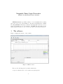
The software
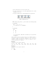
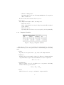
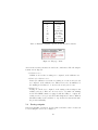
Figure 1 displays the interface of the software.
Figure 1: LFL Forecaster
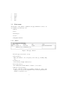
There are the following four icons in the main menu:
• Open icon that is used to select a time series (file upload)
1
• Save icon that is used to save the forecasts to files
• ZoomFit icon that is used to zoom-out the graph if it has been zoomed-in
manually by mouse before
• Compute icon that is used to run the implemented forecast methods.
Figure 2: Main menu icons
LFLF software package allows to open the text files of the following formats
1. # Comment
Title 66 70 74 63 . . .
i.e., the data is in a row. See Example 1.
or
2. # Comment
Title
1
66
2
70
3
74
4
63
..
..
.
.
i.e., the data is in the column where each value is preceded by its index.
See Example 2.
Title is a name of a time series that is followed by an unlimited number of
real numbers delimited by a blank space (TAB, space, etc.). Comment is a
description of a time series that is preceded symbol # delimited by a space.
Comment and Title are not obligatory.
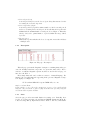
Example 1
# Monthly car sales in Quebec 1960-1968
Car sales 8728 12026 14395 14587
9545 7237 9374 11837 13784 15926
Example 2
# Monthly car sales in Quebec 1960-1968
Car sales
1
8728
2
12026
2
13791
13821
9498
11143
8251
7975
7049
7610
3
4
5
6
7
8
14395
14587
13791
9498
8251
7049
1.1
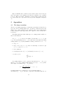
Main menu
The interface of the software contains five tab-pages which serve a user to set
up details for a prediction process:
• Global
• View
• Trend Cycle
• Season
• Linguistic Variables
1.1.1
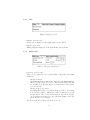
Global
Figure 3: Tab-page “Global”
Global tab-page serves users to set up:
• Data frequency
This option allows to choose frequency of the data (e.g. monthly, daily,
etc.)
• Validation set
A user sets up a length of this set here.
• Forecasting horizon
Forecasting horizon is the number of values to be forecasted.
• Check-box Cut-off Testing
It can be ticked if a testing set is available. In this case, values of the
testing set are not used for computation. These data are purely used for
evaluation of prediction error.
3
1.1.2
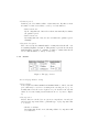
View
Figure 4: Tab-page “View”
• Check-box Trend-Cycle
Trend-cycle is displayed on the graph if this option is ticked.
• Check-box Partition
Fuzzy partition is displayed on the graph if this option is ticked.
1.1.3
Trend Cycle
Figure 5: Tab-page “Trend Cycle”
• Linguistic predictor type
There are two ways how to forecast the future components of the fuzzy
transform:
– Check-box Simple
By ticking this check-box the next component of the fuzzy transform
will be forecasted from previous n components and their first and
second differences. It means that we forecast from forecasted values
(one step ahead).
– Check-box More steps ahead
By ticking this check-box one may avoid the problem of “forecasting
from forecasted values”. This is due to the construction of several
independent models: one model forecasts one step ahead, another
one forecasts two step ahead etc. up to the desired number of models
(steps ahead to be forecasted).
If both are ticked the software selects the better one.
4
• Partition period
Partition period determines width of basic functions. By this we mean
the number of time series values covered by one basic function.
– Radio button auto
By choosing this radio button the software automatically determines
the partition period.
– Radio button user
By ticking this radio button a user determines the partition period
manually.
• Linguistic description
Here a user sets up the minimal number of fuzzy rules that should occur
in a winning linguistic description. This parameter prevents an extremely
small linguistic description, consisting of number of fuzzy rules that is
below a critical number, to win (to be selected).
1.1.4
Season
Figure 6: Tab-page “Season”
Season tab-page allows to set up:
• Season depth
Season depth determines minimal and maximal number of whole seasonal
period that may be used for forecasting next seasonal period (e.g. for
monthly time series the season depth is one year and the next seasonal
values are forecasted using seasonal values from 1 to 4 years, see Figure
6).
• Decomposition
Models, that are searched for, are given as compositions of trend-cycle
and seasonal components. Hence, particular type of (de)composition has
to be chosen.
– Check-box Additive
By ticking this check-box models using additive decomposition will
be searched for.
5
– Check-box Multiplicative
By ticking this check-box models using multiplicative decomposition
will be searched for.
If both are ticked the software selects better one.
• Periodicity
Periodicity is the length of whole seasonal period.
– Radio button auto
By choosing this radio button periodicity is automatically determined
by the software.
– Radio button user
By ticking this radio button a user sets up the periodicity manually.
1.1.5
Linguistic Variables
Figure 7: Tab-page “Linguistic Variables”
This tab-page allows to set up minimal and maximal numbers of the input
variables that may occur among antecedents of automatically generated fuzzy
rules.
• Value
By values we directly mean the components of the fuzzy transform.
• Difference
In this block we set up a number of first order differences of fuzzy transform
components that are given as follows differences between components
∆Xi = Xi − Xi−1
• 2nd Difference
These are values of second order differences of components of the fuzzy
transform that are given as follows
∆2 Xi = ∆Xi − ∆Xi−1
• Total
This block is used to set up a total number of input variables.
6
1.2
Outputs
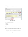
Figure 2 displays the interface of the LFLF after a time series is forecasted.
Figure 8: LFL Forecaster
There is a windows with three tab-pages in the right bottom area of the
interface. These tab-pages, particularly:
• Features
• Description
• Stats
display distinct information related to the results, used models, measured errors
etc.
1.2.1
Features
This tab-page presents the main features of a winning model, see Figure 9. It
contains the following features:
• Trend-cycle type
Trend-cycle type determines the method that was used for modelling the
trend-cycle.
7
Figure 9: Tab-page “Features”
(Remark: So far, the inverse fuzzy transform denoted by “inverse FT” is
the only method that is at disposal. The LFLF is ready to be enriched by
other methods.).
• Partition period
Partition period displays the partition period of the winning model, i.e.,
the number of time series values that is covered by any basic function of
the model that is used to describe and forecast a given time series.
• Predictor type
Predictor types describes whether Simple (denoted by the word “Linguistic”) or More steps ahead (denoted by “Steps ahead linguistic”) trend-cycle
prediction was used.
(Remark: The LFLF is ready to be enriched by other methods hence the
word “linguistic” appear in the trend-cycle predictor name.)
• Variables
This feature displays antecedent and consequent variables that appear in
fuzzy rules describing the trend-cycle model. Particularly, S denotes the
trend-cycle components, dS their differences and d2S their second order
differences. The argument (t), (t − 1),etc. denotes the time lag of the
component.
For example, taking S(t)&dS(t) → dS(t + 1) from Figure 9 denotes the
fact that Xi and ∆Xi are the antecedent variables and ∆Xi+1 is the
consequent variable of the winning model and hence, we deal with rules
of the form:
IF Xi is Ai AND ∆Xi is A∆i THEN ∆Xi+1 is ADeltai
• Season type
This feature denotes the model (and consequently the method) that is
used to forecast seasonal components.
(Remark: So far, only the “LMS linear combination” method that assumes
an entire seasonal period to be a linear combination of previous periods.
The LFLF software is ready to be enriched by other methods.)
8
• Seasonal periodicity
Seasonal periodicity denotes the detected periodicity that was used for the
forecasting the seasonal component.
• Season dependency depth
Seasonal dependency depth determines number of whole seasonal periods
used for forecasting next seasonal periods. Recall, that users specifies the
minimal and the maximal number of such periods, see Figure 6. This value
already denotes the optimal number of periods within the range defined
by a user.
• Decomposition
This feature specifies whether the chose decomposition was either Additive
or Multiplicative.
1.2.2
Description
Figure 10: Tab-page “Description”
This tab-page presents the linguistic description containing fuzzy rules generated from fuzzy transform components of a given time times series. Abbreviations of evaluative linguistic expressions, that are used in the tab-page, are
introduced in Table 1.
Every single fuzzy rule can be taken as a sentence of natural language. For
instance, the very first fuzzy rule appearing in the generated linguistic description displayed on Figure 10:
IF Xi is ml sm AND ∆Xi is qr sm THEN ∆Xi+1 is −me
may be read as follows:
If the number of cars sold in the current year is more or less small and the
half-year sales increment is quite roughly small then the upcoming half-year
increment will be negative medium.
1.2.3
Stats
Stats tab-page provides users with distinct forecasting error. Basically, there
is only one accuracy measure, the well known SMAPE (Symmetric Mean Absolute Percentage Error), implemented in the software so far. Note, that further
9
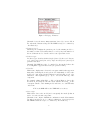
Abbreviation
sm
me
bi
ve
si
ex
ml
ro
qR
vR
Ev.expression
small
medium
big
very
significantly
extremely
more or less
roughly
quite roughly
very roughly
Table 1: Evaluative linguistic expressions and their abbreviations
Figure 11: Tab-page “Stats”
criterions and accuracy measures are under the consideration. The following information is at disposal:
• Validation error
Validation error is the forecasting error computed on the validation set.
• Trend-cycle validation error
Trend-cycle validation error is the forecasting error of the trend-cycle values computed on the validation set. This serves for the determination of
the winning model that is to be used for the trend-cycle forecast.
• Testing error
Testing error is the error computed on the testing set if a testing set was
available and used. This error is never used to determine the winning
model! The LFLF software is equipped with the ability to compute the
testing error in order to provide users with a high users comfort. Without
this functionality, users would have to export their forecasts and measure
the precision manually.
1.3
Saving outputs
Generated linguistic description, model features and time series forecasts can
be saved using the Save icon, see Figure 2.
10
Exported MS Excel file contains forecasted values, values of the trend-cycle
and some features of the winning model such as a validation error, partition
period etc. Exported text file contains the forecasted values of a time series, the
forecasted trend-cycle components, trend-cycle predictor (linguistic description)
etc.
2
Appendixes
2.1
The fuzzy transform
The idea of the fuzzy transform is to transform a given function defined in one
space into another, usually simpler space, and then to transform it back. The
simpler space consist of a finite vector of numbers. The reverse transform then
leads to a function, which approximates the original one. More details can be
found in [3].
The fuzzy transform is defined with respect to a fuzzy partition, which consists of basic functions.
Let c1 < · · · < cn be fixed nodes within [a, b] such that c1 = a, cn = b and
n ≥ 2. We say that fuzzy sets A1 , . . . , An ∈ F([a, b]) are basic functions forming
a fuzzy partition of [a, b] if they fulfill the following conditions for i = 1, . . . , n:
1. Ai (ci ) = 1;
2. Ai (x) = 0 for x 6∈ (ci−1 , ci+1 ), where for uniformity of notation we put
c0 = c1 = a and cn+1 = cn = b;
3. Ai is continuous;
4. Ai strictly increases on [ci−1 , ci ] and strictly decreases on [ci , ci+1 ];
5. for all x ∈ [a, b],
n
X
Ai (x) = 1.
i=1
Let a fuzzy partition of [a, b] be given by basic functions A1 , . . . , An , n ≥ 2
and let f : [a, b] → R be a function that is known on a set {x1 , . . . , xT } of points.
The n-tuple of real numbers [F1 , . . . , Fn ] given by
PT
Fi =
t=1 f (xt )Ai (xt )
,
PT
t=1 Ai (xt )
i = 1, . . . , n,
is a fuzzy transform of f with respect to the given fuzzy partition.
The numbers F1 , . . . , Fn are called the components of the fuzzy transform of f .
11
Let Fn [f ] be the fuzzy transform of f with respect to A1 , . . . , An ∈ F([a, b]).
Then the function fF,n given on [a, b] by
fF,n (x) =
n
X
Fi Ai (x),
i=1
is called the inverse fuzzy transform of f .
2.2
Linguistic description (fuzzy IF-THEN rules)
Fuzzy IF-THEN rules can be understood as a specific conditional sentence of
natural language of the form
IF X1 is A1 AND · · · AND Xn is An THEN Y is B,
where A1 , . . . , An and B are evaluative expressions (very small, roughly big,
etc.). An example fuzzy IF-THEN rule is
IF the number of cars sold in the current year is more or less small and the
half-year sales increment is medium THEN the upcoming half-year increment
will be medium.
The part of the rule before THEN is called the antecedent and the part after
it is called the consequent.
Fuzzy IF-THEN rules are usually gathered in a linguistic description
R1 := IF X1 is A11 AND · · · AND Xn is A1n THEN Y is B1 ,
...................................
Rm := IF X1 is Am1 AND · · · AND Xn is Amn THEN Y is Bm .
2.3
Perception-based logical deduction
Perception-based logical deduction (PbLD) is a special method of deducing conclusions on the basis of a linguistic description. This method can be described
as follows: if a linguistic description consisting of fuzzy IF-THEN rules together
with an observation of some value of the variable X are given, then the PbLD
chooses the most specific fuzzy rule(s) among the most fired ones and derives a
conclusion based on such preselected fuzzy rule(s). More details can be found
in [2] or in [1].
2.4
Implementation of these techniques
Let time series xt , t = 1, . . . , T is viewed as a discrete function x on a time axis
t. Then Fn [x] = [X1 , . . . , Xn ] is the fuzzy transform of the function x with
respect to a given fuzzy partition. The inverse fuzzy transform then serve us as
a model of the trend-cycle of a given time series. By subtracting the trend-cycle
(inverse fuzzy transform) values from the time series lags, we get pure seasonal
12
components. This is how the fuzzy transform helps us to model and decompose
a given time series.
Logical dependencies between components X1 , . . . , Xn of the fuzzy transform
may be described by the fuzzy rules. These rules are generated automatically
from the given data and are used for forecasting the next components. Fuzzy
transform components as well as their first and second order differences are used
as antecedent variables. For forecasting future fuzzy transform components
based on the generated fuzzy rules, a special inference method – perceptionbased logical deduction [2] – is used. This is how fuzzy rules and the PbLD are
implemented in the software.
The seasonal components are forecasted autoregressively. Finally, both forecasted components – trend-cycle and seasonal – are composed together to obtain
the forecast of time series lags.
References
[1] V. Novák, M. Štěpnička, A. Dvořák, I. Perfilieva, V. Pavliska and L.
Vavřı́čková, 2010. Analysis of seasonal time series using fuzzy approach,
International Journal of General Systems, 39, 305–328.
[2] Novák, V. and Perfilieva, I., 2004. On the Semantics of Perception-Based
Fuzzy Logic Deduction. International Journal of Intelligent Systems, 19,
1007–1031.
[3] Perfilieva, I., 2006. Fuzzy Transforms: theory and applications. Fuzzy Sets
and Systems, 157, 993–1023.
[4] M. Štěpnička, A. Dvořák, V. Pavliska and L. Vavřı́čková, 2010. Linguistic
approach to time series analysis and forecasts. Proc. FUZZ-IEEE, 2149–
2157.
13