1
University of Twente
EEMCS / Electrical Engineering
Control Engineering
Characterization of the mVSA-UT
H.W. (Han) Wopereis
BSc Report
Committee:
Prof. dr. ir. S. Stramigioli
Dr. R. Carloni
Dr. ir. P. Breedveld
M. Fumagalli, PhD
Dr. ir. R.J. Wiegerink
August 2012
Report nr. 019CE2012
Robotics and Mechatronics
EE-Math-CS
University of Twente
P.O. Box 217
7500 AE Enschede
The Netherlands
Contents
1 Introduction
1.1 Project goal . . . . . . . . . . . . . . . . . . . . . . . . . . . . . .
1.2 Report outline . . . . . . . . . . . . . . . . . . . . . . . . . . . .
4
5
5
2 Requirement and approach analysis
2.1 Approach options analysis . . . . . . . . . . . . . . . . . . . . . .
2.2 General requirements . . . . . . . . . . . . . . . . . . . . . . . . .
2.3 Detailed approach analysis . . . . . . . . . . . . . . . . . . . . . .
6
6
8
8
3 Electronic part of the measurement setup
3.1 Strain gauges . . . . . . . . . . . . . . . . .
3.2 8-channel amplifier board . . . . . . . . . .
3.2.1 Requirements . . . . . . . . . . . . .
3.2.2 Analysis . . . . . . . . . . . . . . . .
3.2.3 Design . . . . . . . . . . . . . . . . .
3.3 Motors and motor drivers . . . . . . . . . .
3.4 Arduino ATMEGA2560 . . . . . . . . . . .
.
.
.
.
.
.
.
.
.
.
.
.
.
.
.
.
.
.
.
.
.
.
.
.
.
.
.
.
.
.
.
.
.
.
.
.
.
.
.
.
.
.
.
.
.
.
.
.
.
.
.
.
.
.
.
.
.
.
.
.
.
.
.
.
.
.
.
.
.
.
.
.
.
.
.
.
.
.
.
.
.
.
.
.
10
10
11
11
12
13
15
15
4 Mechanical part of the measurement setup
4.1 Sensor analysis . . . . . . . . . . . . . . . .
4.1.1 Options research . . . . . . . . . . .
4.1.2 Sensor design using FEM analysis .
4.2 Setup design . . . . . . . . . . . . . . . . .
4.2.1 Materials and components . . . . . .
.
.
.
.
.
.
.
.
.
.
.
.
.
.
.
.
.
.
.
.
.
.
.
.
.
.
.
.
.
.
.
.
.
.
.
.
.
.
.
.
.
.
.
.
.
.
.
.
.
.
.
.
.
.
.
.
.
.
.
.
16
16
17
19
21
26
5 Measurements
5.1 Calibration . . . . . . . . .
5.1.1 Calibration principle
5.1.2 Calibration results .
5.2 Measurements and analysis
5.3 Improvement analysis . . .
5.4 Data extraction . . . . . . .
5.5 Results . . . . . . . . . . . .
.
.
.
.
.
.
.
.
.
.
.
.
.
.
.
.
.
.
.
.
.
.
.
.
.
.
.
.
.
.
.
.
.
.
.
.
.
.
.
.
.
.
.
.
.
.
.
.
.
.
.
.
.
.
.
.
.
.
.
.
.
.
.
.
.
.
.
.
.
.
.
.
.
.
.
.
.
.
.
.
.
.
.
.
27
27
29
29
31
34
35
36
.
.
.
.
.
.
.
.
.
.
.
.
.
.
.
.
.
.
.
.
.
.
.
.
.
.
.
.
.
.
.
.
.
.
.
.
.
.
.
.
.
.
.
.
.
.
.
.
.
.
.
.
.
.
.
.
.
.
.
.
.
.
.
6 Conclusion and recommendations
39
A Paper of the mVSA-UT
41
B B: The 8-channel Amplifier board user’s manual
49
2
C C: Data-sheets
76
D D: Solid-works drawings
77
E E: Matlab files
88
E.1 File used to extract single data values . . . . . . . . . . . . . . . 88
E.2 File used to extract the final matrices from all measurement data 94
F F: Measurements data
98
F.1 Final measurement data . . . . . . . . . . . . . . . . . . . . . . . 99
F.2 Verification data . . . . . . . . . . . . . . . . . . . . . . . . . . . 101
3
Chapter 1
Introduction
One of the latest researches in the field of robotics is the research on variableimpedance-actuators. These are actuators with adjustable compliance and damping, which can store and release mechanical energy. This can be used for soft
and energy-efficient interaction with the environment, giving a certain degree of
safety.
One of the research collaborations focused on this
is research is the VIACTORS-group [1].
The
viactors-group developed multiple different variable
impedance actuators [2], [3], [4], [5], and one of the
latest developments is the development of the miniaturized Variable Stiffness Actuator by the viactorsdivision at the university of Twente [6], which is
shown in figure 1.1. From here on the miniaturized
Variable Stiffness Actuator is referred to as mVSAUT. The mVSA-UT is a miniaturized version of the
VSA-UT [7], developed by the same research group.
The mVSA-UT is actuated using two motors, connected to a differential stage, to both rotate the output shaft and change the stiffness of this output.
The stiffness of the mVSA-UT can be changed by
moving a pivot point along a lever. This is illustrated in figure 1.2. The outer frame can be rotated
(Θ7 ) and the inner gear can be moved around o with
radius l. These are the two movements can be actuated by the two input motors.
Figure 1.1: A picture
of the newly developed
mVSA-UT, with a two
euro coin for size reference.
The novelty of the mVSA-UT and of the VSA-UT, lies in the possibility to vary
the stiffness of the output shaft from zero to almost infinite, while retaining a
wide (60o ) maximum deflection for zero stiffness settings. The novelty of the
mVSA-UT is its small size, which creates great possibilities for implementation
in smaller and more precise, compliance requiring, devices.
4
If the reader is unfamiliar with the conceptual design of the mVSA-UT, it is
recommended to at least read chapter III of paper [6]. This paper is added in
appendix A.
1.1
Project goal
The main goal of this project is to
contribute to characterizing the mVSA
by determining its internal dissipation.
The results of this project could then be
used in modeling of the mVSA. This has
to be done with a low budget and thus
expensive measurement systems cannot
be bought. The measurement equipment therefore has to be developed and
debugged within the project.
P1
Fo
d7
Peq
0
Fs
θ2
l
θ6
Po
θ1
Pp a
Fp
Ps
1.2
P2
Report outline
θ7
This report will be split up into three
main chapters, since the assignment was Figure 1.2: One of the internal levels
as well mainly split into 4 parts: analy- of the mVSA-UT, showing the differsis of the problem, designing and build- ential connection to the pivot point.
ing the electronics, designing and building a mechanical setup and performing
measurements and data analysis.
First, in Chapter 2 an analysis of
the main requirements to achieve the
project goal is given and the options on achieving this goal are discussed. Then
in Chapter 3 the development of the electronic data collecting board is described, as well as the other electronics used for the measurement setup. In
Chapter 4 an outline is given on the development and realization process of the
mechanical part of the measurement setup. Chapter 5 discusses the process for
taking measurements and the results. Finally in Chapter 6 the conclusions and
recommendations are discussed.
5
Chapter 2
Requirement and approach
analysis
To achieve the main goal, determining the dissipation of the mVSA-UT, an
measurement setup has to be build. Therefore requirements on such setup have
to be analyzed. In this chapter the requirements, from the goal’s point of view,
are given. More specific requirements on specific aspects of the to-be-build
measurement setup are given in (sub)sections of the relevant chapters.
2.1
Approach options analysis
Determining the internal dissipation of the mVSA-UT can be done by measuring
the power put into the system in steady state and compare it to the power that
is taken at the output. The difference is the power loss inside the system.
The easiest way to measure this loss is by setting the power withdrawn from
the output to zero. In that case all power supplied to the system is used to
overcome internal energy losses.
Thus a way to determine the input power of both inputs has to be found. Since
the input power of each input is given by (2.1), with τ being the delivered
torque in N · m and ω being angular velocity in rad · s−1 , the input power can
be determined when measuring both the velocity and torque applied to each
input shaft. Since measuring angular velocity is fairly easy using encoders, the
main approach issue is how to measure the input torque.
Pin = τin · ωin
(2.1)
One method to determine the input torque can be to characterize the servos
used to actuate the mVSA-UT. To do this, a setup has to be created that can
6
determine the output torque of the servos at certain applied currents. Using
this setup the relation between the current through the motor and the output
torque of the motor can be determined. Then by measuring the current that
passes through both the servos, while attached to the mVSA-UT, the torques
applied to the inputs can be found.
While this can be done, the question is how accurate the measurements will
be. It is highly probable that the servos are not robust and better motors are
needed. Furthermore it is expected that a setup built to characterize motors
supplying 100 Nmm of torque will probably give an inaccurate characterization
for torques below 10 Nmm. In other words, the setup will be less adaptable. In
order to create the best possible setup it is therefore necessary to have a good
estimation of the torques that will be applied to the mVSA.
Another method is to create a dynamic torque sensor setup. This setup is
placed in between a motor and one of the inputs of the mVSA-UT. Using the
torque sensor, as the name states, the input torque applied to the mVSA-UT
can directly be measured. The torque sensor could either be bought or designed
and built.
The advantages of this option are that the measurement setup is highly adaptable and it is straight-forward to build. Depending on the properties of the
torque sensor, fairly great ranges of torques could be measured with high precision with only minor adaptations of the setup. The disadvantage of this option
is that the sensor rotates along with the input shaft. Thus a solution has to be
found for the wires going to the sensor. Also, if the sensor is not well calibrated,
there could be noise from the rotation. Therefore, the calibration has to be done
accurate.
Then there is also the option of creating a static torque sensor setup. This setup
measures the reaction torque the motor induces when applying a torque to the
mVSA-UT. This torque sensor to which the motor is connected can as well be
either bought or designed and built.
The advantage of this option is again adaptability, however it is less adaptable
than the previous option. The precision will depend on the properties of the
sensor. The disadvantage of this option is that the sensor has to carry the
motor, which can lead to cross-talk errors. Also carrying the motor could give
reduced sensitivity, as the sensor has to be over-sized to carry the extra load.
7
Table 2.1: List of advantages and disadvantages of three approach options.
Approach option
Characterize
motors
Advantages
Disadvantages
Once motors are characterized properly, measuring is easy
Dynamic torque
sensor setup
Static
torque
sensor setup
High adaptability - Precision depending on sensor
Medium-high adaptability
- Precision depending on
sensor
Requires better motors Low adaptability - Precision depending on motor
and characterization
Rotating sensor could give
problem with wires
Possibility of cross-talk Possibility of reduced sensitivity
Comparing all advantages and disadvantages in table 2.1, the choice is made
for the second option, the dynamic torque sensor setup. The accuracy of the
measurement has to be precise, which excludes the option to characterize the
servos. Although this option can be precise, there are a lot of uncertainties
which could give problems. When comparing the second and third options, the
static torque sensor setup possibly generates more noise in the measurements
and could give a reduced sensitivity. These disadvantages outweigh the possible
problem with the wires of the dynamic torque sensor setup.
2.2
General requirements
The general requirements towards achieving the main goal are given in section
1.1. The internal dissipation has to be determined by creating a low budget
measurement system. The dimension of torques to measure is unknown and
therefore it is hard to give an exact requirement on the precision of the measurement system. The precision therefore has to be as high as possible with the
resources available and precise enough to achieve the main goal. The frictional
torques to measure are expected to be within the range of 1 − 100N mm.
2.3
Detailed approach analysis
To determine the internal dissipation of the mVSA-UT it is necessary to know
what kind of results to expect. Since the mVSA-UT is actuated by two servos
connected through a differential stage, the dissipation of both the rotational
output as the movement of the pivot point will depend on both input velocities.
It is assumed that the dissipation can be approximated as linear dependent
on the input rotational velocities. If this is not a correct approximation, the
measurements will show this and the assumption has to be adjusted. Relation
(2.2) can be found between input velocities and measured torques in case of
8
linearity. Constants C1 and C2 in this equation are positive if the directions
of ω1 and respectively ω2 are positive, and negative when the directions are
negative.
C1
C3
C2
dir(ω1 )
a
·
+
C4
dir(ω2 )
c
b
ω
τ
· 1 = 1
d
ω2
τ2
(2.2)
One possibility to gather the values of the two matrices is by taking a lot of
measurements and finding the values that best fit to those measurements. These
measurements can be done by building a setup that contains two torque sensors.
Since torque sensors are usually quite expensive to buy, these have to be designed
and build within the project.
The torque sensors can be designed using strain gauges. The most commonly
used strain gauges are foil gauges and semiconductor gauges [8]. Since the strains
are expected to be very small, the semiconductor strain gauges seem to be the
best choice. These have higher resistance values and bigger sensitivity compared
to foil gauges, but also have greater sensitivity to variations in temperature and
the tendency to drift when aging. The advantages outweigh the disadvantages,
since the temperature is going to be approximately constant while measuring
and the measurements are only done in a relatively short period of time.
The applied input torques can be found by creating a sensor that connects one
side of the setup, where the motor is located, to the other side, of the mVSAUT, using small cantilevers. The strain of these cantilevers can be measured by
using a Wheatstone full bridge configuration of strain-gauges. A full bridge is
used since this will give the most sensitivity.
To be able to measure the voltages coming from the two full bridges with high
precision, additional electronics are necessary. These electronics have their own
requirements, which are described in section 3.2.2.
To determine the optimal shape of the torque sensor and to fit the cantilevers
to the expected range of torques to be measured, finite element method (FEM)
analysis has to be done.
After the shape and dimensions of the sensor are determined, it is necessary
to create a setup that connects the motor, sensor and mVSA-UT. This setup
should influence the measurements as little as possible and has to guarantee a
high adaptability.
When the setup is designed and build, the sensors have to be calibrated. This
can be done with a torque sensor, which was bought for another project, thus
saving expenses. After calibrating the setup, it can be used to do the measurements.
9
Chapter 3
Electronic part of the
measurement setup
This chapter will cover the strain gauges and electronics used in the torque measurement setup. The 8-channel-amplifier-board, designed within this project
will be presented, as well as a summary of the other electronics used in the
measurement system.
3.1
Strain gauges
It was discussed in section 2.3 that semiconductor strain gauges were the best
choice for this project. The semiconductor strain gauges used were purchased
at Micron Instruments. The ”U” shaped SS-037-022-500PU strain gauges were
selected. These are smaller and have better thermal coefficients than most
others. The in rest resistance of these strain gauges is 540Ω with a maximal
variation in resistance of 50 Ohms.
These strain gauges are selected because of the big linear region. The strain
1
gauges have a linearity better than 0.25% to 600µ mm
mm which is approximately 5
mm
of the full range and a linearity better than 1.5% to a strain of 1500µ mm which
is half of the full range. They also have been selected because of the small size.
10
3.2
8-channel amplifier board
This section of the report describes the development process of the 8-channelamplifier-board, referred to as 8AMP from here on, used for the measurement
setup. It gives the criteria and design choices for the 8AMP, as well as a brief
description of the design process. For more information, an users manual is
included in appendix B. This manual provides, among others, more specific
information on the design of the 8AMP and a bill-of-materials. It also includes
an extensive programming guide for the 8AMP, using the Arduino-Bootloader.
3.2.1
Requirements
To create a good design, the requirements have to be known. The requirements
that are needed for the torque sensor setup are:
1. At least two inputs able to measure differential voltages or at least four
inputs to measure non-differential voltages.
2. A data collecting frequency of at least 100 Hz for each channel and the
data has to be converted to digital signals.
3. An amplifier and low-pass-filter are required. The amplifier gain has to
be adaptable depending on the range of different input-voltages.
4. The board itself has to provide power to the strain gauges.
The first requirement is defined by the chosen approach 2.3. The second is due
to the fact that low frequency signals, below 20 Hz, should be clearly visible in
the measurement results. The third requirement is made because the expected
strains to be measured, and thus the expected voltage range, is not well known.
If it is the case that, for example, only 15 th of the total voltage range of the
analog-to-digital-converter (ADC) is used, which will decrease the accuracy of
the ADC by at least 2 bits, this should be easily changed. The last requirement
is necessary to ensure the voltages applied to the strain gauges are matched.
The electronics created in this project to measure the strain gauge bridges will
also be used in another project, the manipulator of the Airobots group [9], [10].
This manipulator will eventually be attached to the a Quadrotor Unmanned
Aerial Vehicle. The manipulator will use strain gauges to take joint-torque or
6-dimensional(D) force-torque measurements.
This extra application brings forth some extra requirements, listed below:
4. The board should have at least 6 half-bridges inputs for 6D force-torque
measurements.
5. The weight should be as low as possible.
11
6. The information processing should be done on-board.
7. Communication protocol should be either CAN or Serial.
Since the board is going to be used on a flying robot, the weight should not
be too high. Because the processing power of the processor of the manipulator
has to be used for doing other calculations, the data-collecting and transmitting
of the 8AMP has to be done by an on-board processor. This processor then
communicates with the other processor, either by CAN or Serial communication.
3.2.2
Analysis
To build an electronic board that can achieve the given requirements 3.2.1, the
correct components have to be found. The choice has been made to use a single
supply voltage for the 8AMP of 5 volts. This voltage provides the most options
in selecting components and is commonly used for this kind of electronics.
All the links to the data-sheets of the main components can be found in appendix
C.
To meet the requirements, the choice has been made to use a multiplexer to
pass up to 8 different input signals to an amplifier. The amplifier amplifies
the data of one of the 8 different input signals and passes this amplified value
towards an ADC. The ADC is controlled by a micro-controller, as well as the
multiplexer. After conversion the ADC passes the digital value to the microcontroller, which on its turn, presents the value on either the Serial line or to
the Serial-to-CAN-transceiver.
The multiplexer chosen for this application is the Maxim DG408DY. This multiplexer is capable of multiplexing between 8 different channels, by setting three
pins of logic to either ON or OFF. The advantages of this multiplexer are the
small package (16 narrow SO) and the fast transition time (250ns). The transition time is the time needed to switch between channels. Although the ONresistance of this multiplexer is quite high (±100Ω), this will not provide any
problems, since the input impedance of the selected amplifier, described below,
is extremely high (1010 Ω).
The INA118-UB is selected as amplifier for this application. This amplifier
is a general purpose amplifier offering excellent accuracy. The amplifier can
amplify signals using only a single power supply, comparing the input signal to
a reference signal. In this application, the voltage supplied to the strain gauge
half-bridges will be 5 volts. Assuming the half-bridges are balanced, a strain of
0 mm/mm will return a voltage of 2.5 volts. The reference of the INA118-UB
will be set to 2.5 volts, while matching the impedance of the strain gauge halfbridges using thin-film resistors. These resistors introduce less thermal noise
into the system. When a strain is applied to the strain gauges, the bridges
will not balanced anymore. The voltage returned will now be different from 2.5
volts, e.g. 2.2 volts. The amplifier will compare this voltage to the reference
and detect a difference of 0.3 volts. This difference is then amplified by the
12
gain-factor, subtracted from the reference voltage and presented at the output.
In case of a difference of 0.3 volts and a gain factor of 5, the voltage at the
output will now be 1 volts.
V
Other crucial features of the INA118 are the high slew-rate (0.9 µs
), low gain error, small package (SOIC-8) and the possibility to set the gain using an external
resistor. The formula to set the gain is given by equation (3.1).
G=1+
50kΩ
Rg
(3.1)
Rg being the external resistor. This external resistor should not produce to
much thermal noise and thus thin-film resistors will be used for Rg .
The ADC chosen is the ADS7279. This low-power, 14-bit analog-to-digital
converter has a sampling rate of 1 MHz. It has been selected because of the
high accuracy (14 bits - max 1 LSB1 ), small package (TSSOP-16), unipolar input
and the fast sampling rate. Since the footprint is the same as the ADS8329,
the accuracy of (14-1) bits can even be increased to (16-1) bits, but this is not
necessary for this application. The accuracy in volts, when using a power supply
of 5 volts and assuming a precision of 13 bits is 0.625 mV, which is considered
accurate enough.
The micro-controller chosen to operate the ADC and the multiplexer is the ATMEGA328PA. This micro-controller has been chosen mainly due to its compatibility with the Arduino software. With the Arduino-bootloader being available
for this type of micro-controller, the coding can be done in the easier-to-use
Arduino environment and re-uploading code can be done through serial communication instead of using an In-Serial-Programmer. An external clock source
of 16 MHz is used to achieve double the processing power compared to the
internal clock of 8 MHz of the ATMEGA328PA.
The ATmega328P uses a serial interface to communicate with either the user
(computer) or another microprocessor. To also have the option to use CANcommunication, the SN65HVD1050D from Texas Instruments has been selected
as Serial-to-CAN transceiver. This is an extra option of the board, which will
not be further discussed anymore.
Next to these components, there will be some LEDs indicating whether the
power is on, a reset is initiated and if the communication is active.
3.2.3
Design
The complete schematic of the 8AMP is well-explained in the manual in appendix B and thus will not be explained again here.
1 LSB stands for least significant bit. In this case only the least significant bit is considered
to be noise. This is normal, since the last bit always rounds of the final residue and is thus
not completely accurate
13
The printed-circuit-board (PCB) design process of the 8AMP is also described
in the manual. A short summary on the design: The 8AMP is a 4-layer PCB.
It has carefully be designed to have as low noise on signal wires as possible.
Digital and analog signals are separated. Signal wires are as short and straight
as possible and wiring at different layers is oriented in perpendicular directions
where possible. Capacitors, ferrite-beads and coils are used for filtering the
power supply of different components. Ground planes are used on each layer
to decouple noise and cross-talk between adjacent wires and to ensure the same
reference potentials.
The final PCB is shown in figure 3.1 with the components soldered to the
board (except for the Serial-to-CAN-transceiver). The dimensions are x x mm
and the total weight including components is X grams. It contains five LEDs,
indicating: power, reset, transmit, receive and clock. The clock indicates if the
ADC is transferring data to the micro-controller. The 8AMP can be connected
to another PCB with as little as 4 wires: power, ground, RXD (or CANLOW )
and TXD (or CANHIGH ). There is however an additional connector located at
the 8AMP, which can be used to program the ATmega328P using an In-Serialprogrammer. The 8AMP has 24 pads, 8 x 3 pads, which supply power and
ground towards strain gauge half-bridges, and extract the signal.
Figure 3.1: A photograph of the 8-channel amplifier board (8AMP).
To connect the 8AMP directly to a PC, a Serial-To-USB transceiver is required.
The transceiver chosen in this project is the UB232R module by FTDI Chip.
The link to the data-sheet of this manual can be found in appendix C.
14
3.3
Motors and motor drivers
The motors that will be used initially
are two MAXON RE10 DC motors
with GP10A (four stage 256:1) reduction gears and with MEnc10 12 ticks
magnetic encoders which are readily
available but broken. The encoders
of these motors were both broken,
but could be repaired by removing
and reconnecting the magnetic sensors. These magnetic sensors either
had loose connections or where bent,
resulting in bad encoder readings.
The motors can provide over 1.5
mNm of continuous torque when applying 6 volts, which results in more Figure 3.2: A photograph of the Pololu
than 200 mNm of torque at the out- 755 motor driver completely assembled.
put of the gearbox. This is expected
to be more than sufficient to drive the
measurement setup. The rotational velocity of the output shafts of these motors
is however quite low (< 8rpsif Vm = 6V ) due to the reduction gears. But since
these motors are available, these will be used.
The motor-drivers used to supply power to these motors are two Pololu 755
High-Power Motor Drivers. Figure 3.2 displays a completely soldered board.
This discrete MOSFET H-bridge motor driver provides bidirectional control for
one brushed DC motor. The motors are powered with 6 volts (at least 5.5 V
is necessary), which has to be separately provided to the motor driver. More
information on this motor driver can be found on the website of Pololu [11].
3.4
Arduino ATMEGA2560
For communication between the PC (user), the 8AMP board and the two Pololu
boards, an Arduino Mega 2560 with an Atmel ATmega2560 processor is used.
It runs custom made firmware which takes care of communication with the PC,
sending PWM and direction signals to the motor drivers, reading the encoder
increment interrupts and receiving the torque measurement values from the .
The Arduino MEGA 2560 also provides power to the logic of the motor drivers
and the 8AMP board.
15
Chapter 4
Mechanical part of the
measurement setup
This chapter of the report covers the development of the mechanical aspects
of the measurement setup. The analysis of the sensor and the design of the
measurement setup are presented. Also the realization of the setup is described.
4.1
Sensor analysis
The principle used for the torque sensor is based on beam flexing. By connecting
the strain gauges to a cantilever, as displayed in figure 4.1, the impedance of
these strain gauges varies when applying an force at the end of the beam. This
variation can then be measured.
Figure 4.1: Principle used for torque sensor illustrated.
16
Below first some options for the shape are presented, from which the best one
for this application will be chosen. The correct dimensions for the sensor will
then be determined using the data-sheet of the semiconductor strain gauges and
FEM analysis. This will ensure that the sensor is able to measure the expected
range of strains using the maximum linear region of the strain gauges.
4.1.1
Options research
There are several different structures suitable for torque sensors. Some very
basic designs are the solid and hollow cylinders, like shown in figure 4.2. One
side of the sensor is connected to the motor and the other side to the mVSA-UT.
Figure 4.2: Basic designs for torque sensors. Solid cylinder is shown left, hollow
cylinder is shown right.
Then there are the more complex shapes, in the shape of hub-sprockets and
hollow cruciform which are shown in figure 4.3. The hub-sprocket has an inner
cylinder and an outer cylinder. One of them is connected to the motor and the
other to the mVSA-UT. The hollow cruciform is connected likewise as the solidand hollow cylinder.
Figure 4.3: More advanced designs for torque sensors. Left the hub-sprocket is
shown, right the hollow cruciform.
17
One advantage of the basic designs is that the sensors are easily produced, but
for the range of torques in this project the cylindrical shape would have to be
very small and the hollow shape very thin to assure full use of the sensitivity of the strain gauges, making it very fragile to non-torsional torques. Also
non-torsional components will not be permitted, since they can influence measurements.
The hub-sprocket design is more advanced, requiring more advanced production
methods. It can be build with any amount of cantilevers, but since the torques
are assumed to be very small, two cantilevers will be sufficient. This sensor,
in combination with a strain gauge full bridge, has the advantage that bending
moments, normal forces and perpendicular forces can be mostly filtered from
the strain gauge readings. The sensor with a strain gauge full bridge is shown
in figure 4.4. When a normal force in the z-direction or a non-torsial bending
moment is applied, all strain gauges will elongate an equal amount, thus there
is no difference in the output. When a perpendicular force is applied pointing
down in the y-direction, the top two strain gauges will shorten, while the two
bottom gauges elongate. In the ideal case, nothing will happen, since both halfbridges change the same way. In the less ideal case, if both half-bridges are not
completely balanced, these changes can be mostly removed by calibration. The
disadvantage of this shape, the drastic change in size, between the outer ring
and the inner ring, is no problem in this setup.
The hollow cruciform shape again has
a certain amount of cantilevers that
are bent due to applied torques. However, this shape requires even more
advance production methods. This
shape of torque sensors are more often
used in, for instance, robot joints. To
achieve good sensitivity, the stiffness
of these shapes has to be low and nontorsional torques have to be small. If
used in for instance a robot joint, the
sensitivity can be set lower, making
it stiff enough for a weight carrying
[H]
joint.
Figure 4.4: Illustration of hub-sprocket
Comparing all advantages to the distorque sensor design with two canadvantages, the hub-sprocket design
tilevers and a strain gauge full-bridge.
clearly is the best design for this
project. Its disadvantage of the drastic change in size is easy to overcome
and the filtering of non-torsial forces outweighs the more difficult production
process.
18
4.1.2
Sensor design using FEM analysis
The sensor designed using FEM-analysis is shown in figure 4.5. Its design has
been extended with screw-holes to connect to the other compositions of the
setup. As can be seen in the side-view the inner-circle is a bit (1.0mm) more
thin than the outer circle. This allows the part connecting to the outer circle to
be less difficult to produce. The thickness of the cantilevers has been determined
using FEM-analysis with Ansys 12.0 .
Figure 4.5: The final design of the torque sensor. Left the dimetric view is
shown, right the side-view.
To determine this thickness, it is important to know the maximum applied
torques. Unfortunately, this is unknown for the mVSA. The assumption is that
it is at most 100mN m. Furthermore, some safety factor has to be considered
since the sensor has to be attached to the setup by hand, which could cause some
unwanted torques, as well as misalignment. This safety factor is set to 0.5N m.
Therefore the cantilevers should be designed such that they won’t permanently
deform when this torque is applied. The material that is going to be used for
the sensor is Aluminium alloy 6082 T6. It has a Proof Stress 0.2% of 310M P a.
This is the alternative for the yield strength if this value is hard to determine.
The strain gauges used, are given in section 3.1. These strain gauges have a
mm
and a suggested maximum operating
maximum allowed strain of ±3000µ mm
mm
mm
strain of ±2000µ mm . The linear region (0.25% linearity) is between ±600µ mm
.
Since maximum use of the linear region gives maximum precision, the aim is
to let the expected strain with the torques lower than 100mN m be within this
region, while taking in account the safety factor.
19
Figure 4.6: Von Mises Stress diagram of the sensor design when 1 Nm is applied
to the outer ring, while the inner ring is fixed. The part is colored grey with
shades. The only important values are the black colored values of the cantilevers.
The optimal cantilever thickness has been found using FEM-analysis. Its crosssectional area is determined to be 2 mm x 1 mm. The results of this analysis
are shown in figures 4.6, 4.7 and 4.8.
Figure 4.7: Equivalent strain diagram of the sensor design when 1 Nm is applied
to the outer ring, while the inner ring is fixed.
In figure 4.6 the equivalent von Mises Stress is shown when the maximum torque
of 0.5N m is applied. The maximum value is 177M P a, which will not cause deformation. The equivalent Elastic Strain is shown in figure 4.7. The maximum,
mm
±2376µ mm
, is within the maximum operating strain.
20
In figure 4.8 the equivalent elastic strain in the sensor is shown when a torque
mm
. Alof 100mN m is applied. As can be seen, the maximum strain is ±475µ mm
though this strain indicates the full linear region of the strain gauges is not used,
making the cantilevers more thin will decrease the safety factor. Furthermore
the rounded of dimensions simplify the design.
Figure 4.8: Equivalent strain diagram of the sensor design when 100 mNm is
applied to the outer ring, while the inner ring is fixed.
FEM-analysis has also been used to verify the maximum strain is approximately
linear to the applied torque. This is the case, but this analysis is not added in
this report. The values of the strains above agree to this.
To utilize the maximum strain values, the strain gauges should be glued to the
positions with maximum strain. These positions are determined from the figures
given in this section.
4.2
Setup design
To use the sensor for measurements, it has to be connected between the mVSAUT and the motor. Therefore a setup has to be designed. Important for this
design is that it is designed simple, but adaptable. In case the motors are
not strong enough, it should be possible to use different motors with different
sizes. Transmissions between different parts of the setup can either use gears or
pulleys, but the design should be such that both can be used.
For optimal torque measurements, it is desired that the transfer ratio between
the sensor and the shaft going into the mVSA is big. This means more torque
is applied to the sensor and its rotating more slowly. The transmission of the
motors to the sensor should be small. This allows the motors to run faster and
more smoothly.
21
At this point it is also important to know how the wires coming from and going
to the sensor, which is rotating, are connected to the fixed world. The three
main options are: using long enough wires that wrap up slowly, using magnetic
power transmission and using slip-rings. The slip-rings are too expensive for
this assignment and the magnetic power transmission could introduce extra
noise into the measurements. Therefore it is chosen to use wires that are long
enough to wrap up slowly and that allow a certain amount of rotations in one
direction before breaking.
The designed setup is shown in figure 4.9. It does not include the gears as the
SolidWorks drawings for these were not available. It mainly consists out of three
subsystems denoted by the numbers 1 to 3.
Figure 4.9: Figure of the complete measurement setup. Note that used gears
are not displayed.
Subsystems 1 and 2 are used twice, one time for each motor and sensor. Subsystem 3 is used once, to connect both sensors to the mVSA-UT. The separation
of these three parts, allows different types of transmissions and different sizes
of pulleys and gears. Only the pulleys/gears that are attached to subsystem 3
are limited in size. The maximum diameter for these is 15 mm. Otherwise the
pulleys/gears would touch each other.
22
Figure 4.10: Exploded view of subsystem 1 of the measurement setup.
The exploded view of subsystem 1 is shown in figure 4.10. It consist out of 4
parts. Part 1 is the SolidWorks design of the contour of the motor and part 4
is the selected pulley. Part 2 is designed in such a way that it fits motors up
until 30 mm inside the slit. Part 3 is the motor dependent part. It contains the
holes at the right positions to connect the motor, but can easily and cheaply be
changed in case other motors will be used.
Subsystem 3, figure 4.11, consists out of 7 parts. Parts 1, 2, 6 and 7 are the
bearings to let the shafts rotate smoothly. Parts 3 and 4 are the shafts that
connect to the mVSA-UT with gears (not shown) on the right side. Part 5 keeps
all parts together.
23
Figure 4.11: Exploded view of subsystem 3 of the measurement setup.
Figure 4.12: Exploded view of subsystem 2 of the measurement setup.
24
Subsystem 2 is the part that contains the sensor. Its exploded view is shown in
figure 4.12. All parts shown are listed below:
• Parts 3, 11, 13 : These are angular contact bearings which allow better
damping of non-torsion bending moments.
• Parts 2, 12: These rings allow some space between the angular contact
bearings, which increases the damping of non-torsion bending moments
even more.
• Part 4: This shaft is connected to the inner circle of the sensor. It is
hollow such that it can guide the wires of the strain gauges.
• Part 5: The bottom plate of the sensor holder. This bottom plate is connected to parts 6 and 9, allowing the sensor and shafts to stay assembled
while making it move-able from the complete bottom plate, which holds
all parts shown in figure 4.9. This way, when changing gears or pulleys,
the sensor does not necessarily have to be calibrated again.
• Parts 6, 9: Bar-holders: These parts contain holes for the bearings that
carry the shafts of the sensor. These holes have to be as aligned as possible.
It does not have to be perfect, since the misalignment can be filtered from
the measurements, but if the alignment is too much off, it will give big
perpendicular forces on the sensor in combination with the angular contact
bearings.
• Part 7: This is the sensor, of which the design is discussed in section 4.1.2.
Its inner ring is connected to part 4, the outer ring to part 8.
• Part 8: This part connects the sensor and the second shaft.
• Part 10: This is the second shaft. It does not contain a hole in the center
like part 4.
The SolidWorks drawings of all custom made components can be found in appendix D. The Bill Of Materials (BOM) for the used bearings, gears and pulleys
can be found in subsection 4.2.1.
The bottom plate, to which the complete setup will be connected, has slits to
allow the different subsystems to move closer and further away from each other
to allow the sizes of the gears and pulleys to change.
25
4.2.1
Materials and components
All designed and custom build parts in this setup, including the sensor, are
made of Aluminium alloy 6082 T6. This is chosen because its lightweight and
easier to process than heavier, cheaper metals. The bottom plate of the setup
is made of gray Poly-Vinyl-Chloride(PVC).
The gears, pulleys and bearings used in the setup are given in table 4.1. The
crucial dimensions and features are given as well.
Table 4.1: Bill of Materials (non-custom-made)
Amount
Type
8
Angular Contact
Bearing
Shielded Bearing
Pulley 16 teeth
Pulley 48 teeth
Gear 16 teeth
Gear 48 teeth
Timing belt
Gear 13 teeth
4
2
2
2
2
2
2
Size outer diameter
30 mm
Size hole diameter
10 mm
Modulus
8 mm
–
–
12 mm
24 mm
–
–
3
3
8
3
8
–
3
–
0.5
0.5
0.5
0.5
0.5
0.5
mm
mm
mm
mm
mm
mm
–
The bolts and nuts used to assemble the setup are commonly used and widely
available. Therefore they are not discussed in this report.
26
Chapter 5
Measurements
This chapter will cover the calibration and measurement analysis. The measurements taken up until the point of writing this report contain a lot of noise. For
that reason there is a section covering the analysis on what causes this noise(5.3.
Although there is a lot of noise, it is not necessarily only noise that is measured.
For that reason, an algorithm to extract data from the measurements is still
developed and the results are still taken as an indication for the real values.
Beforehand, there were certain expectations considering the measurements. The
biggest uncertainty was the dimension of the torques that had to be measured.
This was estimated to be something between 1 mNm and 100 mNm, which is
a quite big range. Furthermore the dissipation model was assumed to be linear
and thus the measurements as well. If actuating in one direction with a certain
velocity needs a certain torque, then actuating in the opposite direction should
need the same torque. It was also assumed that moving with a constant velocity
would not necessarily give a constant torque due to vibrations in the system, but
ignoring high-frequency peeks, the torque should be approximately constant.
5.1
Calibration
The setup which was built is shown in figure 5.1. To do proper measurements,
it has to be calibrated. This is done using another torque-force-sensor, which
was bought for another project. This sensor, the NET F/T-sensor with sensor Mini40 with calibration SI-80-4 build by the ATI Industrial Automation
company, has a maximal measured torque of 4 Nm and has a resolution of
approximately 1/4000 Nm. The link to the manual is included in appendix C.
27
Figure 5.1: A photograph of the complete setup that was built.
Figure 5.2: A figure showing how the NET-F/T sensor is connected to the setup
for calibration. The NET-F/T sensor is the most right part on the figure. The
other shaft is temporarily removed for this process. Both sensors are calibrated
this way.
28
5.1.1
Calibration principle
The NET-F/T sensor is read at a frequency of 200 Hertz, which is done using
the UDP-port of the computer. The torsional moment Tz is then saved to the
workspace of Matlab. The NET-F/T sensor is connected to the measurement
setup as shown in figure 5.2.
When applying a torque to the end of the NET-F/T sensor, this torque is also
transferred to the self-built torque sensor. This will give both measurements of
the NET-F/T sensor and of the two strain gauge half-bridges. After applying
a lot of different torques while the sensor is rotated around by the motors, an
least squares fit can be made between the strain gauge values and the NETF/T sensor values. This way, position dependency can be filtered from the
measurements and the readings of the strain gauge bridges can be shown in
mNm (the NET-F/T sensor outputs its measurements in mNm). The least
squares fit is done using a pseudo-inverse matrix. The principle of this is shown
in equation (5.1).
T1
a1 b1 1
T2
a2 b2 1 Kbridge1
a3 b3 1 · Kbridge2 = T3
(5.1)
T4
a4 b4 1
Cof f set
... ... ...
...
In this equation an and bn are the values of the two strain gauge bridges, 14 bit
signed integers. Tn is the measured torque by the NET-F/T sensor. Kbridge1 ,
Kbridge2 and Cof f set have to be found. These are determined by making the
best fit.
5.1.2
Calibration results
Both sensors where calibrated in the same way, but because both halves of the
setups are not completely the same, the results of the calibration are slightly
different. This difference is mainly caused by mechanical differences between
both setups. The position accuracy of the shaft-holes and strain-gauges play a
part in this, but also the extent to which the shafts are horizontally placed and
aligned can make a difference. One of the calibration results is discussed here.
The Matlab code used to find the pseudo-inverse of the calibration, can be
found in appendix E. In figure 5.3 the results after calibration can be found.
It is hard to see that both the measured torque with the NET-F/T sensor, and
the measured strain gauges, multiplied with the pseudo-inverse are plotted in
the same graph. To have a better look at the results calibration, a more zoomed
view of this plot is shown in figure 5.4. The grey line is the torque measured
with the strain gauge bridges.
29
Figure 5.3: Graph showing the applied torques of the calibration. Note that
there is an offset of around 50 mNm.
Figure 5.4: Graph showing the torques of both sensors after calibration. Note
that there is an offset of around 50 mNm
As can be seen, the torque measured with both sensors are approximately equal.
However, the NET-F/T sensor has less higher frequency peeks in the torque
readings. This is probably caused by mechanical damping in the NET-F/T
sensor. This damping removes spikes and overshoots from the measurements,
which are not removed in the self-built sensor. There is not much that can
easily be done to remove this difference. However the differences are small and
therefore these do not necessarily form a problem.
Furthermore it can be seen that both the torque sensors always have a torque
applied of more than 0. The steady state of the sensor is located around 50
mNm. So a torque reading of approximately 50 mNm is actually a torque of
0 mNm. This offset does not have to be removed in the calibration to get the
correct measurement results.
30
5.2
Measurements and analysis
To determine the unknown, wanted matrices given in equation (2.2) in section
2.3, the same approach is used as for calibrating the setup, using the PseudoInverse. This means many different torque measurements have to be done, with
different combinations of velocities of both inputs of the mVSA-UT.
Since the wires roll up slowly, only a certain amount of rotations in one direction
is allowed. For this reason, the measurements are performed in the following
way. First the mVSA-UT is actuated constantly in the desired manner for a
certain amount of time. Then the actuation is stopped for the same amount of
time. After this the mVSA-UT is actuated in exactly the opposite manner and
again is stopped. This cycle is done two times. This has two advantages. This
way two measurements are done in one time 1 and the wires won’t roll up.
One of the measurements taken is shown in figure 5.5 as an example for all
measurements. The black line is the torque measured by the sensor attached to
the ring gear of the mVSA-UT and the gray line by the sensor of the sun gear.
The measured positions are shown in figure 5.6. Again the black line is for the
ring and grey for the sun. First, in region a, the desired actuation is initiated.
Then in region b there is a waiting period. In region c the opposite actuation
is performed and in region d there is again a waiting period.
A couple of conclusions can be made from these plots.
• The steady-state-value in the waiting period is not constant.
• There is a lot of noise, especially on the sun gear.
• The noise has the same shape in the first movement and the third movement, and the second and fourth movement.
• The torques are much smaller at these rotational velocities than the estimated top-limit of 100mN m, but inside the lower-limit of 1mN m.
The first item is probably caused due to the setup. There is a small amount
of position dependency in the setup, which contributes to the problem. Also,
in steady state the timing belt, which is the connection between the motor and
the sensor, is still a bit stressed. This applies a torque to the sensor, which at
some point turns to zero by static friction.
The second and third item seem to be caused by position dependency of the
sensor. It can be seen, especially on the torque measurement of the sun gear
that the same shape appears 2.5 - 3 times, which corresponds to the amount of
rotations made by the sensor. This position dependency is quite big (2.5mN m),
but could not (yet) be removed by calibration.
1 It cannot be assumed that the measurement results of actuating in one mode are inverse
equal to the measurement results of actuating in exactly the opposite mode.
31
The last item is unfortunate but not strange, the rotational velocity is not
incredible fast, so the expected frictional torque is also low.
Figure 5.5: Graph showing one of the measurements. The torques are in mNm.
The black line is the torque input of the ring gear, the grey line is the torque
input of the sun gear. The 4 sections labeled are: a: Desired actuation, b: wait,
c: opposite desired actuation, d:wait.
Figure 5.6: Graph showing the number of rotations of the inputs compared to
the time shown on the x-axis. The time can be calculated in seconds by taking
the value on the x-axis and dividing it by 200. The total time for this graph is
75 seconds. The black line is the torque input of the ring gear, the grey line is
the torque input of the sun gear.
To verify whether the measured torques are really due to the mVSA-UT and
not caused by the measurement setup, some measurements where done without
the mVSA-UT connected. The measurement result that is complementary to
the one shown in figure 5.5 is shown in figure 5.7. The same actuation is used,
but for half the amount of time.
32
Figure 5.7: The complementary measurement without the mVSA-UT connected
at the same velocity as 5.5. Grey is the sun gear input. The position is given
in figure 5.8.
Figure 5.8: The position measurement without the mVSA-UT connected at the
same velocity as 5.5. Grey is the sun gear input. The velocities of the first rising
edge are not as desired. The reason for this is unknown. This is however
When comparing the empty measurement to the measurement with the mVSAUT connected, it can clearly be seen that the same steady-state no-velocity offset
error remains and the position dependent noise is still clearly visible. However,
the displacement of the average value when moving from the no-velocity value
is a lot smaller than with the mVSA-UT connected. This is the case for all
measurements that were done. This implies some part of the measurement is
the desired result. However, since the noise in most measurements is bigger than
the desired result, it is hard to determine the quality of the results. Therefore
the dissipation values of these measurements are only an indication of the actual
values. To achieve better results, improvement analysis has to be done and the
measurement setup has to be improved.
33
5.3
Improvement analysis
A couple of efforts where made to reveal what is causing the measurements to
have this amount of position dependency and noise.
Figure 5.9: Attempt of improvement of measurements. Left the torques are
shown: The grey line is a measurement taken on the sun-gear with only gears
as transmission. The black line is a measurement taken on the ring gear with
only pulleys as transmission. Right the position vs time is shown for this measurement. The velocity of the gears is deliberately lower to control the size of
the noise.
First of all, the effort was made to verify whether the results would be better
for one setup, if only pulleys or only gears where used for transmission. These
measurements are shown in figure 5.9. From these graphs, two conclusions can
be made.
• The measurement with gears only has a much bigger amount of highfrequent noise, but the steady state value is approximately equal every
waiting period. It is not completely clear if there is position dependency
because of the high amount of noise.
• The measurement with pulleys has a lot less high-frequency noise, but
the steady-state value is different every waiting period. Also position
dependency is more clearly visible now.
The pulleys clearly give less noise, so one improvement could be to only use
pulleys. The steady state error is no problem, since for every measurement that
is taken with the mVSA-UT connected, an measurement can be done without
the mVSA-UT connected. The average value of the empty measurements can
then be subtracted from the average value of the mVSA-UT measurements,
resulting in the wanted values.
To remove the position dependency, a couple of things have been tried. The
first effort was to improve calibration by improving the connections between
the measurement setup and the NET-F/T sensor. This did not work. It has
34
been tried to remove some angular contact bearings, so that only one bearing at
each side of the sensor remained. This slightly decreased position dependency
(from ±1.5mN m to ±1.0mN m , but made the setup more fragile to the bending
moment applied by the timing belt. This indicates that the misalignment of the
left and right standers is quite big. One possibility to improve this is to rebuild
the bar-holders using the 3d-printer. The base of the setup is now build from
3 parts. Creating this as one part using Rapid-prototyping could improve the
setup. This could reduce the position dependency by inducing better calibration
results.
The position dependency could also be caused by the NET-F/T sensor. When
calibrating, it is visible that the NET-F/T sensor itself shows a little position
dependency as well when rotating. The bars of the setup are not perfectly
straight and due to the removal of one bearing the NET-F/T sensor is a little bit
tilted during calibration. By supporting the NET-F/T sensor when calibrating,
an effort can be made to reduce the position dependency. This requires an
additional part for the calibration.
5.4
Data extraction
To extract the desired data from the measurements, like the one shown in figure
5.5, an algorithm has been written in Matlab R2012a. This algorithm is given
in appendix E. It is shortly explained below. For more information: the code
has been properly documented.
The results are, as said before, composed out of 4 different stages. The first
one is actuating in the desired way. Then there is some waiting period. After
that opposite actuation and again waiting. The measurements of the desired
and opposite actuation are considered two independent measurements.
To extract data, the following effort has been done. First, the average torque of
both sensors is taken when actuating in the desired way, as well as the average
velocity. The measurements are composed of two periods, so the average of
both periods is taken. The starting points and end points of the actuation
are determined and all torque values are summed up and then divided by the
number of data-points.
Second, the average value of all the waiting periods is determined. Since it takes
some time to achieve the steady-state value, the average is taken by determining
start-points and then taking the average of a few values before these start-points.
Then all average steady-state values are again averaged, giving one final value
for the steady-state torque.
Third, the steady-state value is subtracted from the measurement averages and
the final torques and velocities are put into one table. This is done for all
measurements.
And last, the final table is used to find the Pseudo-Inverse of all the torques and
velocities. However, since Coulomb’s friction is also considered, there should
35
also be an column which gives the direction of the velocities of both the sunand ring-gear. The final result is made by fitting the directions and velocities
to the torque and finding the optimal values for matrices A and B in equation
(5.3) shown below:
C1
C3
C2
dir(ω1 )
a
·
+
C4
dir(ω2 )
c
b
ω
τ
· 1 = 1
d
ω2
τ2
[A] · [dir] + [B] · [vel] = [τ ]
5.5
(5.2)
(5.3)
Results
In total 64 measurements were done. These measurements are not included
in the report because of the excessive amount of paper that would be needed.
However, the final table containing all average values of all separated measurements is added in appendix F. The final Pseudo-Inverse matrices taken from
this table is shown below in equation (5.4).
0.4863
[A] =
0.3698
0.2630
0.0819 0.0482
& [B] =
0.9649
0.0077 0.5752
(5.4)
The torques in this are in mN m, the rotational velocities in rps of the input
of the mVSA-UT, which is a 13-teeth gear. The values in matrix A are in
m
mN m and the values in matrix B are in mN
rps The directions are, of course,
non-dimensional. The graphs showing the torque-values calculated using the
Pseudo-Inverse compared to the actual measured torque values for both the
sun- and ring- inputs are shown in figures 5.10. The velocities of the ring- and
sun-gears inputs belonging to these torque values are shown in figure 5.11.
Figure 5.10: The two graphs showing the fits of the actual measured torques
and using the Pseudo-inverse in mNm. Left are the torques of the ring-gear.
Right are the torques of the sun-gear. The black lines are the measured values,
the grey lines are the calculated values.
36
Figure 5.11: The combination of input velocities belonging to the graph in figure
5.10. The black line is the velocity of the input of the ring-gear, the grey for
the sun-gear. The x-axis shows the number of different measurements.
To verify the integrity of the final results some additional measurements have
been done. To be exact, 20 measurements are used to compare the actual
measured values to the calculated torque values for both the sun- and ringinput.
The graphs showing the fit are shown below in figure 5.12. The used velocities
are shown in figure 5.13. The table with results of all measurements can again
be found in appendix F.
37
Figure 5.12: The two graphs showing the fits of the actual measured torques
of the verification measurements and using the Pseudo-inverse calculations in
mNm. Left are the torques of the ring-gear. Right are the torques of the sungear. The black lines are the measured values, the grey lines are the calculated
values.
Figure 5.13: The combination of input velocities belonging to the graph in figure
5.12. The black line is the velocity of the input of the ring-gear, the grey for
the sun-gear
It can be seen that the measurements do act a like the expected values. It is
however, as expected, not a perfect fit and the fit is not close enough to conclude
that the acquired values from the Pseudo-Inverse matrix are valid and not just
random.
38
Chapter 6
Conclusion and
recommendations
The final conclusion of this project is that the main goal, determining the dissipation of the mVSA-UT by determining the friction coefficients, is not achieved.
An indication can be given for this coefficients, but the measurement setup has
to be improved to verify the correctness of these achieved coefficients.
It was attempted to use as less budget as possible and a measurement setup was
build. The accuracy is not good enough for the measuring dissipation in the
mVSA-UT, but the frictional torque to be measured was at the low end of what
was expected for the velocities used for measuring. There is a big possibility
that rebuilding some parts of the setup and building a better calibration setup
will improve the accuracy of the torque sensors. Testing this will take time but
will not be very expensive. Therefore it can be concluded that the side-goal of
building a low budget setup has been achieved.
The recommendations for eventual continuation of work is to improve the setup.
Some improvements were suggested in this report, like printing a new base for
the sensor, creating a better calibration setup and using only pulleys and timing
belts instead of gears.
Another improvement could be to use motors with smaller gearboxes. These do
provide less torque, but from the measurements it can be seen that the 200mN m
of torque from these motors and gearboxes is much more than necessary.
Finally, since an indication of expected torque is now available, if necessary, the
cantilevers of the sensors could be redesigned to be more accurate. The position
dependency problem should be solved before doing this.
39
Bibliography
[1] Viactors-group. Official viactors website, August to juli 2011/2012.
[2] Ieee international conference on robotics and automation conference, (icra
2011), shanghai. In AwAS-II: A Novel Actuator with Adjustable Stiffness
Based on Variable Ratio Lever Concept, October 2011.
[3] Ieee int. conf. on robotics and automation (icra 2011). In The DLR FSJ:
Energy based design of a variable stiffness joint, pages 5082–5089, 2011.
[4] Ieee/rsj international conference on intelligent robots and systems, taipei,
taiwan. In VSA-HD: From the Enumeration Analysis to the Prototypical
Implementation, pages 3676–3681, 2011.
[5] International conference of robotics and automation (icra 2011). In VSA CubeBot. A modular variable stiffness platform for multi degrees of freedom
systems, pages 5090–5095, 2011.
[6] Icra 2012. In The mVSA-UT: a Miniaturized Differential Mechanism for a
Continuous Rotational Variable Stiffness Actuator, 2012.
[7] Icra 2012. In The vsaUT-II: a Novel Rotational Variable Stiffness Actuator,
page Submitted, 2012.
[8] An Introduction to Measurements using Strain Gages, pages 1–15. Hottinger Baldwin Messtechnik GmbH, Darmstadt, 1989.
[9] Airobots-group. Official airobots website, 2011/2012.
[10] Arvid Keemink. Design, realization and analysis of a manipulation system
for uavs. Master’s thesis, Januari 2012.
[11] Pololu Robotics and Mechatronics. Official pololu website page for motor
driver 755, 2011/2012.
40
Appendix A
Paper of the mVSA-UT
41
The mVSA-UT: a Miniaturized Differential Mechanism for a
Continuous Rotational Variable Stiffness Actuator
M. Fumagalli, E. Barrett, S. Stramigioli and R. Carloni
Abstract— In this paper, we present the mechanical design of
the mVSA-UT, a miniaturized variable stiffness actuator. The
apparent output stiffness of this innovative actuation system can
be changed independently of the output position by varying the
transmission ratio between the internal mechanical springs and
the actuator output. The output stiffness can be tuned from zero
to almost infinite by moving a pivot point along a lever arm.
The mVSA-UT is actuated by means of two motors, connected
in a differential configuration, which both work together to
change the output stiffness and the output position. The output
shaft can perform unbounded and continuous rotation. The
design ensures high output torque capability, light weight and
compact size to realize a multiple purpose actuation unit for a
great variety of robotic and biomechatronic applications.
I. INTRODUCTION
Variable stiffness actuators (VSAs) realize a new class
of actuation systems, characterized by the property that the
apparent output stiffness can be changed independently of
the output position. Such actuators are particularly significant
when implemented on robots that have to interact safely
with humans and have to feature properties such as energy
efficiency, robustness and high dynamics. In particular, these
actuators find their application in different fields of robotics
and biomechatronics. In prosthetics or rehabilitation robots,
for example, the introduction of a VSA allows the device to
adapt to the task and to increase not only the efficiency of
the actuation, but also the comfort of the patient [1]–[5].
VSAs have the intrinsic capability to store and release
energy during nominal tasks. However, their main drawback
is the inefficiency of transferring energy from the internal
motors to the output, due to the presence of internal mechanical elastic elements. This limits their employment in
precise positioning tasks, which motivates the research effort
on their mechanical design and control.
In the literature, mechanical compliance has been implemented in different ways in VSAs. In the ‘Jack Spring’TM
actuator [2], the apparent output stiffness is varied by
changing the number of active coils of the internal spring.
Other actuators, e.g., the MACCEPA 2.0 [6], the VSA-II [7]
the VS-Joint [8], the ANLES [9] and the VSA-CubeBot
[10] change the apparent output stiffness by varying the
pretension of the internal nonlinear springs. Other actuators,
including the vsaUT [11], the vsaUT-II [12], the AwAS [13],
the AwAS-II [14] and the HDAU [15], change the apparent
This work has been funded by the European Commission’s Seventh
Framework Programme as part of the project VIACTORS under grant no.
231554.
{m.fumagalli, e.barrett, s.stramigioli, r.carloni}@utwente.nl, Faculty of
Electrical Engineering, Mathematics and Computer Science, University of
Twente, 7500 AE Enschede, The Netherlands.
Fig. 1.
The mVSA-UT.
output stiffness by changing the transmission ratio between
the internal linear springs and the actuator output.
In this paper, we present the novel design of the mVSAUT, which realizes a compact rotational variable stiffness
actuator. As other VSAs, this system consist of a number of
internal springs and a number of internal actuated degrees
of freedom, which determine how the elastic elements are
perceived at the actuator output. The mechanical structure
of the mVSA-UT is such that the apparent output stiffness
can be varied by changing the transmission ratio between
the internal elastic elements and the actuator output, namely
by implementing a lever arm of variable effective length.
The length can be changed by moving a pivot point along
the lever arm by means of a planetary gear system, which
realizes a linear motion along the lever. By satisfying this
kinematic requirement, the actuator’s output stiffness can be
changed without changing the potential energy stored in the
internal elastic elements.
The extremely compact design of the mVSA-UT can be
achieved by implementing the two internal degrees of freedom, i.e., the two internal motors, in a differential configuration. This implies that, by combining two small motors, it is
possible to have high torque/speed capability on the actuator
output and an independent control of the apparent output
stiffness, which can be varied from almost zero to almost
infinite. An additional feature of the proposed mechanism
consists in the possibility of performing continuous rotation
of the output shaft [16], which guarantees a wide range of
applications of the system. Figure 1 shows a picture of the
mVSA-UT prototype.
The paper is organized as follows. Section II presents
the fundamental requirements for a miniaturized rotational
variable stiffness actuator. In Section III, we describe the innovative mechanical design of the mVSA-UT. In Section IV,
we evaluate the output stiffness profile produced by the
variable stiffness mechanism. In section V the mechanical
robustness is elucidated. The internal actuators, sensors and
electronics are presented in Section VI. Finally, concluding
remarks are drawn in Section VII.
II. REQUIREMENTS
The main goal of our work is to design a multipurpose,
compact and mechanically efficient VSA.
Many of the VSAs present in the literature have a limited
range of output position due to their mechanical structure.
In order to be multipurpose, the variable stiffness actuator
should be capable of performing unbounded and continuous
rotation. This feature increases the possibilities of application
of VSAs on both robotic and biomechatronic fields.
Moreover, a compact design, i.e., lightweight and small,
is an extremely important property of actuation systems
for applications such as wearable devices, prostheses or
exoskeletons, which require the mechanisms to be portable.
For the purpose of having compactness, it is important to
use small motors and to exploit their joint efforts, i.e., their
torques, for both changing the output position and the output
stiffness. This requirement suggests to connect the internal
actuated degreed of freedom in a differential configuration.
The third requirement follows the elaboration presented
in [11] and [17] by means of a port-based approach. The
mechanism should realize a kinematic structure, such that the
apparent output stiffness can be changed without injecting
energy into or extracting energy from the internal elastic elements. This property guarantees that all the energy supplied
by the internal actuated degrees of freedom can be used to
do work on the output without being captured in the internal
springs. This characteristic is satisfied only if the mechanical
design is based on a lever arm of variable effective length.
As extensively analyzed in [12], a variable transmission ratio
between the internal elastic elements and the actuator output
can be realized by using a lever arm, if the position of one
of the three elements attached to the lever arm is varied,
i.e., by moving the pivot point [12], [14], by changing the
application point of the output force [11], [18] or by varying
the attachment points of the internal springs [13]. It has been
shown in [12] that moving the pivot point along the lever arm
realizes a more favorable design regarding the minimization
of mechanical work during stiffness changes.
In the next Section, we describe the mechanical design of
the mVSA-UT, which fulfills the properties described above.
III. MECHANICAL DESIGN
Figure 2 shows a sectioned CAD view of the mVSAUT. Its innovative mechanical design can be described in
3
2
1
4
7
6
5
8
9
10
12
11
13
Fig. 2. Sectioned CAD view of the mVSA-UT. The main parts of the
mechanism are: (1) the output, (2) the lever, (3) the springs, (4) the pivot
pin, (5) the pivot gear, (6) the planet carrier, (7) the first ring gear, (8) the
first sun gear, (9) three planet gears, (10) the second ring gear, (11) the
second sun gear, the motors (12) and (13).
three main levels. In the first level, the variable stiffness
mechanism is realized. It includes the output crankshaft (1),
that is connected to a lever (2), to which two linear springs
(3) and a pivot pin (4) are also connected. The motion of the
pivot pin is realized by a set of planetary gears (5) and (7).
The second level is made of the differential mechanism
that actuates the output and pivot pin. It includes a second
ring gear (10), planet gears (9) and the sun gear (8) which
is connected to the shaft of the planet carrier (6) of the first
level.
In the third level, the internal motors (12) and (13) actuate
the differential mechanism, by engaging the ring gear (10)
and a second sun gear (11), that is also fixed to the shaft of
the planet carrier (6).
In the remainder of the Section, we describe these main
levels of the mechanical structure and the mVSA-UT’s
operating principles in more detail.
A. Level 1 - The Variable Stiffness Mechanism
The first level of the mVSA-UT realizes the variable stiffness mechanism and includes the parts (1) to (7) in Figure 2.
It is illustrated in Figure 3. The operating principle of the
mVSA-UT relies on a variable transmission between the
internal springs (3) and the output crank (1), by connecting
them via a lever (2) with variable length. The variable lever
length is achieved by moving the pivot pin (4) along a slot
in the lever. A linear motion of the pivot pin is accomplished
ω10
v10
P1
v9
Fo
d7
Peq
0
Fs
θ2
l
θ6
Po
ω9
v8
θ1
d8
d 10
Pp a
Fp
ω8
Ps
d9
ω7
θ7
P2
Fig. 3. Level 1 - The Variable Stiffness Mechanism: The output shaft rotates
around the central axis of the mechanism and is connected to the lever arm
with a crank. On the other side of the lever arm, two springs connect the
lever to the frame, which can continuously rotate. The dotted spring is
virtual and represents the equivalent linear spring of the two springs.
with a planetary gear train, where the diameter d7 of the ring
gear (7) is twice as large as that of the pivot gear (5).
The ring gear forms part of a rotating frame, that defines
the undeflected output position. The reference frame in 0 is
fixed to it and its position is denoted by θ7 . The pivot gear
is actuated by the planet carrier (6), which position relative
to the ring gear is θ6 and influences the apparent output
stiffness.
The position l of the pivot pin along the diameter of the
ring gear is given by
l=
d7
cos θ6
2
(1)
As the pin slides in a slot in the lever arm, the motion of
the lever arm is constrained to follow the relative motions
of the pivot pin and the output crank at Po . A deflection
θ1 of the output shaft produces a displacement of the point
T
Po = d27 [cos θ1 sin θ1 ] and a rotation θ2 of the lever arm.
The distance a between the pivot position l and the output
position Po and the angle θ2 are given by
s 2
d7
d7
a =
+ l2 − 2l cos θ1
2
2
d7
θ2 = arcsin
sin θ1
2a
The two pretensioned springs act on the lever like a single
virtual linear spring, i.e., the dotted spring in Figure 3, that
is connected to the reference frame at the equilibrium point
T
Peq = (P1 + P2 ) /2 = − d27 0 of the springs and to the
lever arm at point Ps . Assuming a linear, zero length spring
with elastic constant k, the spring force on the lever with
respect to 0 is given by
Fs = k (Peq − Ps )
Fig. 4. Level 2 - The Differential Mechanism: The second level of the
mVSA-UT is a set of planetary gears. This mechanism is used to obtain a
differential motion of the first ring gear (7) and the pivot gear (6).
cos θ2
.
sin θ2
Let Rθ2 be the rotation matrix of the lever arm with respect
to the reference frame 0, as defined by θ2 . Then, it follows
that the spring forces along the lever arm at point Ps are
given by
x F2,Ps
F2,Ps = RθT2 Fs :=
y
F2,P
s
where Ps = Po − d7
If no friction is present between the pivot pin and the lever,
the force acting on the pivot pin is always perpendicular to
the lever arm. From a balance of the forces along the lever,
and from the balance of the torques around the pivot pin, the
reaction force on the lever in Po is given by
x
−F2,P
s
F2,Po =
y
d7 −a
F2,P
a
s
y
The perpendicular force on the output F1,P
can be
o
calculated with the angle β = θ2 − θ1 between the lever
and the crank. The resulting output torque acting around the
output axis of rotation is given by
d7 y
d7 cos β sin β F2,Po
τ1 = F1,P
=
o
2
2
and therefore the output stiffness is
K=
∂τ1
∂θ1
(2)
B. Level 2 - The Differential Mechanism
The second level of the mVSA-UT differentially couples
the two degrees of freedom of the variable stiffness mechanism, namely the neutral output position θ7 and the position
of the planet carrier θ6 . By using a differential drive, both
internal actuators can contribute to the output power. It is a
second set of planetary gears, made up by the parts (8) to
(10) of Figure 2 and illustrated in Figure 4.
The sun gear (8) is fixed to the shaft of the planet carrier
(6). The three planet gears (9) connect the sun (8) with the
ring gear (10). The shafts of the planets are connected to the
rotating frame (7). The velocity of the frame ω7 is given by
v9
ω7 = d8 +d9
ω10
.
q12
2
where v9 is the linear velocity of the shaft of the planet gears,
d8 is the diamater of the sun gear and d9 the diameter of the
planets. Note that
v10 + v8
v9 =
2
where v10 = d210 ω10 is the linear velocity of a point on
the ring gear with diameter d10 and rotating with angular
velocity ω10 , and v8 = d28 ω8 is the linear velocity of a point
on the sun gear, rotating with angular velocity ω8 .
The angular velocity ω7 of the frame can thus be expressed
as a function of the angular velocity ω10 of the ring gear and
of the angular velocity ω8 of the sun gear as
ω7 =
d10
d8
ω10 +
ω8
2(d8 + d9 )
2(d8 + d9 )
(3)
The planet carrier (6) and the sun gear (8) are rigidly
connected. However, ω6 refers to the velocity of the planet
carrier with respect to the the ring gear (7), i.e. the frame 0
of Figure 3, while ω7 and ω8 refer to an absolute frame of
reference. Using Equation (3), ω6 can be expressed as
ω6
= ω8 − ω7
= − 2(dd810
+d9 ) ω10 + 1 −
d8
2(d8 +d9 )
ω8
The motion of the planet carrier carrying the pivot gear,
and the motion of the rotating frame of the VSA are thus
linearly coupled, i.e.,
ω7
α
β
ω10
=
ω6
−α 1 − β
ω8
where
(
α
β
=
=
d10
2(d8 +d9 )
d8
2(d8 +d9 )
C. Level 3 - The Actuation Stage
In the third level, the internal actuators are coupled to
the ring gear (10) and the sun gear (8) of the differential
mechanism by the parts (11) to (13) in Figure 2. The first
motor (12) engages the ring gear (10), while the second
motor (13) engages a second (smaller) sun gear (11), which
is fixed to the sun gear (8) via the shaft of the planet carrier
(6). It is shown in Figure 5.
The ring gear (10) and the sun gear (11) are driven by the
motor pinions (12) and (13) with the transmission
(
d12
ω10 =
d10 q̇12
(4)
ω11 = − dd13
q̇13
11
where q̇12 and q̇13 are the angular velocities of the two
motors, d12 and d13 the diameters of the pinions, and d11
the diameter of the sun gear (11). Note that the sun gear (11)
does not have, in general, the same diameter as the sun gear
(8). This allows for more flexibility of the mounting space
or transmission ratio.
.
q13
ω11
d 10
d 12
d 13
d 11
Fig. 5. Level 3 - The Actuation Stage: The two motors (12) and (13)
perform the rotation of the two small gears, thus actuating q12 and q13 .
The two motors are fixed to the base, but allow the mVSA-UT to perform
continuous rotation.
Because ω11 = ω8 , the transmission between the actuators
and the differential mechanism expressed in Equation (4) can
be written in matrix form as
#
" d12
0
ω10
q̇12
d10
=
ω8
q̇13
0 − dd13
11
leading to the overall transmission of the mVSA-UT
#
" d12
− dd13
β
q̇12
ω7
d10 α
11
= MT q̇ (5)
=
12
q̇13
ω6
− dd10
α − dd13
(1 − β)
11
Given the diameters of the gears used in the prototype, the
internal transmission becomes
0, 197 −0, 209
MT =
−0, 197 −0, 556
IV. DESIGN EVALUATION
In this Section, the output stiffness characteristics of the
proposed actuation system are analysed and design choices
regarding the spring configuration motivated.
The output stiffness, as described in Equation (2), depends
on the way the internal springs connect the lever to the
frame of the variable stiffness mechanism shown in Figure
3. It is determined by the elongation of the springs for a
output deflection θ1 and pivot position x. Consequently the
way the springs are attached should not only depend on
constructional considerations, but also on the resulting output
stiffness profiles.
The output torques and stiffnesses have been analysed for
several different spring configurations, shown in Figure 6,
using both linear and torsional springs. Configuration 6(a)
represents the design that was chosen in the mVSA-UT,
where two linear springs are attached at right angles to the
end of the lever. In configuration 6(b) the springs are also
attached to the end of the lever, but their equilibrium point
lies in the center of the ring gear. In configuration 6(c)
(a)
(b)
(c)
(a)
(b)
Fig. 8. Plots of the output torque (a) and the output stiffness (b) as function
of θ1 and θ6 for the mVSA-UT. Note that the plots are bounded due to the
singularity at θ6 = 0◦ .
(d)
(e)
Fig. 6. Different spring configurations. 6(a), 6(b) and 6(c) show linear
springs with different attachement points on the lever and frame. 6(d) and
6(e) show torsional springs
K (x) |θ1 =0
the springs are connected at right angles to the center of
the lever. Configurations 6(d) and 6(e) use torsional springs
between the lever and output and between the lever and
frame, respectively.
Figure 7 shows the output stiffness in the equilibrium
position, i.e., θ1 = 0, as a function of the pivot point position
x of the lever, where x = l + d7 /2 with respect to Equation
(1). The stiffness calculations for configurations 6(a), 6(b)
and 6(c) follow Section III-A, where the torque on the output
shaft is obtained by an equilibrium of forces and moments of
the lever. The lever is constrained to follow the output crank
and the pivot pin, causing an elongation of the springs and
thus a spring force. The stiffness is then obtained by taking
the partial derivative of the output torque τ1 with respect to
the output deflection θ1 , as given by Equation (2). In the
case of the torsional springs in 6(d) and 6(e), the torque on
the output is calculated with an equilibrium of forces and
moments of the lever that experiences a torque (θ2 − θ1 ) · c
and θ2 · c, respectively, where c is the torsional stiffness of
the spring.
Config. e)
Config. d)
Config. b)
Config. a)
Config. c)
0
0
d7/2
x
d7
Fig. 7. Output stiffness K as function of the linear pivot position x for
different spring configurations
All profiles show an asymptote for x = d7 , i.e. theoretically infinite stiffness at this point. This is because the pivot
pin is then coincident with the connection between the lever
and the output crank.
However, only configurations 6(a) and 6(e) show a monotone stiffness that has no local minimum between 0 and
d. The other curves do show a minimum around d27 and
are steeper for x > d7 /2. Their shape after the minimum
resembles that of the stiffness for configuration 6(a), if it
were horizontally compressed. The configurations 6(b), 6(c)
and 6(d) only seem to utilize half the length of the lever.
This means that for these configurations, half the length
of the variable stiffness mechanism cannot be used to vary
the stiffness significantly, but also that the stiffness is more
sensitive to θ6 in the other half. Assuming a given precision
of θ6 , then the stiffness can be more finely tuned in a more
monotonous and continuous way when using configurations
6(a) and 6(e).
Note that configuration 6(e) does not reach zero stiffness,
because a deflection of the output always results in a deflection of the lever. The other configurations achieve zero
stiffness by attaching the springs to the lever in a way that
they are not elongated for a certain pivot position.
Configuration 6(a) thus shows the best output stiffness
characteristics. Furthermore it turns out that it is not less
compact than the other configurations, because the space
used to place the springs is not lost, but used for the motion
of the lever and for constructing the frame of the ring gear.
In Figure 8, the output torque and stiffness are shown as
functions of both the output deflection θ1 and of the planet
carrier angle θ6 . Note the peak close to the singularity at θ6 =
0 and also that not the whole plain is reachable; especially the
area of negative stiffness is inaccessible due to mechanical
stops constraining the lever and output.
To be able to realize configuration 6(a), linear springs
are needed that can be stretched extremely far. Because the
space for the springs is limited, the stroke of the lever nearly
reaches the connection points of the springs and the frame.
This results in the springs being elongated to several times
their rest length. Rubber springs can meet these requirements,
however, care has to be taken in the selection of the material.
The rubber should be strong enough, resistant to the grease
used to lubricate the actuator and keep its elastic properties
over a longer periode of time.
V. ROBUST D ESIGN
Even though small dimensions were a main design objective, the actuator still needs to be mechanically robust
to prevent failure. The possibility of compliant actuation
already implies some passive protection. Impact loads can
be absorbed by the internal elastic elements, thus preventing
damage to the actuator. However, the output shaft, lever arm
and pivot point are still in the force flow path. Furthermore
the output shaft hits a stop at a passive deflection of θ1 =
±45◦ and the mechanism is not protected through compliant
actuation, if it is in a stiff setting.
A challenge in miniaturisation is the fact, that stresses in
components, e.g. bending or torsion stresses of a shaft, do
not scale linearly, but with the third power of the diameter.
A balanced design was achieved by analyzing how big the
expected loads on certain components are, and laying out
their dimensions accordingly. In this way it was possible to
design a robust system with small dimensions. The design
was guided and validated by strength calculations and finite
element analyses for critical parts, especially in the first level
of the actuator. The results of the FEM analysis of the carrier,
output and pivot are depicted in Figure 9.
The material of the components was chosen according
to the required strength and light weight, among other
considerations like low friction or machinability. In any case
it was made sure that the nominal stresses in the parts do
not exceed the yield strengths of the material. Components
with high stresses are made out of tool steel type 1.2510
with a yield strength of 400 N/mm2 . The output shaft, the
internal lever and all the gears are made of this steel, as well
as the shafts of the planet gears. Because of their complex,
but planar, geometry the gears for the prototype were spark
eroded. The pivot pin is made from the end of a hardened
steel drill. The carrier, which experiences smaller stresses, is
made of stainless steel type 1.4305 for easier machining. The
lower parts of the internal rotating frame and the housing that
have contact with the planet gears and the lower ring gear
are made of bronze to minimize friction and to achieve good
machinability. Bronze offers favorable friction properties,
however, it is also rather heavy. The remaining parts of the
frame and the housing are made of aluminium alloy 3.1645
for low weight, high strength and good machinability.
All rotating parts are mounted with ball bearings, apart
from the ring gear of the differential stage and the planets,
which are mounted directly onto shafts. The bearings were
selected because their dimensions made a compact construction of the mechanism possible. Still their load ratings
exceed the nominal bearing loads, which ensures mechanical
robustness, as well as low friction and precision.
VI. ACTUATION AND I NSTRUMENTATION
In this Section, we present some details about the internal
actuators and sensors used in the mVSA-UT.
The design of the mVSA-UT is modular, so that different
motors can be used as the internal actuators. This results
Fig. 9.
Results of the FEM analysis of the carrier, output and pivot
in freedom of design choices concerning the output speed
and strength, as well as dimensions, motor types or control
strategies for the actuator. The chosen motors must merely
carry the correct pinion (13 teeth and modulus 0, 5 mm)
and have the correct distance between their axes to properly
engage the lower sun and ring gear. They can be fixed to
the base of the housing, e.g. with an adapter piece that is
screwed to the housing.
The current prototype of the mVSA-UT is equipped with
two micro-servo motors, the HET RC DS-001MG and DS002MG, the only difference between those two being the
internal transmission. These servo motors have been customized for continuous rotation and provided with digital
angular position reading. The current motors are strong
enough to provide the nominal output torque of 1 Nm of
the actuator, the speed of the mVSA-UT however, can still
be increased by using faster motors.
A DC motor control board, based on a ATMEGA328
micro-controller and a Polulu DC driver, perform joint level
position control of the motors at 1kHz. The user is interfaced
with the low level motor control by means of a standard
computer with a rate of 10 ms. On the high level, the user
defines the position references to the pivot pin position and
the undeflected output position, that are then converted into
motor reference positions, which are sent to the low level
motor controller.
In addition to the sensors for the motor position, two
magnetic sensors are placed in the housing for initializing
the positions of the rotating frame and the planet carrier.
This is necessary to identify the output and pivot positions
because of the ability of continuous rotation. One sensor is
placed in the housing and picks up the position of a magnet
at the edge of the rotating frame. The second sensor picks
up the position of a magnet placed on the end of the shaft
of the planet carrier, that protrudes from the bottom of the
housing.
Since the actuator is compliant, the position of the output
shaft is not only determined by the motor positions, but can
be deflected by applying a torque. To measure the output
position, another sensor on the output shaft is necessary.
VII. CONCLUSIONS
In this paper, we presented the novel design of the mVSAUT, which realizes a compact variable stiffness actuator that
can perform continuous rotation at the output shaft.
The mechanical structure of the mVSA-UT is such that
the apparent output stiffness can be varied from zero to
almost infinite by changing the transmission ratio between
the internal elastic elements and the actuator output, namely
by implementing a lever arm of variable effective length by
means of a set of planetary gears.
The working principle of the variable stiffness mechanism
has been successfully realized in a compact design thanks
to the implementation of a differential configuration of the
two motors. The mechanical design has been presented and
analysed. Table I reports the preliminary specification of
the mVSA-UT, together with the specification of the servo
motors. In the attached video, the behavior of the system is
shown.
TABLE I
S PECIFICATIONS OF THE M VSA-UT PROTOTYPE AND INTERNAL
ACTUATORS
mVSA-UT
Stall torque
No-load speed
Stiffness change duration
Actuated range
Passive range
Weight
Dimensions (excl. shaft)
1 Nm
4/5 π rad/s
0.54 sec
continuous
± π/4 rad (±45)
100 g
30 × 32 × 49 mm3
DS-001MG (@4.8V)
(No-load) Speed
(Stall)Torque
0, 14 sec/60◦ =
ˆ 1, 2 rot/sec
2, 5 kg cm =
ˆ 0, 25 N m
DS-002MG (@4.8V)
(No-load) Speed
(Stall)Torque
0, 11 sec/60◦ =
ˆ 1, 5 rot/sec
2, 0 kg cm =
ˆ 0, 2 N m
R EFERENCES
[1] R. Van Ham, T. Sugar, B. Vanderborght, K. Hollander, and D. Lefeber,
“Compliant actuator designs,” IEEE Robotics and Automation Magazine, vol. 16, no. 3, pp. 81–94, 2009.
[2] K. Hollander, T. Sugar, and D. Herring, “Adjustable robotics tendon
using a ‘Jack Spring’TM ,” in Proceedings of the IEEE International
Conference on Rehabilitation Robotics, 2005.
[3] G. Carpino, D. Accoto, M. Di Palo, N. Tagliamonte, F. Sergi, and
E. Guglielmelli, “Design of a rotary passive viscoelastic joint for
wearable robots,” in Proceedings of the IEEE International Conference
on Rehabilitation Robotics, 2011.
[4] H. Vallery, J. Veneman, E. van Asseldonk, R. Ekkelenkamp, M. Buss,
and H. van der Kooij, “Compliant actuation of rehabilitation robots,”
IEEE Robotics and Automation Magazine, vol. 15, no. 3, pp. 60–69,
2008.
[5] P. Beyl, M. Van Damme, R. Van Ham, R. Versluys, B. Vanderborght,
and D. Lefeber, “An exoskeleton for gait rehabilitation: Prototype
design and control principle,” in Proceedings of the IEEE International
Conference on Robotics and Automation, 2008.
[6] B. Vanderborght, N. Tsagarakis, C. Semini, R. Van Ham, and D. Caldwell, “Maccepa 2.0: Adjustable compliant actuator with stiffening
characteristic for energy efficient hopping,” in Proceedings of the IEEE
International Conference on Robotics and Automation, 2009.
[7] R. Schiavi, G. Grioli, S. Sen, and A. Bicchi, “VSA-II: A novel
prototype of variable stiffness actuator for safe and performing robots
interacting with humans,” in Proceedings of the IEEE International
Conference on Robotics and Automation, 2008.
[8] S. Wolf and G. Hirzinger, “A new variable stiffness design: Matching
requirements of the next robot generation,” in Proceedings of the IEEE
International Conference on Robotics and Automation, 2008.
[9] K. Koganezawa, Y. Shimizu, H. Inomata, and T. Nakazawa, “Actuator
with non linear elastic system (ANLES) for controlling joint stiffness
on antaonistic driving,” in Proceedings of the IEEE International
Conference on Robotics and Biomimetics, 2004.
[10] M. Catalano, G. Grioli, M. Garabini, F. Bonomo, M. Mancini,
N. Tsagarakis, and A. Bicchi, “VSA-CubeBot: a modular variable stiffness platform for multiple degrees of freedom robots,” in Proceedings
of the IEEE International Conference on Robotics and Automation,
2011.
[11] L. C. Visser, R. Carloni, and S. Stramigioli, “Energy efficient variable
stiffness actuators,” IEEE Transactions on Robotics, vol. 27, no. 5,
2011.
[12] S. Groothuis, G. Rusticelli, A. Zucchelli, S. Stramigioli, and R. Carloni, “The vsaUT-II: a novel rotational variable stiffness actuator,” in
Proceedings of the IEEE International Conference on Robotics and
Automation, 2012.
[13] A. Jafari, N. Tsagarakis, B. Vanderborght, and D. Caldwell, “A novel
actuator with adjustable stiffness (AwAS),” in Proceedings of the
IEEE/RSJ International Conference on Intelligent Robots and Systems,
2010.
[14] ——, “AwAS-II: A new actuator with adjustable stiffness based on
the novel principle of adaptable pivot point and variable lever ratio,”
in Proceedings of the IEEE International Conference on Robotics and
Automation, 2011.
[15] B.-S. Kim and J.-B. Song, “Hybrid dual actuator unit: A design
of a variable stiffness actuator based on an adjustable moment arm
mechanism,” in Proceedings of the IEEE International Conference on
Robotics and Automation, 2010.
[16] K. Galloway, J. Clark, and D. Koditschek, “Design of a tunable
stiffness composite leg for dynamic locomotion,” in Proceedings of
the ASME International Design Engineering Technical Conferences,
2009.
[17] R. Carloni, L. C. Visser, and S. Stramigioli, “Variable stiffness
actuators: A port-based power-flow analysis,” IEEE Transactions on
Robotics, vol. 28, no. 1, 2012.
[18] L. C. Visser, R. Carloni, R. Ünal, and S. Stramigioli, “Modeling and
design of energy efficient variable stiffness actuators,” in Proceedings
of the IEEE International Conference on Robotics and Automation,
2010.
Appendix B
B: The 8-channel Amplifier
board user’s manual
49
Developed by: H.W. Wopereis
M. Fumagalli
8-Channel Multiplexer Board
Overview:
The 8-channel multiplexer board (8AMP) can be used to measure voltages between 0 and 5 volts,
depending on the supplied power. It is capable of measuring approximately 10000 signals each
second, when communicating through serial at a baud rate of 115200. It contains 8 different input
channels of which a selectable number of channels can be used. The measured signals are outputted
as digital 14-bit values, with less than 3 bits of noise.
The 8AMP is designed to multiplex between the chosen input channels. The selected channel is then
amplified, sampled and converted to a digital value. This value is processed by an Atmega328
(datasheet in ‘Materials’) and then sent using either CAN or serial communication. Choosing the
amplifier gain is done by changing a certain resistor value. Choosing the communication method is
done by using 0 ohm resistors.
With its size smaller than 12 cm2 and total weight lower than 5 grams the board is perfectly suitable
to measure strain in small or moving applications, but can also be adapted for measurements with
thermo-couples and RTD sensors. The latter is not described in this manual.
Contents
Overview: ................................................................................................................................................ 2
Schematic: ............................................................................................................................................... 3
PCB Design:.............................................................................................................................................. 7
Materials: ................................................................................................................................................ 9
Solder Guide: ......................................................................................................................................... 11
Programming: ........................................................................................................................................ 14
Programming connector: .............................................................................................................. 14
Fuse-settings:................................................................................................................................. 15
Bootloader and lock-bits: .............................................................................................................. 16
Main program ................................................................................................................................ 16
Expected results: ................................................................................................................................... 20
Appendix............................................................................................................................................ 21
Schematic:
To be able to understand the design of
the 8AMP, the schematic is given
below. To keep it clear, it has been
split up in different parts with the
same purpose. It is a complete
schematic of the board.
First part of the schematic is the input
voltage, see figure 1. This is divided in
three different specific voltages, Vss,
Vdd and Vcc. Vss is the voltage that is
redirected to the external Wheatstone
half-bridges. Vcc is the voltage used
for analog essential parts, also
referred to as analog voltage. Vdd is Figure 1: Part of the complete schematic
the digital voltage, used for digital
components like the MCU. Ground is split in analog and digital ground. As can be seen in the
schematic, there is alot of filtering. Although it looks like alot of filtering close to eachother in the
schematic, this is not the case on the PCB. The capacitors are tactically spread over the board, to
assure optimal filtering.In figure 3, the connections for the holes are shown, which are grounded. In
figure 2 all the wiring for the pads is displayed. This is pretty straightforward. The ‘Sig1’ to ‘Sig8’
notations are connected to the multiplexer in figure 4.
Figure 2: Part of the complete schematic
The multiplexer selects a channel using 3 logic inputs and
an enable input. These are connected to the
microcontroller in figure 7. The V_amp output of the
multiplexer is connected to the amplifier in figure 5. To be
specific, to pin 3. This is then filtered by a low-pass filter,
using the internal resistance of approximately 100 Ω and
the capacitor of 82pF. The cutoff frequency is quite high to
still allow high frequency multiplexing signals (1MHz)
Figure 3: Part of the complete schematic
without notably influencing the results.
This can be the case when the board is
used to sent data to another
microcontroller e.g. that can handle
high BAUD-rates. A more effective lowpass filter could be created when
increasing the value of the capacitor,
but risk is this will influence the shape
of the output signal of the multiplexer,
and thus the measurements. Check the
optimal solution for the application you
are using.
The reference of the
amplifier is set by the wheatstone
halfbridge onboard. This has to be a
low-noise source and for that reason it
Figure 4: Part of the complete schematic
is important that that the
resistors are made of thin-film
material. This gives less JohnsonNyquist noise (or also called
thermal noise) and thus a more
stable reference voltage.
The gain of the amplifier is set by
the resistor connected to pin 1
and pin 8 of the amplifier. In the
section
‘Materials’
more
information is given about the
gain.
Figure 5: Part of the complete schematic
The VOUT pin of the amplifier is
connected to the input of the AD-converter shown in figure 6. The AD converter has references of 0
and 5 volts. The reference voltage is kept stable by a 10uF capacitor, but this capacitor may also be
bigger. The AD-converter communicates with the microcontroller unit using the MISO and MOSI
wires. The AD-converter being the slave and the MCU the master. The SCLK, CS, CONVST and EOC are
used to convert the analog signal to digital. This is explained more thorougly in chapter
‘Programming’. The AD-converter is the first component that is partly digital. The digital supply VDD
is therefore used for the digital voltage supply, whereas the VCC is used for the analog voltage
supply. This is crucial since digital signals create alot of noise. The digital and analog ground are also
seperated.
The AD-converter is commanded by
the MCU, of which the essential
part of the schematic is shown in
figure 7. An 16 MHz external
oscillator is used, instead of the 8
MHz internal oscillator to improve
the speed capabilities. Furthermore
the AD-converter is controller using
the PORT-B commands, controlling
all PBx pins. The multiplexer is
controlled using the PORT-D
commands.
This seperation optimizes the
programming
code,
since
controlling
the
AD-converter
doesn’t include controlling the
current multiplexer channel.
The RESET, pin PC6, is pulled high by
default and can be pulled down
using a jumper. A led will blink Figure 6: Part of the complete schematic
when a reset is performed.
The MCU is programmed using a In-Serial-programmer. For this, a special connector is necessary. The
connections for this connector are shown in figure 8. The clock, which is also used by the ADconverter, is also connected to a led, showing whether the AD-converter is converting or not and
whether the ISP is programming or not.
The RESET, MISO and MOSI of
the programmer connector are
connected to the MCU. The
names in figure 8 are connected
to the corresponding names in
figures 6 and 7. So MOSI in
figure 6 is connected with MOSI
in figure 7 and MOSI in figure 8.
So MOSI in one figure does not
connect to MISO in another
figure.
Figure 7: Part of the complete schematic
Finally, the output of the 8AMP can either be
the serial-communication coming directly from
the MCU, or it can be CAN-communication,
coming from an on-board serial-to-CAN chip.
The schematic of this part is shown in figure 9.
Since the serial- or CAN-communication is an
option, the choice can be made using 0 Ω
resistors. If there is no need for the CANtransceiver, there is an extra 0 Ω resistor to shut
down the power of the CAN-transceiver. This
prevents extra unnecessary power consumption
and noise. For the rest, leds are also connected
to both RXD and TXD, showing datacommunication. The connector shown in the
right-upper corner of figure 9, also has the input
connections for the 5 volts input voltage and
ground. This connector is connected to the
master-board or computer.
Figure 8: Part of the complete schematic
This concludes the schematic of the 8AMP. Schematic design choices that were not explained above,
are directly derived from the recommendations in the datasheets of the different components or
from basic electronics design.
Figure 9: Part of the complete schematic
PCB Design:
Part of the design of the 8AMP is shown in figures 10
and 11. The 8AMP contains 4 layers, a top layer, two
internal layers and a bottom layer. The top layer is used
for analog signals, the bottom layer for digital signals.
Both layers are shielded by using ground planes on all
four layers. This separation and shielding is done to
reduce noise. Other noise reducing factors have also
been taken in account. The wiring on board does not
contain sharp edges e.g. a 90-degree turn, and the
amount of EMF antenna’s are reduced on critical wires
by designing them as straight as possible. Also analog
and digital power and ground sources are separated
through the board, only connected by one filtered wire.
The top layer, shown in figure 10, is used for all analog
parts. The multiplexer, amplifier and filtering is placed
here. Also all input channels are located on the top
layer, denoted by numbers 1 to 8. Using ferrite beads,
coils and capacitors, the noise is reduced as much as
possible. The top ground-plane is used for analog
ground. Furthermore a number of LEDs are placed here,
indicating whether the board is powered, transmitting
or receiving data, reset and whether the clock of the Figure 10: Front view of the unsoldered PCB
ADC is working.
The internal layers’ ground-planes are analog voltage on
the second layer (top internal) and digital ground on the
third layer (bottom internal).
The bottom layer, shown in figure 11, contains the ADconverter, the MCU and also the serial-to-CAN
converter. The power inputs of these digital
components are all filtered using ferrite beads and
capacitors. The communication method, serial- or CANinterface can be chosen using 0 Ohm resistors. When
using serial communication. The CAN-transceiver does
not have to be connected. In the ‘Solder Guide’ and
‘Materials’ is mentioned which components can be
unsoldered in this case.
The complete wiring of the board is shown in the
‘Appendix’. To reproduce the board and to guarantee
quality measurements, it is advised to use this wiring
when redesigning the 8AMP. The schematic is necessary
to find which components have to be placed where.
Figure 11: Back view of the unsoldered PCB
When the shape of the 8AMP has changed and thus the 8AMP has to be redesigned, try to keep the
following rules:
1. Separate analog and digital signals. If possible use the bottom two layers for e.g. digital
signals and the top two layers for analog signals.
2. Separate analog and digital power and ground wiring at the input of the PCB.
3. Make sure that the wiring on different layers is oriented in perpendicular directions as much
as possible.
4. Try to make signal wires as straight as possible and as short as possible. The more curves and
the longer the wire, the more EMF will afflict the signal on this wire.
5. Don’t use 90-degree angles when wiring. Instead try to use round angles or two 45-degree
angles.
6. Use ground-planes in the following order: Analog ground – Analog voltage – Digital ground –
Digital voltage. This will filter EMF radiation.
7. Use and place ferrite beads and filtering capacitors close to power inputs of components.
This will filter noise coming from components like the MCU and multiplexer.
8. Don’t make wires too small, but don’t make them too thick either.
Materials:
The materials needed to solder the board are indicated below. The notations, in the left columns, are
the notations used on the board. The components are divided in two separate groups: components
that cannot be replaced by other types due to the footprint and location of certain pins and
components that can be replaced by other types with the same package.
The first group of components, those which cannot be replaced by other types, are listed in table 1
below.
Table 1: Components that cannot be replaced by other types. Part of the BOM.
Notation
Description
Component name
Package
Datasheet
Possible manufacturers
ATMEGA328P
Microcontroller
unit - 8bit
ATMEGA328P-AUMCU
32TQFP
Link
ATMEL
Quantity
one board
+
(Optional)
1
INA118
High speed
Amplifier
14 bit ADC
8:1 multiplexer
INA118UB
SOIC8 - NARROW
Link
TEXAS INSTRUMENTS
1
ADS7279IPW
DG408DY
16TSSOP
SOIC16 - NARROW
Link
Link
1
1
CAN
transceiver
Molex
connector
Molex
connector
Oscillator
SN65HVD1050D
SOIC8 - NARROW
Link
TEXAS INSTRUMENTS
INTERSIL,
MAXIM,
VISHAY SILICONIX
TEXAS INSTRUMENTS
MOLEX 53048-04
4 pins connector –
90 degrees angle
4 pins connector –
straight
5.0 x 3.2 mm
Link
MOLEX
1
Link
MOLEX
1
Link
TXC
1 {*}
ADS7279
DG408DY
CAN-CHIP
None
None
16 MHz (OSC)
MOLEX 53047-04
Crystal resonator
0 + (1)
* The crystal resonator can be changed, as long as the footprint matches. When alternating the frequency, it is at own risk. This could
give certain compatibility errors, for instance when using the arduino bootloader, as described in chapter Programming. When
changing the resonator, keep in mind that the C1 values need to match the specifications of the resonator.
The second group, components that can be freely chosen, as long as the package is the same, is listed
below, in table 2:
Table 2: Components that can be replaced by other types with the same footprint. Part of the BOM
Notation
Description
C1
C2
C3
C4
C5
Capacitor
Capacitor
Capacitor
Capacitor
Capacitor
C6 / C7
CFB
R1
R2
R3
R4
R5
L1
L2
*
Requirements
Value
Package
Material
Quantity one
board +
(optional)
2
2
3
8 + (1)
2
Voltage rating > 5V
18 pF
SMD-0402
Ceramic
Voltage rating > 5V
82 pF
SMD-0402
Ceramic
Voltage rating > 5V
0.01 uF
SMD-0402
Ceramic
Voltage rating > 5V
0.1 uF
SMD-0402
Ceramic
Voltage rating > 5V
4.7 uF
SMD-0603
Ceramic
Non-polar preferred
Capacitor
Voltage rating > 5V
10 uF
SMD-0603
Ceramic
7 + (1)
Non-polar preferred
Capacitor
Voltage rating > 5V
1 uF
SMD-0603
Ceramic
(1)
Resistor
Voltage rating > 5V
0Ω
SMD-0201
Thick film
4 + (1)
Resistor
Voltage rating > 5V
120 Ω
SMD-0603
Thick film
0 + (1)
Power rating > 0.2 W
Resistor
Voltage rating > 5V
499 Ω (*)
SMD-0402
Thin film
2
Resistor
Voltage rating > 5V
4.7 kΩ
SMD-0402
Thin film
1
Resistor
Voltage rating > 5V
12.5 kΩ (**)
SMD-0402
Thin film
1
Coil
DC-current > 0.15 A
10 uH
SMD-1210
Ferrite
1
DC-resistance < 1 Ω
Ferrite bead
------Free choice
SMD-0402
Ferrite
4
These resistors form the half-bridge to which the input voltage is matched. Try to match the value of these resistors to the value
of the resistors to that of your strain-gages.
**
This resistor determines the amplification factor of the INA118. 12.5 kΩ corresponds to an amplification factor of 5 V/V.
The resistor R5 can be changed to change the gain factor of the INA118. The formula for the gain,
also given in the datasheet, is:
Keep in mind when choosing the gain factor: The maximum range of the measurement is not 0 to 5
volts. This is due to the amplifier. The INA118 guarantees an minimum range of output of { (V-) + 0.35
to (V+) – 1 }. This is not the linear region. The linear region guaranteed is { (V-) + 1.1 to (V+) – 1 },
although it typically is much bigger. In case a bigger linear range is necessary, other components, like
the INA122. This will, however, decrease the speed in which measurements can be taken because of
the lower slew-rate.
The LEDs are not mentioned in the BOM above. These are optional, and will consume power when
used. Below certain advised LEDs and matching resistors are given in table 3. Choices for colors e.g.
are up to the user. All LEDs on the PCB are denoted by the functions they lit up to. These functions
are: power, reset, TXD, RXD and clock. All matching resistors are denoted by RL.
Table 3: The BOM of usable LEDS
Color
Package
Description
Datasheet
Matching resistance (5V
input power) - suggestion
Package
resistor
Green
SMD-0603
VISHAY-TLMG1100-GS08 20mA - 2,1V 15mCd
Link
500 Ω
SMD-0402
Red
SMD-0603
Link
1600 Ω
SMD-0402
Blue
SMD-0603
Link
200 Ω
SMD-0402
Orange
SMD-0603
Link
1600 Ω
SMD-0402
Yellow
SMD-0603
VISHAY-TLMS1000-GS08 2mA - 1,8V - 4
mCd
VISHAY-TLMB1100-GS08 20mA - 3.9V 5mCd
VISHAY-TLMO1000-GS08 2mA - 1,8V 7.5 mCd
VISHAY - TLMY1000-GS08 - LED, 0603,
YELLOW - 2mA - 1,8V - 7.5 mCd
Link
1600 Ω
SMD-0402
The total price of all parts placed on this PCB is approximately 55 to 60 € anno 2012. Pay extra
attention to R3, R4 and R5. In order to decrease the measurement noise, these components should
be made of Thin Film material. This material gives less noise than Thick Film material, and also has
more accurate resistor values.
Solder Guide:
Before starting this guide a warning should be given! There is one
error on the PCB. There is an error in text on the board which denotes
which 0 Ω resistors have to be placed to use either serial- or CANcommunication. The location of this text is given in figure 12. The text
on board is placed like this:
9.
10.
11.
12.
RXD
TXD
CAN
CAN
But the correct order has to be (this will also be mentioned later):
13.
14.
15.
16.
RXD
CAN
CAN
TXD
Figure 12: Back view of the PCB showing the
error in the silk-layer.
To solder the PCB, it is best to start with
soldering the flattest components. More thick
components are done at the end. We start at
the top layer, shown in figure 13. This figure can
be found in bigger format in the ‘Appendix’.
First to solder on the top side are the following
components in table 4:
Table 4
Sector
Components
A1
2x R3
1x C6
1x R5
1x C6
2x C4
--1 x CFB(*)
2x C2
1x L2
2x C3
1x C6
--2x LED(**)
2x LED(**)
1x L2
1x C4
1x C6
1x RLED reset
1x C3
1x C4
1x L2
1x R1
1x LED(**)
1x C4
1x C6
1x RLED power
1x R1 (***)
A2
A3
B1
B2
B3
C1
C2
C3
D1
D2
D3
Figure 13: Front view of the PCB displaying the position of
components
* CFB is an optional capacitor that can be used to stabilize the
voltage of the half-bridge located on the PCB. This is only
necessary when the power source is rather noisy.
** The orientation of the leds is important. The correct
orientation is shown on the PCB as well as in figure 13.
*** Due to the design of the wiring, this 0 Ohm resistor doesn’t
necessarily have to be soldered.
After soldering these components, the backside
can be soldered. On this side, which is shown in
figure 14 (the bigger version is also located in
the ‘Appendix’), all small components will be
soldered first to. These are shown in table 5:
Table 5
Sector
Components
A1
A2
A3
--1x C4
1x R4
1x C7
1x C4
1x C5
1x L2
1x C1
1x OSC
1x C5
1x C1
--1x C4
1x C6
3x RLED
B1
B2
B3
C1
C2
C3
centre one is RXD resist.
Bottom one is TXD resist
Top one is CLOCK resist.
D1
D2
D3
-------
Figure 14: Back view of the PCB displaying the position of components
At this point it is useful to know whether u want to use the CAN-interface or the serial-interface. If
the serial interface is used, the following components have to be soldered:
-
R1 at the top position (RXD) in the white block in figure 14.
R1 at the bottom position (TXD) in the white block in figure 14.
Remember, this is wrongly denoted on the PCB.
If the CAN-interface is used, the following components have to be soldered:
-
R1 at the second (CAN) and third(CAN) position in the white block in figure 14.
R1 (CAN-ON) in D1 of figure 14
C4 in D1 of figure 14.
C6 in D1 of figure 14.
CAN-CHIP in D2 of figure 14.
R2 in D3 of figure 14.
After soldering all small components, the final components can be soldered. These are:
-
-
Atmega328P on the backside of the PCB (figure 14) in sector C1
ADS7279, also on the backside, in sector B2. Warning! On the PCB there is a circle at the
wrong side of the component. The correct orientation of this component is shown in figure
14.
INA118, on the front side (figure 13) in sector B2.
DG408DY, on the front side, in sector B1 and C1.
L1, on the front side, in sector D2.
Both connectors, on the front or backside, whatever is preferred.
After soldering the connectors, there is also the possibility to solder something to reset the board
more easily. The reset is located at sector A2 in figure 14.
At this point the board is completely soldered.
Programming:
Programming connector:
This guide on how to program the ATmega using an AVRISP MKII serial programmer(link). A driver for
the AVRISP has to be installed. This driver comes with the programmer. Also AVR-studio is used in
this manual to program the microcontroller. AVR-studio is available here.
First the wires to connect the ISP programmer to the PCB
have to be made. The pin-out of the AVRISP is given in
figure 15. This is also the pin-out of the socket. The MISO
and MOSI connections have to be connected to the MOSI
and MISO of the programmer connector of the PCB. In
this case, in contradiction to the connections on-board,
the MISO of the socket connects to the MOSI of the PCB
and vice versa. To ensure no components get broken, it is
advised to place 1 kΩ resistors in between the socket and
the input connector of the PCB. In that way, when Figure 15: Pin-out of the AVRISP MKII
wrongly connecting MISO and MOSI the components
won’t break.
Connect the SCK to the SCLK of the programmer connector and the reset to the reset. The ground
has to be connected to the input ground, which can be done directly at the source. The same for
VCC.
The AVRISP is powered through the USB. The VCC is only to verify power.
To check whether the programmer is correctly connected, the LED on the AVRISP can be consulted.
The meaning of the color-codes are displayed in table 6. To check if the programmer works, start up
AVR-studio. Then go to menu ‘Tools’ and click AVR programming. Choose the Tool to be AVRISP MKII.
Choose the device to be the ATMEGA328P. Press apply and the press Read to read the device ID. If
this gives an error, first consult the error codes below.
Table 6: The error-codes of the LED of the AVRISP
If the programmer does not give the green light, indicating it is connected properly, there is
something wrong with the connections, assuming the board is designed as described in the previous
chapters and the on-board connections aren’t loose. The connectors of the programmer input can
either be loose or the connections of the socket of the 6-pin connector of the AVRISP could be
reflected. Also a possibility is that the MISO and MOSI connections are switched. If all this is not the
case, check the power supply. This can be read using the Read target voltage button in the AVR
programmer in AVR studio.
If the board has been programmed before, it could be the case that accidently some fuses were
wrongly changed. The fuse-settings are described below, since here it is assumed the microcontroller
is not programmed yet.
Fuse-settings:
Assuming all connections are correct and the programmer is working, now the fuses have to be
programmed in order to use the external clock instead of the internal clock. The fuses can be
programmed by going to the AVR-programming in AVR studio. Then select the device and tool and
press apply. Then read the device ID, and choose the tab ‘Fuses’ on the left. The following fuse
settings can be set, but be careful while doing and double-check all settings:
BODLEVEL – This is the brown-out detection. This will make sure that the microcontroller
turns off when the power drops below a certain value. Set to 2.7 Volts.
RSTDISBL – Disables reset. Never check this option! Since the ISP won’t work without the
reset. So unchecked.
DWEN – This enables the debug wire. Unnecessary in this application so unchecked.
SPIEN – This enables the serial program downloading. This is necessary for ISP, so leave this
checked!
WDTON – Not important, unchecked.
EESAVE – Also not important, unchecked.
BOOTSZ – The boot-size is 2048W_3800, this is default.
BOOTRST – Unchecked.
CKDIV8 – This is the clock divider. When checked, it will divide the clock speed by 8, thus
lowering the speed. This could be useful in some cases, but in this case it is not useful. So
uncheck this.
CKOUT – This will give the clock as an output on pin PB0. This is not necessary for the 8channel multiplexer board. Unchecked.
SUT_CKSEL – This is an important fuse. Leave this one as it is in first place.
INTRCOSC_8M_6CK_14CK_65ms
Click program to set the fuses. After changing the fuses, the last fuse can be changed. If the
programmer still works, it means that you changed the fuses correctly.
The SUT_CKSEL sets the kind of clock which is used. The default setting is the internal clock of 8 MHz.
This manual uses a 16 MHz clock, so the fuse has to be changed. The oscillator given in the BOM in
section materials is a full swing oscillator. To set the correct value for this oscillator, the SUT_CKSEL
should be set to one of the EXTFSTAL options. It doesn’t matter which one in this case.
For other types of oscillators, check the datasheet of the ATMEGA328P.
Now the next step is to check whether the Device ID can still be read. If so, this means the clock is
correctly set and soldered. If not, check the soldering and or capacitors connected to the external
clock. If the clock doesn’t work, you can’t set or read the fuses anymore. You also can’t check if the
clock works using an scope, since this disturbs the clock signal.
If the device ID can still be read, the fuses are all set correctly and the program can be uploaded.
Boot loader and lock-bits:
To program the application on the ATmega328, there are multiple options. For instance, the program
can be coded in AVR-studio and directly uploaded, but also there is the option to program the
Arduino© boot loader on the ATmega328 and use the Arduino environment to code the program.
The latter is explained in this manual.
The first step is to program the Arduino bootloader on the MCU. This bootloader can be found in the
software pack of Arduino, which is located here. To upload the Arduino bootloader, go back to AVRstudio. Select the AVR-Programming option in sub-menu tools. Then choose the correct settings and
read the device ID. If the ID can be read, everything is (still) correct.
At this point, the .HEX file of the boot loader can be uploaded to the MCU. In the tab ‘Memories’,
search for the boot loader file in your directories. Select the correct boot loader and program it to
the flash memory.
If this doesn’t work, something is wrong with the fuse-settings or the lock bits. The lock-bits should
not be set yet, but if they are, change them to ‘No lock’ for all three options. This is 0xFF in
hexadecimal code.
After uploading the boot loader, change the lock bits to the following settings:
LB : This is to lock the complete memory. This should be set to: NO_LOCK.
BLB0: This locks the memory used for applications. This should be set to: NO_LOCK.
BLB1: This locks the memory used for the boot loader. This should be set to:
LPM_SPM_disabled.
Main program
After doing this, the MCU is ready to be programmed using the Arduino environment. The code to
run the 8-channel multiplexer board is displayed below. It uses one of the AD-conversion methods
described in the datasheet of the ADS7279, the Read While Sampling method. Selecting channels is
done using the truth-table given in the datasheet of the DG408DY. The code:
//--------------------------------------------------------------------------------------------------------------------//
1.
2.
3.
4.
5.
6.
7.
8.
9.
10.
11.
12.
13.
14.
15.
// // Code for the 8-channel amplifier // //
// Initializes the data integers used further in the code
unsigned int data = 0;
int shiftData = 0;
bool ans = 0;
void setup()
{
// Initializes the serial and BAUD-rate to 115200.
Serial.begin(115200);
// Sets CS(B2),MOSI(B3) and SCLK(B5) as output, and sets MISO(B4) as input
// and CONVST(B0) as output and EOC(B1) as input..
16.
17.
18.
19.
20.
21.
22.
23.
24.
25.
26.
27.
28.
29.
30.
31.
32.
33.
34.
35.
36.
37.
38.
39.
40.
41.
42.
43.
44.
45.
46.
47.
48.
49.
50.
51.
52.
53.
54.
55.
56.
57.
58.
59.
60.
61.
62.
63.
64.
65.
66.
67.
DDRB = B00101101;
// Sets EN(D4), A0(D5), A1(D6) and A2(D7) as output.
DDRD = B11110000;
// Sets the initial values for the AD-converter and sets the channel of the
// multiplexer to channel 0
PORTB = B00000101;
PORTD = B00110000;
}
// This code keeps looping
void loop()
{
// Loop between the 8 multiplexer channels, channel can be skipped using an
// If-loop or by setting the for boundary.
for(char swtch = 1; swtch<=8 ; swtch++)
{
data=0;
// Wait till EOC is LOW
while(!((PINB & B00000010)>>1))
{
__asm__("nop\n\t"); // Wait 62.5 ns
}
// Start signal, CS set to low.
PORTB = B00000001;
// Function for reading/clocking the data from ADC to MCU.
for(int i=0;i<16;i++)
{
// Set clock high.
PORTB = B00100001;
// only record 14 bits, since it is a 14 bit ADC
if(i<14)
{
// Read pin MISO into the bool ans and bitwise add
// the information to int data.
ans = (PINB & B00010000)>>4;
data = (data<<1) | ans;
}
// Set clock low
PORTB = B00000001;
}
// End of clocking, set CS back to HIGH.
PORTB = B00000101;
68.
69.
70.
71.
72.
73.
74.
75.
76.
77.
78.
79.
80.
81.
82.
83.
84.
85.
86.
87.
88.
89.
90.
91.
92.
93.
94.
95.
96.
97.
98.
99.
100.
101.
102.
103.
104.
105.
106.
107.
108.
109.
110.
111.
112.
113.
114.
115.
116.
117.
118.
119.
// Sample start, sets CONVST LOW.
PORTB = B00000100;
// wait in total 1 microsecond for sampling.
__asm__("nop\n\t"); // Wait 62.5 ns
__asm__("nop\n\t"); // Wait 62.5 ns
__asm__("nop\n\t"); // Wait 62.5 ns
__asm__("nop\n\t"); // Wait 62.5 ns
__asm__("nop\n\t"); // Wait 62.5 ns
__asm__("nop\n\t"); // Wait 62.5 ns
__asm__("nop\n\t"); // Wait 62.5 ns
__asm__("nop\n\t"); // Wait 62.5 ns
__asm__("nop\n\t"); // Wait 62.5 ns
__asm__("nop\n\t"); // Wait 62.5 ns
__asm__("nop\n\t"); // Wait 62.5 ns
__asm__("nop\n\t"); // Wait 62.5 ns
__asm__("nop\n\t"); // Wait 62.5 ns
__asm__("nop\n\t"); // Wait 62.5 ns
__asm__("nop\n\t"); // Wait 62.5 ns
__asm__("nop\n\t"); // Wait 62.5 ns
// Sample end, sets CONVST HIGH.
PORTB = B00000101;
// First set new channel, longer time for channel to set value.
// Starts with initialized channel 1 twice, then loops correctly.
switch(swtch)
{
case(1):
PORTD = B00010000; // Channel 1
break;
case(2):
PORTD = B00110000; // Channel 2
break;
case(3):
PORTD = B01010000; // Channel 3
break;
case(4):
PORTD = B01110000; // Channel 4
break;
case(5):
PORTD = B10010000; // Channel 5
break;
case(6):
PORTD = B10110000; // Channel 6
break;
120.
121.
122.
123.
124.
125.
126.
127.
128.
129.
130.
131.
132.
133.
134.
135.
136.
137.
138.
139.
140.
141.
142.
143.
case(7):
PORTD = B11010000; // Channel 7
break;
case(8):
PORTD = B11110000; // Channel 8
break;
}
// Serial print the data. Easier to display on screen. The serial write is
// however faster.
shiftData = data-0x1FFF;
Serial.print(shiftData,DEC);
Serial.print("\t");
}
// Every loop trough all channels, a newline is printed.
Serial.print("\n");
}
// End loop
//--------------------------------------------------------------------------------------------------------------------//
Using the Arduino environment, after programming and locking the boot loader section using the ISP,
the program can be programmed into the MCU. Of course the computer has to be connected to the
PCB first. This can be done connecting an RS232(serial) to USB converter. This is not included in the
BOM in this manual.
How to connect this converter to the PCB is described inside the datasheet of the converter. Again,
watch carefully not to connect the RX and TX outputs to the wrong pins of the converter. When not
sure, use 1 kΩ resistors in between. If wrongly connected, the MCU won’t break.
When you are not able to program the MCU using Arduino, after uploading the boot loader correctly,
the RX and TX are wrongly connected.
Uploading the program using Arduino is easily done by selecting the correct serial port in the tools
menu and then clicking the upload button.
While programming, you should see both the RX and TX led flash. When not, check either if the
program works, by opening the serial port, and check the connections of the LEDS. If it doesn’t
program, something is either wrong with the serial to USB convertor or with programming the boot
loader onto the ATmega328.
If all works like expected, the programming is done. When opening the serial monitor the
measurements of the selected channels should appear.
Expected results:
The expected precision of the 8AMP board depends on the resistors/strain gauges/sensors used at
the inputs of the board. It can be up to 13-bits precise, depending on the thermal noise of the input.
The data-collecting frequency can go up to more than 10000 Hz and mainly depends on the amount
of inputs used and the communication speed (BAUD-RATE). Usually the BAUD-RATE is the bottleneck for the data-collecting frequency.
Appendix
Appendix 1: Placement of all components
Appendix 2: Placement of all components
Appendix 3: Wiring diagram of the top layer.
Appendix 4: Wiring diagram of the second layer.
Appendix 5: Wiring diagram of the third layer.
Appendix 6: Wiring diagram of the bottom layer.
Appendix C
C: Data-sheets
Table C.1: Links to data-sheets of components (2012).
Component
DG408DY
Url
www.maxim-ic.com/datasheet/index.mvp/id/1003/t/al
ATMEGA328
http://www.atmel.com/devices/atmega328.aspx
INA118
http://www.ti.com/lit/ds/symlink/ina118.pdf
ADS7279
http://www.ti.com/lit/ds/symlink/ads7279.pdf
UBR232R
http://www.ftdichip.com/Support/
Documents/DataSheets/Modules/DS_UB232R.pdf
NET-F/T
http://www.ati-ia.com/products/ft/
ft_models.aspx?id=Mini40
76
Appendix D
D: Solid-works drawings
77
1
2
4
3
A
5
6
7
8
Top
A
A
3
50
4X R2
4X R
2
4
20
1
2,6
B
,5
18,4
R14
R1
0
R1
45
°
B
8X
3
A
C
R20
2
5
C
A-A
Bottom
1
D
45°
7,1
D
M3
M4 g
a
45°
E
6X
E
t
Ove
ral
PROJECTION
METHOD
UNLESS STATED
OTHERWISE:
TOLERANCES 0,5 MM
DRAWN
Han Wopereis
DATE
24-2-2012
CHECKED
Matteo Fumagalli
SCALE
2:1
7,1
MATERIAL
TITLE
Aluminium
--
SURFACE FINISH
FACULTY OF ENGINEERING
2
3
4
5
Sensor
DIMENSIONS IN MILLIMETERS
6
A3
FILE / PART NAME
-1
01
DRAWING NO.
-F
REV.
Sensor
7
SHEET 1 OF 1
8
F
1
2
4
3
5
6
7
8
A
A
5
A
35
A
4
M4
B
17,5
B
x0
.7
21
3
4,
20
10
h
ug
ro
th
C
61,4
8
15
C
-0,008
10 g6 -0,016
D
78,5
D
E
16
15
E
PROJECTION
METHOD
M4
UNLESS STATED
OTHERWISE:
TOLERANCES 0,5 MM
DRAWN
--
DATE
23-3-2012
CHECKED
--
SCALE
1:1
MATERIAL
TITLE
--
A-A
(2 : 1)
--
SURFACE FINISH
FACULTY OF ENGINEERING
2
3
4
5
Bar-left
DIMENSIONS IN MILLIMETERS
6
A3
FILE / PART NAME
-1
01
DRAWING NO.
--
F
REV.
NO NAME
7
SHEET 1 OF 1
8
F
1
2
3
4
78,5
A
21
B
7
8
35
A
15
6 - -0,00
0,0 80
01
6
10
ma
x.
B
M
3
8
6
th
ro
ug
h
10
g
5
C
10
C
D
D
hr
3t
gh
ou
M
E
E
10
PROJECTION
METHOD
UNLESS STATED
OTHERWISE:
TOLERANCES 0,5 MM
DRAWN
--
DATE
23-3-2012
CHECKED
--
SCALE
1:1
MATERIAL
TITLE
--
--
SURFACE FINISH
FACULTY OF ENGINEERING
2
3
4
5
Bar-right
DIMENSIONS IN MILLIMETERS
6
A3
FILE / PART NAME
-1
01
DRAWING NO.
-F
REV.
NO NAME
7
SHEET 1 OF 1
8
F
2
20
5
6
7
8
A
20
14,1
13,5
45
5
20
B
14,1
4,5
3,
20
4
C
90
°
th
50
ro
45°
2X
B
°
45°
A
4
3
14,1
1
ug
h
C
13,5
10
20
6X
M3
40
15
5
°
45
14,1
D
5
D
E
th
r
ou
gh
E
3,
4
PROJECTION
METHOD
UNLESS STATED
OTHERWISE:
TOLERANCES 0,5 MM
DRAWN
--
DATE
23-3-2012
CHECKED
--
SCALE
2:1
MATERIAL
TITLE
--
--
SURFACE FINISH
FACULTY OF ENGINEERING
2
3
4
5
Bar-right-cap
DIMENSIONS IN MILLIMETERS
6
A3
FILE / PART NAME
-1
01
DRAWING NO.
-F
REV.
NO NAME
7
SHEET 1 OF 1
8
F
4
3
5
9
2
6
7
8
h5
-0
0
,0
0
1
A
30
A
B
B
23
C
C
D
E
E
7
D
PROJECTION
METHOD
UNLESS STATED
OTHERWISE:
TOLERANCES 0,5 MM
DRAWN
--
DATE
23-3-2012
CHECKED
--
SCALE
2:1
MATERIAL
TITLE
--
--
SURFACE FINISH
FACULTY OF ENGINEERING
2
3
4
5
ring-bearings
DIMENSIONS IN MILLIMETERS
6
A3
FILE / PART NAME
-1
01
DRAWING NO.
-F
REV.
NO NAME
7
SHEET 1 OF 1
8
F
1
2
4
3
5
6
7
8
30
A
7,5
A
3,1 6X
A
40
15
45°
6X
7,5
6,
4
10
10
X
B
B
40
10
C
15
C
A
7,5
7,5
A-A
30
D
D
10
60
E
E
PROJECTION
METHOD
UNLESS STATED
OTHERWISE:
TOLERANCES 0,5 MM
DRAWN
--
DATE
23-3-2012
CHECKED
--
SCALE
1:1
MATERIAL
TITLE
--
--
SURFACE FINISH
FACULTY OF ENGINEERING
2
3
4
5
baseplate
DIMENSIONS IN MILLIMETERS
6
A3
FILE / PART NAME
-1
01
DRAWING NO.
-F
REV.
NO NAME
7
SHEET 1 OF 1
8
F
1
2
4
3
60
A
5
6
7
8
A
60
60
20
30
24
B
B
15
30 H
6
12
+0
0 ,01
1
5
C
15
X
31
M6 6
C
D
15
3
D
7,5
7,5
E
E
30
PROJECTION
METHOD
UNLESS STATED
OTHERWISE:
TOLERANCES 0,5 MM
DRAWN
--
DATE
23-3-2012
CHECKED
--
SCALE
1:1
MATERIAL
TITLE
--
--
SURFACE FINISH
FACULTY OF ENGINEERING
2
3
4
5
sensorbasedual
DIMENSIONS IN MILLIMETERS
6
A3
FILE / PART NAME
-1
01
DRAWING NO.
-F
REV.
NO NAME
7
SHEET 1 OF 1
8
F
1
2
5
6
7
8
10
A
20
60
30
10
A
4
3
10
B
B
30
8
H6 +
0,01
1
0
2X
2X
2X
20
25
14
60
2,4
6
C
C
22,5
65
21,25
39
30
D
4
12
4
10
D
E
E
PROJECTION
METHOD
UNLESS STATED
OTHERWISE:
TOLERANCES 0,5 MM
DRAWN
--
DATE
23-3-2012
CHECKED
--
SCALE
1:1
MATERIAL
TITLE
--
--
SURFACE FINISH
FACULTY OF ENGINEERING
2
3
4
5
Base-vsa
DIMENSIONS IN MILLIMETERS
6
A3
FILE / PART NAME
-1
01
DRAWING NO.
-F
REV.
NO NAME
7
SHEET 1 OF 1
8
F
1
2
15
A
4
3
5
6
7
8
15
A
7,5
7X
18
20,1
60
M4
30
30
7,5
30
B
7,5
7,5
B
7,5
7,5
7,5
30
C
15
C
t
4X
60
M6
D
15
D
gh
u
hro
20
20
E
E
60
PROJECTION
METHOD
UNLESS STATED
OTHERWISE:
TOLERANCES 0,5 MM
DRAWN
--
DATE
23-3-2012
CHECKED
--
SCALE
1:1
MATERIAL
TITLE
--
--
SURFACE FINISH
FACULTY OF ENGINEERING
2
3
4
5
motorblock
DIMENSIONS IN MILLIMETERS
6
A3
FILE / PART NAME
-1
01
DRAWING NO.
-F
REV.
NO NAME
7
SHEET 1 OF 1
8
F
1
2
4
3
A
5
6
7
8
A
2
1,1
45°
A-A
(5 : 1)
B
B
25
7,5
60
25
C
C
X8
60
4,5
2
A
2,2
X
A
D
R3
7,5
30
D
E
30
7,5
E
PROJECTION
METHOD
7,5
UNLESS STATED
OTHERWISE:
TOLERANCES 0,5 MM
DRAWN
--
DATE
23-3-2012
CHECKED
--
SCALE
2:1
MATERIAL
TITLE
--
--
SURFACE FINISH
FACULTY OF ENGINEERING
2
3
4
5
plate
DIMENSIONS IN MILLIMETERS
6
A3
FILE / PART NAME
-1
01
DRAWING NO.
-F
REV.
NO NAME
7
SHEET 1 OF 1
8
F
Appendix E
E: Matlab files
E.1
File used to extract single data values
% M-file to extract data from final measurements
%
%
%
%
%
%
%
%
%
%
%
%
%
HOW TO USE THIS FILE!
First place all matlab functions in the same folder and make this the
working folder.
Load each measurement one at a time. After loading, run this m-file. you
should see two matrices appearing in the command window. After running,
load a new measurement. Again run the file. Now you should see the
matrices of last time, with one extra row. Etc etc etc
When all measurement values wanted are taken, open file:
finalDataExtract.m and run this file. Do not clear the workspace during
this process. You can use clc; and close all;.
% !!!!!!!!!!!!!!!!!!!
if exist(’number’,’var’)
else
number = 0;
end
if exist(’sortBy’,’var’)
else
sortBy = 0;
end
88
% !!!!!!!!!!!!!!!!!!!
%--------------------------------% Number increases, to create a data array containing data of all
% measurements.
%close all;
number = number+1;
%--------------------------------% First import the data from the measurements. Sun and ring are the torque
% values, sunpos and ringpos are the position values.
sun = sensor2data.signals.values(:,3);
ring = sensor1data.signals.values(:,3);
sunpos =sensor2data.signals.values(:,4);
ringpos = sensor1data.signals.values(:,4);
%--------------------------------% Plot options
%figure
%plot(sun,’r’)
%hold on
%plot(ring,’k’)
%figure
%plot(sunpos,’r’)
%hold on
%plot(ringpos,’k’)
%--------------------------------%
%
%
%
%
%
%
%
%
%
%
%
Determine the start- and endpoints to take the measurements. The
motors cannot run forever forward, so the measurements are cycles of
the motors moving forward, waiting, moving backward and waiting again.
The startEndPointsRising(positionArray) function determines all start and
end points of the rising edges, assuming the rising edge takes more than
500 pts. Small rising edges are ignored, since the PID can create extra
small rising edges.
For the startEndPointsFalling(positionArray) function the same counts,
only the function takes all falling edges.
89
sun_rising = startEndPointsRising(sunpos);
sun_falling = startEndPointsFalling(sunpos);
ring_rising = startEndPointsRising(ringpos);
ring_falling = startEndPointsFalling(ringpos);
%--------------------------------%
%
%
%
Functionality to check whether the velocity of either the ringgear-motor
or the sungear-motor isn’t 0, since then the startEndPoints functions
cannot find any values for when to measure and when not. In this case the
measurepoints are taken from the other motor.
if(numel(sun_rising) < numel(ring_rising))
sun_rising = ring_rising;
sun_falling = ring_falling;
end
if(numel(ring_rising) < numel(sun_rising))
ring_rising = sun_rising;
ring_falling = sun_falling;
end
%--------------------------------% Split 2-dimensional arrays obtained from the startEndPointsX() functions
% into seperate more recognizable parameters. Just cosmetic adaption.
ring_risingStart = ring_rising(1,:);
ring_risingEnd = ring_rising(2,:);
ring_fallingStart = ring_falling(1,:);
ring_fallingEnd = ring_falling(2,:);
sun_risingStart = sun_rising(1,:);
sun_risingEnd = sun_rising(2,:);
sun_fallingStart = sun_falling(1,:);
sun_fallingEnd = sun_falling(2,:);
%--------------------------------%
%
%
%
%
%
%
Function ringVSsun(positionArrayRing,positionArraySun,risingStartpoints)
checks whether the ringgear is rotating in the same or in the opposite
direction of the sungear. In case the direction is opposite, this
function interchanges the sungears rising and falling start and end
points to assure that the values of velocity of the ring and sun are
correct.
90
invert = ringVSsun(ringpos,sunpos,ring_risingStart);
if(invert == -1)
temp = sun_fallingStart;
temp2 = sun_fallingEnd;
sun_fallingStart = sun_risingStart;
sun_fallingEnd = sun_risingEnd;
sun_risingStart = temp;
sun_risingEnd = temp2;
end
%--------------------------------%
%
%
%
%
%
%
%
%
%
%
%
%
%
%
Functionality to calculate the average torques in the steady velocity
modes. The function
calculateAverage(torqueArray,startPointsArray,endPointsArray) sums up all
the values of torque between startPoints and endPoints
and takes the average of this.
As second value it returns the velocity belonging to these these values.
The velocity is also an average between all start and end points and is
taken by taking the position at the end point and subtract the position
at the start point from this, and then dividing this between the number
of ticks inbetween the start and end points. The total is then
multiplied by a constant that relates time to ticks.
For easy reading, these two values are split into distinct parameters.
sungear_risingAvg = calculateAverage(sun,sunpos,sun_risingStart,sun_risingEnd);
sungear_fallingAvg = calculateAverage(sun,sunpos,sun_fallingStart,sun_fallingEnd);
ringgear_risingAvg = calculateAverage(ring,ringpos,ring_risingStart,ring_risingEnd);
ringgear_fallingAvg = calculateAverage(ring,ringpos,ring_fallingStart,ring_fallingEnd);
Torque_sun_rise =
sungear_risingAvg(1);
Velocity_sun_rise = sungear_risingAvg(2);
Torque_sun_fall = sungear_fallingAvg(1);
Velocity_sun_fall = sungear_fallingAvg(2);
Torque_ring_rise = ringgear_risingAvg(1);
Velocity_ring_rise = ringgear_risingAvg(2);
Torque_ring_fall = ringgear_fallingAvg(1);
Velocity_ring_fall = ringgear_fallingAvg(2);
91
%--------------------------------%
%
%
%
%
%
%
%
%
%
Function steadyValue(Torquevalues,startpointsRising,startpointsFalling)
determines the steadystate value of the torquesensors with velocity = 0
of both inputs.
The function returns the steady-state value on position (1,1) in the
return array. The function returns all the steady state data points
collected in position (2,:). This can be used to verify that the steady
state points are all valid.
The data points are stored in an array, which increases with the variable
"number" which increases in every run.
dataring = steadyValue(ring,ring_risingStart,ring_fallingStart);
datasun = steadyValue(sun,sun_risingStart,sun_fallingStart);
steady_ring = dataring(1,1);
steady_sun = datasun(1,1);
%finalRingAverageData(number,1:numel(dataring(2,:))) = dataring(2,:);
%finalSunAverageData(number,1:numel(datasun(2,:))) = datasun(2,:);
%--------------------------------%
%
%
%
%
%
%
%
%
%
%
%
This final part stores all data gathered in one array. This array
increases with each run of the program.
The data stored is as following:
1 : Torque while rising position
2 : Velocity in rising direction ( can differ for the sun when both are
in opposite direction )
3 : Torque while decreasing position
4 : Velocity in falling direction ( can differ for the sun when both are
in opposite direction )
5 : Steady state value
%
% Then each run "number" is increased and as result the table will increase
% by one row.
%
finalSunData(number,1)
finalSunData(number,2)
finalSunData(number,3)
finalSunData(number,4)
=
=
=
=
sungear_risingAvg(1);
sungear_risingAvg(2);
sungear_fallingAvg(1);
sungear_fallingAvg(2);
92
finalSunData(number,5) = steady_sun;
finalSunData(number,1) = sungear_risingAvg(1)-finalSunData(number,5);
finalSunData(number,3) = sungear_fallingAvg(1)-finalSunData(number,5)
finalRingData(number,1)
finalRingData(number,2)
finalRingData(number,3)
finalRingData(number,4)
finalRingData(number,5)
finalRingData(number,1)
finalRingData(number,3)
=
=
=
=
=
=
=
ringgear_risingAvg(1);
ringgear_risingAvg(2);
ringgear_fallingAvg(1);
ringgear_fallingAvg(2);
steady_ring;
ringgear_risingAvg(1)-finalRingData(number,5);
ringgear_fallingAvg(1)-finalRingData(number,5)
if(sortBy == 1)
if(ringgear_risingAvg(2) < 0)
finalSunData(number,3)
finalSunData(number,4)
finalSunData(number,1)
finalSunData(number,2)
finalSunData(number,5)
finalSunData(number,3)
finalSunData(number,1)
=
=
=
=
=
=
=
finalRingData(number,3)
finalRingData(number,4)
finalRingData(number,1)
finalRingData(number,2)
finalRingData(number,5)
finalRingData(number,3)
finalRingData(number,1)
end
end
sungear_risingAvg(1);
sungear_risingAvg(2);
sungear_fallingAvg(1);
sungear_fallingAvg(2);
steady_sun;
sungear_risingAvg(1)-finalSunData(number,5);
sungear_fallingAvg(1)-finalSunData(number,5)
=
=
=
=
=
=
=
ringgear_risingAvg(1);
ringgear_risingAvg(2);
ringgear_fallingAvg(1);
ringgear_fallingAvg(2);
steady_ring;
ringgear_risingAvg(1)-finalRingData(number,5);
ringgear_fallingAvg(1)-finalRingData(number,5)
if(sortBy == 2)
if(sungear_risingAvg(2) < 0)
finalSunData(number,3)
finalSunData(number,4)
finalSunData(number,1)
finalSunData(number,2)
finalSunData(number,5)
finalSunData(number,3)
finalSunData(number,1)
finalRingData(number,3)
finalRingData(number,4)
finalRingData(number,1)
finalRingData(number,2)
=
=
=
=
=
=
=
sungear_risingAvg(1);
sungear_risingAvg(2);
sungear_fallingAvg(1);
sungear_fallingAvg(2);
steady_sun;
sungear_risingAvg(1)-finalSunData(number,5);
sungear_fallingAvg(1)-finalSunData(number,5)
=
=
=
=
ringgear_risingAvg(1);
ringgear_risingAvg(2);
ringgear_fallingAvg(1);
ringgear_fallingAvg(2);
93
finalRingData(number,5) = steady_ring;
finalRingData(number,3) = ringgear_risingAvg(1)-finalRingData(number,5);
finalRingData(number,1) = ringgear_fallingAvg(1)-finalRingData(number,5)
end
end
% if(invert == -1 || invert == -2)
%
%
temp1 = finalSunData(number,1);
%
temp2 = finalSunData(number,2);
%
finalSunData(number,1) = finalSunData(number,3);
%
finalSunData(number,2) = finalSunData(number,4);
%
finalSunData(number,3) = temp1;
%
finalSunData(number,4) = temp2;
%
%
temp1 = finalRingData(number,1);
%
temp2 = finalRingData(number,2);
%
finalRingData(number,1) = finalRingData(number,3);
%
finalRingData(number,2) = finalRingData(number,4);
%
finalRingData(number,3) = temp1;
%
finalRingData(number,4) = temp2;
%
% end
finalRingAverageData(number,1:numel(dataring(2,:))) = dataring(2,:);
finalSunAverageData(number,1:numel(datasun(2,:))) = datasun(2,:);
%clearvars -except finalRingAverageData finalRingData finalSunAverageData finalSunData num
% EOF
E.2
File used to extract the final matrices from
all measurement data
% M-file to take the data from the final table and convert it into the
% matrices wanted.
if exist(’sortBy’,’var’)
else
sortBy = 0;
end
close all;
94
% ---------------------------------------%
% Seperate the final table into the wanted torques and velocities.
%
if(sortBy == 1)
[finalRingData,finalSunData] = sortOnRing(finalRingData,finalSunData);
end
if(sortBy == 2)
[finalSunData,finalRingData] = sortOnRing(finalSunData,finalRingData);
end
ringForward = finalRingData(:,1);
ringSpeedForward = finalRingData(:,2);
ringBackward = finalRingData(:,3);
ringSpeedBackward = finalRingData(:,4);
sunForward = finalSunData(:,1);
sunSpeedForward = finalSunData(:,2);
sunBackward = finalSunData(:,3);
sunSpeedBackward = finalSunData(:,4);
% ---------------------------------------%
%
%
Combine both forward and backward into variables.
sunAll(1:numel(sunForward)) = sunForward;
sunAll(numel(sunForward)+1:numel(sunForward)+numel(sunBackward)) = sunBackward;
sunSpeedAll(1:numel(sunSpeedForward)) = sunSpeedForward;
sunSpeedAll(numel(sunSpeedForward)+1:numel(sunSpeedForward)+numel(sunSpeedBackward)) = sun
ringAll(1:numel(ringForward)) = ringForward;
ringAll(numel(ringForward)+1:numel(ringForward)+numel(ringBackward)) = ringBackward;
ringSpeedAll(1:numel(ringSpeedForward)) = ringSpeedForward;
ringSpeedAll(numel(ringSpeedForward)+1:numel(ringSpeedForward)+numel(ringSpeedBackward)) =
% ----------------------------------------
% ---------------------------------------%
%
%
Then for all values
95
% First declare the matrices.
%
ringTrans = transpose(ringSpeedAll);
sunTrans = transpose(sunSpeedAll);
% ---------------------------------------%
%
%
%
%
Create a ones list, with ones for velocity forwards and -ones for
velocity backwards. This is to get the coulomb force of both the sun and
the ring gear.
for i =1:numel(ringSpeedAll)
if(ringSpeedAll(i) >= 0)
ringDirection(i) = 1;
else
ringDirection(i) = -1;
end
end
for i =1:numel(sunSpeedAll)
if(sunSpeedAll(i) >= 0)
sunDirection(i) = 1;
else
sunDirection(i) = -1;
end
end
ringAllTrans = transpose(ringAll);
sunAllTrans = transpose(sunAll);
ringDirTrans = transpose(ringDirection);
sunDirTrans = transpose(sunDirection);
Vall = [ringTrans sunTrans ringDirTrans sunDirTrans];
Tall = [ringAllTrans sunAllTrans];
% ---------------------------------------%
%
%
Then the least squares function.
%Aallmatrix = pinv(Vall)*Tall
Aallmatrix = [-0.4863 -0.2630; -0.3698 -0.9649 ;-0.0819 -0.0482; -0.0077 -0.5752];
TallStar = Vall * Aallmatrix;
96
figure
plot(Tall(:,2),’black’)
hold on;
plot(TallStar(:,2),’red’)
figure
plot(Tall(:,1),’black’)
hold on;
plot(TallStar(:,1),’red’)
figure
plot(ringTrans,’k-+’)
hold on;
plot(sunTrans,’r-+’)
97
98
Appendix F
F: Measurements data
F.1
Final measurement data
Table F.1: Final measurement data for the sun-gear input.)
τ1
-1.9458
-1.4256
-2.8140
-1.7384
-1.6010
1.7095
1.3331
1.3997
1.7288
-0.5985
-1.9167
-2.0454
-2.0783
-2.4555
1.2422
1.6043
1.8315
-0.7547
-2.0705
-2.3617
-2.1685
-2.2790
0.4810
1.6318
1.4429
-0.8484
-1.6822
-2.4512
-1.9587
-2.1301
1.1146
1.6244
ω1
0.4537
1.3289
1.7634
0.8415
1.6549
-0.5096
-0.8376
-1.4559
-1.6477
0
0.4275
0.8320
1.4751
1.6381
-0.4203
-1.2348
-1.6435
0
0.4179
0.8245
1.6271
1.2288
-0.4161
-0.9820
-1.6223
0
0.4146
0.9385
1.2195
1.6124
-0.9739
-1.6095
τ1
0.8193
2.5049
1.4718
1.6372
2.7663
-0.8813
-1.8240
-2.1582
-2.1767
0.6395
1.2521
1.4482
1.8266
1.9092
-1.0934
-1.8124
-2.0397
0.7690
1.2953
1.1582
2.2048
1.7177
0.4248
-1.1682
-2.2224
0.8541
1.6612
1.2664
99
1.9980
2.4641
-1.4245
-1.9353
omega1,reverse
τ1,avg
-0.4258
48.6258
-1.3306
47.5485
-1.7627
48.6591
-0.7843
48.0740
-1.6561
47.4862
0.4247
47.6999
0.8386
48.3041
1.2464
48.3991
1.6480
48.3369
0
48.3725
-0.4215
48.4609
-0.8309
48.3345
-1.2372
48.2182
-1.6393
48.3421
0.4200
48.0046
1.2356
48.1647
1.6313
48.2278
0
48.3238
-0.4181
48.4587
-0.8253
48.7161
-1.6279
48.0805
-1.2300
48.2929
0.4162
47.6766
0.8232
47.8868
1.6231
48.4365
0
48.2276
-0.4148
48.0907
-0.8214
48.6726
-1.2236
48.1023
-1.6164
47.7909
0.8177
48.2460
1.6096
48.2453
Table F.2: Final measurement data for the ring-gear input.)
τ2
-0.0947
-0.3849
-0.3087
-0.9335
-1.2246
0.2049
0.2096
0.3136
0.4107
-0.3337
-1.0998
-0.7882
-1.0714
-1.3201
-0.2780
-0.1375
-0.0433
-0.5286
-0.6577
-0.7066
-1.1781
-0.8913
-0.3600
0.2756
0.2408
-0.7188
-0.7253
-0.8856
-0.8604
-1.4668
-0.1076
0.0603
ω2
0
0
0
0.3800
0.3738
0.4604
0.3785
0.4390
0.3721
0.8092
0.7716
0.7508
0.8885
0.7404
0.7588
0.7429
0.7416
1.2036
1.1327
1.1163
1.1020
1.1103
1.1274
1.3285
1.0992
1.5960
1.4979
1.6929
1.4691
1.4563
1.7593
1.4538
τ2
0.2640
0.3743
0.5297
0.6021
0.5555
0.2083
0.0112
0.0259
-0.0213
0.9050
0.4714
0.9116
0.8919
0.7548
-0.0482
-0.2566
-0.3077
0.9123
1.2539
1.1407
1.0573
1.3691
1.0483
0.4890
0.2285
1.0716
1.3396
1.5371
1.6466
1.3631
0.4563
0.3250
100
omega2,reverse
τ2,avg
0
48.6514
0
48.6739
0
48.5442
-0.3541
48.7651
-0.3736
48.9135
-0.3833
48.4549
-0.3791
48.5726
-0.3750
48.5176
-0.3720
48.5124
-0.8090
48.3894
-0.7611
48.8800
-0.7508
48.4921
-0.7449
48.6807
-0.7404
48.8788
-0.7587
48.7947
-0.7433
48.8567
-0.7369
48.8433
-1.2043
48.4638
-1.1329
48.2786
-1.1184
48.3721
-1.1034
48.6211
-1.1112
48.2881
-1.1284
48.2933
-1.1152
48.2882
-1.0983
48.4396
-1.5958
48.4843
-1.4994
48.2830
-1.4840
48.2362
-1.4739
48.1795
-1.4595
48.5511
-1.4767
48.4876
-1.4540
48.5112
F.2
Verification data
Table F.3: Final verification data for the sun-gear input.)
τ2
-2.0555
-0.3070
-1.7448
-2.4247
-2.4555
1.2791
-2.1685
1.1572
0.7546
1.1611
ω2
0.8941
0
0.4258
1.2519
1.6381
-0.8293
1.6271
-1.2268
-0.4129
-1.2178
τ2
1.4223
0.5888
1.2854
1.3079
1.9092
-1.6639
2.2048
-2.1239
1.1528
-1.9284
omega2,reverse
τ2,avg
-0.8951
48.4248
0
48.2874
-0.4268
48.3000
-1.2516
48.6360
-1.6393
48.3421
0.8076
48.2726
-1.6279
48.0805
1.2282
48.5698
0.4135
47.1877
1.2187
48.4501
Table F.4: Final verification data for the ring-gear input.)
τ2
-0.3278
-0.5372
-0.6855
-0.9030
-1.3201
-0.4309
-1.1781
0.2857
-0.7824
0.1178
ω2
0
0.4097
0.3846
0.3771
0.7404
0.7487
1.1020
1.1074
1.4913
1.4667
τ2
0.2366
0.4621
0.5152
0.6602
0.7548
-0.4398
1.0573
0.4324
1.0330
0.5066
101
omega2,reverse
τ2,avg
0
48.7596
-0.4100
48.7202
-0.3856
48.6863
-0.3767
48.7165
-0.7404
48.8788
-0.7293
49.0899
-1.1034
48.6211
-1.1091
48.3084
-1.4937
48.5125
-1.4676
48.3572


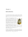


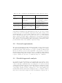


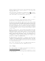


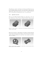

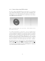


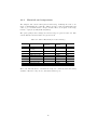


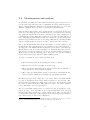


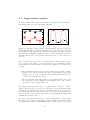


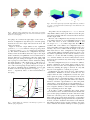


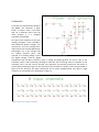


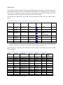
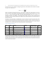


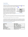
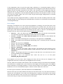
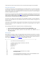
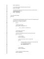

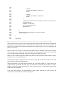


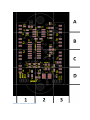

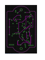
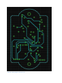


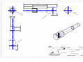


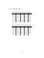


![Documentation technique VS-VSA [4192 ko]](http://vs1.manualzilla.com/store/data/006316293_1-cded0d07eb1da26f2a87274f7f721e39-150x150.png)