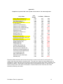
1
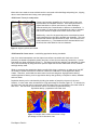
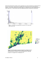
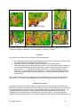
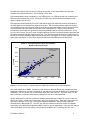
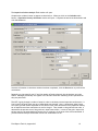
Final Report
Refinement of
Population-Calibrated Land-Cover-Specific
Impervious Surface Coefficients for Connecticut
NEMO FY ’02 Work Plan
DEP Project 01-08
Task #6
Michael (Sandy) Prisloe
Emily Hoffhine Wilson
Chester Arnold
University of Connecticut
Middelsex County Extension Center
1066 Saybrook Road
P.O. Box 70
Haddam, CT 06438-0070
Phone: (860) 345-4511
Fax: (860) 345-3357
Email: [email protected]
Email: [email protected]
Email: [email protected]
Background/previous research
Previous research conducted under 319 funding was performed by Bill Sleavin, a graduate student at
the University of Connecticut, who studied four towns in Connecticut (West Hartford, Marlborough,
Waterford, and Woodbridge). Using highly accurate planimetric GIS data from the four towns, he
developed impervious surface coefficients for Connecticut’s 1995 satellite-derived land cover data.
Using these coefficients it is possible to estimate, based on land cover data, impervious surface
coverage for any Connecticut watershed.
While developing the coefficients Mr. Sleavin observed that, within a single land cover class, a
correlation appeared to exist between the impervious surface coefficient and population density where
the rural town (Marlborough) generally had lower coefficients than the suburban towns (Waterford and
Woodbridge) which had lower coefficients than the urban town (West Hartford). To account for this,
he suggested that three sets of coefficients – one set for rural towns, one set for suburban towns, and
one set for urbanized towns – be developed based on a larger sample of town planimetric datasets.
However, it also was observed that there is significant spatial variability of land use patterns and
densities within a single town and that rural, suburban and urban characterizations based on town
geographies may be too coarse.
Percent Impervious
Prior to the research described herein, the authors had conducted a preliminary investigation into the
relationship between impervious
ALL POINTS BUT ONE OUTLIER
surface and population density. In
this study, the impervious surface
percent area for West Hartford’s
50.0
y = 0.0043x + 10.447
45.0
1990 Census tracts was calculated
R2 = 0.8487
40.0
and plotted against population
35.0
density. A positive correlation
30.0
existed initially and an even
Series1
25.0
stronger correlation was evident
Linear (Series1)
20.0
when one tract was eliminated
15.0
from the analysis (Figure 1). The
10.0
one tract that was eliminated had
5.0
a population density of 2000 and a
0.0
percent impervious of 50% and
0.0
5000.0
10000.0
included a very significant area of
Population Density per Square Mile
“big box” commercial and retail
development.
Figure 1 Percent impervious area for West Hartford Census
tracts plotted against population density.
Based on this and Mr. Sleavin’s
research it was hypothesized that:
(1) there is a correlation between
population density and impervious surface area and (2) this relationship will hold true for impervious
surface coefficients for each of the land cover classes in Connecticut’s 1995 land cover data.
Independent of 319 funding, an Impervious Surface Analysis Tool (ISAT) was developed by the Coastal
Services Center (CSC), National Oceanic and Atmospheric Administration (NOAA), in collaboration with
the NEMO program at the University of Connecticut (Appendix C). The ISAT is an extension for
ArcView3.x (a version for ArcGIS8.x should be ready for distribution in the 4th quarter, 2003) that is
free for download at the CSC website (http://www.csc.noaa.gov/crs/is/). The ISAT can be used to
estimate the percent impervious surface area for any user-selected geographic area. The ISAT requires
a land cover map, a set of impervious surface coefficients calibrated to each land cover class for low,
medium and high population density areas, and an optional population density dataset. The ISAT also
has the ability to model “what if” scenarios where areas of land cover change can be identified and the
impervious surface area is re-calculated to reflect future conditions. The combination of previous
Final Report Task # 6
1
work, the release of the ISAT, and NEMO programmatic needs focused our interest on improving land
cover specific impervious surface coefficients for modeling watershed impervious surface area.
Research Objectives
The principle research goal was to develop a more accurate set of land-cover-specific impervious
surface coefficients, calibrated to low, medium and high population densities, for Connecticut’s 1995
land cover data. To accomplish this, several objectives were defined.
1. The first objective was to increase the sample size used to calculate impervious surface
coefficients. This would require acquiring accurate planimetric GIS data of impervious surface
landscape features – building outlines, driveways, parking lots, etc. – from additional
Connecticut municipalities. A larger sample would result in more accurate coefficients by
increasing the set of land cover classes in the sample and by increasing the geographic area of
each land cover, thereby reducing the effects of outliers or small areas with atypical land use
patterns.
2. The second objective was to refine the methodology and data used to develop the impervious
surface coefficients. Rather than calculating coefficients based on municipal geographies as
previously had been done, our approach was to use 1990 Census tracts as the geographic unit
over which coefficients would be developed. If the amount of impervious surface within a land
cover class is correlated to population density, then it would be desirable to have population
density data uniformly distributed over relatively small geographic areas. By using Census
tracts we could use consistent definitions for low, medium or high population density areas. It
also was a goal to use a quantitative measure rather than a subjective classification such as
rural, suburban and urban.
Methods
Datasets
All datasets used in the project were, if necessary, projected to Connecticut State Plane Coordinates,
NAD83, units feet.
The 1995 Connecticut land cover dataset was developed at the Laboratory for Earth Resource
Information Systems (LERIS) at the University of Connecticut. It was derived predominantly from 1995
satellite imagery. It has a spatial resolution of 100ft (each pixel represents a 100’x100’ square on the
ground). For details about the methodology used to create these data, see Civco and Hurd, 19991.
The census tracts were from the US Census Bureau and represent the 1990 track boundaries. Because
the 1995 land cover data fell half way between the 1990 and 2000 censuses, either set of tract
boundaries could have been used. However, the majority of planimetric data available early in the
study was closer to the 1990 census year leading us to use the 1990 census tracts. Some of the
planimetric data that have been made available more recently are closer to the 2000 census.
Nine Connecticut towns generously provided their planimetric data. The towns are: Groton,
Marlborough, Milford, Stamford, Stonington, Suffield, Waterford, West Hartford, and Woodbridge.
These towns are geographically spread across the state and represent many regions. The authors
recognize that the mix of land cover in the sample towns does not match exactly the statewide
distribution of land (Appendix B). The entire set of sample towns had higher percentages of urban land
covers; however, this was not a concern because most impervious surface area is associated with urban
land covers.
1
http://resac.uconn.edu/publications/tech_papers/pdf_paper/Civco_and_Hurd_ASPRS_1999.pdf
Final Report Task # 6
2
Data Preprocessing Steps
Land Cover Data – Addition of a Shoreline Class
In the previous analyses by Bill Sleavin, impervious surface coefficients
for the deep water class for the four towns were calculated to be 1.27,
0.98, 0.64 and 0.35. In some cases, water can have an impervious
surface coefficient value due to features such as bridges. However,
the calculated coefficients were found to be artificially high due to the
mixed pixel problem inherent with classification of medium resolution
satellite imagery. The mixed pixel problem (Figure 2) occurs when a
pixel in an image (100ft by 100ft) contains more than one feature on
the earth; the pixel could be classified as water but could actually
contain some land with impervious features.
The result is an impervious surface coefficient for the water class that
is artificially inflated and substantially higher than 0. In most areas in
Connecticut, the area of deep water is very small and thus contributes
little to the overall impervious surface estimate. However, in areas
with large bodies of water, a deep water impervious surface coefficient incorrectly contributes
significant amounts of impervious surface area to the estimate. To remedy this problem, a shoreline
class was added to the land cover map and an impervious surface coefficient for shorelines was
calculated. The shoreline class is a one-pixel buffer, created using ERDAS Imagine image processing
software, on the inside of all deep water features (Figure 3).
Figure 2 Mixed-pixels at
the edge of a waterbody.
Figure 3 Part of Candlewood Lake with the original water class (left) and with the
shoreline class in white (right).
Planimetric Impervious Surface Feature Data
The impervious surface data used for the project were extracted from the municipal planimetric
datasets provided by the nine towns that participated in the study. Extracted features included
buildings (building footprints), driveways, roads, parking lots, sidewalks and in some cases tennis
courts, basketball courts, swimming pools and miscellaneous impervious landscape features.
Impervious surface feature data for each town were converted to an ESRI shapefile polygon format.
Final Report Task # 6
3
Minor edits were made to remove islands such as courtyards within buildings and parking lots, clipping
data to town boundaries and closing some open polygons.
1990 Census Tracts for study towns
Census tract boundary shapefiles for the nine study towns were
downloaded from the MAGIC web site. Edits were performed to
adjust boundaries to follow road centers or other landscape
features used by the Census Bureau to define tract boundaries. It
was necessary to adjust the tract boundaries in order to calculate
the correct amount of impervious surface area for each tract.
Additionally, tracts for the nine study towns were edited to match
town boundaries from the DEP’s detailed town shapefile. The Long
Island Sound coastline and shorelines of major rivers that serve as
town boundaries (e. g. The Housatonic River between Milford and
Stratford) also were added to the tract datasets.
Figure 4 Original (yellow) and edited
(purple) Census tract boundaries
1990 Statewide Census tracts – establishing population density thresholds
One of our initial assumptions was that impervious surface area within each land cover class is
positively correlated to population density and that, at least for most areas in Connecticut, it can be
expressed as a linear relationship (Figure 1). The Impervious Surface Analysis Tool (Appendix C) makes
use of this relationship by using land cover specific impervious surface coefficients for low, medium
and high density areas.
While we recognize that population density actually falls along a continuum, to make use of the ISAT
we needed to create three distinct classes of coefficients calibrated to three population density
classes. Therefore, we divided the census tracts into three categories: high population density,
medium population density, and low population density that generally correspond to urban, suburban
and rural areas.
Population density can be calculated by dividing the number of people by the area of the tract.
However, in some cases water accounted for a high percentage of the area (Figure 5). To remedy this,
the land cover map was used in conjunction with the census tracts to calculate the non-water area for
each tract. The non-water area was then used to calculate the population density.
Population density = population/non-water area
Figure 5 Example where coastal tracts have a large
percentage of area in the water class
Final Report Task # 6
4
The divisions between high, medium, and low population tracts were made based on a histogram of the
data and visual analysis. The histogram revealed breaks at 500 people/mi2 and 1800 people/mi2.
(Figure 6). After visual inspection of the state (Figure 7) in conjunction with a priori knowledge about
where people live, it was determined that these population density thresholds were appropriate.
Figure 6 Histogram showing population density for all Connecticut
1990 Census tracts.
Number of
people/mi2
Figure 7 Census tracts for the state of Connecticut divided into three
groups based on population density (utilizing non-water area in the
population density calculation): less than 500 people/mi2, 500-1800
people/mi2, and greater than 1800 people/mi2.
Final Report Task # 6
5
Data Analysis
Impervious Surface Coefficients - Land Cover Specific Coefficients Calibrated to Population Density
After the Census tracts had been classified into high, medium, and low population density tracts, GIS
overlay analyses were conducted to develop land cover specific impervious surface coefficients for
each population density class. Processing of data was done using ArcMap version 8.2. For each town,
the ArcMap geoprocessing wizard was used to union the Census tracts with the 1995 land use land cover
data for the town. The resulting dataset was then unioned with the impervious surface data for the
town. Every polygon in the resulting dataset’s attribute table contained an area value in square feet,
the 1990 tract number, a land use code (1-29), and an impervious surface code (1=impervious, 0=not
impervious). A frequency analysis using the XTOOLS Extension to ArcMap was done to create a
database from which we could determine:
1. the total area of each land cover class within each tract
2. the total area of impervious surface features within each land cover class within each tract
Data were joined with population density classes and were exported from ArcMap to EXCEL. Within
EXCEL, Census tracts falling into each population density class (high, medium, low) were analyzed.
The sum of the impervious surface area for each land cover class was divided by the total area of the
class times 100. This was performed for each land cover class in each population class to develop a full
set of coefficients which are included in Appendix A.
Outliers - Isolate and Analyze Tracts with High Imperviousness and Low-Medium Population Density
There were several cases where the Census tract population density was less than 1800 people/mi2 but
the amount of impervious area was substantial. These cases were generally highly developed
commercial, industrial and/or retail areas or airports with relatively few residents and large impervious
surface areas. These outliers can pose a problem when using the ISAT because, based on population
density, the medium or low population density coefficients would be applied to these tracts, even
though they had impervious surface area more consistent with the high population density coefficients.
Therefore, it was necessary to develop a method by which to identify potential outlier tracts.
This analysis was performed on all 1990 Census tracts. The first step was to determine which tracts
had a high percentage of the 1995 land cover class “Commercial/Industrial/Pavement.” A single factor
dataset that included only the “commercial/industrial/pavement” class was created from the land
cover. A second dataset that included all areas except water was also produced. The area of
“commercial/industrial/pavement” land cover that existed in each Census tract was determined using
the zonal statistics function of ArcView Spatial Analyst.
These data were analyzed in both map and chart form to identify low to medium population density
Census tracts with high imperviousness. The graph (Figure 8) shows population density and the percent
of “commercial/industrial/pavement” land cover in each tract (note – the tracts with very high
population density are not shown in order to see more detail in the lower population density tracts).
The yellow box identifies all the tracts with greater than 1800 people/mi2 that would automatically
have the high population density coefficients applied when using the ISAT to calculate impervious
surface area. The red box encloses the outliers that have high percentages of “commercial/industrial/
pavement” (high imperviousness) but fewer then 1800 people/mi2.
All tracts with low-medium population density and high percentages of commercial/industrial land
cover are shown in Figure 9. Some detailed example areas are shown in Figure 10.
Final Report Task # 6
6
Figure 8 The population density for all census tracts in Connecticut with densities less
than 14,000 people/mi2 and the percent of commercial/industrial/ pavement land
cover. The tracts in the yellow box have greater than 1800 people/mi2 and therefore
the high population density coefficients would be applied. Those tracts in the red box
are considered to be outliers with low or medium population density and high amounts
of imperviousness.
Number of people/mi2
Figure 9 Connecticut census tracts divided into three categories based on population density. Tracts
considered outliers (low or medium population density and high “commercial/industrial/pavement”
land cover) are outlined in cyan.
Final Report Task # 6
7
Waterbury
Bridgeport and Milford
North Haven and Wallingford
Groton
Hartford and Manchester
Windsor Locks
Figure 10 Examples of census tracts with low or medium population density and high percentage of
“commercial/industrial/pavement” land cover depicted in the dark brick color.
Products
This research has resulted in the creation of the following datasets:
1. Set of impervious surface coefficients, designed to be used with Connecticut’s 1995 land cover
data, and calibrated to population density (Appendix A).
2. A modified 1995 land cover dataset to which a shoreline class has been added.
3. 1990 Census tract dataset with an added field named “Coeff_clas” which contains a code used
to determine which impervious surface coefficient to apply to land cover grid cells that fall
within the tract. (1 = low population density coefficient, 2 = medium population density
coefficient, 3 = high population density coefficient). “Outliers” with low-medium population
density and greater than 20% of the area falling in the “commercial/industrial/paved” class
have a code of 3.
Also provided as part of this report (Appendix D) are detailed instructions on how to use these data
with the ISAT. ISAT software and datasets are stored on a CD-ROM also included with this report.
Validation and Testing
The impervious surface coefficients refined through this project and the previously developed set of
coefficients were used to estimate the percent impervious area for 244 watersheds that fell completely
within the boundaries of the nine towns for which we had planimetric impervious feature data. The
watersheds used for this analysis were extracted from DEP basin shapefile which includes local
drainage basins and drainage areas of impoundments and stream reaches. The actual watershed
impervious surface area was determined for each watershed by overlaying the watershed boundaries on
Final Report Task # 6
8
the impervious feature GIS data and calculating the percent of each watershed’s area that was
comprised of impervious features. This served as “truth” data.
The 244 watersheds varied considerably in size ranging from 5 to 4,298 acres and with a mean size of
470 acres and a median size of 324. Actual percent impervious surface area also exhibited a wide
range in values from 0% to 51%.
The Impervious Surface Analysis Tool (ISAT) was used to apply the impervious surface coefficients to
the watersheds to calculate percent impervious surface. The calculated percent impervious surface
was compared to the actual percent impervious surface to assess the degree to which the coefficients
accurately predict percent impervious surface at the watershed level. Figure 11 plots actual vs.
calculated percent impervious surface for the 244 watersheds based on the new coefficients. A line,
fit to the set of points, has an R2 value of 0.8959 indicating a strong correlation between the actual and
calculated watershed percent impervious surface. This means the impervious surface coefficients can
be used to calculate watershed imperviousness with a fairly high degree of accuracy although there are
cases where calculated vs. actual show significant differences (see Discussion section below).
Actual vs. Calculated Percent Impervious Surface
Based on New Coefficients
60.00
y = 0.892x + 1.2563
R2 = 0.8959
50.00
Calculated
40.00
30.00
20.00
10.00
0.00
0.00
10.00
20.00
30.00
40.00
50.00
60.00
Actual
Figure 11 Plot of actual vs. calculate percent impervious surface area for 244 watersheds.
Root mean square error (RMSE), a measure of the difference between actual and calculated percent
impervious surface area, also was calculated for the new and previously developed set of coefficients.
The RMSE is 3.30 for the new set of coefficients and 4.52 for the older set. The lower value, for the
new coefficients, indicates a much better prediction for the set of 244 watersheds.
We also examined how well the coefficients handled watersheds that covered all or part of what we
refer to as “outlier” Census tracts (there were ten in our sample of 244). These are tracts with more
than 20% of the land cover in the “Commercial/Industrial/Pavement” class and with population
densities below 1800 people/mi2. The ISAT with the new coefficients and the Census tract dataset
with outlier tracts identified produced an RMSE of 3.89 for the ten watersheds. Using the ISAT and the
older coefficients without the outlier tracts produced an RMSE of 8.77, indicating that the new
Final Report Task # 6
9
methodology does a much better job calculating percent impervious cover for areas that cover outlier
Census tracts.
Using the new set of coefficients, more than 50% of the 244 sample watersheds were ±2 percent of the
actual measured percent impervious surface.
Discussion
While the impervious surface coefficients can be used to calculate the percent impervious surface area
for any Connecticut watershed, there are several things to be aware of when using this methodology.
Calculations for small watersheds are prone to large errors. This is the result of two things that are
closely related: 1) small errors due to inexact coefficients are magnified when expressed over small
geographic areas, and 2) errors in the land cover classifications similarly are magnified when only small
geographic areas are considered. Although we did not thoroughly analyze percent impervious surface
calculation errors relative to watershed size, it may none-the-less be appropriate to limit the
application of these coefficients to watersheds greater than several hundred acres. Future research
would be necessary to determine a minimum watershed size threshold.
There were several moderate size watersheds that exhibited large differences between actual and
calculated percent impervious surface with the calculated amounts being much greater. Two were
located in Groton. We examined these and discovered that almost the entire area of both is comprised
of the Bluff Point Coastal Reserve as shown on the Department of Environmental Protection’s GIS
property dataset. Thus, the watersheds are almost totally devoid of development and are covered
primarily with deciduous forest land cover. It may be beneficial to identify that portion of any
watershed that includes significant amounts of permanently protected open space and to exclude these
areas when calculating percent impervious surface area. This could be done by adding an open space
category to the land cover dataset that would have an impervious surface coefficient of zero.
However, before adopting this approach, research would be necessary to demonstrate that it improves
the calculated results for more than just the two watersheds in Groton.
Conclusions
It is our opinion that the land-cover-specific impervious surface coefficients, calibrated to 1990 Census
tract population density, when used with the Impervious Surface Analysis Tool, can effectively estimate
the percent impervious surface area of Connecticut watersheds or other user-selected geographic
areas. The results of the calculation should be viewed as a “first cut” measure of watershed
imperviousness resulting from anthropogenic factors. There were differences between calculated and
actual percent impervious surface area in the 244 watersheds tested but any broadly applicable model,
due to inherent limitations with models in general, will produce similarly varying results. Our goal in
this research was to improve upon the set of impervious surface coefficients initially developed with
319 funding support. Testing the new coefficients and methodology against that previously developed
resulted in consistently better estimates of percent impervious surface area.
Final Report Task # 6
10
1
2
3
4
5
6
7
8
9
10
11
12
13
14
15
16
17
18
19
20
21
22
23
24
25
26
27
28
29
Class #
Suburban
37.52
27.72
6.45
14.27
2.61
7.13
NA
11.05
8.16
14.65
NA
20.64
1.01
3.11
0.34
1.00
NA
10.31
0.38
0.45
1.64
2.60
9.20
0.45
3.45
NA
0.36
8.91
NA
Urban
59.34
40.54
10.79
18.24
5.38
9.24
NA
15.23
6.57
18.07
NA
NA
2.83
4.17
0.70
3.81
NA
14.55
28.06
1.27
5.44
21.56
30.58
10.79
37.18
NA
NA
31.57
NA
30.15
22.80
15.28
13.20
4.85
4.54
NA
7.45
2.43
10.43
NA
NA
0.82
2.11
0.01
1.26
NA
0.40
0.36
0.64
2.29
2.30
11.62
0.58
NA
NA
NA
NA
NA
Rural
New Coefficients
High
Medium
Low
Population
Population
Population
Density**
Density**
Density**
55.70
41.76
32.51
38.49
28.69
25.98
12.42
8.11
8.81
17.80
15.08
12.65
4.97
5.75
3.63
10.13
8.83
4.06
0*
3.69
0.31
11.26
9.80
6.60
10.45
6.44
2.09
22.65
9.21
4.53
0*
0*
0.84
0*
23.65
0.92
1.64
1.21
0.95
4.08
3.85
2.34
0.70
1.57
0.30
7.21
2.24
0.97
0.00
0*
0.00
10.05
9.66
10.42
19.70
1.59
0.71
0.76
0.08
0.10
9.85
3.95
1.92
15.34
5.38
2.57
29.83
4.89
4.84
17.90
0.89
0.63
35.71
1.14
1.31
1.35
0.70
3.18
4.05
2.51
5.52
23.56
12.27
10.47
3.83
1.51
1.51
Appendix A: Impervious Surface Coefficients
Original Coefficients
3.64
2.05
(1.63)
0.44
0.41
(0.89)
NA
3.97
(3.88)
(4.58)
NA
NA
1.19
0.09
0.00
(3.40)
NA
4.50
8.36
0.51
(4.41)
6.22
0.75
(7.11)
1.47
NA
NA
8.01
NA
Final Report Task # 6, Appendix A
11
(4.24)
(0.97)
(1.66)
(0.81)
(3.14)
(1.70)
NA
1.25
1.72
5.44
NA
(3.01)
(0.20)
(0.74)
(1.23)
(1.24)
NA
0.65
(1.21)
0.37
(2.31)
(2.78)
4.31
(0.44)
2.31
NA
(2.15)
(3.36)
NA
(2.36)
(3.18)
6.47
0.55
1.22
0.48
NA
0.85
0.34
5.90
NA
NA
(0.13)
(0.23)
(0.29)
0.29
NA
(10.02)
(0.35)
0.54
0.37
(0.27)
6.78
(0.05)
NA
NA
NA
NA
NA
Difference (Original – New)
* No area of this class was present in any of the samples.
** Populations densities are: High > 1,800 people/mi2, 1,800 people/mi2 > Medium > 500 people/mi2, Low < 500 people/mi2
Commercial/Industrial/Pavement
Residential/Commercial
Rural Residential
Turf & Tree Complex
Turf & Grass
Pasture & Hay & Grass
Pasture & Hay / Cropland
Pasture & Hay / Exposed Soil
Exposed Soil / Cropland
Exposed Soil
Shade-grown Tobacco
Nursery Stock
Scrub & Shrub
Deciduous Forest
Deciduous Forest & Mt. Laurel
Coniferous Forest
Dead & Dying Hemlock
Forest / Clear Cut
Mixed Forest
Deep Water
Shallow Water & Mud Flats
Non-forested Wetland
Deciduous Shrub Wetland
Deciduous Forested Wetland
Coniferous Forested Wetland
Low Coastal Marsh
High Coastal Marsh
Exposed Ground & Sand
Shoreline
Land Cover Class Name
Land Cover
New Impervious Surface Coefficients and Percentage of Land Cover
Land Cover
Land Cover Class
Class
Commercial/Industrial/Pavement
Residential/Commercial
Rural Residential
Turf & Tree Complex
Turf & Grass
Pasture & Hay & Grass
Pasture & Hay / Cropland
Pasture & Hay / Exposed Soil
Exposed Soil / Cropland
Exposed Soil
Shade-grown Tobacco
Nursery Stock
Scrub & Shrub
Deciduous Forest
Deciduous Forest & Mt. Laurel
Coniferous Forest
Dead & Dying Hemlock
Forest / Clear Cut
Mixed Forest
Deep Water
Shallow Water & Mud Flats
Non-forested Wetland
Deciduous Shrub Wetland
Deciduous Forested Wetland
Coniferous Forested Wetland
Low Coastal Marsh
High Coastal Marsh
Exposed Ground & Sand
Shoreline
1
2
3
4
5
6
7
8
9
10
11
12
13
14
15
16
17
18
19
20
21
22
23
24
25
26
27
28
29
New Coefficients
High
Medium
Low
Population
Population Population
Density
Density
Density
55.70
41.76
32.51
38.49
28.69
25.98
12.42
8.11
8.81
17.80
15.08
12.65
4.97
5.75
3.63
10.13
8.83
4.06
0*
3.69
0.31
11.26
9.80
6.60
10.45
6.44
2.09
22.65
9.21
4.53
0*
0*
0.84
0*
23.65
0.92
1.64
1.21
0.95
4.08
3.85
2.34
0.70
1.57
0.30
7.21
2.24
0.97
0.00
0*
0.00
10.05
9.66
10.42
19.70
1.59
0.71
0.76
0.08
0.10
9.85
3.95
1.92
15.34
5.38
2.57
29.83
4.89
4.84
17.90
0.89
0.63
35.71
1.14
1.31
1.35
0.70
3.18
4.05
2.51
5.52
23.56
12.27
10.47
3.83
1.51
1.51
% of IS Contribution
High
Medium
Low
Population Population Population
Density
Density
Density
43.59
27.60
19.95
41.95
32.93
18.67
0.35
2.15
3.31
9.21
13.03
11.54
0.77
1.40
0.73
0.51
3.98
11.37
0.00
0.00
0.01
0.36
0.70
0.70
0.16
0.36
1.18
0.17
0.43
1.58
0.00
0.00
0.02
0.00
0.01
0.01
0.00
0.05
0.22
0.74
14.42
27.48
0.00
0.04
0.05
0.22
0.81
1.38
0.00
0.00
0.00
0.06
0.12
0.03
0.03
0.06
0.06
0.00
0.01
0.01
0.08
0.16
0.08
0.15
0.21
0.24
0.08
0.18
0.26
0.03
0.04
0.09
0.01
0.03
0.12
0.09
0.03
0.04
0.20
0.24
0.37
1.17
0.82
0.32
0.06
0.19
0.18
This table lists the new land cover impervious surface coefficients for each of the twenty-nine land
cover classes for each population density class. The table also includes data on the percent of total
impervious surface within each population density class that is derived from each land cover type. It is
important to understand this relationship. For example: 55.7% of the area of the land cover class
“Commercial/Industrial/Pavement” is covered with impervious surface features in the high population
density tracts that were studied and this land cover class accounted for 43.59% of all impervious
surface within the high population density tracts. Compare this to the land cover class “Deciduous
Forested Wetland” that also has a relatively high impervious surface coefficient of 35.71% but that
accounts for ONLY 0.01% of total impervious surface area within the high population density tracts.
Those land cover classes we have judged to be significant contributors to overall impervious area (i. e.
they account for at least 1% of total impervious area within a population density class) are highlighted
in cyan. It is interesting to note that the highlighted land cover classes account for nearly all of the
impervious surface area (95.92% for the high population density tracts, 95.51% for the medium
population density tracts, and 93.73% for the low population density tracts).
Final Report Task # 6, Appendix A
12
Appendix B:
Comparison of percent land cover by class for the state vs. the nine study towns
LULC Class
Comm./Indust./Pavement (1)
Residential/Commercial (2)
Rural Residential (3)
Turf & Tree Complex (4)
Turf & Grass (5)
Pasture & Hay & Grass (6)
Pasture & Hay / Cropland (7)
Pasture & Hay / Exposed Soil (8)
Exposed Soil / Cropland (9)
Exposed Soil (10)
Shadegrown Tobacco (11)
Nursery Stock (12)
Scrub & Shrub (13)
Deciduous Forest (14)
Deciduous Forest & Mt. Laurel (15)
Coniferous Forest (16)
Dead & Dying Hemlock (17)
Forest / Clear Cut (18)
Mixed Forest (19)
Deep Water (20)
Shallow Water & Mud (21)
Non-forested Wetland (22)
Deciduous Shrub Wetland (23)
Deciduous Forested Wetland (24)
Coniferous Forested Wetland (25)
Low Coastal Marsh (26)
High Coastal Marsh (27)
Exposed Ground & Sand (28)
Shoreline (29)
% of
Sample
8.29
11.96
2.08
8.25
2.25
8.49
0.07
0.70
1.59
1.02
0.06
0.03
0.70
42.93
0.53
4.90
0.00
0.09
0.36
1.27
0.33
0.42
0.28
0.53
0.31
0.32
0.65
0.57
0.98
% of State
Difference
4.37
6.50
1.63
4.87
1.59
8.59
0.02
0.73
1.79
0.96
0.03
0.04
0.62
50.21
1.42
10.18
0.01
0.09
0.97
1.58
0.51
0.57
0.28
0.41
0.30
0.14
0.24
0.33
0.99
3.92
5.46
0.45
3.38
0.66
(0.10)
0.05
(0.03)
(0.20)
0.06
0.03
(0.01)
0.08
(7.28)
(0.89)
(5.28)
(0.01)
0.00
(0.61)
(0.31)
(0.18)
(0.15)
0.00
0.12
0.01
0.18
0.41
0.24
(0.01)
The above table summarizes and contrasts the percent of total area for each of the 29 land cover
classes within the state and the nine study towns. The land cover classes with large differences are
highlighted in yellow and reflect the fact that the towns used in the study were more “urbanized” than
the state as a whole. The increase in urban land covers in the sample set (class 1, 2 and 4) vs. the
state as a whole was 12.76% while the decrease in forested classes (class 14 and 16) was 12.56% essentially offsetting one another.
Final Report Task # 6, Appendix B
13
Appendix C:
The Impervious Surface Analysis Tool (ISAT)
Determining the Percentage of
Impervious Surface in a Region
The Impervious Surface Analysis Tool (ISAT), an ArcView 3.x extension, is used to calculate the
percentage of impervious surface area of user selected geographic areas (e.g. watersheds,
municipalities, subdivisions). The National Oceanic and Atmospheric Administration (NOAA) Coastal
Services Center and the University of Connecticut’s Nonpoint Education for Municipal Officials
(NEMO) Program developed this tool for coastal and natural resource managers.
Why Quantify Impervious Surfaces?
In a watershed, the correlation between
impervious surfaces and water quality has been
well established, but determining the amount of
impervious surface area can be a difficult and
time consuming process. ISAT was developed
to help managers and planners calculate the
area of impervious surfaces and relate this to
impacts on local water quality.
For more information on:
ISAT
David Eslinger
NOAA Coastal Services Center
2234 South Hobson Avenue
Charleston, South Carolina 29405-2413
E-mail: [email protected]
Impervious Surface Measurement
Sandy Prisloe
University of Connecticut NEMO
Geospatial Technology Program
1066 Saybrook Road
Haddam, Connecticut 06438-0070
E-mail: [email protected]
The Impervious Surface Analysis Tool
• Requires the Spatial Analyst® extension
• Requires the following inputs:
9Land cover grid
9Polygon data set for which percentage of
impervious surface is to be calculated
9Set of land cover impervious surface
coefficients calculated for low, medium, and
high population densities
9Optional population density theme
• Creates the following outputs:
9Shapefile that includes green, yellow, and
red polygons to represent conditions of
good, fair, and poor water quality
9Attribute table that includes a calculated
value for the percent impervious area and
total impervious surface area of each
selected polygon
• Incorporates land cover change scenarios to
examine how changes influence impervious
surfaces
Download ISAT
www.csc.noaa.gov/crs/is
Final Report Task # 6, Appendix C
14
Appendix D
Recommended Procedure for Applying Coefficients to
Connecticut Land Cover Data Using the
Impervious Surface Analysis Tool (ISAT)
The Impervious Surface Analysis Tool, an extension to ArcView 3.x, can be used to apply easily and
quickly the impervious surface coefficients developed through this research to calculate the percent
impervious surface area for watersheds or other user-selected geographic areas. A CD-ROM is provided
that contains the software and data needed to install and use the ISAT.
ISAT requirements:
To use the ISAT, you MUST have a licensed version of ESRI’s ArcView 3.x and ESRI’s Spatial Analyst
Extension must be installed. The ISAT will not work without Spatial Analyst.
CD-ROM contents by folder (note: all the folders are located in the parent folder named DEP-ISAT)
Folder
DEP-ISAT
DEP-ISAT\Grids
DEP-ISAT\IS Coefficients
DEP-ISAT\ISAT Software
DEP-ISAT\Shapes
Contents
lulc.avl
basic_isat.apr
1995_lulc_grd
New_CT_LULC.txt
ISAT.zip
msxml3.exe
Basins
Coeff_class
Description
an ArcView legend file for the land cover grid
an ArcView Project setup for running the ISAT
29-class land cover grid dataset
IS coefficients to be imported into ISAT
ISAT installation files, tutorial data, user manual
system file that may be necessary to install to run ISAT
DEP basin shapefile
1990 Census tracts shapefile used to determine
population densities for ISAT
Copy the folder named DEP-ISAT from the distribution CD-ROM to the C: drive on your PC. When the
folder is copied from the CD, it and all subfolders and files are set to read-only. You will need to reset
the read-only attributes to read-write. With Windows 2000 and Windows XP this is easy and straight
forward. Right click on the C:\DEP-ISAT folder and select Properties. A window will open that looks
like the following. Click on the Attributes: Read-only box and remove the check mark that appears
there. Then Click OK. Another window named Confirm Attribute Changes will appear. Click the
radio button next to Apply changes to this folder, subfolders and files and then click OK.
With Windows NT, 95 and 98 you will need to select
each folder, select its properties and reset the readonly attribute. You’ll also need to select all files
within each folder and go through the same process.
Final Report Task # 6, Appendix D
15
Instructions for installing ISAT:
The file named ISAT.zip contains setup.exe, msxml3.exe (Microsoft® XML Parser), and the files
required to complete a set of ISAT tutorials. To install ISAT, create a c:/isat folder and extract
the zipped files into it. Run the setup.exe program by double-clicking on it. The installation process
will place a copy of the ISAT extension in the ArcView extensions folder, typically located at
C:\Esri\AV_GIS30\Arcview\Ext32. Once the
installation has completed, you can load and
use the ISAT extension by starting ArcView and
selecting Extensions from the file menu. The
ISAT extension will be listed along with the
other extensions. Click the box next to its
name and click OK. The ISAT will be installed
and the Spatial Analyst extension automatically
will be loaded.
After loading ISAT, a new menu choice named
“impervious Surface Tools” will appear on the
View document’s menubar.
Getting started:
There is a project named basic_isat.apr located in the DEP-ISAT folder. Open ArcView 3.x and open
this project. A “default” ISAT project will open that contains the themes you will need to run the ISAT
to calculate watershed percent impervious surface area.
IMPORTANT NOTE: If you
receive an error message
reading “429 can’t create
activeX component” at any
point when running ISAT,
you may need to install
Microsoft® XML Parser on
your system. To install the
Microsoft® XML Parser, run
msxml3.exe by doubleclicking on it. The
msxml3.exe file is included
on the CD or you can
download it from
Microsoft’s web site.
Final Report Task # 6, Appendix D
16
The next thing you will need to do is load the impervious surface coefficients for Connecticut. Click on
the Impervious Surface Tools drop-down menu and select the Change Coefficients… menu choice.
This will open the Change Coefficients window. Click the Import button and
navigate to the file named C:\DEP-ISAT\IS Coefficients\New_CT_LULC.txt as shown in the window
below.
Final Report Task # 6, Appendix D
17
Click on the Open button. You will then be asked to name the new Coefficient Set. Name it
CT_1995_LULC as shown below and click the OK button.
Then Click the QUIT button on the Change Coefficients window to close it. You are now ready to run
the ISAT using coefficients for Connecticut’s 1995 land use land cover data. Note: You only have to
import the impervious surface coefficients once. When you import coefficients, a file that stores
information about them is updated. The next time you run the ISAT extension, all the previously used
coefficient sets will be available.
Calculating Percent Impervious Surface Area for Watersheds:
IMPORTANT NOTE: The ISAT will calculate percent impervious surface area for an entire theme or for
selected polygon features within the theme. If you are going to calculate watershed percent
impervious surface area, be sure to select a subset of watersheds or be prepared to wait a long time
for processing to finish.
Select one or more watersheds from the basin theme for which you want to calculate the percent
impervious surface area. Use the ArcView Select Features tool, run a Query or use any other
technique to select your subset of watersheds.
Click the Impervious Surface Tools drop-down menu and select the Run Impervious Surface Analysis…
Final Report Task # 6, Appendix D
18
The Impervious Surface Analysis Tool window will open.
Complete the window’s boxes to appear as shown below. When you click on the Calculate radio
button, a Population Density Calculation window will open.. Complete the entries as shown below and
click the OK button.
Once the information in the above windows has been completed, click the Run button to perform the
calculations.
Depending on the speed of your PC and the number of basins selected, the calculations may take
awhile. Messages periodically will appear in the ArcView status bar indicating various operations as
they are performed.
The ISAT is going through a number of steps in order to calculate percent impervious surface area. It
first finds all the grids within the set of watersheds you selected. Next, it determines what Census
tract each grid falls within and based on the value of coeff-class determines which population density
set of impervious surface coefficients to use for the grid. Then, based on the grids land use code, it
determines the percent area of the grid that is impervious surface. It sums all the grids’ impervious
surface area for the watershed and converts this to a percent of the area of the entire watershed. If
you had selected multiple watersheds it does this simultaneous for all.
Final Report Task # 6, Appendix D
19
When the ISAT completes its computations, a new theme will be added to the View. It will contain
watersheds, color coded based on the calculated percent impervious surface area (green < 10%, 10% <
yellow < 25%, red > 25%). If you use the ArcView Identify tool and click on a watershed, you will see
the attributes that ISAT has created for the new theme (see below).
Four values are calculated as a result of running the ISAT. These are:
TotalAcres
TotalISAcres
pctIS
Complete
– total area of the watershed in acres
- the sum of calculated impervious surface area
- the percent of the watershed that is impervious surface
- Y or N; Y means the land cover was available for the entire watershed
N means that there was incomplete coverage of land cover data
To run the ISAT again, simply select the set of watersheds that you want calculations performed on and
then repeat the steps described above beginning at “Calculating Percent Impervious Surface Area for
Watersheds.”
Other Considerations:
The ISAT includes the capability of modeling percent impervious surface change from hypothetical land
use change. To learn how to use this “what-if” functionality, read the Users’ Manual
(ISAT_Tutorial_v202.pdf) that is included in the ISAT.zip file. The Users’ Manual also includes a
tutorial, but not with Connecticut data, and useful information on troubleshooting typical problems
that people have encountered when working with the ISAT.
There also is a very useful online Help function that is accessed by clicking on the Impervious Surface
Tools and selecting Help from the drop down menu.
Final Report Task # 6, Appendix D
20