Download SECTION 2-6 Inverse Functions

182
2 Graphs and Functions
SECTION
2-6
Inverse Functions
• One-to-One Functions
• Inverse Functions
Many important mathematical relationships can be expressed in terms of functions.
For example,
C d f(d)
The circumference of a circle is a function of the diameter d.
V s g(s)
The volume of a cube is a function of the edge s.
d 1,000 100p h(p)
The demand for a product is a function of the price p.
9
F C 32
5
Temperature measured in °F is a function of temperature in °C.
3
In many cases, we are interested in reversing the correspondence determined by a
function. Thus,
d
C
m(C)
3
s
V n(V)
p 10 1
d r(d)
100
5
C (F 32)
9
The diameter of a circle is a function of the circumference C.
The edge of a cube is a function of the volume V.
The price of a product is a function of the demand d.
Temperature measured in °C is a function of temperature in °F.
As these examples illustrate, reversing the relationship between two quantities often
produces a new function. This new function is called the inverse of the original function. Later in this text we will see that many important functions (for example, logarithmic functions) are actually defined as the inverses of other functions.
In this section, we develop techniques for determining whether the inverse function exists, some general properties of inverse functions, and methods for finding the
rule of correspondence that defines the inverse function. A review of Section 2-3 will
prove very helpful at this point.
• One-to-One
Recall the set form of the definition of a function:
Functions
A function is a set of ordered pairs with the property that no two ordered
pairs have the same first component and different second components.
However, it is possible that two ordered pairs in a function could have the same second component and different first components. If this does not happen, then we call
the function a one-to-one function. It turns out that one-to-one functions are the only
functions that have inverse functions.
2-6
DEFINITION 1
183
Inverse Functions
One-to-One Function
A function is one-to-one if no two ordered pairs in the function have the same
second component and different first components.
To illustrate this concept, consider the following three sets of ordered pairs:
f {(0, 3), (0, 5), (4, 7)}
g {(0, 3), (2, 3), (4, 7)}
h {(0, 3), (2, 5), (4, 7)}
Set f is not a function because the ordered pairs (0, 3) and (0, 5) have the same first
component and different second components. Set g is a function, but it is not a oneto-one function because the ordered pairs (0, 3) and (2, 3) have the same second component and different first components. But set h is a function, and it is one-to-one.
Representing these three sets of ordered pairs as rules of correspondence provides
some additional insight into this concept.
f
Domain
Domain
3
0
0
4
f is not a function.
EXAMPLE 1
h
g
Range
Range
Domain
Range
0
3
2
5
4
7
3
5
2
7
4
7
g is a function but is not
one-to-one.
h is a one-to-one
function.
Determining Whether a Function Is One-to-One
Determine whether f is a one-to-one function for:
(A) f(x) x2
Solutions
(B) f (x) 2x 1
(A) To show that a function is not one-to-one, all we have to do is find two different ordered pairs in the function with the same second component and different
first components. Since
f (2) 22 4
and
f (2) (2)2 4
the ordered pairs (2, 4) and (2, 4) both belong to f and f is not one-to-one.
(B) To show that a function is one-to-one, we have to show that no two ordered pairs
have the same second component and different first components. To do this, we
assume there are two ordered pairs (a, f (a)) and (b, f(b)) in f with the same second components and then show that the first components must also be the same.
That is, we show that f (a) f(b) implies a b. We proceed as follows:
184
2 Graphs and Functions
f(a) f(b)
2a 1 2b 1
2a 2b
ab
Assume second components are equal.
Evaluate f (a) and f(b).
Simplify.
Conclusion: f is one-to-one
Thus, by Definition 1, f is a one-to-one function.
Matched Problem 1
Determine whether f is a one-to-one function for:
(A) f (x) 4 x2
(B) f (x) 4 2x
The methods used in the solution of Example 1 can be stated as a theorem.
Theorem 1
One-to-One Functions
1. If f (a) f(b) for at least one pair of domain values a and b, a b, then f
is not one-to-one.
2. If the assumption f(a) f (b) always implies that the domain values a and
b are equal, then f is one-to-one.
Applying Theorem 1 is not always easy—try testing f(x) x3 2x 3, for
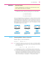
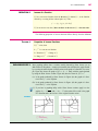
example. However, if we are given the graph of a function, then there is a simple
graphic procedure for determining if the function is one-to-one. If a horizontal line
intersects the graph of a function in more than one point, then the function is not oneto-one, as shown in Figure 1(a). However, if each horizontal line intersects the graph
in one point, or not at all, then the function is one-to-one, as shown in Figure 1(b).
These observations form the basis for the horizontal line test.
FIGURE 1 Intersections of graphs
and horizontal lines.
y
y
y f (x)
(a, f (a))
(b, f (b))
(a, f (a))
y f (x)
a
b
f (a) f(b) for a b
f is not one-to-one
(a)
x
a
Only one point has ordinate
f (a); f is one-to-one
(b)
x
2-6
Theorem 2
Inverse Functions
185
Horizontal Line Test
A function is one-to-one if and only if each horizontal line intersects the graph
of the function in at most one point.
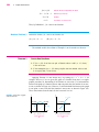
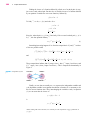
The graphs of the functions considered in Example 1 are shown in Figure 2.
Applying the horizontal line test to each graph confirms the results we obtained in
Example 1.
y
FIGURE 2 Applying the horizontal
line test.
y
5
5
(2, 4)
(2, 4)
5
5
5
x
5
x
5
f(x) x does not pass
the horizontal line test;
f is not one-to-one
(a)
f (x) 2x 1 passes
the horizontal line test;
f is one-to-one
(b)
2
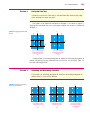
A function that is increasing throughout its domain or decreasing throughout its
domain will always pass the horizontal line test [see Figs. 3(a) and 3(b)]. Thus, we
have the following theorem.
Theorem 3
Increasing and Decreasing Functions
If a function f is increasing throughout its domain or decreasing throughout its
domain, then f is a one-to-one function.
FIGURE 3 Increasing, decreasing,
and one-to-one functions.
y
y
x
y
x
An increasing function
is always one-to-one
A decreasing function
is always one-to-one
(a)
(b)
x
A one-to-one function
is not always increasing
or decreasing
(c)
186
2 Graphs and Functions
The converse of Theorem 3 is false. To see this, consider the function graphed
in Figure 3(c). This function is increasing on (, 0] and decreasing on (0, ), yet
the graph passes the horizontal line test. Thus, this is a one-to-one function that is
neither an increasing function nor a decreasing function.
• Inverse Functions
Now we want to see how we can form a new function by reversing the correspondence determined by a given function. Let g be the function defined as follows:
g {(3, 9), (0, 0), (3, 9)}
g is not one-to-one.
Notice that g is not one-to-one because the domain elements 3 and 3 both correspond to the range element 9. We can reverse the correspondence determined by function g simply by reversing the components in each ordered pair in g, producing the
following set:
G {(9, 3), (0, 0), (9, 3)}
G is not a function.
But the result is not a function because the domain element 9 corresponds to two different range elements, 3 and 3. On the other hand, if we reverse the ordered pairs
in the function
f {(1, 2), (2, 4), (3, 9)}
f is one-to-one.
F {(2, 1), (4, 2), (9, 3)}
F is a function.
we obtain
This time f is a one-to-one function, and the set F turns out to be a function also.
This new function F, formed by reversing all the ordered pairs in f, is called the
inverse of f and is usually denoted* by f 1. Thus,
f 1 {(2, 1), (4, 2), (9, 3)}
The inverse of f
Notice that f 1 is also a one-to-one function and that the following relationships
hold:
Domain of f 1 {2, 4, 9} Range of f
Range of f 1 {1, 2, 3} Domain of f
Thus, reversing all the ordered pairs in a one-to-one function forms a new one-to-one
function and reverses the domain and range in the process. We are now ready to present a formal definition of the inverse of a function.
*f 1, read “f inverse,” is a special symbol used here to represent the inverse of the function f. It does
not mean 1/f.
2-6
DEFINITION 2
Inverse Functions
187
Inverse of a Function
If f is a one-to-one function, then the inverse of f, denoted f 1, is the function
formed by reversing all the ordered pairs in f. Thus,
f 1 {(y, x) (x, y) is in f }
If f is not one-to-one, then f does not have an inverse and f 1 does not exist.
The following properties of inverse functions follow directly from the definition.
Theorem 4
Properties of Inverse Functions
If f 1 exists, then
1. f 1 is a one-to-one function.
2. Domain of f 1 Range of f
3. Range of f 1 Domain of f
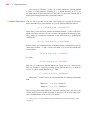
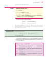
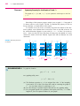
EXPLORE-DISCUSS 1
Most graphing utilities have a routine, usually denoted by Draw Inverse (or an
abbreviation of this phrase—consult your manual), that will draw the graph formed
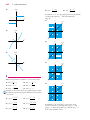
by reversing the ordered pairs of all the points on the graph of a function. For example, Figure 4(a) shows the graph of f(x) 2x 1 along with the graph obtained
by using the Draw Inverse routine. Figure 4(b) does the same for f(x) x2.
(A) Is the graph produced by Draw Inverse in Figure 4(a) the graph of a function? Does f 1 exist? Explain.
(B) Is the graph produced by Draw Inverse in Figure 4(b) the graph of a function? Does f 1 exist? Explain.
(C) If you have a graphing utility with a Draw Inverse routine, apply it to the
graphs of y x 1 and y 4x x2 to determine if the result is the graph
of a function and if the inverse of the original function exists.
FIGURE 4
3
y1
3
y2
3
3
3
y1 2x 1
y2 Draw Inverse y1
(a)
y1
3
y2
3
3
y1 x 2
y2 Draw Inverse y1
(b)
188
2 Graphs and Functions
Finding the inverse of a function defined by a finite set of ordered pairs is easy;
just reverse each ordered pair. But how do we find the inverse of a function defined
by an equation? Consider the one-to-one function f defined by
f(x) 2x 1
To find f 1, we let y f (x) and solve for x:
y 2x 1
y 1 2x
1
2y
12 x
Since the ordered pair (x, y) is in f if and only if the reversed ordered pair (y, x) is
in f 1, this last equation defines f 1:
x f 1(y) 12 y 12
(1)
Something interesting happens if we form the composition* of f and f 1 in either
of the two possible orders
f 1[ f(x)] f 1[2x 1] 12(2x 1) 12 x 12 12 x
and
f[ f 1(y)] f(12 y 12) 2(12 y 12) 1 y 1 1 y
These compositions indicate that if f maps x into y, then f 1 maps y back into x and
if f 1 maps y into x, then f maps x back into y. This is interpreted schematically in
Figure 5.
FIGURE 5 Composition of f and
f 1.
DOMAIN f
RANGE f
f
f (x)
x
f
1(y)
RANGE f 1
y
f 1
DOMAIN f 1
Finally, we note that we usually use x to represent the independent variable and
y the dependent variable in an equation that defines a function. It is customary to do
this for inverse functions also. Thus, interchanging the variables x and y in equation
(1), we can state that the inverse of
y f(x) 2x 1
is
y f 1(x) 12 x 12
*When working with inverse functions, it is customary to write compositions as f [g(x)] rather than as
( f g)(x).
2-6
Inverse Functions
189
In general, we have the following result:
Theorem 5
Relationship between f and f 1
If f 1 exists, then
1. x f 1(y) if and only if y f(x).
2. f 1[ f(x)] x for all x in the domain of f.
3. f [ f 1(y)] y for all y in the domain of f 1 or, if x and y have been interchanged, f [ f 1(x)] x for all x in the domain of f 1.
If f and g are one-to-one functions satisfying
f [g(x)] x
for all x in the domain of g
g[ f(x)] x
for all x in the domain of f
then it can be shown that g f 1 and f g1. Thus, the inverse function is the only
function that satisfies both these compositions. We can use this fact to check that we
have found the inverse correctly.
EXPLORE-DISCUSS 2
Find f [g(x)] and g[ f(x)] for
f (x) (x 1)3 2
and
g(x) (x 2)1/3 1
How are f and g related?
The procedure for finding the inverse of a function defined by an equation is
given in the next box. This procedure can be applied whenever it is possible to solve
y f(x) for x in terms of y.
Finding the Inverse of a Function f
Step 1. Find the domain of f and verify that f is one-to-one. If f is not one-toone, then stop, since f 1 does not exist.
Step 2. Solve the equation y f(x) for x. The result is an equation of the form
x f 1(y).
Step 3. Interchange x and y in the equation found in step 2. This expresses f 1
as a function of x.
Step 4. Find the domain of f 1. Remember, the domain of f 1 must be the
same as the range of f.
190
2 Graphs and Functions
Check your work by verifying that
f 1[ f (x)] x
for all x in the domain of f
and
f [ f 1(x)] x
EXAMPLE 2
for all x in the domain of f 1
Finding the Inverse of a Function
Find f 1 for f(x) x 1
Solution
y
Step 1. Find the domain of f and verify that f is one-to-one. The domain of f is
[1, ). The graph of f in Figure 6 shows that f is one-to-one, hence f 1 exists.
Step 2. Solve the equation y f (x) for x.
5
y f(x)
5
y x 1
y2 x 1
x
x y2 1
5
Thus,
f(x) x 1, x 1
FIGURE 6
x f 1(y) y2 1
Step 3. Interchange x and y.
y f 1(x) x2 1
Step 4. Find the domain of f 1. The equation f 1(x) x2 1 is defined for all values of x, but this does not tell us what the domain of f 1 is. Remember, the
domain of f 1 must equal the range of f. From the graph of f, we see that
the range of f is [0, ). Thus, the domain of f 1 is also [0, ). That is,
f 1(x) x2 1
Check
x0
For x in [1, ), the domain of f, we have
f 1[ f(x)] f 1(x 1)
(x 1)2 1
x11
⁄x
2-6
191
Inverse Functions
For x in [0, ), the domain of f 1, we have
f [ f 1(x)] f(x 2 1)
(x 2 1) 1
x 2
x
x 2 x for any real number x .
⁄x
x x for x 0.
Find f 1 for f(x) x 2.
Matched Problem 2
EXPLORE-DISCUSS 3
Most basic arithmetic operations can be reversed by performing a second operation: subtraction reverses addition, division reverses multiplication, squaring
reverses taking the square root, etc. Viewing a function as a sequence of reversible
operations gives additional insight into the inverse function concept. For example,
the function f(x) 2x 1 can be described verbally as a function that multiplies
each domain element by 2 and then subtracts 1. Reversing this sequence describes
a function g that adds 1 to each domain element and then divides by 2, or
g(x) (x 1)/2, which is the inverse of the function f. For each of the following functions, write a verbal description of the function, reverse your description,
and write the resulting algebraic equation. Verify that the result is the inverse of
the original function.
(A) f(x) 3x 5
(B) f(x) x 1
(C) f(x) 1
x1
There is an important relationship between the graph of any function and its
inverse that is based on the following observation: In a rectangular coordinate system, the points (a, b) and (b, a) are symmetric with respect to the line y x
[see Fig. 7(a)]. Theorem 6 is an immediate consequence of this observation.
FIGURE 7 Symmetry
with respect to the line
y x.
y
5
y
yx
(1, 4)
y f (x)
y
yx
5
y
f 1(x)
y f 1(x)
yx
10
(3, 2)
(4, 1)
x
5
5
5
5
x
y f(x)
(5, 2)
(2, 3)
5
(2, 5)
(a, b) and (b, a)
are symmetric with
respect to the line y x
(a)
5
10
f (x) 2x 1
f 1(x) 12 x 12
f (x) x 1
f 1(x) x 2 1, x 0
(b)
(c)
x
192
2 Graphs and Functions
Symmetry Property for the Graphs of f and f 1
Theorem 6
The graphs of y f(x) and y f 1(x) are symmetric with respect to the line
y x.
Knowledge of this symmetry property makes it easy to graph f 1 if the graph of
f is known, and vice versa. Figures 7(b) and 7(c) illustrate this property for the two
inverse functions we found earlier in this section.
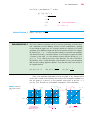
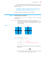
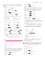
If a function is not one-to-one, we usually can restrict the domain of the function to produce a new function that is one-to-one. Then we can find an inverse for
the restricted function. Suppose we start with f (x) x2 4. Since f is not one-toone, f 1 does not exist [Fig. 8(a)]. But there are many ways the domain of f can be
restricted to obtain a one-to-one function. Figures 8(b) and 8(c) illustrate two such
restrictions.
FIGURE 8 Restricting the domain
of a function.
y
y
y f (x)
5
yx
y
y h(x)
5
yx
5
y g1(x)
5
5
x
5
f (x) x 2 4
f 1 does not exist
(a)
EXPLORE-DISCUSS 4
5
5
5
x
5
y g(x)
5
5
g(x) x 2 4, x 0
g1(x) x 4, x 4
(b)
x
y h 1(x)
h(x) x 2 4, x 0
h1(x) x 4, x 4
(c)
To graph the function
g(x) x2 4,
x0
on a graphing utility, enter
y1 (x2 4)/(x 0)
(A) The Boolean expression (x 0) is assigned the value 1 if the inequality
is true and 0 if it is false. How does this result in restricting the graph of
x2 4 to just those values of x satisfying x 0?
(B) Use this concept to reproduce Figures 8(b) and 8(c) on a graphing utility.
(C) Do your graphs appear to be symmetric with respect to the line y x? What
happens if you use a squared window for your graph?
2-6
Inverse Functions
193
Recall from Theorem 2 that increasing and decreasing functions are always oneto-one. This provides the basis for a convenient and popular method of restricting the
domain of a function:
If the domain of a function f is restricted to an interval on the x axis
over which f is increasing (or decreasing), then the new function determined by this restriction is one-to-one and has an inverse.
We used this method to form the functions g and h in Figure 8.
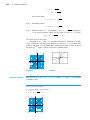
EXAMPLE 3
Finding the Inverse of a Function
Find the inverse of f(x) 4x x2, x 2. Graph f, f 1, and y x in the same
coordinate system.
Solution
Step 1. Find the domain of f and verify that f is one-to-one. The graph of y 4x x2
is the parabola shown in Figure 9(a). Restricting the domain of f to x 2
restricts the graph of f to the left side of this parabola [Fig. 9(b)]. Thus, f is
a one-to-one function.
FIGURE 9
y
y
5
5
5
5
x
5
5
y 4x x 2
f (x) 4x x 2, x 2
(a)
(b)
x
Step 2. Solve the equation y f (x) for x.
y 4x x2
x2 4x y
x 4x 4 y 4
2
Rearrange terms.
Add 4 to complete the square on the left side.
(x 2)2 4 y
Taking the square root of both sides of this last equation, we obtain two possible solutions:
x 2 4 y
The restricted domain of f tells us which solution to use. Since x 2 implies
x 2 0, we must choose the negative square root. Thus,
194
2 Graphs and Functions
x 2 4 y
x 2 4 y
and we have found
x f 1(y) 2 4 y
Step 3. Interchange x and y.
y f 1(x) 2 4 x
Step 4. Find the domain of f 1. The equation f 1(x) 2 4 x is defined for
x 4. From the graph in Figure 9(b), the range of f also is (, 4]. Thus,
f 1(x) 2 4 x
x4
The check is left for the reader.
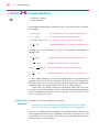
The graphs of f, f 1, and y x are shown in Figure 10. Sometimes it is difficult to visualize the reflection of the graph of f in the line y x. Choosing some
points on the graph of f and plotting their reflections first makes it easier to sketch
the graph of f 1. Figure 11 shows a check on a graphing utility.
y
5
5
yx
y f (x)
7.6
x
5
y
f 1(x)
5
FIGURE 10
Matched Problem 3
7.6
FIGURE 11
Find the inverse of f(x) 4x x2, x 2. Graph f, f 1, and y x in the same
coordinate system.
Answers to Matched Problems
1. (A) Not one-to-one
(B) One-to-one
2. f 1(x) x2 2, x 0
3. f 1(x) 2 4 x, x 4
y
y f 1(x)
yx
5
5
5
5
y f (x)
x
2-6
EXERCISE
2-6
A
10.
g (x)
Which of the functions in Problems 1–16 are one-to-one?
1. {(1, 2), (2, 1), (3, 4), (4, 3)}
2. {(1, 0), (0, 1), (1, 1), (2, 1)}
x
3. {(5, 4), (4, 3), (3, 3), (2, 4)}
4. {(5, 4), (4, 3), (3, 2), (2, 1)}
5. Domain
Range
6. Domain
2
4
2
1
2
1
0
0
0
1
1
1
Range
11.
h (x)
3
7
x
9
2
5
7. Domain
Range
8. Domain
Range
1
1
5
2
2
3
3
1
4
4
2
5
5
4
3
9.
2
7
f(x)
12.
x
13.
x
k (x)
m (x)
x
Inverse Functions
195
196
2 Graphs and Functions
14.
n (x)
29. f (x) x3 9x
x2 9
30. f (x) 4x x3
x2 4
In Problems 31–34, use the graph of the one-to-one function
f to sketch the graph of f 1. State the domain and
range of f 1.
x
y
31.
yx
5
y f (x)
15.
r(x)
5
5
x
5
x
y
32.
yx
5
16.
5
s(x)
5
x
y f (x)
5
x
y
33.
yx
5
5
y f (x)
5
x
B
5
Which of the functions in Problems 17–22 are one-to-one?
17. F(x) 12 x 2
18. G(x) 13 x 1
19. H(x) 4 x2
20. K(x) 4 x
21. M(x) x 1
22. N(x) x2 1
Problems 23–30 require the use of a graphing utility. Graph
each function, and use the graph to determine if the function
is one-to-one.
23. f (x) x2 x
x
25. f (x) x x
x
26. f (x) 27. f (x) x2 4
x2
28. f (x) 3
24. f (x) x2 x
x
x
3
x
x
1 x2
x1
y
34.
yx
5
5
5
x
5
In Problems 35–40, verify that g is the inverse of the
one-to-one function f by showing that g[ f(x)] x and
f [g(x)] x. Sketch the graphs of f, g, and the line y x
in the same coordinate system.
2-6
Inverse Functions
197
Check your graphs in Problems 35–40 by graphing f, g, and
the line y x in a squared viewing window on a graphing
utility.
69. f (x) 9 x2, 3 x 0
35. f (x) 3x 6; g(x) 13 x 2
The graph of each function in Problems 71–74 is one-quarter of the graph of the circle with radius 1 and center (0, 1).
Find f 1, find the domain and range of f 1, and sketch the
graphs of f and f 1 in the same coordinate system.
36. f (x) 12 x 2; g(x) 2x 4
37. f (x) 4 x2, x 0; g(x) x 4
70. f (x) 9 x2, 3 x 0
38. f (x) x 2; g(x) x2 2, x 0
71. f (x) 1 1 x2, 0 x 1
39. f (x) x 2; g(x) x2 2, x 0
72. f (x) 1 1 x2, 0 x 1
40. f (x) 6 x2, x 0; g(x) 6 x
73. f (x) 1 1 x2, 1 x 0
The functions in Problems 41–60 are one-to-one. Find f 1.
74. f (x) 1 1 x2, 1 x 0
41. f(x) 15 x
42. f(x) 4x
75. Find f 1(x) for f (x) ax b, a 0.
43. f(x) 2x 7
44. f(x) 0.25x 2.25
76. Find f 1(x) for f (x) a2 x2, a 0, 0 x a.
45. f(x) 0.2x 0.4
46. f(x) 7 8x
77. Refer to Problem 75. For which a and b is f its own inverse?
47. f(x) 3 2
x
48. f(x) 5 4
x
49. f(x) 2x
x1
50. f(x) 4x
2x
51. f(x) 0.2x 0.4
0.1x 0.5
52. f(x) x 0.2
x 0.5
53. f(x) 8x3 5
54. f(x) 2x5 9
5
55. f (x) 2 3x 7
3
56. f (x) 1 4 5x
57. f (x) 2 9 x
58. f (x) 3 x 4
59. f (x) 2 3 x
60. f (x) 4 x 5
61. How are the x and y intercepts of a function and its inverse
related?
78. How could you recognize the graph of a function that is its
own inverse?
79. Show that the line through the points (a, b) and (b, a),
a b, is perpendicular to the line y x (see the figure).
80. Show that the point ((a b)/2, (a b)/2) bisects the line
segment from (a, b) to (b, a), a b (see the figure).
y
yx
(a, b)
a 2 b , a 2 b (b, a)
x
62. Does a constant function have an inverse? Explain.
In Problems 81–84, the function f is not one-to-one. Find
the inverses of the functions formed by restricting the
domain of f as indicated.
C
The functions in Problems 63–66 are one-to-one. Find f 1.
63. f(x) (x 1)2 2, x 1
64. f(x) 3 (x 5)2, x 5
65. f(x) x2 2x 2, x 1
66. f(x) x2 8x 7, x 4
The graph of each function in Problems 67–70 is one-quarter of the graph of the circle with radius 3 and center (0, 0).
Find f 1, find the domain and range of f 1, and sketch the
graphs of f and f 1 in the same coordinate system.
67. f (x) 9 x2, 0 x 3
68. f (x) 9 x , 0 x 3
2
Check Problems 81–84 by graphing f, g, and the line y x
in a squared viewing window on a graphing utility. [Hint:
To restrict the graph of y f(x) to an interval of the form
a x b, enter y f(x)/((a x)* (x b)).]
81. f(x) (2 x)2:
(A) x 2
(B) x 2
82. f(x) (1 x)2:
(A) x 1
(B) x 1
83. f (x) 4x x2:
(A) 0 x 2
(B) 2 x 4
84. f (x) 6x x2:
(A) 0 x 3
(B) 3 x 6
198
2 Graphs and Functions
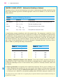
CHAPTER 2 GROUP ACTIVITY Mathematical Modeling in Business*
This group activity is concerned with analyzing a basic model for manufacturing and selling a product by using
tables of data and linear regression to determine appropriate values for the constants a, b, m, and n in the following functions:
TABLE 1 Business Modeling Functions
Function
Definition
Interpretation
Price–demand
p(x) m nx
x is the number of items that can be sold at $ p per item
Cost
C(x) a bx
Total cost of producing x items
Revenue
R(x) xp
Total revenue from the sale of x items
x(m nx)
P(x) R(x) C(x)
Profit
Total profit from the sale of x items
A manufacturing company manufactures and sells mountain bikes. The management would like to have
price–demand and cost functions for break-even and profit–loss analysis. Price–demand and cost functions may
be established by collecting appropriate data at different levels of output, and then finding a model in the form
of a basic elementary function (from our library of elementary functions) that “closely fits” the collected data.
The financial department, using statistical techniques, arrived at the price–demand and cost data in Tables 2
and 3, where p is the wholesale price of a bike for a demand of x thousand bikes and C is the cost, in thousands of dollars, of producing and selling x thousand bikes.
–Demand
TABLE 2 Price–
x (thousand)
p($)
TABLE 3 Cost
x (thousand)
C (thousand $)
7
530
5
2,100
13
360
12
2,940
19
270
19
3,500
25
130
26
3,920
(A) Building a Mathematical Model for Price–Demand. Plot the data in Table 2 and observe that the relationship between p and x is almost linear. After observing a relationship between variables, analysts often try
to model the relationship in terms of a basic function, from a portfolio of elementary functions, which “best
fits” the data.
1. Linear regression lines are frequently used to model linear phenomena. This is a process of fitting to a set
of data a straight line that minimizes the sum of the squares of the distances of all the points in the graph
of the data to the line by using the method of least squares. Many graphing utilities have this routine built
in. Read your user’s manual for your particular graphing utility, and discuss among the members of the
*This group project may be done without the use of a graphing utility, but significant additional insight into mathematical modeling will
be gained if one is available.
Chapter 2 Group Activity
199
group how this is done. After obtaining the linear regression line for the data in Table 2, graph the line and
the data in the same viewing window.
2. The linear regression line found in part 1 is a mathematical model for the price–demand function and is
given by
p(x) 666.5 21.5x
Price–demand function
Graph the data points from Table 2 and the price–demand function in the same rectangular coordinate
system.
3. The linear regression line defines a linear price–demand function. Interpret the slope of the function. Discuss its domain and range. Using the mathematical model, determine the price for a demand of 10,000 bikes.
For a demand of 20,000 bikes.
(B) Building a Mathematical Model for Cost. Plot the data in Table 3 in a rectangular coordinate system.
Which type of function appears to best fit the data?
1. Fit a linear regression line to the data in Table 3. Then plot the data points and the line in the same viewing window.
2. The linear regression line found in part 1 is a mathematical model for the cost function and is given by
C(x) 86x 1,782
Cost function
Graph the data points from Table 3 and the cost function in the same rectangular coordinate system.
3. Interpret the slope and the y intercept of the cost function. Discuss its domain and range. Using the mathematical model, determine the cost for an output and sales of 10,000 bikes. For an output and sales of 20,000
bikes.
(C) Break-Even and Profit–Loss Analysis. Write an equation for the revenue function and state its domain.
Write the equation for the profit function and state its domain.
1. Graph the revenue function and the cost function simultaneously in the same rectangular coordinate system.
Algebraically determine at what outputs (to the nearest unit) the company breaks even. Determine where
costs exceed revenues and revenues exceed costs.
2. Graph the revenue function and the cost function simultaneously in the same viewing window. Graphically
determine at what outputs (to the nearest unit) the company breaks even and where costs exceed revenues
and revenues exceed costs.
3. Graph the profit function in a rectangular coordinate system. Algebraically determine at what outputs (to the
nearest unit) the company breaks even. Determine where profits occur and where losses occur. At what output and price will a maximum profit occur? Do the maximum revenue and maximum profit occur for the
same output? Discuss.
4. Graph the profit function in a graphing utility. Graphically determine at what outputs (to the nearest unit)
the company breaks even and where losses occur and profits occur. At what output and price will a maximum profit occur? Do the maximum revenue and maximum profit occur for the same output? Discuss.