Download - CambridgeSoft

ChemOffice.Com
®
ChemOffice
®
Chem3D, ChemFinder and E-Notebook
User’s Guide
Revision 9.0.1
12/22/04
CS Chem3D 9.0
for Windows
Chem3D is a stand alone application within
ChemOffice, an integrated suite including
ChemDraw for Chemical Structure Drawing
ChemFinder for searching and information integration,
BioAssay for biological data retrieval and visualization,
Inventory for managing and searching reagents,
E-Notebook for electronic journal and information, and
ChemInfo for chemical and reference databases.
Chem3D
®
Molecular Modeling and Analysis Standard
License Information
ChemOffice, ChemDraw, Chem3D, ChemFinder, and ChemInfo programs, all resources in the ChemOffice,
ChemDraw, Chem3D, ChemFinder, and ChemInfo application files, and this manual are Copyright © 1986-2004
by CambridgeSoft Corporation (CS) with all rights reserved worldwide. MOPAC 2000 and MOPAC 2002 are
Copyright © 1993-2004 by Fujitsu Limited with all rights reserved. Information in this document is subject to
change without notice and does not represent a commitment on the part of CS. Both these materials and the right
to use them are owned exclusively by CS. Use of these materials is licensed by CS under the terms of a software license
agreement; they may be used only as provided for in said agreement.
ChemOffice, ChemDraw, Chem3D, CS MOPAC, ChemFinder, Inventory, E-Notebook, BioAssay, and ChemInfo
are not supplied with copy protection. Do not duplicate any of the copyrighted materials except for your personal
backups without written permission from CS. To do so would be in violation of federal and international law, and
may result in criminal as well as civil penalties. You may use ChemOffice, ChemDraw, Chem3D, CS MOPAC,
ChemFinder, Inventory, E-Notebook, BioAssay, and ChemInfo on any computer owned by you; however, extra
copies may not be made for that purpose. Consult the CS License Agreement for Software and Database Products
for further details.
Trademarks
ChemOffice, ChemDraw, Chem3D, ChemFinder, ChemInfo and ChemACX are registered trademarks of
CambridgeSoft Corporation (Cambridge Scientific Computing, Inc.).
The Merck Index is a registered trademark of Merck & Co., Inc. ©2001 All rights reserved.
MOPAC 2000 and MOPAC 2002 are trademarks of Fujitsu Limited.
Microsoft Windows, Windows NT, Windows 95, and Microsoft Word are registered trademarks of Microsoft Corp.
Apple Events, Macintosh, Laserwriter, Imagewriter, QuickDraw and AppleScript are registered trademarks of Apple
Computer, Inc. Geneva, Monaco, and TrueType are trademarks of Apple Computer, Inc.
The ChemSelect Reaction Database is copyrighted © by InfoChem GmbH 1997.
AspTear is copyrighted © by Softwing.
Copyright © 1986-2004 CambridgeSoft Corporation (Cambridge Scientific Computing, Inc.) All Rights Reserved.
Printed in the United States of America.
All other trademarks are the property of their respective holders.
CambridgeSoft End-User License Agreement for Software Products
Important: This CambridgeSoft Software License Agreement (“Agreement”) is a legal agreement between you, the
end user (either an individual or an entity), and CambridgeSoft Corporation (“CS”) regarding the use of CS Software
Products, which may include computer software, the associated media, any printed materials, and any “online” or
electronic documentation. By installing, copying, or otherwise using any CS Software Product, you signify that you
have read the CS End User License Agreement and agree to be bound by its terms. If you do not agree to the
Agreement’s terms, promptly return the package and all its contents to the place of purchase for a full refund.
CambridgeSoft Software License
1. Grant of License. CambridgeSoft (CS) Software Products are licensed, not sold. CS grants and you hereby accept
a nonexclusive license to use one copy of the enclosed Software Product (“Software”) in accordance with the terms
of this Agreement. This licensed copy of the Software may only be used on a single computer, except as provided
below. You may physically transfer the Software from one computer to another for your own use, provided the
Software is in use (or installed) on only one computer at a time. If the Software is permanently installed on your computer (other than a network server), you may also use the Software on a portable or home computer, provided that
you use the software on only one computer at a time. You may not (a) electronically transfer the Software from one
computer to another, (b) distribute copies of the Software to others, or (c) modify or translate the Software without
the prior written consent of CS, (d) place the software on a server so that it is accessible via a public network such as
the Internet, (e) sublicense, rent, lease or lend any portion of the Software or Documentation, (f ) modify or adapt
the Software or merge it into another program, (g) modify or circumvent the software activation, or (h) reverse engineer the software activation so as to circumvent it. The Software may be placed on a file or disk server connected to
a network, provided that a license has been purchased for every computer with access to that server. You may make
only those copies of the Software which are necessary to install and use it as permitted by this agreement, or are for
purposes of backup and archival records; all copies shall bear CS’s copyright and proprietary notices. You may not
make copies of any accompanying written materials.
With a fixed license, the software cannot be installed on more than the number of computers equivalent to the number of fixed licenses purchased. For example, a 10-user fixed license means the software can be installed on no more
than 10 different computers. A fixed license cannot be installed on a server. With a concurrent license, the software
can be installed on any number of computers at the organization, but the number of computers using the software
at any one time cannot exceed the number of concurrent licenses purchased. For example, a 10-user concurrent
license can be installed on 20 computers, but no more than 10 users can be using it at any one time. If the number
of users of the software could potentially exceed the number of licensed copies, then Licensee must have a reasonable
mechanism or process in place to assure that the number of persons using the software does not exceed the number
of copies. CambridgeSoft reserves the right to conduct periodic audits no more than once per year to review the
implementation of this agreement at the Licensee’s site. At CambridgeSoft’s request, Licensee will provide a knowledgeable employee to assist in said audit
2. Ownership. The Software is and at all times shall remain the sole property of CS. This ownership is protected by
the copyright laws of the United States and by international treaty provisions. Upon expiration or termination of this
agreement, you shall promptly return all copies of the Software and accompanying written materials to CS. You may
not modify, decompile, reverse engineer, or disassemble the Software.
3. Assignment Restrictions. You may not rent, lease, or otherwise sublet the Software or any part thereof. You may
transfer on a permanent basis the rights granted under this license provided you transfer this Agreement and all copies
of the Software, including prior versions, and all accompanying materials. The recipient must agree to the terms of
this Agreement in full and register this transfer in writing with CS.
4. Use of Included Data. All title and copyrights in and to the Software product, including but not limited to any
images, photographs, animations, video, audio, music, text, applets, Java applets, and data files and databases (the
“Included Data”), are owned by CS or its suppliers.
· You may not copy, distribute or otherwise make the Included Data publicly available.
· Licensed users of ChemOffice Enterprise and Workgroup and the accompanying Plugin software products may
access, search, and view the Included Data and may transmit the results of any search of the Included Data to other
users of the licensed ChemOffice Enterprise and Workgroup software products within your organization only, provided
that such transmission is via an internal corporate (or university) network and is not accessible by the public.
· You may not install the Included Data on non-licensed computers nor distribute or otherwise make the Included
Data publicly available.
· You may use the Software to organize personal data, and you may transmit such personal data over the Internet provided that the transmission does not contain any Included Data.
· All rights not specifically granted under this Agreement are reserved by CS.
5. Separation of Components. The Software is licensed as a single product. Its component parts may not be separated for use on more than one computer, except in the case of ChemOffice Enterprise. ChemOffice Enterprise
includes licenses for ChemDraw ActiveX and licenses for Chem3D ActiveX. The ActiveX software products may be
installed on computers other than that one on which ChemOffice Enterprise is installed. However, each copy of the
ActiveX is individually subject to the provisions of Paragraphs 1 through 4 of this Agreement.
6. Educational Use Only of Student Licenses. If you are a student enrolled at an educational institution, the CS
License Agreement grants to you personally a license to use one copy of the enclosed Software in accordance with the
terms of this Agreement. In this case the CS License Agreement does not permit commercial use of the Software nor
does it permit you to allow any other person to use the Software.
7. Termination. You may terminate the license at any time by destroying all copies of the Software and documentation in your possession. Without prejudice to any other rights, CS may terminate this Agreement if you fail to comply with its terms and conditions. In such event, you must destroy all copies of the Software Product and all of its
component parts.
8. Confidentiality. The Software contains trade secrets and proprietary know-how that belong to CS and are
being made available to you in strict confidence. ANY USE OR DISCLOSURE OF THE SOFTWARE, OR USE OF ITS
ALGORITHMS, PROTOCOLS OR INTERFACES, OTHER THAN IN STRICT ACCORDANCE WITH THIS LICENSE
AGREEMENT, MAY BE ACTIONABLE AS A VIOLATION OF OUR TRADE SECRET RIGHTS.
CS Limited Warranty
Limited Warranty. CS’s sole warranty with respect to the Software is that it shall be free of errors in program logic
or documentation, attributable to CS, which prevent the performance of the principal computing functions of the
Software. CS warrants this for a period of thirty (30) days from the date of receipt.
CS’s Liability. In no event shall CS be liable for any indirect, special, or consequential damages, such as, but not
limited to, loss of anticipated profits or other economic loss in connection with or arising out of the use of the software by you or the services provided for in this agreement, even if CS has been advised of the possibility of such damages. CS’s entire liability and your exclusive remedy shall be, at CS’s discretion, either (A) return of any license fee,
or (B) correction or replacement of software that does not meet the terms of this limited warranty and that is returned
to CS with a copy of your purchase receipt.
NO OTHER WARRANTIES. CS DISCLAIMS OTHER IMPLIED WARRANTIES, INCLUDING, BUT NOT LIMITED TO,
IMPLIED WARRANTIES OF MERCHANTABILITY OR FITNESS FOR A PARTICULAR PURPOSE, AND IMPLIED WARRANTIES ARISING BY USAGE OF TRADE, COURSE OF DEALING, OR COURSE OF PERFORMANCE. NOTWITH-
STANDING THE ABOVE, WHERE APPLICABLE, IF YOU QUALIFY AS A “CONSUMER” UNDER THE MAGNUSONMOSS WARRANTY ACT, THEN YOU MAY BE ENTITLED TO ANY IMPLIED WARRANTIES ALLOWED BY LAW FOR
THE PERIOD OF THE EXPRESS WARRANTY AS SET FORTH ABOVE. SOME STATES DO NOT ALLOW LIMITATIONS
ON IMPLIED WARRANTIES, SO THE ABOVE LIMITATION MIGHT NOT APPLY TO YOU. THIS WARRANTY GIVES
YOU SPECIFIC LEGAL RIGHTS, AND YOU MAY ALSO HAVE OTHER RIGHTS WHICH VARY FROM STATE TO STATE.
No Waiver. The failure of either party to assert a right hereunder or to insist upon compliance with any term or condition of this Agreement shall not constitute a waiver of that right or excuse a similar subsequent failure to perform
any such term or condition by the other party.
Governing Law. This Agreement shall be construed according to the laws of the Commonwealth of Massachusetts.
Export. You agree that the Software will not be shipped, transferred, or exported into any country or used in any manner prohibited by the United States Export Administration Act or any other export laws, restrictions, or regulations.
End-User License Agreement for CambridgeSoft Database Products
Important: This CambridgeSoft End-User License Agreement is a legal agreement between you (either an individual or a single entity) and CambridgeSoft Corporation for the CambridgeSoft supplied database product(s) and may
include associated media, printed materials, and “online” or electronic documentation. By using the database product(s) you agree that you have read, understood and will be bound by this license agreement.
Database Product License
1. Copyright Notice. The materials contained in CambridgeSoft Database Products, including but not limited to,
ChemACX, ChemIndex, and The Merck Index, are protected by copyright laws and international copyright treaties,
as well as other intellectual property laws and treaties. Copyright in the materials contained on the CD and internet
subscription products, including, but not limited to, the textual material, chemical structures representations,
artwork, photographs, computer software, audio and visual elements, is owned or controlled separately by
CambridgeSoft Corporation (“CS”).
CS is a distributor (and not a publisher) of information supplied by third parties. Accordingly, CS has no editorial
control over such information. Database Suppliers (“Supplier”) individually own all right, title, and interest, including copyright, in their database—and retain all such rights in providing information to Customers.
The materials contained in The Merck Index are protected by copyright laws and international copyright treaties, as
well as other intellectual property laws and treaties. Copyright in the materials contained on the CD and internet
subscription products, including, but not limited to, the textual material, chemical structures representations, artwork, photographs, computer software, audio and visual elements, is owned or controlled separately by the Merck &
Co., Inc., (“Merck”) and CambridgeSoft Corporation (“CS”).
2. Limitations on Use. Except as expressly provided by copyright law, copying, redistribution, or publication,
whether for commercial or non-commercial purposes, must be with the express permission of CS and/or Merck. In
any copying, redistribution, or publication of copyrighted material, any changes to or deletion of author attribution
or copyright notice, or any other proprietary notice of CS, Merck, or other Database producer are prohibited.
3. Grant of License, CD/DVD Databases. CambridgeSoft Software Products are licensed, not sold. CambridgeSoft
grants and you hereby accept a nonexclusive license to use one copy of the enclosed Software Product (“Software”)
in accordance with the terms of this Agreement. This licensed copy of the Software may only be used on a single
computer, except as provided below. You may physically transfer the Software from one computer to another for your
own use, provided the Software is in use (or installed) on only one computer at a time. If the Software is permanently
installed on your computer (other than a network server), you may also use the Software on a portable or home comSoftware from one computer to another, (b) distribute copies of the Software to others, or (c) modify or translate the
Software without the prior written consent of CambridgeSoft, (d) place the software on a server so that it is accessible via a public network such as the Internet, (e) sublicense, rent, lease or lend any portion of the Software or
Documentation, or (f ) modify or adapt the Software or merge it into another program. The Software may be placed
on a file or disk server connected to a network, provided that a license has been purchased for every computer with
access to that server. You may make only those copies of the Software which are necessary to install and use it as permitted by this agreement, or are for purposes of backup and archival records; all copies shall bear CambridgeSoft’s
copyright and proprietary notices. You may not make copies of any accompanying written materials.
4. Assignment Restrictions for CD/DVD databases. You may not rent, lease, or otherwise sublet the Software or
any part thereof. You may transfer on a permanent basis the rights granted under this license provided you transfer
this Agreement and all copies of the Software, including prior versions, and all accompanying materials. The recipient must agree to the terms of this Agreement in full and register this transfer in writing with CambridgeSoft.
5. Revocation of Subscription Access. Any use which is commercial and/or non-personal is strictly prohibited, and
may subject the Subscriber making such uses to revocation of access to this Paid Subscription Service, as well as any
other applicable civil or criminal penalties. Similarly, sharing a Subscriber password with a non-Subscriber or otherwise making this Paid Subscription Service available to third parties other than the Authorized User as defined above
is strictly prohibited, and may subject the Subscriber participating in such activities to revocation of access to the Paid
Subscription Services; and, the Subscriber and any third party, to any other applicable civil or criminal penalties
under copyright or other laws. In the case of an authorized site license, a Subscriber shall cause any employee, agent
or other third party which the Subscriber allows to use the Paid Subscription Service materials to abide by all of the
terms and conditions of this Agreement. In all other cases, only the Subscriber is permitted to access the Paid
Subscription Service materials. Should CambridgeSoft become aware of any use that might cause revocation of the
license, they shall notify the Subscriber. The Subscriber shall have 90 days from date of notice to correct such violation before any action will be taken.
6. Trademark Notice. THE MERCK INDEX ® is a trademark of Merck & Company Incorporated, Whitehouse
Station, New Jersey, USA and is registered in the United States Patent and Trademark Office. CambridgeSoft ® and
ChemACX are trademarks of CambridgeSoft Corporation, Cambridge,Massachusetts, USA and are registered in the
United States Patent and Trademark Office, the European Union (CTM) and Japan.
Any use of the marks in connection with the sale, offering for sale, distribution or advertising of any goods and services, including any other website, or in connection with labels, signs, prints, packages, wrappers, receptacles or
advertisements used for the sale, offering for sale, distribution or advertising of any goods and services, including any
other website, which is likely to cause confusion, to cause mistake or to deceive, is strictly prohibited.
7. Modification of Databases, Websites, or Subscription Services. CS reserves the right to change, modify, suspend or discontinue any or all parts of any Paid Subscription Services and databases at any time.
8. Representations and Warranties. The User shall indemnify, defend and hold CS, Merck, and/or other Supplier
harmless from any damages, expenses and costs (including reasonable attorneys’ fees) arising out of any breach or
alleged breach of these Terms and Conditions, representations and/or warranties herein, by the User or any third
party to whom User shares her/his password or otherwise makes available this Subscription Service. The User shall
cooperate in the defense of any claim brought against CambridgeSoft, Merck, and/or other Database Suppliers.
In no event shall CS, Merck, and/or other Supplier be liable for any indirect, special, or consequential damages, such
as, but not limited to, loss of anticipated profits or other economic loss in connection with or arising out of the use
of the software by you or the services provided for in this agreement, even if CS, Merck, and/or other Supplier has
been advised of the possibility of such damages. CS and/or Merck’s entire liability and your exclusive remedy shall
be, at CS’s discretion a return of any pro-rata portion of the subscription fee.
The failure of either party to assert a right hereunder or to insist upon compliance with any term or condition of this
Agreement shall not constitute a waiver of that right or excuse a similar subsequent failure to perform any such term
or condition by the other party.
This Agreement shall be construed according to the laws of the Commonwealth of Massachusetts, United States of
America.
: IS IT OK TO COPY MY COLLEAGUE’S
SOFTWARE?
NO, it’s not okay to copy your colleague’s
software. Software is protected by federal copyright law,
which says that you can't make such additional copies
without the permission of the copyright holder. By
protecting the investment of computer software
companies in software development, the copyright law
serves the cause of promoting broad public availability of
new, creative, and innovative products. These companies
devote large portions of their earnings to the creation of
new software products and they deserve a fair return on
their investment. The creative teams who develop the
software–programmers, writers, graphic artists and
others–also deserve fair compensation for their efforts.
Without the protection given by our copyright laws, they
would be unable to produce the valuable programs that
have become so important to our daily lives: educational
software that teaches us much needed skills; business
software that allows us to save time, effort and money;
and entertainment and personal productivity software
that enhances leisure time.
Q
Q: That makes sense, but what do I get out of
purchasing my own software?
A: When you purchase authorized copies of software
programs, you receive user guides and tutorials, quick
reference cards, the opportunity to purchase
upgrades, and technical support from the software
publishers. For most software programs, you can read
about user benefits in the registration brochure or
upgrade flyer in the product box.
Q: What exactly does the law say about copying
software?
A: The law says that anyone who purchases a copy of
software has the right to load that copy onto a single
computer and to make another copy “for archival
purposes only” or, in limited circumstances, for
“purposes only of maintenance or repair.” It is illegal
to use that software on more than one computer or to
make or distribute copies of that software for any
other purpose unless specific permission has been
obtained from the copyright owner. If you pirate
software, you may face not only a civil suit for
damages and other relief, but criminal liability as well,
including fines and jail terms of up to one year
Q: So I'm never allowed to copy software for any other
reason?
A: That’s correct. Other than copying the software you
purchase onto a single computer and making another
copy “for archival purposes only” or “purposes only of
maintenance or repair,” the copyright law prohibits
you from making additional copies of the software for
any other reason unless you obtain the permission of
the software company.
Q: At my company, we pass disks around all the time.
We all assume that this must be okay since it was
the company that purchased the software in the
first place.
A: Many employees don’t realize that corporations are
bound by the copyright laws, just like everyone else.
Such conduct exposes the company (and possibly the
persons involved) to liability for copyright
infringement. Consequently, more and more
corporations concerned about their liability have
written policies against such “softlifting”. Employees
may face disciplinary action if they make extra copies
of the company’s software for use at home or on
additional computers within the office. A good rule to
remember is that there must be one authorized copy
of a software product for every computer upon which
it is run
Q: Can I take a piece of software owned by my
company and install it on my personal computer at
home if instructed by my supervisor?
A: A good rule of thumb to follow is one software
package per computer, unless the terms of the license
agreement allow for multiple use of the program. But
some software publishers’ licenses allow for “remote”
or “home” use of their software. If you travel or
telecommute, you may be permitted to copy your
software onto a second machine for use when you are
not at your office computer. Check the license carefully to see if you are allowed to do this.
Q: What should I do if become aware of a company
that is not compliant with the copyright law or its
software licenses?
A: Cases of retail, corporate and Internet piracy or noncompliance with software licenses can be reported on
the Internet at http://www.siia.net/piracy/report.asp
or by calling the Anti-Piracy Hotline:
(800) 388-7478.
Q: Do the same rules apply to bulletin boards and user
groups? I always thought that the reason they got
together was to share software.
A: Yes. Bulletin boards and user groups are bound by the
copyright law just as individuals and corporations.
However, to the extent they offer shareware or public
domain software, this is a perfectly acceptable
practice. Similarly, some software companies offer
bulletin boards and user groups special demonstration
versions of their products, which in some instances
may be copied. In any event, it is the responsibility of
the bulletin board operator or user group to respect
copyright law and to ensure that it is not used as a
vehicle for unauthorized copying or distribution.
Q: I'll bet most of the people who copy software don't
even know that they're breaking the law.
A: Because the software industry is relatively new, and
because copying software is so easy, many people are
either unaware of the laws governing software use or
choose to ignore them. It is the responsibility of each
and every software user to understand and adhere to
copyright law. Ignorance of the law is no excuse. If
you are part of an organization, see what you an do to
initiate a policy statement that everyone respects.
Also, suggest that your management consider
conducting a software audit. Finally, as an individual,
help spread the word that users should be “software
legal.”
Q: What are the penalties for copyright infringement?
A: The Copyright Act allows a copyright owner to
recover monetary damages measured either by: (1) its
actual damages plus any additional profits of the
infringer attributable to the infringement, or (2)
statutory damages, of up to $150,000 for each copyrighted work infringed. The copyright owner also has
the right to permanently enjoin an infringer from
engaging in further infringing activities and may be
awarded costs and attorneys’ fees. The law also
permits destruction or other reasonable disposition of
all infringing copies and devices by which infringing
copies have been made or used in violation of the
copyright owner’s exclusive rights. In cases of willful
infringement, criminal penalties may also be assessed
against the infringer.
SIIA also offers a number of other materials designed to
help you comply with the Federal Copyright Law. These
materials include:
"It's Just Not Worth the Risk" video.
This 12–minute video, available $10, has helped over
20,000 organizations dramatize to their employees the
implications and consequences of software piracy.
“Don’t Copy that Floppy” video
This 9 minute rap video, available for $10, is designed
to educate students on the ethical use of software.
Other education materials including, “Software Use
and the Law”, a brochure detailing the copyright law
and how software should be used by educational
institutions, corporations and individuals; and several
posters to help emphasize the message that unauthorized
copying of software is illegal.
To order any of these materials, please send your request to:
“SIIA Anti-Piracy Materials”
Software & Information Industry Association
1090 Vermont Ave, Sixth Floor,
Washington, D.C. 20005
(202) 289-7442
We urge you to make as many copies as you would like
in order to help us spread the word that unauthorized
copying of software is illegal.
A Guide to CambridgeSoft Manuals
Includes
ChemDraw
Software
Chem3D
ChemFinder
E-Notebook Desktop
Inventory Desktop
Desktop Applications
BioAssay Desktop
ChemDraw/Excel
ChemFinder/Office
CombiChem/Excel
ChemSAR/Excel
MOPAC, MM2
CS Gaussian, GAMESS Interface
ChemOffice WebServer
Oracle Cartridge
Enterprise Solutions
E-Notebook Workgroup, Enterprise
Document Manager
Registration Enterprise
Formulations & Mixtures
Inventory Workgroup, Enterprise
Discovery LIMS
BioAssay Workgroup, Enterprise
BioSAR Enterprise
ChemDraw/Spotfire
Databases
The Merck Index
ChemACX, ChemSCX
ChemMSDX
ChemINDEX, NCI & AIDS
ChemRXN
Ashgate Drugs
Tips
Structure Drawing Tips
Searching Tips
Importing SD Files
C
Dr
C
aw hem he
M
in
m
i
g cal
an
D
St
St
a
r
ua
nd uc ra
tu
a
rd
re w
ls
Ch
em
O
ffi
ce
Ch
em
& 3D,
EN Che
ot
eb mFi
oo nd
er
k
Ch
em
O
ffi
ce
En
t
An erp
ri
d
Da se S
o
ta
ba luti
se on
s
s
Contents
Introduction
About CS MOPAC . . . . . . . . . . . . . . . . . . . . . . . 9
About Gaussian . . . . . . . . . . . . . . . . . . . . . . . . . . 9
About CS Mechanics . . . . . . . . . . . . . . . . . . . . . 9
What’s New in Chem3D 9.0? . . . . . . . . . . . . 10
What’s New in Chem3D 9.0.1? . . . . . . . . . . . . . 10
For Users of Previous Versions of Chem3D. . . 11
CambridgeSoft Web Pages . . . . . . . . . . . . . . . . . 11
Installation and System Requirements . . . 11
Microsoft®Windows® Requirements . . . . . . . . 11
Site License Network Installation Instructions . 12
Chapter 1: Chem3D Basics
The Graphical User Interface . . . . . . . . . . . 13
Model Window . . . . . . . . . . . . . . . . . . . . . . . . . . 13
Rotation Bars. . . . . . . . . . . . . . . . . . . . . . . . . . . 14
Menus and Toolbars . . . . . . . . . . . . . . . . . . . . . . 14
The File Menu . . . . . . . . . . . . . . . . . . . . . . . . . . 14
The Edit Menu . . . . . . . . . . . . . . . . . . . . . . . . . 15
The View Menu/Model Display Toolbar. . . . . . 15
The Structure Menu. . . . . . . . . . . . . . . . . . . . . . 17
The Standard Toolbar . . . . . . . . . . . . . . . . . . . . 19
The Building Toolbar . . . . . . . . . . . . . . . . . . . . 20
The Model Display Toolbar. . . . . . . . . . . . . . . . 20
The Surfaces Toolbar . . . . . . . . . . . . . . . . . . . . 21
The Movie Toolbar . . . . . . . . . . . . . . . . . . . . . . 21
The Calculation Toolbar . . . . . . . . . . . . . . . . . . 22
The ChemDraw Panel . . . . . . . . . . . . . . . . . . . . 22
The Model Information Panel . . . . . . . . . . . . . . 23
The Output and Comments Windows . . . . . . . 23
Model Building Basics . . . . . . . . . . . . . . . . . . 24
Internal and External Tables . . . . . . . . . . . . . . . 24
The Model Setting Dialog Box . . . . . . . . . . . . . 25
Model Display . . . . . . . . . . . . . . . . . . . . . . . . . . . 25
Model Data Labels . . . . . . . . . . . . . . . . . . . . . . 26
Atom Types . . . . . . . . . . . . . . . . . . . . . . . . . . . 27
Rectification . . . . . . . . . . . . . . . . . . . . . . . . . . . 27
Bond Lengths and Bond Angles . . . . . . . . . . . . 27
The Model Explorer . . . . . . . . . . . . . . . . . . . . . . 27
Model Coordinates . . . . . . . . . . . . . . . . . . . . . . . 28
Z-matrix . . . . . . . . . . . . . . . . . . . . . . . . . . . . . . 28
Cartesian Coordinates . . . . . . . . . . . . . . . . . . . . 28
The Measurements Table. . . . . . . . . . . . . . . . . . 29
ChemOffice 2005/Chem3D
Chapter 2: Chem3D Tutorials
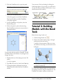
Tutorial 1: Working with ChemDraw . . . . 31
Tutorial 2: Building Models with the
Bond Tools . . . . . . . . . . . . . . . . . . . . . . . . . . . . 32
Tutorial 3: Building Models with the Text
Building Tool. . . . . . . . . . . . . . . . . . . . . . . . . . 36
Replacing Atoms. . . . . . . . . . . . . . . . . . . . . . . . . 37
Using Labels to Create Models . . . . . . . . . . . . . 37
Using Substructures . . . . . . . . . . . . . . . . . . . . . . 38
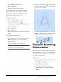
Tutorial 4: Examining Conformations . . 39
Tutorial 5: Mapping Conformations with
the Dihedral Driver . . . . . . . . . . . . . . . . . . . 42
Rotating two dihedrals . . . . . . . . . . . . . . . . . . . 43
Customizing the Graph . . . . . . . . . . . . . . . . . . 43
Tutorial 6: Overlaying Models . . . . . . . . . .
Tutorial 7: Docking Models . . . . . . . . . . . . .
Tutorial 8: Viewing Molecular Surfaces .
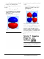
Tutorial 9: Mapping Properties onto
Surfaces . . . . . . . . . . . . . . . . . . . . . . . . . . . . . .
Tutorial 10: Computing Partial Charges .
43
46
48
49
52
Chapter 3: Displaying Models
Structure Displays . . . . . . . . . . . . . . . . . . . . . . 55
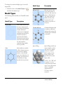
Model Types . . . . . . . . . . . . . . . . . . . . . . . . . . . . 56
Displaying Solid Spheres . . . . . . . . . . . . . . . . . . 57
Setting Solid Sphere Size. . . . . . . . . . . . . . . . . . 57
Displaying Dot Surfaces . . . . . . . . . . . . . . . . . . . 58
Coloring Displays . . . . . . . . . . . . . . . . . . . . . . . . 58
Coloring by Element . . . . . . . . . . . . . . . . . . . . 58
Coloring by Group . . . . . . . . . . . . . . . . . . . . . . 59
Coloring by Partial Charge . . . . . . . . . . . . . . . . 59
Coloring by depth for Chromatek stereo viewers 59
Red-blue Anaglyphs . . . . . . . . . . . . . . . . . . . . . 59
Depth Fading3D enhancement: . . . . . . . . . . . . 60
Perspective Rendering . . . . . . . . . . . . . . . . . . . 60
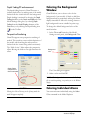
Coloring the Background Window . . . . . . . . . . 60
Coloring Individual Atoms. . . . . . . . . . . . . . . . . 60
Displaying Atom Labels . . . . . . . . . . . . . . . . . . . 61
Setting Default Atom Label Display Options . . 61
Displaying Labels Atom by Atom . . . . . . . . . . 61
Using Stereo Pairs . . . . . . . . . . . . . . . . . . . . . . . . 61
Using Hardware Stereo Graphic Enhancement 62
Molecular Surface Displays . . . . . . . . . . . . . 63
Extended Hückel . . . . . . . . . . . . . . . . . . . . . . . . 63
Displaying Molecular Surfaces . . . . . . . . . . . . . . 64
•
Administrator
Setting Molecular Surface Types . . . . . . . . . . . .
Setting Molecular Surface Isovalues . . . . . . . . .
Setting the Surface Resolution . . . . . . . . . . . . .
Setting Molecular Surface Colors . . . . . . . . . . .
Setting Solvent Radius . . . . . . . . . . . . . . . . . . .
Setting Surface Mapping . . . . . . . . . . . . . . . . . .
Solvent Accessible Surface . . . . . . . . . . . . . . . .
Connolly Molecular Surface . . . . . . . . . . . . . . .
Total Charge Density . . . . . . . . . . . . . . . . . . . . .
Total Spin Density . . . . . . . . . . . . . . . . . . . . . . .
Molecular Electrostatic Potential . . . . . . . . . . .
Molecular Orbitals . . . . . . . . . . . . . . . . . . . . . . .
Visualizing Surfaces from Other Sources
65
66
67
67
67
68
68
69
69
70
70
70
71
Chapter 4: Building and Editing Models
Setting the Model Building Controls . . . . 73
Building with the ChemDraw Panel . . . . . 74
Unsynchronized Mode . . . . . . . . . . . . . . . . . . . 74
Name=Struct . . . . . . . . . . . . . . . . . . . . . . . . . . . 75
Building with Other 2D Programs . . . . . . . . . . 75
Building With the Bond Tools . . . . . . . . . . 75
Creating Uncoordinated Bonds. . . . . . . . . . . . . 76
Removing Bonds and Atoms . . . . . . . . . . . . . . 76
Building With The Text Tool . . . . . . . . . . . 77
Using Labels . . . . . . . . . . . . . . . . . . . . . . . . . . . 77
Changing atom types . . . . . . . . . . . . . . . . . . . . 78
The Table Editor . . . . . . . . . . . . . . . . . . . . . . . 78
Specifying Order of Attachment . . . . . . . . . . . . 78
Using Substructures. . . . . . . . . . . . . . . . . . . . . . 78
Building with Substructures . . . . . . . . . . . . . . . 79
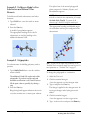
Example 1. Building Ethane with Substructures 79
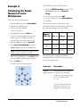
Example 2. Building a Model with a Substructure
and Several Other Elements 80
Example 3. Polypeptides. . . . . . . . . . . . . . . . . . 80
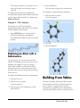
Example 4. Other Polymers . . . . . . . . . . . . . . . 81
Replacing an Atom with a Substructure . . . . . . 81
Building From Tables . . . . . . . . . . . . . . . . . . 81
Examples . . . . . . . . . . . . . . . . . . . . . . . . . . . . . . 82
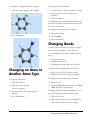
Changing an Atom to Another Element . 82
Changing an Atom to Another Atom Type 83
Changing Bonds . . . . . . . . . . . . . . . . . . . . . . . 83
Creating Bonds by Bond Proximate Addition . 84
Adding Fragments . . . . . . . . . . . . . . . . . . . . . 84
View Focus. . . . . . . . . . . . . . . . . . . . . . . . . . . . . 85
Setting Measurements . . . . . . . . . . . . . . . . . . 85
Setting Bond Lengths . . . . . . . . . . . . . . . . . . . .
Setting Bond Angles . . . . . . . . . . . . . . . . . . . . .
Setting Dihedral Angles . . . . . . . . . . . . . . . . . . .
Setting Non-Bonded Distances (Atom Pairs) .
Atom Movement When Setting Measurements
Setting Constraints. . . . . . . . . . . . . . . . . . . . . . .
•
86
86
86
86
86
87
Setting Charges . . . . . . . . . . . . . . . . . . . . . . . . . 87
Setting Serial Numbers . . . . . . . . . . . . . . . . . 88
Changing Stereochemistry . . . . . . . . . . . . . . 88
Inversion . . . . . . . . . . . . . . . . . . . . . . . . . . . . . . 88
Reflection . . . . . . . . . . . . . . . . . . . . . . . . . . . . . . 89
Refining a Model . . . . . . . . . . . . . . . . . . . . . . . 90
Rectifying Atoms . . . . . . . . . . . . . . . . . . . . . . . . 90
Cleaning Up a Model . . . . . . . . . . . . . . . . . . . . . 90
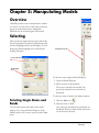
Chapter 5: Manipulating Models
Selecting. . . . . . . . . . . . . . . . . . . . . . . . . . . . . . . . 91
Selecting Single Atoms and Bonds . . . . . . . . . .
Selecting Multiple Atoms and Bonds . . . . . . . .
Deselecting Atoms and Bonds . . . . . . . . . . . . .
Selecting Groups of Atoms and Bonds . . . . . .
91
92
92
92
Using the Selection Rectangle. . . . . . . . . . . . . . . 92
Defining Groups . . . . . . . . . . . . . . . . . . . . . . . . 93
Selecting a Group or Fragment . . . . . . . . . . . . . 93
Selecting Atoms or Groups by Distance . . . . . 94
Showing and Hiding Atoms . . . . . . . . . . . . . 94
Showing Hs and Lps . . . . . . . . . . . . . . . . . . . . . 95
Showing All Atoms . . . . . . . . . . . . . . . . . . . . . . 95
Moving Atoms or Models . . . . . . . . . . . . . . . 95
Moving Models with the Translate Tool . . . . . . 96
Rotating Models . . . . . . . . . . . . . . . . . . . . . . . . 96
X- Y- or Z-Axis Rotations . . . . . . . . . . . . . . . . . 97
Rotating Fragments . . . . . . . . . . . . . . . . . . . . . . 97
Trackball Tool. . . . . . . . . . . . . . . . . . . . . . . . . . . 97
Internal Rotations . . . . . . . . . . . . . . . . . . . . . . . 97
Rotating Around a Bond . . . . . . . . . . . . . . . . . . 98
Rotating Around a Specific Axis . . . . . . . . . . . . 98
Rotating a Dihedral Angle . . . . . . . . . . . . . . . . . 98
Using the Rotation Dial . . . . . . . . . . . . . . . . . . . 99
Changing Orientation . . . . . . . . . . . . . . . . . . . 99
Aligning to an Axis . . . . . . . . . . . . . . . . . . . . . . 99
Aligning to a Plane . . . . . . . . . . . . . . . . . . . . . . . 99
Resizing Models . . . . . . . . . . . . . . . . . . . . . . . 100
Centering a Selection . . . . . . . . . . . . . . . . . . . . 100
Using the Zoom Control . . . . . . . . . . . . . . . . . 101
Scaling a Model . . . . . . . . . . . . . . . . . . . . . . . . 101
Changing the Z-matrix . . . . . . . . . . . . . . . . . 101
The First Three Atoms in a Z-matrix . . . . . . . 101
Atoms Positioned by Three Other Atoms . . . 102
Positioning Example . . . . . . . . . . . . . . . . . . . . 103
Positioning by Bond Angles. . . . . . . . . . . . . . . 103
Positioning by Dihedral Angle . . . . . . . . . . . . . 104
Setting Origin Atoms. . . . . . . . . . . . . . . . . . . . 104
Chapter 6: Inspecting Models
Pop-up Information . . . . . . . . . . . . . . . . . . . . 105
Non-Bonded Distances . . . . . . . . . . . . . . . . . . 106
CambridgeSoft
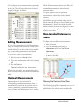
Measurement Table . . . . . . . . . . . . . . . . . . . . 106
Editing Measurements . . . . . . . . . . . . . . . . . . . 107
Optimal Measurements . . . . . . . . . . . . . . . . . . 107
Non-Bonded Distances in Tables . . . . . . . . . . 107
Showing the Deviation from Plane . . . . . . . . . 107
Removing Measurements from a Table . . . . . . 108
Displaying the Coordinates Tables. . . . . . . . . . 108
Internal Coordinates . . . . . . . . . . . . . . . . . . . . 108
Cartesian Coordinates . . . . . . . . . . . . . . . . . . . 109
Comparing Models by Overlay . . . . . . . . . 109
Working With the Model Explorer . . . . . . 111
Model Explorer Objects. . . . . . . . . . . . . . . . . . 112
Creating Groups . . . . . . . . . . . . . . . . . . . . . . . 113
Adding to Groups . . . . . . . . . . . . . . . . . . . . . . 113
Pasting Substructures. . . . . . . . . . . . . . . . . . . . 114
Deleting Groups . . . . . . . . . . . . . . . . . . . . . . . 114
Using the Display Mode . . . . . . . . . . . . . . . . . 114
Coloring Groups . . . . . . . . . . . . . . . . . . . . . . . 114
Resetting Defaults . . . . . . . . . . . . . . . . . . . . . . 115
Animations . . . . . . . . . . . . . . . . . . . . . . . . . . . . 115
Creating and Playing Movies . . . . . . . . . . . . . . 115
Spinning Models . . . . . . . . . . . . . . . . . . . . . . . 115
Spin About Selected Axis. . . . . . . . . . . . . . . . . 115
Editing a Movie. . . . . . . . . . . . . . . . . . . . . . . . . 116
Movie Control Panel. . . . . . . . . . . . . . . . . . . . . 116
Chapter 7: Printing and Exporting Models
Specifying Print Options . . . . . . . . . . . . . . . . . 117
Printing . . . . . . . . . . . . . . . . . . . . . . . . . . . . . . . 118
Exporting Models Using Different File
Formats . . . . . . . . . . . . . . . . . . . . . . . . . . . . . . 118
Publishing Formats. . . . . . . . . . . . . . . . . . . . . . 119
WMF and EMF . . . . . . . . . . . . . . . . . . . . . . . 119
BMP . . . . . . . . . . . . . . . . . . . . . . . . . . . . . . . . 119
EPS . . . . . . . . . . . . . . . . . . . . . . . . . . . . . . . . 120
TIF . . . . . . . . . . . . . . . . . . . . . . . . . . . . . . . . . 120
GIF and PNG and JPG. . . . . . . . . . . . . . . . . . 121
3DM . . . . . . . . . . . . . . . . . . . . . . . . . . . . . . . . 121
AVI . . . . . . . . . . . . . . . . . . . . . . . . . . . . . . . . . 121
Formats for Chemistry Modeling Applications 121
Alchemy . . . . . . . . . . . . . . . . . . . . . . . . . . . . . 121
Cartesian Coordinates . . . . . . . . . . . . . . . . . . . 121
Connection Table . . . . . . . . . . . . . . . . . . . . . . 122
Gaussian Input . . . . . . . . . . . . . . . . . . . . . . . . 122
Gaussian Checkpoint. . . . . . . . . . . . . . . . . . . . 122
Gaussian Cube. . . . . . . . . . . . . . . . . . . . . . . . . 122
Internal Coordinates. . . . . . . . . . . . . . . . . . . . 123
MacroModel Files . . . . . . . . . . . . . . . . . . . . . . 123
Molecular Design Limited MolFile (.MOL) . . . 124
MSI ChemNote . . . . . . . . . . . . . . . . . . . . . . . 124
MOPAC Files. . . . . . . . . . . . . . . . . . . . . . . . . 124
MOPAC Graph Files. . . . . . . . . . . . . . . . . . . . 126
ChemOffice 2005/Chem3D
Protein Data Bank Files . . . . . . . . . . . . . . . . .
ROSDAL Files (RDL) . . . . . . . . . . . . . . . . . .
Standard Molecular Data (SMD) . . . . . . . . . .
SYBYL Files . . . . . . . . . . . . . . . . . . . . . . . . .
126
126
126
126
Job Description File Formats . . . . . . . . . . 126
JDF Files . . . . . . . . . . . . . . . . . . . . . . . . . . . . 126
JDT Files . . . . . . . . . . . . . . . . . . . . . . . . . . . . 126
Exporting With the Clipboard . . . . . . . . . 127
Transferring to ChemDraw . . . . . . . . . . . . . . . 127
Transferring to Other Applications . . . . . . . . . 127
Chapter 8: Computation Concepts
Computational Methods Overview . . . . . 129
Uses of Computational Methods . . . . . . . . . . . 130
Choosing the Best Method. . . . . . . . . . . . . . . . 130
Molecular Mechanics Methods Applications
Summary. . . . . . . . . . . . . . . . . . . . . . . . . . . .
Quantum Mechanical Methods Applications
Summary. . . . . . . . . . . . . . . . . . . . . . . . . . . .
Potential Energy Surfaces . . . . . . . . . . . . . . . .
Potential Energy Surfaces (PES) . . . . . . . . . . .
Single Point Energy Calculations . . . . . . . . . .
Geometry Optimization . . . . . . . . . . . . . . . . .
131
131
132
133
133
134
Molecular Mechanics Theory in Brief . . 135
The Force-Field. . . . . . . . . . . . . . . . . . . . . . . . . 136
MM2 . . . . . . . . . . . . . . . . . . . . . . . . . . . . . . . 136
Bond Stretching Energy . . . . . . . . . . . . . . . . . 137
Angle Bending Energy . . . . . . . . . . . . . . . . . . 137
Torsion Energy. . . . . . . . . . . . . . . . . . . . . . . . 138
Non-Bonded Energy . . . . . . . . . . . . . . . . . . . 139
van der Waals Energy . . . . . . . . . . . . . . . . . . . 139
Cutoff Parameters for van der Waals Interactions 139
Electrostatic Energy . . . . . . . . . . . . . . . . . . . . 140
charge/charge contribution . . . . . . . . . . . . . . 140
dipole/dipole contribution . . . . . . . . . . . . . . . 140
dipole/charge contribution . . . . . . . . . . . . . . . 140
Cutoff Parameters for Electrostatic Interactions 140
OOP Bending. . . . . . . . . . . . . . . . . . . . . . . . . 141
Pi Bonds and Atoms with Pi Bonds . . . . . . . . 141
Stretch-Bend Cross Terms . . . . . . . . . . . . . . . 142
User-Imposed Constraints . . . . . . . . . . . . . . . 142
Molecular Dynamics Simulation . . . . . . . . . . . 142
Molecular Dynamics Formulas . . . . . . . . . . . . 143
Quantum Mechanics Theory in Brief . . 143
Approximations to the Hamiltonian . . . . . . . .
Restrictions on the Wave Function. . . . . . . . .
Spin functions . . . . . . . . . . . . . . . . . . . . . . . .
LCAO and Basis Sets . . . . . . . . . . . . . . . . . .
The Roothaan-Hall Matrix Equation . . . . . . .
Ab Initio vs. Semiempirical. . . . . . . . . . . . . . .
144
145
145
145
146
146
The Semi-empirical Methods . . . . . . . . . . . . . . 146
Extended Hückel Method. . . . . . . . . . . . . . . . 146
•
Methods Available in CS MOPAC . . . . . . . . . 147
RHF . . . . . . . . . . . . . . . . . . . . . . . . . . . . . . . . 147
UHF. . . . . . . . . . . . . . . . . . . . . . . . . . . . . . . . 147
Configuration Interaction . . . . . . . . . . . . . . . . 147
Administrator
Approximate Hamiltonians in MOPAC 148
Choosing a Hamiltonian . . . . . . . . . . . . . . . . . 148
MINDO/3 Applicability and Limitations . . . .
MNDO Applicability and Limitations. . . . . . .
AM1 Applicability and Limitations . . . . . . . . .
PM3 Applicability and Limitations . . . . . . . . .
MNDO-d Applicability and Limitations . . . . .
148
149
149
150
150
Chapter 9: MM2 and MM3 Computations
Minimize Energy . . . . . . . . . . . . . . . . . . . . . . 151
Running a Minimization . . . . . . . . . . . . . . . . .
Queuing Minimizations . . . . . . . . . . . . . . . . . .
Minimizing Ethane . . . . . . . . . . . . . . . . . . . . .
Comparing Two Stable Conformations of
Cyclohexane . . . . . . . . . . . . . . . . . . . . . . . . . .
153
153
154
156
Locating the Global Minimum . . . . . . . . . . . . 157
Molecular Dynamics . . . . . . . . . . . . . . . . . . 158
Performing a Molecular Dynamics Computation 158
Dynamics Settings . . . . . . . . . . . . . . . . . . . . . 158
Job Type Settings . . . . . . . . . . . . . . . . . . . . . . 159
Computing the Molecular Dynamics Trajectory for a
Short Segment of Polytetrafluoroethylene (PTFE) 160
Compute Properties . . . . . . . . . . . . . . . . . . .
Showing Used Parameters . . . . . . . . . . . . .
Repeating an MM2 Computation . . . . . .
Using .jdf Files . . . . . . . . . . . . . . . . . . . . . . . .
161
163
163
163
Chapter 10: MOPAC Computations
MOPAC Semi-empirical Methods . . . . . . 166
Extended Hückel Method . . . . . . . . . . . . . . . .
RHF. . . . . . . . . . . . . . . . . . . . . . . . . . . . . . . . . .
UHF. . . . . . . . . . . . . . . . . . . . . . . . . . . . . . . . . .
Configuration Interaction. . . . . . . . . . . . . . . . .
Approximate Hamiltonians in MOPAC . . . . .
Choosing a Hamiltonian . . . . . . . . . . . . . . . . .
MINDO/3 Applicability and Limitations . . . .
MNDO Applicability and Limitations . . . . . . .
AM1 Applicability and Limitations. . . . . . . . . .
PM3 Applicability and Limitations . . . . . . . . . .
MNDO-d Applicability and Limitations . . . . .
166
166
166
167
167
167
168
168
169
169
170
Using Keywords . . . . . . . . . . . . . . . . . . . . . . . 170
Automatic Keywords . . . . . . . . . . . . . . . . . . . . 170
Additional Keywords . . . . . . . . . . . . . . . . . . . . 171
Specifying the Electronic Configuration 172
Even-Electron Systems . . . . . . . . . . . . . . . . . . 174
Ground State, RHF . . . . . . . . . . . . . . . . . . . . . . 174
Ground State, UHF . . . . . . . . . . . . . . . . . . . . . . 174
•
Excited State, RHF . . . . . . . . . . . . . . . . . . . . . . 174
Excited State, UHF . . . . . . . . . . . . . . . . . . . . . . 175
Odd-Electron Systems. . . . . . . . . . . . . . . . . . . 175
Ground State, RHF . . . . . . . . . . . . . . . . . . . . . . 175
Ground State, UHF. . . . . . . . . . . . . . . . . . . . . . 175
Excited State, RHF . . . . . . . . . . . . . . . . . . . . . . 175
Excited State, UHF . . . . . . . . . . . . . . . . . . . . . . 175
Sparkles. . . . . . . . . . . . . . . . . . . . . . . . . . . . . . . 175
Optimizing Geometry . . . . . . . . . . . . . . . . . . 176
TS. . . . . . . . . . . . . . . . . . . . . . . . . . . . . . . . . . . . 176
BFGS . . . . . . . . . . . . . . . . . . . . . . . . . . . . . . . . . 176
LBFGS . . . . . . . . . . . . . . . . . . . . . . . . . . . . . . . 176
MOPAC Files . . . . . . . . . . . . . . . . . . . . . . . . . . 176
Using the *.out file . . . . . . . . . . . . . . . . . . . . . . 176
Creating an Input File. . . . . . . . . . . . . . . . . . . . 177
Running Input Files . . . . . . . . . . . . . . . . . . . . . 177
Running MOPAC Jobs. . . . . . . . . . . . . . . . . . . 178
Repeating MOPAC Jobs. . . . . . . . . . . . . . . . . . 178
Creating Structures From .arc Files . . . . . . . . . 178
Minimizing Energy . . . . . . . . . . . . . . . . . . . . 180
Notes . . . . . . . . . . . . . . . . . . . . . . . . . . . . . . . . . 181
Adding Keywords . . . . . . . . . . . . . . . . . . . . . . 181
Optimize to Transition State . . . . . . . . . . . 182
Example:. . . . . . . . . . . . . . . . . . . . . . . . . . . . . . 183
Locating the Eclipsed Transition State of Ethane 183
Computing Properties . . . . . . . . . . . . . . . . . 184
MOPAC Properties. . . . . . . . . . . . . . . . . . . . . 185
Heat of Formation, DHf. . . . . . . . . . . . . . . . . . 185
Gradient Norm . . . . . . . . . . . . . . . . . . . . . . . . . 185
Dipole Moment . . . . . . . . . . . . . . . . . . . . . . . . . 186
Charges . . . . . . . . . . . . . . . . . . . . . . . . . . . . . . . 186
Mulliken Charges. . . . . . . . . . . . . . . . . . . . . . . . 186
Charges From an Electrostatic Potential . . . . . 186
Wang-Ford Charges . . . . . . . . . . . . . . . . . . . . . 187
Electrostatic Potential . . . . . . . . . . . . . . . . . . . . 187
Molecular Surfaces . . . . . . . . . . . . . . . . . . . . . . 188
Polarizability . . . . . . . . . . . . . . . . . . . . . . . . . . . 188
COSMO Solvation in Water. . . . . . . . . . . . . . . 188
Hyperfine Coupling Constants . . . . . . . . . . . . . 188
Spin Density . . . . . . . . . . . . . . . . . . . . . . . . . . . 189
Example 1. . . . . . . . . . . . . . . . . . . . . . . . . . . . . 190
The Dipole Moment of Formaldehyde . . . . . . 190
Example 2. . . . . . . . . . . . . . . . . . . . . . . . . . . . . 191
Comparing Cation Stabilities in a Homologous
Series of Molecules . . . . . . . . . . . . . . . . . . . . . 191
Example 3. . . . . . . . . . . . . . . . . . . . . . . . . . . . . 191
Analyzing Charge Distribution in a Series Of
Mono-substituted Phenoxy Ions . . . . . . . . . . 191
Example 4. . . . . . . . . . . . . . . . . . . . . . . . . . . . . 193
Calculating the Dipole Moment of
meta-Nitrotoluene. . . . . . . . . . . . . . . . . . . . . . 193
Example 5. . . . . . . . . . . . . . . . . . . . . . . . . . . . . 194
Comparing the Stability of Glycine Zwitterion
CambridgeSoft
in Water and Gas Phase. . . . . . . . . . . . . . . . . . 194
Example 6 . . . . . . . . . . . . . . . . . . . . . . . . . . . . . 195
Hyperfine Coupling Constants for the Ethyl
Radical . . . . . . . . . . . . . . . . . . . . . . . . . . . . . . . 195
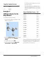
Example 7 . . . . . . . . . . . . . . . . . . . . . . . . . . . . . 196
UHF Spin Density for the Ethyl Radical. . . . . 196
Example 8 . . . . . . . . . . . . . . . . . . . . . . . . . . . . . 197
RHF Spin Density for the Ethyl Radical . . . . . 197
Chapter 11: Gaussian Computations
Gaussian 03 . . . . . . . . . . . . . . . . . . . . . . . . . . . . 199
Minimize Energy . . . . . . . . . . . . . . . . . . . . . . 199
The Job Type Tab . . . . . . . . . . . . . . . . . . . . . . .
The Theory Tab . . . . . . . . . . . . . . . . . . . . . . . .
The Properties Tab . . . . . . . . . . . . . . . . . . . . . .
The General Tab. . . . . . . . . . . . . . . . . . . . . . . .
199
200
201
201
Job Description File Formats . . . . . . . . . . . 202
.jdt Format . . . . . . . . . . . . . . . . . . . . . . . . . . . 202
.jdf Format . . . . . . . . . . . . . . . . . . . . . . . . . . . 202
Computing Properties . . . . . . . . . . . . . . . . . 202
Creating a Gaussian Input File . . . . . . . . . 202
Running a Gaussian Input File . . . . . . . . . 203
Repeating a Gaussian Job . . . . . . . . . . . . . . 204
Running a Gaussian Job . . . . . . . . . . . . . . . 204
Sorting Properties . . . . . . . . . . . . . . . . . . . . . . . 215
Removing Selected Properties . . . . . . . . . . . . . 215
Property Filters. . . . . . . . . . . . . . . . . . . . . . . . 215
Setting Parameters . . . . . . . . . . . . . . . . . . . . 216
Results . . . . . . . . . . . . . . . . . . . . . . . . . . . . . . . . 216
Chapter 15: ChemSAR/Excel
Configuring ChemSAR/Excel . . . . . . . . .
The ChemSAR/Excel Wizard. . . . . . . . . .
Selecting ChemSAR/Excel Descriptors
Adding Calculations to an Existing
Worksheet . . . . . . . . . . . . . . . . . . . . . . . . . . . .
Customizing Calculations . . . . . . . . . . . . .
Calculating Statistical Properties. . . . . . .
217
217
220
220
221
221
Descriptive Statistics . . . . . . . . . . . . . . . . . . . . . 221
Correlation Matrix . . . . . . . . . . . . . . . . . . . . . . 222
Rune Plots . . . . . . . . . . . . . . . . . . . . . . . . . . . . . 222
Appendixes
Accessing the CambridgeSoft Web Site
Chem3D Property Broker . . . . . . . . . . . . . . 205
ChemProp Std Server . . . . . . . . . . . . . . . . . . 205
ChemProp Pro Server . . . . . . . . . . . . . . . . . 207
Registering Online . . . . . . . . . . . . . . . . . . . . 223
Accessing the Online ChemDraw User’s
Guide . . . . . . . . . . . . . . . . . . . . . . . . . . . . . . . . 224
Accessing CambridgeSoft Technical
Support . . . . . . . . . . . . . . . . . . . . . . . . . . . . . . 224
Finding Information on ChemFinder.com 224
Finding Chemical Suppliers on ACX.com 225
Finding ACX Structures and Numbers . 225
MM2 Server . . . . . . . . . . . . . . . . . . . . . . . . . . . 208
MOPAC Server . . . . . . . . . . . . . . . . . . . . . . . . 209
GAMESS Server . . . . . . . . . . . . . . . . . . . . . . . 210
Browsing SciStore.com . . . . . . . . . . . . . . . . 226
Browsing CambridgeSoft.com . . . . . . . . 227
Using the ChemOffice SDK . . . . . . . . . . . 227
Chapter 12: SAR Descriptors
Limitations . . . . . . . . . . . . . . . . . . . . . . . . . . . . 208
Error Messages . . . . . . . . . . . . . . . . . . . . . . . . . 208
Chapter 13: GAMESS Computations
Installing GAMESS . . . . . . . . . . . . . . . . . . . . 211
Minimize Energy . . . . . . . . . . . . . . . . . . . . . . 211
The Theory Tab . . . . . . . . . . . . . . . . . . . . . . . .
The Job Type Tab . . . . . . . . . . . . . . . . . . . . . . .
Specifying Properties to Compute . . . . . . . . . .
Specifying the General Settings . . . . . . . . . . . .
211
212
212
213
Saving Customized Job Descriptions . . . 213
Running a GAMESS Job . . . . . . . . . . . . . . . 213
Repeating a GAMESS Job . . . . . . . . . . . . . . 214
Chapter 14: SAR Descriptor Computations
Selecting Properties To Compute . . . . . . . 215
ChemOffice 2005/Chem3D
ACX Structures . . . . . . . . . . . . . . . . . . . . . . . . . 225
ACX Numbers . . . . . . . . . . . . . . . . . . . . . . . . . 226
Technical Support
Serial Numbers. . . . . . . . . . . . . . . . . . . . . . . . 229
Troubleshooting. . . . . . . . . . . . . . . . . . . . . . . 229
Performance . . . . . . . . . . . . . . . . . . . . . . . . . . . 230
System Crashes . . . . . . . . . . . . . . . . . . . . . . . . . 230
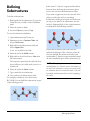
Substructures
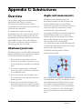
Overview . . . . . . . . . . . . . . . . . . . . . . . . . . . . . . 231
Attachment point rules. . . . . . . . . . . . . . . . . . . 231
Angles and measurements . . . . . . . . . . . . . . . . 231
Defining Substructures . . . . . . . . . . . . . . . . 232
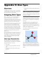
Atom Types
Assigning Atom Types . . . . . . . . . . . . . . . . 233
Atom Type Characteristics . . . . . . . . . . . . . . . . 233
•
Defining Atom Types . . . . . . . . . . . . . . . . . . 234
Keyboard Modifiers
Administrator
Standard Selection . . . . . . . . . . . . . . . . . . . . . 236
Radial Selection . . . . . . . . . . . . . . . . . . . . . . . 236
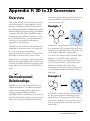
2D to 3D Conversion
Stereochemical Relationships . . . . . . . . . . 239
Example 1
Example 2
Example 3
Example 4
............................
............................
............................
............................
239
239
240
240
Labels. . . . . . . . . . . . . . . . . . . . . . . . . . . . . . . . . 240
File Formats
Editing File Format Atom Types . . . . . . 241
Name . . . . . . . . . . . . . . . . . . . . . . . . . . . . . . . . 241
Description. . . . . . . . . . . . . . . . . . . . . . . . . . . . 241
File Format Examples . . . . . . . . . . . . . . . . . 241
Alchemy File . . . . . . . . . . . . . . . . . . . . . . . . . . 241
FORTRAN Formats . . . . . . . . . . . . . . . . . . . 242
Cartesian Coordinate Files . . . . . . . . . . . . . . . 243
Atom Types in Cartesian Coordinate Files . . . 243
The Cartesian Coordinate File Format . . . . . . 243
FORTRAN Formats . . . . . . . . . . . . . . . . . . . 246
Cambridge Crystal Data Bank Files . . . . . . . . 246
Internal Coordinates File. . . . . . . . . . . . . . . . . 246
Bonds . . . . . . . . . . . . . . . . . . . . . . . . . . . . . . . 248
FORTRAN Formats . . . . . . . . . . . . . . . . . . . 249
MacroModel . . . . . . . . . . . . . . . . . . . . . . . . . . . 249
FORTRAN Formats . . . . . . . . . . . . . . . . . . . 250
MDL MolFile . . . . . . . . . . . . . . . . . . . . . . . . . . 250
Limitations . . . . . . . . . . . . . . . . . . . . . . . . . . . 253
FORTRAN Formats . . . . . . . . . . . . . . . . . . . 253
MSI MolFile . . . . . . . . . . . . . . . . . . . . . . . . . . 253
FORTRAN Formats . . . . . . . . . . . . . . . . . . . 257
MOPAC . . . . . . . . . . . . . . . . . . . . . . . . . . . . . . 257
FORTRAN Formats . . . . . . . . . . . . . . . . . . . 259
Protein Data Bank Files . . . . . . . . . . . . . . . 259
FORTRAN Formats . . . . . . . . . . . . . . . . . . . 260
ROSDAL . . . . . . . . . . . . . . . . . . . . . . . . . . . . . 262
SMD . . . . . . . . . . . . . . . . . . . . . . . . . . . . . . . . . 262
SYBYL MOL File . . . . . . . . . . . . . . . . . . . . . . 265
FORTRAN Formats . . . . . . . . . . . . . . . . . . . 267
SYBYL MOL2 File . . . . . . . . . . . . . . . . . . . . . 267
FORTRAN Formats . . . . . . . . . . . . . . . . . . . 270
Parameter Tables
Parameter Table Use . . . . . . . . . . . . . . . . . . 271
Parameter Table Fields . . . . . . . . . . . . . . . . 272
Atom Type Numbers. . . . . . . . . . . . . . . . . . . . 272
Quality . . . . . . . . . . . . . . . . . . . . . . . . . . . . . . . 273
Reference . . . . . . . . . . . . . . . . . . . . . . . . . . . . . 273
•
Estimating Parameters . . . . . . . . . . . . . . . . . 273
Creating Parameters . . . . . . . . . . . . . . . . . . . 273
The Elements. . . . . . . . . . . . . . . . . . . . . . . . . . 274
Symbol . . . . . . . . . . . . . . . . . . . . . . . . . . . . . . . 274
Covalent Radius . . . . . . . . . . . . . . . . . . . . . . . . 274
Color. . . . . . . . . . . . . . . . . . . . . . . . . . . . . . . . . 274
Atom Types. . . . . . . . . . . . . . . . . . . . . . . . . . . . 274
Name . . . . . . . . . . . . . . . . . . . . . . . . . . . . . . . .
Symbol . . . . . . . . . . . . . . . . . . . . . . . . . . . . . . .
van der Waals Radius . . . . . . . . . . . . . . . . . . . .
Text Number (Atom Type) . . . . . . . . . . . . . . .
Charge. . . . . . . . . . . . . . . . . . . . . . . . . . . . . . . .
Maximum Ring Size . . . . . . . . . . . . . . . . . . . . .
Rectification Type . . . . . . . . . . . . . . . . . . . . . .
Geometry . . . . . . . . . . . . . . . . . . . . . . . . . . . . .
Number of Double Bonds, Triple Bonds, and
Delocalized Bonds . . . . . . . . . . . . . . . . . . . . .
Bound-to Order . . . . . . . . . . . . . . . . . . . . . . . .
Bound-to Type . . . . . . . . . . . . . . . . . . . . . . . . .
274
274
275
275
275
275
275
276
276
276
276
Substructures . . . . . . . . . . . . . . . . . . . . . . . . . . 277
References . . . . . . . . . . . . . . . . . . . . . . . . . . . . . 277
Reference Number. . . . . . . . . . . . . . . . . . . . . . 277
Reference Description . . . . . . . . . . . . . . . . . . . 277
Bond Stretching Parameters . . . . . . . . . . . . 277
Bond Type . . . . . . . . . . . . . . . . . . . . . . . . . . . . 277
KS . . . . . . . . . . . . . . . . . . . . . . . . . . . . . . . . . . . 278
Length. . . . . . . . . . . . . . . . . . . . . . . . . . . . . . . . 278
Bond Dipole. . . . . . . . . . . . . . . . . . . . . . . . . . . 278
Record Order . . . . . . . . . . . . . . . . . . . . . . . . . . 278
Angle Bending, 4-Membered Ring Angle
Bending, 3-Membered Ring Angle
Bending . . . . . . . . . . . . . . . . . . . . . . . . . . . . . . 278
Angle Type . . . . . . . . . . . . . . . . . . . . . . . . . . . .
KB. . . . . . . . . . . . . . . . . . . . . . . . . . . . . . . . . . .
–XR2– . . . . . . . . . . . . . . . . . . . . . . . . . . . . . . .
–XRH– . . . . . . . . . . . . . . . . . . . . . . . . . . . . . . .
–XH2– . . . . . . . . . . . . . . . . . . . . . . . . . . . . . . .
Record Order . . . . . . . . . . . . . . . . . . . . . . . . . .
279
279
279
279
280
280
Pi Atoms . . . . . . . . . . . . . . . . . . . . . . . . . . . . . . 280
Atom Type . . . . . . . . . . . . . . . . . . . . . . . . . . . . 280
Electron . . . . . . . . . . . . . . . . . . . . . . . . . . . . . . 280
Ionization . . . . . . . . . . . . . . . . . . . . . . . . . . . . . 280
Repulsion . . . . . . . . . . . . . . . . . . . . . . . . . . . . . 280
Pi Bonds. . . . . . . . . . . . . . . . . . . . . . . . . . . . . . . 281
Bond Type . . . . . . . . . . . . . . . . . . . . . . . . . . . . 281
dForce. . . . . . . . . . . . . . . . . . . . . . . . . . . . . . . . 281
dLength . . . . . . . . . . . . . . . . . . . . . . . . . . . . . . 281
Record Order . . . . . . . . . . . . . . . . . . . . . . . . . . 281
Electronegativity Adjustments . . . . . . . . . 281
MM2 Constants . . . . . . . . . . . . . . . . . . . . . . . . 282
Cubic and Quartic Stretch Constants . . . . . . . 282
CambridgeSoft
Type 2 (-CHR-) Bending Force Parameters for
C-C-C Angles . . . . . . . . . . . . . . . . . . . . . . . . . 282
Stretch-Bend Parameters . . . . . . . . . . . . . . . . . 283
Sextic Bending Constant . . . . . . . . . . . . . . . . . 283
Dielectric Constants . . . . . . . . . . . . . . . . . . . . . 283
Electrostatic and van der Waals Cutoff
Parameters . . . . . . . . . . . . . . . . . . . . . . . . . . . . 283
MM2 Atom Types . . . . . . . . . . . . . . . . . . . . . 283
Atom type number . . . . . . . . . . . . . . . . . . . . . .
R*. . . . . . . . . . . . . . . . . . . . . . . . . . . . . . . . . . . .
Eps. . . . . . . . . . . . . . . . . . . . . . . . . . . . . . . . . . .
Reduct . . . . . . . . . . . . . . . . . . . . . . . . . . . . . . . .
Atomic Weight . . . . . . . . . . . . . . . . . . . . . . . . .
Lone Pairs . . . . . . . . . . . . . . . . . . . . . . . . . . . . .
Torsional Parameters . . . . . . . . . . . . . . . . . .
Dihedral Type . . . . . . . . . . . . . . . . . . . . . . . . . .
V1 . . . . . . . . . . . . . . . . . . . . . . . . . . . . . . . . . . .
V2 . . . . . . . . . . . . . . . . . . . . . . . . . . . . . . . . . . .
V3 . . . . . . . . . . . . . . . . . . . . . . . . . . . . . . . . . . .
Record Order . . . . . . . . . . . . . . . . . . . . . . . . . .
Out-of-Plane Bending. . . . . . . . . . . . . . . . . .
Bond Type. . . . . . . . . . . . . . . . . . . . . . . . . . . . .
ChemOffice 2005/Chem3D
283
284
284
284
284
284
284
285
285
285
286
287
287
287
Force Constant . . . . . . . . . . . . . . . . . . . . . . . . . 287
Record Order . . . . . . . . . . . . . . . . . . . . . . . . . . 287
VDW Interactions . . . . . . . . . . . . . . . . . . . . 288
Record Order . . . . . . . . . . . . . . . . . . . . . . . . . . 288
MM2
MM2 Parameters . . . . . . . . . . . . . . . . . . . . . . 289
Other Parameters. . . . . . . . . . . . . . . . . . . . . . 289
Viewing Parameters . . . . . . . . . . . . . . . . . . . 289
Editing Parameters . . . . . . . . . . . . . . . . . . . . 290
The MM2 Force Field in Chem3D . . . . . 290
Chem3D Changes to Allinger’s Force Field 290
Charge-Dipole Interaction Term . . . . . . . . . . .
Quartic Stretching Term. . . . . . . . . . . . . . . . . .
Electrostatic and van der Waals Cutoff Terms
Pi Orbital SCF Computation . . . . . . . . . . . . . .
291
291
291
291
MOPAC
MOPAC Background . . . . . . . . . . . . . . . . . . . . 293
Potential Functions Parameters . . . . . . . . 293
Adding Parameters to MOPAC . . . . . . . . 294
•
Administrator
•
CambridgeSoft
Introduction
About Chem3D
Chem3D is an application designed to enable
scientists to model chemicals. It combines powerful
building, analysis, and computational tools with a
easy-to-use graphical user interface, and a powerful
scripting interface.
Chem3D provides computational tools based on
molecular mechanics for optimizing models,
conformational searching, molecular dynamics, and
calculating single point energies for molecules.
About CS MOPAC
CS MOPAC is an implementation of the well
known semi-empirical modeling application
MOPAC, which takes advantage of the easy-to-use
interface of Chem3D. CS MOPAC currently
supports MOPAC 2002.
There are two CS MOPAC options available with
Chem3D 9.0.1:
• MOPAC Ultra
• MOPAC Pro
MOPAC Ultra is the full MOPAC implementation,
and is only available as an optional addin. The CS
MOPAC Ultra implementation provides support
for previously unavailable features such as
MOZYME and PM5 methods.
MOPAC Pro allows you to compute properties,
perform simple (and some advanced) energy
minimizations, optimize to transition states, and
compute properties. The CS MOPAC Pro
implementation supports MOPAC sparkles, has an
improved user interface, and provides faster
calculations. It is included in some versions of
ChemOffice 2005/Chem3D
Chem3D, or may be purchased as an optional
addin. Contact CambridgeSoft sales or your local
reseller for details.
CAUTION
If you have CS MOPAC installed on your computer from
a previous Chem3D or ChemOffice installation,
upgrading to version 9.0.1 will remove your existing
MOPAC installation. See the ReadMe for instructions
on saving your existing MOPAC menu extensions.
See Chapter 10, “MOPAC Computations” on
page 165 for more information on using CS
MOPAC.
About Gaussian
Gaussian is a cluster of programs for performing
semi-empirical and ab initio molecular orbital (MO)
calculations. Gaussian is not included with CS
Chem3D, but is available from SciStore.com,
http://scistore.cambridgesoft.com/software/ .
When Gaussian is correctly installed, Chem3D
communicates with it and serves as a graphical
front end for Gaussian’s text-based input and
output.
Chem3D is compatible with Gaussian 03 for
Windows, and requires the 32-bit version.
About CS Mechanics
CS Mechanics is an add-in module for Chem3D. It
provides three force-fields—MM2, MM3, and
MM3 (Proteins)—and several optimizers that allow
for more controlled molecular mechanics
calculations. The default optimizer used is the
Truncated-Newton-Raphson method, which
Introduction
About CS MOPAC
•
9
provides a balance between speed and accuracy.
Other methods are provided that are either fast and
less accurate, or slow but more accurate.
Administrator
What’s New in
Chem3D 9.0?
Chem3D 9.0 is enhanced by the following features:
What’s New in Chem3D
9.0.1?
• View translation tool—translate (pan) the
•
• Redesigned GUI—User customizable, with
•
•
•
•
•
•
•
new toolbars, new layout for tables and
subviews, new menus and dialogs. The GUI
has been redesigned from the ground up to
make it more usable.
New Model Hierarchy Tree Control—Lets
you open and close fragments, chains, or
groups; change display properties at different
levels. See “Working With the Model Explorer”
on page 111.
ChemDraw panel—Building small molecules
is easier than ever. See “Building with the
ChemDraw Panel” on page 74.
New menu organization—Important
functions are easier to locate.
Full screen mode—Use Chem3D for demos
or instruction.
New Dihedral Driver—Do conformation
analysis with graphical display of results. See
“Tutorial 5: Mapping Conformations with the
Dihedral Driver” on page 42.
Improved support for small molecule
overlays—compare different conformations
or different structures. See “Tutorial 6:
Overlaying Models” on page 43.
XML table editor—easier to use, better
integration.
10 •Introduction
•
•
•
•
•
view without changing the model coordinates.
See “Moving Models with the Translate Tool”
on page 96.
Safer viewing—new “pure selection tool”
prevents unintentionally moving or rotating
parts of the model while selecting. See “The
Building Toolbar” on page 20.
Global keyboard modifiers—advanced users
can perform any action while in any mode
using a global keyboard modifier. See
“Keyboard Modifiers” on page 235.
Improved Zoom control—zoom to center of
screen, center of selection, or center of
rotation. See “Zoom and Translate” on page
235.
Display axes—display or hide axes centered at
the origin of the model, or at the origin of the
view focus.
Middle mouse button and scroll wheel
support—use scroll wheel to zoom, middle
mouse button to rotate or translate. See entries
under “Rotation” and “Zoom and Translate”
on page 235.
New tools for large models:
• View focus—selects a subset of the model
for viewing and manipulation. See “View
Focus” on page 85.
• Select higher group—double click a
selection to select the next higher group. See
“Selecting a Group or Fragment” on page
93.
• Radial Selection—select atoms or groups
within a specified radius. See “Selecting
Atoms or Groups by Distance” on page 94.
CambridgeSoft
What’s New in Chem3D 9.0?
For Users of Previous
Versions of Chem3D
Many features have changed in Chem3D 9.0. Please
note the following:
• The rotation bars are now dynamic rather than
permanently displayed. See “Rotation Bars” on
page 14 for details.
• Internal rotations have changed. See “Rotating
Models” on page 96 for details on how to
perform internal rotations.
• The Measurements table has been augmented
by three other tables: the Model Explorer, the
Cartesian Coordinates table, and the Z-Matrix
table. See “The Model Explorer” on page 27,
and “Model Coordinates” on page 28for more
details.
• Menus and toolbars have changed. Consult the
relevant sections of the manual for details.
CambridgeSoft Web Pages
The following table contains the addresses of
ChemDraw-related web pages.
For
information
about …
Access …
Technical
Support
http://www.cambridgesoft.com/
services
ChemDraw
Plugin
http://products.cambridgesoft.c
om/ProdInfo.cfm?pid=278
http://products.cambridgesoft.c
om/ProdInfo.cfm?pid=279
http://sdk.cambridgesoft.com/
Software
Developer’s kit
ChemOffice 2005/Chem3D
For
information
about …
Access …
ActiveX control http://sdk.cambridgesoft.com/
Purchasing
CambridgeSoft
products and
chemicals
http://chemstore.cambridgesoft.
com/
Installation and
System Requirements
Before installation, see the “ReadMeFirst” and any
other ReadMe documents on the installation CDROM.
Microsoft®Windows®
Requirements
• Windows 2000 or XP.
• Microsoft® Excel add-ins require Office 2000,
2003, or XP.
• ChemDraw plugins/ActiveX® controls
support Netscape® 6.2.x and 7.x, Mozilla 1.x,
and Microsoft IE 5.5 SP2 and 6.x. The
Chem3D ActiveX control supports IE 5.5 SP2
and 6.x only. There is no Chem3D plugin
available.
NOTE: Windows XP Service Pack 2 includes security
features that automatically block active content. This means
that by default, Internet Explorer blocks ChemDraw and
Chem3D ActiveX controls. To activate them, you must
choose the option to "allow blocked content" from the bar
appearing under the address bar notifying you that the
security settings have blocked some of the content of the page.
IE does not remember this information, so you must repeat
Introduction
Installation and System Requirements
•
11
the activation each time you access the page.
If you visit a site frequently, you can add it to the list of
trusted sites in IE’s security settings.
Administrator
• Screen resolution must be 800 x 600 or higher.
Site License Network
Installation Instructions
If you have purchased a site license, please see the
following web site for network installation
instructions:
http://www.cambridgesoft.com/services/sl/
12 •Introduction
CambridgeSoft
Installation and System Requirements
Chapter 1: Chem3D Basics
The Graphical User
Interface
The Graphical User Interface (GUI) is the part of
Chem3D that you interact with to perform tasks.
The GUI consists of a model window, menus,
toolbars and dialog boxes. It can also include up to
three optional panels that display Output and
Building Toolbar
Computation Toolbar
Comments boxes, the Model Explorer and tables
(Cartesian coordinates, Z-Matrix, and
Measurement), and the ChemDraw Panel. At the
bottom of the GUI is a Status bar which displays
information about the active frame of your model
and about hidden atoms in your model. The GUI is
shown in Rotation mode with the dynamic
Rotation bars showing, the ChemDraw panel open,
and the Tables panel set to Auto-Hide.
Model Display Toolbar
ChemDraw Panel
tab
Title bar
Menu bar
Standard
Toolbar
Active
Window
Tab
Model
Explorer tab
Model window
Status bar
Model Window
The Model window is the work space where you do
your modeling. If there is textual information about
ChemOffice 2005/Chem3D
the model, it appears in the Output window or the
Status bar.
Chem3D Basics
The Graphical User Interface
•
13
The following table describes the objects in the
Model window.
Administrator
Object
Description
Model area
The workspace where a
molecular model is viewed, built,
edited, or analyzed. The origin
of the Cartesian axes (0,0,0) is
always located at the center of
this window, regardless of how
the model is moved or scaled.
The Cartesian axes do not move
relative to the window.
Active Window Chem3D 9 can open multiple
tab
models simultaneously. The tab
selects the active window.
Rotation Bars
Chem3D 9 introduces dynamic (auto-hide) rotation
bars. The rotation bars only appear on your screen
when you are actually using them. To view the
dynamic rotation bars you must do two things:
• Activate rotation mode by selecting the
Trackball tool.
• “Mouse over” the rotation bar area.
Z-axis
X-axis
Click on a bar and drag to rotate a model around
that axis. The “Rotate About a Bond” bar is only
active when a bond or dihedral is selected.
Freehand rotation is accomplished by dragging in
the main window. The cursor changes to a hand
when you are in freehand rotation mode.
You can turn off the display (but not the function)
of the bars with the Show Mouse Rotation Zones
checkbox on the GUI tab of the Preferences dialog
box (File > Preferences).
Menus and Toolbars
All Chem3D commands and functions can be
accessed from the menus or toolbars. The toolbars
contain icons that offer shortcuts to many
commonly used functions. You can activate the
Toolbars you want from the Toolbars submenu of
the View menu.
Toolbars can be attached to any side of the GUI, or
can be “torn off ” and placed anywhere on the
screen for convenience.
TIP: Most Toolbar commands are duplicated from the
menus, and are intended as a convenience. If you only use a
command infrequently, you can save clutter by using the menu
commands.
The File Menu
In addition to the usual File commands, you use the
File menu to access the Chem3D Templates and
Preferences, and the Model Settings.
• Import File—Import MOL2 and SD files into
Chem3D a document. The import utility
accurately preserves model coordinates.
• Model Settings—Displays the Settings dialog
Bond axis
14 •Chem3D Basics
Y-axis
box. Set defaults for display modes and colors,
model building, atom and ligand display, atom
labels and fonts, movie and stereo pair settings,
and atom/bond popup label information.
CambridgeSoft
The Graphical User Interface
• Preferences—Displays the Preferences dialog
box. Set defaults for image export, calculation
output path, OpenGL settings and including
hydrogens in CDX format files.
• Sample Files—Accesses example models.
The Edit Menu
In addition to the usual Edit functions, you can use
the Edit menu to copy the model in different
formats, to clear the model window, and to select all
or part of the model.
• Copy as—Puts the model on the Clipboard in
ChemDraw format, as a SMILES string, or in
bitmap format.
• Copy As ChemDraw Structure—Puts the
model on the Clipboard in CDX format. You
may only paste the structure into an application
that can accept this format, for example
ChemDraw, ChemFinder, or Chem3D.
• Copy As SMILES—Puts the model on the
Clipboard as a SMILES string. You may only
paste the structure into an application that can
accept this format.
• Copy As Picture—Puts the model on the
Clipboard as a bitmap. You may only paste the
structure into an application that can accept
bitmaps.
NOTE: The application you paste into must recognize the
format. For example, you cannot paste a ChemDraw
structure into a Microsoft Word document.
• Paste Special—Preserves coordinates when
pasting a Chem3D model from one document
to another.
• Clear—Clears the model window of all
structures.
• Select All—Selects the entire model.
• Select Fragment—If you have selected an
atom, selects the fragment that atom belongs
to.
The View Menu/Model Display Toolbar
Use the View menu to select the view position and
focus, as well as which toolbars, tables, and panels
are visible. The Model Display submenu of the View
menu duplicates all of the commands in the Model
Display toolbar.
• View Position—The View Position submenu
gives you options for centering the view, fitting
the window, and aligning the view with an axis.
• View Focus—The View Focus submenus is
used to set the focus. See “View Focus” on
page 85
• Model Display—Duplicates the Model
Display toolbar—Contains tools to control the
display of the model. These tools are
duplicated on the View menu..
• Show Atom Labels—A toggle switch to
display or hide the atom labels.
• Show Serial Numbers—A toggle switch to
display or hide the atom numbers.
• Show Atom Dots—Displays or hides atom
dot surfaces for the model. The dot surface is
based on VDW radius or Partial Charges, as
set in the Atom Display table of the Settings
dialog box.
• Show Atom Spheres—Displays or hides
atom spheres for the model. The radius is
based on VDW radius or Partial Charges, as
set in the Atom Display table of the Settings
dialog box.
• Show Hs and Lps—A toggle switch to
display or hide hydrogen atoms and lone
pairs.
• Red and Blue glasses—A toggle switch to
set the display for optimal viewing with redblue 3D glasses to create a stereo effect.
ChemOffice 2005/Chem3D
Chem3D Basics
The Graphical User Interface
•
15
Administrator
• Stereo Pairs—A toggle switch to enhance
three dimensional effect by displaying a
model with two slightly different
orientations. It can also create orthogonal
(simultaneous front and side) views. The
degree of separation is set on the Stereo View
tab of the Settings dialog box.
• Perspective—A toggle switch to create a
perspective rendering of the model by
consistent scaling of bond lengths and atom
sizes by depth. The degree of scaling is
controlled by the Perspective “Field of View”
slider on the Model Display tab of the
Settings dialog box.
• Depth Fading—A toggle switch to create a
realistic depth effect, where more distant
parts of the model fade into the background.
The degree of fading is controlled by the
Depth Fading “Field of View” slider on the
Model Display tab of the Settings dialog box.
• Model Axes—Displays or hides the Model
axes.
• View Axes—Displays or hides the view
axes.
NOTE: When both axes overlap and the Model axes
are displayed, the View axes are not visible.
• Background Color—Displays the
Background color select toolbar. Dark
backgrounds are best for viewing protein
ribbon or cartoon displays. Selecting redblue or Chromatek 3D display will
automatically override the background color
to display the optimal black background.
Background colors are not used when
printing, except for Ribbon displays. When
saving a model as a GIF file, the background
will be transparent, if you have selected that
option for Image Export in the Preferences
dialog box.
16 •Chem3D Basics
• Color By—Selects the model coloring
scheme. See “Coloring Displays” on page 58
for more information.
• Toolbars—Click the name of a toolbar to
select it for display. Click again to deselect. You
can attach a toolbar to any side of the GUI by
dragging it to where you want it attached. If
you are using a floating toolbar, you can change
its shape by dragging any of its edges.
• Standard toolbar—Contains standard file,
edit, and print tools. The commands are
duplicated on the File and Edit menus.
• Building toolbar—Contains the Select,
Translate, Rotate, and Zoom tools in
addition to the model building tools—
bonds, text building tool, and eraser. These
tools are not duplicated on any menu. This
toolbar is divided into “safe” and “unsafe”
tools. The four “safe” tools on the left
control only the view – they do not affect
the model in any way. This includes the new
“safe” select tool
and the new translate
tool
. The old select tool
is now
called the Move tool. Although it can also be
used to select, it’s primary use is to move
atoms and fragments.
• Model Display toolbar—Contains tools to
control the display of the model. These tools
are duplicated on the View menu.
• Surfaces toolbar—Contains tools to
calculate and display a molecular surface.
Molecular Surface displays provide
information about entire molecules, as
opposed to the atom and bond information
provided by Structure displays.
• Movies toolbar—Contains tools for the
creation and playback of movies. Chem3D
movies are animations of certain
visualization operations, such as iterations
from a computation. They can be viewed in
CambridgeSoft
The Graphical User Interface
Chem3D, or saved in Windows AVI movie
format. The commands are reproduced on
the Movie menu.
• Measurements Table—Displays the
• Calculation toolbar—Performs MM2
•
•
•
•
minimization from a desktop icon. The
spinning- arrow icon shows when any
calculation is running, and the Stop icon can
be used to stop a calculation before it’s
preset termination.
• Status bar—Displays the Status bar, which
displays information about the active frame
of your model.
• Customize—Displays the Customize
dialog box. Customizing toolbars is a
standard MS Windows operation, and is not
described in Chem3D documentation.
Model Explorer—Displays a hierarchical tree
representation of the model. Most useful when
working with complex molecules such as
proteins, the Model Explorer gives you highly
granular control over the model display.
ChemDraw Panel—Displays the ChemDraw
Panel. Use the ChemDraw Panel to build
molecules quickly and easily with familiar
ChemDraw drawing tools. You can import,
export, edit, or create small molecules quickly
and easily using the ChemDraw ActiveX tools
palette.
Cartesian Table—Displays the Cartesian
Coordinates table. Cartesian Coordinates
describe atomic position in terms of X-, Y-,
and Z-coordinates relative to an arbitrary
origin.
Z-Matrix Table—Displays the internal
coordinates, or Z-Matrix, table. Internal
coordinates are the most commonly used
coordinates for preparing a model for further
computation.
ChemOffice 2005/Chem3D
•
•
•
•
•
•
Measurements table.The Measurements table
displays bond lengths, bond angles, dihedral
angles, and ring closures.
Parameters Tables—Displays a list of
external tables that are used by Chem3D to
construct models, perform computations and
display results.
Output Box—Displays the Output box,
which presents textual information about the
model, iterations, etc.
Comments Box—Displays the Comments
box, a place for user comments that is stored
with the file.
Dihedral Chart—Opens the window
displaying results of Dihedral Driver MM2
computation. See “Tutorial 5: Mapping
Conformations with the Dihedral Driver” on
page 42 for more information.
Status Bar—Displays or hides the Status Bar.
Start Spinning Model Demo—Spins the
model on the Y axis. Use stop calculation
on the Calculations toolbar to stop the demo.
• Full Screen—Activates the full screen display.
The Structure Menu
The Structure menu commands populate the
Measurements table and control movement of the
model.
The Measurements submenu
• Set… Measurements—Sets a
measurement—bond length, angle, or
distance—according to what is selected.
• Bond Lengths—Displays bond lengths in
the Measurements Table. The Actual values
come from the model and the Optimal
values come from the Bond Stretching
Parameters external table.
Chem3D Basics
The Graphical User Interface
•
17
• Bond Angles—Displays bond angles in the
Administrator
Measurements Table. The Actual values
come from the model and the Optimal
values come from Angle Bending
Parameters and other external tables.
• Dihedral Angles—Displays dihedral angles
in the Measurements Table. The Actual
values come from the model and the
Optimal values come from Angle Bending
Parameters and other external tables.
• Clear—Clears the entire Measurement
table. If you only want to clear part of the
table, select the portion you want to clear,
and choose Delete from the right-click
menu.
The Model Position submenu
• Center Model on Origin—Resizes and
•
•
•
•
•
•
•
centers the model in the model window after
a change to the model is made.
Center Selection on Origin—Resizes and
centers the selected portion of the model in
the model window.
Align Model With X Axis—When two
atoms are selected, moves them to the Xaxis.
Align Model With Y-axis—When two
atoms are selected, moves them to the Yaxis.
Align Model With Z-axis—When two
atoms are selected, moves them to the Zaxis.
Align Model With XY Plane—When
three atoms are selected, moves them to the
XY-plane.
Align Model With XZ Plane—When
three atoms are selected, moves them to the
XZ-plane.
Align Model With YZ Plane—When
three atoms are selected, moves them to the
YZ-plane.
18 •Chem3D Basics
The Reflect Model submenu
• Through XY Plane—Reflects the model
through the XY plane by negating Z
coordinates. If the model contains any chiral
centers this will change the model into its
enantiomer. Pro-R positioned atoms will
become Pro-S and Pro-S positioned atoms
will become Pro-R. All dihedral angles used
to position atoms will also be negated.
• Through XZ Plane—Reflects the model
through the XZ plane by negating Y
coordinates. If the model contains any chiral
centers this will change the model into its
enantiomer. Pro-R positioned atoms will
become Pro-S and Pro-S positioned atoms
will become Pro-R. All dihedral angles used
to position atoms will also be negated.
• Through YZ Plane—Reflects the model
through the YZ plane by negating X
coordinates. If the model contains any chiral
centers this will change the model into its
enantiomer. Pro-R positioned atoms will
become Pro-S and Pro-S positioned atoms
will become Pro-R. All dihedral angles used
to position atoms will also be negated.
• Invert Through Origin—Reflects the
model through the origin, negating all
Cartesian coordinates. If the model contains
any chiral centers this will change the model
into its enantiomer. Pro-R positioned atoms
will become Pro-S and Pro-S positioned
atoms will become Pro-R. All dihedral
angles used to position atoms will also be
negated.
The Set Z-Matrix submenu
• Set Origin Atom(s) file—Sets the selected
atom(s) as the origin of the internal
coordinates. Up to three atoms may be
selected. “Setting Measurements” on page
85
CambridgeSoft
The Graphical User Interface
•
•
•
•
•
•
• Position by Dihedrals—Positions an atom
• Overlay—The Overlay submenu provides all
relative to three previously positioned atoms
using a bond distance, a bond angle, and a
dihedral angle. For more information on
changing the internal coordinates see
“Setting Dihedral Angles” on page 86.
• Position by Bond Angles—Positions an
atom relative to three previously positioned
atoms using a bond distance and two bond
angles. For more information on changing
the internal coordinates see “Setting Bond
Angles” on page 86.
Detect Stereochemistry—Scans the model
and lists the stereocenters in the Output box.
Invert—Inverts the isomeric form. For
example, to invert a model from the cis- form
to the trans- form, select one of the stereo
centers and use the Invert command.
Deviation from Plane—When you select four
or more atoms, outputs the RMS deviation
from the plane to the Output window.
Add Centroid—Adds a centroid to a selected
model or fragment. At least two atoms must be
selected. The centroid and “bonds” to the
selected atoms are displayed, and “bond”
lengths can be viewed in the tool tips. To delete
a centroid, select it and press the Delete or
Backspace key.
Rectify—Fills the open valences for an atom,
usually with hydrogen atoms. This command is
only useful if the default automatic rectification
is turned off in the Model Settings dialog box.
Clean Up—Corrects unrealistic bond lengths
and bond angles that may occur when building
models, especially when you build strained ring
systems.
of the commands to enable you to compare
fragments by superimposing one fragment in a
model window over a second fragment. Two
types of overlay are possible: quick, and
minimization. See “Tutorial 6: Overlaying
Models” on page 43, and “Comparing Models
by Overlay” on page 109 for information on
each overlay type.
• Dock—The Dock command enables you to
position a fragment into a desired orientation
and proximity relative to a second fragment.
Each fragment remains rigid during the
docking computation.
ChemOffice 2005/Chem3D
The Standard Toolbar
The Standard toolbar contains tools for standard
Windows functions, including up to 20 steps of
Undo and Redo.
New File
Open File
Save File
Copy
Cut
Paste
Undo
Redo
Print
About Chem3D
Chem3D Basics
The Graphical User Interface
•
19
The Building Toolbar
Administrator
The Building toolbar contains tools that allow you
to create and manipulate models. The tools are
shown below.
For detailed descriptions of the tools see “Building
With the Bond Tools” on page 75, “Rotating
Models” on page 96, and “Resizing Models” on
page 100.
The Model Display Toolbar
“Safe” Select tool (view only)
Translate tool
Trackball tool
Rotation Dial activator
The Model Display toolbar contains tools for all of
the Chem3D display functions. The Model type and
Background color tools activate menus that let you
choose one of the options. All of the remaining
tools are toggle switches—click once to activate;
click again to deactivate.
Zoom tool
Model type
Move tool
Single Bond tool
Background Color
Double Bond tool
Stereo Visualization
Triple Bond tool
Red-Blue Stereo
Uncoordinated Bond tool
Chromatek Stereo
Text tool
Perspective
Eraser tool
The Rotation Dial, activated by clicking the arrow
under the Trackball tool, lets you rotate a model an
exact amount. Select an axis, then drag the dial or
type a number into the box.
Depth Fading
Model Axes
View Axes
Atom labels
Atom numbers
Full screen mode
Spinning model demo
20 •Chem3D Basics
CambridgeSoft
The Graphical User Interface
The Surfaces Toolbar
The Surfaces toolbar controls the display of
molecular surfaces. In most cases, you will need to
do either an Extended Hückel, MOPAC, or
Gaussian calculation before you can display
surfaces.
Surface
For more information on Surfaces, see “Molecular
Surface Displays” on page 63.
The Movie Toolbar
The Movie toolbar controls the creation and
playback of animations. You can animate certain
visualization operations, such as iterations from a
computation, by saving frames in a movie. Movies
can be saved as Windows AVI video files.
Play
Solvent radius
Stop
Display mode
First frame
Color Mapping
Surface color
Resolution
Previous Frame
Position
Next frame
Last frame
HOMO/LUMO selection
Isovalues
Delete
Delete all
Properties
Color A
Color B
ChemOffice 2005/Chem3D
For more information on Movies, see “Creating
and Playing Movies” on page 115.
Chem3D Basics
The Graphical User Interface
•
21
The Calculation Toolbar
Administrator
The Calculation toolbar provides a desktop icon for
performing the most common calculation, MM2
minimization. It also provides a Stop button and a
“calculation running” indicator that work with all
calculations.
Close panel
Auto-Hide
Synchronize
Draw > 3D add
Draw>3D
replace
3D>Draw
Calculation indicator
MM2 minimization
Clean up
structure
Clear
Lock
Stop button
Name=Struct
The ChemDraw Panel
Chem3D 9 makes it easier than ever to create or
edit models in ChemDraw. The ChemDraw panel
is activated from the View menu. By default it opens
on the right side of the GUI, but like the toolbars
you can have it “float” or attach it anywhere you
like.
ChemDraw
ActiveX tool
palette
Use the 3D > Draw icon to drag a Chem3D model
into the ChemDraw panel.
To create a model in ChemDraw, click in the
ChemDraw panel to activate the ChemDraw
toolbar. Use the Draw>3D Add or Draw>3D Replace
icons to put the model in Chem3D—or select the
Synchronize icon to draw in both simultaneously.
You can also create a model by typing the name of
a compound—or a SMILES string—into the
Name=Struct™ box. When you finish editing, add
or replace your Chem3D model by clicking the
appropriate icon.
22 •Chem3D Basics
CambridgeSoft
The Graphical User Interface
The Model Information
Panel
The following table describes the elements of the
Measurement table.
The Model information panel contains information
about the model in the top-most tabbed window
and its display. You can display one or more of the
following tables in the area:
Table Element
Description
Column Heading
Contains field names
describing the information in
the table.
Record Selector
Used to select an entire
record. Clicking a record
selector highlights the
corresponding atoms in the
model window.
Field Name
Identifies the type of
information in the cells with
which it is associated.
Column Divider
Used to change the width of
the column by dragging.
Cell
Contains one value of one
field in a record. All records
in a given table contain the
same number of cells.
• Model Explorer
• Measurements
• Cartesian Coordinates
• Z-Matrix table
Tables are linked to the structure so that selecting
an atom, bond, or angle in either will highlight both.
Numerical values in the tables can be edited or cut
and pasted to/from other documents (text or Excel
worksheets), and the changes are displayed in the
structure.
All of the tables have an Auto-hide feature to
minimize their display. For more information on
Model Tables, see “Model Coordinates” on page
28.
The Z-Matrix table is shown below:
Field Name
Column
Record
Heading
Selector
Column Divider
Cell
The Output and Comments
Windows
The Output and Comments boxes are typically
found at the bottom of the GUI window. You can
have them float if you wish, or move them to
another side of the window. You can select Autohide to minimize them.
Calculations on models and other operations
produce messages that are displayed in the Output
window.You can save the information in the
Output window either directly or using the
clipboard. To save information directly:
ChemOffice 2005/Chem3D
Chem3D Basics
The Graphical User Interface
•
23
1. Right-click in the window and choose Export.
Administrator
A Save As dialog box appears.
2. Enter a name for the file, select a file format
(.html or .txt) and click Save.
To save information with the clipboard:
1. Select the text you want to save.
2. Right-click in the window and choose Copy.
Alternately, you can choose Select All from the
right-click menu.
3. Paste into the document of your choice.
You must use Copy – Paste to restore information
from a saved file.
You can remove information from the Output
window without affecting the model.
To remove messages:
1. Select the text you want to delete.
2. Do one of the following:
• From the Right-click menu, choose Clear.
• Press the Delete or Backspace key.
The Comments window gives you a place to add
notes and comments about the model. When you
save a model, comments are also saved.
Model Building Basics
As you create models, Chem3D applies standard
parameters from external tables along with userselected settings to produce the model display.
There are several options for selecting your desired
display settings: you can change defaults in the
Model Settings dialog box, use menu or toolbar
commands, or use context-sensitive menus (rightclick menus) in the Model Explorer. You can also
view and change model coordinates.
24 •Chem3D Basics
Internal and External Tables
Chem3D uses two types of parameter tables:
• Internal tables—Contain information about a
specific model.
Examples of internal tables are:
• Measurements table
• Z-Matrix table
• Internal coordinates table
• External tables—Contain information used
by all models.
Examples of external tables are:
• Elements, Atom Types, and Substructures
tables that you use to build models.
• Torsional Parameters tables that are used by
Chem3D when you perform an MM2
computation.
• Tables that store data gathered during
Dihedral Driver conformational searches.
Standard Measurements—Standard
measurements are the optimal (or equilibrium)
bond lengths and angles between atoms based on
their atom type. The values for each particular atom
type combination are actually an average for many
compounds each of which have that atom type (for
example, a family of alkanes). Standard
measurements allow you to build models whose 3D
representation is a fair approximation of the actual
geometry when other forces and interactions
between atoms are not considered.
For more information on External Tables, see
“Parameter Tables” on page 271.
To view an internal table:
• Choose the table from the View menu.
CambridgeSoft
Model Building Basics
To view an external table:
• Point to Parameter Tables on the View menu,
then choose the table to view.
The settings are organized into tabbed panels. To
select a control panel, click one of the tabs at the
top of the dialog box.
TIP: You can superimpose multiple tables if you
Model Display
attach them to an edge of the GUI. One table will be
visible and the others will display as selection tabs.
Attached tables have the Auto-hide feature.
The model of ethane shown below displays the
cylindrical bonds display type (rendering type) with
the element symbols and serial numbers for all
atoms.
To auto-hide a table:
• Push the pin in the upper right corner of the
table.
The table minimizes to a tab when you are not
using it.
Atom serial numbers
Element symbols
The Model Setting Dialog
Box
The Chem3D Model Settings dialog box allows you
to configure settings for your model.
To open the Chem3D Model Settings dialog box:
• From the File menu, choose Model Settings.
The Settings dialog box appears:
To specify the rendering type do one of the
following:
• From the View menu, point to Model Display,
then Display Mode, and select a rendering type.
• Activate the Model Display toolbar, click the
arrow next to the Model Display icon
,
and select a rendering type.
• In the Model Settings dialog box, choose
Model Display, and select a rendering type.
To specify the display of serial numbers and
element symbols, do one of the following:
• On the View menu, point to Model Display,
then click Show Serial Number or Show Atom
Label.
• Activate the Model Display toolbar and click
the Atom Labels and Serial Numbers icons.
ChemOffice 2005/Chem3D
Chem3D Basics
Model Building Basics
•
25
• In the Model Settings dialog box, select the
Administrator
Atom Labels tab, and check the box next to
Show Element Symbols and Show Serial
Numbers.
The following illustration shows the model label for
the bond between C(1) and C(2).
The serial number for each atom is assigned in the
order of building. However, you can reserialize the
atoms. For more information see “Setting Serial
Numbers” on page 88.
The element symbol comes from the Elements
table. The default color used for an element is also
defined in the Elements table. For more
information, see “Coloring by Element” on page 58
and “The Elements” on page 274.
Model Data Labels
When you point to an atom, information about the
atom appears in a model label pop-up window. By
default, this information includes the element
symbol, serial number, atom type, and formal
charge.
The following illustration shows the model label for
the C(1) atom of ethane.
The model data changes to reflect the atoms that
are selected in the model. For example, when three
contiguous atoms H(3)-C(1)-C(2) are selected, the
model label includes the atom you point to and its
atom type, the other atoms in the selection, and the
angle.
This is shown in the following illustration.
these atoms are selected
they are displayed in yellow
in Chem3D
The model data changes when you point to a bond
instead of an atom.
26 •Chem3D Basics
CambridgeSoft
Model Building Basics
If you select four contiguous atoms the dihedral
angle appears in the model label. If you select two
bonded or non-bonded atoms, the distance
between those atoms appears.
To specify what information appears in atom,
bond, and angle labels:
• In the Model Settings dialog box, select the
Pop-up Info tab, then select the information you
want to display.
Atom Types
Atom types contain much of the Chem3D chemical
intelligence for building models with reasonable 3D
geometries. If an atom type is assigned to an atom,
you can see it in the model data when you point to
it. In the previous illustration of pointing
information, the selected atom has an atom type of
“C Alkane”.
An atom that has an atom type assigned has a
defined geometry, bond orders, type of atom used
to fill open valences (rectification), and standard
bond length and bond angle measurements
(depending on the other atoms making up the
bond).
The easiest way to build models uses a dynamic
assignment of atom types that occurs as you build.
For example, when you change a single bond in a
model of ethane to a double bond, the atom type is
automatically changed from C Alkane to C Alkene.
In the process, the geometry of the carbon and the
number of hydrogens filling open valences changes.
You can also build models without assigning atom
types. This is often quicker, but certain tasks, such
as rectification or MM2 Energy Minimization, will
also correct atom types because atom types are
required to complete these tasks.
To assign atom types as you build:
• In the Chem3D Model Settings dialog box,
select the Model Build tab, then check the
Correct Atom Types checkbox.
ChemOffice 2005/Chem3D
To assign atom types after building:
• Select the atom(s) and use the Rectify command
on the Structure menu.
Atom type information is stored in the Atom Types
table. To view the Atom Types table:
• From the View menu, select Parameter Tables,
then select atom types.xml.
Rectification
Rectification is the process of filling open valences
of the atoms in your model, typically by adding
hydrogen atoms.
To rectify automatically as you build, do the
following:
• In the Chem3D Model Settings dialog box,
select the Model Build tab, and then check the
Rectify checkbox.
If you activate automatic rectification in the Model
Settings dialog box, you have the option of showing
or hiding hydrogens. If you turn off automatic
rectification, the Show Hs and Lps command on the
Model Display submenu of the View menu is
deactivated, and you will not have the option of
displaying hydrogens.
Bond Lengths and Bond Angles
You can apply standard measurements (bond
lengths and bond angles) automatically as you build
or apply them later . Standard measurements are
determined using the atom types for pairs of
bonded atoms or sets of three adjacent atoms, and
are found in the external tables Bond Stretching
Parameters.xml and Angle Bending Parameters.xml.
The Model Explorer
The Model Explorer allows users to explore the
hierarchical nature of a macromolecule and alter
properties at any level in the hierarchy. Display
Chem3D Basics
Model Building Basics
•
27
modes and color settings are easy to control at a
fine-grained level. Properties of atoms and bonds
are easy to access and change.
Administrator
The Model Explorer is designed as a hierarchical
tree control that can be expanded/collapsed as
necessary to view whatever part of the model you
wish. Changes are applied in a bottom-up manner,
so that changes to atoms and bonds override
changes at the chain or fragment level. You can
show/hide/highlight features at any level. Hidden
or changed features are marked in the hierarchical
tree with colored icons, so you can easily keep track
of your edits. See “Working With the Model
Explorer” on page 111 for more information.
Model Coordinates
Each of the atoms in your model occupies a
position in space. In most modeling applications,
there are two ways of representing the position of
each atom: internal coordinates and Cartesian
coordinates. Chem3D establishes internal and
Cartesian coordinates as you build a model.
Z-matrix
Internal coordinates for a model are often referred
to as a Z-matrix (although not strictly correct), and
are the most commonly used coordinates for
preparing a model for further computation.
Changing a Z-matrix allows you to enter relations
between atoms by specifying angles and lengths.
You display the Z-Matrix table by selecting it from
the View menu. You can edit the values within the
table, or move atoms within the model and use the
Set Z-matrix submenu of the Structure menu. You
can copy and paste tables to text (.txt) files or Excel
spreadsheets using the commands in the context
(right-click) menu.
28 •Chem3D Basics
Below is an example of the internal coordinates
(Z-matrix) for ethane:
Cartesian Coordinates
Cartesian coordinates are also commonly accepted
as input to other computation packages. They
describe atomic position in terms of X-, Y-, and
Z-coordinates relative to an arbitrary origin. Often,
the origin corresponds to the first atom drawn.
However, you can set the origin using commands in
the Model Position submenu of the Structure menu.
Instead of editing the coordinates directly in this
table, you can save the model using the Cartesian
Coordinates file format (.cc1 or .cc2), and then edit
that file with a text editor. You can also copy and
paste the table into a text file or Excel worksheet
using the commands in the context (right-click)
menu.
NOTE: If you do edit coordinates in the table, remember to
turn off Rectify and Apply Standard Measurements in
the Model Build panel of the Model Settings dialog while
you edit so that other atoms are not affected.
An example of the Cartesian coordinates for ethane
is shown below.
CambridgeSoft
Model Building Basics
The Measurements Table
The Measurements table displays bond lengths,
bond angles, dihedral angles, and ring closures.
When you first open a Measurements Table, it will
be blank.
If you edit the Actual field, you change the value in
the model, and see atoms in the model move.
If you edit the Optimal value, you apply a constraint.
These values are used only in Clean Up (on the
Structure menu) and MM2 computations.
To display data in a Measurements Table:
• From the Structure menu, point to
Measurements, then select the information you
wish to display.
The example shows the display of Bond Lengths
and Bond Angles for ethane:
Deleting Measurement Table Data
You can isolate the information you in the
Measurements table by deleting the records that
you do not want to view. For example, you could
display bond lengths, then delete everything except
the carbon-carbon bonds. This would make them
easier to compare.
To delete records:
• Select the records and click Delete on the right-
click menu.
Deleting records in a Measurements table does
not delete the corresponding atoms.
To clear the entire table:
• On the Measurement submenu of the Structure
menu, select Clear.
ChemOffice 2005/Chem3D
Chem3D Basics
Model Building Basics
•
29
Administrator
30 •Chem3D Basics
CambridgeSoft
Model Building Basics
Chapter 2: Chem3D Tutorials
Overview
The following section gives detailed examples of
some general tasks you can perform with Chem3D.
For examples of MOPAC calculations, see Chapter
10, “MOPAC Computations” on page 165.
In this section:
• Tutorial 1: Working with ChemDraw on page
31.
• Tutorial 2: Building Models with the Bond
Tools on page 32.
• Tutorial 3: Building Models with the Text
Building Tool on page 36.
• Tutorial 4: Examining Conformations on page
39.
• Tutorial 5: Mapping Conformations with the
Dihedral Driver on page 42.
• Tutorial 6: Overlaying Models on page 43.
• Tutorial 7: Docking Models on page 46.
• Tutorial 8: Viewing Molecular Surfaces on page
48.
• Tutorial 9: Mapping Properties onto Surfaces
on page 49.
• Tutorial 10: Computing Partial Charges on
page 52.
Tutorial 1: Working
with ChemDraw
The following tutorial introduces model building
with Chem3D. It assumes that no defaults have
been changed since installation. If what you see is
not like the description, you may need to reset the
defaults. To reset defaults:
ChemOffice 2005/Chem3D
• From the File menu, open the Model Settings
dialog box. Click the Reset button.
Open a new model window if one is not already
opened. To view models as shown in this tutorial,
select Cylindrical Bonds from the drop-down menu
of the Model Display mode tool on the Model
Display toolbar.
The installation default for the ChemDraw panel is
activated, hidden. You should see a tab labeled
ChemDraw on the upper right side of the GUI.
ChemDraw tab
If you do not see the tab:
1. From the View menu, select ChemDraw Panel.
The ChemDraw Panel opens in its default
position, attached to the right edge of the
model window.
If the tab is visible:
Chem3D Tutorials
Tutorial 1: Working with ChemDraw
•
31
2. Click the ChemDraw tab to open the panel.
TIP: The panel default is Auto-hide. If you want the
panel to stay open, push the pin on the upper right.
Administrator
pin
3. Click in the ChemDraw panel it.
A blue line appears around the ChemDraw
Panel model window, and the ChemDraw
tools palette appears.
4. On the ChemDraw tools palette, select the
Benzene Ring tool.
5. Click in the panel to place a benzene ring.
The ChemDraw structure is converted into a
3D representation.
You can turn off the hot linking by clicking the
Synchronize button. If you do this, you will need to
use the 3D>Draw and Draw>3D buttons to copy
models between the windows.
Synchronize
Draw>3D replace
Cleanup
Draw>3D add 3D>draw
Name=Struct
text box
Clear Lock
TIP: Use Ctrl+A to select the model you want to copy.
Tutorial 2: Building
Models with the Bond
Tools
Draw ethane using a bond tool.
1. Click the Single Bond tool
.
2. Point in the model window, drag to the right
and release the mouse button.
A model of ethane appears. When you rotate
the model in a later step, you will see the other
hydrogen.
You can work with the model in Chem3D. The 2D
and 3D models are hot-linked, so any change in one
changes the other:
1. Double-click one of the hydrogens in the 3D
model.
A text box appears.
2. Type OH in the text box, then hit the Enter key.
3. A phenol molecule is displayed in both the
Chem3D model window and the ChemDraw
window.
32 •Chem3D Tutorials
NOTE: If you are using default settings, hydrogens
are displayed automatically.
To see the three-dimensionality of your model you
can perform rotations using the Trackball tool. The
Trackball Tool mimics a sphere in which your
CambridgeSoft
Tutorial 2: Building Models with the Bond Tools
model is centered. You can rotate your model by
rotating the sphere. You have a choice of free-hand
rotation, or rotating around the X, Y, or Z axis.
3. Release the mouse button when the model is
orientated approximately like this:
To perform free-hand rotation of the model with
the Trackball tool:
1. Click the Trackball tool
.
2. Point near the center of the model window and
hold down the mouse button.
3. Drag the cursor in any direction to rotate the
model.
CAUTION
Users familiar with earlier versions of Chem3D should be
aware of changed behavior: the Trackball tool rotates the
view only, it does not change the atoms’ Cartesian
coordinates.
To rotate around an axis:
1. Move the cursor to the edge of the model
window.
As you mouse over the edge of the window, the
rotation bars will appear.
Examine the atoms and bonds in the model using
the Select tool.
1. Click the Select tool
.
2. Move the pointer over the far left carbon.
NOTE: Depending on how much you rotated the
model, the far left carbon might be C(2).
An information box appears next to the atom
you are pointing at. The first line contains the
atom label. In this case, you are pointing to
C(1). The second line contains the name of the
atom type, C Alkane.
NOTE: Rotation bars are only available when you
are using the Trackball tool.
2. Drag on one of the bars to rotate the model on
that axis.
One of the bars is labeled “Rotate About Bond”.
You won’t be able to select that one. You’ll
cover rotating around bonds later.
TIP: Once you start dragging, you don’t have to stay
within the rotation bar’s boundaries. Your model will
only rotate around the chosen axis no matter where you
drag your mouse.
ChemOffice 2005/Chem3D
Chem3D Tutorials
Tutorial 2: Building Models with the Bond Tools
•
33
3. Move the pointer over the C-C bond to display
its bond length and bond order.
The dihedral angle formed by those four atoms
is displayed.
Administrator
To display information about angles, select several
atoms.
1. Click C(1), then Shift+click C(2) and H(7).
2. Point at any of the selected atoms or bonds.
The angle for the selection appears.
Change the ethane model to an ethylene model.
1. Click the Double Bond tool
.
2. Drag the mouse from C(1) to C(2).
3. Point to the bond.
The bond length decreases and the bond order
increases.
To display information about contiguous atoms:
1. Hold the Shift key and select four contiguous
atoms.
2. Point at any portion of the selection.
Continue to build on this model to build
cyclohexane.
1. Click the Select tool
.
2. Click the double bond.
3. Right click, point to Bond(s), then to Order, and
choose Single Bond.
The bond order is reduced by one.
Hide the hydrogens to make it easier to build.
34 •Chem3D Tutorials
CambridgeSoft
Tutorial 2: Building Models with the Bond Tools
• On the Model Display submenu of the View
menu, deselect Show Hs and Lps.
The hydrogens are hidden.
Add more atoms to the model:
1. Click the Single Bond tool
.
2. Drag upward from the left carbon.
3. Another C-C bond appears.
4. Continue adding bonds until you have 6
carbons as shown below.
ChemOffice 2005/Chem3D
Create a ring:
1. Drag from one terminal carbon across to the
other.
The pointing information appears when you
drag properly.
2. Release the mouse button to close the ring.
Chem3D Tutorials
Tutorial 2: Building Models with the Bond Tools
•
35
Add serial numbers and atom labels.
Administrator
1. On the Model Display submenu of the View
menu, select Show Serial Numbers, or click the
Serial Number icon
on the Model Display
toolbar.
2. On the Model Display submenu of the View
menu, select Show Atom Labels, or click the
Atom Label icon
on the Model Display
toolbar.
NOTE: The serial numbers that appear do not reflect
a normal ordering because you started with a smaller
model and built up from it.
Because you built the structure by using bond tools,
you may have distorted bond angles and bond
lengths.
To correct for distorted angles and lengths:
1. From the Edit menu, choose Select All.
All of the atoms in the model are selected.
2. From the Structure menu, choose Clean Up
Structure.
To locate an energy minimum for your structure
which represents a stable conformation of your
model, click the MM2 Minimize Energy tool
on the Calculation toolbar.
You can reserialize the atoms as follows:
1. Select the Text Building tool
2. Click the first atom.
A text box appears on the atom.
.
3. Type the number you want to assign to this
atom (1 for this example).
4. Press the Enter key.
The first atom is renumbered as (1).
5. Double-click each of the atoms in the order
you want them to be numbered.
Each time you double-click an atom to serialize
it, the new serial number is one greater than the
serial number of the previously serialized atom.
6. From the Model Display submenu of the View
menu, choose Show Hs and Lps and examine
the model using the Trackball Tool
.
The hydrogens appear as far apart as possible.
36 •Chem3D Tutorials
For more information about MM2 and energy
minimization see MM2 on page 136.
After the minimization is complete:
1. From the File menu, choose Save.
2. Select a directory in which to save the file.
3. Type tut1 in the text box at the bottom of the
dialog box.
4. Click Save.
5. Click the model window to activate it.
6. From the File menu, choose Close Window.
Tutorial 3: Building
Models with the Text
Building Tool
This tutorial illustrates alternative methods to build
models using the Text Building Tool. You will start
by opening the file you saved in the first tutorial:
1. From the File menu, choose Open.
2. Locate and select the file, tut1, that you created
in the previous tutorial.
3. Click Open.
CambridgeSoft
Tutorial 3: Building Models with the Text Building Tool
Replacing Atoms
To change one element into another:
1. Click the Text Building tool
.
2. Click a hydrogen atom attached to C(1).
A text box appears.
3. Type C.
NOTE: Element symbols and substructure names are
case sensitive. You must type an uppercase C to create a
carbon atom.
4. Press the Enter key.
The hydrogen attached to C(1) is changed to a
carbon. The valence is filled with hydrogens to
form a methyl group because Automatic
Rectification is turned on.
You don’t have to select the Text tool in order to
use it. Double-clicking with any other tool selected
has the same effect as single-clicking with the Text
tool. To demonstrate this, let’s replace two more
hydrogens using an alternative method:
1. Select the Trackball tool
so that you can
rotate your model to get a better view of what
you are building.
2. Double-click two more hydrogens to change
them to methyl groups.
TIP: Notice that the “C” you entered previously in the Text
tool remains as the default until you change it. You only have
to double-click, and press the Enter key.
Now, refine the structure to an energy minimum to
take into account the additional interactions
imposed by the methyl groups by clicking the MM2
tool
on the Calculation toolbar.
When the minimization is complete:
3. Select a directory in which to save the file.
4. Click Save.
Save a copy of the model using a different name:
1. From the File menu, choose Save As.
2. Type tut2b.
3. Select a directory in which to save the file.
4. Click Save.
We’ll be using these two copies of your model in
later tutorials.
Using Labels to Create
Models
You can also create models by typing atom labels
(element symbols and numbers) into a text box.
CH3
H3C
C
H
H2
C
H
C
CH3
OH
To build the model of 4-methyl-2-pentanol shown
above:
1. From the File menu, choose New, or click the
new file tool on the Standard toolbar.
.
2. Click the Text Building tool
3. Click in the empty space in the model window.
A text box appears where you clicked.
4. In the text box, type
CH3CH(CH3)CH2CH(OH)CH3.
You type labels as if you were naming the
structure: pick the longest chain of carbons as
the backbone, and specify other groups as
substituents. Enclose substituents in
parentheses after the atom to which they are
attached.
1. From the File menu, choose Save As.
2. Type tut2a.
ChemOffice 2005/Chem3D
Chem3D Tutorials
Tutorial 3: Building Models with the Text Building Tool
•
37
6. Select the model and choose Clean Up from the
Structure menu.
5. Press the Enter key.
Administrator
TIP: The Text building tool will also accept structures in
SMILES notation, either typed in or cut and pasted from
other documents.
Another, simpler, way of building this model is to
type Pentane in the Name=Struct text box and then
modify the appropriate hydrogens.
Refine the model as follows.
TIP: You don’t have to click the Select tool every time
you want to select something. Just hold down the letter S
on your keyboard while working with any building tool,
and you temporarily activate the Select tool.
You cannot specify stereochemistry when you build
models with labels. The structure of 1,2-dimethyl
cyclopentane appears in the trans conformation.
1. Click the Select tool
2. Select the model by dragging diagonally across
it.
3. From the Structure menu, choose Clean Up.
If you want a more accurate representation of a low
energy conformation, optimize the geometry of the
model by clicking the MM2 tool
on the
Calculation toolbar.
To obtain the cis-isomer:
To specify text equivalent to the structure of
1,2-dimethyl cyclopentane shown below:
Using Substructures
H2
C
CH2
H 2C
CH
H 3C
1.
2.
3.
4.
5.
CH
CH3
From the File menu, choose New.
Click the Text Building tool
.
Click in the empty space in the model window.
Type CH(CH3)CH(CH3)CH2CH2CH2.
Press the Enter key.
The trans-isomer appears.
1. Click the Select tool
.
2. Select C(1).
3. From the Structure menu, choose Invert.
The cis-isomer appears. You can rotate the
molecule to see the differences between the
isomers after you invert the molecule.
Labels are useful to build simple structures.
However, if you make larger, more complex
structures, you will find it easier to use a
combination of labels and pre-defined
substructures.
Over 200 substructures are pre-defined in
Chem3D. These substructures include the most
commonly used organic structures.
TIP: Pre-defined substructures are listed in the
substructures.xml file. You can view the list by pointing to
Parameter Tables on the View menu and selecting
Substructures. Text typed in the text box is case sensitive.
You must type it exactly as it appears in the Substructures
table.
Build a model of nitrobenzene:
1. From the File menu, choose New.
2. Click the Text Building tool
.
3. Click the empty space in the model window.
38 •Chem3D Tutorials
CambridgeSoft
Tutorial 3: Building Models with the Text Building Tool
4. Type Ph(NO2) in the text box.
5. Press the Enter key.
A model of nitrobenzene appears.
The substructure in this example is the phenyl
group. Substructures are defined with specific
attachment points for other substituents. For
phenyl, the attachment point is C(1).
3. Select the Trackball tool
, and rotate the
model so you are viewing it down the center of
the helix as shown below:
Build a peptide model:
1. From the File menu, choose New.
.
2. Click the Text Building tool
3. Click an empty space in the Model window.
A text box appears.
4. Type H(Ala)12OH.
5. Press the Enter key.
6. Rotate this structure to see the alpha helix that
forms.
Change the model display type:
1. Click the arrow
on the right side of the
Model Display Mode tool on the Model
Display toolbar.
2. Select Wire Frame as the Model Type.
TIP: You can also click on the icon. Successive clicks
cycle through the Display Mode options.
4. Use the Model Display Mode tool to choose
Ribbons as the Model Type to see an alternative
display commonly used for proteins.
Tutorial 4: Examining
Conformations
This tutorial uses steric energy values to compare
two conformations of ethane. The conformation
with the lower steric energy value represents the
more likely conformation.
Build ethane:
1. Draw a single bond in the ChemDraw panel.
A model of ethane appears.
2. View the Measurements table:
a. From the Structure menu, point to
Measurements, and then choose Bond
Lengths.
ChemOffice 2005/Chem3D
Chem3D Tutorials
Tutorial 4: Examining Conformations
•
39
b. From the Structure menu, point to
Measurement, and then choose Bond Angles.
Administrator
NOTE: If the Measurements table appears along side
the Model Explorer, you can stack the windows by
locking the Model Explorer window open and dragging
the Measurements table on top of it.
Rotate the orientation of the model to obtain a
Newman projection (viewing the model along a
bond.) This orientation helps clarify the
conformations of ethane.
To rotate a methyl group on an ethane model:
1. Click the Trackball tool
.
When you mouse over the edges of the model
window, the Rotation Bars appear.
Only the X- and Y-rotation bars are active.
These Rotations bars are always active because
they are not dependent on any atoms being
selected.
2. Click the X-Axis rotation bar and drag to the
right.
As you drag, the status bar shows details about
the rotation.
3. Stop dragging when you have an end-on view
of ethane.
This staggered conformation, where the
hydrogens on adjoining carbons are a
maximum distance from one another (which
represents the global minimum on a potential
energy plot) represents the most stable
conformation of ethane.
The information you chose appears in the
Measurements table. The measurements in the
Actual and Optimal columns are nearly
identical. The Actual column represents the
measurements for the model in the active
window. The Optimal measurements (for bond
lengths and bond angles only) represent the
standard measurements in the Bond Stretching
and Angle Bending parameter tables.
.
Chem3D shows the most common conformation
of a molecule. You can rotate parts of a molecule,
such as a methyl group, to see other conformations.
40 •Chem3D Tutorials
CambridgeSoft
Tutorial 4: Examining Conformations
To examine this result numerically, calculate the
steric energy of this conformation and then
compare it to a higher energy (eclipsed)
conformation.
1. From the Calculations menu, point to MM2,
then choose Compute Properties.
The Compute Properties dialog box appears.
The Properties tab should show Pi Bond Orders
and Steric Energy Summary selected as the
default. If it does not, select them.
To help keep visual track of the atoms as you
change the dihedral angle you can display the serial
numbers and element symbols for the selected
atoms.
• From the Model Display submenu of the View
menu, select Show Serial Numbers and Show
Element Symbols.
1. Click the arrow next to the Trackball tool, and
tear off the rotation dial by dragging on the
blue bar at the top.
TIP: Use Shift-click to select multiple properties.
trackball
2. Click Run.
The Output box appears beneath the model
window, with Steric Energy results displayed.
The last line displays the total energy.
NOTE: The values of the energy terms shown are
approximate and may vary slightly based on the type of
processor used to calculate them.
To obtain the eclipsed conformation of ethane,
rotate a dihedral angle (torsional angle). Rotating a
dihedral angle is a common way of analyzing the
conformational space for a model.
local axis rotation
dihedral rotation
dihedral, move other
side
The Rotation dial should show the angle of the
selected dihedral, approximately 60°, and
dihedral rotation should be selected.
2. Grab the green indicator button, and rotate the
dial to 0.0.
To view dihedral angles:
1. From the Structure menu, point to
Measurement, and then choose Dihedral Angles.
All of the model’s dihedral angles are added to
the bottom of the Measurements table.
2. Click the H(3)-C(1)C(2)-H(8) dihedral record to
select the corresponding atoms in the model.
To stop recording:
NOTE: Although the serial numbers and element
symbols are shown in the Measurements table, they do
not appear in your model.
ChemOffice 2005/Chem3D
Chem3D Tutorials
Tutorial 4: Examining Conformations
•
41
In the Measurements table, notice that the dihedral
for H(3)-C(1)-C(2)-H(8) is now minus 0 degrees, as
shown in the model.
Administrator
Tutorial 5: Mapping
Conformations with
the Dihedral Driver
The dihedral driver allows you to map the
conformational space of a model by varying one or
two dihedral angles. At each dihedral angle value,
the model is energy minimized using the MM2
force field and the steric energy of the model is
computed and graphed. After the computation is
complete you can view the data to locate the models
with the lowest steric energy values and use these as
starting points for further refinement in locating a
stationery point.
To compute steric energy:
1. From the Calculations menu, point to MM2,
then choose Compute Properties.
NOTE: The property tab defaults should remain as
in the previous calculation.
2. Click Run.
The final line in the Output box appears as follows:
To use the dihedral driver:
1. Select the bond in your model that defines the
dihedral angle of interest.
2. Choose Dihedral Driver from the Calculations
menu.
The Dihedral Driver window opens. When the
computation is completed, a graph is displayed
showing the energy (kcal) vs. theta (angle of
rotation).
To view the conformation at any given point:
NOTE: The values of the energy terms can vary slightly
based on the type of processor used to calculate them.
The steric energy for the eclipsed conformation
(~3.9 kcal/mole) is greater in energy than that of
the staggered conformation (~1 kcal/mole),
indicating that the staggered configuration is the
conformation that is more likely to exist.
1. Point to a location (specific degree or energy
setting) inside the Dihedral Driver Window.
A dashed-line box appears. As you move the
mouse, the box moves to define a specific
point on the graph.
NOTE: As a rule, steric energy values should only be used
for comparing different conformations of the same model.
2. Click on the point of interest.
42 •Chem3D Tutorials
CambridgeSoft
Tutorial 5: Mapping Conformations with the Dihedral Driver
The model display rotates the dihedral to the
selected conformation.
NOTE: The dihedral is rotated in 5 degree increments
through 360 degrees for a total of 72 conformations to
produce the graph. You can view the minimized energy values
for each point in the Output window.
To rotate the other dihedral angle (other end of the
bond):
• Right-click in the Dihedral Driver window and
choose Exchange.
Rotating two dihedrals
To rotate two dihedrals:
1. Use Shift+click to select two adjacent bonds.
In this case, the middle atom’s position
remains fixed
2. Choose Dihedral Driver from the Calculations
menu.
The Dihedral Driver window opens. When the
computation is completed, a graph is displayed
showing theta 1 vs. theta 2.
NOTE: The graph is the result of rotating one angle
through 360° in 15° increments while holding the other
constant. The second angle is then advanced 15° and the
operation is repeated.
To view the conformation at any given point:
The model display rotates both dihedrals to the
selected conformation.
Customizing the Graph
You can use the right-click menu to set the rotation
interval used for the computation. You can also
select display colors for the graph, background,
coordinates, and labels.
You also use the right-click menu to copy the
graph, or it’s data set, to other applications, or to
save the data.
Tutorial 6: Overlaying
Models
Overlays are used to compare structural similarities
between models, or conformations of the same
model. Chem3D provides two overlay techniques:
• a “Fast Overlay” algorithm
• the traditional “do it by hand” method based
on minimization calculations
This tutorial describes the Fast Overlay method.
For the Minimization Method, see Comparing
Models by Overlay on page 109. The Minimization
Method is more accurate, but the Fast Overlay
algorithm is more robust. In both tutorial examples,
you will superimpose a molecule of
Methamphetamine on a molecule of Epinephrine
(Adrenalin) to demonstrate their structural
similarities.
1. From the File menu, choose New Model. Open
the Model Explorer if it is not already open.
2. Choose the Text tool from the Building
Toolbar and click in the model window.
A text box appears.
3. Type Epinephrine and press the Enter key.
• Click any block in the graph.
ChemOffice 2005/Chem3D
Chem3D Tutorials
Tutorial 6: Overlaying Models
•
43
A molecule of Epinephrine appears.
TIP: If you leave out the upper case “E”, Chem3D
will display an “Invalid Label” error message.
1. Click one of the fragment names in the Model
Explorer.
The entire fragment is selected.
Administrator
4. Click in the model window again to open
another text box.
5. Select the entire word Epinephrine, replace it
with Methamphetamine, and press the Enter
key.
The list of atoms in the Model Explorer is
replaced with two Fragment objects, labeled
Epinephrine and Methamphetamine.
Fragment Labels
2. Click the Move Objects tool.
3. Drag the selected fragment away from the
other fragment.
The two fragments are hopelessly jumbled together
at this point, so you might want to separate them
before you proceed.
44 •Chem3D Tutorials
CambridgeSoft
Tutorial 6: Overlaying Models
A box or oval indicates the position of the
fragment while you are moving it.
TIP: You can rotate a fragment separately from the
whole model by selecting at least one atom in it and using
the Shift key with the trackball tool. Try this to reorient the fragments as in the illustration below.
The icon on the fragment changes to a target.
3. Select the Methamphetamine fragment.
TIP: The check in the box next to Methamphetamine
does not mean that it is selected, it means that it is
visible. (Try it. This is how you work with multiple
overlays.) You must click on the fragment name for the
Fast Overlay command to become active.
4. Choose Fast Overlay from the Overlay
submenu on the context menu.
The fragments are overlaid. The numbers show
the serial numbers of the target atoms that the
matching overlay atoms correspond to.
At this point, you have to decide which of the
fragments will be the target. In this simple example,
with only two compounds, it doesn’t really matter.
You might, however, have cases where you want to
overlay a number of compounds on a specific
target. Chem3D allows multiple overlays. The
Model Explorer makes it easy to hide compounds
you are not actively working with, and to display
any combination of compounds you want.
TIP: You can designate a group, rather than the entire
fragment, as the target. In some cases, this will give more
useful results.
1. Click the Epinephrine fragment to select it.
2. Point to Overlay on the context (right-click)
menu, and click Set Target Fragment.
To turn off the Fast Overlay mode:
• Choose Clear Target Fragment from the
Overlay submenu.
ChemOffice 2005/Chem3D
Chem3D Tutorials
Tutorial 6: Overlaying Models
•
45
Tutorial 7: Docking
Models
Administrator
The Dock command enables you to position a
fragment into a desired orientation and proximity
relative to a second fragment. Each fragment
remains rigid during the docking computation.
The Dock command is available when two or more
distances between atoms in one fragment and
atoms in a second fragment are specified. These
distances are entered into the Optimal field in the
Measurements table.
You can use docking to simulate the association of
regions of similar lipophilicity and hydrophilicity on
two proximate polymer chains. There are four
steps:
A. Build a polymer chain:
1. Open a new Model window and select the Text
Building tool.
2. Click in the model window.
A text box appears.
3. Type (AA-mon)3(C2F4)4(AA-mon)3H in the
text box.
4. Press the Enter key.
A polyacrylic acid/polytetrafluoroethylene
block copolymer appears in the model
window. The text, (AA-mon)3, is converted to a
polymer segment with three repeat units of
acrylic acid. The text, (C2F4)4, is converted to
a polymer segment with four repeat units of
tetrafluoroethylene.
B. Build a copy of the chain:
Double-click in the model window well above
and to the right of the first polyacrylic
acid/polytetrafluoroethylene block copolymer
molecule.
46 •Chem3D Tutorials
A second polymer molecule appears above the
first polyacrylic acid/polytetrafluoroethylene
block copolymer molecule.
C. Orient the chains:
1. Click in the empty space in the model window
to deselect any atoms in the model window.
2. Click the arrow on the Trackball tool to open
the Rotation Dial tool.
3. Select the Y axis, and drag the dial to show 55°.
TIP: To get exactly 55° you will probably have to edit
the value in the number box. After editing, you must
press the Enter key. The value displayed in the right
corner of the dial should be the same as in the number
box.
The resulting model appears as shown in the
following illustration (the second model may
appear in a different position on your computer):
D. set optimal distances between atoms in the
two fragments:
The Optimal distance determines how closely
the molecules dock. In this tutorial, you will set
the distance to 5Å.
CambridgeSoft
Tutorial 7: Docking Models
1. In the Model Explorer, select C(6) in
Fragment 1.
Hint: It’s in the AA-mon 2 group.
2. Locate the C(98) atom in Fragment 2
(AA-mon 12 group) and Ctrl-click to select it
also.
3. In the Structure menu, point to Measurements
and choose Set Distance Measurement.
The Measurements table opens, (if it is already
open as a tabbed window, it becomes active)
displaying the C(98)-C(6) pair.
4. Click the Optimal cell.
5. Type 5 and press the Enter key.
The optimal distance between C(6) and C(98)
is specified as 5.000Å.
To have a reasonable dock, you must specify at least
four atom pairs. Repeat steps 1 through 5 for
matching atom pairs throughout the fragments. For
example, if you choose one pair from each group
your list might look like the following:
Atoms
Actual
Optimal
C(1)-C(93)
21.2034
5.0000
C(98)-C(6)
21.1840
5.0000
C(104)-C(12) 21.2863
5.0000
C(108)-C(16) 21.1957
5.0000
C(22)-C(114) 20.6472
5.0000
C(28)-C(120) 20.7001
5.0000
ChemOffice 2005/Chem3D
Atoms
Actual
Optimal
C(34)-C(126) 20.1410
5.0000
C(133)-C(41) 20.3559
5.0000
C(45)-C(137) 20.3218
5.0000
C(50)-C(142) 20.4350
5.0000
Ignore the distances in the Actual cell because they
depend on how the second polymer was positioned
relative to the first polymer when the second
polymer was created.
To begin the docking computation:
1. From the Structure menu, choose Dock.
The Dock dialog box appears.
2. Type 0.100 for the Minimum RMS Error value
and 0.010 for the Minimum RMS Gradient.
The docking computation stops when the RMS
Error or the RMS Gradient becomes less than
the Minimum RMS Error and Minimum RMS
Gradient value.
3. Click Display Every Iteration.
This allow you to see how much the fragments
have moved after each iteration of the docking
computation.
Chem3D Tutorials
Tutorial 7: Docking Models
•
47
To save the iterations as a movie, click Record Each
Iteration.
Administrator
The following illustration shows the distances
between atom pairs at the completion of the
docking computation. The distances in the Actual
cell are close to the distances in the Optimal cell.
iteration
values
Note that while the docking computation proceeds,
one molecule remains stationary and the second
molecule moves.
To stop the docking computation before it reaches
it’s preset RMS values, click Stop Calculation
on the Calculation toolbar. Both docking and
recording are stopped.
The Status bar displays the values describing each
iteration of the docking computation.
The following illustration shows the docked
polymer molecules.
Your results may not exactly match those described
here. The relative position of the two fragments or
molecules at the start of the docking computation
can affect your results. For more accurate results,
lower the minimum RMS gradient.
Tutorial 8: Viewing
Molecular Surfaces
Frontier molecular orbital theory says that the
highest occupied molecular orbitals (HOMO) and
lowest unoccupied molecular orbitals (LUMO) are
the most important MOs affecting a molecule’s
reactivity. This tutorial examines the reactivity of
double bonds by looking at the simplest molecule
containing a double bond, ethene.
Create an ethene model:
1. From the File menu, choose New.
2. Draw a double bond in the ChemDraw panel.
A molecule of ethene appears.
Before you can view the molecular orbital surface,
you must calculate it.
48 •Chem3D Tutorials
CambridgeSoft
Tutorial 8: Viewing Molecular Surfaces
3. From the Calculations menu, point to Extended
Huckel and select Calculate Surfaces.
To view the Highest Occupied Molecular Orbital
(HOMO):
4. From the Surfaces menu, point to Choose
Surface, and select Molecular Orbital.
5. From the Surfaces menu, point to Molecular
Orbital to see the HOMO/LUMO options.
Select HOMO (N=6).
The pi bonding orbital surface appears.
NOTE: You may need to rotate the molecule to view
the orbitals.
To view the Lowest Unoccupied Molecular Orbital
(LUMO):
1. From the Surfaces menu, point to Molecular
Orbital to see the HOMO/LUMO options.
Select LUMO (N=7).
The pi antibonding orbital surface appears.
These are only two of twelve different orbitals
available. The other ten orbitals represent various
interactions of sigma orbitals. Only the pi orbitals
are involved in the HOMO and the LUMO.
Because the HOMO and LUMO control the
reactivity of a molecule, you can conclude that it is
the pi bonding interactions of ethene that control
its reactivity. This is a specific case of a more
general rule: pi bonds are more reactive than sigma
bonds.
Tutorial 9: Mapping
Properties onto
Surfaces
NOTE: This example is designed to demonstrate Gaussian
minimization. You can also do it using CS MOPAC or
Extended Hückel calculations.
ChemOffice 2005/Chem3D
Chem3D Tutorials
Tutorial 9: Mapping Properties onto Surfaces
•
49
The allyl radical, CH2=CHCH2·, is a textbook
example of resonance-enhanced stabilization:
Administrator
H
C
C
H
H
C
2
2
H
C
H
C
C
H
2
2
To examine Radicals with Spin Density surfaces:
1. From the File menu, choose New.
2. Type 1-propene in the ChemDraw
Name=Struct text box.
A molecule of 1-propene appears.
Create a radical:
1. Select the H9 hydrogen.
2. Press Delete.
A dialog box appears asking if you want to turn
off rectification. Chem3D is chemically
intelligent, and knows that in most cases
carbon atoms have four substituents. Radicals
are one of the rare exceptions.
3. Click Turn Off Automatic Rectification.
The propene radical is displayed.
6. Also in the Theory tab, set the Spin Multiplicity
to 2.
NOTE: If you are doing this tutorial with CSMOPAC,
there is no Spin Multiplicity setting.
This molecule is intended to be a radical, and setting
the Spin Multiplicity ensures that it is.
One of the best ways to view spin density is by
mapping it onto the Total Charge Density surface.
This allows you to see what portions of the total
charge are contributed by unpaired electrons, or
radicals.
To view Spin Density mapped onto Total Charge
Density Surface:
1. In the Properties tab, select Molecular Surfaces
and Spin Density (use Shift-click).
2. Press Run.
The calculation toolbar appears.
When the calculation is finished, select the
Trackball tool and rotate the model back and forth.
It should be completely planar.
4. From the Calculations menu, point to
Gaussian, and choose Minimize Energy.
5. In the Theory tab, set the Method to PM3, and
the Wave Function to Open Shell (Unrestricted).
50 •Chem3D Tutorials
CambridgeSoft
Tutorial 9: Mapping Properties onto Surfaces
To complete this tutorial, you will need to adjust a
number of surface settings. For convenience,
activate the Surfaces toolbar.
5. On the Surfaces toolbar, choose Isocharge.
The Isocharge tool appears.
1. From the View menu, point to Toolbars, and
choose Surfaces.
The Surfaces toolbar appears. Drag it into the
workspace for added convenience.
Surface
Solvent radius
Display mode
Color Mapping
6. Set the isocharge to 0.0050. (The number in the
middle is the current setting.)
NOTE: Isovalues are used to generate the surface.
You can adjust this value to get the display you want.
The illustration below was made with the setting of
0.0050.
Surface color
Resolution
HOMO/LUMO selection
Isovalues
Color A
Color B
2. On the Surfaces toolbar, point to Surface and
select Total Charge Density.
The icon changes to denote the surface
selected.
3. On the Surfaces toolbar, point to Display Mode
and choose Translucent.
4. On the Surfaces toolbar, point to Color
Mapping and choose Spin Density.
ChemOffice 2005/Chem3D
Most of the surface is grey, indicating that there is
no contribution to it from unpaired electrons. The
areas of red centered over each of the terminal
carbons is a visual representation of the expected
delocalization of the radical—there is some radical
character simultaneously on both of these carbons.
Now, hide this surface:
• Click the Surfaces icon to toggle the surface off.
Chem3D Tutorials
Tutorial 9: Mapping Properties onto Surfaces
•
51
Determine the raw spin density alone, not mapped
onto the charge density surface.
Administrator
1. On the Surfaces toolbar, point to Surface, and
select Total Spin Density.
2. From the Surfaces menu, point to Surfaces, and
choose Wire Mesh.
3. Set Isospin to 0.001.
benzene each have charges of -0.500 because there
is one electron that is shared across the two N-O
bonds.
However, as shown above, electrons in molecules
actually occupy areas of the molecule that are not
associated with individual atoms and can also be
attracted to different atomic nucleii as they move
across different atomic orbitals. In fact, bonds are a
representation of the movement of these electrons
between different atomic nucleii.
Because electrons do not occupy the orbitals of a
single atom in a molecule, the actual charge of each
atom is not integral, but is based on the average
number of electrons in the model that are
occupying the valence shells of that atom at any
given instant. By subtracting this average from the
number of protons in the molecule, the partial
charge of each atom is determined.
There is a large concentration of unpaired spin over
each of the terminal carbons and a small
concentration over the central hydrogen. This extra
little bit of spin density is not very significant—you
could not even see it when looking at the mapped
display earlier, but the calculations show that it is, in
fact, there.
Tutorial 10:
Computing Partial
Charges
To compute the charge of a molecule, the number
of electrons contributed by each of its atoms can be
subtracted from the number of protons in the
nucleus of each of its atoms. Each atom of a
molecule contributes an integral charge to the
molecule as a whole. This integral contribution is
known as the formal charge of each atom.
Certain types of atoms in Chem3D deal with this
explicitly by having non-integral formal charges.
For example, the two oxygen atoms in nitro-
52 •Chem3D Tutorials
Visualizing the partial charge of the atoms in a
molecule is another way to understand the model's
reactivity. Typically the greater the partial charge on
an atom, the more likely it is to form bonds with
other atoms whose partial charge is the opposite
sign.
Using the theories in Extended Hückel, MOPAC,
or Gaussian, you can compute the partial charges
for each atom. In the following example, the partial
charges for phenol are computed by Extended
Hückel.
1. From the File menu, choose New.
, click in the
Click the Text Building tool
model window, type PhOH in the text box, and
press the Enter key.
A molecule of phenol is created.
To compute Extended Hückel charges:
• From the Calculations menu, point to Extended
Hückel and choose Calculate Charges.
Messages are added to the Output box, listing
the partial charge of each atom.
CambridgeSoft
Tutorial 10: Computing Partial Charges
You can graphically display partial charges in the
following ways:
• By coloring atoms.
• By varying the size of atom spheres.
• By varying the size of the dot surfaces.
3. Click the Show by Default checkbox in the Solid
Spheres section.
4. Select the Partial Charges radio button.
To display partial charges:
1. From the File menu, choose Model Settings.
2. Click the Model Display tab.
3. Select the Color by Partial Charge radio button.
All of the atoms are colored according to a
scale from blue to white to red. Atoms with a
large negative partial charge are deep blue.
Atoms with a large positive partial charge are
deep red. As the magnitude of the charges
approaches 0, the color of the atom becomes
paler.
In this representation, the oxygen atom and its two
adjacent atoms are large because they have relatively
large partial charges of opposite signs. The rest of
the atoms are relatively small.
You can display dot surfaces whose size is specified
by partial charge.
1. Click the VDW Radius radio button in the Solid
Spheres section.
1. Select the Show By Default check box in the Dot
Surfaces section.
2. Click the Partial Charges radio button.
For phenol, the greatest negative charge is on the
oxygen atom. The greatest positive charge is on the
adjacent carbon atom (with the adjacent hydrogen
atom a close second). The rest of the molecule has
relatively pale atoms; their partial charges are much
closer to zero.
In addition to color, you can vary the size of atom
spheres or dot surfaces by partial charge.
1. Select the Color By Element radio button in
Model Display tab of the Model Settings dialog
box.
2. Click the Atom Display tab.
ChemOffice 2005/Chem3D
In this representation, the oxygen atom and its two
adjacent atoms have large dot surface clouds
around them because they have relatively large
partial charges of opposite signs. The rest of the
Chem3D Tutorials
Tutorial 10: Computing Partial Charges
•
53
Administrator
atoms are relatively small. Their dot surfaces are
obscured by the solid spheres. If another molecule
were to react with this molecule, it would tend to
react where the large clouds are, near the oxygen
atom.
54 •Chem3D Tutorials
CambridgeSoft
Tutorial 10: Computing Partial Charges
Chapter 3: Displaying Models
Overview
You can display molecular models in several ways,
depending on what information you want to learn
from them. The atoms and bonds of a model can
take on different appearances. These appearances
are generically termed rendering types, and the term
model display is used in Chem3D. Depending on the
type of molecule, certain model displays may offer
advantages by highlighting structural features of
interest. For example, the Ribbons model display
might be the option of choice to show the
conformational folding of a protein without the
distracting structural detail of individual atoms.
• Ribbons
• Cartoons
To change the default structural display type of a
model:
1. From the File menu, choose Model Settings.
The Chem 3D Setting dialog box appears.
2. Select the Model Display tab.
The Model Display control panel of the Chem
3D Setting dialog box appears.
Model
Display
Tab
Model display options are divided into two general
types:
• Structure displays
• Molecular surface displays
Structure Displays
Structures are graphical representations based on
the traditional physical three-dimensional
molecular model types. The following structure
display types are available from Model Display view
of the Chem 3D Setting dialog box:
Default
Model
Type
• Wire Frame
• Sticks
• Ball and Stick
• Cylindrical Bonds
• Space Filling
ChemOffice 2005/Chem3D
3. Set the new options.
Displaying Models
Structure Displays
•
55
To change the structural display type of a model
temporarily:
Administrator
1. Click the arrow on the Model Display tool
and select the display type.
,
Model Type
Description
Ball and Stick
Ball and Stick models
show bonds drawn as
thick lines and atoms are
drawn as filled spheres.
The atom spheres are
filled with color that
corresponds to the
element or position of
the atom.
Cylindrical Bonds
Cylindrical Bond models
are similar to Ball and
Stick models except that
all bond types are drawn
as cylinders.
Space Filling
Space Filling models are
more complex to draw
and slowest to display.
Atoms are scaled to
100% of the van der
Waals (VDW) radii
specified in the Atom
Types table.
Model Types
The following table describes the Chem3D model
types:
Model Type
Description
Wire Frame
Wire Frame models are
the most simple model
type. Bonds are displayed
as pixel-wide lines.
Atoms are not displayed
explicitly, but each half of
a bond is colored to
represent the element
color for the atom at that
end. Wire Frame models
are well suited for
extremely large models
such as proteins.
Sticks
56 •Displaying Models
Stick models are similar
to Wire Frame, however,
the bonds are slightly
thicker. As this model
type is also fairly fast, it is
another good choice for
visualizing very large
models such as proteins.
NOTE: The VDW radii
are typically set so that
overlap between non-bonded
atoms in space filling models
indicates a significant
(approximately 0.5
kcal/mole) repulsive
interaction.
CambridgeSoft
Structure Displays
Model Type
Description
Ribbons
Ribbons models show
large protein molecules
in a form that highlights
secondary and tertiary
structure. Ribbon models
can be colored by Group
to help identify the
amino acid constituents.
Your model must have a
protein backbone in
order to display ribbons.
Cartoons
Cartoon models, like
Ribbon models, show
large protein molecules
in a form that highlights
secondary and tertiary
structure.
The following caveats
apply to the Ribbon and
Cartoon model display
types:
• They do not provide
pop-up information.
• They should be
printed as bitmaps.
Displaying Solid Spheres
In Ball and Stick, Cylindrical Bond, and Space
Filling models, you can display the solid spheres
representing atoms and control their size.in
individual atoms or all atoms.
ChemOffice 2005/Chem3D
To display solid spheres by default on all atoms:
1. From the File menu, select Model Settings.
2. Select the Atom Display tab.
3. In the Solid Spheres section, click the Show By
Default checkbox.
Atom
Display
tab
Show solid
spheres by
default
To change the display of solid spheres in a model:
• From the Model Display submenu of the View
menu, select or deselect Show Atom Dots.
Setting Solid Sphere Size
The maximum radius of the sphere that represents
an atom can be based on the Van der Waals (VDW)
Radius or Partial Charge. To specify which property
to use, select the radio button below the slider.
The VDW Radius is specified using the atom type
of the atom.
The Partial Charge is the result of a calculation:
Extended Hückel, MOPAC, or Gaussian. If you
have not performed a calculation, the partial charge
for each atom is shown as 0, and the model will
display as a Stick model. If you have performed
more than one calculation, you can specify the
calculation to use from the Choose Result submenu
on the Calculations menu.
Displaying Models
Structure Displays
•
57
Administrator
When sizing by partial charge, the absolute value of
the charge is used. An atom with a partial charge of
0.500 will have the same radius as an atom with a
partial charge of -0.500.
You can vary the number of dots displayed in a
surface by using the density slider. This is useful
when dot surfaces are applied to a very small or very
large models.
Solid Spheres Size %
To change the display of dot surfaces in a model:
The value of the Size% slider on the Atom Display
tab represents a percentage of the Covalent radius
specified for each atom in the Elements Table. This
percentage ranges from 0 (small) to 100 (large).
Thus, when the Atom Size is 100, the atoms are
scaled to their maximum radii. The value of this
setting affects Ball and Stick and Cylindrical Bond
models.
Displaying Dot Surfaces
You can add dot surfaces to any of the model
display types like the stick model shown below:
• From the Model Display submenu of the View
menu, select or deselect Show Atom Dots.
Coloring Displays
You can change the default for the way colors are
used to display your model in the Model Display tab
of the Model Settings control panel. To make a
temporary change, use the Color By... command on
the Model Display submenu of the View menu. The
choices are:
• Monochrome
• Partial Charge
• Chain
• Element
• Group
• Depth
Two of the choices, Monochrome and Chain, are
only available for proteins displayed in the Ribbon
or Cartoon mode.
Coloring by Element
The dot surface is based on VDW radius or Partial
Charges as set in the Atom Display table of the
Model Settings dialog box.
To display dot surfaces by default on all atoms:
1. In the Chem 3D Model Settings dialog box,
click the Atom Display tab.
2. In the Dot Surfaces area, click the Show By
Default checkbox.
All atoms currently in the model window display
the selected option.
58 •Displaying Models
Color by element is the usual default mode for small
molecules. The default colors are stored in the
Elements Table.
To change the color of elements specified in the
Elements table:
1. From the View menu, point to Parameter
Tables, and choose Elements.
The Elements Table opens.
2. Double-click the Color field for an element.
The Color dialog box appears.
3. Select the color to use and click OK.
CambridgeSoft
Structure Displays
4. Close and Save the table.
NOTE: You must save the changes before they take
effect.
Coloring by Group
You may assign different colors to substructures
(groups) in the model.
To change a color associated with a group in the
active model:
1. In the Model Explorer, Right-click on the group
name and choose Select Color.
The Color dialog box appears.
2. Select the color to use and click OK.
3. Save the changes to the Model.
Coloring by Partial Charge
When coloring by partial charge, atoms with a
highly negative partial charge are deep blue. Atoms
with a highly positive partial charge are deep red. As
the partial charge gets closer to 0, the atom is paler.
Atoms with a 0 partial charge are white.
The Partial Charge is the result of a calculation—
Extended Hückel, MOPAC, or Gaussian. If you
have not performed a calculation, the partial charge
for each atom is 0. If you have performed more
than one calculation, you can specify the calculation
to use in the Choose Result submenu of the
Calculations menu.
Coloring by depth for Chromatek stereo
viewers
Chem3D supports color by depth for
Chromadepth stereo viewers. When you select
Color by Depth, the model is colored so that objects
nearer the viewer are toward the red end, and
objects further from the viewer toward the blue
end, of the spectrum. This creates a stereo effect
when viewed with a Chromadepth stereo viewer.
The effect is best viewed with a dark background. If
you use the Chromatek icon
on the Model
Display toolbar to activate this viewing option,
rather than the Color By Depth menu, the
background color is set automatically to black.
Red-blue Anaglyphs
Chem3D supports viewing with red-blue 3D
glasses to create a stereo effect similar to that of the
Chromatek viewer.
To activate red-blue viewing:
1. From the Stereo and Depth tab of the Model
Settings dialog box, select Render Red/Blue
Anaglyphs.
2. Move the Eye Separation slider to adjust the
effect.
To toggle the effect on or off:
• From the Model Display submenu of the View
menu, choose Red&Blue.
ChemOffice 2005/Chem3D
Displaying Models
Structure Displays
•
59
Depth Fading3D enhancement:
Administrator
The depth fading feature in Chem3D creates a
realistic depth effect, by making parts of the model
further from the viewer fade into the background.
Depth shading is activated by selecting the Depth
Fading checkbox on the Stereo and Depth tab of the
Model Settings dialog box, by selecting Depth
Fading from the Model Display submenu of the
View menu, or by clicking the Depth fading icon
on the Toolbar.
Perspective Rendering
Chem3D supports true perspective rendering of
models. This results in a more realistic depiction of
the model, with bond lengths and atom sizes
further from the viewer being scaled consistently.
The “field of view” slider adjusts the perspective
effect. Moving the slider to the right increases the
effect.
Depth Fading,
Perspective, &
field of view slider
Coloring the Background
Window
Chem3D allows you to select a color for the
background of your models. A black or dark blue
background can be particularly striking for ribbon
displays intended for full color viewing, whereas a
light background is more suitable for print copy.
To change the default background color of the
model window:
1. In the Colors and Fonts tab of the Model
Settings control panel, click Background Color.
Background
color
The Color dialog box appears.
2. Select a color and click OK.
NOTE: The background colors are not saved in PostScript
files or used when printing, except when you use the Ribbons
display.
CAUTION
Moving the slider all the way to the left may make the
model disappear completely.
60 •Displaying Models
Coloring Individual Atoms
You can mark atoms individually using the Select
Color command in the Model Explorer.
CambridgeSoft
Structure Displays
To change an atom to a new solid color:
1. In the Model Explorer, select the atom(s) to
change.
2. From the Right-click menu, choose Select
Color.
The Color dialog box appears.
3. Select a color and Click OK.
The color of the atom(s) changes to the new
color.
To remove a custom atom color from the model
display:
1. In the Model Explorer, select the atoms whose
colors you want to change.
2. Right-click, point to Apply Atom Color and
choose Inherit Atom Color.
The custom colors are removed from the
selected atoms.
Displaying Atom Labels
You can control the appearance of element symbols
and serial numbers using the Atom Labels tab in the
Model Settings control panel, and the
corresponding commands in the Model Display
submenu of the View menu.
Setting Default Atom Label Display
Options
To set the Element Symbols and Serial Numbers
defaults:
1. On the Colors and Fonts tab of the Model
Settings dialog box, select the font, point size
and color.
2. Click the Set as Default button.
All atoms currently in the model window
display the selected options.
ChemOffice 2005/Chem3D
To toggle the Atom Labels or Serial Numbers at any
time, do one of the following:
• From the Model Display submenu of the View
menu, choose Show Atom Labels or Show Serial
Numbers.
• Click the Atom Label
icon
or Serial Numbers
on the Model Display Toolbar.
Displaying Labels Atom by Atom
To display element symbols or serial numbers in
individual atoms:
1. In the Model Explorer, select the atom to
change.
2. On the Right-click menu, point to Atom Serial
Number or Atom Symbol and choose Show...
Using Stereo Pairs
Stereo Pairs is a display enhancement technique
based on the optical principles of the Stereoscope,
the late-Nineteenth century device for 3D viewing
of photographs. By displaying two images with a
slight displacement, a 3D effect is created.
Stereo views can be either Parallel or Reverse (direct
or cross-eyed). Some people find it easier to look
directly, others can cross their eyes and focus on
two images, creating an enhanced three dimensional
effect. In either case, the effect may be easier to
achieve on a printed stereo view of your model than
on the screen. Keep the images relatively small, and
adjust the distance from your eyes.
To set the Stereo Pairs parameters:
1. Open the Model Setting dialog box, and click
the Stereo and Depth tab.
The stereo views control panel appears.
Displaying Models
Structure Displays
•
61
• Select Parallel to rotate the right view further to
the right.
Administrator
Using Hardware Stereo
Graphic Enhancement
Chem3D 9.0 provides stereo graphics rendering for
hardware that has stereo OpenGL capabilities.
There are now a variety of stereo graphics cards,
stereo glasses, and 3D monitors that can be driven
by Chem3D. Hardware enhancement is enabled
from the OpenGL tab in the Chem3D Preferences
dialog, which you can access from the File menu.
Hardware
Stereo
2. Select Render Stereo Pairs to display two views
of the model next to each other.
The right view is the same as the left view,
rotated about the Y-axis.
3. Specify the Eye Separation (Stereo Offset) with
the slider. This controls the amount of Y-axis
rotation.
4. Specify the degree of separation by clicking the
Separation arrows.
About 5% of the width is a typical separation
for stereo viewing.
To select whether the views are cross-eyed or direct,
do one of the following:
• Select Reverse to rotate the right frame to the
left. If your left eye focuses on the right-hand
model and your right eye focuses on the
left-hand model, the two stereo views can
overlap.
62 •Displaying Models
Any 3D window opened after this mode is enabled
will utilize hardware graphics capabilities if they are
available and enabled.
NOTE: You must enable “stereo in OpenGL” in the
display adapter properties control, as well as in Chem3D
preferences, and select the correct mode for the glasses/monitor
you are using.
CambridgeSoft
Structure Displays
You can use depth fading and perspective with
hardware enhancement, but should not activate
other stereo modes.
TIP: The Eye Separation slider on the Stereo and
Depth tab of the Model Settings dialog box can be used to
control separation. You should select the Disabled radio
button when using hardware stereo.
Unlike atom and bond data, Molecular Surface
information applies to the entire molecule. Before
any molecular surface can be displayed, the data
necessary to describe the surface must be calculated
using Extended Hückel or one of the methods
available in CS MOPAC or Gaussian. Under
MOPAC you must choose Molecular Surfaces as
one of the properties to be calculated.
There is one exception to the requirement that you
must perform a calculation before a molecular
surface can be displayed. Solvent Accessible
surfaces are automatically calculated from
parameters stored in the Chem3D parameters
tables. Therefore, no additional calculations are
needed, and the Solvent Accessible command on the
Choose Surface submenu is always active.
Extended Hückel
Extended Hückel is a semi-empirical method that
can be used to generate molecular surfaces rapidly
for most molecular models. For this reason, a brief
discussion of how to perform an Extended Hückel
calculation is given here. For more information, see
Appendix 8: “Computation Concepts”.
To compute molecular surfaces using the Extended
Hückel method:
• From the Computations menu, point to
Molecular Surface
Displays
Molecular Surface displays provide information
about entire molecules, as opposed to the atom and
bond information provided by Structure displays.
Surfaces show information about a molecule’s
physical and chemical properties. They display
aspects of the external surface interface or electron
distribution of a molecule.
ChemOffice 2005/Chem3D
Extended Hückel, and choose Calculate
Surfaces.
NOTE: Before doing an Extended Hückel calculation,
Chem3D will delete all lone pairs and dummy atoms. You
will see a message to this effect in the Output window.
At this point, a calculation has been performed and
the results of the calculation are stored with the
model.
To compute partial charges using the Extended
Hückel method:
Displaying Models
Molecular Surface Displays
•
63
• From the Computations menu, point to
Extended Hückel, and choose Calculate
Charges.
Administrator
For each atom in the model, a message is created
listing the atom and its partial charge. If you have
selected Partial Charge in the Pop-up Information tab
of the Model Settings dialog box, then the partial
charges will appear as part of the pop-up
information when you point to an atom.
4. From the Surfaces menu point to Choose
Surface, and select one of the surface types.
NOTE: The Choose Surface commands are toggle
switches–click once to display, click again to turn off the
display. You can display more than one surface at a
time. When a surface is displayed, its icon is highlighted
with a light blue background.
Displaying Molecular
Surfaces
To display a surface:
1. Decide what surface type to display.
2. Perform a suitable calculation using Extended
Hückel, CS MOPAC, or Gaussian 03. Include
the Molecular Surfaces property calculation
whenever it is available.
NOTE:
CS MOPAC and Gaussian
03 surfaces calculations are only available in Chem3D
Ultra.
Different calculation types can provide
different results. If you have performed more
than one calculation on a model, for example,
both an Extended Hückel and an AM1
calculation, you must choose which calculation
to use when generating the surface.
3. From the Calculations menu, point to Choose
Result and select one of your calculations.
64 •Displaying Models
Displayed surfaces
5. Adjust the display using the surface display
tools.
TIP: If you are making a lot of adjustments to the
display, activate the Surfaces toolbar and tear off the
specific tools you will be using often.
For a review of the surface display tools, see “The
Surfaces Toolbar” on page 21.
Not all surfaces can be displayed from all
calculations. For example, a Molecular Electrostatic
Potential surface may be displayed only following a
Gaussian or MOPAC calculation. If a surface is
unavailable, the command is grayed out in the
submenu.
CambridgeSoft
Molecular Surface Displays
To generate surfaces from MOPAC or Gaussian,
you must choose Molecular Surfaces as one of the
properties calculated by these programs. The
surface types and the calculations necessary to
display them are summarized in the following table.
NOTE: Spin Density map requires that MOPAC or
Gaussian computations be performed with an open shell
wavefunction.
Surface
Type
Extended MOPAC Gaussian
Hückel
Solvent
Accessiblea
NA
Connolly
Molecular
Yes
Yes
Yes
Total
Charge
Density
Yes
Yes
Yes
NA
NA
Surface
Type
Extended MOPAC Gaussian
Hückel
with Partial
Charges
Yes
Yes
Yes
with
No
Molecular
Electrostatic
Potential
map
Yes
Yes
Total Spin
Density
No
Yes
Yes
Molecular
Electrostatic
Potential
No
Yes
Yes
Molecular
Orbitals
Yes
Yes
Yes
a.
with
Yes
Molecular
Orbital map
Yes
Yes
with Spin
Density
map
Yes
Yes
No
ChemOffice 2005/Chem3D
Calculated automatically from parameters
stored in the Chem3D parameters tables.
This surface is always available with no
further calculation.
Setting Molecular Surface Types
Chem3D offers four different types of surface
displays, each with its own properties. These types
are shown in the following table:
Displaying Models
Molecular Surface Displays
•
65
Surface Type
Administrator
Solid
Wire Mesh
Dots
Description
The surface is
displayed as an opaque
form. Solid is a good
choice when you are
interested in the details
of the surface itself,
and not particularly
interested in the
underlying atoms and
bonds.
The surface is
displayed as a
connected net of lines.
Wire Mesh is a good
choice when you want
to focus on surface
features, but still have
some idea of the atoms
and bonds in the
structure.
The surface is
displayed as a series of
unconnected dots.
Dots are a good choice
if you are primarily
interested in the
underlying structure
and just want to get an
idea of the surface
shape.
Surface Type
Description
Translucent
The surface is
displayed in solid
form, but is partially
transparent so you can
also see the atoms and
bonds within it.
Translucent is a good
compromise between
surface display styles.
Setting Molecular Surface Isovalues
Isovalues are, by definition, constant values used to
generate a surface. For each surface property, values
can be calculated throughout space. For example,
the electrostatic potential is very high near each
atom of a molecule, and vanishingly small far away
from it. Chem3D generates a surface by connecting
all the points in space that have the same value, the
isovalue. Weather maps are a common example of
the same procedure in two dimensions, connecting
locations of equal temperature (isotherms) or equal
pressure (isobars).
To set the isovalue:
1. From the Surfaces menu, choose Isocontour.
NOTE: The exact name of this command reflects the
type of isovalue in each window. For example, for Total
Charge Density Surfaces, it is “Isocharge”.
The Isocontour slider appears.
2. Adjust the slider to the new isovalue.
The new isovalue is the middle value listed at
the bottom of the Isocontour tool.
66 •Displaying Models
CambridgeSoft
Molecular Surface Displays
Setting the Surface Resolution
Setting Solvent Radius
The Surface Resolution is a measure of how
smooth the surface appears. The higher the
resolution, the more points are used to calculate the
surface, and the smoother the surface appears.
However, high resolution values can also take a long
time to calculate. The default setting of 30 is a good
compromise between speed and smoothness.
The Solvent Radius can be set from 0.1 to 10 Å
using the slider. The default solvent radius is 1.4 Å,
which is the value for water. Radii for some
common solvents are shown in the following table:
Solvent
Radius (Å)
Water
1.4
Methanol
1.9
Ethanol
2.2
Acetonitrile
2.3
Acetone
2.4
Ether
2.4
How you set the color depends on what type of
surface you are working with.
Pyridine
2.4
For Solvent Accessible, Connolly Molecular, or
Total Charge Density surfaces, do the following:
DMSO
2.5
Benzene
2.6
Chloroform
2.7
To set the resolution:
1. From the Surfaces menu, choose Resolution.
The Resolution slider appears.
2. Adjust the slider to the desired resolution.
The new resolution is the middle value listed at
the bottom of the Resolution tool.
Setting Molecular Surface Colors
1. On the Surfaces menu, choose Surface Color.
The Surface Color dialog box appears.
2. Select the new color.
3. Click OK.
For the other surface types, where you must specify
two colors, do the following.
1. On the Surfaces menu, choose Alpha Color or
Beta Color.
The Alpha or Beta Color dialog box appears.
2. Select the new color.
3. Click OK.
ChemOffice 2005/Chem3D
To set the solvent radius:
1. From the Surfaces menu, choose Solvent
Radius.
The Radius slider appears.
Displaying Models
Molecular Surface Displays
•
67
2. Adjust the slider to the desired resolution.
The new radius is the middle value listed at the
bottom of the Radius tool.
Administrator
Setting Surface Mapping
The Mapping Property provides color-coded
visualization of Atom Colors, Group Colors,
Hydrophobicity, Partial Charges, or Electrostatic
Potential (derived from partial charges)
superimposed upon the solvent-accessible surface.
Surface Color is color you have chosen with the
Surface Color tool. Atom Color is based on the
displayed atom colors, which may or may not be the
default element colors. Element Color is based on
the default colors in the Elements Table. Group
Color is based on the colors (if any) you specified
in the Model Explorer when creating groups.
Hydrophobicity is displayed according to a
widely-used color convention derived from amino
acid hydrophobicities1, where the most
hydrophobic (lipophilic) is red and the least
hydrophobic (lipophobic) is blue. The following
table shows molecule hydrophobicity.
Amino Acid Hydrophobicity
Phe
3.7
Met
3.4
Ile
3.1
Leu
2.8
Val
2.6
Most hydrophobic (Red)
1. Engelman, D.M.; Steitz, T.A.; Goldman,
A., “Identifying nonpolar transbilayer
helices in amino acid sequences of
membrane proteins”, Annu. Rev. Biophys. Biophys. Chem. 15, 321-353,
1986.
68 •Displaying Models
Amino Acid Hydrophobicity
Cys
2.0
Trp
1.9
Ala
1.6
Thr
1.2
Gly
1.0
Ser
0.6
Pro
–0.2
Tyr
–0.7
His
–3.0
Gln
–4.1
Asn
–4.8
Glu
–8.2
Lys
–8.8
Asp
–9.2
Arg
–12.3
Middle (White)
Least hydrophobic (Blue)
The Partial Charges and Electrostatic Potential
(derived from the partial charges) properties are
taken from the currently selected calculation. If you
have performed more than one calculation on the
model, you can specify which calculation to use
from the Choose Result submenu of the Calculations
menu.
Solvent Accessible Surface
The solvent accessible surface represents the
portion of the molecule that solvent molecules can
access. When viewed in the ball and stick
representation, a molecule may appear to have
many nooks and crannies, but often these features
CambridgeSoft
Molecular Surface Displays
are too small to affect the overall behavior of the
molecule. For example, in a ball-and-stick
representation, it might appear that a water
molecule could fit through the big space in the
center of a benzene molecule. The solvent
accessible surface (which has no central hole) shows
that it cannot. The size and shape of the solvent
accessible surface depends on the particular
solvent, since a larger solvent molecule will
predictably enjoy less access to the crevices and
interstices of a solute molecule than a smaller one.
To determine the solvent-accessible surface, a small
probe sphere simulating the solvent molecule is
rolled over the surface of the molecule (van der
Waals surface). The solvent-accessible surface is
defined as the locus described by the center of the
probe sphere, as shown in the diagram below.
van der Waals surface
surface is called the solvent-excluded volume.
These surfaces are shown in the following
illustration.
The Connolly Surface of icrn is shown below:
Solvent accessible surface
Solvent probe
Total Charge Density
Connolly Molecular Surface
The Connolly surface, also called the molecular
surface, is similar to the solvent-accessible surface.
Using a small spherical probe to simulate a solvent,
it is defined as the surface made by the center of the
solvent sphere as it contacts the van der Waals
surface. The volume enclosed by the Connolly
ChemOffice 2005/Chem3D
The Total Charge Density is the electron density in
the space surrounding the nuclei of a molecule, or
the probability of finding electrons in the space
around a molecule. The default isocharge value of
0.002 atomic units (a.u.) approximates the
molecule’s van der Waals radius and represents
about 95% of the entire three-dimensional space
occupied by the molecule.
The Total Charge Density surface is the best visible
representation of a molecule’s shape, as determined
by its electronic distribution. The Total Charge
Displaying Models
Molecular Surface Displays
•
69
Density surface is calculated from scratch for each
molecule. The Total Charge Density is generally
more accurate than the Space Filling display.
Administrator
For Total Charge Density surfaces, the properties
available for mapping are Molecular Orbital, Spin
Density, Electrostatic Potential, and Partial
Charges. The color scale uses red for the highest
magnitude and blue for the lowest magnitude of the
property. Neutral is white.
You can choose the orbital to map onto the surface
with the Molecular Orbital tool on the Surfaces
menu. The orbital number appears in parentheses
in the HOMO/LUMO submenu.
Total Spin Density
The total spin density surface describes the
difference in densities between spin-up and
spin-down electrons in any given region of a
molecule’s space. The larger the difference in a
given region, the more that region approximates an
unpaired electron. The relative predominance of
spin-up or spin-down electrons in regions of the
total spin density surface can be visualized by color
when total spin density is mapped onto another
surface (total charge density). Entirely spin-up
(positive value) electrons are red, entirely
spin-down (negative) blue, and paired electrons
(neutral) are white.
The total spin density surface is used to examine the
unpaired electrons of a molecule. The surface exists
only where unpaired electrons are present. Viewing
the total spin density surface requires that both Spin
Density and Molecular Surfaces are calculated by
MOPAC or Gaussian using an Open Shell
Wavefunction.
negative values and repulsion is indicated by
positive values. Experimental MEP values can be
obtained by X-ray diffraction or electron diffraction
techniques, and provide insight into which regions
of a molecule are more susceptible to electrophilic
or nucleophilic attack. You can visualize the relative
MEP values by color when MEP is mapped onto
another surface (total charge density). The most
positive MEP value is red, the most negative blue,
and neutral is white.
Molecular Orbitals
Molecular orbital (MO) surfaces visually represent
the various stable electron distributions of a
molecule. According to frontier orbital theory, the
shapes and symmetries of the highest-occupied and
lowest-unoccupied molecular orbitals (HOMO and
LUMO) are crucial in predicting the reactivity of a
species and the stereochemical and regiochemical
outcome of a chemical reaction.
To set the molecular orbital being displayed:
• From the Surfaces menu, point to Molecular
Orbital to see the HOMO/LUMO options.
Select the orbital.
You can specify the isocontour value for any
computed MO surface using the Isocontour tool on
the Surfaces menu. The default isocontour value for
a newly computed surface is the value you last
specified for a previously computed surface. If you
have not specified an isocontour value, the default
value is 0.01.
NOTE: The default isocontour value for an MO surface
imported from a cube file is 0.01 regardless of any previously
set isocontour value.
Molecular
Electrostatic Potential
The molecular electrostatic potential (MEP)
represents the attraction or repulsion between a
molecule and a proton. Attraction is represented by
70 •Displaying Models
CambridgeSoft
Molecular Surface Displays
Visualizing Surfaces
from Other Sources
From sources other than Windows, create a
Gaussian Cube file, which you can open in
Chem3D.
You can use files from sources other than Chem3D
to visualize surfaces. From Windows sources, you
can open a Gaussian Formatted Checkpoint (.fchk)
or Cube (.cub) file.
ChemOffice 2005/Chem3D
Displaying Models
Visualizing Surfaces from Other Sources
•
71
Administrator
72 •Displaying Models
CambridgeSoft
Visualizing Surfaces from Other Sources
Chapter 4: Building and Editing
Models
Overview
Chem3D enables you to build or change a model by
three principal methods:
• Using the ChemDraw panel, which utilizes
ChemDraw to build and insert or copy and edit
models.
• Using Bond tools, which build using carbon
exclusively.
• Using the Build from Text tool (hereafter
referred to as the Text tool), which allows you
to build or edit models using atom labels and
substructures.
Usually, a combination of methods yields the best
results. For example, you might build a carbon
skeleton of a model with ChemDraw or the bond
tools, and then change some of the carbons into
other elements with the Text tool. Or you can build
a model exclusively using the Text tool.
Intelligent mode yields a chemically reasonable 3D
model as you build. Fast mode provides a quick way
to generate a backbone structure. You can then turn
it into a chemically reasonable 3D model by using
the Structure menu Rectify and Clean Up tools.
To change the Building mode:
1. From the File menu, choose Model Settings.
The Model Settings dialog box appears.
2. Select the Model Building tab.
In addition, you can use Structure tools to change
bond lengths and angles, or to change
stereochemistry.
Setting the Model
Building Controls
You control how you build by changing options in
the Building control panel in the Model Settings
dialog box. The default mode is all options selected.
You can choose to build in a faster mode, with less
built-in “chemical intelligence”, by turning off one
or more of the options.
ChemOffice 2005/Chem3D
3. Select or deselect the appropriate radio
buttons.
Building and Editing Models
Setting the Model Building Controls
•
73
The following table describes the Model Build
controls
Administrator
Control
Description
Correct Atom
Types
Determines whether atom types
are assigned to each atom as you
build. Atom types, such as “C
Alkane” specify the valence,
bond lengths, bond angles, and
geometry for the atom.
Rectify
Apply Standard
Measurements
Fit Model to
Window
Detect
Conjugated
System
Determines whether the open
valences for an atom are filled,
usually with hydrogen atoms.
Determines whether the
standard measurements
associated with an atom type are
applied as you build.
Determines whether the entire
model is resized and centered in
the model window after a
change to the model is made.
When selected, all bonds in a
conjugated system are set at a
bond order of 1.5. When
unselected, bonds are displayed
as drawn. Does not affect
previously drawn structures.
Bond Proximate Determines whether a bond is
Addition (%)
created between a selection of
atoms. For more information
see “Creating Bonds by Bond
Proximate Addition” on page
84.
74 •Building and Editing Models
NOTE: For more information about atom types, standard
measurements, and rectification, see “Model Building
Basics” on page 24.
Building with the
ChemDraw Panel
Chem3D 9 makes it easier than ever to create or
edit models in ChemDraw. The ChemDraw panel
is activated from the View menu. Using ActiveX
technology, it puts the functionality of ChemDraw
Pro at your fingertips.
To add a new structure to Chem3D:
1. Open the ChemDraw Panel by selecting it from
the View menu.
The ChemDraw panel appears on the right of
the model window.
2. Click in the panel to activate it.
The Tools palette appears.
TIP: If you don’t see the Tools palette, right-click in
the ChemDraw panel, and check the View menu to see
that it has been activated. There should be a check
mark next to Show Main Tools. While you are at it,
you might want to activate other toolbars. Activating the
General tools toolbar, for example, will give you access
to undo/redo commands.
3. Build the structure.
The model appears simultaneously in both the
ChemDraw and Chem3D model windows.
Unsynchronized Mode
By default, the ChemDraw panel works in
synchronized mode. In this mode, your model
appears simultaneously in the ChemDraw panel
CambridgeSoft
Building with the ChemDraw Panel
and in Chem3D. Editing either model changes the
other automatically. This affords maximum editing
flexibility.
The standard measurements are applied to the
structure. For more information see “Appendix
D: 2D to 3D Conversion.”
To turn off synchronized mode:
NOTE: You cannot paste from ISIS/Draw into the
ChemDraw panel, only into the Chem3D model
window. You can, however use the synchronize control
to add the model to the ChemDraw panel.
• Click the Synch button at the top left of the
ChemDraw panel. The button toggles
synchronization on and off.
To copy a model to Chem3D, click either the
Add or Replace icon.
Name=Struct
The ChemDraw panel has a Name=Struct window
that allows you to build models by entering a
chemical name or SMILES string. You can also
copy names or SMILES strings from other
documents and paste them, either into the
Name=Struct window, or directly into the
Chem3D model window.
TIP: You can also paste chemical formulas into the
You can also cut-and-paste, or drag-and-drop,
models to and from ChemDraw to Chem3D or the
ChemDraw panel. See “Transferring to Other
Applications” on page 127 for more information
on pasting into other applications.
Non-bond or atom objects copied to the clipboard
(arrows, orbitals, curves) are ignored by Chem3D.
Superatoms in ISIS/Draw are expanded if
Chem3D finds a corresponding substructure. If a
corresponding structure is not found, you must
define a substructure. For more information see
“Defining Substructures” on page 232.
Chem3D model window. Be aware, however, that a formula
may not represent a unique structure, and the results may not
be correct.
Building With the
Bond Tools
Building with Other 2D
Programs
You can use other 2D drawing packages, such as
ISIS/Draw to create chemical structures and then
copy them into Chem3D for automatic conversion
to a 3D model.
Use the bond tools to create the backbone structure
of simple models. Bond tools always create bonds
that terminate with carbon atoms. Hydrogens
display automatically by default. You can hide them
to reduce clutter. You can change the carbons or
hydrogens to other elements after you create the
generic model.
To build a model with 2D drawings:
To create a model using a Bond tool:
1. In the source program, copy the structure to
the clipboard.
2. In Chem3D, from the Edit menu, choose Paste.
The 2D structure is converted to a 3D model.
ChemOffice 2005/Chem3D
1. Choose a bond tool. The Single Bond tool is
used in this example.
2. Point in the model window, and drag in the
direction you want the bond to be oriented.
3. Release the mouse button to complete the
bond.
Building and Editing Models
Building With the Bond Tools
•
75
Administrator
When Correct Atom Types and Rectify settings
are selected in the Building control panel, the
atom type is set according to the bond tool
used (C Alkane in this example) and the
appropriate number of hydrogens are added.
bond allows you to specify a connection between
two atoms without a strict definition of the type of
bond. This bond is often used in coordination
complexes for inorganic compounds, where
another element might be substituted.
To add bonds to the model:
4. Point to an atom and drag in the direction you
want to create another atom.
Dummy atoms are also useful for positioning atoms
in a Z-matrix, perhaps for export to another
application for further analysis. This is a common
use when models become large and connectivities
are difficult to specify.
To add an uncoordinated bond and dummy atom:
1. Select the Uncoordinated Bond tool
.
2. Point to an atom and drag from the atom.
1. Click and hold the
mouse button on an atom
2. Drag in any direction and
release the mouse button
When the Rectify option is set in the Building
control panel, the hydrogen is replaced by a
carbon.
An uncoordinated bond and a dummy atom
are added to the model. The atom created is
labeled “Du”, the Chem3D element symbol
for Dummy atoms.
Dummy atom
5. Repeat adding bonds until you have the model
you want.
After you have the backbone, you can change
the carbons to different heteroatoms.
Creating Uncoordinated
Bonds
Use the Uncoordinated Bond tool to create an
uncoordinated bond with a dummy atom (labeled
Du). Uncoordinated Bonds and dummy atoms are
ignored in all computations. An uncoordinated
76 •Building and Editing Models
Removing Bonds and Atoms
When you remove bonds and atoms:
• Click a bond to remove only that bond.
• Click an atom to remove the atom and all
attached bonds.
To remove an atom or bond, do one of the
following:
• Click the Eraser tool
and click the atom
or bond.
CambridgeSoft
Building With the Bond Tools
• Select the atom or bond, and from the Edit
menu, choose Clear.
• Select the atom or bond and press Delete.
NOTE: If automatic rectification is on, you will not be able
to delete hydrogen atoms. Turn rectification off when editing
a model.
Building With The Text
Tool
The Text tool allows you to enter text that
represents elements, atom types (elements with
specific hybridization), substructures, formal
charges, and serial numbers. The text you enter
must be found in either the Elements, Atom Types,
or Substructures tables. The match must be exact,
including correct capitalization. These tables can be
found in the Parameter Tables list on the View menu.
NOTE: For all discussions below, all the Building control
panel options in the Chem 3D Setting dialog box are
assumed to be turned on.
Some general rules about using the Text Tool are as
follows:
• Text is case sensitive. For example, the correct
way to specify a chlorine atom is Cl. The
correct way to specify the phenyl group
substructure is to type Ph. PH or ph will not be
recognized.
• Pressing the Enter key applies the text to the
model.
• Typing a formal charge directly after an
element symbol will set the formal charge for
that atom. For example PhO- will create a
model of a phenoxide ion instead of phenol.
ChemOffice 2005/Chem3D
• If you double click an atom, the contents of the
previous text box are applied to that atom. If
the atom is one of several selected atoms, then
the contents of the previous text box are
applied to all of the selected atoms.
• If a tool other than the Text tool is selected,
double-clicking in the model window is
equivalent to clicking with the Text tool
selected. Triple-clicking in the model window
is equivalent to double-clicking with the Text
tool selected.
The interpretation of the text in a text box depends
on whether atoms are selected as follows:
• If the model window is empty, a model is built
using the text.
• If you have one or more atoms selected, the
text is added to the model at that selection if
possible. If the specifications for a selected
atom are violated, the connection cannot be
made.
• If you have a model in the window, but do not
have anything selected, a second fragment is
added, but is not connected to the model.
• When a text box is visible, you can modify the
selection by Shift+clicking or Shift-dragging
across atoms.
Using Labels
To use an element symbol in a text box:
1. Select the Text tool.
2. Click in the model window.
A text box appears.
3. Type C.
4. Press the Enter key.
A model of methane appears.
The atom type is automatically assigned as a
C Alkane, and the appropriate number of
hydrogens are automatically added.
Building and Editing Models
Building With The Text Tool
•
77
To use the same text to add another methyl group:
1. Point to the atom you want to replace, in this
Administrator
example a hydrogen, and click.
The text box appears with the previous label.
2. Press the Enter key.
To add a different element:
The Table Editor
To use the Table Editor to enter text in a text box:
1. From the View menu, point to Parameter
Tables, and choose Atom Types.
2. Select the element or atom type in the table.
3. From the Edit menu, choose Copy.
1. Click a hydrogen atom.
4. Double-click in the Chem3D Model Window.
A text box appears over the atom.
2. Type N.
3. Press the Enter key.
A nitrogen is added to form ethylamine.
5. In Chem3D, from the Edit menu, choose Paste.
To build ethylamine in one step:
1. Click in the model window.
A text box appears.
2. Type CH3CH2NH.
3. Press the Enter key.
A model of ethylamine appears.
Changing atom types
You can use a text box to change the atom type and
bonding characteristics.
To change the atom type of some atoms:
The copied text appears in the text box.
Specifying Order of Attachment
In both the simple and complex forms for using the
Text tool, you can specify the order of attachment
and repeating units by numbers and parentheses.
For example:
• Type (CH3)3CNH2 into a text box with no
atoms selected and press the Enter key.
A model of tert-butylamine appears.
Using Substructures
You can use pre-defined functional groups called
substructures to build models. Some advantages for
using substructures in your model building process
are as follows:
1. Click a carbon atom.
• Substructures are energy minimized.
A text box appears.
2. Shift+click the other carbon atom.
Both atoms are selected.
3. Type C Alkene.
4. Press the Enter key.
The atom type and the bond order are changed
to reflect the new model of ethyleneamine.
You can point at the atoms and bonds to
display this new information.
• Substructures have more than one attachment
78 •Building and Editing Models
atom (bonding atom) pre-configured.
For example, the substructure Ph for the
phenyl group has a single attachment point.
The substructure COO for the carboxyl group
has attachment points at both the Carboxyl
carbon and the Alcohol Oxygen. These
provide for insertion of this group within a
model. Similar multi-bonding sites are defined
for all amino acid and other polymer units.
CambridgeSoft
Building With The Text Tool
• Amino Acid substructures come in both alpha
(indicated by the amino acid name alone) and
beta (indicated by a ß- preceding the name of
the amino acid) forms. The dihedral angles
have been preset for building alpha helix and
beta sheet forms.
• You can use substructures alone or in
combination with single elements or atom
types.
• Using a substructure automatically creates a
record in the Groups table that you can use for
easy selection of groups, or coloring by group.
• Substructures are particularly useful for
building polymers.
• You can define your own substructures and
add them to the substructures table, or create
additional tables. For more information, see
“Defining Substructures” on page 232.
To view the available substructures:
The substructure appears in the model
window.
When you replace an atom or atoms with a
substructure, the atoms which were bonded to the
replaced atoms are bonded to the attachment
points of the substructure. The attachment points
left by the replaced atoms are also ordered by serial
number.
Example 1. Building Ethane with
Substructures
To build a model of ethane using a substructure:
1. Type Et or EtH into a text box with no atoms
selected.
2. Press the Enter key.
A model of ethane appears.
• From the View menu, point to Parameter
Tables, and choose Substructures.
Building with Substructures
You must know where the attachment points are
for each substructure to get meaningful structures
using this method. Pre-defined substructures have
attachment points as defined by standard chemistry
conventions. For more information see
“Attachment point rules” on page 231.
To use a substructure as an independent fragment,
make sure there are no atoms selected.
To insert a substructure into a model, select the
atoms which are bonded to the attachment points
of the substructure.
To build a model using a substructure:
1. Type the name of the substructure into a text
NOTE: When automatic rectification is on, the free valence
in the ethyl group is filled with a hydrogen. If automatic
rectification is off, you need to type EtH to get the same result.
For substructures with more than one atom with an open
valence, explicitly specify terminal atoms for each open
valence.
box (or copy and paste it from the
Substructures table).
2. Press the Enter key.
ChemOffice 2005/Chem3D
Building and Editing Models
Building With The Text Tool
•
79
Administrator
Example 2. Building a Model with a
Substructure and Several Other
Elements
The alpha form of the neutral polypeptide
chain composed of Alanine, Glycine, and
Phenylalanine appears.
To build a model with substructures and other
elements:
NOTE: You can use the amino acid names preceded
with a ß– to obtain the beta conformation, for example
Hß–Alaß–Glyß–PheOH. To generate the ß
character, type Alt+0223 using the number pad.
1. Type PrNH2 into a text box with no atoms
selected.
2. Press the Enter key.
A model of propylamine appears.
The appropriate bonding site for the Pr
substructure is used for bonding to the
additional elements NH2.
The appropriate bonding and dihedral angles
for each amino acid are pre-configured in the
substructure.
Example 3. Polypeptides
Use substructures for building polymers, such as
proteins:
TIP: To better view the alpha helix formation, use the
Trackball Tool to reorient the model to an end-on view. For
more information see “Trackball Tool” on page 97.
1. Type HAlaGlyPheOH into a text box with no
atoms selected.
The additional H and OH cap the ends of the
polypeptide. If you don’t cap the ends and
automatic rectification is on, Chem3D tries to
fill the open valences, possibly by closing a
ring.
2. Press the Enter key.
Ring closing bonds appear whenever the text in
a text box contains two or more open valences.
80 •Building and Editing Models
To change the polypeptide to a zwitterion:
1. Select the Text tool.
2. Click the terminal nitrogen.
A text box appears over the nitrogen atom.
3. Type + and press the Enter key.
The charge is applied to the nitrogen atom. Its
atom type changes and a hydrogen atom is
added.
4. Click the terminal oxygen.
A text box appears over the oxygen atom.
5. Type - in the text box and press the Enter key.
CambridgeSoft
Building With The Text Tool
The charge is applied to the oxygen atom. Its
atom type changes and a hydrogen atom is
removed.
For amino acids that repeat, put parentheses
around the repeating unit plus a number rather than
type the amino acid repeatedly. For example, type
HAla(Pro)10GlyOH.
4. Press the Enter key.
The substructure replaces the selected atom.
For example, to change benzene to biphenyl:
1. Click the atom to replace.
A text box appears.
Example 4. Other Polymers
The formation of a PET (polyethylene
terephthalate) polymer with 4 units (a.k.a.: Dacron,
Terylene, Mylar) ia shown below:
• Type OH(PET)4H into a text box with no
atoms selected and press the Enter key.
The H and OH are added to cap the ends of the
polymer.
2. Type Ph.
3. Press the Enter key.
Replacing an Atom with a
Substructure
The substructure you use must have the same
number of attachment points as the atom you are
replacing. For example, if you try to replace a
carbon in the middle of a chain with an Ethyl
substructure, an error occurs because the ethyl
group has only one open valence and the selected
carbon has two.
To replace an individual atom with a substructure:
1. Click the Text tool.
2. Click the atom to replace.
A text box appears.
3. Type the name of the substructure to add
(case-sensitive).
ChemOffice 2005/Chem3D
Building From Tables
Cartesian Coordinate tables and Z-Matrix tables
can be saved as text files or in Excel worksheets.
(See “Z-matrix” on page 28 and “Cartesian
Coordinates” on page 28 for more information.)
Likewise, tables from text files or worksheets can be
Building and Editing Models
Building From Tables
•
81
copied into blank tables in Chem3D to create
models. Text tables can use spaces or tabs between
columns.
Administrator
For a Cartesian table, there must be four columns
(not including the Serial Number column) or five
columns (if the Serial Number column is included.)
The relative order of the the X-Y-Z columns must
be preserved; otherwise column order is not
important.
For a Z-Matrix table, there must be seven columns
(not including Serial Number column) or eight
columns (if the Serial Number column is included.)
The column order must NOT be changed.
To copy a Cartesian or Z-Matrix table into
Chem3D:
C
-0.49560.57820.0037
C
0.4956-0.57820.0037
H
0.05521.55570.0037
H
-1.15170.52520.9233
H
-1.15690.5248-0.9233
H
-0.0552-1.55570.0037
H
1.1517-0.52520.9233
H
1.1569-0.5248-0.9233
----------------------Example 3: ethenol Z-Matrix table (tab as
separator)
C
C 1 1.33
1. Select the table in the text or Excel file.
O 2 1.321
119.73
2. Use Ctrl+C to transfer to the clipboard.
H 3 0.9782 1091 180
3. Right-click in a blank table in Chem3D and
select Paste.
H 2 0.991
1193 180
H 1 0.9892 119.53 180
Examples
H 1 0.9882 1193
Example 1: chloroethane Cartesian table
(space character as separator)
Changing an Atom to
Another Element
C 0 -0.464725 0.336544 0.003670
C 0 0.458798 -0.874491 0.003670
0
To change an atom from one element to another:
Cl 0 0.504272 1.818951 0.003670
1. Click the Text tool.
H 0 -1.116930 0.311844 0.927304
2. Click the atom to change.
H 0 -1.122113 0.311648 -0.927304
H 0 -0.146866 -1.818951 0.003670
H 0 1.116883 -0.859095 0.923326
H 0 1.122113 -0.858973 -0.923295
------------------------Example 2: ethane Cartesian table (tab as separator)
82 •Building and Editing Models
A text box appears.
3. Type the symbol for the element you want
(case-sensitive).
4. Press the Enter key.
As long as the Text tool is selected, you can doubleclick other atoms to make the same change.
CambridgeSoft
Changing an Atom to Another Element
For example, to change benzene to pyridine:
1. Click the atom to replace and type NH2.
To change more than one atom:
1. Use Shift+click to select the atoms to change.
2. Type the name of the atom type (case
sensitive).
3. Press the Enter key.
For many atom types that change bond order, you
must select all atoms attached to the bond so that
the correct bond forms.
For example, to change ethane to ethene:
2. Press the Enter key.
1. Select both carbons.
2. Type C Alkene.
3. Press the Enter key.
Changing Bonds
To change the bond order of a bond you can use
the bond tools, commands, or the Text tool.
You can change the bond order in the following
ways:
• One bond at a time.
• Several bonds at once.
• By changing the atoms types on the bond.
Changing an Atom to
Another Atom Type
To change a single atom:
To change the bond order with the bond tool:
1. Select a bond tool (of a different order).
2. Drag from one atom to another to change.
To change the bond order using a command:
1. Click the Text tool.
1. Select a bond.
2. Click the atom to change.
2. From the Right-click menu, point to Set Bond
Order, and choose a bond order.
A text box appears.
3. Type the name of the atom type (case
sensitive).
4. Press the Enter key.
To change the bond order by changing the atom
type of the atoms on either end of the bond:
1. Click the Text tool.
2. Shift+click all the atoms that are attached to
bonds whose order you want to change.
ChemOffice 2005/Chem3D
Building and Editing Models
Changing an Atom to Another Atom Type
•
83
3. Type the atom type to which you want to
Administrator
change the selected atoms.
4. Press the Enter key.
The bond orders of the bonds change to reflect
the new atom types.
To change several bonds at once:
1. Open the ChemDraw panel and click in it to
activate the ChemDraw control.
2. Choose either selection tool, Lasso or
Marquee.
3. Click the first bond to be changed, then use
Shift+Click to select the others.
4. Right-click in the selected area, and choose the
bond type.
Pairs of atoms whose distance from each other is
less than the standard bond length, plus a certain
percentage, are considered proximate. The lower
the percentage value, the closer the atoms have to
be to the standard bond length to be considered
proximate. Standard bond lengths are stored in the
Bond Stretching Parameters table.
To set the percentage value:
1. From the File menu, choose Model Settings.
The Chem 3D Model Settings dialog box
appears.
2. Select the Model Build tab.
3. Use the Bond Proximate Addition% arrows
to adjust the percentage added to the standard
bond length when Chem3D assesses the
proximity of atom pairs.
You can adjust the value from 0 to 100%. If the
value is zero, then two atoms are considered
proximate only if the distance between them is
no greater than the standard bond length of a
bond connecting them. For example, if the
value is 50, then two atoms are considered
proximate if the distance between them is no
greater than 50% more than the standard
length of a bond connecting them.
To create bonds between proximate atoms:
5. Click in the Chem3D window to complete the
action.
Creating Bonds by Bond
Proximate Addition
Atoms that are within a certain distance (the bond
proximate distance) from one another can be
automatically bonded.
Chem3D determines whether two atoms are
proximate based on their Cartesian coordinates and
the standard bond length measurement.
84 •Building and Editing Models
1. Select the atoms that you want tested for bond
proximity.
2. From the Right-click menu, point to Bond(s)
and choose Proximate.
If they are proximate, a bond is created.
Adding Fragments
A model can be composed of several fragments.
If you are using bond tools, begin building in a
corner of the window.
CambridgeSoft
Adding Fragments
If you are using the Text tool:
1. Click in an empty area of the window.
A text box appears.
2. Type in the name of an element, atom type, or
substructure.
3. Press the Enter key.
The fragment appears.
For example, to add water molecules to a window
containing a model of formaldehyde:
1. Click the Text tool.
2. Click in the approximate location you want a
water molecule to appear.
A text box appears.
3. Type H2O.
4. Press the Enter key.
The fragment appears.
5. Double-click in a different location to add
another H2O molecule.
To change the view focus to include only those
atoms and bonds you are working on:
1. Select the fragment or set of atoms or bonds.
2. Click Set Focus to Selection on the View Focus
submenu of the View menu.
Once you have set the view focus, the following
things happen:
• When building with the bond tools, Chem3D
will resize and reposition the view so that all of
the atoms in the view focus are visible.
• As new atoms are added, they become part of
the view focus.
• When rotating, or resizing the view manually,
the rotation or resize will be centered around
the view focus.
Setting Measurements
You can set the following measurements using the
Measurements submenu of the Structure menu:
• Bond lengths
• Bond angles
• Dihedral angles
• Close contacts
View Focus
As models become large, keeping track of the
section you are working on becomes more difficult.
With version 9.0.1, Chem3D adds the notion of
“view focus”, defined as the set of atoms that the
user is interested in working on. By default, the view
focus includes all of the atoms in the model.
ChemOffice 2005/Chem3D
NOTE: When you choose Measurement from the Structure
menu, the display of the Set Measurement option will vary,
depending on what you have selected. The grayed-out option
says Set Measurement; when you select a bond, it says Set
Bond Length, etc.
When you use the Clean Up Structure command,
the bond length and bond angle values are
overridden by the standard measurements from the
Optimal column of the Measurement table. These
optimal values are the standard measurements in
the Bond Stretching and Angle Bending parameter
tables. For all other measurements, performing a
Building and Editing Models
Setting Measurements
•
85
Clean Up Structure or MM2 computation alters
these values. To use values you set in these
computations, you must apply a constraint.
Administrator
Setting Bond Lengths
To set the length of a bond between two bonded
atoms:
1. Select two adjacent atoms.
2. From the Structure menu, point to Measurement
and choose Set Bond Length Measurement.
The Measurements table appears, displaying
distance between the two atoms. The Actual
value is highlighted.
3. Edit the highlighted text.
4. Press the Enter key.
Setting Bond Angles
To set a bond angle:
1. Select three contiguous atoms for a bond angle.
2. From the Structure menu, point to Measurement
and choose Set Bond Angle Measurement.
The Measurements table appears, displaying
the angle value. The Actual value is highlighted.
3. Edit the highlighted text.
4. Press the Enter key.
Setting Dihedral Angles
To set a dihedral angle:
1. Select four contiguous atoms.
2. From the Structure menu, point to Measurement
and choose Set Dihedral Measurement.
The Measurements table appears, displaying
the angle value. The Actual value is highlighted.
3. Edit the highlighted text.
86 •Building and Editing Models
4. Press the Enter key.
Setting Non-Bonded
Distances (Atom Pairs)
To set the distance between two non-bonded atoms
(an atom pair):
1. Select two unbonded atoms.
2. From the Structure menu, point to Measurement
and choose Set Distance Measurement.
The Measurements table appears, displaying
the distance. The Actual value is highlighted.
3. Edit the highlighted text.
4. Press the Enter key.
Atom Movement When
Setting Measurements
When you change the value of a measurement, the
last atom selected moves. Chem3D determines
which other atoms in the same fragment also move
by repositioning the atoms that are attached to the
moving atom and excluding the atoms that are
attached to the other selected atoms.
If all of the atoms in a measurement are within a
ring, the set of moving atoms is generated as
follows:
• Only one selected end atom that describes the
measurement moves while other atoms
describing the measurement remain in the
same position.
• If you are setting a bond length or the distance
between two atoms, all atoms bonded to the
non-moving selected atom do not move. This
set of non-moving atoms is extended through
all bonds. From among the remaining atoms,
any atoms which are bonded to the moving
atom move; this set of moving atoms is also
extended through all bonds.
CambridgeSoft
Setting Measurements
• If the Automatically Rectify check box in the
• Enter a new value for the constraint in the
Building control panel is selected, rectification
atoms that are positioned relative to an atom
that moves may also be repositioned.
For example, consider the following structure:
Optimal field of the Measurements table.
In the case of dihedral angles and non-bonded
distances, a constraint will have the effect of
keeping that measurement constant (or nearly so)
while the remainder of the model is changed by the
computation. The constraint doesn’t remove the
atoms from a computation.
Setting Charges
Atoms are assigned a formal charge based on the
atom type parameter for that atom and its bonding.
You can display the charge by pointing to the atom.
To set the formal charge of an atom:
1. Click the Text tool.
2. Select the atom or atoms to change.
If you set the bond angle C(1)-C(2)-C(3) to 108
degrees, C(3) becomes the end moving atom. C(1)
and C(2) remain stationary. H(11) and H(12) move
because they are not part of the ring but are bonded
to the moving atom. If the Automatically Rectify
check box is selected, H(10) may move because it is
a rectification atom and is positioned relative to
C(3).
Setting Constraints
You can override the standard measurements
which Chem3D uses to position atoms by setting
constraints. Constraints can be used to set an
optimal value for a particular bond length, bond
angle, dihedral angle, or non-bonded distance,
which is then applied instead of the standard
measurement when you use Clean Up Structure or
perform a Docking, Overlay, or MM2 computation.
To set constraints:
ChemOffice 2005/Chem3D
3. Type + or - followed by the number of the
formal charge.
4. Press the Enter key.
To set the formal charge of an atom in a molecular
fragment as you build you can add the charge after
the element in the text as you build.
To add the charge:
1. Type PhO- into a text box with no atoms
selected.
2. Press the Enter key.
The phenoxide ion molecule appears.
To remove the formal charge from an atom:
1. Click the Text tool.
2. Select the atom or atoms whose formal charge
you want to remove.
3. Type +0.
4. Press the Enter key.
Building and Editing Models
Setting Charges
•
87
Setting Serial
Numbers
this step, you will see different numbers on the tree
control and the model. If this happens, simply hide the
serial numbers momentarily and redisplay them.
Administrator
Atoms are assigned serial numbers when they are
created. You can view the serial numbers in the
following ways:
• Point to the atom to display the pop-up
information.
• From the Model Display submenu of the View
menu, choose Show Serial Numbers.
• In the Chem 3D Model Settings dialog box,
choose the Atom Labels tab, and then check the
Show Serial Numbers checkbox.
• Click the Serial Number toggle
on the
Model Display Toolbar.
Serial numbers are initially assigned based on the
order in which you add atoms to your model.
To change the serial number of an atom:
1. If you are using the Model Explorer, select the
atoms you want to re-number, and select Hide
Atom Serial Number from the Atom Serial
Numbers submenu of the context menu.
2. Click the Text tool.
3. Click the atom to reserialize.
A text box appears.
4. Type the serial number.
5. Press the Enter key.
If the serial numbers of any unselected atoms
conflict with the new serial numbers, then those
unselected atoms are renumbered also.
To reserialize another atom with the next sequential
number:
• Double-click the next atom you want to
reserialize.
To reserialize several atoms at once:
1. Click the Text tool.
2. Hold down Shift and select several atoms.
3. Type the starting serial number.
4. Press the Enter key.
Normally, the selected atoms are reserialized in the
order of their current serial numbers. However, the
first four atoms selected are reserialized in the order
you selected them.
Changing
Stereochemistry
You can alter the stereochemistry of your model by
inversion or reflection.
Inversion
NOTE: The Model Explorer cannot update its
numbering to match the changes you are making on the
model when Serial Numbers are displayed. If you forget
88 •Building and Editing Models
The Invert command performs an inversion
symmetry operation about a selected chiral atom.
CambridgeSoft
Setting Serial Numbers
To perform an inversion:
1. Select the atom.
2. From the Structure menu, choose Invert.
The Invert command only repositions side
chains extending from an atom.
For example, if you choose Invert for the structure
below when C(1) is selected:
The following structure appears.
Plane, all of the X coordinates are negated. You can
choose Reflect Through X-Z Plane to negate all of the
Y coordinates. Likewise, you can choose Reflect
Through X-Y Plane to negate all of the Z coordinates.
You can choose Invert through Origin to negate all of
the Cartesian coordinates of the model.
If the model contains any chiral centers, each of
these commands change the model into its
enantiomer. If this is done, all of the Pro-R
positioned atoms become Pro-S and all of the Pro-S
positioned atoms become Pro-R. All dihedral
angles used to position atoms are negated.
NOTE: Pro-R and Pro-S within Chem3D are not
equivalent to the specifications R and S used in standard
chemistry terminology.
For example, for the structure below, when any
atom is selected:
• From the Structure menu, point to Reflect Model
and choose Through X-Z Plane.
To invert several dihedral angles (such as all of the
dihedral angles in a ring) simultaneously:
1. Select the dihedral angles to invert.
2. From the Structure menu, choose Invert
stereochemistry.
All of the dihedral angles that make up the ring
are negated. Atoms positioned axial to the ring
are repositioned equatorial. Atoms positioned
equatorial to the ring are repositioned axial.
Chem3D produces the following structure (an
enantiomer):
Reflection
use the Reflect command to perform reflections on
your model through any of the specified planes.
When you choose the Reflect commands certain
Cartesian coordinates of each of the atoms are
negated. When you choose Reflect Through Y-Z
ChemOffice 2005/Chem3D
Building and Editing Models
Changing Stereochemistry
•
89
Refining a Model
Administrator
After building a 3D structure, you may need to
clean it up. For example, if your model was built
without automatic rectification, atom type
assignment, or standard measurements, you can
apply these as a refinement.
Rectifying Atoms
To rectify the selected atoms in your model:
• From the Structure menu, choose Rectify.
Hydrogen atoms are added and deleted so that
each selected atom is bonded to the correct
number of atoms as specified by the geometry
for its atom type. This command also assigns
atom types before rectification.
90 •Building and Editing Models
The atom types of the selected atoms are
changed so that they are consistent with the
bound-to orders and bound-to types of
adjacent atoms.
Cleaning Up a Model
Normally, Chem3D creates approximately correct
structures. However, it is possible to create
unrealistic structures, especially when you build
strained ring systems. To correct unrealistic bond
lengths and bond angles use the Clean Up Structure
command.
To clean up the selected atoms in a model:
• From the Structure menu, choose Clean Up .
The selected atoms are repositioned to reduce
errors in bond lengths and bond angles. Planar
atoms are flattened and dihedral angles around
double bonds are rotated to 0 or 180 degrees.
CambridgeSoft
Refining a Model
Chapter 5: Manipulating Models
Overview
Chem3D provides tools to manipulate the models
you create. You can show or hide atoms and select
groups to make them easier to manipulate.
Molecules can be rotated, aligned, and resized.
Selecting
Most operations require that the atoms and bonds
that are operated on be selected. Selected atoms and
bonds are highlighted in the model display. You can
change the default highlight color in the Model
Settings dialog box.
Model Explorer tab
Colors and Fonts
tab
Set Highlight
Color
To select an atom using the Model Explorer:
1. Open the Model Explorer.
2. Select the atom in the Explorer.
The atom is selected in the model. Any
previously selected atoms or bonds are
deselected.
To select an atom or bond in the display window:
Selecting Single Atoms and
Bonds
You can select atoms and bonds in the model
window or by using the Model Explorer. If the
Model Explorer is not active, open it from the View
menu.
ChemOffice 2005/Chem3D
1. Click the Select tool
.
2. Click the atom or bond.
Any previously selected atoms and bonds are
deselected. When you click a bond, both atoms
on the bond are selected.
Manipulating Models
Selecting
•
91
Selecting Multiple Atoms
and Bonds
Administrator
To select multiple individual atoms and bonds, do
one of the following:
• Shift+click atoms or bonds in the display
window to select them.
• Ctrl+click atoms in the Model Explorer to
select them.
• Shift+click atoms in the Model Explorer to
select all atoms between (and including) the
two selected.
NOTE: Selecting two adjacent atoms will also select
the bond between them.
To quickly select all atoms and bonds in a model:
• From the Edit menu, choose Select All.
If Automatically Rectify is on when you deselect an
atom, adjacent rectification atoms and lone pairs are
also deselected.
NOTE: A rectification atom is an atom bonded to only one
other atom and whose atom type is the rectification type for
that atom.
To deselect all atoms and bonds:
• Click in an empty area of the Model window.
With the Model Explorer, you can use different
selection highlight colors for different fragments or
groups. To change the highlight color in the Model
Explorer:
• Right-click at any level and choose Select Color.
See “Working With the Model Explorer” on page
111 for information on other functions of the
Model Explorer.
NOTE: If the last action performed was typing in a text
box, all of its text is selected instead of the atoms in the
model.
Selecting Groups of Atoms
and Bonds
Deselecting Atoms and
Bonds
You can define groups of atoms (and fragments or
large models) and use the Model Explorer to select
the entire group. You can also select groups of
atoms without defining them as a group with the
selection rectangle.
When you deselect an atom, you deselect all
adjacent bonds. When you deselect a bond, you
deselect the atoms on either end if they are not also
connected to another selected bond.
To deselect a selected atom or bond, do one of the
following:
• Shift+click the atoms or bonds in the display
Using the Selection Rectangle
To select several atoms and bonds using the
Selection Rectangle:
• Drag diagonally across the atoms you want to
select.
window.
• Ctrl+click the atom in the Model Explorer.
92 •Manipulating Models
CambridgeSoft
Selecting
Any atoms that fall at least partially within the
Selection Rectangle are selected when you release
the mouse button. A bond is selected only if both
atoms connected by the bond are also selected.
To keep previously selected atoms selected:
• Hold down the Shift key while you make
another selection.
If you hold down the Shift key and all of the
atoms within the Selection Rectangle are
already selected, then these atoms are
deselected.
Defining Groups
You can define a portion of your model as a group.
This provides a way to easily select and to highlight
part of a model (such as the active site of a protein)
for visual effect.
To define a group:
4. Close and Save the Substructures table.
Once colors are assigned in the Substructures table,
you can use them to apply color by group:
1. From the File menu, choose Model Settings.
2. Select the Model Display control panel.
3. Select the Group radio button in the Color by
section.
Each atom in your model appears in the color
specified for its group.
NOTE: Color by Group is only displayed when Ribbon or
Cartoon display mode is selected.
Selecting a Group or Fragment
There are several ways to select a group or
fragment. The simplest is to use the Model
Explorer, and select the fragment.
1. Select the atoms and bonds you want in the
group. Using the select tool, select the first
atom then use Shift+click to select the other
atoms and bonds.
2. While still pointing at one of the selected
atoms, right-click and choose New Group from
the Context-Sensitive menu.
If the groups in your model are substructures
defined in the Substructures table
(substructures.xml), you can assign standard colors
to them.
To assign (or change) a color:
1. From the View menu, point to Parameter tables
and select Substructures.
2. Double click in a cell in the Color field.
The Color dialog box appears.
3. Select a color and click OK.
ChemOffice 2005/Chem3D
selects the entire chain
You may also select a single atom or bond and use
the Select Fragment command on the Edit menu.
NOTE: If you want to select more than one fragment, you
must use the Model Explorer.
Manipulating Models
Selecting
•
93
Administrator
New in Chem3D version 9.0.1 is double-click
selection. After you have selected a single atom or
bond, each successive double-click will select the
next higher level of hierarchy.
Selecting Atoms or Groups
by Distance
You can select atoms or groups based on the
distance or radius from a selected atom or group of
objects. This feature is useful, among other things,
for highlighting the binding site of a protein.
3. appropriate option:
Option
Result
Select Atoms
within Distance of
Selection
Selects all atoms lying within
the specified distance from
any part of the current
selection.
Select Groups
within Distance of
Selection
Selects all groups that contain
one or more atoms lying
within the specified distance
from any part of the current
selection.
Select Atoms
Selects all atoms lying within
within Radius of
the specified distance of the
Selection Centroid centroid of the current
selection.
Select Groups
Selects all groups that contain
within Radius of
one or more atoms lying
Selection Centroid within the specified distance
of the centroid of the current
selection.
To select atoms or groups by distance:
1. Use the Model Explorer to select an atom or
fragment.
2. Right-click the selected object. From the
context menu point to Select and click the
NOTE: 1. Atoms or groups already selected are not
included.
2. The current selection will be un-selected unless
multiple selection is used. Hold the shift key down
to specify multiple selection.
Showing and Hiding
Atoms
You may want to view your models with different
atoms visible or not visible. You can temporarily
hide atoms using the Model Explorer. To hide
atoms or groups:
94 •Manipulating Models
CambridgeSoft
Showing and Hiding Atoms
• Right-click at any level, point to Visibility and
click Hide... (Atom Group, etc.).
Hidden atoms or groups are displayed in
parentheses in the tree control.
By default, all levels in the hierarchy are set to
inherit the settings of the level above, but you can
reset the default to hide a group but show individual
atoms in it. To show an atom belonging to a hidden
group:
• Right-click on the atom in the tree control,
point to Visibility and choose Show.
Showing Hs and Lps
To show all hydrogen atoms and lone pairs in the
model:
• From the Model Display submenu of the View
menu, choose Show H's and Lp's.
A check mark appears beside the command,
indicating that it has been selected.
When Show Hs and Lps is not selected, hydrogen
atoms and lone pairs are automatically hidden.
Showing All Atoms
If you are working with a large model, it may be
difficult to keep track of everything you have
hidden. To show all atoms or groups that are
hidden:
3. Right-click again, point to Show... and choose
Inherit Setting.
Moving Atoms or
Models
Use the Move Objects tool
to move atoms and
other objects to different locations. If the atom,
group of atoms, bond, or group of bonds that you
want to move are already selected, then all of the
selected atoms move. Using the Move Objects tool
changes the view relative to the model coordinates.
The following examples use the visualization axes
to demonstrate the difference between different
types of moving. To move an atom to a different
location on the X-Y plane:
1. Click both the Model Axis and View Axis tools
to visualize the axes.
NOTE: The axes will only appear if there is a model
in the window.
2. Drag with the single bond tool to create a
model of ethane.
3. Point to an atom using the Move Objects Tool.
4. Drag the atom to a new location.
1. Select a level in the tree control above the
hidden atoms or groups, or Shift+click to
select the entire model.
2. From the Right-click menu point to Select and
click Select All Children.
ChemOffice 2005/Chem3D
Manipulating Models
Moving Atoms or Models
•
95
Dragging moves atoms parallel to the X-Y
plane, changing only their X- and
Y-coordinates.
Moving Models with the
Translate Tool
Administrator
Use the Translate tool
to move a model in the
view window. When you use the Translate tool, you
move both the focus view and the model
coordinates along with the model. Thus, the
model’s position does not change relative to the
origin.
If Automatically Rectify is on, then the
unselected rectification atoms that are adjacent
to selected atoms move with the selected
atoms.
To move a model:
1. With the Move Objects tool, drag across the
model select it.
2. Drag the model to the new location.
Rotating Models
Note that the View axis has moved relative to the
model coordinates.
Chem3D allows you to freely rotate the model
around axes. When you select the Trackball tool,
four pop-up rotation bars are displayed on the
periphery of the model window. You can use these
rotation bars to view your model from different
angles by rotating around different axes. You can
also open the Rotate dialog box where you can use
the rotate dial or type the number of degrees to
rotate.
To display the Rotation bars:
• Select the Trackball tool from the Building
toolbar.
96 •Manipulating Models
CambridgeSoft
Rotating Models
When you mouse over an edge of the model
window, the Rotation bars appear on the edges
of the Model window.
Internal Rotation Bar
Z-Axis Rotation Bar
Trackball Tool
Use the Trackball tool to freely rotate a model.
• Starting anywhere in the model window, drag
the pointer in any direction
The Status bar displays the X and Y axis
rotation.
Internal Rotations
Internal rotations alter a dihedral angle and create
another conformation of your model. You can
rotate an internal angle using the Internal Rotation
bar.
To perform internal rotations in a model, you must
select at least two atoms or one bond.
Y-Axis Rotation Bar
X-Axis Rotation Bar
X- Y- or Z-Axis Rotations
To perform a rotation about the X-, Y-, or Z-axis:
1. Point to the appropriate Rotation bar.
2. Drag the pointer along the Rotation bar.
Internal rotation is typically specified by a bond.
The fragment at one end of the bond is stationary
while the fragment attached to the other end
rotates. The order in which you select the atoms
determines which fragment rotates. (See the
following examples.)
For example, consider ethoxybenzene (phenetole):
The number of degrees of rotation appears in
the Status bar.
Rotating Fragments
If more than one model (fragment) is in the model
window, you can rotate a single fragment or rotate
all fragments in the model window.
To rotate only one fragment:
1. Select an atom in the fragment you want to
rotate.
2. Drag a rotation bar.
To rotate all fragments, do one of the following:
To perform a rotation about the C-O bond where
the phenyl group moves:
• With an atom selected, Shift+drag a Rotation
1. Select the Trackball tool.
bar.
• With no atoms selected, drag a rotation bar.
2. Hold down the S key, and select the O atom.
ChemOffice 2005/Chem3D
Manipulating Models
Rotating Models
•
97
3. Hold down the Shift and S keys, and select the
C1 atom.
4. Drag the pointer along the Internal Rotation
Administrator
bar.
Rotating Around a Specific Axis
You can rotate your model around an axis you
specify by selecting any two atoms in your model.
You can add dummy atoms as fragments to specify
an axis around which to rotate.
Dummy atom
1st
selection
(Anchor)
2nd
selection
Axis of
Rotation
faded fragment
is rotating
To rotate the model around an axis:
To perform a rotation about the C-O bond where
the ethyl group moves:
1. Reverse the order of selection: first select C1,
then O.
TIP: To deselect the atoms, hold down the S key and
click anywhere in the model window.
2. Drag the pointer along the Internal Rotation
bar.
Rotating Around a Bond
1. Select any two atoms.
2. Drag the pointer along the Internal Rotation
bar.
Rotating a Dihedral Angle
You can select a specific dihedral angle to rotate. To
rotate a dihedral:
1. Select four atoms that define the dihedral.
2. Drag the pointer along the Internal Rotation
bar.
To rotate the model around a specific bond:
1. Select a bond.
2. Hold down the Shift key and drag the pointer
along the Internal Rotation bar.
98 •Manipulating Models
CambridgeSoft
Rotating Models
Using the Rotation Dial
The Rotation Dial offers a quick method of rotating
a model or dihedral a chosen number of degrees
with reasonable accuracy. For more precision, you
can enter exact numbers into the degree display
box. The Internal Rotation icons are only available
when atoms or bonds have been selected in the
model.
The model rotates so that the two atoms you
select are parallel to the appropriate axis.
NOTE: This changes the view, not the coordinates of
the molecule. To change the model coordinates, use the
Model Position submenu of the Structure menu.
For example, to see an end-on view of ethanol:
1. Click the Select tool.
2. Shift+click C(1) and C(2).
Internal
Rotation
free rotation
bond
axis rotation
dihedral
Changing Orientation
3. From the View menu, point to View Position,
and then click Align View Z Axis With Selection.
Chem3D allows you to change the orientation of
your model along a specific axis. However your
model moves, the origin of the model (0, 0, 0) does
not change, and is always located in the center of
the model window. To change the origin, see
“Centering a Selection” on page 100.
Aligning to an Axis
To position your model parallel to either the
X-, Y-, or Z-axis:
1. Select two atoms only.
2. From the View menu, point to View Position,
and then click Align View (choose an axis) With
Selection.
ChemOffice 2005/Chem3D
Aligning to a Plane
You can align a model to a plane when you select
three or more atoms. When you select three atoms,
those atoms define a unique plane. If you select
more than three atoms, a plane is computed that
minimizes the average distance between the
selected atoms and the plane.
Manipulating Models
Changing Orientation
•
99
To position a plane in your model parallel to a plane
of the Cartesian Coordinate system:
The model moves to the position shown
below.
1. Select three or more atoms.
Administrator
2. From the View menu, point to View Position,
and then click Align View (choose a plane) With
Selection.
The entire model rotates so that the computed
plane is parallel to the X-Y, Y-Z, or X-Z plane.
The center of the model remains in the center
of the window.
To move three atoms to a plane and two of the
atoms onto an axis:
1. Select the two atoms.
2. From the View menu, point to View Position,
and then click Align View (choose an axis) With
Selection.
3. Select the third carbon atom such that no two
selected atoms in the ring are adjacent.
4. From the View menu, point to View Position,
and then click Align View X-Y Plane With
Selection.
The model moves to the position shown
below.
3. Shift+click the third atom.
4. From the View menu, point to View Position,
and then click Align View (choose a plane) With
Selection.
For example, to move a cyclohexane chair so that
three alternating atoms are on the X-Y Plane:
1. Select two non-adjacent carbon atoms in the
ring.
Resizing Models
Chem3D provides the following ways to resize your
model:
• Resizing Windows
• “Scaling a Model”
Centering a Selection
2. From the View menu, point to View Position,
and then click Align View X Axis With Selection.
100•Manipulating Models
When resizing a model, or before doing
computations, it is often useful to center the model.
Chem3D allows you to select an atom (or atoms) to
determine the center, or performs the calculation
on the entire model.
CambridgeSoft
Resizing Models
To center your model based on a particular
selection:
1. Select one or more atoms. (optional)
2. Choose Center Model from the Model Position
submenu of the Structure menu.
This command places the centroid of the selected
atoms at the coordinate origin. Chem3D calculates
the centroid of the selected atoms by averaging
their X, Y, and Z coordinates. If you do not select
any atoms, the command operates on the entire
model.
NOTE: This command affects all frames of your model, not
just the active frame.
Using the Zoom Control
You can reduce or enlarge a model using the Zoom
tool.
NOTE: The Zoom tool
lets you resize the
model by dragging.This changes the view, not the
coordinates of the molecule.
Scaling a Model
You can scale a model to fit a window. If you have
created a movie of the model, you have a choice of
scaling individual frames or the whole movie.
To scale a model to the window size, do one of the
following:
• From the View menu, point to View Position
and click Fit To Window.
• From the View menu, point to View Position
and choose Fit All Frames To Window to scale
an entire movie.
ChemOffice 2005/Chem3D
The Model To Window command operates only on
the active frame of a movie. To scale more than one
frame, you must repeat the command for each
frame you want to scale.
NOTE: The Fit command only affect the scale of the model.
Atomic radii and interatomic distances do not change.
Changing the Zmatrix
The relative position of each atom in your model is
determined by a set of internal coordinates known
as a Z-matrix. The internal coordinates for any
particular atom consist of measurements (bond
lengths, bond angles, and dihedral angles) between
it and other atoms. All but three of the atoms in
your structure (the first three atoms in the Z-matrix
which describes your model) are positioned in
terms of three previously positioned atoms.
To view the current Z-matrix of a model:
• From the View menu choose Z-Matrix Table.
The First Three Atoms in a
Z-matrix
The first three atoms in a Z-matrix are defined as
follows:
• Origin atom—The first atom in a Z-matrix.
All other atoms in the model are positioned
(either directly or indirectly) in terms of this
atom.
• First Positioned atom—Positioned only in
terms of the Origin atom. Its position is
specified by a distance from the Origin atom.
Usually, the First Positioned atom is bonded to
the Origin atom.
Manipulating Models
Changing the Z-matrix
• 101
• Second Positioned atom—Positioned in
Administrator
terms of the Origin atom and the First
Positioned atom. There are two possible ways
to position the Second Positioned atom, as
described in the following example.
In the left example, atom D is positioned in terms
of a dihedral angle, thus the second angle is the
dihedral angle described by A-B-C-D. This dihedral
angle is the angle between the two planes defined by
D-C-B and A-B-C.
In the right example, if you view down the C-B
bond, then the dihedral angle appears as the angle
formed by D-C-A. A clockwise rotation from atom
D to atom A when C is in front of B indicates a
positive dihedral angle.
In the left example, the Second Positioned atom is
a specified distance from the First Positioned atom.
In addition, the placement of the Second
Positioned atom is specified by the angle between
the Origin atom, the First Positioned atom, and the
Second Positioned atom.
In the right example, the Second Positioned atom is
a specified distance from the Origin atom. In
addition, the placement of the Second Positioned
atom is specified by the angle between the First
Positioned atom, the Origin atom, and the Second
Positioned atom.
When D is positioned using two angles, there are
two possible positions in space about C for D to
occupy: a Pro-R position and a Pro-S position.
Atoms Positioned by Three
Other Atoms
In the following set of illustrations, each atom D is
positioned relative to three previously positioned
atoms C, B, and A. Three measurements are needed
to position D: a distance, and two angles.
Atom C is the Distance-Defining atom; D is placed
a specified distance from C. Atom B is the First
Angle-Defining atom; D, C, and B describe an
angle.
Atom A is the Second Angle-Defining atom. It is
used to position D in one of two ways:
• By a dihedral angle A-B-C-D
NOTE: The terms Pro-R and Pro-S used in Chem3D to
position atoms bear no relation to the Cahn-Ingold-Prelog
R/S specification of the absolute stereochemical configuration
of a chiral atom. Pro-R and Pro-S refer only to the
positioning of D and do not imply any stereochemistry for C.
C may be chiral, or achiral.
The most convenient way to visualize how the
Pro-R/Pro-S terms are used in Chem3D to
position D is described in the following examples:
• By a second angle A-C-D.
102•Manipulating Models
CambridgeSoft
Changing the Z-matrix
To position Atom D in Pro-S Orientation (left) and
Pro-R Orientation (right):
1. Orient the Distance-Defining atom, C, the
First Angle-Defining atom, B, and the Second
Angle-Defining atom, A, such that the plane
which they define is parallel to the X-Y plane.
2. Orient the First Angle-Defining atom, B, to be
directly above the Distance-Defining atom, C,
such that the bond joining B and C is parallel to
the Y-axis, and the Second Angle-Defining
atom, A, is somewhere to the left of C.
Because H(14) is positioned by two bond angles,
there are two possible positions in space about C(5)
for H(14) to occupy; the Pro-R designation
determines which of the two positions is used.
If an atom is positioned by a dihedral angle, the
three atoms listed in the information about an atom
would all be connected by dashes, such as
C(6)-C(3)-C(1), and there would be no Pro-R or
Pro-S designation.
In this orientation, D is somewhere in front of the
plane defined by A, B and C if positioned Pro-R,
and somewhere behind the plane defined by A, B
and C if positioned Pro-S.
When you point to or click an atom, the
information box which appears can contain
information about how the atom is positioned.
Positioning Example
If H(14) is positioned by C(5)-C(1), C(13) Pro-R,
then the position of H(14) is a specified distance
from C(5) as described by the H(14)-C(5) bond
length. Two bond angles, H(14)-C(5)-C(1), and
H(14)-C(5)-C(13), are also used to position the
atom.
The commands in the Set Z-Matrix submenu allow
you to change the Z-matrix for your model using
the concepts described previously.
Because current measurements are retained when
you choose any of the commands in the Set ZMatrix submenu, no visible changes in the model
window occur.
Positioning by Bond Angles
To position an atom relative to three previously
positioned atoms using a bond distance and two
bond angles:
1. With the Select tool, click the second
2.
3.
4.
5.
ChemOffice 2005/Chem3D
angle-defining atom.
Shift-click the first angle-defining atom.
Shift-click the distance-defining atom.
Shift-click the atom to position.
You should now have four atoms selected,
with the atom to be positioned selected last.
From the Structure menu, point to Set Z-Matrix,
and then choose Position by Bond Angles.
Manipulating Models
Changing the Z-matrix
• 103
For example, consider the following structure:
Administrator
To position atom C(7) by two bond angles, select
atoms in the following order: C(5), C(1), C(6), C(7),
then choose Position by Bond Angles.
Positioning by Dihedral Angle
To position an atom relative to three previously
positioned atoms using a bond distance, a bond
angle, and a dihedral angle:
1. With the Select tool, click the dihedral-angle
defining atom.
2. Shift-click the first angle-defining atom.
3. Shift-click the distance-defining atom.
4. Shift-click the atom to position.
104•Manipulating Models
You should now have four atoms selected,
with the atom to be positioned selected last.
5. From the Structure menu, point to Set Z-Matrix,
and then choose Position by Dihedral.
For example, using the previous illustration, choose
atoms in the following order: C(7), C(6), C(1), C(10)
to position C(10) by a dihedral angle in a ring. Then
choose Position by Dihedral.
Setting Origin Atoms
To specify the origin atoms of the Z-matrix for a
model:
1. With the Select tool, click the first one, two, or
three atoms to start the Z-matrix.
2. From the Structure menu, point to Set Z-Matrix,
and then choose Set Origin Atom or Set Origin
Atoms.
The selected atoms become the origin atoms
for the Z-matrix and all other atoms are
positioned relative to the new origin atoms.
Because current measurements are retained, no
visible changes to the model occur.
CambridgeSoft
Changing the Z-matrix
Chapter 6: Inspecting Models
Model Data
You can view information about an active model as
a pop-up or in measurement windows.
Pop-up Information
You can display information about atoms and
bonds by pointing to them so that pop-up
information appears. You specify what information
appears by using the Pop-up Info tab of the
Preferences dialog box.
You can display the following information about an
atom:
• Cartesian coordinates
• Atom type
• Internal coordinates (Z-matrix)
• Measurements
• Bond Length
• Bond Order
• Partial Charge
Examples of pop-up information are shown below:
NOTE: Precise bond orders for delocalized pi systems
are displayed if the MM2 Force Field has been
computed.
The information about an atom or bond always
begins with the name of that object, such as C(12)
for an atom or O(5)-P(3) for a bond.
To set what pop-up information appears:
If you want to
display …
Then Select…
The three numerical
values indicating the
atom’s position along
the X, Y, and Z axes
Cartesian Coordinates.
the atom type
corresponding to the
first column of a
record in the Atom
Types table
Atom Type.
a list of the atoms used Z-matrix.
to position the atom
NOTE: The Z-matrix
definition includes whether
the second angle used to
position the selected atom is
a dihedral angle or a second
bond angle.
If atoms other than the one
at which you are pointing
are selected, the
ChemOffice 2005/Chem3D
Inspecting Models
Pop-up Information
• 105
If you want to
display …
Then Select…
Administrator
measurement formed by all
the selected atoms appears.
information relative to Measurements
other selected atoms,
such as the distance
between two atoms,
the angle formed by
three atoms, or the
dihedral angle formed
by four atoms.
the distance between Bond Length.
the atoms attached by a
bond in angstroms
the bond orders
calculated by Minimize
Energy, Steric Energy,
or Molecular
Dynamics
the partial charge
according to the
currently selected
calculation
Bond Order.
Bond orders are usually
1.000, 1.500, 2.000, or
3.000 depending on
whether the bond is a
single, delocalized,
double, or triple bond.
Computed bond orders
can be fractional.
Partial Charge.
• Select two non-bonded atoms and point to one
of them.
The interatomic non-bonded distance appears in
the last line of the pop-up window.
For example, in the cyclohexane model below,
when you select two non-bonded atoms and point
to one of them, the interatomic non-bonded
distance appears in the last line of the pop-up
window.
Measurement Table
Another way to view information about your model
is to activate the Measurement Table. This table can
display internal measurements between atoms in
your model in various ways.
To display internal measurements:
1. From the View menu, click Measurement Table.
A blank table appears in the Tables window.
2. From the Structure menu, point to
Measurements and select a measurement to
display.
See “Displaying
Molecular Surfaces” on
page 64 for information
on how to select a
calculation.
Non-Bonded Distances
The measurement values appear in the table.
To display non-bonded atoms measurements:
106•Inspecting Models
CambridgeSoft
Measurement Table
You can display several measurements sequentially
in the table. The following table shows the bond
lengths and angles for Ethene.
bond
lengths
bond
angles
{
{
Editing Measurements
If you select a measurement in the Measurements
table, the corresponding atoms are selected in the
model window. If you select atoms in your model,
any corresponding measurements are selected.
To change the value of a measurement:
When the Measurements table is not visible, the
standard measurements are taken from the
parameter tables.
To specify optimal values for particular
measurements, edit the value in the Optimal
column.
Chem3D also uses the optimal values with the
Dock command. When you choose Dock from the
Structure menu, Chem3D reconciles the actual
distance between atoms in two fragments to their
optimal distances by rigidly moving one fragment
relative to the other.
Non-Bonded Distances in
Tables
To display non-bonded atom measurements:
1. Select the atoms.
2. From the Structure menu, point to
Measurements and choose Set Distance
Measurement.
The measurement between the selected atoms
is added to the table.
1. Select the text in the Actual column.
2. Type a new measurement value in the selected
cell.
3. Press the Enter key
The model reflects the new measurement.
When atoms are deleted, any measurements that
refer to them are removed from the Measurements
table.
Optimal Measurements
Optimal values are used instead of the
corresponding standard measurements when a
measurement is required in an operation such as
Clean Up Structure. Optimal measurements are
only used when the Measurements table is visible.
ChemOffice 2005/Chem3D
non-bonded distance
Showing the Deviation from Plane
The Deviation from Plane command allows you to
compute the RMS Deviation from the least squares
plane fitted to the selected atoms in the model.
Inspecting Models
Measurement Table
• 107
Example:
To examine the Deviation from Plane for five
atoms in a penicillin molecule:
Administrator
1. Build a penicillin model, as in the previous
example.
2. Using the Select tool, click on the S (4) atom.
3. Shift+click the other atoms in the
five-membered penicillin ring.
The molecule should appear as follows:
The result indicates that the atoms in the fivemembered ring of penicillin are not totally coplanar;
there is a slight pucker to the ring.
Removing Measurements from a Table
You can remove information from the
Measurements table without affecting the model.
To remove measurements from a table:
• From the Structure menu, point to
Measurements and choose Clear.
Displaying the Coordinates
Tables
You can view the internal coordinates or the
Cartesian coordinates of your model by choosing
Cartesian Table or Z-Matrix Table from the View
menu.
Internal Coordinates
4. From the Structure menu, choose Deviation
from Plane.
When the deviation from plane calculation is
complete, the value appears in the Output
window.
108•Inspecting Models
The Internal Coordinates table contains one entry
for each atom. The fields contain a description of
how each atom in the model is positioned relative
to the other atoms in the model.
The order of atoms in the Internal Coordinates
table is determined by the Z-matrix. The origin
atom is listed first, and the rest of the atoms are
listed in the order that they are positioned. For
more information see “Scaling a Model” on page
101.
CambridgeSoft
Measurement Table
To display the Internal Coordinates table:
1. From the View menu choose Z-Matrix Table.
The Internal Coordinates table appears.
determined by their serial numbers. All of the
atoms in a fragment are listed in consecutive
records. Hydrogen, lone pair and dummy atoms are
listed after heavy atoms.
To display the Cartesian Coordinates table, do one
of the following:
• If the Tables window has been activated, click
the XYZ tab at the bottom of the window.
• If the Tables window has not been activated,
choose Cartesian Table from the View menu.
The Cartesian Coordinates table appears.
The Cartesian Coordinates table acts like the other
tables: you can select atoms or bonds either in the
table or in the model. Use the pin icon to collapse
the window to save space.
Collapsed table tabs
NOTE: The default condition is that all of the tables open
Mouse over a tab to display
the table. The most recently used
table displays the full name.
in a tabbed window when you select any one.
When you select a record in the Internal
Coordinates table, the corresponding atom is
selected in the model. When you select atoms in the
model, the corresponding records are selected in
the Internal Coordinates table.
To edit measurements in the Z-matrix:
1. Type a new measurement in the selected cell.
2. Press the Enter key.
To change which atoms Chem3D uses to position
each atom use the commands in the Set Z-matrix
submenu in the Structure menu.
Comparing Models by
Overlay
The Overlay submenu on the Structure menu is used
to lay one fragment in a model window over a
second fragment. Each fragment remains rigid
during the overlay computation.
Common uses of Overlay include:
• Comparing structural similarities between
models with different composition.
• Comparing conformations of the same model.
Cartesian Coordinates
The fields in the Cartesian Coordinates table
contain the atom name and the X-, Y- and Zcoordinates for each atom. The order of atoms is
ChemOffice 2005/Chem3D
Inspecting Models
Comparing Models by Overlay
• 109
Administrator
Chem3D provides two overlay techniques.
“Tutorial 6: Overlaying Models” on page 43
describes the Fast Overlay method. This section
uses the same example—superimposing a molecule
of Methamphetamine on a molecule of
Epinephrine (Adrenalin) to demonstrate their
structural similarities—to describe the
Minimization Method.
1. From the File menu, choose New Model.
2. Select the Text Building tool and click in the
3.
4.
5.
6.
model window.
A text box appears.
Type Epinephrine and press the Enter key.
A molecule of Epinephrine appears.
Click in the model window, below the
Epinephrine molecule.
A text box appears.
Type Methamphetamine and press the Enter
key.
A molecule of Methamphetamine appears
beneath the Epinephrine molecule.
From the Model Display submenu of the View
menu, deselect Show Hs and Lps.
The hydrogen atoms and lone pairs in the
molecule are hidden.
The two molecules should appear as shown in
the following illustration. You may need to
move or rotate the models to display them as
shown.
TIP: To move only one of the models, select an atom
in it before rotating.
110•Inspecting Models
7. From the Model Display submenu of the View
menu, select Show Atom Labels and Show Serial
Numbers.
The atom labels and serial numbers appear for
all the visible atoms.
To perform an overlay, you must first identify atom
pairs by selecting an atom in each fragment, and
then display the atom pairs in the Measurements
table.
Atom Pair —an atom in one fragment which has a
distance specified to an atom in a second fragment.
1. Select C(9) in the Epinephrine molecule.
2. Shift+click C(27) in the Methamphetamine
molecule.
3. From the Structure menu, point to
Measurements and choose Set Distance.
The Measurements table appears. The Actual
cell contains the current distance between the
two atoms listed in the Atom cell.
4. For an acceptable overlay, you must specify at
least three atom pairs, although it can be done
with only two pairs. Repeat steps 1 to 3 to
create at least three atom pairs.
5. The optimal distances for overlaying two
fragments are assumed to be zero for any atom
pair that appears in the Measurements table.
For each atom pair, type 0 into the Optimal
column and press the Enter key.
CambridgeSoft
Comparing Models by Overlay
Your measurements table should look something
like this:
To save the iterations as a movie, click the Record
Each Iteration check box.
To stop the overlay computation before it reaches
on
the preset minima, click Stop Calculation
the toolbar.
Now perform the overlay computation:
NOTE: To help see the two overlaid fragments, you
can color a fragment. For more information see
“Working With the Model Explorer” on page 111
The Overlay operation stops. Recording is also
stopped.
The following illustration shows the distances
between atom pairs at the completion of the overlay
computation. The distances in the Actual cells are
quite close to zero.
1. From the Model Display submenu of the View
menu, deselect Show Atom Labels and Show
Serial Numbers.
2. From the Structure menu point to Overlay, and
click Minimize.
The Overlay dialog box appears.
Your results may not exactly match those
described. The relative position of the two
fragments or molecules at the start of the
computation can affect the final results.
Working With the
Model Explorer
3. Type 0.100 for the Minimum RMS Error and
0.010 for the Minimum RMS Gradient.
The overlay computation will stop when either
the RMS Error becomes less than the
Minimum RMS Error or the RMS Gradient
becomes less than the Minimum RMS
Gradient value.
4. Click Display Every Iteration.
5. Click Start.
How the fragments are moved at each iteration
of the overlay computation is displayed.
ChemOffice 2005/Chem3D
The Model Explorer displays a hierarchical tree
representation of the model. It provides an easy
way to explore the structure of any model, even
complex macromolecules, and alter display
properties at any level.
The Model Explorer defines the model in terms of
“objects”. Every object has a set of properties,
including a property that defines whether or not it
belongs to another object (is a “child” of a higher
level “parent” object.)
The default setting for all properties is Inherit
Setting. This means that “parents” determine the
properties of “children”, until you choose to
Inspecting Models
Working With the Model Explorer
• 111
Administrator
change a property. By changing some property of a
lower level object, you can better visualize the part
of the model you want to study.
Fragment objects typically consist of chains and
groups, but may also contain individual atoms and
bonds.
Use the Model Explorer to:
In Chem3D, chains and groups are functionally
identical. Chains are special groups found in PDB
files. If you rename a group as a chain, or vice versa,
the icon will change. This is also the reason that
only the work “Group” is used in the menus. All
Group commands also apply to chains.
• Define objects.
• Add objects to groups.
• Rename objects.
• Delete objects, with or without their contents.
The display properties of objects you can alter
include:
• Changing the display mode.
• Showing or hiding.
• Changing the color.
At the atom level, you can display or hide:
• Atom spheres
• Atom dots
• Element symbols
• Serial numbers
Model Explorer Objects
The Model Explorer objects are:
• Fragments
• Chains
• Groups
• Atoms
• Bonds
• Solvents
• Backbone
The Fragment object represents the highest level
segment (“parent”) of a model. Fragments
represent separate parts of the model, that is, if you
start at an atom in one fragment, you cannot trace
through a series of bonds that connect to an atom
in another fragment. If you create a bond between
two such atoms, Chem3D will collapse the
hierarchical structure to create one fragment.
112•Inspecting Models
Group objects can consist of other groups, atoms
and bonds. Chem3D does not limit a group to
contiguous atoms and bonds, though this is the
logical definition.
Bond objects do not appear by default in the Model
Explorer. If you want to display bonds, select Show
Bonds in the GUI tab of the Chem3D Preferences
dialog box.
The Solvent object is a special group containing all
of the solvent molecules in the model. The
individual molecules appear as “child” groups
within the Solvent object. A Solvent object should
not be child of any other object.
NOTE: When importing PDB models, solvents will
sometimes show up in chains. While this is incorrect,
Chem3D preserves this structure in order to be able to save
the PDB file again.
The Backbone object is a display feature that allows
you to show the carbon-nitrogen backbone
structure of a protein. It appears in the Model
Explorer as a separate object with no children. The
atoms and bonds that make up the backbone
belong to other chains and groups, but are also
virtual children of the Backbone object. This allows
you to select display properties for the backbone
that override the display properties of the chains
and groups above them in the hierarchy.
To display the Model Explorer:
• From the View menu choose Model Explorer.
CambridgeSoft
Working With the Model Explorer
The Model Explorer window appears along the
left side of the model.
When you change an object property, the object
icon changes to green. When you hide an object, the
icon changes to red. Objects with default properties
have a blue icon.
hidden
changed
Creating Groups
To view or change a property in a model:
1. Select the object (fragment, group, or atom)
you wish to change.
TIP: To select multiple objects, use Shift+click if they
are contiguous or Ctrl+click if they are not.
2. Right-click, select the appropriate submenu,
and choose a command.
Some models, PDB proteins for example, have
group information incorporated in the file. For
other models you will need to define the groups. To
do this in the Model Explorer:
1. Holding down the Ctrl key, select the atoms in
the group.
2. Choose New Group from the ContextSensitive menu.
The group is created with the default name
selected.
3. Rename the group by typing a new name.
Adding to Groups
You can add lower level objects to an existing
group, or combine groups to form new groups.
ChemOffice 2005/Chem3D
Inspecting Models
Working With the Model Explorer
• 113
To add to a group:
1. Select the objects you want to combine, using
Administrator
either Shift+click (contiguous) or Ctrl+click
(non-contiguous).
2. Select Move Objects to Group from the Rightclick menu.
3. Rename the group, if necessary.
NOTE: The order of selection is important. The group
or chain you are adding to should be the last object
selected.
Pasting Substructures
You can cut-and-paste or copy-paste any
substructure into another structure, either within or
between model windows. In addition to the usual
methods—using the Cut, Copy, and Paste
commands on either the Edit or Context-Sensitive
menus, or Ctrl+X, Ctrl+C, and Ctrl+V—you can use
the Text tool to paste substructures.
If you want to…
Then Select…
delete the group from Delete Group and
Contents
the model
Using the Display Mode
One means of bringing out a particular part of a
model is by changing the display mode. The usual
limitations apply (see “Model Types” on page 56).
The submenu will only display available modes.
The following illustration shows the effect of
changing the HEM155 group of PDB-101M from
Wireframe (the default) to Space Filling.
To paste a substructure with the Text tool:
1. Select a fragment, chain, or group.
2. Choose Replace with Text Tool from the
Context-Sensitive menu.
The substructure appears in a Text tool in the
model window.
3. Click the Text tool on the atom that you want
to link to the substructure.
Deleting Groups
When deleting groups, you have two options:
If you want to…
Then Select…
remove the grouping,
but leave the model
intact
Delete Group
Coloring Groups
Another means of visualization is by assigning
different colors to groups. Changing a group color
in the Model Explorer overrides the standard color
settings in the Elements table and the Substructures
table.
To change a group color:
1. Select a group or groups.
114•Inspecting Models
2. Choose Select Color on the Right-click menu.
The Color Dialog box appears.
3. Choose a color and click OK.
CambridgeSoft
Working With the Model Explorer
The Apply Group Color command is
automatically selected.
To view different frames of your movie:
1. Click the arrow on the Position button of the
To revert to the default color:
Movie toolbar.
The Movie Process tool appears.
1. Select a group or groups.
2. Right-click, point to Apply Group Color on the
Context-Sensitive menu and select Inherit
Group Color.
The default group color is displayed.
Resetting Defaults
To remove changes, use the Reset All Children
command.
Animations
TIP: You can tear the toolbar off by dragging the title
You can animate iterations from computations by
saving frames in a movie.You control the creation
and playback of movies from the Movie menu or
toolbar.
2. Drag the Slider knob to the frame you wish to
view.
TIP: You can also use the Previous and Next buttons
to locate a frame in the movie.
Creating and Playing
Movies
To play back a movie you created:
To display the Movie toolbar:
• Click Start.
• From the View menu, point to Toolbars and
choose Movies.
The Movie toolbar appears.
To stop playback of a movie:
• Click Stop.
To create a movie, select the Record Every Iteration
checkbox when you set up the calculation.
To stop recording click Stop Calculations
bar.
on
the Calculation toolbar Movie, or let the calculation
terminate according to preset values.
Spinning Models
You can spin models about a selected axis. The
number of frames created when you choose a Spin
command is set using the Smoothness Slider in the
Movies control panel.
Spin About Selected Axis
To spin the model around an axis specified by a
selection:
• Choose Spin About... from the Movie menu.
The Spin About... command automatically
activates the Record command.
ChemOffice 2005/Chem3D
Inspecting Models
Animations
• 115
To stop spinning:
• On the Movie toolbar, click the Stop button.
Administrator
Spins are automatically recorded.
To replay the spins:
• Click Start.
If you want to …
Then …
specify the speed at
which the movie is
replayed
Drag the Speed slider
knob to the left to play
your movie at a slower
speed (a smaller
number of degrees per
second). Drag the
Speed slider knob to the
right to play your movie
at a faster speed (a
larger number of
degrees per second).
specify the number of
degrees of rotation that
is captured as a frame
while recording.
Drag the Smoothness
slider knob to the left to
capture more frames (a
smaller number of
degrees of rotation
capture a frame). Drag
the Smoothness slider
knob to the right to
capture fewer frames (a
larger number of
degrees of rotation
capture a frame).
Editing a Movie
You can change a movie by removing frames.
To remove a frame:
1. Position the movie to the frame you want to
delete.
2. Click the Remove Frame button.
Movie Control Panel
You can control how a movie is created by changing
settings in the Movies control panel in the Model
Settings dialog box. You can specify the number of
frames and at what increment they are captured.
To display the Movies control panel:
1. From the Movies menu, choose Properties.
2. Take the appropriate actions:
If you want to …
Then …
set the movie to loop
or repeat backwards
and forwards
Click the Loop or Back
116•Inspecting Models
and Forth radio button.
CambridgeSoft
Animations
Chapter 7: Printing and Exporting
Models
Printing Models
You can print Chem3D models to PostScript and
non-PostScript printers. Before printing you can
specify options about the print job.
Specifying Print Options
To prepare your model for printing:
1. From the File menu, choose Print Setup.
The Print Setup dialog box appears. The
available options depend on the printer you
use. There are five options specific to
Chem3D, which are described in the following
table.
Chem3D options
2. Select the appropriate options:
If you want to … Then select …
resize your model
Scale To and type a scaling
according to a scaling value.
factor
Scaling factors are
measured in pixels per
angstrom. A pixel is 1/72
of an inch, or
approximately 1/28 of a
centimeter. With a value of
28 pixels/Ångstrom your
model is scaled so that a
distance of one Ångstrom
in the model is 1
centimeter in the printed
image. If you specify a
value of 72
pixels/angstrom, a
distance of one angstrom
in the model is scaled to 1
inch on the printed image.
scale your model so Scale To Full Page.
the printed image fills
the printed page
Always Print with White
print with white
background (default) Background
ChemOffice 2005/Chem3D
Printing and Exporting Models
• 117
If you want to … Then select …
Administrator
produce publication
quality output.
High Resolution Printing
(this can also be set with
the OpenGL Preferences
settings.)
print a footer at the Include Footer.
bottom left of the
printed page
containing the name
of the model and the
date and time
changes were last
made
Printing
To print the contents of the active window:
• From the File menu, choose Print.
The Print dialog box appears. The contents of
the dialog box depend upon the type of printer
you are using.
The picture of the model is scaled according to the
settings in the Page Setup dialog box.
To print a table, right-click in the table and select
Print.
Exporting Models
Using Different File
Formats
File Format
Name
Extension
Alchemy
Alchemy
.alc; .mol
Cartesian
Coordinate
Cart Coords 1
.cc1
Cart Coords 2
.cc2
Cambridge
Crystallographic
Database
.ccd
CCDB
Chem3D
.c3xml; .c3d
Chem3D
template
.c3t
ChemDraw
ChemDraw
.cdx; .cdxml
Connection Table Conn Table
.ct; .con
GAMESS Input
.inp
GAMESS Input
Gaussian
Checkpoint
.fchk; .fch
Gaussian Cube
.cub
Gaussian Input
Gaussian Input
.gjc; .gjf
The following table shows all of the chemistry file
formats supported by Chem3D. For more
information about file formats, see “Appendix E:
File Formats.”
Internal
Coordinates
Int Coords
.int
MacroModel
MacroModel
.mcm; .dat;
.out
118•Printing and Exporting Models
CambridgeSoft
Exporting Models Using Different File Formats
File Format
Name
Extension
Molecular Design MDL MolFile
Limited MolFile
.mol
MSI ChemNote
MSI ChemNote
.msm
MOPAC input
file
MOPAC
.mop; .dat;
.mpc; 2mt
MOPAC graph
file
Publishing Formats
.gpt
Protein Data
Bank
Protein DB
.pdb; .ent
ROSDAL
Rosdal
.rdl
Standard
Molecular Data
SMD File
.smd
SYBYL MOL
SYBYL
.sml
SYBYL MOL2
SYBYL2
.sm2; .ml2
Tinker
MM2; MM3
.xyz
To save a model with a different format, name or
location:
1. From the File menu, choose Save As.
The Save File dialog box appears.
2. Specify the name of the file, the folder, and disk
where you want to save the file.
3. Select the file format in which you want to save
the model.
4. Click Save.
ChemOffice 2005/Chem3D
When you save a file in another file format, only
information relevant to the file format is saved. For
example, you will lose dot surfaces, color, and atom
labels when saving a file as an MDL MolFile.
The following file formats are used to import
and/or export models as pictures for desktop
publishing and word processing software.
WMF and EMF
Chem3D supports the Windows Metafile and
Enhanced Metafile file formats. These are the only
graphic formats (as opposed to chemistry modeling
formats) that can be used for import. They may also
be used for export, EMF by using the Save As... File
menu command or the clipboard, and WMF by
using the clipboard (only). See “Exporting With the
Clipboard” on page 127 for more information.
EMF files are exported with transparent
backgrounds, when this is supported by the
operating system (Windows 2000 and
Windows XP). The WMF and EMF file formats are
supported by applications such as Microsoft Word
for Windows.
NOTE: Chem3D no longer embeds structural information
in models exported as EMF files. If you have EMF files
produced with previous versions of Chem3D, you can still
open them in Chem3D and work with the structure.
However, EMF files saved from Chem3D 8.0 contain
graphic information only and cannot be opened in Chem3D
8.0.
BMP
The Bitmap file format saves the bitmapped
representation of a Chem3D picture. The Bitmap
file format enables you to transfer
Chem3D pictures to other applications, such as
Microsoft Word for Windows, that support
bitmaps.
Printing and Exporting Models
Exporting Models Using Different File Formats
• 119
EPS
Administrator
The PostScript file format saves models as
encapsulated postscript file (EPS). EPS files are
ASCII text files containing the scaleable PostScript
representation of a Chem3D picture. You can open
EPS files using other applications such as
PageMaker. You can transfer EPS files among
platforms, including Macintosh, Windows, and
UNIX.
TIF
The Tagged Image File Format (TIFF) contains
binary data describing a bitmap image of the model.
TIFF is a high resolution format commonly used
for saving graphics for cross-platform importing
into desktop publishing applications. TIFF images
can be saved using a variety of resolution, color, and
compression options. As TIFF images can get large,
choosing appropriate options is important.
When you save a file as .TIF, an option button
appears in the Save As dialog box.
To specify the save options:
If you want to … Then choose …
store colors using
computer monitor
style of color
encoding.
RGB Indexed.
use printing press
style of color
encoding.
CMYK Contiguous.
Stores colors nonsequentially. For example:
CMYKCMYK. The
PackBits compression type
provides no compression
for this type of file.
NOTE: If objects in your document are black and white
they are saved as black and white regardless of which Color
options you set. If you import drawings from other
applications and want them to print Black and White you
must set the Color option to Monochrome.
4. Choose a compression option:
1. Click Options:
The TIFF Options dialog box appears.
If you want to …
Then choose …
If you want to … Then choose …
PackBits.
reduce file size by
encoding repeating bytes
of information as output.
For example, for a line of
color information such as:
CCCCCMMMMMYYYY
YKKKKK, the
compression yields a
smaller file by representing
the information as
C5M5Y5K5.
force objects to black Monochrome.
and white.
fax transmissions of
images
2. Choose a resolution. The size of the file
increases as the square of the resolution.
3. Choose a color option.
120•Printing and Exporting Models
CCITT Group 3 or
CCITT Group 4.
CambridgeSoft
Exporting Models Using Different File Formats
GIF and PNG and JPG
Alchemy
Use the Graphics Interchange Format (GIF),
Portable Network Graphics (PNG) file format, or
the JPEG format to publish a Chem3D model on
the world wide web. Each of these formats uses a
compression algorithm to reduce the size of the file.
Applications that can import GIF, PNG, and JPG
files include Netscape Communicator and
Microsoft Internet Explorer.
Use the ALC file format to interface with
TRIPOS© applications such as Alchemy©. This is
supported only for input.
The model window background color is used as the
transparent color in the GIF format graphic.
When you save a file as Cartesian Coordinates, an
option button appears in the Save As dialog box.
NOTE: The size of the image in Chem3D when you save
To specify the save options:
the file will be the size of the image as it appears in your web
page. If you turn on the “Fit Model to Window” building
preference in Chem3D, you can resize the Chem3D window
(in Chem3D) to resize the model to the desired size and then
save.
Cartesian Coordinates
Use Cartesian Coordinates 1 (.CC1) or 2 (.CC2) to
import or export the X, Y, and Z Cartesian
coordinates for your model.
1. Click Options:
The Cartesian Coordinates Options dialog box
appears.
3DM
The QuickDraw 3D MetaFile (3DM) file format
contains 3-dimensional object data describing the
model. You can import 3DM files into many 3D
modeling applications. You can transfer 3DM files
between Macintosh and Windows platforms.
AVI
2. Select the appropriate options:
Use this file format to save a movie you have
created for the active model. You can import the
resulting movie file into any application that
supports the AVI file format.
If you want the file to … Then click …
Formats for Chemistry
Modeling Applications
contain a connection table for By Position.
each atom that describes
adjacent atoms by their
positions in the file
The following file formats are used to export
models to chemistry modeling application other
than Chem3D. Most of the formats also support
import.
ChemOffice 2005/Chem3D
contain a connection table for By Serial Number.
each atom with serial numbers
not contain a connection table Missing.
Printing and Exporting Models
Exporting Models Using Different File Formats
• 121
If you want the file to … Then click …
Administrator
contain serial numbers
Include Serial
Numbers.
contain atom type numbers
Include Atom Type
Text Numbers.
contain internal coordinates
for each view of the model
Save All Frames.
two blank lines to the top
of the file
2 Blank Lines.
three blank lines to the top 3 Blank Lines.
of the file
Gaussian Input
Connection Table
Chem3D uses the atom symbols and bond orders
of connection table files to guess the atom symbols
and bond orders of the atom types. There are two
connection table file formats, CT and CON. The
CON format is supported only for import.
When you save a file as a Connection Table, an
Options button appears in the Save As dialog box.
To specify the save options:
1. Click Options.
The Connection Table Options dialog box
appears.
2. Select the appropriate options:
If you want to add … Then click …
a blank line to the top of
the file
If you want to add … Then click …
1 Blank Line.
122•Printing and Exporting Models
Use the Gaussian Input (GJC, GJF) file format to
interface with models submitted for Gaussian
calculations. Either file format may be used to
import a model. Only the Molecule Specification
section of the input file is saved. For atoms not
otherwise specified in Chem3D, the charge by
default is written as 0, and the spin multiplicity is
written as 1. You can edit Gaussian Input files using
a text editor with the addition of keywords and
changing optimization flags for running the file
using the Run Gaussian Input file within Chem3D,
or using Gaussian directly.
Gaussian Checkpoint
A Gaussian Checkpoint file (FCHK; FCH) stores
the results of Gaussian Calculations. It contains the
final geometry, electronic structure (including
energy levels) and other properties of the molecule.
Checkpoint files are supported for import only.
Chem3D displays atomic orbitals and energy levels
stored in Checkpoint files. If Cubegen is installed,
molecular surfaces are calculated from the
Checkpoint file.
Gaussian Cube
A Gaussian Cube file (CUB) results from running
Cubegen on a Gaussian Checkpoint file. It contains
information related to grid data and model
coordinates. Gaussian Cube files are supported for
import only.
CambridgeSoft
Exporting Models Using Different File Formats
Chem3D displays the surface the file describes. If
more than one surface is stored in the file, only the
first is displayed. You can display additional
surfaces using the Surfaces menu.
Internal Coordinates
Internal Coordinates (.INT) files are text files that
describe a single molecule by the internal
coordinates used to position each atom. The serial
numbers are determined by the order of the atoms
in the file. The first atom has a serial number of 1,
the second is number 2, and so on. Internal
Coordinates files may be both imported and
exported.
You cannot use a Z-matrix to position an atom in
terms of a later-positioned or higher serialized
atom. If you choose the second or third options in
the Internal Coordinates Options dialog box, the
nature of the serialization of your model determines
whether a consistent Z-matrix can be constructed.
If the serial numbers in the Z-matrix which is about
to be created are not consecutive, a message
appears. You are warned if the atoms in the model
must be reserialized to create a consistent Z-matrix.
When you click Options in the Save As dialog box,
the following dialog box appears:
Select the appropriate options:
If you want to …
Then click …
Use Current Z-matrix.
save your model using
the Z-matrix described
in the Internal
Coordinates table of the
model
build a Z-matrix in
which the current serial
number ordering of the
atoms in the model is
preserved in the Zmatrix
Only Serial Numbers;
Bond and Dihedral
Angles.
build a Z-matrix in
which the current serial
number ordering of the
atoms in the model is
preserved in the Zmatrix
Only Serial Numbers;
Dihedral Angles Only.
Pro-R/Pro-S and
Dihedral angles are
used to position
atoms.
The Pro-R and Pro-S
stereochemical
designations are not
used in constructing
the Z-matrix from a
model. All atoms are
positioned by
dihedral angles only.
MacroModel Files
The MacroModel1 (MCM; DAT; OUT) file formats
are defined in the MacroModel Structure Files
version 2.0 documentation. Chem3D supports
import of all three file types, and can export MCM
1. MacroModel is produced within the
Department of Chemistry at Columbia
University, New York, N.Y.
ChemOffice 2005/Chem3D
Printing and Exporting Models
Exporting Models Using Different File Formats
• 123
Molecular Design Limited MolFile
(.MOL)
Administrator
The MDL Molfile format saves files by MDL
applications such as ISIS/Draw, ISIS/Base,
MAACS and REACCS. The file format is defined
in the article, “Description of Several Chemical
Structure File Formats Used by Computer
Programs Developed at Molecular Design Limited”
in the Journal of Chemical Information and
Computer Science, Volume 32, Number 3, 1992,
pages
244–255.
Use this format to interface with MDL’s ISIS
applications and other chemistry-related
applications. Both import and export are
supported.
MSI ChemNote
Use the MSI ChemNote (.MSM) file format to
interface with Molecular Simulations applications
such as ChemNote. The file format is defined in the
ChemNote documentation. Both import and
export are supported.
MOPAC Files
MOPAC data may be stored in MOP, DAT, MPC,
or 2MT file formats. Chem3D can import any of
these file formats, and can export MOP files. You
can edit MOPAC files using a text editor, adding
keywords and changing optimization flags, and run
the file using the Run MOPAC Input file command
within Chem3D.
124•Printing and Exporting Models
When you click Options in the Save As dialog box,
the MOPAC options dialog box appears:
Click the Save All Frames check box to create a
MOPAC Data file in which the internal coordinates
for each view of the model are included. The initial
frame of the model contains the first 3 lines of the
usual MOPAC output file (see the example file
below). Each subsequent frame contains only lines
describing the Z-matrix for the atoms in that frame.
NOTE: For data file specifications, see page 13 of the
online MOPAC manual.
To edit a file to run using the Run MOPAC Input
File command:
1. Open the MOPAC output file in a text editor.
The output file below shows only the first four
atom record lines. The first line and column of the
example output file shown below are for purposes
of description only and are not part of the output
file.
CambridgeSoft
Exporting Models Using Different File Formats
Col. 1 Col. 2
C3 Col. 4
C5 Col. 6
Col. 7 Col. 8
Line 1
Line 2: Cyclohexanol
Line 3:
Line 4: C
0
0
0
0
0
0
0
0
0
Line 5: C
1.54152
1
0
0
0
0
1
0
0
Line 6: C
1.53523
1
111.7747
1
0
0
2
1
0
C
1.53973
1
109.7114
1
-55.6959
1
1
2
3
L7..Ln
Ln+1
2. In Line 1, type the keywords for the
computations you want MOPAC to perform
(blank in the example above).
Line 2 is where enter the name that you want to
assign to the window for the resulting model.
However, Chem3D ignores this line.
3. Leave Line 3 blank.
4. Line 4 through Ln (were n is the last atom
record) include the internal coordinates,
optimization flags, and connectivity
information for the model.
• Column 1 is the atom specification.
• Column 2 is the bond distance (for the
connectivity specified in Column 8).
• Column 3 is the optimization flag for the
bond distance specified in Column 2.
• Column 4 is the bond angle (for the
connectivity specified in Column 8).
• Column 5 is the optimization flag for the
bond angle specified in Column 4.
ChemOffice 2005/Chem3D
• Column 6 is the dihedral angle (for the
connectivity specified in Column 8).
• Column 7 is the optimization flag for the
dihedral angle specified in Column 6.
5. To specify particular coordinates to optimize,
change the optimization flags in Column 3,
Column 5 and Column 7 for the respective
internal coordinate. The available flags in
MOPAC are:
1
Optimize this internal coordinate
0
Do not optimize this internal
-1
Reaction coordinate or grid index
T
Monitor turning points in DRC
6. Add additional information in line Ln+1. For
example, symmetry information used in a
SADDLE computation.
Printing and Exporting Models
Exporting Models Using Different File Formats
• 125
7. Leave the last line in the data file blank to
indicate file termination.
8. Save the file in a text only format.
Administrator
MOPAC Graph Files
A MOPAC Graph (GPT) file stores the results of
MOPAC calculations that include the GRAPH
keyword. It contains the final geometry, electronic
structure, and other properties of the molecule.
Chem3D supports the MOPAC Graph file format
for import only.
Protein Data Bank Files
Brookhaven Protein Data Bank files (PDB; ENT)
are used to store protein data and are typically large
in size. Chem3D can import both file types, and
exports PDB. The PDB file format is taken from
the Protein Data Bank Atomic Coordinate and
Bibliographic Entry Format Description.
ROSDAL Files (RDL)
The ROSDAL Structure Language1 (RDL) file
format is defined in Appendix C: ROSDAL Syntax
of the MOLKICK User’s Manual, and in this
manual in Appendix E, “File Formats.” on
page 262. The ROSDAL format is primarily used
for query searching in the Beilstein Online
Database. Chem3D supports the ROSDAL file
format for export only.
Standard Molecular Data (SMD)
Use the Standard Molecular Data (.SMD) file
format for interfacing with the STN Express
application for online chemical database searching.
Both import and export are supported.
SYBYL Files
Use the SYBYL© (SML, SM2, ML2) file formats to
interface with Tripos’s SYBYL applications. The
SML and SM2 formats can be used for both import
and export; the ML2 format is supported for import
only.
Tinker MM2 and MM3 Files
Use the XYZ file format to interface with
TINKER© software tools. Specify MM2 for most
models, MM3 for proteins. Both import and export
are supported.
Job Description File
Formats
You can use Job description files to save
customized default settings for calculations. You
can save customized calculations as a Job
Description file (.JDF) or Job Description
Stationery (.JDT). Saving either format in a
Chem3D job folder adds it to the appropriate
Chem3D menu.
JDF Files
The JDF file format is a file format for saving job
descriptions. When you open a JDF file, you can
edit CSBR and save the settings.
JDT Files
The JDT file format is a template format for saving
settings that can be applied to future calculations.
You can edit the settings of a template file, however
you cannot save your changes.
1. ROSDAL is a product of Softron, Inc.
126•Printing and Exporting Models
CambridgeSoft
Job Description File Formats
Exporting With the
Clipboard
1. Select the model.
The size of the file that you copy to the clipboard
from Chem3D is determined by the size of the
Chem3D model window. If you want the size of a
copied molecule to be smaller or larger, resize the
model window accordingly before you copy it. If
the model windows for several models are the same
size, and Fit Model to Window is on, then the
models should copy as the same size.
3. Open ChemDraw.
Transferring to ChemDraw
You can transfer information to ChemDraw as a
3D model or as a 2D model.
To transfer a model as a 3D picture:
1. Select the model.
2. From the Edit menu, point to Copy As, then
choose Picture.
3. In ChemDraw, select Paste from the Edit menu.
NOTE: The model is imported as an EMF graphic
and contains no structural information.
To transfer a model as a 2D structure:
2. From the Edit menu, point to Copy As, then
choose ChemDraw Structure.
4. From the Edit menu, choose Paste.
The model is pasted into ChemDraw.
Transferring to Other
Applications
To copy and paste a space-filling model into a word
processing, desktop publishing, presentation or
drawing application, such as Microsoft Word or
PowerPoint:
1. Select the model.
2. From the Edit menu, point to Copy As, then
choose Picture.
3. Paste the model into the target application
document.
TIP: If you are pasting into MS Word or
PowerPoint, select Paste Special and choose the type of
graphic you wish to import: bitmap, WMF, or EMF.
The EMF option will copy with a transparent
background.
Alternatively, you could use Save As Bitmap or
EMF to create a file to insert into or link to the
target application document.
ChemOffice 2005/Chem3D
Printing and Exporting Models
Exporting With the Clipboard
• 127
Administrator
128•Printing and Exporting Models
CambridgeSoft
Exporting With the Clipboard
Chapter 8: Computation Concepts
Computational
Chemistry Overview
Chem3D supports a number of powerful
computational chemistry methods and extensive
visualization options.
Computational chemistry extends beyond the
traditional boundaries separating chemistry from
physics, biology, and computer science. It allows
the exploration of molecules by using a computer
when an actual laboratory investigation may be
inappropriate, impractical, or impossible. As an
adjunct to experimental chemistry, its significance
continues to be enhanced by increases in computer
speed and power.
Computational
Methods Overview
Aspects of computational chemistry include:
• Molecular modeling.
• Computational methods.
• Computer-Aided Molecular Design (CAMD).
• Chemical databases.
• Organic synthesis design.
While a number of different definitions have been
proposed, the definition offered by Lipkowitz and
Boyd of computational chemistry as “those aspects
of chemical research that are expedited or rendered
practical by computers” is perhaps the most
inclusive.
Molecular modeling, while often taken to include
computational methods, can be thought of as the
rendering of a 2D or 3D model of a molecule’s
structure and properties. Computational methods,
on the other hand, calculate the structure and
property data necessary to render the model. Within
a modeling program, such as Chem3D,
computational methods are referred to as
computation engines, while geometry engines and
graphics engines render the model.
ChemOffice 2005/Chem3D
Computational chemistry encompasses a variety of
mathematical methods which fall into two broad
categories:
• Molecular mechanics—applies the laws of
classical physics to the atoms in a molecule
without explicit consideration of electrons.
• Quantum mechanics—relies on the
Schrödinger equation to describe a molecule
with explicit treatment of electronic structure.
Quantum mechanical methods can be
subdivided into two classes: ab initio and
semiempirical.
The generally accepted method classes are shown in
the following chart.
Computational Chemistry Methods
Molecular
Mechanical Methods
Quantum
Mechanical Methods
Semiempirical
Methods
Ab Initio
Methods
Chem3D provides the following methods:
• Molecular mechanical MM2 and MM3
method.
Computation Concepts
Computational Methods Overview
• 129
• Semiempirical Extended Hückel, MINDO/3,
Administrator
MNDO, MNDO-d, AM1 and PM3 methods
through Chem3D and CS MOPAC.
• Ab initio methods through the Chem3D
Gaussian or GAMESS interface.
Uses of Computational
Methods
Computational methods calculate the potential
energy surfaces (PES) of molecules. The potential
energy surface is the embodiment of the forces of
interaction among atoms in a molecule. From the
PES, structural and chemical information about a
molecule can be derived. The methods differ in the
way the surface is calculated and in the molecular
properties derived from the energy surface.
The methods perform the following basic types of
calculations:
• Single point energy calculation—The
energy of a given spacial arrangement of the
atoms in a model or the value of the PES for a
given set of atomic coordinates.
• Geometry optimization—A systematic
modification of the atomic coordinates of a
model resulting in a geometry where the net
forces on the structure sum to zero. A
3-dimensional arrangement of atoms in the
model representing a local energy minimum (a
stable molecular geometry to be found without
crossing a conformational energy barrier).
• Property calculation—Predicts certain
physical and chemical properties, such as
charge, dipole moment, and heat of formation.
Computational methods can perform more
specialized functions, such as conformational
searches and molecular dynamics simulations.
130•Computation Concepts
Choosing the Best Method
Not all types of calculations are possible for all
methods and no one method is best for all
purposes. For any given application, each method
poses advantages and disadvantages. The choice of
method depend on a number of factors, including:
• The nature of the molecule
• The type of information sought
• The availability of applicable experimentally
determined parameters (as required by some
methods)
• Computer resources
The three most important of the these criteria are:
• Model size—The size of a model can be a
limiting factor for a particular method. The
limiting number of atoms in a molecule
increases by approximately one order of
magnitude between method classes from ab
initio to molecular mechanics. Ab initio is limited
to tens of atoms, semiempirical to hundreds,
and molecular mechanics to thousands.
• Parameter Availability—Some methods
depend on experimentally determined
parameters to perform computations. If the
model contains atoms for which the
parameters of a particular method have not
been derived, that method may produce invalid
predictions. Molecular mechanics, for example,
relies on parameters to define a force-field.
Any particular force-field is only applicable to
the limited class of molecules for which it is
parametrized.
• Computer resources—Requirements
increase relative to the size of the model for
each of the methods.
Ab initio: The time required for performing
computations increases on the order of N4,
where N is the number of atoms in the model.
CambridgeSoft
Computational Methods Overview
Semiempirical: The time required for
computation increases as N3 or N2, where N is
the number of atoms in the model.
MM2: The time required for performing
computations increases as N2, where N is the
number of atoms.
In general, molecular mechanical methods are
computationally less expensive than quantum
mechanical methods. The suitability of each
general method for particular applications can
be summarized as follows.
Molecular Mechanics Methods
Applications Summary
Molecular mechanics in Chem3D apply to:
• Systems containing thousands of atoms.
• Organic, oligonucleotides, peptides, and
saccharides.
• Gas phase only (for MM2).
Useful techniques available using MM2 methods
include:
• Energy Minimization for locating stable
conformations.
• Single point energy calculations for comparing
conformations of the same molecule.
• Searching conformational space by varying a
single dihedral angle.
• Studying molecular motion using Molecular
Dynamics.
ChemOffice 2005/Chem3D
Quantum Mechanical Methods
Applications Summary
Useful information determined by quantum
mechanical methods includes:
• Molecular orbital energies and coefficients.
• Heat of Formation for evaluating
conformational energies.
• Partial atomic charges calculated from the
molecular orbital coefficients.
• Electrostatic potential.
• Dipole moment.
• Transition-state geometries and energies.
• Bond dissociation energies.
The semiempirical methods available in Chem3D
and CS MOPAC apply to:
• Systems containing up to 120 heavy atoms and
300 total atoms.
• Organic, organometallics, and small oligomers
(peptide, nucleotide, saccharide).
• Gas phase or implicit solvent environment.
• Ground, transition, and excited states.
Ab initio methods, available through the Gaussian
interface, apply to:
• Systems containing up to 150 atoms.
• Organic, organometallics, and molecular
fragments (catalytic components of an
enzyme).
• Gas or implicit solvent environment.
• Study ground, transition, and excited states
(certain methods).
The following table summarizes the method types:
Computation Concepts
Computational Methods Overview
• 131
Method Type
Advantages
Administrator
Molecular Mechanics
(MM2)
Disadvantages
Least intensive
Particular force field
computationally—fast applicable only for a
and useful with limited limited class of molecules
Uses classical physics
computer resources
Does not calculate
Relies on force-field with Can be used for
electronic properties
embedded empirical
molecules as large as
parameters
Requires experimental
enzymes
data (or data from ab initio)
for parameters
Semiempirical (MOPAC) Less demanding
computationally than
Uses quantum physics
ab initio methods
Uses experimentally
derived empirical
parameters
Capable of calculating
transition states and
excited states
Best For
Large systems
(thousands of atoms)
Systems or processes with
no breaking or forming of
bonds
Requires experimental
Medium-sized systems
data (or data from ab initio) (hundreds of atoms)
for parameters
Systems involving
Less rigorous than ab
electronic transitions
initio methods
Uses approximation
extensively
ab initio (Gaussian)
Uses quantum physics
Mathematically
rigorous—no empirical
parameters
Useful for a broad
range of systems
Computationally intensive Small systems
(tens of atoms)
Does not depend on
experimental data
Systems involving
electronic transitions
Capable of calculating
transition states and
excited states
Molecules or systems
without available
experimental data
(“new” chemistry)
Systems requiring rigorous
accuracy
Potential Energy Surfaces
A potential energy surface (PES) can describe:
132•Computation Concepts
• A molecule or ensemble of molecules having
constant atom composition (ethane, for
example) or a system where a chemical reaction
occurs.
CambridgeSoft
Computational Methods Overview
• Relative energies for conformations (eclipsed
and staggered forms of ethane).
Different potential energy surfaces are generated
for:
• Molecules having different atomic
composition (ethane and chloroethane).
• Molecules in excited states instead of for the
same molecules in their ground states.
• Molecules with identical atomic composition
but with different bonding patterns, such as
propylene and cyclopropane.
Potential Energy Surfaces (PES)
The true representation of a model’s potential
energy surface is a multi-dimensional surface whose
dimensionality increases with the number of
independent variables. Since each atom has three
independent variables (x, y, z coordinates),
visualizing a surface for a many-atom model is
impossible. However, you can generalize this
problem by examining any 2 independent variables,
such as the x and y coordinates of an atom, as
shown below.
• Global minimum—The most stable
conformation appears at the extremum where
the energy is lowest. A molecule has only one
global minimum.
• Local minima—Additional low energy
extrema. Minima are regions of the PES where
a change in geometry in any direction yields a
higher energy geometry.
• Saddle point—The point between two low
energy extrema. The saddle point is defined as
a point on the potential energy surface at which
there is an increase in energy in all directions
except one, and for which the slope (first
derivative) of the surface is zero.
NOTE: At the energy minimum, the energy is not zero; the
first derivative (gradient) of the energy with respect to geometry
is zero.
All the minima on a potential energy surface of a
molecule represent stable stationery points where
the forces on atoms sum to zero. The global
minimum represents the most stable conformation;
the local minima, less stable conformations; and the
saddle points represent transition conformations
between minima.
Single Point Energy Calculations
Saddle Point
Potential Energy
Local Minimum
Global Minimum
The main areas of interest on a potential energy
surface are the extrema as indicated by the arrows,
are as follows:
ChemOffice 2005/Chem3D
Single point energy calculations can be used to
calculate properties of the current geometry of a
model. The values of these properties depend on
where the model currently lies on the potential
surface as follows:
• A single point energy calculation at a global
minimum provides information about the
model in its most stable conformation.
• A single point calculation at a local minimum
provides information about the model in one
of many stable conformations.
Computation Concepts
Computational Methods Overview
• 133
• A single point calculation at a saddle point
Administrator
provides information about the transition state
of the model.
• A single point energy calculation at any other
point on the potential energy surface provides
information about that particular geometry,
not a stable conformation or transition state.
Single point energy calculations can be performed
before or after performing an optimization.
NOTE: Do not compare values from different methods.
Different methods rely on different assumptions about a given
molecule.
Geometry Optimization
3. The first or second derivative of the energy
(depending on the method) with respect to the
atomic coordinates determines how large and
in what direction the next increment of
geometry change should be.
4. The change is made.
5. Following the incremental change, the energy
and energy derivatives are again determined
and the process continues until convergence is
achieved, at which point the minimization
process terminates.
The following illustration shows some concepts of
minimization. For simplicity, this plot shows a
single independent variable plotted in two
dimensions.
Geometry optimization is used to locate a stable
conformation of a model. This should be
performed before performing additional
computations or analyses of a model.
Locating global and local energy minima is often
accomplished through energy minimization.
Locating a saddle point is optimizing to a transition
state.
The ability of a geometry optimization to converge
to a minimum depends on the starting geometry,
the potential energy function used, and the settings
for a minimum acceptable gradient between steps
(convergence criteria).
Geometry optimizations are iterative and begin at
some starting geometry as follows:
1. The single point energy calculation is
performed on the starting geometry.
2. The coordinates for some subset of atoms are
changed and another single point energy
calculation is performed to determine the
energy of that new conformation.
The starting geometry of the model determines
which minimum is reached. For example, starting at
(b), minimization results in geometry (a), which is
the global minimum. Starting at (d) leads to
geometry (f), which is a local minimum.The
proximity to a minimum, but not a particular
minimum, can be controlled by specifying a
minimum gradient that should be reached.
Geometry (f), rather than geometry (e), can be
reached by decreasing the value of the gradient
where the calculation ends.
Often, if a convergence criterion (energy gradient)
is too lax, a first-derivative minimization can result
in a geometry that is near a saddle point. This
134•Computation Concepts
CambridgeSoft
Computational Methods Overview
occurs because the value of the energy gradient near
a saddle point, as near a minimum, is very small. For
example, at point (c), the derivative of the energy is
0, and as far as the minimizer is concerned, point (c)
is a minimum. First derivative minimizers cannot,
as a rule, surmount saddle points to reach another
minimum.
NOTE: If the saddle point is the extremum of interest, it is
best to use a procedure that specifically locates a transition
state, such as the CS MOPAC Pro Optimize To
Transition State command.
You can take the following steps to ensure that a
minimization has not resulted in a saddle point.
• The geometry can be altered slightly and
another minimization performed. The new
starting geometry might result in either (a), or
(f) in a case where the original one led to (c).
• The Dihedral Driver can be employed to
search the conformational space of the model.
For more information, see “Tutorial 5:
Mapping Conformations with the Dihedral
Driver” on page 42.
• A molecular dynamics simulation can be run,
which will allow small potential energy barriers
to be crossed. After completing the molecular
dynamics simulation, individual geometries can
then be minimized and analyzed. For more
information see Appendix 9: “MM2 and MM3
Computations”
You can calculate the following properties with the
computational methods available through Chem3D
using the PES:
• Electrostatic potential
• Electron spin density
• Hyperfine coupling constants
• Atomic charges
• Polarizability
• Others, such as IR vibrational frequencies
Molecular Mechanics
Theory in Brief
Molecular mechanics describes the energy of a
molecule in terms of a set of classically derived
potential energy functions. The potential energy
functions and the parameters used for their
evaluation are known as a “force-field”.
Molecular mechanical methods are based on the
following principles:
• Nuclei and electrons are lumped together and
•
•
•
•
•
• Steric energy
• Heat of formation
• Dipole moment
• Charge density
• COSMO solvation in water
ChemOffice 2005/Chem3D
•
treated as unified atom-like particles.
Atom-like particles are typically treated as
spheres.
Bonds between particles are viewed as
harmonic oscillators.
Non-bonded interactions between these
particles are treated using potential functions
derived using classical mechanics.
Individual potential functions are used to
describe the different interactions: bond
stretching, angle bending, and torsional (bond
twisting) energies, and through-space
(non-bonded) interactions.
Potential energy functions rely on empirically
derived parameters (force constants,
equilibrium values) that describe the
interactions between sets of atoms.
The sum of interactions determine the spatial
distribution (conformation) of atom-like
particles.
Computation Concepts
Molecular Mechanics Theory in Brief
• 135
• Molecular mechanical energies have no
Administrator
meaning as absolute quantities. They can only
be used to compare relative steric energy
(strain) between two or more conformations of
the same molecule.
The Force-Field
Molecular mechanics typically treats atoms as
spheres, and bonds as springs. The mathematics of
spring deformation (Hooke’s Law) is used to
describe the ability of bonds to stretch, bend, and
twist. Non-bonded atoms (greater than two bonds
apart) interact through van der Waals attraction,
steric repulsion, and electrostatic attraction and
repulsion. These properties are easiest to describe
mathematically when atoms are considered as
spheres of characteristic radii.
The total potential energy, E, of a molecule can be
described by the following summation of
interactions:
Energy = Stretching Energy + Bending Energy
+ Torsion Energy + Non-Bonded Interaction
Energy
The first three terms, given as 1, 2, and 3 below, are
the so-called bonded interactions. In general, these
bonding interactions can be viewed as a strain
energy imposed by a model moving from some
ideal zero strain conformation. The last term, which
represents the non-bonded interactions, includes
the two interactions shown below as 4 and 5.
The total potential energy can be described by the
following relationships between atoms. The
numbers indicate the relative positions of the
atoms.
1. Bond Stretching: (1-2) bond stretching
between directly bonded atoms
2. Angle Bending: (1-3) angle bending between
atoms that are geminal to each other.
3. Torsion Energy: (1-4) torsional angle rotation
between atoms that are vicinal to each other.
136•Computation Concepts
4. Repulsion for atoms that are too close and
attraction at long range from dispersion forces
(van der Waals interaction).
5. Interactions from charges, dipoles,
quadrupoles (electrostatic interactions).
The following illustration shows the major
interactions.
Different kinds of force-fields have been
developed. Some include additional energy terms
that describe other kinds of deformations, such as
the coupling between bending and stretching in
adjacent bonds, in order to improve the accuracy of
the mechanical model.
The reliability of a molecular mechanical force-field
depends on the parameters and the potential energy
functions used to describe the total energy of a
model. Parameters must be optimized for a
particular set of potential energy functions, and
thus are not easily transferable to other force fields.
MM2
Chem3D uses a modified version of Allinger’s
MM2 force field. For additional MM2 references
see Appendix 9: “MM2 and MM3 Computations”
The principal additions to Allinger’s MM2 force
field are:
• A charge-dipole interaction term
• A quartic stretching term
CambridgeSoft
Molecular Mechanics Theory in Brief
• Cutoffs for electrostatic and van der Waals
terms with 5th order polynomial switching
function
• Automatic pi system calculations when
necessary
• Torsional and non-bonded constraints
Chem3D stores the parameters used for each of the
terms in the potential energy function in tables.
These tables are controlled by the Table Editor
application, which allows viewing and editing of the
parameters.
Each parameter is classified by a Quality number.
This number indicates the reliability of the data.
The quality ranges from 4, where the data are
derived completely from experimental data (or ab
initio data), to 1, where the data are guessed by
Chem3D.
The parameter table, MM2 Constants, contains
adjustable parameters that correct for failings of the
potential functions in outlying situations.
NOTE: Editing of MM2 parameters in the Table Editor
should only be done with the greatest of caution by expert
users. Within a force-field equation, parameters operate
interdependently; changing one normally requires that others
be changed to compensate for its effects.
Bond Stretching Energy
2
E
=
7
1
.∑
9
K
4
(−
rr
)
Stre
tc
h
o
s
Bonds
The bond stretching energy equation is based on
Hooke's law. The Ks parameter controls the
stiffness of the spring’s stretching (bond stretching
force constant), while ro defines its equilibrium
length (the standard measurement used in building
models). Unique Ks and ro parameters are assigned
to each pair of bonded atoms based on their atom
types (C-C, C-H, O-C). The parameters are stored
ChemOffice 2005/Chem3D
in the Bond Stretching parameter table. The
constant, 71.94, is a conversion factor to obtain the
final units as kcal/mole.
The result of this equation is the energy
contribution associated with the deformation of a
bond from its equilibrium bond length.
This simple parabolic model fails when bonds are
stretched toward the point of dissociation. The
Morse function would be the best correction for
this problem. However, the Morse Function leads
to a large increase in computation time. As an
alternative, cubic stretch and quartic stretch
constants are added to provide a result approaching
a Morse-function correction.
The cubic stretch term allows for an asymmetric
shape of the potential well, allowing these long
bonds to be handled. However, the cubic stretch
term is not sufficient to handle abnormally long
bonds. A quartic stretch term is used to correct
problems caused by these very long bonds. With
the addition of the cubic and quartic stretch term,
the equation for bond stretching becomes:
2
3
4
E
=
7
1
.
K
9
[
−
(
r
4
)
+
r
C
(
−
r
r
S
)
+
Q
(
−
r
r
)
S
]
∑
S
t
r
e
t
c
h
o
o
o
s
B
on
ds
Both the cubic and quartic stretch constants are
defined in the MM2 Constants table.
To precisely reproduce the energies obtained with
Allinger’s force field: set the cubic and quartic
stretching constant to “0” in the MM2 Constants
tables.
Angle Bending Energy
2
E
=
0
.
021
9
K
(
1
θ
−
θ
4
)
18
∑
Be
nd
b o
Angles
The bending energy equation is also based on
Hooke’s law. The Kb parameter controls the
stiffness of the spring’s bending (angular force
Computation Concepts
Molecular Mechanics Theory in Brief
• 137
Administrator
constant), while θ0 defines the equilibrium angle.
This equation estimates the energy associated with
deformation about the equilibrium bond angle. The
constant, 0.02191418, is a conversion factor to
obtain the final units as kcal/mole.
Unique parameters for angle bending are assigned
to each bonded triplet of atoms based on their atom
types (C-C-C, C-O-C, C-C-H). For each triplet of
atoms, the equilibrium angle differs depending on
what other atoms the central atom is bonded to.
For each angle there are three possibilities: XR2,
XRH or XH2. For example, the XH2 parameter
would be used for a C-C-C angle in propane,
because the other atoms the central atom is bonded
to are both hydrogens. For isobutane, the XRH
parameter would be used, and for 2,2dimethylpropane, the XR2 parameter would be
used.
The effect of the Kb and θ0 parameters is to
broaden or steepen the slope of the parabola. The
larger the value of Kb, the more energy is required
to deform an angle from its equilibrium value.
Shallow potentials are achieved with Kb values less
than 1.0.
A sextic term is added to increase the energy of
angles with large deformations from their ideal
value. The sextic bending constant, SF, is defined in
the MM2 Constants table. With the addition of the
sextic term, the equation for angle bending
becomes:
θ
θθ
θ
E
=
0
.
0
2
K
1
[
−
(
9
)
+
1
S
(
−
4
F
)
]
1
8
∑
B
e
nd
o
o
2
6
b
A
ngles
NOTE: The default value of the sextic force constant
is 0.00000007. To precisely reproduce the energies
obtained with Allinger’s force field: set the sextic
bending constant to “0” in the MM2 Constants tables.
There are three parameter tables for the angle
bending parameters:
138•Computation Concepts
• Angle Bending parameters
• 3-Membered Ring Angle Bending parameters
• 4-Membered Ring Angle Bending parameters
There are three additional angle bending force
constants available in the MM2 Constants window.
These force constants are specifically for carbons
with one or two attached hydrogens. The following
force constants are available.
The numbers refer to atom types, which can be
found in the Atom Types Table in Chem3D.
• -CHR- Bending K for 1-1-1 angles
• -CHR- Bending K for 1-1-1 angles in
4-membered rings.
• -CHR- Bending K for 22-22-22 angles in
3-membered rings.
The -CHR- Bending Kb for 1-1-1 angles allows
more accurate force constants to be specified for
Type 1 (-CHR-) and Type 2 (-CHR-) interactions.
The -CHR-Bending Kb for 1-1-1 angles in
4-membered rings and the -CHR- Bending Kb for
22-22-22 angles (22 is the atom type number for C
Cyclopropane) in 3-membered rings differ from the
-CHR- Bending Kb for 1-1-1 angles and require
separate constants for accurate specification.
Torsion Energy
n
Ε
=
1
+
co
φ
−
s
φ
)
(n
[
]
∑
Tw
is
t
V
2
Tor
sions
This term accounts for the tendency for dihedral
angles (torsionals) to have an energy minimum
occurring at specific intervals of 360/n. In
Chem3D, n can equal 1, 2, or 3.
φ
φ
φ
V
V
V
1
2
3
Ε
=
(
1
+
c
)
+
o
(
1
+
s
c
2
)
o
+
(
1
s
+
c
3
)
o
s
∑
T
w
is
t
2
2
2
T
o
rsio
n
s
The Vn/2 parameter is the torsional force constant.
It determines the amplitude of the curve. The n
signifies its periodicity. nφ shifts the entire curve
CambridgeSoft
Molecular Mechanics Theory in Brief
about the rotation angle axis. The parameters are
determined through curve-fitting techniques.
Unique parameters for torsional rotation are
assigned to each bonded quartet of atoms based on
their atom types (C-C-C-C, C-O-C-N, H-C-C-H).
Chem3D provides three torsional parameters
tables:
• Torsional parameters
• 4-Membered ring torsions
• 3-Membered ring torsions.
Non-Bonded Energy
The non-bonded energy represents the pairwise
sum of the energies of all possible interacting
non-bonded atoms, i and j, within a predetermined
“cut-off ” distance.
The non-bonded energy accounts for repulsive
forces experienced between atoms at close
distances, and for the attractive forces felt at longer
distances. It also accounts for their rapid falloff as
the interacting atoms move farther apart by a few
Ångstroms.
van der Waals Energy
Repulsive forces dominate when the distance
between interacting atoms becomes less than the
sum of their contact radii. In Chem3D repulsion is
modeled by an equation which combines an
exponential repulsion with an attractive dispersion
interaction (1/R6):
-6
Evan der W=
ε(290000
e−12.5/R
-2.2R
5 )
aals
∑
∑
i
j
where
rij
R= *
*
R
i +R
j
ChemOffice 2005/Chem3D
The parameters include:
• Ri* and Rj*—the van der Waals radii for the
atoms
• Epsilon (ε)—determines the depth of the
attractive potential energy well and how easy it
is to push atoms together
• rij—which is the actual distance between the
atoms
At short distances the above equation favors
repulsive over dispersive interactions. To
compensate for this at short distances (R=3.311)
this term is replaced with:
ε
E
=
3
.
3
1
7
6
6
R
∑
∑
van d
er
W
a
a
ls
-2
i j
The R* and Epsilon parameters are stored in the
MM2 Atom Types table.
For certain interactions, values in the VDW
interactions parameter table are used instead of
those in the MM2 atom types table. These
situations include interactions where one of the
atoms is very electronegative relative to the other,
such as in the case of a water molecule.
Cutoff Parameters for van der Waals
Interactions
The use of cutoff distances for van der Waals terms
greatly improves the computational speed for large
molecules by eliminating long range, and relatively
insignificant, interactions from the computation.
Chem3D uses a fifth-order polynomial switching
function so that the resulting force field maintains
second-order continuity. The cutoff is
implemented gradually, beginning at 90% of the
specified cutoff distance. This distance is set in the
MM2 Constants table.
Computation Concepts
Molecular Mechanics Theory in Brief
• 139
Administrator
The van der Waals interactions fall off as 1/r6, and
can be cut off at much shorter distances, for
example 10Å. This cut off speeds the computations
significantly, even for relatively small molecules.
NOTE: To precisely reproduce the energies obtained with
Allinger’s force field: set the van der Waals cutoff constants
to large values in the MM2 Constants table.
Electrostatic Energy
q
iq
j
E
=
∑
∑
Electros
tatic
r
i j D
ij
The electrostatic energy is a function of the charge
on the non-bonded atoms, q, their interatomic
distance, rij, and a molecular dielectric expression,
D, that accounts for the attenuation of electrostatic
interaction by the environment (solvent or the
molecule itself).
dipole/dipole contribution
µ
µ χ αα
E
=
14
.33
8
c
8
o
−
3
c
so
c
s
o
s
(
)
∑
∑
i
j
r
i jD
µ
ij
ij
where the value 14.388 converts the result from
ergs/mole to kcal/mole, χ is the angle between the
two dipoles µi and µj, αi and αj are the angles the
dipoles form with the vector, rij, connecting the two
at their midpoints, and Dµ is the (effective)
dielectric constant.
dipole/charge contribution
µ
q
i j
E
=
6
9
.
1∑
2
02
co
s
(
∑
j)
r
D
i j ij D
µ
q
α
where the value 69.120 converts the result to units
of kcal/mole.
In Chem3D, the electrostatic energy is modeled
using atomic charges for charged molecules and
bond dipoles for neutral molecules.
Bond dipole parameters, µ, for each atom pair are
stored in the bond stretching parameter table. The
charge, q, is stored in the atom types table. The
molecular dielectric is set to a constant value
between 1.0 and 5.0 in the MM2 Atom types table.
There are three possible interactions accounted for
by Chem3D:
NOTE: Chem3D does not use a distance-dependent
• charge/charge
• dipole/dipole
• dipole/charge.
Each type of interaction uses a different form of the
electrostatic equation as shown below:
charge/charge contribution
q
iq
j
E
=
332
.053
8
2
∑
∑
r
i j D
q
ij
where the value 332.05382 converts the result to
units of kcal/mole.
140•Computation Concepts
dielectric.
Cutoff Parameters for Electrostatic
Interactions
The use of cutoff distances for electrostatic terms,
as for van der Waals terms, greatly improves the
computational speed for large molecules by
eliminating long-range interactions from the
computation.
As in the van der Waals calculations, Chem3D
invokes a fifth-order polynomial switching function
in order to maintain second-order continuity in the
force-field. The switching function is invoked as
minimum values for charge/charge, charge/dipole,
CambridgeSoft
Molecular Mechanics Theory in Brief
or dipole/dipole interactions are reached. These
cutoff values are located in the MM2 Constants
parameter table.
Since the charge-charge interaction energy between
two point charges separated by a distance r is
proportional to 1/r, the charge-charge cutoff must
be rather large, typically 30 to 40Å, depending on
the size of the molecule. The charge-dipole, dipoledipole interactions fall off as 1/r2, 1/r3 and can be
cutoff at much shorter distances, for example 25
and 18Å respectively. To precisely reproduce the
energies obtained with Allinger’s force field: set the
cutoff constants to large values (99) in the MM2
Constants table.
OOP Bending
Atoms that are arranged in a trigonal planar fashion,
as in sp2 hybridization, require an additional term to
account for out-of-plane (OOP) bending. MM2
uses the following equation to describe OOP
bending:
θθ θ
θ
Ε
=
K
[
(
−
)
+
S
(−
F
)
]
∑
b
o
o
2
6
Pi Bonds and Atoms with Pi Bonds
For models containing pi systems, MM2 performs
a Pariser-Parr-Pople pi orbital SCF computation for
each system. A pi system is defined as a sequence of
three or more atoms of types which appear in the
Conjugate Pi system Atoms table. Because of this
computation, MM2 may calculate bond orders
other than 1, 1.5, 2, and so on.
NOTE: The method used is that of D.H. Lo and M.A.
Whitehead, Can. J. Chem., 46, 2027(1968), with
heterocycle parameter according to G.D. Zeiss and M.A.
Whitehead, J. Chem. Soc. (A), 1727 (1971). The SCF
computation yields bond orders which are used to scale the
bond stretching force constants, standard bond lengths and
twofold torsional barriers.
The following is a step-wise overview of the
process:
1. A Fock matrix is generated based on the
2.
O
o
P
u
ft
lane
The form of the equation is the same as for angle
bending, however, the θ value used is angle of
deviation from coplanarity for an atom pair and θ ο
is set to zero. The illustration below shows the θ
determined for atom pairs DB.
3.
D
x
A
θ
C
4.
y
B
The special force constants for each atom pair are
located in the Out of Plane bending parameters
table. The sextic correction is used as previously
described for Angle Bending. The sextic constant,
SF, is located in the MM2 Constants table.
ChemOffice 2005/Chem3D
5.
favorability of electron sharing between pairs
of atoms in a pi system.
The pi molecular orbitals are computed from
the Fock matrix.
The pi molecular orbitals are used to compute
a new Fock matrix, then this new Fock matrix
is used to compute better pi molecular orbitals.
Step 2 and 3 are repeated until the computation
of the Fock matrix and the pi molecular
orbitals converge. This method is called the
self-consistent field technique or a pi-SCF
calculation.
A pi bond order is computed from the pi
molecular orbitals.
The pi bond order is used to modify the bond
length(BLres) and force constant (Ksres) for
each bond in the pi system.
Computation Concepts
Molecular Mechanics Theory in Brief
• 141
6. The modified values of Ksres and BLres are
Administrator
used in the molecular mechanics portion of the
MM2 computation to further refine the
molecule.
For torsional constraints the additional term and
force constant is described by:
Ε
=∑
4
(
θ−
θ
)
o
2
Torsions
Stretch-Bend Cross Terms
Stretch-bend cross terms are used when a coupling
occurs between bond stretching and angle bending.
For example, when an angle is compressed, the
MM2 force field uses the stretch-bend force
constants to lengthen the bonds from the central
atom in the angle to the other two atoms in the
angle.
1
Ε
=∑
K
(
r
−
r
)
(
θ
−
θ
)
sb
o
o
2
Stre
/B
tc
e
n
h
d
The force constant (Ksb) differs for different atom
combinations.
The seven different atom combinations where
force constants are available for describing the
situation follow:
• X-B, C, N, O-Y
• B-B, C, N, O-H
• X-Al, S-Y
• X-Al, S-H
• X-Si, P-Y
• X-Si, P-H
• X-Ga, Ge, As, Se-Y, P-Y
where X and Y are any non-hydrogen atom.
User-Imposed Constraints
Additional terms are included in the force field
when constraints are applied to torsional angles and
non-bonded distances by the Optimal field in the
Measurements table. These terms use a harmonic
potential function, where the force constant has
been set to a large value (4 for torsional constraints
and 106 for non-bonded distances) in order to
enforce the constraint.
142•Computation Concepts
For non-bonded distance constraints the additional
term and force constant is:
Ε
=∑
10
(
r
−
r
)
o
6
2
Distance
Molecular Dynamics
Simulation
In its broadest sense, molecular dynamics is
concerned with simulating molecular motion.
Motion is inherent to all chemical processes. Simple
vibrations, like bond stretching and angle bending,
give rise to IR spectra. Chemical reactions,
hormone-receptor binding, and other complex
processes are associated with many kinds of
intramolecular and intermolecular motions. The
MM2 method of molecular dynamics simulation
uses Newton’s equations of motion to simulate the
movement of atoms.
Conformational transitions and local vibrations are
the usual subjects of molecular dynamics studies.
Molecular dynamics alters the values of the
intramolecular degrees of freedom in a stepwise
fashion. The steps in a molecular dynamics
simulation represent the changes in atom position
over time, for a given amount of kinetic energy.
The driving force for chemical processes is
described by thermodynamics. The mechanism by
which chemical processes occur is described by
kinetics. Thermodynamics describes the energetic
relationships between different chemical states,
whereas the sequence or rate of events that occur as
molecules transform between their various possible
states is described by kinetics.
CambridgeSoft
Molecular Mechanics Theory in Brief
The Molecular Dynamics (MM2) command in the
Calculations menu can be used to compute a
molecular dynamics trajectory for a molecule or
fragment in Chem3D. A common use of molecular
dynamics is to explore the conformational space
accessible to a molecule, and to prepare sequences
of frames representing a molecule in motion. For
more information on Molecular Dynamics see
Chapter 9, “MM2 and MM3 Computations” on
page 151.
Quantum Mechanics
Theory in Brief
Molecular Dynamics Formulas
Quantum mechanical methods describe molecules
in terms of explicit interactions between electrons
and nuclei. Both ab initio and semiempirical
methods are based on the following principles:
The molecular dynamics computation consists of a
series of steps that occur at a fixed interval, typically
about 2.0 fs (femtoseconds, 1.0 x 10-15 seconds).
The Beeman algorithm for integrating the
equations of motion, with improved coefficients
(B. R. Brooks) is used to compute new positions
and velocities of each atom at each step.
Each atom (i) is moved according to the following
formula:
The following information is intended to familiarize
you with the terminology of quantum mechanics
and to point out the areas where approximations
are made in semiempirical and ab initio methods.
For complete derivations of equations used in
quantum mechanics, you can refer to any quantum
chemistry text book.
• Nuclei and electrons are distinguished from
•
•
xi = xi + vi∆t + (5ai – ai old) (∆t)2/8
Similarly, each atom is moved for y and z, where xi,
yi, and zi are the Cartesian coordinates of the atom,
vi is the velocity, ai is the acceleration, aiold is the
acceleration in the previous step, and ∆t is the time
between the current step and the previous step. The
potential energy and derivatives of potential energy
(gi) are then computed with respect to the new
Cartesian coordinates.
New accelerations and velocities are computed at
each step according to the following formulas (mi is
the mass of the atom):
aiveryold = aiold
aiold = ai
ai = –gi / mi
vi = vi + (3ai + 6aiold – aiveryold) ∆t / 8
ChemOffice 2005/Chem3D
•
•
each other.
Electron-electron (usually averaged) and
electron-nuclear interactions are explicit.
Interactions are governed by nuclear and
electron charges (i.e. potential energy) and
electron motions.
Interactions determine the spatial distribution
of nuclei and electrons and their energies.
Quantum mechanical methods are concerned
with approximate solutions to Schrödinger’s
wave equation.
HΨ = EΨ
• The Hamiltonian operator, H, contains
information describing the electrons and nuclei
in a system. The electronic wave function, Ψ,
describes the state of the electrons in terms of
their motion and position. E is the energy
associated with the particular state of the
electron.
NOTE: The Schrödinger equation is an
eigenequation, where the “H” operator, the
Hamiltonian, operates on the wave function to return
Computation Concepts
Quantum Mechanics Theory in Brief
• 143
the same wave function and a constant. The wave
function is called an eigenfunction, and the constant, an
eigenvalue.
Administrator
• Exact solutions to the Schrödinger equation
are possible only for the simplest 1 electron-1
nucleus system. These solutions, however,
yield the basis for all of quantum mechanics.
• The solutions describe a set of allowable states
for an electron. The observable quantity for
these states is described as a probability
function. This function is the square of the
wave function, and when properly normalized,
describes the probability of finding an electron
in that state.
∫ Ψ 2 ( r ) dr
= 1
where r = radius (x, y, and z)
• There are many solutions to this probability
function. These solutions are called atomic
orbitals, and their energies, orbital energies.
• For a molecule with many electrons and nuclei
the aim is to be able to describe molecular
orbitals and energies in as analogous a fashion
to the original Schrödinger equation as
possible.
Approximations to the Hamiltonian
The first approximation made is known as the
Born-Oppenheimer approximation, which allows
separate treatment of the electronic and nuclear
energies. Due to the large mass difference between
an electron and a nucleus, a nucleus moves so much
more slowly than an electron that it can be regarded
as motionless relative to the electron. In effect, this
approximation considers electrons to be moving
with respect to a fixed nucleus. This allows the
electronic energy to be described separately from
nuclear energy by an electronic Hamiltonian, which
can be solved at any set of nuclear coordinates. The
electronic version of the Schrödinger equation is:
H
=
E
eΨ
lel
c
e
c
eΨ
lel
c
ec
Another approximation assumes that electrons act
independently of one another, or, more accurately,
that each electron is influenced by an average field
created by all other electrons and nuclei. Each
electron in its own orbital is unimpeded by its
neighbors.
The electronic Hamiltonian is thus simplified by
representing it as a sum of 1-electron Hamiltonians,
and the wave equation becomes solvable for
individual electrons in a molecule once a functional
form of the wave function can be derived.
Helec = ∑Hieff
i
H ψ = εψ
eff
For a molecular system, a matrix of these 1-electron
Hamiltonians is constructed to describe the
1-electron interactions between a single electron
and the core nucleus. The following represents the
matrix for two atomic orbitals, φµ and φν.
H
=
H
φ
d
τ
uv
µ
v
∫φ
eff
However, in molecular systems, this Hamiltonian
does not account for the interaction between
electrons with 2 or more different interaction
centers or the interaction of two electrons. Thus,
the Hamiltonian is further modified. This
modification renames the Hamiltonian operator to
the Fock operator.
F
ψ
=
E
ψ
The Fock operator is composed of a set of 1electron Hamiltonians that describe the 1-electron,
1 center interactions and is supplemented by terms
144•Computation Concepts
CambridgeSoft
Quantum Mechanics Theory in Brief
that describe the interaction between 2-electrons.
These terms include a density matrix, P, and the
Coulomb and exchange integrals. The final
equation for the Fock operator is represented by
the Fock matrix.
the spatial function (φI), which represents the MO,
and the spin function is the spin orbital (αφi or βφI
are the only two possible for any single MO). Spin
orbitals are orthogonal.
LCAO and Basis Sets
F
=
H
+
P
[
C
+
o
E
u
x
lo
]
cm
ha
b
nge
∑
u
v
u
v
λ
σ
Integrals
The Fock matrix has two forms:
Restricted (RHF)— Requires that spin up and
spin down electrons have the same energy and
occupy the same orbital. U
Unrestricted (UHF)—Allows the alpha and beta
spin electrons to occupy different orbitals and have
different energies.
Restrictions on the Wave Function
For a molecular orbital (MO) with many electrons,
the electronic wave function (Ψ) is restricted to
meeting these requirements:
• Ψ must be normalized so that
+∞
∫ cψ dv=n
2
−∞
where n is the number of electrons. c is a
normalization coefficient and Ψ2 is interpreted
as the probability density. This ensures that
each electron exists somewhere in infinite
space.
• Ψ must be antisymmetric, meaning that it must
change sign if the positions of the electrons in
a doubly-occupied MO are switched. This
requirement accommodates the Pauli exclusion
principle.
Spin functions
Spin functions, α and β, represent the allowed
angular momentum states for each electron, spin up
(↑) and spin down (↓) respectively. The product of
ChemOffice 2005/Chem3D
Rigorous solution of the Hartree-Fock equations,
while possible for atoms, is not possible for
molecules. Generally an approximation known as
Linear Combination of Atomic Orbitals (LCAO)
must be used to compute MOs. This uses the sum
of 1-electron atomic orbitals whose individual
contributions to the MO is each weighted by a
molecular orbital expansion coefficient, Cνi.
ψi =∑
C
φv
vi
v
The set of atomic orbitals, {φν}, being used to
generate the sum is called the basis set. Choice of an
appropriate basis set {φν} is an important
consideration in ab initio methods.
There are a number of functions and approaches
used to derive basis sets. Basis sets are generally
composed of linear combinations of Gaussian
functions designed to approximate the AOs.
Minimal basis sets, such as STO-3G, contain one
contracted Gaussian function (single zeta) for each
occupied AO, while multiple-zeta basis sets (also
called split valence basis sets) contain two or more
contracted Gaussian functions. For example, a
double-zeta basis set, such as the DunningHuzinaga basis set (D95), contains twice as many
basis functions as the minimal one, and a triple-zeta
basis set, such as 6-311G, contains three times as
many basis functions.
Polarized basis sets allow AOs to change shape for
angular momentum values higher than ground-state
configurations by using polarization functions. The
6-31G* basis set, for example, adds d functions to
heavy atoms.
Computation Concepts
Quantum Mechanics Theory in Brief
• 145
Administrator
A variety of other basis sets, such as diffuse
function basis sets and high angular momentum
basis sets, are tailored to the properties of particular
of models under investigation.
configuration interaction (CI) is one method
available to correct for this overestimation. For
more information see “Configuration Interaction”
on page 147.
The coefficients (Cνi) used for a given AO basis set
(φν) are derived from the solution of the RoothaanHall matrix equation with a diagonalized matrix of
orbital energies, E.
The Semi-empirical Methods
The Roothaan-Hall Matrix Equation
This equation, shown below, includes the Fock
matrix (F), the matrix of molecular orbital
coefficients (C) from the LCAO approximation,
the overlap matrix (S), and the diagonalized
molecular orbital energies matrix (E).
FC
=
SCE
Since the Fock equations are a function of the
molecular orbitals, they are not linearly
independent. As such the equations must be solved
using iterative, self-consistent field (SCF) methods.
The initial elements in the Fock matrix are guessed.
The molecular coefficients are calculated and the
energy determined. Each subsequent iteration uses
the results of the previous iteration until no further
variation in the energy occurs (a self-consistent field
is reached).
Ab Initio vs. Semiempirical
Ab initio (meaning literally “from first principles”)
methods use the complete form of the Fock
operator to construct the wave equation. The
semiempirical methods use simplified Fock
operators, in which 1-electron matrix elements and
some of the two electron integral terms are replaced
by empirically determined parameters.
Both the SCF RHF and UHF methods
underestimate the electron-electron repulsion and
lead to electron correlation errors, which tend to
overestimate the energy of a model. The use of
146•Computation Concepts
Semiempirical methods can be divided into two
categories: one-electron types and two-electron
types. One-electron semiempirical methods use
only a one-electron Hamiltonian, while twoelectron methods use a Hamiltonian which includes
a two-electron repulsion term. Authors differ
concerning the classification of methods with oneelectron Hamiltonians; some prefer to classify these
as empirical.
The method descriptions that follow represent a
very simplified view of the semiempirical methods
available in Chem3D and CS MOPAC. For more
information see the online MOPAC manual.
Extended Hückel Method
Developed from the qualitative Hückel MO
method, the Extended Hückel Method (EH)
represents the earliest one-electron semiempirical
method to incorporate both σ and p valence
systems. It is still widely used, owing to its versatility
and success in analyzing and interpreting groundstate properties of organic, organometallic, and
inorganic compounds of biological interest. Built
into Chem3D, EH is the default semiempirical
method used to calculate data required for
displaying molecular surfaces.
The EH method uses a one-electron Hamiltonian
with matrix elements defined as follows:
H µµ = – I µ
H µν = 0.5K ( H µµ + H νν )S µν
µ≠ν
where Iµ is the valence state ionization energy
(VSIE) of orbital µ as deduced from spectroscopic
data, and K is the Wolfsberg-Helmholtz constant
CambridgeSoft
Quantum Mechanics Theory in Brief
(usually taken as 1.75). The Hamiltonian neglects
electron repulsion matrix elements but retains the
overlap integrals calculated using Slater-type basis
orbitals. Because the approximated Hamiltonian
(H) does not depend on the MO expansion
coefficient Cνi, the matrix form of the EH
equations:
H
=
C
SCE
can be solved without the iterative SCF procedure.
Methods Available in CS
MOPAC
The approximations that MOPAC uses in solving
the matrix equations for a molecular system follow.
Some areas requiring user choices are:
• RHF or UHF methods
• Configuration Interaction (CI)
• Choice of Hamiltonian approximation
(potential energy function)
RHF
The default Hartree-Fock method assumes that the
molecule is a closed shell and imposes spin
restrictions. The spin restrictions allow the Fock
matrix to be simplified. Since alpha (spin up) and
beta (spin down) electrons are always paired, the
basic RHF method is restricted to even electron
closed shell systems.
Further approximations are made to the RHF
method when an open shell system is presented.
This approximation has been termed the 1/2
electron approximation by Dewar. In this method,
unpaired electrons are treated as two 1/2 electrons
of equal charge and opposite spin. This allows the
computation to be performed as a closed shell. A CI
calculation is automatically invoked to correct
errors in energy values inherent to the 1/2 electron
approximation. For more information see
“Configuration Interaction” on page 147.
ChemOffice 2005/Chem3D
With the addition of the 1/2 electron
approximation, RHF methods can be run on any
starting configuration.
UHF
The UHF method treats alpha (spin up) and beta
(spin down) electrons separately, allowing them to
occupy different molecular orbitals and thus have
different orbital energies. For many open and
closed shell systems, this treatment of electrons
results in better estimates of the energy in systems
where energy levels are closely spaced, and where
bond breaking is occurring.
UHF can be run on both open and closed shell
systems. The major caveat to this method is the
time involved. Since alpha and beta electrons are
treated separately, twice as many integrals need to
be solved. As your models get large, the time for the
computation may make it a less satisfactory
method.
Configuration Interaction
The effects of electron-electron repulsion are
underestimated by SCF-RHF methods, which
results in the overestimation of energies.
SCF-RHF calculations use a single determinant that
includes only the electron configuration that
describes the occupied orbitals for most molecules
in their ground state. Further, each electron is
assumed to exist in the average field created by all
other electrons in the system, which tends to
overestimate the repulsion between electrons.
Repulsive interactions can be minimized by
allowing the electrons to exist in more places (i.e.
more orbitals, specifically termed virtual orbitals).
The multi-electron configuration interaction
(MECI) method in MOPAC addresses this
problem by allowing multiple sets of electron
assignments (i.e., configurations) to be used in
constructing the molecular wave functions.
Computation Concepts
Quantum Mechanics Theory in Brief
• 147
Molecular wave functions representing different
configurations are combined in a manner analogous
to the LCAO approach.
Administrator
For a particular molecule, configuration interaction
uses these occupied orbitals as a reference electron
configuration and then promotes the electrons to
unoccupied (virtual) orbitals. These new states,
Slater determinants or microstates in MOPAC, are
then linearly combined with the ground state
configuration. The linear combination of
microstates yields an improved electronic
configuration and hence a better representation of
the molecule.
Approximate
Hamiltonians in
MOPAC
There are five approximation methods available in
MOPAC:
• AM1
• MNDO
• MNDO-d
• MINDO/3
• PM3
The potential energy functions modify the HF
equations by approximating and parameterizing
aspects of the Fock matrix.
The approximations in semiempirical MOPAC
methods play a role in the following areas of the
Fock operator:
• The basis set used in constructing the 1-
electron atom orbitals is a minimum basis set
of only the s and p Slater Type Orbitals (STOs)
for valence electrons.
• The core electrons are not explicitly treated.
Instead they are added to the nucleus. The
nuclear charge is termed Neffective.
148•Computation Concepts
For example, Carbon as a nuclear charge of
+6-2 core electrons for a effective nuclear
charge of +4.
• Many of the 2-electron Coulomb and
Exchange integrals are parameterized based on
element.
Choosing a Hamiltonian
Overall, these potential energy functions may be
viewed as a chronological progression of
improvements from the oldest method, MINDO/3
to the newest method, PM3. However, although the
improvements in each method were designed to
make global improvements, they have been found
to be limited in certain situations.
The two major questions to consider when
choosing a potential function are:
• Is the method parameterized for the elements
in the model?
• Does the approximation have limitations
which render it inappropriate for the model
being studied?
For more detailed information see the MOPAC
online manual.
MINDO/3 Applicability and Limitations
MINDO/3 (Modified Intermediate Neglect of
Diatomic Overlap revision 3) is the oldest method.
Using diatomic pairs, it is an INDO (Intermediate
Neglect of Diatomic Orbitals) method, where the
degree of approximation is more severe than the
NDDO methods MNDO, PM3 and AM1. This
method is generally regarded to be of historical
interest only, although some sulfur compounds are
still more accurately analyzed using this method.
The following table shows the diatomic pairs that
are parameterized in MINDO/3. An x indicates
parameter availability for the pair indicated by the
row and column. Parameters of dubious quality are
indicated by (x).
CambridgeSoft
Approximate Hamiltonians in MOPAC
• Non-classical structures are predicted to be
unstable relative to the classical structure, for
example, ethyl radical.
• Oxygenated substituents on aromatic rings are
out-of-plane, for example, nitrobenzene.
•
The peroxide bond is systematically too short
by about 0.17 Å.
•
The C-O-C angle in ethers is too large.
AM1 Applicability and Limitations
MNDO Applicability and Limitations
Important factors relevant to AM1 are:
• AM1 is similar to MNDO; however, there are
The following limitations apply to MNDO:
• Sterically crowded molecules are too unstable,
for example, neopentane.
• Four-membered rings are too stable, for
example, cubane.
• Hydrogen bonds are virtually non-existent, for
example, water dimer. Overly repulsive
nonbonding interactions between hydrogens
and other atoms are predicted. In particular,
simple H-bonds are generally not predicted to
exist using MNDO.
• Hypervalent compounds are too unstable, for
example, sulfuric acid.
• Activation barriers are generally too high.
ChemOffice 2005/Chem3D
changes in the core-core repulsion terms and
reparameterization.
• AM1 is a distinct improvement over MNDO,
in that the overall accuracy is considerably
improved. Specific improvements are:
• The strength of the hydrogen bond in the
water dimer is 5.5 kcal/mol, in accordance
with experiment.
• Activation barriers for reaction are markedly
better than those of MNDO.
• Hypervalent phosphorus compounds are
considerably improved relative to MNDO.
• In general, errors in ∆Hf obtained using
AM1 are about 40% less than those given by
MNDO.
• AM1 phosphorus has a spurious and very
sharp potential barrier at 3.0Å. The effect of
this is to distort otherwise symmetric
geometries and to introduce spurious
Computation Concepts
Approximate Hamiltonians in MOPAC
• 149
Administrator
activation barriers. A vivid example is given
by P4O6, in which the nominally equivalent
P-P bonds are predicted by AM1 to differ by
0.4Å. This is by far the most severe
limitation of AM1.
• Alkyl groups have a systematic error due to
the heat of formation of the CH2 fragment
being too negative by about 2 kcal/mol.
• Nitro compounds, although considerably
improved, are still systematically too
positive in energy.
• The peroxide bond is still systematically too
short by about 0.17Å.
• The barrier to rotation in formamide is
practically non-existent. In part, this can be
corrected by the use of the MMOK option.
The MMOK option is used by default in CS
MOPAC. For more information about
MMOK see the online MOPAC Manual.
MNDO-d Applicability and
Limitations
MNDO-d (Modified Neglect of Differential
Overlap with d-Orbitals) may be applied to the
elements shaded in the table below:
PM3 Applicability and Limitations
PM3 (Parameterized Model revision 3) may be
applied to the elements shaded in the following
table:
The following apply to PM3:
• PM3 is a reparameterization of AM1.
• PM3 is a distinct improvement over AM1.
• Hypervalent compounds are predicted with
considerably improved accuracy.
• Overall errors in ∆Hf are reduced by about
40% relative to AM1.
• Little information exists regarding the
limitations of PM3. This should be corrected
naturally as results of PM3 calculations are
reported.
150•Computation Concepts
MNDO-d is a reformulation of MNDO with an
extended basis set to include d-orbitals. This
method may be applied to the elements shaded in
the table below. Results obtained from MNDO-d
are generally superior to those obtained from
MNDO. The MNDO method should be used
where it is necessary to compare or repeat
calculations previously performed using MNDO.
The following types of calculations, as indicated by
MOPAC keywords, are incompatible with
MNDO-d:
• COSMO (Conductor-like Screening Model)
solvation
• POLAR (polarizability calculation)
• GREENF (Green’s Function)
• TOM (Miertus-Scirocco-Tomasi
self-consistent reaction field model for
solvation)
CambridgeSoft
Approximate Hamiltonians in MOPAC
Chapter 9: MM2 and MM3
Computations
CS Mechanics
Overview
The CS Mechanics add-in module for Chem3D
provides three force-fields—MM2, MM3, and
MM3 (Proteins)—and several optimizers that allow
for more controlled molecular mechanics
calculations. The default optimizer used is the
Truncated-Newton-Raphson method, which
provides a balance between speed and accuracy.
Other methods are provided that are either fast and
less accurate, or slow but more accurate.
The Chem3D atom types are translated to the atom
types required for the calculations implemented in
CS Mechanics. In some cases the translation is not
quite correct since Chem3D has many more atom
types than the standard MM2 and MM3 parameters,
and also has the ability to guess missing types. In
other cases the atom types are correctly defined,
however the force field parameters may not be
defined. This will result in calculations failing due
to missing atom types or parameters. This problem
can be resolved either by adding the missing
parameters using the Additional Keywords section
of the CS Mechanics interface, or by creating an
input file which can be corrected with a text editor.
The calculation can then be run by using the Run
Input command in the Mechanics submenu of the
Calculations menu. Further details on how to
define missing parameters can be found in the
Tinker manual (Tinker.pdf) on the ChemOffice
CDROM.
The behavior of the user interface closely matches
that of the other add-in modules such as MOPAC
and Gaussian. The calculations can be set-up by
ChemOffice 2005/Chem3D
making selections of force-field, termination
criteria etc. Various properties can be computed as
part of the single point or geometry optimization
calculations. These can be selected from the
Properties panel.
The Chem3D MM2 submenu of the Calculations
menu provides computations using the MM2 force
field.
The MM2 procedures described assume that you
understand how the potential energy surface relates
to conformations of your model. If you are not
familiar with these concepts, see ‘Computation
Concepts”
As discussed in , the energy minimization routine
performs a local minimization only. Therefore, the
results of minimization may vary depending on the
starting conformation in a model.
Minimize Energy
To minimize the energy of the molecule based on
MM2 Force Field:
NOTE: You cannot minimize models containing phosphate
groups drawn with double bonds. For information on how to
create a model with phosphate groups you can minimize, see
the Chem3D Drawing FAQ at:
http://www.cambridgesoft.com/services/faqs.cfm
1. Build the model for which you want to
minimize the energy.
2. To impose constraints on model
measurements, set Optimal column
measurements in the Measurements table.
MM2 and MM3 Computations
Minimize Energy
• 151
3. From the Calculations menu, point to MM2,
and choose Minimize Energy.
4. Set the convergence criteria using the following
options:.
The Minimize Energy dialog box appears.
Administrator
Minimum RMS Gradient
If you want to …
Then …
specify the convergence
Enter a value for Minimum RMS Gradient.
criteria for the gradient of
the potential energy surface If the slope of the potential energy surface becomes too small, then the
minimization has probably reached a local minimum on the potential energy
surface, and the minimization terminates.
The default value of 0.100 is a reasonable compromise between accuracy and
speed.
Reducing the value means that the calculation continues longer as it tries to
get even closer to a minimum.
Increasing the value shortens the calculation, but leaves you farther from a
minimum. Increase the value if you want a better optimization of a
conformation that you know is not a minimum, but you want to isolate for
computing comparative data.
watch the minimization
process “live” at each
iteration in the calculation
Select Display Every Iteration.
NOTE: Displaying or recording each iteration adds significantly to the time required to
minimize the structure.
152•MM2 and MM3 Computations
CambridgeSoft
Minimize Energy
If you want to …
Then …
store each iteration as a
Select Record Every Iteration.
frame in a movie for replay
later
view the value of each
Select Copy Measurements to Output.
measurement in the Output
window
restrict movement of a
selected part of a model
during the minimization
Select Move Only Selected Atoms.
Constraint is not imposed on any term in the calculation and the values of
any results are not affected.
NOTE: If you are planning to make changes to any of the
MM2 constants, such as cutoff values or other parameters
used in the MM2 force field, please make a backup copy of
the parameter tables before making any changes. This will
assure that you can get back the values that are shipped with
Chem3D, in case you need them
NOTE: Chem3D guesses parameters if you try to
minimize a structure containing atom types not supported by
MM2. Examples include inorganic complexes where known
parameters are limited. You can view all parameters used in
the analysis using the Show Used Parameters command. See
“Showing Used Parameters” on page 163.
Running a Minimization
To begin the minimization of a model:
• Click Run.
TIP: In all of the following minimization examples,
you can use the MM2 icon on the Calculation toolbar
instead of the Calculations menu.
ChemOffice 2005/Chem3D
The Output window appears when the
minimization begins, if it was not already
opened. The data is updated for every iteration
of the computation, showing the iteration
number, the steric energy value at that iteration,
and the RMS gradient. If you have not selected
the Copy Measurements to Output option,
only the last iteration is displayed.
After the RMS gradient is reduced below the
requested value, the minimization ends, and the
final steric energy components and total appear
in the Output window.
Intermediate status messages may appear in the
Output window. A message appears if the
minimization terminates abnormally, usually
due to a poor starting conformation.
To interrupt a minimization that is in progress:
• Click Stop in the Computing dialog box.
The minimization and recording stops.
Queuing Minimizations
You can start to minimize several models without
waiting for each model to finish minimizing. If a
computation is in progress when you begin
MM2 and MM3 Computations
Minimize Energy
• 153
minimizing a second model, the minimization of
the second model is delayed until the first
minimization stops.
You can also “tear off ” the window and enlarge
it to make it easier to view.
Administrator
If you are using other applications, you can run
minimization with Chem3D in the background.
You can perform any action in Chem3D that does
not change the position of an atom or add or delete
any part of the model. For example, you can move
windows around during minimization, change
settings, or scale your model.
Minimizing Ethane
Ethane is a particularly straightforward example of
minimization, because it has only one
minimum-energy (staggered) and one
maximum-energy (eclipsed) conformation.
The Total Steric Energy for the conformation is
0.8181 kcal/mol. The 1,4 VDW term of 0.6764
dominates the steric energy. This term is due to the
H-H repulsion contribution.
To minimize energy in ethane:
NOTE: The values of the energy terms shown are
approximate and can vary slightly based on the type of
processor used to calculate them.
1. From the File menu, choose New.
An empty model window appears.
2. Click the Single Bond tool.
3. Drag in the model window.
A model of Ethane appears.
4. Choose Show Serial Numbers on the Model
Display submenu of the View menu.
You might also want to set the Model Display
Mode to Ball and Stick or Cylindrical Bonds.
5. On the Calculations menu, point to MM2 and
choose Minimize Energy.
6. Click Run on the Minimize Energy dialog box.
The calculation is performed. Messages appear
in the Output Window.
To view all the messages:
• Scroll in the Output Window.
154•MM2 and MM3 Computations
To view the value of one of the dihedral angles that
contributes to the 1,4 VDW contribution:
1. Select the atoms making up the dihedral angle
as shown below by Shift+clicking H(7), C(2),
C(1), and H(4) in that order.
2. From the Structure menu, point to
Measurement, and select Set Dihedral
Measurement.
CambridgeSoft
Minimize Energy
The following measurement appears.
The 60 degree dihedral represents the lowest
energy conformation for the ethane model.
Select the Trackball tool:
1. Reorient the model by dragging the X- and Y-
axis rotation bars until you have an end-on
view.
Entering a value in the Optimal column imposes a
constraint on the minimization routine. You are
increasing the force constant for the torsional term
in the steric energy calculation so that you can
optimize to the transition state.
When the minimization is complete, the reported
energy values are as follows. The energy for this
eclipsed conformation is higher relative to the
staggered form. The majority of the energy
contribution is from the torsional energy and the
1,4 VDW interactions.
NOTE: The values of the energy terms shown here are
approximate and can vary slightly based on the type of
processor used to calculate them.
To force a minimization to converge on the
transition conformation, set the barrier to rotation:
1. In the Measurements table, type 0 in the
Optimal column for the selected dihedral angle
and press the Enter key.
2. On the MM2 submenu of the Calculations
menu, choose Minimize.
The Minimize Energy dialog box appears.
3. Click Run.
The model conforms to the following
structure:
The dihedral angle in the Actual column becomes 0,
corresponding to the imposed constraint.
The difference in energy between the global
minimum (Total, previous calculation) and the
transition state (Total, this calculation) is 2.73
kcal/mole, which is in agreement with literature
values.
To further illustrate points about minimization:
• Delete the value from the Optimal column for
the dihedral angle and click the MM2 icon on
the Calculation toolbar.
After the minimization is complete, you are still at
0 degrees. This is an important consideration for
working with the MM2 minimizer. It uses first
derivatives of energy to determine the next logical
ChemOffice 2005/Chem3D
MM2 and MM3 Computations
Minimize Energy
• 155
Administrator
move to lower the energy. However, for saddle
points (transition states), the region is fairly flat and
the minimizer is satisfied that a minimum is
reached. If you suspect your starting point is not a
minimum, try setting the dihedral angle off by
about 2 degrees and minimize again.
• From the MM2 submenu of the Calculations
menu, choose Minimize Energy, and click
Run.
When the minimization is complete, reorient
the model so it appears as follows.
Comparing Two Stable
Conformations of
Cyclohexane
In the following example you compare the
cyclohexane twist-boat conformation and the chair
global minimum.
To build a model of cyclohexane:
1. From the File menu, choose New.
An empty model window appears.
2. Select the Text Building tool.
3. Click in the model window.
A text box appears.
4. Type CH2(CH2)5 and press the Enter key.
CAUTION
While there are other, perhaps easier, methods of creating
a cyclohexane model, you should use the method described
to follow this example.
The conformation you converged to is not the
well-known chair conformation, which is the global
minimum. Instead, the model has converged on a
local minimum, the twisted-boat conformation.
This is the closest low-energy conformation to your
starting conformation.
Had you built this structure using substructures that
are already energy minimized, or the ChemDraw
panel, you would be close to the chair
conformation. The minimizer does not surmount
the saddle point to locate the global minimum, and
the closest minimum is sought.
The energy values in the Output window should be
approximately as follows:
Before minimizing, it is wise to use the Clean Up
Structure command to refine the model. This
generally improves the ability of the Minimize
Energy command to reach a minimum point.
1. From the Edit menu, choose Select All.
2. From the Structure menu, choose Clean Up.
NOTE: The Clean Up command is very similar to the
minimize energy command in that it is a preset, short
minimization of the structure.
To perform the minimization:
156•MM2 and MM3 Computations
The major contributions are from the 1,4 VDW and
Torsional aspects of the model.
For cyclohexane, there are six equivalent local
minima (twisted-boat), two equivalent global
minima (chair), and many transition states (one of
which is the boat conformation).
CambridgeSoft
Minimize Energy
Locating the Global Minimum
Finding the global minimum is extremely
challenging for all but the most simple molecules. It
requires a starting conformation which is already in
the valley of the global minimum, not in a local
minimum valley. The case of cyclohexane is
straightforward because you already know that the
global minimum is either of the two possible chair
conformations. To obtain the new starting
conformation, change the dihedrals of the twisted
conformation so that they represent the potential
energy valley of the chair conformation.
The most precise way to alter a dihedral angle is to
change its Actual value in the Measurements table
when dihedral angles are displayed. An easier way to
alter an angle, especially when dealing with a ring, is
to move the atoms by dragging and then cleaning
up the resulting conformation.
During dragging, the bond lengths and angles were
deformed. To return them to the optimal values
before minimizing:
1. Select all (Ctrl+A) and run Clean Up.
Now run the minimization:
2. From the MM2 submenu of the Calculations
menu, choose Minimize Energy and click
Run.
3. When the minimization is complete, reorient
the model using the Rotation bars to see the
final chair conformation.
NOTE: The values of the energy terms shown here are
approximate and can vary slightly based on the type of
processor used to calculate them.
To change a dihedral angle:
• Drag C1 below the plane of the ring, then drag
C4 above the plane of the ring.
This conformation is about 5.5 kcal/mole more
stable than the twisted-boat conformation.
For molecules more complicated than cyclohexane,
where you don’t already know what the global
minimum is, some other method is necessary for
locating likely starting geometries for minimization.
One way of accessing this conformational space of
a molecule with large energy barriers is to perform
molecular dynamics simulations. This, in effect,
heats the molecule, thereby increasing the kinetic
energy enough to surmount the energetically
disfavored transition states.
ChemOffice 2005/Chem3D
MM2 and MM3 Computations
Minimize Energy
• 157
Molecular Dynamics
Administrator
Molecular Dynamics uses Newtonian mechanics to
simulate motion of atoms, adding or subtracting
kinetic energy as the model’s temperature increases
or decreases.
The Molecular Dynamics dialog box appears
with the default values.
.
Molecular Dynamics allows you to access the
conformational space available to a model by
storing iterations of the molecular dynamics run
and later examining each frame.
Performing a Molecular
Dynamics Computation
To perform a molecular dynamics simulation:
1. Build the model (or fragments) that you want
to include in the computation.
NOTE: The model display type you use affects the
speed of the molecular dynamics computation. Model
display will decrease the speed in the following order:
Wire Frame< Sticks < Ball and Sticks< Cylindrical
Bonds < Ribbons< Space Fill and VDW dot surfaces
< Molecular Surfaces.
2. Minimize the energy of the model (or
fragments), using MM2 or MOPAC.
3. To track a particular measurement during the
simulation, choose one of the following:
• Select the appropriate atoms, and choose
Set Bond Angle or Set Bond Length on
the Measurement submenu of the Structure
menu.
4. Choose Molecular Dynamics on the MM2
submenu of the Calculations menu of the
Calculations menu.
158•MM2 and MM3 Computations
5. Enter the appropriate values.
6. Click Run.
Dynamics Settings
Use the Dynamics tab to enter parameter values for
the parameters that define the molecular dynamics
calculations:
• Step Interval—determines the time between
molecular dynamics steps. The step interval
must be less than ~5% of the vibration period
for the highest frequency normal mode, (10 fs
for a 3336 cm–1 H–X stretching vibration).
Normally a step interval of 1 or 2 fs yields
reasonable results. Larger step intervals may
cause the integration method to break down,
because higher order moments of the position
are neglected in the Beeman algorithm.
• Frame Interval—determines the interval at
which frames and statistics are collected. A
frame interval of 10 or 20 fs gives a fairly
smooth sequence of frames, and a frame
interval of 100 fs or more can be used to obtain
samples of conformational space over a longer
computation.
CambridgeSoft
Molecular Dynamics
• Terminate After—causes the molecular
dynamics run to stop after the specified
number of steps. The total time of the run is
the Step Interval times the number of steps.
• Heating/Cooling Rate—dictates whether
temperature adjustments are made. If the
Heating/Cooling Rate check box is checked,
the Heating/Cooling Rate slider determines
the rate at which energy is added to or removed
from the model when it is far from the target
temperature.
A heating/cooling rate of approximately 1.0
kcal/atom/picosecond results in small
corrections which minimally disturb the
trajectory. A much higher rate quickly heats up
the model, but an equilibration or stabilization
period is required to yield statistically
meaningful results.
To compute an isoenthalpic trajectory
(constant total energy), deselect
Heating/Cooling Rate.
• Target Temperature—the final temperature
to which the calculation will run. Energy is
added to or removed from the model when the
computed temperature varies more than 3%
from the target temperature.
The computed temperature used for this
purpose is an exponentially weighted average
temperature with a memory half-life of about
20 steps.
Job Type Settings
Use the Job Type tab to set options for the
computation.
ChemOffice 2005/Chem3D
Select the appropriate options:
If you want to … Then Click …
record each iteration Record Every
as a frame in a movie Iteration.
for later replay
track a particular
measurement
Copy Measurements
to Output.
restrict movement of Move Only Selected
Atoms.
a selected part of a
model during the
Constraint is not
minimization
imposed on any term in
the calculation and the
values of any results are
not affected.
MM2 and MM3 Computations
Molecular Dynamics
• 159
If you want to … Then Click …
Administrator
save a file containing
the Time (in
picoseconds), Total
Energy, Potential
Energy, and
Temperature data for
each step.
Click Save Step Data
In and browse to choose
Computing the Molecular Dynamics
Trajectory for a Short Segment of
Polytetrafluoroethylene (PTFE)
To build the model:
a location for storing this
file.
1. From the File menu, choose New.
The word “heating” or
“cooling” appears for
each step in which
heating or cooling was
performed. A summary
of this data appears in the
Message window each
time a new frame is
created.
3. Click in the model window.
To begin the computation:
• Click Run.
The computation begins. Messages for each
iteration and any measurements you are
tracking appear in the Output window.
If you have chosen to Record each iteration,
the Movie menu commands (and Movie
toolbar icons) will be active at the end of the
computation.
The simulation ends when the number of steps
specified is taken.
To stop the computation prematurely:
• Click Stop in the Computation dialog box.
2. Select the Text Building tool.
A text box appears.
4. Type F(C2F4)6F and press the Enter key.
A polymer segment consisting of six repeat
units of tetrafluoroethylene appears in the
model window.
To perform the computation:
1. Select C(2), the leftmost terminal carbon, then
Shift+click C(33), the rightmost terminal
carbon.
2. Choose Set Distance from the Measurement
submenu of the Structure menu.
A measurement for the overall length of the
molecule appears in the Measurements table.
3. Choose Molecular Dynamics from the MM2
submenu of the Calculations menu.
4. Click the Job Type tab and click the checkbox
for Copy Measurements to Output. If you want
to save the calculation as a movie, select Record
Every Iteration checkbox.
5. Click Run.
When the calculation begins, the Output Window
appears.
To replay the movie:
• Click Start on the Movie menu.
The frames computed during the molecular
dynamics calculation are played as a movie.
160•MM2 and MM3 Computations
CambridgeSoft
Molecular Dynamics
Compute Properties
To review the results:
1. View the Output window to examine the
measurement data included in the molecular
dynamics step data.
2. Drag the Movie slider knob to the left until
the first step appears.
Compute Properties represents a single point
energy computation that reports the total steric
energy for the current conformation of a model
(the active frame, if more than one exists).
NOTE: The Steric Energy is computed at the end of an
MM2 Energy minimization.
A comparison of the steric energy of various
conformations of a molecule gives you information
on the relative stability of those conformations.
Selected
The C(2)-C(33) distance for the molecule
before the molecular dynamics calculation
began is approximately 9.4Å.
3. Scroll down to the bottom of the Output
window and examine the C(2)-C(33) distance
for the molecule at 0.190 picoseconds (which
corresponds to frame 20 in the Movie slider of
the model window).
NOTE: In cases where parameters are not available
because the atom types in your model are not among the
MM2 atom types supported, Chem3D will attempt an
educated guess. You can view the guessed parameters by using
the Show Used Parameters command after the analysis is
completed.
Compare the steric energies of cis- and trans-2butene.
To build trans-2-butene and compute properties:
1. From the File menu, choose New.
2. Select the Text Building tool.
3. Click in the model window.
The C(2)-C(33) distance is approximately
13.7Å, 42% greater than the initial C(2)-C(33)
distance.
ChemOffice 2005/Chem3D
A text box appears.
4. Type trans-2-butene and press the Enter key.
A molecule of trans-2-butene appears in the
model window.
5. From the MM2 submenu of the Calculations
menu, choose Compute Properties.
MM2 and MM3 Computations
Compute Properties
• 161
The Compute Properties dialog box appears.
• The Stretch-Bend term represents the energy
Administrator
required to stretch the two bonds involved in a
bond angle when that bond angle is severely
compressed.
• The Torsion term represents the energy
associated with deforming torsional angles in
the molecule from their ideal values.
• The Non-1,4 van der Waals term represents the
energy for the through-space interaction
between pairs of atoms that are separated by
more than three atoms.
For example, in trans-2-butene, the Non-1,4 van der
Waals energy term includes the energy for the
interaction of a hydrogen atom bonded to C(1) with
a hydrogen atom bonded to C(4).
6. Click Run.
The Output window appears. When the steric
energy calculation is complete, the individual
steric energy terms and the total steric energy
appear.
Use the Output window scroll bar to view all of the
output. The units are kcal/mole for all terms. At the
beginning of the computation the first message
indicates that the parameters are of Quality=4
meaning that they are experimentally
determined/verified parameters.
NOTE: The values of the energy terms shown here are
approximate and can vary slightly based on the type of
processor used to calculate them.
The following values are displayed:
• The Stretch term represents the energy
associated with distorting bonds from their
optimal length.
• The second steric energy term is the Bend
term. This term represents the energy
associated with deforming bond angles from
their optimal values.
162•MM2 and MM3 Computations
The 1,4 van der Waals term represents the energy
for the through-space interaction of atoms
separated by two atoms.
For example, in trans-2-butene, the 1,4 van der
Waals energy term includes the energy for the
interaction of a hydrogen atom bonded to C(1) with
a hydrogen atom bonded to C(2).
The dipole/dipole steric energy represents the
energy associated with the interaction of bond
dipoles.
For example, in trans-2-butene, the Dipole/Dipole
term includes the energy for the interaction of the
two C Alkane/C Alkene bond dipoles.
To build a cis-2-butene and compute properties:
1. From the Edit menu, choose Clear to delete
the model.
2. Double-click in the model window.
A text box appears.
3. Type cis-2-butene and press the Enter key.
A molecule of cis-2-butene appears in the
model window.
4. From the MM2 submenu of the Calculations
menu, choose Compute Properties.
CambridgeSoft
Compute Properties
The steric energy terms for cis-2-butene
appears in the Output window.
Below is a comparison of the steric energy
components for cis-2-butene and trans-2-butene.
NOTE: The values of the energy terms shown here are
approximate and can vary slightly based on the type of
processor used to calculate them.
Energy Term
trans-2- cis-2butene butene
Stretch:
0.0627
0.0839
Bend:
0.2638
1.3235
Stretch-Bend:
0.0163
0.0435
Torsion:
-1.4369
-1.5366
Non-1,4 van der Waals:
-0.0193
0.3794
1,4 van der Waals:
1.1742
1.1621
Dipole/Dipole:
0.0767
0.1032
Total:
0.137
1.5512
The significant differences between the steric
energy terms for cis and trans-2-butene are in the
Bend and Non-1,4 van der Waals steric energy
terms. The Bend term is much higher in cis-2butene because the C(1)-C(2)-C(3) and the C(2)C(3)-C(4) bond angles had to be deformed from
their optimal value of 122.0° to 127.4° to relieve
some of the steric crowding from the interaction of
hydrogens on C(1) and C(4). The interaction of
hydrogens on C(1) and C(4) of trans-2-butene is
ChemOffice 2005/Chem3D
much less intense, thus the C(1)-C(2)-C(3) and the
C(2)-C(3)-C(4) bond angles have values of 123.9°,
much closer to the optimal value of 122.0°. The
Bend and Non-1,4 van der Waals terms for trans-2butene are smaller, therefore trans-2-butene has a
lower steric energy than cis-2-butene.
Showing Used
Parameters
You can display all parameters used in an MM2
calculation in the Output window. The list includes
a quality assessment of each parameter. Highest
quality empirically-derived parameters are rated as 4
while a lowest quality rating of 1 indicates that a
parameter is a “best guess” value.
To show the used Parameters:
• From the MM2 submenu of the Calculations
menu, choose Show Used Parameters.
The parameters appear in the Output window.
Repeating an MM2
Computation
After you perform an MM2 computation, you can
repeat the job as follows:
1. Choose Repeat MM2 Job from the MM2
submenu of the Calculations menu,
The appropriate dialog box appears.
2. Change parameters if desired and click Run.
The computation proceeds.
Using .jdf Files
The job type and settings are saved in a .jdf file if
you click the Save As button on the dialog box
before running a computation. You can then run
these computations in a different work session.
MM2 and MM3 Computations
Showing Used Parameters
• 163
To run a previously created MM2 job:
1. Choose Run MM2 Job from the MM2
submenu of the Calculations menu.
The dialog box for the appropriate
computation appears.
3. Change parameters if desired and click Run.
Administrator
2. Choose the file and click Open.
164•MM2 and MM3 Computations
CambridgeSoft
Using .jdf Files
Chapter 10: MOPAC Computations
Overview
MOPAC is a molecular computation application
developed by Dr. James Stewart and supported by
Fujitsu Corporation that features a number of
widely-used, semi-empirical methods. It is available
in two versions, Professional and Ultra.
MOPAC Pro allows you to compute properties
and perform simple (and some advanced) energy
minimizations, optimize to transition states, and
compute properties. The CS MOPAC Pro
implementation supports MOPAC sparkles, has an
improved user interface, and provides faster
calculations. It is included in some versions of
Chem3D, or may be purchased as an optional
addin.
MOPAC Ultra is the full MOPAC
implementation, and is only available as an optional
addin. The CS MOPAC Ultra implementation
provides support for previously unavailable
features such as MOZYME and PM5 methods.
In both cases, you need a separate installer to install
the MOPAC application. Once installed, either
version of MOPAC will work with either version of
Chem3D.
NOTE: If you have CS MOPAC installed on your
computer from a previous Chem3D or ChemOffice
installation, upgrading to version 9.0.1 will NOT remove
your existing MOPAC installation. Chem3D will continue
to support it, even if the update version does not include CS
MOPAC. Installing either of the CS MOPAC 2002
versions will replace the existing MOPAC installation.
ChemOffice 2005/Chem3D
CS MOPAC provides a graphical user interface that
allows you to perform MOPAC computations
directly on the model in the Chem3D model
window. As a computation progresses, the model
changes appearance to reflect the computed result.
In this section:
• A brief review of semi-empirical methods
• MOPAC Keywords used in CS MOPAC
• Electronic configuration (includes using
•
•
•
•
•
MOPAC sparkles)
Optimizing Geometry
Using MOPAC Properties
Using MOPAC files
Computation procedures, with examples.
• Minimizing Energy
• Computing Properties
• Optimizing to a Transition State
• Computing Properties
Examples
• Locating the Eclipsed Transition State of
Ethane
• The Dipole Moment of Formaldehyde
• Comparing Cation Stabilities in a
Homologous Series of Molecules
• Analyzing Charge Distribution in a Series
Of Mono-substituted Phenoxy Ions
• Calculating the Dipole Moment of metaNitrotoluene
• Comparing the Stability of Glycine
Zwitterion in Water and Gas Phase
• Hyperfine Coupling Constants for the Ethyl
Radical
• RHF Spin Density for the Ethyl Radical
MOPAC Computations
• 165
Administrator
The procedures assume you have a basic
understanding of the computational concepts and
terminology of semi-empirical methods, and the
concepts involved in geometry optimization
(minimization) and single-point computations. For
more information see “Computation Concepts” on
page 129.
(usually taken as 1.75). The Hamiltonian neglects
electron repulsion matrix elements but retains the
overlap integrals calculated using Slater-type basis
orbitals. Because the approximated Hamiltonian
(H) does not depend on the MO expansion
coefficient Cνi, the matrix form of the EH
equations:
For help with MOPAC, see the online MOPAC
manual at:
http://www.cachesoftware.com/mopac/Mopac2002
manual/
MOPAC Semiempirical Methods
The method descriptions that follow represent a
very simplified view of the semi-empirical methods
available in Chem3D and CS MOPAC. For more
information see the online MOPAC manual.
Extended Hückel Method
Developed from the qualitative Hückel MO
method, the Extended Hückel Method (EH)
represents the earliest one-electron semi-empirical
method to incorporate both σ and p valence
systems. It is still widely used, owing to its versatility
and success in analyzing and interpreting groundstate properties of organic, organometallic, and
inorganic compounds of biological interest. Built
into Chem3D, EH is the default semi-empirical
method used to calculate data required for
displaying molecular surfaces.
H
=
C
SCE
can be solved without the iterative SCF procedure.
RHF
The default Hartree-Fock method assumes that the
molecule is a closed shell and imposes spin
restrictions. The spin restrictions allow the Fock
matrix to be simplified. Since alpha (spin up) and
beta (spin down) electrons are always paired, the
basic RHF method is restricted to even electron
closed shell systems.
Further approximations are made to the RHF
method when an open shell system is presented.
This approximation has been termed the 1/2
electron approximation by Dewar. In this method,
unpaired electrons are treated as two 1/2 electrons
of equal charge and opposite spin. This allows the
computation to be performed as a closed shell. A CI
calculation is automatically invoked to correct
errors in energy values inherent to the 1/2 electron
approximation. For more information see
“Configuration Interaction” on page 167.
The EH method uses a one-electron Hamiltonian
with matrix elements defined as follows:
With the addition of the 1/2 electron
approximation, RHF methods can be run on any
starting configuration.
H µµ = – I µ
UHF
H µν = 0.5K ( H µµ + H νν )S µν
µ≠ν
where Iµ is the valence state ionization energy
(VSIE) of orbital µ as deduced from spectroscopic
data, and K is the Wolfsberg-Helmholtz constant
166•MOPAC Computations
The UHF method treats alpha (spin up) and beta
(spin down) electrons separately, allowing them to
occupy different molecular orbitals and thus have
different orbital energies. For many open and
closed shell systems, this treatment of electrons
CambridgeSoft
MOPAC Semi-empirical Methods
results in better estimates of the energy in systems
where energy levels are closely spaced, and where
bond breaking is occurring.
microstates yields an improved electronic
configuration and hence a better representation of
the molecule.
UHF can be run on both open and closed shell
systems. The major caveat to this method is the
time involved. Since alpha and beta electrons are
treated separately, twice as many integrals need to
be solved. As your models get large, the time for the
computation may make it a less satisfactory
method.
Approximate Hamiltonians
in MOPAC
Configuration Interaction
The effects of electron-electron repulsion are
underestimated by SCF-RHF methods, which
results in the overestimation of energies.
SCF-RHF calculations use a single determinant that
includes only the electron configuration that
describes the occupied orbitals for most molecules
in their ground state. Further, each electron is
assumed to exist in the average field created by all
other electrons in the system, which tends to
overestimate the repulsion between electrons.
Repulsive interactions can be minimized by
allowing the electrons to exist in more places (i.e.
more orbitals, specifically termed virtual orbitals).
The multi-electron configuration interaction
(MECI) method in MOPAC addresses this
problem by allowing multiple sets of electron
assignments (i.e., configurations) to be used in
constructing the molecular wave functions.
Molecular wave functions representing different
configurations are combined in a manner analogous
to the LCAO approach.
For a particular molecule, configuration interaction
uses these occupied orbitals as a reference electron
configuration and then promotes the electrons to
unoccupied (virtual) orbitals. These new states,
Slater determinants or microstates in MOPAC, are
then linearly combined with the ground state
configuration. The linear combination of
ChemOffice 2005/Chem3D
There are five approximation methods available in
MOPAC:
• AM1
• MNDO
• MNDO-d
• MINDO/3
• PM3
The potential energy functions modify the HF
equations by approximating and parameterizing
aspects of the Fock matrix. The approximations in
semi-empirical MOPAC methods play a role in the
following areas of the Fock operator:
• The basis set used in constructing the 1-
electron atom orbitals is a minimum basis set
of only the s and p Slater Type Orbitals (STOs)
for valence electrons.
• The core electrons are not explicitly treated.
Instead they are added to the nucleus. The
nuclear charge is termed Neffective.
For example, Carbon as a nuclear charge of
+6-2 core electrons for a effective nuclear
charge of +4.
• Many of the 2-electron Coulomb and
Exchange integrals are parameterized based on
element.
Choosing a Hamiltonian
Overall, these potential energy functions may be
viewed as a chronological progression of
improvements from the oldest method, MINDO/3
to the newest method, PM5. However, although the
MOPAC Computations
MOPAC Semi-empirical Methods
• 167
improvements in each method were designed to
make global improvements, they have been found
to be limited in certain situations.
Administrator
The two major questions to consider when
choosing a potential function are:
The following table shows the diatomic pairs that
are parameterized in MINDO/3. An x indicates
parameter availability for the pair indicated by the
row and column. Parameters of dubious quality are
indicated by (x).
• Is the method parameterized for the elements
in the model?
• Does the approximation have limitations
which render it inappropriate for the model
being studied?
For more detailed information see the MOPAC
online manual.
MINDO/3 Applicability and Limitations
MINDO/3 (Modified Intermediate Neglect of
Diatomic Overlap revision 3) is the oldest method.
Using diatomic pairs, it is an INDO (Intermediate
Neglect of Diatomic Orbitals) method, where the
degree of approximation is more severe than the
NDDO methods MNDO, PM3 and AM1. This
method is generally regarded to be of historical
interest only, although some sulfur compounds are
still more accurately analyzed using this method.
MNDO Applicability and Limitations
The following limitations apply to MNDO:
• Sterically crowded molecules are too unstable,
for example, neopentane.
• Four-membered rings are too stable, for
example, cubane.
• Hydrogen bonds are virtually non-existent, for
example, water dimer. Overly repulsive
nonbonding interactions between hydrogens
168•MOPAC Computations
CambridgeSoft
MOPAC Semi-empirical Methods
and other atoms are predicted. In particular,
simple H-bonds are generally not predicted to
exist using MNDO.
Hypervalent compounds are too unstable, for
example, sulfuric acid.
Activation barriers are generally too high.
Non-classical structures are predicted to be
unstable relative to the classical structure, for
example, ethyl radical.
Oxygenated substituents on aromatic rings are
out-of-plane, for example, nitrobenzene.
• In general, errors in ∆Hf obtained using
•
The peroxide bond is systematically too short
by about 0.17 Å.
•
•
The C-O-C angle in ethers is too large.
•
•
•
•
•
•
AM1 Applicability and Limitations
•
AM1 are about 40% less than those given by
MNDO.
AM1 phosphorus has a spurious and very
sharp potential barrier at 3.0Å. The effect of
this is to distort otherwise symmetric
geometries and to introduce spurious
activation barriers. A vivid example is given
by P4O6, in which the nominally equivalent
P-P bonds are predicted by AM1 to differ by
0.4Å. This is by far the most severe
limitation of AM1.
Alkyl groups have a systematic error due to
the heat of formation of the CH2 fragment
being too negative by about 2 kcal/mol.
Nitro compounds, although considerably
improved, are still systematically too
positive in energy.
The peroxide bond is still systematically too
short by about 0.17Å.
PM3 Applicability and Limitations
PM3 (Parameterized Model revision 3) may be
applied to the elements shaded in the following
table:
Important factors relevant to AM1 are:
• AM1 is similar to MNDO; however, there are
changes in the core-core repulsion terms and
reparameterization.
• AM1 is a distinct improvement over MNDO,
in that the overall accuracy is considerably
improved. Specific improvements are:
• The strength of the hydrogen bond in the
water dimer is 5.5 kcal/mol, in accordance
with experiment.
• Activation barriers for reaction are markedly
better than those of MNDO.
• Hypervalent phosphorus compounds are
considerably improved relative to MNDO.
ChemOffice 2005/Chem3D
The following apply to PM3:
• PM3 is a reparameterization of AM1.
• PM3 is a distinct improvement over AM1.
• Hypervalent compounds are predicted with
considerably improved accuracy.
MOPAC Computations
MOPAC Semi-empirical Methods
• 169
Administrator
• Overall errors in ∆Hf are reduced by about
• GREENF (Green’s Function)
40% relative to AM1.
• Little information exists regarding the
limitations of PM3. This should be corrected
naturally as results of PM3 calculations are
reported.
• The barrier to rotation in formamide is
practically non-existent. In part, this can be
corrected by the use of the MMOK option.
The MMOK option is used by default in CS
MOPAC. For more information about
MMOK see the online MOPAC Manual.
• TOM (Miertus-Scirocco-Tomasi
self-consistent reaction field model for
solvation)
Using Keywords
Selecting parameters for a MOPAC approximation
automatically inserts keywords in a window on the
General tab of the MOPAC Interface. You can
edit these keywords or use additional keywords to
perform other calculations or save information to
the *.out file.
MNDO-d Applicability and Limitations
MNDO-d (Modified Neglect of Differential
Overlap with d-Orbitals) may be applied to the
elements shaded in the table below:
CAUTION
Use the automatic keywords unless you are an advanced
MOPAC user. Changing the keywords may give
unreliable results.
For a complete list of keywords see the MOPAC
online manual.
Automatic Keywords
The following contains keywords automatically
sent to MOPAC and some additional keywords you
can use to affect convergence.
MNDO-d is a reformulation of MNDO with an
extended basis set to include d-orbitals. This
method may be applied to the elements shaded in
the table below. Results obtained from MNDO-d
are generally superior to those obtained from
MNDO. The MNDO method should be used
where it is necessary to compare or repeat
calculations previously performed using MNDO.
The following types of calculations, as indicated by
MOPAC keywords, are incompatible with
MNDO-d:
• COSMO (Conductor-like Screening Model)
solvation
• POLAR (polarizability calculation)
170•MOPAC Computations
Keyword
Description
EF
Automatically sent to MOPAC to
specify the use of the Eigenvector
Following (EF) minimizer.
BFGS
Prevents the automatic insertion
of EF and restores the BFGS
minimizer.
GEO-OK
Automatically sent to MOPAC to
override checking of the Z-matrix.
CambridgeSoft
Using Keywords
Keyword
Description
MMOK
Automatically sent to MOPAC to
specify Molecular Mechanics
correction for amide bonds. Use
the additional keyword NOMM to
turn this keyword off.
RMAX=n.nn
RMIN=n.nn
PRECISE
LET
RECALC=5
Additional Keywords
Keywords that output the details of a particular
computation are shown in the following table.
Terms marked with an asterisk (*) appear in the
*.out file.
Keyword
Data
The calculated/predicted energy
change must be less than n.nn.
The default is 4.0.
ENPART
All Energy Components*
FORCE
Zero Point Energy
The calculated/predicted energy
change must be more than n.n.
The default value is 0.000.
FORCE
Vibrational Frequencies*
MECI
Microstates used in MECI
calculation*
none
HOMO/LUMO Energies*
none
Ionization Potential*
none
Symmetry*
LOCALIZE
Print localized orbitals
VECTORS
Print final eigenvectors
(molecular orbital coefficients)
BONDS
Bond Order Matrix*
Runs the SCF calculations using a
higher precision so that values do
not fluctuate from run to run.
Overrides safety checks to make
the job run faster.
Use this keyword if the
optimization has trouble
converging to a transition state.
For descriptions of error messages reported by
MOPAC see Chapter 11, pages 325–331, in the
MOPAC manual.
ChemOffice 2005/Chem3D
MOPAC Computations
Using Keywords
• 171
The following table contains the keywords that
invoke additional computations. Terms marked
with an asterisk (*) appear in the *.out file.
Keyword
Description
Administrator
T = n [M,H,D] Increase the total CPU time
Keyword
Description
allowed for the job.
CIS
UV absorption energies*
NOTE: The default is 1h (1 hour) or
3600 seconds.
NOTE: Performs C.I. using only the
first excited Singlet states and does not
include the ground state. Use MECI to
print out energy information in the *.out
file.
FORCE
Vibrational Analysis*
NOTE: Useful for determining zero
point energies and normal vibrational
modes. Use DFORCE to print out
vibration information in *.out file.
NOMM
No MM correction
NOTE: By default, MOPAC
performs a molecular mechanics (MM)
correction for CONH bonds.
PI
Resolve density matrix*
NOTE: Resolve density matrix into
sigma and pi bonds.
PRECISE
Increase SCF criteria
NOTE: Increases criteria by 100
times. This is useful for increasing the
precision of energies reported.
Specifying the
Electronic
Configuration
MOPAC must have the net charge of the molecule
in order to determine whether the molecule is open
or closed shell. If a molecule has a net charge, be
sure you have either specified a charged atom type
or added the charge.
CS MOPAC 2002 supports “sparkles”– pure ionic
charges that can be used as counter-ions or to form
dipoles that mimic solvation effects.
You can assign a charge using the Text Building
tool or by specifying it in MOPAC:
To add the charge to the model:
1. Click the Text Building tool.
2. Click an atom in your model.
3. Type a charge symbol.
For example, click a carbon and type “+” in a
text box to make it a carbocation.The charge is
automatically sent to MOPAC when you do a
calculation.
To specify the charge in MOPAC:
1. From the Calculations menu, point to MOPAC
Interface and choose a computation.
The MOPAC Interface dialog box appears.
172•MOPAC Computations
CambridgeSoft
Specifying the Electronic Configuration
2. On the General tab, in the Keywords box, type
the keyword CHARGE=n, where n is a positive
or negative integer (-2, -1, +1, +2).
Different combinations of spin-up (alpha electrons)
and spin-down (beta electrons) lead to various
electronic energies. These combinations are
specified as the Spin Multiplicity of the molecule.
The following table shows the relation between
total spin S, spin multiplicity, and the number of
unpaired electrons.
Spin
Keyword
RHF (Closed Shell)
Electronic
State
Spin
State
Ground
SINGLET
(# unpaired
electrons)
0
SINGLET
0 unpaired
1/2
DOUBLET
1 unpaired
1
TRIPLET
2 unpaired
1 1/2
QUARTET
3 unpaired
2
QUINTET
4 unpaired
2 1/2
SEXTET
5 unpaired
1st Excited
2nd Excited
To determine the appropriate spin multiplicity,
consider whether:
• The molecule has an even or an odd number of
electrons.
• The molecule is in its ground state or an excited
state.
• To use RHF or UHF methods.
The following table shows some common
permutations of these three factors:
a.
Keywords to
Use
OPEN(n1,n2)a
ROOT = n
C.I.= n
DOUBLET
1,2
TRIPLET
2,2
QUARTET
3,3
QUINTET
4,4
SEXTET
5,5
SINGLET
2
DOUBLET
2
2
TRIPLET
2
3
QUARTET
2
4
QUINTET
2
5
SEXTET
2
6
SINGLET
3
DOUBLET
3
3
TRIPLET
3
3
QUARTET
3
4
QUINTET
3
5
SEXTET
3
6
The OPEN keyword is necessary only
when the molecule has high symmetry,
such as molecular oxygen.
UHF (Open Shell)
Electronic State
Spin State
Ground
SINGLET
DOUBLET
ChemOffice 2005/Chem3D
MOPAC Computations
Specifying the Electronic Configuration
• 173
TRIPLET
QUARTET
Administrator
QUINTET
SEXTET
Even-Electron Systems
If a molecule has an even number of electrons, the
ground state and excited state configurations can be
Singlet, Triplet, or Quintet (not likely). Normally
the ground state is Singlet, but for some molecules,
symmetry considerations indicate a Triplet is the
most stable ground state.
Ground State, RHF
The Ground State, RHF configuration is as follows:
• Singlet ground state—the most common
configuration for a neutral, even electron stable
organic compound. No additional keywords
are necessary.
• Triplet ground state—Use the following
keyword combination: TRIPLET OPEN(2,2)
• Quintet ground state—Use the following
keyword combination: QUINTET OPEN(4,4)
NOTE: The OPEN keyword is normally necessary only
when the molecule has a high degree of symmetry, such as
molecular oxygen. The OPEN keyword increases the active
space available to the SCF calculation by including virtual
orbitals. This is necessary for attaining the higher multiplicity
configurations for even shell system. The OPEN keyword
also invokes the RHF computation using the 1/2 electron
approximation method and a C.I. calculation to correct the
final RHF energies. To see the states used in a C.I.
calculation, type MECI as an additional keyword. The
information is printed at the bottom of the *.out file.
Ground State, UHF
• Singlet ground state—the most common
configuration for a neutral, even electron,
stable organic compound. No additional
keywords are necessary.
• UHF will likely converge to the RHF solution
for Singlet ground states.
• Triplet or Quintet ground state: Use the
keyword TRIPLET or QUINTET.
NOTE: When a higher multiplicity is used, the UHF
solution yields different energies due to separate treatment of
alpha electrons.
Excited State, RHF
First Excited State: The first excited state is actually
the second lowest state (the root=2) for a given
spin system (Singlet, Triplet, Quintet).
To request the first excited state, use the following
sets of keywords:
First excited Singlet: ROOT=2 OPEN(2,2) SINGLET
(or specify the single keyword EXCITED)
First excited triplet: ROOT=2 OPEN (2,2)
TRIPLET C.I.=n, where n=3 is the simplest case.
First excited quintet: ROOT=2 OPEN (4,4)
QUINTET C.I.=n, where n=5 is the simplest case.
Second Excited State: The second excited state is
actually the third lowest state (the root=3) for a
given system (Singlet, Triplet, Quintet). To request
the second excited state use the following set of
keywords:
Second excited Singlet: OPEN(2,2) ROOT=3
SINGLET
Second excited triplet: OPEN(2,2) ROOT=3
TRIPLET C.I.=n, where n=3 is the simplest case.
Second excited quintet: OPEN(4,4) ROOT=3
QUINTET C.I.=n, where n=5 is the simplest case.
For UHF computations, all unpaired electrons are
forced to be spin up (alpha).
174•MOPAC Computations
CambridgeSoft
Specifying the Electronic Configuration
Excited State, UHF
Only the ground state of a given multiplicity can be
calculated using UHF.
Odd-Electron Systems
Often, anions, cations, or radicals are odd-electron
systems. Normally, the ground states and excited
state configuration can be doublet, quartet or
sextet.
Ground State, RHF
Doublet ground state: This is the most common
configuration. No additional keywords are
necessary.
Quartet: Use the following keyword combination:
QUARTET OPEN(3,3)
Sextet ground state: Use the following keyword
combination: SEXTET OPEN(5,5)
Ground State, UHF
For UHF computations all unpaired electrons are
forced to be spin up (alpha).
Doublet ground state: This is the most common
configuration for a odd electron molecule. No
additional keywords are necessary.
UHF will yield energies different from those
obtained by the RHF method.
Quartet and Sextet ground state: Use the keyword
QUARTET or SEXTET.
Excited State, RHF
First Excited State: The first excited state is actually
the second lowest state (the root=2) for a given
spin system (Doublet, Quartet, Sextet). To request
the first excited state use the following sets of
keywords.
First excited doublet: ROOT=2 DOUBLET C.I.=n,
where n=2 is the simplest case.
ChemOffice 2005/Chem3D
First excited quartet: ROOT=2 QUARTET C.I.=n,
where n=4 is the simplest case.
First excited sextet: ROOT=2 SEXTET C.I.=n,
where n=5 is the simplest case.
Second Excited State: The second excited state is
actually the third lowest state (the root=3) for a
given system (Singlet, Triplet, Quintet). To request
the second excited state use the following set of
keywords:
Second excited doublet: ROOT=3 DOUBLET C.I.=n,
where n=3 is the simplest case.
Second excited quartet: ROOT=3 QUARTET C.I.=n,
where n=4 is the simplest case.
Second excited sextet: ROOT=3 SEXTET C.I.=n,
where n=5 is the simplest case.
NOTE: If you get an error indicating the active space is not
spanned, use C.I.> n for the simplest case to increase the
number of orbitals available in the active space. To see the
states used in a C.I. calculation, type MECI as an
additional keyword. The information is printed at the bottom
of the *.out file.
Excited State, UHF
Only the ground state of a given multiplicity can be
calculated using UHF.
Sparkles
Sparkles are used to represent pure ionic charges.
They are roughly equivalent to the following
chemical entities:
Chemical
symbol
+
Equivalent to...
tetramethyl ammonium, potassium
or cesium cation + electron
MOPAC Computations
Specifying the Electronic Configuration
• 175
Chemical
symbol
Equivalent to...
Administrator
++
barium di-cation + 2 electrons
_
borohydride halogen, or nitrate
anion minus electron
=
sulfate, oxalate di-anion minus 2
electrons
Sparkles are represented in Chem3D by adding a
charged dummy atom to the model.
TIP: Dummy atoms are created with the uncoordinated
bond tool. You must add the charge after creating the dummy.
The output file shows the the chemical symbol as
XX.
TS
The TS optimizer is used to optimize a transition
state. It is inserted automatically when you select
Optimize to Transition State from the MOPAC
Interface submenu.
BFGS
For large models (over about 500-1,000 atoms) the
suggested optimizer is the Broyden-FletcherGoldfarb-Shanno procedure. By specifying BFGS,
this procedure will be used instead of EF.
LBFGS
For very large systems, the LBFGS optimizer is
often the only method that can be used. It is based
on the BFGS optimizer, but calculates the inverse
Hessian as needed rather than storing it. Because it
uses little memory, it is preferred for optimizing
very large systems. It is, however, not as efficient as
the other optimizers.
MOPAC Files
CS MOPAC can use standard MOPAC text files for
input, and creates standard MOPAC output files.
These are especially useful when running repeat
computations.
Using the *.out file
Optimizing Geometry
Chem3D uses the Eigenvector Following (EF)
routine as the default geometry optimization
routine for minimization calculations. EF is
generally superior to the other minimizers, and is
the default used by MOPAC 2002. (Earlier versions
of MOPAC used BFGS as the default.) The other
alternatives are described below.
176•MOPAC Computations
In addition to the Messages window, MOPAC
creates two text files that contain information about
the computations.
Each computation performed using MOPAC
creates a *.out file containing all information
concerning the computation. A summary *.arax file
is also created, (where x increments from a to z after
each run). The *.out file is overwritten for each run,
but a new summary *.arax, file is created after each
computation (*.araa, *.arab, and so on.)
CambridgeSoft
Optimizing Geometry
The .out and .aax files are saved by default to the
\Mopac Interface subfolder in your My
Documents folder. You may specify a different
location from the General tab of the Mopac
Interface dialog box.The following information is
found in the summary file for each run:
To create a MOPAC input file:
1. From the MOPAC Interface submenu of the
Calculations menu, choose Create Input File.
• Electronic Energy (Eelectronic)
• Core-Core Repulsion Energy (Enuclear)
• Symmetry
• Ionization Potential
• HOMO/LUMO energies
The *.out file contains the following information by
default.
• Starting atomic coordinates
• Starting Z-matrix
• Molecular orbital energies (eigenvalues)
• Ending atomic coordinates
The workings of many of the calculations can also
be printed in the *.out file by specifying the
appropriate keywords before running the
calculation. For example, specifying MECI as an
additional keyword will show the derivation of
microstates used in an RHF 1/2 electron
approximation calculation. For more information
see “Using Keywords” on page 170.
NOTE: Close the *.out file while performing MOPAC
2. Select the appropriate settings and click
Create.
Running Input Files
Chem3D allows you to run previously created
MOPAC input files.
To run an input file:
1. From the MOPAC Interface submenu of the
Calculations menu, click Run Input File.
The Run MOPAC Input File dialog box
appears.
computations or the MOPAC application stops functioning.
Creating an Input File
A MOPAC input file (.MOP) is associated with a
model and its dialog box settings.
2. Type the full path of the MOPAC file or
Browse to the file location.
3. Select the appropriate options. For more
information about the options see “Specifying
the Electronic Configuration” on page 172.
ChemOffice 2005/Chem3D
MOPAC Computations
MOPAC Files
• 177
4. Click Run.
Administrator
A new model window appears displaying the
initial model. The MOPAC job runs and the
results appear.
All properties requested for the job appear in
the *.out file. Only iteration messages appear
for these jobs.
NOTE: If you are opening a MOPAC file where a model
has an open valence, such as a radical, you can avoid having
the coordinates readjusted by Chem3D by turning off
Automatically Rectify in the Building control panel.
NOTE: MOPAC input files that containing multiple
instances of the Z-matrix under examination will not be
correctly displayed in Chem3D. This type of MOPAC input
files includes calculations that use the SADDLE keyword,
or model reaction coordinate geometries.
Running MOPAC Jobs
Chem3D enables you to select a previously created
MOPAC job description file (.jdf). The .jdf file can
be thought of as a set of Settings that apply to a
particular dialog box. For more information about
.jdf files see “JDF Files” on page 126.
To create a .jdf file:
1. From the MOPAC Interface submenu of the
Calculations menu, choose a calculation.
2. After all settings for the calculation are
specified, click Save As.
To run a MOPAC job from a .jdf file:
1. From the MOPAC Interface submenu of the
Calculations menu, click Run MOPAC Job.
The Open dialog box appears.
2. Select the .jdf file to run.
The dialog box corresponding to the type of
job saved within the file appears.
3. Click Run.
Repeating MOPAC Jobs
After you perform a MOPAC calculation, you can
repeat the job as follows:
4. From the MOPAC Interface submenu of the
Calculations menu, choose Repeat [name of
computation].
The appropriate dialog box appears.
5. Change parameters if desired and click Run.
The computation proceeds.
Creating Structures From
.arc Files
When you perform a MOPAC calculation, the
results are stored in an .arc file in the \Mopac
Interface subfolder in your My Documents
folder.
You can create a structure from the .arc file as
follows:
1. Open the .arc file in a text editor.
2. Delete the text above the keywords section of
the file as shown in the following illustration.
3. Save the file with a .mop extension.
4. Open the .mop file.
178•MOPAC Computations
CambridgeSoft
MOPAC Files
Delete text through
this line
Keywords
section
ChemOffice 2005/Chem3D
MOPAC Computations
MOPAC Files
• 179
Administrator
Minimizing Energy
Option
Function
Minimizing energy is generally the first molecular
computation performed on a model.
Wave Function
Selects close or open shell.
See “Specifying the
Electronic Configuration”
on page 172 for more
details.
Optimizer
Selects a geometry
minimizer. See “Optimizing
Geometry” on page 176 for
more information.
Solvent
Selects a solvent. For more
information on solvent
effects, see the online
MOPAC manual.
Move Which
Allows you to minimize
part of a model by selecting
it.
Minimum RMS
Specifies the convergence
criteria for the gradient of
the potential energy surface.
(See also “Gradient Norm”
on page 185.)
Use MOZYME
For very large
models, alters the way the
SCF is generated, cutting
memory requirements and
running much faster.
From the Calculations menu, point to MOPAC
Interface and choose Minimize Energy.
The MOPAC Interface dialog box appears,
with Minimize as the default Job Type.
You may use the defaults, or set your own
parameters.
Option
Function
Job Type
Sets defaults for different
types of computations.
Method
Selects a method. See
“Choosing a Hamiltonian”
on page 167 for
descriptions of the
methods.
180•MOPAC Computations
CambridgeSoft
Minimizing Energy
Option
Function
of a conformation that you know is not a minimum,
but you want to isolate it for computing
comparative data.
Display Every
Iteration
Displays the minimization
process “live” at each
iteration in the calculation.
NOTE: If you want to use a value <0.01, you must specify
NOTE: Adds significantly
to the time required to
minimize the structure.
Show Output in
Notepad
Sends the output to a text
file.
Send Back Output
Displays the value of each
measurement in the Output
window.
NOTE: Adds significantly
to the time required to
minimize the structure.
Notes
RMS—The default value of 0.100 is a reasonable
compromise between accuracy and speed.
Reducing the value means that the calculation
continues longer as it tries to get even closer to a
minimum. Increasing the value shortens the
calculation, but leaves you farther from a minimum.
Increase the value if you want a better optimization
ChemOffice 2005/Chem3D
LET in the keywords section (General Tab).
Wave Function—Selecting a wave function from
the drop down menu involves deciding whether to
use RHF or UHF computations.
RHF is the default Hartree-Fock method used
for closed shell systems. To use RHF select the
Close Shell (Restricted) wave function.
UHF is an alternative form of the HF method
used for open shell systems. To use UHF select
the Open Shell (Unrestricted) wave
function. If you wish to calculate Hyperfine
Coupling Constants, you must select the UHF
wave function.
NOTE: UHF computations take at least twice as
long as RHF. This may be the deciding consideration of
method when large molecules are being studied.
Adding Keywords
Click the General tab to specify additional MOPAC
keywords. This will tailor a calculation to more
exacting requirements. For example, you might use
additional keywords to control convergence
MOPAC Computations
Minimizing Energy
• 181
criteria, to optimize to an excited state instead of
the ground state, or to calculate additional
properties.
Administrator
NOTE: Other properties that you might specify through the
keywords section of the dialog box may affect the outcome.
For more information see “Using Keywords” on page 170.
To optimize a transition state:
1. Choose Optimize to Transition State from
the MOPAC Interface submenu of the
Calculations menu.
The MOPAC Interface dialog box appears.
s
2. On the Job and Theory tab select a Method
and Wave Function.
Optimize to Transition
State
To optimize your model to a transition state, use a
conformation that is as close to the transition state
as possible. Do not use a local or global minimum,
because the algorithm cannot effectively move the
geometry from that starting point.
182•MOPAC Computations
NOTE: Unless you are an experienced MOPAC
user, use the Transition State defaults.
3. On the Properties tab, select the properties you
wish to calculate from the final optimized
conformation.
4. On the General tab, type any additional
keywords that you want to use to modify the
optimization.
5. Click Run.
The information about the model and the
keywords are sent to MOPAC. If you have
selected Send Back Output, the Output
window appears.
CambridgeSoft
Optimize to Transition State
The Output window displays intermediate
messages about the status of the minimization. A
message appears if the minimization terminates
abnormally, usually due to a poor starting
conformation.
The following contains keywords automatically
sent to MOPAC and some additional keywords you
can use to affect convergence.
Keyword Description
EF
Automatically sent to MOPAC
to specify the use of the
Eigenvector Following
minimizer.
Keyword Description
LET
Overrides safety checks to
make the job run faster (or
further).
RECALC=5
Use this keyword if the
optimization has trouble
converging to a transition state.
For descriptions of error messages reported by
MOPAC see Chapter 11, pages 325–331, in the
MOPAC manual.
To interrupt a minimization that is in progress:
• Click Stop in the Movie Controller.
GEO-OK
MMOK
Automatically sent to MOPAC
to override checking of the
Z-matrix.
Automatically sent to MOPAC
to specify Molecular Mechanics
correction for amide bonds.
Use the additional keyword
NOMM to turn this keyword
off.
RMAX=n.nn The calculated/predicted
energy change must be less
than n.nn. The default is 4.0.
RMIN=n.nn
PRECISE
the calculated/predicted energy
change must be more than n.n.
The default value is 0.000.
Runs the SCF calculations
using a higher precision so that
values do not fluctuate from
run to run.
ChemOffice 2005/Chem3D
Example:
Locating the Eclipsed
Transition State of Ethane
Build a model of ethane:
1. From the File menu, choose New Model
2. Double-click in the model window.
A text box appears.
3. Type CH3CH3 and press the Enter key.
A model of ethane appears.
4. Select the Rotation tool.
5. Click the arrow next to the Rotation tool, and
drag down the Rotation dial.
click here to open the
Rotation dial
dihedral rotators
MOPAC Computations
Optimize to Transition State
• 183
6. Hold down the S key and select the bond
between the C(1) and C(2) atoms.
NOTE: Holding down the S key temporarily
Administrator
activates the Select tool.
7. Select one of the dihedral rotators, then enter
57 in the text box and press the Enter key.
A nearly eclipsed conformation of ethane is
displayed.
TIP: To view this better, rotate the model on the Y
axis until the carbon atoms are aligned.
Use Mopac to create the precise eclipsed transition
state:
8. Holding down the S and shift keys, click on any
two nearly eclipsed hydrogen atoms, such as
H(4) and H(7), to identify the dihedral to track.
You should have a nearly coplanar four-atom
chain, such as H(4)-C(1)-C(2)-H(7), selected.
9. From the Structure menu, point to
Measurements, and choose Dihedral Angle.
The Measurements table appears and displays
an actual value for the selected dihedral angle
of about 3 degrees (this will vary slightly
between experiments).
dihedral = 2.9224
dihedral = 3.1551
10.From the MOPAC Interface submenu of the
Calculations menu, choose Optimize to
Transition State.
11. Click the Copy Measurements to
Messages box on the Job Type tab.
12.Click Run.
The ethane model minimizes so that the
dihedral is 0 degrees, corresponding to the
eclipsed conformation of ethane, a known
transition state between the staggered minima
conformations.
To see the Newman projection of the eclipsed
ethane model:
1. Select both carbon atoms.
2. From View Position submenu of the View
menu, click Align View Z-Axis With Selection.
NOTE: If you perform an Energy Minimization
from the same starting dihedral, your model would
optimize to the staggered conformation of ethane where
the dihedral is 60 degrees, instead of optimizing to the
transition state.
Computing Properties
To perform a single point calculation on the current
conformation of a model:
1. From the MOPAC Interface submenu of the
Calculations menu, choose Compute
Properties.
The Compute Properties dialog box appears.
2. On the Theory tab, choose a potential energy
function to use for performing the calculation.
NOTE: For more information about the potential energy
functions available in MOPAC see ‘Computation Concepts”
184•MOPAC Computations
CambridgeSoft
Computing Properties
3. On the Properties tab, select the properties to
calculate.
The heat of formation is composed of the following
terms:
∆
=
Ε
Η
+
Ε
+
Ε
+
Ε
f
e
l
e
n
c
u
ic
s
o
l
a
l
tom
Where:
• Eelec is calculated from the SCF calculation.
• Enucl is the core-core repulsion based on the
nuclei in the molecule.
• Eisol and Eatoms are parameters supplied by the
potential function for the elements within your
molecule.
4. On the Properties tab, set the charges.
5. On the General tab, type any additional
keywords, if necessary.
6. Click Run.
MOPAC Properties
The following section describes the properties that
you can calculate for a given conformation of your
model, either as a single point energy computation
using the Compute Properties command, or after a
minimization using either the Minimize Energy or
Optimize to Transition State commands.
Heat of Formation, ∆Hf
This energy value represents the heat of formation
for a model’s current conformation. It is useful for
comparing the stability of conformations of the
same model.
NOTE: The heat of formation values include the zero point
energies. To obtain the zero point energy for a conformation
run a force operation using the keyword FORCE. The zeropoint energy is found at the bottom of the *.out file.
The heat of formation in MOPAC is the gas-phase
heat of formation at 298K of one mole of a
compound from its elements in their standard state.
ChemOffice 2005/Chem3D
NOTE: You can use the keyword ENPART and open
the *.out file at the end of a run to view the energy components
making up the heat of formation and SCF calculations. See
the MOPAC online manual reference page 137, for more
information.
Gradient Norm
This is the value of the scalar of the vector of
derivatives with respect to the geometric variables
flagged for optimization. This property (called
GNORM in the MOPAC manual) is automatically
selected for a minimization, which calculates the
GNORM and compares it to the selected minimum
gradient. When the selected minimum is reached,
the minimization terminates.
Selecting this property for a Compute Properties
operation (where a minimization is not being
performed) will give you an idea of how close to
optimum geometry the model is for the particular
calculation.
NOTE: The GNORM property is not the same as the
MOPAC keyword GNORM. For more information see
the MOPAC manual, pages 31 and 180.
MOPAC Computations
Computing Properties
• 185
Administrator
Dipole Moment
Mulliken Charges
The dipole moment is the first derivative of the
energy with respect to an applied electric field. It
measures the asymmetry in the molecular charge
distribution and is reported as a vector in three
dimensions.
This property provides a set of charges on an atom
basis derived by reworking the density matrix from
the SCF calculation. Unlike the Wang-Ford charges
utilized in the previous example, Mulliken charges
give a quick survey of charge distribution in a
molecule.
The dipole value will differ when you choose
Mulliken Charges, Wang-Ford Charges or
Electrostatic Potential, as a different density matrix
is used in each computation.
NOTE: For more information see the MOPAC manual,
page 119.
The following table contains the keywords
automatically sent to MOPAC.
NOTE: For more information, see the MOPAC online
manual, page 41 and 121.
The following table contains the keywords
automatically sent to MOPAC.
Keyword
Description
MULLIK
Automatically sent to MOPAC to
generate the Mulliken Population
Analysis.
GEO-OK
Automatically sent to MOPAC to
override checking of the Z-matrix.
MMOK
Automatically sent to MOPAC to
specify Molecular Mechanics
correction for amide bonds. Use
the additional keyword NOMM to
turn this keyword off.
Keyword Description
GEO-OK
MMOK
Automatically sent to MOPAC to
override checking of the Z-matrix.
Automatically sent to MOPAC to
specify Molecular Mechanics
correction for amide bonds. Use the
additional keyword NOMM to turn
this keyword off.
Charges
The property, Charges, determines the atomic
charges using a variety of techniques discussed in
the following sections. In this example the charges
are the electrostatic potential derived charges from
Wang-Ford, because Wang-Ford charges give
useful information about chemical stability
(reactivity).
Charges From an Electrostatic Potential
The charges derived from an electrostatic potential
computation give useful information about
chemical reactivity.
The electrostatic potential is computed by creating
an electrostatic potential grid. Chem3D reports the
point charges derived from such a grid.
In general, these atomic point charges give a better
indication of likely sites of attack when compared to
atomic charges derived from the Coulson density
186•MOPAC Computations
CambridgeSoft
Computing Properties
matrix (Charges) or Mulliken population analysis
(Mulliken Charges). The uses for electrostatic
potential derived charges are generally the same as
for atomic charges. For examples, see “Charges” on
page 186.
Keyword
Description
MMOK
Automatically sent to MOPAC to
specify Molecular Mechanics
correction for amide bonds. Use
the additional keyword NOMM to
turn this keyword off.
There are two properties available for calculating
atomic point charges: Wang-Ford Charges and
Electrostatic Potential.
Wang-Ford Charges
Electrostatic Potential
This computation of point charges can be used with
the AM1 potential function only.
Use the electrostatic potential property when the
element coverage of the AM1 potential function
does not apply to the molecule of interest. For more
information see the MOPAC online manual, page
223.
For information about the elements covered using
the AM1 potential function see ‘” and the MOPAC
online manual, page 223.
NOTE: For elements not covered by the AM1 potential
function, use the Electrostatic Potential property to get
similar information on elements outside this properties range.
Below are the keywords automatically sent to
MOPAC.
Keyword
Description
PMEP
Automatically sent to MOPAC to
specify the generation of Point
Charges from PMEP.
QPMEP
Automatically sent to MOPAC to
specify the Wang/Ford
electrostatic Potential routine.
GEO-OK
Automatically sent to MOPAC to
override checking of the Z-matrix.
ChemOffice 2005/Chem3D
The following table contains the keywords
automatically sent to MOPAC and those you can
use to affect this property.
Keyword
Description
ESP
Automatically sent to MOPAC to
specify the Electrostatic Potential
routine.
POTWRT
Add this keyword if you want to
print out the ESP map values.
GEO-OK
Automatically sent to MOPAC to
override checking of the Z-matrix.
MMOK
Automatically sent to MOPAC to
specify Molecular Mechanics
correction for amide bonds. Use
the additional keyword NOMM to
turn this keyword off.
MOPAC Computations
Computing Properties
• 187
Molecular Surfaces
Administrator
Molecular surfaces calculate the data necessary to
render the Total Charge Density, Molecular
Electrostatic Potential, Spin Density, and Molecular
Orbitals surfaces.
Polarizability
The polarizability (and hyperpolarizability) property
provides information about the distribution of
electrons based on presence of an applied electric
field. In general, molecules with more delocalized
electrons have higher values for this property.
Polarizability data is often used in other equations
for evaluation of optical properties of molecules.
For more information see the MOPAC online
manual, page 214.
The polarizability and hyperpolarizability values
reported are the first order (alpha) tensors (xx, yy,
zz, xz, yz, xy), second order (beta) tensors and third
order (gamma) tensors.
• On the Properties tab, check the COSMO
Area and/or COSMO Volume properties.
You must check each property you want to see
in the results.
NOTE: You can also use the Miertus-Scirocco-Tomasi
solvation model, which is available using the H2O keyword.
This method is recommended only for water as the solvent. A
discussion of this method can be found in the MOPAC
online documentation.
Hyperfine Coupling Constants
Hyperfine Coupling Constants are useful for
simulating Electron Spin Resonance (ESR) spectra.
Hyperfine interaction of the unpaired electron with
the central proton and other equivalent protons
cause complex splitting patterns in ESR spectra.
ESR spectroscopy measures the absorption of
microwave radiation by an unpaired electron when
it is placed under a strong magnetic field.
MINDO/3 potential function.
Hyperfine Coupling Constants (HFCs) are related
to the line spacing within the hyperfine pattern of
an ESR spectra and the distance between peaks.
COSMO Solvation in Water
Species that contain unpaired electrons are as
follows:
NOTE: Polarizabilities cannot be calculated using the
The COSMO method is useful for determining the
stability of various species in a solvent. The default
solvent is water. For more information, see the
MOPAC online manual.
To run the COSMO method, make the following
selections in the MOPAC Interface:
• On the Job & Theory tab, select COSMO in
the Solvent field.
188•MOPAC Computations
• Free radicals
• Odd electron molecules
• Transition metal complexes
• Rare-earth ions
• Triplet-state molecules
For more information see the MOPAC online
manual, page 34.
CambridgeSoft
Computing Properties
The following table contains the keywords
automatically sent to MOPAC and those you can
use to affect this property.
Keyword
Description
UHF
Automatically sent to MOPAC if
you choose “Open Shell
(Unrestricted)” wave functions to
specify the use of the Unrestricted
Hartree-Fock methods.
Hyperfine
Automatically sent to MOPAC to
specify the hyperfine computation.
GEO-OK
Automatically sent to MOPAC to
override checking of the Z-matrix.
MMOK
Automatically sent to MOPAC to
specify Molecular Mechanics
correction for amide bonds. Use
the additional keyword NOMM to
turn this keyword off.
UHF Spin Density
The UHF Spin Density removes the closed shell
restriction. In doing so, separate wave functions for
alpha and beta spin electrons are computed. For
more information see the MOPAC online manual,
page 152.
The following table contains the keywords
automatically sent to MOPAC and those you can
use to affect this property.
Keyword
Description
UHF
Automatically sent to MOPAC if
you choose “Open Shell
(Unrestricted)” wave functions to
specify the use of the Unrestricted
Hartree-Fock methods.
GEO-OK
Automatically sent to MOPAC to
override checking of the Z-matrix.
MMOK
Automatically sent to MOPAC to
specify Molecular Mechanics
correction for amide bonds. Use
the additional keyword NOMM to
turn this keyword off.
SPIN
You can add this keyword to print
the spin density matrix in the *.out
file.
Spin Density
Spin density arises in molecules where there is an
unpaired electron. Spin density data provides
relative amounts of alpha spin electrons for a
particular state.
Spin density is a useful property for accessing sites
of reactivity and for simulating ESR spectra.
Two methods of calculating spin density of
molecules with unpaired electrons are available:
RHF Spin Density and UHF Spin Density.
ChemOffice 2005/Chem3D
RHF Spin Density
RHF Spin Density uses the 1/2 electron correction
and a single configuration interaction calculation to
isolate the alpha spin density in a molecule. This
method is particularly useful when the UHF Spin
Density computation becomes too resource
intensive for large molecules. For more information
see the MOPAC online manual, page 28.
MOPAC Computations
Computing Properties
• 189
The following table contains the keywords
automatically sent to MOPAC and those you can
use to affect this property.
Administrator
Keyword
Description
ESR
Automatically sent to MOPAC to
specify RHF spin density
calculation.
GEO-OK
Automatically sent to MOPAC to
override checking of the Z-matrix.
MMOK
Automatically sent to MOPAC to
specify Molecular Mechanics
correction for amide bonds. Use
the additional keyword NOMM to
turn this keyword off.
Example 1
The Dipole Moment of
Formaldehyde
To calculate the dipole moment of formaldehyde:
1. From the File menu, choose New Model.
2. Click the Text Building tool.
3. Click in the model window.
A text box appears.
4. Type H2CO and press the Enter key.
190•MOPAC Computations
A model of formaldehyde appears.
5. From the MOPAC Interface menu of the
Calculations menu, choose Minimize
Energy.
6. On the Theory tab, choose AM1.
7. On the Properties tab, select Dipole.
8. Click Run.
The results shown in the Messages window indicate
the electron distribution is skewed in the direction
of the oxygen atom.
Dipole
(vector
Debye)
X
Y
Z
Total
-2.317
0.000
-0.000
2.317
If you rotate your model, the X,Y, and Z
components of the dipole differ. However, the total
dipole does not. In this example, the model is
oriented so that the significant component of the
dipole lies along the X-axis.
CambridgeSoft
Computing Properties
Example 2
6. For each model, click the central carbon, type
“+” and press the Enter key.
Comparing Cation Stabilities
in a Homologous Series of
Molecules
The model changes to a cation and insures that
the charge is sent to MOPAC.
To perform the computation:
1. From the File menu, choose New Model.
1. From the MOPAC Interface submenu of the
Calculations menu, choose Minimize
Energy.
2. Click the Text Building tool.
2. On the Theory tab, choose AM1.
3. Click in the model window.
3. On the Properties tab, select Charges in the
A text box appears.
4. For tri-chloro, type CCl3 and press the Enter
key.
5. Repeat step 1 through step 4 for the other
cations: type CHCl2 for di-chloro; type CH2Cl
for mono-chloro and CH3 for methyl cation.
Properties list.
4. Select Wang-Ford from the Charges list.
5. Click Run.
The results for the model appear in the
Message window when the computation is
complete.
To build the model:
NOTE: The cations in this example are even electron
closed shell systems and are assumed to have Singlet
ground state. No modifications through additional
keywords are necessary. The default RHF computation
is used.
The molecules are now planar, reflecting sp2
hybridization of the central carbon.
The following table shows the results:
tri-chloro cation
di-chloro cation
mono-chloro cation
methyl cation
C(1)
0.03660
C(1)
0.11255
C(1)
0.32463
C(1)
0.72465
Cl(2)
0.31828
Cl(2)
0.33189
Cl(2)
0.35852
H(2)
0.08722
Cl(3)
0.32260
Cl(3)
0.33171
H(3)
0.15844
H(3)
0.09406
Cl(4)
0.32253
H(4)
0.22384
H(4)
0.15841
H(4)
0.09406
From these simple computations, you can reason
that the charge of the cation is not localized to the
central carbon, but is rather distributed to different
extents by the other atoms attached to the charged
carbon. The general trend for this group of cations
is that the more chlorine atoms attached to the
charged carbon, the more stable the cation (the
decreasing order of stability is tri-chloro >di-chloro
> mono-chloro > methyl).
Example 3
Analyzing Charge
Distribution in a Series Of
Mono-substituted Phenoxy
Ions
1. From the File menu, choose New Model.
2. Click the Text Building tool.
ChemOffice 2005/Chem3D
MOPAC Computations
Computing Properties
• 191
3. Click in the model window.
Administrator
A text box appears.
4. Type PhO- and press the Enter key.
A phenoxide ion model appears.
NOTE: All the monosubstituted phenols under
examination are even electron closed shell systems and are
assumed to have Singlet ground state. No modifications by
additional keywords are necessary. The default RHF
computation is used.
• For the last two monosubstituted nitro
phenols, first, select the nitro group using the
Select Tool and press the Delete key. Add the
nitro group at the meta (H9) or ortho (H8)
position and repeat the analysis.
The data from this series of analyses are shown
below. The substitution of a nitro group at para,
meta and ortho positions shows a decrease in
negative charge at the phenoxy oxygen in the order
meta>para>ortho, where ortho substitution shows
the greatest reduction of negative charge on the
phenoxy oxygen. You can reason from this data that
the phenoxy ion is stabilized by nitro substitution at
the ortho position.
Phenoxide p-Nitro
m- Nitro o-Nitro
C1 0.39572
C1 0.41546
C1 0.38077
C1 0.45789
C2 -0.46113
C2 -0.44929
C2 -0.36594
C2 -0.75764
C3 -0.09388
C3 -0.00519
C3 -0.33658
C3 0.00316
5. From the MOPAC Interface submenu of the
Calculations menu, choose Minimize Energy.
C4 -0.44560
C4 -0.71261
C4 -0.35950
C4 -0.41505
6. On the Theory tab, choose PM3. This
automatically selects Mulliken from the
C5 -0.09385
C5 -0.00521
C5 -0.10939
C5 -0.09544
C6 -0.46109
C6 -0.44926
C6 -0.41451
C6 -0.38967
O7 -0.57746
O7 -0.49291
O7 -0.54186
O7 -0.48265
To build para-nitrophenoxide ion:
H8 0.16946
H8 0.18718
H8 0.21051
N8 1.38805
1. Click the Text Building tool.
H9 0.12069
H9 0.17553
N9 1.31296
H9 0.16911
H10 0.15700
N10 1.38043
H10 0.19979
H10 0.17281
H11 0.12067
H11 0.17561
H11 0.14096
H11 0.13932
H12 0.16946
H12 0.18715
H12 0.17948
H12 0.18090
O13 -0.70347
O13 -0.65265 O13 -0.71656
O14 -0.70345
O14 -0.64406 O14 -0.65424
Charges list.
7. On the Property tab, select Charges.
8. Click Run.
2. Click H10, type NO2, and then press the Enter
key.
Para nitrophenoxide ion is formed.
Perform minimization as in the last step.
192•MOPAC Computations
CambridgeSoft
Computing Properties
Example 4
Calculating the Dipole
Moment of metaNitrotoluene
Create a model of m-nitrotoluene:
1. From the File menu, choose New Model.
2. Click the Text Building tool.
3. Click in the model window.
A text box appears.
4. Type PhCH3 and press the Enter key.
A model of toluene appears. Reorient the
model using the Trackball tool until it is
oriented like the model shown in step 8.
5. From the Edit menu, choose Select All.
6. Select Show Serial Numbers from the
Model Display submenu of the View menu.
NOTE: Show Serial Numbers is a toggle. When it is
Use MOPAC to find the dipole moment:
1. From the MOPAC Interface submenu of the
Calculations menu, choose Minimize
Energy.
2. On the Theory tab, choose AM1.
3. On the Property tab, select Polarizabilities.
4. Click Run.
The following table is a subset of the results
showing the effect of an applied electric field on the
first order polarizability for m-nitrotoluene.
Applied
field (eV) alpha xx
alpha yy
alpha zz
0.000000
108.23400 97.70127
18.82380
0.250000
108.40480 97.82726
18.83561
0.500000
108.91847 98.20891
18.86943
selected, the number 1 displays in a frame.
7. With the Text Building tool, click H(11), and
then type NO2 in the text box that appears.
8. Press the Enter key.
The following table contains the keywords
automatically sent to MOPAC and those you can
use to affect this property.
A model of m-nitrotoluene appears.
Keyword
Description
POLAR
Automatically sent to MOPAC
(E=(n1, n2, n3)) to specify the polarizablity
routine. n is the starting voltage
in eV. The default value is
E = 1.0.
You can reenter the keyword
and another value for n to
change the starting voltage.
ChemOffice 2005/Chem3D
MOPAC Computations
Computing Properties
• 193
Administrator
Keyword
Description
GEO-OK
Automatically sent to MOPAC
to override checking of the
Z-matrix.
MMOK
Automatically sent to MOPAC
to specify Molecular Mechanics
correction for amide bonds. Use
the additional keyword NOMM
to turn this keyword off.
Example 5
Comparing the Stability of
Glycine Zwitterion in Water
and Gas Phase
To compare stabilities:
7. On the Property tab, Ctrl+click Heat of
Formation and COSMO Solvation.
8. Click Run.
The results appear in the Messages window.
9. From the MOPAC Interface submenu of the
Calculations menu, choose Minimize
Energy.
10. On the Property tab, deselect COSMO
Solvation.
11. Click Run.
The results appear in the Messages window.
To create the zwitterionic form:
1. Click the Text Building tool.
2. Click the nitrogen, type “+”, then press the
Enter key.
3. Click the oxygen atom, type “-”, then press the
Enter key.
The glycine zwitterion is formed.
1. From the File menu, choose New Model.
2. Click the Text Building tool.
3. Click in the model window.
A text box appears.
4. Type HGlyOH and press the Enter key.
A model of glycine appears.
4. Perform a minimization with and without the
COSMO solvation property selected as
performed for the glycine model.
The following table summarizes the results of the
four analyses.
5. From the MOPAC Interface submenu of the
Calculations menu, choose Minimize
Energy.
6. On the Theory tab, choose PM3.
194•MOPAC Computations
Form of
glycine
∆H
Solvent
(kcal/mole) Accessible
Surface Å2
neutral (H2O)
-108.32861
52.36067
zwitterion (H2O)
-126.93974
52.37133
CambridgeSoft
Computing Properties
Form of
glycine
∆H
Solvent
(kcal/mole) Accessible
Surface Å2
neutral (gas)
-92.75386
zwitterion (gas)
-57.83940
The Ethyl Radical is displayed.
From this data you can reason that the glycine
zwitterion is the more favored conformation in
water and the neutral form is more favored in gas
phase.
Example 6
Hyperfine Coupling
Constants for the Ethyl
Radical
To build the model:
1. From the File menu, choose New Model.
2. Click the Text Building tool.
3. Click in the model window.
A text box appears.
4. Type EtH and press the Enter key.
5. Click the Select tool.
6. Select H(8).
To perform the HFC computation:
1. From the MOPAC Interface submenu of the
Calculations menu, choose Minimize
Energy.
2. On the Theory tab, choose the PM3 potential
function and the Open Shell (Unrestricted)
wave function.
3. On the Properties tab, choose Hyperfine
Coupling Constants.
4. Click Run.
The unpaired electron in the ethyl radical is
delocalized. Otherwise, there would be no coupling
constants.
7. Press the Backspace key.
If you have automatic rectification on, a message
appears asking to turn it off to perform this
operation.
8. Click Turn Off Automatic Rectification.
ChemOffice 2005/Chem3D
Hyperfine Coupling Constants
C1
0.02376
C2
-0.00504
H3
-0.02632
H4
-0.02605
H5
0.00350
MOPAC Computations
Computing Properties
• 195
Hyperfine Coupling Constants
Administrator
H6
0.05672
H7
0.05479
Example 7
The Message window displays a list of atomic
orbital spin densities.
The atomic orbitals are not labeled for each
value, however, the general rule is shown in the
table below (MOPAC only uses s, px, py and pz
orbitals).
Atomic Orbital Spin Density
A.O.
UHF Spin Density for the
Ethyl Radical
0.07127
C1 s
0.06739
C1 px
To calculate the UHF spin density:
0.08375
C1 py
0.94768
C1 pz
-0.01511
C2 S
-0.06345
C2 px
-0.01844
C2 py
-0.03463
C2 pz
-0.07896
H3 s
0.07815
H4 s
0.01046
H5 s
0.05488
H6 s
0.05329
H7 s
1. Create the ethyl radical as described in “Spin
Density” on page 189.
2. From the MOPAC Interface submenu of the
Calculations menu, choose Minimize
Energy.
3. On the Theory tab, select PM3.
4. On the Properties tab, select Open Shell
(Unrestricted) and Spin Density.
196•MOPAC Computations
You can reason from the result shown below that
the unpaired electron in the ethyl radical is more
localized at pz orbital on C1. Generally, this is a
good indication of the reactive site
CambridgeSoft
Computing Properties
Example 8
RHF Spin Density for the
Ethyl Radical
To calculate the RHF spin density:
1. Create the ethyl radical as described in “Spin
Density” on page 189.
2. From the MOPAC Interface submenu of the
Calculations menu, choose Minimize Energy.
3. On the Theory tab, choose PM3 and Closed
Shell (Restricted).
4. On the Properties tab, choose Spin Density.
The Message window displays the total spin
densities for each atom (spin densities for all
orbitals are totaled for each atom).
Total Spin Density
0.00644
C2
0.00000
H3
0.00000
H4
0.00001
H5
0.04395
H6
0.04216
H7
You can reason from this result that the unpaired
electron in the ethyl radical is more localized on C1.
Generally, this is a good indication of the reactive
site.
NOTE: You can look in the *.out file for a breakdown of
the spin densities for each atomic orbital.
Total Spin Density
0.90744
C1
ChemOffice 2005/Chem3D
MOPAC Computations
Computing Properties
• 197
Administrator
198•MOPAC Computations
CambridgeSoft
Computing Properties
Chapter 11:
Computations
Gaussian Overview
Gaussian
The Minimize Energy dialog box appears.
The following procedures describe the graphical
user interface (GUI) Chem3D provides for users of
Gaussian 03W. For information about how to use
Gaussian, see the documentation supplied by
Gaussian, Inc., makers of the application.
Gaussian 03W is not included with Chem3D, but
can be purchased separately from CambridgeSoft.
You can use the Online menu command Browse
ChemStore.com to link directly to the website.
Gaussian 03
Gaussian 03W is a powerful computational
chemistry application including both ab initio and
semiempirical methods. Gaussian is a
command-line application that requires a user to
type text-based commands and data instead of
selecting graphical objects and menu items.
Chem3D serves as a front-end GUI for
Gaussian 03W, enabling you to create and run
Gaussian jobs in Chem3D. The model in the
Chem3D window transparently provides the data
for Gaussian computations. Menus and dialog
boxes replace the many Gaussian commands,
although Chem3D preserves the option to use
them for less common and advanced computations.
Minimize Energy
To perform a minimize energy computation on a
molecule:
From the Calculations menu, point to Gaussian and
choose Minimize Energy.
ChemOffice 2005/Chem3D
The Job Type Tab
The Job Type tab of the dialog box defaults to
Minimize Energy when you select Minimize Energy
from the menu. Job Type can be changed to
Compute Properties from within this tab.
Select the appropriate options:
If you want to …
Then select …
watch the minimization Display Every Iteration
process “live” at each
NOTE: Displaying or
iteration in the
recording each iteration adds
calculation
significantly to the time
required to minimize the
structure.
Gaussian Computations
Gaussian 03
• 199
If you want to …
Then select …
Administrator
record each iteration as Record Every Iteration
a frame in a movie for
later replay
view the value of each
measurement in the
Measurement table
The Theory Tab
Use the Theory tab to specify the combination of
basis set and particular electronic structure theory
referred to in Gaussian documentation as the
model chemistry. By default, this tab is optimized
for setting up ab initio computations.
Copy Measurements to
Output
Do Not Calculate Force
calculate the second
Constants
derivative matrix
determined from
atomic radii and a
simple valence force
field. This is the
Gaussian default initial
guess.
calculate the initial force Calculate Initial Force
constant at the current Constants
level of theory.
Corresponds to the
Gaussian keyword
Opt = CalcFC
Calculate Force Constants
calculate a new force
constant at every point At Each Point
in the minimization.
Corresponds to the
Gaussian keyword
Opt=CalcAll.
calculate using the
equivalent to the
Gaussian keyword
Use Tight Convergence
Criteria
Opt=Tight
200•Gaussian Computations
To set the Theory specifications:
1. Select the appropriate Method.
NOTE: To use a Method or Basis Set that is not on
the list, type it in the Additional Keywords section on
the General page. For more information, see “The
General Tab” on page 201.
2. Select the wave function to use: Closed Shell
(Restricted), Open Shell (Unrestricted), or
Restricted Open Shell.
3. Select the Basis Set.
4. Select the Diffuse function to add to the basis
set.
5. Select the Polarization Heavy Atom.
If you select a Heavy Atom function, also
choose an H option.
CambridgeSoft
Minimize Energy
6. Select a Spin Multiplicity value between one and
10.
The Properties Tab
The Properties tab allows you to select the
properties and charges to calculate from the
minimized structure.
To specify the general settings:
1. From the Solvation Model list, choose a
solvation model:
To set the properties and charges:
• Gas Phase
• Onsager Model (Dipole & Sphere)
7. From the Properties list, select the properties to
• Tomasi’s PCM Model (PCM Model)
calculate.
8. From the Population Analysis list, select the
method to compute atomic charges:
• Mulliken population analysis
• Electrostatic potential-derived charges
according to the CHelp, CHelpG, and MerzSingh-Kollman schemes
• Natural Bond Order analysis (NBO)
• Analysis according to the Theory of atoms in
molecules by Bader et al. (Atoms In Molecules).
• Isodensity Model (I-PCM Model)
The General Tab
The General tab allows you to customize the
calculation for the model.
ChemOffice 2005/Chem3D
• Self-consistent Isodensity Model (SCI-PCM
Model)
2. Enter values for:
•
•
•
•
Dielectric Constant, ε, for the solvent
Solute Radius
Points per Sphere
Isodensity
as appropriate
NOTE: No value entry boxes appear for gas-phase
computations.
3. Type Gaussian keywords in the Additional
Keywords text box for access to less common
or more advanced functionality.
Gaussian Computations
Minimize Energy
• 201
In the Results In text box, specify the path to the
directory where results are stored by typing or
browsing.
Administrator
Save a customized job to appear as a Gaussian
submenu item as follows:
1. In the Menu Item Name text box, type the name
of the job description.
2. Click Save As.
The Save dialog box appears.
3. Browse to the Gaussian Job folder in the
\Chem3D\C3D Extensions folder.
NOTE: The file must be saved in the Gaussian Job
folder in order for it to appear in the menu.
4. Select the file type to save. For more
information, see “Job Description File
Formats” on page 202.
5. Click Save.
.jdf Format
The .jdf format is a file format for saving job
descriptions. Clicking Save within the dialog box
saves modifications without the appearance of a
warning or confirmation dialog box.
Saving either format within the Gaussian Job folder
adds it to the Gaussian submenu for convenient
access.
Computing Properties
To specify the parameters for computations to
predict properties of a model:
• From the Calculations menu, point to Gaussian
and choose Compute Properties.
The Compute Properties dialog box appears
and displays the Properties tab with the top
property of the menu preselected.
Job Description File
Formats
Job description files are like Preferences files; they
store the settings of the dialog box. You may save
the file as either a .jdf or a .jdt type. You modify and
save .jdf files more easily than .jdt files.
.jdt Format
The .jdt format is a template format intended to
serve as a foundation from which other job types
may be derived. The Minimize Energy and
Compute Properties job types supplied with
Chem3D are examples of these. To discourage
modification of these files, the Save button is
deactivated in the dialog box of a template file.
Creating a Gaussian
Input File
A Gaussian Input file contains the coordinates and
geometry of the model and the Gaussian keywords
taken from the settings of the dialog box.
202•Gaussian Computations
CambridgeSoft
Job Description File Formats
To create a Gaussian Input file:
1. From the Gaussian submenu, choose Create
Input File.
The Create Input File dialog box appears.
To run a Gaussian input file:
1. From the Gaussian submenu, choose Run Input
File.
The Run Gaussian Input file dialog box
appears.
2. Type the full path of the Gaussian file or
Browse to location.
3. Select the appropriate options.
If you want to … Then click …
2. Click Create.
An input file saves in Gaussian’s native .GJF
format.
NOTE: The .GJF Gaussian Input File is not the same as
the .GJC Gaussian Input File. The .GJC file stores only the
model coordinates and not the Gaussian keywords specifying
computational parameters.
Running a Gaussian
Input File
If you have a previously created .GJF Gaussian
input file, you can run the file from within
Chem3D.
ChemOffice 2005/Chem3D
watch the
minimization process
“live” at each
iteration in the
calculation
Display Every Iteration
NOTE: Displaying or
recording each iteration adds
significantly to the time required
to minimize the structure.
record each iteration Record Every Iteration
as a frame in a movie
for later replay
track a particular
measurement
Copy Measurements to
Output
4. Click Run.
A new model window is created and the initial
model appears. The Gaussian job runs and the
results will appear.
All properties requested for the job appear in
the *.out file. Only iteration messages appear
for Gaussian Input File jobs.
Gaussian Computations
Running a Gaussian Input File
• 203
Repeating a Gaussian
Job
Administrator
After you perform a Gaussian calculation, you can
repeat the job as follows:
1. From the Gaussian submenu, choose Repeat
[name of computation].
The appropriate dialog box appears.
2. Change parameters if desired and click Run.
The computation proceeds.
Running a Gaussian
Job
Chem3D enables you to select a previously created
Gaussian job description file (.jdf). The .jdf file can
be thought of as a set of Settings that apply to a
particular dialog box.
204•Gaussian Computations
You can create a .jdf file from the dialog box of any
of the Gaussian calculations (Minimize Energy,
Optimize to Transition State) by clicking Save As
after all Settings for the calculation have been set.
For more information about .jdf files see “Job
Description File Formats” on page 126.
To run a Gaussian job:
1. From the Gaussian submenu, choose Run
Gaussian Job.
The Open dialog box appears.
2. Select the file to run.
The dialog box corresponding to the type of
job (Minimize Energy, Compute Properties,
and so on.) saved within the file appears.
3. Click Run.
4.
CambridgeSoft
Repeating a Gaussian Job
Chapter 12: SAR Descriptors
SAR Descriptor
Overview
Chem3D provides a set of physical and chemical
property predictors. These predictors, which help
predict the structure-activity relationship (SAR) of
molecules, are referred to as SAR descriptors in this
user’s guide. These descriptors are also available in
ChemSAR/Excel.
The components of the Property Broker-Server
architecture are illustrated below:
Chem3D
ChemSAR/Excel
Property Broker Interface
Chem3D Property
Broker
The Chem3D Property Broker provides an
interface in Chem3D and ChemSAR/Excel that
allows you to calculate properties using many
calculation methods provided by various Property
Server components.
ChemProp Std
ChemProp Pro
Property
Servers
MM2
MOPAC
GAMESS
ChemProp Std Server
The ChemProp Std Server enables you to calculate
the following structural properties:
ChemOffice 2005/Chem3D
Property
Description
Connolly Solvent
Accessible Surface
Area (Angstroms2)
The locus of the center
of a spherical probe
(representing the
solvent) as it is rolled
over the molecular
model.
SAR Descriptors
Chem3D Property Broker
• 205
Administrator
Property
Description
Property
Description
Connolly Molecular
Surface Area
(Angstroms2)
The contact surface
created when a spherical
probe sphere
(representing the
solvent) is rolled over the
molecular model.
Ovality
The ratio of the
Molecular Surface Area
to the Minimum Surface
Area. The Minimum
Surface Area is the
surface area of a sphere
having a volume equal to
the Solvent-Excluded
Volume of the molecule.
Computed from the
Connolly Molecular
Surface Area and
Solvent-Excluded
Volume properties.
Principal Moments of
Inertia (X, Y, Z)
(grams/mole
Angstroms2)
The Moments of Inertia
when the Cartesian
coordinate axes are the
principal axes of the
molecule.
The volume contained
Connolly
within the contact
Solvent-Excluded
Volume (Angstroms3) molecular surface.
Exact Mass (g/mole)
The exact molecular
mass of the molecule,
where atomic masses of
each atom are based on
the most common
isotope for the element.
Formal Charge
(electrons)
The net charge on the
molecule.
Molecular Formula
The molecular formula
showing the exact
number of atoms of each
element in the molecule.
Molecular Weight
(atomic mass units)
The average molecular
mass of the structure,
where atomic masses are
based on the weighted
average of all isotope
masses for the element.
The surface area and volume calculations are
performed with Michael Connolly’s program for
computing molecular surface areas and volume (M.
L. Connolly. The Molecular Surface Package. J. Mol.
Graphics 1993, 11).
For the latest information about the Connolly
programs and definitions of the area and volume
properties, see the following web site:
http://connolly.best.vwh.net/
NOTE: The default Probe Radius used in the calculation
is 1.4 angstroms. You can change the Probe Radius value in
the Parameters dialog box.
The Principal Moments of Inertia are the diagonal
elements of the inertia tensor matrix when the
Cartesian coordinate axes are the principal axes of
the molecule, with the origin located at the center of
206•SAR Descriptors
CambridgeSoft
ChemProp Std Server
mass of the molecule. In this case, the off-diagonal
elements of the inertia tensor matrix are zero and
the three diagonal elements, Ixx, Iyy, and Izz
correspond to the Moments of Inertia about the X,
Y, and Z axes of the molecule.
Property
Description
Full Report
A detailed list of
information used for
performing the
calculations, including
additional properties and
literature references used.
Results for other
fragmentation methods
are included.
Heat of Formation
(kcals/mole)
The heat of formation
(∆Hf) for the structure at
298.15 K and 1 atm.
Henry’s Law
Constant (unitless)
The inverse of the
logarithm of Henry’s law
constant [-log(H)].
ChemProp Pro Server
CS ChemProp Pro server allows you to predict the
following physical and thermodynamic properties
of molecules.
NOTE: Fragmentation methods and literature values are
used for these calculations. Use the Full Report property to
view references for the methods.
Property
Description
Boiling Point
(Kelvin)
The boiling point for the
structure at 1 atm.
Critical Temperature
(Kelvin)
The temperature (Tc)
above which the gas form
of the structure cannot be
liquefied, no matter the
applied pressure.
Critical Pressure (bar) The minimum pressure
(Pc) that must be applied
to liquefy the structure at
the critical temperature.
Critical Volume
(cm3/mole)
The volume occupied (Vc)
at the compound’s critical
temperature and pressure.
ChemOffice 2005/Chem3D
Ideal Gas Thermal
The constant pressure
Capacity (J/[mole K]) (1 atm) molar heat
capacity at 298.15 K for an
ideal gas compound.
LogP
The logarithm of the
partition coefficient for
n-octanol/water.
Melting Point
(Kelvin)
The melting point for the
structure at 1 atm.
Molar Refractivity
(cm3/mole)
The molar refraction
index.
Standard Gibbs Free The Gibbs free energy
Energy (kJ/mole)
(∆G) for the structure at
298.15 K and 1 atm.
SAR Descriptors
ChemProp Pro Server
• 207
Administrator
Property
Description
Error Message
Cause
Vapor Pressure (Pa)
The vapor pressure for the
structure at 25° C.
Data not in
database
The literature values for this
property are not in the
database.
Water Solubility at
25° C (mg/L)
Prediction of the water
solubility of the structure.
Bad MDL Molfile
format
The molecule is too large or
complex, causing bad input
data to be generated.
Invalid aggregate
A fragment in the molecule
is unrecognized or there is
more than one disjointed
molecule or fragment.
Too many
molecules
There is more than one
molecule.
Too many atoms
There are more than 100
atoms.
exceeded MDL
Molfile size limit
The input data generated for
this molecule exceeds the
maximum size limit.
Limitations
Property prediction using CS ChemProp Pro has
following limitations:
• Single molecules with no more than 100 atoms.
• Literature values for Partition Coefficients
(LogP) and Henry's Law Constant are not
available for all molecules.
• Some atom arrangements are not
parameterized for the fragmentation methods
used to calculate the properties.
Because of these limitations, the property
prediction fails for some molecules.
Error Messages
If ChemProp Pro fails, one of the following error
messages appears:
Error Message
Cause
Unparametrized
fragment
A fragment in the molecule
is unrecognized so no
parameters exist for the
property calculation.
Out of memory
failure
There is insufficient memory
for the calculation.
208•SAR Descriptors
MM2 Server
The MM2 server computes property predictions
using the methods of molecular mechanics. For
more information on MM2, see “Molecular
Mechanics Theory in Brief ” on page 135 and ‘MM2
and MM3 Computations”
CambridgeSoft
MM2 Server
The MM2 server provides the following property
calculations:
Property
Description
Bending Energy
(kcal/mol)
The sum of the
angle-bending terms of
the force-field equation.
Charge-Charge Energy The sum of the
(kcal/mol)
electrostatic energy
representing the
pairwise interaction of
charged atoms.
Charge-Dipole Energy The sum of the
(kcal/mol)
electrostatic energy
terms resulting from
interaction of a dipole
and charged species.
Dipole Moment
(Debye)
Molecular dipole
moment.
Dipole-Dipole Energy
(kcal/mol)
The sum of the
electrostatic energy
terms resulting from
interaction of two
dipoles.
Non-1,4 van der Waals The sum of pairwise van
Energy (kcal/mol)
der Waals interaction
energy terms for atoms
separated by more than
3 chemical bonds.
Stretch-Bend Energy
(kcal/mol)
ChemOffice 2005/Chem3D
The sum of the stretchbend coupling terms of
the force-field equation.
Property
Description
Torsion Energy
(kcal/mol)
The sum of the dihedral
bond rotational energy
term of the force-field
equation.
Total Energy
(kcal/mol)
The sum of all terms the
the force-field equation.
van der Waals Energy
(kcal/mol)
The sum of pairwise van
der Waals interaction
energy terms for atoms
separated by exactly 3
chemical bonds.
MOPAC Server
The MOPAC server calculates property predictions
based on semi-empirical computational methods.
For more information, see “The Semi-empirical
Methods” on page 146 and “Running MOPAC
Jobs” on page 178
The MOPAC server provides the following
property calculations:
Property
Description
Alpha Coefficients
First order polarizability
coefficients.
Beta Coefficients
Second order polarizability
coefficients.
Dipole (Debye)
Molecular dipole moment.
SAR Descriptors
MOPAC Server
• 209
Administrator
Property
Description
Electronic Energy
(298 K) (eV at
0o Celsius)
The total electronic energy.
Gamma Coefficients Third order polarizability
coefficients.
HOMO Energy (eV) Energy of the highest
occupied molecular orbital.
GAMESS Server
GAMESS uses ab initio computational methods to
compute property predictions. For more
information, see ‘” and “.”
The GAMESS server provides the following
property calculations:
Property
Description
Dipole Moment
(Debye)
Molecular dipole moment.
LUMO Energy (eV) Energy in of the lowest
unoccupied molecular
orbital.
HOMO Energy (eV) Energy of the highest
occupied molecular orbital.
Repulsion Energy
(eV)
Total core-core internuclear
repulsion between atoms.
LUMO Energy (eV) Energy of the lowest
unoccupied molecular
orbital.
Symmetry
Point group symmetry.
Total Energy (eV)
The sum of the MOPAC
Electronic Energy and the
MOPAC Repulsion Energy.
210•SAR Descriptors
Repulsion Energy
Energy (eV)
Total core-core
internuclear repulsion
between atoms.
Total Energy (eV)
The total energy of the
molecule.
CambridgeSoft
GAMESS Server
Chapter 13 :
Computations
GAMESS
GAMESS Overview
Minimize Energy
The General Atomic and Molecular Electronic
Structure System (GAMESS) is a general ab initio
quantum chemistry package maintained by the
Gordon research group at Iowa State University. It
computes wavefunctions using RHF, ROHF,
UHF, GVB, and MCSCF. CI and MP2 energy
corrections are available for some of these.
To perform a GAMESS Minimize Energy
computation on a model:
1. From the Calculations menu, point to Gamess
and choose Minimize Energy.
The Minimize Energy dialog box appears with
the Theory tab displayed.
GAMESS is a command-line application, which
requires a user to type text-based commands and
data. Chem3D serves as a front-end graphical user
interface (GUI), allowing you create and run
GAMESS jobs from within Chem3D.
Installing GAMESS
You must download and install the GAMESS
application separately.
You can download the GAMESS application and
documentation from the following web site:
http://www.msg.ameslab.gov/GAMESS/
GAMESS.html
2. Use the tabs to customize your computation.
See the following sections for details.
3. Click Run.
The Theory Tab
Use the Theory tab to specify the combination of
basis set and particular electronic structure theory.
By default, this tab is optimized for setting up
ab initio computations.
For more detailed information, see the $BASIS
section of the GAMESS documentation.
ChemOffice 2005/Chem3D
GAMESS Computations
Installing GAMESS
• 211
To specify the calculation settings:
1. From the Method list, choose a method.
2. From the Wave Function list, choose a
Administrator
function.
3. From the Basis Set list, choose the basis set.
NOTE: To use a Method or Basis Set that is not on
the list, type it in the Additional Keywords section on
the General tab. For more information, see “Specifying
the General Settings” on page 213.
If you want to … Then click …
record each iteration Record Every Iteration
as a frame in a movie
for later replay
Copy Measurements to
view the value of
each measurement in Output
the Measurement
table
4. From the Diffuse list, select the diffuse function
to add to the basis set.
5. Set the Polarization functions.
If you select a function for Heavy Atom, also
select an H option.
6. Select a Spin Multiplicity value between 1 and
10.
The Job Type Tab
calculate using the
equivalent to the
Gamess keyword
Use Tight Convergence
Criteria
Opt=Tight
Specifying Properties to
Compute
Use the Job Type tab to set options for display and
recording results of calculations.
Use the Properties tab to specify which properties
are computed. The default Population Analysis type
is Mulliken.
To set the job type options:
To specify properties:
1. In the Minimize Energy dialog box, click the
Job Type tab.
2. Select the appropriate options:
1. In the Minimize Energy dialog box, click
Properties.
If you want to … Then click …
watch the
minimization
process live at each
iteration in the
calculation
Display Every Iteration
NOTE: Displaying or
recording each iteration adds
significantly to the time
required to minimize the
structure.
212•GAMESS Computations
CambridgeSoft
Minimize Energy
2. On the Properties tab, set the following options:
• Select the properties to calculate
• Select the Population Analysis type
Saving Customized
Job Descriptions
Specifying the General
Settings
After you customize a job description, you can save
it as a Job Description file to use for future
calculations.
Use the General tab to customize the calculation to
the model.
For more information, see “Job Description File
Formats” on page 126.
To set the General settings:
To save a GAMESS job:
1. In the Minimize Energy dialog box, click
General.
1. On the General tab, type the name of the file in
the Menu Item Name text box.
The name you choose will appear in the
GAMESS menu.
2. Click Save As.
The Save dialog box appears.
3. Open the folder
\Chem3D\C3D Extensions\GAMESS Job.
NOTE: You must save the file in the GAMESS Job
folder for it to appear in the menu.
4. Select the .jdf or .jdt file type.
5. Click Save.
2. On the General tab, set the following options:
• Select the Solvation model.
• Type the dielectric constant for the solvent.
The box does not appear for gas-phase
computations.
• In the Results In box, type or browse to the
path to the directory where results are
stored.
• If desired, add GAMESS keywords to the
Additional Keywords dialog box.
Your custom job description appears in the
GAMESS menu.
Running a GAMESS
Job
If you have a previously created an .inp GAMESS
job file, you can run the file in Chem3D.
To run the job file:
1. From the Calculations menu, point to Gamess
and choose Run GAMESS Job.
The Open dialog box appears.
2. Type the full path of the GAMESS file or
Browse to location.
ChemOffice 2005/Chem3D
GAMESS Computations
Saving Customized Job Descriptions
• 213
3. Click Open.
Administrator
The appropriate dialog box appears.
4. Change settings on the tabs if desired.
5. Click Run.
A new model window is created and the initial
model will appear. The GAMESS job runs and
the results appear.
Properties requested for the job appear in the
*.out file. Only iteration messages will appear.
Repeating a GAMESS
Job
After a GAMESS computation has been
performed, you can repeat it using the GAMESS
menu.
To repeat a GAMESS job:
1. From the Calculations menu, point to Gamess
and choose Repeat [name of computation].
The appropriate dialog box appears.
2. Change parameters if desired and click Run.
The computation proceeds.
214•GAMESS Computations
CambridgeSoft
Repeating a GAMESS Job
Chapter 14: SAR Descriptor
Computations
Overview
Chem3D performs property prediction
calculations. These computed properties are the
descriptors that may be used to estimate the
structure-activity relationship (SAR) of molecules.
Selecting Properties
To Compute
To select properties for computation:
1. From the Calculations menu, choose Compute
Properties.
The Compute Properties dialog box appears.
4. Click Add.
The properties you select appear in the
Selected Properties list.
NOTE: Some properties may not be computed for a
particular model because of the limitations of standard
computational methods.
Sorting Properties
To sort the properties in the Property and Method
columns:
• Click the column heading.
The items in the columns are sorted.
Removing Selected
Properties
To remove properties from the Selected Properties
list:
1. Select the properties to delete or click Select All
to select all the properties.
2. Click Remove.
The properties are removed from the list.
Property Filters
2. Set appropriate values for the Class, Server,
Cost, and Quality filters.
For more information, see “Property Filters”
on page 215.
3. From the list of Available Properties, select the
properties to calculate.
ChemOffice 2005/Chem3D
Property filters allow you to select what properties
appear in the Available Properties list.
The property filters are:
• Class—limits the list of available properties to
types calculations that you specify.
SAR Descriptor Computations
Selecting Properties To Compute
• 215
Administrator
• Server—limits the list of available properties
3. Edit the value or select the method.
to those properties computed by the servers
you specify.
• Cost—represents the maximum acceptable
computational cost. It limits the list of available
properties to those which are less than or equal
to the computational cost specified.
• Quality—represents the minimum acceptable
data quality. It limits the list of available
properties to those with quality greater than or
equal to the quality specified.
4. Click OK.
The new value is set.
Results
To perform the calculation:
• Click OK.
Chem3D performs the calculation and displays
the results in the Output window.
Setting Parameters
If a property has one or more parameters that affect
the result of the calculation, you can specify the
values or calculation method of those parameters.
If several properties have the same parameters, you
can change the parameters simultaneously.
To change a parameter:
1. Select the property or properties in the Selected
Properties list.
2. Click Parameters.
One of the following dialog boxes appears,
depending on the selected parameters.
216•SAR Descriptor Computations
CambridgeSoft
Setting Parameters
Chapter 15:
Overview
ChemSAR/Excel
The Add-Ins dialog box appears.
ChemSAR/Excel is a Chem3D Ultra addin for
Microsoft Excel. ChemSAR/Excel enables you to
calculate the physiochemical properties
(descriptors) for a set of structures in an Excel
worksheet.
ChemSAR/Excel provides statistical tools to help
identify trends in the calculated properties and
correlate the data.
To run ChemSAR/Excel, you must have the
following installed on your computer:
• Chem3D Ultra.
• ChemFinder.
• MS Excel 2000, 2003, or XP.
Configuring
ChemSAR/Excel
When you install Chem3D or ChemOffice, the
ChemSAR/Excel add-in is automatically installed.
3. Click ChemDraw for Excel and ChemSAR for
Excel.
4. Click OK.
The ChemSAR/Excel toolbar appears.
Select
Descriptors
Mark Dependent
Columns
Rune
Plots
Options
To start ChemSAR/Excel:
1. Open MS Excel.
2. From the Tools menu, choose Add-Ins.
Calculate
Now
Mark Independent
Columns
Descriptive
Statistics
The ChemSAR/Excel
Wizard
The ChemSAR/Excel wizard leads you through the
steps required to perform property calculations on
a set of molecules.
ChemOffice 2005/Chem3D
ChemSAR/Excel
Configuring ChemSAR/Excel
• 217
Administrator
To perform property calculations using the
ChemSAR/Excel Wizard:
1. From the ChemOffice menu, point to
ChemSAR, then choose Wizard.
The Step 1 of 4 dialog box appears.
The Step 2 of 4 dialog box appears.
4. Click in the cell that will be the heading cell for
2. Select the appropriate option:
If you want to
the structure column, or type in a cell
reference.
5. Click Next.
The Step 3 of 4 dialog box appears.
Then click
New ChemOffice
create a new
ChemOffice worksheet Worksheet
Convert Worksheet
convert the current
Excel worksheet to a
ChemOffice worksheet
NOTE: If you are already in a ChemOffice
worksheet, the “Convert” button is grayed out and you
can immediately click “Next”.
3. Click Next.
218•ChemSAR/Excel
The buttons on the right are active when you
use a range of cells in your worksheet.
To select a range of cells:
a. Click the minus sign at the right end of the
Cell Range box. A selection box appears.
b. Drag the range of cells you want to include.
CambridgeSoft
The ChemSAR/Excel Wizard
c. Click the icon at the right of the selection
box.
The range is entered and the buttons are active
as shown below.
If you want to
Then
import a structure
data file into the
ChemFinder
worksheet
a. Click Import SD File.
b. In the Importable dialog
box choose the
database and click
Open.
import a file of one a. Click Load from File.
of the following
format types: .CDX, b. In the Choose Molecule
to Load dialog box,
.MOL, .SKC, .f1d,
choose
the file.
.f1q, or .RXN.
use structures
a. Select the strings to
entered as SMILES
include.
strings.
b. Click Convert From
SMILES.
6. To display graphics of your structures in the
worksheet, choose Show Structures As 2D
Pictures.
use structures
entered as text.
a. Select the text to include.
use specific
structures in
worksheet
a. Type the range of cells
containing the
structures to use.
7. Select the appropriate option:
If you want to
use data from a
ChemFinder
database
Then
a. Click Import
ChemFinder Database.
b. In the Import Table
dialog box choose the
database and click
Open.
b. Click Convert From
Chemical Name.
b. Click Use Selected
Range.
8. Click Next.
use an active
a. Click Get Current List
from ChemFinder.
ChemFinder hit list
b. Click Yes
ChemOffice 2005/Chem3D
ChemSAR/Excel
The ChemSAR/Excel Wizard
• 219
The Step 4 of 4 dialog box appears.
The Select Descriptors dialog box appears:
Administrator
2. Select the calculation type from the Class
9. Click Select Descriptors.
10. In the Select Descriptors dialog box, select the
appropriate descriptors.
For more information on using the Select
Descriptors dialog box, see “Selecting
ChemSAR/Excel Descriptors” on page 220.
11. Click Finish.
The calculations are performed and the results
appear in the worksheet.
Selecting
ChemSAR/Excel
Descriptors
3.
4.
5.
6.
7.
8.
drop-down list.
Select the computational model from the
Server drop-down list.
Use the Cost and Accuracy sliders to set the
appropriate ratio.
The greater the cost number, the greater the
time it takes for the calculation.
The greater the accuracy number, the greater
the accuracy of method used to perform the
calculations.
Select the properties to calculate and click Add.
To delete a property from the list, click Remove.
To view the calculation method of a property,
select it and click Parameters.
Click OK.
The calculations are performed.
The Select Descriptors dialog box allows you to
specify which physical properties to calculate for
your worksheet. Properties are calculated for entire
molecules. If you want to calculate the properties of
a molecule fragment, you must add that fragment to
your worksheet.
Adding Calculations
to an Existing
Worksheet
To select descriptors:
1. From the ChemOffice menu, point to
ChemSAR, then choose Select Descriptors, or
click the Select descriptors icon
.
When you add structures to a worksheet that
already has calculated properties, you can calculate
the properties for only the added structures without
recalculating the entire worksheet.
220•ChemSAR/Excel
CambridgeSoft
Selecting ChemSAR/Excel Descriptors
To calculate properties for added structures:
1. In a worksheet with calculated properties, add
the structures for which you want to calculate
properties.
2. Click Calculate Now
.
The properties are calculated and added to the
worksheet.
Customizing
Calculations
You can use the ChemSAR/Excel Options dialog
box to customize a calculation by changing the
default settings.
To change the defaults:
1. From the ChemOffice menu point to ChemSAR,
then choose Options; or click the Options icon
.
The ChemSAR/Excel Options dialog box
appears.
g. Select a type of method from the drop-down
list.
h. To further customize the calculation, click
Options and then select a Optimization
Method, Theory, and RMS Gradient to use.
i. Click Use Custom Settings.
5. Do one of the following:
To perform the calculation on … Click …
a selected molecule
Now
the entire worksheet
OK
Calculating Statistical
Properties
ChemSAR/Excel allows you to calculate the
following statistical properties:
• Descriptive Statistics
• Correlation matrix
• Rune Plot
Descriptive Statistics
2. To populate any unfilled valences with
hydrogen atoms, select Hydrogen Fill All Atoms.
3. To customize the partial charge calculation,
click Calculate Partial Charges using.
d. Select a type of method from the drop-down
list.
e. To further customize the calculation, click
Options and then select a Charge Method
and Theory to use.
f. Click Use Custom Settings.
4. To customize the how the 3D geometry is
optimized, select Optimize 3D Geometry using.
ChemOffice 2005/Chem3D
ChemSAR/Excel calculates the following statistics
for every column in the data set:
• Mean
• Minimum
• Maximum
• Range
• Count
• Sum
• Standard deviation
• Median
To perform the statistical calculations:
ChemSAR/Excel
Customizing Calculations
• 221
• From the ChemOffice menu point to ChemSAR,
then choose Descriptive Statistics; or click the
Statistics icon
.
Administrator
The results are added as a separate worksheet.
Correlation Matrix
ChemSAR/Excel calculates scatter plots for each
property to every other property.
To calculate the correlation matrix:
• From the ChemOffice menu point to ChemSAR,
then choose Correlation Matrix.
The results are displayed on a separate
worksheet. correlating cells are colored.
222•ChemSAR/Excel
Rune Plots
Rune plots are used to compare data and visualize
how normally the data is distributed. The data is
transformed on a scale of zero to one. Each data set
is then plotted next to each other. You can then
identify data sets that are not normally distributed
and exclude them from any further calculation.
To create Rune plots:
• From the ChemOffice menu point to ChemSAR,
then choose Rune Plots; or click the Rune Plots
icon
.
The plot is added as a separate worksheet.
CambridgeSoft
Calculating Statistical Properties
Appendix A: Accessing the
CambridgeSoft Web Site
Online Menu
Overview
code. Upon filling out a registration form, the
registration code is sent to you by email. This
registration scheme does not apply to site licenses.
The ChemOffice Online menu gives you quick
access to the CambridgeSoft web site from within
ChemOffice. With the Online menu, you can:
If your serial number is invalid for any reason, or if
you do not have an internet connection, you will
have to contact CambridgeSoft Support to receive
a registration code.
• Register your software.
• Search for compounds by name or ACX
number and insert the structure in a worksheet
• Use ACX numbers, or names or structures in
the worksheet, to search for chemical
information
• Browse the CambridgeSoft website for
technical support, documentation, software
updates, and more
To use the Online menu, you must have internet
access.
You may use your ChemOffice application a
limited number of times while waiting for the
registration process to be completed. Once the
application times out, you must register to activate
the software.
In addition to registering your software, you can
request literature, or register for limited free access
to ChemFinder.com, ChemACX.com,
ChemClub.com, and the email edition of
ChemBioNews from the Register Online link of the
Online menu. This link connects you to the
Cambridgesoft Professional Services page. From
this page you can link to a registration form.
To register online:
1. From the Online menu, choose Register
Online.
The Cambridgesoft Professional Services page
opens in your browser.
Register tab
ChemOffice 2005 applications utilize a new security
scheme. In order to activate any ChemOffice
application, you must register with the
CambridgeSoft website to receive a registration
Chem3D- Appendix
Appendices
Registering Online
2. Select the Register tab.
Accessing the CambridgeSoft Web Site
Registering Online
• 223
Administrator
Accessing the Online
ChemDraw User’s
Guide
Accessing
CambridgeSoft
Technical Support
The Online menu link Browse CS ChemDraw
Documentation opens the Cambridgesoft Desktop
Manuals page, where you can access current and
previous versions of the ChemOffice User’s Guide.
The Online menu link Browse CS ChemOffice
Technical Support also opens the Cambridgesoft
Professional Services page. There are a number of
links on this page for Troubleshooting, Downloads,
Q&A (the ChemOffice FAQ), Contact, and so
forth.
To access the CambridgeSoft Manuals page:
1. From the Online menu, choose Browse
CS ChemDraw Documentation.
Finding Information
on ChemFinder.com
The Find Information on ChemFinder.com menu
item links your browser to the ChemFinder
database record of the compound you have
selected.
The Desktop Manuals page appears. PDF
versions of the CambridgeSoft manuals can be
accessed from this page.
NOTE: If you do not have a CambridgeSoft User
account, you will be directed to a sign-up page first.
2. Click version of the manual to view.
ChemFinder is the public-access database on the
ChemFinder.com website. It contains physical,
regulatory, and reference data for organic and
inorganic compounds.
To access ChemFinder.com:
1. In ChemOffice, select a structure you want to
look up.
2. From the Online menu, choose Find
Information on ChemFinder.com.
The ChemFinder.com page opens in your
browser with information on the selected
structure.
In ChemFinder.com you can search for chemical
information by name (including trade names), CAS
number, molecular formula, or molecular weight.
224•
Accessing the CambridgeSoft Web Site
CambridgeSoft
Accessing the Online ChemDraw User’s Guide
Follow the links to do substructure queries.The
following illustration shows part of the page for
Benzene.
Finding Chemical
Suppliers on ACX.com
The Find Suppliers on ACX.Com menu item links
your browser to the chemacx.com database record
of suppliers of the compound you have selected.
ChemACX (Available Chemicals Exchange) is a
Webserver application that accesses a database of
commercially available chemicals. The database
contains catalogs from research and industrial
chemical vendors.
1. In ChemOffice, select a structure you want to
look up.
2. From the Online menu, choose Find
Suppliers on ACX.com.
The ChemACX.Com page opens in your
browser with information on the selected
structure.
For example the ChemACX.com page for Benzene
is shown below.
For more information on using the ChemACX
website, see the ChemOffice Enterprise
Workgroup & Databases Manual.
Finding ACX
Structures and
Numbers
ChemOffice searches ACX and returns
information about related structures and numbers.
You can place the returned information in your
document.
ACX Structures
There are two ways to find ACX structures: by
ACX number or by name.
Chem3D- Appendix
Accessing the CambridgeSoft Web Site
Finding Chemical Suppliers on ACX.com
• 225
Appendices
ChemACX allows the user to search for particular
chemicals and view a list of vendors providing
those chemicals.
To use Find Suppliers on ACX.Com menu access:
To find a structure that corresponds to an ACX
number:
Administrator
1. From the Online menu, choose Find
Structure from ACX Number.
The Find Structure from ACX number dialog
box appears.
ACX Numbers
To Find an ACX number for a structure:
1. In a ChemOffice document, select the
structure for which you want to find an ACX
number.
2. From the Online menu, choose Find ACX
Numbers from Structure.
The ACX number appears in the Find ACX
Numbers from Structure dialog box.
2. Type the ACX registry number.
3. Click OK.
The Structure appears in your document.
To find a structure from a name
1. From the Online menu, choose Find
Structure from Name at ChemACX.com.
The Find Structure from Name dialog box
appears.
Browsing
SciStore.com
Browse ChemStore.com opens the SciStore
(formerly ChemStore) page of the CambridgeSoft
web site (http://scistore.cambridgesoft.com/).
To access Browse SciStore.com:
• From the Online menu, choose Browse
ChemStore.com.
The SciStore.Com page opens in your browser.
2. Type in a name. As with ChemFinder.com, you
can use a chemical name or a trade name.
3. Click OK.
The Structure appears in your document.
226•
Accessing the CambridgeSoft Web Site
CambridgeSoft
Browsing SciStore.com
You can search SciStore.Com for chemicals, lab
supplies, chemistry-related software, and other
items you want to buy. You can access
ChemACX.Com and other pages from
SciStore.Com.
Browsing
CambridgeSoft.com
Browse CambridgeSoft.com opens the Home page
of the CambridgeSoft web site.
Using the ChemOffice
SDK
The ChemOffice Software Developer’s Kit (SDK)
enables you to customize your applications.
To browse the ChemOffice SDK:
• From the Online menu, choose Browse
ChemOffice SDK.
The CS ChemOffice SDK page opens in your
browser.
To access the CambridgeSoft Home Page:
• From the Online menu, choose Browse
CambridgeSoft.com.
The CambridgeSoft web site in your browser.
The ChemOffice SDK page contains
documentation, sample code, and other resources
for the Application Programming Interfaces
(APIs).
NOTE: You must activate Javascript in your browser in
order to use the ChemOffice SDK page.
Check the CambridgeSoft web site for new product
information. You can also get to SciStore.Com,
ChemBioNews.Com, and other pages through
CambridgeSoft.Com.
Appendices
Chem3D- Appendix
Accessing the CambridgeSoft Web Site
Browsing CambridgeSoft.com
• 227
Administrator
228•
Accessing the CambridgeSoft Web Site
CambridgeSoft
Using the ChemOffice SDK
Appendix B: Technical Support
Overview
CambridgeSoft Corporation (CS) provides
technical support to all registered users of this
software through the internet, and through our
Technical Support department.
Our Technical Support webpages contain answers
to frequently asked questions (FAQs) and general
information about our software. You can access our
Technical Support page using the following
address: http://www.cambridgesoft.com/services/
If you don’t find the answers you need on our
website, please do the following before contacting
Technical Support.
1. Check the ReadMe file for known limitations
or conflicts.
2. Check the system requirements for the
software at the beginning of this User’s Guide.
3. Read the Troubleshooting section of this
appendix and follow the possible resolution
tactics outlined there.
4. If all your attempts to resolve a problem fail, fill
out a copy of the CS Software Problem Report
Form at the back of the User’s Guide. This
form is also available on-line at:
http://www.cambridgesoft.com/services/mail
• Try to reproduce the problem before
Chem3D- Appendix
Internet:
http://www.cambridgesoft.com/services/mail
Email: [email protected]
Fax: 617 588-9360
Mail: CambridgeSoft Corporation
ATTN: Technical Support
100 CambridgePark Drive
Cambridge, MA 02140 USA
Serial Numbers
When contacting Technical Support, you must
always provide your serial number. This serial
number was on the outside of the original
application box, and is the number that you entered
when you launched your CambridgeSoft
application for the first time. If you have thrown
away your box and lost your installation
instructions, you can find the serial number in the
following way:
• Choose About CS <application name>
from the Help menu. The serial number
appears at the bottom left of the About box.
For more information on obtaining serial numbers
and registration codes see:
http://www.cambridgesoft.com/services/codes.cfm
Troubleshooting
This section describes steps you can take that affect
the overall performance of CambridgeSoft Desktop
Applications, as well as steps to follow if your
computer crashes when using a CS software
product.
Technical Support
Serial Numbers
• 229
Appendices
contacting us. If you can reproduce the
problem, please record the exact steps that
you took to do so.
• Record the exact wording of any error
messages that appear.
• Record anything that you have tried to
correct the problem.
You can deliver your CS Software Problem Report
Form to Technical Support by the following
methods:
Performance
Administrator
Below are some ways you can optimize the
performance of CambridgeSoft Desktop
Applications:
In the Performance tab in the System control
panel, allocate more processor time to the
application.
• Install more physical RAM. The more you
have, the less ChemOffice Desktop
Applications will have to access your hard disk
to use Virtual Memory.
• Increase the Virtual Memory (VM). Virtual
memory extends RAM by allowing space on
your hard disk to be used as RAM. However,
the time for swapping between the application
and the hard disk is slower than swapping with
physical RAM.
Change the VM as follows:
• System control panel, Performance tab.
•
System Crashes
CambridgeSoft Desktop Applications should never
crash, but below are the steps you should go
through to try to resolve issues that cause computer
crashes while using a CS software product.
1. Restart Windows and try to reproduce the
problem. If the problem recurs, continue with
the following steps.
2. The most common conflicts concern Video
Drivers, Printer Drivers, screen savers, and
virus protection. If you do need to contact us,
be sure to determine what type and version of
drivers you are using.
230•
Technical Support
Video Driver related problems: If you are
having problems with the display of any
CambridgeSoft Desktop Application, try
switching to the VGA video driver in the
display Control Panel (or System Setup, and
then retest the problems. If using a different
driver helps, your original driver may need to
be updated–contact the maker of the driver
and obtain the most up-to-date driver. If you
still have trouble contact us with the relevant
details about the original driver and the
resulting problem.
Printer Driver related problems: Try using
a different printer driver. If using a different
driver helps, your original driver may need to
be updated–contact the maker of the driver
and obtain the most up-to-date driver. If you
still have trouble contact us with the relevant
details about the original driver and the
resulting problem.
3. Try reinstalling the software. Before you
reinstall, uninstall the software and disable all
background applications, including screen
savers and virus protection. See the complete
uninstall instructions on the CambridgeSoft
Technical Support web page.
4. If the problem still occurs, use our contact
form at:
http://www.cambridgesoft.com/services/mail
and provide the details of the problem to
Technical Support.
CambridgeSoft
Troubleshooting
Appendix C: Substructures
Overview
Angles and measurements
You can define substructures and add them to a
substructures table. When you define a
substructure, the attachment points (where
unselected atoms are bonded to selected atoms) are
stored with the substructure.
In addition to the attachment points, the
measurements between the selected atoms and
nearby unselected atoms are saved with the
substructure to position the substructure relative to
other atoms when the substructure is used to
convert labels into atoms and bonds.
If a substructure contains more than one
attachment point (such as Ala), the atom with the
lowest serial number normally becomes the first
attachment point. The atom with the second lowest
serial number becomes the second attachment
point, and so on. However, there are situations
where this general rule is not valid.
Attachment point rules
The following rules cover all possible situations for
multiple attachment points in substructures; Rule 3
is the normal situation described above:
For example, Chem3D stores with the substructure
a dihedral angle formed by two atoms in the
substructure and two unselected atoms. If more
than one dihedral angle can be composed from
selected (substructure) and unselected
(non-substructure) atoms, the dihedral angle that is
saved with the substructure consists of the atoms
with the lowest serial numbers.
Consider the following model to define a
substructure for alanine:
1. If an atom has an open valence and is not
ChemOffice 2005/Appendix
Since polypeptides are specified beginning with the
N-terminal amino acid, N(4) should have a lower
serial number than the Carboxyl C(6). To ensure
that a chain of alanine substructures is formed
correctly, C(1) should have a lower serial number
than O(3) so that the C-C-N-C dihedral angle is
used to position adjacent substructures within a
label.
Substructures
Overview
• 231
Appendices
attached to an atom that is unselected, it goes
after any atom that is attached to an unselected
atom.
2. If an atom is attached only to rectification
atoms, it goes after any atom that is attached to
non-rectification atoms.
3. If two atoms are the same according to the
above criteria, the atom with the lowest serial
number goes first.
4. If two atoms are the same according to the
above criteria, then the one which is attached
to the atom with the lowest serial number goes
first.
Defining
Substructures
Administrator
To define a substructure:
1. Build a model of the substructure. You can use
Chem3D tools, or build it in the ChemDraw
panel.
2. Select the atoms to define.
3. From the Edit menu, choose Copy.
Select atoms 3-5 (the two oxygens and the carbon
between them) and using the instructions above,
create a new record in the Substructures Table.
If you want to append an ester onto the end of the
chain as a carboxylic acid, you can simply
double-click a hydrogen to replace it with the ester
(as long as the name of the substructure is in the
text box). Replacing H(8) (of the original structure)
would produce the following structure:
To save the substructure definition:
1. Open Substructures.xml. From the
2. View menu, point to Parameter Tables and
choose Substructures.
3. Right-click in the Substructures table and
choose Append Row.
A new row is added to the table.
4. Select the cell in the Model column.
5. Right-click in the cell and choose Paste from
the context menu.
The structure is pasted into the table cell. Note
that it will be not be visible until you move to
another cell.
6. Select the cell in the Name column.
7. Type a name for the substructure.
8. Close and save the Substructures table.
For example, consider an ester substructure,
R1COOR2. You can build this substructure as part
of the following model:
232•
Substructures
Notice that the carbon atom in the ester has
replaced the hydrogen. This is because, when the
ester was defined, the carbon atom had a lower
serial number (3) than the oxygen atom that formed
the other attachment point in the substructure (5).
NOTE: When defining substructures with multiple
attachment points, it is critical to note the serial numbers of
the atoms in the substructure so that you can correctly orient
the substructure when it is inserted in the model. See the rules
for multiple attachment points discussed at the beginning of
this section.
CambridgeSoft
Defining Substructures
Appendix D: Atom Types
Overview
Chem3D assigns atom types when you build with
Automatically Correct Atom Types turned on. You
can also create your own atom types.
Assigning Atom Types
When you replace atoms, Chem3D attempts to
assign the best atom type to each atom by
comparing the information about the atom (such as
its symbol and the number of bonds to the atom) to
each atom type record in the Atom Type table.
When you have selected the Automatically Correct
Atom Types check box in the Building control
panel, atom types are corrected when you delete
atoms or bonds, or when you add atoms or bonds.
In addition, if this check box is selected, then the
atom types of pre-existing atoms may change when
you replace other atoms with other atoms of a
different type.
• The number of double, triple and delocalized
bonds.
NOTE: For comparing bond orders, an atom type that
contains one double bond may be assigned to an atom that
contains two delocalized bonds. For example, all six carbons
in benzene are C Alkene.
If the maximum ring size field of an atom type is
specified, then the atom must be in a ring of that
size or smaller to be assigned the corresponding
atom type.
If an atom is bound to fewer ligands than are
specified by an atom type geometry but the
rectification type is specified, then the atom can be
assigned to that atom type. Chem3D fills the open
valences with rectification atoms.
For example, consider the atom types for the
following structure:
If the wrong atom type is assigned to an atom, you
can specify the correct atom type by selecting the
Text Building Tool, clicking the atom, typing the
name of the atom type into the text box, and
pressing the Enter key.
Atom Type Characteristics
The characteristics of an atom must match the
following atom type characteristics for Chem3D to
assign the atom type to the atom.
• The bound-to type (if specified for the atom
type).
• The bound-to order (if the bound-to type is
specified).
ChemOffice 2005/Appendix
Atom Types
Assigning Atom Types
• 233
Appendices
• The symbol.
O(3) matches the criteria specified for the atom
type O Carbonyl. Specifically, it is labeled ‘O’, it is
bound to a C Carbonyl by a double bond and it is
attached to exactly one double bond and no triple
bonds.
If an atom can be assigned to more than one atom
type, atom types are assigned to atoms in the
following order:
Administrator
1. Atom types whose bound-to types are
specified and are not the same as their
rectification types.
2. Atom types whose bound-to types are
specified and are the same as their rectification
types.
3. Atom types whose bound-to types are not
specified.
For example, in the model depicted above, O(4)
could be one of several atom types. First, it could be
an O Ether atom for which the bound-to type is
unspecified (priority number 3, above).
Alternatively, it could be an O Alcohol for which
the bound-to type is the same as the rectification
type, H Alcohol (priority number 2, above). A third
possibility is O Carboxyl, for which the bound-to
type is C Carbonyl and the rectification type is H
Carboxyl (priority number 1). Because the
characteristic of a specified bound-to type which is
not the same as the rectification type (number 1 in
234•
Atom Types
the priority list above) is given precedence over the
other two possibilities, the O Carboxyl atom type is
assigned to the oxygen atom.
Defining Atom Types
If you need to define atom types, whether to add to
the atom types table for building or to add to a file
format interpreter for importing, here is the general
procedure:
To add or edit an atom type to the Atom Types
table:
1. From the View menu, point to Parameter
Tables and choose Atom Types.
The Atom Types table opens in a window.
2. To edit an atom type, click in the cell that you
want to change and type new information.
3. Enter the appropriate data in each field of the
table. Be sure that the name for the parameter
is not duplicated elsewhere in the table.
4. Close and Save the table.
You now can use the newly defined atom type.
CambridgeSoft
Defining Atom Types
Appendix E: Keyboard Modifiers
The following tables list the keyboard modifiers that allow you to manipulate your view of the model without
changing tools.
Rotation
Key
ALT
Drag
Trackball rotate view
Shift+Drag
Trackball rotate model selection
Rotate 1/2 of fragment around bond
B
V
Rotate view about selected axis
Rotate model selection about axis
X
Rotate view about view X axis
Rotate model about view X axis
Y
Rotate view about view Y axis
Rotate model about view Y axis
Z
Rotate view about view Z axis
Rotate model about view Z axis
In addition to the keyboard shortcuts, you can rotate a model by dragging with the mouse while holding down
both the middle mouse button or scroll wheel and the left mouse button. Tip: The order is important; press the middle
button first.
Zoom and Translate
Key
Drag
Translate view
A
Zoom to center
ChemOffice 2005/Appendix
Appendices
CTRL
Shift+Drag
Translate model selection
Keyboard Modifiers
• 235
Key
Drag
Administrator
Q
Zoom to rotation center
W
Zoom to selection center
Shift+Drag
If you have a wheel mouse, you may also use the scroll wheel to zoom. Dragging with the middle button or
scroll wheel translates the view.
Selection
Standard Selection
Key
S
Click
Select atom/bond
Shift+Click
Drag
Multiple select atom/bond Box select atoms
/bonds
Notes:
Shift+Drag
Multiple box select
atoms /bonds
• Double-clicking a selected fragment selects the
• Clicking a bond selects the bond and the two
atoms connected to it.
• Double-clicking an atom or bond selects the
fragment that atom or bond belongs to.
next higher fragment; that is, each double-click
moves you up one in the hierarchy until you
have selected the entire model.
Radial Selection
Radial selection is selection of an object or group of objects based on the distance or radius from a selected
object or group of objects. This feature is particularly useful for highlighting the binding site of a protein. Radial
selection is accessed through the Select submenu of the context menu in the Model Explorer or 3D display.
236•
Keyboard Modifiers
CambridgeSoft
In all cases, multiple selection is specified by holding the shift key down while making the selections.
Submenu option
Effect
Select Atoms within Distance of Selects all atoms (except for those already selected) lying within the
Selection
specified distance from any part of the current selection. The current
selection will be un-selected unless multiple selection is used.
Select Groups within Distance
of Selection
Selects all groups (except for those already selected) that contain one or
more atoms lying within the specified distance from any part of the current
selection. The current selection will be un-selected unless multiple
selection is used.
Select Atoms within Radius of
Selection Centroid
Selects all atoms (except for those already selected) lying within the
specified distance of the centroid of the current selection. The current
selection will be un-selected unless multiple selection is used.
Select Groups within Radius of Selects all groups (except for those already selected) that contain one or
Selection Centroid
more atoms lying within the specified distance of the centroid of the
current selection. The current selection will be un-selected unless multiple
selection is used.
Appendices
ChemOffice 2005/Appendix
Keyboard Modifiers
• 237
Administrator
238•
Keyboard Modifiers
CambridgeSoft
Appendix F: 2D to 3D Conversion
Overview
This section discusses how Chem3D performs the
conversion from two to three dimensions when
opening a ChemDraw or ISIS/Draw document,
when pasting a ChemDraw or ISIS/Draw structure
from the Clipboard, or when opening a ChemDraw
connection table file. While Chem3D can read in
and assimilate any ChemDraw structure, you can
assist Chem3D in the two- to three-dimensional
conversion of your models by following the
suggestions in this Appendix.
Chem3D uses the atom labels and bonds drawn in
ChemDraw to form the structure of your model.
For every bond drawn in ChemDraw, a
corresponding bond is created in Chem3D. Every
atom label is converted into at least one atom.
Dative bonds are converted to single bonds with a
positive formal charge added to one atom (the atom
at the tail of the dative bond) and a negative formal
charge added to the other (the head of the dative
bond).
+
S
O
Stereochemical
Relationships
ChemOffice 2005/Appendix
Example 1
In Example 1, the two phenyl rings are trans about
the cyclopentane ring. The phenyl ring on the left is
attached by a wedged hashed bond; the phenyl ring
on the right is attached by a wedged bond.
You can also use dashed, hashed, and bold bonds.
However, you should be aware of potential
ambiguity where these non-directional bonds are
used. A dashed, hashed, or bold bond must be
between one atom that has at least three
attachments and one atom that has no more than
two attachments, including the dashed, hashed, or
bold bond.
Example 2
NH2
In Example 2, the nitrogen atom is placed behind
the ring system and the two methyl groups are
placed in front of the ring system. Each of these
three atoms is bonded to only one other atom, so
they are presumed to be at the wide ends of the
stereo bonds.
2D to 3D Conversion
Stereochemical Relationships
• 239
Appendices
Chem3D uses the stereo bonds and H-Dot and
H-Dash atom labels in a ChemDraw structure to
define the stereochemical relationships in the
corresponding model. Wedged bonds in
ChemDraw indicate a bond where the atom at the
wide end of the bond is in front of the atom at the
narrow end of the bond. Wedged hashed bonds
indicate the opposite: the atom at the wide end of a
wedged hashed bond is behind the atom at the
other end of the bond.
Example 3
Administrator
Example 4 shows cis-decalin on the left and
trans-decalin on the right as they would be drawn in
ChemDraw to be read in by Chem3D. Of course,
you can specify a cis fusion with two H-Dots
instead of two H-Dashes.
As a general rule, the more stereo bonds you
include in your model, the greater is the probability
that Chem3D will make correct choices for chirality
and dihedral angles.
H
In Example 3, however, the hashed bond is
ambiguous because both atoms on the hashed bond
are attached to more than two bonds. In this case
the hashed bond is treated like a solid bond. Wavy
bonds are always treated like solid bonds.
H-Dots and H-Dashes are also used to indicate
stereochemistry. H-Dots become hydrogen atoms
attached to carbon atoms by a wedged bond.
H-Dashes become hydrogen atoms attached by a
wedged hashed bond.
Example 4
H
H
cis-decalin
240•
2D to 3D Conversion
H
H
When converting two-dimensional structures,
Chem3D uses standard bond lengths and angles as
specified in the current set of parameters. If
Chem3D tries to translate strained ring systems, the
ring closures will not be of the correct length or
angle.
Labels
Chem3D uses the atom labels in a two-dimensional
structure to determine the atom types of the atoms.
Unlabeled atoms are assumed to be carbon. Labels
are converted into atoms and bonds using the same
method as that used to convert the text in a text box
into atoms and bonds. Therefore, labels can contain
several atoms or even substructures.
trans-decalin
CambridgeSoft
Labels
Appendix G: File Formats
Editing File Format
Atom Types
Some file formats contain information describing
the atom types that the file format understands.
Typically, these atom types are ordered by some set
of numbers, similar to the atom type numbers used
in the Atom Types table. If the file format needs to
support additional types of atoms, you can supply
those types by editing the file format atom types.
Chem3D 9.0 uses XML tables for storing file
formats. You can edit these tables in any text editor
or in Chem3D by selecting the table you want to
edit from the Parameter Tables list on the
View menu.
TIP: The .xml files are in the path
...\Chem3D\C3D Items\
Name
Each atom type is described by a name. This name
is a number found in files of the format described
by the file format. All names must be unique. The
records in the table window are sorted by name.
NOTE: While names are similar to atom type numbers,
they do not have to correspond to the atom type numbers of
atom types. In some cases, however, they do correspond.
The second field contains a description of the atom
type, such as C Alkane. This description is included
for your reference only.
File Format Examples
The following sections provide examples of the
files created when you save Chem3D files using the
provided file formats.
Alchemy File
The following is a sample Alchemy file1 (Alchemy)
created using Chem3D for a model of
cyclohexanol. The numbers in the first column are
line numbers that are added for reference only.
1
19
ATOMS
19
BONDS
2
1 C3
-1.1236
-0.177
0.059
3
2 C3
-0.26
-0.856
-1.0224
4
3 C3
1.01
-0.0491
-1.3267
5
4 C3
1.838
0.1626
-0.0526
6
5 C3
0.9934
0.8543
1.0252
7
6 C3
-0.2815
0.0527
1.3275
8
7 O3
-2.1621
-1.0585
0.3907
9
8H
-1.4448
0.8185
-0.3338
10
9H
-0.8497
-0.979
-1.9623
11
10 H
0.0275
-1.8784
-0.6806
12
11 H
1.6239
-0.5794
-2.0941
13
12 H
0.729
0.9408
-1.7589
1. Alchemy III is a registered trademark
of Tripos Associates, Inc.
ChemOffice 2005/Appendix
File Formats
Editing File Format Atom Types
• 241
Appendices
Description
The remaining fields (Symbol, Charge, Maximum
Ring Size, Rectification type, Geometry, Number
of Double Bonds, Number of Triple Bonds,
Number of Delocalized Bonds, Bound to Order
and Bound to Type) contain information
corresponding to the information in an Atom
Types table.
Administrator
14
13 H
2.197
-0.8229
0.3289
15
14 H
2.7422
0.7763
-0.282
16
15 H
1.5961
0.9769
1.9574
17
16 H
0.7156
1.8784
0.679
18
17 H
-0.8718
0.6068
2.0941
19
18 H
-0.004
-0.9319
1.7721
20
19 H
-2.7422
-0.593
0.9688
21
1
1
2
SINGLE
22
2
1
6
SINGLE
23
3
1
7
SINGLE
24
4
1
8
SINGLE
25
5
2
3
SINGLE
26
6
2
9
SINGLE
27
7
2
10
SINGLE
28
8
3
4
SINGLE
29
9
3
11
SINGLE
30
10
3
12
SINGLE
31
11
4
5
SINGLE
32
12
4
13
SINGLE
33
13
4
14
SINGLE
34
14
5
6
SINGLE
35
15
5
15
SINGLE
36
16
5
16
SINGLE
37
17
6
17
SINGLE
38
18
6
18
SINGLE
40
19
7
19
SINGLE
Each line represents a data record containing one or
more fields of information about the molecule.
Each field is delimited by spaces or a tab. The fields
used by Chem3D are described below:
the X coordinate, the fourth field is the
Y coordinate and the fifth field is the
Z coordinate.
NOTE: Atom types in the Alchemy file format are
user-definable. See “Editing File Format Atom Types”
on page 241 for instructions on modifying or creating an
atom type.
3. Lines 21–40 each contain 4 fields describing
information about each of the bonds in the
molecule. The first field is the bond number
(ranging from 1 to the number of bonds), the
second field is the serial number of the atom
where the bond begins, the third field is the
serial number of the atom where the bond
ends, and the fourth field is the bond type. The
possible bond types are: SINGLE, DOUBLE,
TRIPLE, AMIDE, or AROMATIC. Note that
all the bond order names are padded on the
right with spaces to eight characters.
FORTRAN Formats
The FORTRAN format for each record of the
Alchemy file is as follows:
Line
Description
Number
1
number of atoms, I5, 1X,
number of bonds ATOMS,1X,I5,
1X, BONDS
2–20
atom serial
I6,A4,3(F9.4)
number, type, and
coordinates
21–40
bond id, from
atom, to atom,
bond type
1. Line 1 contains two fields. The first field is the
total number of atoms in the molecule and the
second field is the total number of bonds.
2. Lines 2–20 each contain 5 fields of information
about each of the atom in the molecule. The
first field is the serial number of the atom. The
second field is the atom type, the third field is
242•
File Formats
FORTRAN
Format
I6,I5,I6,2X,A8
CambridgeSoft
File Format Examples
Cartesian Coordinate Files
The Cartesian coordinate file format (Cart Coords,
Cart Coords 2) interprets text files that specify
models in terms of the X, Y, and Z coordinates of
the atoms. This file format can also interpret
fractional cell coordinates in orthogonal or nonorthogonal coordinate systems.
2.
Atom Types in Cartesian Coordinate
Files
Two file formats are supplied with Chem3D that
interpret Cartesian coordinate files. The difference
between the two file formats are the codes used to
convert atom type numbers in the file into atom
types used by Chem3D.
In Cartesian coordinates 1, atom types are
numbered according to the numbering used by
N.L. Allinger in MM2. These numbers are also
generally followed by the program PC Model.
3.
4.
In Cartesian coordinates 2, the atom type number
for all atom types is computed by multiplying the
atomic number of the element by 10 and adding the
number of valences as specified by the geometry of
the atom type. These numbers are also generally
followed by the program MacroModel.
For example, the atom type number for C Alkane (a
tetrahedral carbon atom) is 64.
To examine the atom types described by a file
format, see “Editing File Format Atom Types” on
page 241.
The Cartesian Coordinate File Format
1. The first line of data contains the number of
atoms in the model.
Optionally, you can follow the number of
atoms in the file with crystal cell parameters for
the crystal structure: a, b, c, α, β, and γ.
ChemOffice 2005/Appendix
File Formats
File Format Examples
• 243
Appendices
The format for Cartesian coordinate files is as
follows:
5.
Following the cell parameters, you can also
include an exponent. If you include an
exponent, then all of the fractional cell
coordinates will be divided by 10 raised to the
power of the exponent.
The first line of a Cartesian coordinate file is
followed by one line of data for each atom in
the model. Each line describing an atom begins
with the symbol for the atom. This symbol
must correspond to a symbol in the Elements
table. The symbol can include a charge, such as
N+. The symbol is followed by the serial
number.
The serial number is followed by the three
coordinates of the atom. If you have specified
crystal cell parameters in the first line of the
file, then these numbers are the fractional cell
coordinates. Otherwise, the three numbers are
X, Y, and Z Cartesian coordinates.
Following the coordinates is the atom type
number of the atom type for this atom. This
number must correspond to the code of an
atom type record specified in the file format
atom type table. For more information, see
“Editing File Format Atom Types” on page
241.
Following the atom type number is the
connection table for the atom. You can specify
up to ten other atoms. The connection table
for a Cartesian coordinate file can be listed in
one of two ways: by serial number or by
position.
Connection tables by serial number use the
serial number of each atom to determine the
number that appears in the connection table of
other atoms. All serial numbers must,
therefore, be unique.
Administrator
Connection tables by position use the relative
positions of the atoms in the file to determine
the number for each atom that will appear in
the connection table of other atoms. The first
atom is number 1, the second is 2, etc.
6. To create multiple views of the same set of
atoms, you can flow the descriptions of the
atoms with an equal number of lines
corresponding to the same atoms with
different coordinates. Chem3D generates
independent views using the additional sets of
coordinates.
Samples of Cartesian coordinate files with
connection tables by position and serial number for
a model of cyclohexanol are shown below. To
clearly illustrate the difference between the two
formats, the serial number of the oxygen has been
set to 101.
19
C
1
0.706696
1.066193
0.50882
1
2
4
7
8
C
2
-0.834732
1.075577
0.508789
1
1
3
9
10
C
3
-1.409012
0.275513
-0.668915
1
2
6
11
12
C
4
1.217285
-0.38632
0.508865
1
1
5
13
14
C
5
0.639328
-1.19154
-0.664444
1
4
6
15
16
C
6
-0.89444
-1.1698
-0.646652
1
3
5
17
18
O
101
1.192993
1.809631
1.59346
6
1
19
H
9
1.052597
1.559525
-0.432266
5
1
H
10
-1.211624
2.125046
0.457016
5
2
H
11
-1.208969
0.640518
1.465607
5
2
H
12
-2.524918
0.2816
-0.625809
5
3
H
13
-1.11557
0.762314
-1.629425
5
3
H
14
0.937027
-0.8781
1.470062
5
4
H
15
2.329758
-0.41023
0.437714
5
4
H
16
1.003448
-2.24631
-0.618286
5
5
H
17
1.005798
-0.76137
-1.627
5
5
H
18
-1.295059
-1.73161
-1.524567
5
6
H
19
-1.265137
-1.68524
0.271255
5
6
H
102
2.127594
1.865631
1.48999
21
7
Following is an example of a Cartesian Coordinate
file with Connection table by Position for
Cyclohexanol.
Element
Symbol
X, Y and Z
Coordinates
Positions of Other Atoms
to which C(1) is Bonded
C 1 0.706691.0
6 6619
0.5
3 08820 1 2 4 7 8
Serial
Number
244•
File Formats
Atom Type
Text Number
CambridgeSoft
File Format Examples
An example of a Cartesian Coordinate File with
Connection Table by Serial Number for
Cyclohexanol follows.
19
C
1
0.706696
1.066193
0.50882
C
2
-0.834732
1.075577
0.508789
1
1
3
10
11
C
3
-1.409012
0.275513
-0.668915
1
2
6
12
13
C
4
1.217285
-0.38632
0.508865
1
1
5
14
15
C
5
0.639328
-1.19154
-0.664444
1
4
6
16
17
C
6
-0.89444
-1.1698
-0.646652
1
3
5
18
19
O
101
1.192993
1.809631
1.59346
6
1
102
H
9
1.052597
1.559525
-0.432266
5
1
H
10
-1.211624
2.125046
0.457016
5
3
H
11
-1.208969
0.640518
1.465607
5
3
H
12
-2.524918
0.2816
-0.625809
5
4
H
13
-1.11557
0.762314
-1.629425
5
4
H
14
0.937027
-0.8781
1.470062
5
5
H
15
2.329758
-0.41023
0.437714
5
5
H
16
1.003448
-2.24631
-0.618286
5
6
H
17
1.005798
-0.76137
-1.627
5
6
H
18
-1.295059
-1.73161
-1.524567
5
7
H
19
-1.265137
-1.68524
0.271255
5
7
H
102
2.127594
1.865631
1.48999
21
10
1
Components of a Cartesian coordinate File with
Connection Table by Serial Number for C(1) of
Cyclohexanol is shown below.
1
X, Y and Z
Coordinates
Serial Numbers of Other Atoms
to which C(1) is Bonded
4
9
10
Components of a Cartesian coordinate File with
Crystal coordinate Parameters for C(1) is shown
below.
Number
of Atoms
Element
Symbol
2
43
C
a
b
α
c
10.23 12.568.12
1
β
90.0
1578 -2341 5643
γ
Exponent
120.0
90.0
1
20
4
21
22
Serial
Number
Atom Type
Text Number
ChemOffice 2005/Appendix
Appendices
C 1 0.706691.0
6 66193
0.508820 1 2 4 9 101
Fractional Cell
Coordinates
File Formats
File Format Examples
• 245
FORTRAN Formats
Administrator
The FORTRAN format for the records in a
Cartesian coordinate file with a connection table by
serial number or position and a Cartesian
coordinate file with fractional crystal cell
parameters are listed in the following tables:
Cartesian coordinate File (Connection Table by
Serial Number or Position):
Line
Description
Number
FORTRAN
Format
1
Number of
Atoms
I3
2 to End
Atom
coordinates
A3, 1X, I4, 3(1X,
F11.6), 1X, I4,
10(1X, I4)
Cartesian coordinate File (Fractional Crystal Cell
Parameters):
specifications of the Cambridge Structural
Database, Version 1 File Specifications from the
Cambridge Crystallographic Data Centre. For
further details about the FDAT format, please refer
to the above publication or contact the Cambridge
Crystallographic Data Centre.
As described in the specifications of the Cambridge
Crystal Data Bank format, bonds are automatically
added between pairs of atoms whose distance is less
than that of the sum of the covalent radii of the two
atoms. The bond orders are guessed based on the
ratio of the actual distance to the sum of the
covalent radii. The bond orders, bond angles, and
the atom symbols are used to determine the atom
types of the atoms in the model.
Bond Type Actual Distance / Sum
of Covalent Radii
Triple
0.81
Double
0.87
Line
Description
Number
FORTRAN
Format
Delocalized
0.93
1
Number of
Atoms, Crystal
Cell Parameters
I3, 6(1X, F), I
Single
1.00
Atom
coordinates
A3, 1X, I4, 3(1X,
F11.6), 1X, I4,
10(1X,I4)
2 to End
Internal Coordinates File
Cambridge Crystal Data
Bank Files
Internal coordinates files (INT Coords) are text
files that describe a single molecule by the internal
coordinates used to position each atom. The serial
numbers are determined by the order of the atoms
in the file. The first atom has a serial number of 1,
the second is number 2, etc.
The specific format of Cambridge Crystal Data
Bank files (CCDB) used by Chem3D is the FDAT
format, described on pages 26–42 of the data file
246•
File Formats
CambridgeSoft
File Format Examples
The format for Internal coordinates files is as
follows:
5. Beginning with line 5, the serial number of a
second angle-defining atom and a second
defining angle follows the first angle. Finally, a
number is given that indicates the type of the
second angle. If the second angle type is zero,
the second angle is a dihedral angle: New Atom
– Distance-defining Atom – First Angledefining Atom – Second Angle-defining Atom.
Otherwise the third angle is a bond angle: New
Atom – Distance-defining Atom – Second
Angle-defining Atom. If the second angle type
is 1, then the new atom is defined using a
Pro-R/Pro-S relationship to the three defining
atoms; if the second angle type is -1, the
relationship is Pro-S.
1. Line 1 is a comment line ignored by Chem3D.
Each subsequent line begins with the atom
type number of an atom type.
2. Line 2 contains the atom type number of the
Origin atom.
3. Beginning with line 3, the atom type number is
followed by the serial number of the atom to
which the new atom is bonded and the distance
to that atom. In an Internal coordinates file, the
origin atom is always the first distance-defining
atom in the file. All distances are measured in
Angstroms.
4. Beginning with line 4, the distance is followed
by the serial number of the first angle-defining
atom and the angle between the newly defined
atom, the distance-defining atom, and the first
angle-defining atom. All angles are measured in
degrees.
NOTE: You cannot position an atom in terms of a
later-positioned atom.
The following is a sample of an Internal coordinates
output file for cyclohexanol which was created
from within Chem3D:
1
1
1.54146
1
2
1.53525
1
111.7729
1
1
1.53967
2
109.7132
3
-55.6959
0
1
4
1.53592
1
111.703
2
55.3112
0
1
3
1.53415
2
110.7535
1
57.0318
0
6
1
1.40195
2
107.6989
3
-172.6532
0
5
1
1.11742
2
109.39
4
109.39
-1
5
2
1.11629
1
109.41
3
109.41
1
5
2
1.11568
1
109.41
3
109.41
-1
5
3
1.11664
2
109.41
6
109.41
-1
5
3
1.11606
2
109.41
6
109.41
1
5
4
1.11542
1
109.41
5
109.41
1
5
4
1.11493
1
109.41
5
109.41
-1
5
5
1.11664
4
109.41
6
109.41
1
5
5
1.11617
4
109.41
6
109.41
-1
5
6
1.11664
3
109.41
5
109.41
1
ChemOffice 2005/Appendix
File Formats
File Format Examples
Appendices
1
• 247
Administrator
5
6
1.11606
3
109.41
5
109.41
-1
21
7
0.942
1
106.8998
2
59.999
0
5
6
Bonds
Bonds are indicated in Internal coordinates files in
two ways.
the bond) the bond is removed from the model.
This is useful if you want to describe multiple
fragments in an internal coordinates file.
First, a bond is automatically created between each
atom (except the Origin atom) and its distancedefining atom.
Second, if there are any rings in the model, ringclosing bonds are listed at the end of the file. If
there are ring-closing bonds in the model, a blank
line is included after the last atom definition. For
each ring-closure, the serial numbers of the two
atoms which comprise the ring-closing bond are
listed on one line. The serial number of the first
atom is 1, the second is 2, etc. In the prior Internal
coordinates output example of cyclohexanol, the
numbers 5 and 6 are on a line at the end of the file,
and therefore the ring closure is between the fifth
atom and the sixth atom.
If a bond listed at the end of an Internal coordinates
format file already exists (because one of the atoms
on the bond is used to position the other atom on
248•
File Formats
Atom Type
Text Numbers
Bond
Lengths
First
Angles
Origin Atom
1
Second Atom
1
1
1.54146
Third Atom
1
2
1.53525
1
111.7729
Fourth Atom
1
1
1.53967
2
109.7132
Distance-defining
Atoms
Second
Angles
First Angledefining Atoms
3
-55.6959
Second Angledefining Atoms
0
Indicates
Dihedral
Components of an Internal coordinates File for
C(1) through C(4) of Cyclohexanol
In this illustration, the origin atom is C(1). C(2) is
connected to C(1), the origin and distance defining
atom, by a bond of length 1.54146 Å. C(3) is
connected to C(2) with a bond of length 1.53525 Å,
and at a bond angle of 111.7729 degrees with C(1),
defined by C(3)-C(2)-C(1). C(4) is attached to C(1)
with a bond of length 1.53967 Å, and at a bond
angle of 109.7132 degrees with C(2), defined by
C(4)-C(1)-C(2). C(4) also forms a dihedral angle of
-55.6959 degrees with C(3), defined by C(4)-C(1)C(2)-C(3).
CambridgeSoft
File Format Examples
This portion of the Internal coordinates file for
C(1) through C(4) of Cyclohexanol can be
represented by the following structural diagram:
1.540 Å
4
Origin Atom
I4
Second Atom
I4, 1X, I3,
1X, F9.5
Third Atom
I4, 2(1X, I3,
1X, F9.5)
Fourth Atom to
Last Atom
I4, 3(1X, I3,
1X, F9.5), I4
1
109.713°
1.541 Å
-55.698° Dihedral Angle
111.771°
Blank Line
2
1.535 Å
2(1X, I4)
Ring Closure
Atoms
3
MacroModel
FORTRAN Formats
MacroModel is produced within the Department of
Chemistry at Columbia University, New York, N.Y.
The MacroModel file format is defined in the
“MacroModel Structure Files” version 2.0
documentation. The following is a sample
MacroModel file created using Chem3D. The
following file describes a model of cyclohexanol.
The FORTRAN formats for the records in an
Internal coordinates file are as follows:
Line Number
Description FORTRAN
Format
Comment
Ignored by
Chem3D
19 cyclohexanol
2
1
6
1
7
1
18
1
0
0
0
0
-1.396561
0.350174
1.055603
0
3
1
1
3
1
8
1
9
1
0
0
0
0
-0.455032
-0.740891
1.587143
0
3
2
1
4
1
10
1
11
1
0
0
0
0
0.514313
-1.222107
0.49733
0
3
3
1
5
1
12
1
13
1
0
0
0
0
1.302856
-0.04895
-0.103714
0
3
4
1
6
1
14
1
15
1
0
0
0
0
0.372467
1.056656
-0.627853
0
3
1
1
5
1
16
1
17
1
0
0
0
0
-0.606857
1.525177
0.4599
0
41
1
1
0
0
0
0
0
0
0
0
0
0
-2.068466
-0.083405
0.277008
0
41
2
1
0
0
0
0
0
0
0
0
0
0
-1.053284
-1.603394
1.96843
0
41
2
1
0
0
0
0
0
0
0
0
0
0
0.127151
-0.3405
2.451294
0
41
3
1
0
0
0
0
0
0
0
0
0
0
1.222366
-1.972153
0.925369
0
41
3
1
0
0
0
0
0
0
0
0
0
0
-0.058121
-1.742569
-0.306931
0
ChemOffice 2005/Appendix
File Formats
File Format Examples
• 249
Appendices
3
Administrator
41
4
1
0
0
0
0
0
0
0
0
0
0
1.972885
0.38063
0.679077
41
4
1
0
0
0
0
0
0
0
0
0
0
1.960663
-0.413223
-0.928909
0
41
5
1
0
0
0
0
0
0
0
0
0
0
0.981857
1.921463
-0.992111
0
41
6
1
0
0
0
0
0
0
0
0
0
0
-1.309372
2.283279
0.037933
0
41
6
1
0
0
0
0
0
0
0
0
0
0
-0.033539
2.031708
1.272888
0
41
1
1
0
0
0
0
0
0
0
0
0
0
-2.052933
0.717285
1.881104
0
42
15
1
0
0
0
0
0
0
0
0
0
0
0.275696
0.374954
-2.411163
0
Each line represents a data record containing one or
more fields of information about the model. Each
field is delimited by space(s) or a tab.
For example, the following illustrates the atom and
bond components for C6 and bond 3 of
cyclohexanol:
The fields in the MacroModel format file used by
Chem3D are:
Each pair of numbers represents an
atom to which this atom is bondedAtom Color
1. Line 1 contains 2 fields: the first field is the
number of atoms and the second field is the
name of the molecule. The molecule name is
the file name when the file is created using
Chem3D.
2. Lines 2-19 each contain 17 fields describing
information about one atom and its attached
bond. The first field contains the atom type.
The second through thirteenth fields represent
6 pairs of numbers describing the bonds that
this atom makes to other atoms. The first
number of each pair is the serial number of the
other atom, and the second number is the bond
type. The fourteenth field is the X coordinate,
the fifteenth field is the Y coordinate, the
sixteenth field is the Z coordinate and finally,
and the seventeenth field is the color of the
atom.
Atom colors are ignored by Chem3D. This
field will contain a zero if the file was created
using Chem3D.
NOTE: Atom types are user-definable. See “Editing File
Format Atom Types” on page 241 for instructions on
modifying or creating an atom type.
250•
File Formats
0
3115116
1
17
10000-0.606
1
85
.52
750
1.45
77 9
0
900
Atom Typ
S
eerial Nu
B
m
o
ber
nd Type
X
Z
Y
Coordinates
FORTRAN Formats
The FORTRAN format for each record of the
MacroModel format is as follows:
Line
Number
Description
FORTRAN
Format
1
number of
atoms and
molecule name
(file name
1X,I5,2X,A
MDL MolFile
The MDL MolFile1 format is defined in the article
“Description of Several Chemical Structure File
Formats Used by Computer Programs Developed
at Molecular Design Limited” found in the Journal
1. MDL MACCS-II is a product of MDL
Information Systems, Inc. (previously called
Molecular Design, Limited).
CambridgeSoft
File Format Examples
of Chemical Information and Computer Science,
Volume 32, Number 3, 1992, pages 244–255. The
following is a sample MDL MolFile file created
1
using Chem3D Pro. This file describes a model of
cyclohexanol (the line numbers are added for
reference only):
cyclohexanol
2
3
4
19
19
0
0
0
5
-1.3488
0.1946
1.0316
C
0
0
0
0
0
6
-0.4072
-0.8965
1.5632
C
0
0
0
0
0
7
0.5621
-1.3777
0.4733
C
0
0
0
0
0
8
1.3507
-0.2045
-0.1277
C
0
0
0
0
0
9
0.4203
0.9011
-0.6518
C
0
0
0
0
0
10
-0.559
1.3696
0.4359
C
0
0
0
0
0
11
-0.3007
0.4266
-1.7567
O 0
0
0
0
0
12
-2.0207
-0.239
0.253
H
0
0
0
0
0
13
-2.0051
0.5617
1.8571
H
0
0
0
0
0
14
-1.0054
-1.7589
1.9444
H
0
0
0
0
0
15
0.1749
-0.4961
2.4273
H
0
0
0
0
0
16
1.27
-2.1277
0.9014
H
0
0
0
0
0
17
-0.0103
-1.8981
-0.3309
H
0
0
0
0
0
18
2.0207
0.225
0.6551
H
0
0
0
0
0
19
2.0084
-0.5688
-0.9529
H
0
0
0
0
0
20
1.0296
7659
-1.0161
H
0
0
0
0
0
21
-1.2615
2.1277
0.0139
H
0
0
0
0
0
22
0.0143
1.8761
1.2488
H
0
0
0
0
0
0
0
0
0.3286
0.2227
-2.4273
H
0
0
24
1
2
1
0
0
0
25
1
6
1
0
0
0
26
1
8
1
6
0
0
27
1
9
1
1
0
0
28
2
3
1
6
0
0
29
2
10
1
0
0
0
30
2
11
1
1
0
0
31
3
4
1
0
0
0
ChemOffice 2005/Appendix
Appendices
23
File Formats
File Format Examples
• 251
Administrator
32
3
12
1
0
0
0
33
3
13
1
6
0
0
34
4
5
1
0
0
0
35
4
14
1
1
0
0
36
4
15
1
6
0
0
37
5
6
1
1
0
0
38
5
7
1
6
0
0
39
5
16
1
0
0
0
40
6
17
1
0
0
0
41
6
18
1
1
0
0
42
7
19
1
6
0
0
Each line represents either a blank line, or a data
record containing one or more fields of information
about the structure. Each field is delimited by a
space(s) or a tab.
The fields in the MDL MolFile format used by
Chem3D Pro are discussed below:
1. Line 1 starts the header block, which contains
the name of the molecule. The molecule name
is the file name when the file was created using
Chem3D Pro.
2. Line 2 continues the Header block, and is a
blank line.
3. Line 3 continues the Header block, and is
another blank line.
4. Line 4 (the Counts line) contains 5 fields which
describes the molecule: The first field is the
number of atoms, the second field is the
number of bonds, the third field is the number
of atom lists, the fourth field is an unused field
and the fifth field is the stereochemistry.
NOTE: Chem3D Pro ignores the following fields: number
of atom lists, the unused field and stereochemistry. These
fields will always contain a zero if the file was created using
Chem3D Pro.
252•
File Formats
5. Lines 5–23 (the Atom block) each contain 9
fields which describes an atom in the molecule:
The first field is the X coordinate, the second
field is the Y coordinate, the third field is the Z
coordinate, the fourth field is the atomic
symbol, the fifth field is the mass difference,
the sixth field is the charge, the seventh field is
the stereo parity designator, the eighth field is
the number of hydrogens and the ninth field is
the center.
NOTE: Chem3D Pro ignores the following fields: mass
difference, charge, stereo parity designator, number of
hydrogens, and center. These fields contain zeros if the file was
created using Chem3D Pro.
6. Lines 24–42 (the Bond block) each contain 6
fields which describe a bond in the molecule:
the first field is the from-atom id, the second
field is the to-atom id, the third field is the
bond type, the fourth field is the bond stereo
designator, the fifth field is an unused field and
the sixth field is the topology code.
NOTE: Chem3D Pro ignores the unused field and topology
code. These fields will contain zeros if the file was created
using Chem3D Pro.
CambridgeSoft
File Format Examples
Limitations
The MDL MolFile format does not support
non-integral charges in the same way as Chem3D
Pro. For example, in a typical MDL MolFile format
file, the two oxygens in a nitro functional group
(NO2) contain different charges: -1 and 0. In
Chem3D models, the oxygen atoms each contain a
charge of -0.500.
FORTRAN Formats
The FORTRAN format for each record of the
MDL MolFile format is as follows:
Line
Number
Description
FORTRAN
Format
1
Molecule name
(file name)
A
2
Blank line
3
Blank line
1
! Polygen 133
2
Polygen Corporation: ChemNote molecule file (2D)
3
* File format version number
4
90.0928
5
* File update version number
92.0114
7
* molecule name
8
cyclohexanol-MSI
9
empirical formula
10
Undefined Empirical Formula
11
* need 3D conversion?
12
0
ChemOffice 2005/Appendix
Number of atoms 5I3
Number of bonds
5–23
Atom
coordinates,
atomic symbol
3F10.4,1X,A2,5I3
24–42
Bond id, from
atom, to atom,
and bond type
6(1X,I2)
MSI MolFile
The MSI MolFile is defined in Chapter 4,
“Chem-Note File Format” in the Centrum:
Chem-Note™ Application documentation, pages
4-1 to 4-5. The following is a sample MSI MolFile
file created using Chem3D Pro for cyclohexanol
(the line numbers are added for purposes of
discussion only):
Appendices
6
4
File Formats
MSI MolFile
• 253
Administrator
13
* 3D displacement vector
14
0.000 0.000 0.000
15
* 3D rotation matrix
16
1.000 0.000 0.000 0.000 1.000 0.000 0.000 0.000 1.000
17
* 3D scale factor
18
0
19
* 2D scale factor
20
1
21
* 2D attributes
22
100000000000000
23
* 3D attributes
24
00000000000
25
* Global display attributes
26
1 0 1 12 256
27
* Atom List
28
* Atom# Lbl Type x y x y z bits chrg ichrg frag istp lp chrl ring frad name seg grp FLAGS
29
1
C
10
0
0
-1
0.46
0.2
0
0
0 0 0 0 0 0 0 C 1 0 -1 0 0 0 0 0 0 [C]
30
2
C
10
0
0
1.2
-1.1
0.2
0
0
0 0 0 0 0 0 0 C 2 0 -1 0 0 0 0 0 0 [C]
30
2
C
10
0
0
1.2
-1.1
0.2
0
0
0 0 0 0 0 0 0 C 2 0 -1 0 0 0 0 0 0 [C]
31
3
C
10
0
0
0.1
-1.6
0.7
0
0
0 0 0 0 0 0 0 C 3 0 -1 0 0 0 0 0 0 [C]
32
4
C
10
0
0
1.3
-1.1
0
0
0
0000000C40-1000000[C]
33
5
C
10
0
0
1.2
0.48
0
0
0
0 0 0 0 0 0 0 C 5 0 -1 0 0 0 0 0 0 [C]
34
6
C
10
0
0
0
1.01
-1
0
0
0 0 0 0 0 0 0 C 6 0 -1 0 0 0 0 0 0 [C]
35
7
O
45
0
0
0
2.42
-1
0
0
0 0 0 0 0 0 0 O 7 0 -1 0 0 0 0 0 0 [O]
36
8
H
8
0
0
0.6
2.72
-1
0
0
0 0 0 0 0 0 0 H 7 0 -1 0 0 0 0 0 0 [H]
37
9
H
1
0
0
2.1
0.86
-1
0
0
0 0 0 0 0 0 0 H 8 0 -1 0 0 0 0 0 0 [H]
38
10
H
1
0
0
1.4
0.86
0.8
0
0
0 0 0 0 0 0 0 H 9 0 -1 0 0 0 0 0 0 [H]
39
11
H
1
0
0
1.1
-1.4
-1
0
0
0 0 0 0 0 0 0 H 10 0 -1 0 0 00 00[H]
40
12
H
1
0
0
2.2
-1.4
0.2
0
0
0 0 0 0 0 0 0 H 11 0 -1 0 0 0000 [H]
41
13
H
1
0
0
0
0.72
-2
0
0
0 0 0 0 0 0 0 H 12 0 -1 0 0000 0 [H]
42
14
H
1
0
0
0.1
-2.7
0.7
0
0
0 0 0 0 0 0 0 H 13 0 -1 0 0 0000 [H]
43
15
H
1
0
0
0.3
-1.3
1.7
0
0
0 0 0 0 0 0 0 H 14 0 -1 0 0 0 00 [H]
44
16
H
1
0
0
-1
-1.5
-1
0
0
0 0 0 0 0 0 0 H 15 0 -1 0 0 0000 [H]
45
17
H
1
0
0
-2
-1.5
0.9
0
0
0 0 0 0 0 0 0 H 16 0 -1 0 0 0000 [H]
46
18
H
1
0
0
-1
0.85
1.2
0
0
0 0 0 0 0 0 0 H 17 0 -1 0 0 0000 [H]
47
19
H
1
0
0
-2
0.83
0
0
0
0 0 0 0 0 0 0 H 18 0 -1 0 0 0000 [H]
254•
File Formats
CambridgeSoft
MSI MolFile
48
* Bond List
49
* Bond# bond_type atom1 atom2 cis/trans length locked ring Sh_type Sh_nr Qorder Qtopol Qs
50
11120
0.000 0 0 0 0 [S] 0 0
51
21160
0.000 0 0 0 0 [S] 0 0
52
3 1 1 18 0
0.000 0 0 0 0 [S] 0 0
53
4 1 1 19 0
0.000 0 0 0 0 [S] 0 0
54
51230
0.000 0 0 0 0 [S] 0 0
55
6 1 2 16 0
0.000 0 0 0 0 [S] 0 0
56
7 1 2 17 0
0.000 0 0 0 0 [S] 0 0
57
81340
0.000 0 0 0 0 [S] 0 0
58
9 1 3 14 0
0.000 0 0 0 0 [S] 0 0
59
10 1 3 15 0
0.000 0 0 0 0 [S] 0 0
60
11 1 4 5 0
0.000 0 0 0 0 [S] 0 0
61
12 1 4 11 0
0.000 0 0 0 0 [S] 0 0
62
13 1 4 12 0
0.000 0 0 0 0 [S] 0 0
63
14 1 5 6 0
0.000 0 0 0 0 [S] 0 0
64
15 1 5 9 0
0.000 0 0 0 0 [S] 0 0
65
16 1 5 10 0
0.000 0 0 0 0 [S] 0 0
66
17 1 6 7 0
0.000 0 0 0 0 [S] 0 0
67
18 1 6 13 0
0.000 0 0 0 0 [S] 0 0
68
19 1 7 8 0
0.000 0 0 0 0 [S] 0 0
69
* Bond Angles
70
* bond1 bond2 angle locked
71
* Dihedral Angles
72
* at1-cons at1 at2 at2-cons angle locked
73
* Planarity data
74
* User data area
75
* End of File
structure. Individual fields are delimited by space(s)
or a tab. The fields in the MSI MolFile format file
used by Chem3D Pro are discussed below.
1. Molecular Simulations MOLFILE
(ChemNote) is a product of Molecular
Simulations, Inc.
ChemOffice 2005/Appendix
File Formats
MSI MolFile
• 255
Appendices
The MSI MolFile1 format is broken up into several
sections. Section headers are preceded by a “*”.
Blank lines also contain a “*”. Each line is either a
blank line, a header line or a data record containing
one or more fields of information about the
The field value for Carbon 6 from the example file
is included in parentheses for reference:
1. Line 1 is a standard header line for MSI
Administrator
2.
3.
4.
5.
6.
7.
8.
9.
10.
11.
12.
13.
14.
15.
MolFile format files.
Line 2 normally indicates the application which
created the file.
Line 3 is the header for the File format version
number section.
Line 4 indicates the file format version
number. The format for this field is
YY.MMDD.
Line 5 is the header for the File update version
number section.
Line 6 indicates the file update version number.
The format for this field is YY.MMDD.
Line 7 is the header for the molecule name
section.
Line 8 contains the field molecule name. This
field contains either the file name, or
“Undefined Name”.
Line 9 is the header for the empirical formula.
Line 10 contains the empirical formula field.
This field contains either the empirical formula
or “Undefined Empirical Formula”.
Lines 11–24 each contains information
concerning conversions from 3D to 2D.
Line 25 is the header for the Global display
attributes section.
Line 26 contains 5 fields describing the global
display attributes: Line thickness (1), font style
(0), type face (1), type size (12), font (256).
These values are specific to the platform that is
generating the file.
.Line 27 contains the header for the Atom Lists
section.
Line 28 contains a listing of all the possible
fields for the atom list section. When the file is
created using Chem3D Pro the following fields
are used: Atom#,Lbl, Type, and x,y,z.
256•
File Formats
16. Lines 29–47 each contains 28 fields describing
information about each of the atoms in the
structure: the first field is the atom number (6),
the second field is the atom label (C), the third
field is the atom type (10), the fourth field and
fifth fields contain 2D coordinates, and contain
zeros when the file is created using Chem3D
Pro, the sixth field is the X coordinate (-0.113)
and the fifth field is the Y coordinate (1.005),
the sixth field is the Z coordinate (-0.675), the
seventh through fifteenth fields are ignored
and contain zeros when the file is created by
Chem3D Pro, the sixteenth field is, again, the
atom label (C), the eighteenth field is, again, the
atom number (6), the nineteenth field is the
segment field, the twentieth field is the
coordination field, the twenty first field is
ignored, the twenty-second field is called the
saturation field: if the atom is attached to any
single, double or delocalized bonds this field is
1 (not saturated) otherwise this field is 0. The
twenty-third through the twenty-sixth fields are
ignored and contain zeros when the file is
created using Chem3D Pro, the twentyseventh field is, again, the atom label (C).
NOTE: Atom types in the Molecular Simulations
MolFile format are user-definable. For more
information, see “Editing File Format Atom Types”
on page 241.
17. Line 48 contains the header for the Bond List
section.
18. Line 49 contains a listing of all the possible
fields for the bond list section. When the file is
created by Chem3D Pro the following fields
are used: Bond#, Bond_type, atom 1, atom 2
and cis/trans and Qorder.
19. Lines 50–68 each contain 4 fields describing
information about each of the bonds in the
structure: the first field is the internal bond
number (6), the second field is the bond type
(1), the third and fourth fields are the atom
CambridgeSoft
MSI MolFile
serial numbers for the atoms involved in the
bond [atom 1 (2), atom 2 (16)], the fifth field is
the cis/trans designator (this is 0 if it does not
apply), the sixth through tenth fields are
ignored, and contain zeros if the file is created
using Chem3D Pro, the eleventh field contains
the bond order ([S] meaning single), the twelfth
and thirteenth fields are ignored and contain
zeros if the file is created using Chem3D Pro.
20. Lines 69–73 are each a section header for 3D
conversion use. This section only contains the
header name only (as shown) when the file is
created using Chem3D Pro.
21. Line 74 is a header for the section User data
area. This section contains the header name
only (as shown) when the file is created using
Chem3D Pro.
22. Line 75 is a header that indicates the End of
File.
FORTRAN Formats
The FORTRAN format for each record of the
Molecular Simulations MolFile format is as follows:
Line
Description
Number
29-47
atom list, field
value
I,1X,A,3(1X,I),3F9.
3,1X,I,F4.1,7(1X,I),
1X,A,I,8(1X,I),
“[“,A, “] “
50-68
bond list, field
values
I,4(1X,I),F9.3,4(2X
,I),1X, “[“,A1, “]
“,2(1X,I)
MOPAC
The specific format of the MOPAC files used by
Chem3D is the MOPAC Data-File format. This
format is described on pages 1-5 through 1-7 of the
“Description of MOPAC” section and page 3-5 of
the “Geometry Specification” section in the
MOPAC Manual (fifth edition). For further details
about the MOPAC Data-File format, please refer to
the above publication.
The following is a sample MOPAC output file from
Chem3D for cyclohexanol:
FORTRAN
Format
Line 1:
Line 2:
Cyclohexanol
Line 4a:
C
0
0
0
0
0
0 0 0
0
Line 4b:
C
1.54152
1
0
0
0
0 1 0
0
Line 4c:
C
1.53523
1
111.7747
1
0
0 2 1
0
Line 4d:
C
1.53973
1
109.7114
1
-55.6959
1 1 2
3
ChemOffice 2005/Appendix
File Formats
MSI MolFile
Appendices
Line 3:
• 257
Line 4e:
C
1.53597
1
111.7012
1
55.3112
1 4 1
2
Administrator
Line 4f:
C
1.53424
1
110.7535
1
57.03175
1 3 2
1
Line 4g:
O
1.40196
1
107.6989
1
-172.662
1 1 2
3
Line 4h:
H
1.11739
1
107.8685
1
62.06751
1 1 2
3
Line 4I:
H
1.11633
1
110.0751
1
-177.17
1 2 1
4
Line 4j:
H
1.11566
1
109.4526
1
65.43868
1 2 1
4
Line 4k:
H
1.11665
1
109.9597
1
178.6209
1 3 2
1
Line 4l:
H
1.1161
1
109.5453
1
-63.9507
1 3 2
1
Line 4m:
H
1.11542
1
109.4316
1
-66.0209
1 4 1
2
Line 4n:
H
1.11499
1
110.549
1
176.0838
1 4 1
2
Line 4o:
H
1.11671
1
109.93
1
-178.296
1 5 4
1
Line 4p:
H
1.11615
1
109.4596
1
64.43501
1 5 4
1
Line 4q:
H
1.11664
1
110.0104
1
-178.325
1 6 3
2
Line 4r:
H
1.11604
1
109.6082
1
64.09581
1 6 3
2
Line 4s:
H
0.94199
1
106.898
1
-173.033
1 7 1
2
The following illustrates the components of the
MOPAC Output File from Chem3D for C(1)
Through C(4) of Cyclohexanol
Element Bond
Action
Bond
Symbol Lengths Integers Angles
Action Dihedral Action Connectivity
Integers Angles Integers
Atoms
1st Atom
C
0.000000
0
0.000000
0
0.000000
0
0
0
0
2nd Atom
C
1.541519
1
0.000000
0
0.000000
0
1
0
0
3rd Atom
C
1.535233
1
111.774673 1
0.000000
0
2
1
0
4th Atom
C
1.539734
1
109.711411 1
-55.695877 1
1
2
3
As shown in the illustration above, C(1) is the origin
atom. C(2) is connected to C(1) with a bond of
length 1.541519 Å. C(3) is connected to C(2) with a
bond of length 1.535233 Å, and is at a bond angle
of 111.774673 degrees from C(1). C(4) is connected
to C(1) with a bond of length 1.539734 Å, and is at
a bond angle of 109.711411 degrees from C(2). C(4)
also forms a dihedral angle of
-55.695877 degrees with C(3).
The action integers listed next to each measurement
are instructions to MOPAC which are as follows:
1Optimize this internal coordinate
0Do not optimize this internal coordinate
The internal coordinates section of the MOPAC
Data-File format contains one line of text for each
atom in the model. Each line contains bond lengths,
bond angles, dihedral angles, action integers, and
connectivity atoms.
258•
File Formats
-1Reaction coordinate or grid index
When you create a MOPAC file from within
Chem3D, an action integer of 1 is automatically
assigned to each non-zero bond length, bond angle,
and dihedral angle for each atom record in the file.
CambridgeSoft
MSI MolFile
FORTRAN Formats
The description of the MOPAC Data-File format
for each line is as follows:
Line
Description Read by Written
Number
Chem3D by
Chem3D
A Protein Data Bank file can contain as many as 32
different record types. Only the COMPND,
ATOM, HETATM, and CONECT records are
used by Chem3D; all other records in a Protein
Data Bank file are ignored. The COMPND record
contains the name of the molecule and identifying
information.
The ATOM record contains atomic coordinate
records for “standard” groups, and the HETATM
record contains atomic coordinate records for
“non-standard” groups. The CONECT record
contains the atomic connectivity records.
1
Keywords for No
Calculation
Instructions
No
2
Molecule Title No
Yes
3
Comment
No
No
4a-s
Internal
coordinates
for molecule
Yes
Yes
The following is an example of a Protein Data Bank
Output File from Chem3D for L-Alanine.
5
Blank line,
terminates
geometry
definition
Yes
Yes
COMPND
Alanine.pdb
HETATM
1
N
0
-0.962
1
HETATM
2
C
0
-0.049
0
HETATM
3
C
0.6
0.834
-1
The FORTRAN format for each line containing
internal coordinate data in the MOPAC Data-File is
FORMAT(1X, 2A, 3(F12.6, I3), 1X, 3I4).
Protein Data Bank
Files
ChemOffice 2005/Appendix
HETATM
4
C
-2
0.834
1
HETATM
5
O
0.3
1.737
-1
HETATM
6
O
1.8
0.459
0
HETATM
7
H
0.9
-1.398
1
HETATM
13
H
-1
-1.737
1
HETATM
8
H
-1
-0.642
-1
HETATM
9
H
-2
1.564
0
HETATM
10
H
-1
1.41
1
HETATM
11
H
-2
0.211
1
HETATM
12
H
2.4
1.06
-1
CONECT
1
2
7
13
CONECT
2
1
3
4
CONECT
3
2
5
6
File Formats
Protein Data Bank Files
8
• 259
Appendices
The Protein Data Bank file format (Protein DB) is
taken from pages 3, 14–15, and 17–18 of the
Protein Data Bank Atomic coordinate and
Bibliographic Entry Format Description dated
January, 1985.
NOTE: The COMPND record is created by Chem3D to
include the title of a Chem3D model only when you are saving
a file using the Protein Data Bank file format. This record
is not used when opening a file.
Administrator
CONECT
4
2
CONECT
5
3
CONECT
6
3
CONECT
7
1
CONECT
13
1
CONECT
8
2
CONECT
9
4
CONECT
10
4
CONECT
11
4
CONECT
12
6
9
10
11
The full description of the COMPND record
format in Protein Data Bank files is as follows:
12
END
The ATOM or HETATM record contains the
record name, followed by the serial number of the
atom being described, the element symbol for that
atom, then the X, Y, and Z Cartesian coordinates
for that atom.
A CONECT record is used to describe the atomic
connectivity. The CONECT records contain the
record name, followed by the serial number of the
atom whose connectivity is being described, then
the serial numbers of the first atom, second atom,
third atom and fourth atom to which the described
atom is connected.
Record
Name
Column
Number
Column
Description
Used by
Chem3D
1-6
Record Name
(COMPND)
Yes
7-10
UNUSED
No
11-70
Name of Molecule
Yes
The full description of the ATOM and HETATM
record formats in Protein Data Bank files is as
follows:
Column
Number
Column
Description
Used by
Chem3D
1-6
Record Name
(HETATM or
ATOM)
Yes
7-11
Atom Serial Number Yes
12
UNUSED
No
13–16
Atom Name
(Element Symbol)
Yes
17
Alternate Location
Indicator
No
18–20
Residue Name
Optional
Chem3D
File Title
COMPND
Record
Name
Alanine.pdb
Serial
Number
HETATM
Record
Name
1
File Formats
Element
Symbol
X
Coord.
N
0.038
-0.962
0.943
2nd Atom
Serial
Number
3rd Atom
Serial
Number
4th Atom
Serial
Number
1st Atom
Serial
Number
Serial
Number
CONECT
260•
FORTRAN Formats
2
1
3
Y
Coord.
4
Z
Coord.
8
CambridgeSoft
Protein Data Bank Files
21
UNUSED
No
7–11
Atom Serial Number
22
Chain Identifier
No
12–16
Serial Number of First Yes
Bonded Atom
23–26
Residue Sequence
Number
No
17–21
Serial Number of
Yes
Second Bonded Atom
22–26
Serial Number of Third Yes
Bonded Atom
27–31
Serial Number of
Fourth Bonded Atom
32–36
Hydrogen Bonds,
No
Atoms in cols. 7–11 are
Donors
37–41
Hydrogen Bonds
No
42–46
Salt Bridge, Atoms in
cols. 7–11 have
Negative Charge
No
47–51
Hydrogen Bonds,
No
Atoms in cols 7–11 are
Acceptors
52–56
Hydrogen Bonds
No
57–61
Salt Bridge, Atoms in
cols. 7–11 have
Positive Charge
No
27
28–30
31–38
Code for insertions of No
residues
UNUSED
X Orthogonal Å
coordinates
No
Yes
39–46
Y Orthogonal Å
coordinates
Yes
47–54
Z Orthogonal Å
coordinates
Yes
55–60
Occupancy
No
61–66
Temperature Factor
No
67
UNUSED
No
68–70
Footnote Number
No
The full description of the CONECT record
format in Protein Data Bank files is as follows:
Column
Description
Used by
Chem3D
1–6
Record Name
(CONECT)
Yes
Yes
The FORTRAN formats for the records used in the
Protein Data Bank file format are as follows:
Line Description
FORTRAN Format
File Formats
Protein Data Bank Files
• 261
Appendices
Column
Number
ChemOffice 2005/Appendix
Yes
Administrator
COMPND
‘COMPND’, 4X, 60A1
ATOM
‘ATOM’, 2X, I5,1X,A4,
1X, A3,10X, 3F8.3,16X
HETATM
‘HETATM’,
I5,1X,A4,14X,3F8.3,16X
CONECT
‘CONECT’, 5I5, 30X
files are for export only. The following is a sample
Rosdal format file created using Chem3D Pro for
cyclohexanol:
1-2-3-4-5-6,1-6,2-7H,3-8H,4-9H,5-10H,6-11H,112O-13H,1-14H,2-15H, 3-16H,4-17H,5-18H,619H.@
SMD
ROSDAL
The Rosdal Structure Language1 file format is
defined in Appendix C: Rosdal Syntax, pages
91–108, of the MOLKICK User’s Manual. The
Rosdal format is primarily used for query searching
in the Beilstein Online Database. Rosdal format
The Standard Molecular Data 2SMD file) file
format is defined in the SMD File Format version
4.3 documentation, dated 04-Feb-1987. The
following is a sample SMD file produced using
Chem3D Pro for cyclohexanol (the line numbers
are added for purposes of discussion only).
1. Rosdal is a product of Softron, Inc.
Line 1
2. SMD format - H. Bebak AV-IM-AM
Bayer AG.
>STRT Cyclohexane
Line 2 DTCR Chem3D 00000 05-MAY-92 12:32:26
262•
File Formats
Line 3
>CT Cyclohexan 00039
Line 4
19 19 (A2,5I2) (6I3)
Line 5
C
0
0
0
Line 6
C
0
0
0
Line 7
C
0
0
0
Line 8
C
0
0
0
Line 9
C
0
0
0
Line 10
C
0
0
0
Line 11
H
0
0
0
Line 12
H
0
0
0
Line 13
H
0
0
0
Line 14
H
0
0
0
Line 15
H
0
0
0
Line 16
O
0
0
0
Line 17
H
0
0
0
Line 18
H
0
0
0
Line 19
H
0
0
0
CambridgeSoft
Protein Data Bank Files
Line 20
H
0
0
0
Line 21
H
0
0
0
Line 22
H
0
0
0
Line 23
H
0
0
0
Line 24
1
2
1
Line 25
1
6
1
Line 26
1
12
1
Line 27
1
14
1
Line 28
2
3
1
Line 29
2
7
1
Line 30
2
15
1
Line 31
3
4
1
Line 32
3
8
1
Line 33
3
16
1
Line 34
4
5
1
Line 35
4
9
1
Line 36
4
17
1
Line 37
5
6
1
Line 38
5
10
1
Line 39
5
18
1
Line 40
6
11
1
Line 41
6
19
1
Line 42
12
13
1
Line 43
>CO ANGSTROEM 0020
Line 44
4
(3I10)
-6903
13566
-4583
Line 46
-14061
808
125
Line 47
-4424
-8880
7132
Line 48
7577
-12182
-1855
Line 49
14874
594
-6240
Line 50
5270
10234
-13349
Line 51
-18551
-4300
-8725
Line 52
-9815
-18274
9852
Line 53
4047
-17718
-10879
Line 54
19321
5600
2685
Line 55
10636
19608
-16168
ChemOffice 2005/Appendix
Appendices
Line 45
File Formats
Protein Data Bank Files
• 263
Administrator
Line 56
-2794
21139
Line 57
2876
15736
11820
Line 58
-14029
20018
-10310
Line 59
-22477
3450
6965
Line 60
-806
-4365
16672
Line 61
14642
-18918
3566
Line 62
23341
-2014
-13035
Line 63
1740
5536
-22837
Each line is either a blank line, a block header line
or a data record containing multiple fields of
information about the structure. The SMD file is
broken down into several blocks of information.
The header for each block starts with a > sign.
Individual fields are delimited by space(s) or a tab.
The fields in the SMD format file used by Chem3D
Pro are discussed below:
1. Line 1 starts the block named STRT. This
block contains the molecule name. The
molecule name is the file name when the file
was created using Chem3D Pro.
2. Line 2 starts the block named DTCR. The
information in this line includes the name of
the application that created the file and the date
and time when the file was generated.
3. Line 3 starts the block named CT which
contains the connection table of the
compound(s). Also on this line is a 10 character
description of the connection table. This will
be the same as the file name when the file is
generated using Chem3D Pro. Finally, the
number of records contained within the CT
block is indicated, 39 in the above example.
4. Line 4 of the CT Block contains four fields.
The first field is the number of atoms, the
second field is the number of bonds, the third
field is the FORTRAN format for the number
of atoms, and the fourth field is the
FORTRAN format for the number of bonds.
264•
File Formats
6600
5. Lines 5–23 of the CT Block each contain 4
fields describing an atom. The first field is the
element symbol (first letter uppercase, second
lowercase). The second field is the total
number of hydrogens attached to the atom, the
third field is the stereo information about the
atom and the fourth field is the formal charge
of the atom.
NOTE: If the file is created using Chem3D Pro, the
number of hydrogens, the stereo information and the
formal charge fields are not used, and will always
contain zeros.
6. Lines 24–42 of the CT Block each contains 3
fields describing a bond between the two
atoms. The first field is the serial number of the
atom from which the bond starts, the second
field is the serial number of atom where the
bond ends, and the third field is the bond
order.
7. Line 43 starts the block named CO, The
information in this block includes the Cartesian
coordinates of all the atoms from the CT block
and indicates the type of coordinates used,
Angstroms in this example. Also in this line is
the number of lines in the block, 20 in this
example.
8. Line 44 contains two fields. The first field
contains the exponent used to convert the
coordinates in the lines following to the
CambridgeSoft
Protein Data Bank Files
coordinate type specified in line 43. The
second field is the FORTRAN format of the
atom coordinates.
9. Lines 45–65 each contains three fields
describing the Cartesian coordinates of an
atom indicated in the CT block. The first field
is the X coordinate, the second field is the Y
coordinate and the third field is the Z
coordinate.
19
19
The SYBYL MOL File format (SYBYL) is defined
in Chapter 9, “SYBYL File Formats”, pages 9–1
through 9–5, of the 1989 SYBYL Programming
Manual.
The following is an example of a file in SYBYL
format produced from within Chem3D. This file
describes a model of cyclohexanol.
MOL
Cyclohexanol0
1
1
1.068
0.3581
-0.7007C
2
1
-0.207
1.2238
-0.7007C
3
1
-1.473
0.3737
-0.5185C
4
1
1.1286
-0.477
0.5913C
5
1
-0.139
-1.324
0.7800C
6
1
-1.396
-0.445
0.7768C
7
8
2.1708
1.2238
-0.7007O
8
13
1.0068
-0.343
-1.5689H
9
13
-0.284
1.7936
-1.6577H
10
13
-0.147
1.9741
0.1228H
11
13
-2.375
1.032
-0.4983H
12
13
-1.589
-0.314
-1.3895H
13
13
1.2546
0.202
1.4669H
14
13
2.0091
-1.161
0.5742H
15
13
-0.077
-1.893
1.7389H
16
13
-0.21
-2.076
-0.0419H
17
13
-2.308
-1.081
0.8816H
18
13
-1.372
0.2442
1.6545H
19
13
2.9386
0.6891
-0.8100H
1
1
2
1
2
1
4
1
3
1
7
1
4
1
8
1
5
2
3
1
6
2
9
1
MOL
Appendices
ChemOffice 2005/Appendix
SYBYL MOL File
File Formats
Protein Data Bank Files
• 265
Administrator
0
7
2
10
8
3
6
1
9
3
11
1
10
3
12
1
11
4
5
1
12
4
13
1
13
4
14
1
14
5
6
1
15
5
15
1
16
5
16
1
17
6
17
1
18
6
18
1
19
7
19
1
MOL
The following illustration shows the components of
the SYBYL Output File from Chem3D for C(6)
and Bond 3 of Cyclohexanol.
Number
of Atoms
Molecule
Name
19
MOL
Center
Cyclohexanol
0
6
1
-1.3959
-0.4449
0.7768C
Atom
ID
Atom
Type
X
Coord
Y
Coord
Z
Coord
Number
of Bonds
19
MOL
3
Bond
Number
1
From-Atom
Number
of Features
0
266•
MOL
File Formats
1
7
To-Atom
1
Bond
Type
The format for SYBYL MOL files is as follows:
1. The first record in the SYBYL MOL File
contains the number of atoms in the model, the
word “MOL”, the name of the molecule, and
the center of the molecule.
2. The atom records (lines 2–20 in the
cyclohexanol example) contain the Atom ID in
column 1, followed by the Atom Type in
column 2, and the X, Y and Z Cartesian
coordinates of that atom in columns 3–5.
3. The first record after the last atom records
contains the number of bonds in the molecule,
followed by the word “MOL”.
4. The bond records (lines 22–40 in the
cyclohexanol example) contain the Bond
Number in column 1, followed by the Atom
ID of the atom where the bond starts (the
“From-Atom”) in column 2 and the Atom ID
of the atom where the bond stops (the “ToAtom”) in column 3. The last column in the
bond records is the bond type. Finally the last
line in the file is the Number of Features
CambridgeSoft
Protein Data Bank Files
record, which contains the number of feature
records in the molecule. Chem3D does not use
this information.
Number of Features
record
I4,1X,'MOL'
FORTRAN Formats
SYBYL MOL2 File
The FORTRAN format for each record of the
SYBYL MOL File format is as follows:
The SYBYL MOL21 file format (SYBYL2) is
defined in Chapter 3, “File Formats”, pages 3033–
3050, of the 1991 SYBYL Programming Manual. The
following is a sample SYBYL MOL2 file created
using Chem3D Pro. This file describes a model of
cyclohexanol (the line numbers are added for
reference only):
Line Description
FORTRAN Format
Number of Atoms/File
Name
I4,1X,'MOL',20A2,11
X,I4
Atom records
2I4,3F9.4,2A2
Number of Bonds record I4,1X,'MOL'
Bond records
3I4,9X,I4
1. SYBYL is a product of TRIPOS Associates, Inc., a subsidiary of Evans &
Sutherland.
Line 1
# Name: CYCLOHEXANOL
Line 2
Line 3
@<TRIPOS>MOLECULE
Line 4
CYCLOHEXANOL
Line 5
19 19 0 0 0
Line 6
SMALL
Line 7
NO_CHARGES
Line 8
Line 9
@<TRIPOS>ATOM
Line 11
1
C
-1.349
0.195
1.032
C.3
Line 12
2
C
-0.407
-0.896
1.563
C.3
Line 13
3
C
0.562
-1.378
0.473
C.3
Line 14
4
C
1.351
-0.205
-0.128
C.3
Line 15
5
C
0.42
0.9
-0.652
C.3
ChemOffice 2005/Appendix
File Formats
Protein Data Bank Files
Appendices
Line 10
• 267
Administrator
268•
Line 16
6
C
-0.559
1.37
0.436
C.3
Line 17
7
H
-2.021
-0.239
0.253
H
Line 18
8
H
-1.005
-1.759
1.944
H
Line 19
9
H
0.175
-0.496
2.427
H
Line 20
10
H
1.27
-2.128
0.9
H
Line 21
11
H
-0.01
-1.898
-0.331
H
Line 22
12
H
2.021
0.225
0.655
H
Line 23
13
H
2.008
-0.569
-0.953
H
Line 24
14
H
1.03
1.766
-1.016
H
Line 25
15
O
-0.3
0.427
-1.757
O.sp
Line 26
16
H
-1.262
2.128
0.014
H
Line 27
17
H
0.014
1.876
1.249
H
Line 28
18
H
-2.005
0.562
1.857
H
Line 29
19
H
0.329
0.223
-2.427
H.sp
Line 30
@<TRIPOS>BOND
Line 31
1
31
2
1
Line 32
2
1
6
1
Line 33
3
1
7
1
Line 34
4
1
18
1
Line 35
5
2
3
1
Line 36
6
2
8
1
Line 37
7
2
9
1
Line 38
8
3
4
1
Line 39
9
3
10
1
Line 40
10
3
11
1
Line 41
11
4
5
1
Line 42
12
4
12
1
Line 43
13
4
13
1
Line 44
14
5
6
1
Line 45
15
5
14
1
Line 46
16
5
15
1
Line 47
17
6
16
1
Line 48
18
6
17
1
Line 49
19
15
19
1
File Formats
CambridgeSoft
Protein Data Bank Files
Each line is either a blank line, a section header or a
data record containing multiple fields of
information about the compound. The SYBYL
MOL2 file is broken down into several sections of
information. Record type indicators (RTI) break
the information about the molecule into sections.
RTI’s are always preceded by an “@” sign.
Individual fields are delimited by space(s) or a tab.
The fields in the SYBYL MOL2 format file used by
Chem3D Pro are as follows:
1. Line 1 is a comment field. The pound sign
preceding the text indicates a comment line.
Name: is a field designating the name of
molecule. The molecule name is the file name
when the file is created using Chem3D Pro.
2. Line 2 is a blank line.
3. Line 3, “@<TRIPOS>MOLECULE”, is a
Record Type Indicator (RTI) which begins a
section containing information about the
molecule(s) contained in the file.
NOTE: There are many additional RTIs in the
SYBYL MOL2 format. Chem3D Pro uses only
@<TRIPOS>MOLECULE,
@<TRIPOS>ATOM and
@<TRIPOS>BOND.
4. Line 4 contains the name of the molecule. The
name on line 4 is the same as the name on line
1.
5. Line 5 contains 5 fields describing information
about the molecule: The first field is the
number of atoms, the second field is the
number of bonds, the third field is the number
of substructures, the fourth field is the number
of features and the fifth field is the number of
sets.
NOTE: Chem3D Pro ignores the following fields: number
of substructures, number of features and number of sets.
These fields will contain zeros if the file was created using
Chem3D Pro.
6. Line 6 describes the molecule type. This field
contains SMALL if the file is created using
Chem3D Pro.
7. Line 7 describes the charge type associated
with the molecule. This field contains
NO_CHARGES if the file is created using
Chem3D Pro.
8. Line 8, blank in the above example, might
contain internal SYBYL status bits associated
with the molecule.
9. Line 9, blank in the above example, might
contain comments associated with the
molecule.
NOTE: Four asterisks appear in line 8 when there
are no status bits associated with the molecule but there
is a comment in Line 9.
10. Line 10, “@<TRIPOS>ATOM”, is a Record
NOTE: Atom types are user-definable See “Editing
File Format Atom Types” on page 241 for instructions
on modifying or creating an atom type.
ChemOffice 2005/Appendix
File Formats
Protein Data Bank Files
• 269
Appendices
Type Indicator (RTI) which begins a section
containing information about each of the
atoms associated with the molecule.
11. Lines 11–29 each contain 6 fields describing
information about an atom: the first field is the
atom id, the second field is the atom name, the
third field is the X coordinate, the fourth field
is the Y coordinate, the fifth field is the Z
coordinate and the sixth field is the atom type.
12. Line 30, “@<TRIPOS>BOND”, is a Record
Administrator
Type Indicator (RTI) which begins a section
containing information about the bonds
associated with the molecule.
13. .Lines 31–49 each contain 4 fields describing
information about a bond: the first field is the
bond id, the second field is the from-atom id,
the third field is the to-atom id, and the fourth
field is the bond type.
FORTRAN Formats
The FORTRAN format for each record of the
SYBYL MOL2 File format is as follows:
Line
Number
270•
Description
File Formats
1
Molecule name (file
name)
“# “,5X,
“Name:
“,1X,A
5
Number of
atoms/number of
bonds
4(1X,I2)
11–29
Atom type, name,
coordinates and id
I4,6X,A2,3X,3
F9.3,2X,A5
31–49
Bond id, from-atom, 3I4,3X,A2
to-atom, bond type
FORTRAN
Format
CambridgeSoft
Protein Data Bank Files
Appendix H: Parameter Tables
Parameter Table
Overview
Chem3D uses the parameter tables, containing
information about elements, bond types, atom
types, and other parameters, for building and for
analyzing your model.
The parameter tables must be located in the C3D
Items directory in the same directory as the
Chem3D application.
Parameter Table Use
Chem3D uses several parameter tables to calculate
bond lengths and bond angles in your model. To
apply this information, select Apply Standard
measurements in the Building Control panel.
Calculating the MM2 force field of a model requires
special parameters for the atoms and bonds in your
model. The MM2 force field is calculated during
Energy Minimization, Molecular Dynamics, and
Steric Energy computations.
The use of the parameter tables are described in the
following table:
Parameter
Table
Parameter
Table
4-Membered Ring Bond angles for bonds in
Angles.xml
4-membered rings. In force
field analysis, angle bending
portion of the force field for
bonds in 4-membered rings.
4-Membered Ring Computes the portion of the
Torsionals.xml
force field for the torsional
angles in your model for
atoms in 4-membered rings.
Standard bond angles. In
force field analysis, angle
bending portion of the force
field for bonds.
Atom Types.xml
Contains atom types available
for building models.
Bond Stretching
Parameters.xml
Standard bond lengths. In
force field analysis, bond
stretching and electrostatic
portions of force field for
bonds.
Conjugated
Pisystem
Atoms.xml
Bond lengths for bonds
involved in Pi systems. Pi
system portion of the force
field for pi atoms.
ChemOffice 2005/Appendix
Parameter Tables
Parameter Table Use
• 271
Appendices
Angle Bending
Parameters.xml
Use
3-Membered Ring Bond angles for bonds in
Angles.xml
3-membered rings. In force
field analysis, angle bending
portion of the force field for
bonds in 3-membered rings.
Use
Administrator
Parameter
Table
Use
Parameter
Table
Use
Conjugated
Pisystem
Bonds.xml
Pi system portion of the force
field for pi bonds.
Torsional
Parameters.xml
Computes the portion of the
force field for the torsional
angles in your model.
Electronegativity
Adjustments.xml
Adjusts optimal bond length
between two atoms when one
atom is attached to an atom
that is electronegative.
VDW
Interactions.xml
Adjusts specific VDW
interactions, such as
hydrogen bonding.
Elements.xml
Contains elements available
for building models.
MM2 Atom Type
Parameters.xml
van der Waals parameters for
computing force field for
each atom.
MM2
Constants.xml
Constants used for
computing MM2 force field.
Out-of-Plane
Bending
Parameters.xml
Parameters to assure atoms in
trigonal planar geometry
remain planar. In force field
analysis, parameters to assure
atoms in trigonal planar
geometry remain planar.
References.xml
Contains information about
where parameter information
is derived.
Substructures.xml
Contains predrawn
substructures available for
speeding up model building.
Parameter Table
Fields
Most of the tables contain the following types of
fields:
• Atom Type Numbers
• Quality
272•
Parameter Tables
• Reference
Atom Type Numbers
The first column in a parameter table references an
atom type using an Atom Type number. An Atom
Type number is assigned to an atom type in the
Atom Types table. For example, in Chem3D, a
dihedral type field, 1–1–1–4, in the Torsional
Parameters table indicates a torsional angle between
carbon atoms of type alkane (Atom Type number
1) and carbon atoms of type alkyne (Atom Type
number 4). In the 3-membered ring table, the angle
type field, 22-22-22, indicates an angle between
three cyclopropyl carbons (Atom Type number 22)
in a cyclopropane ring.
CambridgeSoft
Parameter Table Fields
Quality
The quality of a parameter indicates the relative
accuracy of the data.
Quality Accuracy Level
1
Parameter guessed by Chem3D.
2
Parameter theorized but not
confirmed.
3
Parameter derived from
experimental data.
4
Parameter well confirmed.
Reference
The reference for a measurement corresponds to a
reference number in the References table.
References indicate where the parameter data was
derived.
Estimating
Parameters
In certain circumstances Chem3D may estimate
parameters.
ChemOffice 2005/Appendix
To view the parameters used in an MM2 analysis:
• From the Calculations menu, point to MM2,
and choose Show Used Parameters.
Estimated parameters have a Quality value of
1.
Creating Parameters
The MM2 force field parameters are based on a
limited number of MM2 atom types. These atom
types cover the common atom types found in
organic compounds. As discussed in the previous
section, parameters may be missing from structures
containing other than an MM2 atom type.
NOTE: Adding or changing parameter tables is not
recommended unless you are sure of the information your are
adding. For example, new parameter information that is
documented in journals.
NOTE: A method for guessing at missing MM2
Parameters can be found in “Development of an Internal
Searching Algorithm for Parameterization of the
MM2/MM3 Force Fields”, Journal of Computational
Chemistry, Vol 12, No. 7, 844–849 (1991).
To add a new parameter to a parameter table:
1. From the View menu, point to Parameter Tables
and choose the parameter table to open.
The parameter table appears.
2. Right click on a row header and choose
Append Row from the context menu.
A blank row is inserted.
Parameter Tables
Estimating Parameters
Appendices
For example, during an MM2 analysis, a non-MM2
atom type is encountered in your model. Although
the atom type is defined in the Atom Types table,
the necessary MM2 parameter will not be defined
for that atom type. For example, torsional
parameters are missing. This commonly occurs for
inorganic complexes, which MM2 does not cover
adequately. More parameters exist for organic
compounds.
In this case, Chem3D makes an educated “guess”
wherever possible. A message indicating an error in
your model may appear before you start the
analysis. If you choose to ignore this, you can
determine the parameters guessed after the analysis
is complete.
• 273
3. Type the information for the new parameter.
Color
4. Close and Save the file.
The colors of elements are used when the Color by
Element check box is selected in the control panel.
The new parameter is added to the file.
Administrator
NOTE: Do not include duplicate parameters. If duplicate
parameters exist in a parameter table it is indeterminate
which parameter will be used when called for in a calculation.
To change the color of an element:
• Double-click the current color.
The Color Picker dialog box appears in which
you can specify a new color for the element.
NOTE: If you do want to make changes to any of the
parameters used in Chem3D, we strongly recommend that
you make a back up copy of the original parameter table and
remove it from the C3DTABLE directory.
Atom Types
The Elements
Normally you use only the first column of the Atom
Types table while building models. To use an atom
type in a model, type its name in the Replacement
text box (or paste it, after copying the name cell to
the Clipboard) and press the Enter key when an
atom is selected, or when you double-click an atom.
If no atom is selected, a fragment is added.
The Elements table (Elements.xml) contains the
elements for use in building your models.
To use an element in a model, type its symbol in the
Replacement text box (or paste it, after copying the
cell in the “Symbol” field to the Clipboard) and
press the Enter key when an atom is selected, or
double-click an atom. If no atom is selected, a
fragment is added.
Four fields comprise a record in the Elements table:
the symbol, the covalent radius, the color, and the
atomic number.
Symbol
Normally you use only the first column of the
Elements table while building models. If you are
not currently editing a text cell, you can quickly
move from one element to another by typing the
first letter or letters of the element symbol.
Covalent Radius
The covalent radius is used to approximate bond
lengths between atoms.
274•
Parameter Tables
The Atom Types table Atom Types.xml) contains
the atom types for use in building your models.
Twelve fields comprise an atom type record: name,
symbol, van der Waals radius, text number, charge,
the maximum ring size, rectification type, geometry,
number of double bonds, number of triple bonds,
number of delocalized bonds, bound-to order and
bound-to type.
Name
The records in the Atom Types table are ordered
alphabetically by atom type name. Atom type
names must be unique.
Symbol
This field contains the element symbol associated
with the atom type. The symbol links the Atom
Type table and the Elements table. The element
symbol is used in atom labels and when you save
files in file formats that do not support atom types,
such as MDL MolFile.
CambridgeSoft
The Elements
van der Waals Radius
The van der Waals (VDW) radius is used to specify
the size of atom balls and dot surfaces when
displaying the Ball & Stick, Cylindrical Bonds or
Space Filling models.
The Close Contacts command in the Measurements
submenu of the Structure menu determines close
contacts by comparing the distance between pairs
of non-bonded atoms to the sum of their van der
Waals radii.
The van der Waals radii specified in the Atom
Types table do not affect the results of an MM2
computation. The radii used in MM2 computations
are specified in the MM2 Atom Types table.
When the information about an atom is displayed,
the atom symbol is always followed by the charge.
Charges can be fractional. For example, the charge
of a carbon atom in a cyclopentadienyl ring should
be 0.200.
Maximum Ring Size
The maximum ring size field indicates whether the
corresponding atom type should be restricted to
atoms found in rings of a certain size. If this cell is
zero or empty, then this atom type is not restricted.
For example, the maximum ring size of
C Cyclopropane is 3.
Rectification Type
Possible rectification types are:
NOTE: The space filling model display is set in the Model
Display tab of the Model Settings dialog box. The
appearance of VDW dot surfaces is specified for the entire
model in the Atom Display tab of the Model Settings dialog
box, or for individual atoms using the Right-click Atom
Dots submenu in the Model Explorer.
Text Number (Atom Type)
Text numbers are used to determine which
measurements apply to a given group of atoms in
other parameter tables.
For example, C Alkane has an atom type number
of 1and O Alcohol has an atom type number of 6.
To determine the standard bond length of a bond
between a C Alkane atom and an O Alcohol atom ,
you should look at the 1-6 record in the Bond
Stretching table.
The charge of an atom type is used when assigning
atom types to atoms in a model.
ChemOffice 2005/Appendix
• H
• H Alcohol
• H Amide
• H Amine
• H Ammonium
• H Carboxyl
• H Enol
• H Guanidine
• H Thiol
NOTE: When you specify a rectification type, the bound-to
type of the rectification type should not conflict with the atom
type. If there is no rectification type for an atom, it is never
rectified.
For example, if the rectification type of O Carboxyl is H
Carboxyl, the bound-to type of H Carboxyl should be either
O Carboxyl or empty. Otherwise, when assigning atom types,
hydrogen atoms bound to O Carboxyl atoms are not assigned
H Carboxyl.
Parameter Tables
Atom Types
• 275
Appendices
Charge
• D
Geometry
Administrator
The geometry for an atom type describes both the
number of bonds that extend from this type of
atom and the angles formed by those bonds.
Possible geometries are:
• 0 Ligand
• 1 Ligand
• 5 Ligands
• Bent
• Linear
• Octahedral
• Square planar
• Tetrahedral
• Trigonal bipyramidal
• Trigonal planar
• Trigonal pyramidal
NOTE: Standard bond angle parameters are used only
when the central atom has a tetrahedral, trigonal or bent
geometry.
Number of Double Bonds,
Triple Bonds, and
Delocalized Bonds
For example, for C Carbonyl, only double bonds
can be formed to bound-to type O Carboxylate. If
there is no bound-to type specified, this field is not
used.
Possible bond orders are:
• Single
• Double
• Triple
• Delocalized
NOTE: The bound-to order should be consistent with the
number of double, triple, and delocalized bonds for this atom
type. If the bound-to type of an atom type is not specified, its
bound-to order is ignored.
Bound-to Type
Specifies the atom type that this atom must be
bound to. If there is no restriction, this field is
empty. Used conjunction with the Bound-to Order
field.
Non-blank Bound-to-Type values:
• C Alkene
• C Carbocation
• C Carbonyl
• C Carboxylate
The number of double bonds, number of triple
bonds, and number of delocalized bonds are
integers ranging from zero to the number of ligands
as specified by the geometry. Chem3D uses this
information both to assign atom types based on the
bond orders and to assign bond orders based on
atom types.
• C Cyclopentadienyl
Bound-to Order
• H Alcohol
Specifies the order of the bond acceptable between
this atom type and the atom type specified in the
bound-to type.
• N Ammonium
276•
Parameter Tables
• C Cyclopropene
• C Epoxy
• C Isonitrile
• C Metal CO
• C Thiocarbonyl
• H Thiol
• N Azide Center
• N Azide End
CambridgeSoft
Atom Types
• N Isonitrile
• N Nitro
• O Carbonyl
• O Carboxylate
• O Epoxy
• O Metal CO
• O Nitro
• O Oxo
• O Phosphate
• P Phosphate
• S Thiocarbonyl
Substructures
The Substructure table (Substructures.xml)
contains substructures to use in your model.
To use a substructure simply type its name in the
Replacement text box (or paste it, after copying the
name cell to the Clipboard) and press the Enter key
when an atom(s) is selected, or double-click an
atom. You can also copy the substructures picture
to the Clipboard and paste it into a model window.
The substructure is attached to selected atom(s) in
the model window. If no atom is selected, a
fragment is added. You can also define your own
substructures and add them to the table. The table
below shows the substructure table window with
the substructure records open (triangles facing
down). Clicking a triangle closes the record. The
picture of the substructure is minimized.
References
ChemOffice 2005/Appendix
Reference Number
The reference number is an index by which the
references are organized. Each measurement also
contains a reference field that should contain a
reference number, indicating the source for that
measurement.
Reference Description
The reference description contains whatever text
you need to describe the reference. Journal
references or bibliographic data are common
examples of how you can describe your references.
Bond Stretching
Parameters
The Bond Stretching Parameters table (Bond
Stretching Parameters.xml) contains information
about standard bond lengths between atoms of
various atom types. In addition to standard bond
lengths are information used in MM2 calculations
in Chem3D.
The Bond Stretching table contains parameters
needed to compute the bond stretching and
electrostatic portions of the force field for the
bonds in your model.
The Bond Stretching Parameters record consists of
six fields: Bond Type, KS, Length, Bond Dpl,
Quality, and Reference.
Bond Type
The Bond Type field contains the atom type
numbers of the two bonded atoms.
For example, Bond Type 1-2 is a bond between an
alkane carbon and an alkene carbon.
Parameter Tables
Substructures
• 277
Appendices
The References table (References.xml) contains
information concerning the source for other
parameters. Use of the References table does not
affect the other tables in any way.
Two fields are used for each reference record: the
reference number and the reference description.
KS
Administrator
The KS, or bond stretching force constant field,
contains a proportionality constant which directly
impacts the strength of a bond between two atoms.
The larger the value of KS for a particular bond
between two atoms, the more difficult it is to
compress or to stretch that bond.
Length
The third field, Length, contains the bond length
for a particular bond type. The larger the number in
the Length field, the longer is that type of bond.
Bond Dipole
The Bond Dpl field contains the bond dipole for a
particular bond type. The numbers in this cell give
an indication of the polarity of the particular bond.
A value of zero indicates that there is no difference
in the electronegativity of the atoms in a particular
bond. A positive bond dipole indicates that the
atom type represented by the first atom type
number in the Bond Type field is less
electronegative than the atom type represented by
the second atom type number. Finally, a negative
bond dipole means that the atom type represented
by the first atom type number in the Bond Type
field is more electronegative than the atom type
represented by the second atom type number.
For example, the 1-1 bond type has a bond dipole
of zero since both alkane carbons in the bond are of
the same electronegativity. The 1-6 bond type has
a bond dipole of 0.440 since an ether or alcohol
oxygen is more electronegative than an alkane carbon.
278•
Parameter Tables
Finally, the 1-19 bond type has a bond dipole
of - 0.600 since a silane silicon is less
electronegative than an alkane carbon.
NOTE: The 1-5 bond type has a dipole of zero, despite the
fact that the carbon and hydrogen atoms on this bond have
unequal electronegativity. This approximation drastically
reduces the number of dipoles to be computed and has been
found to produce acceptable results.
Record Order
The order of the records in the Bond Stretching
table window is as follows:
1. Records are sorted by the first atom type
number in the Bond Type field. For example,
the record for bond type 1-3 is before the
record for bond type 2-3.
2. For records where the first atom type number
is the same, the records are sorted by the
second atom type number in the Bond Type
field. For example, bond type 1-1 is before the
record for bond type 1-2.
Angle Bending,
4-Membered Ring
Angle Bending,
3-Membered Ring
Angle Bending
The Angle Bending table (Angle Bending
Parameters.xml) contains information about bond
angles between atoms of various atom type. In
addition to standard bond angles are information
used in MM2 Calculations in Chem3D. Angle
bending parameters are used when the central atom
has four or fewer attachments and the bond angle is
not in a three or four membered ring. In three and
CambridgeSoft
Angle Bending, 4-Membered Ring Angle Bending, 3-Membered Ring Angle Bending
four membered rings, the parameters in the
3-Membered Ring Angles.xml and 4-Membered
Ring Angles.xml are used.
The Angle Bending table contains the parameters
used to determine the bond angles in your model.
In Chem3D Pro, additional information is used to
compute the angle bending portions of the MM2
force field for the bond angles in your model.
The 4-membered Ring Angles table contains the
parameters that are needed to determine the bond
angles in your model that are part of 4-membered
rings. In Chem3D, additional information is used to
compute the angle bending portions of the MM2
force field for any bond angles in your model which
occur in 4-membered rings.
The 3-membered Ring Angles table contains the
parameters that are needed to determine the bond
angles in your model that are part of 3-membered
rings. In Chem3D, additional information is used to
compute the angle bending portions of the MM2
force field for any bond angles in your model which
occur in 3-membered rings.
Each of the records in the Angle Bending table, the
4-Membered Ring Angles table and the 3Membered Ring Angles table consists of seven
fields: Angle Type, KB, –XR2–, –XRH–, –XH2–,
Quality, and Reference.
Angle Type
The first field, Angle Type, contains the atom type
numbers of the three atoms which describe the
bond angle.
ChemOffice 2005/Appendix
The KB, or the angle bending constant, contains a
measure of the amount of energy required to
deform a particular bond angle. The larger the value
of KB for a particular bond angle described by three
atoms, the more difficult it is to compress or stretch
that bond angle.
–XR2–
–XR2–, the third field, contains the optimal value
of a bond angle where the central atom of that bond
angle is not bonded to any hydrogen atoms. In the
–XR2– notation, X represents the central atom of a
bond angle and R represents any non-hydrogen
atom bonded to X.
For example, the optimal value of the 1-1-3 angle
type for 2,2-dichloropropionic acid is the –XR2–
bond angle of 107.8°, since the central carbon (C-2)
has no attached hydrogen atoms.
The optimal value of the 1-8-1 angle type for
N,N,N-triethylamine is the –XR2– bond angle of
107.7°, because the central nitrogen has no attached
hydrogen atoms. Notice that the central nitrogen
has a trigonal pyramidal geometry, thus one of the
attached non-hydrogen atoms is a lone pair, the
other non-hydrogen atom is a carbon.
–XRH–
The –XRH– field contains the optimal value of a
bond angle where the central atom of that bond
angle is also bonded to one hydrogen atom and one
non-hydrogen atom. In the –XRH– notation, X
and R are the same as –XR2–, and H represents a
hydrogen atom bonded to X.
For example, the optimal value of the 1-1-3 angle
type for 2-chloropropionic acid is the –XRH– bond
angle of 109.9°, since the central carbon (C-2) has
one attached hydrogen atom. The optimal value of
the 1-8-1 angle type for N,N-diethylamine is the –
XRH– value of 107.7°, because the central N has
Parameter Tables
Angle Bending, 4-Membered Ring Angle Bending, 3-Membered Ring Angle Bending
• 279
Appendices
For example, angle type 1-2-1 is a bond angle
formed by an alkane carbon bonded to an alkene
carbon which is bonded to another alkane carbon.
Notice that the alkene carbon is the central atom of
the bond angle.
KB
Administrator
one attached hydrogen atom. In this case the –
XR2– and –XRH– values for the 1-8-1 angle type
are identical. As in the N,N,N-triethylamine
example above, the only attached non-hydrogen
atom is a lone pair.
–XH2–
–XH2– is the optimal value of a bond angle where
the central atom of that bond angle is also bonded
to two hydrogen atoms.
For example, the optimal value of the 1-1-3 angle
type for propionic acid is the –XH2– bond angle of
110.0°, since the central carbon (C-2) has two
attached hydrogen atoms.
Record Order
When sorted by angle type, the order of the records
in the Angle Bending table, the 4-Membered Ring
Angles table and the 3-Membered Ring Angles
table is as follows:
1. Records are sorted by the second atom type
number in the Angle Type field. For example,
the record for bond angle type 1-2-1 is before
the record for bond angle type 1-3-1.
2. For multiple records where the second atom
type number is the same, the records are sorted
by the first atom type number in the Angle
Type field. For example, the record for bond
angle type 1-3-2 is listed before the record for
bond angle type 2-3-2.
3. For multiple records where the first two atom
type numbers are the same, the records are
sorted by the third atom type number in the
Angle Type field. For example, the record for
bond angle type 1-1-1 is listed before the
record for bond angle type 1-1-2.
Pi Atoms
The Pi Atoms table (Conjugated Pisystem
Atoms.xml) contains the parameters which are used
to correct bond lengths and angles for pi atoms in
your model. In Chem3D, additional information is
used to compute the pi system portions of the MM2
force field for the pi atoms in your model.
The records in the Pi Atoms table are comprised of
six fields: Atom Type, Electron, Ionization,
Repulsion, Quality, and Reference.
Atom Type
The Atom type number field contains the atom
type number to which the rest of the Conjugated
Pisystem Atoms record applies.
Electron
The Electron field contains the number of
electrons that a particular pi atom contributes to the
pi system.
For example, an alkene carbon, atom type number
2, contributes 1 electron to the pi system whereas a
pyrrole nitrogen, atom type number 40, contributes
2 electrons to the pi system.
Ionization
The Ionization field contains the amount of energy
required to remove a pi electron from an isolated pi
atom. The units of the ionization energy by electron
volts (eV). The magnitude of the ionization energy
is larger the more electronegative the atom.
For example, an alkene carbon has an ionization
energy of -11.160 eV, and the more electronegative
pyrrole nitrogen has an ionization energy of -13.145
eV.
Repulsion
The Repulsion field contains a measure of:
280•
Parameter Tables
CambridgeSoft
Pi Atoms
• The energy required to keep two electrons,
each on separate pi atoms, from moving apart
and
• The energy required to keep two electrons,
occupying the same orbital on the same pi
atom, from moving apart.
The units of the repulsion energy are electron
volts (eV). The repulsion energy is more
positive the more electronegative the atom.
For example, an alkene carbon has an repulsion
energy of 11.134 eV, and the more electronegative
pyrrole nitrogen has an repulsion energy of 17.210
eV.
Pi Bonds
The Pi Bonds table (Conjugated PI System
Bonds.xml) contains parameters used to correct
bond lengths and bond angles for bonds that are
part of a pi system. In Chem3D, additional
information is used to compute the pi system
portions of the MM2 force field for the pi bonds in
a model.
There are five fields in records in the Pi Bonds
table: Bond Type, dForce, dLength, Quality, and
Reference.
Bond Type
The Bond Type field is described by the atom type
numbers of the two bonded atoms.
For example, bond type 2-2 is a bond between two
alkene carbons.
dForce
ChemOffice 2005/Appendix
dLength
The dLength field contains a constant used to
increase the bond length of any conjugated double
bond. The bond length lx for a bond with a
calculated pi bond order x is:
lx = l2 + (1 - x) * dLength
where l2 is the bond length of a non-conjugated
double bond, taken from the Bond Stretching
table. The higher the value of lx for the bond
between two pi atoms, the longer that bond is.
Record Order
When sorted for Bond Type, the order of the
records in the Conjugated Pisystem Bonds table is
as follows:
1. Records are sorted by the first atom type
number in the Bond Type field. For example,
the record for bond type 2-2 is listed before the
record for bond type 3-4.
2. For records where the first atom type number
is the same, the records are sorted by the
second atom type number in the Bond Type
field. For example, the record for bond type 22 is listed before the record for bond type 2-3.
Electronegativity
Adjustments
The parameters contained in the Electronegativity
Adjustments table (Electronegativity
Adjustments.xml) are used to adjust the optimal
Parameter Tables
Pi Bonds
• 281
Appendices
The dForce field contains a constant used to
decrease the bond stretching force constant of a
particular conjugated double bond. The force
constant Kx for a bond with a calculated pi bond
order x is:
Kx = K2 - (1 - x) * dForce
where K2 is the force constant for a nonconjugated double bond, taken from the Bond
Stretching table.
The higher the value of Kx for the bond between
two pi atoms, the more difficult it is to compress or
stretch that bond.
bond length between two atoms when one of the
atoms is attached to a third atom which is
electronegative.
Administrator
For example, the carbon-carbon single bond length
in ethane is different than that in ethanol. The MM2
parameter set has only a single parameter for
carbon-carbon single bond lengths (1.523Å). The
use of electronegativity correction parameters
allows the C-C bond in ethanol to be corrected. The
electronegativity parameter used in the
Electronegativity Corrections table is the 1-1-6
angle type, where atom type 1 is a C Alkane and
atom type 6 is an O Alcohol. The value of this
parameter is -0.009Å. Thus the C-C bond length in
ethanol is 0.009Å shorter than the standard C-C
bond length.
MM2 Constants
The MM2 Constants table (MM2 Constants.xml)
contains parameters which Chem3D uses to
compute the MM2 force field.
Cubic and Quartic Stretch
Constants
Integrating the Hooke's Law equation provides the
Hooke's Law potential function which describes
the potential energy of the ball and spring model.
The shape of this potential function is the classical
potential well.
dV
– ------- = F = – dx
dx
The Hooke's Law potential function is quadratic,
thus the potential well created is symmetrical. The
real shape of the potential well is asymmetric and is
defined by a complicated function called the Morse
Function, but the Hooke's Law potential function
works well for most molecules.
V(x)=
x
x
°∫0 dV = k°∫0 xdx =
1 2
--- kx
2
Certain molecules contain long bonds which are
not described well by Hooke's Law. For this reason
the MM2 force field contains a cubic stretch term.
The cubic stretch term allows for an asymmetric
shape of the potential well, thereby allowing these
long bonds to be handled. However, the cubic
stretch term is not sufficient to handle abnormally
long bonds. Thus the MM2 force field contains a
quartic stretch term to correct for problems caused
by these abnormally long bonds.
Type 2 (-CHR-) Bending
Force Parameters for C-C-C
Angles
-CHR- Bending K for 1-1-1 angles -CHR- Bending
K for 1-1-1 angles in 4-membered rings -CHRBending K for 22-22-22 angles in 3-membered
rings
These constants are distinct from the force
constants specified in the Angle Bending table. The
bending force constant (K) for the 1-1-1 angle (1 is
the atom type number for the C Alkane atom type)
listed in the MM2 Angle Bending parameters table
is for an alkane carbon with two non-hydrogen
groups attached. Angle bending parameters for
carbons with one or two attached hydrogens differ
from those for carbons with no attached
hydrogens. Because carbons with one or two
attached hydrogens frequently occur, separate force
constants are used for these bond angles.
The -CHR- Bending K for 1-1-1 angles allows more
accurate force constants to be specified for the
Type 1 (-CH2-) and Type 2 (-CHR-) interactions. In
addition, the -CHR- Bending K for 1-1-1 angles in
282•
Parameter Tables
CambridgeSoft
MM2 Constants
4-membered rings and the -CHR- Bending K for
22-22-22 angles (22 is the atom type number for the
C Cyclopropane atom type) in 3-membered rings
differ from the aforementioned -CHR- Bending K
for 1-1-1 angles and thus require separate constants
to be accurately specified.
Stretch-Bend Parameters
X-B,C,N,O-Y Stretch-Bend interaction force
constant X-B,C,N,O-H Stretch-Bend interaction
force constant X-Al,S-Y Stretch-Bend force
constant X-Al,S-H Stretch-Bend force constant XSi,P-Y Stretch-Bend force constant X-Si,P-H
Stretch-Bend force constant X-Ga,Ge,As,Se-Y
Stretch-Bend force constant
The stretch-bend parameters are force constants
for the stretch-bend interaction terms in the prior
list of elements. X and Y represent any nonhydrogen atom.
When an angle is compressed, the MM2 force field
uses the stretch-bend force constants to lengthen
the bonds from the central atom in the angle to the
other two atoms in the angle.
For example, the normal C-C-C bond angle in
cyclobutane is 88.0°, as compared to a C-C-C bond
angle of 110.8° in cyclohexane. The stretch-bend
force constants are used to lengthen the C-C bonds
in cyclobutane to 1.550Å, from a C-C bond length
of 1.536Å in cyclohexane.
Sextic Bending Constant
Sextic bending constant (* 10**8)
Dielectric Constants
Dielectric constant for charges Dielectric constant
for dipoles
ChemOffice 2005/Appendix
The charge-dipole interaction uses the geometric
mean of the charge and dipole dielectric constants.
For example, when you increase the Dielectric
constant for dipoles, a decrease in the
Dipole/Dipole energy occurs. This has the effect of
reducing the contribution of dipole-dipole
interactions to the total steric energy of a molecule.
Electrostatic and van der
Waals Cutoff Parameters
Cutoff distance for charge/charge interactions
Cutoff distance for charge/dipole interactions
Cutoff distance for dipole/dipole interactions
Cutoff distance for van der Waals interactions
These parameters define the minimum distance at
which the fifth-order polynomial switching
function is used for the computation of the listed
interactions.
MM2 Atom Types
The MM2 Atom Types table (MM2 Atom
Types.xml) contains the van der Waals parameters
used to compute the force field for each atom in
your model.
Each MM2 Atom Type record contains eight fields:
Atom type number, R*, Eps, Reduct, Atomic
Weight, Lone Pairs, Quality, and Reference.
Atom type number
The Atom Type number field is the atom type to
which the rest of the MM2 Atom Type Parameter
record applies. The records in the MM2 Atom Type
table window are sorted in ascending order of
Atom Type Atom type number.
Parameter Tables
MM2 Atom Types
• 283
Appendices
Chem3D uses the sextic bending constant to
increase the energy of angles with large
deformations from their ideal value.
The dielectric constants perform as inverse
proportionality constants in the electrostatic energy
terms. The constants for the charge and dipole
terms are supplied separately so that either can be
partially or completely suppressed.
R*
Administrator
The R* field is the van der Waals radius of the
particular atom. The larger the van der Waals radius
of an atom is, the larger that atom.
NOTE: Chem3D uses the van der Waals radius, R*, in
the MM2 Atom Types table for computation. It is not the
same as the van der Waals radius in the Atom Types table,
which is used for displaying the model.
The value of the Reduct field for all non-hydrogen
atoms is zero.
Atomic Weight
Eps
The Eps or Epsilon field is a constant which is
proportional to the depth of the potential well. As
the value of epsilon increases, the depth of the
potential well increases, as does the strength of the
repulsive and attractive interactions between this
atom and other atoms.
NOTE: For specific VDW interactions, the R* and Eps
values from the VDW Interactions table are used instead of
values in the MM2 Atom Types table. See “VDW
Interactions” later in the chapter for more information.
Reduct
Reduct, the fourth field, is a constant used to orient
the center of the electron cloud on a hydrogen atom
toward the nucleus of the carbon atom to which it
is bonded by approximately 10% of the distance
between the two atoms.
Any atom in a van der Waals potential function
must possess a spherical electron cloud centered
about its nucleus. For most larger atoms this is a
reasonable assumption, but for smaller atoms such
as hydrogen it is not a good assumption. Molecular
mechanics calculations based on spherical electron
clouds centered about hydrogen nuclei do not give
accurate results.
284•
However, it is a reasonable compromise to assume
that the electron cloud about hydrogen is still
spherical, but that it is no longer centered on the
hydrogen nucleus. The Reduct constant is
multiplied by the normal bond length to give a new
bond length which represents the center of the
repositioned electron cloud.
Parameter Tables
The fifth field, Atomic Weight, is the atomic weight
of atoms represented by this atom type number.
NOTE: The atomic weight is for the isotopically pure
element, i.e. the atomic weight for atom type number 1 is
12.000, the atomic weight of 12C.
Lone Pairs
The Lone Pairs field contains the number of lone
pairs around a particular atom type. Notice that an
amine nitrogen, atom type number 8, has one lone
pair and an ether oxygen, atom type number 6, has
two lone pairs. Lone pairs are treated explicitly for
atoms such as these, which have distinctly
non-spherical electron distributions. For atom
types such as O Carbonyl, which have more nearly
spherical electron distributions, no explicit lone
pairs are necessary.
NOTE: Lone pairs are added automatically to atoms
which require them at the beginning of an MM2
computation.
Torsional Parameters
The Torsional Parameters table (Torsional
Parameters.xml) contains parameters used to
compute the portions of the MM2 force field for
the torsional angles in your model. The 4-
CambridgeSoft
Torsional Parameters
Membered Ring Torsional Parameters
(4-membered Ring Torsionals.xml) contains
torsional parameters for atoms in 4-membered
rings.
Each of the records in the Torsional Parameters
table and the 4-Membered Ring Torsional
Parameters table consists of six fields: Dihedral
Type, V1, V2, V3, Quality, and Reference.
Dihedral Type
The Dihedral Type field contains the atom type
numbers of the four atom types which describe the
dihedral angle.
For example, angle type 1-2-2-1 is a dihedral angle
formed by an alkane carbon bonded to an alkene
carbon which is first bonded to a second alkene
carbon which is bonded to another alkane carbon.
In other words, angle type 1-2-2-1 is the dihedral
angle between the two methyl groups of 2-butene.
The two alkene carbons are the central atoms of the
dihedral angle.
V2
The V2, or 180° Periodicity Torsional constant,
field contains the second of three principal
torsional constants used to compute the total
torsional energy in a molecule. V2 derives its name
from the fact that a torsional constant of 180°
periodicity can have only two torsional energy
minima and two torsional energy maxima within a
360° period.
A positive value of V2 indicates there are minima at
0° and +180°, and there are maxima at -90° and
+90° in a 360° period. A negative value of V2
causes the position of the maxima and minima to be
switched, as in the case of V1 above. The
significance of V2 is explained in the following
example.
A good example of the significance of the V1 and
V2 torsional constants exists in the 1-2-2-1
torsional parameter of 2-butene. The values of V1
and V2 in the Torsional Parameters table are -0.100
and 10.000 respectively.
A positive value of V1 means that a maximum
occurs at 0° and a minimum occurs at ±180° in a
360° period. A negative value of V1 means that a
minimum occurs at 0° and a maximum occurs at
±180° in a 360° period. The significance of V1 is
explained in the example following the V2
discussion.
The values of V2 for torsions about carbon-carbon
double bonds are higher than those values for
torsions about carbon-carbon single bonds. A
consequence of this difference in V2 values is that
the energy barrier for rotations about double bonds
is much higher than the barrier for rotations about
single bonds.
ChemOffice 2005/Appendix
Parameter Tables
Torsional Parameters
• 285
Appendices
The V1, or 360° Periodicity Torsional constant,
field contains the first of three principal torsional
constants used to compute the total torsional
energy in a molecule. V1 derives its name from the
fact that a torsional constant of 360° periodicity can
have only one torsional energy minimum and one
torsional energy maximum within a 360° period.
The period starts at -180° and ends at 180°.
Because a positive value of V2 indicates that there
are minima at 0° and +180°, these minima signify
cis-2-butene and trans-2-butene respectively.
Notice that V2 for torsional parameters involving
torsions about carbon-carbon double bonds all
have values ranging from approximately V2=8.000
to V2=16.250. In addition, V2 torsional parameters
involving torsions about carbon-carbon single
bonds all have values ranging from approximately
V2=-2.000 to V2=0.950.
V1
Administrator
The V1 torsional constant creates a torsional energy
difference between the conformations represented
by the two torsional energy minima of the V2
constant. As discussed previously, a negative value
of V1 means that a torsional energy minimum
occurs at 0° and a torsional energy maximum
occurs at 180°. The value of V1=-0.100 means that
cis-2-butene is a torsional energy minimum that is
0.100 kcal/mole lower in energy than the torsional
energy maximum represented by trans-2-butene.
The counterintuitive fact that the V1 field is
negative can be understood by remembering that
only the total energy can be compared to
experimental results. In fact, the total energy of
trans-2-butene is computed to be 1.423 kcal/mole
lower than the total energy of cis-2-butene. This
corresponds closely with experimental results. The
negative V1 term has been introduced to
compensate for an overestimation of the energy
difference based solely on van der Waals repulsion
between the methyl groups and hydrogens on
opposite ends of the double bond. This example
illustrates an important lesson:
There is not necessarily any correspondence
between the value of a particular parameter used in
MM2 calculations and value of a particular physical
property of a molecule.
V3
The V3, or 120° Periodicity Torsional constant,
field contains the third of three principal torsional
constants used to compute the total torsional
energy in a molecule. V3 derives its name from the
fact that a torsional constant of 120° periodicity can
have three torsional energy minima and three
torsional energy maxima within a 360° period. A
positive value of V3 indicates there are minima at -
286•
Parameter Tables
60°, +60° and +180° and there are maxima at 120°, 0°, and +120° in a 360° period. A negative
value of V3 causes the position of the maxima and
minima to be reversed, as in the case of V1 and V2
above. The significance of V3 is explained in the
following example.
The 1-1-1-1 torsional parameter of n-butane is an
example of the V3 torsional constant. The values of
V1, V2 and V3 in the Torsional Parameters table
are 0.200, 0.270 and 0.093 respectively. Because a
positive value of V3 indicates that there are minima
at -60°, +60° and +180° and there are maxima at 120°, 0°, and +120°, the minima at ±60° signify the
two conformations of n-butane in which the methyl
groups are gauche to one another. The +180°
minimum represents the conformation in which the
methyl groups are anti to one another. The
maximum at 0° represents the conformation in
which the methyl groups are eclipsed. The maxima
at ±120° conform n-butane in which a methyl
group and a hydrogen are eclipsed.
The V1 and V2 torsional constants in this example
affect the torsional energy in a similar way to the V1
torsional constant for torsions about a carboncarbon double bond (see previous example).
NOTE: The results of MM2 calculations on hydrocarbons
do not correspond well with the experimental data on
hydrocarbons when only the V3 torsional constant is used
(when V1 and V2 are set to zero). However, including small
values for the V1 and V2 torsional constants in the MM2
calculations for hydrocarbons dramatically improve the
correspondence of the MM2 results with experimental results.
This use of V1 and V2 provides little correspondence to any
particular physical property of hydrocarbons.
CambridgeSoft
Torsional Parameters
Record Order
When sorted by Dihedral Angle, the order of the
records in the Torsional Parameters table and the
4-Membered Ring Torsional Parameters table is as
follows:
1. Records are sorted by the second atom type
number in the Dihedral Type field. For
example, the record for dihedral type 1-1-1-1 is
listed before the record for dihedral
type 1-2-1-1.
2. For records where the second atom type
number is the same, the records are sorted by
the third atom type number in the Dihedral
Type field. For example, the record for
dihedral type 1-1-1-1 is listed before the record
for dihedral type 1-1-2-1.
3. For multiple records where the second and
third atom type numbers are the same, the
records are sorted by the first atom type
number in the Dihedral Type field. For
example, the record for dihedral type 5-1-3-1 is
listed before the record for dihedral type 6-1-31.
4. For multiple records where the first, second
and third atom type numbers are the same, the
records are sorted by the fourth atom type
number in the Dihedral Type field. For
example, the record for dihedral type 5-1-3-1 is
listed before the record for dihedral
type 5-1-3-2.
Out-of-Plane Bending
ChemOffice 2005/Appendix
Bond Type
The first field is the Bond Type which is described
by the atom type numbers of the two bonded
atoms.
For example, Bond Type 2-3 is a bond between an
alkene carbon and a carbonyl carbon.
Force Constant
The Force Constant field, or the out-of-plane
bending constant, field contains a measure of the
amount of energy required to cause a trigonal planar
atom to bend out-of-plane, i.e., to become nonplanar. The larger the value of Force Constant for a
particular atom, the more difficult it is to coerce
that atom to be non-planar.
Record Order
When sorted by Bond Type, the order of the
records in the Out-of-Plane Bending Parameters
table is as follows:
1. Records are sorted by the first atom type
number in the Bond Type field. For example,
the record for bond type 2-1 is before the
record for bond type 3-1.
2. For records where the first atom type number
is the same, the records are sorted by the
second atom type number in the Bond Type
field. For example, the record for bond type 21 is before the record for bond type 2-2.
NOTE: Out-of-plane bending parameters are not
symmetrical. For example, the force constant for a 2-3 bond
refers to the plane about the type 2 atom. The force constant
for a 3-2 bond refers to the plane about the type 3 atom.
Parameter Tables
Out-of-Plane Bending
• 287
Appendices
The Out-of-Plane Bending table (Out-of-Plane
Bending Parameters.xml) contains parameters
which are used to ensure that atoms with trigonal
planar geometry remain planar in MM2
calculations.
There are four fields in records in the Out-of-Plane
Bending Parameters table: Bond Type, Force
Constant, Quality and Reference.
VDW Interactions
Administrator
The parameters contained in the VDW parameters
table (VDW Interaction.xml) are used to adjust
specific VDW interactions in a molecule, such as
hydrogen bonding, to provide better
correspondence with experimental data in
calculating the MM2 force field.
For example, consider the VDW interaction
between an Alkane carbon (Atom Type 1) and a
hydrogen (Atom Type 5). Normally, the VDW
energy is based on the sum of the VDW radii for
these atoms, found for each atom in the Atom
Types table (1.900Å for Atom type number 1 +
1.400Å for Atom type number 2 = 3.400Å).
However, better correspondence between the
computed VDW energy and experimental data is
found by substituting this sum with the value found
in the VDW Interactions table for this specific
atom type pair (Atom Types 1-5 = 3.340Å).
288•
Parameter Tables
Similarly, an Eps parameter is substituted for the
geometric mean of the Eps parameters for a pair of
atoms if their atom types appear in the VDW
Interactions table.
Record Order
When sorted by Atom Type, the order of the
records in VDW Interactions table window is as
follows:
Records are sorted by the first atom type number in
the Atom Type field. For example, the record for
Atom Type 1-36 is before the record for atom type
2-21.
For records where the first atom type number is the
same, the records are sorted by the second atom
type number in the Atom Type field. For example,
the record for atom type 2-21 is before the record
for atom type 2-23.
CambridgeSoft
VDW Interactions
Appendix I: MM2
Overview
This appendix contains miscellaneous information
about the MM2 parameters and force field.
MM2 Parameters
The original MM2 parameters include the elements
commonly used in organic compounds: carbon,
hydrogen, nitrogen, oxygen, sulfur and halogens.
The atom type numbers for these atom types range
from 1 to 50.
The MM2 parameters were derived from three
sources:
1. Most of the parameters were provided by
Dr. N. L. Allinger.
2. Several additional parameters were provided by
Dr. Jay Ponder, author of the TINKER
program.
3. Some commonly used parameters that were
not provided by Dr. Allinger or Dr. Ponder are
provided by CambridgeSoft Corporation.
However, most of these parameters are
estimates which are extrapolated from other
parameters.
The best source of information on the MM2
parameter set is Molecular Mechanics, Burkert, Ulrich
and Allinger, Norman L., ACS Monograph 177,
American Chemical Society, Washington, DC,
1982.
Other Parameters
The rest of the parameters consist of atom types
and elements in the periodic table which were not
included in the original MM2 force field, such as
metals. The rectification type of all the non-MM2
atom types in the Chem3D Parameter tables is
Hydrogen (H). The atom type numbers for these
atom types range from 111 to 851. The atom type
number for each of the non-MM2 atom types in the
MM2 Atom Type Parameters table is based on the
atomic number of the element and the number of
ligands in the geometry for that atom type. To
determine an atom type number, the atomic
number is multiplied by ten, and the number of
ligands is added.
For example, Co Octahedral has an atomic number
of 27 and six ligands. Therefore the atom type
number is 276.
In a case where different atom types of the same
element have the same number of ligands (Iridium
Tetrahedral, Atom Type # 774 and Iridium Square
Planar, Atom Type # 779), the number nine is used
for the second geometry.
Viewing Parameters
To view the parameters used by Chem3D to
perform MM2 computations:
• From the View menu, point to Parameter
Tables, and choose a table.
The table you chose opens in a window.
ChemOffice 2005/Appendix
MM2
MM2 Parameters
• 289
Appendices
A method for developing reasonable guesses for
parameters for non-MM2 atom types can be found
in “Development of an Internal Searching
Algorithm for Parameterization of the MM2/MM3
Force Fields”, Journal of Computational
Chemistry, Vol 12, No. 7, 844-849 (1991).
Editing Parameters
Administrator
You can edit the parameters that come with
Chem3D. Parameters that you add or change can
be guesses or approximations that you make, or
values obtained from current literature.
In addition, there are several adjustable parameters
available in the MM2 Constants table. For
information on parameters and MM2 constants, see
“The Force-Field” on page 136.
differences between this implementation, Allinger’s
MM2 program (QCPE 395), and Ponder’s
TINKER system (M.J. Dudek and J.W. Ponder, J.
Comput. Chem., 16, 791-816 (1995)).
For a review of MM2 and applications of molecular
mechanics methods in general, see Molecular
Mechanics, by U. Burkert and N. L. Allinger, ACS,
Washington, D.C., USA, 1982. Computational
Chemistry, by T. Clark, Wiley, N.Y., USA, 1985, also
contains an excellent description of molecular
mechanics.
NOTE: Before performing any editing we strongly
recommend that you create back-up copies of all the
parameter files located in the C3DTable directory.
For a description of the TINKER system and the
detailed rationale for Ponder’s additions to the
MM2 force field, visit the TINKER home page at
http://dasher.wustl.edu/tinker.
To add a new parameter to the Torsional
parameters table:
For a description and review of molecular
dynamics, see Dynamics of Proteins and Nucleic Acids, J.
Andrew McCammon and Stephen Harvey,
Cambridge University Press, Cambridge, UK, 1987.
Despite its focus on biopolymers, this book
contains a cogent description of molecular
dynamics and related methods, as well as
information applicable to other molecules.
1. From the View menu, point to Parameter
Tables and choose Torsional Parameters.
The Torsional Parameters table opens in a
window.
2. Enter the appropriate data in each field of the
parameter table. Be sure that the name for the
parameter is not duplicated elsewhere in the
table.
3. Close and Save the table.
The MM2 Force Field
in Chem3D
Chem3D includes a new implementation of
Norman L. Allinger’s MM2 force field based in
large measure on work done by Jay W. Ponder of
Washington University. This appendix does not
attempt to completely describe the MM2 force
field, but discusses the way in which the MM2 force
field is implemented and used in Chem3D and the
290•
MM2
Chem3D Changes to
Allinger’s Force Field
The Chem3D implementation of the Allinger Force
Field differs in these areas:
1. A charge-dipole interaction term
2. A quartic stretching term
3. Cutoffs for electrostatic and van der Waals
terms with a fifth-order polynomial switching
function
4. Automatic pi system calculation when
necessary
CambridgeSoft
Editing Parameters
Charge-Dipole Interaction
Term
Allinger’s potential function includes one of two
possible electrostatic terms: one based on bond
dipoles, or one based on partial atomic charges. The
addition of a charge-dipole interaction term allows
for a combined approach, where partial charges are
represented as bond dipoles, and charged groups,
such as ammonium or phosphate, are treated as
point charges.
Quartic Stretching Term
With the addition of a quartic bond stretching term,
troublesome negative bond stretching energies
which appear when long bonds are treated by
Allinger’s force field are eliminated.
The quartic bond stretching term is required
primarily for molecular dynamics; it has little or no
effect on low energy conformations.
To precisely reproduce energies obtained with
Allinger’s force field:
• Set the quartic stretching constant in the MM2
Constants table window to zero.
The quartic term is eliminated.
Electrostatic and van der
Waals Cutoff Terms
The cutoffs for electrostatic and van der Waals
terms greatly improve the computation speed for
large molecules by eliminating long range
interactions from the computation.
• Set the cutoff distances to large values (greater
than the diameter of the model).
Every interaction is then computed.
ChemOffice 2005/Appendix
Because the charge-charge interaction energy
between two point charges separated by a distance
r is proportional to 1/r, the charge-charge cutoff
must be rather large, typically 30 or 40Å. The
charge-dipole, dipole-dipole, and van der Waals
energies, which fall off as 1/r2, 1/r3, and 1/r6,
respectively, can be cut off at much shorter
distances, for example, 25Å, 18Å, and 10Å,
respectively. Fortunately, since the van der Waals
interactions are by far the most numerous, this
cutoff speeds the computation significantly, even
for relatively small molecules.
Pi Orbital SCF Computation
Chem3D determines whether the model contains
any pi systems, and performs a Pariser-Parr-Pople
pi orbital SCF computation for each system. A pi
system is defined as a sequence of three or more
atoms of types which appear in the Pi Atoms table
window (PIATOMS.xml).
The method used is that of D.H. Lo and M.A.
Whitehead, Can. J. Chem., 46, 2027 (1968), with
heterocycle parameters according to G.D. Zeiss
and M.A. Whitehead, J. Chem. Soc. (A), 1727 (1971).
The SCF computation yields bond orders which are
used to scale the bond stretching force constants,
standard bond lengths, and twofold torsional
barriers.
A step-wise overview of the process used to do pi
system calculations is as follows:
5. A matrix called the Fock matrix is initialized to
represent the favorability of sharing electrons
between pairs of atoms in a pi system.
MM2
Chem3D Changes to Allinger’s Force Field
• 291
Appendices
To precisely reproduce energies obtained with
Allinger’s force field:
The cutoff is implemented gradually, beginning at
50% of the specified cutoff distance for charge and
charge-dipole interactions, 75% for dipole-dipole
interactions, and 90% for van der Waals
interactions. Chem3D uses a fifth-order polynomial
switching function so that the resulting force field
is second-order continuous.
Administrator
6. The pi molecular orbitals are computed from
10.The pi bond order is used to modify the bond
the Fock matrix.
7. The pi molecular orbitals are used to compute
a new Fock matrix, then this new Fock matrix
is used to compute better pi molecular orbitals.
8. step 6 and Step 7 are repeated until the
computation of Fock matrix and the pi
molecular orbitals converge. This method is
called the self-consistent field technique or a
pi-SCF calculation.
9. A pi bond order is computed from the pi
molecular orbitals.
length (BLres) and force constant (KSres) for
each sigma bond in the pi system.
11. The values of KSres and BLres are used in the
molecular mechanics portion of the MM2
computation to further refine the molecule.
To examine the computed bond orders after an
MM2 computation:
1. In the Pop-up Information control panel,
select Bond Order.
2. Position the pointer over a bond.
The information box contains the newly computed
bond orders for any bonds that are in a pi system.
292•
MM2
CambridgeSoft
Chem3D Changes to Allinger’s Force Field
Appendix J: MOPAC
Overview
The appendix contains miscellaneous information
about MOPAC.
You can find additional information about
MOPAC by visiting the MOPAC home page at:
http://www.cachesoftware.com/mopac/index.shtml
MOPAC Background
MOPAC was created by Dr. James Stewart at the
University of Texas in the 1980s. It implements
semi-empirical methodologies for analyzing
molecular models. (MOPAC stands for Molecular
Orbital PACkage.) Due to its complexity and
command line user interface, its use was limited
until the mid 1990s.
Since version 3.5 (1996), Chem3D has provided an
easy-to-use GUI interface for MOPAC that makes
it accessible to the novice molecular modeller, as
well as providing greater usability for the veteran
modeller. We are currently supporting MOPAC
2000.
MOPAC 2000 is copyrighted by Fujitsu, Ltd.CS
MOPAC is the licensed version that runs under
Chem3D.
Potential Functions
Parameters
ChemOffice 2005/Appendix
Historically, these approximations were made to
allow ab initio calculations to be within the reach of
available computer technology. Currently, ab initio
methods for small molecules are within the reach of
desktop computers. Larger molecules, however, are
still more efficiently modeled on the desktop using
semi-empirical or molecular mechanics
methodologies.
To understand the place that the potential energy
functions in MOPAC take in the semi-empirical
arena, here is a brief chronology of the
approximations that comprise the semi-empirical
methods. The first approximation was termed
CNDO for Complete Neglect of Differential
Overlap. The next approximation was termed
INDO for Intermediate Neglect of Differential
Overlap, Next followed MINDO/3, which stands
for “Modified Intermediate Neglect of Differential
Overlap”. Next was MNDO, which is short for
“Modified Neglect of Differential Overlap” which
corrected MINDO/3 for various organic
molecules made up from elements in rows 1 and 2
of the periodic table. AM1 improved upon MNDO
markedly. Finally the most recent, PM3 is a
reparameterization of AM1. The approximations in
PM3 are the same as AM1.
This sequence of potential energy functions
represents a series of improvements to support the
initial assumption that complete neglect of diatomic
orbitals would yield useful data when molecules
proved too resource intensive for ab initio methods.
MOPAC
Potential Functions Parameters
• 293
Appendices
MOPAC provides five potential energy functions:
MINDO/3, MNDO, PM3, AM1, and MNDO-d.
All are SCF (Self Consistent Field) methods. Each
function represents an approximation in the
mathematics for solving the Electronic Schrödinger
equation for a molecule.
Adding Parameters to
MOPAC
Administrator
Parameters are in constant development for use
with PM3 and AM1 potential functions. If you find
that the standard set of parameters that comes with
CS MOPAC does not cover an element that you
need, for example Cu, you can search the literature
for the necessary parameter and add it at run time
when performing a MOPAC job. This flexibility
greatly enhances the usefulness of MOPAC.
294•
MOPAC
You can add parameters at run time using the
keyword EXTERNAL=name, where name is the
name of the file (and its full path) containing the
additional parameters.
A description of the required format for this file can
be found in Figure 3.4, page 43 of the MOPAC
2000 V.1.3 manual included on the CD-ROM.
CambridgeSoft
Adding Parameters to MOPAC
Index
Chem3D 9.0.1
.rdl file format 118, 126
.sm2 file format 118, 126
.smd file format 118, 126
.sml file format 118, 126
.xyz file format 126
.zmt file format 124
Numerics
1/2 electron approximation 147, 166
2D programs, using with Chem3D 75
2D to 3D conversion 239
3D enhancement
depth fading 60
hardware 62
red-blue 59
stereo pairs 61
3RINGANG.TBL see Angle bending table
4-Membered Ring Torsionals 271
4RINGANG.TBL see Angle bending table
A
Ab initio methods
speed 130
uses 131
vs. semi-empirical methods 146
Activating the select tool 38
Actual field editing 107
Actual field measurements 29
ACX information, finding 225
ACX, number search 226
ACX, structure search 225
Adding
calculations to an existing worksheet
220
formal charges 77
• i
Chem3D
Symbols
(-CHR-) bending force parameters 282
.3dm file format 121
.alc file format 118, 121
.avi file formats 121
.bmp file format 119
.cc1 file format 118, 121
.cc2 file format 118, 121
.cdx file format 118
.con file format 122
.ct file format 118, 122
.cub file format 122
.dat file format 123
.emf file format 119
.eps file format 120
.fch file format 122
.gif file format 121
.gjc file format 118, 122
.gjf file format 122, 203
.gjt file format 203
.gpt file format 126
.int file format 118, 123
.jdf file format 126, 202
.jdf Format 202
.jdt file format 126, 202
.jdt Format 202
.mcm file format 118, 123
.ml2 file format 126
.mol file format 118, 124
.mop file format 118, 124
.mpc file format 124
.msm file format 118, 124
.pdb file format 118, 126
.png file format 121
Administrator
fragments 84
parameters to MOPAC 294
serial numbers, tutorial example 36
to groups 113
Alchemy 241
Alchemy file format 121, 241
Alchemy, FORTRAN format 242
Aligning
parallel to an axis 99
parallel to plane 100
to center 101
Allinger’s force field 290
AM1 200
AM1, applicability and limitations 149,
169
Angle bending energy 137
Angle bending force constant field 279
Angle bending table 271, 279
Angle defining atom 102
Angle type field 279
Angles and measurements 231
Animations 115
Apply Standard Measurements
bond angles 87
bond lengths 87
Approximate Hamiltonians in MOPAC 148
Approximations to the Hamiltonian 144
Assigning atom types 233
Atom
labels 61, 77
movement, when setting measurements
86
pairs, creating 46
pairs, setting 86
replacing with a substructure 81
size by control 57
size% control 58
spheres, hiding and showing 57
ii•
CambridgeSoft
type characteristics 233
type field 280, 283
type number 283
type number field 272, 275
Atom Labels 26
Atom types
assigning automatically 27
creating 234
in cartesian coordinate files 243
pop-up information 105
table 274
Atomic Weight field 284
Atoms
aligning to plane 100
changing atom types 83
coloring by element 58
coloring individually 60
displaying element symbols 61
displaying serial numbers 61
mapping colors onto surfaces 69
moving 95
moving to an axis 99
positioned by three other atoms 102
removing 76
selecting 91
setting formal charges 87
size 57, 58
Attachment point rules 231
B
Background color 60
Ball & stick display 56
Basis sets 145, 148, 167
Bending constants 282
Bending energy, MM2 209
Binding sites, highlighting 94
Bitmap file format 119
BMP file format 119
Boiling point, ChemProp Pro 207
Chem3D 9.0.1
modes 73
toolbar 20
with bond tools 75
with other 2D programs 75
with substructures 79
with substructures, examples 79, 80, 81
with the ChemDraw panel 74
with the text building tool 77
Building models 24, 73
from Cartesian or Z-Matrix tables 81
order of attachment 78
with bond tools 31
with ChemDraw 39
with the text building tool 36
C
C3DTABLE 274
Calculate Force Constants At Each Point
control 200
Calculate Initial Force Constants control
200
Calculating statistical properties 221
Calculating the dipole moment of meta-nitrotoluene 193
Calculation toolbar 22
Cambridge Crystal Data Bank files 246
CambridgeSoft, accessing the website 223–
227
CambridgeSoft.com 227
Cart Coords 1 see Cartesian coordinate file
format
Cart Coords 2 see Cartesian coordinate file
format
Cartesian coordinate 28, 121
displaying 109
file format 121, 243
FORTRAN file format 246
pop-up information 105
positioning 100
• iii
Chem3D
Bond
angles 27
angles, setting 86
dipole field 278
length 27
length and bond order, tutorial example
33
length, pop-up information 105
length, setting 86
order matrix 171
order, changing 83
order, pi systems 141
order, pop-up information 105
proximate addition command 84
stretching energy 137
stretching force constant field 278
stretching parameters 277
stretching table 272, 277
tools, building with 75
tools, tutorial example 31
type field 277, 281, 287
Bond Angles 29
Bond angles
parameters 29
Bond lengths
parameters 29
Bonds 248
creating between nearby atoms 84
creating uncoordinated 76
moving 95
removing 76
selecting 91
BONDS keyword 171
Born-Oppenheimer approximation 144
Bound-to order 276
Bound-to type 276
Building
controls see Model building controls
Administrator
CC1 see Cartesian coordinate file format
CC2 see Cartesian coordinate file format
CCD see Cambridge Crystal Data Bank file
format
CCITT Group 3 and 4 120
Centering a selection 100
Changing
atom to another atom type 83
atom to another element 82
bond order 83
elements 77
orientation 99
stereochemistry 88
Z-matrix 101
Charge field 275
Charge property 186
Charge, adding formal 77
Charge-Charge contribution 140
Charge-Charge energy, MM2 209
Charge-Dipole energy, MM2 209
Charge-Dipole interaction term 291
Charges 186
Charges, adding 80
Charges, from an electrostatic potential 186
Charges, pop-up information 105
Chem3D
changes to Allinger’s force field 290
property broker 205
synchronizing with ChemDraw 74
ChemBioNews.Com 226
ChemClub.com 223
ChemDraw
panel 22
synchronizing with Chem3D 74
transferring models to 127
ChemDraw panel 74
ChemFinder.com 225
Chemicals, purchasing online 226
iv•
CambridgeSoft
ChemOffice SDK, accessing 227
ChemProp Pro
critical pressure 207
critical temperature 207
critical volume 207
free energy 207
full report 207
Gibbs free energy 207
heat of formation 207
Henry’s law constant 207
Ideal gas thermal capacity 207
LogP 207
melting point 207
molar refractivity 207
refractivity 207
server 207
solubility 208
standard Gibbs free energy 207
thermal capacity 207
vapor pressure 208
Water solubility 208
ChemProp Std server 205
ChemProp Std server properties 205
ChemProp, error messages 208
ChemProp, limitations 208
ChemSAR/Excel
descriptors 220
statistics 221
wizard 217
ChemSAR/Excel wizard 217
ChemStore.com see SciStore.com
Choosing a Hamiltonian 148, 167
Choosing the best method see Computational methods
Chromatek stereo viewers 59
CI, microstates used 171
CIS 172
Cleaning up a model 90
Chem3D 9.0.1
defined 129
limitations 130
model size 130
overview 129
parameter availability 130
potential energy surfaces 130
RAM 130
uses of 130
Compute Properties
dialog box 215
Gaussian 202
MM2 161
MOPAC 184
removing properties 215
selecting properties 215
Compute Properties command 161, 184
Computing partial charges 52
Computing properties 202
Computing steric energy, tutorial example
41
Configuration interaction 147, 167
Configuring
ChemSAR/Excel 217
Conformations, examining 39
Conformations, searching 43
Conjugated pi-system bonds table 272
Connection table file format 122
Connection tables 122
Connolly accessible surface area, description 205
Connolly molecular surface 69
ChemProp Std 206
displaying 69
overview 69
Connolly
solvent-excluded
volume,
ChemProp Std 206
Constraining movement 95
Constraints, setting 87
• v
Chem3D
Clipboard
copying to 127
exporting with 127
Clipboard, importing with 75
Close Contacts command 275
Closed shell system 174
CMYK Contiguous 120
Color
applying to individual atoms 60
background 60
by depth 59
by depth for Chromatek stereo viewers
59
by element 58
by group 59
by partial charge 59
displays 58
field 274
settings 58
Coloring groups 114
Coloring the background window 60
Commands
close contacts 275
compute properties 161, 184
import file 14
Comments panel 23
Comparing
cation stabilities in a homologous series
of molecules 191
models by overlay 43
the stability of glycine zwitterion in water and gas phase 194
two stable conformations of cyclohexane 156
Compression 120
Computational chemistry, definition 129
Computational methods
choosing the best method 130
Administrator
Copy As Bitmap command 127
Copy As ChemDraw Structure command
127
Copy command 127
Copy Measurements to Messages control
GAMESS 212
Gaussian 200
Correlation Matrix 222
COSMO solvation 188
Covalent radius field 274
Create Input File command
Gaussian 202
Creating
and playing movies 115
atom pairs 46
atom types 234
bonds by bond proximate addition 84
Gaussian input files 202
groups 113
MOPAC input files 177
movies 115
parameters 273
structures from .arc files 178
substructures 231
uncoordinated bonds 76
Critical pressure, ChemProp Pro 207
Critical temperature, ChemProp Pro 207
Critical volume, ChemProp Pro 207
Cubic and quartic stretch constants 282
Customizing
calculations 221
dihedral graphs 43
Cutoff distances 283
Cutoff parameters, electrostatic interactions 140
Cutoff parameters, for van der Waals interactions 139
Cylindrical bonds display 56
vi•
CambridgeSoft
D
Data
labels 26
Default minimizer 176
Define Group command 93
Defining
atom types 234
groups 93
substructures 231, 232
Deleting
groups 114
measurement table data 29
Delocalized bonds field 276
Depth fading 60
Descriptive statistics 221
Descriptors, ChemSAR/Excel 220
Descriptors, definition 205
Deselecting atoms and bonds 92
Deselecting, changes in rectification 92
Deselecting, description 92
Deviation from plane 107
dForce field 281
DFORCE keyword 171
Dielectric constants 283
Dihedral angles
rotating 97
tutorial example 34
Dihedral angles, setting 86
Dihedral Driver 42
Dihedral type field 285
Dipole moment 186
Dipole moment, example 190
Dipole moment, MM2 209
Dipole moment, MOPAC Server 209
Dipole/charge contribution 140
Dipole/dipole contribution 140
Dipole/dipole energy, MM2 209
Display control panel 55, 56
E
Edit menu 15
Editing
atom labels 77
Cartesian coordinates 28
display type 55, 56
file format atom types 241
internal coordinates 28
measurements 107
models 73
movies 116
parameters 290
selections 92
Chem3D 9.0.1
Z-matrix 101
EF keyword 176
Eigenvector following 176
Eigenvectors 171
Electron field 280
Electronegativity adjustments 281
Electronic energy (298 K), MOPAC 210
Electrostatic
and van der Waals cutoff parameters
283
and van der Waals cutoff terms 291
cutoff distance 283
cutoff term 291
cutoffs 140
energy 140
potential 187
potential, derived charges 186
potential, overview 187
Element symbols see Atom labels
Elements
color 58
Elements table 272, 274
Enantiomers, creating using reflection 89
Encapsulated postscript file 120
Energy components, MOPAC 171
Energy correction table 271, 282
Energy minimization 134
Enhanced metafile format 119
ENPART keyword 171
EPS field 284
EPS file format 120
Eraser tool 76
Error messages 208
Error messages, ChemProp 208
ESR spectra simulation 188
Estimating parameters 273
Even-electron systems 174
Exact mass, ChemProp Std 206
• vii
Chem3D
Display Every Iteration control
GAMESS 212
Gaussian 200
MM2 152, 199, 203
Display types 55
Displaying
atom labels 61
coordinates tables 108
dot surfaces 58
hydrogens and lone pairs 27
labels atom by atom 61
models 25
molecular surfaces 64
solid spheres 57
Distance-defining atom 102
dLength field 281
Docking models 46
Documentation web page 224
Dot density 58
Dot surfaces 58
Dots surface type 66
Double bond tool, tutorial example 34
Double bonds field 276
Dummy atoms 76
Dynamics settings 158
Administrator
Examining
angles, tutorial example 34
bond length and bond order, tutorial example 33
conformations 39
dihedral angles, tutorial example 34
Excited state, RHF 174, 175
Excited state, UHF 175
Exporting
models using different file formats 118
with the clipboard 127
Extended Hückel method 63, 146, 166
Extended Hückel surfaces, tutorial example
49
Extended Hückel, molecular surface types
available 65
External tables 24
External tables, overview 271
Extrema 133
F
FAQ, online, accessing 224
Fast overlay, tutorial 43
File format
Alchemy 241
Cambridge Crystal Data Bank 246
Cartesian coordinates file 243
editing atom types 241
examples 241
internal coordinates file 246
MacroModel 249
MDL MolFile 251
MOPAC 257
MSI MolFile 253
Protein Data Bank file 259
ROSDAL 262
SYBYL MOL2 267
SYBYL MOLFile 265
File formats 262
viii•
CambridgeSoft
.3dm 121
.alc (Alchemy) 118, 121
.avi (Movie) 121
.bmp (Bitmap) 119
.cc1 (Cartesian coordinates) 118, 121
.cc2 (Cartesian coordinates) 118, 121
.cdx 118
.con (connection table) 122
.ct (connection table) 118, 122
.cub (Gaussian Cube) 122
.dat (MacroModel) 123
.emf (Enhanced Metafile) 119
.eps (Encapsulated postscript) 120
.fch (Gaussian Checkpoint) 122
.gif (Graphics Interchange Format) 121
.gjc (Gaussian Input) 118, 122
.gjf (Gaussian Input) 122
.gpt (MOPAC graph) 126
.int (Internal coordinates) 118, 123
.jdf (Job description file) 126
.jdt (Job Description Stationery) 126
.mcm (MacroModel) 118, 123
.ml2 (SYBYL) 126
.mol (MDL) 118, 124
.mop 118
.mop (MOPAC) 124
.mpc (MOPAC) 124
.msm (MSI ChemNote) 118, 124
.pdb (Protein Data Bank) 118, 126
.png 121
.rdl (ROSDAL) 118, 126
.sm2 (SYBYL) 118, 126
.smd (Standard Molecular Data, STN
Express) 118, 126
.sml (SYBYL) 118, 126
.xyz (Tinker) 126
.zmt (MOPAC) 124
Alchemy 121
G
GAMESS
Installing 211
installing 211
minimize energy command 211
overview 211
property server 210
server 210
specifying methods 211
Gaussian
03 199
about 9
Chem3D 9.0.1
checkpoint file format 122
compute properties command 202
copy measurements to messages control 200
create input file command 202
cube file format 122
display every iteration control 200
file formats 122
general tab 201
input file format 203
job type tab 199
minimize energy command 199
molecular surface types available 65
overview 199
properties tab 202
specifying basis sets 200
specifying keywords 201
specifying methods 200
specifying path to store results 202
specifying population analyses 201
specifying solvation models 201
specifying spin multiplicities 201
specifying wave functions 200
theory tab 200
tutorial example 49
Unix, visualizing surfaces 71
General
tab, GAMESS 213
tab, Gaussian 201
General tab 181, 201
Geometry field 276
Geometry optimization 134
Geometry optimization, definition 130
Gibbs free energy, ChemProp Pro 207
GIF file format 121
Global minimum 133
Gradient norm 185
Grid
• ix
Chem3D
Bitmap 119
Gaussian Input 122
Postscript 120
QuickTime 121
TIFF 120
File menu 14
Filters, property 215
Fock matrix 145
Force constant field 287
Force constants 200
Formal Charge, ChemProp Std 206
Formal charge, definition 52
Formats for chemistry modeling applications 121
FORTRAN Formats 242, 246, 249, 250,
253, 257, 259, 260, 267
Fragments
creating 84
rotating 97
selecting 93
Fragments, rotating 45
Fragments, separating 44
Frame interval control 158
Free Energy, ChemProp Pro 207
Freehand rotation 97
Fujitsu, Ltd. 293
Administrator
density 67
editing 67
settings dialog 67
Ground state 174
Ground state, RHF 175
Ground state, UHF 174, 175
Groups
defining 93
mapping colors onto surfaces 69
table 93
Guessing parameters 153, 273
GUI see User interface
H
Hamiltonians 143
Hamiltonians, approximate in MOPAC 167
Hardware stereo graphic enhancement 62
Heat of formation, ChemProp Pro 207
Heat of formation, definition 185
Heat of formation, DHF 185
Heating/cooling rate control 159
Henry’s law constant, ChemProp Pro 207
Hiding
atoms or groups 94
hydrogens, tutorial example 34
serial numbers 88
Highest Occupied Molecular Orbital, MOPAC 210
Highest Occupied Molecular Orbital, overview 70
Highest Occupied Molecular Orbital, viewing 49
Home page, CambridgeSoft 227
HOMO see Highest Occupied Molecular
Orbital
Hooke's law equation 282
Hotkeys
select tool 38
Hückel method see Extended Hückel meth-
x•
CambridgeSoft
od
Hückel see Extended Hückel method
Hydrophobicity, mapping onto surfaces 69
Hydrophobicity, scale 68
Hyperfine coupling constants 188
Hyperfine coupling constants, example 195
Hyperpolarizability 188
I
Ideal gas thermal capacity, ChemProp Pro
207
Import file command 14
Importing
Cartesian coordinates files 177
ISIS/Draw structures 75
Inertia, ChemProp Std 206
Installing GAMESS 211
Int Coords see Internal coordinates file
INT see Internal coordinates file
Internal coordinates 28
changing 101
file 246
file format 123
FORTRAN file format 249
pop-up information 105
table 108
Internal coordinates file 246
Internal rotations see Dihedral angles, rotating
Internal tables 24
Internet, CambridgeSoft web site 227
Inverting a model 88
Inverting cis, trans isomers 38
Ionization field 280
ISIS/Draw 75
Isocharge 69
Isopotential 70
Isospin 70
Isovalues, editing 66
Iterations, recording 111
K
KB field 279
Keyboard modifiers, table of 235–236
Keywords
BFGS 176
BOND 171
DFORCE 171
EF 176
ENPART 171
LBFGS 176
LET 171, 183
LOCALIZE 171
NOMM 172
PI 172
PRECISE 171, 172, 183
RECALC 171, 183
RMAX 171
RMIN 171
TS 176
VECTORS 171
Keywords, additional, Gaussian 201
Keywords, automatic 170
Keywords, MOPAC 170
KS field 278
L
Lab supplies, purchasing online 226
Chem3D 9.0.1
M
MacroModel 249
FORTRAN format 250
MacroModel file format 123
Map Property control 69
Mapping properties onto surfaces 49, 69
Maximum Ring Size field 275
MDL MolFile 250, 251
MDL MolFile format 124
MDL MolFile, FORTRAN format 253
Measurement table 106
Measurements
actual field 29
deleting 108
• xi
Chem3D
J
Job description file format 126, 202
Job description stationery file format 126
Job description template file format 202
Job type settings 159
Job Type tab
GAMESS 212
Gaussian 199
molecular dynamics 159
Job type tab 199, 212
Labels 240
using 77
using for substructures 38
using to create models 37
LCAO and basis sets 145
Length field 278
LET keyword 171, 183
Limitations 208, 253
Local minima 133
LOCALIZE keyword 171
Localized orbitals 171
Locating the eclipsed transition state of
ethane 183
Locating the global minimum 157
LogP, ChemProp Pro 207
Lone pairs field 284
Lowest Unoccupied Molecular Orbital,
MOPAC 210
Lowest Unoccupied Molecular Orbital,
overview 70
Lowest Unoccupied Molecular Orbital,
viewing 49
LUMO see Lowest Unoccupied Molecular
Orbital
Administrator
editing 107
non-bonded distances 106, 107
optimal field 29
setting 85
table 29, 39, 106
Measuring coplanarity 107
Mechanics
about 9
Melting Point, ChemProp Pro 207
Menus
edit 15
file 14
structure 17
view 15
Microstates 147, 167
MINDO/3 148, 168, 200
Minimizations, queuing 154
Minimize Energy 199, 211
MOPAC 180
Minimize Energy command
GAMESS 211
Gaussian 199, 200
MM2 151
Minimize Energy dialog
GAMESS 211
Gaussian 200
Minimizer 176
Minimizing, example 154
Minimum RMS Gradient
MM2 152
MOPAC 180
MM2 136
applying constraints 29
atom types table 272, 283
bond orders 141
compute properties command 161
constants table 272, 282
display every iteration control 152, 199,
xii•
CambridgeSoft
203
editing parameters 289
guessing parameters 153
minimize energy dialog 152
minimum RMS gradient 152
parameters 289
properties tab 161
property server 208
references 289
restrict movement of select atoms 153,
159
server 208
tutorial example 41
MM2 force field in Chem3D 290
MNDO 149, 168, 200
MNDO-d 150, 170
Model
see also es see also Internal coordinates,
Cartesian coordinates, Z-Matrix
28
data 105
display 25
display control panel 58
display toolbar 15, 20
settings control panels 55, 56
settings, changing 55, 56
settings, dialog box 25
types 55, 56
Model area 14
Model building basics 24
Model building controls, setting 73
Model Explorer 27
Model Explorer, stacking windows 40
Model information panel see also Model
Explorer, Measurements table, Cartesian
Coordinates table, Z-Matrix table
see also 23
Model window 13
Chem3D 9.0.1
overview 63
smoothness 67
solid surface type 66
translucent surface type 66
types available from extended Hückel
65
types available from Gaussian 65
types available from MOPAC 65
viewing 48
wire mesh surface type 66
Molecular Weight, ChemProp Std 206
Moments of Inertia, ChemProp Std 206
Monochrome 120
MOPAC 257
aaa file 176
about 9
approximations 147
background 293
compute properties command 184
create input file command 177
file formats 124
FORTRAN format 259
general tab 181
graph file format 126
Hamiltonians 148, 167
history 293
Hyperfine Coupling Constants 181
methods, choosing 148, 167
minimizing energy 180
minimum RMS gradient 180
molecular surface types available 65
optimize to transition state 182
out file 176
overview 165
parameters, editing 294
properties 185
property server 209
references 293
•xiii
Chem3D
Models
building 73
docking 46
editing 73
Molar Refractivity, ChemProp Pro 207
Molecular Design Limited MolFile (.mol)
124
Molecular Dynamics 143
example 160
job type tab 159
overview 158
settings 158
simulation 142
Molecular electrostatic potential 70
Molecular electrostatic potential surface
calculation types required 65
definition 70
dialog 70
Molecular Formula, ChemProp Std 206
Molecular mechanics
applications summary 131
brief theory 135
force-field 136
limitations 130
parameters 135
speed 131
uses 131
Molecular orbitals 70
Molecular orbitals, calculation types required 65
Molecular orbitals, definition 70
Molecular shape 70
Molecular surface displays 63
Molecular surfaces 188
calculation types 64
definition 188
dots surface type 66
grid 67
Administrator
repeating jobs 178
RHF 181
running input files 177
server 209
specifying electronic state 172
specifying keywords 170, 181
troubleshooting 176
UHF 181
Move
to X-Y plane command 99
to X-Z plane command 99
to Y-Z plane command 99
Movie control panel 116
Movie controller, speed control 116
Movie file format 121
Movie toolbar 21
Movies
editing 116
overview 115
Moving
atoms 95
models see Translate
MOZYME 180
MSI ChemNote file format 124
MSI MolFile 253
Mulliken charges 186
Multiple models 84
N
Name field 274
Name=Struct 75
Naming a selection 93
NOMM keyword 172
Non-bonded distances, constraints 142
Non-bonded distances, displaying 106
Non-bonded distances, displaying in tables
107
Non-bonded energy 139
xiv•
CambridgeSoft
O
Odd-electron systems 175
Online Menu
browse SciStore.com 226
CambridgeSoft homepage 227
ChemOffice SDK 227
CS technical support 224
lookup suppliers on SciStore.com 225
register online 223
Online menu
ACX numbers 226
ACX structures 225
OOP see Out of Plane Bending
Open shell 175
Optimal field 29, 107
Optimal measurements 107
Optimizing to a transition state 134, 182
Order of attachment, specifying 78
Origin atoms, Z-matrix 101
Out of plane bending, equations 141
Out-of-plane bending 287
Output panel 23
Ovality, ChemProp Std 206
Overlays 43
Overlays, hiding fragments 45
P
Packbits, compression 120
Page size 117
Pan see Translate
Parameter table fields 272
Parameter tables, overview 271
Parameters
bond angle 29
bond length 29
creating 273
estimating 273
guessing 153, 161
MM2 161, 289
Chem3D 9.0.1
Print command 118
Printing 118
background color 60
Properties
selecting 215
sorting 215
tab, GAMESS 212
tab, Gaussian 202
tab, MM2 161
Properties tab 201
Property calculation definition 130
Property filters 215
Pro-R 102
Pro-S 102
Protein Data Bank File
FORTRAN format 260
Protein Data Bank file 259
Protein Data Bank file format 126
Protein Data Bank Files 259
Proteins, highlighting binding sites 94
Publishing formats 119
Chem3D
MOPAC 294
setting 216
Partial charge
atom size control 57
definition 52
pop-up information 105, 106
Partition coefficient 207
Paste command 127
Paste special 15
Performing a molecular dynamics computation 158
Perspective rendering 60
Pi atoms table 280
Pi bonds and atoms with pi bonds 141
Pi bonds table 271, 281
PI keyword 172
Pi orbital SCF computation 291
Pi system SCF equations 141
PIATOMS.TBL see Pi atoms table
PIBONDS.TBL see Pi bonds table
Planarity 107
PM3 150, 169, 200
PNG file format 121
Polarizability 188
Pop-up information 105
Positioning by bond angles 103
Positioning by dihedral angle 104
Positioning example 103
PostScript files, background color 60
Potential energy function, choosing 148,
167
Potential energy surfaces (PES) 130, 133
Potential functions parameters 293
PRECISE keyword 171, 172, 183
Pre-defined substructures 38
Previous Users, help for 11
Principal Moments of Inertia, ChemProp
Std 206
Q
Quality field 273
Quantum mechanical methods applications
summary 131
Quantum mechanics, theory in Brief 143
Quartic stretching term 291
Queuing minimizations 153
QuickTime file format 121
R
R* field 284
RECALC keyword 171, 183
Record order 278, 280, 281, 287, 288
Recording
minimization 153
molecular dynamics 160
Rectification 27
• xv
Administrator
Rectification, when deselecting 92
Rectifying atoms 90
Red-blue anaglyphs 59
Reduct field 284
Reference description field 277
Reference field 273
Reference number field 277
References table 272, 277
References, MM2 289
References, MOPAC 293
Refining a model 90
Reflecting a model through a plane 89
Refractivity, ChemProp Pro 207
Registration, online 223
Removing
bonds and atoms 76
measurements from a table 108
selected properties 215
Rendering types 55
Repeating a GAMESS Job 214
Repeating a Gaussian Job 204
Repeating an MM2 Computation 163
Repeating MOPAC Jobs 178
Replacing
atoms 37
atoms with substructures 81
Replaying molecular dynamics 160
Repulsion field 280
Requirements
Windows 11
Reserializing a model 88
Resetting defaults 115
Resizing
models 100
Resizing models 235
Resolve density matrix 172
Restrict movement of select atoms, MM2
159
xvi•
CambridgeSoft
Restrictions on the wave function 145
RGB indexed color 120
RHF 145, 147, 166
RHF spin density 189
RHF spin density, example 197
Ribbons display 57
RMAX keyword 171
RMIN keyword 171
Roothaan-Hall matrix equation 146
ROSDAL 262
ROSDAL file format 126
Rotating
around a bond 98
around a specific axis 98
dihedral angles 97, 98
fragments 97
models 96
two dihedrals 43
using trackball 97
with mouse buttons 235
X/Y-axis rotation 97
Z-axis rotation 97
Rotating fragments 45
Rotation bars 14
Run GAMESS Input File command 213
Run Gaussian Input File command 203
Run Gaussian Job command 204
Rune plots 222
Running
GAMESS jobs 213
Gaussian input files 203
Gaussian jobs 204
minimizations 153
MOPAC input files 177
MOPAC jobs 178
S
Saddle point 133
Sample code, SDK web site 227
Chem3D 9.0.1
xvii
Semi-empirical methods,
brief theory 143
Separating fragments 44
Serial numbers see also Atom labels
see also
Serial numbers, displaying 61
Serial numbers, tutorial example 36
Set Z-Matrix commands 103
Setting
bond angles 86
bond lengths 86
bond order 83
changing structural display 55, 56
charges 87
constraints 87
default atom label display options 61
dihedral angles 86
measurements 85
measurements, atom movement 86
model building controls 73
molecular surface colors 67
molecular surface isovalues 66
molecular surface types 65
non-bonded distances 86
origin atoms 104
parameters 216
serial numbers 88
solid sphere size 57
solvent radius 67
surface mapping 68
surface resolution 67
Sextic bending constant 283
Shift+selecting 92
Show Internal Coordinates command 101
Show Surface button 65
Show Used Parameters command 161, 163,
273
Showing
•
Chem3D
SAR descriptors, definition 205
Save All Frames checkbox 124
Save As command 119
Saving
customized job descriptions 213
Scaling a model 101
SciStore.com 226
SDK Online, accessing 227
Searching
for chemical information online 224
for conformations 43
Select Fragment command 93
Select tool 91
Select tool, hotkey 38
Selecting 91
adding atoms to a selection 92
all children 95
atoms 91
atoms and bonds 91
bonds 91
by clicking 91
by distance 94
by double click 93
by dragging 92
by radius 94
ChemSAR/Excel Descriptors 220
defining a group 93
fragments 93
moving 95
multiple atoms or bonds 92
properties to compute 215
selection rectangle 92
Selection rectangle 92
Self consistent field 146
Semi-empirical methods 146, 166
limitations 130
speed 131
uses 131
Administrator
all atoms 95
atoms or groups 94
Hs and Lps 95
serial numbers 88
used parameters 163
Single point calculations, definition 130
Single point calculations, MOPAC 184
Single Point energy calculations 133
SM2 seeSYBYL MOL2 File
SMD 262
SMD files 262
Solid spheres, size by control 57
Solid spheres, size% 58
Solid surface type 66
Solubility, ChemProp Pro 208
Solution effects 188
Solvent accessible surface
calculation types required 65
definition 69
map property 69
mapping atom colors 69
mapping group colors 69
mapping hydrophobicity 69
solvent radius 68
Sorting
properties 215
Space filling display 56
Specifying
electronic configuration 172
general settings 213
print options 117
properties to compute 212
Speed control 116
Spin about selected axis 115
Spin density 189
Spin density, tutorial example 49
Spin functions 145
Spinning models 115
xviii•
CambridgeSoft
Standard Gibbs free energy, ChemProp Pro
207
Standard measurement 271
Standard measurements
bond angle 29
bond length 29
Standard measurements, applying 27
Standard measurements, bond angle 279
Standard measurements, bond length 277
Standard Molecular Data file format 126
Stationary point 133
Step Interval control 158
Stereo pairs 61
Stereochemistr
, inversion 88
Stereochemistry
changing 88
stereochemical relationships 239
Steric energy
computing 161
equations 136
parameters 161
terms 162
tutorial example 41
Sticks display 56
STN Express 126
Stopping
minimization 153
molecular dynamics 160
Stretch-bend cross terms 142
Stretch-bend energy, MM2 209
Stretch-bend parameters 283
Structure
displays, changing 55
displays, overview 55
Structure menu 17
Structure-activity relationships 205
Substructures 231
T
Table
editor 78
Tables
internal and external 24
Technical support 229–230
serial numbers 229
system crashes 230
troubleshooting 229
Terminate After control 158
Text
building tool 77
building tool, tutorial example 36
number (atom type) 275
tool, specifying order of attachment 78
Theory tab 200, 211
Thermal Capacity, ChemProp Pro 207
TIF file format 120
Tinker file formats 126
Toolbars
Chem3D 9.0.1
building 20
calculation 22
model display 15, 20
movie 21
standard 19
surfaces 21
Tools
eraser 76
select 91
select, hotkey 38
Tools palette see Building toolbar
Torsion energy 138
Torsion energy, constraints 142
Torsion energy, MM2 209
Torsional parameters table 285
Torsional parameters table, 4-membered
ring 285
Torsionals table 272
Torsion-stretch energy, MM2 209
Total charge density 69
Total charge density surface, calculation
types required 65
Total charge density surface, definition 69
Total spin
calculation types required 65
definition 70
density 70
density surface dialog 70
Trackball tool
overview 97
tutorial example 31
Z-axis rotation 97
Transferring information
to ChemDraw 127
to other applications 127
Transition state 133
Translate 96, 235
Translate tool 96
•xix
Chem3D
Substructures table 38, 277
Substructures, adding to model 81
Summary file see MOPAC out file
Suppliers, finding online 225
Surface types 64
Surfaces toolbar 21
Surfaces, mapping properties onto 49
SYBYL file format 126
SYBYL MOL File 265
SYBYL MOL2 File 267
FORTRAN format 270
SYBYL MOLFile 265
FORTRAN format 267
SYBYL2 seeSYBYL MOL2 File
Symbol 274
Symmetry, MOPAC 210
Synchronizing ChemDraw and Chem3D 74
System requirements 11
Administrator
Translucent surface type 66
Triple bonds field 276
Troubleshooting
atoms shift on MOPAC input 177
background color 60
MOPAC quits 176
online 224
Type 2 (-CHR-) bending force parameters
for C-C-C angles 282
U
UHF 145, 147, 166
UHF spin density 189
UHF spin density, example 196
Uncoordinated bonds, creating 76
Unix, Gaussian files 71
Use Current Z-Matrix button 123
Use tight convergence criteria 200, 212
User guide, online 224
User interface 13
User-imposed constraints 142
Using
.jdf Files 163
bond tools, tutorial example 31
ChemDraw to create models 39
display mode 114
double bond tool, tutorial example 34
hardware stereo graphic enhancement
62
labels 77
labels for substructures 38
labels to create models 37
measurements table, tutorial example
39
MM2, tutorial example 41
MOPAC keywords 170
Name=Struct 75
rotation dial 99
selection rectangle 92
xx•
CambridgeSoft
stereo pairs 61
substructures 78
table editor to enter text 78
text building tool 77
text building tool, tutorial example 36
trackball tool, tutorial example 31
Using the zoom control 101
UV energies 172
V
V1 field 285
V2 field 285
V3 field 286
van der Waals
cutoff distance 283
cutoff term 291
cutoffs 139
energy 139, 209
energy, MM2 209
radius field 275
surface, definition 69
Van der Waals radii
atom size control 57
dot surfaces display 58
Vapor pressure, ChemProp Pro 208
VDW interactions 288
VDW interactions table 272
VECTORS keyword 171
Vibrational energies 171
View focus 85
View menu 15
Viewing
Highest Occupied Molecular Orbitals
49
Lowest Unoccupied Molecular Orbitals
49
molecular surfaces 48
parameters 289
Visualizing surfaces from other sources 71
Chem3D
W
Wang-Ford charges 187
Water solubility, ChemProp Pro 208
Wave equations 144
Web site, CambridgeSoft, accessing 227
What’s new in Chem3D 9.0.1? 10
What’s new in Chem3D 9.0? 10
Wire frame display 56
Wire mesh surface type 66
WMF and EMF 119
X
X- Y- or Z-axis rotations 97
–XH2– field 280
–XR2– field 279
–XRH– field 279
Z
Zero point energy 171
Z-matrix 28
changing 101
overview 108
pop-up information 105
Zwitterion, creating a 80
Chem3D 9.0.1
•xxi
Desktop Software
Enterprise Solutions
Research & Discovery
Applied BioInformatics
Knowledge Management
Chemical Databases
CAMBRIDGESOFT
ChemOffice Desktop to
KNOWLEDGE
MANAGEMENT
RESEARCH &
DISCOVERY
Desktop
E-Notebook
Enterprise
Discovery
LIMS
Registration
System
Document
Manager
21CFR11
Compliance
Formulations
& Mixtures
Inventory
Manager
Enterprise
WebServer
DESKTOP SOFTWARE
ChemOffice
Success begins at the desktop, where scientists use ChemDraw and ChemOffice to
E-Notebook
pursue their ideas and communicate with colleagues using the natural language of
ChemDraw
chemical structures, models, and information. In the lab, scientists capture their
Chem3D
ChemFinder
ChemInfo
ChemOffice WebServer
Oracle Cartridge
results by organizing chemical information, documents, and data with E-Notebook.
Chem3D modeling and ChemFinder information retrieval integrate smoothly with
ChemOffice and Microsoft Office to speed day-to-day research tasks.
ENTERPRISE SOLUTIONS
Just as ChemOffice supports the daily work of the individual scientist,
enterprise solutions and databases, built on ChemOffice WebServer, and Oracle
Cartridge help organizations collaborate and share information.
KNOWLEDGE MANAGEMENT
E-Notebook Enterprise
Research organizations thrive when information is easily captured, well organized,
Document Manager
and available to others who need it. E-Notebook Enterprise streamlines daily record
Discovery LIMS
keeping with rigorous security and efficient archiving, and facilitates searches by text
21CFR11 Compliance
and structure. Document Manager organizes procedures and reports for archiving
and chemically-intelligent data mining. Discovery LIMS tracks laboratory requests, and
21CFR11 Compliance implements an organization’s regulatory compliance processes.
SOLUTIONS
Enterprise Solutions
APPLIED
BIOINFORMATICS
CombiChem
Enterprise
Oracle Cartridge
or SQL DB
CHEMICAL
DATABASES
BioAssay
HTS
ChemACX
Database
The Merck
Index
BioSAR
Browser
ChemSAR
Properties
Chemical
Databases
RESEARCH & DISCOVERY
Registration System
Managing the huge data streams of new lab technology is a key challenge.
Formulations & Mixtures
Registration System organizes information about new compounds according to an
Inventory Manager
CombiChem Enterprise
organization's business rules, while Inventory Manager works with Registration System
and chemical databases for complete management of chemical inventories.
CombiChem Enterprise and Formulations & Mixtures are also important parts of
research data management.
APPLIED BIOINFORMATICS
BioAssay HTS
Finding structural determinants of biological activity requires processing masses of
BioSAR Browser
biological assay data. Scientists use BioAssay HTS and BioSAR Browser to set up
biological models and visualize information, to generate spreadsheets correlating
structure and activity, and to search by structure.
CHEMICAL DATABASES
ChemACX Database
Good research depends on reference information, starting with the structure-search-
ChemSAR Properties
able ChemACX Database of commercially available chemicals. The Merck Index 13th
The Merck Index
Edition and other databases provide necessary background about chemicals, their
Chemical Databases
properties, and reactions.
CONSULTING & SERVICES
Consulting Development
CambridgeSoft's scientific staff has the industry experience, and chemical and
Support & Training
biological knowledge to maximize the effectiveness of your information systems.
CS ChemOffice
So
ftw
ar
e
Software
Includes
*ChemDraw Ultra
Win/Mac
*ChemDraw Pro
Win/Mac
*ChemDraw Std
*ChemDraw Plugin Pro
Win/Mac
Win/Mac
*Chem3D Ultra
Win
*Chem3D Pro
Win
Chem3D Std
Win
*Chem3D Plugin Pro
*E-Notebook Ultra
ChemFinder Pro
ChemFinder Std
Win
Win
Win
Win
ChemDraw/Spotfire
*BioAssay Pro
Purchase/Excel
CombiChem/Excel
Win
Win
Win
Win
ChemFinder/Office
Win
Applications & Features
ChemDraw/Excel
Databases
Su
ite
s
Ch
em
O
ffi
ce
Win
Name=Struct
Struct=Name
Win/Mac
Win/Mac
ChemNMR
CLogP/ChemDraw
Win/Mac
Win/Mac
BioArt
Structure Clean Up
Win/Mac
Win/Mac
Polymer Draw
Win/Mac
LabArt
Win/Mac
ChemSAR/Excel
Win
3D Query
MOPAC/Chem3D
GAMESS Client
Gaussian Client
Win
Win
Win
Win
Tinker/Chem3D
Win
*CAMEO/ChemDraw
Win
*The Merck Index
*ChemACX Ultra
ChemSCX
ChemMSDX
*ChemINDEX Ultra
Win
Win
Win
Win
Win
ChemRXN
Win
NCI & AIDS
Win
*Available Separately
ECh
N
Ch
Ch
Ch
em
Ch
ot
em
e
e
eb
m
e
D
m
m
O
r
D
oo
D
a
3D
ra
ffi
ra
w
k
c
w
w
e
Ul
Ul
U
Ul
ltr
St
Pr
Pr
tra
tra
tra
d
a
o
o
Desktop to Enterprise Solutions
ChemOffice WebServer
ChemOffice Ultra includes it all, providing
ChemDraw Ultra, Chem3D Ultra, E-Notebook
Ultra, ChemFinder, CombiChem, BioAssay and
The Merck Index, for a seamlessly integrated suite
for chemists.Use ChemDraw/Excel and ChemFinder/
Word for Microsoft Office integration. Predict spectra,
use Name=Struct, and visualize 3D molecular surfaces
and orbitals with MOPAC. Use the ChemDraw and
Chem3D Plugins to publish your work or to query
databases on the web.
ChemOffice WebServer enterprise solutions and databases help
organizations collaborate on shared information with ChemDraw webbased interface and Oracle Cartridge security.
Knowledge Management with E-Notebook Enterprise streamlines
Enterprise Solutions & Databases
• Oracle Cartridge & Database Webserver
Knowledge Management
• E-Notebook Enterprise, Document Mgr,
Discovery LIMS & 21CFR11 Compliance
Research & Discovery
• Registration System, Formulations & Mixtures,
Inventory Manager & CombiChem Enterprise
Applied BioInformatics
• BioAssay HTS & BioSAR Browser
Chemical Databases
• The Merck Index, ChemACX & ChemSAR Properties
ChemOffice Ultra
Ultimate Drawing, Modeling & Information
• Adds The Merck Index, E-Notebook, CombiChem,
MOPAC, BioAssay & ChemACX to Office Pro
ChemOffice Pro
Premier Drawing, Modeling & Information
• Includes ChemDraw Ultra, Chem3D Pro,
ChemSAR/Excel, ChemFinder Pro,
ChemINDEX & ChemRXN databases
Also Available Separately…
ChemDraw Ultra
Ultimate Drawing, Query & Analysis
• Adds ChemDraw/Excel, ChemNMR, Name=Struct,
AutoNom & ChemFinder /Word to ChemDraw Pro
• ChemNMR, Stereochemistry, Polymers & BioArt
daily record-keeping with rigorous security and efficient archiving.
Document Manager indexes chemical structure content of documents
ChemDraw Pro
and folders.
Research & Discovery efforts are improved with Registration System
Premier Drawing & Database Query
• Define complex database queries
• ISIS/Draw & Base compatible via copy/paste
• Structure CleanUp and Chemical Intelligence
by organizing new compound information, while Inventory Manager
works with chemical databases for complete management of chemical
inventories.
Chem3D Ultra
Applied BioInformatics scientists use BioAssay HTS and BioSAR Ultimate Modeling, Visualization & Analysis
MOPAC, CLogP, Tinker, ChemProp,
Browser to set up biological models and visualize information, to generate • Adds
ChemSAR & Chem3D Plugin to Chem3D Pro
spreadsheets correlating structure and activity, and to search by structure. • Advanced modeling & molecular analysis tool
Chemical Databases include the ChemACX Database of commercial-
ly available chemicals, The Merck Index 13th edition, and other databases.
Consulting & Services includes consulting development, technical
support, and education training for pharmaceutical, biotechnology, and
chemical customers, including government and education, by
CambridgeSoft’s experienced staff.
E-Notebook Ultra
Ultimate Journaling & Information
• E-Notebook, ChemDraw Std, Chem3D Std,
ChemDraw/Excel & CombiChem/Excel
• Includes ChemFinder, ChemFinder/Word,
ChemINDEX & ChemRXN databases
Some features are Windows only.
All specifications subject to change without notice.
DESKTOP
CS E-Notebook
Electronic Journal and Information
E-Notebook Ultra streamlines daily record keeping tasks of research scientists, maintains live chemical
structures and data, and saves time documenting work and retrieving chemical information. E-Notebook combines all of your notebooks into one and sets up as many project notebooks as you need, organized the way you
work. Notebook pages include ChemDraw documents, Excel spreadsheets, Word documents and spectral data.
E-Notebook automatically performs stoichiometry calculations on ChemDraw reaction pages. Search by structure, keyword, dates and other types of data. Maintain required hardcopy archives by printing out pages.
Information cannot be accidentally modified. Spectral controls from Thermo Galactic are available.
CombiChem/Excel builds combinatorial libraries with embedded ChemDraw structures using
ChemDraw/Excel for Windows. Find reagents with ChemFinder and design experiments.
BioAssay Pro, available in ChemOffice Ultra, allows for flexible storage and retrieval of biological data. It
is designed for complex lead optimization experiments and supports almost any biological model.
Automatic
Stoichiometric
Calculations
Scanned Images in
Notebook Pages
S O F T WA R E
E-Notebook Ultra
Ultimate Journaling & Information
• Advanced search and structure query features
• Stores structures and models for easy retrieval
• Stores physical and calculated data
• Search by substructure, including stereochemistry,
using ChemDraw
• Search and store chemical reaction data
• CombiChem/Excel combinatorial libraries
• Integration with ChemDraw and Chem3D
• Import/export MDL SD & RD files
CombiChem/Excel
Combinatorial Chemistry in Excel
• Generate combinatorial libraries
• Choose starting materials & reaction schemes
• View structures & track plate/well assignments
ChemFinder Pro
Premier Searching & Information
• Advanced search & structure query features
• Stores structures & reactions along with calculated data & associated information
• Search by substructure including stereochemistry using ChemDraw
• Integration with ChemDraw & Chem3D
• Import/export MDL SD & RD files
ChemInfo Std
Reference & Reaction Searching
• ChemINDEX for small molecule information
• ChemRXN for reaction databases
BioAssay Pro
Biological Assay Structure Activity
• Set up biological models & visualize information
• Search data by structure to isolate key structural determinants of biological activity
• Tabulate & analyze structure-activity relationships with spreadsheet templates
• Available in ChemOffice Ultra
SYSTEMS & LANGUAGES
English & Japanese
Windows: 95, 98, Me, NT, 2000, XP
This software is Windows only.
All specifications subject to change without notice.
EMAIL [email protected] WWW www.cambridgesoft.com
TEL
1 800 315–7300
INT’L 1 617 588–9300
FAX 1 617 588–9390
MAIL CambridgeSoft Corporation 100 CambridgePark Drive Cambridge, MA 02140 USA
ChemOffice, ChemDraw, Chem3D, ChemFinder & ChemInfo are trademarks of CambridgeSoft ©2002.
All other trademarks are the property of their respective holders. All specifications subject to change without notice.
DESKTOP
CS ChemDraw
Chemical Structure Drawing Standard
ChemDraw Ultra adds ChemDraw/Excel, ChemNMR, Name=Struct, Beilstein’s AutoNom, CLogP and
ChemFinder/Word to ChemDraw Pro. With rich polymer notation, atom numbering, BioArt templates, and
modern user interface, ChemDraw is more powerful than ever before. Create tables of structures, identify and
label stereochemistry, estimate NMR spectra from a ChemDraw structure with structure-to-spectrum
correlation, obtain structures from chemical names, assign names from structures, and create multi-page
documents and posters.
ChemDraw Pro will boost your productivity more than ever. Draw publication-quality structures and
reactions. Publish on the web using the ChemDraw Plugin. Create precise database queries by specifying atom
and bond properties and include stereochemistry. Display spectra, structures, and annotations on the same
page. Use the Online Menu to query ChemACX.Com by structure, identify available vendors, and order online.
Stereochemistry
Structure-to-Spectrum
NMR Correlation
S O F T WA R E
ChemDraw Ultra
Ultimate Drawing, Query & Analysis
• Adds ChemDraw/Excel, ChemNMR, Name=Struct,
AutoNom & ChemFinder/Word to ChemDraw Pro
• Name=Struct/AutoNom creates structures from
names & vice versa
• ChemNMR predicts 1H & 13C NMR line spectra
with peak-to-structure correlation
• Polymer notation based on IUPAC standards
• ChemDraw/Excel brings chemistry to Excel
ChemDraw Pro
Premier Drawing & Information Query
• Query databases precisely by specifying atom & bond properties, reaction centers,
substituent counts, R-groups & substructure
• Read ISIS files with Macintosh/Windows cross-platform compatibility
• Structure Clean Up improves poor drawings
• Display spectra from SPC and JCAMP files
• Chemical intelligence includes valence, bonding & atom numbering
• Right-button menus speed access to features
ChemDraw Std
Publication Quality Structure Drawing
• Draw and print structures & reactions in color,
and save as PostScript, EPS, GIF, SMILES & more
• Collections of pre-defined structure templates
• Large choice of bonds, arrows, brackets, orbitals, reaction symbols & LabArt
• Style templates for most chemical journals
• Compatible with Chem3D, ChemFinder, ChemInfo, E-Notebook & Microsoft Office
ChemDraw Plugin
Advanced WWW Structure Client
• Embed live ChemDraw documents in WWW pages
• Works with Netscape & Internet Explorer
• Included with ChemDraw Ultra & Pro
SYSTEMS & LANGUAGES
Windows & Macintosh English, Japanese, French, German
Windows: 95, 98, Me, NT, 2000, XP
Macintosh: MacOS 8.6-10.1
Some features are Windows only.
All specifications subject to change without notice.
EMAIL [email protected] WWW www.cambridgesoft.com
TEL
1 800 315–7300
INT’L 1 617 588–9300
FAX 1 617 588–9390
MAIL CambridgeSoft Corporation 100 CambridgePark Drive Cambridge, MA 02140 USA
ChemOffice, ChemDraw, Chem3D, ChemFinder & ChemInfo are trademarks of CambridgeSoft ©2002.
All other trademarks are the property of their respective holders. All specifications subject to change without notice.
DESKTOP
CS Chem3D
Molecular Modeling and Analysis
Chem3D Ultra includes MOPAC, Tinker and set-up/control interfaces for optional use of GAMESS and
Gaussian. Estimate advanced physical properties with CLogP and ChemProp, and create SAR tables using
property servers to generate data for lists of compounds. Use ChemSAR/Excel to explore structure activity
relationships and use add-on Conformer for conformational searching. Publish and view models on the web
using the Chem3D Plugin.
Chem3D Pro brings workstation quality molecular visualization and display to your desktop. Convert
ChemDraw and ISIS/Draw sketches into 3D models. View molecular surfaces, orbitals, electrostatic potentials,
charge densities and spin densities. Use built-in extended Hückel to compute partial atomic charges. Use MM2
to perform rapid energy minimizations and molecular dynamics simulations. ChemProp estimates physical
properties such as logP, boiling point, melting point and more. Visualize Connolly surface areas and
molecular volumes.
Molecular Modeling & Analysis
Large Molecular
Visualization
S O F T WA R E
Chem3D Ultra
Ultimate Modeling, Visualization & Analysis
• Adds MOPAC, CLogP, Tinker, ChemProp,ChemSAR
& Chem3D Plugin to Chem3D Pro
• Includes GAMESS & Gaussian client interfaces
• ChemSAR/Excel builds SAR tables
Chem3D Pro
Premier Modeling, Visualization & Analysis
• Create 3D models from ChemDraw or ISIS Draw, accepts output from other modeling packages
• Model types: space filling CPK , ball & stick, stick, ribbons, VDW dot surfaces & wire frame
• Compute & visualize partial charges, 3D
surface properties & orbital mapping
• Polypeptide builder with residue recognition
• ChemProp—Basic property predictions with Connolly volumes & surface areas
• MM2 minimization & molecular dynamics, extended Hückel MO calculations
• Supports: PDB , MDL Molfile, Beilstein ROSDAL, Tripos SYBYL MOL , EPS , PICT , GIF , 3DMF , TIFF , PNG & more
MOPAC/Chem3D
Advanced Semi-Empirical Computation
• Calculate ∆Hf, solvation energy, dipoles, charges, UHF & RHF spin densities, MEP , charge densities & more
• Optimize transition state geometries
• AM1 , PM3 , MNDO & MINDO/3 methods
CAMEO/ChemDraw
Synthetic Reaction Prediction
• Expert system predicts and displays products
• ChemDraw creates starting materials when you choose reaction conditions; sold separately
Chem3D Plugin
Advanced WWW Model Client
• Works with Microsoft Internet Explorer
• Visualize 3D molecules on ChemFinder.Com
SYSTEMS & LANGUAGES
Windows & Macintosh English & Japanese
Windows: 95, 98, Me, NT, 2000, XP
Macintosh: MacOS 8.6-9.2.X
Some features are Windows only.
All specifications subject to change without notice.
EMAIL [email protected] WWW www.cambridgesoft.com
TEL
1 800 315–7300
INT’L 1 617 588–9300
FAX 1 617 588–9390
MAIL CambridgeSoft Corporation 100 CambridgePark Drive Cambridge, MA 02140 USA
ChemOffice, ChemDraw, Chem3D, ChemFinder & ChemInfo are trademarks of CambridgeSoft ©2002.
All other trademarks are the property of their respective holders. All specifications subject to change without notice.
DESKTOP
CS ChemFinder
Searching and Information Integration
ChemFinder Pro is a fast, chemically intelligent, relational database search engine for personal, group or
enterprise use. Extended integration with Microsoft Excel and Word adds chemical searching and database
capability to spreadsheets and documents.
An ever-increasing number of chemical databases are available in ChemFinder format. Compatibility with MDL
ISIS databases is provided by SDfile and RDfile import/export. ChemFinder provides network server workgroup
functionality when used with ChemOffice WebServer.
ChemFinder/Word is an extension of Microsoft Excel and Word for Windows. Create structure searchable spreadsheets and index documents with embedded ChemDraw structures.
ChemDraw/Excel adds chemical intelligence to Microsoft Excel for Windows. Show structures in spreadsheet cells, tabulate chemical calculations and analyze data with Excel functions and graphs.
Purchase/Excel uses ChemDraw/Excel to manage reagent lists and track purchasing information.
CombiChem/Excel builds combinatorial libraries with embedded ChemDraw structures using
ChemDraw/Excel for Windows. Find reagents with ChemFinder and design experiments.
ChemDraw/Excel
Search Chemical
Databases
S O F T WA R E
ChemFinder/Word
• Search structures in documents & folders
ChemDraw/Excel
• Add chemical intelligence to spreadsheets
Purchase/Excel
• Organize chemical purchasing information
ChemFinder Pro
Premier Searching & Information
• Advanced search and structure query features
• Stores structures and reactions along with calculated data and associated information
• Search by substructure including stereochemistry using ChemDraw
• Import/export MDL SD and RD files
• Integration with ChemDraw and Chem3D
ChemFinder/Word
Searching Word, Excel & More
• Searches documents for embedded structures
• Indexes structures and source locations
• Searches specified folders and whole hard drives
ChemDraw/Excel
Searching & Calculating in Excel
• Displays ChemDraw structures in spreadsheet cells
• Adds chemical calculations to Excel functions
• Useful for graphing and analyzing chemical data
Purchase/Excel
High Throughput Purchasing
• Finds vendor and price information from ChemACX Database or ChemACX.Com
• Search for suppliers and purchase online
• Maintains lists of compounds
CombiChem/Excel
Combinatorial Chemistry in Excel
• Generate combinatorial libraries
• Choose starting materials and reaction schemes
• View structures and track plate/well assignments
SYSTEMS & LANGUAGES
English & Japanese
Windows: 95, 98, Me, NT, 2000, XP
This software is Windows only.
All specifications subject to change without notice.
EMAIL [email protected] WWW www.cambridgesoft.com
TEL
1 800 315–7300
INT’L 1 617 588–9300
FAX 1 617 588–9390
MAIL CambridgeSoft Corporation 100 CambridgePark Drive Cambridge, MA 02140 USA
ChemOffice, ChemDraw, Chem3D, ChemFinder & ChemInfo are trademarks of CambridgeSoft ©2002.
All other trademarks are the property of their respective holders. All specifications subject to change without notice.
DESKTOP
CS ChemInfo
Reference and Chemical Databases
The Merck Index is an encyclopedia of chemicals, drugs, and biologicals, with over 10,000 monographs
covering names, synonyms, physical properties, preparations, patents, literature references, therapeutic uses
and more.
ChemACX Pro includes 500,000 chemical products from 300 supplier catalogs, searchable with a single
query by structure, substructure, name, synonym, partial name, and other text and numeric criteria.
ChemACX-SC is a compilation of searchable catalogs from leading screening compound suppliers.
ChemACX.Com is the ChemACX web site with full search capabilities and convenient online ordering
from major suppliers.
ChemINDEX includes 100,000 chemicals, public NCI compounds, and more.
ChemRXN is a collection of 30,000 fully atom-mapped reactions selected and refined from the chemical
literature. It includes reactions from InfoChem’s ChemSelect database and ISI ’s ChemPrep database.
ChemMSDX provides material safety data sheets for 7,000 pure compounds.
ChemFinder.Com is the award-winning web site with information and WWW links for over 100,000
chemicals. Search by name or partial name, view structure drawings, or use the ChemDraw Plugin for structure
and substructure searches. View live ChemDraw files on Windows and Macintosh clients.
ChemRXN database
on CD-ROM
ChemINDEX database on
ChemFinder.Com
S O F T WA R E
The Merck Index
• Encyclopedic chemical reference
ChemACX Pro
• Chemical searching & buying
The Merck Index
Chemistry’s Constant Companion
• Over 10,000 monographs of chemicals, drugs & biologicals
ChemACX Pro
Chemical Searching & Buying
• Database of commercially available chemicals: 300 catalogs with 500,000 chemical products
• ChemACX-SC database with 500,000 structures from leading screening compound suppliers
ChemACX.Com
WWW Chemical Searching & Buying
• Search by text, structure or substructure and order online from major catalogs
ChemINDEX
Reference Searching & Information
• NCI database of over 200,000 molecules, with anti-HIV & anti-cancer assay data
ChemRXN
Reaction Searching & Information
• Includes ChemSelect with reactions from InfoChem GmbH & ISI’s ChemPrep
ChemMSDX
Safety Data Searching & Information
• Provides full Material Safety Data Sheets for over 7,000 pure compounds
ChemFinder.Com
WWW Reference Searching & Info
• WWW links for over 100,000 compounds
• Enter text queries or use ChemDraw Plugin for structure & substructure searching
• Works with Netscape & MS Internet Explorer
SYSTEMS & LANGUAGES
English & Japanese
Windows: 95, 98, Me, NT, 2000, XP
CD-ROM software is Windows only.
All specifications subject to change without notice.
EMAIL [email protected] WWW www.cambridgesoft.com
TEL
1 800 315–7300
INT’L 1 617 588–9300
FAX 1 617 588–9390
MAIL CambridgeSoft Corporation 100 CambridgePark Drive Cambridge, MA 02140 USA
ChemOffice, ChemDraw, Chem3D, ChemFinder & ChemInfo are trademarks of CambridgeSoft ©2002.
All other trademarks are the property of their respective holders. All specifications subject to change without notice.
ENTERPRISE
ChemOffice WebServer
Enterprise Solutions, Applications and Databases
ChemOffice WebServer
ChemOffice WebServer is the leading solution platform for enterprise, corporate intranet, and Internet scientific information applications. Compatible with major databases including Oracle, SQL Server, and Microsoft
Access, ChemOffice WebServer is the development and deployment platform for custom applications and those
listed below.
ChemOffice Browser
ChemOffice Browser, including ChemDraw Java, ActiveX, and the ChemDraw and Chem3D Plugins, brings the
power and chemical intelligence of ChemOffice to Internet and intranet applications.
User Friendly & IT Ready
User-friendly and IT ready ChemOffice WebServer and Browser enterprise solutions, applications and databases are easier and faster for users to learn and the IT staff to deploy. Using ChemOffice WebServer technology,
along with familiar browser technology, overall costs are lowered and less time is required for implementation.
Enterprise Solutions
Enterprise solutions built upon ChemOffice WebServer, including Oracle Cartridge, help workgroups and
organizations collaborate and share information, just as ChemOffice supports the daily work of the scientist.
Browse Detailed
Compound Information
Easy Management
of Search Results
SOLUTIONS
• Development and deployment platform for workgroup
and enterprise chemical information applications
• Webserver and browser components facilitate
application deployment to desktops with minimal
impact and training
• Enterprise Solution applications address areas of
Knowledge Management, Research & Discovery,
Applied BioInformatics and Chemical Databases
Knowledge Management
Knowledge Management applications organize and distribute chemical information. E-Notebook Enterprise
streamlines daily record keeping with rigorous security and efficient archiving, and facilitates information
retrieval by structure and text searching. Document Manager indexes the chemical structure content of documents, Discovery LIMS tracks laboratory requests, and 21CFR11 Compliance implements an organization’s regulatory compliance processes.
Research & Discovery
Research and discovery applications include Registration System for managing proprietary compound information, Inventory Manager for reagent tracking needs, and chemical databases for complete management of chemical inventories. Formulations & Mixtures and CombiChem Enterprise also provide tailored approaches to managing chemical data.
Applied BioInformatics
BioAssay HTS and BioSAR Browser applications process biological assay data to pinpoint the structural determinants of biological activity. BioAssay HTS supports low, high, and ultra-high throughput workflow, including sample and plate management, while BioSAR Browser probes structural details within assay data.
Chemical Databases
The Merck Index and ChemACX Database provide reference information, property estimations, and searchable
compilations of commercially available chemicals.
EMAIL [email protected] WWW www.cambridgesoft.com
TEL
1 800 315–7300
INT’L 1 617 588–9300
FAX 1 617 588–9390
MAIL CambridgeSoft Corporation 100 CambridgePark Drive Cambridge, MA 02140 USA
ChemOffice, ChemDraw, Chem3D, ChemFinder & ChemInfo are trademarks of CambridgeSoft ©2002.
All other trademarks are the property of their respective holders. All specifications subject to change without notice.
ENTERPRISE
Oracle Cartridge
Enterprise Infrastructure for Database Security
WebServer Oracle Cartridge
In scientific applications, the ability to store and manipulate chemical information is essential. By using
CambridgeSoft’s Oracle Cartridge, you add chemical knowledge to your Oracle platform and automatically
take advantage of Oracle’s security, scalability, and replication without any other external software or programs.
You can search the chemical data by structure, substructure, and similarity, including options for stereo-selectivity, all through extensions to Oracle’s native SQL language. Tools like PowerBuilder, Visual Basic and Visual
C++ readily lend themselves as database clients. With the addition of the ChemDraw ActiveX control in the client,
your end users can be structure-searching in no time.
Chemical Data Formats
CambridgeSoft recognizes that there is an enormous amount of legacy data out there in a myriad of formats,
and most users have no desire to make wholesale changes to their chemical data generation or storage. To this
end, Oracle Cartridge supports all major data types without translation or modification. In addition to CDX ,
it supports CDXML , MolFile, Rxn, and SMILES formats. Moreover, there are built-in extensions to SQL that
allow you to extract data in all supported formats. Due to the variety of data formats supported, Oracle
Cartridge is easily deployed even within existing applications. Since no manipulation of the data is needed, new
records are automatically added to the index for searching.
Simple Client-Server
Architecture
Web Based
Architecture
SOLUTIONS
• Adds chemical data types to Oracle, linking chemical
applications to enterprise software systems without
special programming
• Confers Oracle’s security and scalability, simplifying
large-systems’ architectural considerations
• Makes legacy chemical data, such as MDL ISIS ,
accessible to ChemOffice WebServer applications
WebServer Enterprise Solutions
Even if you’re not developing your own applications, or interested in the advanced data portability aspects of
the Oracle Cartridge, CambridgeSoft’s strategy will have a positive benefit for your IT infrastructure.
CambridgeSoft’s enterprise solutions are available in Oracle Cartridge versions, including E-Notebook Enterprise,
Document Manager, Registration System, Inventory Manager, and BioAssay HTS. By utilizing Oracle Cartridge,
you can deal with issues such as scalability and security entirely through the database layer, simplifying largesystems’ architectural considerations. Oracle Cartridge has the side benefit of providing a database-level interface
to key applications, so developers can integrate CambridgeSoft’s solution platform with in-house IT solutions
without tinkering with the business tier. Communicating with Oracle Cartridge is as simple as learning a few
extensions to SQL .
Systems & Support
Support extends to include a variety of UNIX operating systems in addition to Windows servers. Oracle
Cartridge has been deployed by large pharmaceutical companies with Oracle 8i and 9i.
EMAIL [email protected] WWW www.cambridgesoft.com
TEL
1 800 315–7300
INT’L 1 617 588–9300
FAX 1 617 588–9390
MAIL CambridgeSoft Corporation 100 CambridgePark Drive Cambridge, MA 02140 USA
ChemOffice, ChemDraw, Chem3D, ChemFinder & ChemInfo are trademarks of CambridgeSoft ©2002.
All other trademarks are the property of their respective holders. All specifications subject to change without notice.
KNOWLEDGE
E-Notebook Enterprise
Desktop to Enterprise Knowledge Management
E-Notebook
E-Notebook provides a smooth web-based interface designed to replace paper laboratory notebooks, with a fully
configurable, secure system for organizing the flow of information generated by your organization. You can enter
reactions, Microsoft Word documents, spectra and other types of data, and then search this data by text, substructure or meta-data. You can organize your electronic pages by projects, experiments or any other classification that conforms to your workflow.
Desktop to Enterprise
E-Notebook allows organization of notebook pages at either the personal or enterprise level. Enterprise groups can
organize and store notebook pages in a central data repository, allowing colleagues to take advantage of each
other’s work. All access to data is subject to granular security. E-Notebook works with Oracle Cartridge and SQL
Server, for departments or entire enterprises, and Microsoft Access, for individuals or small groups.
ChemDraw & Stoichiometry Calculations
While not quantum theory, stoichiometric calculations remain long and tedious. E-Notebook tackles this troublesome problem. First, draw your reaction directly in the page. Then, simply enter the mass, volume and denAutomatic Stoichiometric Calculations
Scanned Images in
Notebook Pages
MANAGEMENT
• Custom organization of notebook pages at personal
or enterprise levels with links to chemical registration
• Notebook pages include ChemDraw reaction schemes,
Microsoft Word and Excel documents, and spectral
data using the Galactic Spectral Control
• Oracle Cartridge provides detailed security and data
integrity; SQL Server also available
sity, volume and molarity, and other factors of the limiting reagent and specify the number of equivalents of the
other reactants. The notebook will do everything except calculate the experimental yield. To do that, you still
have to run the experiment!
Microsoft Office & Galactic Spectra
E-Notebook manages all the other kinds of data chemists store in their notebooks. For free-form data, you can
include Microsoft Word or Excel documents. For spectral data, you can take advantage of the Galactic Spectral
Control embedded in the notebook that allows for analysis and storage of hundreds of kinds of spectra files.
Inventory Manager
E-Notebook includes an inventory of common reactants and reagents. If you have one of these common components loaded into the inventory application, all you have to do is click the Add Reactant button in
E-Notebook. From here, you navigate to the desired compound and include it in your stoichiometry calculations. The enterprise edition of E-Notebook integrates with procurement and inventory management systems.
Not only does this provide a useful way to know what compounds you have in stock and where they are located, it also saves time entering data.
Registration System
E-Notebook can be integrated into the entire chemical workflow of enterprise organizations. For example, once
you record a reaction in your notebook, you can click a button to forward the products of the reaction to your
compound registration system. These kinds of workflow enhancements increase productivity for the entire
organization.
EMAIL [email protected] WWW www.cambridgesoft.com
TEL
1 800 315–7300
INT’L 1 617 588–9300
FAX 1 617 588–9390
MAIL CambridgeSoft Corporation 100 CambridgePark Drive Cambridge, MA 02140 USA
ChemOffice, ChemDraw, Chem3D, ChemFinder & ChemInfo are trademarks of CambridgeSoft ©2002.
All other trademarks are the property of their respective holders. All specifications subject to change without notice.
KNOWLEDGE
Document Manager
Desktop to Enterprise Document Searching
Document Manager
Everyone produces reports electronically, but searching information located in these reports has always been
difficult. Thousands of Microsoft Word, Excel, PowerPoint, and other documents reside on file servers or individual computers, with no way to globally search them for information. Certainly, no easy way exists to search
for the chemistry contained in these documents. Document Manager solves this problem, and requires no
change in how you write and distribute reports.
Easy to Use
Document Manager manages a repository of new documents. These can be Microsoft Word, Excel, PowerPoint,
or many other document types. When a new document is added, Document Manager automatically builds a
free-text index of the document, and automatically extracts the chemical information into a chemically-aware,
substructure searchable database. Chemical information can be both ChemDraw and ISIS /Draw. Finding information in reports is now as simple as entering a query through your web browser.
Unattended Data Indexing
As new documents are added they are automatically indexed and chemical information is extracted. Similarly, if
a document is modified, it is re-indexed. No administration of the server is necessary other than routine back-up.
Unattended Data
Repository Indexing
Search Documents
by Structure
MANAGEMENT
• Indexes chemical structure information in documents and
compiles a structure-searchable database
• Monitors designated folders or drives and automatically
indexes new documents as they appear
• Documents are searchable by structure and free text
Free Text Searching
Documents are searchable by free text, including Boolean expressions, proximity operators, or simple queries.
For example “author near Saunders” finds all Word documents where the word “author” appears near the word
“Saunders”.
Advanced Chemical Searching
Since the chemical information is automatically extracted, documents can be queried by structure, substructure, similarity, molecular weight and formula. Chemical queries also support atom lists, Boolean operations
on structures, superatoms, functional groups and many others. Queries can also be refined after an initial
search, extending the power of the query language.
Structured Document Support
Structured documents, including documents created with Word templates or XML , are also supported.
Information in structured documents is extracted and stored in specific fields of the database for more precise
searching.
ChemFinder/Word
ChemFinder/Word, the desktop version, searches Word documents, Excel spreadsheets, ChemDraw files,
ChemFinder databases, SD files, MDL molfiles, and more. Unlike other Microsoft Find facilities,
ChemFinder/Word lets you work with the results you’ve located. Once you have a hit list, you can browse,
search, refine, or export it to any destination.
EMAIL [email protected] WWW www.cambridgesoft.com
TEL
1 800 315–7300
INT’L 1 617 588–9300
FAX 1 617 588–9390
MAIL CambridgeSoft Corporation 100 CambridgePark Drive Cambridge, MA 02140 USA
ChemOffice, ChemDraw, Chem3D, ChemFinder & ChemInfo are trademarks of CambridgeSoft ©2002.
All other trademarks are the property of their respective holders. All specifications subject to change without notice.
KNOWLEDGE
21CFR11 Compliance
Electronic Records and Signatures Regulations
The Challenge
Large and growing enterprises are facing a challenge to their core missions of developing and producing new
products including food, therapeutic pharmaceuticals, medical devices, cosmetics or other health enhancing
items. The complexity lies in complying with government regulations designed to protect public health and
safety. The most notable of these is Title 21 of the Code of Federal Regulations governing Electronic Records
and Signatures (21CFR11). Although 21CFR11 has been in the draft stage for almost a decade, final regulations have recently been created. Enforcement of these regulations is beginning to take place and enterprises are
responding with a wide variety of initiatives, both within individual organizations and across industry sectors.
Integrated Software
CambridgeSoft applications, such as E-Notebook Enterprise and Document Manager, are at the leading edge of
the integration of corporate knowledge management with 21CFR11 Compliance. These products are designed so
that as your organization reviews its internal processes for 21CFR11 Compliance, the software can be configured
to support these internal processes. Major requirements of 21CFR11, such as electronic signatures, audit trails,
and long-term archiving, are incorporated within the routine workflow to generate the critical information
required by research, development and production. In addition, E-Notebook Enterprise and Document Manager
can be integrated with existing critical data systems.
Document and
Record Management
E-Notebook Data Capture
MANAGEMENT
• E-Notebook Enterprise and Document Manager
integrate corporate knowledge with regulatory
compliance
• Consulting teams analyze and adapt existing
procedures to comply with new regulations
• Systems include authentication and digital signatures
and adapt to changing regulations and demands
Analysis
As your enterprise develops the operating procedures that you will need to adopt for 21CFR11 Compliance,
CambridgeSoft’s consulting team can provide invaluable assistance in analyzing your current operating procedures, adapting your existing procedures to comply with new regulations, and validating the software and the
operating procedures that you will use. CambridgeSoft’s consulting teams consist of individuals who have
extended experience in deploying systems used by large pharmaceutical companies, emerging biotechs, and
major enterprises worldwide.
Implementation
Once you have determined how your enterprise will comply with these new regulations, implementing those
decisions needs to be done quickly, efficiently and with the understanding that the rules for compliance are in
flux. In order to succeed, you must be able to respond to change. CambridgeSoft’s 21CFR11 Compliance consulting has both the tools and the expertise to provide complete solutions, carry out integration with your existing systems, and help you execute the process as quickly as your organization demands. Since ongoing monitoring is a part of business for regulated industries, you can be confident that, as regulations evolve and your
requirements change, your systems can adapt. With CambridgeSoft, you can take advantage of the knowledge
that has helped dozens of businesses, large and small, gain control over their business processes, their
intellectual capital, and their material resources.
EMAIL [email protected] WWW www.cambridgesoft.com
TEL
1 800 315–7300
INT’L 1 617 588–9300
FAX 1 617 588–9390
MAIL CambridgeSoft Corporation 100 CambridgePark Drive Cambridge, MA 02140 USA
ChemOffice, ChemDraw, Chem3D, ChemFinder & ChemInfo are trademarks of CambridgeSoft ©2002.
All other trademarks are the property of their respective holders. All specifications subject to change without notice.
RESEARCH &
Registration System
Chemical and Biological Registration
Registration System
Registration System includes a robust data model for pure compounds, batches, salt management, automatic
duplicate checking and unique ID assignments. Compounds may be entered individually or with SD files. The
data model resides entirely in Oracle and uses Oracle’s security and transaction framework. For companies
intending to modify or construct their own registration system, ChemOffice WebServer includes a powerful
Software Developer’s Kit (SDK ) to add custom functionality. Instead of inventing a proprietary language,
ChemOffice WebServer SDK extends the Microsoft and Oracle platforms, allowing information scientists to use
the industry’s most powerful development tools.
ChemDraw Plugin & WebServer
Registration System is easily adapted in almost any work environment. Its web-based, industry standard
ChemDraw interface, makes ChemOffice WebServer the best choice for your corporate scientific information.
User Friendly Chemical Registration
New compounds are entered through a web form, and chemical, along with non-chemical, data is kept in a
temporary storage area. When the compound is registered, it is compared for uniqueness via a configurable,
stereoselective duplicate check, and assigned a registry number. All information about the compound, including its test data and other syntheses, is tracked by the registry number.
Display & Format Results
Search for a Compound
DISCOVERY
• Accessed through your favorite web browser, the
system uses Oracle with robust data model to manage
chemical products and their properties
• Checks for uniqueness during registration and optionally
registers duplicates as batches of existing substance
• User administration and data entry are done through
simple, easy-to-learn web forms; highly configurable
system avoids tedious and expensive customization
Duplicate Checking with Override
When compounds are registered, the structure is checked for novelty. If a duplicate already exists in the database, the user can elect to register the information as a new batch of the existing compound, or assign it a
unique registry number.
Oracle Cartridge
Registration System is the only true n-tiered application of its kind that is designed around thin clients and thin
servers. This translates into ultimate flexibility on both the client and server side. Oracle is supported as a host,
both with native security, on a variety of platforms and operating systems. The chemical information is directly stored in the Oracle tables.
Web Based User Interface
While the business logic of Registration System is complex, its user interface is clean and simple. Web browser
support for Netscape Navigator and Internet Explorer, plus a choice of ChemDraw Plugin, ActiveX or Java
client tools are provided. This significantly reduces training time and cost of client maintenance.
Advanced Chemistry Features
Duplicate checking is stereochemically aware. Batch data is maintained separately from compound data.
Registration numbers support multiple sequences, including one for synthesized and one for procured.
Compounds can be tracked by project and notebook reference, and registered in batches from SD files or other
sources of molecular information.
EMAIL [email protected] WWW www.cambridgesoft.com
TEL
1 800 315–7300
INT’L 1 617 588–9300
FAX 1 617 588–9390
MAIL CambridgeSoft Corporation 100 CambridgePark Drive Cambridge, MA 02140 USA
ChemOffice, ChemDraw, Chem3D, ChemFinder & ChemInfo are trademarks of CambridgeSoft ©2002.
All other trademarks are the property of their respective holders. All specifications subject to change without notice.
RESEARCH &
Inventory Manager
Chemical and Biological Inventory Integration
Database Technology
Inventory Manager is a ChemOffice WebServer based application designed to manage the reagent tracking needs of
chemical and pharmaceutical research centers. The system manages data associated with both commercially
and internally produced chemical substances. Although Inventory Manager is a stand-alone application, it can
be tightly integrated with CambridgeSoft’s Registration System and chemical procurement ChemACX Database.
Inventory Manager is designed for a range of sizes from large workgroups to enterprises, and captures both
stockroom and reagent needs as well as high-throughput discovery.
Cascading Location Model
Inventory Manager has a fully cascading location model. This means that laboratories can decide for themselves
the granularity of their locations. Some labs may define locations as wells on plates residing on shelves inside
refrigerators, which, in turn, are found in laboratories. Another lab may decide to track reagents at the bench
or cabinet level. Still, in other settings, it may suffice to track chemicals on a lab-by-lab basis. The moving of
chemical inventories is greatly helped by this model. For example, if an entire refrigerator is relocated, all of its
containers move along with it. There is no need to re-catalog or reconcile, which saves a great deal of time.
Substructure Search
Form
Viewing Information
by Container
DISCOVERY
• Integrated with Registration System and ChemACX
for procurement and life cycle chemical tracking
• Cascading location model allows different labs to track
reagents at different levels (stockroom, refrigerators)
• Designed for tracking reagents, high-throughput
discovery libraries, and true HTS plate management
at multiple levels
Discovery, Reagents & Stockroom
Inventory Manager integrates fully with CambridgeSoft’s ChemACX Database of available chemicals and
Registration System. It also functions completely as a stand-alone application. Through this architecture,
CambridgeSoft’s enterprise solutions are truly plug-and-play. There are no added system integration costs, and
the applications can live on different servers in different parts of the world.
Flexibility
The flexibility of the location model allows Inventory Manager to accommodate both reagent and discovery
inventories in the same system. Each container in the system can be configured to track quantities in increasingly small values. A reagent bottle, for instance, can be measured as “full” or “empty”, while wells in a 96-well
plate can be measured in microliters. By moving such settings and preferences down to the container level,
rather than system-wide or custom programming, Inventory Manager can accommodate both worlds in a
single instance.
Integration with Purchasing & Registration
Inventory records are created directly from ChemACX Database of available chemicals, as well as from
Registration System. For substances that do not exist in either database, Inventory Manager has its own chemically aware user interface. By tightly coupling with ChemACX Database and Registration System, the need for
duplicate data entry is virtually eliminated. Once a product is ordered, its chemical information is stored and
it is given an “on order” status, reducing duplicate ordering of popular reagents.
EMAIL [email protected] WWW www.cambridgesoft.com
TEL
1 800 315–7300
INT’L 1 617 588–9300
FAX 1 617 588–9390
MAIL CambridgeSoft Corporation 100 CambridgePark Drive Cambridge, MA 02140 USA
ChemOffice, ChemDraw, Chem3D, ChemFinder & ChemInfo are trademarks of CambridgeSoft ©2002.
All other trademarks are the property of their respective holders. All specifications subject to change without notice.
RESEARCH &
CombiChem Enterprise
Desktop to Enterprise Combinatorial Chemistry
Benefits of Combinatorial Chemistry
Combinatorial chemistry, in particular the technique of parallel synthesis, has become an essential element of
the drug discovery process. This is true both at the point of finding new leads as well as optimizing a promising
lead. By using parallel synthesis techniques, chemists are able to multiply their productivity by a factor of
between 5 and 100. This increase in productivity creates data management challenges. CombiChem Enterprise
has been developed to provide the software tools required by the combinatorial chemist to manage and
document parallel synthesis experiments. The software models real-world workflow as much as possible.
Starting Out
To start, the user simply draws a generic reaction step in a ChemDraw ActiveX control directly embedded in
the notebook environment. Multiple reactants and products are supported. Points of variability on the molecules are indicated by the traditional “R” designation. Furthermore, query features can be used to precisely define
the intended molecules. After drawing the reaction, the software analyzes the generic
reaction, determines the role of each molecule, and creates pages for managing the lists of real reagents to be
used in the actual parallel synthesis experiment.
Reaction Based
Library Generation
Library in
Spreadsheet View
DISCOVERY
• Reagent lists can be drawn from varied sources
• Reaction based library generation allows for
evaluation by product or reagent
• Data management is simplified and library
specifications are available to others on the network
Finding Reagents
Flexibility is the key when dealing with databases of chemical compounds. CombiChem Enterprise can use
reagent lists from a variety of different sources: SD files, ChemFinder databases, ChemFinder hit lists, ChemOffice
WebServer hit lists, ChemACX Database, or directly from the user via ChemDraw. Regardless of the source,
CombiChem Enterprise produces a list of reagents which match a particular generic reactant. The chemist then
chooses which of the compounds to use for generating products.
Getting Results
Once the chemist has given CombiChem Enterprise a set of reagents for each of the generic reactants in the
reaction scheme, the software generates the set of products which would result from running the experiment.
CombiChem Enterprise evaluates the products using several in silico methods, and the chemist can then choose
which compounds to keep and which ones to reject. After the products have been generated, the software
provides product information for each of the reagents. The chemist can use that information, for example, to
trim away reagents having few or no products which pass the Lipinski Rule of Five test. Finally, the products
are laid out on plates based on user-definable plate layouts.
Integration with E-Notebook
Keeping track of compound library data can be a challenge: which reagents led to this product, which
product goes with that spectrum, what was in the mixture used in this thin layer chromatography? CombiChem
Enterprise provides ways to organize the data and navigation is simple. When used with E-Notebook Enterprise,
the data for a library of shared compounds, and the entire experiment, is automatically documented and made
available to the entire organization.
EMAIL [email protected] WWW www.cambridgesoft.com
TEL
1 800 315–7300
INT’L 1 617 588–9300
FAX 1 617 588–9390
MAIL CambridgeSoft Corporation 100 CambridgePark Drive Cambridge, MA 02140 USA
ChemOffice, ChemDraw, Chem3D, ChemFinder & ChemInfo are trademarks of CambridgeSoft ©2002.
All other trademarks are the property of their respective holders. All specifications subject to change without notice.
RESEARCH &
BioAssay HTS
Biological Assay and High Throughput Screening
BioAssay HTS
BioAssay HTS provides scientists with an effective way of managing test results for biological and other kinds
of experiments intended to assess the efficacy of compounds. Suitable for both plate-based high throughput
screening assays and smaller-scale lead optimization experiments, BioAssay HTS provides researchers with
simple tools for setting up their models in a database, uploading data, automating calculations and reporting
on their findings.
User Friendly Assay Management
Even for the most basic protein assays, the independent and dependent variables used by the biologist to quantify efficacy can vary substantially from assay to assay. The underlying requirement that follows from this variability is for a flexible data management system that can adapt quickly to different assays and biological models. With BioAssay HTS, researchers or IT support staff simply define the observables and calculations that
make up the assay. The database does the rest. Users can set up unlimited levels of drill-down. This allows users,
for example, to click an IC50 and see a graph of percent inhibition versus concentration. Click again, and the
software displays the original triplicate results, with outliers marked. The software even supports complex in
vivo models.
Automated Curve
Fitting & Data Analysis
Flexible Assay
Definition Tools
DISCOVERY
• Effectively manages data from complex biological
assays involved with lead optimization
• Adapts quickly and flexibly to different assays and
biological models
• Closely integrated with Microsoft Excel, ChemOffice
and ChemDraw
Easily Manage Large Volumes of Data
BioAssay HTS offers an easy way to capture large volumes of data from automated laboratory equipment and
store it securely in Oracle. Scheduled data import means you can set up an import template once, and all future
data will appear in the system as it is gathered. BioAssay HTS contains a complete plate inventory system that tracks
plates and compound groups across plates. It easily manages daughter plate creation, barcoding, and freeze/thaw
cycle tracking. Since it is integrated with your assay data, you can instantly view compound information and
visualize results plate-wise to detect anomalies before they become a problem.
Automated Calculations & Curve Fitting
Once the database is configured for an assay, calculations are performed automatically whenever new data is
entered or imported. Calculations can be quite complex, built from multi-step procedures. For an IC 50 assay in
triplicate, the software can average your triplicate results, take control values into account, and perform a
sigmoidal dose-response curve fit according to your specifications. It is now as easy to do for 10,000
compounds as it is for ten.
Find Structure-Activity Relationships
Users can visualize data for multiple assays with BioSAR Browser, which is specifically designed for viewing
structures and alphanumerics side-by-side. Other components of the ChemOffice product line provide
additional ways to analyze structural and biological data and perform structure searches. Both ChemFinder and
ChemOffice WebServer make it easy to create customized forms for viewing data. Users can export data to Excel
or Spotfire for further analysis and reporting.
EMAIL [email protected] WWW www.cambridgesoft.com
TEL
1 800 315–7300
INT’L 1 617 588–9300
FAX 1 617 588–9390
MAIL CambridgeSoft Corporation 100 CambridgePark Drive Cambridge, MA 02140 USA
ChemOffice, ChemDraw, Chem3D, ChemFinder & ChemInfo are trademarks of CambridgeSoft ©2002.
All other trademarks are the property of their respective holders. All specifications subject to change without notice.
RESEARCH &
BioSAR Browser
Biological and Chemical Meta Data Catalog
BioSAR Browser
BioSAR Browser, a strategic must for any discovery organization interested in serious data mining, is a data-dictionary driven structure-activity analysis program. Users may choose among assays registered in the dictionary or
search for assays of interest.
Providing Catalog Capabilities
The power of BioSAR Browser lies in the researcher’s freedom from dependence on IT support. Once an assay
is registered into the data-dictionary it is automatically included in the powerful analysis framework. By reducing the time between question and answer, BioSAR Browser gives researchers the freedom to explore new
ideas—the bottom line for discovery information systems. Systems that provide answers after questions have
become irrelevant are of no use. BioSAR Browser avoids this by placing application development in the
researcher’s control.
Forms & Tables in a Unified Interface
While most SAR tools provide only a table-based interface, BioSAR Browser provides a forms-based interface in
addition to a tabular view. Researchers have demonstrated that both form and tabular views are essential. Forms
provide highly detailed information about one compound, whereas tabular views make comparisons between
Form and Table Views
Data Dictionary
Organizes Reports
DISCOVERY
• Catalog driven data mining and analysis operation
• Both form and table views available within simple
web interface; ChemDraw for Spotfire
• Role based security specifies operations allowed for
administrators, publishers and browsers
compounds more feasible. There is often a tradeoff between power and simplicity, and most SAR tools opt for
the former at the expense of the latter. BioSAR Browser, however, merges the sophistication of a powerful data
catalog technique with knowledge gained through years of working closely with users. The result is a SAR
application that is as intuitive as it is powerful.
Security & Convenience
Security within BioSAR Browser is highly granular. Different roles exist for administrators, publishers, and
browsers. Administrators may add assays to the data catalog engine, publishers may create reports and publish
them, and browsers may use data query and analysis. Most data mining tools provide a mechanism to store
queries, but the interface for creating queries is too complex. With BioSAR Browser, each set of assays is a complete report with a query form, a view form, and a table view, combining the convenience of a ChemFinder or
ISIS application with the power and flexibility of a data catalog-driven mining program.
ChemDraw for Spotfire
ChemDraw for Spotfire is a powerful add-in for the Spotfire DecisionSite software. Spotfire makes industry
standard applications for high-dimensional visual data analysis, and is used to explore large biological datasets.
ChemDraw for Spotfire adds chemistry to DecisionSite, providing structure visualization and searching services. Highlight a spot in Spotfire’s DecisionSite, and a structure is displayed directly in the window. If you draw
a structure and click Search, the matching records are displayed right in the Spotfire window. The structures
are retrieved from a chemical database such as Registration System, ChemFinder, or Oracle Cartridge, and are
returned directly over the network. In this way, structures can be linked by registry number, CAS number, or
EMAIL [email protected] WWW www.cambridgesoft.com
TEL
1 800 315–7300
INT’L 1 617 588–9300
FAX 1 617 588–9390
MAIL CambridgeSoft Corporation 100 CambridgePark Drive Cambridge, MA 02140 USA
ChemOffice, ChemDraw, Chem3D, ChemFinder & ChemInfo are trademarks of CambridgeSoft ©2002.
All other trademarks are the property of their respective holders. All specifications subject to change without notice.
CHEMICAL
ChemACX Database
Available Chemicals and Screening Compounds
ChemACX Database
Sifting through chemical catalogs is a poor use of time for any researcher. The Available Chemicals Xchange
database, ChemACX Database, provides a complete tool for research chemical sourcing and purchasing. The
database can be accessed from both desktop and enterprise environments and boasts an impressive list of major
suppliers, from Alfa Aesar and Aldrich, to TCI and Zeneca with hundreds in between. The enterprise procurement solution for ChemACX saves time by streamlining the entire purchasing process. Use ChemACX to
build an internal requisition, print the form on your company template, fill it out and submit it to purchasing.
ChemACX-SC
ChemACX-SC is an additional fully structure searchable database containing the catalogs of leading screening
compound suppliers, including ChemBridge, Maybridge, Sigma-Aldrich’s Rare Chemical Library and others.
Data Quality
Over 500,000 products from 300 research chemical and biological catalogs have been selected to have their
product catalogs prepared for electronic delivery. The data provided by the suppliers is enriched by editors who
add searchable chemical structures, physical and chemical properties, and incorporate a comprehensive
chemical synonym dictionary. All substances and supplier catalog numbers are cross-referenced, making it easy
to locate alternate sources for back ordered or discontinued items.
ChemACX on the Web
ChemACX on CD-ROM
D ATA B A S E S
• Fully structure-searchable database of 500,000 products
from 300 chemical catalogs; separate ChemACX-SC
database contains screening compounds
• Search by name, synonym, partial name, formula, and
other criteria, as well as structure and substructure
• Shopping cart system works with requisition forms
and purchasing systems, such as SAP , Ariba and
Commerce1, to streamline chemical purchasing
Data Currency
A premium is placed on the accuracy and currency of the ChemACX Database. Many suppliers listed in the
database are also currently selling their products online through the ChemACX.Com web site, and therefore
have a vested interest in ensuring that their data remains complete, accurate and up-to-date. You won’t find a
sourcing database with more frequently updated content and current pricing than ChemACX.
Data Accessibility
The same way that Internet users can publicly access ChemACX.Com, enterprise users can access their private
ChemACX Database via a standard web browser. There is no need to configure or install any additional software. ChemDraw users can either use the ChemDraw Plugin to draw chemical structures directly in the browser’s search page, or alternatively submit queries to the database server directly from ChemDraw. ChemFinder
users can access their own copy of the database right from their local hard drive.
Electronic Requisitions
Traditional sourcing databases were conceived merely as reference tools. ChemACX Database, however, goes
one step further by including the ability to collect products into an electronic shopping cart and export its contents into electronic requisition forms or purchasing systems. This time-saving feature has proven to be one of
the most popular advantages of ChemACX among scientists and purchasing agents alike. Users can readily
export data from the shopping cart into Excel and Word templates used as departmental requisition forms.
EMAIL [email protected] WWW www.cambridgesoft.com
TEL
1 800 315–7300
INT’L 1 617 588–9300
FAX 1 617 588–9390
MAIL CambridgeSoft Corporation 100 CambridgePark Drive Cambridge, MA 02140 USA
ChemOffice, ChemDraw, Chem3D, ChemFinder & ChemInfo are trademarks of CambridgeSoft ©2002.
All other trademarks are the property of their respective holders. All specifications subject to change without notice.
CHEMICAL
The Merck Index
Chemistry’s Constant Companion
Industry Standard
Among printed chemical reference works, one that stands out for its integrity, detail and longevity is The Merck
Index. This encyclopedia of chemicals, drugs and biologicals has 10,250 monographs, 446 named reactions and
23 additional tables. Merck & Co., Inc., the publisher of The Merck Index, has chosen CambridgeSoft to produce the complete contents of the 13th edition in a fully searchable ChemOffice format.
Detailed Monographs
The subjects covered include human and veterinary drugs, biologicals and natural products, agricultural chemicals, industrial and laboratory chemicals, and environmentally significant compounds. What makes The
Merck Index so valuable is its extensive coverage. The information provided includes chemical, common and
generic names, trademarks, CAS registry numbers, molecular formulas and weights, physical and toxicity data,
therapeutic and commercial uses, and literature citations. In addition to the standard searches, compound
monographs can now be searched by ChemDraw structure as well as substructure. Moving this information to
the fully searchable ChemOffice format makes it easier and faster to search and get results. Instead of consulting the auxiliary indices and then turning to the actual monograph, all searching can be done from a single form.
Organic Name Reactions
Query Search Form
D ATA B A S E S
• Encyclopedic reference for over 10,000 chemicals,
drugs, and biologicals
• Fully searchable by ChemDraw structure, substructure,
names, partial names, synonyms and other data fields
• Available in desktop, enterprise and online formats
Integrated Information
Having The Merck Index in ChemOffice format confers another valuable benefit: integration with other information sources. For example, after locating a substance in The Merck Index, it is a simple matter to copy the
name, structure or other data elements to search ChemACX Database to find out whether there are commercial
suppliers of the substance. The structures could also be used as input to Chem3D to obtain three-dimensional models and to perform electronic structure and physical property calculations. Information can also be brought
into any ChemOffice desktop or enterprise solution, including ChemDraw/Excel, ChemFinder/Word, E-Notebook
and Registration System.
ChemOffice Formats
The Merck Index is available in two ChemOffice compatible formats. The desktop edition is a CD-ROM in a
ChemFinder database format, for use by an individual researcher. The enterprise edition, designed for workgroups
and larger user communities, is served by ChemOffice WebServer to connected users. The Merck Index thus adds
to the growing set of reference databases served by ChemOffice WebServer. Just as ChemOffice integrates the
desktop edition of The Merck Index with the scientist’s everyday activities, the enterprise edition becomes an integral part of the applications deployed on ChemOffice WebServer.
Web Versions
The complete contents of The Merck Index are also available online through your favorite web browser. To
meet your specific needs, single user subscriptions, corporate extranet subscriptions and intranet webservers are
all available.
EMAIL [email protected] WWW www.cambridgesoft.com
TEL
1 800 315–7300
INT’L 1 617 588–9300
FAX 1 617 588–9390
MAIL CambridgeSoft Corporation 100 CambridgePark Drive Cambridge, MA 02140 USA
ChemOffice, ChemDraw, Chem3D, ChemFinder & ChemInfo are trademarks of CambridgeSoft ©2002.
All other trademarks are the property of their respective holders. All specifications subject to change without notice.
CHEMICAL
Chemical Databases
Reference, Chemicals, Reactions, Patents and MSDS
Databases
ChemOffice WebServer provides a full range of compound and reaction databases essential for research.
Databases are available at ChemFinder.Com, or over corporate intranets.
Reference
The Merck Index contains encyclopedic references for over 10,000 chemicals, drugs and biologicals.
ChemINDEX includes 100,000 chemicals, public NCI compounds and others.
World Drug Index (WDI ) from Derwent contains over 58,000 compounds with known biological activity.
WDI classifies compounds according to type of biological activity, mechanism, synonyms, trade names,
references and more.
Chemicals
ChemACX and ChemACX-SC, Available Chemicals Xchange, is a large and growing source for information
on compound availability. It lists compounds from Alfa Aesar and Aldrich to TCI and Zeneca with hundreds
in between, including 500,000 products from 300 catalogs. ChemACX-SC is a library of screening compounds.
ISI Reactions
Derwent Patents
D ATA B A S E S
• Extensive collection of chemical reference information
in fully searchable database format
• Includes information on commercial availability;
properties; biological activity; organic reactions; material
safety data sheets; and patent or development status
• Developed by CambridgeSoft in partnership with the
leading chemical database publishers
Reactions
Organic Syntheses is the electronic version of the annual and collective volumes of trusted, peer reviewed synthesis procedures published since 1921 by Organic Syntheses.
Current Chemical Reactions (CCR) from ISI is both a current awareness and a data mining application used to
design chemical syntheses. Renowned for its quality, CCR contains information from over 300,000 articles
reporting the complete synthesis of molecules. Updated daily, CCR is an excellent way to stay on top of recent
developments.
ChemReact and ChemSynth from InfoChem are carefully selected from a database of over 2.5 million reactions through an automated process of reaction classification. With over 390,000 reaction types, ChemReact is for
expert synthetic chemists designing novel syntheses. Entries in ChemSynth are further refined to those with over
50% yield and at least two literature references.
ChemRXN is a refined selection of over 29,000 fully atom-mapped reactions. Including carefully selected reactions
from InfoChem’s ChemSelect database and ISI’s ChemPrep database, ChemRXN is a terrific combination of utility.
Patents
World Drug Alerts (WDA) from Derwent is a current awareness application providing information on patents,
new biologically active compounds, new methods for synthesizing drugs, and other data. It is a requirement for
effective decision making in all stages of drug design.
Investigational Drugs Database (ID db) from Current Drugs is the world’s leading competitor intelligence
service on drug R&D. Updated weekly, it covers all aspects of drug development world wide, from first patent to
launch or discontinuation.
Safety MSDS
ChemMSDX provides over 7,000 material safety datasheets.
EMAIL [email protected] WWW www.cambridgesoft.com
TEL
1 800 315–7300
INT’L 1 617 588–9300
FAX 1 617 588–9390
MAIL CambridgeSoft Corporation 100 CambridgePark Drive Cambridge, MA 02140 USA
ChemOffice, ChemDraw, Chem3D, ChemFinder & ChemInfo are trademarks of CambridgeSoft ©2002.
All other trademarks are the property of their respective holders. All specifications subject to change without notice.
C O N S U LT I N G &
Consulting & Services
Development, Installation & Training Services
Managing Information
Today’s businesses are facing many complex issues. Among them are the overloads of disparate types of information, unmanaged proliferation of valuable research data, virtual projects in many locations, uncontrolled
research data, compliance, certification and regulation. Technological solutions to these issues require careful
planning and management. CambridgeSoft now offers the following professional services to assist businesses
in fully utilizing the power of technology.
Decision Making
CambridgeSoft believes that successful technology utilization begins with the assessment and decision making
process. Our experts can assist clients with:
· Readiness Assessment: Identify the scope, requirements, and deliverables for your project. Assure critical IP
is incorporated. Allow end-users to capitalize on existing scientific and technology resources.
· Strategic Planning: Conduct formal analysis of scientific, technical, operational, and process environments
to determine the necessary approach to customization and deployment.
· Prototypes and Proof of Concept: Prototypes allow you to test the technical feasibility of solutions. This
activity can provide a baseline for the future roll-out of the solution, and can also gather user feedback so
requirements can be refined.
DECISION
MAKING
CUSTOM
DEVELOPMENT
DEPLOYMENT &
TRAINING
Readiness
Assessment
Custom
Application
Development
Application
Development
Strategic
Planning
Prototype or
Proof of Concept
Business Case
Development
Data
Integration
Installation &
Customization
of Applications
Beta &
Pre-Release
Programs
Controlled
Pilots
Training
MANAGE
THE PROCESS
SERVICES
· Business Case Development: Business cases help define a clear and purposeful solution based on well-defined
and documented business needs. Having a business case helps to justify good projects, stop bad projects
before they are started, and provides the basis for ongoing measurements after project completion to make
sure that the business is getting the results they wanted.
· Operational Planning: In order to effect change on complex environments, it is necessary for organizations
to develop operational plans. These plans minimize the risks associated with large technology deployments.
Plans may incorporate key business processes and workflows, and help to identify any operational constraints.
Custom Development
Your organization requires solutions that meet you unique needs. CambridgeSoft consultants can assist with:
· Custom Application Development: Assess business needs, document specifications, and create custom webbased solutions for your enterprise.
· Data Integration: Create interfaces with other data management systems to incorporate your data into an
enterprise system.
· Installation and Customization: Customize your solution to your specifications. Make certain that all technical and logistical installation processes are managed.
Deployment & Training
Develop a comprehensive road map for deployment of technology solutions across the enterprise. Our experts
help you plan and deploy your solutions by:
· Application Deployment: Document, define and execute all of the actions required to support end user
acceptance. Manage the deployment process to assure a smooth roll-out to the end-users
· Beta and Pre-Release Programs: Beta and pre-release programs involve a limited deployment to a small set
of users in order to identify deployment readiness or logistical issues that must be addressed prior to a largescale deployment. When early release programs are employed, the success rate of large scale deployments
is greatly increased and end users are more likely to adopt the new technology.
· Controlled Pilots: Controlled pilots involve deploying a pre-production system to a small group of users to
evaluate it's functional, usability, technical, and operational characteristics in a real-world environment
prior to the completion of final system development. A controlled pilot helps identify and correct showstopper technology or operational issues before a final roll out program is implemented.
· Training: Develop customized training materials for users, system administrators, and help desk personnel.
If you choose to outsource training management, CambridgeSoft can schedule and conduct training for
all users and stakeholders.
EMAIL [email protected] WWW www.cambridgesoft.com
TEL
1 800 315–7300
INT’L 1 617 588–9300
FAX 1 617 588–9390
MAIL CambridgeSoft Corporation 100 CambridgePark Drive Cambridge, MA 02140 USA
ChemOffice, ChemDraw, Chem3D, ChemFinder & ChemInfo are trademarks of CambridgeSoft ©2002.
All other trademarks are the property of their respective holders. All specifications subject to change without notice.
CS Software Problem Report
For faster response and accuracy, use the Web:
www.cambridgesoft.com/services/mail
USER INFORMATION (Please Print Legibly)
Name
WWW
EMAIL
FAX
MAIL
Title
Firm
Street
City
Submit this form via…
State
Zip
Country
Tel
Fax
Email
DETAILS OF THE PROBLEM
SYSTEM CONFIGURATION
SOFTWARE
Application Name
!
Please cut here or photocopy page.
Version Number
Serial Number
SYSTEM
Windows (version)
MacOs (version)
Web Browser(s) (version)
US
1 617 588-9300
FAX
1 617 588–9390
WWW
EU
00 800 875 20000
FAX
+44 1223 464990
EMAIL
MAIL 100 CambridgePark Drive Cambridge, MA 02140 USA
www.cambridgesoft.com
[email protected]
www.cambridgesoft.com/services/mail
[email protected]
1 617 588–9360
CambridgeSoft, 100 CambridgePark Dr.
Cambridge, MA 02140 USA
CS ChemOffice
Desktop to Enterprise Solutions
ChemOffice Ultra, desktop
edition, includes it all, with
ChemDraw Ultra, Chem3D Ultra,
BioOffice Ultra, Inventory Ultra,
E-Notebook Ultra and ChemInfo Ultra for
a seamlessly integrated suite. Draw reaction
mechanisms for publication and visualize
3D molecular surfaces, orbitals and
molecular properties. Features include
The Merck Index, ChemACX Database,
CombiChem/Excel, ChemDraw/Excel, and BioViz.
Bring your work to the web or query online
databases with the ChemDraw ActiveX/Plugin.
C h e m O f f i c e E n t e r p r i s e is a comprehensive
knowledge management and informatics solution,
covering elextronic notebooks, biological screening,
chemical registration and more over your intranet.
Enterprise Ultra includes E-Notebook for record
keeping, BioAssay for low and high-throughput
screening, integrated plate inventory, Inventory for
reagents,
BioSAR
for
SAR reports ,
Registration
system and ChemACX Database of available chemicals.
Technologies include ChemDraw ActiveX and Oracle Cartridge.
US
1 617 588-9300
FAX
1 617 588–9390
WWW
EU
00 800 875 20000
FAX
+44 1223 464990
EMAIL
MAIL 100 CambridgePark Drive Cambridge, MA 02140 USA
MAE 04980 0408
www.cambridgesoft.com
[email protected]
®