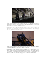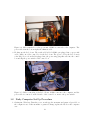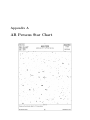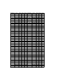
1
Periodicity of Variable Stars at the BYU-Idaho Livestock Center
Observatory
by
James Favaron
A senior thesis submitted to the faculty of
Brigham Young University - Idaho
in partial fulfillment of the requirements for the degree of
Bachelor of Science
Department of Physics
Brigham Young University - Idaho
April, 2015
BRIGHT YOUNG UNIVERSITY - IDAHO
DEPARTMENT APPROVAL
of a senior thesis submitted by
James Favaron
This thesis has been reviewed by the research committee, senior thesis coordinator, and
department chair and has been found to be satisfactory.
Date
Stephen McNeil, Advisor and Department Chair
Date
David Oliphant, Committee Member
Date
Brian Tonks, Committee Member
ABSTRACT
Periodicity of Variable Stars at the BYU-Idaho Livestock Center
Observatory
James Favaron
Department of Physics
Bachelor of Science
The BYU-Idaho Physics Department has a 250mm f/4 Maksutov Newtonian telescope for use at
the BYU-Idaho Livestock Center Observatory. In order for students to obtain images that can
be used for research, there are several setup procedures and techniques that need to be mastered.
These include procedures include the setup and dismantling of the telescope, as well as maintaining
the telescope and computers at the observatory. The techniques to be used involve learning how to
focus, track, take images, and calibrate images. The equipment available at the observatory allows
students to perform research on variable stars, which are stars that have brightness that changes
over time. This paper includes basic research completed on the topic of AR Perseus, which was
confirmed to be a variable star with a period of nearly 10.2 hours.
Acknowledgements
First and foremost I would like to thank my wonderful wife Elizabeth, for her constant motivation
behind every effort I expend toward our future, and for supporting me after countless late nights
at the observatory. Without her I don’t know where I would be able to find the desire to work as
hard as has been required the last couple years.
I would like to thank Dr. Stephen McNeil for providing guidance and information whenever
it was needed and for never giving up on me. Thank you for helping me to contribute to this
university in a lasting and meaningful way.
Without the help of Dr. Tom Davis, not only would the department not have access to such a
fantastic piece of equipment, but I would still be learning how to use it. Thank you for your selfless
devotion to the students of this department and for helping us to ever move closer to producing
significant scientific research.
Lastly, I would not have succeeded without the help of my colleagues. Matthew Brownell,
Forrest Hubert, and James McCulloch, without you I would be lost and frankly I would be miserable.
We all know how terrifying the goats at the Livestock Center are to listen to at 2:30 am during an
observation night, thank you for never making me go through that alone. You each contributed
enough to this project that you deserve as much credit as anyone for the current state of the
program.
Contents
1 Introduction and Background Information
1.1 Introduction . . . . . . . . . . . . . . . . . . . . . . . . . . . . . . . . . . . . . . . . .
1.2 Variable Stars and Their Importance . . . . . . . . . . . . . . . . . . . . . . . . . . .
1.3 Photometry History . . . . . . . . . . . . . . . . . . . . . . . . . . . . . . . . . . . .
1
1
1
2
2 CCD Technology and Previous Work
2.1 History of CCD Development . . . . . . . . . . . . . . . . . . . . . . . . . . . . . . .
2.2 Physical Principles Governing CCD Technology . . . . . . . . . . . . . . . . . . . . .
2.3 BYU-Idaho’s CCD Research Capabilities . . . . . . . . . . . . . . . . . . . . . . . . .
5
5
5
7
3 Telescope Preparation and Starry Night Operation
9
3.1 Daily Telescope Set-Up Procedure . . . . . . . . . . . . . . . . . . . . . . . . . . . . 9
3.2 Daily Computer Set-Up Procedure . . . . . . . . . . . . . . . . . . . . . . . . . . . . 12
3.3 Daily Closing Procedures . . . . . . . . . . . . . . . . . . . . . . . . . . . . . . . . . 17
4 Imaging Techniques
19
4.1 Focusing the CCD . . . . . . . . . . . . . . . . . . . . . . . . . . . . . . . . . . . . . 19
4.2 Setting up Tracking and Auto-Guiding . . . . . . . . . . . . . . . . . . . . . . . . . . 20
4.3 Image Calibration and Frame Captures . . . . . . . . . . . . . . . . . . . . . . . . . 20
5 Photometry
23
5.1 Setting-Up Storage Folders . . . . . . . . . . . . . . . . . . . . . . . . . . . . . . . . 23
5.2 Finding Objects in Starry Night, Syncing to Stars, and Taking Images . . . . . . . . 24
5.3 Performing Photometric Analysis . . . . . . . . . . . . . . . . . . . . . . . . . . . . . 26
6 Results, Program Direction, and
Future Projects
29
6.1 Results and Program Direction . . . . . . . . . . . . . . . . . . . . . . . . . . . . . . 29
6.2 Remote Access through LAN and
Additional Computers . . . . . . . . . . . . . . . . . . . . . . . . . . . . . . . . . . . 30
6.3 Internet Access, New Dome and Webcam Support . . . . . . . . . . . . . . . . . . . 30
A AR Perseus Star Chart
35
B Data
37
vii
C Information Cheat Sheet
41
List of Figures
2.1
The Anatomy of a Charged Coupled Device (CCD).
3.1
3.2
. . . . . . . . . . . . . . . . . . . .
CCD attached to Robofocus. . . . . . . . . . . . . . . . . . . . . . . . . . . . . . . .
Cables attached on the computers end. Note: It is important that COM1 be plugged
into the main spot on the motherboard, because that is the COM1 port that you
tell the program to use in order to mount the telescope. . . . . . . . . . . . . . . . .
3.3 Cables attached to the camera. From left to right the connections are: Unused,
Serial port for filter wheel, USB cable to computer, power cable. . . . . . . . . . . .
3.4 Cables attached to telescope mount. COM1 is connected to the computer. The
power cable is in the bottom right, the thinnest cable. . . . . . . . . . . . . . . . . .
3.5 Cables connecting to the Robo-Focus. COM2 connects to the computer, and the
power cable is connected on the left side of the control box, next to the power switch.
3.6 Syncing the computer time with the atomic clock. . . . . . . . . . . . . . . . . . . .
3.7 Opening the Observatory Controls . . . . . . . . . . . . . . . . . . . . . . . . . . . .
3.8 ASCOM Driver window with mount controls. . . . . . . . . . . . . . . . . . . . . . .
3.9 Camera Control window. . . . . . . . . . . . . . . . . . . . . . . . . . . . . . . . . . .
3.10 Connecting Starry Night to the telescope. . . . . . . . . . . . . . . . . . . . . . . . .
ix
6
10
11
11
12
12
13
14
15
16
17
x
Chapter 1
Introduction and Background
Information
1.1
Introduction
Astronomy has long been one of the most curiosity inspiring sciences for mankind to study
its place in the universe, as well as trying to learn more about our home on Earth by studying
stars and other planets. Because of the rapid rate at which technology has advanced in the recent
century, scientists have been able to develop devices and techniques to help us study the night sky
like never before. Charge-coupled devices (CCDs) are one of the newest tools that astronomers
have to help us in our quest for studying things like galaxies, nebulae, planets, and stars.
CCDs were not originally invented for astronomy or photography, but rather as a new method
of attempting to store data digitally for computer memory. It allowed for the use of a large value
of voltages to be used instead of only being able to use binary language. Later on it was seen that
CCDs had a fantastic ability to record images, and now they are used in the majority of studies
related to astronomy, as well as being used in most devices that can take images in normal daily
use.
In recent years, Brigham Young University-Idaho was able to acquire a 250mm MaksutovNewtonian telescope by way of donation from Dr. Thomas V. Davis. This telescope is meant
to facilitate and assist in research opportunities for students at the school to study the heavens
above in great detail. With this telescope, we have paired a SBIG ST-7 XME CCD camera that
contains two CCD chips in order to have one processing images while the other assists in helping the
telescope auto-track its target. These acquisitions have provided opportunities for many students to
participate in relevant research to the scientific community, and will provide even more opportunities
in the future.
1.2
Variable Stars and Their Importance
Variable stars are any stars that have a luminosity that changes over time. Typically their
luminosity follows a pattern of getting brighter and then dimmer and then repeating the cycle,
rather than just going from being dim to being brighter over the course of a long period of time.
When dealing with variable stars, the time it takes to go from its brightest luminosity to its dimmest
1
and then return to its brightest again is called a period. Periods of different types of variable stars
can range from just a few minutes to quite a few years, and everywhere in between.
There are many different types of variable stars, but in general they can be broken into six
general classifications[1] [2].
1. Rotating Variable Stars - RVS are stars that don’t actually change in brightness, but appear
to change in brightness from our point of view on Earth due to an irregularity in the shape
of the star, or the star might just be brighter on one side compared to the other.
2. Cataclysmic Variable Stars - CVS’s brightness change due to thermonuclear processes happening within the star. These were originally referred to as novae, which means ‘new’ in
Latin, due to having a sudden burst of energy that made a star visible in the sky that was
normally not able to be seen by the naked eye.
3. Eclipsing Binary Stars - EBS are systems of at least two stars that orbit in such a way that
they periodically eclipse in the field of view from Earth. This causes the overall apparent
magnitude of the system to change with respect to the observer.
4. Eruptive Variable Stars - EVS show differences in brightness due to material being lost from
the star in the form of stellar flares. They can also happen when accretion takes place and
material is added to the star.
5. Pulsating Variable Stars - PVS swell and shrink which affect its luminosity. These pulsations are broken into two categories which are radial, where the entire star is expanding or
contracting, and non-radial, where only a portion of the star expands while another part
contracts.
6. Optically Variable X-Ray Sources - These are stellar objects that produce X-rays that can be
monitored in order to gather information about them, but they require specialized equipment
that we do not have access to at BYU-Idaho.
AR Perseus is the star that was studied for the duration of this research. It is a more specific
type of pulsating variable star (PVS) called an RR Lyrae star, and even more specifically is part of
a class known as Cepheid Variable Stars. Cepheid Variable stars are special because they can be
referred to as ”standard candles” and given information gained from studying them, it is possible
to know how far away they are from Earth. This star is located in the constellation Perseus and
has a period of roughly 10.2 hours.
1.3
Photometry History
In astronomy and astrophysics, photometry is the process of measuring the amount of light
coming from stars in the night sky in order to calculate their brightness. By utilizing photometry,
astronomers are able to find information regarding brightness and magnitudes of stars, as well
as the distance to the stars and other objects nearby. By using specific filters and devices, you
can also gather information regarding a star’s composition and temperature, which can help to
categorize them and find what stage of their life they are in. Many different research endeavors
2
utilize photometry including, but not limited to, studying variable stars, supernovae, active galactic
nuclei (AGN) and searching for planets outside of our solar system.
A unique tool that has allowed us to develop photometric capabilities for research is the chargedcoupled device (CCD). The specific CCD has been used by several other students in the past in
order to take astrophotography images and perform photometry as well. It has two CCD chipsets
built into one camera that allows data to be taken by one chip, and tracking information to be
gathered by the other chip in order to accommodate following the star through the night sky for
long exposure times.
Being able to perform photometry with the help of a CCD allows us to see exactly how much the
brightness of a star changes over time. Because of this, we are able to compare other information
to the average brightness of the star to find out how far away it is, along with other objects that
are in its vicinity. By utilizing this process, mankind has been able to better find its place among
the stars and how we relate to our cosmic neighbors.
3
4
Chapter 2
CCD Technology and Previous Work
2.1
History of CCD Development
CCDs are what allow the work at the observatory to be achieved and it is imperative to understand
how they work and why this impacts future research possibilities. The CCD was invented 1969 at
AT&T Bell Labs by Willard Boyle and George E. Smith. They came up with the idea for the device
while they were working on semiconductor bubble memory. Originally when they came up with
the design they coined their new invention ”Charge Bubble Devices”. The original idea behind the
design was to transfer charge from the surface of a semiconductor to a storage capacitor. There
was also a device being developed at Philips Research Labs during the late 1960’s as well called
the bucket-brigade device, or BBD, that was trying to accomplish a similar goal.
The first paper outlining the Charge Bubble Device listed many possible uses which included
being used as computer memory, a delay line for electric circuits, and lastly as an imaging device.
The first working CCD was a simple 8-bit shift register. A shift register is an array of flip flops in
a digital circuit that all share the same clock. These flip flops are connected in a way that sending
data into one shifts the data over throughout all of them. This enables the shift of a bit array that
is stored inside it by one position. This device was designed to be used as memory for computers,
similar to what we use random access memory (RAM) for today.
Development began to increase rapidly with many companies attempting to get involved in
the CCD market. By 1971, Bell researchers had been able to capture images with simple linear
devices. Several other companies including Sony, Kodak, RCA, Fairchild Semiconductor, and
Texas Instruments quickly jumped on board and began development programs related to CCDs.
An electrical engineer at Kodak named Steven Sasson was the first to invent a digital camera using
a Fairchild 100 x 100 array CCD in 1975. In 2009, Boyle and Smith were awarded the Nobel
Prize for Physics for invention of the CCD concept, and over the past decade they have received
numerous other awards for the work they have pioneered.
2.2
Physical Principles Governing CCD Technology
CCDs consist of arrays of photodiodes. These are what help the chip to convert photons (light)
into an electric charge. When light comes in and hits a photodiode, there are electrons that become
excited out of the valence shell of the silicon that contains the diodes. There is a depleted layer of
5
Figure 2.1: The Anatomy of a Charged Coupled Device (CCD).
silicon that then captures this free electron. When doing work in astronomical observations, such
as photography or photometry, the CCD is exposed to light for a specific amount of time that we
call the exposure time. During this exposure there are many photons that enter in and strike the
CCD. Over time, more photons excite electrons along the silicon lattice, which makes more and
more electrons become stored in the different individual potential wells. Once the exposure time is
completed, the CCD then moves the charge through its gates and the computer is able to record
an Analog Digital Unit (ADU) which can then be used on the computer as data.
An important step in helping us determine the uncertainty and precision involved with a specific
CCD’s measurements is determining the value of the chip’s Gain. Gain is defined as a ratio of the
amount of electrons in a full well to the maximum ADU value possible. Specifically with the CCD
at the BYU-I observatory there is a maximum ADU value of 65,535 per pixel. The maximum
number of electrons in any one single pixel is 90,000.
Gain =
ElectronsinaF ullW ell
M aximumADU V alue
=
90,000
65,535
= 1.37
This shows that for every 1.37 electrons captured by an individual pixel in the CCD, the ADU
value the computer reads increases by 1. The closer of a one-to-one correspondence, the more
accurate the readings of the CCD will be. Computers that are connected to the CCD with imaging
software are able to read these ADU values and produce an image. These images can be so accurate
that the software can tell on its own where a star begins and ends, due to the sharp drop off in
ADU from one pixel to another. Being able to read the ADU values also helps the software do
image recognition while finding objects in star fields automatically by comparing the ADU values
in each image taken. This will be touched on more in Chapter 4 when dealing with methods of
performing photometric analysis.
6
2.3
BYU-Idaho’s CCD Research Capabilities
Because BYU-Idaho has a good quality CCD paired up with our telescope, there are several
options available for students to research. There are several celestial objects visible from Rexburg’s
night sky that could be photographed using astrophotography and these images could be print
worthy for using in the department as well as submitting to journals or even possibly the astronomy
picture of the day (APOD) through NASA. There is also the opportunity present to improve upon
the photometric processes that have already been established, as well as diving into the data
reduction and analysis side of photometry. Photometry will be discussed in detail later in this
paper, but a particular topic of study that has not been touched on yet by students is that of doing
astronomical spectroscopy.
Astronomical spectroscopy is the use of spectroscopy to measure the spectrum of electromagnetic
radiation with celestial objects. This radiation comes in the form of visible and non-visible light
and can be used to collect a host of information about objects that help us to learn more about
their behavior and composition. Some of the properties that can be studied include chemical
composition, temperature, density, mass, distance from Earth and relative objects, luminosity, and
relative motion.
The Physics department has also procured a new set of filters to place on the camera for the
telescope. In order to perform broad band filter and narrow band filter imaging, these will need to
be installed and the computer will need to know which is which. One of these filters is a hydrogen
filter, which will help students be able to determine the amount of hydrogen content in a star and
determine how far along it is in its lifecycle. There will also need to be significantly more work done
with the auto-guiding CCD in order to get the best form of tracking that the telescope’s mount is
capable of, and doing this will enable longer exposures for more detailed measurements. There are
currently a few different things holding the program back from being able to perform spectroscopic
observations, but none are too far out of reach.
7
8
Chapter 3
Telescope Preparation and Starry
Night Operation
This section will encompass what goes into setting up and shutting down the telescope on a daily
basis, as well as things that need to be addressed for maintenance over a period of time. Some of the
steps within this documentation may or may not need to be performed due to the consistency of the
telescope usage and whether or not certain events transpire (such as someone tripping and knocking
the telescope out of sync). Anywhere that there is a conditional instruction, it will be noted as
such, but the default should be to perform each task every night of attending the observatory unless
otherwise noted[3].
3.1
Daily Telescope Set-Up Procedure
1. Removing the tarp from the dome: The telescope resides in a dome that is behind the main
building, and this dome will have a tarp on it that is attached to the dome by bungee cords.
Remove these and bring the tarp inside the building and lay it on the table with the bungee
cords.
2. Opening the dome: The desk that the computer resides on has only one drawer, and inside
this drawer is a key attached to a purple lanyard. This is the key used to unlock the door on
the dome. After opening the door you will see two knobs on the inside of the wall above the
door. These are the mechanisms that keep the dome closed, unscrew them and put them on
the desk. Once the door is unlocked, place the key back in the desk.
3. Removing tarps from the telescope: Once inside the dome, remove the two covers from the
telescope. There is one that is on the telescope itself that is a tarp, and one that is on the
counterweight that is more of a canvas material.
4. Attaching the camera: This step will only need to be done at the beginning of a viewing
season, as it is permissible to leave the camera attached when leaving for the night, but
should not be left on during long periods of inactivity at the observatory. When attaching
the camera, insert it into the Robo-Focus and align it to where the rails are parallel with the
9
telescope. Secure it in place by using the screw (located on the right in the photo) until it
sits snug. Pull up on the rails slightly to ensure that the camera won’t move.
Figure 3.1: CCD attached to Robofocus.
5. Hooking up the cables to the computer: There is a tube of cables that run from the computer
to the telescope. The end of these cords never need to be unplugged from the computer, and
they are labeled (see Figure 3). The other ends need to be run to the dome and contains
three plugs.
10
Figure 3.2: Cables attached on the computers end. Note: It is important that COM1 be
plugged into the main spot on the motherboard, because that is the COM1 port that you tell
the program to use in order to mount the telescope.
6. Hooking up the camera: Take the USB Cable and plug it into the camera (see Figure 4).
There is a power cord from the power strip inside the dome that runs to the camera, plug
that in as well and the camera is hooked up.
Figure 3.3: Cables attached to the camera. From left to right the connections are: Unused,
Serial port for filter wheel, USB cable to computer, power cable.
7. Hooking up the mount: The serial cable labeled COM1 needs to be plugged into the top of
the two serial ports on the mount. This establishes its connection to the computer. There is
a power supply on the ground in the dome that is connected to the power strip on one end
and to the mount on the other end, this cable is ok to be left plugged in indefinitely.
11
Figure 3.4: Cables attached to telescope mount. COM1 is connected to the computer. The
power cable is in the bottom right, the thinnest cable.
8. Hooking up the Robofocus: The serial cable labeled COM2 gets plugged into a grey serial
cable coming out of the control box for the Robofocus. The power cord for the Robofocus is
a 12v DC power cord and is left plugged into the power strip, plug this cable into the control
box and flip the power switch on the control box.
Figure 3.5: Cables connecting to the Robo-Focus. COM2 connects to the computer, and the
power cable is connected on the left side of the control box, next to the power switch.
3.2
Daily Computer Set-Up Procedure
1. Getting into Windows: Turn the power on and type the username and password provided on
the computer’s case. If the username or password change, update the labels on the computer
case.
12
2. Sync the Clock: Open up an internet browser and navigate to
http://www.time.gov, and select Mountain Time 12-hr. Click on the clock in the bottom
right corner of the screen to open up the Windows clock and Calendar. Click ”Change date
and time settings...” Click on ”Change date and time...” Set the computer’s clock to be in
sync with the atomic clock then exit the windows for changing the time, as well as the internet
browser.
Figure 3.6: Syncing the computer time with the atomic clock.
3. Open necessary programs: There are shortcuts to MaxIm DL 5 and Starry Night Pro Plus 6
in the center of the desktop. Start by double clicking MaxIm DL 5.
4. Open Observatory Control: Click the ”Toggle Observatory Control” button to bring up the
Observatory Control window as shown.
13
Figure 3.7: Opening the Observatory Controls
5. Connect the telescope: In the telescope area, click the ”Connect” button, (Note: If the words
”No Device Selected” appear in the window, click the little black arrow and choose the mount,
then click ok, then connect the telescope.) and a window will appear that asks you to confirm
the ”unpark position”. Click ok.
6. Open the Ascom window: Once you have connected the telescope, a new icon will appear
in the bottom right corner of your screen that looks like two little blue circles. Click this
and it will bring up the ASCOM Driver window. Click Expand at the top of the window so
you can have access to all of the information. If the window is ever closed, bring it back by
clicking the button in that tray. This window should be kept open at all times when using
the telescope, as it has an emergency stop button located in the lower left corner that allows
the telescope to be stopped immediately in the event that any cables get tangled.
14
Figure 3.8: ASCOM Driver window with mount controls.
7. Connecting the camera: Click the Camera Control icon and it will open this window. It
should say ”SBIG Universal” under Setup Camera and under Setup Filter. If it does not,
then click the Setup Camera button and choose SBIG Universal under ”Camera Model”, and
ST-7 under ”Connect to”. The following three options should have the following settings:
Swap Chips - ”No”, Guide Chip - ”Internal”, Ext. Trigger - ”Off”. Open the ”Options” for
Camera 1, and make sure there is a check mark next to ”Auto-dark” Subframe Extraction.
Click ok. Then click ”Connect” in the top right corner of the window, and then click ”On”
under coolers. Click on the ”Expose” tab at the top of the Camera Control window.
15
Figure 3.9: Camera Control window.
8. Connecting to Starry Night: Minimize MaxIm DL and double click on Starry Night Pro Plus
6. Starry Night asks to be updated whenever it is opened, if there is internet access to the
computer, then update it, otherwise it does not need to be done. This doesn’t update the
program itself, just the database of where things will be at any given time in the sky, so it
knows where the desired objects. Once Starry Night has loaded, click the ”Telescope” tab on
the far left side of the window. It will bring out a menu, click ”Connect” under the Setup
submenu, at which point the current Right Ascension, Declination, Altitude, and Azimuth
numbers will appear in the Status submenu[4].
16
Figure 3.10: Connecting Starry Night to the telescope.
The telescope and camera are now connected exactly how they should be. From this point
images can be taken and the telescope can be moved using both Starry Night and MaxIm DL
5.
3.3
Daily Closing Procedures
When closing up for the night, it is very important follow this order to keep everything in working
order.
1. Park the telescope by clicking the “Park” button in the ASCOM Driver window. Click “K”
in the prompt that appears.
2. Disconnect the telescope in Starry night by clicking the ”Disconnect” button under the Setup
submenu in the Telescope tab.
3. Close Starry Night by clicking the ‘X’ in the top right corner of the window. When it asks
to save changes, click “Don’t Save.”
4. In MaxIm DL 5, open the Camera Control window, and click the Setup tab. Click the ‘Warm
Up’ button on the right side of the window, this slowly warms the CCDs temperature up.
The cooler power will slowly drop in percentage and in the summer, the sensor temperature
17
should slowly rise in the summer, and in the winter it might drop a little bit due to ambient
temperature. Click Disconnect in the top right corner of the window, and close the Camera
Control window.
5. In MaxIm DL 5, open the Observatory Control Window, go to the Setup tab, click ”Disconnect” under the Telescope area. This will close the ASCOM Driver window as well.
6. Close MaxIm DL 5 by clicking the ’X’ in the top right corner of the window.
7. Shut down the computer.
8. Turn off the Power Switch on the power supply for the Mount, turn off the Power Switch on
the control box for the Robo-Focus.
9. Unplug the power strip from the extension cord, and coil the extension cord up. Place the
cord for the power strip into the dome, and the extension cord back into the observatory.
10. Unplug the USB cord from the camera, the COM1 serial cable from the mount, and the
COM2 serial cable from the Robo-focus. Take the tubing of cable and coil it back up, place
it next to the desk inside the observatory.
11. Replace the tarp and canvas cover to the telescope and counterweight respectively.
12. Close the lid to the dome, put the knobs back in to hold it in place, lock the door.
13. Replace the tarp on top of the dome and secure it with bungee cords. Lock up the observatory
when leaving.
18
Chapter 4
Imaging Techniques
4.1
Focusing the CCD
In order to take quality pictures, whether for simple astrophotography or research, the camera
must be focused. This section will discuss focusing by both manually turning the focusing knobs,
and manually adjusting them with the Robo-focus control box. The Robo-focus does have the
capability to be an automatic focuser on the computer, but currently cannot be used due to only
having one working serial port on the computer. Once this issue is resolved, students can review
the user’s manual from the Robo-focus and connect it through MaxIm DL 5.
This will be done once the telescope has been pointed at the desired object. It is good practice
to find objects in the sky to become familiar with, and then use those same objects on a nightly
basis. The experience from seeing the same object multiple times will help expedite the focusing
process due to knowing what the final focused image should look like.
1. Begin by using Starry Night to point the telescope to the desired object.
2. Open the Camera Control window in MaxIm DL 5, click the Expose tab, and set the picture
to a 1 to 5 second exposure. The exposure time will depend on the brightness of the object.
If there is noticeable tearing of the image, it is because the exposure time was set too long.
3. Set binning to 1x1.
4. Make sure the camera is set for continuous shots.
5. Set the delay to 4 or 5 seconds, possibly more if it is hard to keep up with the continuous
images.
6. Click start and watch the images come through.
7. There is a graph in the bottom left corner that shows how sharp the images are. The focus
will need to be adjusted until the peak in that image is as sharp as possible. If the the
adjustments take the camera beyond the focusing point, the peak will start getting more
broad, and that shows that it is it time to start turning the knob the previous direction.
8.
• If the Robo-focus is not being used, used the knobs on the telescope. The two large
black knobs are rough focusing knobs while the gold knob is a fine focuser.
19
• If the Robo-focus is being used, use the control box to move it in and out of focus with
the two red buttons.
9. Once the image is focused to the best it can be, turn off the continuous shot and prepare to
take images.
4.2
Setting up Tracking and Auto-Guiding
There are several different options to track the sky with the ASCOM driver for a GTOCP3 mount.
The buttons are located in the bottom left corner of the driver window, and from left to right they
are as follows:
1. Stop - Stops all movement of the mount, and should be used if any cords are going to become
tangled or the telescope is going to hit something. Never hesitate to hit to stop button.
2. Sidereal Tracking - Sidereal motion is the movement of the stars that makes them appear to
to rise and set, which is caused by the rotation of the earth. This option moves the telescope
exactly opposite of what the sidereal motion is, in an attempt to keep fixated on one location.
The mount moves at a rate of 15.0 arcseconds per sidereal second.
3. Lunar Tracking - The Lunar tracking rate is an average lunar rate in right ascension only.
More precise lunar tracking including declination movement can be accomplished with the
custom rates described below. The mount moves at a rate of 14.685 arcseconds per second.
4. Solar Tracking - The solar tracking is similar to the Lunar tracking, but moves at a rate of
15.0 arcseconds per second.
5. Custom Tracking - In the custom tracking options the rate is set by the user in a value of
seconds per sidereal second in the right ascension and arcseconds per second in the declination.. This allows the following of objects like comets that do not have as much of a regular
path in the sky as other celestial objects.
Outside of the ASCOM driver, MaxIm DL will allow the use of the secondary CCD chip in the
camera to be used for Auto-Guiding. This is useful for long exposure times, because it takes the
same portion of the sky that is being imaged, and watches it for differences. Once a star moves and
creates a difference in the image, it moves the mount to counteract the small difference and keeps
the camera focused on the same portion of the sky. This is the most accurate option for tracking,
but has not been fully utilized in MaxIm DL yet, due to time constraints and the weather. Using
the manual for MaxIm DL and exploring the options in the Camera Control window, one could
figure this out very quickly and use it to produce fantastic images and research data.
4.3
Image Calibration and Frame Captures
There are many different types of errors that can be induced into images from sources other than
focusing and tracking. For the most part, the errors are encountered due to extra electrons being
introduced to the CCD from various sources. It is impossible to distinguish between these additional
20
electrons, and the photoelectrons coming from the star, so image calibration helps to reduce the
amount of errors that are induced into the images. There are three specific types of calibration
images that will be discussed here: bias images, dark frames, and flat fields[5].
A bias frame is one that is taken with essentially zero exposure time, to where the shutter never
even opens to take the image. The resulting image is one that shows the inherent noise levels that
are associated with the CCD itself and is further transferred into each image that is taken by the
CCD. The best practice for making a good bias frame, is to take 20 or more of them and average
them together.
A dark frame is also taken with the shutter being closed, but for the duration of time matching
that of the duration of time for the images that are intended to be taken. If taking 90 second
exposure images is the current goal, then your dark frames will also be 90 second exposures. These
measure the amount of thermal noise, or dark current, found on the CCD chip during exposure
time. This helps show pixels that are ”hot” on the CCD, that read higher than average pixels. If
the feature is not being used to take automatic dark frames, take 20 or more of them and average
them together.
A flat-field image corrects variations between the thousands of pixels on the CCD. Flat-fields
are taken by opening the shutter and taking an image of a uniform field. This can be done just
after sunset or just before sunrise, when there is no sun or stars in the sky, and the sky is a
uniformly light-blue color. Flat-fields can also be used by holding a grey or white shirt in front
of the telescope, as long as it’s uniform. Fortunately, at the observatory there is a flat-field panel
that is essentially a giant white panel to be place in front of the telescope so that flat-fields can be
taken any time[6]. For flat-fields, take 10 or more and average them together.
Once the calibration images have all been taken, it’s time to set calibration to actually correct
our images. Normally it would be necessary to take dark frames into consideration while doing this,
but MaxIm DL 5 has an option to take dark frames each time it takes images and automatically
correct them on the spot. To finish the calibration, bias frames and flat-fields remain.
1. After opening MaxIm DL 5, open all of the images that need to be corrected.
2. Click the Process menu at the top of the screen, then click Set Calibration...
3. In the middle of the window, click clear all groups to start fresh.
4. Under the Source folder section, click the yellow folder icon and browse to the folder where
the bias frames and flat-fields are stored. Select the folder and click ok.
5. Click the Auto-Generate (Clear Old) button.
6. Click Ok in the top right corner.
7. Now click the Process menu, and click Calibrate all.
8. All images that were open in MaxIm DL at this time are now calibrated.
21
22
Chapter 5
Photometry
5.1
Setting-Up Storage Folders
When working at the observatory, a lot of detail will be involved in storing and maintaining data.
An incredible amount of data can be produced in a very short amount of time, leaving the task of
keeping it all organized to seem quite daunting. Using the methods described here, data can be
secure and organized for many people that desire to use the observatory simultaneously[7].
1. Under the documents folder of the observatory computer, there will be a folder labeled ”Observatory Data”.
2. Each student should have a folder that is named based on the year they create it , and their
last name. For Example ’2015 Smith’
3. Inside that folder will exist a separate folder for each night of data that is taken. If data was
taken by Smith on the 25th, 26th, and 27th of April, there would be three folders each named
’04-25-15’, ’04-26-15”, ’04-27-15’ respectively.
4. Inside each daily folder, there should be a folder for ’Calibration Images’ where all bias frames,
flat-fields, and (optionally) dark frames should be placed.
5. There should also be an ’Images’ folder, where all actual photos taken will be saved.
6. Any other data such as star charts, Word/Excel documents, viewing plans, etc, can be saved
in the main folder for that date.
Backing up information is extremely important not just because it’s desirable to not lose all
the work that’s been done, but also due to the fact that the weather dictates when work can be
done at the observatory. It is not always possible to just repeat the work that’s already been done,
simply because the weather might not allow it for a considerable window of time, and when it does
allow it again, the object that was observed may no longer be available for some time. There have
already been instances of possible data loss at the observatory and because of this there are extra
avenues of backup being investigated. For now, utilize the external hard drive that is attached to
the computer, as well as the USB flash drives that are located in the desk, in order to back up data
each night.
23
5.2
Finding Objects in Starry Night, Syncing to Stars, and Taking
Images
Starry Night Pro 6 is planetarium software that allows the viewing of objects in the sky. It also
doubles as a powerful tool when hooked up to a telescope, as it can direct the telescope to the
objects being investigated automatically. In order for this to work properly, it must be synced up
with objects in the sky so that it’s aware of where things are in relation to each other. MaxIm
Dl also has this capability, but the built in software leaves much to be desired in terms of visuals,
which is why Starry Night is utilized instead.
To use the search function and slew to objects in Starry night[8]:
1. Open Starry Night.
2. Click the find tab
3. Either find an object on the preset list and double click it, or type an object into the search
bar and hit enter.
4. Right click the object you want to see, find ’Slew to (object name)’ in the list, and click. The
telescope will now move to the object.
5. While it’s slewing, make sure to watch the cables that are attached, as this is the most likely
time that there will be a cable issue. Be prepared to have someone hit STOP on the ASCOM
driver at all times, or hold the mount controller and be prepared to press stop.
6. After slewing, take an image in MaxIm DL. If the object is on the screen, right click in the
center of it, and click ’Slew here’. It may take 2-3 times of doing this on the same object
to get it centered in the middle of the screen. Once it is centered, it is time to sync to the
object.
If it has been a long time since the last time the telescope was used, or the telescope has been
severely bumped, it may not find the object it was searching for. In this case, it will be necessary
to use the hand controls for the mount and find the desired object manually. Once multiple objects
are found and synced with, the telescope will be able to follow steps 1 through 5 again. These next
steps will be performed after finding a desired object in the sky and confirming that it is in fact
the object you want to sync to. Be sure it is the correct object, or it will profit nothing to sync to
it.
• To sync to a star in Starry Night, right click the star, click ’Sync to (star name)’.
• To sync to a star in Maxim DL - Open observatory control, go to the Zoom tab, find the star,
right click it and click ’Sync to (star name)’.
In order to have accurate syncing, it is important to sync to at least 3 stars, and to make them
be a significant distance across the sky from each other. Once both programs have been synced to
3-4 objects, Starry Night should be able to locate any desired object and put it within the viewing
angle of the camera.
24
After syncing to stars and being able to find the desired objects, taking images is now possible.
There are two different ways to take images, either taking a single images at a time, or programming
MaxIm DL to take the multiple photos in an order that will eventually take all the necessary images,
and place them in a specific folder together.
To take a basic single image:
1. Open Camera Control.
2. Click Expose tab.
3. Set Exposure Preset to Find Star.
4. Set X binning and Y binning both to 1.
5. Click the ’Single’ button on the right side of the window.
6. Click the options arrow, under calibration, make sure the Auto Dark option is selected.
7. Set the desired exposure time at the top of the window.
8. Click start to begin taking an image.
Upon doing this, the camera will take two images, of the same length of exposure. One will be
a dark frame that will be automatically subtracted and the other will be the desired image.
Most of the time it will be extremely tedious to take a single image at a time given the several
images are necessary at the same time. Here are the steps to program MaxIm DL to take multiple
images and automatically save them for you.
1. Open the Camera Control window.
2. Go to the Expose tab.
3. Click the autosave button.
4. Under the Autosave Filename in the top left corner, choose the formatting for the file names
of the images.
5. Under Delay first, type the amount of seconds of a delay between clicking Start and the first
image being taken.
6. Under Delay between, type the amount of seconds between each image, to the start of the
next dark frame.
7. Under Slot one, select the type of image, bias, flat, or light. Select the filter to be used,
and the suffix on the file names of that type. For example, if the image names are to be
saved as pictures and there will be red filter, blue filter, and green filter images taken, it can
automatically save them all as picturesR, picturesB, and picturesG respectively.
8. Set the length of exposure for each image, and set the binning to 1. Under repeat, select the
amount of images of that type to be taken.
25
9. In the top left corner, under Estimated Duration, the total time for the program to finish will
be calculated.
10. Click Apply in the top right corner, then click OK.
11. Back in the Camera Control window, click on the Autosave button, and specify the folder for
the images to be saved to.
12. Click start and it will now finish in the Estimated Duration time, saving all of the images to
the folder that was specified.
While performing photometry, the programming method is the most useful method for taking
images. Some stars need to be observed for 4-5 hours before being able to see any difference in their
brightness, so setting up a 30 second exposure every minute and a half or so, for 5 hours straight,
is a great way to let it automatically take the data all by itself. During this time is when the screen
simply needs to be monitored to make sure the images are not becoming off centered, and other
tasks such as homework or observatory maintenance can be done. Once all the images are finished
being taken, the next step is analyzing them to verify the magnitude and variability of the desired
star.
5.3
Performing Photometric Analysis
Once all of the images have been taken and calibrated, it is now time to do some photometric
analysis. MaxIm DL makes this process very simple, but requires some information from the star
field.
There will need to be a star in the images that has a constant magnitude, and this is called the
Reference Star. The program will look at this star as something to be considered constant, and
can then tell the variability of the Object Star (the one being studied) based upon that and the
ADU values for each image. It will also need another constant star somewhere in the field called a
Check Star. The check star primarily exists to make sure that the Reference Star isn’t actually a
variable star itself. In practice the Reference Star should have a lower magnitude than the Check
Star.
1. Open MaxIm DL 5, and open all of the images to be analyzed.
2. Go to the Analyze Menu at the top of the screen, and click Photometry, this will bring up a
Photometry window and an Information window.
3. In the Photometry window there is a list of all the images that are open. If any of them
need to be removed from the set (maybe a satellite flew across the sky during the image
being taken so there is a streak of white across the image) simply scroll through and find that
image, click it, and click Exclude.
4. In the Photometry window, click the drop down arrow underneath ’Mouse click tags as:’ and
select New Object. Place the cursor over the correct star and click the mouse. This will
now find that same star in every open image. It might take just a moment depending on the
number of photos. The aperture may need to be re-sized to fit the size of the star. To do
26
this right click on the screen near the star after the star has been tagged as Object 1, and a
menu will appear that has options for Set Aperture Radius, Set Gap Width, and set Annulus
Thickness. When setting the aperature radius, try not to make it so small that it excludes
any part of the star, and leave a little bit of black around the edge of the star.
5. Next set the Reference star. Go to the Photometry window, click the drop down arrow
underneath ’Mouse click tags as:’ and select New Reference Star. Select the reference star
and then input the magnitude of the reference star in the spot labeled ’Ref Mag’.
6. Proceed to set the Check star the same way as the Reference star, except this time it does
not require putting in the star’s magnitude.
7. At this time it is a good idea to scroll through all of the open images and make sure that
every one has been appropriately labeled with your Object, Reference, and Check Stars. This
should only take a moment, even with several hundred images.
8. Click View Plot, and the data will appear. At this point there will be three plot lines, and
at least one will be constant at the magnitude of the Reference star. The Check star might
be varying slightly, but more than likely it was a very faint star to begin with and things
like atmospheric conditions made it slightly different from image to image. The variable star
itself should appear to be varying in brightness over time.
9. Click Save and navigate to the folder that it needs to be saved in.
10. Close out of MaxIm DL and navigate to the folder the file was saved to. Double click it and
it will automatically open into Excel. Now there is data created for the variable star from
the images, to be presented in whatever manner is necessary.
27
28
Chapter 6
Results, Program Direction, and
Future Projects
6.1
Results and Program Direction
In the end, it was confirmed that AR Perseus is in fact a variable star, with a maximum magnitude
of 10.70 and minimum magnitude of 9.91. This agrees with the values given by the AAVSO for AR
Perseus. The resulting period was on the order of 10.2 hours, which was the period given by the
AAVSO.
The purpose of the work that has been done at the observatory for the last two years had two
directions in mind. Not only was there a goal determining the variability of a specific star, which
was accomplished, but to set up and lay a foundation for a program in which future students would
be able to push beyond the current issues that have prohibited the growth of a telescopic research
program at BYU-Idaho. Those barriers were
• An inconsistent level of work and visitation to the observatory.
• Only one student at a time, who was soon to graduate, being involved at the observatory and
taking their knowledge and experience with them.
• Not having an effective way to communicate information through student generations other
than through the most current senior thesis.
• The burden of one faculty member having many students working underneath them makes it
different for one faculty member to handle the amount of students interested in participating.
Every program and policy that has been implemented in the Telescopic Research Program has
attempted to over come one or more of these challenges, in an attempt to set up a program that
will flourish year after year and provide a place that many students at once can collaborate and
explore the heavens in an attempt to find both spiritual and secular truth. In order to assist in this
goal, the program now has access to an iLearn page that so far contains three separate sections of
information for students in the program.
• There is a resources section that contains information regarding how to navigate the page,
and what steps to take to prepare oneself to do research at the observatory. This section also
29
provides helpful links that students will need information from, as well as contact information
of individuals that are friends and colleagues of the program.
• There is a discussion board where students can discuss what times they want to meet at the
observatory, what changes they have made to equipment or programs, or share insights and
answer questions from the readings.
• There is a section devoted to posting reading materials that have been acquired from previous
students, or from free versions of books written by professors at other universities. These are
the resources Brother McNeil would normally have students read in print, but there was only
one copy of them and a large number of students joined the program this semester. This
makes it more manageable for Brother McNeil to tend to the needs of multiple students
trying to do work at once.
As students continue to use this page and work to increase the amount of content on it, it will
prove to expedite the process of catching students up to the most current work being done, so they
can focus more time on expanding the work rather than catching up.
6.2
Remote Access through LAN and
Additional Computers
During the Winter months in Rexburg, from around November until April, the observatory gets
shut down due to the temperature outside. The computer sits next to a set of double doors that
need to be open for cables to run outside into the dome. The only physical reason the temperature
makes a significant different is due to the comfort level of whoever is using the telescope, not
because it prevents the telescope from operation.
Because the observatory is not in operation for such a large portion of the year, there are many
things that have not had the chance to be observed by the BYU-Idaho Physics department. In an
attempt to remedy this issue, I have set up a LAN (local area network) out at the observatory that
has no outside internet access, but allows computers to connect locally through the network. Using
this new capability, the option is now available to use a remote access client built in to Windows
to use the telescope and take images from inside of the building in the warmth.
Another benefit to this remote access and being inside, is that it allows the user to monitor
the images being taken while working on other things. This means students monitoring a variable
star for 3-4 hours during a night can sit inside the building with books and homework and keep
continuing to work on coursework, therefore lowering the burden that student research puts onto
their school schedule. In order to better facilitate the learning experience of future students, the
program has acquired two new computers to put at the facility for the use of allowing students to
remotely access the telescope with one computer, and use the other for doing homework assignments
and projects for coursework.
6.3
Internet Access, New Dome and Webcam Support
In the previous section it was discussed how remote access over a LAN provided benefits to the
research program. In the Summer of 2015, there are plans to extend BYU-Idaho’s network to the
30
observatory, and thereby giving internet access to the observatory in the process. Once there is
internet access, an overwhelmingly numerous amount of new opportunities will become present.
Given access to the internet, the same process of remoting into the telescope over a LAN couple
be replicated to remote into the telescope from anywhere in the world, including from mobile
devices. This more than likely will be used for being able to remote into the telescope computer
to do data analysis while being at home or school, but this also leads to opportunities to perhaps
do collaborative research with other universities or allowing mutual use of equipment over the
internet. These options are not even in the planning phases yet, but they are options in the future
nonetheless.
In order to really be able to do any kind of remote access from outside of the observatory, a
minimum of two things need to take place. Number one is that the department needs a new dome
that can be controlled by the computer. MaxIm DL has the capability to utilize dome control,
but the current dome is a basic, none electric dome. If the school is to purchase a new dome, it
has been proposed to purchase a clam-shell type dome that opens from the center, instead of one
of the the hemisphere overlapping into the other side like the current dome. The current model
removes the possibility of ever observing the sky directly above the telescope, and makes it difficult
to find objects to track that will never go immediately through the top. The next thing that
would be necessary is a high definition webcam that would be mounted on the side of the building
or the dome, in order to view the cable situation from afar. The goal with this is to be able to
monitor whether or not any cables have a potential to become entangled or have too much tension.
This would be necessary since the option of physically walking outside and checking would not be
possible while remoting in.
31
32
Bibliography
[1] John R Percy. Understanding variable stars. Cambridge University Press, 2007.
[2] Barbara Ryden and Bradley M Peterson. Foundations of astrophysics. Addison-Wesley, 2010.
[3] Dr. Thomas V. Davis. Painting with Star Light kernel description, 2014.
//tvdavisastropics.com/.
URL http:
[4] Diffraction Limited. Introduction to MaxIm DL kernel description, 2008.
[5] Steve B Howell. Handbook of CCD astronomy, volume 5. Cambridge University Press, 2006.
[6] Starizona. Calibration Images kernel description, 2000.
[7] John Blackwell. Photometry Time Series kernel description, 2011. URL https://www.youtube.
com/watch?v=wCM7835SnwU.
[8] Imaginova. Starry Night Pro Plus User’s Guide kernel description, 2005. URL http://www.
starrynight.com/download/product_manuals/Pro_Plus_5_manual.pdf.
33
34
35
Appendix A
AR Perseus Star Chart
36
Appendix B
Data
Here are the plots created by both MaxIm DL and by Excel for the data gathered on AR Perseus.
The MaxIm DL plot only shows one night, because it has a difficult time eliminating the gap in
between observing nights and the data points become scaled enough that nothing can be gained
from looking at the graph.
The second plot is made from three separate nights of observing, where the second two nights
happened to be during the same portion of the star’s period as the latter half of the first night of
viewing, and this is what causes the overall shape of the graph repeating to drop down from the
peak.
The following two pages contain the data points gathered from observing AR Perseus. The
datapoint column is simply the chronological number of the points, the T(JD) is the time it was
taken in the Julian Calendar, then there are Obj1, Ref1, and Chk1, for the Object Star, Reference
Star, and Check start respectively.
37
38
Datapoint
1
2
3
4
5
6
7
8
9
10
11
12
13
14
15
16
17
18
19
20
21
22
23
24
25
26
27
28
29
30
31
32
33
34
35
36
37
38
39
40
41
42
43
44
T (JD)
2456935
2456935
2456935
2456935
2456935
2456935
2456935
2456935
2456935
2456935
2456935
2456935
2456935
2456935
2456935
2456935
2456935
2456935
2456935
2456935
2456935
2456935
2456935
2456935
2456935
2456935
2456935
2456935
2456935
2456935
2456935
2456935
2456935
2456935
2456935
2456935
2456935
2456935
2456935
2456935
2456935
2456935
2456935
2456935
Obj1
10.513
10.599
10.562
10.595
10.585
10.585
10.619
10.597
10.615
10.639
10.623
10.63
10.638
10.647
10.674
10.667
10.686
10.673
10.668
10.692
10.704
10.691
10.694
10.674
10.676
10.659
10.661
10.656
10.632
10.618
10.61
10.579
10.567
10.447
10.203
10.196
10.189
10.2
10.17
10.175
10.162
10.165
10.15
10.128
Ref1
11.9
11.9
11.9
11.9
11.9
11.9
11.9
11.9
11.9
11.9
11.9
11.9
11.9
11.9
11.9
11.9
11.9
11.9
11.9
11.9
11.9
11.9
11.9
11.9
11.9
11.9
11.9
11.9
11.9
11.9
11.9
11.9
11.9
11.9
11.9
11.9
11.9
11.9
11.9
11.9
11.9
11.9
11.9
11.9
Chk1 Datapoint
13.415
45
13.458
46
13.516
47
13.506
48
13.42
49
13.465
50
13.372
51
13.394
52
13.427
53
13.486
54
13.446
55
13.409
56
13.428
57
13.405
58
13.464
59
13.433
60
13.484
61
13.516
62
13.424
63
13.428
64
13.473
65
13.442
66
13.445
67
13.425
68
13.457
69
13.479
70
13.509
71
13.44
72
13.437
73
13.448
74
13.49
75
13.453
76
13.469
77
13.456
78
13.394
79
13.409
80
13.435
81
13.418
82
13.435
83
13.442
84
13.436
85
13.449
86
13.503
87
13.447
88
T (JD)
2456935
2456935
2456935
2456935
2456935
2456935
2456935
2456935
2456935
2456935
2456935
2456935
2456935
2456935
2456935
2456935
2456935
2456935
2456935
2456935
2456935
2456935
2456935
2456935
2456935
2456935
2456935
2456935
2456935
2456935
2456935
2456935
2456935
2456935
2456935
2456935
2456935
2456935
2456935
2456935
2456935
2456935
2456935
2456935
Obj1
10.13
10.126
10.106
10.091
10.071
10.085
10.056
10.032
10.034
10.036
10.028
9.998
9.98
9.977
9.998
9.946
9.936
9.956
9.932
9.946
9.943
9.929
9.939
9.924
9.912
9.932
9.925
9.912
9.92
9.923
9.92
9.923
9.912
9.921
9.92
9.927
9.934
9.937
9.946
9.935
9.943
9.945
9.958
9.967
Ref1
11.9
11.9
11.9
11.9
11.9
11.9
11.9
11.9
11.9
11.9
11.9
11.9
11.9
11.9
11.9
11.9
11.9
11.9
11.9
11.9
11.9
11.9
11.9
11.9
11.9
11.9
11.9
11.9
11.9
11.9
11.9
11.9
11.9
11.9
11.9
11.9
11.9
11.9
11.9
11.9
11.9
11.9
11.9
11.9
Chk1
13.482
13.461
13.447
13.413
13.429
13.411
13.405
13.427
13.432
13.432
13.462
13.431
13.446
13.469
13.47
13.403
13.424
13.443
13.408
13.451
13.437
13.411
13.466
13.437
13.482
13.487
13.471
13.442
13.442
13.451
13.441
13.453
13.448
13.479
13.492
13.435
13.429
13.426
13.439
13.46
13.44
13.415
13.427
13.448
Datapoint
89
90
91
92
93
94
95
96
97
98
99
100
101
102
103
104
105
106
107
108
109
110
111
112
113
114
115
116
117
118
119
120
121
122
123
124
125
126
127
128
129
130
131
132
T (JD)
2456935
2456935
2456935
2456935
2456935
2456935
2456935
2456935
2456935
2456935
2456935
2456935
2456935
2456935
2456935
2456935
2456935
2456935
2456935
2456935
2456935
2456935
2456935
2456935
2456935
2456935
2456935
2456935
2456935
2456935
2456935
2456935
2456935
2456935
2456935
2456935
2456935
2456935
2456935
2456935
2456935
2456935
2456935
2456935
Obj1
9.956
9.964
9.971
9.985
9.994
9.977
9.994
10.007
10.027
10.021
10.017
10.02
10.009
10.034
10.022
10.04
10.023
10.036
10.042
10.044
10.034
10.038
10.024
10.031
10.037
10.032
10.032
10.049
10.037
10.056
10.039
10.058
10.058
10.058
10.052
10.057
10.069
10.067
10.067
10.102
10.104
10.112
10.104
10.108
Ref1
11.9
11.9
11.9
11.9
11.9
11.9
11.9
11.9
11.9
11.9
11.9
11.9
11.9
11.9
11.9
11.9
11.9
11.9
11.9
11.9
11.9
11.9
11.9
11.9
11.9
11.9
11.9
11.9
11.9
11.9
11.9
11.9
11.9
11.9
11.9
11.9
11.9
11.9
11.9
11.9
11.9
11.9
11.9
11.9
Chk1 Datapoint
13.447
133
13.463
134
13.415
135
13.492
136
13.479
137
13.403
138
13.443
139
13.464
140
13.455
141
13.485
142
13.42
13.451
13.415
13.435
13.398
13.443
13.412
13.444
13.414
13.431
13.435
13.426
13.434
13.457
13.435
13.414
13.429
13.415
13.467
13.476
13.426
13.457
13.427
13.43
13.405
13.397
13.468
13.433
13.48
13.501
13.503
13.512
13.511
13.459
T (JD)
2456935
2456935
2456935
2456935
2456935
2456935
2456935
2456935
2456935
2456935
Obj1
10.116
10.125
10.127
10.129
10.118
10.124
10.137
10.125
10.131
10.13
Ref1
11.9
11.9
11.9
11.9
11.9
11.9
11.9
11.9
11.9
11.9
Chk1
13.504
13.468
13.46
13.455
13.459
13.425
13.46
13.406
13.509
13.431
Appendix C
Information Cheat Sheet
Livestock Center Observatory
Latitude: 43,49,45.5
Longitude: 111,53,06.6
Elevation: 4840 feet
Telescope
Type: Maksutov-Newtonian Astrograph
Aperture: 250mm
Focal Length: 1000mm (f/4)
FOV: 2.35
Mount
Type: Astro-physics 1200 GTO
Control: GTOCP3
Camera
Model: SBIG ST-7XME
41