1
GPLAB
A Genetic Programming Toolbox for MATLAB
Sara Silva
ECOS - Evolutionary and Complex Systems Group
University of Coimbra
Portugal
Version 2.1
October 2006
Contents
1 Introduction
1.1 Update from version 2 . . . . . . . . . . . . . . . . . . . . . . . .
1.2 Acknowledgements . . . . . . . . . . . . . . . . . . . . . . . . . .
5
5
6
2 Operational structure
2.1 Main modules . . . . . . . . . . . . . . . . . . . . . . . . . .
2.1.1 GEN POP . . . . . . . . . . . . . . . . . . . . . . .
2.1.2 GENERATION . . . . . . . . . . . . . . . . . . . . .
2.1.3 SET VARS . . . . . . . . . . . . . . . . . . . . . . .
2.2 Working variables . . . . . . . . . . . . . . . . . . . . . . . .
2.3 Usage . . . . . . . . . . . . . . . . . . . . . . . . . . . . . .
2.3.1 The layman . . . . . . . . . . . . . . . . . . . . . . .
2.3.2 The regular user . . . . . . . . . . . . . . . . . . . .
2.3.3 The advanced researcher . . . . . . . . . . . . . . . .
2.4 Plug and play . . . . . . . . . . . . . . . . . . . . . . . . . .
2.4.1 Building plug and play functions . . . . . . . . . . .
2.4.2 Using new plug and play functions . . . . . . . . . .
2.4.3 Integrating new plug and play functions in GPLAB
.
.
.
.
.
.
.
.
.
.
.
.
.
.
.
.
.
.
.
.
.
.
.
.
.
.
.
.
.
.
.
.
.
.
.
.
.
.
.
7
7
7
9
9
9
10
10
11
12
12
12
12
13
3 Parameters
3.1 Tree initialization . . . . . . . . . . .
3.2 Tree depth and size limits . . . . . .
3.3 Functions and terminals . . . . . . .
3.4 Genetic operators . . . . . . . . . . .
3.5 Validating new individuals . . . . . .
3.6 Selection for reproduction . . . . . .
3.7 Expected number of children . . . .
3.8 Measuring fitness . . . . . . . . . . .
3.9 Measuring complexity and diversity .
3.10 Generation gap . . . . . . . . . . . .
3.11 Survival . . . . . . . . . . . . . . . .
3.12 Operator probabilities in runtime . .
3.13 Initial operator probabilities . . . . .
3.14 Stop conditions . . . . . . . . . . . .
.
.
.
.
.
.
.
.
.
.
.
.
.
.
.
.
.
.
.
.
.
.
.
.
.
.
.
.
.
.
.
.
.
.
.
.
.
.
.
.
.
.
14
17
18
19
22
24
25
26
27
29
29
30
31
32
32
1
.
.
.
.
.
.
.
.
.
.
.
.
.
.
.
.
.
.
.
.
.
.
.
.
.
.
.
.
.
.
.
.
.
.
.
.
.
.
.
.
.
.
.
.
.
.
.
.
.
.
.
.
.
.
.
.
.
.
.
.
.
.
.
.
.
.
.
.
.
.
.
.
.
.
.
.
.
.
.
.
.
.
.
.
.
.
.
.
.
.
.
.
.
.
.
.
.
.
.
.
.
.
.
.
.
.
.
.
.
.
.
.
.
.
.
.
.
.
.
.
.
.
.
.
.
.
.
.
.
.
.
.
.
.
.
.
.
.
.
.
.
.
.
.
.
.
.
.
.
.
.
.
.
.
.
.
.
.
.
.
.
.
.
.
.
.
.
.
.
.
.
.
.
.
.
.
.
.
.
.
.
.
3.15 Saving results to file . . . . . . . . . . . . . . . . . . . . . . . . .
3.16 Runtime textual output . . . . . . . . . . . . . . . . . . . . . . .
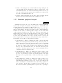
3.17 Runtime graphical output . . . . . . . . . . . . . . . . . . . . . .
33
33
34
4 State
4.1 Population . . . . . . . . . . . . . . . . . .
4.2 Tree depth/size . . . . . . . . . . . . . . . .
4.3 Functions and terminals . . . . . . . . . . .
4.4 Operator probabilities and frequencies . . .
4.5 Population fitness . . . . . . . . . . . . . . .
4.6 Fitness statistics . . . . . . . . . . . . . . .
4.7 Best individual . . . . . . . . . . . . . . . .
4.8 Control . . . . . . . . . . . . . . . . . . . .
4.9 Complexity and diversity statistics/history
.
.
.
.
.
.
.
.
.
.
.
.
.
.
.
.
.
.
.
.
.
.
.
.
.
.
.
.
.
.
.
.
.
.
.
.
.
.
.
.
.
.
.
.
.
.
.
.
.
.
.
.
.
.
.
.
.
.
.
.
.
.
.
.
.
.
.
.
.
.
.
.
.
.
.
.
.
.
.
.
.
.
.
.
.
.
.
.
.
.
.
.
.
.
.
.
.
.
.
.
.
.
.
.
.
.
.
.
38
39
40
41
41
41
42
42
43
43
5 Offline graphical output
5.1 Accuracy versus Complexity
5.2 Pareto front . . . . . . . . .
5.3 Desired versus Obtained . .
5.4 Operator Evolution . . . . .
5.5 Tree visualization . . . . . .
.
.
.
.
.
.
.
.
.
.
.
.
.
.
.
.
.
.
.
.
.
.
.
.
.
.
.
.
.
.
.
.
.
.
.
.
.
.
.
.
.
.
.
.
.
.
.
.
.
.
.
.
.
.
.
.
.
.
.
.
.
.
.
.
.
44
44
44
44
45
45
6 Summary of toolbox functions
6.1 Demonstration functions . . . . . . . . . . .
6.2 Running the algorithm and testing result .
6.3 Parameter and state setting . . . . . . . . .
6.4 Automatic variable checking . . . . . . . . .
6.5 Description of parameter and state variables
6.6 Creation of new generations . . . . . . . . .
6.7 Creation of new individuals . . . . . . . . .
6.8 Filtering of new individuals . . . . . . . . .
6.9 Protected and logical functions . . . . . . .
6.10 Artificial ant functions . . . . . . . . . . . .
6.11 Tree manipulation . . . . . . . . . . . . . .
6.12 Data manipulation . . . . . . . . . . . . . .
6.13 Expected number of children . . . . . . . .
6.14 Sampling . . . . . . . . . . . . . . . . . . .
6.15 Genetic operators . . . . . . . . . . . . . . .
6.16 Fitness . . . . . . . . . . . . . . . . . . . . .
6.17 Diversity measures . . . . . . . . . . . . . .
6.18 Automatic operator probability adaptation
6.19 Runtime graphical output . . . . . . . . . .
6.20 Offline graphical output . . . . . . . . . . .
6.21 Utilitarian functions . . . . . . . . . . . . .
6.22 Text input files . . . . . . . . . . . . . . . .
6.23 License file . . . . . . . . . . . . . . . . . .
.
.
.
.
.
.
.
.
.
.
.
.
.
.
.
.
.
.
.
.
.
.
.
.
.
.
.
.
.
.
.
.
.
.
.
.
.
.
.
.
.
.
.
.
.
.
.
.
.
.
.
.
.
.
.
.
.
.
.
.
.
.
.
.
.
.
.
.
.
.
.
.
.
.
.
.
.
.
.
.
.
.
.
.
.
.
.
.
.
.
.
.
.
.
.
.
.
.
.
.
.
.
.
.
.
.
.
.
.
.
.
.
.
.
.
.
.
.
.
.
.
.
.
.
.
.
.
.
.
.
.
.
.
.
.
.
.
.
.
.
.
.
.
.
.
.
.
.
.
.
.
.
.
.
.
.
.
.
.
.
.
.
.
.
.
.
.
.
.
.
.
.
.
.
.
.
.
.
.
.
.
.
.
.
.
.
.
.
.
.
.
.
.
.
.
.
.
.
.
.
.
.
.
.
.
.
.
.
.
.
.
.
.
.
.
.
.
.
.
.
.
.
.
.
.
.
.
.
.
.
.
.
.
.
.
.
.
.
.
.
.
.
.
.
.
.
.
.
.
.
.
.
.
.
.
.
.
.
.
.
.
.
.
.
.
.
.
.
.
.
.
.
.
.
.
.
48
48
48
48
49
49
49
50
50
50
51
51
51
52
52
52
52
52
53
53
53
53
54
54
.
.
.
.
.
.
.
.
.
.
2
.
.
.
.
.
.
.
.
.
.
.
.
.
.
.
.
.
.
.
.
.
.
.
.
.
.
.
.
.
.
List of Tables
3.1
3.1
3.2
3.2
3.3
3.4
Location of parameters in this manual . . . . . . . .
continued . . . . . . . . . . . . . . . . . . . . . . . .
Possible and default values of the parameters . . . .
continued . . . . . . . . . . . . . . . . . . . . . . . .
Protected and logical functions for use with GPLAB
List of filters for each combination of parameters . .
.
.
.
.
.
.
14
15
16
17
21
25
4.1
4.1
Location of state variables in this manual . . . . . . . . . . . . .
continued . . . . . . . . . . . . . . . . . . . . . . . . . . . . . . .
38
39
3
.
.
.
.
.
.
.
.
.
.
.
.
.
.
.
.
.
.
.
.
.
.
.
.
.
.
.
.
.
.
.
.
.
.
.
.
List of Figures
2.1
Operational structure of the GPLAB toolbox . . . . . . . . . . .
3.1
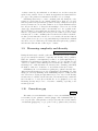
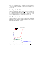
Graphical output produced by the ’plotfitness’ option in the
graphics parameter . . . . . . . . . . . . . . . . . . . . . . . . .
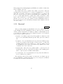
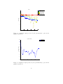
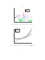
Graphical output produced by the ’plotdiversity’ option in the
graphics parameter . . . . . . . . . . . . . . . . . . . . . . . . .
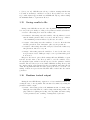
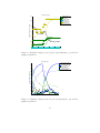
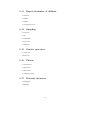
Graphical output produced by the ’plotcomplexity’ option in
the graphics parameter . . . . . . . . . . . . . . . . . . . . . . .
Graphical output produced by the ’plotoperators’ option in the
graphics parameter . . . . . . . . . . . . . . . . . . . . . . . . .
3.2
3.3
3.4
5.1
5.2
5.3
5.4
5.5
Graphical
Graphical
Graphical
Graphical
Graphical
output
output
output
output
output
produced
produced
produced
produced
produced
by
by
by
by
by
the
the
the
the
the
4
function
function
function
function
function
accuracy complexity
plotpareto . . . . .
desired obtained .
operator evolution
drawtree . . . . . .
8
36
36
37
37
45
46
46
47
47
Chapter 1
Introduction
MATLAB [1] is a widely used programming environment available for a large
number of computer platforms. Its programming language is simple and easy
to learn, yet fast and powerful in mathematical calculus. Furthermore, its extensive and straightforward data visualization tools make it a very appealing
programming environment. Toolboxes are collections of optimized, applicationspecific functions, which extend the MATLAB environment and provide a solid
foundation on which to build.
GPLAB is a genetic programming toolbox for MATLAB. Versatile, generalist and easily extendable, it can be used by all types of users, from the layman
to the advanced researcher. It was tested on different MATLAB versions and
computer platforms, and it does not require any additional toolboxes. This
manual is accompanied by a zip file containing all the functions that form the
toolbox, released under GNU General Public Licence. Both are freely available
for download at http://gplab.sourceforge.net/.
Chapter 2 describes the operational structure of GPLAB. Details on the
available parameters and state variables are found in Chaps. 3 and 4 respectively.
Chapter 5 shows the available offline graphical capabilities of GPLAB, and
Chapter 6 presents a summary of all toolbox functions, divided in functional
groups.
1.1
Update from version 2
GPLAB is slowly growing and (hopefully) improving. The changes are always
biased towards my own work, but I also try to incorporate different things
that I have come to realize other users need. Version 2 had already suffered
some updates since its original release: some minor bug fixes and an efficiency
patch, published on the GPLAB website. These introduced modifications to several functions (plotpareto, checkvarsparams, stopcondition, regfitness,
mutation, crossover, maketree), provided a new function (updatenodeids)
and collapsed two functions (findnode, swapnode) into a single one (swapnodes).
5
This new release does not differ much from the previous (updated) one.
Some bugs on the artificial ant problem had been spotted, and another function
(mypower) needed improvement. This new release solves both, and also contains
a simulation function for watching the best ant move on the trail. The main
change in the code is that the artificial ant is now evaluated by its tree, not by
its string. This implied passing the tree as an argument to all the functions that
evaluate an individual (ant or not), and that is why many functions had to be
modified. Here is a list of modified and new functions of this new release:
Modified: demoant, antmove, antleft, antright, antprog2, antprog3,
antif, antfoodahead, antfitness, regfitness, calcfitness, calcpopfitness,
automaticoperatorprobs, stopcondition, intronnodes, dynnodes, dyndepth,
heavydynnodes, heavydyndepth, desired obtained, plotpareto, mypower.
New: anteval, antnewpos, antsim, antpath.
1.2
Acknowledgements
I would like to address a big thank you to Henrik Schumann-Olsen, Jens Thielemann and Oddvar Kloster at SINTEF (http://www.sintef.no) for the extensive additional code they have provided for GPLAB version 1. I have integrated
most of its goodies in version 2, but some are still missing, like the powerful feature of building multiple trees. I intend to integrate it also - no promises when,
though. Thank you so much to Marc Schoenauer’s students Flavien Billard,
Aurlien Boffy, and Thomas De Soza for spotting the nasty artificial ant bugs,
and to Matthew Clifton for the fruitful exchange of ideas and for providing most
of the ant simulation code. Thank you all for providing ideas on how to solve
the bugs, including the people on the MATLAB newsgroup (link). Many other
users have steadily provided a wealth of comments, suggestions and useful code
- thank you all, particularly Mehrashk Meidani, Ali Nazemi, Wo-Chiang Lee,
Vladimir Crnojevic, and Peter J. Acklam. Please forgive me if I have forgotten
someone!
6
Chapter 2
Operational structure
The architecture of GPLAB follows a highly modular and parameterized structure, which different users may use at various levels of depth and insight. What
follows is a visual description of this structure, along with brief explanations
of some operation details and control parameters, algorithm’s variables, a summary of three usage profiles appropriate for different types of users, and details
on how to deal with “plug and play functions”.
2.1
Main modules
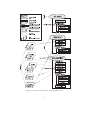
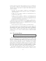
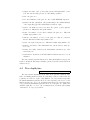
Figure 2.1 shows the operational structure of GPLAB. There are three main
operation modules, namely SET VARS, GEN POP, and GENERATION, and
each represents an interaction point with the user. Inside each main module
the sub-modules are executed from top to bottom, the same happening inside
INITIAL PROBS and ADAPT PROBS. The description of these two can be
found in Sects. 3.13 and 3.12 respectively. Any module with a question mark
can be skipped, depending on the parameter indicated above it. Each module
may use one or more parameters and one or more user functions. User functions
implement alternative or collective procedures for realizing a module, and they
behave as plug and play devices.
2.1.1
GEN POP
This module generates the initial population (INIT POP) and calculates its fitness (FITNESS). The individuals in GPLAB are tree structures initialized with
one of three available initialization methods - Full, Grow, Ramped Half-and-Half
[8]. The functions available to build the trees include the if-then-else statement
and some protected functions, plus any MATLAB function that verifies closure.
The terminals include a random number generator and all the variables necessary, created in runtime. Fitness is, by default, the sum of absolute differences
between the obtained and expected results in all fitness cases. The lower the
7
Figure 2.1: Operational structure of the GPLAB toolbox
8
fitness value, the better the individual. This is the standard for symbolic regression and parity problems (“regfitness” in Fig. 2.1), but GPLAB accepts any
other plug and play function to calculate fitness, like the function for artificial
ant problems, also provided (“antfitness”).
GEN POP is called by the user. It starts by requesting some parameter
initializations to SET VARS, and finishes by passing the execution to GENERATION. If the user only requests the creation of the initial generation, GENERATION is not used.
2.1.2
GENERATION
This module creates a new generation of individuals by applying the genetic
operators to the previous population (OPERATORS). Standard tree crossover
and tree mutation are the two genetic operators available as plug and play
functions. They must have a pool of parents to choose from, created by a SAMPLING method, which may or may not base its choice on the EXPECTED
number of offspring of each individual. Four sampling methods (Roulette [6],
SUS [3], Tournament [4], Lexicographic Parsimony Pressure Tournament [9])
and three methods for calculating the expected number of offspring (Absolute
[7], Rank85 [2], Rank89 [10]) are available as plug and play functions, and any
combination of the two can be used. The genetic operators create new individuals until a new population is filled, a number determined by the generation gap
(see Sect. 3.10).
Calculating fitness is followed by the SURVIVAL module, where the individuals that enter the new generation are chosen according to the elitism level
parameter. The GENERATION module repeats itself until the stop condition
is fulfilled, or when the maximum generation is reached. Several stop conditions
can be used simultaneously (see Sect. 3.14). This module can be called either
by the user or by GEN POP.
2.1.3
SET VARS
This module either initializes the parameters with the default values or updates
them with the user settings. Besides the parameters directly related to the
execution of the algorithm, other parameters affect the output of its results (see
Chap. 3 for a description of all parameters). SET VARS can be called either by
the user or by a request for parameter initialization from GEN POP.
2.2
Working variables
GPLAB uses a vast number of working variables, organized in a structure according to its role in the algorithm. This structure will be referred to as vars
throughout this manual. It is composed of four fields, params, state, pop, data.
Saving vars to a file stores all the information GPLAB uses, produces, and will
ever need to continue a previously started run.
9
• params stores all the variables that determine different ways of running
the different parts of the algorithm. These are settings that are not supposed to vary during the course of a run, although the user can continue
a GPLAB run with a different set of parameters from how it started.
Chapter 3 is dedicated to the different running aspects of GPLAB - each
subsection refers to one or more parameters related to that aspect.
• state stores all the variables that represent the current state of the algorithm. These settings are constantly updated during the run, and should
not be modified by the user. Chapter 4 is dedicated to describing the
meaning of the various state variables.
• pop stores the current population. This variable is constantly updated
as the population evolves. It can be considered a state variable and,
accordingly, its description can be found in Chap. 4.
• data is the data set(s) used by the algorithm to guide the evolutionary
process and, optionally, perform cross-validation, imported from files in
the beginning of each run. Because it is stored along with the other
algorithm’s variables, continuing a previously started run does not require
the user to provide the data files again.
2.3
Usage
The large amount of available control parameters may lead to the wrong conclusion that it will take a long time before one can start using the toolbox
comfortably, and that only expert users will ever be able to use it properly. On
the contrary, GPLAB is very easy to use and suits even the unknowledgeable
users, due to the automatic parametrization of most parameters. Here is a summary of three different profiles of usage that may be given by different types of
users: the layman, the regular user, and the advanced researcher.
2.3.1
The layman
This user wants to try a genetic programming algorithm to achieve a solution
to a standard problem, without having to learn about available parameters, or
how to set them. The available functions are
[vars,b]=gplab(g,n);
[vars,b]=gplab(g,vars);
where g is the maximum number of generations to run the algorithm and n is
the population size.
The first function initializes all the parameters of the algorithm with the
default values and runs it for g generations with n individuals. The user will be
asked about the location of the data files to use (see Sect. 3.8). It returns vars,
all the variables of the algorithm, and b, the best individual found, which is the
10
same as vars.state.bestsofar. The second function continues a previously
started run for another g generations, and also needs vars as an input argument. These two functions correspond to the operation modules GEN POP and
GENERATION shown in Fig. 2.1.
GPLAB also provides some demonstration functions to illustrate its usage
in different types of problems (see Chap. 6 for a complete list of functions):
• demo - runs a symbolic regression problem (the quartic polynomial) with
50 individuals for 25 generations, with automatic adaptation of operator
probabilities, and performing cross-validation in a different data set (the
exponential). It draws all the available plots in runtime (see Sect. 6.19),
and finishes with several additional output plots (see Sect. 5), including
the pareto front and the drawing of the best individual found.
• demoparity - runs the parity-3 problem with 50 individuals for 20 generations, with fixed operator probabilities, drawing some of the available
runtime plots, and finishing by drawing the best individual found.
• demoant - runs the artificial ant problem in the Santa Fe food trail with
20 individuals for 10 generations, drawing half of the available plots in
runtime, and finishing by drawing the best individual found.
2.3.2
The regular user
This is the type of user who knows what the parameters mean and wants to test
different sets of values besides the defaults. To set the parameters the available
functions are
params=resetparams;
params=setparams(params,’param1=value1,param2=value2,etc’);
[vars,b]=gplab(g,n,params);
where param1, param2 are the names of parameters, and value1, value2 the
values pretended.
The first function initializes and returns the parameters structured variable
with the default values, and the second alters some of the parameters according
to the list given as argument. The third acts like the first function described
for the layman, except that it uses the parameter values previously set instead
of initializing them with the default values. The parameter setting functions
correspond to the module SET VARS in Fig. 2.1. resetparams is appropriate
for symbolic regression problems. For different types of problems, one should see
the parameter settings used on the demo functions demoparity and demoant.
Please see Chap. 6 for a complete list of functions. There are also functions
dedicated to setting some specific parameters, like the genetic operators, and
the functions and terminals used to build the trees (see Sects. 3.4 and 3.3 for
details).
11
2.3.3
The advanced researcher
Here is the user who wants to build and test new sampling methods, new genetic
operators, in short, new user functions as shown in Fig. 2.1, without having
to construct a new toolbox from the beginning. GPLAB allows this with a
minimum amount of effort, thanks to its plug and play operational structure.
As an example, the user who wants to test a new genetic operator only has to
build a new function that implements it, using the tree manipulation functions
provided. This function should use the same input and output arguments as
the other genetic operators (a template for building new genetic operators is
provided in Sect. 3.4). To tell the algorithm about the new genetic operator the
available function is
params=addoperators(params,’newoperator’,nparents,nchildren);
where newoperator is the name of the new function, nparents is the number
of parents the new operator needs, and nchildren is the number of offspring
it produces. Details on how to build new plug and play user functions can be
found in Chap. 3 (please search for the particular subsection that applies) and
the way to integrate them into GPLAB is described in Sect. 2.4.
2.4
Plug and play
Figure 2.1 shows that most modules of the GPLAB operational structure are
based on a set of user functions that act as plug and play devices. There are
three important aspects related to these functions: how to build them, how to
use them, and how to integrate them in GPLAB.
2.4.1
Building plug and play functions
Building a new plug and play function is like building any other MATLAB
function while following the rules pertaining input and output arguments. Each
module defines its own set of input and output arguments, so the interested user
should refer to the appropriate section in Chap. 3.
2.4.2
Using new plug and play functions
To use a newly built plug and play function, the user must declare its existence in
the algorithm’s parameters. Once again, each module is associated to different
parameter variables, and the user should refer to the appropriate section in
Chap. 3, but the general form of doing this is
vars.params.<specificvariable>=’name_new_func’;
where <specificvariable> is the parameter that refers to the module adopting
the new function. This may look equivalent to doing
params=setparams(params,’<specificvariable>=name_new_func’);
12
but this form of setting parameters will be refused for the new plug and play
function until it is fully integrated as part of GPLAB.
2.4.3
Integrating new plug and play functions in GPLAB
Integrating a new function in GPLAB is done by editing the toolbox file availableparams. This file contains the declarations of the fields that constitute the
structure variable params, as well as their possible and default values - where
the possible values may be the names of the plug and play functions. This file
is divided in three parts: the first specifies which variables form the structure
params; the second specifies the possible values for each variable; the third
specifies the default values for each variable. As an example, to integrate a
new plug and play function called ’newfitness’ that implements a new way of
measuring fitness, a new line should be added:
myparams.calcfitness={’regfitness’,’antfitness’,’newfitness’};
where ’regfitness’ and ’antfitness’ are the standard procedures for calculating fitness already provided by GPLAB. This line tells GPLAB that all three
procedures can be used for calculating fitness. When the algorithm begins,
’regfitness’ is still the default fitness procedure, but the user can change it
before starting the run. Because ’newfitness’ is already declared as a standard
GPLAB function, this change can be made with the setparams function:
params=setparams(params,’calcfitness=newfitness’);
To make ’newfitness’ the default procedure without the need to change the
setting before running the algorithm, the line
defaults.calcfitness=’’’regfitness’’’;
in the availableparams file should be replaced with
defaults.calcfitness=’’’newfitness’’’;
Names of functions have to be accompanied by the triple “’”, but numeric
settings can be made like in this example:
defaults.hits=’[100 0; 90 10]’;
The exceptions to the description above are all the cases when the new plug
and play function is to be used along with other plug and play functions,
like the genetic operators and the functions and terminals. Please see file
availableparams for examples.
Similarly, the file availablestates may also be edited to include new fields
in the structure variable state. This may have to be done if a new plug and play
function intends to use state variables other than the ones available. This is an
advanced action that should not be attempted without proper care.
13
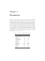
Chapter 3
Parameters
The next sections describe aspects related to the parameters used by GPLAB what are the parameters involved in each part of the algorithm, and how their
modification affects its behavior. Each subsection concerns one or more parameter variables, and each parameters may appear in more than one subsection.
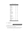
Table 3.1 indicates the location of each parameter in this manual, and Table 3.2
specifies their possible and default values. When setting parameters, using the
function setparams will ensure minimum range checking, whereas setting the
fields of the variable vars.params directly will not. Some parameter settings
are automatically corrected to allowed values (with a warning to the user) in
case they are set incorrectly. Others are automatically set when left empty.
Generally speaking, the only parameters that must be set by the user are the
maximum number of generations, the population size, and the names of the files
that contain the data set (see Sect. 2.3).
Table 3.1: Location of parameters in this manual
Parameter
adaptinterval
adaptwindowsize
autovars
calccomplexity
calcdiversity
calcfitness
datafilex
datafiley
depthnodes
dynamiclevel
expected
files2data
filters
Section
Page
3.12
31
3.12
31
3.3
19
3.9
29
3.9
29
3.8
27
3.8
27
3.8
27
3.1,3.2,3.5 17,18,24
3.2,3.5
18,24
3.7
26
3.8
27
3.5
24
continued on next page
14
Table 3.1: continued
Parameter
fixedlevel
functions
gengap
graphics
hits
inicdynlevel
inicmaxlevel
initialfixedprobs
initialprobstype
initialvarprobs
initpoptype
keepevalssize
lowerisbetter
minprob
numbackgen
numvars
operatornames
operatornchildren
operatornparents
operatorprobstype
output
percentback
percentchange
precision
realmaxlevel
reproduction
sampling
savedir
savetofile
smalldifference
survival
terminals
testdatafilex
testdatafiley
tournamentsize
usetestdata
Section
3.2,3.5
3.3
3.10
3.17
3.14
3.2
3.1
3.13
3.13
3.13
3.1
3.8
3.8
3.12
3.12
3.3
3.4
3.4
3.4
3.12
3.16
3.12
3.12
3.8
3.2
3.4
3.6
3.15
3.15
3.13
3.11
3.3
3.8
3.8
3.6
3.8
15
Page
18,24
19
29
34
32
18
17
32
32
32
17
27
27
31
31
19
22
22
22
31
33
31
31
27
18
22
25
33
33
32
30
19
27
27
25
27
Table 3.2: Possible and default values of the parameters
Parameter
adaptinterval
adaptwindowsize
autovars
calccomplexity
fixedlevel
Possible values
integer ≥ 0
integer ≥ 0
’0’,’1’
’0’,’1’
(list of diversity measures,
see Sect. 3.9)
’regfitness’,’antfitness’
(name of a valid input file)
(name of a valid input file)
’1’,’2’
’0’,’1’,’2’
’absolute’,’rank85’,’rank89’
’xy2inout’,’anttrail’
(list of filter functions,
see Sect. 3.5)
’0’,’1’
functions
(see Sect. 3.3)
calcdiversity
calcfitness
datafilex
datafiley
depthnodes
dynamiclevel
expected
files2data
filters
gengap
graphics
hits
integer> 0
(list of plot names,
see Sect. 3.17)
(list of stop conditions,
see Sect. 3.14)
inicdynlevel
integer> 0
inicmaxlevel
integer> 0
(list of probability values)
’fixed’,’variable’
(list of probability values)
’fullinit’,’growinit’,’rampedinit’
integer≥ 0
0,1
> 0 and ≤ 1
integer> 0
[ ] or integer≥ 0
(list of operator names,
operatornames
see Sect. 3.4)
operatornchildren (list of number of children produced)
operatornparents
(list of number of parents needed)
operatorprobstype
’fixed’,’variable’
output
’silent’,’normal’,’verbose’
percentback
≥ 0 and ≤ 1
percentchange
> 0 and ≤ 1
precision
integer> 0
initialfixedprobs
initialprobstype
initialvarprobs
initpoptype
keepevalssize
lowerisbetter
minprob
numbackgen
numvars
realmaxlevel
integer> 0
reproduction
≥ 0 and < 1
’roulette’,’sus’,
’tournament’,’lexictour’
(name for a new directory)
sampling
savedir
16
Default value
[ ], see Sect. 6.18
[ ], see Sect. 6.18
’1’
’0’
{ }
’regfitness’
(user provided, see Sect. 3.8)
(user provided, see Sect. 3.8)
’1’
’1’
’rank85’
’xy2inout’
{ }
’1’
’plus’,’minus’,’times’,
’sin’, ’cos’,’mylog’
[ ], see Sect. 3.10
{ }
[100, 0]
6 if depthnodes=’1’
28 if depthnodes=’2’
6 if depthnodes=’1’
28 if depthnodes=’2’
[ ], see Sect. 3.13
’fixed’
[ ], see Sect. 3.13
’rampedinit’
[ ], see Sect. 3.8
1
0.1
3
[ ], see Sect. 3.3
{’crossover’,’mutation’}
[2,1]
[2,1]
’fixed’
’normal’
0.25
0.25
12
17 if depthnodes=’1’
512 if depthnodes=’2’
0.1
’lexictour’
(user provided, see Sect. 3.15)
continued on next page
Table 3.2: continued
Parameter
savetofile
smalldifference
survival
terminals
testdatafilex
testdatafiley
tournamentsize
usetestdata
3.1
Possible values
’never’,’firstlast’,
’every10’,’every100’,’always’
> 0 and ≤ 1
’replace’,’keepbest’,
’halfelitism’,’totalelitism’
(see Sect. 3.3)
(name of a valid input file)
(name of a valid input file)
[ ] or > 0 (integer if ≥ 1)
0,1
Default value
’never’
[ ], see Sect. 3.13
’replace’
{}
(user provided, see Sect. 3.8)
(user provided, see Sect. 3.8)
[ ], see Sect. 3.6
0
Tree initialization
inicmaxlevel,depthnodes,initpoptype
The initial population of trees, created in runtime in the beginning of a GPLAB
run, is done by choosing random functions and terminals from the respective
sets (Sect. 3.3). The initial maximum depth/size of the new trees, determined
by the parameter inicmaxlevel, must not be violated, but besides this rule
there is still room for different options that may influence the structure of the
initial trees. These options constitute what is called the generative method,
specified by the parameter initpoptype. There are three different methods
available in GPLAB, used in the plug and play fashion described in Sect. 2.4,
and each of them uses either the standard procedure based on depth [8], or
the new variation based on size, i.e., number of nodes [12], depending on the
parameter depthnodes (’1’ for depth, ’2’ for size, see Sect. 3.2):
• ’fullinit’ - this is the Full method. In the standard procedure, the
new tree receives non terminal (internal) nodes until the initial tree depth
(inicmaxlevel parameter) is reached - the last depth level is limited to
terminal nodes. As a result, trees initialized with this method will be
perfectly balanced with all the branches of the same length.
If size is used instead of depth, internal nodes are chosen until the size of
the new tree is close to the specified size (inicmaxlevel), and only then
terminals are chosen. Unlike the standard procedure, the size variation
may not be able to create trees with the exact size specified, but only close
(never exceeding).
• ’growinit’ - this is the Grow method. In the standard procedure, each
new node is randomly chosen between terminals and non terminals, except
nodes at the initial tree depth level, which must be terminals. Trees
created with this method may be very unbalanced, with some branches
much longer than others, and their depth may be anywhere from 1 to the
value of the inicmaxlevel parameter.
17
If using the size variation, nodes are also chosen randomly, but prior to
reaching the size specified in inicmaxlevel, care is taken on the choice
on the internal nodes, based on their arity, so as to guarantee the inicmaxlevel will not be exceeded by the respective arguments (which now
have to be terminals).
• ’rampedinit’ - this is the Ramped Half-and-Half method. In the standard
procedure, an equal number of individuals are initialized for each depth
between 2 and the initial tree depth value. For each depth level considered,
half of the individuals are initialized using the Full method, and the other
half using the Grow method. The population of trees resulting from this
initialization method is very diverse, with balanced and unbalanced trees
of several different depths.
In the size variation, an equal number of individuals are initialized with
sizes ranging from 2 to inicmaxlevel. As in the standard procedure, for
each size, half of the trees are initialized with the Full method, and the
other half with the Grow method.
3.2
Tree depth and size limits
fixedlevel,realmaxlevel,dynamiclevel,inicdynlevel,depthnodes
Trees in GPLAB may be subject to a set of restrictions on depth or size (number
of nodes), by setting appropriate parameters. These restrictions are meant
to avoid bloat, a phenomenon consisting of an excessive code growth without
the corresponding improvement in fitness. The standard way of avoiding bloat
is by setting a maximum depth on trees being evolved - whenever a genetic
operator produces a tree that breaks this limit, one of its parents enters the
new population instead [8].
GPLAB implements this strict limit on depth, as well as a dynamic limit,
similar to the first, but with two important differences: it is initially set with
a low value; it is increased when needed to accommodate an individual that
is deeper than the dynamic limit but is better than any other individual found
during the run. Both limits can be used in conjunction. For each new individual
produced by a genetic operator there are three possible scenarios:
– The individual does not exceed the dynamic maximum depth - it can be
used freely because no constraints have been violated.
– The individual is deeper than the dynamic maximum depth, but does not
exceed the strict maximum depth stored in realmaxlevel - its fitness is
measured. If the individual proves to be better than the best individual
found so far, the dynamic maximum depth is increased and the new individual is allowed into the population; otherwise, the new individual is
rejected and one of its parents enters the population instead.
18
– The individual is deeper than the strict maximum depth stored in realmaxlevel - it is rejected and one of its parents enters the population
instead.
The dynamic maximum tree depth technique is a recent technique that
has shown to effectively control bloat in two different types of problems (see
[11] for details). The parameter dynamiclevel can be used to turn it on
(dynamiclevel=’1’, the default) or off (dynamiclevel=’0’). When on, its
initial value is determined by the parameter inicdynlevel. This should not be
confounded with the maximum depth of the initial random trees, inicmaxlevel
(see Sect. 3.1). The strict depth limit can also be turned on (fixedlevel=’1’)
or off (fixedlevel=’0’). When on, the strict maximum depth of trees is determined by the parameter realmaxlevel.
Even more recently, two variations on the dynamic limit technique have been
introduced: a heavy dynamic limit (dynamiclevel=’2’), where the dynamic
limit can (unlike the original one) fall back to a lower value in case the new best
individual allows it, and the dynamic limit on size (number of nodes), regardless
of depth (see [12] for details). The parameter depthnodes is used to switch
between depth (depthnodes=’1’) and size (depthnodes=’2’) restrictions. Any
combination of fixedlevel, dynamiclevel and depthnodes can be used. The
default initial values for realmaxlevel and inicdynlevel depend on the setting
of depthnodes (see Table 3.2).
The dynamic limits are turned on in the demo functions of the toolbox, and
the (original) dynamic limit on depth is even used as default, along with the
strict limit, because this combination seems to be very effective in controlling
bloat. Nevertheless, the user should keep in mind that they are still experimental
techniques.
3.3
Functions and terminals
functions,terminals,numvars,autovars
As any genetic programming algorithm, GPLAB needs functions and terminals
to create the population, in this case the parse trees that represent individuals.
Functions GPLAB can use any MATLAB function that verifies closure, plus
some protected and logical functions and the if-then-else statement, also available as part of the toolbox. The user indicates which functions the algorithm
should use by setting the parameter variable functions. Table 3.3 contains
information on the available toolbox functions.
All the functions described in Table 3.3 are used in the plug and play fashion described in Sect. 2.4. The advanced users who want to build and use
their own functions only have to implement them as MATLAB functions (and
make sure the input arguments can be either scalars or vectors – see MATLAB
user’s manual) and declare them using one of the toolbox functions (use “help
setfunctions” and “help addfunctions” in the MATLAB prompt for usage):
19
params=setfunctions(params,’func1’,2,’func2’,1);
params=addfunctions(params,’func1’,2,’func2’,1);
setfunctions defines the set of available functions as containing functions
’func1’ and ’func2’, replacing any other functions previously declared. ’func1’
has arity 2 - it needs two input arguments; ’func2’ has arity 1. Any number of functions can be declared at one time, by adding more arguments to
setfunctions. addfunctions accepts the same arguments but adds the declared functions to the already defined set, keeping the previously declared
functions untouched. setfunctions and addfunctions are friendly substitutes
to directly setting the parameter variable functions. The declaration of genetic
operators is done similarly (see Sect. 3.4).
Some examples of MATLAB functions that verify closure, fit for use with
GPLAB:
• plus, minus, times
• sin, cos
• and, or, not, xor
• ceil, floor
• min, max
• eq (equal), gt (greater than), le (less than or equal)
GPLAB also includes some functions for artificial ant problems, namely
antif, antprogn2, antprogn3, arities 2, 2, 3 respectively.
Terminals GPLAB can use any constant as a terminal, plus a random number
between 0 and 1, generated in runtime, as the function ’rand’ with null arity.
The declaration of terminals is done similarly to the declaration of functions, by
using friendly substitutes to directly setting the parameter variable terminals.
For example, to declare the constant ’1’ and the random number generator
as members of the set of terminals (use “help setterminals” in the MATLAB
prompt for usage):
params=setterminals(params,’rand’,’1’);
Unlike in setfunctions, there is no need to indicate the arity, which is always
null. To add a new terminal to an already declared set of terminals (use “help
addterminals” in the MATLAB prompt for usage):
params=addterminals(params,’new_terminal’);
Any number of terminals can be declared or added at one time, by adding
more input arguments. The terminals available for artificial ant problems are
antright, antleft, antmove.
20
Table 3.3: Protected and logical functions for use with GPLAB
Protected
function
Division
Square root
Power
Natural
logarithm
Base 2
logarithm
Base 10
logarithm
If-then-else
statement
Negation of
AND
Negation of
OR
MATLAB
Input
Output argument1
function arguments
a (if b = 0)
mydivide
a, b
a/b (otherwise)
0 (if a <= 0)
mysqrt
a
sqrt(a) (otherwise)
ab (if ab is a valid non-complex number)
mypower
a, b
0 (otherwise)
0 (if a = 0)
mylog
a
log(abs(a)) (otherwise)
0 (if a = 0)
mylog2
a
log2(abs(a)) (otherwise)
0 (if a = 0)
mylog10
a
log10(abs(a)) (otherwise)
eval(c) (if eval(a)= 0)
myif
a, b, c
eval(b) (otherwise)
nand
a, b
not(and(a, b))
nor
a, b
not(or(a, b))
1
sqrt,log,log2,log10,abs,eval,not,and,or are MATLAB functions.
eval(x) returns the result of evaluating the expression x.
21
Variables needed to evaluate the fitness cases are also part of the set of available terminals for the algorithm to work with, and these can only be generated
(automatically) in the beginning of the run, according to the settings of the
parameters numvars and autovars:
• numvars=[] and autovars=’0’ - the parameter numvars is automatically
filled with 0 and no variables are generated. This setting is appropriate
for artificial ant problems.
• numvars=[] and autovars=’1’ - the parameter numvars is automatically
filled with the number of columns of the input data set and these many
variables are generated. This setting is appropriate for symbolic regression
and parity problems.
• numvars=x - customized setting, where x is the number of variables generated, corresponding to the x first columns of the input data set.
3.4
Genetic operators
reproduction,operatornames,operatornparents,operatornchildren
GPLAB may use any number of genetic operators to create new individuals.
A proportion of individuals, specified in parameter reproduction, may also be
copied into the next generation without suffering the action of the operators.
Tree crossover and tree mutation are the genetic operators provided by
GPLAB, implemented as follows:
Crossover In tree crossover, random nodes are chosen from both parent trees,
and the respective branches are swapped creating two offspring. There is no bias
towards choosing internal or terminal nodes as the crossing sites.
Mutation In tree mutation, a random node is chosen from the parent tree
and substituted by a new random tree created with the terminals and functions
available. This new random tree is created with the Grow initialization method
and obeys the size/depth restrictions imposed on the trees created for the initial
generation (see Sect. 3.1).
Although these are the only genetic operators provided, the addition of others is straightforward, thanks to the modular structure shown in Fig. 2.1. A new
genetic operator is simply a MATLAB function used as a plug and play device
to module OPERATOR, and the declaration of its existence to the algorithm
is made similarly to the setting of functions and terminals (see Sect. 3.3), with
one of the toolbox functions (use “help setoperators” and “help addoperators”
in the MATLAB prompt for usage):
params=setoperators(params,’operator1’,2,2,’operator2’,2,1);
params=addoperators(params,’operator1’,2,2,’operator2’,2,1);
22
The first function defines the set of genetic operators as containing operators ’operator1’ and ’operator2’, replacing any operator previously declared.
’operator1’ needs two parents and produces two children; ’operator2’ also
needs two parents but produces only one child. Any number of genetic operators can be declared at one time, by adding more arguments to the function. The
second function accepts the same arguments but adds the declared operators to
the already defined set, keeping the previously declared operators untouched.
These functions have the same effect as directly setting the parameter variables
operatornames, operatornparents, operatornchildren.
’operator1’ and ’operator2’ are the names of the new MATLAB functions
that implement the new operators. The only rules these functions must follow
concern their input and output arguments. Please see functions crossover and
mutation for examples on how to correctly build genetic operators. A set of
tree manipulation functions is available (use “help <function name>” in the
MATLAB prompt for usage):
• maketree(level,functions,arities,exactlevel,depthnodes) – this
function returns a new random tree no deeper/bigger than level, using the functions with respective arities. If exactlevel is true, the
new tree will be initialized using the Full method; otherwise, it will be
initialized using the Grow method (see Sect. 3.1). depthnodes indicates
whether restrictions are to be applied in tree depth or tree size (number
of nodes)
• tree2str(tree) – returns the string that tree represents
• findnode(tree,x) – returns the subtree of tree with root on node number x. The nodes are numbered depth-first
• swapnode(tree,x,node) – returns the result of swapping node number x
in tree for node
• tree2str(tree) – returns the translation of tree into a string
• treelevel(tree) – returns the depth of tree
• nodes(tree) – returns the number of nodes of tree
• intronnodes(tree,params,data,state) – returns the number of introns
of tree. Needs the variables params, data and state.
Unlike in previous versions of GPLAB, the genetic operators do not need to
return offspring that conform to the tree depth/size restrictiona being applied
(see Sect. 3.2) - this is now performed afterwards by applying validation (also
called filter) functions (see Sect. 3.5).
Of all the fields an individual contains, only origin, parents, tree and
str must be filled. id should be left empty ([]) to be filled by the validation
functions mentioned above. All the other fields (xsites, fitness, result, testfitness, nodes, introns, level) can also be left empty if not needed by the genetic
23
operator, because they will be calculated and stored as needed by other procedures. xsites is the exception - as a merely informative field, that may contain
information concerning the nodes where the parent trees were split to create
the child tree, if left empty it will remain so, as no other other function in the
current version of GPLAB uses it.
3.5
Validating new individuals
filters,fixedlevel,dynamiclevel,depthnodes
After a new individual is produced by any of the genetic operators, it must
be validated in terms of depth/size before being considered as a candidate for
the new population. Several validation functions, or filters, are provided in
GPLAB, and others may be built and integrated as plug and play functions
(see Sect. 2.4). The filters parameter is simply a list of those functions, by
the order in which they should be applied. It should not, however, be set by the
user, but instead be automatically set, in the beginning of the run, depending
on the parameters fixedlevel, dynamiclevel and depthnodes. Bellow is a
list of available filter functions along with the description of their purpose (see
Sect. 3.2 for more details):
• ’strictdepth’ - this filter rejects an individual that is deeper than the
strict maximum allowed depth; does nothing otherwise.
• ’strictnodes’ - this filter rejects an individual that is bigger (contains
more nodes) than the strict maximum allowed size; does nothing otherwise.
• ’dyndepth’ - this filter measures the fitness of an individual that is deeper
than the dynamic maximum allowed depth: if the individual is better than
the best so far, the dynamic depth is increased and the new individual is
accepted; otherwise it is rejected. The filter does nothing if the individual
is no deeper than the limit.
• ’dynnodes’ - the same as the previous one, but considering size (number
of nodes) instead of depth.
• ’heavydyndepth’ - this filter measures the fitness of an individual and
checks its depth. If it is deeper than the dynamic maximum allowed
depth: if the individual is better than the best so far, or if it is no deeper
than the deepest of its parents, the filter increases the dynamic depth if
needed and accepts the individual, otherwise rejects it. If the individual
is less deep than the dynamic maximum allowed depth: if it is the better
than the best so far, the filter accepts it and lowers the dynamic depth,
and does nothing otherwise.
• ’heavydynnodes’ - the same as the previous one, but considering size
(number of nodes) instead of depth.
24
Table 3.4: List of filters for each combination of parameters
Filters list
fixedlevel
dynamiclevel
depthnodes
{ }
{’dyndepth’}
{’dynnodes’}
{’heavydyndepth’}
{’heavydynnodes’}
{’strictdepth’}
{’strictnodes’}
{’strictdepth’,’dyndepth’}
{’strictnodes’,’dynnodes’}
{’strictdepth’,’heavydyndepth’}
{’strictnodes’,’heavydynnodes’}
0
0
0
0
0
1
1
1
1
1
1
0
1
1
2
2
0
0
1
1
2
2
1
2
1
2
1
2
1
2
1
2
The above filters may reject an individual, accept an individual, or do neither. After passing through all the filters, the individuals that still haven’t
been rejected or accepted will finally be accepted as candidates for the new
population.
Table 3.4 lists the appropriate list of filters for each combination of the
3 depth/size related parameters (fixedlevel, dynamiclevel, depthnodes).
Once again, the list of filters is chosen automatically by GPLAB in the beginning of the run.
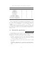
3.6
Selection for reproduction
sampling,tournamentsize
As shown in Fig. 2.1, genetic operators need parent individuals to produce
their children. In GPLAB these parents are selected according to one of four
sampling methods, as indicated in the parameter variable sampling:
• ’roulette’ - this method acts as if a roulette with random pointers is
spun, and each individual owns a portion of the roulette that corresponds
to its expected number of children (see Sect. 3.7).
• ’sus’ - this method also relies on the roulette, but the pointers are equally
spaced [3].
• ’tournament’ - this method chooses each parent by randomly drawing a
number of individuals from the population and selecting only the best of
them.
25
• ’lexictour’ - this method implements lexicographic parsimony pressure
[9]. Like in ’tournament’, a random number of individuals are chosen from
the population and the best of them is chosen. The main difference is, if
two individuals are equally fit, the shortest one (the tree with less nodes)
is chosen as the best. This technique has shown to effectively control bloat
in different types of problems (see [9] for details).
When either of the tournament methods is chosen, the number of individuals
participating in each tournament is determined by the parameter variable tournamentsize. Like gengap (see Sect. 3.10), the value of this parameter can
represent either the absolute number of individuals (tournamentsize>=1), or a
proportion of the population size (otherwise). When the tournament method is
chosen and tournamentsize is left blank (tournamentsize=[]), GPLAB sets
it with the default value (10% of the population size or 2, which one is larger) in
the beginning of the run. If tournamentsize equals 1, the selection of parents is
random; if tournamentsize equals the population size, only the best individual
in the population is chosen to produce all the offspring. The tournament method
does not need to know the expected number of children of each individual, unlike
the other two methods.
Alternative sampling methods may be built and easily used in GPLAB, as
plug and play devices to module SAMPLING (see Fig. 2.1). All the user has
to do is build a new function that implements the sampling method, respecting
the input and output arguments, and set the parameter variable sampling with
the name of the new function:
params.sampling=’new_sampling_method’;
The new function must accept as input arguments the current population, parameters and state (vars.pop, vars.params, vars.state), the number of individuals to draw, and a list of identifiers of individuals that must not be drawn.
This last input argument is not being used in the current version of GPLAB,
but the available sampling procedures contemplate this possibility. The function
must output the identifiers of the parents chosen, their indices in the current
population, the expected number of children of all individuals in the population, and the normalized fitness of all individuals in the population. The last
two output arguments may be left blank ([]) if the sampling procedure does
not calculate them. Please see functions roulette, sus and tournament for a
prototype.
3.7
Expected number of children
expected
As described in Sect. 3.6, some sampling procedures choose the parents based
on their expected number of children, while others only need to know which are
better than which. Likewise, the calculation of the expected number of children
may use the actual fitness values, or simply their rank in the population. The
26
parameter variable expected determines with method is used for calculating the
expected number of children for each individual. This calculation is performed
only if the selection for reproduction so requires. Three different methods are
available in GPLAB:
• ’absolute’ - the expected number of children for each individual is proportional to its absolute fitness value (it is equal to its normalized, or
relative, fitness) [7].
• ’rank85’ - the expected number of children for each individual is based on
its rank in the population [2].
• ’rank89’ - the expected number of children for each individual is based
on its rank in the population and on the state of the algorithm (how far
it is from the maximum allowed generation). The differentiation between
individuals increases in later generations [10].
Alternative methods for calculating the expected number of children may be
built and used as plug and play devices to module EXPECTED (see Fig. 2.1),
by simply implementing the new method in a MATLAB function and declaring
it in the parameter variable expected:
params.expected=’new_expected_number_of_children_method’;
The new function must accept as input arguments the current population and
state (vars.pop, vars.state), and output the expected number of children of
all individuals in the population, and the normalized fitness of all individuals
in the population. The last output argument may be left blank ([]) if its
calculation is not needed. Please see functions absolute, rank85 and rank89
for a prototype.
3.8
Measuring fitness
files2data,datafilex,datafiley,testdatafilex,testdatafiley
usetestdata,calcfitness,precision,lowerisbetter,keepevalssize
When starting a GPLAB run the user is required to indicate the names of the
files where the fitness cases are stored. The files should be in a format readily
importable to MATLAB, like Tab delimited text. For symbolic regression and
parity problems, the first file should contain the input values, and the second the
expected - or desired - output value, one row for each fitness case. For artificial
ant problems, the first file should contain the food trail, in the form of a binary
matrix, and the second file should contain the number of food pellets in it. After
importing the data stored in these files to the algorithm’s variables, according to
the procedure specified in the parameter files2data, GPLAB saves its names
with complete path in the parameter variables datafilex and datafiley.
The parameter usetestdata may be used to indicate whether the best individual found so far should have its fitness measured in a different data set
27
(usetestdata=1) or not (usetestdata=0). If yes, this extra measurement will
be done in every generation, and the user must provide the names of the two
(input and desired output) extra data files, to be stored in testdatafilex and
testdatafiley. When restarting a run, the user does not have to provide any
file names again.
Two different methods for importing the text files into the algorithm’s variables are available in GPLAB (not shown in Fig. 2.1):
• ’xy2inout’ - for symbolic regression and parity problems.
• ’anttrail’ - for artificial ant problems.
Accordingly, there are also two methods for calculating fitness in GPLAB, implemented as plug and play functions (see Fig. 2.1):
• ’regfitness’ - calculates, for each individual, the sum of the absolute
difference between the expected output value and the value returned by
the individual on all fitness cases. The best individuals are the ones that
return values less different than the expected values - the ones with a lower
fitness. This function should be used with the parameter lowerisbetter
set to ’1’.
• ’antfitness’ - calculates, for each individual, the number of food pellets
eaten in the artificial ant food trail during 400 time steps - the best individuals are the ones who eat more pellets, meaning they have higher
fitness. This function should be used with the parameter lowerisbetter
set to ’0’.
When regfitness is used, all the fitness values stored in the algorithm’s variables are rounded to a certain number of decimal places, given by the parameter
precision. This is meant to avoid rounding errors that affect the comparison
of two different individuals who have the same fitness. For example, in symbolic regression problems, it is common to see individuals with fitness values
like 5.9674e-016 and 1.0131e-015. Without using the precision parameter,
the first individual would be chosen as the best, even when the second one is
smaller, because these two values are not the same - just because of the rounding
error, since they are in fact both null. By default, precision is set to 12, but
the user can give it any integer number higher that 0.
To use an alternative method for calculating fitness, all the user has to do is
build a new function, respecting the input and output arguments, and set the
parameter variable calcfitness with the name of the new function:
params.calcfitness=’new_calcfitness_method’;
The new function must accept as input arguments the string expression of
the individual to measure (vars.pop(i).str), the parameters (vars.params),
the data variable (vars.data), the terminals (vars.state.terminals) and the
varsvals string (see Sect. 4.5) containing all the fitness cases in a format ready
for assignment; it must output the fitness value of the individual, the vector
28
of values returned by the individual on each fitness case, and if necessary the
updated state variable. Please see functions regfitness and antfitness for
prototypes. The parameter lowerisbetter should be set accordingly.
Calculating fitness may be a time consuming task, and during the evolutionary process the same tree is certainly evaluated more than once. To avoid
this, the parameter keepevalssize specifies how many evaluations are kept in
memory for future use, in case their results are needed again. Evaluations used
less often are the first to be discarded when making room for new ones. If left
empty ([]), keepevalssize will be automatically set to the population size.
The ideal balance between CPU time and memory is not easy to find, and one
must not forget that searching the memory for the results of previous evaluations may also be a time consuming task. Nevertheless, it is almost essential to
use this option in runs where the user chooses to measure the amount of introns
of the generated trees (see Sect. 3.9), particularly in problems like the artificial
ant, where every tree branch is repeated many times throughout the population,
and takes the same amount of time steps to evaluate.
3.9
Measuring complexity and diversity
calccomplexity,calcdiversity
During the run it may be useful to gather more information about the evolutionary process, namely the structure, complexity and diversity of the population.
When the parameter calccomplexity is turned on (calccomplexity=’1’),
GPLAB stores information regarding the number of nodes and intron nodes
of the trees, depth level and balancing between branches (tree fill rate, see [12]).
Obtaining some of this information is extremely time consuming, particularly
the number of introns, so it must not be used unless absolutely necessary.
GPLAB may also store information regarding the population diversity. Two
different diversity measures are provided (’uniquegen’ and ’hamming’, use “help
uniquegen” and “help hamming” in the MATLAB prompt for details), and the
user can add more as plug and play functions (see Sect. 2.4). Several diversity
measures may be calculated at the same time, and calcdiversity contains the
list of measures to be used (it is a list like the one for graphics, Sect. 6.19).
Measuring diversity may be more or less time consuming, depending on the
measure(s) chosen.
3.10
Generation gap
gengap
The number of new individuals necessary to create a new GPLAB generation
is determined by the parameter variable gengap. Like tournamentsize (see
Sect. 3.6), the value of this parameter can represent either the absolute number
of individuals (gengap>=1), or a proportion of the population size (otherwise).
29
When gengap is left blank (gengap=[]) GPLAB sets it with the default value
in the beginning of the run.
The default value is the population size, which corresponds to using the
algorithm in the generational mode of operation. If gengap is set to a very low
value, like 2, it clearly corresponds to a steady-state mode of operation, but
there is no frontier between both modes in GPLAB. In fact, gengap may even
be set to a value higher than the population size, which corresponds to what
may be called a batch mode of operation: many more individuals are produced
than the ones needed for the new population, but the SURVIVAL module (see
Fig. 2.1) discards the worst of them (independently from the elitism level chosen
- see Sect. 3.11).
3.11
Survival
survival
After producing gengap new individuals for the new population (see Sect.
3.10), GPLAB enters the SURVIVAL module (see Fig. 2.1) where, from the
current population plus all the new children, a number of individuals is chosen
to form the new population. One of four elitism levels may be used, indicated
in the parameter variable survival:
• ’replace’ - the children replace the parent population completely, even if
they are worse individuals than their parents. This option is not elitist at
all.
• ’keepbest’ - the best individual from both parents and children is kept
for the new population, independently of being a parent or a child. The
remaining places in the new population are occupied by children only. If
not all children produced can be used in the new population, due to size
constraints, the worst are discarded.
• ’halfelitism’ - half of the new population will be occupied by the best
individuals chosen from both parents and children. The remaining places
will be occupied by the best children still available.
• ’totalelitism’ - the best individuals from both parents and children are
chosen to fill the new population.
The survival module is in fact elitist, even when the non elitism option is
chosen. If GPLAB is operating in batch mode (see Sect. 3.10), the best children
are always chosen, and the worst discarded.
30
3.12
Operator probabilities in runtime
operatorprobstype,adaptwindowsize,numbackgen
percentback,adaptinterval,percentchange,minprob
GPLAB implements an automatic adaptation procedure for the genetic operator probabilities of occurrence, based on [5]. This procedure can be turned
on by setting the parameter variable operatorprobstype to ’variable’, and
turned off by setting the same variable with ’fixed’. What follows is a brief
description of this procedure, along with the parameters that affect its behavior.
The algorithm keeps track of some information regarding each child produced, like which operator was used and which individuals were the parents.
The first children to enter this information repository are also the first to leave
it, so only the younger children are tracked. This repository of information is
like a moving window on the individuals created, and its capacity, or length, is
controlled by the parameter variable adaptwindowsize. Another information
stored in this repository for each child is how good its fitness is when compared to the best and worst fitness values of the population preceding it. Each
child receives a credit value based on this information, and a percentage of this
credit is attributed to its ancestors. The number of back generations receiving
credit is indicated in the parameter variable numbackgen, and the percentage of
credit that is passed from each generation back to its ancestors is indicated by
percentback.
Every adaptinterval individuals, the performance for each genetic operator is calculated by summing the credits of all individuals (currently inside the
moving window) created by that operator, and dividing the sum by the number
of individuals (currently inside the moving window) created by that operator.
Each operator probability value is then adapted to reflect its performance. A
percentage of the probability value, percentchange, is replaced by a value proportional to the operator’s performance. Operators that have been performing
well see their probability values increased; operators that have been producing individuals worse than the population from which they were born see their
probability values decreased. Operators that haven’t been able to produce any
children since the last adaptation will receive a substantial increase of probability, as if their performance was twice as good as the performance of the best
operator. This will provide them with a chance to produce children again. The
parameter variable minprob can be used to impose a lower limit on each operator’s probability of occurrence. The default minprob value is 0.01 divided by
the number of genetic operators used.
All the parameter variables described here can be set by the user, but when
left blank ([]) automatic parameterization will occur. The adaptation interval,
adaptinterval, is set to every generation as defined by the generation gap (see
Sect. 3.10); the length of the moving window, adaptwindowsize, is set with
numbackgen times the population size, or numbackgen times the generation gap,
which one is larger. The remaining default values are the ones indicated in the
availableparams file, and can also be consulted in Table 3.2.
31
3.13
Initial operator probabilities
initialprobstype,initialfixedprobs,initialvarprobs,smalldifference
Regardless of the operator probabilities in runtime being variable or fixed,
their initial values in the beginning of a run can be set either by the user or
subject to an initial adaptation procedure closely related to the one previously
described.
To specify the desired initial operator probabilities, one should set the parameter variable initialprobstype to ’fixed’ and initialfixedprobs to a
list of probability values (following the same order as operatornames - see
Sect. 3.4). If initialfixedprobs is left blank ([]) all the probabilities will
be set to equal values. To allow the initial adaptation procedure to run one
should set initialprobstype to ’variable’. Additionally, and because the
initial adaptation procedure also needs initial probability values to start the
adaptation, one can set initialvarprobs with a list of probability values. If
left blank all the probabilities will be set to equal values.
The initial adaptation procedure creates an initial random population of
individuals and runs the algorithm until adaptinterval new individuals have
been created. It then adapts the operator probabilities as described in Sect. 3.12,
repeats the process (including the creation of a random population) and averages
both sets of adapted operator probabilities. With the new operator probabilities
set to the average values, the whole process is repeated until the difference
between old and new probabilities is no larger than smalldifference. This
parameter is initially set with the the maximum change of the operator with
minimum probability (percentchange times minprob, divided by the number of
genetic operators). It is increased 10% in each iteration of the process, to avoid
an excessive wait time for the stabilization of the initial operator probabilities.
3.14
Stop conditions
hits
GPLAB will run until the maximum generation indicated by the user is
reached (see Sect. 2.3), or until a stop condition is reached. Stop conditions are
defined by setting the parameter variable hits.
One hit is a tuple [f d] where f is the percentage of fitness cases that
must obey the stop condition and d is the definition of the stop condition itself,
meaning that the result obtained by the best individual in the population must
be no lower than the expected result minus d% (of the expected result) and
no higher that the expected result plus d%. The default value of hits is [100
0], which means “stop if the best individual produces exact results in all fitness
cases”. [50 10] would mean “stop if the best individual produces results within
minus or plus 10% of the expected results, in at least 50% of the fitness cases”.
Several stop conditions can be used, by adding rows to the hits variable. If
the two previous stop conditions were to be used concurrently, hits should be set
32
to [100 0; 50 10]. GPLAB tests each stop condition, starting with the first
row, until one is satisfied or all have been tested. It is possible not to use any
stop condition (hits=[]), in which case GPLAB will only stop when reaching
the maximum number of generations allowed.
3.15
Saving results to file
savetofile,savedir
During a run, GPLAB can save all of the algorithm’s variables (vars, see
Sect. 2.2) to file periodically, according to the parameter variable savetofile:
• ’never’ - this setting never saves the results to file.
• ’firstlast’ - this setting causes the variables of the algorithm to be saved
after the initial generation has been created, and after a stop condition,
or the maximum generation indicated by the user, is reached.
• ’every10’ - this setting causes the variables to be saved to file in the first
and last generations, as in ’firstlast’, plus every 10 generations.
• ’every100’ - this setting behaves like ’every10’, but saves the results every
100 generations, instead of every 10.
• ’always’ - this setting causes the variables to be saved to file after every
new generation created. Disk space may become a problem if this option
is often used.
Except for the ’never’ option, all the settings will cause GPLAB to request
from the user the name of the directory where to save the variables, before
the algorithm begins, unless it was already stored in the parameter variable
savedir. The new directory is created inside GPLAB’s working directory and
its complete path stored in savedir. If a directory with the same name already
exists, the algorithm will refuse the name given by the user, to avoid the overwriting of files from a previous run. Each file will be named after the current
generation.
3.16
Runtime textual output
output
During the run, GPLAB may output more or less textual information concerning the state of the algorithm. The amount is determined by setting the
parameter variable output:
• ’silent’ - this setting produces the minimum amount of textual output
during the run. Only what are considered important messages will be displayed, like the beginning and ending of the algorithm, automatic setting
of some parameters, and overriding of settings made by the user.
33
• ’normal’ - this setting produces textual additional output during the run
of the algorithm, like the identification, fitness, depth and size of the
best individual found so far. If the usetestdata parameter is true (see
Sect. 3.8), it also shows the test fitness (cross validation in a different data
set) of the best individual found so far.
• ’verbose’ - this setting will produce the same output as ’normal’ plus the
parameter and state variables lists in the beginning of the run.
3.17
Runtime graphical output
graphics
GPLAB can represent some of the algorithm’s state variables graphically,
as plots that are updated in runtime, every generation. Additionally, some
specialized functions are available for offline use (Sect. 5).
The graphics parameter indicates which of the four different possible plots
will be shown in runtime. It is a list of plot names - it can be empty (graphics=),
in which case there will be no runtime graphical output, or it can contain either
or all of the plots described below. The order of the plot names inside the
graphics list is respected when positioning the figures on the screen, beginning
on the top right corner of the screen, followed by the bottom right corner, the
top left corner, and finally the bottom left corner (the idea is to also keep the
textual output visible for as long as possible). Each plot may contain more or
less information, depending on other parameter settings:
• {’plotfitness’} - Figure 3.1. This plot shows the evolution of the maximum (best of current generation), median, average, and average±std.dev.
values of fitness. In bold, it also shows the fitness of the best individual
found so far; if the usetestdata parameter is true (see Sect. 3.8), it will
also show the evolution of the test fitness (cross validation in a different
data set) of the best individual found so far. When the survival parameter is set to other than ’replace’ (see Sect. 3.11) the maximum and best
so far fitness values are always the same.
• {’plotdiversity’} - Figure 3.2. This plot shows the evolution of the
population diversity measures indicated in the parameter calcdiversity
(see Sect. 3.9). Showing more than one diversity measure at the same
time may not be very practical due to differences in the range of possible
values.
• {’plotcomplexity’} - Figure 3.3. This plot shows the evolution of tree
depth and size, and the percentage of introns, during the run. If the
calccomplexity parameter is on (see Sect. 3.9), the plot will show the
values concerning the best individual found so far and the population average; otherwise, only the values concerning the best so far will be shown.
The bold line shows the (dynamic) limit on depth or size, depending on
34
the parameter depthnodes (see Sect. 3.2). If calccomplexity is on, the
mean tree fill rate (see [12]) will also be shown.
• {’plotoperators’} - Figure 3.4. This plots shows the evolution of the operators probabilities (in bold) and (cumulative) frequencies of occurrence.
Both the plots and the legends showing the current values are updated
every generation, even if the operators probabilities of occurrence are updated more or less often. Also shown are the number of reproductions
(see Sect. 3.4) and clonings resulting from failed genetic operators (see
Sect. 3.2), of the current generation.
Other examples of possible graphics settings:
• {’plotfitness’,’plotcomplexity’} - this setting draws both fitness
and complexity plots, on the top right corner and bottom right corner
of the screen, respectively.
• {’plotfitness’,’plotdiversity’,’plotoperators’} - this draws the
fitness, diversity and operators plots, leaving only the bottom left corner
of the screen empty.
Every generation the plots are updated with the values of the current generation. The legends of the plots show the last values plotted - they may indicate
absolute instead of relative values, whatever seemed to be more useful. When
a previously stopped algorithm is run for some additional generations, all the
previous history values are drawn, and the plots continued, as if the algorithm
was never interrupted.
35
Fitness
2
maximum: 1.6673
median: 1.9273
average: 3.1852
avg − std: −0.40825
avg + std: 6.7787
best so far: 1.6666
test fitness: 15.3186
1.5
log10(fitness)
1
0.5
0
−0.5
−1
−1.5
0
5
10
15
20
25
generation
Figure 3.1: Graphical output produced by the ’plotfitness’ option in the
graphics parameter
Population diversity
100
uniquegen: 66
90
population diversity
80
70
60
50
40
30
20
0
5
10
15
20
25
generation
Figure 3.2: Graphical output produced by the ’plotdiversity’ option in the
graphics parameter
36
Structural complexity
120
maximum size: 38
bestsofar size: 37
avg size: 35.1
bestsofar introns: 0
avg introns: 0.02
bestsofar depth: 11
avg depth: 10.72
avg tree fill: 23.5591
tree depth*10 / tree size / %introns
100
80
60
40
20
0
0
5
10
15
20
25
generation
Figure 3.3: Graphical output produced by the ’plotcomplexity’ option in the
graphics parameter
Genetic operators
1
prob.crossover: 0.98131
prob.mutation: 0.018689
cum.freq.crossover: 501
cum.freq.mutation: 154
# reproductions: 0
# clones crossover: 2
# clones mutation: 0
0.9
operator probability / frequency
0.8
0.7
0.6
0.5
0.4
0.3
0.2
0.1
0
0
5
10
15
20
25
generation
Figure 3.4: Graphical output produced by the ’plotoperators’ option in the
graphics parameter
37
Chapter 4
State
The next sections describe aspects related to the state variables used by GPLAB.
These variables store information that reflect the current running conditions of
the algorithm, as well as the last batch of results produced. Some variables also
store historic information concerning the results produced, useful for a posterior
analysis (including visualization - see Sect. 5) of the complete run. Although not
part of the state structure, the current population of individuals (pop) will also
be described as a state variable (see Sect. 2.2). Each subsection concerns one
or more state variables. Table 4.1 indicates the location of each state variable
in this manual.
Table 4.1: Location of state variables in this manual
State variable
Section Page
adaptwindow
4.4
41
arity
4.3
41
avgfitness
4.6
42
avgintronshistory
4.9
43
avglevelhistory
4.9
43
avgnodeshistory
4.9
43
avgtreefillhistory
4.9
43
bestfithistory
4.7
42
bestintronshistory
4.7
42
bestlevelhistory
4.7
42
bestnodeshistory
4.7
42
bestsofar
4.7
42
bestsofarhistory
4.7
42
cloninghistory
4.4
41
clonings
4.4
41
depthnodes
4.2
40
diversityhistory
4.9
43
continued on next page
38
Table 4.1: continued
State variable
fithistory
functions
generation
iniclevel
keepevals
lastadaptation
lastid
levelhistory
maxfitness
maxgen
maxlevel
medianfitness
minfitness
operatorfreqs
operatorprobs
opfreqhistory
ophistory
pop
popexpected
popfitness
popnormfitness
popranking
popsize
reproductionhistory
reproductions
stdfitness
terminals
varsvals
4.1
Section
4.6
4.3
4.8
4.2
4.5
4.4
4.1
4.2
4.6
4.8
4.2
4.6
4.6
4.4
4.4
4.4
4.4
4.1
4.5
4.5
4.5
4.5
4.1
4.4
4.4
4.6
4.3
4.5
Page
42
41
43
40
41
41
39
40
42
43
40
42
42
41
41
41
41
39
41
41
41
41
39
41
41
42
41
41
Population
pop,popsize,maxlevel,levelhistory,lastid
The variable that holds the information concerning the current population
the algorithm is using in each moment is pop, a one-dimensional array of individuals. Each individual is a structure with fields:
• id - a unique identifier. If an individual survives from one generation to
the next, its identifier will not be changed. If two individuals are identical
but were generated independently, their identifiers will be different.
39
• origin - the name of the operator that generated this individual, or ’random’ if it was randomly generated for the initial population.
• tree - the parse tree.
• str - the translation of the parse tree into a valid MATLAB expression.
• parents - the list of identifiers of the parents that produced this individual,
or the empty list ([]) if the individual has a random origin.
• xsites - the numbers of the nodes where the genetic operator split the
parent trees. This field is merely informative.
• nodes - the number of nodes that constitute the parse tree. This field
remains empty until needed.
• introns - the number of nodes on the parse tree that are considered
introns. This field remains empty until needed.
• level - the depth of the parse tree. This field remains empty until needed.
• fitness - the fitness of the individual in the current data set, data (see
Sect. 2.2).
• result - the results obtained by the individual in each fitness case of the
current data set.
• testfitness - the fitness of the individual in a different data set, for cross
validation.
The state variable popsize indicates how many individuals are in pop, and
lastid contains the last unique identifier generated (and used in the last individual created).
4.2
Tree depth/size
depthnodes,iniclevel,maxlevel,levelhistory
The state variable depthnodes is the same as the parameter with the same
name, determining whether restrictions on the shape of the trees allowed into the
population are related to depth or size (number of nodes). iniclevel specifies
the initial maximum depth/size allowed for the randomly created trees on the
initial generation (see Sect. 3.1), and maxlevel indicates the current (updated
every generation) maximum depth/size allowed for any parse tree (this is the
dynamic depth/size - see Sect. 3.2). levelhistory stores all the past settings
of maxlevel, one row per generation.
40
4.3
Functions and terminals
functions,terminals,arity
The state variables functions and terminals are similar to the parameter
variables with the same names (see Sect. 3.3), but they present some important
differences. terminals includes not only the constants or null arity functions
specified in the parameters, but also all the variables needed to evaluate the individuals in the current data set, generated automatically before the run starts
(see Sect. 3.3). functions includes not only the functions specified in the parameters, but also all the terminals included in the state variable terminals.
arity contains the second column of the state variable functions, i.e., the
number of input arguments of all the functions and terminals used. This seemingly redundant organization of variables increases the efficiency of the algorithm
when creating new parse trees.
4.4
Operator probabilities and frequencies
operatorprobs,ophistory,operatorfreqs,opfreqhistory
reproductions,reproductionhistory,clonings,cloninghistory
adaptwindow,lastadaptation
The state variable operatorprobs contains the current operator probabilities, one value for each operator, and ophistory contains the past settings of operatorprobs, one row per generation and one column per operator.
The cumulative absolute frequency of occurrence of each operator is stored in
operatorfreqs, and opfreqhistory stores the past settings of operatorfreqs,
one row per generation and one column per operator.
Also stored are the current number of reproductions (see reproduction
parameter in Sect. 3.4) and its past settings, reproductionhistory. The current number of clonings resulting from failed genetic operators (see Sect. 3.2)
is also stored, one column per operator, as well as its past settings, in cloninghistory, one row per generation and one column per operator.
When the operator probabilities are automatically adapted, adaptwindow is
the moving window that stores the information about past produced children
(see Sect. 3.12) and lastadaptation stores the last identifier generated when
the last adaptation occurred.
4.5
Population fitness
popfitness,popnormfitness,popexpected,popranking,keepevals,varsvals
Although each individual in pop stores its own fitness value, the state variable
popfitness also stores a list of the fitness values of all individuals. Depending
on the sampling procedure used (see Sect. 3.6), the normalized fitness, expected
41
number of children, and ranking may also need to be calculated. These are
stored in the state variables popnormfitness, popexpected, and popranking.
Evaluating an individual for its fitness may be a time consuming task, so
previous evaluations may be stored in memory in case they are needed again
(see Sect. 3.8), in the state variable keepevals, with the following fields:
• inds - the string of the individual.
• fits - the fitness of the individual.
• ress - the result of the evaluation in each fitness case.
• used - how many times this evaluation has been used.
The memory used by this variable is cleared when the run ends.
Because a great part of the time consumed in the evaluation of individuals consists on the assignment of the fitness cases to the variables (particularly
when in presence of several inputs), a string containing all the inputs, ready
for assignment, is also kept as the varsvals state variable. This string is constructed every time the fitness cases change (i.e., only once in the beginning of
the evolutionary process, in this version of the toolbox).
4.6
Fitness statistics
maxfitness,minfitness,avgfitness,stdfitness,medianfitness,fithistory
Every time a new generation is completed, the maximum, minimum, average,
std.dev. and median fitness found in the population are stored in the state variables maxfitness, minfitness, avgfitness, medianfitness, and stdfitness.
Additionally, every time these variables are updated, a new row is added to the
variable fithistory, which contains five columns, one for each fitness measure,
and as many rows as generations completed so far.
4.7
Best individual
bestsofar,bestsofarhistory,bestfithistory
bestnodeshistory,bestintronshistory,bestlevelhistory
Ultimately, the result of a genetic programming algorithm is one individual - the best individual found during the whole run. bestsofar is a structure like each individual in pop, and stores the individual with better fitness
found since the beginning of the run. bestsofarhistory stores a list of all
the individuals that have once been considered the best so far. Each time a
new individual updates the variable bestsofar, the same individual is added
to bestsofarhistory. bestfithistory, bestnodeshistory, bestintronshistory and bestlevelhistory contain, respectively, the fitness, number of
nodes, number of introns, and depth of the parse trees of all the individuals in
42
bestsofarhistory. bestfithistory may also contain the test fitness (cross
validation in a different data set) of the best individual, in a separate column,
in case the usetestdata parameter was on (see Sect. 3.8).
4.8
Control
generation,maxgen
GPLAB runs until either a stop condition (Sect. 3.14) or the maximum
generation indicated by the user (see Sect. 2.3) is reached. The state variable
generation indicates which generation is currently running, and maxgen indicates the maximum number of generations allowed.
4.9
Complexity and diversity statistics/history
avgnodeshistory,avgintronshistory,avglevelhistory,
avgtreefillhistory,diversityhistory
When complexity and diversity is measured during the run (see Sect. 3.9),
the results are stored in state variables. The average number of tree nodes
and intron nodes per generation are kept in the variables avgnodeshistory
and avgintronshistory. The average tree depth and fill rate (unbalanced
trees have lower fill rates than balanced trees) per generation are kept in the
variables avglevelhistory and avgtreefillhistory. Diversity measures per
generation are kept in the variable diversityhistory, one column per measure
used (see Sect. 3.9).
43
Chapter 5
Offline graphical output
After completing a run, the user has some specialized functions available for
visualization of different aspects of the evolution and results obtained by the
algorithm. Some of them provide arguments to define the size of the plot and
whether it should be drawn in color or black and white.
5.1
Accuracy versus Complexity
This plot is drawn by the function accuracy complexity (use “help accuracy complexity” in the MATLAB prompt for usage). It draws lines representing the evolution of the fitness, the depth, and the number of nodes of all
the best individuals found during the run (Fig. 5.1).
5.2
Pareto front
This plot is drawn by the function plotpareto (use “help plotpareto” in the
MATLAB prompt for usage). It shows the best fitness found for each tree size,
the pareto front (i.e., the set of solutions for which no other solution was found
which both has a smaller tree and better fitness), and the sizes and fitnesses
of the current population (vars.pop). This plot can easily be coupled as a
runtime plot updated in every generation, as it does not request a new figure to
be drawn upon. Use the command “figure” before calling this function to see
the plot in a different window, if necessary.
5.3
Desired versus Obtained
This plot is drawn by the function desired obtained (use “help desired obtained” in the MATLAB prompt for usage). It draws lines representing the
44
function the algorithm was trying to approximate and several approximations
obtained in different generations (Fig. 5.3). Appropriate for symbolic regression
problems only.
5.4
Operator Evolution
This plot is drawn by the function operator evolution (use “help operator evolution” in the MATLAB prompt for usage). It draws lines representing
the evolution of the operator’s probabilities during the run (Fig. 5.4). It is not
as detailed as the plotoperators drawn in runtime (see Sect. 6.19).
5.5
Tree visualization
This plot is drawn by the function drawtree (use “help drawtree” in the MATLAB prompt for usage). It draws a GPLAB tree with the respective node labels.
Enlarge the figure if labels are overlapped.
Accuracy versus Complexity
40
fitness
level
nodes
35
fitness, level, nodes
30
25
20
15
10
5
0
0
5
10
15
20
25
generation
Figure 5.1: Graphical output produced by the function accuracy complexity
45
Pareto front
40
35
best for #nodes
pareto front
current population
test fitness
30
fitness
25
20
15
10
5
0
0
5
10
15
nodes
20
25
30
Figure 5.2: Graphical output produced by the function plotpareto
Desired versus Obtained
4
to approximate
on generation 0
on generation 1
on generation 3
on generation 6
on generation 9
on generation 13
desired y, approximation y’s
3
2
1
0
−1
−2
−1
−0.8
−0.6
−0.4
−0.2
0
x1
0.2
0.4
0.6
0.8
1
Figure 5.3: Graphical output produced by the function desired obtained
46
crossover
mutation
Operators Evolution
1
0.9
0.8
probabilities of occurence
0.7
0.6
0.5
0.4
0.3
0.2
0.1
0
0
20
40
60
80
generation
100
120
140
160
Figure 5.4: Graphical output produced by the function operator evolution
times
plus
X1
plus
sin
cos
times
mylog
X1
cos
X1
times
X1
times
X1
plus
X1
sin
X1
X1
Figure 5.5: Graphical output produced by the function drawtree
47
Chapter 6
Summary of toolbox
functions
The more than one hundred functions provided in the toolbox GPLAB can be
divided into different functional groups. What follows is a list of the functions
included in each group. The same function may be listed in more than one
group. For help on a particular function, use “help <function name>” in the
MATLAB prompt.
6.1
Demonstration functions
• demo
• demoparity
• demoant
6.2
Running the algorithm and testing result
• gplab
• testind
6.3
Parameter and state setting
• setparams
• resetparams
• resetstate
• setoperators
48
• addoperators
• setfunctions
• addfunctions
• setterminals
• addterminals
6.4
Automatic variable checking
These are called by gplab and should not be called by the user:
• checkvarsparams
• checkvarsstate
• checkvarsdata
6.5
Description of parameter and state variables
• availableparams
• availablestate
6.6
Creation of new generations
• genpop
• generation
• pickoperator
• applyoperator
• pickparents
• applysurvival
• updatestate
• stopcondition
49
6.7
Creation of new individuals
• initpop
• fullinit
• growinit
• rampedinit
• newind
• maketree
6.8
Filtering of new individuals
• validateinds
• strictdepth
• strictnodes
• dyndepth
• dynnodes
• heavydyndepth
• heavydynnodes
6.9
Protected and logical functions
• mydivide
• mylog
• mylog2
• mylog10
• mysqrt
• mypower
• myif
• kozadivide
• kozasqrt
• nand
• nor
50
6.10
Artificial ant functions
• demoant
• antmove
• antleft
• antright
• antprogn2
• antprogn3
• antif
• antfoodahead
• antnewpos
• anteval
• antfitness
• anttrail
• antsim
• antpath
6.11
Tree manipulation
• maketree
• treelevel
• nodes
• intronnodes
• tree2str
• swapnodes
• updatenodeids
6.12
Data manipulation
• xy2inout
• anttrail
• saveall
51
6.13
Expected number of children
• absolute
• rank85
• rank89
• calcpopexpected
6.14
Sampling
• roulette
• sus
• tournament
• lexictour
• sampling
6.15
Genetic operators
• crossover
• mutation
6.16
Fitness
• calcfitness
• regfitness
• antfitness
• calcpopfitness
6.17
Diversity measures
• uniquegen
• hamming
52
6.18
Automatic operator probability adaptation
• isoperator
• setinitialprobs
• automaticoperatorprobs
• moveadaptwindow
• addcredit
• updateoperatorprobs
6.19
Runtime graphical output
These are called by gplab and should not be called by the user:
• graphicsinit
• graphicsstart
• graphicscontinue
• graphicsgenerations
6.20
Offline graphical output
• desired obtained
• accuracy complexity
• plotpareto
• operator evolution
• drawtree
• antsim
6.21
Utilitarian functions
• explode
• implode
• scale
• normalize
• shuffle
53
• orderby
• intrand
• countfind
• findfirstindex
• isvalid
• ranking
• fixdec
• uniquenosort
6.22
Text input files
These are used in pairs. exp ∗.txt (exponential) and quartic ∗.txt (quartic polynomial x4 + x3 + x2 + x) contain 21 equidistant points in the interval −1 to +1. parity∗bit ∗.txt contain all cases. santafetrail.txt and
santafepellets.txt contain, respectively, the Santa Fe artificial ant trail and
the number of food pellets in it.
• exp x.txt and exp y.txt
• quartic x.txt and quartic y.txt
• parity3bit x.txt and parity3bit y.txt
• parity5bit x.txt and parity5bit y.txt
• santafetrail.txt and santafepellets.txt
6.23
License file
• license.txt
54
Bibliography
[1] The MathWorks. (2003)
http://www.mathworks.com/products/matlab/
[2] Baker, J.E.: Adaptive selection methods for genetic algorithms. In Grefenstette, J., editor, Proceedings of the First International Conference on Genetic Algorithms and Their Applications, Hillsdale, NJ. Erlbaum (1985)
101-111
[3] Baker, J.E.: Reducing bias and inefficiency in the selection algorithm. In
Grefenstette, J., editor, Proceedings of the Second International Conference
on Genetic Algorithms, Hillsdale, NJ. Erlbaum (1987) 14–21
[4] Blickle, T.: Tournament selection. In Bäck, T., Fogel, D.B., Michalewicz,
Z.: Handbook of Evolutionary Computation, Bristol, UK and New York,
NY. Institute of Physics Publishing and Oxford University Press (1997)
C2.3:1–4
[5] Davis, L.: Adapting operator probabilities in genetic algorithms. In Schaffer, J.D., editor, Proceedings of the Third International Conference on Genetic Algorithms, San Mateo, CA. Morgan Kaufmann (1989) 61–69
[6] Goldberg, D.E.: Genetic algorithms in search, optimization, and machine
learning, Reading, MA. Addison-Wesley (1989)
[7] Holland, J.H.: Adaptation in natural and artificial systems, Ann Arbor,
MI. University of Michigan Press (1975)
[8] Koza, J.R.: Genetic programming – on the programming of computers by
means of natural selection, Cambridge, MA. MIT Press (1992)
[9] Luke, S., Panait, L.: Lexicographic parsimony pressure. In Langdon, W.B.,
Cantú-Paz, E., Mathias, K., Roy, R., Davis, D., Poli, R. Balakrishnan, K., Honavar, V., Rudolph, G., Wegener, J., Bull, L., Potter, M.A.,
Schultz, A.C., Miller, J.F., Burke, E., Jonoska, N., editors, Proceedings of
GECCO-2002, San Francisco, CA. Morgan Kaufmann (2002) 829–836
[10] Montana, D.J., Davis, L.: Training feedforward neural networks using genetic algorithms. In Proceedings of the International Joint Conference on
Artificial Intelligence (1989) 762-767
55
[11] Silva, S., Almeida, J.: Dynamic maximum tree depth - a simple technique for avoiding bloat in tree-based GP. In E. Cantú-Paz, Foster, J.A.,
Deb, K., Davis, L.D., Roy, R., O’Reilly, U.-M., Beyer, H.-G., Standish, R.,
Kendall, G., Wilson, S., Harman, M., Wegener, J., Dasgupta, D., Potter, M.A., Schultz, A.C., Dowsland, K.A., Jonoska, N., Miller, J., editors,
Proceedings of GECCO-2003, Berlin. Springer Verlag (2003) 1776–1787
[12] Silva, S., Costa, E.: Dynamic limits for bloat control - variations on size
and depth. To appear in Proceedings of GECCO-2004, Berlin. Springer
Verlag (2004)
56