Download Manual Stylet+ v01.25x

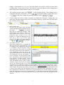
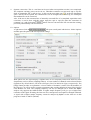
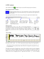
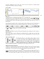
EPG systems, Wageningen, Netherlands
+
Stylet
versions:
User Manual
Free Software for EPG acquisition
and EPG analysis in Windows**-XP, -7 or -8
Software package parts
Shortcut icon to run EPG data acquisition (daq) for the Giga-8d
It also includes a routine for separate conversion; see Separate conversion.
Shortcut to run EPG signal analysis (ana) for Stylet+d acquired data files
Contents:
1.
2.
3.
4.
5.
Introduction
Installing and System requirements
Data Acquisition
EPG Analysis
Trouble shooting
1
1
2
4
10
* Latest versions always available on the downloads page of the website
** For Mac, see footnote page 2
Manual Stylet+ v01.25x.doc
January 2015
www.epgsystems.eu
1. Introduction
Stylet+ is Windows* based software package for EPG data acquisition and analysis of EPG signals. The
program is written in Delphy and replaces the earlier STYLET and PROBE software operating with
DOS and Windows 98, XP, respectively. Stylet+ can be used without any licence and is free
downloadable from www.epgsystems.eu. We are developing new versions regularly, the latest ones will
always be put on the website. We welcome any suggestions for improvements or additional features.
The Stylet+d data acquisition has been developed for Giga-8d hardware with build-in AD device for
analog-digital conversion and USB output signal for computer display and data file storage. Stylet+d
also replaces commercial EPG data acquisition software, as could be used for earlier Giga-4 and Giga-8
models.
The Stylet+a software has been especially developed for EPG analysis, using Stylet+d created data files.
Waveform analysis files are compatible with data processing software, such as Windows Excel macros
developed by the Julius Kuhn Institute (JKI, Quedlinburg, Germany) or by the Consejo Superior de
Investigaciones Científicas (CSIC, Madrid, Spain), or by the online EPG-Calc (INRA, Amiens, France;
http://www2.sophia.inra.fr/ID/SOFTS/epg/epg.php). The Stylet+a analysis part is very similar to the
earlier PROBE (Windows 98 - XP) and the old STYLET (DOS) analysis. Data files from both earlier
programs can be opened directly for analysis by Stylet+a.
Pictures from all Stylet+ screens can easily be saved and transferred to MS PowerPoint (or MS Word)
for use in publications or presentations.
2. Installing and system requirements
Installation
For installation, also see Stylet+ install.pdf file on the Downloads page of www.epgsystems.eu.
In fact the Giga-8d will be installed automatically when connected to the computer with internet
connection. The Giga-8d power should be switched on (display blue).
Note: there are two steps to be finished: finding and installing the driver for 1) the USB serial converter, and 2)
the COM port. Wait for a panel that confirms these installations has been finished, this may take a few minutes.
Minimum system requirements:
Windows* platform versions –me, -2000, -XP, -Vista, or -7
CPU ≥ 1GHz
RAM ≥ 512 MB
HD free space > 1GB
* Mac computers with bootable Windows environment will work as well and installation in the
Windows environment is identical. However, virtual Windows environment within the Mac
platform only works for Stylet+ analysis, not for data acquisition.
1
Windows settings: what NOT to do or TO DISABLE.
1. It is important to disable during data acquisition:
• Internet and network connections (no e-mail or updates should be possible!)
Disconnect internet and network of the computer.
• Screen saver ‘(none)’ if active
• Screen and HD switch down,
Set Power management options in Control panel to ‘never’
• Sleeping mode
2. Hide task bar: in START/Settings/Task bar and Start Menu, check [v] Auto-hide the taskbar.
3. DO NOT use other Windows activities whilst recording (data acquisition), no word processing or
other activities as these may interfere with or halt EPG recording.
3. Data Acquisition
Demo. If you are not used to EPG acquisition start without the USB cable connected.
After a double click on the
desktop icon the acquisition panel will be shown. In the bottom-R corner
you will see:
But it may be that in stead of Demo device you see:
/Undefined If so, move the mouse cursor to this text and the pop-up text: "Click to select recording device"
will appear. A click will then open the Select recording device panel. Click on "Demo device" and OK and a
4-channel acquisition in demo mode screen will appear containing the following sections:
1.
File naming: Give a name to the data file for your EPG signal file here. By default this file will be
stored in the C:\EPG_data folder but any other destination
can be selected by a click on the browsing icon
. The
program automatically will assign an .aq4 (or .aq8 for 8
channels) extension for this file, which is called the primary
acquisition file (see section below: file conversion and structure). Existing files with the extension
related to the USB device (.aq4 or .aq8) will be shown as well when browsing.
2.
Recording time: The box shows the in hours. Adjust this time to the time you want to record the
EPGs. Try to use complete hours, although not strictly
needed. The time is now 0.01h (about 37 sec) so mostly you
will need to adjust the recording time.
3.
Comments. Each file needs a header of 3 comment lines but only comments 2 and 3 can be edited.
Comment 1 will be adjusted automatically. The initial text
contains starting date and time, recording time and sampling
frequency after recording. Once ended, the text will be
changed in all real values. Comment 2 can be typed in the
box and it is wise to put here the treatments or experimental
conditions, plants, and insects used. Comment 3 can be used then to specify what channel will be
used for what treatment. Note that after acquisition separate files will be created for each channel so
that the treatment per channel (number) is crucial for the file contents.
4.
A mouse click on
initiates of the acquisition session and the
icon will appear,
which opens the opportunity to end this. The most direct visible effect is the EPG signal
becomes visible in the central white panel. At regular intervals a number of data points is
added to signal and when the signal reaches the right border it scrolls to the left making
space for new series of data points. Below the detailed one channel display a compressed
2
display of all channels (4 or 8) in a fixed time frame of 10 min is visible (at least if the
recoding time is longer than 10 min). The channel in the main display can be changed by a
mouse click on the channel button at the left, for example .
5.
The scrolling speed or time axis
of the detailed display of one channel can be
changed at two rates. A slow rate, showing
in the panel, and a six times faster rate,
of
in the panel. Change the speed by a mouse click on
or
.
6.
Several figures are shown during recording: recording time (duration), starting date and
clock time, the time elapsed since start of recording (progress), and the date and clock time
the recording will be ended.
7.
Inspect push button.
To freeze the top panel during recording
without interrupting the acquisition process
the inspect
button can be clicked.
This can be useful, for example, when
demonstrating some details to others. The
inspect panel can be resized or moved by
putting the cursor (mouse) to one of the
borders or a corner and dragging the size.
Also, the X and Y axis of the signal
as well as the range in the inspect panel, by
using
or
can be changed.
8.
File format converter.
When the recording time is finished, the
data is stored in one ‘intermediate file’ with
all samples of the recoding time from all 4
or 8 channels, with the extension .aq4 or
.aq8, respectively. These files are very big
and often contain unsuccessful channels as
well. Immediately after the end of the
acquisition session the file format converter
will change this big file into smaller, 1hour/1-insect files. To each of the new files
the 3 comment lines will be attached and to
each filename a channel number will be
added and also, the file extensions will be
.D## will indicate the hour, where ## here,
stands for a figure from 01-99. So, 99 hours
will be the maximum time for an EPG
acquisition session (although certainly not recommended!). During conversion the progress will be
visible by the green bar at the bottom and when ended the Conversion done message in the yellow
field is shown. Do not take any actions as long as this message is not shown! The converted files will
be stored in the folder as the file destination (directory) as indicated in the ‘intermediate file’ space.
This information is followed by another line giving the Sample rate and the number of channels
used. The sample rate is also given in comment line 1, i.e. the sample rate that has been really made
during the acquisition session and should not deviate more than 5% from 100 Hz defined by the
software.
3
9.
Separate conversion. This is a tool that can be used when an acquisition session is not completed.
The computer can hang; power can be cut, etc. Then there remains a not converted .aq4 or .aq8 file.
Such an incomplete file is still not lost. A click on the most right icon
in the file destination
space. The file can be opened, the comment lines can be changed and successively, the incomplete
intermediate file can be converted.
Also, if the text in the comment lines of normally converted files of a completed acquisition needs
correction, it can be done with this option. Open the .aq4 or .aq8 file, make the corrections in
comment 2 or 3 and click on the
button. The new converted file will overwrite the existing,
previously automatically converted files.
10. Options
A right mouse click on
will open a small panel with choices. Select 'Options'
and this opens the panel with data acquisition settings.
With update rate, the signal display is updated more or less frequently which looks better but more
frequent may cause overruns (sampling failures). A lower number of channels can be selected for the
Giga8d (or any old AD device; Di710 for old Giga-8, Di155 or Di158 for Giga-4, respectively). The
[Help] button provides an explanation. A lower number of channels is useful if not all channels (of
the Giga-4 or -8) will be used in a certain experiment, thus avoiding deletion of empty files from not
used channels are used. The sampling frequency can also be changed but be aware that Stylet+
analysis only supports the 100Hz default. A higher sample frequency will give you a higher time
resolution of the signal. Warning: the later two have consequences and cannot be changed unlimited.
A signal with a higher sample frequency cannot be analysed by Stylet+a as the time axis in this
program is based on 100 Hz (default).
4
4. EPG Analysis
After a double click on
the Stylet+ analysis icon the EPG analysis panel will shown.
File loading and header comments
Pushing this button will get you a file selection box to open any first hour data file
(--.D01). Select the file you want and click open. The first hour of the signal will be
shown shortly.
The following information will be shown on top of the panel, right from the START button.
data file
location.
and file
name
comment 1 recording
start clock time, date,
recording time, and
sample frequency made
experimental conditions channel
plant cv., aphid + stage
specific
leaf exposed for EPG
information
present hour
and access to
prev./next
hour
Moving around
The displayed hour is hour 1, file -.D01, see file location information.
Pressing the [H >] button will load the next hour, if available. If there is
no next hour a ‘file does not exist’ information box will be displayed.
Similarly the previous hour will be opened when clicking the [< H]
button.
1 HOUR display
The complete one hour (3600 sec) display shows a time axis in seconds from start of the first
hour (time 0). The Y scale, −5 to +5 Volts, represents the output voltage of the Giga-amplifier.
NOTE: The input voltage (at input of the first stage amplifier [EPG Probe]) might be inferred from the –50
mV calibration pulse, when pushing the CAL. button (red button on the Giga device) during EPG recording.
See, Giga4/8 manual.
The slider bar below the 1H graph shows a green slider, initially at the left end, the beginning
of the hour. Its width corresponds with the number of seconds of the frame size, which is
shown in the lower DETAIL panel (the yellow area in the graph also reflects this frame, but
widening this area by dragging the left or right black line border
has no meaning
5
presently). Dragging the green slider and a click on any new slider bar or signal position
changes the detail frame position accordingly.
DETAIL
panel
Frame size
As displayed here, by default the detail frame size is 30 seconds. By
clicking the down or up arrowhead the frame size can be decreased
or increased, respectively. Values of 5, 10, 30, 60, or 100 seconds can be selected, allowing you
to change the time frame of the detail and the green slider square and yellow area in the 1 h
display panel.
The starting time position of the 1 h (green) slider and the starting time in the detail frame is
displayed in seconds between the 1h and detail display panel, at the centre in green (0 here).
Left and right from this, two frame shift buttons will move the detail frame by a discrete step of
0.5
or 0.1 of the frame size, to the left or to the right.
Scrolling
Keeping the ENTER key pressed will keep the shift going, thus scrolling to the left or right at a
different speed.
Other scroll effects can be achieved by pressing the left or right arrow key but some
uncontrolled changes will occur. The frame size will be changed and the scroll step will mostly
be 0.1 frame.
Offset and voltage scale
By default the offset is 0 volts and the Output voltage (Y-scale)
is ±5 Volts. The offset can be changed by dragging (L mouse
key kept pressed) or after a click on the slider you can use the up
and down arrow keys. The voltage scale is only changed by
dragging the slider to any of the ther ranges. As this often will
lead to a signal position near or outside the edge of the graph
frame the adjustments should be coordinated to keep the signal in the frame area.
Signal feature observation tools
In addition to displaying different hours and details in different X (time) and Y (output voltage)
resolution two other observation tools can enable the analysis of waveform features, Smooth
and Spectrum. To access these tools click on
and then on the name of the tool.
Smooth will selectively filter out 50-60 Hz noise, if this may mask some signal details (Note: as
indicated in the Giga-4/8 manual, preventing noise is much better than removing the noise by
smooth). The filtered signal will appear in the detail frame only in red. As soon as the frame
6
position is changed the original (noisy) signal will reappear so that each new detail requires
another smooth action, if needed. In the smoothened signal the cursor operations remain
unchanged.
Filter
Similar to Smooth but now at every frequency wanted a low pass, high pass, or band pass
filtering of the Detail panel signal can be executed. Type the frequency value(s) in the picture.
Spectrum will give a new display panel in a
separate window with the auto power
spectrum graph, i.e. a frequency analysis of
the first 10 seconds of the signoal after the
beginning of the detail graph signal (if the
frame is 10s or longer). The auto power
spectrum graph comes from the fast Fourier
transform and gives the frequency in Hz (Xaxis) and the magnitude (Y-axis), i.e. the
contribution of the frequencies occurring in
this 10s of the signal. The spectrum may help
in estimating the EPG waveform.
NOTE: Frequency analysis is only useful when a sine wave like signal or regular repetition of
signal elements occurs. Irregular signals will not provide a clear APS.
Cursor in detail display panel
A mouse click within the graph will cause a red cursor line to appear. Its time position is in
seconds and the output voltage in mV is displayed in red below the detail display panel.
Cursor movement
A new mouse click in a different location within the detail display will cause a new cursor
position, which also can be moved forward in two different ways. When the
mouse arrow is close to the red cursor line the ◄││► mark will be shown and by
keeping the left mouse key pressed the cursor can be dragged to any position in
the detail display panel. Also very small movements of only one data point (100 points/sec) to
the left or right can be made by a mouse click on the left or right position button.
Retrieving data from the EPG signals
So far the analysis properties were about moving around, getting details, displaying frequency
features, removing noise by smoothening and putting the cursor at any possible position (time).
From this information we can derive or recognise biologically relevant ‘waveforms’. This is not
automatically done by Stylet+. You will need to learn waveform recognition. In the appendix a
list of aphid waveforms and correlations is provided. The layout Stylet+ has been based on
aphid EPGs but can be used very well for any other group of piercing-sucking insects; see the
section ‘Other insects’ (p. 12)
After waveform recognition, we want to get from EPGs when waveforms start how long they
last and in what sequence. This is what the Stylet+ analysis software is made for. It is the crucial
analysis activity that precedes further data processing.
7
Stylet+ data retrieving
In Stylet+ waveform labels are assigned to the readout buttons below the detail display panel.
Pressing a waveform button reads the coordinates (time and voltage) at the red cursor line
position and stores its values in the Analysis grid with the value of the waveform specific
button. The cursor should be moved to the start of each successive waveform and the respective
button pressed. So, going through the signal from the beginning to the end of the last hour
visual recognition and cursor-button activity will cause a many lines in the analysis grid, one
line for each waveform change. The assumption is that waveforms – the insect’s probing
activities – are mutually exclusive, i.e. waveforms are not occurring simultaneously and the
start of a new one implies that the previous waveform stops. Although not strictly true, this
assumption is very suitable. The main exception in aphids is made by waveforms A, B, and C,
together representing ‘stylet pathway phase’ of probing. We ‘solved’ this overlap problem by
lumping these waveforms as ‘waveform C’ which as such now is the mutually exclusive with
the other waveforms.
Readout buttons/function keys
Readout buttons are numbered in accordance to the Keyboard function keys, which are
equivalent to pushbuttons. For aphids button 9 and 10 will appear only when the pd button (8)
has been pressed and disappear after pushing the C button (2). This is to emphasise that the
analysis of the pd waveforms and its (mostly difficult to distinguish) sub-phase transients is
optional. Although the pushbuttons 9 and 10 only appear when button/function key 8 has been
used, function keys 9 and 10 will work at any time.
Thus for other insects, neglect the aphid waveforms and use the function key numbers coding
for the other insect’s waveforms.
Defined waveform labels: non-aphid waveforms
The aphid waveforms buttons are the default settings of Stylet+ analysis. For other insects you
can create other button labels. To assign other labels to the buttons select the option ‘Define
waveform labels’ in the
. A Define Wave Labels panel will open. Remove the checkbox v
by a mouse click, and type the new labels in the buttons, then click on [save as] and give the
new set of button labels a name. Finally click on Apply “new name” and you will see the
button names implemented. After closing Stylet+ analysis in the next opening the last used
button set will be shown. Changing then to aphid waveform buttons is done by clicking the
checkbox, showing the v again and with a mouse click on [Apply “Default”] aphid mode is
restored. Correction in any new set can be made in the same Define Wave Labels panel
followed by [ save ]. Several sets of buttons can be made and one can switch from one set to
the other in the drop down list below the “Select user defined wave names”
Note: the first 3 characters of the button set name will be added to the file name of the saved
grid when using the changed wave button mode.
8
Table of buttons and aphid waveforms
Button code/F-key
aphid waveform
[np]
[C]
[E1e]
[E1]
[E2]
[F]
[G]
[pd]
[II-2]
[II-3]
[11]
[12]
[T]
non penetration
stylet pathway phase, including waveforms A, B, C, and pd
E1 extracellular (not always shown)
E1, normal phloem salivation
E2, phloem feeding
F, stylet penetration difficulties
G, xylem drinking
pd, in addition to [C] for separate pd analysis (not recommended)
sub-phase II-2 of a pd (if analysed)
sub-phase II-2 of a pd (if analysed)
extra button/code for any use (activity event or as a marker)
extra button, as [11]
terminus, total recording time (s) as derived from all hours available in
data files. The number 99 can be used in further data processing
routines.
1
2
3
4
5
6
7
8
9
10
11
12
99
Analysis grid
Pressing a waveform button (or function key) stores the numerical waveform code, and the
cursor coordinates (s and mV) in the Analysis grid in a row with 3 columns, Wave, Start, and
mV, respectively. Each new button/function key push inserts a new row but only the last 4
readout lines are visible. Earlier rows need use of the vertical scroll bar right of the grid.
Automatically each new row is inserted in accordance to the start time, highest value on top.
Grid corrections
Wrong readouts or mistakes can be corrected by selecting the cell (turns light blue) and typing
the correct value and an Enter key stroke or selecting another cell. A complete line can be
removed by selecting a cell in the row, then press
and select ‘Delete row’.
Double readout warning
If by mistake the same waveform button has been pushed
again, resulting in two successive rows with same wave
code a warning appears. Meanwhile, the grid will change to
red until a correction is made. Note this warning will also
occur when a row is deleted between two rows with same
wave code. Pushing a key with a different wave code and a
start time between the two rows will then result in a correct
sequence and the warning will disappear.
Grid value to cursor position.
Upon a mouse a click on a grid wave cell will highlight the cell and jump the cursor to the
corresponding position in the signal and vice versa, a click on the signal will move to and
highlight the corresponding grid cell as long as the frame contains the position.
9
End of analysis
When all waveform changes have been put in the grid, press the
button to add the complete
recording time, which is the (artificial) end of the last waveform as well. This value will be
used by the data processing macros and on line routines (see www.epgsystems.eu page data
processing.
Save grid
When the analysis of a recording is finished the information should be saved. Select the ‘Save
this grid’ option in the
and the grid data will be save in a .ana file, to which a file name
will be assigned/suggested automatically that is derived from the data filename. Accept or
change this name and the location where it will be saved.
Interrupting and Resuming an Analysis
You one can interrupt EPG analysis at any time and resume it later. To do so, load the .D01 file
again (click on .START. and select the file), then in the
select ‘Load other grid’ and select
the interrupted .ana file, which will loaded in the grid allowing resuming the analysis on the
point of the previous interruption. Also any analysis key strokes can be added to/inserted into
the existing analysis grid.
Next analysis in the same Stylet+ session
When loading another file the grid contents will not
automatically be deleted for safety reasons. An information
panel will pop up to remind you. The grid should be cleared
manually by selecting the ‘Clear grid’ option in the
.
All
options
All options are briefly explained in the ‘Help’ option.
Tool, in display panels
Both signal display panels, the 1h and the Detail panel have this magnifying glass tool in the
bottom left corner. A click on this button will show a separate display panel with the same
signal as the display panel (similar to the [inspect] button in the Stylet+ acquisition program),
which allow
zooming in and out and auto scaling, respectively. And also, shifting
up/down
(Y axis, voltage) and left/right
(X axis, time). Such a separate panel is shown
also for the Spectrum option in the
.
The source file and the start and ending time are shown in the blue label on top of the signal.
As you can see in the example the source file name is followed the 10s time frame, in the
example here (page 5):
Copy and paste of display panels
Display panels after using the
can be copied by a mouse click on the
icon and pasted into
Windows documents, spreadsheets, or presentations.
Note: Pasting by the ‘paste’ command (after a right mouse click) or Ctrl V will paste the figure
but editing the figure after ‘ungrouping’ will not be possible then. To keep the ungrouping and
successive possibilities open, it is necessary to paste the figure by selecting ‘Paste special’
command in the View dropdown list and then select emf. Only pasted by this method allows
editing, which can be done best in Windows PowerPoint (better than in Word!).
The picture can also be saved as .bmp by clicking the
10
icon.
Trouble shooting & error messages
File size
The converted one insect/one hour files will normally contain 360.000 data points each.
However, the last hour may contain somewhat less points or there will appear an extra hour
with only a few data points, depending on small deviation between the real sample frequency
and exact 100 Hz sample frequency. No serious on the analysis results will be caused by
differences up to 10-20 seconds in a recording time of several hours.
Overruns
During acquisition on the bottom bar the number overruns is displayed. This number should be
as low as possible. The number increases if other programs are on or used during recording or
the computer is connected to intranet or internet. Disable these connections during data
acquisition and don’t use other programs on the computer during EPG recording!
Error 103
At [Start] of the analysis routine, Stylet+a this error message will be shown when the data file
(.D01) is a ‘read only’ file. The read only property may sometimes be initiated during file
transfer or copying. If put on CDRom files will always be changed to read only files. In
explorer a R mouse click and subsequent selection of Properties allows you to remove the read
only check property and make the file accessible but on a CDRom this cannot be changed and
files should be copied first to your hard disk for use in Stylet+a.
11