Download GLuskap 2.4 - University of Lethbridge

GLuskap 2.4
User’s Manual
GLuskap
User’s Manual
Three-Dimensional Graph Drawing Software
Breanne Dyck,
Sebastian Hanlon,
Stephen Wismath
University of Lethbridge,
Lethbridge, Alberta, Canada
Funded in part by:
Natural Sciences and Engineering Research Council of Canada
c
Copyright °2004
Stephen Wismath. All rights reserved.
This document does not convey a warranty, express or implied, of merchantability or fitness for a particular purpose.
GLuskap Version 2.4
Manual made with LATEX
Credits:
• GLuskap version 2.x was written by Breanne Dyck, Sebastian Hanlon
and Jill Joevenazzo under the supervision of Dr. Stephen Wismath at
the University of Lethbridge in 2004.
• GLuskap version 1.x was written by Breanne Dyck, Jill Joevenazzo,
Elspeth Nickle, and Jon Wilsdon.
License:
• GLuskap is freely available and distributed under the terms of the GNU
General Public Licence.
Acknowledgments:
• Zac Friggstad, Kim Hansen, Jill Joevenazzo, and Elspeth Nickle contributed to the testing of this software.
• A GLuskap (MG2) import plugin for 3D Studio Max was written by
Kim Hansen.
iv
Contents
1 Introduction
1.1 Obtaining GLuskap . . . . . . . . . . .
1.1.1 System requirements . . . . . .
1.1.2 Win32/x86 stand-alone . . . . .
1.1.3 Python source . . . . . . . . . .
1.2 Installing GLuskap . . . . . . . . . . . .
1.2.1 Win32/x86 stand-alone installer
1.2.2 Win32/x86 stand-alone zip . . .
1.2.3 Source packages . . . . . . . . .
1.3 Terms and Conventions . . . . . . . . .
1.3.1 Representation of Graphs . . .
1.3.2 Restrictions on Graphs . . . . .
1.3.3 File Format . . . . . . . . . . .
1.3.4 Visual Conventions . . . . . . .
1.4 Feedback . . . . . . . . . . . . . . . . .
.
.
.
.
.
.
.
.
.
.
.
.
.
.
.
.
.
.
.
.
.
.
.
.
.
.
.
.
.
.
.
.
.
.
.
.
.
.
.
.
.
.
.
.
.
.
.
.
.
.
.
.
.
.
.
.
.
.
.
.
.
.
.
.
.
.
.
.
.
.
.
.
.
.
.
.
.
.
.
.
.
.
.
.
.
.
.
.
.
.
.
.
.
.
.
.
.
.
.
.
.
.
.
.
.
.
.
.
.
.
.
.
1
1
2
2
2
3
3
3
3
3
3
4
4
5
5
2 Using GLuskap
2.1 Interface Layout . . . . . . . . . . . . . . . . . . .
2.1.1 Interface Overview . . . . . . . . . . . . .
2.2 Creating Graph Elements with the Panel . . . . .
2.2.1 Creating Vertices . . . . . . . . . . . . . .
2.2.2 Creating Edges . . . . . . . . . . . . . . .
2.3 Editing Graph Elements with the Panel . . . . . .
2.3.1 Selecting Graph Elements . . . . . . . . .
2.3.2 Editing Vertices . . . . . . . . . . . . . . .
2.3.3 Deleting Vertices . . . . . . . . . . . . . .
2.3.4 Editing Edges . . . . . . . . . . . . . . . .
2.3.5 Bending Edges . . . . . . . . . . . . . . .
2.3.6 Deleting Edges . . . . . . . . . . . . . . .
2.4 Using the Graph Display Panel . . . . . . . . . .
2.4.1 Ground Plane and Axes . . . . . . . . . .
2.4.2 Heads-Up Display . . . . . . . . . . . . . .
2.4.3 Navigating with the Keyboard and Mouse
2.4.4 Orthogonal View . . . . . . . . . . . . . .
2.4.5 Vertex Axes . . . . . . . . . . . . . . . . .
.
.
.
.
.
.
.
.
.
.
.
.
.
.
.
.
.
.
.
.
.
.
.
.
.
.
.
.
.
.
.
.
.
.
.
.
.
.
.
.
.
.
.
.
.
.
.
.
.
.
.
.
.
.
.
.
.
.
.
.
.
.
.
.
.
.
.
.
.
.
.
.
.
.
.
.
.
.
.
.
.
.
.
.
.
.
.
.
.
.
.
.
.
.
.
.
.
.
.
.
.
.
.
.
.
.
.
.
.
.
.
.
.
.
.
.
.
.
.
.
.
.
.
.
.
.
7
7
8
8
8
10
10
10
11
11
11
11
12
12
12
13
13
14
14
.
.
.
.
.
.
.
.
.
.
.
.
.
.
.
.
.
.
.
.
.
.
.
.
.
.
.
.
.
.
.
.
.
.
.
.
.
.
.
.
.
.
.
.
.
.
.
.
.
.
.
.
.
.
.
.
.
.
.
.
.
.
.
.
.
.
.
.
.
.
v
CONTENTS
2.5
GLuskap Menus . .
2.5.1 File Menu .
2.5.2 Edit Menu .
2.5.3 View Menu
2.5.4 Tools Menu
2.5.5 Help Menu .
.
.
.
.
.
.
.
.
.
.
.
.
.
.
.
.
.
.
.
.
.
.
.
.
.
.
.
.
.
.
.
.
.
.
.
.
.
.
.
.
.
.
.
.
.
.
.
.
.
.
.
.
.
.
.
.
.
.
.
.
.
.
.
.
.
.
.
.
.
.
.
.
.
.
.
.
.
.
.
.
.
.
.
.
.
.
.
.
.
.
.
.
.
.
.
.
.
.
.
.
.
.
.
.
.
.
.
.
.
.
.
.
.
.
.
.
.
.
.
.
.
.
.
.
.
.
.
.
.
.
.
.
.
.
.
.
.
.
.
.
.
.
.
.
14
14
17
17
19
21
A MG2 Technical Reference
A.1 Overview . . . . . . . . . . . .
A.1.1 Formal Representation
A.1.2 Examples . . . . . . .
A.1.3 Further examples . . .
A.2 Record Description Format . .
A.3 Record Formats . . . . . . . .
A.3.1 fileformat . . . . . . .
A.3.2 vert . . . . . . . . . .
A.3.3 dummy . . . . . . . .
A.3.4 edge . . . . . . . . . .
A.3.5 super . . . . . . . . . .
.
.
.
.
.
.
.
.
.
.
.
.
.
.
.
.
.
.
.
.
.
.
.
.
.
.
.
.
.
.
.
.
.
.
.
.
.
.
.
.
.
.
.
.
.
.
.
.
.
.
.
.
.
.
.
.
.
.
.
.
.
.
.
.
.
.
.
.
.
.
.
.
.
.
.
.
.
.
.
.
.
.
.
.
.
.
.
.
.
.
.
.
.
.
.
.
.
.
.
.
.
.
.
.
.
.
.
.
.
.
.
.
.
.
.
.
.
.
.
.
.
.
.
.
.
.
.
.
.
.
.
.
.
.
.
.
.
.
.
.
.
.
.
.
.
.
.
.
.
.
.
.
.
.
.
.
.
.
.
.
.
.
.
.
.
.
.
.
.
.
.
.
.
.
.
.
.
.
.
.
.
.
.
.
.
.
.
.
.
.
.
.
.
.
.
.
.
.
23
23
23
24
24
25
25
25
25
26
26
26
B Included Sample Graphs
27
B.1 Samples in MG2 Format . . . . . . . . . . . . . . . . . . . . . 27
B.2 Samples in External Formats . . . . . . . . . . . . . . . . . . . 27
vi
List of Figures
2.1
2.2
2.3
2.4
2.5
2.6
2.7
2.8
2.9
2.10
2.11
2.12
2.13
2.14
The basic user interface (Linux/GTK)
Graph Display panel . . . . . . . . . .
Graph selection tabs . . . . . . . . . .
Vertex and edge properties . . . . . . .
Vertex and edge lists . . . . . . . . . .
Graph Display camera controls . . . .
The world axes . . . . . . . . . . . . .
Heads-Up Display . . . . . . . . . . . .
Vertex Axes . . . . . . . . . . . . . . .
POV-Ray Export Options . . . . . . .
Circle Layout Example . . . . . . . . .
Butterfly Layout Example . . . . . . .
Random Layout Example . . . . . . .
Spring Layout Example . . . . . . . . .
.
.
.
.
.
.
.
.
.
.
.
.
.
.
.
.
.
.
.
.
.
.
.
.
.
.
.
.
.
.
.
.
.
.
.
.
.
.
.
.
.
.
.
.
.
.
.
.
.
.
.
.
.
.
.
.
.
.
.
.
.
.
.
.
.
.
.
.
.
.
.
.
.
.
.
.
.
.
.
.
.
.
.
.
.
.
.
.
.
.
.
.
.
.
.
.
.
.
.
.
.
.
.
.
.
.
.
.
.
.
.
.
.
.
.
.
.
.
.
.
.
.
.
.
.
.
.
.
.
.
.
.
.
.
.
.
.
.
.
.
.
.
.
.
.
.
.
.
.
.
.
.
.
.
.
.
.
.
.
.
.
.
.
.
.
.
.
.
.
.
.
.
.
.
.
.
.
.
.
.
.
.
7
8
8
9
9
9
12
13
15
16
19
20
20
21
vii
LIST OF FIGURES
viii
Chapter 1
Introduction
GLuskap1 is a tool for creating, modifying, and displaying graph drawings
in three dimensions. Support is provided for drawing graphs with straight
lines, bent edges, orthogonally, etc. Graphs can be labelled and coloured
and the resulting drawing can be output in a variety of formats. Navigating,
editing, and modifying the layout of the graph drawing is of particular utility
to the graph drawing community, as to date there are very few packages for
graph manipulations in three dimensions. See for examples Graph Drawing
Software, Jünger and Mutzel 2004. Our main focus has not been to provide
a broad range of layout tools (we provide only some simple standard layouts
such as a 3D spring embedder) but rather to focus on interactive graph
manipulation and the export of the drawings as high-quality images.
The initial version of GLuskap was written in C++ using the SDL library
and was presented as a poster at the Graph Drawing 2003 conference. The
current version (2.x) is a complete re-write of the software and is written
in Python using OpenGL. Support for stereo viewing using stereoglasses is
provided.
GLuskap is part of a suite of tools developed at the University of Lethbridge for computational geometry and graph drawing in two and three dimensions, available from:
http://www.cs.uleth.ca/~wismath/packages/.
1.1
Obtaining GLuskap
Several distributions of GLuskap are available, depending on computing platform and the resources available in the working environment. The most
recent GLuskap packages are available from:
http://www.cs.uleth.ca/~wismath/packages
1
The name “GLuskap” is derived from the Algonquin term for the “creator force”.
Introduction
1.1.1
System requirements
GLuskap is developed on GNU/Linux and Microsoft Windows 2000 and has
been tested on Mandrake Linux, Debian GNU/Linux, Windows 98, Windows
XP, and OSX Panther. As GLuskap is written in Python, it may run on your
favourite platform even if it is not listed here; try the source package.
On all platforms, GLuskap requires a graphical window environment (X/Motif,
X/GTK, Apple OSX/Carbon, Microsoft Windows) with OpenGL support.
A video device supporting OpenGL accelleration is highly recommended for
performance reasons. While not strictly required, a mouse is also strongly
recommended for navigation.
Stereographics support requires a video device supporting OpenGL quadbuffering.
1.1.2
Win32/x86 stand-alone
This distribution includes all the Python runtimes and supporting libraries
and is suitable for most users who do not want to install a complete Python
environment with all the dependancies. As a result, the package and the
installed disk space footprint are both larger than the other distributions.
Two packages are available:
• gluskapX Y Z-install.exe is a self-extracting installer package that
will create shortcuts and includes a friendly uninstaller. May require
administrative privileges to install.
• gluskapX Y Z-win32.zip is a zip archive that can be unpacked and
run from any location. Does not require administrative privileges.
1.1.3
Python source
The GLuskap Python source distribution requires a Python 2.3 runtime environment, along with these supporting packages:
• wxPython version 2.5.2.7 or later
<http://www.wxpython.org/download.php>
• PyOpenGL version 2.0.1.07 or later
<http://pyopengl.sourceforge.net>
• numarray version 1.0 or later
<http://www.stsci.edu/resources/software hardware/numarray>
• GLUT/GLE version 3.6 or later
<http://www.opengl.org/resources/libraries/glut/glut downloads.html>
2
1.2. Installing GLuskap
As Python and OpenGL are portable packages, these dependancies should
be available on most popular platforms.
Two source packages of GLuskap are available, although their contents are
identical.
• gluskapX Y Z-source.tar.gz is intended for Unix-like platforms.
• gluskapX Y Z-source.zip is intended for Microsoft Windows platforms.
GLuskap is freely available under the terms of the GNU General Public
Licence. It is included in all packages as the file LICENSE.
1.2
1.2.1
Installing GLuskap
Win32/x86 stand-alone installer
If using the installer package, download and run the installer. It will prompt
for the location to install GLuskap and whether you want to create Start
Menu shortcuts. Run GLuskap using the shortcuts.
1.2.2
Win32/x86 stand-alone zip
Uncompress the zip package in the desired location. The GLuskap distribution is contained in the directory GLuskap-X-Y-Z. To use GLuskap, run
gluskap.exe.
1.2.3
Source packages
Uncompress the source package in the desired location. To use GLuskap,
run gluskap.py with your installed Python interpreter. If dependancies are
missing or outdated, you may encounter errors. Note that under Mac OS
X, GLuskap should be run from the command line, rather than through the
Python IDE—due to threading problems with the IDE, it may cause GLuskap
to crash.
1.3
Terms and Conventions
1.3.1
Representation of Graphs
A graph in GLuskap is represented by a list of vertices and a list of edges.
Each edge has one and only one source vertex and one and only one target
vertex.
Vertices are identified by a vertex ID, which can be any string value.
Vertex IDs must be unique within a given graph.
3
Introduction
Edges are identified by a unique pair of distinct vertices. Each edge must
be unique within a given graph.
1.3.2
Restrictions on Graphs
GLuskap supports only undirected edges; the labels “source” and “target”
are used for convenience only.
An edge (a, a) with identical source and target is called a degenerate
edge and is disallowed within GLuskap.
Any pair of edges {(a, b), (a, b)} or {(a, b), (b, a)} are considered duplicate
edges and are disallowed. GLuskap allows only one edge between any pair of
vertices.
Note that GLuskap does not check for intersections between pairs of edges
in 3D; if required, such detection is the responsibility of the user.
1.3.2.1
Bent Edges
Edges described by polylines (a.k.a. “bent edges”) are supported by GLuskap.
A bent edge is represented in GLuskap by a superedge: an ordered set of
dummy vertices representing bend points and subedges connecting these
vertices in order.
Dummy vertices must be of degree 2 and must be associated with a bent
edge. Deleting a dummy vertex in a bent edge with at least two bends will
cause the bent edge to snap between the adjacent dummy vertices. Deleting
the last dummy vertex in a bent edge will un-bend the edge. The bent edge
to which a dummy vertex belongs is called its parent.
A vertex in the graph that is not a dummy vertex is called a proper
vertex for convenience in ambiguous contexts.
Subedges, i.e. edges between a proper vertex and a dummy vertex or
between two dummy vertices, will appear in the edge list of the graph in
addition to the superedge to which they belong.
1.3.3
File Format
The default format used by GLuskap 2.4.x to store graph drawings is called
MG2 , and is described in Appendix A: MG2 Technical Reference. For legacy
reasons, GLuskap also supports the deprecated GLuskap 1.x MG file format,
although its use is discouraged. Note that not all features are available in
the MG format.
GLuskap also supports importing and exporting from GraphML and
GML, for compatibility with other popular graph drawing and graph manipulation products.
4
1.4. Feedback
1.3.4
Visual Conventions
GLuskap uses a right-handed coordinate system to describe the perpendicular orientation of each axis with respect to the remaining two. By convention, positive Y is the “up” direction, and if the viewer is looking at the
origin with the positive X on their “right”, positive Z is towards the viewer.
Where coloring is used in the interface to indicate axes, red is used for X,
green is used for Y, and blue is used for Z.
1.4
Feedback
The GLuskap team welcomes your comments, bug reports, and suggestions
for the future development of GLuskap. The latest version, bug tracking
services, and contact information are all available from the GLuskap web site:
http://www.cs.uleth.ca/~wismath/packages/.
5
Introduction
6
Chapter 2
Using GLuskap
Running GLuskap without any arguments, or from a shortcut, will start
GLuskap with an empty graph loaded.
2.1
Interface Layout
The basic user interface is shown in Figure 2.1. Note that the appearance of
the interface may vary slightly depending on your operating environment, as
GLuskap uses the wxPython cross-platform toolkit to create a GUI consistent
with the user’s environment. GLuskap’s functionality is the same regardless
of the operating environment.
Figure 2.1: The basic user interface (Linux/GTK)
7
Using GLuskap
2.1.1
Interface Overview
The GLuskap interface has several parts.
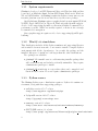
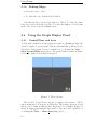
Figure 2.2: Graph Display panel
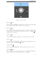
Figure 2.2 shows the graph display panel. When a graph is created or
loaded, it will be displayed here. Clicking on the panel allows you to change
the camera position and orientation. See: Using the Graph Display Panel
Figure 2.3: Graph selection tabs
Figure 2.3 shows the graph selection tab bar. GLuskap allows multiple
graphs to be loaded concurrently. The tab bar allows the user to switch
between open graphs.
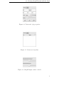
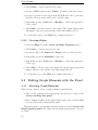
Figure 2.4 shows the vertex and edge properties panel, used for creating
and editing vertices and edges. Figure 2.5 shows the vertex and edge lists,
including subedges, and can be used to select graph elements.
See 2.3: Editing Graph Elements with the Panel
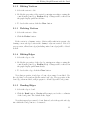
Figure 2.6 shows the display panel camera controls. These controls affect
the movement of the camera when navigating inside the graph drawing. See
2.4: Using the Graph Display Panel
2.2
2.2.1
Creating Graph Elements with the Panel
Creating Vertices
1. Select the Vertex tab in the Vertex and Edge Properties panel.
8
2.2. Creating Graph Elements with the Panel
Figure 2.4: Vertex and edge properties
Figure 2.5: Vertex and edge lists
Figure 2.6: Graph Display camera controls
9
Using GLuskap
2. Click Clear to deselect any selected vertex.
3. Specify an ID (required) and a Name (optional) for the new vertex.
4. Specify a position for the vertex in the X/Y/Z fields. If no position is
specified, the new vertex will be placed at the origin.
5. Optionally, specify a Color and/or Radius to control the appearance
of the vertex.
6. Click Add to add the vertex to the graph. The graph display panel
will jump to the new vertex and the vertex will remain selected.
To add another vertex, click Clear and continue with step 3.
2.2.2
Creating Edges
1. Select the Edge tab in the Vertex and Edge Properties panel.
2. Click Clear to deselect any selected edge.
3. Specify the IDs of the Source and Target vertices of the new edge.
4. Optionally, specify an Attribute for the edge.
5. Optionally, specify a Color and/or Radius to control the appearance
of the edge.
6. Click Add to add the edge to the graph. The graph display panel will
jump to the new edge and the edge will remain selected.
To add another edge, click Clear and continue with step 3.
2.3
2.3.1
Editing Graph Elements with the Panel
Selecting Graph Elements
There are two ways to select a graph element for modification:
1. Click on the element in the appropriate list (vertex or edge) in the
Vertex and Edge List panel.
2. If the element is visible in the graph display panel, hold down the Ctrl
key and click on the element in the panel.
This will switch to and populate the appropriate tab in the Vertex and
Edge Properties panel. Note that only one graph element may be selected
at a time.
10
2.3. Editing Graph Elements with the Panel
2.3.2
Editing Vertices
1. Select the vertex to edit.
2. Modify the properties of the vertex by entering new values or using the
controls in the panel (e.g. Radius slider). Changes will be reflected in
the graph display panel in real time.
3. To deselect the vertex, click the Clear button.
2.3.3
Deleting Vertices
1. Select the vertex to delete.
2. Click the Delete button.
If the vertex is a dummy vertex, deletion will result in its parent edge
forming a new subedge between the dummy’s adjacent vertices. If it is a
proper vertex, all incident edges (including entire bent edges) will be deleted
as well.
2.3.4
Editing Edges
1. Select the edge to edit.
2. Modify the properties of the edge by entering new values or using the
controls in the panel (e.g. Radius slider). Changes will be reflected in
the graph display panel immediately.
3. To deselect the edge, click the Clear button.
Note that properties of subedges of bent edges cannot be modified. Use
the edge list to select and modify the entire bent edge. The properties of the
bent edge, when modified, will propagate to all subedges and bend points.
2.3.5
Bending Edges
1. Select the edge to bend.
2. Click the Bend button. GLuskap will prompt you for the coordinates
of the bend point. The default is the origin.
Note that superedges cannot be bent. Instead, select the specific subedge
into which the bend point is to be inserted.
11
Using GLuskap
2.3.6
Deleting Edges
1. Select the edge to delete.
2. To delete the edge, click the Delete button.
Note that subedges of bent edges cannot be deleted. To delete the entire
bent edge, select it from the edge list. To reduce the number of bend points
in the edge, delete a specific dummy vertex.
2.4
2.4.1
Using the Graph Display Panel
Ground Plane and Axes
To help with orientation in the graph view window, GLuskap provides the
option to display a “ground plane” which is automatically positioned below
all vertices of the graph. It can be switched on or off using the View —
Show Ground Plane menu option. The ground plane is visible in Figure
2.2; it’s the darker bottom half of the panel.
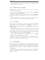
Figure 2.7: The world axes
The world X, Y, and Z axes can also be displayed for reference. The X
axis is drawn in red, Y in green, and Z in blue. The positive direction of each
axis is colored darker and the negative direction is colored lighter. Figure 2.7
shows an empty graph with the axes enabled. The axes can be switched on
or off using the View — Show Axes menu option.
12
2.4. Using the Graph Display Panel
Figure 2.8: Heads-Up Display
2.4.2
Heads-Up Display
Figure 2.8 shows the navigation heads-up display (HUD).
The upper part shows the camera orientation relative to the world. A
top-down view shows bearing in the X-Z plane The side view shows elevation
from the X-Z plane. On both, the yellow cone approximates the camera’s
field of view, and the red marker points toward the origin.
The lower part shows the X, Y, Z coordinates of the camera location, in
red, green and blue respectively.
The HUD can be switched on or off using the View — Show HUD
menu option.
2.4.3
Navigating with the Keyboard and Mouse
Clicking and dragging with the mouse on the graph display panel will pan and
tilt the camera view. The camera position can be moved with the keyboard.
The speed of camera movement and rotation can be controlled using the
sliders on the Graph Display camera control panel, shown in Figure 2.6.
If there is a vertex selected, the keyboard can be used to move it in unit
increments.
Table 2.1 shows the keyboard commands available. Before using keyboard
commands, ensure the graph panel is focused by clicking it with the mouse.
Keys
Action
Left/Right
Move left and right (+/- camera X)
Up/Down
Move forward and back (+/- camera Z)
Shift-Up/Shift-Down Move up and down (+/- world Y)
Shift-Left/Shift-Right Orbit left and right
Q/A
+/- X coordinate of selected vertex
W/S
+/- Y coordinate of selected vertex
E/D
+/- Z coordinate of selected vertex
Table 2.1: Graph Display Keyboard Movement
13
Using GLuskap
2.4.3.1
“Orbit” movement
The effect of the “Orbit” keys differs depending on whether a vertex is currently selected or not.
• If a vertex is selected, the camera will orbit around that vertex.
• If there is no vertex selected, “Orbit” will rotate the camera around
the weighted centre of mass of the graph in the specified direction.
2.4.4
Orthogonal View
To aid working with orthogonal layouts, GLuskap provides an orthogonal
camera mode. Orthogonal camera views can be selected from the View —
Orthogonal View menu. When in orthogonal camera mode, the orientation
of the camera is fixed, with the camera normal parallel to one of the world
axes. The camera and vertex movement keys are different than those of the
standard camera mode, as shown in Table 2.2. Vertex movement keys move
the vertex in the plane perpendicular to the camera normal.
Keys
Action
Left/Right
Move left and right (+/- camera X)
Up/Down
Move up and down (+/- camera Y)
Shift-Up/Shift-Down Move forward and back (+/- camera Z)
Shift-Left/Shift-Right no action
A/D
Move vertex left/right
W/S
Move vertex up/down
Table 2.2: Orthogonal Mode Keyboard Movement
2.4.5
Vertex Axes
To help with vertex movement, GLuskap provides an optional display of local
axes relative to the currently selected vertex, shown in Figure 2.9. These
vertex axes are parallel to the world axes but originate from the center of the
vertex. The tips of the local axes are labelled with the keyboard commands
to move the vertex in that direction.
The vertex axes can be switched on or off using the View — Show
Vertex Axes menu option.
2.5
GLuskap Menus
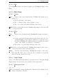
2.5.1
File Menu
2.5.1.1
New
Creates an empty graph in a new tab.
14
2.5. GLuskap Menus
Figure 2.9: Vertex Axes
2.5.1.2
Open . . .
Opens a graph in GLuskap MG or MG2 format. Replaces the current graph
if it is empty and unmodified. Otherwise, creates a new tab.
2.5.1.3
Revert
Reloads the current graph from the filesystem, discarding any changes since
it was last saved. Not possible if the graph was created (i.e. by File—New
and has not yet been saved.
2.5.1.4
Close
Closes the current graph, prompting to save if changes have been made.
2.5.1.5
Save
Saves the graph in GLuskap MG or MG2 format. If the graph has not been
previously saved, opens the Save As window.
2.5.1.6
Save As . . .
Saves the graph in GLuskap MG or MG2 format in a new file or location.
2.5.1.7
Import
Opens a graph saved in an external format (i.e. GraphML or GML). Note
that some features of external formats may not be supported.
15
Using GLuskap
2.5.1.8
Export
As Graph File . . . Saves the graph in an external format (GraphML or
GML).
Note that some features of external formats may not be supported, and
not all external formats support all GLuskap features.
As Image . . . Saves the current Graph Display view as an image file in a
common format. Image formats supported include .png, .jpg, .tif, and
.bmp.
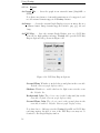
As POV-Ray . . . Save the current Graph Display view as a POV-Ray
scene file for high-quality rendering. GLuskap will open the POV-Ray
Export Options dialog, shown in Figure 2.10.
Figure 2.10: POV-Ray Export Options
Ground Plane Whether to include the ground plane in the scene file.
Default: Current graph display setting
Shadows Whether to enable shadows for light sources in the scene
file. Default: On
Background Color The color to use for the background/sky in the
scene file. Default: Current graph display setting
Ground Plane Color The color to use for the ground plane in the
scene file, if enabled. Default: Current graph display setting
Note that due to differences in the GLuskap/OpenGL and POV-Ray
rendering engines, the field of view of the POV-Ray scene may not be
identical to the Graph Display window.
16
2.5. GLuskap Menus
2.5.1.9
Exit
Closes GLuskap. If there are unsaved graphs open, GLuskap prompts to save
them.
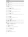
2.5.2
Edit Menu
2.5.2.1
Vertex
New . . . Create a new vertex interactively. GLuskap will prompt, in sequence, for:
• The ID and name of the vertex
• The coordinates of the vertex (Default: origin)
• The color, radius, and initial visibility of the vertex
Delete Delete a vertex interactively. GLuskap will prompt for the vertex ID
to delete from a list.
2.5.2.2
Edge
New . . . Create a new edge interactively. GLuskap will prompt, in sequence,
for:
• A source vertex and an appropriate target vertex for the edge. Recall that GLuskap does not support duplicate or degenerate edges,
and that as GLuskap only supports undirected graphs, the names
“source” and “target” are purely for convenience.
• The radius, color, and initial visibility of the edge.
Delete Delete an edge interactively. GLuskap will prompt for the edge to
delete from a list of source and target pairs.
Bend . . . Bend an edge interactively. GLuskap will prompt for the source
and target ID of the edge to bend and the coordinates to create the
new bend point (default: the origin).
2.5.3
View Menu
Many of the functions in this menu are discussed in 2.4: Using the Graph
Display Panel. Cross-references are indicated where appropriate.
2.5.3.1
Orthogonal View
(See 2.4.4)
Off Use the standard camera allowing three-dimensional movement and arbitrary orientation. (Default)
17
Using GLuskap
Left / Right Use an orthogonal camera with the cameral normal parallel
to the world X axis.
Front / Back Use an orthogonal camera with the cameral normal parallel
to the world Z axis.
Top / Bottom Use an orthogonal camera with the cameral normal parallel
to the world Y axis.
2.5.3.2
Show Ground Plane
Enable/disable the ground plane in the graph view. (See 2.4.1)
2.5.3.3
Show Axes
Enable/disable the world axes in the graph view. (See 2.4.1)
2.5.3.4
Show Vertex Axes
Enable/disable local vertex axes in the graph view for selected vertices. (See
2.4.5)
2.5.3.5
Show HUD
Enable/disable the Heads-Up Display. (See 2.4.2)
2.5.3.6
Vertex Labels
IDs / Names / Off Enable/disable display of vertex IDs or names as vertex labels in the graph display panel.
Bend points If vertex labels are enabled, show/hide labels for bend points.
Label Color / Label Shadow Color Set the color used to draw the vertex label text and the offset shadow.
2.5.3.7
Background Color
Set the background color of the graph display pane.
2.5.3.8
Ground Plane Color
Set the color of the ground plane.
2.5.3.9
Full Screen
Enable/disable GLuskap full screen mode.
18
2.5. GLuskap Menus
2.5.4
Tools Menu
2.5.4.1
Layouts
These layouts are designed to aid in visualizing graphs without vertex positioning information, or as starting points for hand-optimization of vertex
positions.
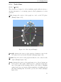
Circle Arranges the vertices of the graph in a circle on the X-Y plane.
(Example figure 2.11)
Figure 2.11: Circle Layout Example
Butterfly Arranges the vertices of the graph in a lemniscate curve in the
X-Y plane and bowed in the X-Z plane. (Example figure 2.12)
Random Place the vertices of the graph randomly in a cube centered at the
origin. (Example figure 2.13)
Spring Arranges the vertices of the graph using a force-directed spring embedder model. The results of this layout are contingent on the structure of the graph and the starting positions of the vertices. GLuskap’s
spring layout uses an iterative physics-simulation algorithm with an
unbounded running time, but tends to produce nice results. (Example
figure 2.14)
19
Using GLuskap
Figure 2.12: Butterfly Layout Example
Figure 2.13: Random Layout Example
20
2.5. GLuskap Menus
Figure 2.14: Spring Layout Example
2.5.4.2
Reflect in Axis
Reflects the entire in the plane of the specified axis; e.g. reflecting in the
plane X=0 negates the X coordinate of all vertices.
2.5.4.3
Flatten in Plane
Flattens the entire graph into the specified plane; e.g. to flatten into the XZ
plane, sets the Y coordinate of all vertices to 0.
2.5.5
Help Menu
2.5.5.1
About
Displays information about the current version of GLuskap, the project, and
contact and copyright information.
21
Using GLuskap
22
Appendix A
MG2 Technical Reference
A.1
Overview
The MG2 file format is a flat text format optimized for storing graph drawings
with a minimum of overhead. MG2 files are relatively easy to read and yet
easy to manipulate with standard text editing and processing tools.
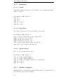
A.1.1
Formal Representation
The structure of MG2 is illustrated by the following EBNF:
hMG2i
hrecordlisti
hrecordi
hrecord-tagi
hfieldi
hfield-datai
hshort-stringi
hquoted-stringi
−→
−→
−→
−→
−→
−→
−→
−→
hrecordlisti
hrecordi hrecordlisti | ε
hrecord-tagi hfieldi + newline
fileformat | vert | dummy | edge | super
hfield-tagi hfield-datai +
integer | real | hshort-stringi | hquoted-stringi
hwordchari + (\ (Ã | ") hwordchari +) ∗
" (hwordchari + (Ã | \") ?) + "
Each record type (indicated by the “record tag”) allows a subset of data
fields to be specified, each denoted by a prefix or “field tag”. Fields can
appear in any order in a record.
Any text following an unquoted # (hash mark, pound sign) on a line is
ignored. This allows MG2 files to be commented.
23
MG2 Technical Reference
A.1.2
Examples
A.1.2.1
Simple
This simple example shows the power of MG2 to create graphs with a minimum of overhead.
fileformat id MG2 version 1
vert id 1
vert id 2
vert id 3
edge src 1 tgt 2
edge src 2 tgt 3
A.1.2.2
Bent Edges
Two vertices connected by an edge with three bend points.
fileformat id MG2 version 1
vert id 1 pos -10.0 0.0 0.0 rgb 1.0 0.0 0.0
dummy id 101 pos -5.0 5.0 0.0
dummy id 102 pos 0.0 0.0 -5.0
dummy id 103 pos 5.0 5.0 -5.0
vert id 2 pos 10.0 0.0 0.0 rgb 1.0 0.0 0.0
super src 1 tgt 2 bend 3 101 102 103
A.1.2.3
Quoted Strings
Like A.1.2.1, but with named vertices
fileformat id MG2 version 1
vert id 1 name vertex_number_1
vert id 2 name "Vertex Number 2"
vert id 3 name "Including a quote (\") character"
edge src 1 tgt 2
edge src 2 tgt 3
A.1.3
Further examples
GLuskap includes several sample graphs in MG2 format. See Appendix B for
more information about these samples.
24
A.2. Record Description Format
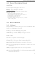
A.2
Record Description Format
record-taga
A brief description of the purpose of the record.
field-tag
b
(type)c Description of the field.
a
The record tag is an alpha string with no whitespace indicating the type of the record.
b
The field tag is an alpha string with no spaces.
c
The data format for the field is given as a list of types, e.g.
• (string) indicates a single string value.
• (int int int) indicates three integers.
• (int string+) indicates an integer followed by a variable
number of string values.
A.3
A.3.1
Record Formats
fileformat
The fileformat record indicates the type and version of the MG2 file. There
should be one fileformat record per file.
id The type of the file. GLuskap supports type MG2.
version The type of the file. GLuskap 2.4.x supports version 1.
A.3.2
vert
The vert record specifies a vertex in the graph.
id (string) The id of the vertex. Must be unique within the file.
name (string) (Optional) Description or annotation of the vertex.
pos (real real real) (Optional) The 3-dimensional coordinates of the center
of the vertex.
radius (real) (Optional) The radius of the vertex representation.
rgb (real real real) (Optional) The color of the vertex representation as RGB
values in the range [0.0, 1.0].
25
MG2 Technical Reference
A.3.3
dummy
The dummy record specifies a dummy vertex which must be listed as a bend
point in a super record. The fields for a dummy record are identical to the
vert record fields.
A.3.4
edge
The edge record specifies an edge in the graph. The source and target of the
edge must be a unique pair of distinct vertices.
src (string) The id of the source vertex of the edge.
tgt (string) The id of the target vertex of the edge.
radius (real) (Optional) The radius of the edge representation.
rgb (real real real) (Optional) The color of the edge as RGB values in the
range [0.0, 1.0].
attr (string) (Optional) Description or annotation of the edge.
A.3.5
super
The super record specifies a superedge, i.e. an edge described by a polyline. A super record has all the fields of an edge record, with the following
addition:
bend (int string+) The number of bend points in the edge followed by the
IDs of the dummy vertices making up the bend points. dummy records
must exist for all bend points specified in a bend record.
By default, the subedges will be instantiated automatically with the properties of the superedge. If some or all of the subedges are specified as edge
records, the properties explicitly defined in those records will be used.
26
Appendix B
Included Sample Graphs
The GLuskap distribution includes a set of sample graphs, located in the
samples directory of the GLuskap installation.
B.1
Samples in MG2 Format
ortho-k7.mg2 K7 arranged orthogonally with no crossings; vertices and
bend points occupy integer grid points and edges follow straight lines
parallel to the world axes.
1-bend.mg2 Sample 1-bend drawing of K8,8 .
goodsoc2.mg2 Used in a submission to Graph Drawing Contest 2003.
spring-world.mg2 A graph representing the geographical connections between all the countries on Earth, arranged by the GLuskap spring embedding arrangement. Used in a submission to Graph Drawing Contest
2004.
B.2
Samples in External Formats
outerplanar.xml An outer planar graph in GraphML format.
ortho-k7.gml Like ortho-k7.mg2, but in GML format.
27
Included Sample Graphs
28