Download Project Manual

SNA: A tool for Stochastic Network Analysis
(CE737 Course Project)
Shahrzad Azizzadeh
5/5/2010
Abstract
This document is the user manual to the SNA: Stochastic Network
Analysis tool. It provides complete information on how to use the system
as well as description of tools and algorithms which are provided in the
software. The Examples provided in this tutorial are all tested properly
by the software.
1
Contents
1
Introduction
3
2
SNA's Technology Dependencies
4
SNA Network Basics
5
3
4
3.1 How to Create a network . . . . . . . . . . . . . . . . . . .
3.1.1 Creating a network manually . . . . . . . . . . . . .
3.1.2 Reading a network from le . . . . . . . . . . . . . .
Working with algorithms
4.1
4.2
4.3
4.4
Connectivity . . . . . . . . . .
Shortest Path . . . . . . . . . .
Max Flow . . . . . . . . . . . .
Capacity Reliability Estimation
.
.
.
.
.
.
.
.
.
.
.
.
.
.
.
.
.
.
.
.
.
.
.
.
.
.
.
.
.
.
.
.
.
.
.
.
.
.
.
.
.
.
.
.
.
.
.
.
.
.
.
.
.
.
.
.
.
.
.
.
.
.
.
.
5
5
6
7
7
7
8
8
5
Network Visulalization
6
An extended example
10
How to install the project
12
Appendix 1:A Sample Data set
12
7
8
9
7.1 Run on Windows . . . . . . . . . . . . . . . . . . . . . . . . 12
7.2 Run on Linux . . . . . . . . . . . . . . . . . . . . . . . . . . 12
2
1
Introduction
SNA is a software for stochastic ow network analysis. It enables the user to accomplish basic and more advanced network analysis under uncertain conditions.
The software is designed and implemented for audiences majoring in math and
engineering. Background on network and graph analysis will help in using the
system, but the manual is complete enough to help the users not familiar with
graph theory as well.
Stochastic network analysis is used to describe the behavior of many complex systems including lifeline networks.
The analysis of the performance of
such networks should be done under uncertainty. Uncertainties stem from the
natural variations in the availability of network components and due to failures,
degradations. Also in real world networks, usually partial information is provided about the demand in the system and it may also follow a distribution other
than being a completely known value. These issues reveal the need to a tool
which gives the opportunity to perform network analysis under uncertainties.
In addition to the basic famous network analysis problems such as shortest
path and connectivity analysis, this tool estimates more advance network metrics such as capacity reliability of the system under uncertainties conditions.
Also this tool provides good visualization capabilities.
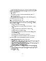
The software is based on two dierent yet interacting tools:
•
Monte Carlo Simulation
•
Network Analysis tool
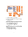
The uncertainty analysis is done by means of Monte Carlo simulation.
The
results of the simulations are passed to the network analysis tool as the input
data.
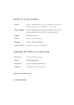
The following gure depicts the high level architecture of SNA.
3
Jung Lib
SP
Distance
Shortest Path
Flow
Graph
Generator
Property File
Key Value
XML
Common
DBGraph
<XML>
2
Terminal
UI
Max Flow
Swing
SP
Flow
Random Factory
Node
Capacitated Link
Capacitated Network
Graph
Alg
Simulator
Graph
Math Lib
DB
Graph
SNA's Technology Dependencies
SNA depends on two java libraries: Commons Math 2.1 API and Jung 2.0 (
Java Universal Network/Graph).
• Commons Math API:
This library is used for generating random numbers from some of the famous
probability distribution functions. The library is available for free download at
:
http://commons.apache.org/math/download_math.cgi
and the javadoc of the library is reachable at :
http://commons.apache.org/math/api-2.1/index.html
• JUNG 2.0:
Graph and network classes of SNA extend some of the classes of this library.
Also it is used for graph visualizations in SNA. The library is available for free
download at :
http://jung.sourceforge.net/doc/index.html
and the javadoc of the library is reachable at :
http://jung.sourceforge.net/doc/api/index.html
4
3
SNA Network Basics
SNA is an object oriented software. It represents a network as a directed graph
which has been read through its incidence matrix. Although SNA uses some of
the classes and interfaces of JUNG and JGRAPHT libraries, it introduces its
own classes for a lot of objects needed for its specic purposes. The structure
of a network in SNA is briey introduced in the following. For a more complete
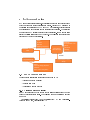
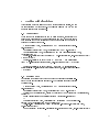
list of the classes please see the SNA javadoc. The following gure depicts the
high level SNA network architecture.
Fields :
Id,Name
Methods:
ToString,Compare to
Node
Capacitated
NetworkGraph
Methods :
Demand Setter and
getters
getVertex
getEdge
Extends
Capacitated Link
Directed Sparse Multi
Graph
Fields :
Capacity,Weight,Id,Name
Methods:
Fields setters and getters
3.1
How to Create a network
There are three alternatives for forming a network in SNA :
•
Creating a network manually
•
Reading from a le
•
Generating a random network
3.1.1 Creating a network manually
In SNA nodes should be of the dened Node class and links should be of the
dened CapacitatedLink class.
The following command initiates a network
named g :
CapacitatedNetworkGraph<Node, CapacitatedLink> g = new CapacitatedNetworkGraph<Node, CapacitatedLink>();
5
As class CapacitatedNetworkGraph of SNA extends the DirectedOrderedSparseMultigraph of Jung library, it inherits its methods, so you can add a node with
the id i to your network by :
g.addVertex(i);
You can also add an edge
e
to between nodes source and sink by :
g.addEdge(e, source, sink);
For a complete set of commands like setting the link distributions, demand
and etc , please see the javadoc of SNA.
3.1.2 Reading a network from le
In this method creating the network begins by dening a properties le. You
need to determine the following to be able to form your network. The names
between are key values.
•
Graph_Nodes : Set of Graph Nodes.
•
Random_Capacity :
Your graph capacity data is random ?
True or
False.
•
Graph_Capacity : If the data is not random provide it here.
•
Graph_Weight : Edge weights go here.
•
Probability_Distribution: If the capacity data is probabilistic, provide
the distributions here.
•
Demand_Mean: The mean of demand of the network
•
Demand_Sigma : The standard deviation of demand of the network
Here is a sample set of data for properties le of a network with 5 nodes :
Graph_Nodes =(Node0, Node1, Node2 , Node3, Node4)
Random_Capacity = True
Graph_Capacity={(Null,6,Null,Null,Null);(Null,Null,3,3,Null);(Null,Null,Null,3,Null);
(Null,Null,Null,Null,6);(Null,Null,Null,Null,Null)}
Graph_Weight={(Null,1,Null,Null,Null);(Null,Null,1,2,Null);(Null,Null,Null,1,Null);
(Null,Null,Null,Null,4);(Null,Null,Null,Null,Null)}
(Comment :N:Normal,E=Exponential,U=uniform)
Probability_Distribution = {(Null,N[6-1],Null,Null,Null);(Null,Null,U[2-4],U[24],Null);
(Null,Null,Null,E[3],Null);(Null,Null,Null,Null,N[6-1]);(Null,Null,Null,Null,Null)}
Demand_Mean = 2.5
Demand_Sigma = 0.5
6
4
Working with algorithms
After creating a network using one of the methods introduced earlier, you can
try some algorithm on your network. The following will show you how you can
run these algotithms in the software.
4.1
Connectivity
There are a lot of explorations you can do using this tool , connectivity of a
pair of node, connectivity of the over all network and etc. As an example we
have provided the code to investigate whether a given node of the network is
connected to all the other nodes.
GraphGenerator<Node, CapacitatedLink> gg = PropertyFileGraphGenerator.getInstance();
CapacitatedNetworkGraph<Node, CapacitatedLink> cng = gg.getGraph();
ConnectivityLabeler<Node, CapacitatedLink> cl = new ConnectivityLabeler<Node,
CapacitatedLink>();
System.out.println("Is Graph Connected : " + ((cl.isConnected(cng, cng.getVertex(fromNode))
? "Yes" : "No")));
System.out.println("Number of Nodes " + fromNode + " is disconnected
from : " + cl.disconnectedNodesCount(cng, cng.getVertex(fromNode)) + " Nodes");
System.out.println("Number of Nodes " + fromNode + " is directly disconnected from : " + cl.disconnectedNodesDirectlyCount(cng, cng.getVertex(fromNode))
+ " Nodes");
4.2
Shortest Path
To calculate the shortest path between a pair of nodes using Dijkastra's algorithm you can use the following sample code. The transformer is used to return
the links weight.
GraphGenerator<Node, CapacitatedLink> gg = PropertyFileGraphGenerator.getInstance();
CapacitatedNetworkGraph<Node, CapacitatedLink> cng = gg.getGraph();
Transformer<CapacitatedLink, Double> wTransformer = new Transformer<CapacitatedLink,
Double>() {
public Double transform(CapacitatedLink link) { return link.getWeight(); }
};
DijkstraShortestPath<Node, CapacitatedLink> spAlgorithm = new DijkstraShortestPath<Node, CapacitatedLink>(cng, wTransformer);
java.util.List<CapacitatedLink> path = spAlgorithm.getPath(cng.getVertex(fromNode),
cng.getVertex(toNode));
Number distance = spAlgorithm.getDistance(cng.getVertex(fromNode), cng.getVertex(toNode));
7
System.out.println(" Distance from :" + "Node-" + fromNode + " to " +
toNode + " is : " + distance);
System.out.println(" Path from :" + "Node-" + fromNode + " to " + toNode
+ " is : " + path);
4.3
Max Flow
To calculate the maximum ow passing through a pair of nodes considering the
link capacities the sofware uses Edmonds Karp algorithm which is an implementation of Ford Folkerson method. You can use the following sample code to
calculate the max ow on your network between desired nodes.
GraphGenerator<Node, CapacitatedLink> gg = PropertyFileGraphGenerator.getInstance();
CapacitatedNetworkGraph<Node, CapacitatedLink> cng = gg.getGraph();
Transformer<CapacitatedLink, Double> capTransformer = new Transformer<CapacitatedLink,
Double>() {
public Double transform(CapacitatedLink link) { return link.getCapacity();
} };
Map<CapacitatedLink, Double> edgeFlowMap = new HashMap<CapacitatedLink,
Double>();
// This Factory produces new edges for use by the algorithm
Factory<CapacitatedLink> edgeFactory = new Factory<CapacitatedLink>()
{
public CapacitatedLink create() { return new CapacitatedLink(1, 1.0, 1.0);
} };
try { EdmondsKarpMaxFlow<Node, CapacitatedLink> maxFlowAlgorithm
= new EdmondsKarpMaxFlow(cng, cng.getVertex(fromNode), cng.getVertex(toNode),
capTransformer,
edgeFlowMap, edgeFactory); maxFlowAlgorithm.evaluate();
System.out.println(" Maximum Flow from :" + "Node-" + fromNode + " to
" + toNode + " is : " +
maxFlowAlgorithm.getMaxFlow()); }
catch (IllegalArgumentException e) {
System.out.println(" Maximum Flow from :" + "Node-" + fromNode + " to
" + toNode + " is : No Flow"); }
4.4
Capacity Reliability Estimation
The capacity reliability estimation method has the following steps :
1. Sampling from all the link capacities
2. Calculating the Max Flow of the network using the data provided in step
1.
8
3. Sample the demand from its distribution
4. Comparing the demand and the maximum ow
5. For the desired number of iterations do steps 1-4
6. return the percentage of times the maximum ow the network is able to
provide exceedes the demand.
You can use the following commands to run such a simulation for 1000 times
for the ow between your hypothetical 0 and 4 nodes and get the results.
GraphGenerator graphGenerator = PropertyFileGraphGenerator.getInstance();
ReliabilityEvaluation re = new ReliabilityEvaluation(1000);
System.out.println("Capacity Reliability Estimation" + re.estimate(graphGenerator,
0, 4));
5
Network Visulalization
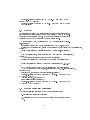
By now, you have created your desired graph and implemented some algorithms.
SNA also gives the ability to visualize your work. SNA's network visualization
takes advantage of the great visual features of Jung library. You can use the
Visual Demo class in SNA as a user interface for implementing most of the
algorithms discussed so far.
Here is a sample view of what SNA is able to
provide.
9
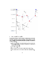
6
An extended example
Implementation of all the methods and algorithms available through the software
is provided here using an extended example.
As all the necessary commands
have been discussed in the previous sections, here we only introduce a case for
which the creating is via reading from le and implementing the algorithm is
by using the interface.
1. Create a properties le in your project directory, the name of the le can
be :
exam1.properties .
The sample of the le for a 15 node graph is
provided in the appendix.
2. Run Visula Demo.java le
3. From the rst combo box choose the desired source (origin) node.
4. From the second combo box choose the desired sink (destination) node.
10
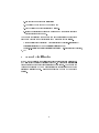
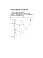
5. The sofware will calculate and return the followings :
(a) Minimum Distance between the node pair
(b) Maximum Flow between the node pair
(c) If the node is connected to all other nodes of the network
6. By clicking on the CapRelEst the program will run a simulation and
returns the capacity reliability estimation.
7. Here is how the result look like for the sample graph at one of the runs:
11
7
How to install the project
To run the program on Windows or Linux you need to have java run time
environment (JRE) 1.6+ installed. To install the project download the binary
les at the following address:
http://www4.ncsu.edu/~sazizza/737/project/sna/sna-1_0_source.jar
unzip the compressed le into a folder.
7.1
Run on Windows
Before running the project on windows set the JAVA_HOME in windows Environment Variables or open run.bat with notepad and change the line pointing
to your java home directory by removing REM from the following statement.
For example change
REM set JAVA_HOME=C:\Program Files\Java\jdk1.6.0_18
to
set JAVA_HOME=<YOUR JAVA HOME DIRECTORY>
after modifying run.bat le, simply execute the le by double clicking or
using Command Prompt.
7.2
Run on Linux
Make sure that JRE 1.6+ is installed and java bin directory is added to system
PATH variables then run.sh by either one of these commands:
./run.sh
sh run.sh
8
Appendix 1:A Sample Data set
Sample properties le data set for the discussed network:
Comments#15NodeConnectedNetwork
#N:Normal,E=Exponential,U=uniform
Probability_Distribution=
{(Null,U[0-3],N[10-1.5],Null,Null,Null,Null,Null,Null,Null,Null,Null,Null,Null,Null);(U[03],Null,N[8-1],Null,Null,Null,Null,Null,Null,Null,Null,Null,Null,Null,Null);(Null,Null,Null,N[182],Null,Null,Null,Null,Null,Null,Null,Null,Null,Null,Null);(Null,Null,Null,Null,N[30.5],Null,N[3-0.5],Null,N[12-2],Null,Null,Null,Null,Null,Null);(Null,Null,Null,Null,Null,E[31],Null,N[2-0.25],Null,Null,Null,Null,Null,Null,Null);(Null,Null,Null,Null,Null,Null,Null,E[31],Null,Null,Null,Null,Null,Null,Null);(Null,Null,Null,Null,Null,Null,Null,Null,N[30.5],N[3-0.5],Null,Null,Null,Null,Null);(Null,Null,Null,Null,Null,Null,Null,Null,Null,Null,N[31],Null,Null,Null,Null);(Null,Null,Null,Null,Null,Null,N[3-0.5],N[5-1],Null,U[3-6],Null,N[6-
12
2],Null,N[7-2],N[8-1]);(Null,Null,Null,Null,Null,Null,Null,Null,U[3-6],Null,Null,N[51],Null,Null,Null);(Null,Null,Null,Null,Null,Null,Null,Null,Null,Null,Null,Null,N[30.5],N[2-0.25],Null);(Null,Null,Null,Null,Null,Null,Null,Null,Null,Null,Null,Null,Null,Null,U[2-
4]);(Null,Null,Null,Null,Null,Null,Null,Null,Null,Null,Null,Null,Null,Null,Null);(Null,Null,Null,Null,Null,Null,N
2]);(Null,Null,Null,Null,Null,Null,Null,Null,Null,Null,Null,Null,Null,N[18-2],Null)}
Graph_Capacity=
{(Null,1,2,Null,Null,Null,Null,Null,Null,Null,Null,Null,Null,Null,Null);(1,Null,2,Null,Null,Null,Null,Null,Nu
Graph_Weight= {(Null,1,2,Null,Null,Null,Null,Null,Null,Null,Null,Null,Null,Null,Null);(1,Null,2,Null,Null,
Graph_Nodes =(Node0, Node1, Node2 , Node3, Node4,Node5, Node6, Node7
, Node8, Node9,Node10, Node11, Node12 , Node13, Node14)
13