Download SEAWAT 4 Tutorial

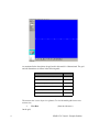
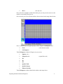
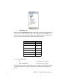
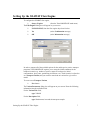
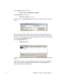
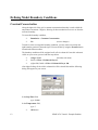
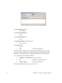
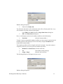
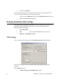
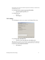
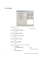
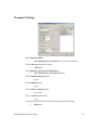
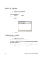
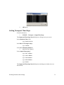
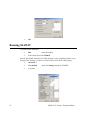
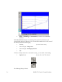
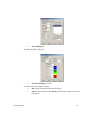
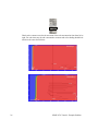
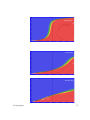
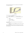
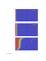
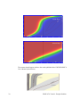
SEAWAT 4 Tutorial - Example Problem
Introduction
About SEAWAT-4
SEAWAT-4 is the latest release of SEAWAT computer program for simulation of threedimensional, variable-density, transient ground-water flow in porous media. SEAWAT
was originally designed by combining a modified version of MODFLOW-2000 and
MT3DMS into a single computer program. SEAWAT-4 includes all of the capabilities
of previous versions with the addition of some new features, including:
• The ability to simulate heat and solute transport simultaneously.
• The ability to simulate the effect that fluid viscosity variations have on
resistance to ground-water flow using the Viscosity (VSC) Package.
• Simulate fluid density as a function of temperature and one or more MT3DMS
species and, optionally, a pressure term. You can also specify one of several
non-linear equations to represent the dependence of viscosity on temperature.
• For the Time-Variant Constant-Head (CHD) package, auxiliary variables can
now be used to designate the fluid density value associated with the prescribed
head.
Sample Applications
Some examples of applications for SEAWAT-4 include:
• Simulating the transport of heat and salinity in coastal aquifers, and thermally
driven convection in deep aquifers
• ASR: Storage of freshwater in saline aquifers: simulate buoyancy effects, and
the affect of groundwater temperature on the fluid viscosity.
• Geothermal investigations - The heat balance calculation and the impact of
groundwater heat pumps on the groundwater temperature
• Affect of volcanic activities on groundwater and the water table
• Fate of wastewater injected into deep wells, and impact on the aquifer
Background
This tutorial assumes that you are already familiar with the Visual MODFLOW
interface, and with the process of building a groundwater model. If you are not familiar
with Visual MODFLOW, it is recommended that you work through the Visual
MODFLOW tutorial first.
Introduction
1
This tutorial illustrates a common application for SEAWAT and is based on the
Example Problem: Case 7 published in User’s Guide to SEAWAT 4. Please note that
output results may vary slightly from published results as this model has been scaled
down to allow for shorter run times.
The problem consists of a two-dimensional cross section of a confined coastal aquifer
initially saturated with relatively cold seawater at a temperature of 5°C. Warmer
freshwater with a temperature of 25°C is injected into the coastal aquifer along the left
boundary to represent flow from inland areas. The warmer freshwater flows to the right,
where it discharges into a vertical ocean boundary. The ocean boundary is represented
with hydrostatic conditions based on a fluid density calculated from seawater salinities
at 5°C. No flow conditions are assigned to the top and bottom boundaries.
Reference: Langevin, C.D. Thorne, D.T., Jr., Dausman, A.M., Sukop, M.C., and Guo,
Weixing, 2008, SEAWAT Version 4: A Computer Program for Simulation of MultiSpecies Solute and Heat Transport: U.S. Geological Survey Techniques and Methods
Book 6, Chapter A22, 39 p.
Terms and Notations
For the purposes of this tutorial, the following terms and notations will be used:
Type: - type in the given word or value
Ù - press the Tab key on your keyboard
<Enter> - press the Enter key on your keyboard
) - click the left mouse button where indicated
)) - double-click the left mouse button where indicated
The bold faced type indicates menu or window items to click on or values to type in.
[...]
- denotes a button to click on, either in a window, or in the side or bottom
menu bars.
Opening the Visual MODFLOW Model
For your convenience, part of the model has already been prepared for you. The Visual
MODFLOW project file is located on your computer and can be opened by following
the directions below.
A full version of the model following this step-by-step tutorial has already been created
and is located on the FTP site. To download the full version of the model, please visit
the following ftp address:
ftp://ftp.flowpath.com/Software/VMOD/2010.1/Tutorials
2
SEAWAT 4 Tutorial - Example Problem
NOTE: Some features described in this tutorial are only available in a Standard +
SEAWAT, Pro or Premium version. If you are using a standard version of VMOD and
wish to upgrade your software, please contact [email protected]
On your Windows desktop, you will see an icon for Visual MODFLOW.
))
Visual MODFLOW to start the program
To open the model:
)
File
)
Open
(from the top menu bar)
An Open Visual MODFLOW file window will appear.
Navigate to the following directory on your computer:
C:\My Documents\Visual MODFLOW\Tutorials\Seawat_Heat
)
Seawat4_Tutorial.vmf
)
Open
Next, you will take a quick look at some aspects of the model that have already been
prepared for you. After that, we will create a new SEAWAT variant for simulating heat
and salt transport.
Exploring the Model Grid and Properties
In this section, you will explore some aspects of the model that have already been
defined for you, such as the model grid and properties. This information can be viewed
in the Input window,
)
Input
Exploring the Model Grid and Properties
(from the Visual MODFLOW main menu)
3
As mentioned in the description, the grid used in this model is 2-dimensional. The grid
and cell dimensions are shown in the following table.
Input Parameter
Value
Number of Columns (NCOL)
100
Number of Rows (NROW)
1
Number of Layers (NLAY)
100
∆x (DELR)
10m
∆y (DELC)
1m
∆z (DZ)
10m
Table 1: Model grid and cell dimensions
The current view is set to layer view (planar). To view the model grid from a cross
section view,
)
View Row
(from the side menu )
On the grid,
4
SEAWAT 4 Tutorial - Example Problem
)
Row 1
(the only row)
Due to the ratio of length to width of the model grid, you may need to zoom in on the
model to successfully select the row.
Once selected, your view will look similar to the one shown in the image shown below.
Next, we will look at the assigned property values using the Cell Inspector tool.
)
Tools
)
Cell Inspector
(from the main menu)
The Cell Inspector window will appear on your screen.
)
Options ( tab )
)
Properties node
)
Kx
)
Ky
)
Kz
)
Specific Yield
)
Specific Storage
)
Effective Porosity
(expand this node)
The Cell Inspector window should look similar to the image below.
Exploring the Model Grid and Properties
5
)
Cell Values ( tab )
While leaving the Cell Inspector window opened, move your mouse across the cells in
the grid. You will see the assigned property values populate in the Cell Inspector
window. Also, you will notice that all properties are uniform across the entire model
grid. The values for each property are shown in the following table:
Property
Value
Kx
10 m/d
Ky
10 m/d
Kz
0.1 m/d
Specific Yield
1
Specific Storage
1e-05 1/m
Effective Porosity
0.35
Table 2: Assigned property values
To close the Cell Inspector,
)
X
(top-right corner of window )
)
File > Main Menu
(from the Input main menu)
The next section will guide you through the steps of setting up a SEAWAT flow engine
including the creation of a transport variant that contains both salt and temperature
species.
6
SEAWAT 4 Tutorial - Example Problem
Setting Up the SEAWAT Flow Engine
To configure the SEAWAT flow engine,
)
Setup > Engines
(from the Visual MODFLOW main menu)
The Edit Engines dialog box will appear on your screen.
)
USGS SEAWAT, from the flow engine drop down list box
)
Yes
(at the Confirmation message)
)
OK
(at the Information message)
In order to support all of the available options for the multi-species reactive transport
programs, Visual MODFLOW requires you to setup the initial conditions for the
transport scenario (e.g. number of species, names of each species, initial
concentrations, decay rates, partitioning coefficients, etc.). Each scenario is referred to
as a Transport Variant, and you can have more than one variant for a given flow
model.
To create a new Transport Variant,
)
New button
The Variant Parameters dialog box will appear on your screen. Enter the following
information into the available fields:
For the Variant Title field,
type: VAR002
For the Description field,
type: Simultaneous heat and salt transport example
Setting Up the SEAWAT Flow Engine
7
For the Sorption drop down list box,
)
Linear Isotherm (equilibrium-controlled)
For the Reactions drop down list,
)
No kinetic reactions (leave as is)
The top half of the Variant Parameters dialog box show appear similar to the image
below:
Next, you will specify the appropriate parameters for the variant parameters. In the
bottom half of the dialog, you will see that, by default, the Salt species already exists.
However, in order to simulate heat transport simultaneously with solute (salt) transport,
you need to add a Temperature species.
To add a Temperature species,
)
Temperature button
For both the Salt and Temperature species, you can now enter the appropriate parameter
values.
For the Salt species (row 1) type the following parameter values into the appropriate
fields under the Species or Species Params tab. Note: The Species Params tab
contains descriptions of each parameter.
8
SEAWAT 4 Tutorial - Example Problem
Parameter
Value
SCONC (mg/L)
35000
SP1 (1/mg/L)
0
DRHODC
0.7
CREF (mg/L)
0
MDCOEF (m2/Day)
1e-10
DMUDC (m2/Day)
1.923e-6
Table 3: Variant parameter values for salt species
Once these values have been entered, under the Species tab, set the Temperature
species to mobile,
)
Yes, under the Mobile column for the Temperature species.
For the Temperature species, type the following parameter values into the appropriate
fields under the Species or Species Params tab.
Parameter
Value
SCONC(mg/L)
5
SP1 (1/mg/L)
2e-7
DRHODC
-0.375
CREF (mg/L)
25
MDCOEF (m2/Day)
0.15
DMUDC (m4/Day)
0
Table 4: Variant parameter values for temperature.
The next step is to enter the appropriate model parameters.
)
Model Param tab
Visual MODFLOW provides typical values for various model parameters. In the
corresponding fields, modify the following parameters according to the values in the
table below:
Setting Up the SEAWAT Flow Engine
9
Parameter
Value
RHOB (Bulk Density (kg/m^3))
1760
DENSEMIN (Minimum Fluid Density)
0
DESNMAX (Maximum Fluid Density)
0
DENSESLP (Density/Concentration Slope)
0.7
VISCMIN (Minimum Fluid Viscosity)
0
VISCMAX (Maximum Fluid Viscosity)
0
Table 5: Constant Variant Model Parameters
The default values for the remaining parameters are acceptable.
Now that all the parameters have been defined, we can create the variant.
)
OK button
)
OK button
(at the Edit Engines window)
Editing Dispersion Properties
)
Input from the main menu
)
Properties > Dispersion
)
Layer Options from the side menu
The Dispersion Package window will appear on your screen.
In the empty field above the Vert/Long Dispersivity column,
type: 0.1
10
SEAWAT 4 Tutorial - Example Problem
)
OK button
)
Database
(from the side menu)
The Dispersion window will appear on your screen.
In the DI(m) field,
type: 1
)
OK button
Setting Up the SEAWAT Flow Engine
11
Defining Model Boundary Conditions
Constant Concentration
Along the right side of the grid, a constant concentration boundary is used to hold the
temperature constant at 5 degrees, allowing for heat conduction to occur to or from the
seawater boundary.
To create this boundary condition,
)
Boundaries > Constant Concentration
)
Yes
(to save changes)
To make it easier to assign this boundary condition, you may want to zoom into the
right boundary portion of the model grid. You can do this by using the Zoom In button
located at the bottom toolbar.
The boundary condition will be assigned to all cells in column 99. Once this column is
visible on your screen, proceed with the steps below.
)
Assign > Line
)
Inside cell Row 1 Column 99 Layer 1
)
(right-click) Inside cell Row 1 Column 99 Layer 100
(from the side menu)
After right-clicking, all the cells in column 99 will be colored blue and the following
dialog will appear on your screen:
In the Stop Time field,
type: 200000
In the Temperature field,
type: 5
)
12
OK button
SEAWAT 4 Tutorial - Example Problem
Point Source
The next step is to assign point source concentrations at both the left and right
boundaries. However, because point source concentrations must be associated with a
flow boundary, you must assign the appropriate flow boundaries first.
On the left boundary, the well package is used to define an inflow of water from the
boundary. For your convenience, the well boundary has already been assigned for you.
To view the well boundary, follow the steps below.
If you are currently zoomed in,
)
Zoom Out
(located at the bottom tool bar )
When you see the full grid on your screen,
)
Wells > Pumping, from the menu bar.
)
Yes
(at the Save message)
At the left boundary, you will see that a well boundary condition has been defined.
From the left side bar,
)
Database button
The Edit Well window will appear on your screen. Here you can see for PW001 a
pumping rate (injection) of 10 m3/d has been assigned to the entire column, resulting in
a rate 0.1 m3/day at each individual cell.
)
OK
(to close the Edit Well window.)
Along the right boundary, we will assign a Constant Head flow boundary condition.
To make it easier to assign this boundary condition, you may want to zoom into the
right boundary portion of the model grid. You can do this by using the Zoom In button
located at the bottom toolbar.
The boundary condition will be assigned to all cells in column 100. Once this column is
visible on your screen, proceed with the steps below.
)
Boundaries > Constant Head
(from the menu bar)
)
Assign > Line
(from the side menu bar)
)
Inside cell Row 1 Column 100 Layer 1
)
Inside cell Row 1 Column 100 Layer 100
)
Right-click in cell Row 1 Column 100 Layer 100
Upon right-clicking, all cells in column 100 will be colored pink, and the following
dialog box will appear on your screen.
Defining Model Boundary Conditions
13
In the Stop Time (day) field,
type: 200000
In the Start Time Head field,
type: 0
In the Stop Time Head field,
type: 0
In the Density Options drop down list box,
)
No Conversion
In the Density field,
type: 0
)
OK
(to close the dialog box)
Now that the flow conditions have been assigned at each boundary, you can now
proceed to define the point source boundary conditions. We will start at the right
boundary, as you should already be zoomed into that portion of the model grid.
To assign a point source boundary condition,
)
Boundaries > Point Source (from the menu bar)
)
Yes
(at the Save warning message)
)
Assign > Single
(from the side bar menu)
The following dialog box will appear on your screen:
14
SEAWAT 4 Tutorial - Example Problem
With the dialog still opened,
)
Each cell in Column 100
You will notice that when a cell is clicked, the color of the cell turns pink. Once every
cell in column 1 has been selected (colored pink),
type: 35000, in the Salt field of the Assign Point Source dialog box
)
OK, in the Point Source dialog box.
Next, we will assign a point source boundary condition to the left boundary.
)
Zoom Out
(from the bottom toolbar. )
To make it easier to assign this boundary condition, you may want to zoom into the left
boundary portion of the model grid. You can do this by using the Zoom In button
located at the bottom toolbar.
The boundary condition will be assigned to all cells in column 1. Once this column is
completely visible on your screen, proceed with the steps below.
)
Boundaries > Point Source (from the menu bar)
)
Yes
(at the Save warning message)
)
Assign > Single
(from the side bar menu)
The following dialog box will appear on your screen:
With the dialog still opened,
Defining Model Boundary Conditions
15
)
Each cell in Column 1
You will notice that when a cell is clicked, the color of the cell will turn pink. Once
every cell in column 200 has been clicked (colored pink),
type: 25, in the Temperature field of the Assign Point Source dialog box.
)
OK, in the Point Source dialog box.
Defining Simulation Run Settings
Now that the grid, properties and boundaries have been defined, you can proceed to
translate and run the SEAWAT model. However, first you must configure the
appropriate simulation settings.
)
File >Main Menu
)
Run
)
SEAWAT > Simulation Scenario
(from the Visual MODFLOW main menu bar)
VDF Settings
First you will define the settings for the Variable Density Flow (VDF) package.
For the VDF Package, most of the default values are acceptable, except for the
following:
Under Density Scenario,
)
16
Calculate density from multiple species option
SEAWAT 4 Tutorial - Example Problem
Selecting this option will ensure that both temperature and salinity are included when
calculating density values.
Under Internodal density calculation algorithm [MFNADVFD],
)
Upstream-weighted algorithm option
Under Initial Time Step,
type: 0.01
)
VSC Settings tab
VSC Settings
The VSC Settings tab contains various options for the Viscosity (VSC) package.
Under Viscosity Option [MT3DMUFLG],
)
Calculate viscosity from temperature and multiple species
When this option is selected, you can select from various parametrization options for
calculating the temperature term in the viscosity equation. In this case, we will retain
the default setting, Voss (1984) Parametrization.
)
Flow Settings tab
Defining Simulation Run Settings
17
Flow Settings
For the Solver,
)
PCG option
(along the left side)
For Max. outer iterations (MXITER)
type: 100
For Max. inner iterations (ITER1)
type: 25
For Head change criterion (HCLOSE)
type: 1e-5
For Residual criterion (RCLOSE)
type: 1
For Printout interval (IPRPCG)
type: 5
Finally, under package options (top right corner of dialog)
18
)
User Defined
)
+ Specified Head Package
(node)
)
Run
(to unselect the checkbox)
)
Transport Settings tab
SEAWAT 4 Tutorial - Example Problem
Transport Settings
Under Solution Options,
)
Solve Implicitly (Use GCG Solver), to unselect the checkbox
For the Advection drop down list box,
)
TVD option
Under Dispersion, Reaction and Sink/Sources,
)
Solve Implicitly (Use GCG Solver) option
For the Maximum Step Size field,
type: 0
For the Multipler field,
type: 1
For the Min. sat. thickness field,
type: 5e-02
For the Courant number field,
type: 1
To accept all modifications and close the Simulation Scenario window,
)
OK button
Defining Simulation Run Settings
19
Setting Flow Time Steps
From main menu,
)
SEAWAT > Flow > Time Steps
The Time Step Options dialog will appear on your screen.
For the Time Steps field,
type: 10
(default)
For the Multiplier field,
type: 1
)
OK button
Configuring Layer Settings
From main menu,
)
SEAWAT > Flow > Layers
The Layer Settings dialog will appear on your screen.
For each layer, change the layer type from 3:Confined/Unconfined, variable S,T to
0:Confined, Constant S, T.
To save time, you can select all the rows by clicking and dragging your mouse along the
left side of the grid. Once all the rows are selected, you can select 0:Confined,
Constant S,T. from the drop down list box at the top of the window.
20
SEAWAT 4 Tutorial - Example Problem
)
OK button
Setting Transport Time Steps
From the main menu,
)
SEAWAT > Transport > Output/Time Steps
The Output and Time Step Control dialog box will appear on your screen.
In the Simulation Time field,
type: 200000 (default)
In the Max # of Transport Steps,
type: 1000000
Under Save Simulation Results at,
)
Specified Time [day(s)]
Under Output Time(s)[day]
type: 5000 <Enter>
type: 10000 <Enter>
type: 30000 <Enter>
type: 60000 <Enter>
type: 200000
The Output and Time Step Control dialog box should appear similar to the one
shown below.
Defining Simulation Run Settings
21
)
OK
Running SEAWAT
To run the model simulation,
)
Run
)
In the check box beside SEAWAT
(from the toolbar)
Because the Variable Density Flow (VDF) package is only compatible with the Layer
Property Flow Package, you have to set the model to run with the VDF package.
22
)
Advanced >>
)
User Defined
)
[...] button
(under the Settings column for SEAWAT)
SEAWAT 4 Tutorial - Example Problem
Beside Layer Property Package,
)
Layer Property Flow Package
)
OK
)
Translate & Run
(from the drop down list box)
The VMEngine dialog will open which will track the progress of the simulation.
NOTE: SEAWAT requires longer run times as the complexity of the model increases.
On a machine with a PentiumII processor this model requires approximately five
minutes to run.
NOTE: A SEAWAT model takes about 2-4 times longer to run than a MODFLOW
model of same dimensions due to the coupled flow and transport.
Once the simulation has finished running,
)
[Close]
Viewing Output
To view the output
)
Output
(from the Main Menu)
The following view will be presented:
Viewing Output
23
)
Maps > Contouring > Concentration (to activate the concentration
contours)
Both Salt and Heat transport were simulated in the model. By default, the salt
concentration contours are shown (in red). To make the contours more visible, turn off
the other layers shown on the display,
)
Overlay
)
Uncheck C(O) - Temperature
)
Uncheck C(O) - Head Equipotentials
)
OK
(from the bottom menu)
To further visually enhance the concentration output, you can enable color shading.
)
Options button
(directly above the Time button)
The following dialog will load:
24
SEAWAT 4 Tutorial - Example Problem
)
Color Shading tab
The following dialog will load:
)
Use Color Shading check box
Leave the rest of the settings as default.
Viewing Output
)
OK to apply the changes and close the dialog.
)
[Next] in the side menu beside [Time] to advance the contours to the next
time period.
25
Watch as the contours trace the advancement of the salt concentration front from left to
right. For each time step, the salt concentration contours and color shading should look
similar to the ones shown below:
5000 Days
10,000 Days
26
SEAWAT 4 Tutorial - Example Problem
30,000 Days
60,000 Days
200,000 Days
Viewing Output
27
The contours should appear similar to the ones published in the USGS SEAWAT 4
User’s Manual (shown below).
You can do the same for the Temperature species.
)
Species > Temperature
(from the side menu)
Before turning on the temperature contours, disable the salt concentration contour
overlay.
)
Overlay
)
Uncheck C(O) - Salt
)
Check C(O) - Temperature
)
OK
(from the bottom menu)
You can enable color shading for the temperature species by following the steps
described previously.
)
[Next] in the side menu beside [Time] to advance the contours to the next
time period.
Watch as the contours trace the advancement of the temperature front. For each time
step, the temperature concentration contours and color shading should look similar to
the ones shown below:
28
SEAWAT 4 Tutorial - Example Problem
5,000 Days
10,000 Days
30,000 Days
Viewing Output
29
60,000
60,000 Days
Days
200,000 Days
The contours should appear similar to the results published in the USGS SEAWAT 4
User’s Manual (shown below).
30
SEAWAT 4 Tutorial - Example Problem
Please note that your output results may vary slightly from the results produced in the
USGS USer’s Manual. This is because some parts of this model have been modified to
allow for shorter run times.
Viewing Output
31
32
SEAWAT 4 Tutorial - Example Problem