Download User Guide

Mathematica ® Link
for LabVIEW ®
User’s Guide
BetterVIEW Consulting
May 2005
Second edition, second printing
Copyright © 2002-2005 BetterVIEW Consulting.
Published by BetterVIEW Consulting
13531, 19th Avenue, Surrey, British Columbia, Canada.
Mathematica and MathLink are registered trademarks of Wolfram Research, Inc.
LabVIEW is a registered trademark of National Instruments Corporation
Microsoft and Windows are registered trademarks of Microsoft Corporation
Macintosh is a registered trademark of Apple Computer, Inc.
Unix is a registered trademark of AT&T
PostScript is a registered trademark of Adobe Systems, Inc.
All other product names mentioned are trademarks of their respective suppliers.
Mathematica is not associated with Mathematica Policy Research, Inc. or
MathTech, Inc.
BetterVIEW Consulting makes no representation, express or implied, with
respect to this documentation or the software it describes, including, without
limitations, any implied warranties of merchantability of fitness for a particular
purpose, all of which are expressly disclaimed. Users should be aware that
included in terms and conditions under which BetterVIEW Consulting is willing
to license the software is a provision that BetterVIEW Consulting and its
distribution licensees, distributors, and dealers shall in no event be liable for any
indirect, incidental, or consequential damages, and that liability for direct
damages shall be limited to the amount of the purchase price for the software.
In addition to the foregoing, users should recognize that complex software
systems and their documentation contain errors or omissions. BetterVIEW
Consulting shall not be responsible under any circumstances for providing
information on or corrections to errors discovered at any time in this book or the
software it describes, whether or not BetterVIEW is aware of such errors or
omissions. BetterVIEW Consulting does not recommend the use of the software
described in this book for applications in which errors or omissions could
threaten life, injury, or significant loss.
Table of Contents
1
Introduction
1
Where to Begin...?
1
LabVIEW and Mathematica – Added Power and Flexibility through a
Synergistic Union
2
The Mathematica Front End
3
LabVIEW Panels and Diagrams
3
Mathematica and LabVIEW - Diverse Computing Capabilities 4
Mathematica Link for LabVIEW - Practical Implementations
5
1. Run Mathematica as a subprocess of LabVIEW
5
2. Run a LabVIEW VI as a subprocess of Mathematica
5
3. LabVIEW provides the GUI for your Mathematica
applications
6
4. Call Mathematica to generate publication-quality images and
reports with LabVIEW-acquired data
6
5. Add sophisticated Mathematica data processing and symbolic
manipulation to LabVIEW applications
6
6. Gain access to powerful Mathematica Add-on packages
7
7. Take advantage of Mathematica’s powerful graphics
7
8. Create Electronic Laboratory Notebooks
7
9. Quickly build distributed LabVIEW applications
9
10. Stand-Alone Mathematica Applications
9
10. A Powerful Synergistic Workflow
10
Overview of Mathematica Link for LabVIEW
11
General Functionality
11
Structure of the Link
13
High-Level Functions
13
Development Tools
14
Development Environment
15
2
Installation
Standard Installation Procedures
System Requirements
17
18
18
Non-standard Installation Options
21
LabVIEW and Mathematica Running on Different PCs
21
Installing Mathematica Link for LabVIEW components in nonstandard places.
22
Manual Installation
22
Configuring the MathKernel Path in Launch Kernel.vi
22
Organization of Mathematica Link for LabVIEW
23
The MathLink Subdirectory of the User.lib Directory
23
Other LabVIEW Directories Affected by Mathematica Link for
LabVIEW Installation
25
The LabVIEW Subdirectory of the Mathematica Applications
Directory
25
LabVIEW Settings
26
Memory
26
Cooperation Level (Macintosh Only)
27
3
4
Getting Started
29
Immediate Gratification
The MLStart.llb Library
Kernel Evaluation.vi
Generic Plot.vi and Generic ListPlot.vi
MathLink VI Server.vi
MathLink and Mathematica Link for LabVIEW
Software Architecture
Three Sets of Data Types
Peculiarities of Mathematica Link for LabVIEW
Introduction to Error Management
29
30
31
38
47
62
62
63
66
68
Programming Mathematica Link for LabVIEW
71
The Link Structure Revisited
The Use of MathLinkCIN.vi
Library Contents
Getting Connected
Connection between Homogeneous Systems
Connection between Heterogeneous Systems over a Network
Connections in Launch Mode
The Open Link.vi Diagram
Monitoring Link Activity
Link Monitor.vi
Error Management Tools
The Art of Packet Management
Packet Parser.vi
Graphics Rendering
Other Graphics Examples
Commented Programming Examples
Basic Front End.vi
Basic MathLink Programming
71
71
73
75
75
79
81
82
82
83
84
88
89
92
93
94
94
97
Practical Application Examples
Advanced Topics and Examples
Case Study: Development of a Complex Application Using
Mathematica Link for LabVIEW
Mobile Robotic Experiments
5
Reference Guide
MLComm.llb
VIs
MLFast.llb
VIs
MLGets.llb
VIs
MLPuts.llb
VIs
MLStart.llb
VIs
Controls
MLUtil.llb
VIs
Globals
Controls
Extra Examples
The VIClient.m Package
Instrument Declaration and Editing
VI Server Management
Basic VI Operations – Background
Advanced VI Operations
107
116
117
120
123
125
126
136
137
149
150
159
160
169
170
181
182
182
196
197
199
201
201
204
204
206
Bibliography
207
Appendix
209
Index
211
1 Introduction
Greetings, and thank you for purchasing Mathematica Link for
LabVIEW. As you grow to understand the structure and organization of
the Link, we are sure you will discover an ever-increasing number of
workflow advantages that can be realized by combining the
complementary strengths of LabVIEW and Mathematica.
Where to Begin...?
Everyone comes to Mathematica Link for LabVIEW with different
backgrounds, requirements, and expectations. Indeed, the way you
initially use this toolkit will likely depend on your background and
existing workflow. However, because the Mathematica Link for
LabVIEW is a flexible conduit for information transfer between
Mathematica and LabVIEW, a diverse range of workflow scenarios are
possible.
For example, if you have extensive LabVIEW experience, you may
choose to call Mathematica's MathKernel as a subprocess of LabVIEW
– passing algebraic equations, symbolic expressions and real-time data
to Mathematica for in-depth processing and manipulation. On the
other hand, if you are more familiar with Mathematica's interactive
notebook interface, you may prefer to call LabVIEW VIs (virtual
instruments) from Mathematica, acquiring data directly into a notebook
for interactive computation and analysis using Mathematica's
advanced tools.
Perhaps you are most interested in reporting and visualization.
Mathematica is the ideal tool for generating publication-quality
graphics for your LabVIEW reports. Or maybe you want to take
1 Introduction: What is Mathematica Link for LabVIEW?
advantage of Mathematica’s interactivity while fine-tuning the
control function for your LabVIEW RT application.
Any of these application approaches is a perfectly suitable
implementation of the tools contained herein. However, more powerful
solutions are possible by utilizing Mathematica Link for LabVIEW as
the central axis in a combined Mathematica–LabVIEW workflow. In
this context, the greatest benefits from the synergy between these two
powerful applications are realized. (An exploration of a hybrid
Mathematica–LabVIEW workflow is presented in the Advanced Topics
and Examples section, beginning on page 116.) Before we explore specific
solutions and the steps necessary to realize them, additional
background discussions are in order.
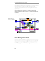
LabVIEW and Mathematica – Added Power
and Flexibility through a Synergistic Union
LabVIEW and Mathematica have two important features in common.
First, they are both high-level programming languages that allow
custom applications to be written efficiently. Second, programs written
with these languages can be run on a variety of operating
system/hardware configurations - specifically, under Windows or
Windows NT operating systems on computers that use Intel
microprocessors or their clones, under MacOS on the Apple Macintosh or
other computers based on Motorola 68K or PowerPC microprocessors, and
with UNIX on Sun, Hewlett-Packard, and other workstations.
LabVIEW and Mathematica both allow fast development of custom
portable applications, but each offers a completely different user
interaction paradigm and workflow. Interestingly, this is precisely
why these two applications can be viewed as extremely
complementary. Because their user interfaces are somewhat
antithetical, different aspects of a complex problem can be addressed
with the user interface that is most suitable to the given task. For
instance, in cases where interactive problem-solving or symbolic
manipulation is necessary, Mathematica’s textual command-line
interface is ideal. However, once a solution (or component of a larger
system) has been well-defined, LabVIEW’s RAD (rapid application
development) tools, built-in GUI elements and graphical programming
language provide a robust environment for high-efficiency deployment.
Combining these two diverse user interfaces interactively yields
completely new solution opportunities that are inaccessible using either
program alone.
2
Mathematica Link for LabVIEW
The Mathematica Front End
If you are a LabVIEW programmer and are new to Mathematica, it is
important to understand that the Mathematica user interface is
completely text-based. Mathematica programs are text files and are
entered by typing function-like command lines. The Mathematica front
end is an application—separate from the number-crunching kernel
—that is in charge of user interaction. The front end is where the
command lines are usually typed, but this is not merely a terminal
window. The purpose of the front end is to provide a user-friendly
working environment. The front end is used to generate documents called
“notebooks” in which you can place much more than the sequence of
command lines intended for the kernel. Notebooks are divided into cells
that are organized in a hierarchical structure. You can edit, comment
on, and organize your notebooks in whatever way that best supports the
requirements of your work. A notebook’s structure can be loosely
designed in any style that stimulates your creativity, or it can also be
very rigorously organized.
Thus, you can see that the Mathematica front end is similar to a word
processor, but it is a word processor connected to the kernel by
MathLink. (It should be noted that the Mathematica kernel can also be
accessed directly through a terminal window, or used with an array of
different front ends. One example is the Mathematica Link for
Microsoft Word, which enables Microsoft Word to act as an alternative
front end. )
LabVIEW Panels and Diagrams
In contrast with Mathematica, the LabVIEW interface is purely
graphical. LabVIEW programs, which are referred to as “Virtual
Instruments” (VIs), have two separate parts, the front panel and the
diagram. The front panel of a VI is usually the only part visible at runtime. It is composed of controls and indicators like those on the front
panel of a real scientific instrument. The diagram is the context where
the algorithm is actually implemented. As the name of this part of the
VI suggests, the diagram is not simply text, like the source files of
conventional programming languages. Rather, the diagram
graphically represents the flow of data to and from various terminals
(that is, diagram representatives of the front panel controls and
indicators), and external data sources. Data migrates from inputs to
outputs along a network of lines, or “wires” in LabVIEW terminology.
The nodes of the network are represented by operators or control
3
1 Introduction: What is Mathematica Link for LabVIEW?
structures that are found in any programming language. The major
difference between LabVIEW and conventional languages such as C or
Fortran is that the program step order of execution cannot be
anticipated from the diagram layout as it can be from the instruction
order of a source file. It is the availability of the input data from a
computation step that will initiate its execution. This data-flow model
makes LabVIEW algorithms parallel in nature even if the series of
computing steps must be computed sequentially by the CPU.
Furthermore, on platforms that support it, LabVIEW takes advantage
of the multithreading capabilities of the host operating system
(Windows, UNIX) to further overcome the limitations of sequential
computing.
Mathematica and LabVIEW - Diverse Computing
Capabilities
While the differences between the Mathematica and LabVIEW user
interaction models are profound, differences between these programs
are not restricted entirely to their user interfaces. Several differences
can also be uncovered in each program’s computing capabilities. Each
language has its specificity, which makes it more (or less) appropriate
for particular families of computing problems.
Mathematica is a general-purpose system for doing mathematics. It is a
rich programming language that allows a problem to be interactively
explored in many different ways. Its underlying architecture is based on
transformation rules and pattern matching, which in turn provides
powerful symbolic capabilities. Often Mathematica programs comprise
a large set of definitions or rules that are applied at evaluation time.
In most cases, the evaluation of a Mathematica program will last no
longer than just a few seconds. When an evaluation is running in the
kernel, you still can interact with the front end, but you cannot start
another evaluation until the one that is currently running is completed.
However, it is possible to connect your front end to several kernels
simultaneously. You can, for instance, assign the evaluation of cells
containing complex commands to a remote kernel running on a system
with a fast CPU while you keep your local kernel for less intensive
interactive evaluations. A Mathematica “session” is a series of inputs
and the corresponding outputs returned by a kernel.
Conversely, many LabVIEW programs are designed to run indefinitely
until you stop them. Due to the data-flow model, many tasks occur
simultaneously during execution. It is the programmer’s responsibility
4
Mathematica Link for LabVIEW
to prioritize tasks through time delays so that there is adequate
resources for higher priority operations. Moreover, since LabVIEW is
specifically oriented toward data acquisition and instrumentation, VIs
often interact with hardware located either inside the computer
(acquisition boards, for example) or at remote locations (connected via
one or more communication interfaces). Typically a LabVIEW program
is required to interact with one or more specialized devices at run-time.
Data acquisition and instrumentation applications often require various
instruments to be synchronized with one another, or with real-world
events such as triggers or user interaction. The pseudo-parallel structure
of LabVIEW diagrams and their timing functions, as well as their
ability to make use of dedicated hardware timers, allow VIs to
simultaneously manage all of these events.
Mathematica Link for LabVIEW - Practical
Implementations
In the opening paragraphs, we briefly discussed different ways of using
the Mathematica Link for LabVIEW package. Here, we will expand on
this further.
1. Run Mathematica as a subprocess of LabVIEW
Initially, it may be easiest to visualize implementations where
MathLink is used to run the Mathematica kernel as a subprocess of a
LabVIEW application. A particular computation step of your
application may be easier to access or to implement in Mathematica
than in LabVIEW. Perhaps you need to access one of Mathematica’s
sophisticated functions, or even the specialized, domain-specific
capabilities of dedicated third-party, add-on package. Either way,
the time spent building a communication link between LabVIEW and
Mathematica will be recovered by the time saved in using the
Mathematica programming language rather than LabVIEW for this
particular step.
2. Run a LabVIEW VI as a subprocess of Mathematica
Running the MathKernel as a subprocess of LabVIEW is often the
easiest place to begin. However, operating LabVIEW VIs or entire
LabVIEW applications from within the Mathematica notebook can
also be extremely valuable in the conduct of your R&D projects. If you
5
1 Introduction: What is Mathematica Link for LabVIEW?
are not yet used to interacting with your instruments from within
Mathematica notebooks, this use of Mathematica Link for LabVIEW
may sound less natural to you. Yet, when instruments are operated from
within a notebook, Mathematica becomes a kind of electronic
laboratory notebook offering a convenient way to automatically
document your experiments – simply save your notebook at the end of
each session to make a comprehensive record your entire session.
3. LabVIEW provides the GUI for your Mathematica
applications
Like LabVIEW, Mathematica provides a robust application
development environment. However, developing convincing, powerful
GUIs in Mathematica can be a challenging task. On the other hand,
LabVIEW’s diverse set of ready-made controls and indicators makes
GUI programming quick and easy. The Link gives you access to the best
of both worlds–the Mathematical intelligence and pattern-matching
prowess of Mathematica with the rapid GUI integration of LabVIEW.
4. Call Mathematica to generate publication-quality images
and reports with LabVIEW-acquired data
LabVIEW is an ideal development tool for data acquisition application
development. However, if you want to export your results in printed
form, your options are limited. LabVIEW’s bitmap export capabilities
and. html document generation is fine for on-screen review, but if you
want to produce hard-copy printouts the results can be disappointing. In
contrast, Mathematica offers a wide variety of document export options
– from Postscript and .PDF formats to .WMF (Windows Metafile
Format), and even AutoCAD .DXF files. Using the Link, a single
experiment or project can benefit from the powerful integrated DAQ
capabilities of LabVIEW while also enjoying the robust file export
capabilities of Mathematica.
5. Add sophisticated Mathematica data processing and
symbolic manipulation to LabVIEW applications
Admittedly, the Mathematical requirements of many programs are
well within the capabilities of LabVIEW. However, complex problems
can call for mathematically sophisticated solutions. Sometimes it is
much easier to approach a problem using symbolic representation –
particularly early in the project cycle when all aspects of the problem
6
Mathematica Link for LabVIEW
are not well understood or completely defined. In other cases, a solution
is well within LabVIEW’s capabilities, but in order to try several
different scenarios substantial wiring and rewiring is necessary. In the
exploratory phase, the flexibility of the text-based Mathematica
interface can provide several productivity advantages. The Link
provides interactive communication to Mathematica’s extensive
library of functions – any of which can be called upon interactively, and
without the need for rewiring. After the details of the solution have
been determined, you can continue to call Mathematica in a Link-based
hybrid application, or build a stand-alone LabVIEW-based solution.
6. Gain access to powerful Mathematica Add-on packages
There are several functions in the standard Mathematica packages
that have no LabVIEW counterparts. In addition, there are several
third-party add-on packages that may prove useful for advanced
instrumentation applications. Examples include Time Series, Signal
and System, Electrical Engineering, Experimental Data Analyst, and
Control System Professional, to name a few of the titles available. The
Link provides access to these powerful packages from within the
LabVIEW environment.
7. Take advantage of Mathematica’s powerful graphics
Mathematica has powerful and flexible graphical capabilities. You
may be interested in making direct use of high-level Mathematica
graphics functions such as Plot, Plot3D, ListPlot, and so forth. Use
these capabilities to plot an analytical function describing the
theoretical response of your devices. Or simply use these flexible
Mathematica commands to generate a graphical visualization of the
data you just collected. Mathematica also has a large set of graphical
primitives that enable you to build custom graphical functions. Thus,
you can use Mathematica Link for LabVIEW to display any kind of
graphical output that you can imagine.
8. Create Electronic Laboratory Notebooks
The GUI has become the de-facto standard in the computing world in
recent years. However in some circumstances, a text-based interface can
be preferable to a GUI. The Mathematica notebook interface becomes an
attractive alternative to the GUI for instruments and data acquisition
systems when LabVIEW applications and data acquisition hardware
7
1 Introduction: What is Mathematica Link for LabVIEW?
can be controlled using Mathematica Link for LabVIEW. One or a series
of Mathematica notebooks can function as a digital metaphor for
traditional, paper-based laboratory notebooks.
Traditionally, scientists involved in research would rigorously record
data in paper laboratory notebooks. In spite of the increased use of
digital technology in the laboratory, this traditional recording method
is still taught to graduate students. However, anyone who has done
experimental research knows the limitations of this approach – after a
few months it can be difficult to tell what precisely has been done. The
necessity of increasing research productivity and the requirements for
complying with regulations specific to quality control of laboratory
practice (Good Laboratory Practice, Good Manufacturing Practice) are
two reasons to find an alternative methodology. Moreover, given the
growing number of digital instruments in laboratories, and the growing
use of computer integrated data acquisition systems, physically pasting
data produced by these systems into paper notebooks is becoming an
increasingly anachronistic practice. Data can be incorporated into
documents such as word processing files, but no software has been
available specifically for the purpose of recording data in a notebooktype form.
Mathematica Link for LabVIEW could be used for this purpose. Given
that all the features of Mathematica notebooks are completely
described by kernel functions, it is possible to build Mathematica
programs that automatically generate documents. In this way
Mathematica can provide scientific computing and typesetting
functionality in a single environment. Mathematica has a greater
functionality than TeX, Fortran and other traditional scientific tools
because it provides hypertext features and an active link to the kernel
for evaluating Mathematica functions. Since the functions used to
describe notebooks are kernel functions the front-end application is not
needed. Thus, Mathematica programs could be developed to generate
custom reports from within LabVIEW applications without calling the
front end.
As previously mentioned, there are few commercial software packages
that can be used as electronic laboratory notebooks. The functionality of
the “new digital tools” is still being evaluated. Prototypes that can be
tested under real laboratory conditions will be required to prove the
concept. Currently Mathematica Link for LabVIEW does not have the
full functionality of an electronic laboratory notebook. Nonetheless, it
may be considered a first step in that direction. The package provides
the user with the ideal unified working environment – instruments and
8
Mathematica Link for LabVIEW
experiments can be controlled, and results can be reported
automatically.
9. Quickly build distributed LabVIEW applications
MathLink provides functions to exchange complex data in a
homogeneous way, independent of the computers used and the
underlying transfer protocol. Although LabVIEW provides other
“native” communication options (TCP VIs, DataSockets, VI Server, and
so forth), the MathLink libraries may also be used to distribute an
application among several computers. Such applications can be written
in a platform-independent way. The advantage is that you do not have
to master intricate protocols such as TCP or PPC to be able to write a
distributed application: MathLink functions take care of the details for
you. Once you are comfortable with MathLink programming techniques,
you will have the option of using the same high-level functions to
provide the communications mechanism for your distributed
applications.
10. Stand-Alone Mathematica Applications
Because Mathematica’s text-based interface is so flexible, users
unfamiliar with the syntax of the language may experience difficulties
when attempting to run applications in the standard Mathematica
front end. By embedding kernel evaluations into the LabVIEW
framework, you can build robust stand-alone GUI applications that
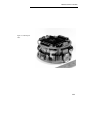
anyone can run. For example, the neural net used to run a Khepera robot
is easily computed in Mathematica. However, setting up the connection
weight matrix can be difficult due the abstract nature and large size of
the matrix. An attractive and convenient design is to build a VI where
the connection between neurons is graphically represented on the front
panel. The VI controls are used to set the weights of the neural net
connections. At run time, all the computation parameters (connection
weights and current state of the network) are passed to the
Mathematica kernel to compute the new state of the network. (For more
information and an actual example involving a Khepera robot, refer to
“Khepera.pdf”. This document and other support files are installed in
the LabVIEW/user.lib/MathLink/extra/Advanced/Khepera
directory.)
9
1 Introduction: What is Mathematica Link for LabVIEW?
10. A Powerful Synergistic Workflow
Mathematica Link for LabVIEW allows you to interact with your
instruments in an entirely new way. Using a combination of both
LabVIEW and Mathematica can create a more transparent user
experience – where the tools recede, and your attention is focused
directly on the problem at hand, rather than on overcoming the
limitations of the tools.
To expand on this further, consider a typical example. The
development of a measurement program often involves an initial stage
where you write a quick LabVIEW prototype to control and interact
with your instrument. This first prototype is rarely sufficient to produce
high-quality data: you may need to fine-tune your acquisition strategy,
redefine acquisition parameters, modify the sampling environment in
some way, reposition your sensors and so on, several times before you are
ready to collect useful data. Many trials yielding unusable results may
pass before the final data are recorded. At this stage of the process, you
need to forget the instrument as much as possible, and focus on the
research itself.
Now image how useful it would be if you could run a test and acquire a
sample with a single CallInstrument[] command. This single command
would return data directly into your Mathematica notebook, where you
could then interactively analyze the results in order to compute the
parameters for the next experiment. Imagine a workflow where you
simply call a new data set from your instruments on command, then
interactively process, analyze, plot, manipulate, plot again, and so
on...
Here is an example of a typical development loop for a hypothetical
experiment:
• Choose acquisition parameters, then make a data acquisition run
from within a Mathematica notebook.
• Analyze, process, and view the data returned by the instrument
interactively using advanced Mathematica functions.
• Use the results from your analysis to compute a new set of values for
the acquisition parameters.
• Return to the first step.
After the optimal experimental conditions are determined, you may
want to take additional steps, such as:
10
Mathematica Link for LabVIEW
• Saving your Mathematica notebook so the entire experiment can be
recreated and duplicated in the future.
• Developing a stand-alone LabVIEW VI with hard-wired
acquisition parameters for 100% repeatability.
• Extending the native LabVIEW functionality of your stand-alone VI
by calling advanced Mathematica data-processing, graphing, and
file export capabilities.
This hypothetical workflow exposes some of the opportunities offered
by the Link, but the details and requirements of your own applications
may introduce a completely different set. The key is to exploit the
relative strengths of the Mathematica and LabVIEW user interfaces,
and then realize the combined productivity benefits of both.
Programming and application examples illustrating all of the practical
implications noted above are included with the Mathematica Link for
LabVIEW package. (Programming examples are introduced in the
“Getting Started“ and “Programming” chapters later in this user
guide.)
Overview of Mathematica Link for
LabVIEW
This section provides a brief description of Mathematica Link for
LabVIEW’s functionality and multi-layered architecture.
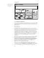
General Functionality
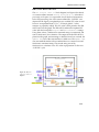
Mathematica Link for LabVIEW is a bi-directional communication
link. As implied in previous discussions, either application –
Mathematica or LabVIEW – can initiate a message, or be called as a
subprocess of the other. To clarify, LabVIEW can call the Mathematica
kernel as a subprocess, and/or Mathematica can call a LabVIEW VI as
a subprocess.
Calling Mathematica from LabVIEW
Using the Mathematica kernel from within LabVIEW is somewhat
similar to using formula nodes in LabVIEW application diagrams.
However, Mathematica Link for LabVIEW offers one important
advantage: whereas a formula node resides on a VI diagram, and the
VI must be stopped and restarted to change the formula, a
11
1 Introduction: What is Mathematica Link for LabVIEW?
Mathematica string can be specified in a standard string control on a VI
front panel, or generated programmatically. Changes made to the
control string at runtime can be passed immediately to Mathematica for
evaluation, so new formulae and functions can be attempted
interactively, without stopping the VI.
Mathematica Link for LabVIEW provides you with a small set of
high-level VIs that can be thought of as Mathematica nodes. For
example, one of the bundled VIs evaluates Mathematica expressions
using properly formatted strings as arguments, and injects the returned
results into the VI diagram.
Other VIs are dedicated to graphical output. Integration of these VIs
into your LabVIEW application is consistent with the LabVIEW
interface, even for graphics, since Mathematica images are returned
and displayed as intensity graphs. When the kernel and LabVIEW are
running on the same computer the usual Mathematica evaluations
execute quickly. However, functions that return graphics take longer
than typical Mathematica evaluations because an intermediate
PostScript interpretation step is required.
Calling LabVIEW VIs from a Mathematica Notebook
VIs can also be opened and run interactively from the Mathematica
front end. The custom VIClient.m package (included in the Link
package) interfaces with the specialized MathLink VI Server.vi
to provide a flexible, yet easy-to-use command interface for launching,
running, and disposing of VIs.
The command syntax for controlling VIs is consistent with LabVIEW
terminology, past and present. LabVIEW veterans may prefer to use
victl.llb terminology:
PreloadInstrument[]
CallInstrument[]
ReleaseInstrument[]
and so forth.
People new to LabVIEW and users comfortable with the newer VI
Server terminology will likely prefer a command structure consistent
with VI Server conventions:
OpenVIRef[]
RunVI[] (or CallByReference[])
12
Mathematica Link for LabVIEW
CloseVIRef[]
and so on.
(More information about the VIClient.m package, the specialized
MathLink VI Server.vi, and Mathematica’s VI Server commandline syntax is presented later in this section and at various other places
throughout this user guide.)
Structure of the Link
The low-level component that provides the communication link
between the Mathematica kernel and the outside world is Wolfram’s
own MathLink. MathLink is a library of C functions that manage
program-to-program communication. The MathLink protocol is
responsible for all communication with the kernel, including
communication with the standard Mathematica front end. This
protocol can also be used to establish a connection between the kernel
and an external MathLink-compatible program. (Interested parties are
directed the Mathematica documentation for more information about
MathLink.)
Mathematica Link for LabVIEW leverages the MathLink code base.
The MathLink functions are made accessible to LabVIEW through a
Code Interface Node. Several VIs are included to implement the most
commonly used MathLink functions, but all of these VIs call a common
CIN VI. Inside this single CIN VI the MathLink C functions are
actually called. This CIN VI also includes a function to read files
generated by the PostScript interpreter MLPost. (Refer to “Software
Architecture” on page 62, for a more detailed description.)
High-Level Functions
The following VIs provide direct access to the most common Link
functions, and are designed for users with only a minimal familiarity
with MathLink. They provide ready-made solutions for a variety
of standard applications.
MathLink VI Server.vi
This VI is a bridge between MathLink and the various VIs of the
LabVIEW VI control library. A number of Mathematica functions have
been designed that are strict Mathematica equivalents of these VIs.
Thus you can use functions such as OpenVIRef, OpenPanel, RunVI, and
13
1 Introduction: What is Mathematica Link for LabVIEW?
others to operate your LabVIEW applications. These applications can
run either on the same computer or on two different computers linked
over a network.
Kernel Evaluation.vi
This VI passes a string of Mathematica commands (in the usual
Mathematica syntax) to the kernel for evaluation, and returns the
results to LabVIEW. You need to specify the expected data type for the
result from among a finite number of data types: Boolean, Integers,
Real, Complex, Strings, and lists and matrices of all these types. The
result of the evaluation is returned on the indicated connector of the VI.
Kernel Evaluation.vi has high-level functions to manage all
aspects of Mathematica sessions, such as printed messages, error
messages, etc. You can use it as a general-purpose interface to
Mathematica functions within the diagrams of your LabVIEW
applications.
Mathematica Graphics Generators
Four VIs are provided to make Mathematica graphical functions
available to LabVIEW. Generic ListPlot.vi displays a graphical
representation of sets of data. Generic Plot.vi is used to visualize,
from within LabVIEW, graphics returned by Mathematica commands.
Display Bitmap.vi is similar in function to Generic Plot.vi, but
uses Mathematica graphic functions to generate a .BMP (rather than a
PICT) file. Generate Graphic File.vi illustrates how images
generated in Mathematica can be exported to one of several different
image file formats.
Development Tools
A number of VIs can help you build your own MathLink applications.
They combine the action of several MathLink functions in ways
frequently encountered when developing MathLink applications.
Data Transfer VIs
Thirty VIs are provided to transfer the most commonly used data
structures (mainly lists and matrices of all kinds). They are documented
and their source code is accessible, so they can be a basis for building
new VIs to transfer other data structures that have not yet been
implemented.
14
Mathematica Link for LabVIEW
Error Handling VIs
Mathematica Link for LabVIEW follows the LabVIEW error cluster
scheme for managing MathLink errors. All the VIs have “Error in” and
“Error out” clusters. A MathLink Error Manager.vi, based on
General Error Handler.vi, is provided to identify MathLink
errors and take the appropriate corrective action when possible.
MathLink VIs
Forty-three of the most commonly used MathLink functions are
implemented in Mathematica Link for LabVIEW.
Development Environment
A number of examples are provided to illustrate how the MathLink VIs
can be used in various combinations in LabVIEW applications. Some of
the examples are based on the standard VIs contained in the LabVIEW
distribution. Others—such as the PID Control Demo and the
Mathematica Shape Explorer—are entirely new VIs, developed
for the package using Link components as subVIs. Some of the standard
VI library examples are slightly modified to take advantage of
MathLink functions more efficiently. Comments, guidelines, and
recommendations are also provided in the VIs to accelerate the
development of your own MathLink applications.
Some real applications to control the Khepera mobile robot are also
included. Although they cannot be run without the robot, they
illustrate the possibility of developing robust real-time applications
with Mathematica Link for LabVIEW.
For basic work, you might be satisfied to use the higher-level VIs of
Mathematica Link for LabVIEW. However, as you continue to work
with Mathematica Link for LabVIEW, you will soon realize that it is
truly an open development environment that allows you to make
creative use of the respective strengths of Mathematica and LabVIEW.
Also, depending on the application, you may wish to have an interface
that is more oriented toward either Mathematica or LabVIEW. Once
the interface has been chosen, you are still completely free to
implement each step of your algorithm in the most appropriate
language. In successive revisions of your application, the language that
a particular step is written with may even change. For example, you
may first use Mathematica in a phase where you want to prove a
concept with minimal development cost. Later, after the algorithm has
15
1 Introduction: What is Mathematica Link for LabVIEW?
been validated, it can be valuable to rewrite the procedure in LabVIEW
for speed and integration.
Thus, Mathematica Link for LabVIEW provides a new development
framework that neither LabVIEW nor Mathematica can claim on its
own. The portability of each of the components of this association
ensures that applications written with Mathematica Link for
LabVIEW will also be portable.
16
2 Installation
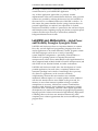
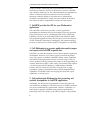
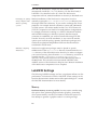
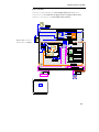
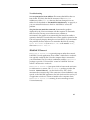
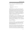
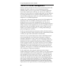
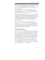
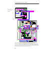
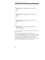
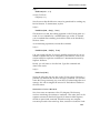
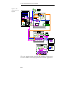
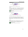
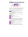
Mathematica Link for LabVIEW uses an innovative VI-based installer.
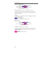
When the installation CD is inserted, Install.vi automatically
launches LabVIEW on the target system and begins the installation
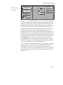
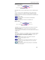
process (see Figure 1). The VI-based installer is an ideal choice for
LabVIEW toolkit installation offering several distinct advantages
over conventional software installers. Specifically, it can quickly and
easily locate the target LabVIEW directory on your system and initiate
VI Server functions to initialize VI parameters during the installation
process.
In most cases, link components are automatically configured to run
properly without any user intervention. While you also have the
option of installing all Mathematica Link for LabVIEW components
manually (as discussed later in this chapter), the VI-based installer
offers a complete, automated solution for the majority of installations.
Figure 1. Install.vi
VI-based installer
splash screen.
2 Installation
The default installation assumes Mathematica and LabVIEW are both
installed on a single target PC. The target PC drive is first scanned for
installed copies of LabVIEW and Mathematica. After the user confirms
the target path locations, the toolkit files are installed in the
appropriate places within the LabVIEW and Mathematica file
systems. The default installation is recommended whenever possible to
ensure the full functionality of all Mathematica Link for LabVIEW
components. If Mathematica and LabVIEW will run on different
systems, and your network topology does not permit you to locate the
Mathematica directory from inside LabVIEW using a standard file
browser, you may need to install the Mathematica components
manually. (Manual installation and other non-standard installation
requirements are discussed in “Non-standard Installation Options”
beginning on page 21.)
Standard Installation Procedures
This section describes the standard installation process in more detail.
Since Install.vi was constructed using LabVIEW itself, the
installation process is identical for both MacOS and Windows
platforms.
System Requirements
This distribution of Mathematica Link for LabVIEW is designed for
LabVIEW 6.0 or higher* and Mathematica 4.1 or higher*.
Mathematica and LabVIEW should be installed on the same PC, or one
of the applications should be installed on a second computer accessible
to the first over a TCP/IP network. Any system (or combination of
systems) that can run LabVIEW and Mathematica effectively should
be appropriate for Mathematica Link for LabVIEW. If you are unsure
about the capabilities of your system, please refer to the LabVIEW and
Mathematica documentation for detailed system requirements.
*IMPORTANT NOTE: Neither Mathematica nor LabVIEW is part of
the Mathematica Link for LabVIEW package: each must be purchased
separately. For information about support for previous version of
Mathematica and/or LabVIEW, contact BetterVIEW directly.
18
Mathematica Link for LabVIEW
Windows 95/98/ME/NT/2000/XP
The components in this installation are compatible with Windows 95,
98, ME, NT (Version 3.51 or later), 2000, and XP. Mathematica Link for
LabVIEW cannot run under Windows 3.1.
MacOS
The MacOS version of Mathematica Link for LabVIEW will run on
MacOS 7.6, 8.x, and 9.x . Version 8.5 or higher is recommended. (MacOS
X is not supported at this time, and the package has not been verified
for use in the MacOSX “Classic” environment. A native OSX version is
under consideration. Contact BetterVIEW directly if you are interested
in native MacOSX support.)
Disk Space Requirements
The full installation requires approximately 20 MB of disk space. If you
plan to use Mathematica on a remote computer, you may also need to
install networking software.
Installing the CD-ROM version
1. Mathematica Link for LabVIEW is available in two formats: a CDROM distribution, and an electronic distribution. (For electronic
distribution installation instructions, see page 20.) To install the
CD-ROM version, begin by inserting the CD into the appropriate
place your on your PC.
2. The VI-based installer, Install.vi is configured to auto-run when
the CD is inserted. If LabVIEW is running when the CD is inserted,
the VI will load immediately. If LabVIEW is not running, it will
launch before Install.vi loads. If the CD auto-run capability
has been disabled on your PC, simply open the CD and double-click
on the Install.vi icon. Alternatively, you can manually open the
VI from inside the LabVIEW editor.
3. Once running, Install.vi walks you through the necessary
installation steps. Select the items to install using the large yellow
checkboxes provided. If both LabVIEW and Mathematica will run
on the same system, be sure to check both items: “Install LabVIEW
Components” and “Install Mathematica Components”.
4. After selecting the components to install, you will be asked to verify
the installation paths. Install.vi uses more than one platformspecific search strategy to determine the most likely target paths.
19
2 Installation
However, an inappropriate path is sometimes selected if several
instances of Mathematica or LabVIEW are installed on the target
PC, or if Mathematica and LabVIEW are installed on different PCs,
drives, or drive partitions. Be sure to verify, and if necessary,
specify alternate paths before initiating the installation step.
5. Follow the instructions provided by the installer and review the
online installation notes for additional information and last minute
changes.
6. A Mass Compile option has been added to the exit page of the VIbased installer. Click the Mass Compile button if you would like to
update the main toolkit components for the version of LabVIEW you
are running. (Note: to minimize the time required, some secondary
Link components are not updated by the Mass Compile function.)
7. Register your copy of Mathematica Link for LabVIEW by selecting
the On-line Registration option on the Exit page of Install.vi, or
by filling in the Application Library Registration Form accessed
from the LabVIEW item in the Add-ons section of the Mathematica
Help Browser (see next subsection).
8. To finish the installation, quit and restart LabVIEW. When
LabVIEW restarts, you will have direct access to the Link
components through the Function and Control palettes. Also, you will
discover that new MathLink items have been inserted in the
LabVIEW Help and Tools menus.
REBUILDING THE MATHEMATICA HELP INDEX
Before you can use the freshly installed Mathematica documentation
and Hands-on exercises, you will also need to rebuild the
Mathematica Help Index. Launch Mathematica then simply select
Rebuild Help Index in the Help menu.
Installing the Electronic Distribution
If you have purchased the electronic distribution of Mathematica Link
for LabVIEW, the first two installation steps are slightly different.
Begin by expanding the compressed .zip (Windows) or .hqx (MacOS)
archive. Open the resulting installer folder, and double-click on
Install.vi. Proceed with the rest of the installation beginning with
step 3 from the CD-ROM installation instructions (listed previously).
20
Mathematica Link for LabVIEW
Uninstalling Mathematica Link for LabVIEW
No dedicated uninstaller application has been included with this
package. However, Mathematica Link for LabVIEW components can be
uninstalled manually by removing following directories and all of the
items they contain:
LabVIEW/user.lib/MathLink
LabVIEW/project/MathLink
LabVIEW/menus/MathLink
LabVIEW/help/ML_Help.vi
LabVIEW/help/ML_UserGuide.pdf
Mathematica/AddOns/Applications/LabVIEW
More detailed information about the organization and file structure can
be found in the section entitled “Organization of Mathematica Link for
LabVIEW” on page 23.
Non-standard Installation Options
Most configurations can be accommodated using the VI-based installer,
and whenever possible, this is the preferred installation method. The
VI-based installer uses VI Server functions and Mathematica path
information to automatically configure Link components. Still, some
users may have specific requirements that are not specifically
supported by the installer. The most common variations are discussed
next.
LabVIEW and Mathematica Running on Different PCs
Some users may prefer to run Mathematica and LabVIEW on different
PCs to distribute the processing load, or simply because the LabVIEW
and Mathematica licenses are assigned to different PCs. If LabVIEW is
installed on both PCs, simply run the installer on each PC and install
only the files corresponding to the resident application. More often,
LabVIEW will be installed on only one of the PCs. In this case, you may
be able to run the installer on one PC and manually browse the second
PC’s drive to locate the target Mathematica directory across the
network. If you want to install only the LabVIEW components or only
the Mathematica components in a particular session, simply set the
large checkboxes accordingly on the Installation Selection page
21
2 Installation
of the installer VI. If Mathematica and LabVIEW components are
installed in different sessions, you will be required to manually
configure the Math Kernel path information in Launch Kernel.vi.
This relatively simple procedure is discussed on page 22.
Installing Mathematica Link for LabVIEW components in
non-standard places.
IMPORTANT NOTE: While it is possible to use Install.vi to install
the various components of the Mathematica Link for LabVIEW
package in any location you choose, this practice is not recommended.
On-line documentation, Tool menu functionality, and direct access to
Link elements from within Mathematica and LabVIEW are only
available when the components are installed in the intended locations.
Auto-Installation to Non-standard Locations
Manually locate the preferred destinations using the file browser
buttons on the installer's main installation page. Then, after
acknowledging the warning dialogs, proceed with the installation.
Manual Installation
The VI-based installer has been included to automate the installation
process. However, you also have the option of manually copying the
files from the CD into any location on your drive. This option is
convenient if you only want to install or re-install a specific component.
Manual installation also provides a useful workaround if you
experience a problem with the VI-based installer. If you are familiar
with the organization of the LabVIEW and Mathematica file
structures, the destinations will be somewhat self-explanatory. If you
are new to either LabVIEW or Mathematica, refer to “Organization of
Mathematica Link for LabVIEW” on page 23 for additional background
information.
Configuring the MathKernel Path in Launch
Kernel.vi
One of the duties performed by the VI-based installer is to set the
default value of the MathKernel Path parameter in Launch
Kernel.vi This enables LabVIEW to automatically negotiate a
MathLink connection without user intervention. If you install the Link
22
Mathematica Link for LabVIEW
components manually or using separate installer sessions, the VI-based
installer cannot take care of this task for you.
If you have performed a manual or non-standard installation, you must
set the default MathKernel path manually. First locate the
MathKernel executable in the Mathematica file hierarchy, and make
a note of the full path. (On the Windows platform, MathKernel.exe is
typically found in the top level of the Mathematica file system.
MacOS users can usually find it inside the Mathematica
Files:Executables:PowerMac folder.)
Next, launch LabVIEW and open Launch Kernel.vi. This VI can be
found in MLStart.llb, located in the LabVIEW/user.lib/MathLink
directory. Enter the full MathKernel path from the previous step into
the MathKernel Path control on the front panel. Set this value as the
default by right-clicking on the modified path control (option-clicking
on the Mac) and selecting the Set as Default option. Save the VI to
finalize the change and close the panel. Your Mathematica Link for
LabVIEW VIs should now be configured to automatically negotiate a
MathLink connection.
Organization of Mathematica Link for
LabVIEW
The Mathematica Link for LabVIEW installation process creates new
directories in both the Mathematica file system and in the LabVIEW
file system. Installed Link components interact with the MathLink
libraries installed in your system directory by the Mathematica
installer. The Mathematica Link for LabVIEW file system is described
in detail in this section.
The MathLink Subdirectory of the User.lib Directory
The majority of the Mathematica Link for LabVIEW distribution files
are placed in the MathLink subdirectory of the user.lib folder,
which is located inside the main LabVIEW directory. The MathLink
directory contains the VI libraries MLStart.llb and Tutorial.llb
and four subdirectories named dev, extra, LabVIEW, and MLPost.
MLStart.llb provides a collection of standard high-level VIs that
can be used as limited stand-alone applications, or as the basis for
further development. These VIs are described in the section “The
MLStart.llb Library” on page 29.
23
2 Installation
Tutorial.llb contains the example VIs introduced in the “Getting
Started” and “Programming” chapters later in this User Guide.
The dev directory contains five VI libraries: MLComm.llb,
MLGets.llb, MLFast.llb, MLPuts.llb, and MLUtil.llb.
Collectively, these libraries contain the VIs necessary to implement
the low-level MathLink functions. In MLComm.llb you will find all
MathLink functions dealing with communication management of the
link. MLGets.llb and MLPuts.llb, respectively, contain MathLink
functions for “getting” and “putting” data to and from the link.
MLFast.llb contains a collection of higher-level functions used to
transfer common data structures. Finally, MLUtil.llb provides VIs
that are not part of MathLink but that are used either as subVIs of the
VIs in the previous libraries, or to manage general aspects of MathLink
sessions in LabVIEW applications.
The extra subdirectory contains additional application examples and
advanced topics. Here, you will find the Mathematica Shape
Explorer.vi, a MathLink Simulation and PID Control demo,
additional graphics examples, and an advanced application tutorial.
The extra folder also contains several VIs and supporting
documentation for MathLink operation and control of a Khepera robot.
The items in the extra folder are useful, both as quick demonstrations
of the capabilities of Mathematica Link for LabVIEW, and as an
introduction to how various components can be used in the development
of larger projects.
The MLPost directory contains the MLPost application, a PostScript
interpreter used for rendering Mathematica graphics in LabVIEW (see
the section “Graphics Rendering” on page 92).
The LabVIEW subdirectory of the MathLink directory contains
Mathematica material and additional advanced programming
examples. During the standard installation, a copy of this directory is
also placed in the Mathematica file system. The contents of the
LabVIEW subdirectory is described in more detail in the section “The
LabVIEW Subdirectory of the Mathematica Applications Directory”
on page 25.
Use the readme.vi
utility to browse the
content of Mathematica
Link for LabVIEW.
Each subdirectory installed in the user.lib folder also includes a
dir.mnu where icons and structures of floating palettes are saved. (If
you are not familiar with this LabVIEW feature, consult the LabVIEW
documentation for more specific information). In addition, short
descriptions of every library or VI are provided as .txt files that can
24
Mathematica Link for LabVIEW
be read by the readme.vi utility found in the examples directory of
the standard LabVIEW distribution.
Other LabVIEW Directories Affected by Mathematica Link
for LabVIEW Installation
The installation process also affects other directories of the LabVIEW
file system:
On line version of
the User's Guide.
A complete online version of this manual - the Mathematica Link for
LabVIEW User Guide – is installed in the help directory. This
document can be accessed through the MathLink item in the
LabVIEW Help menu .
Run the top-level VIs
and examples from the
LabVIEW Tools menu.
A MathLink subdirectory is also created in the project directory of
the LabVIEW file system. This allows you to launch the main VIs from
this distribution directly using the MathLink item in LabVIEW’s
Tools menu .
Use the MathLink
palettes to enhance
your productivity.
A MathLink sub directory is also added to the LabVIEW menu
directory. The file in this folder adds Mathematica-oriented palette
sets to the Control and Function palettes. You can access the custom sets
by selecting the MathLink Palette Set in the Control or Functions
palette Options dialog. (For more information about setting and
selecting custom palette sets, refer to the LabVIEW documentation.)
The LabVIEW Subdirectory of the Mathematica
Applications Directory
If you intend to use Mathematica Link for LabVIEW to control
LabVIEW applications from within Mathematica, it is necessary to
configure your Mathematica installation. The configuration procedure
is explained in this section.
If the VI-based installer is used to perform a standard installation (as
outlined earlier in this chapter), the Mathematica configuration is
completed automatically. A second complete copy of the
user.lib/MathLink/LabVIEW directory is installed in the
Applications directory of the Mathematica file system.
When running Mathematica and LabVIEW on different systems, the
LabVIEW directory containing the VIClient.m file is the only
component of the distribution that must be placed on the computer
running Mathematica. If LabVIEW is also installed on the computer
25
2 Installation
that will run Mathematica, simply use the installer VI to
automatically install the LabVIEW directory. On the other hand, if
LabVIEW is not installed on the PC where the Mathematica
components will run, manual installation is necessary as described next.
Exchanging the package
among computers under
different operating
systems.
Manual installation of the Mathematica components involves
manually copying the user.lib/MathLink/LabVIEW directory into
the target Mathematica directory. If you need to exchange files across
platforms—for example, between a Windows system and a Macintosh
or UNIX system— the easiest method is often via a TCP/IP network.
(TCP/IP is required to use MathLink in multi-platform configurations–
for example, Mathematica running on a UNIX or Macintosh machine
and LabVIEW running on a Windows system). After the network
connection is established, you can then transfer files using FTP (File
Transfer Protocol), an email attachment, or any native file transfer
options your network topology permits. Mathematica packages and
notebooks are platform-independent ASCII text files that must be
transferred in ASCII mode.
Manually configuring
Mathematica.
Mathematica application packages must be placed in specific
subdirectories of the Applications directory located inside the Addons directory of the main Mathematica directory. In order to configure
your system correctly, place the entire LabVIEW directory, and all of its
contents, into the .../Mathematica/AddOns/Applications
directory. Next, launch Mathematica and select Rebuild Help Index in
the Help menu. This will add a new item named LabVIEW in the
AddOns section of the Mathematica help browser. Manual installation
of the Mathematica components is now complete.
LabVIEW Settings
The following LabVIEW settings can have a significant influence on the
performance of Mathematica Link for LabVIEW. (These settings can be
found in the Performance & Disk section of the Options dialog box – consult
the LabVIEW documentation for more details.)
Memory
Deallocate memory as soon as possible: You may want to consider using
this option when generating high-resolution graphics, particularly
when system memory resources are limited. Activate this option if a
first attempt to generate a graphic results in a warning message
26
Mathematica Link for LabVIEW
stating that the available memory is low and more memory cannot be
allocated to LabVIEW.
Compact memory during execution (Macintosh only): This option can
also help in coping with memory-shortage problems, especially with
graphics-intensive applications.
Cooperation Level (Macintosh Only)
In most typical Mathematica Link for LabVIEW configurations, the
Mathematica kernel and your LabVIEW application will share the
same CPU. If performance is an issue, it can be critically important to
adjust the time yielded by each application to the other. If you need
good performance on the LabVIEW side, and only require short
evaluation periods for the Mathematica kernel, you should set the
cooperation level to “low".
In some cases you may need to interact with the two applications at the
same time. For instance, if you want to control a VI from within a
Mathematica notebook, you may need to switch back and forth
frequently between the Mathematica front end and LabVIEW. In this
situation, setting the cooperation level to “high” may improve the
response of your application significantly. When the cooperation level
is set to “low”, switching from LabVIEW to another application occurs
much more slowly. Thus, setting the cooperation to a high level may be
advisable even though it can impact the execution speed of your
LabVIEWapplication.
27
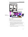
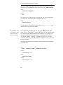
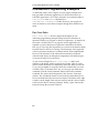
3 Getting Started
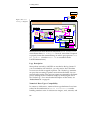
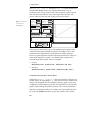
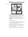
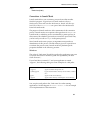
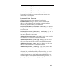
Immediate Gratification
If you are interested in immediate, hands-on interaction with
Mathematica Link for LabVIEW, there are a couple of options
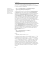
available to you. If you would first like to see the Mathematica kernel
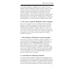
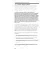
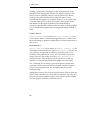
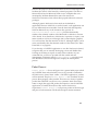
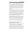
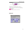
operating as a sub-process of LabVIEW, experiment with the
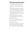
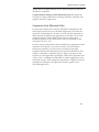
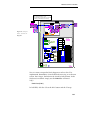
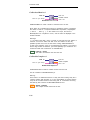
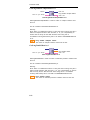
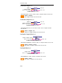
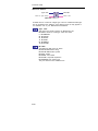
Mathematica Shape Explorer.vi or the PID Control Demo.
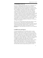
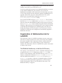
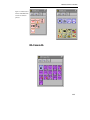
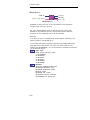
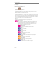
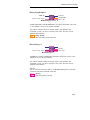
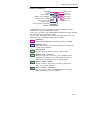
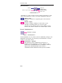
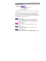
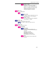
Both of the demos can be accessed via the MathLink -> Extras menu of the
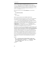
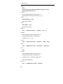
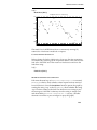
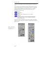
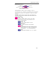
LabVIEW Tools menu (see Figure 2).
Figure 2. Accesssing
MathLink items in the
LabVIEW Tools menu.
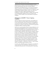
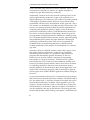
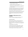
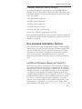
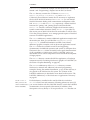
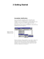
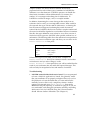
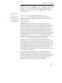
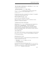
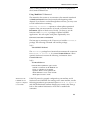
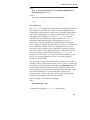
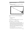
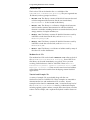
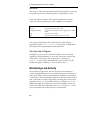
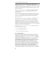
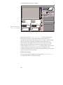
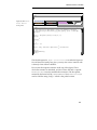
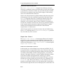
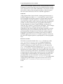
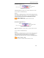
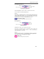
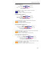
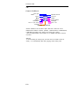
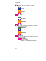
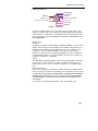
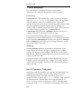
Readers interested in calling LabVIEW VIs from inside a Mathematica
notebook are directed to the hands-on tutorials installed with the
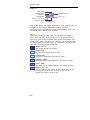
Mathematica files. After Mathematica Link for LabVIEW has been
installed, you can access the tutorials from the AddOns section of the
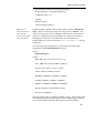
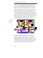
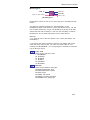
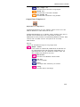
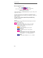
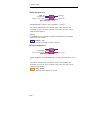
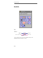
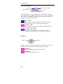
Mathematica Help Browser (see Figure 3).
3 Getting Started
Figure 3. Accesssing the
Hands-on Tutorials from
the Mathematica Help
Browser.
Alternatively, you can find the raw tutorial notebook files –
HandsOn_Part1.nb, HandsOn_Part2.nb, and HandsOn_Part3.nb, in
the following Mathematica subdirectory:
…\AddOns\Applications\LabVIEW\Documentation\English\
(Note: This material can also be found in the LabVIEW file system,
inside the user.lib\MathLink\LabVIEW\Documentation
subdirectory.)
If you have any difficulty locating and running these items, review the
previous Installation chapter to ensure that the Mathematica Link for
LabVIEW components have been installed and configured properly.
These introductory materials are intended to get you working with the
Link components immediately, but provide very little background
information. Additional insight into Link components and operations is
provided in the text that follows.
The MLStart.llb Library
In this section you will learn to use the four top-level VIs of
MLStart.llb:
30
•
Kernel Evalution.vi
•
Generic ListPlot.vi
•
Generic Plot.vi
Mathematica Link for LabVIEW
•
MathLink VI Server.vi
Understanding these VIs will give you a glimpse into the fundamental
capabilities of Mathematica Link for LabVIEW.
Kernel Evalution.vi can be used within LabVIEW diagrams to
request a computation step from the Mathematica kernel.
Generic ListPlot.vi provides the Mathematica data
visualization tools for LabVIEW data sets from within LabVIEW
applications.
Generic Plot.vi can be used to plot, from within LabVIEW,
analytical functions specified in Mathematica syntax.
MathLink VI Server.vi is the tool that controls LabVIEW VIs and
applications from within Mathematica notebooks.
Next, we will look at each of these VIs individually.
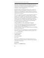
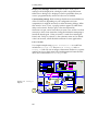
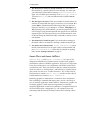
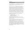
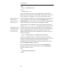
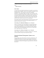
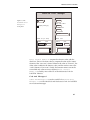
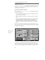
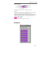
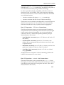
Kernel Evaluation.vi
Kernel Evalution.vi allows you to send computation requests to
Mathematica’s kernel as strings. You can type Mathematica commands
in this VI’s “Command” box just as you would from within a
Mathematica notebook. However, it is also necessary to specify the
data type that you expect as the result of the computation.
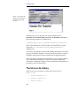
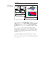
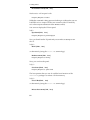
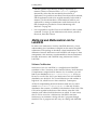
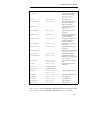
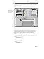
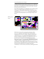
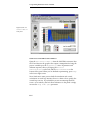
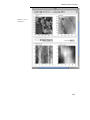
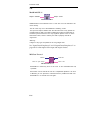
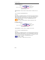
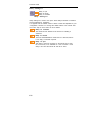
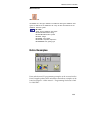
The result of the computation is sent to the appropriate element of one
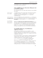
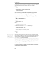
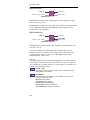
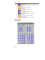
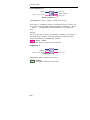
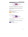
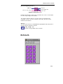
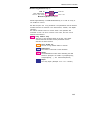
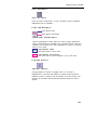
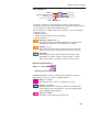
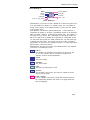
of the three clusters positioned on the right side of the front panel. In
Figure 4 only the “Basic data” cluster is displayed. Two other clusters—
“1D Arrays” and “2D Arrays”—which are used to collect lists and
matrices of data, are not visible in the operational mode depicted in
the figure.
31
3 Getting Started
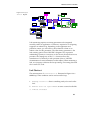
Figure 4. The Kernel
Evaluation.vi
front panel.
Kernel evaluation
Command
2+2
Expected type
Integer
Syntax log
1
0
New session
True
Abort previous evaluation
False
Display error messages
True
Custom timing settings
False
0
Basic data
Packet log
Boolean
0
False
LASTUSERPKT
Link in
0
error in (no error)
status
no error
code
0
source
Link out
0
status
no error
0
Message log
Real
0
error out
Integer
0,0000E+0
code
0
source
Complex
Menu log
0
Menu code
0,0000 +0,0000 i
String
0
Prompt string
Use of Kernel Evaluation.vi
This VI can be used either as a main application, or as a subVI in larger
applications. Some advanced settings to optimize its performance are
discussed later.
BASIC OPERATION
The default values of the controls are set so that you can run the VI
immediately. If you worked through the hands-on exercises introduced
at the beginning of this chapter, you have already used this VI to
compute the result of 2+2. If you skipped over the tutorial exercises,
type 2+2 into the “Command” box and run this VI now to verify your
installation of Mathematica Link for LabVIEW. (If you experience
difficulties, refer to the Troubleshooting notes at the end of this
discussion.)
The initial evaluation will take slightly longer than subsequent runs
because the Mathematica kernel must be launched on the first run.
However, once the evaluation is completed, the result is displayed in
the “Basic data” cluster on the right. In this case it appears under
“Integer”, since the “Expected type” was set to “Integer”, as is
appropriate for the expected result of 2+2.
Next, you can try a simple operation that returns a string. In the
“Command” box type "MathLink for "<>"LabVIEW". Select “String”
in the “Expected type” list and run the VI again. The expected
32
Mathematica Link for LabVIEW
concatenated string appears in the “String” box in the “Basic data”
cluster.
You can also perform a computation involving a more complex data
type. For example, enter Range[10]^2 with “1D Integers” selected. The
“Basic data” cluster disappears and the “1D Arrays” cluster becomes
visible. This feature limits the number of objects that are present at any
one time on the front panel.
CUSTOM SETTINGS
New session. A sequence of requests issued by Kernel Evaluation.vi
constitutes a Mathematica session. Since definitions are retained
throughout the session, it is sometimes helpful to restart the kernel as a
means of removing conflicting definitions, or simply as a way to free
memory. “New session” is the way to restart the kernel. Its default
value is “True”, so that a new session is automatically started when the
VI is run for the first time. But, after completion, “New session” is reset
to “False” so that subsequent evaluations will be performed within the
same session. You can, however, manually or programmatically set this
control to “True” in order to quit and restart the kernel.
Abort previous evaluation. This control is used to abort a running
evaluation. Kernel Evaluation.vi—and any other VI sending
computations to the Mathematica kernel for that matter—should not be
permitted to lock out the user with an infinite or very long evaluation.
There is a time out control implemented: if the time out is exceeded,
then no result is returned. This means that the indicator corresponding
to the selected data type will not be updated and this may be easily
overlooked. Another way to see that no result was returned is to
determine whether a new packet was added to the “Packet log”
indicator (see “Logs Description” on page 36, for details).
When such a situation occurs, it is useful to be able to abort the running
calculation before sending the next one. Set “Abort previous evaluation”
to “True” in this case. An instruction to abort the computation will be
sent to the kernel before the next command. Make sure that there is an
evaluation running before sending an abort command, otherwise the
kernel may quit (see “Troubleshooting” on page 37). As an example of
this feature, send the following command to the kernel: While[True].
Nothing will be returned. Afterwards send Names["System`*"] with
the “Abort” button turned on and with “1D Strings” selected as the
expected data type.
33
3 Getting Started
Display error messages. When this control is set to “True”, error
messages will be displayed in a dialog box with a single OK button.
Otherwise no dialog box is displayed, which is preferable when you
want to programmatically control how the error is handled.
Custom timing settings. Built-in timings should ensure smooth behavior
of this VI. However, depending on your configuration and your
computations, it might be necessary to refine the timing settings. When
this control is set to “True”, a pop-up window appears in which three
delays can be tuned. “Delay to quit” is the time required by
Mathematica to quit, and is used when you start a new session. It is then
necessary to allow some time after closing the link before attempting to
launch the kernel again. “Delay to launch” is used when starting the
kernel, and “Delay to evaluate” is the evaluation time out. Its default
value is 60 seconds, which should be sufficient for most applications.
USE AS A SUBVI
Two simple examples using Kernel Evaluation.vi as a subVI are
included in Tutorial.llb. They are Good PrimeQ.vi and Bad
PrimeQ.vi. Both VIs test an integer to determine whether it is a prime
number, but (as per their names) one implementation is better than the
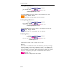
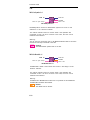
other one. Let us examine Bad PrimeQ.vi first.
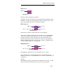
Test results
0
Test Progress
Data set size
Graph
Progress
Maximum
PrimeQ[
]
Boolean
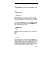
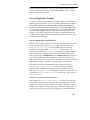
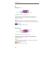
Figure 5. Bad PrimeQ.vi
diagram.
Range
0
Test Progress
ms
Elapsed Time
34
Mathematica Link for LabVIEW
Open the diagram of Bad PrimeQ.vi. Before running the VI, make
sure that your kernel is not still connected to Kernel Evaluation.vi.
In order to close the connection, run Close All Links.vi (this VI can
be found in MLUtil.llb, or can be accessed via the LabVIEW Tools
menu under MathLink -> Utilities -> Close All Links...).
In Bad PrimeQ.vi, each number is tested separately with the
comparatively trivial Mathematica command, PrimeQ[number]. The
command is sent for evaluation to the kernel repeatedly for as many
times as the length of the list. This somewhat inefficient design results
in longer than necessary processing times – a feature particularly
noticeable on slower, legacy PC equipment. (For example, in testing, a
Windows PC with a Pentium processor running at 166 MHz took
approximately 0.4 seconds for each element of the list.)
The general structure of Bad PrimeQ.vi uses an uninitialized shift
register to store the current link reference number. When the VI is run
for the first time, 0 is the shift register value. A test is implemented
with this criterion to check whether or not a new session must be
started.
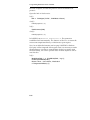
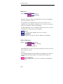
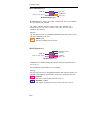
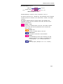
Now examine the Good PrimeQ.vi diagram, as illustrated in Figure
6, and run this VI. Again, before running the VI, make sure that your
kernel is not still connected to Bad PrimeQ.vi. In order to close the
connection, run Close All Links.vi (found in MLUtil.llb, or
accessible from the LabVIEW Tools menu). Although Good
PrimeQ.vi is similar to Bad PrimeQ.vi, because it uses an
uninitialized shift register to manage the session, the command it sends
to the kernel is very different. One evaluation only is sent:
PrimeQ/{random numbers}.
35
3 Getting Started
Elapsed Time
ms
Figure 6. The Good
PrimeQ.vi diagram.
1 [0..2]
A While loop introduced to use an uninitialized shift register
PrimeQ/@{
Data set size
}
,
1D Booleans
Range
5
Graph
The list is concatenated in the For loop
Test results
Because there are fewer MathLink transactions, Good PrimeQ.vi is
more efficient than Bad PrimeQ.vi – however, more effort is required
to properly format the command string. In order to quit, again run Close
All Links.vi (found in MLUtil.llb or accessible from the
LabVIEW Tools menu.)
Logs Description
Most packets received by LabVIEW are recorded in the log clusters. If
you are unfamiliar with MathLink, you only need to know that data
are sent over the link wrapped in packets. The “Packet log” maintains
an up-to-date accounting of packets received from the kernel. You can
ensure that the results of the previous request are returned by the kernel
prior to sending the next evaluation simply by monitoring the size of
the “Packet Log”. For a more detailed description of this cluster, see
“Packet Parser.vi” on page 89.
Numerical Data Types Compatibility
In contrast to Mathematica, numerical data type definitions have been
relaxed in the initialization of Kernel Evaluation.vi to make
handling numbers easier. In Mathematica integers, reals, rationals, and
36
Mathematica Link for LabVIEW
complex numbers are distinct because different Mathematical
properties hold for each of these types of numbers. In LabVIEW the
difference is not that dramatic—LabVIEW operators can handle the
three kinds of numbers without differentiation. For instance, the
number “2” is an integer and nothing else for Mathematica. In
LabVIEW it could be an integer, a real, or a complex number.
In addition, determining the correct data type that results from an
evaluation can be a tricky or even impossible exercise. What would be
the expected data type of I^2 or 1/2? In Mathematica, evaluating the
first one returns an integer and evaluating the second one returns a
rational. But for LabVIEW, the first one could be a complex number and
the second could still be regarded as a real number. Because of situations
like this, data type definitions were relaxed so as to allow coercion of
Mathematica data types into LabVIEW when possible without loss of
information. The following table shows the authorized correspondences
between Mathematica evaluation types and those you can select on the
Kernel Evalution.vi front panel.
Mathematica type
Valid Kernel Evaluation.vi types
Integer
Integer, Real, Complex
Rational
Real, Complex
Real
Real, Complex
Complex
Complex
Whatever the type of your result, you can select “Complex” in
Kernel Evalution.vi. But if your evaluation returns a real number
in Mathematica and you select “Integer” on the
Kernel Evalution.vi front panel, then you will be notified that the
result of your evaluation does not match the expected data type. This
rule can easily be extrapolated to lists and matrices of numbers.
Troubleshooting
1. LabVIEW cannot find the Mathematica kernel. If you are prompted
to locate a MathLink application to launch, this generally means
that your installation is not properly configured. One way to solve
the problem is to locate the kernel that you want and launch it
manually, however this is only a temporary solution. Another
option is to locate and open Launch Kernel.vi, then set the
MathKernel file path explicitly, as outlined on page 22. If you are
not comfortable with setting this parameter manually, reinstalling
Mathematica Link for LabVIEW using the VI-based installer
should alleviate further difficulties. (See Chapter 2).
37
3 Getting Started
2. The Mathematica kernel is already launched. You are notified of
this situation by a specific MathLink error message. You must quit
your Mathematica kernel before running Kernel Evaluation.vi
again. You can either quit it manually or run Close All Links.vi
(found in MLUtil.llb and accessible from the LabVIEW Tools
menu.)
3. The data type is incorrect. There are a number of situations that can
result in an unexpected data type. For instance, if you evaluate 10, a
symbol Null is returned instead of the integer that you may have
expected. Similarly, if you attempt to evaluate Table[Sqrt[i], {i,
10}], expecting a list of real numbers, you may be surprised to get an
error message saying that the returned data type does not match the
expected type. You must specify that you want the numerical value
of this list (using the Mathematica N[ ] command) to return a list of
real numbers.
4. The Mathematica kernel has quit. If you send an abort message to
the kernel while no evaluation is running it makes the kernel quit.
5. You want to use a remote kernel. Kernel Evaluation.vi cannot
launch a remote kernel. You can open a link to a remote kernel and
use Kernel Evaluation.vi on this link. For details on opening
links, consult “Getting Connected” on page 75.
Generic Plot.vi and Generic ListPlot.vi
Generic Plot.vi and Generic ListPlot.vi are a pair of VIs
designed to fulfill the most common needs of Mathematica graphics
presentation within a LabVIEW application. There are two important
areas where Mathematica can complement LabVIEW’s built-in data
visualization tools. These are functions that plot analytical functions,
which we refer to as “Plot functions”, and functions to visualize lists of
data, which we refer to as “ListPlot functions”. The VI that calls all
Plot functions is named Generic Plot.vi, and the one that calls all
ListPlot functions is named Generic ListPlot.vi.
Rendering graphics in Mathematica is somewhat more complicated
than evaluating a command that returns data, since it is necessary to
use an ancillary application named MLPost. Mathematica graphics are
PostScript graphics, which must be interpreted by a PostScript
interpreter application in order to be rendered on a computer monitor. In
the usual Mathematica configuration (i.e., the notebook front end
interacting with the kernel), the kernel returns the PostScript code to
38
Mathematica Link for LabVIEW
the front end before it is displayed in the notebook. Since neither
LabVIEW nor the kernel can interpret PostScript code, it is necessary to
call an external PostScript interpreter to generate a bitmap version of
the graphic that can be displayed in a LabVIEW window. MLPost is
the PostScript interpreter that performs this task. It is operated
through a MathLink connection directly managed from within
LabVIEW. The VIs of MLStart.llb take care of these issues for you,
but you should be aware of the function of MLPost, since you will see
that this application is launched when graphics are generated. You can
consult “Graphics Rendering” on page 92 for a more detailed description
of these issues. Another consequence of the use of MLPost is that there is
a significant delay in the generation of graphics. Also note that the
first call to MLPost takes additional time because the application must
be launched.
To integrate Mathematica graphics into LabVIEW VI front panels, the
bitmap images generated by MLPost are converted to a format
compatible with a specially-customized LabVIEW intensity graph. A
copy of this customized intensity graph named Graphics
Window.ctl can be found in MLStart.llb.
Use of Generic ListPlot.vi
Like Kernel Evaluation.vi, this VI can also function either as a
main application or as a subVI. Some advanced settings to optimize its
performance are discussed later in this section.
BASIC OPERATION
To run Generic ListPlot.vi, you will need to understand some of
the controls on the front panel shown in Figure 7. Above the box labeled
“Options” there is a pop-up control that can be used to select the type of
graphics you want to make with your data. Each type corresponds to a
particular Mathematica function: ListPlot, ListContourPlot,
ListDensityPlot, and ListPlot3D. (Refer to the Mathematica
documentation for an introduction to these functions if you are not
already familiar with them.) Each function uses a data array as its
first argument, followed by a series of options. Data are passed to the
VI as a LabVIEW array named “Data”, located below the “Options”
box: options are passed as a string. The controls, “Timeout“ and
“Resolution”, will be discussed later in “Advanced Settings” on page 41.
Fill the first column of the “Data” control with some data as shown in
Figure 7. To run the VI, first make sure that the Mathematica kernel is
not running by quitting it if necessary. You can either quit it manually or
39
3 Getting Started
use Close All Links.vi, (found in MLUtil.llb and accessible from
the LabVIEW Tools menu). Now click the Run button. Soon an
elementary plot will be rendered. Since this operation needs to launch
both the kernel and MLPost it may take longer than expected. (On
slower, older PCs, this may take as long as 20 or 30 seconds.)
Figure 7. Generic
ListPlot.vi
front panel.
Link in
1
Link out 1
MLPost link in
2
MLPost link out 2
error in (no error)
status
error out
code
no error
status
0
no error
source
code
7001
source
ListPlot
0
Timeout
Resolution
Options
30.00
s
300
PlotJoined->True, Frame->True
Data
0
0
10.00
0.00
20.00
0.00
If this step was successful, you can add additional plot options to the
evaluation. Plot options should be typed in the “Options” box, with
commas used for separation if several options are used in sequence.
However, option sequences should not be enclosed in braces, as they are
in the usual Mathematica syntax – nor should option sequences be
enclosed in quotation marks. Here are examples:
• Correct:
PlotJoined->True, Frame->True, PlotLabel->"My Plot"
• Incorrect:
{PlotJoined->True, Frame->True, PlotLabel->"My Plot"}
AN IMPORTANT NOTE ABOUT ASPECT RATIO
When using Generic ListPlot.vi the last item in the “Options” box
should always be AspectRatio-> 1. This ensures that the Mathematica
image will completely fill the LabVIEW intensity graph. If this step
is neglected, residual data may fill the unused portions of the intensity
graph, compromising the aesthetic quality of the visual presentation.
Feel free to experiment with your own data sets, but remember that not
all of the four ListPlot functions accept data with the same format.
40
Mathematica Link for LabVIEW
ListPlot is the most versatile, since it accepts data with two different
formats. For instance, ListPlot[{y1, y2, ..., yn}] plots y1, y2,..., yn
at x values 1, 2, ..., n. Yet, you can specify custom x values using the
alternative format for the data list: ListPlot[{{x1, y1}, {x2, y2}
...,{xn, yn}}].
Experiment with
Illustrate
ListPlot.vi to see
how different data
structures are used by
various functions for
data visualization.
In Tutorial.llb, you will find a VI named Illustrate
ListPlot.vi. This VI illustrates how different kinds of data
structures are used by the different ListPlot functions. Run this VI and
consult its diagram.
ADVANCED SETTINGS
Resolution. The bitmap version of the Mathematica PostScript
graphics is a square matrix of color values. The “Resolution” indicator
is used to control the size of this matrix. It specifies, in pixels, the size
of a side of the bitmap image. A low value will result in a crude
rendering and a high value uses a considerable amount of memory (the
picture size grows as the square of the resolution parameter). The
setting of this parameter is partly determined by the size of the control
in which the picture is displayed. For example, a value of 300 ensures a
nice display on the Generic ListPlot.vi front panel. The same
quality is achieved with a value of 200 in the smaller box of ListPlot
Benchmark.vi (see “Performance Evaluation” on page 42).
Timeout. This control specifies the maximum time that the VI will
wait for the result of a Mathematica evaluation, so that you can avoid
being trapped in a long or infinite Mathematica evaluation. If you do
not mind waiting a long time, give this parameter a high value. A high
value will not delay the evaluation: the result will be returned as soon
as it is available from the Mathematica kernel. If the time out is
exceeded before graphics are returned, the execution of the VI will stop
and nothing will be displayed.
Note that the time out applies only to the Mathematica kernel’s
evaluation time. It does not include the time required by MLPost to
interpret the PostScript. In order to estimate a reasonable value for the
time out parameter, you can make tests in the Mathematica front end to
gauge the time required for the computation of graphics that are
similar to the ones you plan to visualize in LabVIEW.
41
3 Getting Started
PERFORMANCE EVALUATION
Since rendering graphics can be computationally time-consuming, a tool
has been provided in Tutorial.llb to help you analyze how long it
will take on your hardware configuration: its name is ListPlot
Benchmark.vi.
ListPlot Benchmark.vi. is designed to generate a sequence of
graphical outputs, the number of which is set by an “Iteration” control
on the front panel. Data are generated by sinusoidal functions and
arranged in a matrix having “Line” lines and “Column” columns. You
can control the resolution of the display with the “Resolution” slider,
and there is also a control to select the type of plot you want to
generate. All of the graphics that are generated are stored in a buffer
and are displayed sequentially, once when they are computed and a
second time after the last iteration is completed. The second display
sequence indicates how the display step will perform on your system.
To get an idea of the time it takes the Mathematica kernel to create
the graphics, go to the Mathematica front end and execute the
following example commands:
l = Table[Cos[i] Sin[j], {i, 20}, {j, 20}];
Timing@ListContourPlot[l]
Close any link that may still be open with Close All Link.vi.
Create the same graphics with ListPlot Benchmark.vi, and
compare the time needed to render the graphics with the time that was
needed by Mathematica.
The most time-consuming step in the graphics rendering process is the
PostScript interpretation, and how long it takes depends on the
complexity of the graphic. Use ListPlot Benchmark.vi with
increasing numbers of columns and lines at a fixed resolution. You will
see that the iteration time depends more on the size of the data set
being plotted than on the resolution of the display. Also note that some
kinds of graphics are more complex than others. For instance, given 20
lines, 20 columns, and a 200–pixel resolution, it will take about twice as
long to evaluate ListContourPlot or ListPlot3D as it will to evaluate
ListDensityPlot.
42
Mathematica Link for LabVIEW
USE AS A SUBVI
ListPlot Benchmark.vi is an example of the use of Generic
ListPlot.vi as a subVI of an upper–level VI. Figure 8 shows how
Generic ListPlot.vi can be used in this context.
Iteration
ms
0
ms
Figure 8. The ListPlot
Benchmark.vi diagram.
Line
Column
0 [0..1]
Graph
10
Interpolate Color
Low Color
High Color
Color Array
Ignore Array
Resolution
Phase shift
Current error
status
Link out
Current error
1 [0..1]
43
3 Getting Started
Nothing is particularly challenging in this implementation except
perhaps the link management scheme. The simplest situation is one
where you have LabVIEW, MLPost, and the Mathematica kernel
running on the same machine with no other link active. Use an
uninitialized shift register for each link number so as to initialize the
connection when the VI is run for the first time. Then use the current
link numbers in subsequent evaluations. Since both the link to
Mathematica and the link to MLPost work in concert to render graphics,
you can bundle them together and use a single shift register for both of
them.
Generic Plot.vi
Generic Plot.vi is very similar to Generic ListPlot.vi. It too
can function as either as a stand-alone application or as a subVI. Some
advanced settings to optimize its performance will be discussed later in
this section.
BASIC OPERATION
Generic Plot.vi is a close relative of Generic ListPlot.vi. The
main difference between the two is that GenericPlot.vi does not use
a list of data as an argument. In order to provide the same level of
flexibility as the Mathematica syntax, the commands are passed as
strings to this VI—just as they are with Kernel Evaluation.vi
(discussed earlier in this chapter). You can use this VI to send any
sequence of commands that would return graphics from the kernel.
The “Command” box is used to type in the sequence of Mathematica
commands, so there is no need to have a separate window for options.
Options can be typed directly into the appropriate place in the
command string.
Although the name of this VI refers to plot functions, keep in mind that
there is little limitation to the form that plot functions may take. Any
functions that return graphical output can be typed here. This includes
low-level graphics primitive commands such as:
44
Mathematica Link for LabVIEW
Show@Graphics@{Dashing[{0.5, 0.5}],Line[{{-1, -1},{1, 1}}]}
or higher level command such as:
ListPlot[Table[Sin[i], {i, 0, 10Pi, Pi/5}]].
Generic Plot.vi is a general-purpose graphics generator that
contains, as a special case, the functionality of Generic
ListPlot.vi.
Examine the contents of the “Command” box in Figure 9. Two graphics
named p and q are generated first. Next,
Show@GraphicsArray[{{p}, {q}}]
produces the picture displayed in the figure.
Note: Intermediate commands must end in a semicolon to avoid a
premature exit from the evaluation.
AN IMPORTANT NOTE ABOUT ASPECT RATIO
When using Generic Plot.vi the last item in the “Command” box
should always be AspectRatio->1 . This ensures that the
Mathematica image will completely fill the LabVIEW intensity
graph. If this step is neglected, residual data may fill the unused
portions of the intensity graph, compromising the aesthetic quality of
the visual presentation.
ADVANCED SETTINGS
The “Timeout” and “Resolution” controls are analogous to the ones found
in Generic ListPlot.vi. Review “Advanced Settings” on page 41,
for a detailed description.
PERFORMANCE EVALUATION
Record the time required to evaluate the following commands from the
standard Mathematica front end:
• Plot3D[Sin[ x y], {x, 0, 2Pi}, {y, 0, 2}]
• ListPlot[Range[10]]
Close all the links that may still be open with Close All Link.vi
and run Plot Benchmark.vi. In this way you can evaluate the same
commands and compare the evaluation time to appreciate how
Generic Plot.vi performs on your system.
45
3 Getting Started
Figure 9. The Generic
Plot.vi front panel.
Link in
1
Link out 1
MLPost link in
2
MLPost link out 2
error in (no error)
status
no error
code
0
source
error out
status
no error
7001
source
Timeout (60s)
Command
code
Resolution
60.00
s
300
p=Plot3D[Sin[x y],{x,0,2}, {y,0,2}, AspectRatio->0.5];
q=Show[ContourGraphics[p],
ColorFunction->Hue,AspectRatio->0.5];
Show[GraphicsArray[{{p}, {q}}],AspectRatio->1]
In[1]:=
Show::gcc: Graphics of type -GraphicsArraycannot be combined with other types of graphics.
USE AS A SUBVI
Plot Benchmark.vi is an example of the use of GenericPlot.vi as
a subVI. Generic Plot.vi can be wired into a diagram in very much
the same way as Generic ListPlot.vi. Thus, see the discussion
pertaining to Generic ListPlot.vi under “Use as a SubVI” on page
43.
Plot Benchmark.vi has several features that have not been
discussed yet. First, it has a message box that displays Mathematica
messages. This is accomplished by a small algorithm that extracts the
last message generated by the kernel from within the message string
returned by Generic Plot.vi.
A “New session” button has also been introduced. When its value is
“True”, all active links are closed and two new links are opened to
MLPost and the Mathematica kernel. This strategy is somewhat crude,
but it is extremely easy to implement when no other links are being used
by an application.
46
Mathematica Link for LabVIEW
Troubleshooting
You are prompted to locate MLPost. This means that MLPost has not
been found. It is likely that the file structure of the MathLink
subdirectory of the user.lib directory has been changed. You can
either fix it as described in “The MathLink Subdirectory” on page 23, or
you can reinstall Mathematica Link for LabVIEW to correct the
problem.
The plot does not match the command. Sometimes the graphics
displayed by the VI are inconsistent with the sequence of commands
that were sent. This may occur when an error condition is
encountered—the graphic is not returned by the kernel, but rather is
queued on the link as a result of the error. (Note: graphics queued on the
Link will typically display during the next execution). If you encounter
this problem, the best solution is to reinitialize the links by running
Close All Links.vi (from MLUtil.llb or the Tools menu),
then rerun Generic Plot.vi.
MathLink VI Server.vi
MathLink VI Server.vi is a general-purpose utility that controls
LabVIEW VIs and applications from within a Mathematica notebook.
You typically would run this VI on the computer that is connected to
your instruments. The VI works in combination with the VIClient.m
package to provide “VI Server-like” control of LabVIEW VIs from
within a Mathematica notebook.
MathLink VI Server.vi first opens a link in Listen mode and waits
for Mathematica to connect. The VIClient.m package provides the
function ConnectToServer[ ] on the Mathematica side, which
automates the connection step. This connection, when established, is not
specific to the LabVIEW application; the link can be used to run any VI
or application saved on a volume accessible to the computer where
MathLink VI Server.vi is running. It can even manage several
VIs simultaneously.
47
3 Getting Started
Figure 10. The MathLink
VI Server.vi front panel.
Scan period (1s)
1.00
s
Delay to stop
1.00
s
Connected
Link ID 0
error out
Link name
5555
status
no error
Link mode
Listen
code
0
source
Link protocol
TCP
VI location
Macintosh HD:LabVIEW:
examples:app:Tempsys
demo.vi
Current Command
CallInstrument
RunInstrument
PreloadInstrument
ReleaseInstrument
OpenPanel
The VIClient.m package’s main functions are basic: to load a VI into
memory, to release it after use, to manipulate its front panel, and to run
it. The basic function set does not allow arguments to be passed to a VI,
nor can data be collected after the VI’s execution. However, another
function based on the similarly named VI Server function,
CallByReference[ ], allows parameter passing through VI controls, as
well as the return of VI indicator values after execution. (The
CallByReference[ ] command will be discussed in more detail later in
this section.)
Front Panel Organization
The MathLink VI Server.vi front panel is divided into three areas,
as shown in Figure 10. In the upper-left area are the controls used to set
the connection parameters. They include the protocol used, the
connection mode, and the default link name.
The link status indicators can be found in the upper-right area. An LED
titled “Connected” indicates whether the link is connected. An error
cluster is used in a standard way to report errors, and a digital indicator
displays the current link number.
In the lower part of the front panel, two boxes provide feedback on the
current VI’s operation. The “VI location” box displays the path or name
48
Mathematica Link for LabVIEW
of the VI being operated, and the current operation is highlighted in
the “Current command” box.
Using MathLink VI Server.vi
The material in this section is an extension to the material introduced
in Hands-on Tutorial #1 and #2 (as noted at the beginning of this
chapter). If you haven’t worked through these exercises, you may want
to look at them before continuing.
MathLink VI Server.vi operates in a three-phase operational
sequence: First, you must connect to it. Second, you need to declare
Instrument objects in Mathematica. Finally, you have to use the
functions of the VIClient.m package to operate LabVIEW
applications. We will explore each phase sequentially next.
GETTING CONNECTED TO THE SERVER
The first step in connecting to the VI server is to load the VIClient.m
package. The following command will load the package:
In[1]:=
<<LabVIEW`VIClient`
The VIClient.m package has a function that automates the connection
to MathLink VI Server.vi. It is named ConnectToServer. When
queried, Mathematica returns the following information about
ConnectToServer:
In[2]:=
?ConnectToServer
ConnectToServer[linkname, opt] is used to
establish a connection to the MathLink VI
Server.vi. Linkname is an optional
argument. When it is not specified, the
default linkname is set to "5555" and the
default protocol used is "TCP".
Mathematica and
LabVIEW run on a
single PC configured
to use TCP/IP.
If the TCP protocol is properly configured on your machine, and if
Mathematica and LabVIEW are running on the same machine, use the
following procedure to get connected. Open MathLink VI Server.vi
and click the Run button without changing any control value. Then go
back to the standard Mathematica front end to establish the
connection.
49
3 Getting Started
In[3]:=
link = ConnectToServer[ ]
Out[3]=
LinkObject[5555, 2, 2]
This output depends on your system configuration. In particular the
address of your local machine can be joined to the link name. In this case
the first argument of LinkObject is of the form 5555@machine address.
Running Mathematica
and LabVIEW on
different systems over
a TCP/IP network.
Running Mathematica
and LabVIEW under the
same platform using
the local protocol.
If you are running LabVIEW on a remote machine with TCP, you should
specify the address of that machine with the LinkHost option for
ConnectToServer (see below). You can also specify the machine address
in the link name using a name of the form 5555@machine address.
If your machine is not configured to use TCP/IP, use the local protocol.
On the MathLink VI Server.vi front panel select the local protocol
with the “Link protocol” control. The local procotol is “FileMap” on
Windows systems and “PPC” on Macintosh systems. Then click the Run
button without changing any other control value. Go back to the
standard Mathematica front end to establish the connection with the
following command.
link = ConnectToServer[ LinkProtocol->Automatic]
Generally, an appropriate choice of options needs to be specified to
make the connection possible. If you experience difficulties in your first
attempts, try using the local protocol as noted in the previous
paragraph. For more details about the options needed to open a link,
consult “Getting Connected” on page 75.
The next command reveals that the options for ConnectToServer
(introduced above) have the same names as those for LinkOpen, but
they have different values.
In[4]:=
Options[ConnectToServer]
Out[4]=
50
Mathematica Link for LabVIEW
{LinkMode -> Connect, LinkProtocol -> TCP,
LinkHost -> }
Note: On a MacOS
computer when the
MathLink VI
Server.vi is run,
LabVIEW may hang.
To solve the problem
see pages 75 and 27.
Note also that ConnectToServer returns a LinkObject just as
LinkOpen does. The main difference between the two functions is that
ConnectToServer has default option values that allow the remote
control of a LabVIEW application by Mathematica. Be aware,
however, that the default value of the LinkHost option is an empty
string as it is for LinkOpen. This is because relevant values depend on
your specific network configuration. To establish an operational
MathLink link, you must connect the link with the LinkConnect
function after declaring the link with the LinkOpen function.
ConnectToServer proceeds to this connection step before returning the
LinkObject. Thus, the LinkObject returned by ConnectToServer must
not be connected again—such as would be the case if LinkOpen returned
it.
INSTRUMENT DECLARATION
Once the connection has been established you must describe the
instrument—or more specifically, the VI you intend to operate. A
function named DeclareInstrument is provided for this purpose. It
returns an object of the type Instrument. This function usually requires
three arguments. The first is the path (including filename) to the VI
you want to run. The second is a list describing the controls of the target
VI, as well as their values. The last argument is used to describe the
indicators that you want to read. These topics will be discussed in “The
CallInstrument Function and Related Functions”on page 56. For right
now, we will only use the smallest set of arguments needed to declare an
instrument. The VI we will use in this section is Frequency
Response.vi, a standard example in the LabVIEW distribution.
The instrument declaration step takes the following form:
In[5]:=
inst = DeclareInstrument["HD:LabVIEW:examples:apps:
freqresp.llb:Frequency Response.vi"]
Out[5]=
Instrument[HD:LabVIEW:examples:apps:freqresp.llb:Frequency
Response.vi, Frequency Response.vi, {}, {}]
The preceding example specifies the VI path information for a typical
Macintosh configuration. When you reproduce this command on your PC,
51
3 Getting Started
do not forget to modify the path so that it leads to Frequency
Response.vi in your file system. For example, here is its adaptation
for a typical Windows configuration:
Confused by the
doubled path delimiters?
This Mathematica for
Windows convention
will be discussed
further in a moment.
inst = DeclareInstrument["C:\\LabVIEW\\examples\\
apps\\freqresp.llb\\Frequency Response.vi"]
As mentioned previously, the result returned by DeclareInstrument is
an Instrument object. This indicates that your DeclareInstrument
arguments are valid. A formal verification of the function arguments is
conducted by the DeclareInstrument function before returning the
resulting Instrument (consult “The VIClient.m Package” on page 201 for
details). The output in the preceding example may not appear on your
system; in fact the output that you do get may be different from what
you normally receive. For instance, in the example output, the path
string has at least one path delimiter character. This delimiter may be
not the one you expect from the operating system under which
Mathematica is running. Since the LabVIEW application you are
controlling may be remotely implemented, the path name separator
used by DeclareInstrument may not have the same value as the system
variable $PathnameSeparator. DeclareInstrument has an option
named PathnameSeparator that you can use to adjust this effect to your
liking. As an example, the next command declares, on a Macintosh or
other type of machine, a VI located on a UNIX machine with the
PathnameSeparator set to a “/”.
In[6]:=
inst2 = DeclareInstrument["~/readme.vi",
PathnameSeparator->"/"]
Out[6]=
Instrument[~/readme.vi, readme.vi, {}, {}]
In Windows, the path separator is the backslash character, “\”. This
is a potential source of confusion, since “\” is also a control character
used by Mathematica to format strings. For instance, “\t” is a tab and
“\r” is a carriage return. The string “\\” represents a single \ because
the first \ is the Mathematica control character that specifies the
interpretation of the second one. This is familiar to users who run
Mathematica under Windows, but might be puzzling to people used to
running Mathematica on other operating systems. To illustrate further,
here is another declaration example for a VI located on a Windows
machine:
52
Mathematica Link for LabVIEW
In[7]:=
inst3 = DeclareInstrument["C:\\LABVIEW\\README.VI",
PathnameSeparator->"\\"]
Out[7]=
Instrument[C:\LABVIEW\README.VI, README.VI,
{}, {}]
BASIC OPERATION
The VIClient.m package has a large number of functions that perform
basic operations on remote VIs. In order to maintain both backward
compatibility, and consistency with evolving LabVIEW nomenclature,
each function is defined by two different terminology sets. The first
terminology set is analogous to the VIs of victl.llb. Long-time
LabVIEW users with experience using the functions in victl.llb
should feel comfortable using the corresponding Mathematica
terminology. The other function set is patterned after the VI Sever.
Users coming to LabVIEW after the release of version 5.0 will likely be
more comfortable with the VI Server-compatible function set. The
functions sets are completely inter-changeable, so feel free to use the
function set which is most comfortable for you. Alternatively, if you
have no experience with either the traditional victl.llb VIs
(LabVIEW 4.1 and earlier), or VI Server functions (LabVIEW 5.0 and
above), you are encouraged first to have a look at the examples
provided with LabVIEW.
The advantage of using declared instruments is that you can now use a
variable to refer to the instrument. Note, however, that to operate the
instrument you need information both about the Instrument itself, and
about the link where the instrument will be addressed. None of the
basic operations return data (data exchange will be addressed a little
later in this discussion), so to acknowledge the receipt of your
instructions, the VI server will send you a message saying that the
operation was completed or that an error occurred.
Start by loading a VI from disk into memory.
In[8]:=
OpenVIRef[link, inst]
or alternatively (using the victl.llb terminology):
53
3 Getting Started
PreloadInstrument[link, inst]
Mathematica will respond with:
Frequency Response.vi loaded
While this command is being processed nothing is visible unless you use
LabVIEW tools to inspect VIs that are in memory (the VI hierarchy
tool or the Unopened subVIs item of the Windows menu).
You can now display the VI front panel.
In[9]:=
OpenPanel[link, inst]
Frequency Response.vi: panel displayed
Now you should see the VI panel and you can make an attempt to run
the VI.
In[10]:=
RunVI[link, inst]
or alternatively (using the victl.llb terminology):
RunInstrument[link, inst]
Frequency Response.vi running
Next, you can close the panel.
In[11]:=
ClosePanel[link, inst]
Frequency Response.vi: panel closed
The last operation that you can do with the basic functions of the
VIClient.m package is to release a VI from memory.
In[12]:=
CloseVIRef[link, inst]
or alternatively (using the victl.llb terminology):
ReleaseInstrument[link, inst]
54
Mathematica Link for LabVIEW
Frequency Response.vi released
Now go into LabVIEW to make sure that Frequency Response.vi
has been removed from the VI hierarchy.
To gain further understanding of these tools it might be useful to enter
some commands that give rise to errors. Start by declaring an instrument
that is not on the hard drive.
In[13]:=
fooinst = DeclareInstrument[":foo.vi"]
Out[13]=
Instrument[:foo.vi, foo.vi, {}, {}]
In[14]:=
OpenPanel[link, fooinst]
Error 1004
Error 1004 occurred at VI not in memory.
Possible reasons:
LabVIEW: The VI is not in memory.
This is a very reasonable reply: the VI has not been loaded. So, you can
try to load it.
In[15]:=
OpenVIRef[link, fooinst]
Error 7
Error 7 occurred at VI not found at path.
Possible reasons:
LabVIEW: File not found.
OR
NI-488: Non-existent board.
Here again, you can rely on the error message returned to Mathematica.
SERVER REMOTE SHUTDOWN
The last basic function of the package is named ServerShutdown, and
it is used to close the link and stop the remote VI server. Since it is not
instrument specific, its only argument is a link to the server.
There is no specific button on the server panel to stop the VI. The reason
is that only the client should be able to decide when the service is not
55
3 Getting Started
needed anymore. There is no indication on the MathLink VI
Server.vi panel that it is currently used by someone when it is
connected. Stopping the server in LabVIEW is not advisable, although
it is possible with the Abort button on the VI’s toolbar. If you use this
method, make sure to close the link manually, either with Close All
Links.vi, or with MLClose.vi.
Here is the correct way to use ServerShutdown to close the link.
In[16]:=
ServerShutdown[link]
Out[16]=
Server stopped
THE CALLINSTRUMENT FUNCTION AND RELATED FUNCTIONS
The aforementioned basic functions do not allow execution parameters
to be passed to and from LabVIEW. However, VI Server and the
victl.llb have more general methods that are capable of passing
control values to VIs and collecting indicator values. The VIClient.m
package taps into this functionality with 2 interchangeable functions:
CallInstrument—consistent with victl.llb terminology, and
CallByReference—consistent with VI Server terminology. We will
look at these interchangeable functions in context next.
First, before we can call a VI to exchange data, we must declare it. And
if we want to access the controls and read the indicators, we also must
declare the controls and indicators of interest in the DeclareInstrument
command. Apart from the path to the VI, two other arguments are
necessary. The first argument is a list of controls: each control must be
described by its name, data type, and value. The indicators that you
want to read are specified in the second list. Naturally, you do not
have to provide indicator values (these will be returned at run-time),
however, you must provide the name and type for each indicator of
interest. Here is an extension of the example used in the previous
section:
In[17]:=
inst = DeclareInstrument["HD:LabVIEW:examples:apps:
freqresp.llb:Frequency Response.vi", {{"Amplitude", DBL,
1.5}, {"Number\nof Steps", I32, 20 }}, {{"Current
Frequency", DBL}}]
Out[17]=
56
Mathematica Link for LabVIEW
Instrument[HD:LabVIEW:examples:apps:freqresp.llb:
Frequency Response.vi, Frequency Response.vi,
{{Amplitude, DBL, 1.5},
{Number
of Steps, I32, 20}},
{{Current Frequency, DBL}}]
Important note:
control and indicator
names must be
entered as they appear
on the VI diagram.
Read this output carefully. The second control is named “Number\nof
Steps”. Why is it necessary to place the “\n” between “Number” and
“of”? The answer lies in the VI diagram. Whereas the control label is
written on a single line on the front panel, it is written on two lines in
the diagram. If you do not introduce the “\n”, the Mathematica
newline character, in the control name, Call Instrument.vi will not
recognize it.
You can easily query Mathematica to access the list of data types
supported by the DeclareInstrument function.
In[18]:=
SupportedTypes[]
Out[18]=
{EXT, DBL, SGL, I32, I16, I8, U32, U16, U8,
CXT, CDB, CSG, EXTList, DBLList, SGLList,
I32List, I16List, I8List, U32List, U16List,
U8List, CXTList, CDBList, CSGList,
EXTMatrix, DBLMatrix, SGLMatrix, I32Matrix,
I16Matrix, I8Matrix, U32Matrix, U16Matrix,
U8Matrix, CXTMatrix, CDBMatrix, CSGMatrix,
Boolean, BooleanList, BooleanMatrix, String,
StringList, StringMatrix}
These are all the types of LabVIEW numbers, strings, and booleans, plus
one-dimensional and two-dimensional arrays of these types of data. If
you are not familiar with these data types, each one is briefly
57
3 Getting Started
documented on line. Information for each data type can also be obtained
using the Mathematica query operator. Here is an example.
In[19]:=
?CXT
LabVIEW data type: complex extended-precision
floating point number.
You can also refer to the LabVIEW documentation for more details.
Now connect to the VI server once again. Go into LabVIEW, run
MathLink VI Server.vi, then go back to Mathematica to get
connected and to call the instrument. Type the following commands:
In[20]:=
link = ConnectToServer[ ]
Out[20]=
LinkObject[5555, 3, 2]
In[21]:=
CallByReference[link, inst]
or alternatively (using the victl.llb terminology):
CallInstrument[link, inst]
Frequency Response.vi successfully operated.
Out[21]=
1000.
When you need to run a
VI several times with
CallByReference ,
use OpenVIRef first.
Before the result is returned you will observe the VI loading (actually,
you will hear the disk drive). You will see it briefly running and then it
will be released from memory. This behavior is described in the Call
Instrument.vi on-line documentation.
If you preload the VI or open a VI reference first, the VI is less likely to
vanish at completion. (The rules defining when and how VIs are closed
and unloaded from memory is beyond the scope of this discussion. Refer
to VI Server topics in the LabVIEW documentation for more
information.)
To open a VI reference or ‘preload’ the VI before calling it by reference,
use the following command sequence:
58
Mathematica Link for LabVIEW
In[22]:=
OpenVIRef[link, inst]
or alternatively (using the victl.llb terminology):
PreloadInstrument[link, inst]
Mathematica responds with:
FrequencyResponse.vi loaded
Continue with:
In[23]:=
OpenPanel[link, inst]
FrequencyResponse.vi: panel displayed
In[24]:=
CallByReference[link, inst]
or alternatively (using the victl.llb terminology):
CallInstrument[link, inst]
After the VI terminates, Mathematica responds with:
Frequency Response.vi successfully operated.
Out[24]=
1000.
Since you will use the CallByReference and/or the CallInstrument
functions to operate VIs, you need a convenient way to interactively
edit instrument values. Three functions are provided for this.
• SetControls: The function used to change the value of a list of
declared controls.
• AddControls: The function used to add new controls to a
declared instrument ‘s current list of controls.
• AddIndicators: This function is the same as AddControls,
except that it applies to indicators.
Test these functions in conjunction with the CallByReference function.
To make the exercise more fun, use a different example VI. (Remember
to set the path appropriately for your own file system.)
59
3 Getting Started
In[25]:=
echo =
DeclareInstrument["HD:LabVIEW:examples:analysis:
dspxmpl.llb:Echo Detector"]
Out[25]=
Instrument[HD:LabVIEW:examples:analysis:
dspxmpl.llb:Echo Detector, Echo Detector, {}, {}]
In[26]:=
OpenVIRef[link, echo]
Echo Detector loaded
In[27]:=
RunVI[link, echo]
Echo Detector running
In[28]:=
echo = AddControls[echo, {"Samples", U16, 1}]
Out[28]=
Instrument[HD:LabVIEW:examples:analysis:
dspxmpl.llb:Echo Detector, Echo Detector,
{{Samples, U16, 1}}, {}]
In[29]:=
echo = AddControls[echo, {"Frequency", DBL, 45.0}];
In[30]:=
echo = AddIndicators[echo, {"Echogram", DBLList}];
In[31]:=
echo
Out[31]=
Instrument[HD:LabVIEW:examples:analysis:
dspxmpl.llb:Echo Detector, Echo Detector,
{{Samples, U16, 1}, {Frequency, DBL, 45.}},
{{Echogram, DBLList}}]
In[32]:=
data = CallByReference[link, echo][[1]];
60
Mathematica Link for LabVIEW
Echo Detector successfully operated.
In[33]:=
ListPlot[data, PlotJoined->True, Frame->True, PlotLabel>"Experimental echo"];
Experimental echo
0
-1
-2
-3
-4
-5
-6
0
100
200
300
400
500
Thus, you now have access to experimental data from within
Mathematica notebooks. Close the link with ServerShutdown.
In[34]:=
ServerShutdown[link]
Server stopped
Consult “The VIClient.m Package” on page 201 for a more detailed
description of VIClient.m package functions.
Main Limitations of VIClient.m Functions
• From within Mathematica you can only operate VI controls
belonging to a limited set of data types: numbers of all kinds, strings,
booleans, and lists and matrices of these basic data types. You
cannot, for instance, set the value of a cluster control. However, you
still can run these VIs with the current values of the controls
(default values or values set manually). Moreover, the ‘to array’
and ‘from array’ functions usually make it easy to convert clusters
into list of numerical data.
• Many LabVIEW applications can be considered as process
monitoring applications. They continue to run and monitor a process
61
3 Getting Started
until the operator stops them (by clicking a Stop button, for
instance). There is no function in the VIClient.m package to
dynamically collect the data recorded by these kinds of
applications. It is possible to run them, but no data will be returned,
and the application needs to be stopped manually. In this kind of
situation, you should introduce a small MathLink subVI in your
application to manage communication with Mathematica at run
time. Examples are provided in “Process Monitoring with
MathLink” on page 107.
• It is not possible to stop the VI server in LabVIEW if it has not been
connected. To stop it, go into Mathematica and connect yourself to
the server, then shut it down.
MathLink and Mathematica Link for
LabVIEW
In order to use Mathematica Link for LabVIEW effectively, a basic
understanding of its foundations is helpful. In this section, the global
architecture of the package is described. A brief introduction to the
differences between Mathematica and LabVIEW with respect to data
management is also necessary to understand how data are transferred
between Mathematica and LabVIEW using Mathematica Link for
LabVIEW.
Software Architecture
Mathematica Link for LabVIEW is a straightforward LabVIEW
translation of the C functions of the MathLink library. Each MathLink
VI implements a single MathLink function. So, for instance, you will
find in your distribution MLOpen.vi, MLPutInteger.vi, and so on.
However, not all of the VIs of your Mathematica Link for LabVIEW
distribution are MathLink VIs. Several libraries provide utilities or
high-level VIs, which have no direct MathLink counterparts.
All the VIs implementing MathLink functions make use of a subVI
named MathLinkCIN.vi. MathLinkCIN.vi is the only VI in the
distribution that contains a LabVIEW Code Interface Node (CIN). This
CIN can be regarded as the heart of the software, since this is the
interface point where MathLink functions are called. To some extent,
this VI can be viewed as a Mathematica–LabVIEW translator.
Mathematica can maintain a dialog with the C program through
MathLink. This C program can also carry on a dialog with LabVIEW
62
Mathematica Link for LabVIEW
through a Code Interface Node. Thus, Mathematica and LabVIEW can
exchange information through MathLink and a Code Interface Node.
Figure 11. The global
structure of Mathematica
Link for LabVIEW.
LabVIEW Application
MathLink VIs
MathLinkCIN.vi
LabVIEW
hierarchical
design
Code Interface Node
A second link is used to send
PostScript graphics to MLPost
and to read the bitmap
version of the picture .
MLPost
Evaluation parameters and
evaluation results are transmitted
over the link to the kernel.
Mathematica kernel
The global structure of Mathematica Link for LabVIEW is illustrated
in Figure 11. A LabVIEW application can use MathLink functions by
using VIs that implement those MathLink functions. These VIs
themselves call the CIN-containing VI, MathLinkCIN.vi. The
external C code is where the actual MathLink functions are called.
Three Sets of Data Types
In order to avoid confusion, you must keep in mind that, when you use
Mathematica Link for LabVIEW, three programming languages are
working together, each having its own set of data types.
Mathematica data are mainly expressed as compound expressions
composed of atoms belonging to a limited set of atomic data types. The
types are Symbol, String, Integer, Real, Rational, and Complex.
Note that Number is not one atomic type, but rather, the union of the
63
3 Getting Started
last four types. (Refer to sections A.1.4 and A.1.5 of “The Mathematica
Book”, by S. Wolfram [6] for more details.)
Similarly, LabVIEW has its own set of elementary data types. This
set is much larger (26 elementary types) than the Mathematica set of
atomic types. (Consult the LabVIEW documentation for an exhaustive
list of LabVIEW elementary data types. ) Regarding complex data
types, LabVIEW handles them either as “Arrays”, “Clusters”, or any
combination of both (cluster of arrays, array of clusters, and so on).
Arrays are multidimensional, but must contain elements of identical
type, whereas clusters are a means of combining data of different types
into a single structure.
Data are transferred between Mathematica and LabVIEW by a layer of
C code having its own data structures and types. Any textbook on the C
programming language will give you details about C data types. But
you do not need to have any experience programming in C to use
Mathematica Link for LabVIEW—the data you exchange over the
link between Mathematica and LabVIEW are transparently handled
by MathLink functions.
Polymorphism
When designing your programming project, you have to consider the
kind of relationships you will define between the elementary programs
written with the language you are using, and the data that they
manipulate. Some languages allow you to build programs capable of
using several types of data as arguments; the data type they return
depends on the kind of argument they are supplied. Programs that
have this feature are said to be “polymorphic”. Nonpolymorphic
programs are “typed” programs.
LabVIEW, Mathematica, and C approach the issue of polymorphism in
very different ways. Mathematica is polymorphic by nature. Among
the simplest of Mathematica programs is the function f, defined by
f[x_] := x
Although it looks trivial, the fact that a programming language can
allow the definition of such a function is quite remarkable. It can use
anything as an argument and, thus, return any kind of data. In
Mathematica you can use pattern matching to restrict function
definitions to particular patterns. But be careful; patterns are not data
types. (Patterns represent a much subtler notion, which is part of the
foundation of symbolic computation.) Even so, you can shape patterns so
that they fit some types of data. For example,
64
Mathematica Link for LabVIEW
g[x_Integer] := x^2
h[x_^n_Integer] := n
SetAttributes[h, HoldAll]
The definition of g uses a pattern to limit its evaluation to integers, and
when it executes, it returns an integer. Thus, defined this way, g is a
typed function. Is the same also true for h? Certainly not. The pattern
used to define h ensures that only integers will be returned by this
function, but the kind of arguments it can use does not fit a single type of
data. The pattern only specifies that it must be something with an
integer power: the “something” can really be anything. Try it with x =
2, 2.5, a/b, 2/3, “foo”, or whatever else you can dream up. (The final
command, SetAttributes[h, HoldAll], is present so that the argument
of h will not be evaluated before the integer n is extracted.)
Polymorphism in LabVIEW can be misleading if you do not pay careful
attention to it. As you may know, many LabVIEW functions are
polymorphic. To illustrate this point, simply refer to the on-line
description of the Add operator function: the inputs can be any type
of number, a number and an array of numbers, and so forth. The data
type that is returned depends on the data types of the inputs. The fact
that most built-in functions are polymorphic to varying degrees does not
mean that they share this feature with LabVIEW programs, that is
VIs. VIs are not polymorphic. When you build a VI, you have to specify
the types of all the controls and indicators you use: your inputs and
outputs. This also applies to complex data structures such as arrays and
clusters. Even the polymorphic VI feature introduced in LabVIEW 6
requires duplicate versions of a VI to be constructed—one for each data
type supported. Here again, it is also worth noting that there is no way
in LabVIEW to programmatically control the data structure of the
inputs and outputs of a VI. You cannot add an indicator at run time or a
dimension to a front panel array, or an element to a cluster control. Thus,
we can say that despite the polymorphism of its built-in functions, and
some recent additions to simulate polymorphic behavior, LabVIEW
remains a typed language.
The C language is not polymorphic at all (although the object-oriented
language C++ is). When defining a function in C, you need to carefully
specify the type of each argument as well as the type of the value
returned by the function. To understand how strict the various
MathLink functions definitions are, consult Section A.11 - “Listing of C
Functions in the MathLink Library” in “The Mathematica Book” [6].
65
3 Getting Started
Type Casting
Another notion, “type casting”, also deserves clarification. Type
casting is a mechanism to coerce a variable of one type into another
type. Type casting provides a conversion mechanism for the data; that
is, a transformation of the data from one type to another. For instance,
you can cast a real value into an integer type, but this process is not
reversible, since the number has been rounded during the first
conversion. When a function is polymorphic it does not need to use type
casting, since the function is defined for different data types. However,
many LabVIEW functions are still not polymorphic, so type casting can
occur frequently, especially for numerical variables. LabVIEW notifies
you that type casting will occur by way of coercion dots on the diagram.
Type casting can be kept to a minimum by eliminating coercion dots
wherever possible.
Elementary Data Type Conversion Table
The following table shows the most natural correspondences between
the elementary data types of the three languages.
Mathematica
MathLink
LabVIEW
Integer
short integer, integer, long
integer
I8, I16, I32, U8, U16, U32
Real
double, long double
SGL, DBL, EXT
Complex
Mathematica expression
CSG, CDB, CXT
Rational
Mathematica expression
SGL, DBL, EXT
String
string
abc
Symbol
string
abc
In this version of Mathematica Link for LabVIEW, extended precision
numbers are converted to double precision numbers and word integers
(16-bit format) are converted to long integers (32-bit format) for
MathLink transactions. While this should prove adequate for the
majority of practical implementations, future versions of the Link may
introduce additional data formats.
Peculiarities of Mathematica Link for LabVIEW
Every effort was made during the development of Mathematica Link
for LabVIEW to retain 100% compatibility with the original
MathLink functions. However, differences between LabVIEW and the C
language make minor adaptations of some MathLink features
66
Mathematica Link for LabVIEW
unavoidable. Specifically, MathLink VIs differ from their C
counterparts with respect to link identification, the way they
deallocate memory, and the way they report function values. MLOpen
uses front panel lists to specify its options. Also, VIs are not installable
in Mathematica.
Link in and Link out
No special MLINK data type has been defined in this distribution.
Links are simply identified by an I16 integer. Most VIs have both a
“Link in” control and a “Link out” control that can be used to force data
dependency and “chain” MathLink session VIs across the diagram. The
“Link out” value is the same as the “Link in” value. Both can be used to
create an artificial data dependency to ensure proper sequencing of
operations—a standard LabVIEW convention used with several builtin functions and libraries of the standard LabVIEW distribution (File
I/O, VI Server functions, TCP, UDP, PPC, etc.).
Function Value
Many MathLink functions return an integer that is used to indicate a
possible error. This integer is returned in a particular indicator named
“value” that all MathLink VIs have on their front panel. In the
MathLink VI diagrams, the integer error code returned by the
MathLink function call is checked by ErrorClusterMaker.vi. In case
it matches a value indicating an error, ErrorClusterMaker.vi will
build an error cluster indicating that an error occured (see “Introduction
to Error Management”, page 68 and “Error Management Tools", page 84).
Disown Functions
MathLink has a set of functions to free memory after arrays of data
have been read: MLDisownIntegerList, MLDisownString, and so
forth. Since these memory management issues would have looked
somewhat out of place in the LabVIEW environment, the disown
functions are automatically called whenever they are required in the
CIN. This means that you can get lists of any kind of data safely
without concerning yourself with memory management. Although it is
clearly specified in the MathLink documentation that you must call
MLDisownString after a call to MLGetString, in LabVIEW you can
read your string with MLGetString and forget the disown function.
This also applies to all of the functions that you use to get arrays of any
type.
67
3 Getting Started
MLOpen Arguments
The original prototype of MLOpen is MLINK MLOpen(argc, argv). It
is difficult to use that model to build a LabVIEW VI. Actually the four
arguments of MLOpen are the link mode, the link protocol, the link
name, and the link host. Two menus help you select the mode and the
protocol you want to use and two string controls specify the name and
address of a remote partner.
MLOpen returns an integer in “Link out”. The convention is that, in the
case of an error, 0 will be returned instead of a NULL pointer.
Noninstallable VIs
LabVIEW programs using MathLink are not installable in
Mathematica.
Introduction to Error Management
Error management in MathLink is a three-step process. First, most
MathLink functions return an integer value that can give you an
indication of the result (successful or not) of the execution. When zero is
returned, it means that an error occurred. You then have to call the
MLError function to know precisely which error occurred.
(Alternatively, you can call MLErrorMessage, for a user-friendly
description that is more useful than numerical error codes.)
Second, once you know precisely what happened, you can conduct the
most appropriate corrective action. Finally, you need to reactivate the
link with MLClearError.
LabVIEW also has a well-defined strategy for managing errors. (If you
are not familiar with this topic, you may also want to refer to
LabVIEW’s documentation.) A short overview of LabVIEW error
management is presented next.
In LabVIEW, error management in sequential I/O operations—such as
file manipulations or any kind of communication—relies mainly on
error clusters (Error In.ctl and Error Out.ctl) located in the
“Error Cluster” area of the Control menu. These clusters comprise three
elements: a boolean named “status” indicates whether an error occurred,
an integer is used to report the error code, and a string field named
“source” is used to report where the error occurred.
There are two families of I/O VIs, depending on their use of error
clusters; some use error clusters (VIs of DAQ libraries, VIs of tcp.llb),
68
Mathematica Link for LabVIEW
and some do not (VIs of the GPIB libraries, Serial.llb, and so on).
Those that do not use error clusters only return error codes, and it is your
responsibility to manage them safely. On the other hand, VIs that
take advantage of error clusters have an extremely clear errormanagement scheme. They first check the cluster status. If a preexisting error is detected, no other operation is undertaken in the VI.
“Error in” and “Error out” clusters are thus used to chain the VIs that
implement the sequence of operations. At the end of the sequence, you
can simply wire one of the LabVIEW error handlers to
programmatically control error management. Doing so ensures that not
more than one error can accumulate during a sequence of operations,
thereby simplifying troubleshooting operations.
All Mathematica Link for LabVIEW VIs employ error clusters except
those that do not return error codes (MLClose.vi and MLReady.vi, for
instance). You should always wire a MathLink Error Manager.vi
at the end of the MathLink operation chain; this is where MLError
and related functions are called.
69
4 Programming
Mathematica Link for LabVIEW
The Link Structure Revisited
The structure of the link between Mathematica and LabVIEW was
introduced in Chapter 3. In this first section on Link programming, the
organization of Mathematica Link for LabVIEW components is
described in more detail to help MathLink programmers develop their
own applications.
The Use of MathLinkCIN.vi
MathLinkCIN.vi is the central component in the Mathematica Link for
LabVIEW package. Its front panel is shown in Figure 12. It is a simple
VI that has two clusters: a control cluster for input called “Input
cluster”and an indicator cluster “Output cluster”. These clusters are
identical and have been designed to pass data used by MathLink
functions. MathLinkCIN.vi is saved in MLComm.llb.
The Copyright Notice.vi is a subVI of MathLinkCIN.vi. It is
thus executed once every time the CIN is called. Since the graphic
displayed by the Copyright Notice.vi subVI changes randomly at
Use keyboard shortcuts run time, it can be used to visually monitor the link activity. Note,
to hide the front panel however, that this display of graphics may use some CPU time and be
of Copyright
limiting in some circumstances. There are two ways to hide the front
Notice.vi.
panel of Copyright Notice.vi. It can be closed by the keyboard
shortcut Control+w ( command+w on the Macintosh), or you can simply
unselect the option “Show front panel when loaded” in the VI setup
menu.
4 Programming Mathematica Link for LabVIEW
MathLink communication interface
Figure 12. The
MathLinkCIN.vi
front panel.
Input
Output
cluster
cluster
MLFunction
MLFunction
Link in
0
Link out
0
Value
0
Value
0
long integer
0
string
string
long integer
0
double
0.00
double
0.00
long double
0.00
long double
0.00
integer list
0
long integer list
0
double list
long double list
0
0
0
integer list
0
0
0
long integer list
0
0
0.00
double list
0
0.00
0.00
long double list
0
0.00
The MLGetDouble.vi diagram can help in understanding how
MathLinkCIN.vi is called by VIs that implement MathLink functions.
None of the MathLink VIs use all the elements of the clusters of
MathLinkCIN.vi. Rather, they use only certain cluster elements,
depending on the kinds of data that they manipulate. Look at Figure 13
to see how MLGetDouble.vi calls MathLinkCIN.vi. You can see that
the “Input cluster” and “Output cluster” are not visible on the front
panel, yet they are used to call the MathLinkCIN.vi subVI.
Similarly, all the MathLink VIs use the same two clusters, although
they are hidden from the front panel.
72
Mathematica Link for LabVIEW
MLGetDouble
Link in
Link out 0
0
Value 0
Double
error in (no error)
status
no error
0.00
error out
code
status
0
code
no error
source
0
source
Input and Output clusters
Hidden from the front panel
error in (no error)
MathLinkCIN.vi
False
Function Name
Input cluster Output cluster
Figure 13. The
MLGetDouble.vi
diagram and front panel.
status
MLFunction
Link in
Link in
Value
Link out
double
Value
error out
Link out
Double
Library Contents
Conceptually, the VIs distributed with Mathematica Link for
LabVIEW can be classified into three generalized categories:
1.
Low-level communication, data transfer, and utility VIs.
2.
Medium-level VIs constructed from combinations of low-level VIs,
and designed to automatically administer most of the Link
activities transparently. The medium-level VIs can be used as
simple, stand-alone applications, or can be used as the basis for
further development.
3.
Tutorial and example VIs demonstrating specific Link programming
techniques in various practical contexts.
73
4 Programming Mathematica Link for LabVIEW
Low-Level VIs
The low-level VIs can be found in the dev subfolder of the
LabVIEW\user.lib\MathLink directory. They are organized into
.llb libraries, and are grouped as follows :
• MLComm.llb: This library contains all MathLink functions devoted
to link management (the functions that do not transfer data).
MathLinkCIN.vi is also located in this library.
• MLFast.llb: This library is a collection of higher-level functions
used to transfer common data structures for which no MathLink
function is available, including functions to transfer booleans, lists of
strings, matrices of complex numbers, etc.
• MLGets.llb: This library contains all MathLink functions used by
LabVIEW to read data from the link, such as MLGetString,
MLGetLongInteger, etc.
• MLPuts.llb: This library contains all MathLink functions used by
LabVIEW to send data over the link, such as MLPutString,
MLPutDouble, etc.
• MLUtil.llb: This library is a collection of utilities used by many of
the other VIs in this distribution.
Medium-Level VIs
The medium-level VIs can be found in MLStart.llb at the top level of
the LabVIEW\user.lib\MathLink directory. Four of the VIs in
this library can be used immediately as top-level VIs as you start
working with Mathematica Link for LabVIEW. These are Kernel
Evaluation.vi, Generic ListPlot.vi, Generic Plot.vi, and
MathLink VI Server.vi. There are also some lower-level utilities
in this library that can be useful when developing custom MathLink
applications.
Tutorial and Example VIs
A variety of example VIs are included along with the core
Mathematica Link for LabVIEW VIs. These examples are intended to
demonstrate the low and medium-level VIs in action. Several
examples can be found in Tutorial.llb, located at the top level of
the LabVIEW\user.lib\MathLink directory. Additional examples
including applied graphics utilities, a simple PID control demo, a mobile
robotic control example, and a sophisticated hybrid workflow demo can
74
Mathematica Link for LabVIEW
be found inside the Extras subfolder of the
LabVIEW\user.lib\MathLink directory. The examples will be
discussed in more detail at the end of this chapter.
Although the locations of the various files within the LabVIEW file
hierarchy are given here, it should be noted that the VIs can also be
easily accessed from the LabVIEW Tools menu, or from MathLink tab
of the User Libraries located at the bottom of the LabVIEW
Functions palette. For additional information about the structure and
organization of Mathematica Link for LabVIEW components, refer to
Chapter 3.
Getting Connected
Open Link.vi in Tutorial.llb is a very simple program that
conducts a MathLink session. It opens a link, connects to the other
partner, and then closes the link—not a very sophisticated or useful VI,
but one that embodies a basic function. We will use this VI to
experiment with the various methods to open a link.
Opening a link is the very first event of a link’s life cycle. This is when
the link comes into existence. Instructions for opening a link are
generally mandatory for both sides of the link, and they must be
consistent. (There is one exception to this rule, which is when the link
is opened in Launch mode—see “Connections in Launch Mode” on page
81).
The Open Link.vi front panel has three areas, as illustrated in
Figure 14. The controls in the “MLOpen parameters” area specify the
three parameters used to open a link. In the “Link status” area you will
find Link ID—an indicator revealing the integer used to identify the
recently opened link. There are also two “LEDs” that respectively
indicate whether the link is open and connected. Finally, there is a
large button with red letters that you can click to close the link.
Connection between Homogeneous Systems
The procedure for opening a link varies depending on whether or not
LabVIEW and Mathematica are both running on the same OS platform
(e.g., Windows or Macintosh). This section first describes how to open a
link when both applications are running on the same platform.
(Opening a link across different platforms is discussed a little later.)
75
4 Programming Mathematica Link for LabVIEW
MLOpen parameters
Link mode
Figure 14. The Open
Link.vi front panel.
Connect
Link protocol
FileMap
Link status
Link ID 0
Open
Connected
Link name
Close the Link
Listen and Connect Modes
The “Link mode” parameter is used with “Link name” to help each
member of the link find the other. When the “Link mode” parameter is
set to “Listen”, it indicates that Open Link.vi is initiating the link
connection, and thus should wait for the MathLink partner to connect to
it. In contrast, when the “Link mode” parameter is set to “Connect”,
Open Link.vi is responsible for locating the other partner that is
waiting in Listen mode. Launch mode will be explained later (see page
81).
Be careful here: the link mode terminology can be misleading. “Listen”
and “Connect” do not dictate the status or direction of communication on
the link. The partner opening a link in Connect mode is not relegated to
a client role, for instance. Once both sides have found each other, they
can freely exchange data on a peer-to-peer basis independent of how
the connection was originally established.
In order to establish a connection between Mathematica and LabVIEW,
you must first create a link. In the Mathematica notebook, type:
In[1]:=
link = LinkOpen["link1", LinkMode->Listen]
Out[1]=
LinkObject[link1, 2, 2]
You can consider this initial step as a kind of link declaration. The link
is now available to anybody who wishes to connect to it. At this stage
however, a link connection has yet to be made. You will be unable to
send data on the link until a connection is made. We can verify that no
connection exists using LinkConnectedQ:
76
Mathematica Link for LabVIEW
In[2]:=
LinkConnectedQ[link]
Out[2]=
False
Our next task is to connect the link:
In[3]:=
LinkConnect[link]
Out[3]=
LinkObject[link1, 2, 2]
Initially, this instruction should hang. The indicated output will not
appear until the following steps are performed. This is logical since the
link is now waiting for a partner to make a connection. The partner on
the LabVIEW side will be Open Link.vi. This VI’s default
parameter values are set to Connect for “Link mode” and the
appropriate local protocol for “Link protocol”.
The local protocol is
platform dependent.
The local protocol is the default communication protocol used by the
Mathematica kernel and the notebook front end. It depends on the
hardware platform you are using. On Windows, a proprietary protocol
named FileMap is used. On Macintosh systems, the local protocol is
PPC, and UNIX applications communicate through pipes. You should
refer to the user’s guide for your Mathematica installation to learn
more about the system-specific protocols that you can use.
On the Open Link.vi front panel, type “link1” in the “Link name”
box to match the link name that was declared in Mathematica.
Organize your application windows so that you can see both the VI
front panel and the Mathematica notebook simultaneously, and then
run the VI. You can observe as the link is first opened on the front panel
of Open Link.vi. After a second or two, the connection is made, and
the LinkConnect command that was hanging in Mathematica is
finally evaluated. The expected output then appears in your
Mathematica notebook.
The Macintosh PPC
browser.
On a Macintosh, if you omit the link name, a window appears to prompt
you to locate the link to which to connect. You should choose “link1” on
the machine running your Mathematica kernel.
77
4 Programming Mathematica Link for LabVIEW
Now you can go back to the Mathematica front end to make sure that
the connection is established. Query the link by using LinkConnectQ.
In[4]:=
LinkConnectedQ[link]
Out[4]=
True
The last step of our tutorial is to close the link. The only problem that
you may have with closing links is forgetting to do it.
In[5]:=
LinkClose[link]
Do not forget to close the link on both sides! Go to Open Link.vi and
click the red “Close the link” button.
On a Macintosh click
on the Finder or in the
application menu to
get out of LabVIEW.
Now repeat the procedure, but this time, type “link2” in the “Link
name” box, set “Link mode” to Listen, and run the VI. Then open the link
in Connect mode within the Mathematica notebook. Two things will
change. First, LabVIEW tells you that it is listening. Second, if you
wait too long before switching to Mathematica, you will note that
LabVIEW is hanging while the LabVIEW evaluation waits in the CIN
for the connection.
The following sequence of commands connects Mathematica to the open
LabVIEW link:
In[1]:=
link = LinkOpen["link2", LinkMode->Connect]
Out[1]=
LinkObject[link2, 4, 2]
In[2]:=
LinkConnect[link]
Out[2]=
LinkObject[link2, 4, 2]
78
Mathematica Link for LabVIEW
As before, do not forget to close the link on both sides.
In[3]:=
LinkClose[link]
Link Names
You may have noticed that the Mathematica commands we used in the
previous sections assigned a value to the “Link name” parameter, while
LabVIEW did not – the “Link name” control of the “MLOpen
parameters” area remained empty. The result of this omission is that
you have to manually locate the link to which you wish to connect. You
can omit this step by providing a consistent link name to both sides of
the link. If one side of the link can find a partner hosting a link with a
complementary link mode value (Connect or Listen), and an identical
link name, the connection step will occur automatically.
The possible values for link names depend on the protocol used to open a
link. (More details about link names can be found in Wolfram’s “The
MathLink Reference Guide”.)
Connecting Two Macintosh Machines over a Network
When you run Mathematica and LabVIEW on separate Macintoshes
over a network, the sequence of instructions for opening a link is the
same as just described. However, you will need turn on the “Program
Linking” option in the Sharing Setup control panel of the Macintosh
that is opening the link in Listen mode.
Connecting Two Windows Machines over a Network
When opening a link between two Windows machines over a network,
you have to use the TCP procotol. See the next section.
Connection between Heterogeneous Systems over a
Network
The preceding section dealt with the connection of Mathematica and
LabVIEW when both run on the same type of machine. This section
describes the connection procedure when LabVIEW and Mathematica
are running on machines of heterogeneous types (Windows, UNIX, and
Macintosh).
79
4 Programming Mathematica Link for LabVIEW
The TCP Protocol
Many scenarios require that several processes communicate in a
heterogeneous environment. For example, you may wish run LabVIEW
applications on the Windows computer dedicated to the control of your
instruments while running the Mathematica front end from your
favorite Macintosh desktop environment. At the same time you might
run your Mathematica kernel on a fast UNIX CPU. The TCP protocol
must be used for a distributed application that involves several
processes running on several computers.
The TCP protocol is flexible, and you can use it in the same way that
you use the local protocol described in the previous section. When using
TCP, however, the link name must be a positive integer (a port number),
and you must specify the IP address or name (e.g., praline or
praline.wolfram.com) for the machine to which you want to
connect.
Example
We can reproduce the connection sequence explained in the preceding
section using the TCP protocol. Use Open Link.vi and choose the TCP
protocol. Specify a link name such as [email protected]. This
must be the address of the machine where the Mathematica kernel is
running. In Mathematica you use almost the same sequence of commands
given in the previous section, except that you must give option values
consistent with the use of the TCP protocol. In particular, you have to
use the LinkProtocol option.
In[1]:=
link = LinkOpen["3000@praline",
LinkProtocol->"TCP",
LinkMode-> Connect]
Out[1]=
LinkObject[LabVIEW, 4, 2]
In[2]:=
LinkConnect[link]
Out[2]=
LinkObject[LabVIEW, 4, 2]
Once again, do not forget to close the link on both sides.
80
Mathematica Link for LabVIEW
In[3]:=
LinkClose[link]
Connections in Launch Mode
Launch mode allows you to initiate a process from within another
MathLink program. A typical use of Launch mode is to have a
Mathematica front end start the Mathematica kernel. All the toplevel VIs of the MLStart.llb can open a link to the Mathematica
kernel in Launch mode.
The purpose of Launch mode is to allow automation of the connection
process. Launch mode is an exception to the typical use of MLOpen—in
Launch mode, a subsidiary process is initiated by a parent process. In
this instance, the subsidiary process does not need to open a link. Thus,
you have only one call to MLOpen in the parent process.
Since Launch mode starts a process, its arguments must provide an
identification of this process. The link name is given in a special form
to indicate the process name. Launch mode has platform-specific
properties detailed in the following sections.
Windows
The value of “Link name” should be a path to the application you want
to launch. Directories in Windows paths are separated by the back
slash character \.
If your hard drive is named “C” and your application is named
“app.exe”, the following table gives some examples of valid paths.
Path
Points to
C:\app.exe
app.exe located at the top level of C
C:\APPS\app.exe
app.exe located inside a directory named “APPS”, which is
on C
app.exe
app.exe in the current directory
..\app.exe
app.exe in the directory containing the current directory
You can place such paths in the “Link name” box when starting
applications. See the diagram of Launch Kernel.vi for an example
of an implementation of this instruction.
81
4 Programming Mathematica Link for LabVIEW
Macintosh
The value of “Link name” should be a path to the application you want
to launch. Directories in Macintosh paths are separated by colons.
If your hard drive is named “HD” and your application is named
“app”, the following table gives some examples of valid paths.
Path
Points to
HD:app
app located at the top-level of HD
HD:Applications:app
app located inside a folder named “Applications”, which is
on HD
:app
app in the current folder
::app
app in the folder containing the current folder
You can place such paths in the “Link name” box when starting
applications. Open Launch Kernel.vi and examine its diagram for
an example of an implementation of this instruction.
The Open Link.vi Diagram
In Figure 15, you can see how the three MathLink VIs are chained
together by the link identifier. You can also see what is wired to the
“Link name”, “Link mode”, and “Link protocol” connectors of
MLOpen.vi. (Note: This is the Macintosh version of the VI. In the
Windows diagram, “FileMap” is used instead of “PPC”.)
Monitoring Link Activity
Since MathLink applications involve inter-task communication, a
common operation that occurs in any MathLink program is monitoring
link activity. When a link is connected but no transaction is pending, it
is necessary to monitor potential requests from the link. On the receiver
side, a transaction is always triggered by incoming data, which can be
detected by the MLReady instruction. However, calling MLReady in a
while loop might not be necessary, since the possibility of errors also
needs to be tested. The simultaneous use MLReady and MLError is the
core structure that allows link activity to be monitored.
82
Mathematica Link for LabVIEW
Link name
Figure 15. The Open
Link.vi diagram.
Connected
PPC
Link protocol
1
Listen
Link mode
Open
1
Connected
Open
Link ID
TCP
Launch
0
0
Connect
2
Link monitoring requires two timing parameters to be integrated
smoothly within an application. A timeout is required to avoid getting
trapped in an infinite loop. Depending on the application and
particular context, you will want to choose between a finite or an
infinite value for this parameter. The other timing parameter is the
link-scanning period. Since LabVIEW’s diagrams are cooperative
multitasking systems, it is necessary to slow down all tasks that are not
priorities. The strategic use of the wait function allows the
introduction of a hierarchy in task priorities (refer to LabVIEW
documentation for more information on this subject). When monitoring a
link, it is necessary to balance the fast processing of incoming data with
the overall CPU load.
Link Monitor.vi
The main structure of Link Monitor.vi illustrated in Figure 16 is a
while loop. Three conditions can be used to exit the loop:
1.
MLReady returns 1: there is something ready to be read on the
link.
2.
MLError does not equal MLEOK: an error occurred on the link.
3. Timeout exceeded.
83
4 Programming Mathematica Link for LabVIEW
Since these three conditions are not equivalent, it is necessary to inform
downstream VIs of a possible error. This is the purpose of the
“Proceed?” indicator. The link can be read only when this indicator
returns “True”.
When an infinite loop is necessary, it is possible to eliminate the
timeout parameter by setting its value to +∞ with the LabVIEW builtin constant.
Link Monitor.vi should not be used between MLOpen and
MLConnect, because it can be used only on connected links.
False
Figure 16. The Link
Monitor.vi diagram.
Scanning period (0.1s)
ms
Link in
Link out
Proceed?
1
1
ms
Timeout (2s)
error in (no error)
True
No error
happened
error out
status
Error Management Tools
Mathematica Link for LabVIEW uses globals and custom error manager
VIs to track and control error processing. In this section we will discuss
the integrated error-handling capabilities of Mathematica Link for
LabVIEW, along with a short introduction to potential error sources.
84
Mathematica Link for LabVIEW
Four Error Types and the ErrorOffset.gbl Global Variable
Four kinds of errors may occur in Mathematica Link for LabVIEW:
• Mathematica errors
• MathLink errors
• Mathematica Link for LabVIEW errors
• LabVIEW errors
Mathematica errors are easy to handle, since they always generate
messages. Mathematica is extremely robust, and error messages are
automatically generated. The task at hand is to collect these messages
and dispatch them accordingly (see the “Packet Parser.vi” section on
page 89). MathLink errors are more subtle—most MathLink functions
simply return a value of zero when a problem occurs. After this error
signal, you must use MLError to identify the error code. Special error
codes that do not conflict with MathLink nor with LabVIEW have been
introduced to tag Mathematica Link for LabVIEW errors. Finally,
LabVIEW has its own set of built-in error codes.
One global variable, ErrorOffset.gbl (located in MLUtil.llb), is
used to map MathLink and Mathematica Link for LabVIEW error codes
into LabVIEW’s user-defined error space. The default offset value has
been set to 7000. Keep in mind, however, that this value could interfere
with other custom LabVIEW applications that might be running
simultaneously. In case of conflict, open ErrorOffset.gbl and set the
offset value accordingly to map Mathematica Link for LabVIEW errors
into a non-conflicting range.
MathLink Error Manager.vi
MathLink Error Manager.vi, shown in Figure 17, is intended to be
placed at the end of a MathLink session. Its job is to check for and
ascertain the identity of any MathLink error that may have occured,
display the corresponding error message, possibly take a corrective
action, and then clear the error.
This VI first reads the incoming error cluster to detect a possible
MathLink error. Two criteria are used for this purpose: the status value
and the code value. It is a good idea to start by testing the status flag of
the incoming error cluster. When it is set to “False”, no error was
detected, and we can proceed to the next VI. Should the status flag be
set to “True”, it does not necessarily mean that the error originated in a
85
4 Programming Mathematica Link for LabVIEW
MathLink function. It could have come from any other function,
including one from MLUtil.llb. Nevertheless, MathLink function code
errors have a specific value: the value set in ErrorOffset.gbl. Thus,
a MathLink error is detected by a double condition: the status is “True”
and the code is 7000.
MathLink Error Manager.vi uses two main arguments, the link
number and an error cluster. The “Display dialog” check box is an
optional argument.
If a MathLink error is detected, you must identify it precisely by using
MLError.vi, which returns a specific MathLink error code, not just a
generic error flag. Finally, the link is reactivated, if possible, by
MLClearError.vi.
The last action of MathLink Error Manager.vi is to call General
Error Handler.vi. Lists of user-defined error codes and error
messages are wired to General Error Handler.vi to cover both
MathLink errors and Mathematica Link for LabVIEW errors. The
“Display dialog” check box is wired to the error handler to control the
display of error messages. Uncheck this box when you want the program
to process errors without informing the user.
In some cases, MathLink Error Manager.vi performs a corrective
action in response specific errors:
• MLClose for MLEUNKNOWN error
• MLClose for MLEDEAD error
• MLNewPacket for MLEGETSEQ error
Error Cluster Maker.vi
Once a MathLink function has been sent to the link, you must check
whether or not it returns a nonzero value and bundle the error cluster
accordingly. A dedicated VI, Error Cluster Maker.vi, has been
designed for this purpose. It is located in MLUtil.llb. It is a general
utility not specific to MathLink that can be used with functions
returning either a zero or nonzero value when an error occurs. As noted
previously, MathLink functions return zero in response to an error.
However, many non-MathLink functions return their error codes
directly, and for these functions, a value of zero usually means that no
error occurred. A check box on the front panel specifies which values
indicate an error. Its default value is “True”, which specifies that a
return value of zero indicates an error according to MathLink
convention. The last input is the function name, whose value will be
sent in the source field of the “error out” cluster in the event of an error.
86
Mathematica Link for LabVIEW
MathLink Error Manager
Link in
Figure 17. The
MathLink Error
Manager.vi
front panel.
Link out
0
0
Error code offset
Display dialog (T)
7000
ML error code
0
MLERRORS
MLEUSER
error in (no error)
error
status
status
no error
code
0
source
out
no error
code
0
source
Error Cluster Maker.vi compares the function value with the
check box “Error=0” boolean value to compute the value of the “status”
element of the “error out” cluster. Whatever the value of “Error=0”, the
offset value is added to the function value, and the result is sent to the
“code” element of “error out”. Finally, the function name is sent in the
source field only when an error is detected. Error Cluster
Maker.vi is used by most of the VIs of the Mathematica Link for
LabVIEW libraries.
Code And Messages.vi
Codes And Messages.vi is used as a subVI of MathLink Error
Manager.vi to collect MathLink and Mathematica Link for LabVIEW
error codes and messages.
87
4 Programming Mathematica Link for LabVIEW
The Art of Packet Management
What are packets and when should you be concerned about them? This
depends very much on the way you use Mathematica Link for
LabVIEW. When you use it to get control of a LabVIEW application
from within a Mathematica notebook, you will not see evidence of
packets. Nor will you have to consider packets when you use MathLink
to exchange data between two separate LabVIEW applications. You
will encounter packets only when you use the Mathematica kernel as a
subprocess of a LabVIEW application.
At this point, it should be noted that several of the VIs bundled with
Mathematica Link for LabVIEW, including the top-level VIs in
MLStart.llb, take care of packet management for you. If your own
applications can be built on top of these VIs, the following discussion is
mostly academic. On the other hand, if you want to get the most out of
Mathematica Link for LabVIEW and take control of the low-level
details of your MathLink applications, a working understanding of
packet management is necessary.
Packets are special Mathematica functions used by the kernel when it
is operated in MathLink mode. MathLink mode is automatically turned
on when you open a link to the kernel in Launch mode.
Some users may consider Mathematica Link for LabVIEW the ideal
tool for extending the set of Mathematical functions available to
LabVIEW applications. In this context, the Mathematica kernel is
launched to perform as a subsidiary process of LabVIEW applications.
Mathematica is run in MathLink mode and thus returns evaluation
results wrapped in packets. If you plan to develop your own LabVIEW
applications that use the Mathematica kernel to work on nontrivial
computations, you need to understand how to process packets in your
application. The sequence of commands will be different from the ones
you would use in a Mathematica notebook.
On the other hand, when using the Mathematica kernel from a
standard Mathematica notebook, you don't need to worry about packets,
which are handled by the front-end application. The standard front
end distributed with the Mathematica kernel is a separate program
that launches the kernel and interacts with it through MathLink. If
you have not used this front end, spend some time becoming familiar
with it before starting the development of your LabVIEW application.
The standard notebook front end should not be regarded as the only
option for interacting with the kernel: it is only one well-developed
representative from a general family of external programs that can be
88
Mathematica Link for LabVIEW
used for this purpose. The kernel and MathLink have been designed to
facilitate the control of the kernel by external programs. The links to
Microsoft Excel and to Microsoft Word are two examples that were
developed by Wolfram Research for users who need to use
Mathematica functions from within these popular Microsoft software
packages.
Although generic Mathematica front ends can be defined as
applications that use MathLink to run the kernel, such applications can
be very different from one another. Even the front ends developed by
Wolfram Research vary in the functions they provide. In
Tutorial.llb, Basic Front End.vi provides functionality
similar to the terminal window of the Macintosh or Windows versions
of the kernel. It can handle any Mathematica expression as input, it can
return results as well as error messages, but it cannot display graphics.
You will see later that the interface of this VI, although simple, can be
more user-friendly than the terminal window of the kernel (see “Basic
Front End.vi” on page 94).
If you develop a LabVIEW application to run the Mathematica kernel,
recognize that you are actually developing a front end. Rather than
focusing on the data you expect as result of the evaluation of your
command line, you have to proceed with the careful and safe
management of packets in mind. Packet Parser.vi, provided with
this distribution, has been designed to simplify the development
process.
Packet Parser.vi
Packet Parser.vi shown in Figure 18 is a general utility upon which
any LabVIEW front end can be built. As soon as you send a command to
the Mathematica kernel from within a LabVIEW application, packets
will be returned. The job of Packet Parser.vi is to sort them out and
process them properly when possible. There are two classes of packets:
packets that LabVIEW can process on a systematic basis (those that
return a single data type) and packets that require a custom LabVIEW
application to handle them (those that return Mathematica
expressions). Packet Parser.vi will process packets of the first type
and pass on to downstream VIs those that require custom treatment.
89
4 Programming Mathematica Link for LabVIEW
Session Transcript
1.00
Tempo (1s)
0.0
0.1
s
1.0
10.0
s
100.0
[Code]
New session (F)
0
Syntax log
[MLPACKET]
0
0
LASTUSERPKT
Packet log
0
LASTUSERPKT
Link in
Link out
0
error in (no error)
status
no error
code
0
source
Figure 18. The Packet
Parser.vi front panel.
Message log
0
0
error out
status
no error
source
code
0
Menu log
0
Menu code
0
Prompt string
The main structure of Packet Parser.vi is a state machine with
three frames. Frame 1 is the initial frame in which the link is
monitored for the number of seconds set in the “Tempo” control. During
this time, the link is regularly scanned to detect either errors or
incoming data. If a packet arrives with no error, the state machine
jumps to frame 2. Otherwise, it jumps to frame 0, which is the exit
frame. In frame 2, first MLNextPacket is called, and the result is timestamped and saved in the Packet log and also displayed in the
“Packet” and “Packet code” boxes. The custom processing of each packet
type is discussed in the next section.
Packet Processing
The following table describes the action taken by Packet Parser.vi
for all possible kinds of MathLink packets.
90
Mathematica Link for LabVIEW
Packet type
Action
Comment
An error occurred. This
should be processed by
MathLink Error
Manager.vi.
ILLEGALPKT
CALLPKT
MLNewPacket
Not supported.
EVALUATEPKT
MLNewPacket
This type of packet should
not be returned by the
kernel to LabVIEW.
This should be processed
outside of Packet
Parser.vi
RETURNPKT
INPUTNAMEPKT
MLGetString
Appended to the session
transcript.
ENTERTEXTPKT
MLNewPacket
This type of packet should
not be returned by the
kernel to LabVIEW.
ENTEREXPRPKT
MLNewPacket
This type of packet should
not be returned by the
kernel to LabVIEW.
OUTPUTNAMEPKT
MLGetString
Appended to the session
transcript.
RETURNTEXTPKT
MLGetString
Appended to the session
transcript.
Should be processed outside
of Packet Parser.vi.
RETURNEXPRPKT
DISPLAYPKT
MLGetString
Appended to Graphics.
DISPLAYENDPKT
MLGetString
Appended to Graphics.
Graphics saved in temporary
file, and cleared.
MESSAGEPKT
MLGetSymbol,
MLGetString
Appended to the Message
log.
TEXTPKT
MLGetString
Appended to the session
transcript.
INPUTPKT
See diagram below
INPUTSTRPKT
See diagram below
MENUPKT
MLGetLongInteger,
MLGetString
Appended to the Menu log.
SYNTAXPKT
MLGetLongInteger
Appended to the Syntax log.
SUSPENDPKT
MLNewPacket
Not supported.
RESUMEPKT
MLNewPacket
Not supported.
BEGINDLGPKT
MLNewPacket
Not supported.
ENDDLGPKT
MLNewPacket
Not supported.
The INPUTPKT case is managed by the diagram shown in Figure 19. The
INPUTSTRPKT case is processed similarly to the INPUTPKT case.
91
4 Programming Mathematica Link for LabVIEW
Figure 19. INPUTPKT
processing.
EvaluatePacket
1
ToExpression
The “New session” Check Box
Check the “New session” check box to empty all the logs before the VI
is run. For a log set consisting only of the current Mathematica session,
you should enable this option whenever the Mathematica kernel is
reinitialized.
Graphics Rendering
When Mathematica graphics are returned to LabVIEW from the
kernel, the packet of types DISPLAYPKT or DISPLAYENDPKTs are
sorted by Packet Parser.vi. After the packet DISPLAYENDPKT has
been read, the graphic is written in a temporary file by the
MakeGraphTempFile.vi from MLUtil.llb. The temporary file
generated by this VI is named mmagraphtemp and is located in the
LabVIEW temporary folder.
The next step is to visually render the contents of this file. As
explained in the section “Structure of the Link” on page 13, it is
necessary to interpret the PostScript information in order to generate a
LabVIEW-compatible bitmap version of the picture. Rendering
Mathematica graphics from inside a LabVIEW VI is a two step process.
First, the PostScript expression of the graphics has to be converted to a
bitmap form. Second, the bitmap description of the graphics must be
read into the VI front panel. To accomplish this second step, a
temporary LabVIEW-compatible bitmap is generated and read in for
display on the LabVIEW front panel. The entire graphics-file
processing chain is handled by Graphics Viewer.vi and its subVIs.
If the mmagraphtemp file cannot be found, an empty picture is
displayed and nothing more is done. Otherwise, a subVI named
Pictify.vi is called. This VI manages the MLPost operations. In
particular, it detects whether or not MLPost has been launched on the
92
Mathematica Link for LabVIEW
basis of the value of “MLPost Link in”. A value of zero means that the
application has not yet been launched. The other arguments of this VI
are the name of the bitmap temporary file (its default value is
mmapicttemp) and the dimensions (the number of columns and rows) of
the bitmap graphic.
Once the bitmap file has been generated, the next step is to read it.
This is achieved by Read Bitmap.vi which calls a particular
function implemented in MathLinkCIN.vi. This is the only function of
this CIN that is not a true MathLink function.
One of the arguments passed to Read Bitmap.vi is “Link in”, which is
used mainly to allow sequencing of graphic-processing steps through
data dependency. Note, however, that no MathLink operations are
conducted here. The number of lines and columns of the picture as well
as the path to the bitmap file are other required arguments. The
picture is returned as a matrix of color values along with the color
palette for the image.
The picture is displayed in a custom intensity graph named
GraphicsWindow.ctl, found in MLStart.llb. The information
returned by Read Bitmap.vi in the “Color palette” cluster must be
wired to the corresponding items of an intensity graph property node.
Both temporary files that were generated in the course of generating
the graphic are deleted after being processed.
Other Graphics Examples
The notes above pertain specifically to Generic Plot.vi and
Generic ListPlot.vi—the two primary graphics examples found in
MLStart.llb. These examples take advantage of MLPost, a standalone executable that converts Mathematica’s PostScript files into
bitmap files. While MLPost is perhaps the easiest way to display
Mathematica graphics on a VI front panel, other graphic options are
available. For example, Mathematica graphics export capabilities can
be accessed directly using standard Mathematica commands, as
illustrated by Generate MM Graphics File.vi and Display
BMP.vi. (These and other graphics examples can be found in the
Extras subdirectory of LabVIEW\user.lib\MathLink folder, or
alternatively can be accessed via the LabVIEW Tools menu, or through
the MathLink tab on the Functions palette.)
93
4 Programming Mathematica Link for LabVIEW
Commented Programming Examples
As indicated earlier in this chapter, several simple examples have
been provided to illustrate applied uses for MathLink functions in
LabVIEW applications. All of these examples are contained either in
Tutorial.llb or the Extras subdirectory of
LabVIEW\user.lib\MathLink folder. However, you may find it
more convenient to access these examples through the LabVIEW Tools
menu.
Basic Front End.vi
Basic Front End.vi shown in Figure 20 and Figure 21 is an
interesting programming example mainly because it illustrates an
alternative method to program a MathLink application. As detailed in
the section “Packet Parser.vi” on page 89, custom applications are
required to process Mathematica expressions returned by the kernel.
One way to side-step this requirement is to return all evaluation results
from the kernel in the form of strings. The advantage of this approach
is that a systematic treatment of command results can be implemented.
However, the drawback is the information returned by the kernel
cannot be used directly in subsequent computations since the data types
are lost in the MathLink transaction.
As you can see in Figure 20, Basic Front End.vi offers a text
interface to the kernel, similar to the kernel window. This VI can be
used to control the kernel as a rudimentary front end. When you run the
VI, you are prompted to locate the Mathematica kernel that you want
to launch. In the “Command Line” box you can type any Mathematica
command. Click the “Send Command” button to have the command
evaluated. The result will be displayed in the “Session Transcript”
window. The “Get Result” button is used to fetch a result that may not
have come back before the time out has elapsed. The slider on the right
is used to set the length of the time out interval, and the “Abort” button
can be used to abort a running evaluation. Finally, “Quit” releases the
kernel and stops the execution of the VI.
94
Mathematica Link for LabVIEW
Command Line
1 / 0
Figure 20. The Basic
Front End.vi
front panel.
Send Command
Get Result
Quit
Abort
s
0.0
0.1
1.0
0.83
s
10.0
Session Transcript
g
g
g
p
to x.
Integrate[f,{x,xmin,xmax}] gives the definite integral.
Integrate[f,{x,xmin,xmax},{y,ymin,ymax}] gives a multiple
integral.
In[2]:= Integrate[Sin[x] Cos[x]^2, x]
Out[2]=
3
-Cos[x]
-------3
In[3]:= 1/0
1
Power::infy: Infinite expression - encountered.
0
Out[3]=
ComplexInfinity
In[4]:=
The block diagram for Basic Front End.vi is revealed in Figure 21.
We will discuss it briefly here, but you may also want to interact with
it directly from within LabVIEW.
First, notice the sequence structure at the top of the figure. This is
where the terminal is initialized, and also where the link is opened:
MLNextPacket is used to establish the connection. The first packet
emitted by the kernel will be INPUTNAMEPKT. Next, MLGetString is
used to read the string “In[1]:=” which is the packet content.
95
4 Programming Mathematica Link for LabVIEW
Please locate the Mathematica Kernel
Figure 21. The Basic
Front End.vi
diagram.
0
'
stop
Session Transcript
existing file
1
Disabled
Get Result
Disabled
Send Command
Disabled Command Line
Loading
Loading the kernel
Visible Loading
Visible Loading
True
1
MathLink transaction
Disabled
Get Result
Disabled
Send Command
True
2
Disabled Command Line
EnterTextPacket
Tempo
1
status
stop
500
Command Line
Get Result
Abort
Send Command
stop
0
Disabled
Disabled
100
Disabled
Scroll Position
When the program completes the initialization step, Packet
Parser.vi is used to reinitialize the session. This step is necessary to
purge all packet logs that may have accumulated during initialization,
or that may possibly remain from previous runs.
96
Mathematica Link for LabVIEW
Two loops are nested. The smaller loop is used to monitor user
interaction. The program exits this loop when the user clicks one of the
four buttons. The nested case structures correspond to the four possible
actions: “Send Command”, “Get Result”, “Abort”, and “Quit”.
Of particular interest is the frame corresponding to the “Send
Command” action. The command is passed as a string wrapped in
ENTERTEXTPKT. This ensures that the evaluation result will be
returned as RETURNTEXTPKT, that is, as a string. After sending the
command over the link, Link Monitor.vi is used to detect the
incoming result until the time out period elapses. The returned string is
collected by Packet Parser.vi. The final step is to split the string
returned by Packet Parser.vi, and to extract the part generated by
the last evaluation.
This approach is interesting since it overcomes the difficulty of parsing
the different kinds of packets returned by the kernel. However, the
limitation of this treatment, as noted previously, is that the results can
be displayed, but no further computation can be performed on them.
Basic MathLink Programming
Thus far, we have been investigating the VIs specific to Mathematica
Link for LabVIEW. MathLink functions were rarely used alone. Rather,
higher-level VIs that perform somewhat generic functions were the
focus of the discussions to this point. One drawback of the top-level VIs
of MLStart.llb is that they have many subVIs – these ready-made
solutions may be overkill if you have a very specific MathLink
objective in mind. The VIs presented in the following section introduce
you to basic MathLink functions that can be used to build smaller,
focused applications. When carefully applied, the functions presented
here may prove to be somewhat more efficient than the top-level VIs in
the MLStart.llb library.
For the examples in this tutorial, LabVIEW and Mathematica must run
on the same computer. The link will use the default local protocol. The
next two VIs are “bare-bones” applications that exchange data between
LabVIEW and Mathematica. They can be found in the MathLink ->
Tutorial submenu of the LabVIEW Tools menu.
97
4 Programming Mathematica Link for LabVIEW
Simple Data Server.vi
Simple Data Server.vi is a stripped-down application designed to
send data to Mathematica. Its front panel is depicted in Figure 22; its
diagram appears in Figure 23.
OPERATION OF SIMPLE DATA SERVER.VI
Upon opening Simple Data Server.vi, you will find the following
items on its front panel:
• A button labeled “Send Data”. The function of this button is easy to
guess: it sends data on the link.
• A button labeled “Close the link” – even easier to guess – closes the
link.
• A ring control labeled “Select a data type to send”. This parameter
is used to select the kind of data you want to transmit. Most
elementary data types—including all numeric data (integer, real,
and complex numbers), strings, and boolean types—are available
here.
Next, notice the controls located in the center of the panel and to the
right. Also notice that only the currently selected data type is editable
– all others are grayed out.
Set the value to send:
Linkname
lkds
Figure 22. Simple
Data Server.vi
front panel.
Select a data type to send:
U8
U8
0
CSG
0.0000 +0.0000i
U16
0
CDB
0.0000 +0.0000i
U32
0
CXT
0.0000 +0.0000i
I8
0
I16
0
I32
0
SGL
0.000000E+0
Send Data
DBL
0.000000E+0
Close the link
EXT
0.000000E+0
abc
T/F
You first have to open the link in Listen mode in Mathematica—the
link will be opened in Connect mode in LabVIEW. (Note: this default
behavior cannot be programmatically modified when running this VI.)
98
Mathematica Link for LabVIEW
The default value of the link name is set to “lkds” in the VI. Use this
same default link name when opening the link in Mathematica.
In[1]:=
link = LinkOpen["lkds", LinkProtocol->"FileMap", LinkMode->Listen]
Out[1]=
LinkObject[lkds, 2, 2]
In[2]:=
LinkConnect[link]
Out[2]=
LinkObject[lkds, 2, 2]
You can now run Simple Data Server.vi. Select the type of the
data you wish to send on the link using the ring control; note that the
corresponding control becomes active. Set the value of the data in the
control and click the Send Data button.
You can now return to Mathematica and try to collect the data that you
have just sent. A good practice is to make sure that something is ready
to be read before you actually attempt to read it. LinkReadyQ is the
query command that serves this purpose.
In[3]:=
LinkReadyQ[link]
Out[3]=
True
True should be returned. Since something is waiting, you just have to
read it.
In[4]:=
LinkRead[link]
Out[4]=
0.2 + 0.03 I
In place of the output shown in this example, you should see the data
you sent. You should now try to send several pieces of data at once from
the LabVIEW side. Select the data types you wish to test and click the
Send Data button as many times as you want. Then go back to the
Mathematica notebook and repeat the previous sequence of instructions.
(Be sure that there is something to read before reading it.)
99
4 Programming Mathematica Link for LabVIEW
In[5]:=
If[LinkReadyQ[link], LinkRead[link], Print["The link is
empty"]]
Out[5]=
1
In[6]:=
If[LinkReadyQ[link], LinkRead[link], Print["The link is
empty"]]
Out[6]=
2
In[7]:=
If[LinkReadyQ[link], LinkRead[link], Print["The link is
presently empty."]]
Out[7]=
3
In[8]:=
If[LinkReadyQ[link], LinkRead[link], Print["The link is
presently empty."]]
The link is presently empty.
The output is dependent on the data you sent and may be different from
those illustrated here.
Making sure that the link is ready before reading it is a wise
precaution: LinkReadyQ[link] is included in the If statement for this
purpose. Keep in mind that if nothing is ready to be read, the LinkRead
command will hang until something arrives. It is important to
understand this because LinkRead cannot be aborted. A hanging,
unabortable LinkRead command is undesirable because you increase the
likelihood of collecting data whose origin you do not know.
100
Mathematica Link for LabVIEW
Errors are handled at this
stage; otherwise there is a risk
of not detecting a problem when you open the
link since you are waiting in the B loop.
False
Linkname
CXT
Complex
2
Figure 23. Simple
Data Server.vi
diagram.
CXT
send
Disabled U8
B loop
Disabled U16
Disabled U32
stop
Disabled I 8
CXT
11
Disabled I 1 6
Disabled I 3 2
Disabled SGL
Disabled DBL
Disabled EXT
Datatypes #
14
Disabled CSG
Disabled CDB
2
Disabled CXT
0
500
Disabled abc
Disabled T / F
stop
A loop
Now it is time to inspect the block diagram to see how this VI is
implemented. Remember to close the link before moving on to the next
section. Don’t forget : the link must be closed by both partners. In the
Mathematica notebook simply use the LinkClose command.
In[9]:=
LinkClose[link]
In LabVIEW, click the “Close the link” button and the VI stops.
101
4 Programming Mathematica Link for LabVIEW
SIMPLE DATA SERVER.VI DIAGRAM
The Simple Data Server.vi diagram has all the basic features
necessary to establish a session and write data on a link. First, the link
is opened and a connection is made. Any errors that may have resulted
from a previous sequence are processed at this stage to avoid sending
data over a malformed link connection.
There is one main execution loop that terminates when the user presses
the Stop button. The only command lying outside of this main loop is
MLClose. Inside the main loop is a nested user interface loop to poll
user action. When this inner UI loop terminates, the data flow is
directed to a case structure where a series of MathLink commands are
executed in accordance with the user's choice. Pay particular attention
to the complex number transmission depicted in the figure. Complex
numbers are transmitted as functions because of their internal
representation in Mathematica.
After the type-specific case structure executes, data are flushed using
the MLFlush command, and MathLink Error Manager.vi processes
any errors that may have occurred.
Simple Data Client.vi
The Simple Data Server.vi demonstrates (albeit in the simplest
terms) how to pass parameters from LabVIEW to Mathematica, but
suppose you prefer to move data in the other direction? In this case, you
will be more interested in Simple Data Client.vi. We will explore
Simple Data Client.vi next.
OPERATION OF SIMPLE DATA CLIENT.VI
In this tutorial you will read data from a link into LabVIEW. The VI
front panel (shown in Figure 24) has three areas. The area in the upper
left region is used to provide information related to the link itself, such
as its name, its ID number, and the scanning frequency. A second area,
directly to the right of the first, is used to display information related
to the data currently read from the link. At the top is a specific
Mathematica Link for LabVIEW control named “MLType”. It reveals
the data type of the last data read on the link (as it is defined in the
mathlink.h file). Below this indicator, are five indicators that are
grayed out in the figure. When in use, the indicator that corresponds to
the current data type becomes active and displays the current data. The
102
Mathematica Link for LabVIEW
third area at the bottom of the panel is used to display a transcript of
the MathLink session.
Current data
Link parameters
Linkname
Figure 24. Simple
Data Client.vi
front panel.
Link Scanning rate
lkdc
1E+2
Link ID
1E+1
MLType MLTKERROR
Hz
Integer 0
Real 0.00
0
1E+0
Complex 0.00 +0.00i
String
1E-1
Close the link
Symbol
1E-2
Session transcript
MathLink session log
0
Once again, we will initiate the link connection in Mathematica to
prevent LabVIEW from hanging. Use the following expressions in
Mathematica to open the link and establish the connection:
In[1]:=
link = LinkOpen["lkdc", LinkProtocol->"FileMap", LinkMode->Listen]
Out[1]=
LinkObject[lkdc, 2, 2]
In[2]:=
LinkConnect[link]
Out[2]=
LinkObject[lkdc, 2, 2]
103
4 Programming Mathematica Link for LabVIEW
Then go to LabVIEW and run Simple Data Client.vi. Since the
link names match, you should not need to locate the link manually.
After you have started the client, the second output should appear. You
are now ready to send data to LabVIEW. Once again, this step is
particularly easy in Mathematica, since the instruction for doing this
job is the same regardless of the kind of data you wish to send. If
possible, organize your application windows so that you can keep an
eye on the VI front panel while you are writing commands in the
Mathematica notebook. Then, execute the following command:
In[3]:=
LinkWrite[link, 123456, True]
Now look at the VI front panel to see what has happened. The
indicator named “Integer” is now active and displays the number. The
“MLType” indicator is now indicating MLTKINT, which is the
MathLink integer type. Try to send more data such as:
In[4]:=
LinkWrite[link, 1.23456, False]
Since the option to flush the data was set to “False” (the last
parameter sent), you will notice that nothing has happened on your VI
front panel. Now try to send something like this:
In[5]:=
LinkWrite[link, 2.34567, True]
With a “True” value for the flush option, notice that your data has now
reached the VI client. The data are displayed one after the other in
the “Real” indicator. If you miss something, you can make sure that the
data actually arrived by inspecting the session transcript.
Now try to send some other kinds of data:
In[6]:=
LinkWrite[link, "Hello World", True]
LinkWrite[link, Symbol, True]
LinkWrite[link, 2.5 + 3 I, True]
Note that complex numbers are actually sent as functions. This is
consistent with their internal representation in Mathematica, which
you can display with this command:
104
Mathematica Link for LabVIEW
In[9]:=
FullForm[2.5+ 3 I]
Out[9]//FullForm=
Complex[2.5, 3]
Note however that this behavior cannot be generalized for sending any
kind of function. To demonstrate, try this:
In[10]:=
LinkWrite[link, Sin[x], True]
The function was read, but nothing appeared on the VI front panel as a
result. It is not identified as a readable data type in this VI. Instead
you are notified that something arrived that could not be handled by
the data client.
As an interesting experiment, execute this command.
In[11]:=
LinkWrite[link, Sin[Pi], True]
Can you explain why the VI correctly read this expression? If you are
unable to explain this, but are intrigued by this behavior, refer to the
sections related to expression evaluation in “The Mathematica Book” by
Stephen Wolfram.
Finally, you will want to close the link. Type this command and
observe the result:
In[12]:=
LinkClose[link]
Notice the effect this last step has on the VI front panel. Obviously, a
problem was detected since an error message is presented. You will also
notice the VI stops executing very soon after you acknowledge this error
message. We will investigate the reasons for this behavior further in
the next section.
SIMPLE DATA CLIENT.VI DIAGRAM
Now let us turn our attention to this VI’s diagram. The first step
involves initializing the indicators’ attributes. This takes place in the
sequence structure on the left of Figure 25. In frame 2 of this sequence,
the link is opened and connected. When these steps are complete,
execution proceeds to the main loop. Here, execution is locked in a link105
4 Programming Mathematica Link for LabVIEW
scanning loop where continuous calls are made to MLReady. This loop
prevents the VI from hanging by blocking read attempts until the other
partner has sent something over the link. When link data is detected,
execution proceeds to the next step.
The scanning rate depends on your application. You can use the vertical
slide to set a variable scanning rate manually. Each time MLReady.vi
is executed (i.e., each time the scanning loop is executed), the picture
displayed on the Copyright Notice.vi front panel is updated. You
can visualize the scanning frequency by observing the changes to this
picture.
0 [0..1]
Figure 25. Simple
Data Client.vi
diagram.
Control initialization
Link scanning loop
Disabled Integer
top
Disabled Complex
Real
Complex
String
Real
0
Disabled Real
Integer
Integer
Complex
String
ms
Disabled String
Symbol
Disabled Symbol
Symbol
MathLink session log
Disabled Integer
Integer
Real
Complex
String
Symbol
True
Disabled Real
The link has not be be closed
Disabled Complex
Disabled String
MLTKSYM
Disabled Symbol
Indicator visibility
False
Complex
2
2
Unidentified function read on the link.
Integer
Real
Complex
String
Symbol
Indicator visibility
MLType
main loop
When data are received, the scanning loop terminates, and the
MLGetType instruction is executed. The nature of the data read
determines which instruction is called—to be specific, the data type
“announced” by MLGetType, determines which frame of the case
structure is required to read the data. The implementation details for
the cases devoted to the common data types such as MLTKINT,
MLTKREAL, MLTKSYM, and MLTKSTR are somewhat self-evident.
However, the MLTKFUNC case is a bit more sophisticated. This case can
accept only “Complex” as a valid function name. If the function name is
“Complex”, then its two arguments are read by MLGetLongDouble.vi
and collected in a single complex number by the appropriate conversion
function. However, if another function was sent, it is necessary to notify
the user that an invalid function was returned. Under these
circumstances, it is also necessary to discard any remaining packet data.
106
Mathematica Link for LabVIEW
(See the MathLink Reference Guide for more details about packets.)
Finally, if the data read was of type MLTKERROR, the VI handles
this error and stops execution.
Practical Application Examples
So far, the examples presented have focused on the low-level details of
initiating a link connection, or on ready-made communication utilities.
While these examples are useful for understanding the underlying
structure and the semantics of Mathematica Link for LabVIEW, they
are somewhat removed from the high-level, real-world applications
most users are hoping to build. In this section, we will present a few
simple, yet practical, examples of how various components from the
package can be applied to real-world data acquisition, analysis, and
control system challenges.
Process Monitoring with MathLink
Earlier in this chapter, we discovered how to call LabVIEW VIs from
inside a Mathematica notebook. As you may recall, this involved
MathLink VI Server.vi on the LabVIEW side, and a custom
Mathematica package called VIClient.m. Unfortunately, the
functions provided in the VIClient.m package do not permit direct,
real-time process monitoring using a remote LabVIEW application.
This is because the CallByReference and CallInstrument functions can
only read LabVIEW data after completion of the VI run. However,
with modest effort, it is not difficult to customize an existing LabVIEW
application to make it capable of passing data to Mathematica.
The model we will use to demonstrate the technique is based on
Temperature System Demo.vi, one of the numerous examples
provided with LabVIEW. The original VI can be found in the apps
directory in tempsys.llb. The modified, MathLink version of this VI
is named MathLink Temperature.vi. You can find a copy of this VI
in Tutorial.llb.
OPERATION OF MATHLINK TEMPERATURE.VI
After opening MathLink Temperature.vi, you may notice that its
front panel is identical to the original. (The VI’s diagram is shown in
Figure 26.) To make this demonstration as simple as possible, no option
has been provided for setting connection parameters interactively—it
will be assumed that you are running Mathematica and LabVIEW on
107
4 Programming Mathematica Link for LabVIEW
the same computer, and that the protocol used is the default local
protocol.
Open the link in Mathematica.
In[1]:=
link = LinkOpen["5678", LinkMode->Listen]
Out[1]=
LinkObject[5678, 2, 2]
In[2]:=
LinkConnect[link]
Out[2]=
LinkObject[5678, 2, 2]
In LabVIEW, run MathLink Temperature.vi. The connection
establishes itself automatically. The function of the VI is to return the
most recent temperature history to Mathematica upon request.
Now, let us define the function used to query LabVIEW for the data.
Our query will be composed of three parts: First, it is necessary to send a
short message to say that we want the data. Second, we need to read
the link. Finally, we want to plot the data. All three objectives can be
met like this:
In[3]:=
ReadChart[link_] := (LinkWrite[link, "top"];
ListPlot[LinkRead[link],
Frame->True, Axes->False, PlotLabel>"TemperatureHistory"])
108
Mathematica Link for LabVIEW
In[4]:=
ReadChart[link];
Temperature History
88
86
84
82
80
0
20
40
60
100
80
The result? Live LabVIEW data (from a continuously running VI)
returned to a Mathematica notebook on request.
CLOSING THE LINK GRACEFULLY
Before closing the link in Mathematica, first stop the data acquisition
in LabVIEW by switching off the Acquisition button. This will close the
link at the LabVIEW end. Then return to Mathematica and close the
link there using:
In[5]:=
LinkClose[link];
MATHLINK TEMPERATURE.VI DIAGRAM
Each time the main loop of MathLink Temperature.vi is executed,
MLReady is called to check whether a data request has been received
from Mathematica. Since the ReadChart function queries the graph by
sending the string “top” to the VI, MLReady checks whether the string
“top” has been written on the link. The decision to use a string to pass
the message to LabVIEW is arbitrary since the string is simply read
and discarded by MathLink Temperature.vi anyway. (Another
alternative would be to pass an integer to query the graph.)
109
4 Programming Mathematica Link for LabVIEW
Note that because we used this simple mechanism, we do not need to
call MLGetType or identify the string elsewhere. This tutorial is
intended to be as simple as possible, and as a result the VI is not very
robust—it could easily be misled if anything other than a string is
received. However, even with this simple structure, it works fine.
After the message string “top” is discarded to clear the link, the data
buffer can be sent over the link. Then the link is flushed, and any
potential errors processed. One common pitfall to avoid in process
monitoring applications is attempting to write the data over the link
as soon as they are available. Since packets cannot be stacked in large
numbers in the link, this practice invariably result in a VI that hangs
quickly. It is preferable to create a buffer in the LabVIEW application
where data are saved before being sent to Mathematica. The
recommended practice is to send the contents of this buffer in a single
packet over the link when a request is detected.
0.0
Figure 26. The
MathLink
Temperature.vi
diagram.
True
10
Acquisition
50
Analysis
Loop
Structure
1
High Limit
25
Maximum bin
Maximum bin
Analysis
Low Limit
Minimum bin
1
2
Disabled
Minimum bin
1000
Update Period
Disabled
0.0
Mean
Temp
Standard
Deviation
9
100
Maximum bin
Disabled
90
Minimum bin
False
Acquisition
Disabled
5678
Ready
0
0.0
Distributed LabVIEW Applications Based on MathLink
In Chapter 1, the notion of using Mathematica Link for LabVIEW to
distribute LabVIEW applications across several computers was
introduced. Admittedly, several robust networking options have been
introduced in recent versions of LabVIEW. However, if you are looking
for a consistent protocol for all of your LabVIEW and MathLink
applications, the following example may be of interest to you.
110
Mathematica Link for LabVIEW
Figure 27. The
Distributed.vi
front panel.
Initial Time
-linkmode (Connect)
Connect
Threshold
0.90
Final Time
-linkprotocol (ppc)
TCP
Winner's data
0
0.00
Message
Link Name
I'm the
Winner
Connection lag Connected
5.00
s
In Tutorial.llb, you will find Distributed.vi, whose front panel
is shown in Figure 27. (For the VI diagram, see Figure 28. ) Use a copy
of this VI on each of two different computers on which Mathematica
Link for LabVIEW is installed. (Before proceeding, ensure that your
LabVIEW and Mathematica Link for LabVIEW licenses allow this.)
The computers should be able to exchange data over a network. Choose
consistent link parameters before running the application: both
applications must use the same protocol and identical link names. The
first application you will run must be in Listen mode, the other must be
in Connect mode. Note also that when using the TCP protocol, you must
specify the IP address of the host since there is no field corresponding to
the LinkHost option. To achieve this, use a link name of the form
number@IPaddress. (For more details on opening a link, see “Getting
Connected” on page 75.) Once both applications are running, the status
of the link is indicated by the “Connected” indicator.
After a connection has been established, each partner starts to generate
random numbers. The first one to reach a given threshold (set in the
“Threshold” control) sends a signal to the other. To make this
competition fair, give the same threshold to both partners. The winner
will send its data to the loser, which will stop the execution of the
application.
111
4 Programming Mathematica Link for LabVIEW
Figure 28. The
Distributed.vi
diagram.
Connected
-linkprotocol (ppc)
-linkmode (Connect)
500
Link Name
Threshold
Connection lag
ms
Won/Lost
1
Won/Lost
Visible
Visible
Initial Time
Connected
I stop if (>threshold or link is ready)
False
The threshold exeeded: won
I'm the
Final Time
Message
1 [0..1]
True
0 [0..1]
Link ready: Lost
2000
ACKNOW
Winner's data
This very simple example illustrates the flexibility of Mathematica
Link for LabVIEW in developing distributed LabVIEW applications.
112
Mathematica Link for LabVIEW
Process Simulation and Control Applications Based on
MathLink
Mathematica Link for LabVIEW offers interesting opportunities for the
development and testing of process simulation and control applications.
While variable and unpredictable communication intervals limit the
run-time practicality of MathLink to systems that respond slowly, the
combination of advanced Mathematica functions, and LabVIEW’s RAD
(rapid application development) tools makes for a potent simulation
and prototyping platform. Ideally, you can take advantage of the
combined strengths of Mathematica and LabVIEW while designing
your system. Then you can use what you have learned to optimize your
solution for 100% G, pure Mathematica, or LabVIEW RT deployment.
The PID Control Demo included in the Extras subdirectory of the
LabVIEW\user.lib\MathLink folder is a simplified demonstration
of this potential. The front panel for this VI is depicted in Figure 29.
The basic equations used for this example were derived from “Process
Control Systems” 4th edition, by F. G. Shinskey. All dynamic plant
simulation and the PID control calculations are passed to Mathematica
for evaluation. In this instance, LabVIEW functions primarily as an
interactive GUI. The LabVIEW panel tracks changes to process
characteristics, as well as setpoint and PID tuning parameter changes.
The dynamic effects of these user-initiated changes are reflected in the
scrolling process response graph that dominates the panel.
113
4 Programming Mathematica Link for LabVIEW
Figure 29. The PID
Control Demo.vi
front panel.
OPERATION OF THE PID CONTROL DEMO.VI
Open the PID Control Demo.vi from the LabVIEW Tools menu. Run
the VI and observe the graph as the output is manipulated to bring the
process variable up to the Setpoint(%) value. Experiment with
different setpoints, then try changing the Process
Characteristics on the left, and the PID Parameters on the
bottom of the panel. When you are finished experimenting, press Stop
in the lower right corner.
Since Mathematica must process both the simulation and control
calculations on each loop iteration, there is a limit to how quickly the
control loop can run. If you find that you are encountering MathLink
errors—as revealed by the Link Error indicators on the panel—simply
increase the Loop Time (sec)parameter.
114
Mathematica Link for LabVIEW
PID CONTROL DEMO.VI DIAGRAM
The PID Control Demo.vi block diagram (see Figure 30) is based
on a state machine structure. Kernel Evaluation.vi (introduced
previously in Chapter 3) is responsible for all MathLink transactions.
In the PID processing case of the state machine (the “Call PID” case
depicted in the figure), an updated process variable (PV) value is read
from an “encapsulated data VI” (or “LV2-style global”, as this
structure is popularly called). This PV value is then passed to the PID
subVI, and on to the graph. The PID subVI combines this updated PV
value with the front-panel Setpoint and PID Parameter settings.
Using these values, a Mathematica command string is constructed, and
sent to Mathematica for evaluation. The output from the PID subVI is
plotted on the graph, and assuming no MathLink error has occurred, the
Update Sim case of the state machine is called next. The Update Sim
case uses methods similar to those outlined above to construct a second
Mathematica command string. This second string is used by
Mathematica to calculate a new PV value in preparation for the next
“Call PID” cycle.
Figure 30. The PID
Control Demo.vi
diagram.
115
4 Programming Mathematica Link for LabVIEW
When the VI is operating as intended, the Call PID and the Update
Sim cases are called in a regular, alternating sequence. However, if a
MathLink error is detected in either case of the state machine, the
same case is repeated to prevent erroneous data from destabilizing the
controller. While this automatic error recovery mechanism is adequate
for spurious errors, a series of consecutive errors will adversely affect
the integrity of the controller. If MathLink errors are degrading
performance, try increasing the value of Loop Time (sec) until errors
are no longer detected. (Informal testing suggests the default setting of
1.5 seconds should be more than adequate for the majority of PCs.)
Admittedly, this is a very simple example. Mathematically speaking,
there is nothing here that couldn’t be implemented directly with
native LabVIEW formula nodes. However, one advantage of processing
the calculations using MathLink functions rather than LabVIEW
formula nodes is that you have the option of modifying the equations
interactively at run-time. This offers a greater degree of interactivity
than standard formula node methods, which require you to stop the VI
in order to edit the contents of the node.
This simple example suggest opportunities for more sophisticated
simulation and control strategies, and many interesting variations could
be explored simply by extending this basic framework. Furthermore,
advanced Mathematica library functions and add-on packages can be
introduced into the LabVIEW workflow. Using this basic framework,
you can readily experiment mathematically sophisticated simulation
and control strategies that lie beyond LabVIEW’s inherent mathematical
capabilities.
Advanced Topics and Examples
By now it should be clear that Mathematica Link for LabVIEW is a
flexible package that offers many different ways to build hybrid
applications based on Mathematica, LabVIEW, and MathLink. In fact,
it is usually possible to develop a variety of different solutions for the
same application challenge. For example, one possible solution might
use a LabVIEW GUI and send a computation to the Mathematica kernel
using Kernel Evaluation.vi as demonstrated by GoodPrimeQ.vi
and the PID Control Demo.vi. Another implementation could use a
Mathematica notebook as an alternative interface to instruments
operated through MathLink VI Server.vi. This implementation
would be similar to the Echo Detector example presented in “The
CallInstrument Function and Related Functions” on page 56. A third
116
Mathematica Link for LabVIEW
implementation could be derived from the method used to interact with
MathLink Temperature.vi. It might even use customized MathLink
transactions to enhance the data transfer rate. Depending on your
application, several other implementations might also be possible,
however it is important to realize that the implementation strategy
you choose will determine the mode of user interaction, the performance
level, the development cost, and to some extent, the type and accuracy
of the data collected. In order to make the best use of Mathematica
Link for LabVIEW it is necessary to examine more complex examples
than those used previously to illustrate the basics of MathLink
programming.
Unfortunately, LabVIEW and Mathematica users are a diverse group of
individuals. Each scientific discipline uses its own hardware, signal
sources, and mathematical methods. Therefore it is extremely difficult
to present advanced examples that offer an adequate degree of detail
while remaining comprehensible to all. Still, it is presumed that the
majority of Mathematica Link for LabVIEW users will be pursuing
advanced topics, so the following examples have been included in an
attempt to reveal the possibilities. It is hoped these examples will be
easy to understand and accessible to the largest possible audience while
still providing an adequate level of technical detail.
The following advanced application examples capitalize more fully on
the combined strengths of Mathematica and LabVIEW. We will
introduce these examples only briefly in this text—for a more in-depth
examination, you are directed to the programming examples and
electronic documentation found in your LabVIEW file system in the
\user.lib\MathLink\Extra\Advanced folder. Hopefully, the
ideas and techniques introduced by these examples will serve as a
useful primer for your own advanced MathLink explorations.
Case Study: Development of a Complex Application
Using Mathematica Link for LabVIEW
Combining micromagnetic and microtopographic observations
of a thin magnetic film into a single graphic display
In the opening chapter, Mathematica Link for LabVIEW was cast as
the central player in a hybrid, exploratory workflow. This example
graphically illustrates the power of this concept. In this exercise, we
will follow a typical Mathematica Link for LabVIEW workflow while
developing a complex hybrid application. The tutorial material
provided for this example is designed to guide you through the steps
117
4 Programming Mathematica Link for LabVIEW
taken by Leon Abelmann, Steffen Porthum, and Thijs Bolhuis from the
Information Storage Technology Group of the MESA Research Institute
at the University of Twente (The Netherlands). The tutorial recreates
the workflow used by these intrepid researchers as they developed
this real-world Mathematica Link for LabVIEW application.
OVERVIEW
A thin magnetic film is observed with a scanning probe microscope. A
LabVIEW application called SPM.vi (see Figure 31) is used to acquire
both topographic and magnetic patterns of a region under inspection.
The topographic/magnetic separation is achieved with the microscope
using a two step process—that is, each line in the raster scan pattern is
passed over twice. On the first pass, topographical information is
recorded. Magnetic force data is acquired during a second pass, for
which the tip is raised to a user-selected "lift height." The lift height
(typically 20-200 nm) is added point-by-point to the stored
topographical data, thus keeping the tip-sample separation constant
and preventing the tip from interacting with the surface. These twopass measurements are taken for every scan line to produce separate
topographic and magnetic force images of the same area. Within a
LabVIEW application, Mathematica is called to generate a custom 3D
plot where the magnetic pattern is superimposed over the topographic
data.
HANDS-ON TUTORIAL
The hands-on tutorial included in the Complex subdirectory of the
user.lib\MathLink\Extra\Advanced folder will guide you
through the process of building this application for yourself. The
tutorial is divided in two main sections. First, you will operate the
SPM.vi from within Mathematica using the MathLink VI Server.vi.
Later, you will build a sophisticated LabVIEW application that calls
the Mathematica kernel to produce the custom graphics that are the final
objective of the tutorial. Each section is divided into exercises designed
to approximate the different steps required to build a real application.
It is thus highly recommended that you complete the exercises in the
prescribed order. For more information, and to get started on this
tutorial, begin by opening Advanced Tutorial.nb. You will find this
notebook along with the other components for this exercise in the
LabVIEW\user.lib\MathLink\Extra\Advanced\Complex
folder.
118
Mathematica Link for LabVIEW
Figure 31. SPM.vi
front panel
119
4 Programming Mathematica Link for LabVIEW
Mobile Robotic Experiments
The examples described next were developed for a small mobile robot
named Khepera (see Figure 32). Khepera has sensors and actuators, and
can be operated via a standard computer serial port. Therefore, it has
many features in common with instruments used in other fields, and
serves as an adequate model for experimentation. The goal of the
example applications is to specify a target trajectory for the robot, and
then to analyze the actual trajectory traveled from the data collected.
The mobile robot
Khepera is not part of
Mathematica Link
for LabVIEW.
Before we get started, it is important to note that the Khepera
LabVIEW driver (used as a subVI in the supplied examples) is not
included with Mathematica Link for LabVIEW. Therefore, you will not
be able to run and interact with the examples unless you have a
Khepera robot. Khepera and its LabVIEW driver are commercially
available from K-Team S.A. For additional information please consult
the Appendix on page 209.
With the exception of the proprietary Khepera driver VIs, and the
robot itself, all other material pertaining to the demonstrations (VIs,
packages, and documenting notebooks) can be found in the Khepera
subdirectory of the \user.lib\MathLink\Extra\Advanced
folder, which can be found inside your main LabVIEW folder . To
continue with supplied exercises, locate and open the Khepera.pdf
document in the Khepera subdirectory.
This concludes the formal discussions of the programming examples
included with Mathematica Link for LabVIEW. The next chapter will
look more closely at the individual VIs included in the package.
120
Mathematica Link for LabVIEW
Figure 32. The Khepera
robot
121
5 Reference Guide
This chapter provides in-depth reference material for Mathematica
Link for LabVIEW developers. Each and every component subVI—
that is, all the library VIs found in the dev subdirectory of the
LabVIEW\user.lib\MathLink directory, plus all of the
MLStart.llb VIs—are documented in a style consistent with the
LabVIEW reference manuals. Different sections correspond to the
different libraries. In addition, the final section of this chapter
documents the VIClient.m package is some detail.
Most VIs of the distribution have a common set of controls and
indicators. Since it would be redundant to reproduce the description of
these common objects wherever they appear, these common items will
be discussed first.
As already mentioned (page 67), all VIs used to conduct MathLink
operations have a “Link in” control to receive the link ID number . This
number identifies the link over which all data transactions will be
performed. There is also a “Link out” indicator, which always has the
same value as “Link in”. This indicator can be used to create artificial
data dependencies that control the execution sequence of the VI
diagram. (Refer to the LabVIEW documentation for more information
about controlling data flow through artificial data dependency.) Most
MathLink functions return an integer value indicating the error status of
the operation: nonzero values indicate that everything was OK. This
value is returned, when applicable, in a dedicated indicator named
“Value”. (Consult “The Mathematica Book” and “The MathLink
Reference Guide” for more details about MathLink error codes.)
Finally, as noted on page 68, Mathematica Link for LabVIEW conforms
to the classical LabVIEW error management conventions. VIs have
“error in” and “error out” clusters that are used to report errors to the
error handler VI. These clusters are standard front panel objects, and
5 Reference Guide
can be accessed through the Arrays and Clusters submenu of the default
view.
Next we will look at descriptions for these common elements. Keep in
mind that these items will not be repeated for each VI in which they
appear. Consult LabVIEW’s on line documentation for a complete
description of the “error in” and “error out” clusters if you are
unfamiliar with their usage.
Link in
Link identifier.
Value
A nonzero value indicates that no error occurred.
Link out
The link over which the function name was received (same
as the input link). This is used to create data dependency
between MathLink VIs.
Mathematica Link for LabVIEW VIs can all be accessed with custom
palettes and views. The top level palettes are represented in Figure 33
and Figure 34.
Figure 33. The control
and function palettes of
the MathLink view.
124
Mathematica Link for LabVIEW
Figure 34. Mathematica
Link for LabVIEW main
control and function
palettes.
MLComm.llb
125
5 Reference Guide
VIs
MathLinkCIN.vi
Input
cluster
Output cluster
MathLinkCIN.vi
MathLinkCIN.vi is the interface to the C code. This VI is not intended to be
used directly.
This VI is the only one of the distribution containing a CIN.
The input and output clusters have the same structure. They provide all
possible kinds of data to be used by MathLink functions as arguments or
returned by these functions. The only argument specific to this VI is the
MLFunction name, which is used by the CIN to properly read all its
arguments.
Warning:
Integers of any type are passed in the long integer field.
See “InputClusterTemplate.ctl” and “OutputClusterTemplate.ctl” on
page 134 for a description of the input and output clusters.
MLClear Error.vi
Link in
error in (no error)
MLClearError.vi
Link out
error out
MLClearError.vi clears any error on the "Link in" and reactivates the link,
if possible.
This function can be used at the end of a complicated operation. If an error
is detected, you can proceed to corrective action if possible and then call
MLClearError.vi to activate the link again.
126
Mathematica Link for LabVIEW
MLClose.vi
Link in
MLClose.vi
MLClose.vi closes a MathLink connection.
A program must close all links that it has opened before terminating. When
MLClose.vi is called, any buffered outgoing data are flushed, that is, sent
to the other partner (if its end of the link is still open).
MLConnect.vi
Link in
error in (no error)
MLConnect.vi
Link out
error out
MLConnect.vi is used to connect each side of a link together.
After a link is opened by both sides, the connection is not yet established.
There are two ways to make this connection. You can write something on
the link and read it from the other side. This action will connect both
partners if they have not been connected yet. Or you can use MLConnect
without transmitting anything on the link. This solution is preferable when
the first emitting partner is not predictable.
MLEndPacket.vi
Link in
error in (no error)
MLEndPacket.vi
Link out
error out
MLEndPacket.vi marks the end of an expression sent to "Link in".
Once all the pieces of a packet have been sent using MLPutFunction.vi,
MathLink requires you to call MLEndPacket.vi to ensure synchronization and
consistency.
Warning:
MLEndPacket.vi does not actually send the expression on the link. You still
need to flush the link before the link is read by the other partner.
127
5 Reference Guide
MLError.vi
Link in
Link out
MLERRORS
MLError.vi
MLError.vi returns an integer code identifying the most recent MathLink
error that occurred on "Link in".
The description of the different types of errors can be found in the
mathlink.h file of your MathLink developer kit. If no error has occurred on
the link, then MLError.vi returns zero (MLEOK).
Use MLErrorMessage.vi to get a detailed description of the error, and use
MLClearError.vi to clear the link when possible.
Error
A nonzero value indicates that no error occurred.
MLERRORS
MathLink error types as they are defined in the mathlink.h
MLErrorMessage.vi
Link in
Link out
Error Message
MLErrorMessage.vi
MLErrorMessage.vi returns a text string describing the most recent error
that occurred on "Link in".
Warning:
Error messages displayed by the MathLink Error Manager.vi are coded in
the MLConstant.gbl global variable. They should however match one
another.
Error Message
The description of the error as it is reported in the mathlink.h
file.
128
Mathematica Link for LabVIEW
MLFlush.vi
Link in
Link out
error in (no error)
MLFlush.vi
error out
MLFlush.vi immediately transmits any data buffered for sending over the
connection.
MathLink usually buffers the data before they are written on the link. To
make sure that all necessary data have been sent and are thus available to
the other partner, it is necessary to call MLFlush.vi. Only after doing this
does it make sense to call MLReady.vi and wait for the data to be returned
by the other side of the link.
Warning:
MLFlush.vi should not be confused with MLEndPacket.vi which is related to
the expression structure. MLFlush.vi is a buffer management function: it
has nothing to do with expression or data structures.
MLReady.vi
Link in
Link out
Status
MLReady.vi
MLReady.vi tests whether there are data ready to be read from "Link in".
It is analogous to the Mathematica function LinkReadyQ. It is often called in
a loop as a way of polling a MathLink connection. It will always return
immediately and will not block.
Status
This indicator is zero when no data is available for reading. A
nonzero value indicates that data are ready to be read.
129
5 Reference Guide
MLGetNext.vi
Link in
error in (no error)
Link out
MLTYPE
error out
MLGetNext.vi
MLGetNext.vi returns the type of the next element in the expression
currently being read from "Link in".
The "next" element always means an element that has not yet been
examined by any MathLink get call. If the preceding element has been
examined, but not completely read, it will be discarded.
Warnings:
1. To check the type of a partially read element without advancing to the
following element, call MLGetType.vi.
2. The integer type code is returned on both the long integer field and the
value field of the output cluster. The value can still be used for error
checking since MLTKERROR = 0. The long integer is converted into a defined
type by MLType Ident.vi.
Type code
These are the valid type codes:
0 MLTKERROR
89 MLTKSYM
83 MLTKSTR
73 MLTKINT
82 MLTKREAL
70 MLTKFUNC
MLTYPE
These are the MathLink data types:
MLTKSTR Mathematica string
MLTKSYM Mathematica symbol
MLTKINT integer
MLTKREAL real number
MLTKFUNC composite expression
MLTKERROR error getting type
130
Mathematica Link for LabVIEW
MLGetType.vi
Link in
error in (no error)
Link out
MLTYPE
error out
MLGetType.vi
MLGetType.vi returns the type of the current element in the MathLink data
stream.
The difference between MLGetType.vi and MLGetNext.vi is that
MLGetNext.vi always looks ahead to a fresh data element, that is, one that
has not been examined by any get call. MLGetType.vi will stay at the data
element that was last accessed, if it was not read completely. Therefore,
MLGetType.vi can be called several times for the same element.
Warnings
1. To check the type of the next element in the current data stream, call
MLGetNext.vi.
2. The integer type code is returned on both the long integer field and the
value field of the output cluster. The value can still be used for error
checking since MLTKERROR = 0. The long integer is converted into a defined
type by MLType Ident.vi.
Type code
These are the valid type codes:
0 MLTKERROR
89 MLTKSYM
83 MLTKSTR
73 MLTKINT
82 MLTKREAL
70 MLTKFUNC
MLTYPE
These are the MathLink data types:
MLTKSTR Mathematica string
MLTKSYM Mathematica symbol
MLTKINT integer
MLTKREAL real number
MLTKFUNC composite expression
MLTKERROR error getting type
131
5 Reference Guide
MLNewPacket.vi
Link in
error in (no error)
MLNewPacket.vi
Link out
error out
MLNewPacket.vi discards the remaining data in the expression currently
being read from "Link in".
MLNewPacket.vi works even if the head of the current top-level expression
is not a standard packet type. MLNewPacket.vi does nothing if you are
already at the end of a packet.
MLNextPacket.vi
Link in
error in (no error)
Link out
MLPACKET
error out
MLNextPacket.vi
MLNextPacket.vi reads the head of the expression currently waiting to be
read form "Link in".
It returns an integer code corresponding to the packet type. See the
MathLink.h file for the definition of the integer codes. If the head of the
current expression does not match any of the defined packet types,
MLNextPacket.vi returns zero.
Warning:
The integer packet code is returned simultaneously on the "Value" and the
"long integer" elements of the CIN output cluster. It is read on "Value" for
error checking and the value returned on "long integer" is converted into a
packet type by MLPacket Ident.vi.
Packet code
The integer code of the packet type. Zero is returned when the
packet head is not defined.
MLPACKET
The packet types are defined in the mathlink.h file. The most
common packets are these:
INPUTPKT input packet
RETURNPKT return packet
MESSAGEPKT message packet
INPUTNAMEPKT input name packet
OUTPUTNAMEPKT output name packet
132
Mathematica Link for LabVIEW
MLOpen.vi
-linkprotocol
-linkmode (Connect)
-linkname (mma2lv)
error in (no error)
MLOpen.vi
Link out
error out
MLOpen.vi opens a MathLink connection.
MLOpen.vi returns an integer that is used subsequently to identify the link.
Zero is returned if an error occurred.
Warning:
This function does not have any value other than the "Link out" indicator.
This is the value that is used to check for possible errors.
-linkmode (Connect)
The connection mode.
-linkprotocol
Data transport mechanism.
-linkname (mma2lv)
Name of communication partner (a command line or port
Link out
The number used to identify the link created by MLOpen.vi.
MLPutMessage.vi
Link in
Message code
error in (no error)
MLPutMessage.vi
Link out
error out
MLPutMessage.vi sends a request to Mathematica to interrupt the current
calculation.
The nature of the interrupt request is a MathLink implementation which
varies from version to version. See the mathlink.h file for details.
Message code
The MLInterruptMessage constant. See the mathlink.h file for
details.
133
5 Reference Guide
Controls
InputClusterTemplate.ctl
InputClusterTemplate.ctl
InputClusterTemplate.ctl is a type definition used by all the VIs of the
MathLink libraries to send data on the link.
InputClusterTemplate.ctl is a control cluster containing every kind of data
that can be sent on a link. This control is used by MathLinkCIN.vi and by all
other VIs implementing MathLink functions. Note however that it is hidden
from the front panel of all VIs except MathLinkCIN.vi.
Warning:
Integers are transmitted through the long integer field.
Input cluster
In this cluster are collected all possible kinds of data that can
be communicated to the CIN. Not all are used together. For a
given MLFunction call only a limited set of data is used. The
other variables are passed but not used.
MLFunction
The name of the MathLink function called.
Link in
The link identifier.
Value
Not used as input.
string
The field used to send strings.
long integer
The field used to send integers and long integers.
double
The field used to send doubles.
long double
The field used to send long doubles.
integer list
The field used to send lists of integers.
134
Mathematica Link for LabVIEW
long integer list
The field used to send lists of long integers.
double list
The field used to send lists of doubles.
long double list
The field used to send lists of long doubles.
OutputClusterTemplate.ctl
OutputClusterTemplate.ctl
OutputClusterTemplate.ctl is a type definition used by all the VIs of the
MathLink librairies to collect data from the link.
OutputClusterTemplate.ctl
data that can be received
MathLinkCIN.vi and by all
however, that it is hidden
MathLinkCIN.vi.
is an indicator cluster containing every kind of
from a link. This indicator is used by
other VIs implementing MathLink functions. Note,
from the front panel of all VIs except
Warning:
Integers are transmitted through the long integer field.
Output cluster
In this cluster are collected all possible kinds of data that can
be communicated to the CIN. Not all are used together. For a
given MLFunction call, only a limited set of data is used. The
other variables are passed but not used.
MLFunction
The name of the MathLink function called.
Link out
The link identifier.
Value
The integer value returned by the function.
string
The field used to read strings.
135
5 Reference Guide
long integer
The field used to read integers of any format.
double
The field used to read doubles.
long double
The field used to read long doubles.
integer list
The field used to read lists of integers.
long integer list
The field used to read lists of long integers.
double list
The field used to read lists of doubles.
long double list
The field used to read lists of long doubles.
MLFast.llb
136
Mathematica Link for LabVIEW
VIs
GetBoolean.vi
Link in
error in (no error)
Link out
boolean
error out
GetBoolean.vi
This VI reads a boolean on the link.
The result of MLGetSymbol.vi is compared to "True" and the result is
displayed in the boolean indicator.
Warning:
If a symbol which other than "True" or "False" is read from the link,
"False" is returned. You have to make sure that "True" and "False" are the
only possible symbols sent over the link before calling GetBoolean.vi.
boolean
The boolean read on the link.
GetBooleanList.vi
Link in
error in (no error)
Link out
boolean list
error out
GetBooleanList.vi
This VI reads a list of booleans from the link.
Since there are no MathLink functions for transferring arrays of Booleans,
the list is read as a function, List[elem 1, elem 2, ..., elem n]. In a "For"
loop, the result of MLGetSymbol.vi is compared to "True" and the result is
displayed in the boolean indicator.
Warnings:
1. If a symbol other than "True" or "False" is read from the link, "False" is
returned. You have to make sure that "True" and "False" are the only
possible symbols sent over the link before calling GetBooleanList.vi.
2. Due to the structure of this VI, its performance is limited. If you need to
send a large number of booleans, you should probably try to send them in a
numerical format and convert them in LabVIEW later.
boolean list
The list of booleans read from the link.
137
5 Reference Guide
GetBooleanMatrix.vi
Link in
error in (no error)
Link out
boolean matrix
error out
GetBooleanMatrix.vi
GetBooleanMatrix.vi reads a matrix of booleans from the link.
Since there are no MathLink functions for transferring arrays of booleans,
the matrix is read as a compound Mathematica expression, List[List[elem
1, elem 2, ..., elem n], ...]. In two nested "For" loops, the result of
MLGetSymbol.vi is compared to "True", and the result is displayed in the
boolean indicator.
Warnings:
1. If a symbol other than "True" or "False" is read from the link, "False" is
returned. You have to make sure that "True" and "False" are the only
possible symbols sent over the link before calling GetBooleanMatrix.vi.
2. Due to the structure of this VI, its performance is limited. If you need to
send a large number of booleans, you should probably try to send them in a
numerical format and convert them in LabVIEW later.
boolean matrix
The matrix of booleans read from the link.
GetDoubleComplex.vi
Link in
error in (no error)
Link out
double complex
error out
GetDoubleComplex.vi
GetDoubleComplex.vi reads a complex number from the link.
This VI is based on MLGetDoubleArray.vi.
Warning:
Since there is no MathLink function to verify that the incoming array fits a
complex number data structure, it is your responsibility to ensure that the
array will fit the data structure when using this VI. Inconsistent incoming
data read by this VI lead to an MLEGSEQ MathLink error.
double complex
The complex number read from the link.
138
Mathematica Link for LabVIEW
GetDoubleComplexList.vi
Link in
Link out
double complex list
error out
GetDoubleComplexList.vi
error in (no error)
GetDoubleComplexList.vi reads a list of complex numbers from the link.
This VI is based on MLGetDoubleArray.vi.
Warning:
Since there is no MathLink function to verify that the incoming array fits a
list-of-complex-numbers data structure, it is your responsibility to ensure
that the array fits this data structure when using this VI. Inconsistent
incoming data read by this VI can lead to a MLEGSEQ MathLink error.
double complex list
The list of double complex numbers read from the link.
GetDoubleComplexMatrix.vi
Link in
Link out
double complex matrix
error out
GetDoubleComplexMatrix.vi
error in (no error)
GetDoubleComplexMatrix.vi reads a matrix of complex numbers from the
link.
This VI is based on MLGetDoubleArray.vi.
Warning:
Since there is no MathLink function to verify that the incoming array fits a
matrix-of-complex-numbers data structure, it is your responsibility to
ensure that the array fits this data structure when using this VI.
Inconsistent incoming data read by this VI can lead to a MLEGSEQ MathLink
error.
double complex matrix
The matrix of complex numbers read from the link.
139
5 Reference Guide
GetDoubleMatrix.vi
Link in
error in (no error)
Link out
double matrix
error out
GetDoubleMatrix.vi
GetDoubleMatrix.vi reads a matrix of double precision numbers from the
link.
This VI is based on MLGetDoubleArray.vi.
Warning:
Since there is no MathLink function to verify that the incoming array fits a
matrix-of-real-numbers data structure, it is your responsibility to ensure
that the array fits the data structure when using this VI. Inconsistent
incoming data read by this VI can lead to a MLEGSEQ MathLink error.
double matrix
The matrix of double precision numbers read from the link.
GetIntegerMatrix.vi
Link in
error in (no error)
Link out
integer matrix
error out
GetIntegerMatrix.vi
GetIntegerMatrix.vi reads a matrix of integers from the link.
This VI is based on MLGetIntegerArray.vi.
Warning:
Since there is no MathLink function to verify that the incoming array fits a
matrix-of-integers data structure, it is your responsibility to ensure that
the array fits the data structure when using this VI. Inconsistent incoming
data read by this VI can lead to a MLEGSEQ MathLink error.
integer matrix
The matrix of integers read from the link.
140
Mathematica Link for LabVIEW
GetLongDoubleComplex.vi
Link in
Link out
long double complex
error out
GetLongDoubleComplex.vi
error in (no error)
GetLongDoubleComplex.vi reads a complex number from the link.
This VI is based on MLGetLongDoubleArray.vi.
Warning:
Since there is no MathLink function to verify that the incoming array fits a
complex number data structure, it is your responsibility to ensure that the
array fits the data structure when using this VI. Inconsistent incoming data
read by this VI can lead to a MLEGSEQ MathLink error.
long double complex
The complex number read from the link.
GetLongDoubleComplexList.vi
Link in
Link out
long double complex list
error out
GetLongDoubleComplexList.vi
error in (no error)
GetLongDoubleComplexList.vi reads a list of complex numbers from the link.
This VI is based on MLGetLongDoubleArray.vi.
Warning:
Since there is no MathLink function to verify that the incoming array fits a
list-of-complex-numbers data structure, it is your responsibility to ensure
that the array fits the data structure when using this VI. Inconsistent
incoming data read by this VI can lead to a MLEGSEQ MathLink error.
long double complex list
The list of complex numbers read from the link.
141
5 Reference Guide
GetLongDoubleComplexMatrix.vi
Link in
Link out
long double complex matrix
error out
GetLongDoubleComplexMatrix.vi
error in (no error)
GetLongDoubleComplexMatrix.vi reads a matrix of complex numbers from
the link.
This VI is based on MLGetLongDoubleArray.vi.
Warning:
Since there is no MathLink function to verify that the incoming array fits a
matrix-of-complex-numbers data structure, it is your responsibility to
ensure that the array fits the data structure when using this VI.
Inconsistent incoming data read by this VI can lead to a MLEGSEQ MathLink
error.
long double complex matrix
The matrix of complex numbers read from the link.
GetLongDoubleMatrix.vi
Link in
Link out
long double matrix
error out
GetLongDoubleMatrix.vi
error in (no error)
GetLongDoubleMatrix.vi reads a matrix of extended precision numbers from
the link.
This VI is based on MLGetLongDoubleArray.vi.
Warning:
Since there is no MathLink function to verify that the incoming array fits a
matrix-of-real-numbers data structure, it is your responsibility to ensure
that the array fits the data structure when using this VI. Inconsistent
incoming data read by this VI can lead to a MLEGSEQ MathLink error.
long double matrix
The matrix of extended precision numbers read from the link.
142
Mathematica Link for LabVIEW
GetLongIntegerMatrix.vi
Link in
Link out
long integer matrix
error out
GetLongIntegerMatrix.vi
error in (no error)
GetLongIntegerMatrix.vi reads a matrix of integers from the link.
This VI is based on MLGetLongIntegerArray.vi.
Warning:
Since there is no MathLink function to verify that the incoming array fits a
matrix-of-integers data structure, it is your responsibility to ensure that
the array fits the data structure when using this VI. Inconsistent incoming
data read by this VI can lead to a MLEGSEQ MathLink error.
long integer matrix
The matrix of long integers read from the link.
GetStringList.vi
Link in
error in (no error)
Link out
string list
error out
GetStringList.vi
GetStringList.vi reads a list of strings from the link.
Since there is no MathLink function for transferring arrays of strings, the
list is read as a function, List[elem 1, elem 2, ..., elem n]. MLGetString is
called sequentially in a "For" loop.
Warning:
Due to the structure of this VI, its performance is limited. If you need to
send large arrays of strings, you should probably try to send them as a
single string and split it in LabVIEW after collection.
string list
The list of strings read from the link.
143
5 Reference Guide
GetStringMatrix.vi
Link in
error in (no error)
Link out
string matrix
error out
GetStringMatrix.vi
GetStringMatrix.vi reads a matrix of strings from the link.
Since there is no MathLink function for transferring arrays of strings, the
list is read as compound Mathematica expression, List[List[elem 1, elem 2,
..., elem n], ...]. MLGetString is called sequentially in two nested "For"
loops.
Warning:
Due to the structure of this VI, its performance is limited. If you need to
send large arrays of strings, you should probably send them as single
strings and split them in LabVIEW after collection.
string matrix
The matrix of strings read from the link.
PutBoolean.vi
Link in
boolean
error in (no error)
PutBoolean.vi
PutBoolean.vi writes a boolean over the link.
boolean
The boolean value sent over the link.
144
Link out
error out
Mathematica Link for LabVIEW
PutBooleanList.vi
Link in
boolean list
error in (no error)
PutBooleanList.vi
Link out
error out
PutBooleanList.vi writes a list of booleans over a link.
Warning:
Since there is no MathLink function for transferring arrays of booleans, the
list is passed as List[elem 1, elem 2 ...]. Consequently, the performance of
this VI is limited. If you need to send large lists of booleans, you should try
to code them in a numerical format and convert them in Mathematica
afterwards.
boolean list
The list of boolean values that will be sent over the link.
PutBooleanMatrix.vi
Link in
boolean matrix
error in (no error)
PutBooleanMatrix.vi
Link out
error out
PutBooleanMatrix writes a matrix of booleans over the link.
Since there is no MathLink function for transferring arrays of booleans, the
matrix is read as a compound Mathematica expression List[List[elem 1,
elem 2, ..., elem n], ...]. In two nested For loops, "True" or "False" is sent
by the MLPutSymbol function according to the value of the current matrix
element.
Warning:
Due to the structure of this VI, its performances is limited. If you need to
send large numbers of booleans, you should probably try to send them in a
numerical format and convert them in Mathematica afterwards.
boolean matrix
The matrix of booleans to write over the link.
145
5 Reference Guide
PutDoubleComplex.vi
Link in
double complex
error in (no error)
PutDoubleComplex.vi
Link out
error out
PutDoubleComplex.vi can be used to write a complex number over the link.
double complex
The complex number sent over the link.
PutDoubleComplexList.vi
Link in
double complex list
error in (no error)
PutDoubleComplexList.vi
Link out
error out
PutDoubleComplexList.vi can be used to write a list of complex numbers
over the link.
double complex list
The list of complex numbers sent over the link.
PutDoubleComplexMatrix.vi
Link in
double complex matrix
error in (no error)
PutDoubleComplexMatrix.vi
Link out
error out
PutDoubleComplexMatrix.vi sends a matrix of complex numbers over a link.
double complex matrix
The matrix of complex numbers sent over the link.
PutDoubleMatrix.vi
Link in
double matrix
error in (no error)
PutDoubleMatrix.vi
Link out
error out
PutDoubleMatrix.vi sends a matrix of doubles over the link.
double matrix
The matrix of doubles sent over the link.
146
Mathematica Link for LabVIEW
PutIntegerMatrix.vi
Link in
integer matrix
error in (no error)
PutIntegerMatrix.vi
Link out
error out
PutIntegerMatrix.vi sends a matrix of integers over the link.
integer matrix
The matrix of integers sent over the link.
PutLongDoubleComplex.vi
Link in
long double complex
error in (no error)
PutLongDoubleComplex.vi
Link out
error out
PutLongDoubleComplex.vi sends a complex number over the link.
long double complex
The complex number sent over the link.
PutLongDoubleComplexList.vi
Link in
long double complex list
error in (no error)
PutLongDoubleComplexList.vi
Link out
error out
PutLongDoubleComplex.vi sends a list of complex numbers over the link.
long double complex list
The list of complex numbers sent over the link.
PutLongDoubleComplexMatrix.vi
Link in
long double complex matrix
error in (no error)
PutLongDoubleComplexMatrix.vi
Link out
error out
PutLongDoubleComplex.vi sends a matrix of complex numbers over a link.
long double complex matrix
The matrix of complex numbers sent over the link.
147
5 Reference Guide
PutLongDoubleMatrix.vi
Link in
long double matrix
error in (no error)
PutLongDoubleMatrix.vi
Link out
error out
PutLongDoubleMatrix.vi sends a matrix of long doubles over a link.
long double matrix
The matrix of long doubles sent over the link.
PutLongIntegerMatrix.vi
Link in
long integer matrix
error in (no error)
PutLongIntegerMatrix.vi
Link out
error out
PutLongIntegerMatrix.vi sends a matrix of long integers over the link.
long integer matrix
The matrix of long integers sent over the link.
PutStringList.vi
Link in
string list
error in (no error)
PutStringList.vi
Link out
error out
PutStringList.vi sends a list of strings over the link.
Warning:
Since there is no MathLink function for transferring an array of strings,
the list is written as a function, List[elem1, elem2, ...]. MLPutString is
called sequentially in a For loop. Due to this structure, the performance of
this VI is limited. If you need to send a large array of strings, you should
send it as a single string and split it in Mathematica after collection.
string list
The list of strings sent over the link.
148
Mathematica Link for LabVIEW
PutStringMatrix.vi
Link in
string matrix
error in (no error)
PutStringMatrix.vi
Link out
error out
PutStringMatrix.vi sends a matrix of strings over the link.
Warning:
Since there is no MathLink function for transferring an array of strings,
the list is written as a function, List[List[elem1, elem2, ...], ...].
MLPutString is called sequentially in two nested For loops. Due to this
structure, the performance of this VI is limited. If you need to send a large
matrix of strings, you should send it as a single string and split it in
Mathematica after collection.
string matrix
The matrix of strings sent over the link.
MLGets.llb
149
5 Reference Guide
VIs
MLGetSymbol.vi
Link in
error in (no error)
Link out
Symbol
error out
MLGetSymbol.vi
MLGetStymbol.vi receives a Mathematica symbol from "Link in" and
displays it in the "Symbol" indicator.
The "Value" indicator returns a nonzero value if the operation was
successful or zero if an error occurred. In this case, the error can be
identified with MLError.
Warning:
This VI does not require the user to call MLDisownSymbol after it has been
used since this step is achieved in the CIN.
Symbol
The Mathematica symbol read on the link.
MLGetDouble.vi
Link in
error in (no error)
Link out
Double
error out
MLGetDouble.vi
MLGetDouble.vi reads a real number from "Link in" and assign it to the
"Double" indicator.
The "Value" indicator returns a nonzero value if the operation was
successful of zero if an error occurred. In this case, the error can be
identified with MLError.
Warning:
MLGetReal and MLGetFloat functions are not provided in this distribution.
MLGetDouble should be used instead.
Double
The double read on the link.
150
Mathematica Link for LabVIEW
MLGetDoubleArray.vi
Link in
error in (no error)
Link out
Double array
error out
MLGetDoubleArray.vi
MLGetDoubleArray.vi
gets an array of real numbers from "Link in".
The data themselves are returned in the "Double list". The parameters
used to describe the data structure are returned in the "Dimensions",
"Heads", and "Depth" indicators.
The "Value" indicator returns a nonzero value if the operation was
successful or zero if an error occurred. In this case, the error can be
identified with MLError.
Warning:
You do not need to call any Disown function after using this VI since this
step is achieved in the CIN.
Double array
The array of real numbers read on the link. This cluster
contains both the raw data and the parameters used to
describe the data structure.
Double list
The list of doubles read on the link.
Dimensions
The number of elements in each dimension.
Heads
The Mathematica function name describing the data
structure. (Example: the heads of {Complex[a1,b1],
Complex[a2,b2],...} are List\eolComplex\eol.)
Depth
The array depth (Example: 2 for a 3 x 3 matrix.)
151
5 Reference Guide
MLGetDoubleList.vi
Link in
error in (no error)
Link out
Double list
error out
MLGetDoubleList.vi
MLGetDoubleList.vi reads a list of real numbers from "Link in" and assigns
it to the "Double list" indicator.
The "Value" indicator returns a nonzero value if the operation was
successful of zero if an error occurred. In this case, the error can be
identified with MLError.
Warning:
The user does not have to call MLDisownDoubleList after using this VI since
this step is achieved in the CIN.
Double list
The list of doubles read on the link.
MLGetFunction.vi
Link in
error in (no error)
Argument count
Link out
Function
error out
MLGetFunction.vi
MLGetFunction.vi reads a Mathematica function name and argument count
from "Link in".
See the MathLink documentation for more details.
Warning:
The user does not have to call MLDisownSymbol after using this function as
specified in the MathLink documentation, since this is achieved in the CIN.
Function
The name of the function read from "Link in".
Argument count
The number of arguments of the function read from "Link in".
152
Mathematica Link for LabVIEW
MLGetInteger.vi
Link in
error in (no error)
Link out
Integer
error out
MLGetInteger.vi
MLGetInteger.vi reads an integer number from "Link in" and assigns it to
the "Integer" indicator.
The "Value" indicator returns a nonzero value if the operation was
successful or zero if an error occurred. In this case, the error can be
identified with MLError.
Warnings:
1. This function is not an actual call to MLGetInteger. The number is read
from the link through an MLGetLongInteger call and coerced in this VI into an
I16.
2. MLGetShortInteger is not provided with this distribution.
MLGetLongInteger should be used instead.
Integer
The integer read from the link.
MLGetIntegerList.vi
Link in
error in (no error)
Link out
Integer list
error out
MLGetIntegerList.vi
MLGetIntegerList.vi reads a list of integers from "Link in" and assigns it to
the "Integer list" indicator.
The "Value" indicator returns a nonzero value if the operation was
successful or zero if an error occurred. In this case, the error can be
identified with MLError.
Warning:
The user does not have to call MLDisownIntegerList after using this VI since
this step is achieved in the CIN.
Integer list
The list of integers read on the link.
153
5 Reference Guide
MLGetIntegerArray.vi
Link in
error in (no error)
Link out
Integer array
error out
MLGetIntegerArray.vi
MLGetIntegerArray.vi gets an array of integers from "Link in".
The data are returned in the "Integer list". The parameters used to describe
the data structure are returned in the "Dimensions", "Heads", and "Depth"
indicators.
The "Value" indicator returns a nonzero value if the operation was
successful or zero if an error occurred. In this case, the error can be
identified with MLError.
Warning:
You do not need to call any disown function after using this VI since this
step is achieved in the CIN.
Integer array
The array of integers read on the link. This cluster contains
both the raw data and the parameters used to describe the
data structure.
Integer list
The list of integers read on the link.
Dimensions
The number of elements in each dimension.
Heads
The Mathematica function name describing the data
structure. (Example: the heads of {Complex[a1,b1],
Complex[a2,b2],...} are List\eolComplex\eol.)
Depth
The array depth. (Example: 2 for a 3 x 3 matrix.)
154
Mathematica Link for LabVIEW
MLGetLongDouble.vi
Link in
error in (no error)
Link out
Long double
error out
MLGetLongDouble.vi
MLGetLongDouble.vi calls MLGetDouble.vi to read a real number from "Link
in" and assigns it to the "Long double" indicator.
The "Value" indicator returns a nonzero value if the operation was
successful or zero if an error occurred. In this case, the error can be
identified with MLError.
Long double
The real number read on the link.
MLGetString.vi
Link in
error in (no error)
Link out
String
error out
MLGetString.vi
MLGetString.vi reads a Mathematica character string from "Link in" and
displays it in the "String" indicator.
The "Value" indicator returns a nonzero value if the operation was
successful or zero if an error occurred. In this case, the error can be
identified with MLError.
Warning:
This VI does not require the user to call MLDisownString after it has been
used since this step is achieved in the CIN.
String
The string read on the link.
155
5 Reference Guide
MLGetLongDoubleArray.vi
Link in
Link out
Long double array
error out
MLGetLongDoubleArray.vi
error in (no error)
MLGetLongDoubleArray.vi calls MLGetDoubleArray.vi to get an array of real
numbers from "Link in".
The data are returned in the "Long double list". The parameters used to
describe the data structure are returned in the "Dimensions", "Heads", and
"Depth" indicators.
The "Value" indicator returns a nonzero value if the operation was
successful or zero if an error occurred. In this case, the error can be
identified with MLError.
Warnings:
You do not need to call any Disown function after using this VI since this
step is achieved in the CIN.
Long double array
The array of real numbers read on the link. This cluster
contains both the raw data and the parameters used to
describe the data structure.
Long double list
The list of real numbers read on the link.
Dimensions
The number of elements in each dimension.
Heads
The Mathematica function name describing the data
structure. (Example: the heads of {Complex[a1,b1],
Complex[a2,b2],...} are List\eolComplex\eol.)
Depth
The array depth. (Example: 2 for a 3 x 3 matrix.)
156
Mathematica Link for LabVIEW
MLGetLongDoubleList.vi
Link in
Link out
Long double list
error out
MLGetLongDoubleList.vi
error in (no error)
MLGetLongDoubleList.vi calls MLGetDoubleList.vi to read a list of real
numbers from "Link in" and assigns it to the "Long double list" indicator.
The "Value" indicator returns a nonzero value if the operation was
successful or zero if an error occurred. In this case, the error can be
identified with MLError.
Warning:
The user does not have to call MLDisownLongDoubleList after using this VI
since this step is achieved in the CIN.
Long double list
The list of long doubles read on the link.
MLGetLongInteger.vi
Link in
error in (no error)
Link out
Long integer
error out
MLGetLongInteger.vi
MLGetLongInteger.vi reads an integer number from "Link in" and assigns it
the "Long integer" indicator.
The "Value" indicator returns a nonzero value if the operation was
successful or zero if an error occurred. In this case, the error can be
identified with MLError.
Long integer
The long integer read from the link.
157
5 Reference Guide
MLGetLongIntegerArray.vi
Link in
Link out
Long integer array
error out
MLGetLongIntegerArray.vi
error in (no error)
MLGetLongIntegerArray.vi gets an array of long integers from "Link in".
The data are returned in the "Long integer list". The parameters used to
describe the data structure are returned in the "Dimensions", "Heads", and
"Depth" indicators.
The "Value" indicator returns a nonzero value if the operation was
successful,or zero if an error occurred. In this case, the error can be
identified with MLError.
Warning:
You do not need to call any disown function after using this VI since this
step is achieved in the CIN.
Long integer array
The array of long integers read on the link. This cluster
contains both the raw data and the parameters used to
describe the data structure.
Long integer list
The list of long integers read on the link.
Dimensions
The number of elements in each dimension.
Heads
The Mathematica function name describing the data
structure. (Example: the heads of {Complex[a1,b1],
Complex[a2,b2],...} are List\eolComplex\eol.)
Depth
The array depth. (Example: 2 for a 3 x 3 matrix.)
158
Mathematica Link for LabVIEW
MLGetLongIntegerList.vi
Link in
Link out
Long integer list
error out
MLGetLongIntegerList.vi
error in (no error)
MLGetLongIntegerList.vi reads a list of integers from "Link in" and assigns
it to the "Long integer list" indicator.
The "Value" indicator returns a non-zero value if the operation was
successful or zero if an error occurred. In this case, the error can be
identified with MLError.
Warning:
The user does not have to call MLDisownLongIntegerList after using this VI
since this step is achieved in the CIN.
Long integer list
The list of long integers read on the link.
MLPuts.llb
159
5 Reference Guide
VIs
MLPutInteger.vi
Link in
Integer
error in (no error)
MLPutInteger.vi
Link out
error out
MLPutInteger.vi writes an integer to "Link in".
The "Value" indicator returns a nonzero value if the operation was
successful or zero if an error occurred. In this case, the error can be
identified with MLError.
Warning:
This VI does not implement the actual MathLink function MLPutInteger. It
calls MLPutLongInteger and coerces the I16 to an I32 before sending it over
the link.
Integer
The integer to write on the link.
MLPutDouble.vi
Link in
Double
error in (no error)
MLPutDouble.vi
Link out
error out
MLPutDouble.vi writes a real number to "Link in".
The "Value" indicator returns a nonzero value if the operation was
successful or zero if an error occurred. In this case, the error can be
identified with MLError.
Warning:
MLPutReal and MLPutFloat functions are not provided in this distribution.
MLPutDouble should be used instead.
Double
The double to write on the link.
160
Mathematica Link for LabVIEW
MLPutDoubleArray.vi
Link in
Double array
error in (no error)
MLPutDoubleArray.vi
Link out
error out
MLPutDoubleArray.vi writes an array of doubles to "Link in".
The data are returned in the "Double list". The parameters used to describe
the data structure are returned in the "Dimensions", "Heads", and "Depth"
indicators.
The "Value" indicator returns a nonzero value if the operation was
successful or zero if an error occurred. In this case, the error can be
identified with MLError.
Double array
The array of doubles written to the link. This cluster contains
both the raw data and the parameters used to describe the
data structure.
Double list
The list of doubles written to the link.
Dimensions
The number of elements in each dimension.
Heads
The Mathematica function name describing the data
structure. (Example: the heads of {Complex[a1,b1],
Complex[a2,b2],...} are List\eolComplex\eol.)
Depth
The array depth. (Example: 2 for a 3 x 3 matrix.)
161
5 Reference Guide
MLPutDoubleList.vi
Link in
Double list
error in (no error)
MLPutDoubleList.vi
Link out
error out
MLPutDoubleList.vi writes a list of real numbers to "Link in".
The "Value" indicator returns a nonzero value if the operation was
successful or zero if an error occurred. In this case, the error can be
identified with MLError.
Warning:
In LabVIEW it is not necessary to specify the list length as a separate
argument of this function.
Double list
The list of doubles to write to the link.
MLPutFunction.vi
Link in
Function
Argument count
error in (no error)
MLPutFunction.vi
Link out
error out
MLPutFunction.vi writes a Mathematica function to "Link in".
The function argument values will be sent after MLPutFunction.
The "Value" indicator returns a nonzero value if the operation was
successful or zero if an error occurred. In this case, the error can be
identified with MLError.
Function
The name of the Mathematica function to write to the link.
162
Mathematica Link for LabVIEW
MLPutIntegerArray.vi
Link in
Integer array
error in (no error)
MLPutIntegerArray.vi
Link out
error out
MLPutIntegerArray.vi writes an array of integers to "Link in".
The data are put in the "Integer list". The parameters used to describe the
data structure are returned in the "Dimensions", "Heads", and "Depth"
indicators.
The "Value" indicator returns a nonzero value if the operation was
successful or zero if an error occurred. In this case, the error can be
identified with MLError.
Integer array
The array of integers written to the link. This cluster
contains both the raw data and the parameters used to
describe the data structure.
Integer list
The list of integers written to the link.
Dimensions
The number of elements in each dimension.
Heads
The Mathematica function name describing the data
structure. (Example: the heads of {Complex[a1,b1],
Complex[a2,b2], ...} are List\eolComplex\eol.)
Depth
The array depth. (Example: 2 for a 3 x 3 matrix.)
163
5 Reference Guide
MLPutIntegerList.vi
Link in
Integer list
error in (no error)
MLPutIntegerList.vi
Link out
error out
MLPutIntegerList.vi writes a list of integers to "Link in".
The "Value" indicator returns a nonzero value if the operation was
successful or zero if an error occurred. In this case, the error can be
identified with MLError.
Warning:
In LabVIEW it is not necessary to specify the list length as a separate
argument of this function.
Integer list
The list of integers to write to the link.
MLPutLongDouble.vi
Link in
Long double
error in (no error)
MLPutLongDouble.vi
Link out
error out
MLPutLongDouble.vi calls MLPutDouble.vi to write a real number to "Link
in".
The "Value" indicator returns a nonzero value if the operation was
successful or zero if an error occurred. In this case, the error can be
identified with MLError.
Long double
The long double written on the link.
164
Mathematica Link for LabVIEW
MLPutLongDoubleArray.vi
Link in
Long double array
error in (no error)
MLPutLongDoubleArray.vi
Link out
error out
MLPutLongDoubleArray.vi calls MLPutDoubleArray.vi to write an array of
long doubles to "Link in".
The data are put in the "Long double list". The parameters used to describe
the data structure are returned in the "Dimensions", "Heads", and "Depth"
indicators.
The "Value" indicator returns a nonzero value if the operation was
successful or zero if an error occurred. In this case, the error can be
identified with MLError.
Long double array
The array of long doubles written to the link. This cluster
contains both the raw data and the parameters used to
describe the data structure.
Long double list
The list of long doubles written to the link.
Dimensions
The number of elements in each dimension.
Heads
The Mathematica function name describing the data
structure. (Example: the heads of {Complex[a1,b1],
Complex[a2,b2], ...} are List\eolComplex\eol.)
Depth
The array depth. (Example: 2 for a 3 x 3 matrix.)
165
5 Reference Guide
MLPutLongDoubleList.vi
Link in
Long double list
error in (no error)
MLPutLongDoubleList.vi
Link out
error out
MLPutLongDoubleList.vi calls MLPutDouble.vi to write a list of real numbers
to "Link in".
The "Value" indicator returns a nonzero value if the operation was
successful or zero if an error occurred. In this case, the error can be
identified with MLError.
Warning:
In LabVIEW it is not necessary to specify the list length as a separate
argument of this function.
Long double list
The list of long doubles to write to the link.
MLPutLongInteger.vi
Link in
Long integer
error in (no error)
MLPutLongInteger.vi
Link out
error out
MLPutLongInteger.vi writes a long integer to "Link in".
The "Value" indicator returns a nonzero value if the operation was
successful or zero if an error occurred. In this case, the error can be
identified with MLError.
Long integer
The long integer to write to the link.
166
Mathematica Link for LabVIEW
MLPutLongIntegerArray.vi
Link in
Link out
Long integer array
error in (no error)
error out
MLPutLongIntegerArray.vi
MLPutLongIntegerArray.vi writes an array of integers to "Link in".
The data are put in the "Long integer list". The parameters used to
describe the data structure are written in the "Dimensions", "Heads", and
"Depth" indicators.
The "Value" indicator returns a nonzero value if the operation was
successful or zero if an error occurred. In this case, the error can be
identified with MLError.
Long integer array
The array of integers written to the link. This cluster
contains both the raw data and the parameters used to
describe the data structure.
Long integer list
The list of integers written to the link.
Dimensions
The number of elements in each dimension.
Heads
The Mathematica function name describing the data
structure. (Example: the heads of {Complex[a1,b1],
Complex[a2,b2], ...} are List\eolComplex\eol.)
Depth
The array depth. (Example: 2 for a 3 x 3 matrix.)
167
5 Reference Guide
MLPutLongIntegerList.vi
Link in
Long integer list
error in (no error)
MLPutLongIntegerList.vi
Link out
error out
MLPutLongIntegerList.vi writes a list of integers to "Link in".
The "Value" indicator returns a nonzero value if the operation was
successful or zero if an error occurred. In this case, the error can be
identified with MLError.
Warning:
In LabVIEW it is not necessary to specify the list length as a separate
argument of this function.
Long integer list
The list of integers to write to the link.
MLPutString.vi
Link in
String
error in (no error)
MLPutString.vi
MLPutString.vi
Link out
error out
writes a string to "Link in".
The "Value" indicator returns a non-zero value if the operation was
successful, and 0 if an error occurred. In this case, the error can be
identified with MLError.
String
The string to write to the link.
168
Mathematica Link for LabVIEW
MLPutSymbol.vi
Link in
Symbol
error in (no error)
MLPutSymbol.vi
Link out
error out
MLPutSymbol.vi writes a Mathematica symbol to "Link in".
The "Value" indicator returns a nonzero value if the operation was
successful or zero if an error occurred. In this case, the error can be
identified with MLError.
Symbol
The Mathematica symbol to write to the link.
MLStart.llb
169
5 Reference Guide
VIs
Generic ListPlot.vi
Plot type
MLPost link in
Link in
Data
Options
Resolution
error in (no error)
Timeout
Generic
MLPost link out
Link out
Graph
Color palette
Message
error out
ListPlot.vi
Generic ListPlot.vi can be used to plot a data set. It calls one of the
Mathematica ListPlot functions (ListPlot, ListContourPlot, ListDensityPlot,
ListPlot3D) according to the value of the "Plot type" control.
See your Mathematica documentation for a detailed description of these
functions.
Warning:
To avoid sending an empty array over the link if the "Data" control is
empty, it is automatically filled with {{0},{0}} before being sent.
170
Mathematica Link for LabVIEW
Data
The data to plot. Their format depends on the function you
select. ListPlot accepts data as either a list or an n x 2
matrix. The other three functions require the data to be
passed as a matrix of heights. See the Mathematica book for
details.
Warnings:
1. If you attempt to send an empty matrix,
Generic ListPlot.vi will automatically fill it with {{0},{0}} to
ensure normal behavior of the data transfer over the link.
2. If you send any matrix having invalid dimensions, a
Resolution
Graphics dimensions. Graphics are returned in a square
window. Resolution is the size of the square side expressed in
the number of pixels.
Timeout
The maximum time allowed to Mathematica for generating the
graphics.
MLPost link in
The number of the link to MLPost.
Options
The list of options. The series of options should be comma
delimited but not enclosed in braces. (Example:
PlotRange->{0, 10}, PlotLabel-> "plotlabel")
Plot type
Use this control to specify the type of the plot you want to
generate.
Graph
The graph generated by Mathematica. You can wire this data
set to an intensity graph or to the customized type definition
GraphicsWindow.ctl. Color display can be controlled by
wiring the color palette to the corresponding attribute node.
Color palette
The color palette of the picture. These data are wired to the
corresponding attribute node items of "graph".
MLPost link out
Same as MLPost link in. Use it to sequence MLPost operations.
Message
The messages returned by the kernel. All the messages
generated during the Mathematica session are returned here.
171
5 Reference Guide
Generic Plot.vi
MLPost link in
Link in
Command
Resolution
error in (no error)
Timeout (60s)
Generic
MLPost link out
Link out
Graph
Color palette
Message
error out
Plot.vi
Generic Plot.vi can be used to generate any kind of Mathematica graphics.
The "Command" box is used to type the Mathematica command to generate
the graphics, just as you would type it in a Mathematica notebook.
See your MathLink for LabVIEW documentation for more details and your
Mathematica documentation for graphics command reference.
Resolution
Graphics dimensions. Graphics are returned in a square
window. Resolution is the size of the square side expressed in
the number of pixels.
Timeout (60s)
The maximum time allowed to Mathematica for generating the
graphics.
MLPost link in
The number of the link to MLPost.
Command
A Mathematica command that returns a graphic.
Graph
The graph generated by Mathematica. You can wire this data
set to an intensity graph or to the customized type definition
GraphicsWindow.ctl. Color display can be controlled by
wiring the color palette to the corresponding attribute node.
Color palette
This cluster is used to specify the color mapping of "Graph".
MLPost link out
Same as "MLPost link in". Use it to sequence MLPost
Message
The messages returned by the kernel. All the messages
generated during the Mathematica session are returned here.
172
Mathematica Link for LabVIEW
Kernel Evaluation.vi
Command
Link in
New session
Display error messages
Custom timing settings
error in (no error)
Expected type
Abort previous evaluation
Kernel Evaluation.vi
Session Log
Link out
Basic data
1D Arrays
2D Arrays
error out
Kernel Evaluation.vi can be used within a LabVIEW application to send
computations to the local Mathematica kernel.
To run the VI you need to type a Mathematica command and specify the data
type expected from the evaluation result.
See the on-line descriptions of the various front-panel objects and your
Mathematica Link for LabVIEW user's guide for details.
Command
Type here the Mathematica command you want to evaluate.
Expected type
Select here the type of the data you expect to be returned as
a result of the evaluation.
New session
Use this control to quit the kernel and start it again.
Display error messages
When this control is set to "True", error messages will be
displayed to the operator. You should switch this option to
"False" when you wish a program to manage errors.
Custom timing settings
Set this control to "True" when you want to fine-tune the
timing of the kernel operations.
Abort previous evaluation
Use this control to abort an evaluation that is still running,
before proceeding to the next evaluation.
173
5 Reference Guide
Basic data
Elementary data types are bundled in this cluster.
Boolean
Integer
Real
Complex
String
1D Arrays
The five types of lists supported by Kernel Evaluation.vi are
bundled in this cluster.
1D Booleans
1D
Integers
1D Reals
1D Complex
1D
Strings
2D Arrays
The five types of matrices supported by Kernel Evaluation.vi
are bundled in this cluster.
2D Booleans
2D
Integers
2D Reals
2D Complex
2D
Strings
Session Log
The log of the main packet types recorded during the current
Mathematica session.
Message log
The log of messages.
Warning: Note that the message texts are not
displayed in this log since they are returned as
TEXTPKTs. Here you find only the message name as
174
Mathematica Link for LabVIEW
Display string
This field is the result of the
concatenation of "symbol", "::",
and "tag". Its only purpose is to
provide a Mathematica-like
display. "symbol" and "tag" are
also invisible elements of this
cluster and can be unbundled
Menu log
The log of MENUPKTs.
Menu code
A number to specify a particular
menu. See the mathlink.h file for
details.
Prompt string
The menu prompt string. See the
mathlink.h file for details.
Syntax log
The log of SYNTAXPKT integer values.
The position at which the syntax error was
detected.
Packet log
The log of packets received.
MLPACKET
MLPACKET
The packet types are defined in
the mathlink.h file. The most
common packets are:
INPUTPKT input packet
RETURNPKT return packet
MESSAGEPKT message packet
INPUTNAMEPKT input name
packet
Time
The date and time when the packet
was received.
175
5 Reference Guide
MathLink VI Server.vi
MathLink
VI
Server.vi
Use this VI in conjunction with the functions provided in the VIClient.m
package. When the connection is established, you can control LabVIEW
applications from within your Mathematica notebook.
This VI is strongly on the victl.llb VIs. See the Mathematica Link for
LabVIEW documentation for more details.
Link name
The current link name. Its default value, 5555, matched the
default value of the link name opened by the ConnectToServer
function of the VIClient package.
Note that this name is a number, whereas the link names are
ultimately passed as a string in MLOpen because the TCP
protocol, which is the default protocol of this VI, requires a
number as a link name. Numbers are also valid names with
Link mode
The connection mode.
Link protocol
Data transport mechanism.
Scan period (1s)
This is used to set the link scanning-period. When the server
is idle, that is not processing an input command, the VI will
monitor incoming commands every "Scan period" seconds.
Delay to stop
When the server is shut down remotely, it is better to wait
for a while to let the other partner read the acknowledgment
message before closing the link. Depending on the protocol
used and your network configuration, you may need to
VI location
This is the location of the currently operated VI. It can be
either a VI name (when the VI is already in memory) or a VI
path (when it must be loaded first).
Connected
When switched to "True", this LED indicates that the link is
connected.
Current command
The command currently processed.
Link ID
The number of the link currently operated.
176
Mathematica Link for LabVIEW
bin2Link.vi
Link in
Output from call
Type
error in (no error)
bin2Link.vi
Link out
Errors
error out
bin2Link.vi is a subVI of MathLink VI Server.vi. It is used to unflatten the
binary strings returned by Call Instrument.vi.
Type
The series of data type index. (Position in the case
Output from call
This is the output read from Call Instrument.vi. See the
description of Call Instrument.vi in the LabVIEW on-line help.
Errors
The list of possible errors resulting from the conversion of
the flattened data to numerical data.
Control2bin.vi
Link in
error in (no error)
Link out
Inputs
error out
Control2bin.vi
Control2bin.vi is used to flatten incoming control values to pass them to
Call Instrument.vi. This VI is a subVI of MathLink VI Server.vi.
Inputs
An array of clusters containing a control name, a type
descriptor, and flattened data. You can get the type
descriptor and the flattened data from the "Flatten to String"
function. This cluster will be wired to the connector labeled
"inputs" of the Call Instrument.vi
177
5 Reference Guide
Delay Settings.vi
Delay to quit
Delay to launch
Delay to evaluate
Delay Settings.vi
Delay Settings.vi is used to set up the three delays introduced to schedule
Kernel Evaluation.vi operations.
If it appears that the default values of these controls are adaptated to your
configuration, edit the VI to change the default values of the controls. See
the on-line help of each control for more details.
Delay to evaluate
The maximum time allowed to the kernel for evaluating a
command.
Delay to launch
The time that Mathematica needs when it is launched, before
it can reply to external requests.
Delay to quit
This delay is the time necessary to the kernel when it quits
the current link, to be available for a new connection. If this
delay is too short the kernel file will not be found.
178
Mathematica Link for LabVIEW
Graphics Viewer.vi
MLPost Link in
Resolution
Graphics
MLPost Link out
Graph
Color palette
Viewer.vi
Graphics Viewer.vi is a utility to render Mathematica graphics in LabVIEW.
This VI is not intended to be used on a stand-alone basis, but rather as a
subVI of higher level VIs that generate Mathematica graphics. It uses a
two-step process. First, MLPost is run to make a bitmap version of the
Mathematica graphics file. Then Read Bitmap.vi is called to convert the
bitmap file into LabVIEW data.
See your Mathematica Link for LabVIEW user's guide for more details.
Resolution
The side length of the square picture measured in pixels.
MLPost Link in
This control is used to sequence the execution of Graphics
Viewer.vi by data dependency. Note that Graphics Viewer.vi
does not conduct any operation on the link to the Mathematica
Color palette
The color palette of graphics returned by Graphics Viewer.vi.
When this VI is used as a subVI, it is necessary to wire this
data structure to the corresponding attribute node of the
graph of the upper-level VI to control the color display.
MLPost Link out
This indicator is used to sequence the execution of Graphics
Viewer.vi by data dependency.
Graph
The graph generated by Mathematica. You can wire this data
set to an intensity graph or to the customized type definition
GraphicsWindow.ctl. Color display can be controlled by
wiring the color palette to the corresponding attribute node.
179
5 Reference Guide
Indicator2bin.vi
Link in
error in (no error)
Link out
Output types
Desired output
error out
Indicator2bin.vi
Indicator2bin.vi is used to flatten incoming indicator descriptions to pass
them to Call Instrument.vi. This VI is a subVI of MathLink VI Server.vi.
Output types
The series of positions in supported types of data read from
the link.
Desired output
An array of clusters containing a control name, a type
descriptor, and flattened data. You can get the type
descriptor and the flattened data from the "Flatten to String"
function. This cluster is wired to the "Desired output" cluster
Kernel Initialization.vi
Initialization package
Kernel
Initialization.vi
Kernel Initialization.vi is only used to send the initialization package to the
Mathematica kernel when it is launched by Kernel Evaluation.vi, Generic
ListPlot.vi, and Generic Plot.vi.
Initialization package
This package is used to initialize the kernel when it is
launched by Kernel Evaluation.vi, Generic ListPlot.vi, and
Generic Plot.vi of Mathematica Link for LabVIEW. It contains a
single function EvaluateUserInput which ensures a
compatibility between Mathematica data types and LabVIEW
180
Mathematica Link for LabVIEW
Launch Kernel.vi
Timeout (60 s)
Mathematica path
error in (no error)
Launch
Link out
error out
Kernel.vi
Launch Kernel.vi opens a link in launch mode to the Mathematica kernel. It is
used as a subVI of Kernel Evaluation.vi, Generic ListPlot.vi, and Generic
Plot.vi.
Timeout (60 s)
The time required by the kernel to evaluate the initialization
package.
Mathematica path
Edit the VI and type here the path to the Mathematica kernel
on your system. Reset the default value of the control to be
this path. This will automate the launch of the kernel.
Link out
The number of the newly opened link.
Controls
GraphicsWindow.ctl
GraphicsWindow.ctl
A custom control to display Mathematica graphics. It is a square intensity
graph.
181
5 Reference Guide
MLUtil.llb
VIs
Abort.vi
Link in
Link out
error in (no error)
error out
Abort.vi
Abort.vi should be used to abort the computation running on the
Mathematica kernel connected to "Link in".
182
Mathematica Link for LabVIEW
Close All Links.vi
Close All Links.vi
Close All Links.vi closes links 1 to 100. It should be used to reinitialize
Mathematica Link for LabVIEW.
Codes And Messages.vi
User-defined codes
User-defined descriptions
Codes And Messages.vi
Codes And Messages.vi returns valid error codes, merging together the
values of the MathLink for LabVIEW errors, the MathLink error codes and
messages, and the global error offset. Messages are sorted in increasing
order by error codes.
User-defined codes
The sorted series of error codes.
User-defined descriptions
The sorted series of error messages in error code order.
Copyright Notice.vi
Copyright
Notice.vi
Copyright Notice.vi contains a copyright notice. It is a subVI of
MathLinkCIN.vi. The picture will change on a random basis each time a
MathLink function is called to give an indication of the link activity. This
windows can be hidden with the standard keyboard shortcut to close a
window.
183
5 Reference Guide
EmptyListQ.vi
List
EmptyList?
EmptyListQ.vi
EmptyListQ.vi returns "True" if the incoming list is empty.
List
The list that should be tested for emptiness.
EmptyList?
"True" when the incoming list length equals zero, "False"
otherwise.
EmptyMatrixQ.vi
Matrix
EmptyMatrix?
EmptyMatrixQ.vi
EmptyMatrixQ.vi returns "True" if the incoming matrix is empty.
Matrix
The matrix that should be tested for emptiness.
EmptyMatrix?
"True" if both dimensions equal zero, "False" otherwise.
184
Mathematica Link for LabVIEW
ErrorClusterMaker.vi
Function value
Function name
Error=0 (T)
error out
ErrorClusterMaker.vi
ErrorClusterMaker.vi is used to transform a function value into an error
cluster.
This VI is a small utility is used by many VIs of this distribution to build
error clusters. It checks whether the value returned by the function is
zero or not. If the return value is zero, the status flag is turned to "True"
and the name of the function responsible for this zero value is placed in the
corresponding field of the error cluster.
Function value
This is the integer returned the upstream function. Errors
may be indicated by a zero or nonzero value, depending on the
function. For MathLink functions, a zero value indicates that
an error has occurred.
Function name
This is the name of the function that returned the "Function
value".
Error=0 (T)
Set this box to "False" if the function values indicating an
error are nonzero values.
Error code offset
A arbitrary value to shift the error code into the area
reserved for user-defined error codes (between 5000 and 9999).
185
5 Reference Guide
ErrorClusterMerger.vi
Error code
ML error code offset
Function Name
error out
error in (no error)
ErrorClusterMerger.vi
ErrorClusterMerger.vi is a small utility used to check that the incoming
error cluster does not indicate a previous error. If an error occurred, the
error cluster is not modified. Otherwise, the error code and source are
inserted in the outgoing error cluster.
Error code
This is the error code to be added to the global error offset
before insertion in the code field of the outgoing error
Function name
This is the name of the VI to be included in the source field of
the outgoing error cluster.
ML error code offset
A arbitrary value to shift the error code into the area
reserved for user-defined error codes (between 5000 and
Prompt.vi
Prompt in
Command
Prompt.vi
Prompt.vi is used to collect the user input in a pop-up panel. It is used by
Packet Parser.vi for INPUTPKT and INPUTSTRPKT processing.
Prompt in
Wire the message used to promt the user here.
Command
The command typed by the user.
186
Mathematica Link for LabVIEW
Link Monitor.vi
Link in
Scanning period (0.1 s)
Timeout (2 s)
error in (no error)
Link Monitor.vi
Link out
Proceed?
error out
Link Monitor.vi should be used whenever you want to make sure that
something is ready to be read on the link before calling the reading function.
You can view it as a higher level MLReady function.
This VI structure is a "While" loop which is exited if one of the following
conditions is true:
1. MLReady returns 1.
2. MLError returns anything other than MLEOK.
3. Timeout exceeded.
Scanning period (0.1 s)
This is the time the VI will wait between two successive calls
of MLReady and MLError. The default value is 100 ms.
Timeout (2 s)
This control should be used to set the time you are willing to
spend in the loop. When the timeout is exceeded, the VI stops.
Proceed?
This indicator should be used to direct the execution of the
downstream VIs. When "Proceed" returns "False", it means
either that the link is not ready or that an error occurred.
MakeGraphTempFile.vi
String
to
write
MakeGraphTempFile.vi
MakeGraphTempFile.vi writes a PostScript file passed as a string to a
temporary file. This VI is a subVI of Packet Parser.vi.
String to write
The PostScript file to write. It is passed as a string.
Default directory
The directory where the file will be placed. The default value
of this setting is the Temp directory. The other possible value
is the LabVIEW default directory.
Temp file name
The name of the PostScript temporary file.
187
5 Reference Guide
MathLink Error Manager.vi
Link out
MLERRORS
error out
Link in
error in (no error)
MathLink
Error
Manager.vi
The function of MathLink Error Manager.vi is to detect a MathLink error,
correct it when possible, display the corresponding error message, and
transmit the information to one of the LabVIEW error handlers. The
operations conducted by this VI can be divided into four steps:
1. Get the MathLink error code and put it in the error cluster. If no error
occurred, the code returned is zero.
2. When an error is detected, the error message describing the error is
added into the source field of the error cluster.
3. The error is cleared.
4. A corrective action is taken when possible.
Display dialog (T)
Check this box when you want to display errors in a dialog
box with a single "OK" button. If you want a program to
control error processing, do not select this option.
Error code offset
A arbitrary value to shift the error code into the area
reserved for user-defined error codes (between 5000 and
MLERRORS
MathLink error types as they are defined in the mathlink.h
MLERROR Ident.vi
Error
code
error in (no error)
MLERROR Ident.vi
MLERRORS
error out
MLERROR Ident.vi identifies the incoming MathLink error code. The integer
error code is converted to its corresponding value in the MLERRORS.ctl
custom control.
Error code
This field is the integer MathLink error code returned by
MLError.vi.
MLERRORS
MathLink error types as they are defined in the mathlink.h
188
Mathematica Link for LabVIEW
MLPACKET Ident.vi
Packet Code
error in (no error)
MLPACKET
MLPACKET
error out
Ident.vi
MLPACKET Ident.vi converts a packet integer code into a MathLink packet
type.
This VI is used as a subVI of MLNextPacket and other packet handling
functions. Its function is to make the conversion between the integer
returned by the function and the type of the packet as it is described in the
mathlink.h file.
Packet Code
The integer packet code as returned by MLNextPacket.
MLPACKET
The packet type as defined in the mathlink.h file.
MLPost Init.vi
Link in
error in (no error)
MLPost
Link out
error out
Init.vi
MLPostInit.vi is a VI that launches MLPost when necessary, that is when
the "Link in" is zero.
To launch MLPost, MLOpen is called in Launch mode and the packets
returned by MLPost are discarded up to the return packet used to indicate a
possible error.
Warning:
MLPost path is computed on your installation relative to the path to MLPost
Init.vi. Do not change the file organization of MathLink for Labview. This
would make impossible to launch MLPost automatically.
Link in
MLPost link. When this link is zero, MLPost is launched.
Otherwise nothing happens in this VI.
Link out
The MLPost link: it can be either the same link as "Link in" or
the number of the newly created link if "Link in" was zero.
MLPost path
This is the path to MLPost used by MLOpen.vi to automatically
launch the program.
189
5 Reference Guide
MLTYPE Ident.vi
Type code
error in (no error)
MLTYPE
MLTYPE
error out
Ident.vi
MLTYPE Ident.vi converts an integer type code into a MathLink data type.
This VI implements the definition of the different types as they appear in
the mathlink.h file of your Mathematica distribution.
Type code
This field is the integer returned by MLGetType and
MLGetNext functions. Valid type codes are these:
0 MLTKERROR
89 MLTKSYM
83 MLTKSTR
73 MLTKINT
82 MLTKREAL
70 MLTKFUNC
MLTYPE
The MathLink data types are these:
MLTKSTR Mathematica string
MLTKSYM Mathematica symbol
MLTKINT integer
MLTKREAL real number
MLTKFUNC composite expression
MLTKERROR error getting type
They are defined in the mathlink.h file.
190
Mathematica Link for LabVIEW
Packet Parser.vi
Message log
Syntax log
Link out
Session transcript
error out
Link in
Tempo (1 s)
error in (no error)
Packet log
Menu log
Packet
Parser.vi
The job of Packet Parser.vi is to record all incoming packets that it can
handle in dedicated logs and to identify the incoming packets that LabVIEW
cannot handle in a generic way. The packets that remain untouched by this
VI are the packets that return Mathematica expressions (RETURNPKT and
RETURNEXPRPKT).
Special cases
Graphics:
Graphics are returned as DISPLAYPKT and DISPLAYENDPKT, which contain
strings. These strings are not appended to the session transcript but to a
dedicated string indicator named "Graphics", which is not visible on the
front panel. After the DISPLAYENDPKT has been read, this string is
written in a temporary file by MakeGraphTempFile.vi (see the description
of MakeGraphTempFile.vi for further details). Once the file is written, the
"Graphics" indicator is reinitialized.
Inputs:
The INPUTPKT and INPUTSTRPKT also receive special treatment. Once the
prompt string is read, Prompt.vi is called to collect the user input as a
string, which in turn is sent to the kernel wrapped in the suitable packet
type.
Discarded packets:
Since the VI is intended to analyze the packets returned to LabVIEW by the
kernel, some types of packets are unlikely ever to be seen by this VI. They
are CALLPKT, EVALUATEPKT, ENTEREXPRPKT, SUSPENDPKT, RESUMEPKT,
BEGINDLGPKT, ENDDLGPKT, and the user defined packets FIRSTUSERPKT
and ENDUSERPKT. These packets are discarded by an MLNewPacket call.
ILLEGALPKT:
This packet is just passed downstream to the error-handling VIs.
191
5 Reference Guide
Link in
The link on which the incoming packets will be received.
Tempo (1 s)
This indicator is used to slow down the parsing of packets.
After analyzing each packet, the VI halts for the number of
seconds indicated in "Tempo" to let the next packets arrive in
the incoming buffer.
New session (F)
If you set the control to "True", all logs will be reinitialized.
Code
The packet integer code. See the mathlink.h file for
MLPACKET
The packet types as they are defined in the mathlink.h file.
Session transcript
An indicator where all text packets are concatenated
(TEXTPKT, INPUTNAMEPKT, OUTPUTNAMEPKT, and
Message log
The log of messages. Note that the messages texts are not
displayed in this log since they are returned as TEXTPKT.
Only the message name as symbol::tag is found here.
symbol
tag
192
Mathematica Link for LabVIEW
Display string
This field results of the concatenation of
"Symbol", "::", and "Tag". Its only
purpose is to provide a Mathematica-like
display. The "Symbol" and "Tag" are also
elements of this cluster and can be
unbundled separately if necessary.
Menu log
The log of MENUPKTs.
Menu code
A number to specify a particular menu. See
the mathlink.h file for code definitions.
Prompt string
The menu prompt string. See the MathLink
documentation for details.
Syntax log
The log of SYNTAXPKT integer values.
The position at which the syntax error was
Packet log
The log of packets received.
MLPACKET
MLPACKET
The packet types are defined in the
mathlink.h file. The most common packets
are these:
INPUTPKT input packet
RETURNPKT return packet
MESSAGEPKT message packet
INPUTNAMEPKT input name packet
Time
The date and time when the packet was
received.
193
5 Reference Guide
Pictify.vi
Lines (400)
MLPost Link in
psfilename
pictfilename
error in (no error)
Columns (400)
MLPost Link out
error out
Pictify.vi
Pictify.vi calls MLPost with suitable arguments to make a bitmap copy of a
PostScript file generated by Mathematica graphics functions.
You should not be concerned with MLPost link management. Pictify.vi will
automatically launch MLPost when necessary.
Warning:
MLPost error handling is rather crude. You will always be notified of
MLPost errors with dialog boxes. In case of error on the MLPost link,
Pictify.vi will close the link to MLPost, which should make MLPost quit if
the link to this utility is still active. If a subsequent call to MLPost results
in several repeated errors saying that it is not possible to launch MLPost
again, then you should quit MLPost manually.
MLPost Link in
The current MLPost link identifier.
psfilename
The path to the PostScript file to read.
pictfilename
The path to the bitmap file that will be written.
Columns (400)
The bitmap picture width expressed in the number of pixels.
Lines (400)
The bitmap picture height expressed in the number of pixels.
MLPost Link out
The current MLPost link number. It should be the same as the
incoming link, but if an error occurred on this link, the
MLPost link number is reset to zero.
194
Mathematica Link for LabVIEW
Read Bitmap.vi
Path
Link in
Line#
Column#
error in (no error)
Read
Color palette
Link out
Picture
error out
Bitmap.vi
Read Bitmap.vi is a function to read a bitmap file. It returns the picture as a
list of data suitable for display in an intensity graph. The color palette of
the file is also returned in the palette indicator to control the color palette
of the intensity graph.
Read Bitmap.vi first loads the specified bitmap file. It then stretches or
compresses the graphic to fit within a hypothetical window of the specified
width and height. However, it preserves the aspect ratio. For example, if
you specify that you want a 400 x 400 bitmap, but the bitmap is twice as
wide as it is high, then the bitmap will be stretched or compressed so that
it is 400 pixels wide (exactly the width specified) but only 200 pixels high
to maintain the aspect ratio. The window you see on screen is actually a
representation of the 400 x4 00 hypothetical window, so extra white space
appears above or below the picture.
Read Bitmap.vi calls the only function of the MathLinkCIN.vi code interface
not which is not a MathLink function.
Link in
Link identifier. No operations are conducted on the link by this
VI. You can, however, use this connector to sequence the
execution of this VI by data dependency.
Line#
The picture height.
Column#
The picture width.
Path
The path to the bitmap file to read.
Picture
The raw data of the picture. The format is suitable for wiring
into an intensity graph.
Color palette
The color palette of the picture. These data should be wired to
the corresponding attribute node items of the graph where the
data are displayed.
195
5 Reference Guide
Globals
ErrorOffset.gbl
ErrorOffset.gbl
This global variable is used to shift MathLink and Mathematica Link for
LabVIEW error codes into the area reserved for user-defined error codes.
The valid data range for user-defined error codes is 5000 to 9999. See the
General Error Handler.vi documentation for more details on this topic.
Error code offset
Set this control to a different value to avoid if you notice
conflicts with other user-defined error codes used by other
LabVIEW applications.
MLConstants.gbl
MLConstants.gbl
The constants defined in the mathlink.h header file are reported here so that
they can be accessed by Mathematica Link for LabVIEW. They are the type
codes, packet codes, error codes, and corresponding error messages.
Note that in the mathlink.h file error messages are not defined but are only
mentioned as comments to error codes. Error messages should be retrieved
by MLErrorMessage in a MathLink program. However, since having a hard
copy of these messages in LabVIEW allows errors to be handled in a way
more consistent with LabVIEW programming style, this MathLink
programming guideline has been violated in this distribution.
Type codes
The various integers codes of the elements in a MathLink data
stream.
Error codes
MathLink integer error codes as they are defined in the
mathlink.h file.
Packet codes
The integer codes of the packet types declared in the
mathlink.h file.
Error messages
The messages describing the various MathLink errors. The
order of these messages corresponds to the error code order
in the "Error codes" list.
196
Mathematica Link for LabVIEW
User-defined Errors.gbl
User-defined
errors.gbl
Mathematica Link for LabVIEW error codes and error messages.
User-defined codes
Mathematic Link for LabVIEW error codes.
User-defined descriptions
Mathematica Link for LabVIEW error messages.
Source
Location of VIs using the corresponding error codes and
Controls
LinkMode.ctl
LinkMode.ctl
An enumeration control corresponding to the three possible values of the
"linkmode" parameter of MLOpen.
-linkmode (Connect)
The connection mode.
LinkProtocol.ctl
LinkProtocol.ctl
An enumeration control corresponding the three possible values of the
"linkprotocol" parameter of MLOpen.
-linkprotocol (TCP)
Data transport mechanism.
197
5 Reference Guide
MLERRORS.ctl
MLERRORS.ctl
MLERRORS.ctl is the type definition of MathLink errors. The definition of
the error types can be found in the mathlink.h file. Some errors are also
detailed in the MathLink reference guide.
MLERRORS
MathLink error types as they are defined in the mathlink.h
MLPACKETS.ctl
MLPACKETS.ctl
MLPACKETS.ctl is the type definition of MathLink packets. The definition of
the packet types can be found in the mathlink.h file. Some packets are also
detailed in the MathLink reference guide.
MLPACKET
The packet types are defined in the mathlink.h file. The most
common packets are these:
INPUTPKT input packet
RETURNPKT return packet
MESSAGEPKT message packet
INPUTNAMEPKT input name packet
OUTPUTNAMEPKT output name packet
198
Mathematica Link for LabVIEW
MLTYPES.ctl
MLTYPES.ctl
MLTYPES.ctl is the type definition for MathLink data types. MathLink data
types are defined in the mathlink.h file. They are also documented in the
MathLink reference guide.
MLTYPE
These are the MathLink data types:
MLTKSTR Mathematica string
MLTKSYM Mathematica symbol
MLTKINT integer
MLTKREAL real number
MLTKFUNC composite expression
MLTKERROR error getting type
Extra Examples
Extra and advanced VI programming examples can be accessed via the
Extra Examples palette. More information about these examples can be
found in Chapter 4 of this manual – “Programming Mathematica Link
for LabVIEW”.
199
Mathematica Link for LabVIEW
The VIClient.m Package
Instrument Declaration and Editing
Instrument
Instrument is an object in which the data structure used by functions to
operate remote VIs is saved. DeclareInstrument, AddControls,
AddIndicators, and SetControls return an Instrument object.
Valid Instrument objects have the following pattern:
Instrument[path_String, viname_String, controls_List,
indicators_List]
where path is the access path to the VI up to but not including the VI’s
name, viname is the name of the VI to operate, control is a list of the
form {name_String, type_, value_}, and indicator is a list of the
form {name_String, type_}.
The lists of controls and indicators are not necessarily the lists of all of
the controls and indicators of the VI. You should list in the control and
indicator lists only the controls that you want to set a value in and the
indicators that you want to read.
The authorized data types are collected in a list returned by
SupportedTypes[], which is a public function that you can access when
the package has been loaded. The SupportedTypes[] elements are
themselves documented symbols. They are analogous to LabVIEW data
types.
ValidValueQ
ValidValueQ[type, value] is a low-level utility used to check that
the type is valid and that value has the type type. It is usually not
necessary to use this function except when you have difficulty declaring
an instrument with the DeclareInstrument function.
The validity check performed by ValidValueQ is close to LabVIEW
data coercion rules. The following table summarizes validity
conditions.
201
5 Reference Guide
Instrument Data Type
Mathematica Data Type
I8, I16, I32
Integers
U8, U16, U32
Nonnegative integers
EXT, DBL, SGL
Reals or integers
CXT, CDB, CSG
Complex, reals, or integers
String
String
Boolean
Either “True” or “False”
XXXLists
Nonempty list of elements of type XXX
XXXMatrix
Nonempty matrix of elements of type XXX
Observe that this validity check is not very strict. For each type of
number, the different formats correspond to different precisions and
data ranges. However, the number is not compared to the data range of
its type. This does not matter very much, since the only possible
problem is having an invalid coercion (exactly the sort of problem that
can happen in LabVIEW diagrams). Another important point to
remember is that lists and matrices cannot be empty.
DeclareInstrument
DeclareInstrument[path, controls, indicators] is a function that
declares an instrument after checking that a new Instrument object is
valid and can be built based on its arguments.
First, the path is verified. To be valid the path must contain at least
one PathnameSeparator character. The default value for this
parameter is $PathnameSeparator: this is the delimiter for the host
system where Mathematica is run. You may, however, need to change
this value, since the path should be valid for the system where
LabVIEW is running. Three values are supported: “:”, “/”, and “\\” for
the Macintosh , UNIX, and Microsoft operating systems, respectively.
If the path is valid, the VI’s name (the final string of the path
following the last PathnameSeparator character), will be stripped off
the path. Second, the control list is verified. Its structure is compared to
the general control pattern, and the control value and control type are
verified to be consistent. The same kind of verification is conducted on
indicators, except that indicators do not have values to verify.
DeclareInstrument is fairly flexible. If for any reason you do not need
to declare controls or indicators, use one of the following forms:
202
Mathematica Link for LabVIEW
• DeclareInstrument[path]
• DeclareInstrument[path, indicators]
• DeclareInstrument[path, controls]
• DeclareInstrument[path, controls, indicators]
Since controls and indicators do not have the same pattern, this
definition set is not ambiguous.
Instrument-Editing Functions
When an instrument has a large number of controls, using
DeclareInstrument to change a control value or to add another
indicator to the indicator list can be tedious. Instrument-editing
functions are provided to help you with this task.
SetControls[instrument, {controlname, controlvalue}] can be used
to change a control value in a declared instrument. You cannot change
the control type.
SetControls[instrument, {{controlname, controlvalue}...}] can be
used to change the values of several controls in a declared instrument.
You cannot change the control types.
AddControls[instrument, {name, type, value}] can be used to add a
new control to the control list of a declared instrument.
AddControls[instrument, {{name, type, value}...}] can be used to
add several new controls to the control list of a declared instrument.
AddIndicators[instrument, {name, type }] can be used to add a new
indicator to the indicator list of a declared instrument.
AddIndicators[instrument, {{name, type }...}] can be used to add
several new indicators to the indicator list of a declared instrument.
Note that these three functions all work by making a new instrument
declaration. In particular, the validity of the new values you enter is
checked. If the Instrument object was saved in a variable, the
modified instrument is not saved in the same variable. When a new
instrument object is created by the instrument-editing functions, it is
your responsibility to save it in an appropriate place.
203
5 Reference Guide
VI Server Management
Two operations let you manage the VI server from within
Mathematica, the connection step and the remote shutdown.
Connection
ConnectToServer is the function that is used to make the connection
with MathLink VI Server.vi. The default values of its arguments
match the default values of its LabVIEW partner. The normal
operation mode is to run the VI server first to open a link in Listen mode
using the appropriate platform-specific protocol (FileMap for
Windows, PPC for MacOS) using the link name “5555”. Then you can use
the minimal (empty) argument set of ConnectToServer.
ConnectToServer[] will return a LinkObject that you can save in a
variable so that all VI operating functions can use it.
If for some reason the default settings do not work with your
configuration you can use different options or even a different link name,
to get connected. ConnectToServer has the same options as LinkOpen.
Refer to LinkOpen documentation and to “Getting Connected” on page
75 for more details on this topic.
Shutdown
The ServerShutdown function is provided to close the link to the
server. This function sends a message to a running VI server. When
received, the message is acknowledged, and the server will close the
link and stop. When the acknowledgment is received by Mathematica,
it closes its side of the link.
A VI server should not be stopped from the LabVIEW side, since the
LabVIEW operator theoretically has no means of knowing whether or
not the connection is going to be used. It is the client’s responsibility to
release the link.
Basic VI Operations – Background
Mathematica Link for LabVIEW was originally developed before the
introduction of LabVIEW’s VI Server—that powerful VI control
technology that permits advanced control of all aspects of VI
operations. Before VI Server, the victl.llb offered a small collection
of control functions—features that are now integrated into the VI
Server. Previous versions of Mathematica Link for LabVIEW relied
exclusively on the vict.llb functions to dynamically call VIs from a
204
Mathematica Link for LabVIEW
Mathematica notebook. However, newcomers to LabVIEW may be
unfamiliar with victl.llb terminology, and therefore will prefer to
access the same functionality using VI Server terminology.
In order to provide backward compatibility with older versions of
Mathematica Link for LabVIEW, while at the same time supporting
the current nomenclature, some of the functions that follow are offered
in two different formats:
•
functions consistent with legacy victl.llb terminology
•
functions consistent with the current VI Server terminology
The function sets are completely interchangeable, so use the function set
that feels most natural to you. Also, feel free to mix and match the
functions from both sets in any way that seems most appropriate.
Basic VI Operations – VI Server Nomenclature
The following functions permit you to perform simple VI operations
using familiar VI Server terminology. These functions are not designed
to pass control values to the instrument, nor can you read indicator
values from the VI. (A function that permits parameter passing is
discussed later in this section.)
• OpenVIRef[link, instrument] opens a VI Reference and loads a VI
into memory.
• GetVIState[link, instrument] returns the VI execution state
(broken, idle, or running) and the panel window state (closed, open,
or open and active).
• RunVI[link, instrument] runs a VI that is in memory with its front
panel open. Similar to VI Server’s “Run VI” method.
• CloseVIRef [link, instrument] unloads a VI that was loaded
using OpenVIRef.
All these functions correspond to VI Server terminology. Refer to the
LabVIEW documentation for more details.
Basic VI Operations – victl.llb Nomenclature
The same four functions are now presented in their victl.llb form.
Once again, you cannot send control values to the instrument, nor can you
read indicator values from the VI using these functions. (This will be
discussed later in this section.)
205
5 Reference Guide
• PreloadInstrument[link, instrument] loads a VI into memory.
• GetInstrumentState[link, instrument] returns the VI execution
state (broken, idle, or running) and the panel window state (closed,
open, or open and active).
• RunInstrument[link, instrument] runs a VI that is in memory
with its front panel open.
• ReleaseInstrument[link, instrument] unloads a VI that was
loaded using PreloadInstrument.
All these functions correspond to VIs of victl.llb. Refer to LabVIEW
Version 4 documentation for more details about victl.llb.
Basic VI Operations – Front Panel Control
The following front panel control functions are equivalent using either
VI Server or victl.llb terminology:
• OpenPanel[link, instrument] displays the front panel of a loaded
VI.
• ClosePanel[link, instrument] closes a VI front panel.
Advanced VI Operations
CallIByReference (VI Sever terminology), or CallInstrument
(victl.llb terminology) are the only functions that use the control
and indicator lists of Instrument objects. CallByReference[link,
instrument] , or alternatively, CallInstrument[link, instrument]
will load, run, and release the VI if it is not in memory yet. Otherwise,
it is only run, and you have to release it after use with a CloseVIRef or
ReleaseInstrument function.
Verbose is an option for OpenVIRef, PreloadInstrument,
CloseVIRef, ReleaseInstrument, OpenPanel, ClosePanel, RunVI,
RunInstrument, and CallByReference, CallInstrument. It specifies
whether the acknowledgment message read from the link should be
displayed. If a large number of such instructions are processed,
displaying messages can hinder the results of operations.
206
Bibliography
[1] Gayley, T., A MathLink Tutorial, Wolfram Research, Inc.
(Technical Report) (1994). Available as MathSource item 0206-693.
[2] National Instruments, LabVIEW 4.0 Tutorial (1996).
[3] National Instruments, LabVIEW User Manual (versions 4 .0 to 6.1,
1996-2002).
[4] Wagner, D.B., MathLink mode, The Mathematica Journal 6, 44-57
(1996).
[5] Wolfram Research, Inc.,The MathLink Reference Guide (Technical
Report) (1993).
[6] Wolfram, S., The Mathematica Book, 3rd ed. Wolfram
Media/Cambridge University Press (1996).
[7] Shinskey, F. G., Process Control Systems – Applications, Design, and
Tuning, 4th ed. McGraw-Hill Inc. (1996).
[8] Ritter, D. J., LabVIEW GUI – Essential Techniques 1st ed. McGrawHill Inc. (2002).
Appendix
To purchase the Khepera mobile robot to run the examples described in
this manual, order item number MLLV4/4 from K-Team.
K-Team SA
Chemin de Vuasset, CP 111
CH-1028 Préverenges
Switzerland
http://www.k-team.com
Phone: ++41-21- 802 -5472
Fax: ++41-21-802- 54 71
Email: [email protected]
Contact: Francesco Mondada
Mathematica Link for LabVIEW
Index
$PathnameSeparator, 52, 202
Abelmann, Leon, 118
Abort, 33, 38
Abort.vi, 182
acquisition boards, 5
AddControls, 59, 201, 203
AddIndicators, 59, 201, 203
advantage of MathLink over
formula nodes, 116
array, 64
ASCII, 3, 26
Bad PrimeQ.vi, 34
Basic Front End.vi, 89, 94–96
diagram, 96
bin2Link.vi, 177
bitmap, 92, 93
Bolhuis, Thijs, 118
C, See programming language
CallIByReference, 12, 48, 206
CallInstrument, 12, 56–61,
206
process monitoring, 107
CIN, 13, 63
Close All Links.vi, 47, 56, 183
ClosePanel, 54, 205
CloseVIRef, 205
cluster, 61, 64
Codes And Messages.vi, 87, 183
coerce, 66
color palette, 93
Complex Application Example,
117
Complex subdirectory, 118
ConnectToServer, 47, 49–51
control, 3
control character, 52, 57
Control2bin.vi, 177
cooperation level, 27
Copyright Notice.vi, 71, 106,
183
custom palettes, 124
data acquisition, 5 , 8
data dependency, 67, 123
data flow, 3 , 4
data structures, 14, 24, 63-65,
201
data types, 37, 38, 63–66
cluster, 61
conversion table, 66
expected, 14, 32
polymorphism, 64–65
SupportedTypes, 57, 201
type casting, 66
211
Index
data visualization, 14, 92-93
DataTypes, 202
DeclareInstrument, 51–53, 201,
202
diagram, See LabVIEW
directory
AddOns, 26
Applications, 26
dev, 23, 74
help, 25
MathLink, 23, 74
Tools, 25
DISPLAYENDPKT, 92
DISPLAYPKT, 92
distributed applications, 5, 9,
50-55, 80, 110, 201
Distributed MathLink
applications, 110
Electronic Laboratory
Notebook, 7-8
ELNB, See Electronic
Laboratory Notebook
EmptyListQ.vi, 184
EmptyMatrixQ.vi, 184
Error Cluster Maker.vi, 86
error management, 15, 55, 84
error messages, 34
ErrorClusterMaker.vi, 8 6 , 185
ErrorClusterMerger.vi, 186
ErrorOffset.gbl, 85, 196
Extra Examples, 199
extra subdirectory, 24
F. G. Shinskey, 113
FileMap, 77, 82
front panel, 3
FTP, 26
General Error Handler.vi, 15,
86
212
Generic ListPlot.vi, 14, 39, 74,
170
Generic Plot.vi, 14, 44–47, 74,
172
GetBoolean.vi, 137
GetBooleanList.vi, 137
GetBooleanMatrix.vi, 138
GetDoubleComplex.vi, 138
GetDoubleComplexList.vi, 139
GetDoubleComplexMatrix.vi,
139
GetDoubleMatrix.vi, 140
GetInstrumentState, 205
GetIntegerMatrix.vi, 140
GetLongDoubleMatrix.vi, 142
GetLongDoubleComplex.vi, 141
GetLongDoubleComplexList.vi,
141
GetLongDoubleComplexMatrix.
vi, 142
GetLongIntegerMatrix.vi, 143
GetStringList.vi, 143
GetStringMatrix.vi, 144
GetVIState, 205
GLP, 8
GMP, 8
Good Laboratory Practice, See
GLP
Good Manufacturing Practice,
See GMP
Good PrimeQ.vi, 34
graphics, 38, 92-93
Graphics Viewer.vi, 92, 179
Graphics Window.ctl, 39, 93,
181
graphing topographic and
magnetic data, 118
Hewlett-Packard, 2
Illustrate ListPlot.vi, 41
indicator, 3
Mathematica Link for LabVIEW
Indicator2bin.vi, 180
Input, 91
Input cluster, 71
InputClusterTemplate.ctl, 134
INPUTPKT, 91
INPUTSTRPKT, 91
Install.vi, 17-22
Installation
Electronic Distribution, 20
from CD-ROM, 19
Instrument, 51–53, 201-203
Instrument Declaration and
Editing, 51, 201
Instrument object, 51, 201-203
Instrument-Editing Function,
203
intensity graph, 39, 93
propety node, 93
interactive analysis, 10
interface
instrument, 10
LabVIEW, 3, 6
Mathematica, 3, 9
notebook, 7, 10
IP address, 80, 111
IP address format, 111
kernel, See Mathematica
Kernel Evaluation.vi, 14, 74,
173
Kernel Initialization.vi, 180
Khepera, 9, 15, 24, 120-121, 209
K-Team, 209
K-Team S.A, 120
LabVIEW, See programming
language
control, 3
data types, 57, 64, 66
diagram, 3
front panel, 3
Help menu, 25
indicator, 3
interface, 3
multitasking, 5, 27
timing, 5
Tools menu, 25
Launch, See LinkMode
Launch Kernel.vi, 23, 181
Link
host, 50, 68, 111
Monitor activity, 71, 83, 106,
187
name, 79, 111
Link in, 67
Link Monitor.vi, 83, 187
Link out, 67
LinkClose, 78, 80
LinkConnect, 76, 80
LinkConnectedQ, 76-77
LinkHost, 50, 51, 68, 80, 111
LinkMode, 76
Connect, 51, 76–79
Launch, 37, 81, 88
LinkMode.ctl, 197
Listen, 47, 76–79, 204
LinkName, 79, 80, 111
Macintosh, 82
Windows, 81
LinkOpen, 76, 80, 204
LinkProtocol, 77, 80
FileMap, 77, 82, 204
LinkProtocol.ctl, 197
pipes, 77
PPC, 9, 77, 82, 204
TCP, 9, 49, 79–81, 204
machine name, 80
Macintosh, 77, 79, 82
operating system, 2, 202
MacOS, See Macintosh
operating system
MakeGraphTempFile.vi, 92,
187
213
Index
Manual installation, 22, 26.
See also:
Configuring Launch
Kernel.vi, 22
Mathematica, S e e
programming language
command, 14
error, 85
evaluation, 12
expression, 89, 94-95
front end, 3
graphics, 12, 14, 93
kernel, 3
notebook, 3, 7, 14
remote kernel, 4
session, 4, 14
stand-alone applications, 9
Version, 18
Mathematica link for Microsoft
Word, 3
Mathematica Shape Explorer,
24
MathKernel.exe
locating, 23
MathLink, 13
applications, 14–15
error, 84–85
error code, 86
libraries, 9, 13
packet, 88–92
MathLink directory, See
directory
MathLink Error Manager.vi,
15, 85–87, 188
MathLink for LabVIEW
error, 84–85
libraries, 73–75
structure, 71
MathLink mode, See LinkMode
Launch
MathLink Temperature.vi, 107
MathLink VI Server.vi, 13,
47–62, 74, 176, 47–62
214
MathLink VIs, 15
MathLinkCIN.vi, 62, 71–75,
71–75, 93, 126
measurement report, 10
memory management, 26
menu
Help, 25
Tools, 25
MESA Research Institute, 118
micromagnetic and
microtopographic
observations, 117
Microsoft
Windows, 2, 52, 77, 81, 202
Windows NT, 2
Word, 3
MLClear Error.vi, 126
MLClearError.vi, 86
MLClose.vi, 56, 127
MLComm.llb, 24, 71, 74, 125
MLConnect, 84
MLConnect.vi, 127
MLConstants.gbl, 196
MLDisown functions, 67
MLEndPacket.vi, 127
MLError, 83, 85
MLERROR Ident.vi, 188
MLError.vi, 86, 128
MLErrorMessage.vi, 128
MLERRORS.ctl, 198
MLFast.llb, 74, 136
MLFlush.vi, 129
MLGetDouble.vi, 150
MLGetDoubleArray.vi, 151
MLGetDoubleList.vi, 152
MLGetFunction.vi, 152
MLGetInteger.vi, 153
MLGetIntegerArray.vi, 154
MLGetIntegerList.vi, 155
MLGetLongDouble.vi, 155
MLGetLongDoubleArray.vi,
156
MLGetLongDoubleList.vi, 157
Mathematica Link for LabVIEW
MLGetLongInteger.vi, 157
MLGetLongIntegerArray.vi,
158
MLGetLongIntegerList.vi, 159
MLGetNext.vi, 130
MLGets.llb, 24, 74, 149
MLGetString.vi, 155, 159
MLGetSymbol.vi, 150, 159
MLGetType.vi, 131
MLINK, 67
MLNewPacket.vi, 132
MLNextPacket, 90
MLNextPacket.vi, 132
MLOpen, 68
MLOpen, 62, 68, 75, 84
MLOpen.vi, 133
MLPACKET Ident.vi, 189
MLPACKETS.ctl, 198
MLPost, 13, 38–39, 47, 92
Link in, 93
MLPost Init.vi, 189
MLPutDouble.vi, 160
MLPutDoubleArray.vi, 161
MLPutDoubleList.vi, 162
MLPutFunction.vi, 162
MLPutInteger.vi, 160, 162
MLPutIntegerArray.vi, 163
MLPutIntegerList.vi, 164
MLPutLongDouble.vi, 164
MLPutLongDoubleArray.vi, 165
MLPutLongDoubleList.vi, 166
MLPutLongInteger.vi, 166
MLPutLongIntegerArray.vi, 167
MLPutLongIntegerList.vi, 168
MLPutMessage.vi, 133
MLPuts.llb, 24, 74, 159
MLPutString.vi, 168
MLPutSymbol.vi, 169
MLReady, 83
MLReady.vi, 129, 134
MLStart.llb, 23, 81, 169
MLType Ident.vi, 190
MLTYPES.ctl, 199
MLUtil.llb, 24, 47, 74, 86, 92,
182
multitasking, 5, 83
name, See LinkName
New session, 46, 92
Non-standard Installation,
See. S e e
Components to different
PCs, See
to unusual locations, 22
numerous solutions to the same
problem, 116
Open Link.vi, 75
OpenPanel, 54, 205
OpenVIRef, 205
Organization, 23
Output cluster, 71
OutputClusterTemplate.ctl, 135
Package, See VIClient`
packet, 90. See MathLink
Packet code, 90
Packet log, 36, 90
Packet Parser.vi, 89–92, 191
parallelism, 4, 5
PathnameSeparator, 202
Pictify.vi, 194
PID Control, 15, 24, 114, 115
pipes, 77
Plot Benchmark.vi, 46
portability, 2, 9, 16
Porthum, Stephen, 118
PostScript, 12, 92
PPC, 9, 77, 79, 82
PreloadInstrument, 13, 54, 205
process monitoring, 61, 107
Process Simulation and Control
control system prototyping,
113
215
Index
example applicatgion, 113
system response, See
programming language
C, 65
programming language, 2–5, 2–5
C, 13, 64
LabVIEW, 3, 4
Mathematica, 3, 4
PutBoolean.vi, 144
PutBooleanList.vi, 145
PutBooleanMatrix.vi, 145
PutDoubleComplex.vi, 146
PutDoubleComplexList.vi, 146
PutDoubleComplexMatrix.vi,
146
PutDoubleMatrix.vi, 146
PutIntegerMatrix.vi, 147
PutLongDoubleComplex.vi, 147
PutLongDoubleComplexList.vi,
147
PutLongDoubleComplexMatrix.
vi, 147
PutLongDoubleMatrix.vi, 148
PutLongIntegerMatrix.vi, 148
PutStringList.vi, 148
PutStringMatrix.vi, 149
Read Bitmap.vi, 93, 195
Rebuild Help Index, 26
ReleaseInstrument, 55, 205
robot, 120
RunInstrument, 13, 54, 205
RunVI, 205
scanning probe microscope, 118
selecting an implementation
strategy, 117
sequence, 123
server
Simple Data Client.vi, 102
Simple Data Server.vi, 98
VI server, 47–62
216
ServerShutdown, 55, 204
SetControls, 59, 201, 203
Simple Data Client.vi, 102
SPM.vi, 118
stand-alone application, 9
standard installation, 18, 24, 25
state machine, 90
Sun, 2
SupportedTypes, 57, 201
System Requirements, 18
target trajectory, 120
TCP, See LinkProtocol
TCP/IP, 9, 26, 204
Tempo, 90
timing, 5
setting, 34
troubleshooting
Generic ListPlot.vi, 47
Generic Plot.vi, 47
Kernel Evaluation.vi, 37
troubleshooting
conflicting error codes, 85
Uninstalling, 21
University of Twente, 118
UNIX, 26, 52, 80, 202
User-defined errors.gbl, 197
ValidValueQ, 201
value, 67
Verbose, 206
VI, 3
VI Control, 14
VI server, 47–62
VI-based installer, 17, 19, 20,
21, 25
VIClient.m, 12, 13, 25, 47, 48,
49, 52, 53, 54, 56, 61, 62,
107, 201
Verbose command, 206
Mathematica Link for LabVIEW
VIClient.m package, 47–62,
201–6
victl.llb, 14, 204
Windows NT, See Microsoft
word processor, 3
217