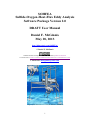
1
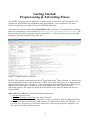
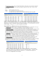
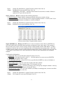
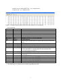
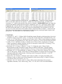
SOHFEA
Sulfide-Oxygen-Heat-Flux Eddy Analysis
Software Package Version 2.0
DRAFT User Manual
Daniel F. McGinnis
May 28, 2013
http://dfmcginnis.com/SOHFEA/
© Daniel F. McGinnis
SOHFEA Software Package, Documentation and Data by Daniel F. McGinnis
is licensed under a Creative Commons Attribution-NonCommercial 4.0 International License.
Contact me: [email protected]
Figure from McGinnis et al. 2011 (R. Schwarz, GEOMAR)
1
Synopsis
The aquatic eddy correlation technique is an exciting new technology for measuring benthic fluxes
that is rapidly gaining in popularity. This increasing popularity fortunately comes with advancing
equipment specifications, especially battery and memory capacity.
With the birth of the aquatic eddy technique over a decade ago, deployments were typically limited
to less than about 24 hours. However, with today’s eddy instrumentation, deploy lengths can
theoretically be in excess of 30 days with sampling rates of 64 Hz. This has lead to much longer and
larger data sets; dramatically increasing data handling requirements.
The sheer volume of data produced by the eddy correlation can be intimidating, especially for
newcomers to the field. While most deployments these days seem to be between 3-5 days long, this
still produces over 16 million lines of data that must be processed for quality control and data
analyses in an efficient and expedient manner.
The purpose of the SOHFEA software package is to provide the eddy correlation community with a
fast and efficient means to both preprocessing, averaging and analyzing their eddy flux data.
SOHFEA is designed for both rapid “field-processing” of data for a first look on data quality and
fluxes as well as for final processing for publication-level results.
SOHFEA is written in Fortran 90 and uses a Fortran digital compiler to ensure fast program
execution times (minutes for a 5-day long data set). SOHFEA is free to the academic and scientific
community and can be downloaded at http://dfmcginnis.com/SOHFEA/.
This instruction manual assumes an introductory knowledge of the eddy correlation technique;
however some key references are provided. The manual is geared towards (but not limited to) the
GEOMAR eddy configuration (McGinnis et al. 2011) and the recommended eddy data collection
settings: continuous mode (as opposed to burst) at 64 Hz. In my opinion, these settings provide
optimum flexibility for extracting high quality data.
Please send any comments, feedback, suggestions or bug-reports to [email protected] – I
would be happy to hear from you.
Acknowledgements
I would like to express my thanks to Karl Attard and Kasper Hancke (University of Southern
Denmark) and Andreas Lorke (Uni. Landau – Koblenz) for providing excellent feedback on
SOHFEA and the manual and website.
2
Software Package Overview
SOHFEA Ver. 2.0 consists of three processing categories
- Preprocessing routings containing 3 programs
- Eddy flux program, SOHFEA
- Postprocessing and ancillary routines
1. Preprocessing
The preprocessing routine contains three programs to be run sequentially. These three programs are
run separately so the user has the opportunity to inspect the output after each step to ensure the
results are meeting expectations or to adjust filtering/output parameters. If the user wishes, these
programs can be run sequentially by creating a BATCH program (downloadable on the website).
The programs consist of:
Step1_filter.exe – this program averages the data down, while flagging and removing low-quality
(user-defined) data.
Step2_despike.exe – the next program replaces data flagged in Step1 and despikes the velocity and
O2 data.
Step3_rotate.exe – the final preprocessing program performs a simple double-rotation of the data
to minimize the average vertical velocity and converts the ADV velocity data from instrument
coordinates to earth coordinates.
To run the programs: Simply place your data in the same folder with the programs, fill out
the configuration file, and then execute the programs sequentially.
2. SOHFEA
SOHFEA.exe (and SOHFEAHeat.exe) extracts and outputs the eddy fluxes. In addition, the
program computes the average measured parameters and several other variables of interest.
SOHFEA.exe is used for standard O2 or H2S fluxes (and in principle other constituents).
SOHFEAHeat.exe extracts heat fluxes and is uses the same configuration file.
All software is programmed with Digital Fortran 90 and compiled with global optimizations. The
software is designed for Windows XP, but should operate on any Windows based system. It has not
been tested for other operating systems.
3
Getting Started:
Preprocessing & Extracting Fluxes
The SOHFEA preprocessing is designed to read the Nortek Vector ADV ASCII output file. The
program can be modified to accommodate other input formats – please contact me. An input
conversion program is available to convert UNISENSE Eddy data.
All routines use the same input file ConfigSOHFEA.dat (see below). The program relevant input
blocks are separated by a row of numbers (1234567890123456789x12345678901234567890). The
first 20 spaces are the line input description (up until the ‘x’). The next 20 spaces are for the input
parameters. The line comments begin after the ‘!’.
Figure 1. Example input for SOHFEA
RULES: The program reads input from the 24th space until the 44th space (after the ‘x’ until the end
of the numbering). Please do not include any ‘TABS’ in this field, only spaces. It is suggested that
input be started on the line 1 after the ‘x’. User comments may be added anywhere to the left of the
numbered field (44th space). Each block between the number lines is for each consecutive
processing program. The output file names from one block are the input file names for the next
program block.
Step1_filter.exe – Block 1: Performs the following functions:
1. Averages the input data
2. Applies calibration coefficients (only linear function)
3. Filters: Removes data flagged as bad before average is performed. Data are flagged based on
user specified signal-to-noise ratio (SNR; default = 5) and beam correlation (BC; default = 70) –
Lines 15 & 16, respectively. If all points removed for a bin average, that bin is assigned a -99.
The -99 will be replaced in the next step.
4
4. Outputs time in hours: Line 14 ‘Start Time (Hours)’ allows the user to specify a start time
other than 0. This is useful when synchronizing the output with more than 1 eddy or other
instruments.
Input:
Output:
ASCII data file from Vector
Averaged data file (user specified name)
Averaged backscatter (BS) data file with individual beam and average BS.
Figure 2. Example output files Step 1. Left – averaged output. VIOL represents the number of
instances in an averaging bin that data exceed the threshold BC or SNR criteria. If all the points are
discarded (e.g. VIOL = 8) then the velocity values are assigned a -99. The PRESSURE is pressure
in dbar. Right – Time (hr), X, Y, Z, and average BS values (dB).
Step2_despike.exe – Block 2: Performs the following functions:
1. Replaces -99 assigned in Step 1 and outputs warning (WARNING_LOG.DAT) if -99’s are
greater than a consecutive time span indicated by ‘Interp. Warning’ (Line 26).
2. Despike time range: User specifies start and end time for despiking algorithms (both velocity
and O2) – Lines 20 and 21. It is important that periods of very noisy data are excluded (e.g.
when the instrument it being deployed or operated out of water). Extremely noisy data (above
the levels commonly measured) may interfere with the despiking algorithms.
3. Despike O2: The user has option of depiking O2 data (use extreme caution) by specifying an
O2 running mean length in seconds (Line 22 – O2 detrend win.) and a standard deviation
multiple (Line 23 – O2 StDev. Multi). Any data point that falls outside the standard deviation
times the multiple will be removed and replaced by the running mean at that point.
3. Despike velocity: Spike removal for X, Y, and Z velocity based on vertical acceleration
threshold (default for Vz = 0.3 m s-2, line 24). Removed spikes are replaced by linear
interpolation of neighboring data, thus it is necessary to solve iteratively over data set. Default
iterations are set to 100 (line 25). See Goring and Nikora, 2002 for more information.
Figure 3. Example output files Step 2. Left – Output after spikes/-99 values replaced.
Two right columns are the running mean for the O2 despiking. Right – warning if more
than X consecutive seconds of data are replaced (X = 1 second in this example, see
Line 26 in ConfigSOHFEA.dat example).
5
Input:
Output:
Output file from Block 1 (input file name it taken from Line 4).
Despiked file (user specified name Line 19)
WARNING_LOG.DAT – warning of more than X consecutive seconds of data are
replaced (X is specified on line 26).
Step3_rotate.exe – Block 3: Performs the following functions:
1. Double Rotation: Simple double rotation to minimize the mean vertical velocity.
2. Earth Coordinates: User can enter the ADV compass heading from the *.sen file (Line 30) to
rotate the data from instrument coordinates to earth coordinates.
Input:
Output:
Output file from Block 2 (input file name it taken from Line 19).
Rotated file (user specified name Line 29)
Figure 4. Example output files Step 3. ZROT is the
vertical velocity after a simple double rotation.
Step4: SOHFEA.exe – Block 4: SOHFEA.exe is now executed to extract fluxes. SOHFEA.exe
will work with both O2 and H2S data (and other constituents in the same range). The extracted
fluxes in this case use the vertical velocity with the simple double rotation from Block 3. If other
rotations are desired, the user must implement this as an independent step and produce a file with
readable format (simply comma or space delimited with no more than 1 header at the top of the file
– see Figure 4). See Lorke et al. 2012; Wilczak et al. 2001 for more information on coordinate
rotation.
Configuration information:
1. Output file: The user specifies the output file name (Line 32)
2. Frequency of the data in the file (Line 33 – I left this option in so users can run SOHFEA
without going through the first 3 steps).
3. The start and end times: (Lines 34 & 35) are specified for SOHFEA to solve (0 defaults at
start/end of file, respectively).
4. Flux window size: (Line 36) is the time length of the flux window.
5. Channel: (line 37) is either analog output 1 or 2 from the Vector
6. Rotated vertical velocity, z: (Line 38) selecting 1 here will specify using the rotated z velocity,
0 will use the unrotated z velocity for solving the fluxes.
7. Running mean length: (line 39) Time window (seconds) for running mean, can not exceed the
value from the flux window (Line 36).
Input:
Output:
Output file from Block 3 (input file name it taken from Line 29).
Flux output file (user specified name Line 32)
6
cumflux.out & cumfluxSHIFT.out – see example below
Cospectra.out – see example below
Figure 5. Example output SOHFEA.dat. See Table SOHFEA for description.
Table SOHFEA
Time
hours
X-VEL
cm s-1
Y-VEL
cm s-1
Z-VEL
cm s-1
Z-STD
cm s-1
MAG
cm s-1
MAG-STD
cm s-1
DIR
degrees
O2
umol L-1
X or East velocity
Y or North velocity
Vertical velocity
Standard deviation of vertical velocity
Velocity magnitude (only X and Y)
Standard deviation of velocity magnitude
Current direction
Mean oxygen concentration over eddy window (60 seconds in this
case)
-1
O2-STD
umol L
Standard deviation of vertical velocity
-2 -1
FLUX-L
mmol m d
Flux with linear detrending+
FLUX-R
mmol m-2 d-1 Flux with running mean detrending+
LINMIN
mmol m-2 d-1 Linear detrending, time shift. The program shifts to O2 data back
in time (maximum -2 seconds) and seeks the minimum flux
(maximum respiration/uptake)*
RUNMIN
mmol m-2 d-1 Same as LINMIN, but with running mean detrending
LINMAX
mmol m-2 d-1 Same as LINMIN, but seeks maximum flux (in the case of O2
production)
-2 -1
RUNMAX
mmol m d
Same as LINMAX, but with running mean detrending
SLMIN
seconds
Time shift corresponding to LINMIN
SRMIN
seconds
Time shift corresponding to RUNMIN
SLMAX
seconds
Time shift corresponding to LINMAX
SRMAX
seconds
Time shift corresponding to RUNMAX
+ See Moncrieff et al. 2004 for details on detrending methods.
* See McGinnis et al. 2008 for more details regarding time shift.
7
Figure 6. Example output files SOHFEA.exe. Left cumflux.out – CUMFLUX is the cumulative
flux over the entire data series in mmol m-2, which is the time integrated flux. COVAR is the
covariance z´C´, which is the product of the last two columns. cumfluxSHIFT.out is the same but
with the data shifted seeking the most negative (minimum) value over a particular window. Right
Cospectra.out – this file provides an estimate for the cumulative cospectra (unshifted data) after
the method from McGinnis et al. 2008. The left most column FREQ is the frequency in Hz. The
very top row is the mean time of the window (hours), and below that in column 2 – onward are the
fluxes associated with a that time and integrated to that frequency (starting at high frequency and
going lower – See McGinnis et al. 2008 for more detail).
CITATIONS
1. Goring, D. G., and V. I. Nikora (2002), Despiking acoustic Doppler velocimeter data, Journal of
Hydraulic Engineering-ASCE, 128(1), 117-126, doi:10.1061/(asce)0733-9429(2002)128:1(117).
2. Lorke, A., D. F. McGinnis, A. Maeck, and H. Fischer (2012), Effect of ship locking on sediment
oxygen uptake in impounded rivers, Water Resources Research, 48, doi:10.1029/2012wr012483.
3. Lorrai, C., D. F. McGinnis, P. Berg, A. Brand, and A. Wüest (2010), Application of Oxygen
Eddy Correlation in Aquatic Systems, Journal of Atmospheric and Oceanic Technology, 27(9),
1533-1546, doi:10.1175/2010jtecho723.1.
4. McGinnis, D. F., P. Berg, A. Brand, C. Lorrai, T. J. Edmonds, and A. Wüest (2008),
Measurements of eddy correlation oxygen fluxes in shallow freshwaters: Towards routine
applications and analysis, Geophysical Research Letters, 35(4), doi:10.1029/2007gl032747.
5. McGinnis, D. F., S. Cherednichenko, S. Sommer, P. Berg, L. Rovelli, R. Schwarz, R. N. Glud,
and P. Linke (2011), Simple, robust eddy correlation amplifier for aquatic dissolved oxygen and
hydrogen sulfide flux measurements, Limnology and Oceanography-Methods, 9, 340-347,
doi:10.4319/lom.2011.9.340.
6. Moncrieff, J., R. Clement, J. Finnigan, and T. Meyers (2004), Averaging, detrending, and
filtering of eddy covariance time series, Handbook of Micrometeorology: a Guide for Surface
Flux Measurement and Analysis, 29, 7-31.
7. Wilczak, J. M., S. P. Oncley, and S. A. Stage (2001), Sonic anemometer tilt correction
algorithms, Boundary-Layer Meteorology, 99(1), 127-150, doi:10.1023/a:1018966204465.
8