Download Third release of the COMPASS Tool Symphony IDE User Manual

Grant Agreement: 287829
Comprehensive Modelling for Advanced Systems of Systems
Third release of the COMPASS Tool
Symphony IDE User Manual
Technical Note Number: D31.3a
Version: 1.0
Date: November 2013
Public Document
http://www.compass-research.eu
D31.3a - Symphony IDE User Manual (Public)
Contributors:
Joey W. Coleman, Aarhus
Anders Kaels Malmos, Aarhus
Luis Diogo Couto, Aarhus
Peter Gorm Larsen, Aarhus
Richard Payne, Newcastle
Simon Foster, York
Uwe Schulze, Bremen
Adalberto Cajueiro, UFPE
Editors:
Joey W. Coleman, AU
Reviewers:
2
D31.3a - Symphony IDE User Manual (Public)
Document History
Ver
0.1
0.2
0.3
0.4
0.5
0.6
0.7
0.8
0.9
0.10
0.11
0.12
0.13
0.14
0.15
0.16
1.0
Date
24-10-2013
26-10-2013
28-10-2013
28-10-2013
30-10-2013
01-11-2013
07-11-2013
07-11-2013
08-11-2013
08-11-2013
11-11-2013
12-11-2013
20-11-2013
26-11-2013
26-11-2013
26-11-2013
27-11-2013
Author
JWC
PGL
JWC
LDC
RJP
US
JWC
US
PGL
ACF
RJP
JWC
AKM
JWC
RJP
SF
JWC
Description
Initial document version
Added information about Symphony
Edits for “Symphony”, editing, consistency, etc
Updates to the POG section
Updates to the TP section
Initial addition of RTT section
Minor edits for consistency
Update the RTT section
Adding concluding remarks
Update Model Checker documentation
Updates to the TP section
Prep for internal review
Update simulator sections
Prep for final version
Update TP section
Update TP support appendix
Final version
3
D31.3a - Symphony IDE User Manual (Public)
Contents
1
Introduction
6
2
Obtaining the Software
8
3
Using the Symphony Perspective
3.1 Eclipse Terminology . . . . . . . . . . . . . . . . . . . . . . . . . .
9
9
4
Managing Symphony Projects
4.1 Creating new Symphony projects . . . . . . . . . . . . .
4.2 Importing Symphony projects . . . . . . . . . . . . . .
4.2.1 COMPASS project Symphony example projects .
4.2.2 Existing Symphony projects . . . . . . . . . . .
4.3 Exporting Symphony projects . . . . . . . . . . . . . .
.
.
.
.
.
11
11
11
11
12
12
5
The CML Type Checker
5.1 Output . . . . . . . . . . . . . . . . . . . . . . . . . . . . . . . . . .
5.2 Representation . . . . . . . . . . . . . . . . . . . . . . . . . . . . .
15
15
15
6
The Symphony Simulator
6.1 Creating a Launch Configuration
6.2 Launch Via Shortcut . . . . . .
6.3 Interpretation . . . . . . . . . .
6.3.1 Animation . . . . . . .
6.3.2 Simulation . . . . . . .
6.3.3 Run/Debug . . . . . . .
6.3.4 Error reporting . . . . .
17
17
19
20
20
21
22
23
.
.
.
.
.
.
.
.
.
.
.
.
.
.
.
.
.
.
.
.
.
.
.
.
.
.
.
.
.
.
.
.
.
.
.
.
.
.
.
.
.
.
.
.
.
.
.
.
.
.
.
.
.
.
.
.
.
.
.
.
.
.
.
.
.
.
.
.
.
.
.
.
.
.
.
.
.
.
.
.
.
.
.
.
.
.
.
.
.
.
.
.
.
.
.
.
.
.
.
.
.
.
.
7
The Symphony Proof Obligation Generator
8
Theorem Proving
8.1 Introduction . . . . . . . . . . . . . . . . . . . . . . . . .
8.2 Obtaining the Software . . . . . . . . . . . . . . . . . . .
8.2.1 Isabelle . . . . . . . . . . . . . . . . . . . . . . .
8.2.2 UTP/CML Theories . . . . . . . . . . . . . . . .
8.3 Configuration Instructions for Isabelle/UTP . . . . . . . .
8.4 Using the Isabelle perspective with the Symphony IDE . .
8.5 Proving CML Theorems . . . . . . . . . . . . . . . . . .
8.5.1 Discharging Proof Obligations . . . . . . . . . . .
8.5.2 Discharging Model-Specific Validation Conjectures
.
.
.
.
.
.
.
.
.
.
.
.
.
.
.
.
.
.
.
.
.
.
.
.
.
.
.
.
.
.
.
.
.
.
.
.
.
.
.
.
.
.
.
.
.
.
.
.
.
.
.
.
.
.
.
.
.
.
.
.
.
.
.
.
.
.
.
25
.
.
.
.
.
.
.
.
.
26
26
26
26
27
28
29
31
31
32
Model Checking
9.1 Installing Auxiliary Software . . . . . . . . . . . . . . . . . . . . . .
9.2 Using the CML model checker . . . . . . . . . . . . . . . . . . . . .
9.3 Examples . . . . . . . . . . . . . . . . . . . . . . . . . . . . . . . .
35
35
35
37
10 Test Generation
10.1 RTT-MBT Perspective . . . . . . . . . . . . . . . . . . . . . . . . .
10.2 Terms and Concepts . . . . . . . . . . . . . . . . . . . . . . . . . . .
10.3 Create a Project . . . . . . . . . . . . . . . . . . . . . . . . . . . . .
40
40
41
43
9
4
.
.
.
.
.
.
.
.
.
.
.
.
.
.
.
.
.
.
.
.
.
.
.
.
.
.
.
.
.
.
.
.
.
.
.
.
.
.
.
.
.
.
.
.
.
D31.3a - Symphony IDE User Manual (Public)
10.4 Automated Generation of the First Test Procedure . . . . . . . . . . .
10.4.1 Configure the first test procedure generation context . . . . .
10.4.2 Check and Edit the Signal Map . . . . . . . . . . . . . . . .
10.4.3 Generate the First Test Procedure . . . . . . . . . . . . . . .
10.5 Creating Further Test Procedures . . . . . . . . . . . . . . . . . . . .
10.6 Test Generation Configuration . . . . . . . . . . . . . . . . . . . . .
10.6.1 Basic Configuration . . . . . . . . . . . . . . . . . . . . . .
10.6.2 Detailed Configuration of Test Procedure Generation Contexts
10.6.3 Advanced Configuration . . . . . . . . . . . . . . . . . . . .
10.6.4 Detailed Configuration of the Signal Map . . . . . . . . . . .
10.7 Test Procedure Generation . . . . . . . . . . . . . . . . . . . . . . .
10.7.1 Activating the Generation Process . . . . . . . . . . . . . . .
10.7.2 Results of Test Procedure Generation – Validation Aspects . .
10.8 Test Procedure Execution . . . . . . . . . . . . . . . . . . . . . . . .
10.8.1 Compile Test Procedure . . . . . . . . . . . . . . . . . . . .
10.8.2 Run Test Procedure . . . . . . . . . . . . . . . . . . . . . . .
10.8.3 Replay Test Result . . . . . . . . . . . . . . . . . . . . . . .
10.8.4 Generate Documentation . . . . . . . . . . . . . . . . . . . .
45
45
46
46
46
47
47
48
51
53
55
55
55
57
58
58
59
59
11 Conclusion
60
A CML Support in the Interpreter
A.1 Actions . . . . . . . . . . . . . . . . . . . . . . . . . . . . . . . . .
A.2 Processes . . . . . . . . . . . . . . . . . . . . . . . . . . . . . . . .
61
62
67
B CML Support in the Theorem Prover
B.1 Actions . . . . . . . . . . . . . .
B.2 Declarations . . . . . . . . . . . .
B.3 Types . . . . . . . . . . . . . . .
B.4 Expressions . . . . . . . . . . . .
B.5 Operations . . . . . . . . . . . . .
.
.
.
.
.
.
.
.
.
.
.
.
.
.
.
.
.
.
.
.
.
.
.
.
.
.
.
.
.
.
.
.
.
.
.
.
.
.
.
.
.
.
.
.
.
.
.
.
.
.
.
.
.
.
.
.
.
.
.
.
.
.
.
.
.
.
.
.
.
.
.
.
.
.
.
.
.
.
.
.
.
.
.
.
.
.
.
.
.
.
.
.
.
.
.
69
70
75
76
76
77
C CML Support in the Model Checker
C.1 Actions . . . . . . . . . . . . .
C.2 Declarations . . . . . . . . . . .
C.3 Types . . . . . . . . . . . . . .
C.4 Operations . . . . . . . . . . . .
.
.
.
.
.
.
.
.
.
.
.
.
.
.
.
.
.
.
.
.
.
.
.
.
.
.
.
.
.
.
.
.
.
.
.
.
.
.
.
.
.
.
.
.
.
.
.
.
.
.
.
.
.
.
.
.
.
.
.
.
.
.
.
.
.
.
.
.
.
.
.
.
.
.
.
.
78
79
84
85
86
.
.
.
.
5
D31.3a - Symphony IDE User Manual (Public)
1
Introduction
This document is a user manual for the Symphony IDE (produced in the COMPASS
project), an open source tool supporting systematic engineering of System of Systems
(SoSs) using the COMPASS Modelling Language (CML). The ultimate target is a tool
that is built on top of the Eclipse platform, that integrates with the RT-Tester tool and
also integrates with Artisan Studio. This document is targeted at users with limited
experience working with Eclipse-based tools. Directions are given as to where to obtain
the software.
This user manual does not provide details regarding the underlying CML formalism.
Thus if you are not familiar with this, we suggest the tutorial for CML before proceeding with this user manual [?, ?]. However, users broadly familiar with CML may find
the Tool Grammar reference (COMPASS Deliverable D31.3c [?]) useful to ensure that
the they are using the exact syntax accepted by the tool.
This version of the document supports version 0.2.4 of the Symphony IDE. The intent is
to introduce readers to how this version of the tool interacts with CML models.
The main tool is the Symphony IDE,1 which integrates all of the available CML analysis functionality and provides editing abilities. The architectural relationship between
Symphony and the rest of the tools used in the COMPASS project is shown in Figure 1.
Figure 1: The COMPASS tools
On the left of Figure 1 is Artisan Studio, which provides the ability to model SoSs
using SysML. It is possible to generate XMI model files and CML files from SysML
models in Artisan Studo, and those are recognised within the Symphony tool. Work in
1 In earlier releases this was called the COMPASS IDE but it has been renamed to create a better branding
for continuation of the product after the completion of the project. It is built on top of the Overture open
source tool suite in the same way as the Crescendo tool (originally developed in the DESTECS project). This
series of tools has names with a musical theme, and are found online at the URLs: www.overturetool.
org, www.crescendotool.org and www.symphonytool.org.
6
D31.3a - Symphony IDE User Manual (Public)
project Task 3.3.3 on static fault analysis is using the external HipHops tool to analyse
models in Artisan Studio.
In the centre of Figure 1 is the main Symphony tool itself, with many of its submodules identified, and the larger grey boxes correspond to specific plugins. In particular,
the Symphony IDE’s connection to the external RT-Tester tool facilitates the use of
automated test generation techniques on SoS models, and the Symphony IDE acts as a
control console for the RT-Tester platform. There are also dependencies on the Isabelle
theorem prover by the theorem prover plugin, and on the Microsoft FORMULA model
checker by the model checker plugin.
Section 2 describes how to obtain the software and install it on your own computer.
Section 3 explains the different views in the Symphony Eclipse perspective. This is
followed by Section 4 which explains how to manage different projects in the Symphony IDE. Section 5 describes what output the CML typechecker will produce, and
where it may be found in the Symphony IDE.
For the situation where a user wishes to simulate a CML model, Section 6 describes
the interface to the CML simulator as included in the Symphony IDE.
Section 7 describes how to access the output from the proof obligation generator, which
can be linked to the theorem prover as described in Section 8. CML models may also
be model checked through use of the model checking plugin described in Section 9.
CML models can also be used to drive test generation through the RT-Tester plugin,
as described in Section 10. Finally, Section 11 provides a few concluding remarks
and look ahead for the future development in the remaining period of the COMPASS
project.
7
D31.3a - Symphony IDE User Manual (Public)
2
Obtaining the Software
This section explains how to obtain the Symphony IDE, described in this user manual.
The Symphony tool suite is an open source tool, developed by the universities and industrial partners involved in the COMPASS EU-FP7 project [?]. The tool is developed
on top of the Eclipse platform.2
The source code and pre-built releases for the Symphony IDE are hosted on SourceForge.net, as this has been selected as our primary mechanism for supporting the community of users of CML and the developers building tools for the Symphony platform.
It has facilities for file distribution, source code hosting, and bug reporting.
The simplest way to run the Symphony IDE is to download it from the SourceForge.net
project files download page at
https://sf.net/p/compassresearch/files/Releases/0.2.4/
This download is a specially-built version of the Eclipse platform that only includes
the components that are neccessary to run the Symphony IDE— it does not include the
Java development tools usually associated with the Eclipse platform.
Once the tool has been downloaded, in order to run it, simply unzip the archive into the
directory of your choice and run the Symphony executable. The tool is self-contained
so no further installation is necessary.
The Symphony IDE requires the Java SE Runtime Environment (JRE) version 7 or
later. On Windows environments, either the 32-bit or 64-bit versions may be used, on
Mac OS X and Linux, the 64-bit version is required.
Artisan Studio and the RT-Tester environment are available from Atego and Verified
Systems International, respectively, and are not distributed through the SourceForge.net
website. Obtaining those software environments is outside of the scope of this document.
2 http://www.eclipse.org
8
D31.3a - Symphony IDE User Manual (Public)
3
Using the Symphony Perspective
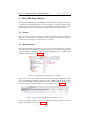
When the Symphony IDE is started, the splash screen from Figure 2 should appear.
The first time it is started you must decide where you want the default place for your
projects to be. Click ok to start using the default workspace and close the welcome
screen to get started for the first time.
Figure 2: The Symphony spash screen used at startup
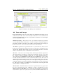
3.1
Eclipse Terminology
Eclipse is an open source platform based around a workbench that provides a common
look and feel to a large collection of extension products. Thus, for a user familiar with
one Eclipse product it will generally be easy to start using a different product on the
same workbench. The Eclipse workbench consists of several panels known as views,
such as the Symphony Explorer view at the top left of Figure 3. A collection of panels
is called a perspective, for example Figure 3 shows the standard Symphony perspective.
This consists of a set of views for managing Symphony projects and viewing and editing files in a project. Different perspectives are available in the Symphony IDE as will
be described later, but for the moment think of a perspective as a useful composition of
views for conducting a particular task.
The Symphony Explorer view lets you create, select, and delete Symphony projects
and navigate between the files in these projects, as well as adding new files to existing
projects.
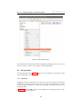
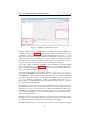
The Outline view, on the right hand side of Figure 3, presents an outline of the file
selected in the editor. This view displays any declared CML definitions such as their
state components, values, types, functions, operations and processes.3 The type of the
definitions are also shown in the outline view. The Outline view is at the moment only
available for the CML models of the system. In the case another type of file is selected,
the message An outline is not available will be displayed.
The outline will have an appropriate structure based on the type of CML construct
found in the source file that is displayed in the visible CML editor. In Figure 4 a CML
3 In
a later version of the tool the outline view will also support other types of files.
9
D31.3a - Symphony IDE User Manual (Public)
CML Editor
Outline View
Symphony
Explorer
Problem View
Figure 3: Outline of the Symphony Workbench.
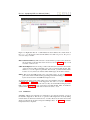
Figure 4: The outline view showing CML class named Component1 on the left. On the
right the outline view is showing a CML process and its actions.
class is outlined on the left reflecting the structure of a class. On the right Figure 4
depicts a CML process and lists its actions. In the current version of the Symphony
IDE, outline decorations are omitted but are planned to be as follows: The icon in
front of a name indicates the type of respective CML element: a brown circle with a
“V” indicates a value, a purple circle with a “T” indicates a Type, a red circle with
a “P” indicates a process, a blue circle with an “O” indicates an operation, a yellow
circle with a “F” indicates a function, a green circle with a “C” indicates a class, a dark
brown circle with “Cs” indicates a chanset and a light brown circle with “Ch” indicates
a channel.
The higher level elements of the outline begin collapsed and can be expanded to show
their child nodes. For example, a process can be expanded in order to see its actions,
operations, and so forth.
Clicking on the name of a definition will move the cursor in the editor to the definition.
The outline will also automatically highlight whichever node corresponds to the cursor
position as it changes.
10
D31.3a - Symphony IDE User Manual (Public)
4
Managing Symphony Projects
This section explains how to use the tool to manage Symphony projects. Step by step
instructions for importing, exporting and creating projects will be given.
4.1
Creating new Symphony projects
Follow these steps in order to create a new Symphony project:
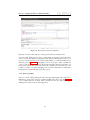
1. Create a new project by choosing File → New → Project → Symphony project
(see Figure 5)
2. Type in a project name (see Figure 6)
3. Click the button Finish.
Figure 5: Create Project Wizard
4.2
Importing Symphony projects
4.2.1
COMPASS project Symphony example projects
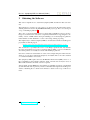
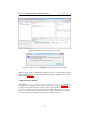
The Symphony IDE comes bundled with a package of examples that users may experiement with. To import them into the the workspace, use the following procedure:
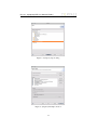
1. Right-click the explorer view and select Import, then choose Symphony → Symphony Examples. See Figure 7 for more details. Click Next to proceed.
2. The available example projects will be presented in the next dialog, as shown
in Figure 8. Choose the desired examples, then click Finish and they will be
automatically imported into your workspace.
11
D31.3a - Symphony IDE User Manual (Public)
Figure 6: Create Project Wizard
4.2.2
Existing Symphony projects
Follow these steps in order to import an already existing Symphony project:
1. Right-click the explorer view and select Import, followed by General → Existing
Projects into Workspace; this can be seen in Figure 7. Click Next to proceed.
2. If the project is contained in a folder, select the radio button Select root directory,
if it is contained in a compressed file select Select archive file. These options will
be presented in a dialog similar to that in Figure 8.
3. Click on the active Browse button and navigate in the file system until the project
to be imported is located.
4. Click the button Finish. The imported project will appear on the Symphony explorer view.
4.3
Exporting Symphony projects
Follow these steps in order to export a Symphony project:
1. Right click on the target project and select Export, followed by General →
Archive File. See Figure 9 for more details.
2. A new window like the one shown in Figure 10 will follow. In this case the
selected project will appear as root node on the left side of it. It is possible
to browse through the contents of the project and select the correct files to be
exported. All the files contained in the project will be selected by default.
3. Enter a name for the archive file in the text box following To archive file. A
specific path to place the final file can be selected through the button Browse.
4. Click on the Finish button to complete the export process.
12
D31.3a - Symphony IDE User Manual (Public)
Figure 7: Symphony import dialog
Figure 8: Symphony Example selection
13
D31.3a - Symphony IDE User Manual (Public)
Figure 9: Select an output format for the exporting process.
Figure 10: Project ready to be exported.
14
D31.3a - Symphony IDE User Manual (Public)
5
The CML Type Checker
The Symphony IDE ships with the CML Type Checker. The Type Checker checks type
consistentcy and referential integrity of your model. Type consistentcy includes checking that operator and variable types are respected. Referential integrity includes checking that named references exists and have an appropriate type for their context.
5.1
Output
The type checker produces two kinds of artifacts: Type Errors and Type Warnings.
Both carry a reference to the offending bit of the model, a description of what is ill
formed and an exact location of where the issue occurred.
5.2
Representation
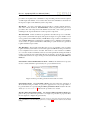
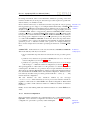
In the Symphony IDE user interface type errors show up in three places. To point the
user at the exact piece of CML-source causing an error, an error marker will be showing
in the left margin of its Editor. Additionally, the problematic piece of syntax will be
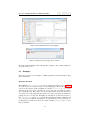
underlined with red as seen in Figure 11.
Figure 11: User Interface showing type error markers.
Type errors are also made visible in the user interface through the CML Project Explorer. The CML Project Explorer offers a tree view of CML model file structure. If an
error occurs in a CML-source file then all of folders containing that file up through the
hierarchy to the project level will have a red error marker (also see Figure 11).
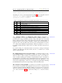
Figure 12: User Interface problems view with type errors.
To give the complete picture for all errors in a given model the problem view shows
the list of all generated errors (see Figure 12).
15
D31.3a - Symphony IDE User Manual (Public)
Type error markers will be updated whenever a CML-Source file is saved with changes.
To force a re-check of all source files again click the Project → Clean . . . item from
the menu bar.
One last thing to notice is that the Outline view, when displayed, is only updated for
source-files that parse correctly. Thus, files that have parse errors will not have their
Outline view updated and may also contain type errors. Seeing an outline is only an
indication the model is syntactically correct.
16
D31.3a - Symphony IDE User Manual (Public)
6
The Symphony Simulator
This chatper explains how to simulate/animate a CML model with the Symphony IDE.
This includes how to add and configure launch configurations, and how the interpreter
is launched and used.
First, the basic modes of operation are explained. The interpreter operates in two
modes, Run and Debug, and within these modes there are three options Animate, Simulate and Remote Control. These options control the level of user interaction and are
described below:
1. Simulate: This option will interpret the model without any user interaction.
When faced with a choice of several observable events, one will be chosen in
a random but deterministic manner. Thus, the simulation will always make the
same choices for every run of the same model. This behavior is implemented
by the use of a pseudo-random number generator that has been initialised with
a constant seed. This random number generator is used to resolve the choice
between events, and will produce the same series of actions when presented with
the same series of choices.
2. Animate: This option will interpret the model with user interaction. All observable events are selected by the user.
3. Remote Control: This option enables the interpreter to be remote controlled by
an external Java class implementing the IRemoteControl interface and located in
the “lib” folder of the project.
The modes of operation controls the interpreter’s behaviour with respect to breakpoints:
1. Run: This will simulate/animate the model ignoring any breakpoints.
2. Debug: This will simulate/animate the model and suspend execution at all enabled breakpoints.
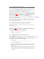
6.1
Creating a Launch Configuration
To create a launch configuration, you first click on the small arrow next to either the
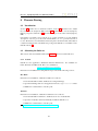
debug button or the run button (depending on the desired mode) as shown in Figure 13.
Once clicked, a drop-down menu will appear with either Debug configurations or Run
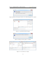
configurations (depending on which button you clicked); select the appropriate configurations option. This will open a configurations dialog like the one shown in Figure 14.
All of the existing CML launch configurations will appear under CML Model. To create a new launch configuration you may double-click on CML Model or on the New
launch configuration button, then an empty launch configuration will appear as shown
in Figure 14 with the name New Configuration (possibly followed by a number if this
name is already used). To edit an existing configuration, click on the desired launch
configuration name and the details will appear on the right side of the dialogue.
As seen in Figure 14 a project name and a process name need to be associated with a
launch configuration along with the mode of operation as discussed in Section 6. When
17
D31.3a - Symphony IDE User Manual (Public)
Figure 13: Screenshot of the toolbar of the Symphony IDE showing the debug button
(left) and run button (right) highlighted.
Figure 14: The launch configuration dialog showing a newly created launch configuration
choosing a project, you can either write the name or click on the Browse button which
shows a list of all the available projects and choose one from there. The selection of
the process name is identical.
The selected project must exist in the workspace, and the process named must exist
within it. It will not be possible to launch if they do not. In the left corner of Figure 14
a small red icon with an “X” and a message will indicate what is wrong. In the figure
it indicates that no project has been set, so this should be the first thing to do.
18
D31.3a - Symphony IDE User Manual (Public)
After setting the project name and process name, the Apply button must be clicked to
save the changes to the launch configuration. If the project exists, is open and a process
with the specified name exists in the project, then the Run or Debug button will be
active and it is possible to launch the simulation as shown in Figure 15. Furthermore,
the decision of whether to animate, simulate or remote control the model is decided by
the radio buttons in the Execution Mode groupbox in the buttom, the default setting is
to animate.
Figure 15: The configuration dialog after a project and process has been selected
This launch configuration will now appear in the drop-down menu as described at the
beginning of this section. The actual interpretation will be described in Section 6.3.
6.2
Launch Via Shortcut
Another way to launch a simulation is through a shortcut in the Symphony explorer
view in the CML perspective. To access this, right click on a cml file to make the
context menu appear. From here either choose Debug As → CML Model or Run As →
CML Model as depicted in Figure 16.
After that, two things can happen: if the CML source file only contains one process
then this process will be launched. If however, more than one process is defined, then
a process selection dialog appears with a list of possible processes. This is shown in
Figure 17.
To launch a simulation, a process must be chosen. This is done by double-clicking one
of the process names in the list, or selecting it and pressing ”OK”. This will launch a
simulation with that process as the top-level process.
19
D31.3a - Symphony IDE User Manual (Public)
Figure 16: The quick launcher
If you launch via a shortcut then a launch configuration named Quick Launch (or Quick
Launch(<number>) if more exist) will be created and launched.
6.3
Interpretation
As mentioned at the start of Section 6, there are four possible ways to interpret a model,
each of them will be described.
6.3.1
Animation
Animating a model is achieved by choosing the Animate radio button in the launch
configuration as described in the last section, this is also the default behavior. In this
mode of operation the user has to pick every observable event before they can occur
through the GUI.
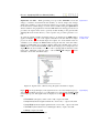
In Figure 18 a small CML model is being animated in the debug perspective. The
following windows are depicted:
20
D31.3a - Symphony IDE User Manual (Public)
Figure 17: Right after Run As → CML Model has been clicked, the context menu of
the test.cml file appears. Since the file defines more than one process, the process
selection dialog is shown.
Observable Event History This window is located in the top right corner and shows
the observable events that have been selected so far. In Figure 18 only a tock
event has occurred so far.
CML Event Options This shows the possible events that can occur in the current state
of the model. To make a particular event occur you must double-click it. Furthermore, to see the origin of a particular offered event, you must click it and the
location of every involved construct will be marked gray in the editor window.
Editor This shows the CML model source code with a twist. As seen in Figure 18
parts of the model is marked with a gray background. This marking is determined
by the selected event in the CML Event Options view.
To understand how the views work together a two-step animation is shown in Figure 18
and Figure 19. In Figure 18 tock has happened once and a tock event is currently
selected. Since process A and B both offer tock they are both marked with gray in the
Editor view. In Figure 19 the init event has been double-clicked. Thus, A and B has
synchronized on init and they both wait for the next event to occur.
6.3.2
Simulation
Simulating without user interaction is achieved by choosing the Simulate option in
the launch configuration. This mode of operation will interpret the model by taking
random decisions when faced with a choice of events. However, the same choices will
always be taken if the model is interpreted multiple times. In Figure 20 a simulate
interpretation has completed.
21
D31.3a - Symphony IDE User Manual (Public)
Figure 18: A CML model animated in the debug perspective.
Figure 19: The init event has just occurred and it is now currently offering a, b and
tock, where a is currently selected
6.3.3
Run/Debug
In addition to the two modes of operation Animate and Simulate the standard modes
Run and Debug also exist. The Run mode will interpret the model without ever breaking
on any breakpoints. The Debug however will stop on any enabled breakpoint in the
model.
When a Debug configuration is launched the perspective changes to the Eclipse Debug
22
D31.3a - Symphony IDE User Manual (Public)
Figure 20: The model has just been simulated
Perspective, however Run will stay on the perspective that is currently active.
To create a new breakpoint you have to double-click on the ruler to left in the editor
view, if created, this will insert a small dot to the left ruler. Breakpoints can be set on
processes, actions and expressions only. Double-clicking on a existing breakpoint dot
will remove it. In Figure 21 a debugging session is in progress. Here, a breakpoint
on the a event in process A has been hit and the interpreter has been suspended. At
this point the current state can be inspected in the variables view. From here it is both
possible to resume or stop the debugging session. If the resume button is clicked the
interpretation is resumed and the stop button stops it.
6.3.4
Error reporting
If an error occurs a dialog will appear with a message explaining the cause of the error.
Furthermore, the location of the error will be marked in the editor view. In Figure 22
a post condition has been violated. This is described in the error dialog and a gray
marking shows where in the model it happened.
23
D31.3a - Symphony IDE User Manual (Public)
Figure 21: The interpreter is currently suspended because a breakpoint is hit. The
line of the breakpoint is highlighted in green and has an arrow in the left ruler. In the
variable view in the top right corner the state variable for process A can be seen.
Figure 22: The interpreter has stopped because a post condition has been violated
24
D31.3a - Symphony IDE User Manual (Public)
7
The Symphony Proof Obligation Generator
Usage of the Symphony Proof Obligation Generator (POG) is quite simple. The POG
has only one function: generating the POs. In order to do this, the user must select
a CML project (or a CML file in said project), right-click and select CML-POG →
Generate Proof Obligations from the context menu. This is shown in Figure 23.
Figure 23: Invoking the Symphony POG.
Once the POG has run successfully, the generated POs are displayed in a view to the
right of the editor (if the default POG perspective is enabled). If you click on any PO
in this list ,and its predicate can be seen in a frame below the PO list. This is shown in
Figure 24.
Finally, any PO can be double-clicked and the editor will highlight the relevant portion
of the CML model that yielded that PO.
Figure 24: Results of proof obligation generation
25
D31.3a - Symphony IDE User Manual (Public)
8
Theorem Proving
8.1
Introduction
Section 8.2 describes how to obtain the software. Section 8.3 describes how to install
the software in the Symphony IDE, Section 8.4 explains how to use the Symphony
Eclipse perspective and Section 8.5 describes how to prove theorems in the Symphony
IDE.
It should be noted that it is beyond the scope of this document to provide detailed
descriptions of how to prove theorems in the Isabelle tool, or to provide a tutorial on
it’s use. We therefore recommend that interested parties should read this deliverable in
conjunction with tutorials on Isabelle and proving in the Isabelle tool, available on the
Isabelle website.4
8.2
Obtaining the Software
This section of the user manual assumes that Section 2 has been read and followed.
8.2.1
Isabelle
Isabelle is a free application, distributed under the BSD license. It is available for
Linux, Windows and Mac OS X. The tool is available at:
http://isabelle.in.tum.de
Instructions for installation for each platform are provided in the following sections:
Mac OS X
Instructions for installation of Isabelle for Mac are as follows:
1. Download Isabelle for Mac, distributed as a dmg disk image.
2. Open the disk image and move the application into the /Applications folder.
3. NOTE: Do not launch the tool at this point.
Windows
Instructions for installation of Isabelle for Windows are as follows:
1. Download Isabelle for Windows, distributed as an exe executable file.
2. Open the executable, which automatically installs the Isabelle tool.
3. NOTE: Do not launch the tool at this point.
4 http://isabelle.in.tum.de/documentation.html
26
D31.3a - Symphony IDE User Manual (Public)
Linux
Instructions for installation of Isabelle for Linux are as follows:
1. Download Isabelle for Linux, distributed as a tar bundled archive.
2. Unpack the archive into the suggested target directory.
3. NOTE: Do not launch the tool at this point.
8.2.2
UTP/CML Theories
To prove theorems and lemmas for CML models, Isabelle must have access to the
UTP and CML Theories. Instructions for obtaining these theories are given below for
different platforms:
Linux, Mac OS X
1. Download the latest version of the utp-isabelle-x archive from
https://sf.net/p/compassresearch/files/HOL-UTP-CML/
Linux/Mac can choose either .zip or .tar.bz2.
2. Extract the downloaded theory package and save the utp-isabelle directory to
your machine (e.g. /home/me/Isabelle/utp-isabelle-0.x).
As the CML and UTP theories are improved, new versions will be made available.
As new versions are uploaded, follow the above steps to obtain and unpack the updates.
Windows
1. Download the latest version of the utp-isabelle-x-windows.zip archive
from
https://sf.net/p/compassresearch/files/HOL-UTP-CML/
2. Extract the downloaded theory package.
3. Copy the ROOTS file from the extracted folder to the Isabelle2013 application
folder (e.g. C:\ProgramFiles\Isabelle2013\). Windows will warn
you a ROOTS file already exists. This is ok — choose to replace the existing file.
4. Copy the utp-isabelle folder from the extracted folder to the src folder in
the Isabelle2013 application folder
(e.g. C:\ProgramFiles\Isabelle2013\src\).
As the CML and UTP theories are improved, new versions will be made available.
As new versions are uploaded, follow the above steps to obtain and unpack the updates.
27
D31.3a - Symphony IDE User Manual (Public)
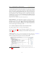
8.3
Configuration Instructions for Isabelle/UTP
This section provides, the steps required to use Isabelle in the Symphony IDE. This
setup procedure is only required on the first use of the theorem prover. However, if a
new version of Symphony is installed, then the procedure must be repeated. Instructions for installation with the Symphony IDE are given below:
1. Open the Symphony IDE.
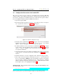
2. From the menu bar, select Theorem Prover → Setup Theorem Prover Configuration. A preferences window, as in Figure 25, will appear.
Figure 25: Isabelle configuration setup
3. In the first text box (labelled a in Figure 25), supply to the location of the Isabelle
application (for example /Applications/Isabelle2013.app). Use the
‘Browse...’ button to navigate to the correct location if required.
4. For Mac and Linux, in the second text box (labelled b in Figure 25), navigate
to the location of the utp-isabelle folder extracted in Section 8.2.2. Use the
‘Browse...’ button to navigate to the correct location if required. This step is
not required for Windows.
5. At present, the theorem prover plugin for Symphony may only be used for noncommercial use. If relevant, the check box (labelled c in Figure 25) must be
checked.
6. Click the Ok button to save the configuration and to finish the setup procedure.
7. Once setup, from the menu bar, select Theorem Prover → Launch Theorem
Prover to run Isabelle. NOTE: the first time Isabelle is invoked, several minutes are needed to initialise and build the theories. Subsequent uses of Isabelle
will not require this long wait. To monitor progress, click on the button on the
bottom right of the tool, as highlighted in Figure 26.
Troubleshooting More detailed instructions are provided at the Isabelle/Eclipse website, which may be of use:
http:
//andriusvelykis.github.io/isabelle-eclipse/getting-started/
If errors persist, please report them using the Symphony bug tracking facility:
28
D31.3a - Symphony IDE User Manual (Public)
Figure 26: Isabelle configuration in Symphony— initialisation progress.
http://sf.net/p/compassresearch/tickets/
8.4
Using the Isabelle perspective with the Symphony IDE
The steps in this section should be followed to begin proving theorems using the Isabelle theorem proving support plugin for the Symphony IDE. The steps enable the
user to prove theorems for a specific CML model.
1. If Isabelle is not already running, from the menu bar, select Theorem Prover
→ Launch Theorem Prover. This will run the Isabelle configuration (defined in
Section 8.3). If there is already an instance of Isabelle running, an error message
will appear, as in Figure 27. This can be safely dismissed.
Figure 27: Overview of Isabelle perspective in Symphony
2. When proving in the Symphony IDE, the Isabelle perspective is used. To open
the perspective manually, select the icon labelled a in Figure 28, and then select
Isabelle and then ok. If the perspective has been used previously, then select the
Isabelle perspective using the button labelled b in Figure 28.
3. Once open, the Isabelle perspective will look like Figure 29. There are various
panes in the perspective as follows:
Project Explorer Similar to the CML perspective — this pane shows the projects
created in the user’s workspace, and their contents.
Theory File Editor A text editor which enables the user to interact with the
theory script and prove theorems, add additional definitions, lemmas and
theorems.
Theory Outline This pane provides an outline to the contents of the selected
29
D31.3a - Symphony IDE User Manual (Public)
Figure 28: Running Isabelle and selecting Isabelle perspective
Figure 29: Overview of Isabelle perspective in Symphony
theory file including definitions, functions, lemmas and theorems and may
be used to navigate the theory file.
Prover Progress A collection of status bars for the currently open theory files
— shows the progress made by Isabelle in proving the scripts in the theory
file.
Prover Output A window to report error messages and the status of the goals
of selected theorems.
Symbol Viewer A quick method of adding mathematical symbols to a theory
file. The user can double-click a symbol which will be added to the proof
script.
4. Using the theory file editor pane, theorems and lemmas may be defined and
proven. The theory editor of Isabelle/Eclipse provides an interactive, asyn-
30
D31.3a - Symphony IDE User Manual (Public)
chronous method for theorem proving, similar to the jEdit interface distributed
with Isabelle. The theory file is submitted to Isabelle and results are reported
asynchronously in the editor and prover output panes. The editor has syntax
highlighting for the Isabelle syntax5 and problems are marked and displayed in
the output pane.
In the next section, we use the steps defined here to use the Isabelle perspective to prove
lemmas related to an example CML model.
8.5
Proving CML Theorems
In this section, we provide a brief overview to theorem proving in the Symphony IDE.
As proving theorems about a CML model in Isabelle is performed in much the same
way as normal theorem proving in Isabelle, the interest reader should refer to tutorials
on theorem proving with Isabelle for more details. We consider two main methods of
theorem proving in the Symphony IDE; discharging POs and model-specific conjectures. In Section 8.5.1, we describe the initial POG-TP link and in Section 8.5.2 we
consider general theorem proving in CML.
8.5.1
Discharging Proof Obligations
Once POs have been generated using the Symphony IDE (see Section 7), the user may
begin to discharge them with the theorem prover. From the POG perspective, the TP
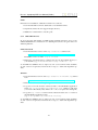
button should be pressed, see Figure 30.
Figure 30: Discharge PO button
This process checks that the CML model is supported by the theorem prover. If there
are any parts of unsupported syntax in the CML model, an error message appears which
informs the user. A list of unsupported syntax is reported in the warning pane of the
Symphony IDE. The individual POs are also checked to ensure they use syntax supported by the theorem prover.
If the model is supported, the theorem prover plugin creates two theory files with the
.thy file extension: a model-specific, read-only, file for the CML model (<modelname>
.thy) and a user-editable file (<modelname>_PO.thy). These files, along with
a read-only version of the CML model, are added to a timestamped folder in the
5 It is beyond the scope of this document to describe the Isabelle syntax – interested readers are directed
to the Isabelle tutorials, as in footnote 4
31
D31.3a - Symphony IDE User Manual (Public)
PROJECT\generated\POG folder of the CML project (see Figure 31). Note —
this file is specific to the current state of the model. Any changes made to the CML
model will not be reflected in the .thy file, and thus the process must be restarted.
The generated model .thy file uses a combination of regular Isabelle syntax and the
Isabelle syntax defined for CML described in more detail in [?].
Figure 31: Project explorer with generated .thy files
In the <modelname>_PO.thy file, each supported PO is represented as an Isabelle
lemma with the proof goal being the PO expression. Each lemma initially uses the “by
(cml auto tac)” proof tactic to attempt to discharge the PO automatically. If this
is not successful, indicated by red error symbols next to a lemma, the user should either
use the keyword oops to skip that PO, or attempt to prove the lemma manually. In the
next section, we introduce the steps for a more manual approach to theorem proving in
the Symphony IDE, including more details on the different thy files generated by the
Symphony theorem prover.
8.5.2
Discharging Model-Specific Validation Conjectures
To illustrate the process of proving model-specific conjectures, we use an example
introduced in Part B of deliverable D33.2 [?] — the Dwarf signal controller.
With a CML model open, right-click on the model filename in the Project Explorer, and
select CML-THY → Generate Theorem Prover THY, as shown in Figure 32.
The CML model is first checked to ensure it is supported by the theorem prover. If
there are any parts of unsupported syntax in the CML model, an error message appears
which informs the user. A list of unsupported syntax is reported in the warning pane of
the Symphony IDE.
If the model is supported, the theorem prover plugin creates two theory files with the
.thy file extension: a model-specific, read-only, file for the CML model (<modelname>
.thy) and a user-editable file (<modelname>_User.thy). These files, along with
a read-only version of the CML model, are added to a timestamped folder in the
PROJECT\generated\Isabelle folder of the CML project (see Figure 31). As
with PO discharging, this file is specific to the current state of the model. Any changes
made to the CML model will not be reflected in the .thy file, and thus the process
must be restarted.
32
D31.3a - Symphony IDE User Manual (Public)
Figure 32: Initiate production of a theory file for a CML model
In Figure 33, the original CML model (Dwarf.cml) and the generated .thy file
(Dwarf.thy) are shown in Symphony. The generated .thy file uses a combination
of regular Isabelle syntax, which is described in various Isabelle manuals and tutorials,
and the Isabelle syntax defined for CML. This Isabelle/CML syntax is described in
detail in [?].
In the corresponding generated timestamped Isabelle directory, a user-editable .thy
file is produced — in this example, that file is named Dwarf_User.thy. This file
imports the utp cml theory and the generated Dwarf model theory. We use the Isabelle
perspective to start stating and proving theorems and lemmas and can begin to prove
some of those theorems introduced in [?]. These theorems, named nsa, molc and fstd,
are added to the user-editable theory file Dwarf_User.thy.
theorems are all simply proved using the cml tac proof tactic. The tactic is applied by
using the line “by (cml tac)” on the line below the theorem. This applies rules and
tactics defined in the isabelle-utp UTP and CML theories imported during the initial
setup of the theorem prover. This tactic is described in more detail in [?].
It is beyond the scope of this document to provide detailed descriptions of theorem
proving, using the Isabelle tool, or to provide a tutorial on it’s use. We therefore recommend that interested parties should read this deliverable in conjunction with tutorials
on Isabelle and proving in the Isabelle tool, available on the Isabelle website.
33
D31.3a - Symphony IDE User Manual (Public)
Figure 33: Example Dwarf CML model and generated .thy file
Figure 34: Discharged theorems in Isabelle perspective
34
D31.3a - Symphony IDE User Manual (Public)
9
Model Checking
The CML model checker is part of the Symphony IDE concerned with support for
analysing models in terms of classical properties (deadlock, livelock and nondeterminism) and, in case of a property is valid, it also provides a useful trace intended provide
detailed information about model’s behaviour.
9.1
Installing Auxiliary Software
The CML model checker is developed over the Microsoft FORMULA tool and GraphViz.
The first is used as the main engine to analyse CML specifications whereas the second
is used to show the counterexample found by the analysis.
The steps to install the CML model checker to work are listed as follows:
1. Download and install the Microsoft FORMULA tool. It is available at
http:
//research.microsoft.com/en-us/um/redmond/projects/formula/
Although the tool is free, it requires Microsoft Visual Studio6 is installed. This
makes the current version of the CML model checker platform dependent as the
underlying framework is from Microsoft.
2. Download and install the GraphViz software. Graphviz is open source graph
visualization software. It allows several kinds of graphs to be written (in a text
file) and graphical output generated in several formats to be presented. GraphViz
is available at http://www.graphviz.org/ and can be installed in several
platforms. The CML model checker uses specifically the dot.exe program,
which provides compilation from a textual description to several formats. We
use the SVG format that is vectorial and accepted by most of Web browsers.
9.2
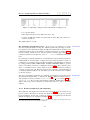
Using the CML model checker
The model checker functionalities are available through the CML Model Checker perspective (see Figure 35), which is composed by the CML Explorer (1), the CML Editor
(2), the Outline view (3), the internal Web browser (to show the counterexample when
invoked) and two further specific views: the CML Model Checker List view (4) to show
the overall result of the analysis and the Model Checker Progress view (5) to show the
execution progress of the analysis.
The analysis of a CML file is invoked through the context menu when the CML or the
MC perspective are active (see Figure 36).
Select the CML file to be analysed. Then, right click the file and select Model check
→ Property to be checked. The option Check MC Compatibility allows a previous
check if the constructs used in the model are supported by the model checker. If some
constructor is not supported by the model checker Symphony shows a warning message (Figure 37) and the user can be more details by accessing the Problems View
(Figure 38).
6 http://www.microsoft.com/visualstudio.
35
D31.3a - Symphony IDE User Manual (Public)
Figure 35: CML Model Checker Perspective
When invoking the analysis, if FORMULA is not installed, the Symphony IDE shows
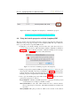
a warning message (see Figure 39). Otherwise, the analysis is performed and the information is shown in different views. The Model Checker list view shows a X or an
X as result of the analysis (meaning satisfiable or unsatisfiable, respectively). For each
analysis performed over a model there is a corresponding line in the Model Checker
List View. If the user edits the model the results of the previous analysis the results of
the previous analysis are still maintained in the Model Checker List View.
It is worth pointing out that if the GraphViz tool is not installed, the Symphony IDE
shows a warning message (see Figure 40). Otherwise, for satisfiable models, the a
graph containing the trace validating the property is accessible by a double clicking the
item on the Model Checker list view.
The model checker analysis uses an auxiliary folder (generated\modelchecker)
to generate the FORMULA file (with extension .4ml). This file is given as input to
the FORMULA tool to be analysed. The graph construction is performed internally
(producing a file with extension .gv) and using the GraphViz software (actually the
dot.exe command) to compile the .gv file to a graph file (with extension .svg).
then Symphony automatically shows the graph file in its internal browser. All these
steps are performed automatically.
The initial state of the graph is two circles; intermediate states are simply circled; and
the deadlocked state (or other special states related to properties verification) has a
different colour (a red tone). Each state has a number and an information (hint) about
the bindings (from variables to values), the name of the owner process, and the current
context (process fragment). To see the internal information of each state just put the
cursor over the state number.
Similarly, transitions are labelled with the corresponding event and also have a hint
showing the source and the target states. This feature is useful to provide information
about which rule (of the structured operational semantics) was applied.
The internal graph builder of the model checker considers the shortest path that makes
36
D31.3a - Symphony IDE User Manual (Public)
Figure 36: The Model Checker Context Menu
Figure 37: Message about unsupported constructs
the analysed file satisfiable. Thus, although there might be other counterexamples, it
shows the shortest one.
9.3
Examples
This section presents some examples of CML specifications and their analysis using
the model checker.
Immediate Deadlock
The CML file action-stop.cml is the most simple deadlock process. Figure 41
shows the result of its analysis and the corresponding graph. The model checker list
view shows the analysis result (satisfiable) for the file action-stop.cml considering the Deadlock property. Trivially, the process has only one initial state that is
also a deadlock state. This can be seen by a double click in the model checker list
view item. It is worth noting that the content of any state of the graph is available by
putting the cursor over the state. Basically, the information of each state has the format (vars,proc), where vars contains the manipulated variables (bindings) and
proc is a process fragment. Furthermore, the generated files can be viewed by refreshing the project. The user can see the content of all files (.4ml,.gv and .svg) as
they are text files.
37
D31.3a - Symphony IDE User Manual (Public)
Figure 38: Details about the unsupported constructs
Figure 39: Messages when FORMULA is invoked but it is not installed
When the analysed file is unsatisfiable, and the user tries to see the graph, the model
checker plugin returns a message indicating that the graph is available only for satisfiable models (Figure 42).
An External Choice Example
The CML file action-externalchoice-nostate2.cml is an example involving the use of auxiliary actions and the external choice operator. Figure 43 shows
its analysis and counterexample to find a deadlock. The external choice [] is translated (via a τ -transition) in the two first transitions (using left association). In state 3,
the process expands (via a τ -transition) the action call C, which leads to an state (4)
from where the transition labelled with c leads to a deadlock state (5).
38
D31.3a - Symphony IDE User Manual (Public)
Figure 40: Messages when graph construction is invoked but GraphViz is not installed
Figure 41: An immediate deadlock example
Figure 42: Message when the graph is not available
Figure 43: An external choice example
39
D31.3a - Symphony IDE User Manual (Public)
10
Test Generation
Introduction
This document describes the RT-Tester Model Based Testing (RTT-MBT) functionality
provided by Symphony using the RT-Tester plugin (RTT-Plugin). The user interface
is explained together with the basic information about model based testing with RTTester. It covers the areas from creating a test project, selecting and using a specific
UML/SysML model to generate test procedures from as well as defining and controlling the test procedure generation process and finally executing and evaluating concrete
test procedures.
Additional information about RTT-MBT can be found in a separate manual [?] that also
describes model based testing with RT-Tester but describes the usage of the RT-Tester
graphical user interface from Verified Systems which is not integrated in Symphony.
Note that in [?], you will find additional chapters about generating test models, defining
test goals, using the model checking capabilities of RTT-MBT as well as different test
strategies and the supported UML and SysML model elements and LTL syntax. These
topics are RTT-MBT specific and independent of the graphical user interfaces. While
this document concentrates on the RTT-Plugin integrated in the COMPASS tool, [?]
and [?] are recommended as side reading to this manual.
The tests that are generated by RTT-Plugin within the COMPASS project are RT-Tester
test procedures. The RT-Tester manual [?] provides detailed information about RTTester and the test language RTTL, the tests are expressed in.
10.1
RTT-MBT Perspective
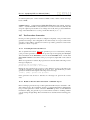
RTT-MBT test generation within Symphony is performed using the RT-Tester perspective (RttPerspective). This perspective is designed to allow model based test generation
and execution of generated test procedures. The perspective shown in figure 44 consists
of a Project Explorer, a Console View, a Progress View, an Outline and a central
area for all Editors. The RTT-MBT Toolbar provides quick access to all RTT-MBT
commands.
The Project Explorer lets you create, select, and delete Symphony projects and navigate between the files in these projects, as well as adding new files to existing projects.
It is a central element of the perspective. RTT-MBT commands normally are performed
on the selected item in the Project Explorer. The icons in the Toolbar are enabled or
disabled with respect to the selected item.
The Console View provides feedback in form of log messages and error messages.
The progress view provides information of the status of the current task. Whenever a
RTT-MBT task is started, a console message is given to indicate the start of the action
an the progress view is reset. The completion of a task is indicated by the progress
bar resting at 100 percent and a message in the console view providing information
whether the task as succeeded (PASS) or not (FAIL).
The Outline is used during the analysis of test procedures. This is explained in detail
in 10.7.2 and [?].
40
D31.3a - Symphony IDE User Manual (Public)
Figure 44: Outline of the RttPerspective Workbench.
10.2
Terms and Concepts
For the understanding of the rest of this chapter, it is vital that the following concepts
are known by the reader. Some of them are just a clarification of how certain terms are
used in this document while others are concepts that are used in the rest of this chapter
and in the RTT-MBT setting.
Model-based testing ”The behaviour of the system under test (SUT) is specified by
a model elaborated in the same style as a model serving for development purposes.
Optionally, the SUT model can be paired with an environment model restricting the
possible interactions of the environment with the SUT.” [Peleska 2013].
Test Model Specifies the expected behaviour of a system under test. This is an important step in model based testing. Note that a test model can be different from a
design model. It might only describe a part of a system under test that is to be tested
and it can describe the system on a different level of abstraction.
Test Case A test case is a set of input values, execution preconditions, expected results and execution postconditions, developed for a particular objective or test condition, such as to exercise a particular program path or to verify compliance with a specific requirement. For RTT-MBT (model based testing with RT-Tester), a test model is
used that describes the behaviour of the system that should be tested. Test cases can
automatically be derived from this model in form of LTL formulas. These test cases
define the precondition and input values, but not the expected outputs, because these
are already defined in the model describing the expected behaviour of the system under
test. The expected outputs are calculated by test oracles that are executed together with
a test procedures covering the test cases.
Test Procedure Detailed instructions for the set-up and execution of a given set of
test cases, and instructions for the evaluation of results of executing the test cases
(RTCA DOI78B). In RTT-MBT, test procedures can automatically be generated from
a test model for a given set of goals (test cases) specified as LTL formulas. These test
41
D31.3a - Symphony IDE User Manual (Public)
procedures are separated into a stimulation component that performs a timed sequence
of SUT inputs and number of test oracles that observe the stimulations and check for
the expected output of the different system components.
Test Oracle A source to determine expected results to compare with the actual result of the software under test. With RTT-MBT, oracles are generated as parts of test
procedures. For each component of the SUT in a test model, a test oracle is generated
checking for the expected behaviour of the respective component.
Test Generation In this document, test generation describes the process of calculating concrete system under test inputs and expected outputs for a given number of test
cases (goals in form of LTL formulas). An RT-Tester test procedure is created that consists of RTTL (RT-Tester test language) specifications for a stimulator and a number
of test oracles. A generic framework for embedding a system under test is generated
together with the test procedure.
Test Execution Test execution describes the process of executing a test procedure
together with the system under test. Note that a generated RT-Tester test procedure has
to be compiled before it can be executed. The result of a test execution is available
as soon as the execution terminates, but test case and requirements tracing information
requires to replay the test result against the test model and to create the test procedure
documentation. These two steps can be performed automatically using RTT-MBT and
RT-Tester.
Generation Context and Execution Context RT-Tester model-based test projects
use two contexts which are represented by two project sub-directories.
Figure 45: Test procedure generation and execution context.
Generation Context. The generation context is the place where the generation of
all model based test procedures of a project is prepared: for every test procedure to
be generated there is a separate test procedure generation context created in the subdirectory TestExecution 7 named as the procedure to be created.
Test Procedure Generation Context. The test procedure generation context is the
place in the project where the generation of a single test procedures is prepared. Here
the test engineers configure the generation by
7 The folder names for the generation context and the execution context can be changed using the Project
page of the RT-Tester section in the Eclipse preferences (see figure 46). The names used here are the default
settings.
42
D31.3a - Symphony IDE User Manual (Public)
• specifying the model portions to be evaluated during the generation,
• specifying the test cases to be covered in the test procedure to be generated.
Execution Context. The execution context is the place where the actual test procedures which can be compiled and executed against the SUT reside in. This context is
contained in directory TestExecution. When RTT-MBT creates a new test procedure based on the information provided in the respective test procedure generation context, the resulting test procedure files are placed in a sub-directory of TestExecution
carrying the same name as the respective generation context . There it can be compiled,
executed, evaluated and documented. The execution context can contain both automatically generated and manually created test procedures. The manual development of test
procedures is described in [?].
Figure 45 shows the test procedure generation context P1 in the generation context
and the respective test procedure P1 in the execution context.
Figure 46: The RTT-MBT General Project Settings Page
10.3
Create a Project
Since RTT-MBT operates in client-server mode, the server name or IP address is required in the RTT-Plugin preferences. Figure 47 shows the Server page of the RTTester section in the Eclipse preferences. In addition to the server name or IP address
and port number, the name and a user identification has to be provided. The RT-Tester
core components, the Test Management System (TMS) and the RTT-MBT test generator are executed on the server. The RTT-MBT project files are created and maintained
on the client side. For every RTT-MBT task that is to be executed, the client synchronises all required files with the server. It is recommended that you use your real
name as the user name and your email address as your user identification. Note that
the user identification has to be unique within the group of users working on the same
RTT-MBT Server. The Server connection can be tested using the main page of the
RT-Tester section in the Eclipse preferences.
RTT-MBT projects used with the RTT-Plugin are generated inside other Symphony
projects. The reason for this is that normally the RTT-MBT test project is a part of a
larger project representing a complete test campaign where several models are used to
generate test procedures for different aspects or parts of a complete system. Every RTTMBT project uses exactly one test model to generate test procedures from. Organising
43
Server name
User name,
user id
D31.3a - Symphony IDE User Manual (Public)
Figure 47: The RTT-MBT Server Settings Page
Figure 48: Creating a new RTT-MBT Project
RTT-MBT projects as folders inside any other type of Eclipse project provides a flexible
way to integrate RTT-MBT projects in your project structure.
Creating an RTT-MBT project is supported by a wizard in the RTT perspective. Select
the Eclipse project in the project explorer and start the wizard using File → New →
Other. In the following dialog, select RTT-MBT Project (Fig. 48) and Next. In the
follwing dialog use the RTT-MBT project name as the folder name for the new Eclipse
component. The wizards creates an empty RTT-MBT project structure below the new
Eclipse component representing the RTT-MBT project.
As stated before, each RTT-MBT project uses exactly one test model. An XMI file
containing your test model has to be imported into the project (see [?] for an explanation how test models are exported to XMI). Typically, this XMI file resides on your
PC where also the test model elaboration took place. Selecting RTT-MBT → Import
Model opens a file browser that can be used to navigate to the directory where your
XMI file (with extension XML or XMI) is located. Select the file and start the im-
44
Model import
D31.3a - Symphony IDE User Manual (Public)
port. As a result of the import, the XMI file is stored as model dump.xml in the
model directory of the RTT-MBT project, together with a LivelockReport.log
file. Please check the livelock report for problems in the model.
After a successful model import a first test generation context P1 has been created in
the generation context (directory TestGeneration) which will be used to generate
the first test procedure along with an initial project configuration and signal map as
explained in Section 10.4. The initial generation context P1 will be used to create
further contexts to be used for the generation of additional test procedures.
If the test model is changed, it can be imported again using the RTT-MBT pull down
menu and selecting Import Model.
Re-importing
test models
Note that re-importing a test model can lead to adjustments in all test procedure generation context definitions and generated test procedures depending on the differences
between the old model and the new one.
10.4
Automated Generation of the First Test Procedure
The automated generation of the very first test procedure is performed in the test procedure generation context
TestGeneration/_P1
which has been created as a result of the model import during project setup, as described in Section 10.3. The configuration of the generation context comprises two
steps, before the automated generation can be activated.
• Configuration of the test procedure generation context.
• Configuration of the signal map.
10.4.1
Configure the first test procedure generation context
The test configuration file contains information about model components to be used
during the generation process and basic test cases to be covered in the test procedure to
be created. Before generating the first procedure P1 it has to be configured by means
of the configuration editor in the RTT-MBT perspective.
• Double-click on
TestGeneration/_P1/conf/configuration.csv
to open the configuration editor.
• Mark the entry in column DEACT (“Deactivate model component during the
generation process”) for every model component that should not be considered
during the generation.
• Mark at least one state machine transition of the SUT in column TC (“Transition
Coverage”). This is a directive to the generator that the model coverage test case
“visit this transition during test execution” will be covered by the test procedure
to be created.
45
Test
configuration
file
D31.3a - Symphony IDE User Manual (Public)
The other columns of the configuration file are explained in more detail in Section 10.6.2.
For the initial generation there is nothing more to do.
10.4.2
Check and Edit the Signal Map
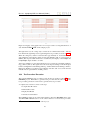
The signal map specifies the input/output direction of each interface signal, as well
as the data ranges admissible for these signals. During project initialisation an initial
version of the signal map is created, based on the type information of the interface
signals specified in the model. The resulting signal map is placed into the test procedure
generation context as file
Signal map
TestGeneration/_P1/conf/signalmap.csv
Since the generator can only guess the appropriate signal ranges and since it may be
useful to change the ranges for specific test purposes it is advisable to open this file by
double-clicking it in the project browser. Then adapt the pre-defined data ranges where
appropriate.
In the turn indication sample project described in [?], for example, the floating point
input voltage has typical value 12V in today’s cars, and the model defines 10 ≤
voltage < 15 as the admissible range. As a consequence, the lower bound 0.0V
and upper bound 16.0V are suitable values to be inserted for voltage in the signal
map.
Adaptations for
the sample
project
Observe that the test data generator will only create inputs to the SUT which are consistent with the data ranges defined in signalmap.csv. This fact may be used to
influence the generation process in the following ways: if an input to the SUT is specified with identical lower and upper bounds in the signal map, the generator will leave
this value constant over the complete test execution time and try to reach the test objectives by manipulating the other inputs only.
Effect of data
ranges on
generator
A more detailed explanation of all columns in the signal map is given in Section 10.6.4.
10.4.3
Generate the First Test Procedure
To generate a test procedure from the initial generation context P1, select the context
P1 in the project browser. Then select RTT-MBT command Generate Test Procedure in the context menu of the project browser (right-click on P1) or from the
RTT-Plugin command bar (see Figure 49).
As a result of this first generation the execution context TestExecution is created,
and the first test procedure is stored there in directory P1. It is explained in 10.8 how
generated procedures can be compiled and executed against a system under test or a
simulation. As a side effect of this initial generation, the model-related test cases have
been identified.
10.5
Generation
result
Creating Further Test Procedures
Additional test procedures can be generated by copying the initial (or any other suitable) test procedure generation context P1 in the generation context. A test procedure
46
Use existing
context
D31.3a - Symphony IDE User Manual (Public)
Figure 49: Model-based test commands in the RTT-Plugin command bar.
generation context can be copied and pasted into the generation context like any other
folder in the project.
Rename the new test procedure generation context and
• inspect the signal map conf/signalmap.csv, whether the input signals
need adaptations for the new test procedure to be generated (see Section 10.6.4),
Adapt
configuration
• adapt the configuration conf/configuration.csv as far as needed (see
Sections 10.6, 10.6.2, and 10.6.3), and/or
• allocate new test cases to be covered by the new procedure that will be generated
form this context.
• remove previously generated files in the subdirectories log, model and testdata.
10.6
Test Generation Configuration
Model based test procedure generation with RTT-MBT can be influenced in many allowing to specify different test goals to be reached and different test procedure and
solver behaviour. This adds complexity to the configuration of the test procedure generation context, but provides flexibility in test integration and purpose of the generated
test procedure. This section describes the different configuration files that are taken
into account during the test generation and their purpose.
10.6.1
Basic Configuration
The basic configuration can be adjusted by editing the configuration file max steps.txt.
It contains the settings for
MAX SOLVER STEPS The maximal number of model execution steps from the
current model state that the constraint solver will perform to look for a solution of the
test objective to be fulfilled. A value between 20 and 100 is suitable for most projects.
Default value is 100.
MAX SIMULATION STEPS The maximal number of simulation steps to be performed by the generator without covering any new model transitions: if this number is
greater than 0, the generator will try to find test data for a test objective also by means
47
D31.3a - Symphony IDE User Manual (Public)
of random walks through the model, if the constraint solver could not solve the goal
within the given number of steps from the current state. A random walk is continued
as long as new portions of the model are covered by this walk. If a simulation step
fails to cover a new model element the initial value of MAX SIMULATION STEPS is
decremented. The following simulation steps continue to decrement this value until a
new model element is covered or the value becomes zero. In the former case the value
is set back to MAX SIMULATION STEPS. In the latter case the simulation is stopped
and the constraint solver tries to reach (one of) the remaining test goals from the model
state reached by the simulation.
Default value is 0 (no simulation with random data generation).
Default configuration. If the default values are suitable for a new test procedure to be
generated, it is not necessary to edit the basic configuration. The initial test procedure
generation context TestProcedures/ P1 is created with such a default configuration. Observe, however, that the basic configuration is also copied when creating a new
generation context from an existing one. So changes to the default configuration in the
source context also apply to the new target context.
10.6.2
Detailed Configuration of Test Procedure Generation Contexts
The detailed configuration editor is opened by double clicking the
TestProcedures/<Test Proc. Gen. Context>/conf/configuration.csv
file in the project explorer8 . This displays the detailed configuration editor as shown
in Figure 50 for the turn indication sample project. The columns of this pane have the
following meaning.
Column Component allows you to browse through the test model components in
top-down fashion: when opening the pane for the first time, the complete component
structure is unfolded below the top-level components for SUT and TE.
Figure 50: Detailed configuration example from the turn indication project.
8 During creation of the initial test procedure the detailed configuration has already been used – see
Section 10.4.1.
48
Model Browser
D31.3a - Symphony IDE User Manual (Public)
Column CT displays the component type, that is
• CP for a composite structure, block or class,
• TE for the top-level component of the test environment,
• SC for a state machine transition.
In Figure 50, for example, the transitions of the state machines associated with components FLASH CTRL and OUTPUT CTRL are displayed for the sample project.
Column Allocation is only relevant for hardware in the loop testing: it allows to
specify the allocation of TE simulations and SUT test oracles to a specific CPU core.
Column TC is used for quickly defining transition coverage goals: marking a state
machine transition in the model browser in column TC specifies the goal “cover this
state machine transition in the test procedure to be created”. In Figure 50, for example,
the mark in column TC for transition
EMER OFF[6] --- [EmerSwitch]/...
Transition
Coverage
---> EMER ON
of state machine FLASH CTRL will lead to the generation of a test procedure where
the emergency switch EmerSwitch is set to 1 at some time during the test execution,
so that the SUT – if implemented correctly –performs the equivalent behaviour to the
state machine transition from EMER OFF to EMER ON.
Observe that every transition coverage goal is also identified as a test case automatically
derived from the model. Transition coverage test cases have identifiers
TC-<Project Name>-TR-<number>
and by selecting the test case equivalent to the state machine transition marked in the
TC column, and adding it to the additional goals file (See [?] for a detailed description
how this is performed), the same effect is achieved. The goal identification via column
TC is just a work flow abbreviation: in many situations – for example in case of a
regression test where just a few transitions have been altered in the test model – testers
just need a test procedure verifying these transitions. Moreover, state machine transition coverage is regarded as the typical test coverage criterion to be applied whenever
the SUT has to be tested in a reasonably thorough way, but is not safety critical or business critical, so that the more sophisticated coverage criteria described in [?] should be
applied.
Column SC is used for quickly defining MC/DC coverage goals. SC stands for
“safety-critical”, because MC/DC coverage is the most common coverage criterion
to be applied in the context of safety-critical systems testing (see, for example, the
avionic standard [?], and [?] for explanations about this coverage criterion). As shown
in Figure 50, transitions have to be marked in both the TC and the SC columns, if
MC/DC coverage should be realised by the test procedure to be created.
As for transition coverage, marking MC/DC coverage goals in columns TC and SC
is just a short cut for selecting the MC/DC coverage test cases associated with this
transition. Note, however, that in contrast to transition coverage, several test cases
49
MC/DC
Coverage
D31.3a - Symphony IDE User Manual (Public)
are associated with the goal to cover one transition according to the MC/DC criterion:
the transition has to be exercised with differing valuations of the atomic conditions
contributing to the guard condition, and several stability conditions, where the state
machine remains stable in its current control state, have to be explored. This is illustrated, for example, by the MC/DC test cases related to control state IDLE in state
machine OUTPUT CTRL of the sample project.
Finally observe, that some MC/DC conditions and their associated test cases may be
infeasible. The stability condition
(IMR.TurnIndLvr@0 <= 0 &&
IMR.SystemUnderTest.FLASH_CTRL.tilOld@0 != IMR.TurnIndLvr@0 &&
IMR.SystemUnderTest.FLASH_CTRL.FLASH_CTRL.EMER_ON.EMER_ACTIVE@0 &&
IMR.EmerSwitch@0) && (IMR.TurnIndLvr@0 != 0 ||
IMR.SystemUnderTest.FLASH_CTRL.tilOld@0 == IMR.TurnIndLvr@0)
for example, cannot be fulfilled, due to the contradictory atomic conditions
IMR.TurnIndLvr@0 <= 0 && IMR.TurnIndLvr@0 != 0
and
IMR.SystemUnderTest.FLASH_CTRL.tilOld@0 != IMR.TurnIndLvr@0 &&
IMR.SystemUnderTest.FLASH_CTRL.tilOld@0 == IMR.TurnIndLvr@0)
because IMR.TurnIndLvr always carries non-negative values. Note, however, that
RTT-MBT can identify most infeasible test cases. This is performed when creating
the test case database from the test model, and the infeasible test cases are recorded in
directory
model/unreachable_testcases.csv
(where you will find the infeasible MC/DC test case discussed above), so that these do
not have to be covered in test campaigns.
Column SIM marks test model components as simulations. For components residing
in the test environment this is mandatory, so un-marking this column for any TE-entry
will have unpredictable effects during test procedure generation. In contrast to this,
SUT components are normally unmarked in the SIM column, unless
Simulated
components
• a simulation of the SUT should be generated: in this case, all SUT components
have to be marked in the SIM column before the simulation generation command
is given, or
• a sub-component of the SUT has not yet been implemented, and should therefore
be simulated by the testing environment (see Section: in this situation, only the
unavailable sub-components are marked in the SIM column, and during the test
procedure generation process simulation components are created for just these
SUT parts.
Column DEACT allows you to deactivate test model components during the test procedure generation process. This option is practical for incomplete models, where some
parts are still under construction. De-activating incomplete components will avoid
error messages referring to missing model elements or erroneous syntax. Moreover,
sometimes several variants of a model component have been created, and for every test
procedure generation a specific variant should be applied. This applies particularly for
50
Deactivating
components
D31.3a - Symphony IDE User Manual (Public)
the testing environment, where several alternative simulations operating on the same
interface variables may be developed, and each test procedure requires its specific simulation variant (or no simulation at all).
Observe that it is unnecessary to deactivate test model components in order to speed up Automatic cone
the test generation process. Suppose, for example, that the functionality of FLASH CTRLof influence
and OUTPUT CTRL has been implemented in two different control components of the reduction
SUT. If a complete regression test achieving transition coverage should be performed
for FLASH CTRL, and the coverage thereby obtained for OUTPUT CTRL is without
relevance , it suffices to mark all FLASH CTRL transitions in the TC column, while
leaving the same column unmarked for OUTPUT CTRL. The RTT-MBT tool analyses
the coverage goals configured for the test procedure generation process and performs
a so-called cone of influence reduction on the model: all model components that do
not contribute to the coverage goals defined are automatically de-activated during the
generation process, so that the constraint solver operates on a simpler transition relation, in this example the local relation specifying the behaviour of FLASH CTRL
alone.
Column ROB marks transitions of the test environment as robustness transitions.
This means that they will only be executed if
Robustness
testing aspects
• the associated TE-component has been activated for the test procedure generation,
• parameter RB (robustness test generation ON/OFF) has been set to 1 in the advanced configuration (see Section 10.6.3), and
• parameter RP (percentage of robustness transitions) has been set to an integer
value in range 1 — 100 in the advanced configuration (see Section 10.6.3).
The typical application of this feature is for the generation of robustness tests, where
certain inputs to the SUT are to be produced only in exceptional behaviour situations.
These inputs are written in TE simulations, and the associated state machine transitions
have been marked in the ROB column of the detailed configuration. Then these transitions will only be taken in test procedures generated with RB = 1, RP ∈ {1, . . . , 100}
in their advanced configuration.
TE state machines can have transitions marked by the stereotype
<<Robustness>>. These transitions are always processed as robustness transitions,
regardless of their status in column ROB in the detailed configuration. With column
ROB it is possible to mark additional transitions of TE state machines as robustness
transitions.
Finally observe that marking SUT state machine transitions in column ROB has no
effect.
10.6.3
Advanced Configuration
Basic and detailed configuration are complemented by the so-called advanced configuration. Just as the basic configuration described in Section 10.6, the advanced
configuration is optional. It is opened by double clicking file
51
Advanced
configuration
file
D31.3a - Symphony IDE User Manual (Public)
TestProcedures/<Generation Context>/conf/advanced.conf
and editing one or more of the fields described in Table 1. Each configuration entry in
advanced.conf consists of a single line; each line is structured into
<Parameter>;<Value>;<Comment>
Table 1: Configuration parameters and default values in file advanced.conf.
Default
GC
1
BT
LO
AI
MM
SC
RB
RP
CI
DI
0
0
0
0
0
0
0
1
10
Description
If 1, cover all goals in d addgoals(ordered).conf, even if they are already covered
by other procedures.
Switch back tracking on if 1.
Produce logger threads instead of checkers if 1.
Use abstract interpretation for speed-up of solver, if 1.
Maximise model coverage if 1.
Perform sanity checks in solver and abstract interpreter if 1.
Do robustness testing if 1.
If RB=1 RP defines the percentage of robustness transitions to be performed.
Maximal number of simultaneous input changes.
Minimal duration between two input changes.
CI – Maximal number of simultaneous input changes. Parameter CI
(“changed inputs”) is a non-negative natural number. It specifies the number of inputs that may be changed simultaneously after a delay. The input vector to the SUT
may be changed after time delays, during which the model state remained stable. In
hardware-in-the-loop tests it may be desirable to change only a bounded number of
inputs at a time, since the SUT reaction may become non-deterministic in presence
of too many nearly simultaneous input changes. Therefore parameter CI is set to 1
by default, meaning that after a delay at most one input to the SUT is allowed to be
changed.
Parameter CI
For software testing, it is often allowed and even necessary to change several input
variables to the SUT at the same time. If this is the case, CI should be set to a bound
which is sufficiently high.
DI – Minimal duration between two input changes. In hardware-in-the-loop testing the interface latency of the SUT has to be taken into account: if changes to the
SUT occur with too high a frequency, the SUT will not be able to process them, because consecutive changes get lost already on input interface boards, or in buffers of
the SUT runtime system. Therefore the minimal duration between input changes to the
SUT should be respected by the testing environment. To this end, parameter DI (“duration between input changes”) can be set to a nonnegative integral number, indicating
the minimal duration between two input changes in time unit milliseconds.
Parameter DI
RB – Robustness Testing ON/OFF. If robustness tests should be performed by the
test procedure to be generated, then parameter RB has to be set to 1. In this case, the
robustness transitions defined in TE state machines are not ignored (as it is the case
when RB is 0), but are performed with the percentage specified in RP (see explanation
of RP below, and Section 10.6.2). Observe that setting RB to 1 only has an effect,
if
Parameter RB
52
D31.3a - Symphony IDE User Manual (Public)
Figure 51: Signal map example from the turn indication sample project.
• RP is greater than 0,
• TE components have been modelled, are active, and
• at least one TE state machine associated with an active TE component has robustness transitions.
The default value for RB is 0.
RP – Robustness Transition Percentage. If RB is set to 1, parameter RP is evaluated. It is an integral number in range 0 — 100 and specifies the percentage of robustness transitions to be taken when residing in a TE state machine state from where some
emanating transitions have been marked as robustness transitions (see Section 10.6.2),
but also ordinary transitions exist. The test generator will fire approximately RP%
robustness transitions from this state, and (100 - RP)% normal behaviour transitions.
Parameter RP
For achieving an adequate distribution of normal behaviour and robustness transitions
in TE simulations, it is advisable to configure the test procedure generation context as a
combination of constraint solving and random simulation. Recall that this is achieved
by setting parameters Max. Solver Steps and Max. Simulation Steps to positive
values, as described in the basic configuration (Section 10.6). The constraint solver
alone – no simulation active – always looks for the most direct model trace leading to
coverage of a given test goal. Therefore it ignores the percentage of normal behaviour
or robustness transitions taken so far, and always chooses the one which is most suitable
for the test objective.
The other configuration parameters are currently experimental, and should only be
used with their default values, as indicated in Table 1. When the initial test procedure generation context is created in TestProcedures/ P1 (see Section 10.3), the
advanced.conf file associates all parameters with their default values, so that it
will be unnecessary in most situations to edit this file, unless CI and DI should be
adapted.
10.6.4
Detailed Configuration of the Signal Map
The signal map has already been introduced in Section 10.4.2 in the context of test
project creation. We will now describe the detailed configuration options provided
by the signal map. To this end, consider an example of a signal map from the turn
indication sample project, as displayed in Figure 519 .
9 The editor for signalmap.csv files contains more columns than are displayed in this figure. Here only
the columns that are relevant for this manual are displayed.
53
Default values
D31.3a - Symphony IDE User Manual (Public)
Column Abstract Signal specifies each observable variable of the SUT with its
name as declared in the test model. Model variables not occurring in the signal map
are automatically unobservable, that is, internal variables of the model without any
observable counter part at the SUT interface.
Columns Lower Bound and Upper Bound specify the lower and upper bounds,
respectively of input variables to the SUT, as they should be observed in the test procedure generation configured in the current context. If no TE simulations have been
defined for an input interface variable, only values within the specified range will be
generated. If, however, specific input values are generated by a TE simulation, this
overrides the lower and upper bound specification in the signal map. For SUT outputs,
the specification of lower and upper bounds only has informative value; it does not
affect the test procedure generation process.
Column SUT writes to TE specifies with entry values 1, that the variable is an
output of the SUT which may be observed in the testing environment. If this variable
cannot be observed by the TE, its SUT writes to TE value has to be set to 0.
Column TE writes to SUT specifies with entry values 1, that the variable is an input
to the SUT which may be written to by the testing environment. If the TE cannot write
to a variable, its TE writes to SUT value has to be set to 0.
In some hardware-in-the-loop testing environments, the TE may write outputs in place
of the SUT, for example, to override erroneous outputs of SUT components that might
affect other parts (e.g., a different controller in an SUT network) of the SUT. In these
situations both the SUT writes to TE and the TE writes to SUT entries are marked
by 1, and further definitions must be provided in columns Concrete Signal Identifier
explained next.
Column Concrete Signal Identifier are only relevant, if the testing environment
uses different names for SUT inputs and outputs from the ones occurring in the model.
This is frequently necessary in hardware-in-the-loop testing environments, where abstract model signals have to be mapped to concrete hardware interfaces with names
depending on the HW drivers used. In these situations, the concrete name of an interface variable, as it should be read by the TE during test execution, is inserted in
column Concrete Signal Identifier (only filled in if TE may READ this signal).
Insert the variable name to be used by the TE when writing to an interface variable of
the SUT into column Concrete Signal Identifier (only filled in if TE may WRITE
this signal).
Column Admissible Error may contain 0 or a positive integer or floating point value
ε. It is used to introduce tolerances into test oracles, to be applied when checking SUT
outputs against expected results. If for some SUT output variable x an admissible error
ε has been specified in the signal map, and an output value x is expected at a certain
stage of the test execution, outputs x in range
x−ε≤x≤x+ε
54
D31.3a - Symphony IDE User Manual (Public)
are still accepted by the oracles and lead to PASS verdicts. Values outside this range
lead to a FAIL.
Column Latency complements the Admissible Error in the time domain. A latency
value δ > 0 (time unit milli seconds) affects the test oracles in such a way that they still
accept an output expected at time t0 according to the model, if it is produced within the
range of the admissible error at some point in time interval [t0 , t0 + δ].
10.7
Test Procedure Generation
If a test procedure generation context is configured completely, a test procedure can be
generated according to this configuration. Note that exactly one test procedure in the
execution context will be generated for each test procedure generation context in the
generation context of a project.
10.7.1
Activating the Generation Process
Just as explained in Section 10.4.3, the generation process is activated by selecting
a test procedure generation context in the project explorer and giving the Generate
Test command from the RTT-MBT tool bar, from the RTT-MBT menu or in the Test
Generation Context context menu of the project explorer (right-click on the selected
item).
When a test generation is started, all progress bars are cleared and the following console
message is displayed:
generating test procedure <name>...
please wait for the task to be finished.
During the test generation, the progress for the different coverage goals and for the
overall test generation is indicated in the progress view. Successful test procedure
generation is indicated through the following console message:
[<name>]: [PASS]: generate test procedure
If the generation was aborted or did fail, error messages are given in the console
view.
10.7.2
Results of Test Procedure Generation – Validation Aspects
Before running a generated test procedure against the SUT it may be desirable to validate it with respect to the original test objectives you had in mind when configuring the
test procedure generation context. Therefore RTT-MBT produces several additional
information during the generation process that will be useful for checking whether
your are testing the right thing. These information are described in the following paragraphs.
55
D31.3a - Symphony IDE User Manual (Public)
Signal flow over time. While generating a test procedure, RTT-MBT records all
changes of interface and internal model variables, as well as simple state changes
within state machines, as they should arise during test procedure execution against
the model. These variable changes over time can be visualised using the signal viewer
which is built into the graphical user interface RTT-GUI. After having generated a test
procedure, the signal viewer can be opened by double clicking on the generated file
signals.json in the model directory of the respective test procedure generation context.
Signal viewer
To select the signals (variables and simple states) to be displayed, an outline view is
applied. In Figure 52, some of the signals selectable for the turn indication sample
project are shown: apart from SUT inputs and outputs, also local variable values are
selectable, as, for example, the tilOld variable storing the last state of the turn indication lever. Additionally, it is possible to display simple state machine states, such as
EMER OFF of state machine FLASH CTRL in the sample project. Simple states are
displayed like Boolean variables over time, value 1 meaning that the machine resides
in this state. Hierarchic composite states – such as EMER ON in Figure 52 can be
unfolded to show their subordinate states.
Signal selection
in outline view
Figure 52: Signal viewer outline showing all signals selectable for display.
Figure 53 shows a typical display of the signal viewer; it is associated with a test proce- Signal display
dure generated with the objective to cover all transitions of state machine FLASH CTRL
in the sample project. The signal values are displayed over time10 for the following signals:
• EmerSwitch (emergency switch on/off = 1/0) – input to the SUT
• LampsLeft (indication lights left-hand side on/off = 1/0 ) – output of the SUT
• LampsRight (indication lights right-hand side on/off = 1/0) – output of the SUT
• TurnIndLvr (turn indication lever off/left/right = 0/1/2) – input to the SUT
• voltage – input to the SUT
10 This
presentation style is called y/t diagram.
56
D31.3a - Symphony IDE User Manual (Public)
Figure 53: Display of the signal viewer for a test procedure covering all transitions of
state machine FLASH CTRL in the sample project.
Throughout the test, the voltage stays constant at its nominal value 12.0V – this has
been fixed in the signal map used for generating this test procedure (see Section 10.6.4).
When the emergency switch is activated after approximately 9s, both left-hand side
and right-hand side indication lamps should start flashing with an on/off period of
660ms. This expected SUT behaviour is visualised by the display of the LampsLeft,
LampsRight output variables over time.
After approximately 17s, the turn indication lever is put into the “left-hand side flashing” position (value 1). The signal viewer shows the expected change of the SUT output
behaviour. Right-hand side flashing shall stop, while left-hand side flashing continues.
Emergency flashing is resumed at approximately 25s after start of test, when the turn
indication lever is put back into neutral position.
10.8
Test Procedure Execution
The generated RT-Tester test procedures reside in the test execution context 11 of the
RTT-MBT project. Remember: a generated test procedure has the same name as the
test procedure generation context used to generate this test procedure.
A complete test execution consists of the steps
• Compile Test Procedure
• Run Test Procedure
• Replay Test Result
• Generate Documentation
These RT-Tester tasks can be selected through the toolbar, the RTT-MBT menu or the
Test Execution Context section of the context menu for a selected test procedure.
11 by
default the folder TestExecution within the project
57
D31.3a - Symphony IDE User Manual (Public)
Note that a test procedure has to be selected in the Project Explorer of the RttPerspective for the RT-Tester actions to be enabled.
Figure 54: The RT-Tester commands in the toolbar.
10.8.1
Compile Test Procedure
A test procedure is always executed together with the system under test. The stimulations of the test procedure must be connected to the respective input interfaces of
the SUT and the output interfaces of the SUT that are relevant for the test must be
connected to the test procedure. This is a task for the test environment. A generic
test environment is created together with the test procedures during the test generation.
Connecting an SUT to this generic interface is part of the duries of a test engineer.
RTT-MBT provides functionality to create a simulation for the SUT or components
of the SUT, in case that test procedures should be designed, generated and evaluated
before the SUT implementation is complete and an actual SUT exists that can take part
in the test. Simulations generated with RTT-MBT already contain a connection to the
test environment, so that a generated test procedure can be compiled together with a
simulated SUT without any further implementation.
Test procedure
configuration
The integration of an SUT into a test environment can be a simple task but can also
be very complex, depending on the SUT, the test integration level. It can vary from
linking the SUT object code for unit level tests to providing a function stub interface
or shared memory communication for software integration tests to implementing hardware interfaces and communication protocols for hardware-in-the-loop tests.
Independent of the test configuration, every RT-Tester test procedure has to be compiled
into a test procedure executable. This task can be started by selecting the test procedure
in the Project Explorer in the test procedure execution context and using the Compile
Test command in the context menu or in the RTT-MBT toolbar.
10.8.2
Compilation
Run Test Procedure
After successful compilation, a test procedure is executed by giving the Run Test command in the context menu or in the RT-Tester toolbar. The results of the test execution
are stored in log files in the testdata/ sub-directory of the test procedure.
58
Execution
D31.3a - Symphony IDE User Manual (Public)
10.8.3
Replay Test Result
After a generated test procedure has been executed against the SUT, the test execution
log has to be replayed against the test model. During replay, the RTT-MBT interpreter
processes the test execution log resulting from the test execution against the SUT and
checks whether the SUT reactions observed conform to the reactions expected according to the model. Moreover, the test cases covered during the test execution are identified, and the PASS/FAIL results are validated during the replay process.
The reason for performing replays is twofold.
• Some test cases refer to internal model states that cannot be observed during test
execution against the SUT, but can be identified by the model interpreter when
running the test execution log against the model.
Reasons for
replay
• Replay is a redundant procedure operating “orthogonally” to the automated test
procedure generation. An error that may have been produced by the generator will be uncovered during replay with high probability. Therefore replay is
mandatory to be performed when RTT-MBT is applied for the test of safetyrelevant software: replay is an essential pre-requisite to RTT-MBT tool qualification; this is described in more detail in [?]. For application of test automation
tools in a safety-critical context, only qualified tools may be used. More details
about tool qualification are presented in [?].
To replay a test procedure executed before, select the test procedure in the execution
context using the Project Explorer and issue the Replay command in the tool bar, the
RTT-MBT menu or the Test Execution context menu. As a result of the replay command execution, a log file is stored in the log directory of the test procedure generation
context of the selected test procedure:
TestGeneration/<TestProcName>/log/covered_testcases.csv
listing all test cases covered during the test execution together with the PASS/FAIL
information obtained for this test case during replay.
10.8.4
Generate Documentation
After replay the test procedure should be documented. To this end, select the procedure
in the test execution context and issue the Document Test command in the context
menu, in the toolbar or in the RTT-MBT menu.
This has the following effects.
• A test procedure description document in PDF format is created in the testdata/
directory of the test procedure.
• A test results description document in PDF format is created in the same directory.
59
Perform the
replay
D31.3a - Symphony IDE User Manual (Public)
11
Conclusion
As of Month 26 in the COMPASS project we now have the core functionality of the
Symphony IDE in place, and the tool is ready for use by project partners in phase 5.
This document provides an initial guide to the use of the Symphony IDE and where to
find and activate the tool’s features.
The plugins for CML model simulation (Section 6), automated theorem proving of
proof obligations (Section 8), model checking of CML models (Section 9), and automated test generation (Section 10) are now fully integrated into the main Symphony
IDE. Some of the plugins, due to external dependencies, require the use of software
beyond what is distributed by the COMPASS project; these cases are documented in
the sections belonging to the individual plugins, and core features of the Symphony
IDE remain wholly usable without the plugin functionality.
The Symphony IDE is still not an industrial-strength product, but the focus of the
third and last year of the COMPASS project is dedicated to providing both engineering
improvements of the features presented here as well as incorporation of additional plugin features.
60
D31.3a - Symphony IDE User Manual (Public)
A
CML Support in the Interpreter
This section gives an overview of the CML constructs that are implemented for interpretation. As all of the expression types are implemented, no detailed overview of them
is given here.
The overview is divided into two subsections: actions (and statements which is a subgroup of actions); and processes. Each subsection contains a series of tables that group
similar categories. The first column of each table gives the name of the operator, the
second gives an informal syntax, and the last is a short description that gives the operator’s status. If a construct is not supported entirely (no or partial implementation of
the semantics), then the name of operator will be highlighted in red and a description
of the issue will appear in the third column.
61
D31.3a - Symphony IDE User Manual (Public)
A.1
Actions
This section describes all of the supported and partially supported actions. Where A
and B are actions, e is an expression, P(x) is a predicate expression with x free, c is a
channel name, cs is a channel set expression, ns is a nameset expression.
Operator
Syntax
Termination
Skip
Deadlock
Stop
Chaos
Chaos
Divergence
Div
Delay
Wait e
Prefixing
c!e?x:P(x) −> A
Comments
terminate immediately
only allows time to pass
Not implemented
runs without ever interacting in any observable event
does nothing for e time units, and then terminates.
offers the environment a choice of events of the form
c . e . p, where p in set {x | x: T @ P(x)}.
Guarded action
[e] & A
if e is true, behave like A, otherwise, behave like Stop.
Sequential composition
A; B
behave like A until A terminates, then behave like B
External choice
A [] B
offer the environment the choice between A and B.
Internal choice
A |˜| B
nondeterministically behave either like A or B.
Abstraction
A \\ cs
behave as A with the events in cs hidden
Channel renaming
A[[ c <− nc ]]
Not implemented
Recursion
mu X @ F(X)
explicit definition of a recursive action.
Mutual Recursion
mu X,Y @
Not implemented
(F(X,Y), G(X,Y))
Table 2: Action constructors.
62
D31.3a - Symphony IDE User Manual (Public)
Operator
Syntax
Interrupt
A/ \ B
Timed interrupt
A/ e \ B
Untimed timeout
A[ >B
Timeout
A[ e >B
Start deadline
A startsby e
End deadline
A endsby e
Comments
behave as A until B takes control, then behave like B.
behave as A for e time units, then behave as B.
behave as A, but nondeterministically change behaviour
to B at any time.
offer A for e time units, then offer B.
Not implemented
Not implemented
Table 3: Timed action constructors.
Operator
Syntax
Interleaving
A [|| ns1 | ns2 ||] B
Interleaving (no state)
A ||| B
Comments
execute A and B in parallel without synchronising. A can modify the state components in
ns1 and B can modify the state components
in ns2.
execute A and B in parallel without synchronising. Neither A nor B change the state.
Alphabetised parallelism
A [ns1| cs1 || cs2 |ns2] B
Not implemented
Alphabetised parallelism (no state)
A [cs1 || cs2] B
execute A and B in parallel synchronising in
the intersection of X and Y. A in only allowed to communicate on X and B is only allowed to communicate on Y. Neither A nor
B change the state.
Generalised parallelism
A [| ns1 | cs | ns2 |] B
execute A and B in parallel synchronising on
the events in cs. A can modify the state components in ns1 and B can modify the state
components in ns2.
Generalised parallelism (no state)
A [| cs |] B
execute A and B in parallel synchronising on
the events in cs. Neither A nor B change the
state.
Table 4: Parallel action constructors.
63
D31.3a - Symphony IDE User Manual (Public)
Operator
Syntax
Comments
Replicated sequential composition
; i in seq e @ A(i)
e must be a sequence, for each i in the sequence, A(i) is executed in order.
Replicated external choice
[] i in set e @ A(i)
offer the environment the choice of all actions A(i) such that i is in the set e.
Replicated internal choice
|˜| i in set e @ A(i)
nondeterministically behave as A(i) for any
i in the set e.
Replicated interleaving
||| i in set e
execute all actions A(i) in parallel without
@ [ns(i )] A(i)
synchronising on any events. Each action
A(i) can only modify the state components
in ns( i ).
Replicated generalised parallelism
[| cs |] i in set e
execute all actions A(i) (for i in the set e)
@ [ns(i )] A(i)
in parallel synchronising on the events in cs.
Each action A(i) can only modify the state
components in ns( i ).
Replicated alphabetised parallelism
|| i in set e
Not implemented correctly
@ [ns(i ) | cs( i )] A(i)
Table 5: Replicated action constructors.
64
D31.3a - Symphony IDE User Manual (Public)
Operator
Syntax
Let
let p=e in a
Block
( dcl v: T := e @ a)
Assignment
v:=e
Multiple assignment
atomic (v1 := e1; ...;
vn := en)
Call
( 1 ) o b j . op ( p )
( 2 ) op ( p )
( 3 )A( p )
Comments
evaluate the action a in the environment
where p is associated to e.
declare the local variable v of type T (optionally) initialised to e and evaluate action a in
this context.
assign e to v
assignments are executed atomically with respect to the state invariant.
execute operation op of an object obj (1) or
of the current object or process (2) with the
parameters p. (3) execute action A with parameters p.
Assignment call
(1) execute operation op of an object obj or
( 1 ) v : = o b j . op ( p ) (2) execute operation op the current object or
process with the parameters p and assign the
( 2 ) v : = op ( p )
value returned by op to a variable.
Return
return e or return
terminates the evaluation of an operation possibly yielding a value e.
Specification
Not implemented
[ frame
wr v1 : T1
r d v2 : T2
p r e P1 ( v1 , v2 )
post
P2 ( v1 , v1 ˜ , v2 , v2 ˜ ) ]
New
v := new C()
instantiate a new object of class C and assign
it to v.
Table 6: CML statements.
65
D31.3a - Symphony IDE User Manual (Public)
Operator
Syntax
Nondeterministic if statement
Comments
evaluate all guards ei. If none are true, then
the statement diverges. If one or more guards
are true, one of the associated actions is executed nondeterministically.
i f e1 −> a1
| e2 −> a2
| ...
end
If statement
the boolean expressions ei are evaluated in
order. When the first ei is evaluated to true,
i f e1 t h e n a1
e l s e i f e2 t h e n a2 the associated action is executed. If no ei
evaluates to true, the action an is executed.
...
e l s e an
Cases statement
Not implemented
cases e :
p1 −> a1 ,
p2 −> a2 ,
... ,
o t h e r s −> an
end
Nondeterministic do statement
if all guards ei evaluate to false, terminate.
Otherwise, choose nondeterministically one
guard that evaluates to true, execute the associated action, and repeat the do statement.
do e1 −> a1
| e2 −> a2
| ...
end
Sequence for loop
for e in s do a
for each expression e in the sequence s, execute action a.
Set for loop
for all e in set S do a
Index for loop
for i=e1 to e2 by e3 do a
While loop
while e do a
Not implemented
Not implemented
execute action a while the boolean expression
e evaluates to true.
Table 7: Control statements.
66
D31.3a - Symphony IDE User Manual (Public)
A.2
Processes
This section describes all the supported and partially supported processes. A and B are
both processes, e is an expression and cs is a channel expression.
Operator
Syntax
Sequential composition
A; B
External choice
A [] B
Internal choice
A |˜| B
Generalised parallelism
A [| cs |] B
Alphabetised parallelism
A [ cs1 || cs2 ] B
Interleaving
A ||| B
Abstraction (Hiding)
A \\ cs
Process instantiation
(v:T @ A)(e) or A(e)
Channel renaming
A[[ c <− nc ]]
Comments
behave like A until A terminates, then behave
like B
offer the environment the choice between A
and B.
nondeterministically behave either like A or
B.
execute A and B in parallel synchronising on
the events in cs.
execute A and B in parallel synchronising in
the intersection of X and Y. A is only allowed to communicate on X and B is only
allowed to communicate on Y.
execute A and B in parallel without synchronising.
behave as A with the events in cs hidden
behaves as A where the formal parameters
(v) are instantiated to e.
Not implemented
Table 8: Process constructors.
67
D31.3a - Symphony IDE User Manual (Public)
Operator
Syntax
Interrupt
A/ \ B
Timed interrupt
A/ e \ B
Untimed timeout
A[ >B
Timeout
A[ e >B
Start deadline
A startsby e
End deadline
A endsby e
Comments
behave as A until B takes control, then behave like B.
behave as A for e time units, then behave as
B.
offer A, but may nondeterministically stop
offering A and offer B at any time.
offer A for e time units, then offer B.
Not implemented
Not implemented
Table 9: Timed process constructors.
Operator
Syntax
Comments
Replicated sequential composition
; i in seq e @ A(i)
e must be a sequence, for each i in the sequence, A(i) is executed in order.
Replicated external choice
[] i in set e @ A(i)
offer the environment the choice of all processes A(i) such that i is in the set e.
Replicated internal choice
|˜| i in set e @ A(i)
nondeterministically behave as A(i) for any
i in the set e.
Replicated generalised parallelism
[| cs |] i in set e @ A(i)
execute all processes A(i) (for i in the set e)
in parallel synchronising on the events in cs.
Replicated alphabetised parallelism
|| i in set e
execute all processes A(i) in parallel syn@ [cs( i )] A(i)
chronising on the intersection of all cs( i ).
Each process A(i) can only perform events
in cs( i ).
Replicated interleaving
||| i in set e @ A(i)
execute all processes A(i) in parallel without
synchronising on any events.
Table 10: Replicated process constructors.
68
D31.3a - Symphony IDE User Manual (Public)
B
CML Support in the Theorem Prover
This section gives an overview of the CML constructs that are implemented. We
present the constructs using tables where the first column of each table gives the name
of the operator, the second gives an informal syntax, and the last is a short description
that gives the operator’s status. If a construct is not supported entirely, then the name
of operator will be highlighted in red, whilst partially supported operators are written
in blue.
69
D31.3a - Symphony IDE User Manual (Public)
B.1
Actions
The following tables describe all of the supported and partially supported actions.
Where A and B are actions, e is an expression, P(x) is a predicate expression with
x free, c is a channel name, cs is a channel set expression, ns is a nameset expression.
Operator
Syntax
Termination
Skip
Deadlock
Stop
Chaos
Chaos
Divergence
Div
Delay
Wait e
Prefixing
c!e?x:P(x) −> A
Guarded action
[e] & A
Sequential composition
A; B
External choice
A [] B
Internal choice
A |˜| B
Interrupt
A/ \ B
Timed interrupt
A/ e \ B
Untimed timeout
A[ >B
Timeout
A[ e >B
Abstraction
A \\ cs
Comments
terminate immediately
It yields a state with no outgoing transition
can always choose to communicate or reject any event
It yields a livelock
Not implemented
offers the environment a choice of events of the form
c . e . p, where p in set {x | x: T @ P(x)}.
Mainly supported, though simultaneous input and output is
unsupported
if e is true, behave like A, otherwise, behave like Stop.
behave like A until A terminates, then behave like B
offer the environment the choice between A and B.
nondeterministically behave either like A or B.
Not implemented
Not implemented
Not implemented
Not implemented
behave as A with the events in cs hidden.
Table 11: Action constructors
70
D31.3a - Symphony IDE User Manual (Public)
Operator
Syntax
Start deadline
A startsby e
End deadline
A endsby e
Channel renaming
A[[ c <− nc ]]
Recursion
mu X @ F(X)
Mutual Recursion
Comments
Not implemented
Not implemented
Not implemented
Definition of a recursive action
Not implemented
mu X,Y@( F (X, Y) ,G(X, Y ) )
Interleaving
A [|| ns1 | ns2 ||] B
Interleaving (no state)
A ||| B
Not implemented
execute A and B in parallel without synchronising. Neither
A nor B change the state.
Synchronous parallelism
A [| ns1 | ns2 |] B
Not implemented
Synchronous parallelism (no state)
A || B
Not implemented
Alphabetised parallelism
A [ns1|cs1 || cs2|ns2] B Not implemented
Alphabetised parallelism (no state)
A [cs1 || cs2] B
Not implemented
Generalised parallelism
A [| ns1 | cs | ns2 |] B Not implemented
Generalised parallelism (no state)
A [| cs |] B
execute A and B in parallel synchronising on the events in
cs. Neither A nor B change the state.
Table 12: Parallel action constructors
71
D31.3a - Symphony IDE User Manual (Public)
Operator
Syntax
Comments
Replicated sequential composition
; i in seq e @ A(i)
Not implemented
Replicated external choice
[] i in set e @ A(i)
Not implemented
Replicated internal choice
|˜| i in set e @ A(i)
Not implemented
Replicated interleaving
||| i in set e
Not implemented
@ [ns(i )] A(i)
Replicated generalised parallelism
[| cs |] i in set e
Not implemented
@ [ns(i )] A(i)
Replicated alphabetised parallelism
|| i in set e
Not implemented
@ [ns(i ) | cs( i )] A(i)
Replicated synchronous parallelism
|| i in set e
Not implemented
@ [ns(i )] A(i)
Table 13: Replicated action constructors
72
D31.3a - Symphony IDE User Manual (Public)
Operator
Syntax
Let
let p=e in a
Block
( dcl v: T := e @ a)
Comments
Not implemented
declare the local variable v of type T (optionally) initialised to e and evaluate action a in this context.
Assignment
v:=e
Multiple assignment
atomic (v1 := e1, ...,
vn := en)
Call
assign e to v
Not implemented
execute operation op of the current or process (1) with
the parameters p. (2) execute action A with parameters p.
( 1 ) op ( p )
( 2 )A( p )
Assignment call
Not implemented
v : = op ( p )
Return
return e or return
Specification
Not implemented
Not implemented
[ frame
wr v1 : T1
r d v2 : T2
p r e P1 ( v1 , v2 )
post
P2 ( v1 , v1 ˜ , v2 , v2 ˜ ) ]
New
v := new C()
Not implemented
Table 14: CML statements
73
D31.3a - Symphony IDE User Manual (Public)
Operator
Syntax
Nondeterministic if statement
Comments
Not implemented
i f e1 −> a1
| e2 −> a2
| ...
end
If statement
i f e1 t h e n a1
[ e l s e i f e2 t h e n a2 ] ∗
e l s e an
The condition e1 is used to enable the statement a1 or
an. The optional elseif are not allowed.
Cases statement
Not implemented
cases e :
p1 −> a1 ,
p2 −> a2 ,
o t h e r s −> an
end
Nondeterministic do statement
Not implemented
do e1 −> a1
| e2 −> a2
| ...
end
Sequence for loop
for e in s do a
Set for loop
for all e in set S do a
Index for loop
for i=e1 to e2 by e3 do a
While loop
while e do a
Not implemented
Not implemented
Not implemented
repeat a while e evaluates to false
Table 15: Control statements
74
D31.3a - Symphony IDE User Manual (Public)
B.2
Declarations
Operator
Syntax
Value Declaration
values
value definitions
Value Definition
N:nat = 2
Channel Name Declarations
channels
a , b : type
Chanset Declarations
chansets
chanset definition
Nameset Declarations
namesets
nameset definition
State Declarations
state
value : nat := 0
...
Process Declaration
process P=val x: nat @
process body
Action Declarations
actions
A = val i : int @ action
Comments
Definitions of values to be used in a cml model.
It declares the value N as a natural number and assigns
the value 2 to it.
it declares the channels a and b of a specific type
it declares a set of channels
Not implemented
It defines the state structure containing the variable
value. Invariants implemented as UTP designs.
partial support: parametrised processes not supported
partial support: parametrised actions not supported
Table 16: Declarations
75
D31.3a - Symphony IDE User Manual (Public)
B.3
Types
• all basic types including nat, string, token etc. are supported
• quote types exist as a single type in Isabelle such that union types over them can
be constructed
• compound types, set, map, seq, seq1 and products are supported
• record types are supported through tagged product types (similar to HOL records)
• union types are currently partially supported for types with a common subtype
(e.g. nat and real)
B.4
Expressions
• boolean expressions (with three values): full support
• numeric expressions: full support
• token expressions: full support
• set expressions: partial support (all operators other than set comprehension)
• sequence expressions: partial support (seq comprehension missing)
• map expressions: partial support
– map comprehension missing
– range restriction missing
– iteration missing
– inverse missing
• product expressions: full support
• record expressions: partial support (is expressions currently missing)
76
D31.3a - Symphony IDE User Manual (Public)
B.5
Operations
Operator
Syntax
Operation Declaration
Comments
operations
C r e d i t : n a t ==> ( )
C r e d i t ( n ) ==
b a l a n c e : = b a l a n c e +n
It defines a new operation Credit, which receives a
natural number and does not return values. The semantics of Credit is to change the value of balance,
which should had been defined in the state. Pre
and post conditions are nor allowed. The constructs
’frame’ ’rd’ and ’wr’ are not allowed.
Table 17: Operations
77
D31.3a - Symphony IDE User Manual (Public)
C
CML Support in the Model Checker
This section gives an overview of the CML constructs that are implemented. We
present the constructs using tables where the first column of each table gives the name
of the operator, the second gives an informal syntax, and the last is a short description
that gives the operator’s status. If a construct is not supported entirely (no or partial
implementation of the semantics), then the name of operator will be highlighted in red
and a description of the issue will appear in the third column.
78
D31.3a - Symphony IDE User Manual (Public)
C.1
Actions
The following tables describe all of the supported and partially supported actions.
Where A and B are actions, e is an expression, P(x) is a predicate expression with
x free, c is a channel name, cs is a channel set expression, ns is a nameset expression.
Operator
Syntax
Termination
Skip
Deadlock
Stop
Chaos
Chaos
Divergence
Div
Delay
Wait e
Prefixing
c!e?x:P(x) −> A
Guarded action
[e] & A
Sequential composition
A; B
External choice
A [] B
Internal choice
A |˜| B
Abstraction
A \\ cs
Channel renaming
A[[ c <− nc ]]
Recursion
mu X @ ( F(X) )
Mutual Recursion
mu X,Y @
(F(X,Y),G(X,Y))
Comments
terminate immediately
It yields a state with no outgoing transition
Accepted but its analysis does not make sense as it can do
anything (communicate or reject any event).
It yields a livelock
Not implemented
offers the environment a choice of events of the form
c . e . p, where p in set {x | x: T @ P(x)}.
Only forms like c . x (where x is an integer) are presently supported.
if e is true, behave like A, otherwise, behave like Stop.
behave like A until A terminates, then behave like B
offer the environment the choice between A and B.
nondeterministically behave either like A or B.
behave as A with the events in cs hidden.
Not implemented
definition of a recursive action. Recursive actions must be
explicit (e.g. P = P = a −> P).
Not implemented
Table 18: Action constructors.
79
D31.3a - Symphony IDE User Manual (Public)
Operator
Syntax
Interrupt
A/ \ B
Timed interrupt
A/ e \ B
Untimed timeout
A[ >B
Timeout
A[ e >B
Start deadline
A startsby e
End deadline
A endsby e
Comments
Not implemented
Not implemented
Not implemented
Not implemented
Not implemented
Not implemented
Table 19: Timed action constructors
Operator
Syntax
Interleaving
A [|| ns1 | ns2 ||] B
Interleaving (no state)
A ||| B
Comments
Not implemented
execute A and B in parallel without synchronising. Neither
A nor B change the state.
Synchronous parallelism
A [| ns1 | ns2 |] B
Not implemented
Synchronous parallelism (no state)
A || B
Not implemented
Alphabetised parallelism
A [ns1|cs1 || cs2|ns2] B Not implemented
Alphabetised parallelism (no state)
A [cs1 || cs2] B
Not implemented
Generalised parallelism
A [| ns1 | cs | ns2 |] B Not implemented
Generalised parallelism (no state)
A [| cs |] B
execute A and B in parallel synchronising on the events in
cs. Neither A nor B change the state.
Table 20: Parallel action constructors.
80
D31.3a - Symphony IDE User Manual (Public)
Operator
Syntax
Comments
Replicated sequential composition
; i in seq e @ A(i)
e must be a sequence, for each i in the sequence, A(i)
is executed in order.
Replicated external choice
[] i in set e @ A(i)
offer the environment the choice of all actions A(i)
such that i is in the set e.
Replicated internal choice
|˜| i in set e @ A(i)
nondeterministically behave as A(i) for any i in the
set e.
Replicated interleaving
||| i in set e
Not implemented
@ [ns(i )] A(i)
Replicated generalised parallelism
[| cs |] i in set e
execute all actions A(i) (for i in the set e) in parallel
@ [ns(i )] A(i)
synchronising on the events in cs. Each action A(i)
can only modify the state components in ns( i ).
Replicated alphabetised parallelism
|| i in set e
Not implemented
@ [ns(i ) | cs( i )] A(i)
Replicated synchronous parallelism
|| i in set e
Not implemented
@ [ns(i )] A(i)
Table 21: Replicated action constructors.
81
D31.3a - Symphony IDE User Manual (Public)
Operator
Syntax
Let
let p=e in a
Comments
evaluate the action a in the environment where p is
associated to e.
Block
( dcl v: T := e @ a)
declare the local variable v of type T (optionally) initialised to e and evaluate action a in this context.
Assignment
v:=e
Multiple assignment
atomic (v1 := e1, ...,
vn := en)
Call
assign e to v
Not implemented
execute operation op of the current or process (1) with
the parameters p. (2) execute action A with parameters p.
( 1 ) op ( p )
( 2 )A( p )
Assignment call
Not implemented
v : = op ( p )
Return
return e or return
Specification
Not implemented
Not implemented
[ frame
wr v1 : T1
r d v2 : T2
p r e P1 ( v1 , v2 )
post
P2 ( v1 , v1 ˜ , v2 , v2 ˜ ) ]
New
v := new C()
Not implemented
Table 22: CML statements.
82
D31.3a - Symphony IDE User Manual (Public)
Operator
Syntax
Nondeterministic if statement
Comments
Not implemented
i f e1 −> a1
| e2 −> a2
| ...
end
If statement
i f e1 t h e n a1
[ e l s e i f e2 t h e n a2 ] ∗
e l s e an
The condition e1 is used to enable the statement a1 or
an. The optional elseif are not allowed.
Cases statement
Not implemented
cases e :
p1 −> a1 ,
p2 −> a2 ,
o t h e r s −> an
end
Nondeterministic do statement
Not implemented
do e1 −> a1
| e2 −> a2
| ...
end
Sequence for loop
for e in s do a
Set for loop
for all e in set S do a
Index for loop
for i=e1 to e2 by e3 do a
While loop
while e do a
Not implemented
Not implemented
Not implemented
Not implemented
Table 23: Control statements.
83
D31.3a - Symphony IDE User Manual (Public)
C.2
Declarations
Operator
Syntax
Value Declaration
values
value definitions
Value Definition
N : nat = 2
Channel Name Declarations
channels
a , b : type
Chanset Declarations
chansets
chanset definition
Nameset Declarations
namesets
nameset definition
State Declarations
state
value : nat := 0
...
Process Declaration
process P = val x: nat @
process body
Action Declarations
actions
A = val i : int @ action
Comments
Definitions of values to be used in a cml model.
It declares the value N as a natural number and assigns
the value 2 to it.
It declares the channels a and b supporting a specific
type
Not implemented
Not implemented
It defines the state structure containing the variable
value. Qualifiers and invariants are not allowed in instance variable definitions.
It declares the process P with a parameter. Only the
qualifier val is allowed.
It declares the action A with the parameter i. Only the
qualifier val is allowed for parameter.
Table 24: Declarations
84
D31.3a - Symphony IDE User Manual (Public)
C.3
Types
Operator
Syntax
Type Declaration
types
Index = nat
i n v i ==
i in set {1 ,... ,10}
Comments
The type Index is defined as a natural number whose
values are limited by the invariant expression. That
is, the value of Index can be from 1 to 10. Only basic
types are allowed to be used as types of user defined
types. Field types are not allowed.
Table 25: Types
85
D31.3a - Symphony IDE User Manual (Public)
C.4
Operations
Operator
Syntax
Operation Declaration
Comments
operations
C r e d i t : n a t ==> ( )
C r e d i t ( n ) ==
b a l a n c e : = b a l a n c e +n
It defines a new operation Credit, which receives a
natural number and does not return values. The semantics of Credit is to change the value of balance,
which should had been defined in the state. Pre
and post conditions are nor allowed. The constructs
’frame’ ’rd’ and ’wr’ are not allowed.
Table 26: Operations
86