Download April 2007 (pdf - Cal Poly San Luis Obispo

Cal Poly SuPER System Simulink Model and Status and
Control System
A Thesis
Presented to the Faculty of
California Polytechnic State University,
San Luis Obispo
In Partial Fulfillment
of the Requirements for the Degree of
Master of Science in Electrical Engineering
by
Tyler Sheffield
April 2007
Authorization for Reproduction of Master’s Thesis
I grant permission for the reproduction of this thesis in its entirety or any of its parts,
without further authorization from me.
---------------------------------------------Signature (Tyler Sheffield)
---------------------------------------------Date
ii
Approval
Title:
Cal Poly SuPER System Simulink Model and Status and Control
System
Author:
Tyler Sheffield
Date Submitted:
25th April, 2007
Dr. James Harris
--------------------------Committee Chair
-----------------------------------Signature
Dr. Ali Shaban
--------------------------Committee Member
-----------------------------------Signature
Dr. Jim Widmann
--------------------------Committee Member
-----------------------------------Signature
iii
Abstract
Cal Poly SuPER System Simulink Model and Status and Control
System
Tyler Sheffield
The Cal Poly Sustainable Power for Electrical Resources (SuPER) project is
developing a solar power DC distribution system designed to intelligently service almost
any load that might be needed by a single off-grid household. A prototype has been
constructed and tested. This thesis describes the creation of a modular MATLAB
Simulink model of the entire system, whose principal components include a PV array,
DC-DC buck converter, lead-acid battery, various loads, and a digital status and control
subsystem. Also presented is the design of the status and control software, which runs on
a Linux PC platform. The Simulink model is validated by comparison to measured
prototype responses. Simulations are used to predict SuPER system behavior under
various load scenarios, in order to maximize battery life. The simulation will be a
valuable development tool for future SuPER advancements.
iv
Table of Contents
List of Figures ................................................................................................................... vii
List of Tables ..................................................................................................................... ix
Chapter 1: Introduction ...................................................................................................... 1
1.1 The SuPER Project ................................................................................................... 1
1.2 Personal Involvement................................................................................................ 1
1.3 Solar Power Systems................................................................................................. 2
1.4 Thesis Objectives ...................................................................................................... 4
1.5 Document Overview ................................................................................................. 5
Chapter 2: Background ...................................................................................................... 7
2.1 Phase 0 Prototype...................................................................................................... 7
2.1.1 Power and Distribution ...................................................................................... 9
2.1.2 Status and Control Hardware ........................................................................... 12
2.2 SuPER Load Characterization ................................................................................ 15
2.2.1 Television......................................................................................................... 15
2.2.2 Cooler............................................................................................................... 15
2.2.3 LED Lights....................................................................................................... 19
2.2.4 Laptop .............................................................................................................. 19
2.2.5 DC Motor ......................................................................................................... 22
2.3 Battery Management............................................................................................... 24
2.4 Phase 1 .................................................................................................................... 26
Chapter 3: Prototype Software......................................................................................... 31
3.1 Interface .................................................................................................................. 31
3.2 Functional Overview............................................................................................... 33
3.3 Control .................................................................................................................... 36
Chapter 4: MATLAB Simulink Model............................................................................ 40
4.1 Model Overview ..................................................................................................... 40
4.1.1 Design Approach ............................................................................................. 42
4.1.2 Function Blocks ............................................................................................... 46
4.1.3 DC Motor Subsystem....................................................................................... 55
4.2 Principles of Timing and Sampling ........................................................................ 58
Chapter 5: Observations and Model Authentication........................................................ 66
5.1 Exploratory Simulations ......................................................................................... 66
5.2 Result Validation .................................................................................................... 70
5.3 Multi-Load Scenarios.............................................................................................. 75
5.4 Power Losses .......................................................................................................... 78
Chapter 6: Conclusion...................................................................................................... 81
6.1 Achievements.......................................................................................................... 81
6.2 Reflection on System Sensitivities.......................................................................... 82
6.3 Recommendations................................................................................................... 83
Bibliography ..................................................................................................................... 85
Appendix A: NI-DAQmxBase 2.1 API Function List..................................................... 88
Appendix B: Status Data Extraction Macro for Excel..................................................... 89
Appendix C: PIC Serial Communication Protocol .......................................................... 90
Appendix D: C-MEX S-function Code............................................................................ 91
v
D.1 PV Array S-function Code..................................................................................... 91
D.2 Control S-function Code ........................................................................................ 92
D.3 Switch Control S-function Code ............................................................................ 93
D.4 Battery S-function Code......................................................................................... 94
D.5 Laptop S-function Code ......................................................................................... 95
D.6 Cooler S-function Code ......................................................................................... 96
Appendix E: Choosing a Fixed-Step Solver .................................................................... 97
Appendix F: Managing Scope Data................................................................................. 99
Appendix G: Specifying Coverage Report Settings ...................................................... 100
Appendix H: Improving Simulation Performance and Accuracy.................................. 101
Appendix I: SuPER Prototype Operation ...................................................................... 102
Appendix J: File README ........................................................................................... 103
vi
List of Figures
Figure 2.1 - Photo of SuPER Cart, Associated Loads ........................................................ 7
Figure 2.2 - Phase 0 Block Diagram [2] ............................................................................. 8
Figure 2.3 – SuPER Power Flow Diagram ......................................................................... 9
Figure 2.4 - Circuit Breaker Industries (CBI) Breaker Response Curve .......................... 11
Figure 2.5 – Status System Interface Block Diagram [8] ................................................. 12
Figure 2.6 – Pyranometer Data Circuit ............................................................................. 14
Figure 2.7 – Cooler Power Demand ................................................................................. 16
Figure 2.8 – Empty Cooler Temperature Study................................................................ 17
Figure 2.9 – Cooler 60-minute Cycle Temperature Study................................................ 18
Figure 2.10 – Cooler 725-minute Cycle Temperature Study............................................ 18
Figure 2.11 – Lind Electronics Model # DE2035-966 Converter .................................... 20
Figure 2.12 – Laptop Battery SOC Under AC Power ...................................................... 20
Figure 2.13 – Observed Laptop Current Draw Under Solar Power.................................. 21
Figure 2.14 – Lithium-ion Battery Charging Current as a Function of Time................... 21
Figure 2.15 – Motor Load Power vs. Torque.................................................................... 23
Figure 2.16 – Phase 1 Block Diagram [2]......................................................................... 27
Figure 3.1 – SuPER Software Flow Diagram................................................................... 35
Figure 3.2 - SuPER Status and Control Interface Diagram .............................................. 36
Figure 3.3 – BP150SX I,V and Power Curves [28].......................................................... 37
Figure 3.4 - USB-Serial Cable with PL2303 Chip ........................................................... 38
Figure 4.1 – SuPER Simulink Model ............................................................................... 41
Figure 4.2 - Simulink Model Map .................................................................................... 42
Figure 4.3 - Simple Buck Converter ................................................................................. 43
Figure 4.4 a) – PV Array Voltage Response for Varying Insolation Levels (68W Load) 44
Figure 4.4 b) – Example of Corresponding I,V Curves.................................................... 44
Figure 4.5 - PV Array Model [28] .................................................................................... 47
Figure 4.6 - PV S-function Block ..................................................................................... 47
Figure 4.7 - Control S-function Block .............................................................................. 48
Figure 4.8 - Switch Control S-function Block .................................................................. 48
Figure 4.9 – Deka VRLA Battery Self-discharge Chart [15] ........................................... 50
Figure 4.10 - Current vs. Capacity for AGM and Gel Batteries ....................................... 51
Figure 4.11 - Battery S-function Block............................................................................. 51
Figure 4.12 - Cooler S-function Block ............................................................................. 54
Figure 4.13 - Laptop S-function Block ............................................................................. 54
Figure 4.14 - Simulink Motor Subsystem......................................................................... 56
Figure 4.15 - Motor Transient in Simulink (time in s) ..................................................... 56
Figure 4.16 - Motor Simulink Model Load Transient ...................................................... 57
Figure 4.17 - Motor Model Simulation with Parallel 58F Capacitor (time in s) .............. 58
Figure 4.18 – PWM Signal Sampling: a) 5% Duty Cycle b) 9% c) 10% d) 1% ........... 60
Figure 4.19 - Discretized Converter Transient Response (time in ms)............................. 61
Figure 4.20 - Dynamically Adjustable PWM Signal Generation Unit ............................. 63
Figure 5.1 - Golden, Colorado Insolation and Temperature............................................. 66
Figure 5.2 – San Luis Obispo Insolation and Temperature .............................................. 67
vii
Figure 5.3 – Nighttime LED Operation Simulation.......................................................... 68
Figure 5.4 – Motor Operation Simulation......................................................................... 69
Figure 5.5 – LED Light Two-Hour Measurements .......................................................... 70
Figure 5.6 – LED Lights Two-Hour Simulation............................................................... 71
Figure 5.7 – March 19th 2007 SLO Insolation and Temperature...................................... 71
Figure 5.8 – March 19th 2007 Motor Operation Measurements ....................................... 72
Figure 5.9 – March 19th 2007 Motor Simulation .............................................................. 72
Figure 5.10 – March 19th 2007 SOC Estimates ................................................................ 73
Figure 5.11 – March 29th 2007 Insolation and Temperature ............................................ 73
Figure 5.12 – March 29th 2007 Motor Operation Measurements ..................................... 74
Figure 5.13 – March 29th 2007 Motor Simulation ............................................................ 74
Figure 5.14 – Five Load / Two Day Scenario One: a) Load Schedule b) SOC
Estimation ................................................................................................................. 75
Figure 5.15 – Five Load / Two Day Scenario Two: a) Load Schedule b) SOC
Estimation ................................................................................................................. 76
Figure 5.16– Four Load / Two Day Scenario Three: a) Load Schedule b) SOC
Estimation ................................................................................................................. 77
Figure 5.17 – Simple Resistive Loss Model ..................................................................... 78
Figure 5.18 – System Power Levels, 70W Load on CKT #3 ........................................... 78
Figure 5.19 – PV Power and Converter Efficiency .......................................................... 79
viii
List of Tables
Table 2.1 – Deka Battery Charge Voltage Guide [15]...................................................... 25
Table 2.2 – DC-DC Converter Specifications [2]............................................................. 27
Table 2.3 – 2006-2007 SuPER Project Student Contributions ......................................... 30
Table 3.1 – Known USB-6009 Errors............................................................................... 33
Table 4.1 – Battery Model Parameters ............................................................................. 49
Table 4.2 – Final Model Sample Times............................................................................ 62
Table 5.1 – Estimates for Values of Loss Contributive Elements .................................... 79
Table 6.1 – SuPER Development Costs to Date............................................................... 83
ix
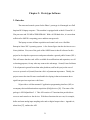
Chapter 1: Introduction
1.1 The SuPER Project
The Sustainable Power for Electrical Resources project was born in July of 2005
with Dr. James Harris’ white paper describing a durable, low-cost, family owned solar
power system [1]. It is intended as a self-contained and self-monitoring off-grid DC
system with energy storage capability that will service a wide variety of loads. It was
anticipated that development time of the system would be around five years, with the first
three years dedicated to research, design, and the building of a prototype system. A goal
of SuPER is to demonstrate that the system can extend component life, especially that of
the battery, and achieve very low failure rate. It is expected that SuPER will be used by
family units in low-income, high-insolation areas of the world.
1.2 Personal Involvement
I first learned about the SuPER project at a presentation made by Dr. James Harris
at one of the Friday afternoon sessions of the department’s weekly graduate student
seminars. Photovoltaic cells are a fascinating technology, and though I knew very little
about power generation and distribution it was clear that the call for a digital control
system could use some computer engineering expertise. I began meeting with the
development team in January 2006, which is about the time construction of the project
prototype began.
My contributions to the effort for the first six months of my association with the
project consisted largely of support for Eran Tal, working on his thesis [2]. Readers new
1
to SuPER ought to become familiar with Tal’s work, as he led the team in building the
first stage of the prototype and provided a foundation for all that has been accomplished
since. During this period, I provided some software expertise to the team in doing some
C and assembly language programming, as well as managing the Linux development
environment on the project computers.
Since Tal graduated in summer 2006 and I took over project leadership, SuPER
has been a whirlwind learning experience for me. My educational and professional
engineering experiences have largely fallen under the programmable logic, embedded
systems and signal processing disciplines. I have never been a power and control
systems engineer or a proficient analog circuit designer, yet while working on SuPER I
have found a need to be a little bit of each of these in order to reach both personal and
team objectives. That is perhaps the most rewarding part of the entire experience. The
knowledge gained working on this project has added significant breadth to my pool of
engineering resources and tools.
1.3 Solar Power Systems
In section 2.1 of Tal’s 2006 thesis paper [2], he convincingly outlines the case for
SuPER; only a summary of his arguments will be presented here. There are
multitudinous opinions on whether or not rising global temperatures are directly caused
by human activity; regardless of the cause, it is nevertheless a fact that atmospheric
carbon dioxide levels, and by extension, temperatures, have been sharply on the rise in
the last 25 years [3]. Such changes will have consequences for life on this planet as we
know it. SuPER harvests energy from a renewable source, and contributes no direct air
pollution to the environment. It is a device designed with the goal of sustainability in
2
mind. It is also intended to be a low-cost system (which will “pay for itself” within a
short time of activation [1]) in order to provide advantages to lower income families who
have not previously had access to a power generation system. There is no grid
infrastructure required as all issues associated with long distance power distribution are
removed as costs, obstacles, and energy sinks.
Solar cell technology is becoming increasingly important as an energy source for
reasons alluded to above. As a result, it is also becoming a more ubiquitous, better
researched, more efficient and more cost-effective technology [4]. The technology is
quickly developing into a preferable option among those in SuPER’s target market,
where cooking, heating and lighting energy needs are largely still provided by fossil-fuels
[5].
There are a few commercially-available solar power systems similar in scope to
SuPER, such as those manufactured by SunWize (www.sunwize.com). SuPER is an
attempt to develop one of these types of systems at much lower cost, and the team
anticipates future advancements in technology that will make this possible. This is
especially true of solar cell and battery technology. What is unique about SuPER is how
it is put together, and perhaps more importantly, why.
In [6] Sharaf and Ul Haque present a DC motor solar power system, along with
Simulink models, but there is no storage in the system. In [7] by Chiang, Chang, and
Yen a system very similar to SuPER is proposed and prototyped, although it is designed
to be a supplement to grid power rather than a replacement. This is the case with many
commercial systems. For related reasons the authors are unconcerned with managing
individual loads and optimizing battery life. There are countless additional published
3
papers that address a wide variety of other issues with the components that make up
SuPER, including, but not limited to, converter topologies, battery state of charge (SOC)
measurement, and maximum power point tracking (MPPT) techniques. Most
publications referenced by the SuPER team do not propose or demonstrate a system on
the scale of the SuPER project.
1.4 Thesis Objectives
The broader focus of the work carried out on this thesis project is the effort to
build a reliable, self-monitoring and adjusting 150W solar powered DC plant and
distribution system. In these early stages of development, the loads considered are a
small television, electric cooler, LEDs for lighting, laptop, and permanent magnet motor.
The first seven months of the SuPER team’s efforts resulted in a partially complete openloop system dubbed Phase 0. The white paper mentions the goal of achieving a complete
prototype system, Phase 1, within one year of commencement. A few months into
project work, the team felt confident in reaching and even exceeding that goal. However,
the development of the DC-DC converter, a crucial subsystem, hit a few road blocks.
Phase 1 was not achieved by the end of 2006 as expected, nor was it by March 2007
despite the fact that new converter teams came on board in October 2006 and February
2007.
As a result of these hardware setbacks, we were inclined to turn our attention
towards other efforts for the time being. The software for the status and control system,
written in C, was developed as necessary in preparation for the integration of the
converter. The SuPER team also recognized the knowledge that can be gained in
simulating such a complex system in computer software, and this thesis presents a
4
complete first generation system model. Such a simulation can reveal what types of load
scenarios a 150W panel can support, establish load time and power boundaries, and
provide information on how and when to best utilize battery energy storage while
maximizing the life of the battery. The simulation will also be critical for making plans
for scaling the system up in size (power). The goal of the thesis is to show that a virtual
mathematical model of the entire system compares favorably with a prototype system
constructed entirely by students (with faculty and staff guidance). Simulink, with its
SimPowerSystems model package, is used regularly in industry as a power and control
system simulation tool and has been chosen for the SuPER simulation.
Achieving this goal will require characterization of the DC loads and careful
study of prototype performance so as to allow proper modeling in Simulink As such, the
majority of the work done by the author during fall 2006 and winter 2007 quarters has
been in these areas:
1) constructing the Simulink model and simulating the system
2) developing the framework for the prototype status and control system software
3) testing the system operationally under a variety of load conditions
4) characterizing the loads
5) solving both hardware and software bugs that have periodically arisen
6) coordinating and supporting the undergraduate students working on senior
projects associated with SuPER
1.5 Document Overview
Chapter two introduces the SuPER system prototype as it existed in the fall of
2006; included is information about the loads which SuPER will power and specifics
5
about the team’s approach to battery management, which becomes a very sensitive issue.
Some of the requirements for the next generation of the system are presented, which will
provide an understanding of what the SuPER team hoped to accomplish by the end of
March 2007.
Chapter three provides the details for the software of the prototype’s status and
control system, the real brains of SuPER. The system consists of a series of sensors
which feed data into a laptop computer for computations and convey corresponding
output signals to control various components.
Chapter four represents the bulk of the work done by the author, which was the
creation of a MATLAB Simulink model of the entire SuPER system. Each part of the
model is presented, and design decisions defended.
Chapter five describes through examples how the simulation is used to estimate
the optimal control strategies to be put into use with the prototype’s control system. A
comparison of measurements of the prototype in action and simulation results is made for
multiple load scenarios.
The final chapter gives closure to things learned and conclusions determined from
the experiences of this thesis work. Recommendations are made for the future as part of
a review on problems that have now been neatly defined thanks to the progress made on
SuPER in the last six months.
Appendices at the very end of the document are a repository for information
pertinent to the success of SuPER but supplementary in nature to this thesis.
6
Chapter 2: Background
2.1 Phase 0 Prototype
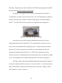
Tal spearheaded the effort throughout the first half of 2006 to assemble the first
SuPER system. The resulting system is a completely functional prototype, and the
current state of the system is known as the Phase 0 system (Figure 2.1).
Figure 2.1 - Photo of SuPER Cart, Associated Loads
SuPER consists of a PV array, DC-DC converter, storage battery, and DC loads.
Batteries are one of the most expensive components in the system as they cannot be
manufactured on campus. Two of the key loads in the system, a water pump and small
refrigerator, are intended to be run primarily during hours of peak insolation, but the
SuPER team also considers evening lighting to be an essential load. The improvement in
7
safety and reliability of electrical lighting over fossil-fuel consuming sources is worth the
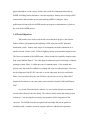
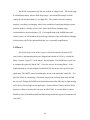
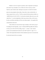
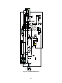
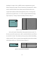
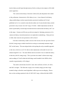
additional cost and complexity of including battery storage. Figure 2.2 is the Phase 0
block diagram.
VL
IL
Loads
MAX622 High
Side Driver w\
MM74C903 Hex
Buffer
PVI1090
High Side
Driver
V2
I2
V3
I3
T2
T1
T3
Outback MX-60
PV Panel 150W
V1
Battery 12V
I1
PWM Signal
(Open Loop Response)
PV Out
USB Interface
USB 6009
DC-DC Out
PC
Switch
Toggle and
Sensor CCode
Loads
T1
MPPT charge
control
algorithm Ccode
PIC Microcontroller
T2
T3
V1
This block diagram varies
from the Phase 1 block
diagram in only two places:
1) Outback MX-60 instead of
DC-DC converter.
2) Open loop PWM signal,
since there is no DC-DC
converter to interface it with.
V2
I1
V3
I2
PWM duty
cycle and serial
communication
C-Code
VL
I3
IL
Serial
Interface
TTL-toSerial
Converter
Stage: Integrate all
individual system
components to one unit on
the cart
Figure 2.2 - Phase 0 Block Diagram [2]
The Phase 0 system uses the MX60, a high-capacity DC-DC converter
manufactured by Outback Power Systems, to buck the voltage level from the PV array to
the desired 12V level on the load and battery bus. The MX60 is not simply a converter,
but also an MPPT charge controller. This feature has been critical for this early period of
prototype development.
8
2.1.1 Power and Distribution
It was hoped that the Phase 0 system would provide about 400Wh of energy per
day. About half of that was earmarked for the 187W DC motor, while the remainder
would service the battery and all other loads. However, the motor’s output rating is
187W. The permanent magnet motor is not 100% efficient, and to produce 187W of
power the motor requires more than 240W of input power. In addition, the laptop needs
to be running at all times throughout the day and requires at least 240Wh for an eight
hour run. As such, the priorities of the Phase 1 control system needed to be reconsidered,
and this will be discussed in later chapters.
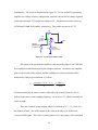
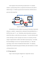
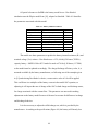
See Figure 2.3 for the Phase 0/1 power flow diagram. Power consumed by sensor
and switch boards, lost in cable and switch resistances, or otherwise unaccounted for and
attributed to system losses, is significant and preliminary loss investigations will be
presented in chapter five.
Figure 2.3 – SuPER Power Flow Diagram
9
During previous work on SuPER, the team had somehow overlooked the
problematic issue of high current (which we will call current above five amps) traversing
the copper traces on the switch board PCB. This was not realized until motor testing one
afternoon. The load torque was increased to about 4 lb·in, which was higher than
previously tested values. At this level the motor seeks to draw upwards of seven amps,
perhaps eight or nine, depending on the load bus voltage. It turns out that the PCB traces
were thick enough only for about five amps, and the increased current caused the traces
to heat up and melt the solder joints at the MOSFET. This in turn created a short at the
MOSFET terminals. The problem was first noticed when the status system reported a
draw of 39A from the battery (due to the newly created short), which would be possible
in a scenario with many running loads, but highly abnormal and great cause for alarm in
this particular case. In addition, it was unexpected to see such a draw because some
measure of protection had been expected from the circuit breakers in the breaker box.
However, the team failed to account for the slow response of breakers to negotiating
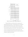
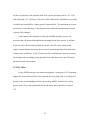
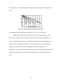
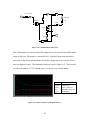
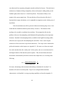
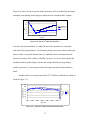
currents above breaker ratings. Breakers do not, in fact, mimic fuses in functionality.
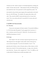
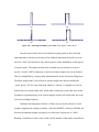
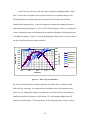
Their response instead obeys the tripping time curve seen in Figure 2.4. Thus, for the
30A breaker in use on the hot battery line, a 39A draw is just under 130% of rated
current. At that level, it would have taken one minute for the breaker to trip. It was
never given a chance as the problem was discovered and the system shut down manually
in a matter of a few seconds.
10
Figure 2.4 - Circuit Breaker Industries (CBI) Breaker Response Curve
One particular breaker, on the DC motor load line, was replaced by a fuse.
Largely motivated by this experience, it was determined that as soon as reasonable, the
original switchboard should be replaced by smaller, modular boards each crafted to
handle certain amounts of current. Such modularity would have the added benefit of
improving troubleshooting and repair turn-around time. As part of this process, it will be
necessary to learn about the design and manufacture of high current PCBs. Kaha
Sariashvili joined SuPER in January 2007 to design and test a board for the motor load,
and suggest new designs for the switch board.
11
2.1.2 Status and Control Hardware
A/D conversion for data acquisition is accomplished by use of multiple National
Instruments’ (NI) USB-6009 Multifunction Data Acquisition (DAQ) devices. As
indicated, they interface to a PC host via USB. All data that provides system status
information to the PC for control comes in through these devices. The network of
sensors, data acquisition devices, and PC software that manages the devices and data is
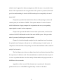
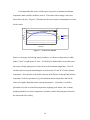
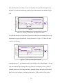
collectively known as the SuPER status system. Figure 2.5 shows a simple block
diagram of this system. The hardware of this system in its current state is partly the work
of Gustavo Vasquez, as documented in his Spring 2006 senior project paper [8].
Figure 2.5 – Status System Interface Block Diagram [8]
There is a triple of key sensors (voltage, current, and temperature) at each of three
essential locations in the system: the PV array, the DC-DC converter output, and the
battery. In addition, the voltage and current are monitored at each load. Newly added in
recent months is a pyranometer which outputs a voltage level corresponding to the level
of insolation. Therefore the total number of status system inputs, M, is defined as: M =
10 + 2·L where L is the number of loads.
The current sensors used are the ZAP25 and AMP50 models manufactured by
Amploc. Temperature data is provided by National Semiconductor’s LM50 sensor.
12
Vasquez’s efforts included sensor characterization and calibration, the construction of
sensor circuit boards, and work on the status system data reading code. The sensor
circuit boards are for converting the current and temperature sensor output voltages to
proper levels for the A/D inputs. Also, the subsystem voltage levels are stepped down to
required levels for the USB-6009 devices.
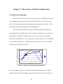
The pyranometer is manufactured by Apogee Instruments, Inc. and measures the
insolation, which is the radiation between wavelengths of 300 and 1100nm incident to the
Earth’s surface [9]. The level of insolation outside the earth’s atmosphere has been
measured at 1370 watts per square meter (Wm-2) [10]. The level incident to the earth’s
surface is less due to atmospheric attenuation and other factors, and the maximum
terrestrial insolation observed by SuPER team members is just under 1100Wm-2. There
is a reduction in incident insolation as the angle between the normal to the sun’s rays and
the line of propagation of rays to the point of measurement increases. Thus, equatorial
regions receive greater insolation than other regions of the planet in general. The amount
of reduction corresponds directly to the angle and this effect is expressed mathematically
as Lambert’s cosine law [9]; for this reason Apogee instructs that the pyranometer must
be mounted parallel to the ground. The pyranometer is calibrated to output 1mV per
5Wm-2, or a maximum of 220mV at the full insolation level of 1100Wm-2. The value of
5Wm-2 in this ratio is determined by fabrication methods and materials, and is inscribed
upon the device by the manufacturer. The manufacturer reports a temperature sensitivity
of about .1% per degree C, for which we do not compensate at this time.
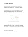
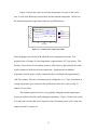
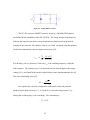
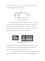
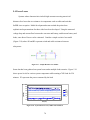
A circuit for amplifying the pyranometer output was constructed on a breadboard
attached to the inner wall of the switch box, an effort supported by senior Slavic
13
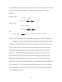
Orzhakovsky. The circuit is diagrammed in Figure 2.6. We use an LM324 operational
amplifier in a voltage reference configuration, powered with an LM340 voltage regulator
which steps down the 12V system bus voltage to 5V. The measured resistor values are
9.87kΩ and 2.18kΩ for R1 and R2, respectively. This results in a gain A of 5.52.
10k
R1
2.2k
R2
Vout
LM324
Apogee
pyranometer
0 - 220 mV
5V
LM340
Regulator
(from 12V bus)
Figure 2.6 – Pyranometer Data Circuit
The output of the pyranometer amplifier is fed into analog input #7 on USB-6009
Dev1 and data recorded and stored by the computer software. In software, the amplifier
gain A will be removed by division, and the resulting raw value in millivolts will be
multiplied by 5000 to give insolation, G, in Wm-2.
G =
multiplier ⋅ W / m 2 / V ⋅ V in
A
=
5 ⋅ 1000 ⋅ V in
5.52
All data produced by the status system is collected by the control system at a rate fss,
defined as the status system sampling frequency. Its inverse is Tss, which is currently set
at two seconds.
There are N control system outputs where N is defined as N = 3 + L, where L is
the number of loads. One of the outputs is the value of the duty cycle for the buck
converter PWM signal. This value is usually spoken of as a percentage, with a minimum
14
of 0 and a max of 100. In the PC software it is stored and manipulated as a floating point
number, with values between 0 and 1. When transmitted serially to the PWM-producing
microcontroller the value is first represented as an 8-bit unsigned binary number. The
microcontroller code provides the proper mapping of the unsigned number to the desired
duty cycle of the PWM output. The remainder of the outputs produce binary on/off
values. These control the MOSFET switches that dictate the flow of current in the
system. There is one switch each for the PV array and DC-DC converter, and one for
each load circuit.
2.2 SuPER Load Characterization
2.2.1 Television
The television is the simplest of all loads considered. The unit which SuPER uses
is a 12V DC black/white GPX portable TV/radio, equipped with a 5-inch screen. It
draws a continuous current of between 600 - 700mA (8W). The television circuit is
identified on the prototype as circuit #2.
2.2.2 Cooler
The Coleman 12V DC cooler was chosen to represent a typical low-power (6070W) refrigeration device that might be used by families who have had no previous
access to in-home refrigeration. The cooler load is identified as circuit #3. This
particular model (5644) has a volume of 40 quarts, and uses a Peltier element to cool the
interior down to about 40° F below ambient temperature. An empty cooler reaches this
state in three hours. The power cable is equipped with a 7.5A fuse. For SuPER we wish
to study methods of limiting the power needed in operating the cooler.
15
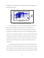
It was hoped that the cooler would require less power to maintain a minimum
temperature than would be needed to reach it. Tests done with an empty cooler have
shown this to be true. Figure 2.7 illustrates the decrease in power consumption over time
50
45
40
35
30
25
20
15
10
5
0
.
70
60
power (W)
50
40
30
20
10
0
10
60
110
temp (F)
80
.
for the cooler.
Power
deltaT [F]
160
time (min)
Figure 2.7 – Cooler Power Demand
However, an empty cooler being largely worthless, we choose to characterize it while
under a “load” of eight quarts of water. It will likely be undesirable to invest the power
necessary to bring eight quarts of water down to the minimum temperature. We will
simulate and test towards maintaining the water between 20° and 30° F below ambient
temperature. Note that due to the Peltier element, the difference in internal and ambient
temperature is the key parameter [11]; the minimum interior temperature that can be
achieved is highly dependent on the external temperature. If possible, it would be
preferable to be able to control the temperature assigning some initial value, without
sampling internal air or water temperature, and make control decisions purely based on
the time needed for cooling.
16
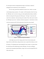
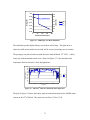
Figure 2.8 shows the cooler air and water temperature over time as the cooler
runs, as well as the difference between those and the ambient temperature. In this case,
the ambient temperature experiences relatively small fluctuations.
temp (F)
.
70
60
50
water
40
cooler air
30
diff(ambient,int air)
20
diff(ambient,water)
10
0
0
50
100
150
200
time (min)
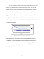
Figure 2.8 – Loaded Cooler Temperature Study
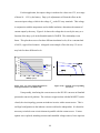
Most intriguing is the linearity with which the water temperature decreases. The
downward rate of change of water temperature is approximately .05°F per minute. This
linearity is also observed in a warming scenario; chilled water is placed inside the cooler,
which contains air chilled to the same temperature. Equalization with ambient
temperature (which, again, is fairly constant) has been calculated to be approximately
.008°F per minute. The ratio of warming rate to cooling rate is .16. Thus, to maintain an
average temperature, power theoretically need be delivered to the cooler for only 8.3
minutes of every hour.
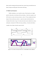
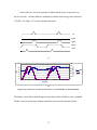
This characterization is fine for very gradually changing external temperatures,
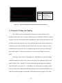
but proves all but useless for rapidly changing temperatures. Figure 2.9 shows the results
of a study done in which the cooler experiences three 60-minute power cycles, each nine
minutes on and 51 minutes off.
17
100
90
80
70
diff(ambient,water)
temp (F)
60
ambient
cooler air
50
40
cooler water
30
20
10
0
0
50
100
150
200
time (min)
Figure 2.9 – Cooler 60-minute Cycle Temperature Study
The cooler on times can be identified by the corresponding drops in interior air
temperature. One problem with this cycle period is the time taken for the interior air
temperature to drop low enough to begin to cool the water, a sort of “setup time”. It is
likely more efficient to increase the cycle period so that setup times are a smaller ratio to
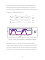
total cooling time. A second study, with measurements plotted in Figure 2.10, extends
the cycle period to 725 minutes. The cooling period occurs in the first 100 minutes.
80
70
60
temp (F)
50
diff(ambient,water)
ambient
40
cooler air
cooler water
30
20
10
0
0
100
200
300
400
500
600
700
time (min)
Figure 2.10 – Cooler 725-minute Cycle Temperature Study
At time 538 minutes, the cooler was brought indoors to provide a more constant external
temperature, for reference and comparison purposes. The much more steady temperature
difference rate of decline from that point onwards is clear. It can also be observed that
18
the quickly increasing external temperature has a high impact on the rate of change of
internal cooler air temperature when the cooler is unpowered. Maintaining some average
difference between ambient and water temperature is difficult under variable conditions.
If the cooler is to be run out of doors, it may be necessary to power the cooler much more
often than desired. If that is accepted, perhaps some power savings can still be achieved
while measuring only the ambient temperature and compensating by adjusting run times.
2.2.3 LED Lights
One of the primary functions of SuPER will be to provide a few hours of nighttime lighting for the family home. The necessary energy will be drawn from the battery.
It is expected that the control system will ensure that the day ends with the battery in a
high SOC in anticipation of the energy requirements for lighting. It is essential however
to find a type of lighting that provides high output, usually measured in lumens, at
minimum energy use. To this end, SuPER will rely on the emerging LED lighting
industry. The LEDs available today use about 3W of power and generate around 100
lumens each [12]. Unfortunately, operating at this wattage is inefficient. The SuPER
prototype will instead operate the lights at a tad over 1W apiece. Four such LEDs will be
allocated for use for the immediate future, requiring approximately 4.5W of power. The
lights are designated as circuit #4.
2.2.4 Laptop
System status and control is run on a Dell Inspiron B120 laptop, chosen for its
low cost (under $500). Specifications for the device declare it to be a 60W max system,
drawing about 3A at about 20V. A converter is thus required for the 12V SuPER system
19
bus to which the laptop will connect. A Lind Electronics Model # DE2035-966 converter
was purchased from Dell; this converter will turn a 12-32V DC input into a 20V DC
output at a maximum of 3.5A. It is equipped with a 15A fuse. Figure 2.11 shows the
converter.
Figure 2.11 – Lind Electronics Model # DE2035-966 Converter
Information about the power and battery management system on Dell’s laptops is
proprietary, and therefore not available to the public. However, regular observation of
the system in operation reveals some useful trends. The approximate battery SOC while
charging from a wall outlet is recorded using the Windows XP battery meter, and
displayed against time in Figure 2.12.
100
SOC (%)
90
80
70
60
50
40
30
20
10
0
0
20
40
60
80
100
120
time (min)
Figure 2.12 – Laptop Battery SOC Under AC Power
When powered by the SuPER cart, without its internal battery, the laptop draws
approximately 2.5A (as considered from a system perspective and hence concomitant to a
potential of 12V). With the laptop battery inserted, the behavior seems to change relative
20
to the SOC of the battery. A depleted battery will perforce need to be charged, so the
laptop will draw enough current to run the device and charge the battery in tandem. The
laptop circuit will in this case draw two extra amps, for a total of 4 to 4.5A, which is
closer to the specified maximum power requirement. With enough time passed to
anticipate a fully charged internal battery, it is observed that the laptop has again reverted
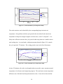
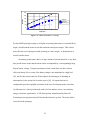
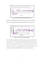
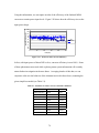
to a 2.5A current draw. Recorded data (see Figure 2.13) shows that there is a gradual
drop-off in the current drawn by the laptop. Using the data from Figure 2.12, we can
predict the time at which the battery reaches approximately 80% of charge capacity.
80% SOC
60
55
power (W)
50
45
40
35
30
25
20
0
50
time (min)
100
150
Figure 2.13 – Observed Laptop Power Needs Under Solar Power
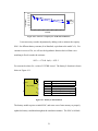
This is fairly consistent with the known charging current requirements for lithium-ion
batteries [13]. Lithium-ion batteries do not require a low-current trickle or float charge,
and in fact may be damaged by such. Thus, the charge cutoff current is to be 0A. Figure
charging current
2.14 gives the shape of the expected lithium-ion battery charge current over time.
time
Figure 2.14 – Lithium-ion Battery Charging Current as a Function of Time
21
For the vast majority of the operation time of the system, the laptop will be a 30 – 35W
load rather than a 54 – 60W load. This issue will be addressed in simulation by providing
a variable load controlled by a laptop-specific function block. The mechanism is present
for future use, but at this stage of development of the model the laptop battery is treated
as always fully charged.
As the laptop is the intelligence of the entire SuPER prototype system, it is
necessary that it be powered throughout the operating period of the system. It will thus
be the last load to be disconnected from the system. We will not be relying on the
laptop’s internal lithium-ion battery for any sort of sustained operation of the status and
control system at this time. It will of course provide a small amount of power-on current
for the laptop when initiating system operation from a shut down state, and will only be
depended upon for that purpose.
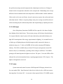
2.2.5 DC Motor
For the SuPER prototype, the team has equipped a ¼ horsepower, 12V permanent
magnet DC motor which will be used to represent the water pump load. It is anticipated
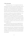
that this is the most demanding load to be powered by SuPER. Jennifer Cao’s senior
project report [14] records operational data for the motor, also echoed here in Figure
2.15.
22
250
200
power (W)
150
power in
power out
efficiency (%)
100
50
0
0
2
4
6
8
10
torque (lb*in)
Figure 2.15 – Motor Load Power vs. Torque
For the SuPER prototype testing we will plan on operating the motor at a constant 8lb·in
torque, which loads the motor to near the maximum rated power output. This is also a
more efficient use of input power than operating at a lower torque. A dynamometer is
used to load the motor.
On starting up the motor, there is a large amount of current drawn for a very short
time period known as the inrush current, and is accompanied by a correspondingly large
drop in battery voltage. Frequent repetitions of such current draw can have adverse
effects on battery life over time if the battery charge is not maintained at a high level
[15], and for this reason senior Joe Witts explores the advantages of including an
ultracapacitor in the system for his senior project [16]. He reports that such a
configuration provides negligible assistance in the case of infrequent motor activation.
Cycled motor use, with a period on the order of a few minutes or less, can cut battery
energy costs down significantly. A 58F ultracapacitor manufactured by Maxwell
Technologies was purchased and will be introduced into the system. The motor load is
circuit #6 on the prototype.
23
2.3 Battery Management
The SuPER prototype battery is a 12V valve-regulated lead-acid (VRLA) unit
manufactured by East Penn (or Deka), rated at 98Ah for 20 hour discharge. The SOC of
a lead-acid battery is a percentage representing the ratio of charge remaining to total
battery charge. Its inverse is the depth of discharge (DOD). Determining the SOC for
VRLA batteries while connected to a load has always been a difficult problem. The
simplest, most typical way to make this determination in practice is to measure the opencircuit voltage (Voc) of the battery, due to a nearly linear relationship between Voc and
SOC for lead-acid batteries [15]. This method provides a reasonably accurate
assessment, however, it is unrealistic for many systems because a true Voc can only be
attained after all current flow in and out of the battery has been suspended for 24 hours
[15]. This is not an option for the SuPER project. The general approach to this problem
is to use frequent measurement techniques to estimate the SOC in software. Methods to
this end are proposed by Vairamohan in [17], Duryea, Islam and Lawrence in [18], and
Castaner and Silvestre in [19].
The SuPER team has chosen to use the model in [19] designed for PSpice but
modified by team member Tyson Den Herder for Simulink as his senior project [20].
This model is divided into charge and discharge mode and provides a SOC estimation
using the battery energy balance equation. Upon integration of the student-designed DCDC converter, it is anticipated that this model will be ported to C code on the status and
control laptop. In [21] Fasih provides some vindication of the model and methodology.
Like SuPER, Fasih also made use of Hall effect current sensors and NI DAQ hardware
for his measurements.
24
One shortcoming of the model in [19] is that it disregards the non-trivial impact of
temperature on the battery state. Also, Castaner and Silvestre mention that the model
realistically should be restricted to use for a SOC within a range of 30-80% of capacity,
for which it will provide the best estimates. This provides a problem for SuPER, as we
desire to always maintain as high a SOC as possible. The approach taken to this matter is
detailed in chapter four.
Tal’s thesis [2] Appendix B discusses the way battery charging is handled by the
Outback MX60 converter. The device relies solely on PV and battery voltages for its
calculations, as we will do with the Phase 1 system. Our goal will be to mimic the
operation of the MX60 with our converter. The MX60 is a very expensive (and efficient)
piece of hardware that was designed to handle much larger amounts of power than that
associated with the SuPER prototype [22], [23]. It has three primary charge states: bulk,
absorb, and float. While in the absorb stage, the MX60 gradually reduces current over
time, and assuming plenty of available current will run approximately one hour. The
battery documentation prescribes charging voltage levels for bulk and float stages (Figure
2.16), but makes no mention of an absorb stage.
Table 2.1 – Deka Battery Charge Voltage Guide [15]
25
The MX60 is programmed by the user with these voltage levels. The absorb stage
is entered immediately after the bulk charge stage. Absorb and float stages are both
employed only when the battery is in a high SOC. The primary concern for battery
integrity is avoiding overcharging, which is the condition of supplying charging current
when the battery is already at 100% SOC; hence the different charging stages
recommended by the manufacturer [15]. For simplification of the SuPER status and
control system, we will abandon the absorb stage and utilize only bulk and float charging.
In discussions with Tal, he indicated that this was a reasonable simplification.
2.4 Phase 1
The closed-loop version of the system, in which all modules (besides the PV
array, battery, and laptop hardware) are designed and created at Cal Poly, is called the
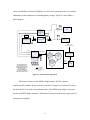
Phase 1 system. Figure 2.17 is the Phase 1 block diagram. The SuPER team’s goal was
to complete this phase by March 2007. Critical to success in reaching Phase 1 is the
implementation of a locally designed and built DC-DC buck converter specific to this
application. The MPPT control would then be moved to the status and control PC. Two
previous efforts at constructing a functional converter have already been made and did
not succeed. Perhaps the SuPER team had underestimated the difficulty in implementing
such a device for this high current application. Seniors Robert Casanova and Joe Shein
began new efforts to develop the converter in fall of 2006. A second effort by seniors
Thaddeus Guno, Koosh Shah and Kunal Shah using an alternate approach commenced in
early 2007.
26
VL
IL
Loads
MAX622 High
Side Driver w\
MM74C903 Hex
Buffer
PVI1090
High Side
Driver
V2
T1
T2
PV Panel 150W
DC-DC Converter
V1
I2
V3
I3
T3
Battery 12V
I1
PWM Signal
PV Out
PC
USB Interface
USB 6009
DC-DC Out
Switch
Toggle and
Sensor CCode
Loads
T1
T2
Full charge
control
algorithm Ccode (from
MATLAB)
PIC Microcontroller
T3
*Notes:
1) All loads and load probes
are represented as one in this
diagram.
2) All probes are connected
to the USB 6009 via an op
amp gain circuit, omitted
from this block diagram.
3) The combiner box, which
doesn’t appear in the block
diagram, junctions all the
power lines.
V1
V2
I1
V3
I2
PWM duty
cycle and serial
communication
C-Code
VL
I3
IL
Serial
Interface
TTL-toSerial
Converter
Stage: Integrate all
individual system
components to one unit on
the cart
Figure 2.16 – Phase 1 Block Diagram [2]
The specifications given for the converter, derived from PV array and battery
characteristics are:
Table 2.2 – DC-DC Converter Specifications [2]
Parameter
Input voltage
Input current
Max power
Output voltage
Output current
Switching frequency
Value
wide range, 0 to 40V
4.75A max
150W, 80% efficiency target
11.5 – 14V
13A max
500 kHz
27
See section 5.2.2 in [2] for more details on the specifications. Guno, Shah and
Shah are designing a converter from the ground up [24], and their efforts will include
layout of a high-current PCB. The 500 kHz PWM signal for this converter is sourced by
a microcontroller, and some of the difficulties with this approach involve proper marriage
of this signal to the MOSFET switch. Casanova and Shein are using an entirely different
method [25]. SuPER has been provided with dual 75W buck converters as a donation
from Linear Technology. These converters have a built-in PWM signal generation chip,
which uses a resistive feedback line to maintain a constant 12V output. Some
modifications were necessary to apply the device to SuPER, as the output cannot be
constant due to the battery and loads. It was theorized that using different values of
resistors on the feedback line would alter the response of the PWM generator chip and
could be used to adjust the output voltage of the converter. Casanova and Shein proved
this true, and a Maxim digital potentiometer (MAX5529) controlled by a two-wire serial
interface is used to provide the changing resistance. Its 64-tap configuration will allow a
1.56% duty cycle resolution. Control of the potentiometer will be via the digital output
ports on the USB-6009 device. Code written to communicate with the potentiometer
(potcomm.c) has been tested successfully.
Perhaps the most useful of the proposed power sinks for SuPER, the LED lighting
remained an untouched matter through the summer of 2006. LED lights are a continually
evolving (and also pricey) technology; nevertheless, the Phase 1 system provisions their
inclusion. The lights are the final of the five proposed loads the prototype will service in
these experimental stages, and senior Joey Zukowski was tasked with equipping the
devices for SuPER at highest energy efficiency.
28
An additional Phase 1 goal is the development of a user-independent control
system which derives maximum use of each load while optimizing the life of the battery
and preventing overcharging. Essential to the development of an optimal control system
is a thorough understanding of system behaviors under a variety of conditions. It is
therefore desirable to simulate the system and create a platform upon which control
schemes can be developed, assessed, and adjusted as necessary. This ambition became
increasingly important to the project as it became clear that the integration of the DC-DC
converter would not be reached on schedule.
As mentioned previously, there was a misstep in plans for handling the system’s
current requirements on the switch board in the Phase 0 system. For a completely
operational Phase 1 system, the issue must be solved. The team also determined to take
advantage of these efforts to simultaneously increase the modularity of the system
components; specifically, it would be valuable to physically separate PCBs of different
purposes and current levels.
As summarized in Table 2.3, besides the work on the ultracapacitor, seven
parallel efforts were made from October 2006 through March 2007 to reach the Phase 1
plateau. Some of the work by these Cal Poly seniors will require the inclusion of more
digital control system outputs in the near future. Zukowski will develop a DC-DC
converter to step down from the 12V bus voltage and deliver about 4.5W to four LEDs.
The PWM will also be transmitted by the PC through the PIC and managed by voltage
and current monitoring code, in order to achieve maximum efficiency with the LEDs.
The PIC can provide two PWM outputs if need be. For immediate integration and
testing, a purchased static-output buck converter will provide satisfactory output.
29
Table 2.3 – 2006-2007 SuPER Project Student Contributions
Project
DC-DC converter development
(device modification)
DC-DC converter development
(computer-controlled)
High current PCB development,
thermocouples
Pyranometer integration
High current PCB development
Simulation and software control
LED lights subsystem integration
Ultracapacitor integration
Student Contributors
Robert Casanova
Joe Shein
Thaddeus Guno
Koosh Shah
Kunal Shah
Shane Murphy*
Juan Uribe*
Slavic Orzhakovsky*
Kaha Sariashvili
Tyler Sheffield
Joey Zukowski
Joseph Witts
* denotes independent study, as opposed to senior project contributors
Though his efforts are not associated with the Phase 1 objectives, Joe Witts will add an
ultracapacitor between the battery and the loads and will need control signals for three
switches to manage the charging and discharging of the capacitor. The main converter
built by Casanova and Shein will require two digital outputs for a serial interface to a
digital potentiometer.
30
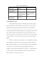
Chapter 3: Prototype Software
3.1 Interface
The status and control system for the Phase 1 prototype is all managed on a Dell
Inspiron B120 laptop computer. This machine is equipped with an Intel Celeron M 1.4
Ghz processor and 256 MB of DDR SDRAM. With a 40 GB hard drive, it is more than
sufficient for SuPER’s computing power and data storage needs.
The laptop executes all data acquisition and control code over a Red Hat
Enterprise Linux WS 3 operating system. A few factors figure into the decision to use a
Linux platform. First, one of the goals of the SuPER team is that all software for this
project be developed as open-source and protected under a general public license (GPL).
This will ensure that the work will be available for modifications and expansion, as well
as learning purposes, for any who may want to take advantage. Second, Linux facilitates
C development in general better than other platforms, and for this project the ease of
access to system-level (kernel) function calls is of paramount importance. Thirdly, the
project team at the time felt most comfortable developing in that environment due to
significant previous experience with Linux.
NI provides a well-documented C application programming interface (API) to
accompany their multifunction data acquisition (DAQ) devices [26]. The name of the
package is NI-DAQmxBase 2.1. This API consists of C functions that provide direct
access to and control over the devices. With these functions the user can, for example,
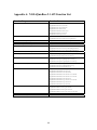
define and start analog input sampling tasks and set digital output values. Appendix A,
taken from [27], outlines the API.
31
The team encountered some trouble with Linux in regards to the integration and
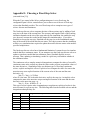
interface for the USB-6009 devices, and the lessons learned are mentioned in passing
here.
The Targus 4-port hub uses USB 2.0 drivers, so it is essential that the latest
version of the Linux kernel be installed on the host machine. Version 2.4.21-37 is not
equipped with the proper drivers and therefore version 2.4.21-47 must be installed.
Before halting execution of the interface software process, all tasks assigned to the
devices must be stopped and cleared. Bypassing this step causes a glitch that will result
in Linux losing the device identifiers; restoring functionality requires a device hard reset
(disconnecting the devices from their USB power source/host). Unfortunately, the
example code that NI ships with the devices, and upon which the SuPER code was built,
seems to disregard this peculiarity. As the NI code is executed, the user receives
instructions indicating that the process may be terminated by using the ‘ctrl-c’ command.
This is the universal Unix process halt command. This command does not allow the
process to exit gracefully, but ends its life by kernel override. As a result, the kernel
somehow loses communication with the DAQ devices. The problem was remedied by
adding code to alter the execution shell to return characters byte-by-byte from stdin with
each key press. When a ‘q’ is pressed, the loop catches it and is able to stop and clear all
active tasks before halting the process. See Table 3.1 for details on the USB-6009 device
errors encountered by the SuPER team.
32
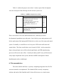
Table 3.1 – Known USB-6009 Errors
Error
Shell message: Device
identifier invalid
Shell message: Physical
channel specified does not
exist on this device
Shell message: Onboard
device memory overflow
Sensor readings are bogus,
such as large negative
temperature values
Implication
Linux has lost track of the
DAQ devices
No known cause
Action Required
Hard reset of DAQ devices
Host processes have taken
away system resources from
the USB-to-PC data transfer
(or less likely, the sample
rate is too high)
The device identifiers have
been mixed up
Close all other executables,
and do not run anything
besides status and control
program
Hard reset of DAQ devices
Hard reset of DAQ devices
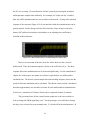
3.2 Functional Overview
All initialization and parameterization of NI-DAQ tasks is handled in function
main of the SuPER code, which is found in contAcquireNChan.c. The code enters an
unterminated while loop that repeatedly reads the values out of the storage buffers
recorded by the USB-6009, and displays them onscreen. Thousands of values are loaded
by the USB-6009 into the buffers, and the NUM_TO_OUTPUT definition fixes the
number of samples that are extracted (NUM_TO_OUTPUT must be less than or equal to
the integer bufferSize). The extracted values are all averaged to formulate the display
quantity.
The loop is executed at the system sample rate fss. At the beginning of each loop
cycle, the buffers are checked to see if the write time has been reached (as defined by
TIME_FACTOR, in minutes). The values must be periodically written to the hard drive
so as not to be lost. The written values consist of all samples extracted prior to
averaging. Thus, the written files contain NUM_TO_OUTPUT / Tss samples per sensor
for each second of run time and the total number of samples per sensor in the file is
TIME_FACTOR * 60 * NUM_TO_OUTPUT / Tss.
33
Hard drive accesses are expensive operations, and it is important not to delay the
time-sensitive loop commands so as to avoid the risk of device memory overflow.
Therefore, main is forked so that a child process may take care of the file I/O and the
parent can return promptly to data reading. Sensor data is written to the hard drive in
comma separated value (.csv) files. The files are named with date and time included, e.g.
“SuPER Wed Jan 10 10:44:30 2007.csv” and stored in a brother folder to the source code
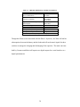
entitled data. To ease the manipulation of these large amounts of data, an Excel macro
has been created that consolidates the file into one minute samples. See Appendix B for
an introduction to this macro.
After each data set is observed and averages calculated a call is made to pnopal.c
for running the control algorithm. pnopal.c contains the MPPT algorithm and sends the
new duty cycle value to the PIC by calling commpic.c. commpic.c is the code that
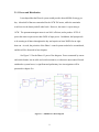
provides serial communication from the PC to the UART on the PIC. Figure 3.1 is a
software flow diagram that summarizes all the simultaneous processes in execution when
the status and control software are running.
34
USB-6009 RTOS
Register tasks
main
pnopal.c
forked main
commpic.c
Define,
create, and
start sampling
and digital
output tasks
write time
reached?
no
Microchip PIC
Power on
pwm
initialization,
set switching
frequency
yes
Dump all
accumulated
data to hard
drive
Send task
read
commands
Kill child
process
Sample inputs
and store data
Extract data
from storage
array
Display data
averages
Send task
write
command
Write
assigned
value to digital
output port
Pass saved
values to P&O
function
Execute P&O
MPPT
algorithm
Pass new
duty cycle
value to
comm code
Initialize
modem
connection
Convert duty
cycle value for
transmission
Transmit
value serially
to PIC
return
Figure 3.1 – SuPER Software Flow Diagram
35
return
UART
command
rxed?
Apply new
duty cycle to
PWM signal
yes
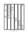
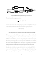
3.3 Control
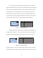
The diagram of Figure 3.2 details the locations of all Phase 0/1 control inputs and
outputs.
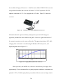
Figure 3.2 - SuPER Status and Control Interface Diagram
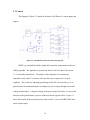
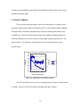
MPPT is accomplished with the simple and commonly-used perturb and observe
(P&O) algorithm. The algorithm is presented in detail in Aki Oi’s thesis [28] section
3.5.1, but briefly outlined here. The purpose of the algorithm is to maintain an
impedance seen by the PV array that will cause the array to output power at peak
capability. This is done by adjusting (perturbing) the DC-DC converter duty cycle at
periodic intervals and monitoring the resulting array power output, through current and
voltage measurements. A negative change in the power output will cause a reverse in the
direction of the perturbations; a positive difference has the opposite effect. Figure 3.3
shows the location of the maximum power point on the I,V curve of the BP150SX solar
panel at peak output.
36
Figure 3.3 – BP150SX I,V and Power Curves [28]
The status system sample period Tss (currently set at two seconds) puts a
maximum rate on the control algorithm execution. Note that this is entirely different
from the NI DAQ device A/D sample rate, which is much higher. Observation of the
performance of the MX60 converter shows rapid response times under quickly changing
conditions. The SuPER team attempts to mimic this capability, and will also run the
control algorithm at the maximum rate. It is anticipated that the host machine will have
adequate time to run the few necessary floating point multiplications and divisions
between samples and that computational time overruns will not be an issue. The DC-DC
converter transient response, discussed in more detail presently, will not be an issue at
this rate.
The prototype currently makes use of a PIC 18F4320 microcontroller which can
provide a 500 kHz PWM output. This is an upgrade from the 50 kHz signal provided by
the original Phase 0 hardware, a PIC 16F877A. The PIC code is written in assembly
language and compiled with the MPLAB development kit provided free of charge by
37
Microchip. Programming is achieved with the K128 USB 40-pin programmer from DIY
Electronic Kits (http://www.kitsrus.com/pic.html).
The laptop is not equipped with a serial port, so the connection to the PIC is
accomplished via a USB to serial conversion cable. The cable manufacturer is unknown,
but the conversion chip is a product of Prolific Technology Inc; the model number is
PL2303. Use of this cable in Linux requires driver installation and configuration.
Figure 3.4 - USB-Serial Cable with PL2303 Chip
It was necessary to develop a simple communication protocol for all serial
transmissions between the PC and the PIC. The communication is largely one way, as
the PC issues all commands and accompanying values. The microcontroller sends no
data to the PC, but does respond to successfully received commands and values by
returning an exclamation point character (!). UART serial communication is byteoriented, and for ease of implementation all commands and values are eight bits in length
or less. An explanation of the communication protocol can be found in Appendix C.
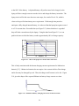
The battery model code from the Simulink model has been ported to the laptop, in
the form of a function called batt_voltage in contAcquireNChan.c. It currently monitors
battery current flow to estimate the actual battery SOC in real-time. Output is written
with frequency fss to Super_Output.csv.
38
The prototype control software is largely incomplete as some of the hardware
goals for the end of March 2007 were not attained. The only form of control currently
implemented in the prototype software is the MPPT algorithm; even so the generated
output is actually of no practical use without a DC-DC converter. The prime resource for
developing and testing control algorithms, then, is currently the Simulink simulation.
39
Chapter 4: MATLAB Simulink Model
4.1 Model Overview
The new Simulink system model builds upon the foundation established by Tyson
Den Herder in his senior project [20], but attempts to reach far beyond its limits and uses
a different development approach. The primary difference between Den Herder’s efforts
and what is to be accomplished in this thesis is a matter of construction, detail, and scale.
In the conclusion of his report, Den Herder makes some observations and
recommendations on improving the model, all of which are addressed in the model
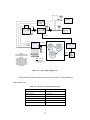
presented here. Figure 4.1 is a view of the entire SuPER Simulink Model.
40
Figure 4.1 – SuPER Simulink Model
Day Insolation/
Temp
Data Tables
TaC
G1
TaC
G1
Night Insolation/
Temp
Data Tables1
temp
ins
DCprev
Constant5
0
-
s
+
C
10 uF
cm
Paout
powergui
Discrete,
Ts = 5e-008 s.
charge_mode
count
Vb
arge_mode_out
control_plus
Vpv
Ppv
_c
Ipv
Controlled Current Source
G
TaC
PV_cIpv
Ipv
Vpv
1/z
Paout
.325
In1
pwm
d
g
Mosfet
s
m
Diode
dc_dc converter_ver2
Vpv
+
v
-
out1
PWM Gen SubsystemConstant4
cm
DC
+
-
C
3 uF
resistive loads
VC
v
.93 uH
Ic
+
i
-
set calculation rate
by changing block
sample time
SOC2
SOC
SOC1
Vbat
batt_voltage_c
V1
I1
R1
SOC
VS
IC
Vbat
IC3
set initial battery
Voc here
[12.844]
Vb
[.99]
assign initial battery
SOC here
cable
resistance
.02 ohms
Control Scope
V2
Ib
vbat
+
DC
+
i
s
DCout
3
Ic
Mean Scope1eT
u*9/5+32
eT
C->F
set to same as
LUTs
scenario
swcontrol_c switches
stime
cable
resistance
.02 ohms1
V_C
Load Scenario
Selector
Mean Scope2
Controlled
Voltage Source
Vb
+
v
-
12:34
Digital Clock
set to same as
LUTs
TV
8W
18 ohms
I_TV
T C Li La M
iT
LEDs
4.5 W
32 ohms
set initial
internal temp
diff (F)
Tdiff1 Tdiff2
diff
cooler_load_c
state
iTemp
eTemp
diff
1/z
Cooler
65 W
2.22 ohms
I_Cooler
[22.5]
i
-
DC
I_Laptop
g
1
m
2
i
-
laptop
30 W
4.8 ohms
[0]
how often to reset
running means,
(shortest sample
time)
Pulse
Generator
Rs
Up
tC
Cnt
set initial
LSOC here
[1]
1/z
swH
t
swL
aptop_load_
LSOC
LSOCout
sample times should
equal inso/temp
sample time (one-min)
Vb
Counter
IC4
[0]
IC2
== 0
laptop
Compare
55 W
To Zero
2.62 ohms
DC Motor
Steady State
237 W
.6061 ohms
IC6
[12]
g
1
m
2
set rate of change
of duty cycle by
setting block
sample time (doubleclick)
g
1
m
2
+
g
1
m
2
+
g
1
m
2
+
g
1
m
2
i
-
g
1
m
2
41
-
In
Rst
Ib
Mean5
In
Rst
Vb
Mean2
Ipv
In
Rst
Ipv
Mean3
In
Rst
Mean4
In
Rst
In
Rst
Mean
Ib
Vb
Ic
Vpv
Ipv
Mean Scope
Each component of the model will be presented in detail. For orientation
assistance, a generalized map of the key components and connections in the model is
offered in Figure 4.2. Red lines represent electrical connections, while blue lines are
purely inter-block signal lines.
Figure 4.2 - Simulink Model Map
In Simulink there are three methods of expressing the functionality of operational
subsystems, or modules: component blocks, mathematical function building blocks, or
MATLAB code (also C/C++,etc). Den Herder used the function block construction
method for the battery, control and converter subsystems. To assist the Simulink model
in better reflecting its real-life counterpart, the converter was recreated by Dr. Harris
using the component blocks available in the SimPowerSystems package. In a nutshell,
this means building the converter out of capacitors and inductors, etc., rather than
representing it with a collection of mathematical function blocks. For modularity,
reproducibility, and optimization purposes the battery and control modules were remade
as S-function blocks of code.
4.1.1 Design Approach
Figure 4.3 shows the typical configuration of a simple buck converter.
42
Figure 4.3 - Simple Buck Converter
The DC-DC converter MOSFET switch is driven by a 500 kHz PWM signal, a
rate defined by the capabilities of the PIC 18F4320. The energy storage components (an
inductor and capacitor) are the key converter parameters chosen based on the desired
response of the converter. The inductor value (L) is .93mH, calculated using the equation
for the desired maximum converter output current, from [29]:
⎡1
(1 − D ) ⎤
I max = V0 ⎢ +
⎥
⎣ R 2 ⋅ L ⋅ f sw ⎦
D is the duty cycle as a fraction of value one, fsw is the switching frequency, and R the
load resistance. The capacitor size (C) is determined by the desired ripple on the output
voltage (ΔVo), and found for this model with the help of some experimentation to be 3μF.
This is the relationship, from [29]:
ΔVo =
D ⋅ Vo
R ⋅ C ⋅ f sw
In a typical buck converter configuration with resistive loads, the potential
produced by the front-end source, Vs, is “bucked” to a desired average output Vo by
altering the switching duty cycle accordingly. The relationship is
___
VO = DVS
43
For this application, the output voltage is anchored to values near 12V, on a range
of about 10 – 14V, by the battery. Duty cycle adjustments will instead reflect on the
converter input voltage, which is the voltage Vpv at the PV array terminals. This voltage,
in conjunction with the temperature and available insolation, determines the amount of
current output by the array. Figure 4.4a shows the voltage that is seen by the array as a
function of the duty cycle in the Simulink model of SuPER. The relationship is not
linear. This plot shows curves for three different insolation levels, all at a constant load
of 68 W, a typical load scenario. Alongside is an example of how the array I,V curves
may look for these different levels.
50
Voc
45
35
high
30
moderate
25
low
Y-Axis
PV Array Voltage (V)
40
20
15
Vbatt
10
0
20
40
60
80
100
PWMDuty Cycle (%)
Figure 4.4 a) – PV Array Voltage Response for
Varying Insolation Levels (68W Load)
Figure 4.4 b) – Example of Corresponding
I,V Curves
Unexpectedly, interfacing the current source to the DC-DC converter in Simulink
presented a non-trivial problem. The software recognizes that with the MOSFET switch
closed, the circuit topology presents an inductor in series with a current source. This is
an illegal configuration as the inductor current would not be independent. It is therefore
necessary to include some circuit element in parallel with the current source. Various
options were explored, including resistors and controlled voltage sources, but a capacitor
44
actually provides the optimum system behavior. This is because the capacitor offers
stability in maintaining the converter input voltage, which is used to calculate the PV
array current. If the capacitor is too large, the response time will be too slow and the
voltage level will never rise; if too small, it does not provide the needed impact and the
voltage will fluctuate far too much. A good value for the capacitor was found by
experimentation to be on the order of microfarads, in this case 10μF. Thus, the Simulink
model includes an extra 10μF capacitor on the converter input due to the manner in which
the PV array is modeled for simulation purposes.
Voltages and currents plotted with Simulink scopes oscillate at the switching
frequency. The output voltage ripple is intended to be minimized by careful attention to
the capacitor chosen for the converter; to smooth the output to a greater extent and allow
the developer to see some semblance of average DC values, Simulink offers two options,
neither of which are ideal for this use. One option is the weighted moving average block.
Weights need to be assigned to each sample, and the number of weights determines the
“window” size. This makes it impractical for windows of thousands of samples, and has
proven difficult to use in practice. The chosen method is a reset enabled running mean
block, whose reset period is a confirmed hazard in simulation. The optimal period seems
to be twice the fastest S-function block sample period. The running mean blocks must be
reset on the falling edge of the reset signal, so that any downsampling does not catch the
block output early in the new mean processing, as the oscillations will result in unsettled
sampled values.
45
4.1.2 Function Blocks
Desiring a modular simulation model, we made prolific use of MATLAB’s Sfunctions. These are created as blocks in the Simulink model editor, but completely
defined by MATLAB code in associated m-files. There are a variety of S-function types,
but the original system design was done with these particular blocks; they are known as
Level II M-file S-functions. The function that is to be implemented can be written in
MATLAB language just as would be done for execution or function call from the
MATLAB command line. However, creating an S-function requires wrapper code
around that function code. Ports must be enumerated and identified for each input and
output of the block. The function code is placed in a separate section for determination
of the outputs. One drawback of these S-functions is their lack of internal memory. In
other words, the function is executed top-to-bottom continually with no memory of
previous states.
Efforts to speed up the simulation process led to a new approach to the Sfunctions. The software is greatly hampered by the need to call the M interpreter each
time M-file S-functions are invoked. By writing the code in C instead, and pre-compiling
it before runtime, the simulation time can be greatly reduced. This variety of function
block is known as a C-MEX S-function. Running one simulation on a 1.4 GHz machine
for the M code blocks required 22 hours. The same simulation on the same machine with
the new C code blocks runs in under two hours.
Insolation and temperature data are located in lookup tables (LUTs) as described
in Den Herder’s senior project [20]. We will continue to use Oi’s model for the PV
46
array, as defined in his thesis paper [28]. Figure 4.5 is a diagram of this model, which
was implemented in MATLAB code for simulation.
Figure 4.5 - PV Array Model [28]
The insolation, temperature, and array voltage are fed to the PV array S-function,
which simply provides a wrapper for Oi’s BP150SX solar panel m-file. For the new C
code blocks, the solar panel code was translated to C. The PV block outputs the current
produced by the array, which is built electrically as a controlled current source driven by
the S-function output. Figure 4.6 shows the PV S-function block.
G
TaC
Vpv
PV_c
Ipv
Port
G
TaC
Vpv
Ipv
Identity
insolation (Wm-2)
Temperature (ºC)
PV voltage (V)
PV current (A)
Figure 4.6 - PV S-function Block
Note that although the array is rated by the manufacturer at 150W peak, in practice the
SuPER team has observed a maximum output of only 122W at peak insolation. An
adjusting coefficient has been added to the array code to reflect this.
The control algorithm with P&O code for the MPPT is contained in an S-function
block titled Control (Figure 4.7). The Control block also requires initialization and
47
knowledge of a couple of values, as MPPT operation is dependent on the system’s
behavior under previous outputs. Thus, the current duty cycle (parameter DC, which is
not to be confused with direct current voltage/current) and charge mode (cm) are
assigned initial conditions and fed back through Memory blocks. The charge mode
parameter has two possible values, 1 or 2, which correspond to bulk and float charge
stages respectively. The stage is adjusted according to the battery voltage, Vb.
DC
DCout
Ipv
DCprev
Vpv
control_plus_c
Ppv
Vb
cm_out
cm
count
Port
DC
Ipv
Vpv
Vb
cm
DCout
DCprev
Ppv
cm_out
count
Identity
duty cycle initialization (%)
PV current (A)
PV voltage (V)
battery voltage (V)
charge mode initialization (1,2)
new duty cycle (%)
old duty cycle (%, for debug)
PV power (W, for debug)
old charge mode (1,2)
mode restriction (0,1, for debug)
Figure 4.7 - Control S-function Block
In the switch control S-function block, load operation decisions are made. For
this early version of the control system, a table is created that holds the on and off times
for each of the five loads. The code then uses the system time to flip the load enabling
switches on and off. There is a scenario selection input that lets the model user identify
which load time table to use. This block is shown in Figure 4.8.
scenario
swcontrol_c
stime
switches
Port
scenario
stime
switches[0:4]
Identity
load scenario identifier (0:13)
system time (sim minutes)
load control output (0,1)
Figure 4.8 - Switch Control S-function Block
48
Of special relevance to SuPER is the battery model in use. Den Herder’s
simulation uses the PSpice model from [19], adapted to Simulink. Table 4.1 identifies
the parameters associated with this model.
Table 4.1 – Battery Model Parameters
Parameter (Units)
k (%)
Significance
battery efficiency
Type
constant
SD (h-1)
ns
SOC1 (%)
SOCm (Wh)
self-discharge rate
number of series 2V cells
initial SOC percentage
battery capacity
constant
constant
constant
variable
SOC (Wh)
β (%)
estimated remaining energy
SOC / SOCm
variable
variable
I1 (A)
battery current
variable
The model uses these parameters to predict the battery internal resistance (R1) and
terminal voltage (Vbat) at time t. Den Herder uses a 12V, 66Ah @ 20 hours (792Wh)
capacity battery. SuPER’s Deka 8G31 model is rated at 97.6Ah @ 20 hours (1171Wh)
so the model must be updated accordingly. The charge/discharge efficiency value, k, is
not made available by the battery manufacturer, so following one of the examples given
in [19] and echoing Den Herder’s choice, a conservative value of 0.8 will be applied.
This coefficient is a multiplier of the battery current in the model SOC equation, so
adjusting it will impact the rate of change of the SOC in both charge and discharge states,
for charge associated with the current flow. This parameter was not used in making
adjustments to the battery model because of the need to account for differences in charge
and discharge behavior.
It is also necessary to adjust the self-discharge rate, which is provided by the
manufacturer. According to the specifications (Figure 4.9) the battery will linearly lose
49
50% capacity over a 16 month period, assuming it is sitting at typical room temperature
(20ºC).
Figure 4.9 – Deka VRLA Battery Self-discharge Chart [15]
This information yields a discharge constant of 4.34e-5 h-1 (.5/11520 hours).
Another critical battery parameter is SOCm, the total energy capacity in Wh.
This value is a function of the current draw, and follows a somewhat logarithmic curve.
Seven current/capacity data points are available in [30] only for the absorbed glass mat
(AGM) version of SuPER’s gel 8G31DT. For the gel variety, we know only that the
capacity is 97.6Wh @ 4.88A, which is slightly less than the AGM battery. In
consequence we must estimate what the gel battery curve may look like, starting from the
one known point. Figure 4.10 shows the provided AGM curve and the estimated gel
curve.
50
1400
1200
capacity (Wh)
1000
800
AGM
600
gel (est)
400
200
0
0
10
20
30
40
50
60
70
80
current (A)
Figure 4.10 - Current vs. Capacity for AGM and Gel Batteries
It was necessary to make adjustments by adding code to estimate the capacity
SOCm for different battery currents (Ib in Simulink, equivalent to the model’s I1). For
currents in excess of 2A, we will use the logarithmic function derived from curvematching in Excel to make the estimate:
SOC m = - 179.68 ⋅ ln(I b ) + 1435.2
For currents less than 2A, a value of 1325Wh is used. The battery S-function is shown
below in Figure 4.11.
SOC2
SOC1
Vbat
batt_voltage_c
V1
I1
R1
Port
I1
SOC1
SOC2
Vbat
V1
R1
Identity
battery current (A, same as Ib)
SOC initialization (%)
new SOC (%)
battery voltage (V)
internal voltage (V, for debug)
internal resistance (Ω, for debug)
Figure 4.11 - Battery S-function Block
The battery model requires an initial SOC, and some sort of state memory to properly
update the battery condition throughout the simulation runtime. The SOC is fed back
51
into the battery model input through memory blocks so that previous outputs will be held
on the signal line.
The creation of the battery S-function is followed by the adaptation of the model
to the performance characteristics of the battery in use. At our disposal is the battery
charge and discharge test data acquired under operational conditions by Tal and
published in [2]. It is essential to note that the authors in [19] state that the battery model
presented is only accurate for a SOC range of 30-80%. Model adjustments can then be
made experimentally in an attempt to match the data recorded while the battery SOC was
in this range. Castaner and Silvestre provide an example of adjusting parameters to fit a
commercial battery, but unfortunately do not explain their methodology. Doing our best
to follow their lead, the same parameters will be altered.
Exactness in the battery model is not our chief concern, but some precision for the
80-100% charge range would be beneficial as we hope to consistently maintain a high
SOC on the battery. The team adopted what is the perhaps the only reasonable approach
to this issue, which is to use Tal’s data to make adjustments to the model in use for an
alternate high SOC case. The most difficult decision to make is how to model the battery
in the tricky 80-90% charge range. This is just above the model’s effectiveness range,
and according to Tal still within the bulk charge mode breadth for the MX60 (which
extends to approximately a 90% charge).
The model is divided into four SOC states: 80% and below, 80-90%, 90-100%,
and 100% or higher. This final state, largely to be avoided, simply provides a high
terminal voltage so that the control algorithm is able to prevent overcharging. Shown
here are the resulting equations for the 90-100% SOC range, within which the SuPER
52
team would like to operate the battery most of the time. As in [19], multipliers are added
to the R1 and SOC equations, and the V1 (open circuit voltage) equation is slightly
adjusted.
Discharge Mode
V1 = (1.95 + .18 ⋅ β ) ⋅ n s
R 1 = (.19 +
ns
.1037
)⋅
⋅ 50
β - .14 SOC m
Charge Mode
V1 = (2 + .148 ⋅ β ) ⋅ n s
R 1 = (.758 +
ns
.1309
)⋅
⋅ 15
1.06 - β SOC m
SOC
SOC = SOC 2 +
1
⋅ ((k ⋅ V1 ⋅ I 1 - SD ⋅ SOC 2 ⋅ SOC m ) ⋅ t) ⋅ 0.625
SOC m
See the C code in Appendix D for the equations pertaining to the remainder of the states.
Den Herder’s implementation includes a for loop with which the model integrates
over time to calculate the new battery SOC, and the loop was used to dictate a step size
and rate of SOC updates. This allows the user to start with a given SOC and find the
resulting SOC after any period of time with the battery under some known constant
current flow. The for loop was removed for the new simulation, as the steady state
current will be changing at a known rate equivalent to the highest frequency clocking
found in the model (most likely the control block). Since the current may, and likely
will, change with each duty cycle adjustment we desire to update the battery conditions at
the same frequency. We can thus fix the integration time window to be the sample time
of the highest frequency clock in the model, which will necessarily be the same sample
time of the battery function.
53
The work done in characterizing the various loads under operating conditions
allows the implementation of some of the loads as S-function blocks, containing code that
reflects actual power demands and responses. In the case of the cooler load, given the
operating parameters described in chapter two, the load will be represented only by a
resistor in this first generation of the model. However, a function block (Figure 4.12)
was constructed to perform the temperature adjustments constantly occurring inside the
cooler; currently it is only effective for slowly changing external temperatures.
Tdiff1
Tdiff2
state
cooler_load_c
iTemp
eTemp
Port
Tdiff1
state
eTemp
Tdiff2
iTemp
Identity
initial temp difference (ºF)
on/off condition (0,1)
external temperature (ºF)
new temp difference (ºF)
internal temp (ºF)
Figure 4.12 - Cooler S-function Block
The laptop load S-function block will take as input the estimated initial SOC of
the laptop lithium-ion battery, as well as the time under power and use a mathematical
model derived from actual performance data to decide on the resistance of the load.
swH
t
laptop_load_c
LSOC
swL
LSOCout
Port
t
LSOC
swH
swL
LSOCout
Identity
charge time (m)
battery SOC initialization (%)
switch for high power load (0,1)
switch for low power load (0,1)
new battery SOC (%)
Figure 4.13 - Laptop S-function Block
The charge time port, t, is driven by a running counter which is reset upon activation of
the laptop load switch. The laptop’s battery management system charges the battery at a
54
nearly constant rate until it appears to begin to limit charge at around 80% capacity. See
chapter two for the laptop characterization.
The available Simulink packages at our disposal do not include a variable resistor.
Thus only two laptop current draw options are provided for the simulation: low draw for
a full battery, and high draw for a non-full battery. In order to approximate the total
power needed by the load over time, the switch from high current draw to low should
take place when the battery SOC is estimated at 90%. At this stage of development, the
laptop is always implemented as the lesser of these two loads as it is always considered to
have a fully charged battery each morning.
4.1.3 DC Motor Subsystem
The design of the DC motor load proved to be an interesting problem. Initially it
was planned that Oi’s Simulink motor model should be copied, despite the fact that he
was modeling a different motor than SuPER’s. However, Witts was able to obtain more
information about the motor parameters from the equipment manufacturer and in
conjunction with experimental data was able to develop an accurate model for our motor
in PSpice [16]. This model was then ported to Simulink, shown here as Figure 4.14.
55
-K-
.7mH .128 ohms
6.64
i
-
+
1
Vb
.9458 ohms
1/z
back EMF
1.2H
s
+
+
7.048V
-
s
torque
1/z
2
.404 -K+
GND
i
-
Figure 4.14 - Simulink Motor Subsystem
This configuration uses current-controlled voltage sources to represent back EMF and the
torque of the load. The torque is a constant 8 lb·in. Algebraic loops made unit delays
necessary for the current measurements driving the voltage sources (see section 4.2 for
more on algebraic loops). The simulation results are given as Figure 4.15. These results
are achieved using an 11.75V constant source as a power source for the motor.
Color
cyan
magenta
yellow
red
green
Figure 4.15 - Motor Transient in Simulink (time in s)
56
Identity
battery current (A)
torque (lb·in)
battery voltage (V)
back EMF voltage (V)
speed (krpm)
The motor has near to a 500 ms real-time transient response. Because of our need
to speed up the simulation process, system changes are made at much faster rates. We
therefore cannot get accurate results using the motor model as shown in the simulation of
the model if we desire reasonable simulation times. For broader scope system
simulations, we will replace the motor subsystem with a .6Ω resistor representing a
237W load. For an analysis of the transient response while the motor is in-system, we
can adjust the sample times for the other subsystems in the model to allow the motor
transient to proceed uninterrupted as it would on the prototype. Figure 4.16 shows the
V, A
simulated transient response.
50
45
40
35
30
25
20
15
10
5
0
Ibatt
Vbatt
0
0.1
0.2
0.3
0.4
0.5
time (sec)
Figure 4.16 - Motor Simulink Model Load Transient
Witts will install a 58F ultracapacitor that will serve to protect the battery from deep
current draw. A version of the Simulink model with the ultracapacitor included was
created and simulated. As can be seen in the simulation results (Figure 4.17), the battery
current does not jump up to 40A, but gradually increases; it nears the 20A steady state
level in about 30 seconds.
57
Color
cyan
magenta
yellow
red
green
Identity
battery current (A)
torque (lb·in)
battery voltage (V)
back EMF voltage (V)
speed (krpm)
Figure 4.17 - Motor Model Simulation with Parallel 58F Capacitor (time in s)
4.2 Principles of Timing and Sampling
One of the key issues confronting the creation of a system simulation is the
handling of the various rates of system elements such as the MOSFET 500 kHz switching
frequency, the rate of environmental data sampling, the control system operation rate, and
the battery and load data update rate. We would have preferred to run the simulation in
continuous mode with a variable-step solver for the sake of accuracy. However, such
simulations have proven to be far too computationally intensive and time consuming to
be a realistic option. A discretized simulation is necessary, but fraught with its own
perils.
Choosing a solver can be a frustrating issue. Simulink has a variety of available
continuous and discrete time solvers, and it is not always clear which one will serve the
model’s purpose best. Appendix E contains information on choosing solvers distilled
from MATLAB’s user guide [31]. For SuPER, it was realized that no continuous states
were necessary in the model and the fixed-step discrete solver was chosen; however, the
model has matured enough now that many of the fixed-step solvers appear to be viable.
58
Variable-step solvers are not an option, as they do not tolerate the presence of the running
mean blocks and choke on “mixed sample time” errors.
There is a delicate tradeoff between the system sample time and the resolution for
the duty cycle. For power efficiency, we would clearly like the resolution to be as small
as possible, but that comes at a cost. The duty cycle resolution is the product of the
switching frequency (fsw) and discretized simulation sample time (Ts).
DC step = f sw ⋅ Ts
Increasing the sample rate comes with the cost of increased simulation time and memory
requirements. However, long sample times can make the duty cycle resolution too coarse
to allow a realistic simulation, as the converter will be forced to sacrifice large amounts
of power. Figure 4.18 illustrates the effect that a discretized simulation has on the ability
to differentiate between duty cycles. The black line is the PWM signal as it would be
output from a signal generation block. The blue markers are samples spaced at 1/Ts, and
connecting the markers would represent the PWM signal as it is passed to the MOSFET.
In this case, DCstep (the duty cycle resolution) has been found to be 5%; a duty cycle of
5% in (a) holds no surprises. In (b) we see that increasing the duty cycle to 9% will in
practice be the same as a 5% value. We must increase to 10% as (c) shows in order to the
see the change. Similarly, in the opposite direction, (d) a 1% duty cycle is the same as
5%.
59
(a)
(b)
(d)
(c)
Figure 4.18 – PWM Signal Sampling: a) 5% Duty Cycle b) 9% c) 10% d) 1%
In order to prevent the solver from infinitely looping on the m-file S-function
math operations (which occurs because of the feedback inherent in the model) we were
forced to “clock” the function by only allowing access to the mathematics on the edge(s)
of a pulse signal. The outputs are then only evaluated once per instance at a rate we
specify. For the C-MEX S-functions, a function execution sample time can be defined.
This is accomplished by a setting on the Initialization tab on the S-function dialog boxes.
The block sample mode is set to Discrete, and the sample time directive defines the
“clock” period. The PV array S-function cannot be “clocked” or sampled at a rate less
than the discrete system sample time, unlike other S-functions, because the array would
be unable to respond properly to the system changes which occur at high rates due to the
converter switching frequency.
Insolation and temperature data for a 24 hour day are stored in blocks of 1,440
samples, supplying one sample per minute. Since the MOSFET switches at 500 kHz, the
discretized simulation sample rate must be at or above the Nyquist rate of 1 MHz.
Running a simulation on such a scale yields a terrific number of data points, unwieldy for
60
the PCs we are using. We must therefore fool the system by decreasing the insolation
and temperature sample times artificially. For example, we’ll take one day’s worth of
data, but tell the simulation that it is one second’s worth instead. As long as the transient
response of the converter (Figure 4.19) is not interfered with, the simulation time can be
greatly reduced. Such a change will also affect real-time values in hours used in the
battery SOC and load current draw calculations, so an adjusting time coefficient is
included in those functions.
Figure 4.19 - Discretized Converter Transient Response (time in ms)
Here we are interested in the time scale; the values shown on the x-axis are
milliseconds. Thus, the transient response is shown to be well below 50 μs. The short
response allows the simulation time to be decreased significantly. For the simulations in
chapter five of this paper, one minute in real time is equivalent to one millisecond in
simulated time. The discrete system sample time and switching frequency factor into the
speed at which the simulation can be calculated. The chosen values result in a simulation
that takes approximately one second in real time for each millisecond in simulation time.
At this rate, a simulation of 24 hours of data can be completed in about 24 minutes.
The governing factor for the control system update rate is the rate at which we
wish to change the PWM signal duty cycle. For the prototype, we would like to change
the duty cycle as fast as the system sample time, Tss, which will be the maximum rate. In
61
Simulink, since we want a real-time minute to be as short in length as possible we must
severely cut back the number of duty cycle adjustments per minute so as to maintain the
24 minute completion time for the simulation. Table 4.2 holds the final values for the
key sample times in the model:
Table 4.2 – Final Model Sample Times
Entity
System
Insolation/Temperature Data
Control Block (duty cycle)
Switch Control Block
Battery
Laptop
Cooler
PV array
Running Means
Time (s)
5e-8
1e-3
2e-4
1e-3
2e-4
1e-3
1e-3
5e-8
1e-4
The system requires a PWM signal generation block that can dynamically modify
the duty cycle of the signal. There is no such block in the Simulink library so it was
necessary to create one; the new subsystem is shown in Figure 4.20. The duty cycle
value is used to alter the phase and amplitude of a sinusoidal signal oscillating at the
switching rate. The resulting sample is fed as input to a threshold-based switch, which
produces either a zero or a step and alternates to form a square wave output. This
dynamically adjustable PWM signal generation subsystem is confirmed to operate
equivalently to Simulink’s PWM block.
62
f(u)
bias
1
In1
Step
duty
1
Horiz Cat
f(u)
12:34
Digital Clock
clock
Matrix
Concatenation
out1
0
Constant1
Switch
sine
Figure 4.20 - Dynamically Adjustable PWM Signal Generation Unit
The sine function block output expression is
2⋅
π
Tsw
⋅ t - 2 ⋅ π ⋅ (D ⋅ 50 - .25)
where Tsw is the inverse of the switching frequency (in this case 2e-6), D is the duty cycle
value and t the simulation time. The bias function block output expression is
- sin(π ⋅ (.5 - D))
One of the problems with the earlier versions of the system which included the
PV array, converter, and simple battery were algebraic loop errors. These result from the
necessity of feeding back certain values into the function blocks. There were particular
difficulties with the PV block; the source voltage Vs (Vpv) which is determined in part by
the PV array current output, also serves as an input to the PV block for use in calculating
the current. Simulink’s help files declare: “An algebraic loop generally occurs when an
input port with direct feedthrough is driven by the output of the same block, either
directly, or by a feedback path through other blocks with direct feedthrough” [31]. In
many cases, Simulink has the ability to successfully navigate through the algebraic loops.
However, one particularly insidious problem was a simulation-halting loop calculation
63
error that would occur partway through a run and could not be foreseen. The only known
solution is to eliminate all loops completely with a work-around: adding a delay on the
feedback path (in the form of a 1/z Unit Delay block). The amount of delay is one
sample of the system sample time. This much delay will not adversely affect the Sfunction block output calculations, as it is negligible in comparison to the clocking rate of
any blocks.
Once the simulation was able to proceed without encountering loop errors, it was
found that the simulation strained system memory resources. The amount of data
needing to be recorded overwhelmed our machines. We attempted to alleviate the
problem with severe downsampling, and eliminated all signal probing at less important
locations. Simulink’s downsampling blocks, available in the Signal Processing toolkit,
allow the user to specify the downsampling ratio and offset. Later a more elegant
solution was discovered in the scope blocks themselves. The scopes can be instructed to
perform decimation on their inputs (see Appendix F). We must see at least one sample
for each event that alters the “steady state” of the system, since we are not interested in
tracking the details of the transient system response. Thus, the maximum amount of
decimation is determined by the block with the least sample time (Ls) according to the
following
Dec ≤
shortest block period Ls
=
system sample time
Ts
Of course, decimating at the maximum and running a simulation for less than Ts in
duration will result in zero data points. Steps for accessing detailed simulation
characteristics via Simulink’s coverage reporting capability are found in Appendix G.
64
At this stage, all major barriers to running a successful simulation have been
overcome. Though there are several minor tweaks and improvements that can be made,
simulation results have provided encouraging validation for the usefulness of this model.
65
Chapter 5: Observations and Model Authentication
5.1 Exploratory Simulations
We wish to operate all loads as much as possible, however SuPER’s ability to do
so is dependent upon the power that can be harvested from the sun. There are certain
hours of the day considered peak, at which much more solar energy is available. These
are the prime hours for operating the more demanding loads.
The season has not enabled us to acquire insolation and temperature data for a
typical summer San Luis Obispo day, so for investigative simulations we use data from a
sunny May day in Golden, Colorado (Figure 5.1); this is the same data used by Den
Herder in his simulations [20]. Time 0 represents 6:00 AM, while time 1439 corresponds
to 5:59 AM the following day. All daytime plots in this chapter likewise use a minutebased time scale, starting at 6:00 AM.
1200
40
1000
35
800
G
25
400
temp (C)
insolation (W/m^2)
30
600
T
20
200
15
0
0
100
200
300
400
500
-200
600
700
800
900
10
time from 6:00 (min)
Figure 5.1 - Golden, Colorado Insolation and Temperature
By way of comparison, Figure 5.2 shows insolation and temperature data for a partly
cloudy March day in San Luis Obispo, typical of the majority of the month. Almost 10
66
daylight hours are represented here. Peak insolation for these March days appears to be
around 420 minutes (13:00).
1200
25
1000
20
600
15
400
10
200
5
0
179
-200
279
379
479
579
G
temp (C)
insolation (W/m^2)
800
T
0
time from 6:00 (min)
Figure 5.2 – San Luis Obispo Insolation and Temperature
For the control system it is essential to be able to distinguish between periods of
differing levels of insolation, and this is done primarily by monitoring the power
produced by the array. Despite the fact that for development purposes the insolation
measurements are available to the control system, it is not anticipated that an installed
system will be accessorized with a pyranometer. Thus, control decisions will not actually
be made based on measured solar insolation. Of paramount importance to the project is
extending the life of the battery, so the two key factors in load operation will be battery
SOC and power produced by the array (Ppv), which is directly affected by the actual
insolation level.
Note that the prototype uses a laptop for all status and control operations, so this
will be taken into consideration for all simulations. Thus, it is presumed that the laptop
will be drawing power during all daylight hours during which a load might be operating,
and any nighttime hours during which it is planned to run other loads (particularly lights).
67
We will operate under the assumption that the laptop’s on/off state is controlled
intelligently by an external entity, such as a human user.
There are many questions the simulation can answer for us, which we can then
verify through prototype operation. For example, it will be important to know how long
the LED lights can be run in the evening, given the stipulation that the battery should be
able to be recharged to full capacity the following day. The Figure 5.3 plot shows the
result of four simulations, each representing some number of hours after sunset for which
the LED lights are powered. Insolation is shown for perspective. Note that time 0 in this
case does not represent 6:00 AM, but represents one hour before sunset instead.
1200
1.04
battery SOC (%)
800
1
600
0.98
0.96
400
0.94
200
0.92
0
0.9
0
500
1000
time (min)
insolation (W/m^2)
1000
1.02
four hours
three hours
two hours
one hour
G
-200
1500
Figure 5.3 – Nighttime LED Operation Simulation
As the lights are powered for a longer period of time, the next morning must
begin with less available battery charge and more time is required for the battery to reach
full capacity. The slight dip in the early morning SOC shows an hour or so passes before
the sun alone provides enough energy to power the laptop. Also, the overcharging
protection code, dependent upon the battery voltage, is the cause of the slight fall in SOC
at the end of the day.
68
As the heaviest load, the motor will only be operated in daylight and for a short
time. For the sake of argument, let us run the motor for one continuous hour per day.
The Simulink model can help determine when the most favorable hour for motor
operation falls during the day. It may be tempting to assume that running the motor at
peak insolation (approximately 13:30 to 14:30) is the best option. However, it may prove
wiser to operate the motor in the morning hours and take advantage of the afternoon sun
to recharge the battery. Figure 5.4 is a plot displaying the battery SOC over the course of
the day for different hours of motor operation.
1
1200
0.98
1000
0.94
800
0.92
600
0.9
0.88
400
0.86
200
0.84
0.82
100
300
500
700
peak straddle
insolation (W/m^2)
battery SOC (%)
0.96
off peak one
off peak two
off peak three
off peak four
off peak five
G
0
900
time (min)
Figure 5.4 – Motor Operation Simulation
We wish to drain the battery as little as possible, and still be able to recharge it fully
before the day is through. According to these simulation results, the hypothesis may
prove correct. Operating the motor at around one to two hours before peak insolation
should only deplete the battery to a little below 92%, and enough sunlight time will
remain for a full recharge. The inconsistency in the recharging curves of these various
69
scenarios can be attributed to the difficulty in modeling the battery while in the currentlimiting float charge stage.
5.2 Result Validation
The next step towards proving the value of the simulation is to compare actual
prototype system measurements to simulated versions of equivalent operating conditions.
The preliminary exploratory simulations have assisted in defining what kinds of tests
should be run. This first case illustrates the three-hour nighttime lighting situation in
which the laptop alone is run for one hour with the lights joining for the final two. The
data of Figure 5.5 is the battery voltage and current taken from the status system
measurements.
12.6
-2
12.55
-2.5
12.45
-3
12.4
current (A)
voltage (V)
12.5
Vb
Ib
12.35
-3.5
12.3
12.25
0
50
100
150
-4
200
time from sunset (min)
Figure 5.5 – LED Light Two-Hour Measurements
The early aberrations are likely due to the laptop battery taking on a small amount
of charge. Figure 5.6 shows the results of simulating the same scenario.
70
12.6
-2.8
12.56
-3
12.54
-3.2
-3.4
12.52
current (A)
voltage (V)
-2.6
12.58
Vb
Ib
-3.6
12.5
-3.8
12.48
0
50
100
150
-4
200
time from sunset (min)
Figure 5.6 – LED Lights Two-Hour Simulation
The simulation predicts higher battery current draw and voltage. The lights draw a
relatively small current, and a heavier load will be a more interesting case to examine.
The prototype was placed under test with the motor load on March 19th, 2007 – a fairly
sunny day with intermittent cloud cover. Shown in Figure 5.7 is the insolation and
temperature data for about five of the daylight hours.
30
1000
700
20
.
25
800
600
15
500
400
10
300
200
temp (C)
insolation (W/m^2)
.
900
G
T
5
100
0
328
0
378
428
478
528
578
time (min)
Figure 5.7 – March 19th 2007 SLO Insolation and Temperature
The plot of Figure 5.8 shows the battery status measurements taken by the SuPER status
system on the 19th of March. The motor was run from 11:30 to 12:30.
71
20
.
15
current (A), voltage (V)
10
5
0
328
-5
Vb
378
428
478
528
578
Ib
-10
-15
-20
tim e (m in)
Figure 5.8 – March 19th 2007 Motor Operation Measurements
The insolation and temperature data taken during the day are fed into the Simulink
simulation. The resulting estimated voltages and currents are shown in Figure 5.9.
current (A), voltage (V)
20
15
10
5
0
-5328
Vb
378
428
478
528
578
Ib
-10
-15
-20
time (min)
Figure 5.9 – March 19th 2007 Motor Simulation
Much of the “noise” that appears in the simulation plots is largely due to the coarse duty
cycle resolution of 2.5%. Improved resolution, which would require greater simulation
time, would result in much more accurate levels. However, the general trends over time
can clearly be seen. These are very promising results, in spite of the fact that we do not
have a proper model for the Outback MX60 converter or its control algorithm.
72
Figure 5.10 shows, for the same time frame, the battery SOC as predicted by the charge
estimation code running on the laptop as compared to the simulation SOC estimate.
1
.
0.98
0.96
simulation
SOC
0.94
status system
0.92
0.9
0.88
328
378
428
478
528
578
time (min)
Figure 5.10 – March 19th 2007 SOC Estimates
In reality, the measured battery Voc taken 24 hours after operation was suspended
indicated a fully charged battery. In consistently being conservative while tweaking the
battery model, it is possible that the battery’s capabilities have been underestimated –
good news in terms of the viability of SuPER. However, it was also observed that the
simulation tends to predict higher currents and voltages than the prototype battery
actually experiences. Perfecting the model will require time and careful attention to
detail.
Another motor test was performed on the 29th of March, conditions for which are
found in Figure 5.11.
40
.
1200
25
20
600
15
400
10
200
temp (C)
insolation 9W/m^2)
30
800
.
35
1000
5
0
273
0
323
373
423
473
523
573
time (min)
Figure 5.11 – March 29th 2007 Insolation and Temperature
73
G
T
This time the motor is run from 12:30 to 13:30, which is the peak insolation period for
this time of year in San Luis Obispo, and the system measurements are shown in Figure
5.12.
.
20
15
current (I), voltage (V)
10
5
0
-5273
Vb
323
373
423
473
523
573
623
Ib
-10
-15
-20
time (min)
Figure 5.12 – March 29th 2007 Motor Operation Measurements
It is probable that the arc in the battery current while the motor was running is due to the
dynamometer torque unexplainably creeping downwards. Figure 5.13 shows the same
scenario in simulation.
current (A), voltage (V)
.
20
15
10
5
0
-5273
Vb
323
373
423
473
523
573
623
Ib
-10
-15
-20
-25
time (min)
Figure 5.13 – March 29th 2007 Motor Simulation
Again the battery Voc was found the next day to indicate a fully charged battery. We can
only conclude that when starting motor operation with a full battery, there is plenty of
available solar power to recharge the battery promptly whether the motor is powered an
hour before peak insolation or during peak insolation. Future studies will adjust the
74
battery model accordingly and may then take into account cloudy periods that force the
battery to begin succeeding days with less than a full charge.
5.3 Multi-Load Scenarios
With the simulation, we can consider a variety of load scenarios over lengthy
periods of time and view the ultimate effect on the battery. In this first example we run
all five loads every day: television (two hours), cooler (1.67 hours), lights (three hours),
laptop (14 hours), and motor (one hour). Again, the summer insolation data from
Colorado will be utilized. Figure 5.14a shows the load activation schedule for two days,
which places a demand of 1,833Wh on the array and battery. Note that in all of these
examples, the two figures share the same time index.
TV
cooler
lights
laptop
motor
1.05
1200
1
1000
SOC
0.95
800
0.9
600
0.85
400
0.8
200
0.75
0.7
insolation (W/m^2)
(a)
SOC
G
0
0
500
1000
1500
2000
2500
time (min)
(b)
Figure 5.14 – Five Load / Two Day Scenario One: a) Load Schedule b) SOC Estimation
75
Figure 5.14b shows that in this case the battery SOC will clearly decline each day.
Perhaps the problem can be remedied by operating the motor only every other day.
Figure 5.15a gives the load schedule for a two-day new scenario, in which power needs
are reduced to 1,583Wh for the two day period.
TV
cooler
lights
laptop
motor
1.05
1200
1
1000
SOC
0.95
800
0.9
600
0.85
400
0.8
200
0.75
0.7
insolation (W/m^2)
(a)
SOC
G
0
0
500
1000
1500
2000
2500
time (min)
(b)
Figure 5.15 – Five Load / Two Day Scenario Two: a) Load Schedule b) SOC Estimation
Operating the motor only every other day results in a more sustainable operation
scenario, as the second day allows for some recovery for the battery; however it can be
seen (Figure 5.16b) that the SOC at the end of the second day is much lower than the
initial SOC. This is cause for concern if the motor is required to run on the third day.
76
In this final case, all cooler operation is halted and the motor is operated every
day for one hour. All other loads are unchanged, with the needed energy now reduced to
1,399Wh. See Figure 5.17 for the schedule and results.
TV
cooler
lights
laptop
motor
1.05
1200
1
1000
SOC
0.95
800
0.9
600
0.85
400
0.8
200
0.75
0.7
insolation (W/m^2)
(a)
SOC
G
0
0
500
1000
1500
2000
2500
time (min)
(b)
Figure 5.16– Four Load / Two Day Scenario Three: a) Load Schedule b) SOC Estimation
The battery is now able to build charge on sunny days, which will allow some reasonable
DOD to occur on cloudy days without significant repercussions to battery lifetime.
77
5.4 Power Losses
Systems whose characteristics include high currents traversing non-trivial
distances face losses due to resistances in components such as cables and switches.
SuPER is no exception. Model development has not reached the point where
sophisticated representations for these sinks have been developed. Using the measured
voltage drop and current flow between the converter and battery, and between battery and
loads, some idea of losses can be estimated. Consider a simple resistive loss model
(Figure 5.18) where R1 and R2 represent switch and cable resistances between
subsystems.
Figure 5.17 – Simple Resistive Loss Model
Some data has been gathered on system losses under multiple load scenarios. Figure 5.19
shows power levels for various system components while running a 70W load for 250
minutes. P3 represents the power consumed by the load.
120
100
power (W)
80
Ppv
60
Pb
40
Pdc
P3
20
0
-20
0
50
100
150
200
250
time (min)
Figure 5.18 – System Power Levels, 70W Load on CKT #3
78
Using this information, we can capture an idea of the efficiency of the Outback MX60
converter at certain power input levels. Figure 5.20 shows how the efficiency rises as the
input power drops.
110
power (W), efficiency (%)
105
100
95
90
85
Ppv
80
Pdc/Ppv
75
70
65
60
0
50
100
150
200
250
time (min)
Figure 5.19 – PV Power and Converter Efficiency
In fact, with input power of about 50W or less, converter efficiency is near 100%. Some
of these phenomena uncovered while exploring status system information will certainly
attract further investigation in the near future. Averaging chunks of this data, we can
conjecture a bit as to the behavior of the elements involved in these losses, assuming the
given simple loss model (see Table 5.1).
Table 5.1 – Estimates for Values of Loss Contributive Elements
Characteristic
PV Power
Value
MX60 efficiency
90W
~92%
MX60 efficiency
MX60 efficiency
R1
R1
80W
<= 50W
90W
80W
~94%
~100%
.031 Ω
.029 Ω
R1
50W
.024 Ω
R2
90W
.038 Ω
R2
80W
.055 Ω
R2
50W
.048 Ω
79
There is a clear indication that R1 will increase as the PV array power increases. The
losses are greatly dependent on the amount of power being distributed, as resistive losses
are proportional to the square of the current. R2 is more difficult to qualify.
The 10-gauge wire connecting the DC-DC converter output to the battery and
loads runs approximately twelve feet in length; twelve feet of 10-gauge wire offers about
.02 Ω of resistance. Presupposing that we can attribute some of the measured losses to
the wiring, but not all, this value seems to corroborate what has been observed. This first
generation Simulink model has had a collective .04Ω resistance introduced on the
converter and battery output, a value chosen to lie between the calculated wire resistance
and the estimated simple loss model resistances representative of the uncertainty in the
true sources of these losses.
Future work on SuPER will need to examine these effects. Analysis should be
made towards the end of discovering where exactly these losses occur, and how they
relate to the voltage and current. Potentially, the highest sources of loss may be the
cables, battery inefficiency, and switches. Also, the various sensor boards will consume
some power. A possibility worth investigating would be increasing the voltage and
decreasing the current on the load side of the converter, perhaps by going to a 24V
battery. Another factor for inconsistency to keep in mind is that only the PV array block
takes temperature into account for calculating power output. In reality, the battery and
converter subsystems will also be dependent upon the temperature. Improvements can be
made to factor temperature levels into model behavior.
80
Chapter 6: Conclusion
6.1 Achievements
The loop still has not been closed on the Phase 1 system, as we set out to do in the fall
of 2006. It was necessary to adjust some of the team goals to better fit the available
human resources. Focus was turned toward simulating the entire system in software.
After months of effort, the first generation Simulink model presented herein has shown
heartening results. The SuPER team is now equipped with a viable “first-order”
Simulink model of the entire system. Adjustable parameters will enable the simulation to
provide greater service as a virtual representation of the SuPER prototype in the near
future. The model can then be easily modified to allow for
-
increasing the PV array size
-
introducing more efficient PV array technology
-
introducing new battery models
-
adding new loads
-
better representation of power losses in the system (heat, etc)
-
development of adaptive control
The status and control software structure is now ready for the future integration of the
DC-DC converter, although some modifications may be necessary depending upon the
manner in which the converter will be controlled. The Phase 0 prototype has been put
through its paces, as all five developmental loads have been tested and characterized.
With the assistance of undergraduate students, great progress on other system aspects
such as LED lighting and high-current PCB manufacturing has been made. These
81
simulation tools and other development processes that have been established will
facilitate the achievement of SuPER’s goals for the next few years. We are well on our
way.
6.2 Reflection on System Sensitivities
Despite some hardware setbacks, the SuPER project has arrived at a key point in
the development process. Many of the limitations of the design have been uncovered and
assessed, and work identified for years ahead. The battery turns out to be one of the most
difficult problems because of the complexities involved in accurately modeling it. In
order to create a system that will be cost effective, we desire the battery to last as long as
possible. To create control software that will optimize battery life, intimate knowledge of
the battery’s characteristics must be obtained. There are other battery technologies that
are more reliable and more easily characterized than the VRLA variety, but suffer from
other limitations such as stunted storage capacity. Improvements in electrical energy
storage technologies will hopefully usher SuPER towards greater viability.
Besides optimizing battery life, there are two fundamentally important challenges
that will confront the future generations of SuPER project collaborators: lowering system
cost and finding ways to utilize power more efficiently. SuPER’s success will of course
rely on advances in PV cell technology as well. The goal of the SuPER project is that
when that day arrives, new PV cells and batteries can simply be inserted into an alreadyproven digitally-controlled distribution system. To justify the cost of the new cells and
batteries, the balance of the SuPER infrastructure must be as economical and efficient as
possible.
82
Table 6.1 outlines the project costs to date. Loads are part of the development
cost, but are not part of the $500 target for the end user system cost.
Table 6.1 – SuPER Development Costs to Date
Infrastructure
Loads
Unit
Cost
Dell Inspiron B120 Laptop
Lind Electronics DC-DC Converter
BP 150SX Solar Panel
12V Gel VRLA Battery 98 Ah (20h)
NI USB-6009 DAQ Devices
Wiring, breakers, connectors, etc.
PCBs
$450
$140
$750
$150
$420
$460
$400
GPX Portable 5” television
Coleman 12V DC Refrigerator
LED Lights (x4)
Dayton DC motor
$15
$90
$70
$275
These costs total $2,074 for the SuPER infrastructure, with nearly $3,000 in
developmental expenditures up to this point. One of the key cost-cutting measures will
be the replacement of the laptop and NI DAQ devices at the core of the status and control
system. Eventually we would like to see a low-power FPGA take on all status and
control duties. This alone would reduce costs by nearly $1,000. As the system takes
shape, wiring and parts costs will be reduced significantly, and PCB manufacturing
processes will have the same effect. Certainly the battery and PV array will be the most
costly single components of the system, and hence SuPER’s anticipation of future
breakthroughs on these technologies.
6.3 Recommendations
The need to finalize the Phase 1 system by completing integration of the DC-DC
converter cannot be overemphasized. The Outback MX60 is strictly a temporary
solution, and much of the Simulink model’s future effectiveness as a virtual system
83
modeling tool and test bed will depend upon the converter. This is the single most
important step for furthering SuPER progress.
The SuPER team may want to remove confusion by using the Celsius scale for all
future cooler load work. Fahrenheit has been used to this point because the manufacturer
chose to describe the cooler characteristics on that scale.
The losses inherent in the prototype infrastructure ought to be investigated. There
is nothing that will restrict further progress on SuPER in this matter, but achieving the
highest possible efficiency may require a future redesign of the distribution bus side of
the system.
The VRLA battery storage is another topic of interest whose characteristics may
also contribute to some of the system losses; however, it is not entirely clear how much
more effort should be expended toward properly modeling the battery. Certainly some
time should be spent towards including battery temperature as one of the model inputs,
but despite the large amounts of research done on these types of batteries they are still
destined to be difficult to model accurately. A decision should be made in the near future
on how much more time and money should be invested into the current battery and
model. As for incorporation of the battery temperature measurement, it appears that
thermocouple technology is the best bet for reading the temperature on the battery itself.
84
Bibliography
[1]
Harris, James G. White Paper for Sustainable Power for Electrical Resources –
SuPER. July 15,2005.
<http://www.ee.calpoly.edu/~jharris/research/super_project/white_paper_susper.p
df>.
[2]
Tal, Eran. “SuPER System Prototype Design and Implementation.” Master’s
thesis, California Polytechnic State University, 2006.
[3]
Trends in Atmospheric Carbon Dioxide. Chart. National Oceanic and
Atmospheric Administration, 2007.
<http://www.esrl.noaa.gov/gmd/ccgg/trends/>
[4]
“Venture Capitalists Embrace Solar Energy”. MSNBC 28 December 2005.
<http://www.msnbc.msn.com/id/10625903>
[5]
Mills, Evan. “The Specter of Fuel Based Lighting”. Science 27 May 2005: 12631264.
[6]
Sharaf, A.M. and A.R.N.M. Raez Ul Haque. “A Low Cost Stand Alone
Photovoltaic Scheme for Motorized Hybrid Loads”. IEEE Proceedings of the 36th
Southeastern Symposium on System Theory, 2004.
[7]
Chiang, S. J., K. T. Chang, and C. Y. Yen. “Residential Photovoltaic Energy
Storage System.” IEEE Transactions On Industrial Electronics, Vol. 45, No. 3,
June 1998
[8]
Vasquez, Gustavo. “Data Acquisition and Sensor Circuits for the SuPER
Project”. Senior Project report, California Polytechnic State University, 2006.
[9]
Apogee Instruments, Inc. Silicon Pyranometer Specifications. Online Retailer.
<http://www.apogee-inst.com/pyr_spec.htm>
[10]
Frohlich, Claus. “Construction of a Composite Total Solar Irradiance (TSI) Time
Series from 1978 to Present”. PMOD/World Radiation Center, May 2006.
[11]
Belov, I.M., M.P.Volkov, and S.M.Manyakin. “Optimization of Peltier
Thermocouple Using Distributed Peltier Effect”. 18th International Conference on
Thermoelectrics, 1998.
[12]
Zukowski, Joey. Senior Project report, California Polytechnic State University,
2007.
85
[13]
Allbatteries UK Ltd. Charging Lithium-ion Batteries. Online Retailer.
<http://www.powerpacks-uk.com/Charging%20Li-ion%20Batteries.htm>.
[14]
Cao, Jennifer. “SuPER Project Wiring and Protection System”.
Senior Project report, California Polytechnic State University, 2006.
[15]
East Penn Manufacturing Inc. Valve Regulated Lead Acid Technical Manual.
Technical Manual, 2004.
[16]
Witts, Joseph. “Using Ultra Capacitors for Energy Storage in Cal Poly's SuPER
Project”. Senior Project report, California Polytechnic State University, 2007.
[17]
Vairamohan, Baskar. “State of Charge Estimation for Batteries”. Master’s
Thesis, University of Tennesee, 2002.
[18]
Duryea, Shane, Syed Islam, and William Lawrence. “A Battery Management
System for Stand-Alone Photovoltaic Energy Systems”. IEEE Industrial
Applications Magazine, May/June 2001.
[19]
Castaner, Luis and Santiago Silvestre. Modeling Photovoltaic Systems. John
Wiley & Sons Ltd, 2002.
[20]
Den Herder, Tyson. “Design and Simulation of Photovoltaic SuPER System
Using Simulink”. Senior Project report, California Polytechnic State University,
2006.
[21]
Fasih, Ahmed. “Modeling and Fault Diagnosis of Automotive Lead-Acid
Batteries.” Master’s thesis, The Ohio State University, 2006.
[22]
Outback Power Systems, Inc. MX60 PV MPPT Charge Controller. Installation
and User’s Manual, 2005.
[23]
Outback Power Systems, Inc. MX60 Specifications. Datasheet, 2005.
[24]
Guno, Thaddeus, Koosh Shah and Kunal Shah. Senior Project report, California
Polytechnic State University, 2007.
[25]
Casanova, Robert and Joe Shein. “SuPER DC-DC Buck Converter”. Senior
Project report, California Polytechnic State University, 2007.
[26]
National Instruments Corp. User Guide and Specifications USB 6008/6009.
Technical Manual, 2005.
[27]
National Instruments Corp. NI-DAQmx Base 2.x C Function Reference Help.
Technical Manual, 2005.
86
[28]
Oi, Aki. “Design and Simulation of Photovoltaic Water Pumping System”.
Master’s thesis, California Polytechnic State University, 2005.
[29]
Taufik. A Crash Course in Switching Regulators. Slide Presentation Notes,
2006.
[30]
East Penn Manufacturing Inc. Absorbed Glass Mat Series. Datasheet, 2003.
[31]
The MathWorks, Inc. MATLAB User Guide. Technical Manual, 2005.
87
Appendix A: NI-DAQmxBase 2.1 API Function List
Function Purpose
Function Names
Task Configuration/Control
DAQmxBaseClearTask
DAQmxBaseCreateTask
DAQmxBaseIsTaskDone
DAQmxBaseLoadTask
DAQmxBaseResetDevice
DAQmxBaseStartTask
DAQmxBaseStopTask
DAQmxBaseCreateAIThrmcplChan
DAQmxBaseCreateAIVoltageChan
DAQmxBaseCreateAOVoltageChan
DAQmxBaseCreateDIChan
DAQmxBaseCreateDOChan
DAQmxBaseCreateCIPeriodChan
DAQmxBaseCreateCICountEdgesChan
DAQmxBaseCreateCIPulseWidthChan
DAQmxBaseCreateCOPulseChanFreq
DAQmxBaseCfgSampClkTiming
DAQmxBaseCfgImplicitTiming
DAQmxBaseDisableStartTrig
DAQmxBaseCfgDigEdgeStartTrig
DAQmxBaseCfgAnlgEdgeStartTrig
DAQmxBaseCfgAnlgEdgeRefTrig
DAQmxBaseCfgDigEdgeRefTrig
DAQmxBaseDisableRefTrig
DAQmxBaseReadAnalogF64
DAQmxBaseReadBinaryI16
DAQmxBaseReadCounterF64
DAQmxBaseReadCounterScalarF64
DAQmxBaseReadCounterScalarU32
DAQmxBaseReadCounterU32
DAQmxBaseReadDigitalScalarU32
DAQmxBaseReadDigitalU32
DAQmxBaseReadDigitalU8
DAQmxBaseWriteAnalogF64
DAQmxBaseWriteDigitalU8
DAQmxBaseWriteDigitalU32
DAQmxBaseWriteDigitalScalarU32
DAQmxBaseCfgInputBuffer
DAQmxBaseGetExtendedErrorInfo
Create Analog Input Channels
Create
Create
Create
Create
Analog Output Channel
Digital Input Channels
Digital Output Channels
Counter Input Channels
Create Counter Output Channels
Timing
Triggering
Reference Trigger
Read Functions
Write Functions
Internal Buffer Configuration
Error Handling
88
Appendix B: Status Data Extraction Macro for Excel
There are two versions of the macro, one each for TIME_FACTOR = 15 and
TIME_FACTOR = 30. They are both found in super_status_macros.xls. This macro
performs a moving average with a window of width five, and then downsamples the
result by a factor NUM_TO_OUTPUT * 60 / Tss (currently 150) to supply one sample
per minute of run time. Upon running the macro, the data appears in columns S through
AE. All sensor data except the converter and battery temperatures are assessed. The
macro can easily be edited to include them if necessary.
89
Appendix C: PIC Serial Communication Protocol
This protocol was originally created to facilitate testing over a Hyper Terminal interface,
but later adapted to the C code. It was designed for the 16-series, but also services the
18-series.
Type (send) M<value> to set 8 highest-order bits of the duty cycle register.
Type (send) L<value> to set 2 lowest-order bits of the duty cycle register.
The PIC will echo back an exclamation point '!' to confirm receipt.
The highest-order bits range is integers 55 – 155, for a duty cycle of 0 – 100% (e.g. an
integer 65 will result in a DC of 10%).
There are only four possible values for the lowest-order bits, 0-3.
Use chars '0', '1', '2', '3' (integers 48, 49, 50, 51) to fine-tune the duty cycle.
For example, to get a duty cycle of 17.25%, type 'MHL1' in HT. This will echo back as
'MH!L1!’. To get a duty cycle of 45.75%, type 'MdL3'. This will echo back as 'Md!L3!'.
In C, simply transmit four bytes: ‘M’ 72 ‘L’ 49 for the first case, or ‘M’ 100 ‘L’ 51.
Any character entered that is not an M or L or not prefaced by M or L will be ignored and
simply echo back followed by an '!'.
90
Appendix D: C-MEX S-function Code
D.1 PV Array S-function Code
//
//
//
//
//
//
//
//
function PV(block)
% wrapper S-function around Aki's pv array model
% in: G (irradiance, KW/m^2), TaC (temp, deg C), Vpv
% out: Ipv
%
%
% Adapted to C by Tyler Sheffield 2/14/06
%////////////////////////////////////////////////////////////////
double Ia_new; //= bp_sx150s(Vs,G,TaC);
double Va = Vpv[0];
double ac = 0.8;
// attenuation coefficient based on observed max power
int j;
// function Ia = bp_sx150s(Va,G,TaC)
// % function bp_sx150s.m models the BP SX 150S PV module
// % calculates module current under given voltage, irradiance and temperature
// % Ia = bp_sx150s(Va,G,T)
// %
// % Out: Ia = Module operating current (A), vector or scalar
// % In: Va = Module operating voltage (V), vector or scalar
// % G = Irradiance (1G = 1000 W/m^2), scalar
// % TaC = Module temperature in deg C, scalar
// %
// % Written by Akihiro Oi 7/01/2005
// % Revised 7/18/2005
// %/////////////////////////////////////////////////////////////////////////////
// % Define constants
double k = 1.381e-23; //% Boltzmann’s constant
double
q = 1.602e-19; //% Electron charge
// % Following constants are taken from the datasheet of PV module and
// % curve fitting of I-V character (Use data for 1000W/m^2)
double n = 1.62; //% Diode ideality factor (n),
// % 1 (ideal diode) < n < 2
double Eg = 1.12; //% Band gap energy; 1.12eV (Si), 1.42 (GaAs),
// % 1.5 (CdTe), 1.75 (amorphous Si)
double Ns = 72; //% # of series connected cells (BP SX150s, 72 cells)
double TrK = 298; //% Reference temperature (25C) in Kelvin
double Voc_TrK = 43.5 /Ns; ///% Voc (open circuit voltage per cell) @ temp TrK
double Isc_TrK = 4.75; //% Isc (short circuit current per cell) @ temp TrK
double a = 0.00065; //% Temperature coefficient of Isc (0.065%/C)
// % Define variables
double TaK = 273 + TaC[0]; //% Module temperature in Kelvin
double Vc = Va / Ns; //% Cell voltage
// % Calculate short-circuit current for TaK
double Isc = Isc_TrK * (1 + (a * (TaK - TrK)));
// % Calculate photon generated current @ given irradiance
double Iph = G[0] * Isc;
// % Define thermal potential (Vt) at temp TrK
double Vt_TrK = n * k * TrK / q;
// % Define b = Eg * q/(n*k);
double b = Eg * q /(n * k);
// % Calculate reverse saturation current for given temperature
double Ir_TrK = Isc_TrK / (exp(Voc_TrK / Vt_TrK) -1);
double Ir = Ir_TrK * pow((TaK / TrK),(3/n)) * exp(-b * (1 / TaK -1 / TrK));
// % Calculate series resistance per cell (Rs = 5.1mOhm)
double dVdI_Voc = -1.0/Ns; //% Take dV/dI @ Voc from I-V curve of datasheet
double Xv = Ir_TrK / Vt_TrK * exp(Voc_TrK / Vt_TrK);
double Rs = - dVdI_Voc - 1/Xv;
// % Define thermal potential (Vt) at temp Ta
double Vt_Ta = n * k * TaK / q;
91
// % Ia = Iph - Ir * (exp((Vc + Ia * Rs) / Vt_Ta) -1)
// % f(Ia) = Iph - Ia - Ir * ( exp((Vc + Ia * Rs) / Vt_Ta) -1) = 0
// % Solve for Ia by Newton's method: Ia2 = Ia1 - f(Ia1)/f'(Ia1)
Ia_new = 0; //% Initialize Ia_new with zero
// % Perform 5 iterations
for (j=1; j<=5; j++) {
Ia_new = Ia_new - (Iph - Ia_new - Ir * ( exp((Vc + Ia_new * Rs) / Vt_Ta) -1)) / (-1 Ir * (Rs / Vt_Ta) * exp((Vc + Ia_new * Rs) / Vt_Ta));
}
Ipv[0] = Ia_new*ac;
D.2 Control S-function Code
//
//
//
//
//
//
//
//
//
//
control_plus_src.c
function control(block)
% function to execute MPPT via pwm duty cycle of pv module and control load
% switches (1 == bulk charge, 2 == float charge)
% in: Vpv, Ipv, Vb, charge_mode
% out: DC, DCprev, Pa
%
% Written by Tyler Sheffield 12/10/06
% Adapted to C by Tyler Sheffield on 2/14/06
%////////////////////////////////////////////////////////////////
//
% Define variables and initialize
double C = 0.025;
//% Step size for duty cycle change 2.5%
//
% Calculate new Pa
double Pa_new = Vpv[0] * Ipv[0];
// deltaPa adjustment offset
double dpoffset = 0;
//
pass-through values
double DCnew = DC[0];
charge_mode_out[0] = charge_mode[0];
if (charge_mode[0] == 1 && Pa_new < 3)
DCnew = DC[0] + C; //% Increase DC
// low power state, always go up
else if (charge_mode[0] == 1 && Vb[0] < 13.7){
//
% P&O Algorithm starts here
double deltaPa = Pa_new - Ppv[0] + dpoffset;
count[0] = 0; // reset float mode counter
if (deltaPa >= 0) {
//
% keep going
if (DC[0] > DCprev[0])
DCnew = DC[0] + C; //% Increase DC
else
DCnew = DC[0] - C; //% Decrease DC
}
else if (deltaPa < 0) {
// % go opposite
if (DC[0] > DCprev[0])
DCnew = DC[0] - C; //% Decrease DC
else
DCnew = DC[0] + C; //%Increase DC
}
else
DCnew = DC[0]; //% No change
} //elseif
//
% bulk charge case
else if (charge_mode[0] == 1 && Vb[0] >= 13.7) {
count[0] = count[0]+1;
if (count[0] > 1) {
// must read 13.7 twice to enter float mode
92
charge_mode_out[0] = 2;
//% change to float mode
DCnew = DC[0] - C;
//% Decrease DC
} //if
} //elseif
else if (charge_mode[0] == 2 && Vb[0] >= 13.4)
DCnew = DC[0] - C;
//% Decrease DC
else if (charge_mode[0] == 2 && Vb[0] < 12.7) {
thermal runaway)
charge_mode_out[0] = 1;
//DCnew = DC[0] + C; //% Increase DC
}
//% move towards disconnect
//% reenter bulk mode (must avoid
if (DCnew < 0)
DCnew = 0;
if (DCnew > 1.0)
DCnew = 1.0;
//
% Update history
DCprev[0] = DC[0];
DCout[0] = DCnew;
Ppv[0] = Pa_new;
D.3 Switch Control S-function Code
//
//
//
//
//
//
//
//
//
//
//
function swcontrol(block)
% function to control load switches based on scenario
%
% all ton/toff values are in minutes of the day
% Ts = one minute
% in: scenario number, system time
% out: switches[5]
%
% Written by Tyler Sheffield 2/7/07
%////////////////////////////////////////////////////////////////
#define INSTANCES 8
// number of on/off pairs for each load
#define INA 5000
// defines inactive parameter (never reached in time)
int i=0,j=0;
double table[5][INSTANCES];
// set up time table
double stime1000 = stime[0]*1000;
//int stime_int = (int) stime1000;
// this skews the value for some reason
// %
[
// %
tv_ton
tv_toff ;
// %
cooler_ton
cooler_toff ;
// %
light_ton
light_toff ;
// %
laptop_ton
laptop_toff ;
// %
motor_ton
motor_toff ;
// %
]
if (((int)scenario[0]) == 0) {
table[0][0]=INA;table[0][1]=INA; table[0][2]=INA;table[0][3]=INA;
table[0][4]=INA;table[0][5]=INA;
table[0][6]=INA;table[0][7]=INA;
table[1][0]=INA;table[1][1]=INA; table[1][2]=INA;table[1][3]=INA;
table[1][4]=INA;table[1][5]=INA;
table[1][6]=INA;table[1][7]=INA;
table[2][0]=60;table[2][1]=120;
table[2][2]=INA;table[2][3]=INA;
table[2][4]=INA;table[2][5]=INA;
table[2][6]=INA;table[2][7]=INA;
table[3][0]=0;table[3][1]=120; table[3][2]=720;table[3][3]=INA;
table[3][4]=INA;table[3][5]=INA;
table[3][6]=INA;table[3][7]=INA;
table[4][0]=INA;table[4][1]=INA; table[4][2]=INA;table[4][3]=INA;
table[4][4]=INA;table[4][5]=INA;
table[4][6]=INA;table[4][7]=INA;
}
if (((int)scenario[0]) == 1) {
93
table[0][0]=INA;table[0][1]=INA; table[0][2]=INA;table[0][3]=INA;
table[0][4]=INA;table[0][5]=INA;
table[0][6]=INA;table[0][7]=INA;
table[1][0]=0;table[1][1]=100; table[1][2]=INA;table[1][3]=INA;
table[1][4]=INA;table[1][5]=INA;
table[1][6]=INA;table[1][7]=INA;
table[2][0]=INA;table[2][1]=INA;
table[2][2]=INA;table[2][3]=INA;
table[2][4]=INA;table[2][5]=INA;
table[2][6]=INA;table[2][7]=INA;
table[3][0]=0;table[3][1]=INA; table[3][2]=INA;table[3][3]=INA;
table[3][4]=INA;table[3][5]=INA;
table[3][6]=INA;table[3][7]=INA;
table[4][0]=INA;table[4][1]=INA; table[4][2]=INA;table[4][3]=INA;
table[4][4]=INA;table[4][5]=INA;
table[4][6]=INA;table[4][7]=INA;
}
for (i=0;i<5;i++) {
// i is the load index
for (j=0;j<8;j++) {
// j is the time value index
if (fabs(table[i][j] - stime1000) < .1 ) { // double type adjustment
switches[i] = !switches[i];
// flip switch
break;
} //if
} //for
} //for
D.4 Battery S-function Code
//
//
//
//
//
//
//
batt_voltage_src.c
% VRLA battery model
% in: SOC1 (initial SOC), I1
% out: SOC2, Vbat
Adapted to C by Tyler Sheffield 2/14/06
%////////////////////////////////////////////////////////////////
// define constants
double SD = 4.34e-5; //%battery self-discharge rate (h^-1)
double SOCm = 1330; //%max. battery energy (Wh)
double ns = 6; //%number of 2V series cells
double SOC,ee,B;
// temp vars
// adjustable parameters
double k = .8; //%battery charge/discharge efficiency
double t = 0.0033334;
// time step constant (equal to block sample time converted to
real time)
// resistance model adjustment multipliers
double rd8=5,rc8=15,rd9=50,rc9=15,rd10=50,rc10=15;
// SOC coefficients
double phi8=2.174, phi9=1.43, phi10=.625;
if (fabs(I1[0]) > 2)
// high current case requires battery capacity adjustment
SOCm = -179.68*log(fabs(I1[0])) + 1435.2;
// taken from Excel curve mapping
SOC2[0] = SOC1[0];
B = SOC2[0];
// line 75
if (SOC1[0] < .8) {
//% under 80% case
if (I1[0] <= 0){
// % discharge mode
V1[0] = (1.95 + .18*B)*ns;
R1[0] = (.19 + .1037/(B-.14))*ns*rd8/SOCm;
}
else if (I1[0] > 0) {
// % charge mode
V1[0] = (2 + .148*B)*ns;
R1[0] = (.758 + .1309/(1.06-B))*ns*rc8/SOCm;
}
ee = ((k*V1[0]*I1[0] - SD*SOC2[0]*SOCm)*t) * phi8;
SOC = SOC2[0] + ee/SOCm;
SOC2[0] = SOC;
} //if
else if (SOC1[0] >= .8 && SOC1[0] < .9)
{
94
if (I1[0] <= 0){
// % discharge mode
V1[0] = (1.95 + .18*B)*ns;
R1[0] = (.19 + .1037/(B-.14))*ns*rd9/SOCm; //real
}
else if (I1[0] > 0) {
//% charge mode
V1[0] = (2 + .148*B)*ns;
R1[0] = (.758 + .1309/(1.06-B))*ns*rc9/SOCm;
}
ee = ((k*V1[0]*I1[0] - SD*SOC2[0]*SOCm)*t) * phi9;
SOC = SOC2[0] + ee/SOCm;
SOC2[0] = SOC;
} //else if
else if (SOC1[0] >= .9 && SOC1[0] < 1)
{
if (I1[0] <= 0){
//% discharge mode
V1[0] = (1.95 + .18*B)*ns;
R1[0] = (.19 + .1037/(B-.14))*ns*rd10/SOCm;
}
else if (I1[0] > 0){
//% charge mode
V1[0] = (2 + .148*B)*ns;
R1[0] = (.758 + .1309/(1.06-B))*ns*rc10/SOCm;
}
ee = ((k*V1[0]*I1[0] - SD*SOC2[0]*SOCm)*t) * phi10;
SOC = SOC2[0] + ee/SOCm;
SOC2[0] = SOC;
} //else if
else if (SOC1[0] >= 1) {
if (I1[0] <= 0){
//% discharge mode
V1[0] = (1.95 + .18*B)*ns;
R1[0] = (.19 + .1037/(B-.14))*ns*50/SOCm;
}
else if (I1[0] > 0){
//% charge mode
V1[0] = (2.1 + .148*B)*ns;
R1[0] = (.758 + .1309/(1.06-B))*ns*30/SOCm;
}
ee = ((k*V1[0]*I1[0] - SD*SOC2[0]*SOCm)*t) / 4;
SOC = SOC2[0] + ee/SOCm;
SOC2[0] = SOC;
} //else if
Vbat[0] = V1[0] + I1[0]*R1[0];
D.5 Laptop S-function Code
//
//
//
//
//
//
//
//
laptop_load_src.c
function laptop_load(block)
% laptop load battery management mimic
% in: time in minutes, initial estimated battery SOC (0,1)
% out: load select switches, new SOC
%
% Written by Tyler Sheffield 1/15/07
%////////////////////////////////////////////////////////////////
LSOCout[0] = LSOC[0];
// %
% new SOC calculation
//
mexPrintf("%lf\n",t[0]);
if (LSOCout[0] >= 1)
LSOCout[0] = 1;
else
{/* calculation of LSOC here*/}
if (LSOCout[0] >= .9) {
swH[0] = 0;
95
swL[0] = 1;
}
else if (LSOCout[0] < .9) {
swH[0] = 1;
swL[0] = 0;
}
D.6 Cooler S-function Code
//
//
//
//
//
//
//
//
cooler_load_src.c
function cooler_load(block)
% cooler temperature calculation (works only for nearly constant ext temp)
% in: initial interior temperature, power state, external temp
% out: new internal temp
%
% Written by Tyler Sheffield 3/19/07
%////////////////////////////////////////////////////////////////
// set to one minute equivalent sample time
// 8 quarts water values
double w_rate = .008; // warming rate deg/min
double c_rate = .05; // cooling rate deg/min
//double Tdiff[0] = eTemp[0] - iTemp1[0];
if (state[0] == 0)
iTemp2[0] = iTemp1[0] + w_rate;
else if (state[0] == 1)
iTemp2[0] = iTemp1[0] - c_rate;
Tdiff[0] = eTemp[0] - iTemp2[0];
96
Appendix E: Choosing a Fixed-Step Solver
(extracted from [31])
When the Type control of the Solver configuration pane is set to fixed-step, the
configuration pane's Solver control allows you to choose one of the set of fixed-step
solvers that Simulink provides. The set of fixed-step solvers comprises two types of
solvers: discrete and continuous.
The fixed-step discrete solver computes the time of the next time step by adding a fixed
step size to the time of the current time. The accuracy and length of time of the resulting
simulation depends on the size of the steps taken by the simulation: the smaller the step
size, the more accurate the results but the longer the simulation takes. If you allow
Simulink to choose the step size, Simulink sets the step size to the fundamental sample
time of the model if the model has discrete states. This choice assures that the simulation
will hit every simulation time required to update the model's discrete states at the model's
specified sample times.
The fixed-step discrete solver has a fundamental limitation. It cannot be used to simulate
models that have continuous states. If you attempt to use the fixed-step discrete solver to
update or simulate a model that has continuous states, Simulink displays an error
message. Thus, updating or simulating a model is a quick way to determine whether it
has continuous states.
The continuous solvers employ numerical integration to compute the values of a model's
continuous states at the current step from the values at the previous step and the values of
the state derivatives. Simulink provides two distinct types of fixed-step continuous
solvers: explicit and implicit solvers. Explicit solvers compute the value of a state at the
next time step as an explicit function of the current value of the state and the state
derivative, e.g.,
X(n+1) = X(n) + h * DX(n)
where X is the state, DX is the state derivative, and h is the step size. An implicit solver
computes the state at the next time step as an implicit function of the state and the state
derivative at the next time step, e.g.,
X(n+1) - X(n) - h*DX(n+1) = 0
This type of solver requires more computation per step than an explicit solver but is also
more accurate for a given step size. The following table lists the available solvers and the
integration techniques they use.
Solver
ode1
ode2
ode3
ode4
ode5
ode14x
Class
Explicit
Explicit
Explicit
Explicit
Explicit
Implicit
Integration Technique
Euler's Method
Heun's Method
Bogacki-Shampine Formula
Fourth-Order Runge-Kutta (RK4) Formula
Dormand-Prince Formula
Newton’s Method and Extrapolation
97
The integration techniques used by the fixed-step continuous solvers trade accuracy for
computational effort. The table lists the solvers in order of the computational complexity
of the integration methods they use from least complex (ode1) to most complex (ode5).
Choosing a Fixed-Step Continuous Solver
Any of the fixed-step continuous solvers in Simulink can simulate a model to any desired
level of accuracy, given enough time and a small enough step size. Unfortunately, in
general, it is not possible, or at least not practical, to decide a priori which solver and step
size combination will yield acceptable results for a model's continuous states in the
shortest time. Determining the best solver for a particular model thus generally requires
experimentation.
98
Appendix F: Managing Scope Data
In the scope parameters dialogue box, click on the data history tab. Check the save data
to workspace box and type the name of the struct wherein to store the data. At the format
menu, select Structure with time. When the simulation has finished running, your data
will be available in the MATLAB workspace, identified by the previously specified
name. Double-click on the desired struct to open the array editor. To display the
recorded scope data in a spreadsheet form, perform the following actions:
double-click the signals box
double-click the cell in the column corresponding to the desired signal
double-click the values box
The data can be plotted by selecting the column and clicking on the plot icon of the Array
Editor toolbar. To export the data to Excel, run the m-file storage_script.m; it will take a
moment for the data to be exported. The data is written to a file in the MATLAB
sim_waves directory called last_sim_data.xls.
Setting the Scope Decimation Value
Open the scope window and click on the parameters button in the upper left. On the
bottom is a text box marked Decimation. Enter the decimation value in the box.
99
Appendix G: Specifying Coverage Report Settings
(extracted from [31])
Coverage report settings appear in the Coverage Settings dialog, accessed through the
Tools menu. Select the Generate HTML Report option to create an HTML report
containing the coverage data generated during simulation of the model. A large part of
using model coverage is specifying model coverage reporting options in the Coverage
Settings dialog box.
Some of the data generated by the coverage report includes total simulation time, signal
ranges, and subsystem complexity details. Note that activating coverage reporting may
increase simulation time.
100
Appendix H: Improving Simulation Performance and
Accuracy
(extracted from [31])
Simulation performance and accuracy can be affected by many things, including the
model design and choice of configuration parameters. The solvers handle most model
simulations accurately and efficiently with their default parameter values. However, some
models yield better results if you adjust solver parameters.
Design Factors in Simulation Speed
Slow simulation speed can have many causes. Here are a few:
When a model includes a MATLAB function block or M-file S-function, the MATLAB
interpreter is called at each time step, drastically slowing down the simulation. Using the
math function block and C-MEX file S-functions will eliminate the need to invoke the
interpreter.
Your model may include a Memory block. Using a Memory block causes the variableorder solvers (ode15s and ode113) to be reset back to order 1 at each time step.
However, this does not appear to be an issue when using the fixed-step discrete solver.
The maximum step size may be too small. If you changed the maximum step size, try
running the simulation again with the default value (auto).
Setting the relative tolerance too low can slow down the simulation. The default relative
tolerance (0.1% accuracy) is usually sufficient. For models with states that go to zero, if
the absolute tolerance parameter is too small, the simulation can take too many steps
around the near-zero state values.
The problem might be stiff, but you are using a nonstiff solver. Try using ode15s.
Mixing sample times that are not multiples of each other causes the solver to take small
enough steps to ensure sample time hits for all sample times. Smaller steps lead to longer
simulation times.
Be sure to eliminate algebraic loops if possible. The solutions to algebraic loops are
iteratively computed at every time step. Therefore, they severely degrade performance.
101
Appendix I: SuPER Prototype Operation
1. Ensure that all breakers are open.
2. Insert the hub cables into the laptop USB ports, followed by the NI DAQ device
cables. Then insert the PIC cable into the open laptop port. The mouse cable
should be inserted into the hub.
3. Power on the laptop (at this point running on its internal battery) and at the GRUB
window choose the latest version of Red Hat.
4. Login using root:super1.
5. Open a shell and change directories (cd) to /home/super1/pvpro/src .
6. Close PV, converter and battery circuits by flipping the breakers marked PV,
BATT and BUS.
7. Execute the software with the command ./contAcquireNChan .
8. Flip the breakers as desired to power indicated loads.
9. To shut down the software, use ‘q’.
10. Shut everything down by opening all circuits at the breakers.
102
Appendix J: File README
SuPER Control System and Simulation README
Author: Tyler Sheffield ([email protected], 760.460.6880), 3/28/07
Last Update:
4/25/07
The files described in this readme are organized by directory, local to this CD.
File names have type extensions, while descriptions are bookended by +.
Directories on Linux are given in parentheses, if applicable.
Obsolete files (no longer used by the sim or master control) are marked with a ^.
Name placeholders, or wildcards if you will, are between ".
An * is a file type wildcard.
General Files:
/
+a collection of observations and important things to remember compiled during SuPER's
lifetime+
SuPER Master Documentation.doc
+the final thesis doc+
sheffield_thesis_4-25.doc
+the defense power point presentation+
SuPER Defense Presentation.ppt
+SuPER lab bulletin poster files+
nov 2 presentation (color rev).ppt
nov 2 presentation.ppt
nov 2nd presentation (alt 7).pdf
Laptop C Code:
c_code/
+All project code is found on the laptop in the directory file:/home/super1/.
pvpro/bin/, pvpro/etc/, and pvpro/lib/ folders
contain various utilities for the NI-DAQs to work properly.
has the file NIDAQmxBase.h, which is
included in all source that interfaces to the NI-DAQs.
written, it should have these four
accompanying folders and their contents.
executable, and Makefile. Simply type
The
The pvpro/include/ folder
Every time new interface code is
Each src/ folder contains the source code,
'make' at the prompt while inside the src/ directory to compile the source.+
digpot/src/
(/home/super1/digpot/src/)
+code for communicating over the 2-wire serial interface of the MAX5529 digital
pot+
potcomm.c
cap/src/
(/home/super1/cap/src/)
+code for the switches that control charging and discharging the ultracapacitor+
cap.c
pvpro/src/
(/home/super1/pvpro/src/)
+the brain of SuPER, where you will find main+
contAcquireNChan.c
+temporary storage file currently where the battery SOC is written+
Super_Output.csv
103
pvpro/pno/
(/home/super1/pvpro/pno/)
+PIC communication functions+
commpic.c
+stand-alone PNO code+
pno.c^
+PNO functions+
pnopal.c
MATLAB:
draft_model/
+these are the original Level 2 M-file S-functions+
batt_voltage.m^
control.m^
control_plus.m^
laptop_load.m^
PV.m^
swcontrol.m^
+files generated by MATLAB from the S-function building blocks, upon build
command+
"module_name"_c.c
"module_name"_c.mexw32
"module_name"_c_wrapper.c
"module_name"_c.tlc
+the storage files for the C-MEX S-function C code, not used by MATLAB+
"module_name"_src.c
+files associated with Aki's PV array model, and no longer directly used in
simulation+
bp_sx50.m^
bp_sx150s.m^
PVmpp02.m^
+script for writing all scope data out to Excel files (writes to
sim_waves/last_sim_data.xls)+
storage_script.m
+Tyson Den Herder's final model+
system13a.mdl^
+final SuPER model using C-MEX S-functions+
super_c.mdl
+other stages in the model development process, included in case of need as
reference+
"model_name".mdl^
PIC Assembly:
pic/
+Note that there are other required files that come packaged with MPLAB, not supplied
here. The mplab/ folder contains the MPLAB
setup files. The diypack/ folder contains the MicroPro software.
contains drivers for the programmer
device. +
+old PIC 16F877A code+
pwm.asm^
+current PIC 18F4320 code+
pwm_18.asm
+compiled hex generated by MPLAB, used to program PIC+
104
The usbdrivers/ folder
pwm_18.hex
+MPLAB project file (workspace)+
SuperPWM_18.mcw
+other files needed by the project file+
SuperPWM_18.*
Assembly code editing, building and programming instructions:
Open MPLAB
Click File->Open Workspace
Choose C:\Super\SuperPWM_18.mcw
Edit pwm_18.asm as needed
Click Project->Build All
Connect the K128 programmer with PIC to the PC via a USB cable
It may be necessary to check the COM port of the device with Device Manager
Open MicroPro
Click File->Port and enter the COM port of the USB programmer
Check that the Chip Selector is correctly set
Click File->Load
Select the file C:\Super\pwm_18.hex
Click Fuses and make sure the Oscillator pull-down menu is set to HS
Click Program
Excel:
macros/
+status system data extraction macros, see thesis Appendix B for usage
instructions+
super_status_macros.xls
Data Files:
prototype_data/
+status system data organized by date of operation+
sim_waves/
+this folder is full of a variety of stored simulation results, just a couple
groups are identified here+
+images of sim waves from first successful 24-hour period complete simulation run
(ran for 22 hours real time)+
first all "name".bmp
+simulation results of insolation and temp data taken from prototype motor
operation periods+
march "date" motor.xls
All Others:
drawings/
+MicroCap schematic drawings+
"drawing name".cir
+Visio drawings, flowcharts, etc.+
"drawing name".vsd
experimental_data/
+A repository for all other data and worksheets, etc. that had no place anywhere
else+
105