Download AIM/TREND MODEL USER`S MANUAL

AIM/TREND MODEL
A model for assessing environmental loads
for Asia-Pacific countries
USER’S MANUAL
October 2002
AIM Project Team
-1-
Table of Contents
1. Introduction ...................................................................................................................................... 3
2. Model structure ................................................................................................................................ 4
2.1 Model A....................................................................................................................................... 4
2.1.1 Overview ................................................................................................................................ 4
2.1.2 Covered countries................................................................................................................... 4
2.1.3 Energy module........................................................................................................................ 4
(1) Energy classification ............................................................................................................... 4
(2) Economic sectors..................................................................................................................... 5
(3) Estimation of final energy demand.......................................................................................... 5
(4) Estimation of future driving force ........................................................................................... 5
(5) Share of energy in final energy demand .................................................................................. 6
(6) Fuel share and energy efficiency in energy conversion sector ................................................ 6
(7) Total primary energy supply.................................................................................................... 6
(8) CO2/NOX/ SOX/CH4/N2O/CO emissions............................................................................. 6
2.1.4 Water module.......................................................................................................................... 6
(1) Model Features ........................................................................................................................ 6
(2) Domestic water withdrawal and consumption......................................................................... 7
(3) Industrial water withdrawal and consumption......................................................................... 8
(4) Agricultural water withdrawal and consumption .................................................................... 9
2.2 Model B ..................................................................................................................................... 10
(1) Overview ............................................................................................................................... 10
(2) Covered countries.................................................................................................................. 10
(3) Energy data............................................................................................................................ 10
(4) Primary energy supply........................................................................................................... 10
(5) Emission Factors ................................................................................................................... 11
3. How to use Models......................................................................................................................... 12
3.1 Installation of AIM/Trend Model............................................................................................... 12
3.2 Model A..................................................................................................................................... 12
(1) File Open ............................................................................................................................... 12
(2) Operation of GUI................................................................................................................... 13
(3) Scenario setting ..................................................................................................................... 15
3.3 Model B ..................................................................................................................................... 17
(1) File Open ............................................................................................................................... 17
(2) Operation of GUI................................................................................................................... 17
(3) Scenario setting ..................................................................................................................... 18
-2-
1. Introduction
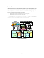
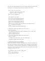
AIM project team has been developing the model for assessing the future environmental loads based
on the past socio-economic trends and future scenarios. By using this model, the environmental
trends through 2032 in the Asia-Pacific countries have been estimated. Following 2 types model
have been developed because of accessibility to data sources;
•
Model A: Based on IEA (International Energy Agency) energy data
•
Model B: Based on UN (United Nations) energy data
In the following sections in this document, we will introduce the structure of each model, and
describe how to use this model to prospect the future environmental trends.
Scenario generation & AIM/Trend
past economic trend
China India Korea Japan
Thailand
Discussion
past environmental
trend
Input
Renewable Energy
energy
AIMAIM/
TREND
Trend
Population growth
Growth
Economic Growth
growth
Output
Energy efficiency
Efficiency
Improvement
improvements
Narrative scenarios
Scenarios
Asian Quantitative
quantitative
Future
Scenarios
scenarios
economic trend
Fe
ed
ba
ck
Future
environmental trend
Future estimates
Estimates
Future
economic trend
Future
environmental trend
Concept of AIM/Trend model
-3-
2. Model structure
2.1 Model A
2.1.1 Overview
Model A covers the countries that have the IEA energy balance table. Model B is used for the
countries that do not have the IEA energy balance table.
2.1.2 Covered countries
Model A covers the following 25 countries;
South Asia: Bangladesh, India, Iran, Sri Lanka, Nepal, Pakistan
South East Asia: Indonesia, Myanmar, Malaysia, Philippines, Singapore, Thailand, Vietnam
East Asia: China, Japan, Korea,Rep, Korea,Dem, Taiwan
Central Asia: Kazakhstan, Kyrgyz Republic, Tajikistan, Turkmenistan, Uzbekistan
South Pacific: Australia, New Zealand
Regression
Assumption
Regression
Assumption
Driving Force
Population
GDP
*IVASHR
*AVASHR
*PFCSHR
CARCAP
Elasticity
IND: IVA
TPR: CAR
TPO: GDP
AGR: AVA
OTH: PFC
AEEI
Final Energy Demand
Regression
IND, TPR, TPO, AGR, OTH Assumption
Electricity Share
Heat Share
IND, TPR, TPO, AGR, OTH
Final Energy Demand:
Final Energy Demand:
Electricity and Heat
excluding Electricity and Heat
IND, TPR, TPO, AGR, OTH
IND, TPR, TPO, AGR, OTH
Assumed generation
Assumed share
Efficiency
Assumed share
efficiency
Scenario
Primary Energy Supply
Input for Electricity plant,
COL, OIL, GAS, CRW
Heat plant, and CHP
NUC, HYD, GEO, NEW
IND: Industry
TPR: Road transport
TPO: Other transport
AGR: Agriculture
OTH: Other
IVA: Industry Value Added
AVA: Agriculture Value Added
PFC: Private Final Consumption
CARCAP: Car numbers per capita
COL: Coal
NUC: Nuclear
CRW: Combustible HYD: Hydro power
and renewables GEO: Geothermal
NEW: Wind, PV, and so on
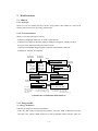
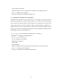
Calculation flow of detailed data model (Model A)
2.1.3 Energy module
(1) Energy classification
Following 10 energies are treated in this Model A;
COL (coal), OIL (crude oil and petroleum products), GAS (gas), CRW (combustible renewables
and waste), NUC (nuclear), HYD (hydro power), GEO (geothermal), NEW (wind, PV, and so on),
-4-
HET (heat), and ELE (electricity).
(2) Economic sectors
Energy conversion sector has following 5 sub-sectors;
ELP (power generation), HTP (heat supply system), CHP (combined heat and power plant), DST
(distribution of energy), and TFM (transformation). The final energy demand sector has following
6 sectors: IND (industry), TPR (transport on road), TPO (other transport), AGR (agriculture),
OTH (other), and NEU (non-energy use).
(3) Estimation of final energy demand
Final energy demand except NEU is described as the function of driving force (DRV). Driving force
of IND, TPR, TPO, AGR, and OTH is basically defined as industrial value-added (IVA), numbers of
car (CAR), GDP, agricultural value-added (AVA) and private final consumption expenditure (PFC),
respectively. Elasticity between each final energy demand and driving force is calculated by
regression analysis using historical data. If these data are not available, GDP can be used for the
driving force. Following equation is assumed:
TFE i (t ) = Ai (t ) × TFE i (t 0 ) × {DRV i (t ) / DRVi (t 0 )}
ELS i
Ai (t ) = (1 − AEEI i (t ) / 100) (t −t0 )
where,
TFE i (t ) : total final energy demand for sector i , time period t
DRV i (t ) : driving force for sector i, time period t
ELS i : elasticity for sector i
AEEI i (t ) : autonomous energy efficiency improvement for sector i, time period t
i : final energy demand sector, i ={IND,TPR,TPO,AGR, OTH}
t : simulation time period, t0: initial time period
NEU (Non-energy use demand) is estimated from the following equations. It is assumed that NEU
consists of oil based on historical data.
NEU (t ) = FE IND ,OIL (t ) /FE IND ,OIL (t 0 ) × NEU (t 0 )
where,
FE i , e (t ) : final energy demand for sector i , energy e , time period t
e : energy, e ={OIL, COL, GAS, CRW, NUC, HYD, GEO, NEW, ELC, HET}
(4) Estimation of future driving force
To estimate the trajectory of driving force (IND, TPR, TPO, AGR, and OTH), IVASHR (GDP share
-5-
of IVA), CARCPT (car numbers per capita), PFCSHR (GDP share of PFC), and AVASHR (GDP
share of AVA) are estimated from regression analysis using GDP per capita for independent
variables. To estimate IVASHR in other way SVASHR (GDP share of SVA (service value added) is
also estimated.
(5) Share of energy in final energy demand
Final energy demand consists of electricity, heat, and others.
a) Share of electricity: The share of electricity in each final energy sector is estimated by using the
regression analysis using driving force for independent variable.
b) Share of heat: The share of heat in each sector is fixed at that in the latest year for which data are
available in all sectors.
c) Share of other energy: The share of fossil fuel energy is estimated by using the regression analysis
using driving force for independent variable.
(6) Fuel share and energy efficiency in energy conversion sector
CHP and HTP are only used in specific countries in Asia-Pacific region. Share of fuel input into
HTP and share of fossil fuel input into CHP are assumed to be constant. Share of fossil fuel input
into ELP is calculated by regression analysis. Non-fossil fuel input into CHP and ELP are depended
on scenario assumption.
The electricity generation efficiency of ELP and CHP with COL, OIL, GAS, and CRW is assumed
by using exogenous energy efficiency improvement parameter. The generation efficiency of NUC,
HYD, GEO, and NEW are fixed as per IEA’s definitions (NUC: 0.33, HYD: 1.0, GEO. 0.1, NEW:
0.1). The heat generation efficiency is assumed to be fixed as that in initial simulation period.
(7) Total primary energy supply
Primary energy supply is calculated with final energy demand, energy conversion process, and
distribution loss. Distribution loss of fossil fuel, electricity, and heat is assumed to be constant as that
in initial simulation period.
(8) CO2/NOX/ SOX/CH4/N2O/CO emissions
Energy related GHG emissions are calculated by simulation result and assumed emission factor.
NOX and SOX emissions are assumed to be reduced according to increase of GDP per capita, known
as Kuznets curve.
2.1.4 Water module
(1) Model Features
Estimated variables:
-6-
ƒ Domestic water withdrawal
ƒ Industrial water withdrawal
ƒ Agricultural water withdrawal
ƒ Domestic water consumption
ƒ Industrial water consumption
ƒ Agricultural water consumption
Driving forces (explanatory variables) of future water withdrawal
ƒ Population (Historical trend and projection)
ƒ GDP (Historical trend and projection)
ƒ Share of industrial value added (Projection)
ƒ Urban and rural population supplied water service
ƒ Urbanization ratio (Historical trend and projection)
ƒ Irrigated area (Historical trend)
ƒ Current amount of water withdrawal in domestic, industrial and agricultural sectors
Assumptions of parameters related with technology improvement
ƒ Annual ratio of water use efficiency improvement in domestic sector
ƒ Annual ratio of water use efficiency improvement in industrial sector
ƒ Annual ratio of water use efficiency improvement in agricultural sector
(2) Domestic water withdrawal and consumption
Domestic water withdrawal is assumed to change proportionally to population that has access to
water supply service (water-supplied population). Since water-saving technology is expected to
improve in future in domestic sector, future change of water-use efficiency is assumed exogenously
and multiplied by the withdrawal estimated from the change of water-supplied population.
Water-supplied population is projected for urban and rural areas separately. The current tendency of
water-supplied population change is considered to continue in future with saturation. Based on the
water-supplied population in 1980 and 1990, trend of water-supplied population change is decided.
For countries where ratio of water-supplied population (water-supplied population / total population)
in 1990 is higher than that in 1980, it is assumed that the ratio of water-supplied population will
continue to increase at the same pace. Then the increased ratio is multiplied to the future population
projected by the World Bank in order to estimate water-supplied population. This assumption stands
on the consideration that quality of life will continue to improve if enough resource (in this case,
water resource) is available.
On the other hand, for the country where ratio of water-supplied population decreased during
1980s, it is assumed that the water-supplied population (not the rate) will change at the same pace.
Usually water-supplied population still increases (reflecting population increase) even in the nation
-7-
where ratio of water-supplied population decreases. This assumption stands on the consideration that
decreasing ratio of water-supplied population reflects the availability of water resources.
WDOM (t) = WDOM, URB (t) + WDOM, RUR(t)
= WDOM(1990) / ( WSPURB (1990) + WSPRUR(1990) )
* (WSPURB (t) + WSPRUR(t) ) * AWEIDOM(t)
WDOMC (t) = WDOM (t) *RCONDOM (t)
WDOM(t): Domestic water demand
WDOM, URB(t): Domestic water demand in urban area
WDOM, RUR(t): Domestic water demand in rural area
WSPURB(t): Water-supplied population in urban area
WSPRUR(t): Water-supplied population in rural area
AWEIDOM(t): Water use efficiency improvement in domestic sector compared with 1990
WDOMC (t) : Domestic water consumption
RCONDOM (t): Domestic water demand/consumption ratio
if
WSPURB(1990) / POPURB(1990) - WSPURB(1980) / POPURB(1980) > 0
WSPURB(1990)=POPURB(t)
* min(1,[WSPURB(1990)/POPURB(1990) -WSPURB(1980)/POPURB(1980)]) / 10years*(t-1990)
POPURB(t): Population in urban area
POPRUR(t): Population in rural area
if
WSPURB(1990) / POPURB(1990) - WSPURB(1980) / POPURB(1980) < 0
WSPURB(t) = min(A,B)
A = (WSPURB(1990) - WSPURB(1980)) / 10*(t-1990) + WSPURB(1990)
B = POPURB(t) *( WSPURB(1990) / POPURB(1990) )
(3) Industrial water withdrawal and consumption
Industrial water withdrawal is assumed to change proportionally to industrial value added (IVA).
Since water-saving technology is expected to improve in future in industrial sector, future change of
water-use efficiency is assumed exogenously and multiplied by the withdrawal estimated from the
change of IVA. In order to project the IVA in future, the time-series trend of the share of IVA in GDP
is multiplied by the GDP of the scenario.
WIND(t)=W(1990) * ( IVA(t) / IVA(1990) ) * AWEIIND(1990)
WINDC (t) = WIND (t) *RCONIND (t)
WIND(t): Industrial water demand
-8-
IVA(t): Industrial value added
AWEIIND(t): Water use efficiency improvement in industrial sector compared with 1990
WINDC (t) : Industrial water consumption
RCONIND (t): Industrial water demand/consumption ratio
(4) Agricultural water withdrawal and consumption
Agricultural water withdrawal is closely related to the size of irrigated area. Since critical factors
which govern irrigated area are different among countries, it is not easy to project future irrigated
area by multi-factor regression approach. In this example, however, irrigated area is projected as the
function regressed with two factors (logarithm of GDP per capita, logarithm of population) as a
simplified method. For more realistic projection, factors used for regression should be selected
separately for each country considering its background. For future population and GDP, projection
by World Bank is derived from the database file.
WAGR(t) = WAGR (1990) * (IRGAREA(t) / IRGAREA(1990) ) * AWEIAGR(t)
IRGAREA(t) = F (log(POP(t)), log(GDP(t)/POP(t)) )
WAGRC (t) = WAGR (t) *RCONAGR (t)
WAGR(t): Agricultural water demand
IRGAREA(t): Irrigated area
GDP(t): GDP
POP(t): Population
AWEIAGR(t): Water use efficiency improvement in agricultural sector compared with 1990
WAGRC (t) : Agricultural water consumption
RCONAGR (t): Agricultural water demand/consumption ratio
-9-
2.2 Model B
(1) Overview
For the several countries, for which IEA energy statistics data are not available, Model B is
constructed for estimation of environmental loads in the future.
(2) Covered countries
Model B covers following 17 countries;
South Asia: Afghanistan, Bhutan, Maldives
South East Asia: Brunei, Cambodia, Laos
East Asia: Mongolia
Central Asia: Kazakhstan, Kyrgyz Republic, Tajikistan, Turkmenistan, Uzbekistan
South Pacific: Fiji, Kiribati, Nauru, Palau, Papua New Guinea, French Polynesia, Solomon Islands,
Tonga, Vanuatu, Samoa
(3) Energy data
•UN Energy Statistical Yearbook 2000 is used.
a) Consumption of Commercial Energy (Liquids, Solids, and Gas)
*1
b) Consumption of Commercial Energy (Electricity)
*2
c) Consumption of Commercial Energy (Total)
*3
*1: “Liquids, Solids, and Gas” correspond to OIL, COL, and GAS in Model A respectively.
*2: Electiricity = (Electricity from geothermal, hydro, nuclear, solar, tide, wind and wave) +
imports - exports.
*3: Total = Liquids + Solids + Gas + Electricity
In “UN Energy Statistical Yearbook 2000”, *3 is the same as the total primary energy supply
in IEA Energy Balance Table (“Statistical Yearbook”, ”Energy Statistics Yearbook”).
So we use the phrase “Total Primary Energy Supply (TPES)” for “Total Consumption of
Commercial Energy (CCE)”.
The share of the each energy is fixed as that in 1995.
(4) Primary energy supply
Energies are categorized as Liquids, Solids, Gas, Electricity and Traditional fuelwood. Liquids,
Solids, and Gas correspond to OIL, COL, and GAS in Model A respectively. Electricity (ELC)
consists of supply from geothermal, hydro, nuclear, solar, tide, wind, wave, import, and export.
Traditional fuelwood (TRF) corresponds to CRW in Model A. Each energy supply is assumed to be
decided by GDP and AEEI.
This can be given by the following equation:
- 10 -
PE e (t ) = Ae (t ) × PE e (t 0 ) × {GDP(t ) /GDP (t 0 )}
Ae (t ) = (1 − AEEI e (t ) / 100) (t −t0 )
PEe (t ) : primary energy supply for energy e , time period t
GDP (t ) : GDP, time period t
AEEI e (t ) : autonomous energy efficiency improvement for energy e , time period t
e : energy, e ={OIL, COL, GAS, ELC, TRF}
t : simulation time period, t0: initial time period
(5) Emission Factors
Emission factors of NOX and SO2 are calculated from following way;
a) Case of no information on total emissions
The numbers of the emission factors are estimated based on “Greenhouse Gas Inventory
Reference Manual” from IPCC.
b) Case of available information on past emissions
The numbers of emission factors of SOX and NOX are calculated by using the latest emission data.
The changes of the numbers of emission factors in the future, and the definition of CO2 emission
factors are the same as Model A.
- 11 -
3. How to use Models
3.1 Installation of AIM/Trend Model
a) Installation of AIM/Trend Add-In
At the beginning AIM/Trend Add-In should be installed on your computer. Please refer to
“AIM/Trend Add-In Manual” for installation of this Add-In for more detailed information.
b) Installation of AIM/Trend Models
Please copy the directory “¥AIMTrend” in the CD-ROM to your computer.
3.2 Model A
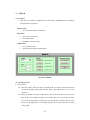
(1) File Open
Open the excel workbook “Model A.xls” in the directory ¥AIMTrend. In this workbook, following
sheets have been prepared.
Interface sheet
•
GUI: operational sheet for calculation.
Data sheets
•
Hst: past data except energy balance data.
•
Bal: energy balance data.
•
Pam: future scenario data.
•
Ene-trend: future energy scenario data calculated by past trend.
•
Ene-user: future energy scenario data set by the user.
•
Ene: future energy scenario data used for projection.
•
Emf: emission factor for GHG emissions.
•
WatPam: future water scenario data.
Output sheets
•
GPro: projection figures of main indexes.
•
Pro: projections related to energy.
- 12 -
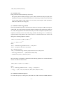
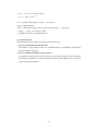
GUI of Model A
(2) Operation of GUI
1) File operation
z Select the country, which you want to calculate, and write down the case name on the
“case” blanket. You can choose from 5 scenarios (REF, MF, PR, FW, GT) and your
scenarios. When you want to refresh the data, please push “Reload” button. The default
data are set on each worksheet.
z When you change several data on data sheets, you can save those data. If you write case
name on the “save” blanket and push “Save” button, data set are saved with case name.
You can see the data again by writing case name and pushing “Reload” button. If you do
not write anything on the “case” blanket and push “Save” button, data are saved in “Temp”
folder.
z UNEP published GEO-3: Global Environment Outlook 3 (UNEP 2002) before
Johannesburg Summit and prepared following 4 scenarios: Market First scenario (MF),
Policy First scenario (PR), Security First scenario (FW), and Sustainability First scenario
(GT). The Market First scenario envisages a world in which market-driven developments
- 13 -
coverage on the values and expectations that prevail in industrialized countries; In the
Policy First world, strong actions are undertaken by governments in an attempt to reach
specific social and environmental goals; The Security First scenario assumes a world of
great disparities, where inequality and conflict prevail, brought about by socio-economic
and environmental stresses; and Sustainability First pictures a world in which a new
development paradigm emerges in response to the challenge of sustainability, supported by
new, more equitable values and institutions.
2) Future projection
z If you want to calculate future projections related to energy use, please push “Projection of
Energy and Emission” button. If you want to calculate future projections related to water
use, please push “Projection of Water Use” button. After that please push “Write Output to
"Result" Sheet” button to write out the results. The worksheets, “GPro” and “Pro” will
show the results related to energy, emissions and water results that are reflected by latest
data change. You can calculate above procedures with “Projection all” button.
3) Future Parameter
z Future parameter can set as following processes;
On “Pam” sheet
¾ User sets population and GDP scenario.
¾ Driving force will be projected with “Projection of Driving Force” button.
¾ User can modify scenario by overwriting “#table Drv” on Pam sheet.
¾ User can modify scenario by overwriting “#table ELS”, and “#table AEEI”. Final
energy demand will be projected with “Projection of Final Energy Demand” button.
User can also modify “#table FE” directly on Pam sheet.
On “Ene-user” sheet
¾ Energy share will be projected with “Projection of Energy Share” button.
¾ User can modify energy share scenario by overwriting each table on “Ene-user” sheet.
¾ User can modify other energy scenario by overwriting each table on “Ene-user” sheet.
¾ The button “Energy related Parameter Setting” will set energy scenario. This process
combines “Ene-user” sheet and “Ene-trend” sheet into “Ene” sheet.
z The button “Pam Set All” will set all parameters following model calculation.
4) Worksheet operation
z If you push the button “show program sheets”, the worksheets will be shown.
z “ATML” controls the GUI program and has the country code.
z “P-Eng” has the program to prospect energy related scenario. “P-Wat” has the program to
- 14 -
prospect water related scenario. “P-GHG” has the program to calculate GHG emissions.
“WATPAM” is the worksheet for selecting data related to water projection.
z “index” has the codes which are used in each program.
z Each program is written in ATPL.
z If you push the button “hide program sheets.”, the above worksheets will be hidden
z If you push the button “delete temporal sheets”, the temporal worksheets will be deleted.
(3) Scenario setting
The worksheets “Pam” and “Ene” have the important assumptions data about economy, energy, and
emissions. If there are blank data on the table, they are interpolated at calculation.
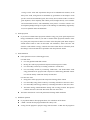
Table Scenario variable of Model A
Name of variable
Type of
Descriptions
variable
Table
POP
Time Series
Population (1000)
Basic
GDP_R
Time Series
Economic growth rate (%/year)
Basic
AEEI.I
Time Series
AEEI (%/year)
AEEI
Time Series
TPES (kTOE)
SUP.NFOS
I={IND, TPR, TPO,
AGR, OTH}
TPS.SUP.J
J={NUC, HYD, GEO,
NEW, ELE, HET}
ELE.ELP.CRW
Time Series
Electricity supply by CRW power plant
SE.CRW
(kTOE)
ELE.CHP.TOT
Time Series
Electricity supply by CHP plant (kTOE)
ELE.CHP.TOT
ELP.SHR.J
Time Series
Share of fossil fuel power plant in total
fossil fuel power plant ( %)
SHR.ELP.FOS
J={COL, OIL, GAS}
•J (ELP.SHR.J) = 1
ELP.IMP.J
Time Series
J={COL, OIL, GAS, CRW}
Improvement rate of generation efficiency
for fossil fuel and CRW power plant
ELP.IMP
(%/year)
ELP.MXEFF.J
J={COL, OIL, GAS, CRW}
EMS.EMF.J.L
Time Series
Parameter
J={COL, OIL, GAS, CRW}
Maximum efficiency of generation
efficiency for fossil fuel and CRW power
plant (%)
Initial value of NOx, SO2 emission factors
ELP.MXEFF
GHG1
(Gg-NOx/kTOE, Gg-SO2/kTOE)
L={NOX, SO2}
EMS.RDPNT.M.L
M={P1, P2}
L={NOX, SO2}
Parameter
When GDP per capita is achieved at this
point, emission factor is stating to reduce.
(1000US$)
- 15 -
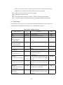
GHG1
Name of variable
EMS.MXFCT.L.M
Type of
Parameter
L={NOX, SO2}
M={P1, P2}
EMS.RDR.M.L
Descriptions
variable
Emission
factor
>=
EMS.EMF.J.L
Table
*
GHG1
EMS.MXFCT.L.M.
Parameter
Reduction rate of emission factors (%/year)
GHG1
L={NOX, SO2}
M={P1, P2}
URAT
Time Series
Urbanization rate (%)
Urat-m
AWEI.I
Time Series
AWEI (%/year)
AWEI
I={IND, AGR, DOM}
- 16 -
3.3 Model B
(1) File Open
ƒ Open the excel workbook “Model B.xls” in the directory ¥AIMTrend. In this workbook,
following sheets are prepared.
Interface sheet
•
GUI: operational sheet for calculation.
Data sheets
•
Pam: future scenario data.
•
Hst: historical data.
•
PERIOD: set for time period
Output sheets
•
Pro: projection results.
•
GPro: projection figures of main indexes.
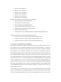
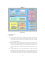
Fig. GUI of Model B
(2) Operation of GUI
1) File operation
z Select the country, which you want to consider. When you want to refresh the data those
you already changed, please push “Reload” button. The default data are set on each
worksheet.
z When you change several data on data sheets, you can save those data. If you write case
name on the “case” blanket and push “Save” button, data set are saved with case name.
You can see the data again by writing case name and pushing “Load data” button. If you
do not write anything on the “case” blanket and push “Save” button, the data are saved in
“temp” folder.
- 17 -
2) Future projection
z Please push “Project” button on the sheet “GUI” to start projection.
3) Worksheet operation
z If you push the button “show program sheets”, the worksheets, “ATMC”, “index”, “P-Pro”,
“INDEX”, and “PERIOD” will be shown.
z If you push the button “hide program sheets”, the above worksheets will be hidden
z If you push the button “delete temporary sheets”, the worksheets “Wrk”, which are used for
calculation, will be deleted.
(3) Scenario setting
Table Scenario variable of Model B
Name of Variable
Type of variable
Descriptions
POP
Time series
Population (1000)
GDP_R
Time series
AEEI
Time series
Economic
growth
(%/year)
AEEI (%/year)
- 18 -
Table name
DRV
rate
DRV
AEEI