1
Terms and Conditions of Use:
this document downloaded from
vulcanhammer.net
Since 1997, your complete
online resource for
information geotecnical
engineering and deep
foundations:
The Wave Equation Page for
Piling
Online books on all aspects of
soil mechanics, foundations and
marine construction
Free general engineering and
geotechnical software
All of the information, data and computer software
(“information”) presented on this web site is for general
information only. While every effort will be made to insure
its accuracy, this information should not be used or relied on
for any specific application without independent, competent
professional examination and verification of its accuracy,
suitability and applicability by a licensed professional. Anyone
making use of this information does so at his or her own risk
and assumes any and all liability resulting from such use.
The entire risk as to quality or usability of the information
contained within is with the reader. In no event will this web
page or webmaster be held liable, nor does this web page
or its webmaster provide insurance against liability, for
any damages including lost profits, lost savings or any
other incidental or consequential damages arising from
the use or inability to use the information contained
within.
This site is not an official site of Prentice-Hall,
Pile Buck, the University of Tennessee at
Chattanooga, or Vulcan Foundation
Equipment. All references to sources of
software, equipment, parts, service
or repairs do not constitute an
endorsement.
And much more...
Visit our
companion site
http://www.vulcanhammer.org
Final Report
THREE DIMENSIONAL FINITE ELEMENT PROGRAM TO PREDICT
THE BEHAVIOR OF SOILS AND SUBSTRUCTURE COMPONENTS
State Project No.: 99700-3583-119
UF Project No.: 4910450460712
WPI No.: 0510834
Contract No.: BB-301
Submitted to:
Mr. Richard Long
Research Center
Florida Department of Transportation
605 Suwannee Street, MS 30
Tallahassee, FL 32399-0450
(904) 488-8572
Mr. Peter Lai, PE
Florida Department of Transportation
605 Suwannee Street, MS 5L
Tallahassee, FL 32399
(904) 488-8911
Michael McVay, Zafar Ahmad, Girish Bhanushali, Brian Basterrachea & Sayed Hashimi
Department of Civil and Coastal Engineering, College of Engineering
345 Weil Hall, P.O. Box 116580, Gainesville, FL 32611-6580
Tel: (352) 392-8697 SunCom: 622-8697 Fax: (352) 392-3394
May 2001
TABLE OF CONTENTS
page
LIST OF FIGURES ......................................................................................................... iii
CHAPTERS
1
INTRODUCTION ........................................................................................ 1
2
PlasFEM ....................................................................................................... 2
2.1
2.2
2.3
2.4
2.5
3
Introduction......................................................................................... 2
Geometry............................................................................................. 3
2.2.a One Dimensional ..................................................................... 3
2.2.b Two Dimensional .................................................................... 4
2.2.c Three Dimensional .................................................................. 4
2.2.d Interface Element .................................................................... 5
Modeling the Construction Process .................................................... 7
Constitutive Models ............................................................................ 9
2.4.a Linear Elastic........................................................................... 10
2.4.b Elastic Perfectly Plastic .......................................................... 10
2.4.c Elastic Perfectly Plastic (Curved Failure Surface ................... 11
2.4.d Elastic-Plastic, Sandler-DiMaggio .......................................... 12
2.4.e Elastic-Plastic, Cam-Clay........................................................ 13
2.4.f Elastic-Plastic, Sandler-DiMaggio with Creep ....................... 14
2.4.g Elastic-Plastic, Generalized Cam-Clay ................................... 15
2.4.h Nonlinear Elastic ..................................................................... 16
2.4.i Nonlinear Elastic-Modified Cam-Clay ................................... 17
2.4.j Nonlinear Elastic-Modified Cam-Clay with Creep................. 18
Modeling Consolidation...................................................................... 18
PlasGEN ....................................................................................................... 21
3.1
3.2
3.3
3.4
3.5
3.6
3.7
3.8
3.9
Introduction......................................................................................... 21
Main Screen ........................................................................................ 21
The “File” Drop Down Menu and Toolbar ......................................... 23
The “Edit” Drop Down Menu and Toolbar ........................................ 24
The “View” Drop Down Menu ........................................................... 25
The “Tools” Drop Down Menu and Toolbar ...................................... 27
Modeling the Construction Process or Events .................................... 39
Meshing and Creating PlasFEM File .................................................. 50
3.8.1 Quadrilateral Mesher................................................................. 51
3.8.2 Triangular Mesher..................................................................... 53
Zoom Feature ...................................................................................... 57
i
3.10 Modeling Consolidation...................................................................... 58
3.11 Editing by Right Clicking the Mouse in the Draw Screen.................. 61
4
PlasPLOT...................................................................................................... 65
4.1
4.2
4.3
4.4
4.5
5
Introduction – File Opening................................................................ 65
The “Options” Drop Down Menu and Toolbar .................................. 67
The “Results” Drop Down Menu and Toolbar ................................... 72
The “View” Drop Down Menu and Toolbar ...................................... 79
The “Window” Drop Down Menu...................................................... 85
EXAMPLES ................................................................................................. 90
5.1
5.2
5.3
5.4
Embankment Construction Over Soft Clay......................................... 90
Excavation Behind Soldier Pile Wall.................................................. 94
Culvert with Soil Embankment and Surface Load.............................. 96
Drilled Shaft Subject to Conventional Load Test ............................ 100
REFERENCES ............................................................................................................. 104
APPENDICES
A
PlasFEM – Input Manual (Version 2.4) ....................................................
Problem......................................................................................................
Coordinates ................................................................................................
Material......................................................................................................
Groups........................................................................................................
Boundary....................................................................................................
Initial..........................................................................................................
105
106
108
109
116
120
121
Events ........................................................................................................ 122
B
Notes on Material Models ......................................................................... 125
ii
LIST OF FIGURES
page
Figure
2.1
2.2
2.3
2.4
2.5
2.6
2.7
2.8
2.9
2.10
2.11
2.12
2.13
2.14
2.15
3.1
3.2
3.3
3.4
3.5
3.6
3.7
3.8
3.9
3.10
3.11
3.12
3.13
3.14
3.15
3.16
Variable 2 or 3 Node Truss Element ...............................................................
Variable 4 to 9 Node Plane Strain or Axisymmetric Element.........................
Six Node Plane Strain or Axisymmetric Element ...........................................
Variable 8 to 27 Hexahedral Brick Element....................................................
Six Node Interface Element.............................................................................
Event One ........................................................................................................
Embankment (Region 2) to be Placed in Event 2............................................
Placement of Surface Loading.........................................................................
Elastic Perfectly Plastic with Straight Failure Surface....................................
Elastic Perfectly Plastic-Curved Failure Surface ............................................
Sandler-DiMaggio Model (Elastic-Plastic) .....................................................
Yield Surface (i.e., Elastic vs. Plastic Strains) ................................................
Original Cam-Clay (Von Mises), GCC Model, and Mohr-Coulomb..............
Relation between Void Ratio and Mean Stress ...............................................
Modeling Consolidation with Boundary and Initial Conditions .....................
PlasGEN Main Screen View ...........................................................................
Drop Down Menu and Toolbar in PlasGEN ...................................................
“File” Drop Down Menu and Options.............................................................
“Edit” Drop Down Menu and Options ............................................................
“View” Drop Down Menu and Options ..........................................................
Color Chart for Customizing Line Work and Background Colors..................
“Tools” Drop Down Menu and Options..........................................................
Using Rectangle Option to Construct a Soil Layer .........................................
Use of the Quadrilateral (polygon) Option to Draw Upper Soil Layer...........
Use of the Quadrilateral Option to Draw the Planned Embankment ..............
Global Regions Created with Draw Feature....................................................
Global Regions Options ..................................................................................
Assigning Names to Each Global Region .......................................................
Assigning a Constitutive Model and Material Parameters to a Region ..........
“Support” Option in the “Tools” Drop Down Menu.......................................
Placing Pins, Vertical and Horizontal Deformation Restraint ........................
iii
3
4
5
6
6
7
8
9
10
11
12
13
15
16
19
22
23
24
25
25
26
27
28
29
30
30
31
31
32
33
34
LIST OF FIGURES--continued
Figure
3.17
3.18
3.19
3.20
3.21
3.22
3.23
3.24
3.25
3.26
3.27
3.28
3.29
3.30
3.31
3.32
3.33
3.34
3.35
3.36
3.37
3.38
3.39
3.40
3.41
3.42
3.43
3.44
3.45
3.46
3.47
3.48
4.1
4.2
4.3
4.4
4.5
page
Placing Vertical Rollers (Zero Lateral Movement) on Right Boundaries.......
Assigning Flow or Zero Pore Pressure at Boundary .......................................
Applying No Flow Conditions ........................................................................
Changing the Description of a Region ............................................................
“Undo” and “Redo” Options on the Drop Down Menu and Toolbar..............
Save the Problem as “example1” ....................................................................
Editing the “All Events”..................................................................................
New Event or Properties Popup Window........................................................
The Event Insitu and Associated Regions .......................................................
Remove a Region from the Insitu Event .........................................................
Active Regions for the Insitu State..................................................................
Adding the Embankment as the Second Event................................................
Two Events in “All Events” ............................................................................
Active Regions for Event Two ........................................................................
Applying a Surface Load.................................................................................
Event Three: Surface Load.............................................................................
Selecting Quadrilateral or Triangular Mesh....................................................
Selection of Quadrilateral or Triangular Mesher ............................................
Mesh Window with Options............................................................................
Quadrilateral Mesh and PlasFEM Data Set.....................................................
Triangular Mesh Properties .............................................................................
Triangular Mesh Popup Window ....................................................................
Identify the Exterior Boundary for Triangular Mesher ...................................
Triangular Mesh Generation ...........................................................................
Zooming in the Draw Screen...........................................................................
Translated Drawing Object..............................................................................
Inclusion of Water Table in Draw Screen .......................................................
Meshed Regions with Inclusion of Water Table .............................................
Right Clicking the Mouse Outside the Drawn Objects ...................................
Right Clicking the Mouse Inside a Region .....................................................
Right Clicking the Mouse at the Center of Any Boundary Line.....................
Properties Window for a Boundary.................................................................
PlasPLOT Opening Screen..............................................................................
Selecting a PlasPLOT file to View..................................................................
Embankment Problem Selected for Viewing ..................................................
Drop Down Menus and Toolbar......................................................................
Features of Drop Down Menu “Options”........................................................
iv
35
36
37
38
39
40
41
42
43
44
44
45
46
47
48
49
50
51
52
53
54
55
56
57
58
59
60
61
62
63
64
64
65
66
67
68
68
LIST OF FIGURES--continued
Figure
4.6
4.7
4.8
4.9
4.10
4.11
4.12
4.13
4.14
4.15
4.16
4.17
4.18
4.19
4.20
4.21
4.22
4.23
4.24
4.25
4.26
4.27
4.28
4.29
4.30
4.31
4.32
4.33
5.1
5.2
5.3
5.4
5.5
5.6
5.7
5.8
page
Plotting Node Numbers ...................................................................................
Turning On or Off the Drawing of Element Information................................
Displaying Only Insitu Soil without Embankment .........................................
Events Feature Under Options.........................................................................
Contour Option................................................................................................
Results Drop Down Menu ...............................................................................
Selection of Solid Displacement Results.........................................................
Contours of Vertical Displacement Under Embankment Construction ..........
Drop Down Menu with Stresses Identified .....................................................
Available Stresses to Plot with Time or Event................................................
Plot of Vertical Stress for Event Three ...........................................................
Plot of Vertical Stress for Event Three and 16 Colors ....................................
Selecting Pore Pressures to View ....................................................................
Pore Pressure Distribution and End of Construction.......................................
Changing Scale on Pore Pressure Distribution................................................
“View” Drop Down Menu in PlasPLOT.........................................................
Selection of Orientation and Size in Drop Down Menu “View” ....................
Selecting 10-Degree Rotation about Z-axis ....................................................
Zoom Option from Toolbar of Drop Down Menu: “View” ...........................
Zooming by One Hundred and Twenty-Five Percent .....................................
Translation Features in PlasPLOT ..................................................................
Translated Figure in the Viewing Area ...........................................................
Locating the Axes in the Drawing Frame........................................................
Locating the Origin at Center of Drawing Window........................................
“Window” Drop Down Menu in PlasPLOT....................................................
Multiple Windows for Displaying Results ......................................................
Multiple Views of Same Problem ...................................................................
Multiple Displays of Displacements and Stresses...........................................
Embankment Over Soft Clay...........................................................................
PlasPLOT View of Embankment ....................................................................
Embankment Displacement Results ................................................................
Embankment Vertical Stresses and Pore Pressure ..........................................
Excavation Behind Soldier-Pile Wall..............................................................
Excavation Behind a Soldier Pile Wall ...........................................................
Concrete Culvert with Embankment and Surface Loading.............................
Displacements of Soil and Culvert in Construction and with
Surface Load....................................................................................................
v
69
70
70
71
71
72
73
74
74
75
76
76
77
78
78
79
80
80
81
82
83
83
84
85
86
86
87
88
90
91
92
93
94
95
97
98
LIST OF FIGURES--continued
Figure
5.9
5.10
5.11
5.12
A.1
A.2
A.3
A.4
A.5
A.6
A.7
page
Vertical Stress in Soil and Culvert During Construction and
with Surface Load............................................................................................ 99
Drilled Shaft Founded in Clayey Silt .............................................................. 100
Vertical Displacement of Drilled Shaft and Surrounding Soil........................ 101
Shear and Vertical Stress in Soil Mass............................................................ 102
Failure Envelope for Drucker Prager Model (ismod=2) ................................ 110
Yield Surface of Cap Model (ismod=4) ......................................................... 111
Yield Surface of Cam Clay Model in p-q Space ............................................. 112
Octahedral Deviatoric Plane............................................................................ 113
Order of Connectivity for 2-3 Node Truss Element........................................ 117
Order of Connectivity: a) for 4-9 Node Element; b) for 8-27 Node
Hexahedral Brick Element ............................................................................. 118
Six-node Interface Element ............................................................................. 119
vi
CHAPTER 1
INTRODUCTION
The University of Florida’s Geotechnical Group has been developing a one, two
and three dimensional finite element code for modeling general Geotechnical problems
for the past eight years (1992-2000). Of interest is the ability to model the construction
process, either embankment construction, or excavation, as well as the application of
surface loads (tractions). Since many soils in Florida are saturated, it was important that
the program be capable of modeling both the solid phase and the fluid phase under both
static and dynamic loading. The outgrowth of this effort is the PlasFEM code.
Due to the significant amount of information required for input (i.e. nodal
coordinates, element connectivity, etc.) as well as voluminous output, a preprocessor
(PlasGEN) and postprocessor (PlasPLOT) have also been developed. This contract was
for the development of the preprocessor (PlasGEN). However, this report describes the
user input, features and capabilities of PlasGEN, PlasFEM, and PlasPLOT as well.
The computer system requirements for this suite of programs are a Pentium III
computer with at least a 500 Mz CPU, and 128 Mb of RAM. A readme file is provided
with the installation CD.
Chapter 2 describes the capabilities of PlasFEM, Chapter 3 gives PlasGEN
features, and Chapter 4 presents PlasPLOT’s capabilities. It is strongly suggested that
the user work along with the user manual when reading Chapters 3 and 4. The example
problems for these chapters are also provided on the installation CD. A line by line input
guide to PlasFEM is also provided in Appendix A.
1
CHAPTER 2
PlasFEM
2.1 Introduction
PlasFEM is a finite element code developed to solve one, two, and threedimensional static, and dynamic multiphase problems. Developed from the theory of
mixtures, i.e., conservation of mass and momentum of the each phase, PlasFEM solves
the coupled relationship between the skeleton (soil, rock, or concrete) and the fluid phase.
Presently, the change in skeleton and fluid pressures, as well as fluid flow is computed
due to external loads. It does not solve Laplace’s equation for fluid flow due to hydraulic
gradients, pumping etc. resulting in changing phreatic surfaces. PlasFEM is capable of
analyzing a problem with both small and large deformation theories. A reference for the
latter is “Centrifugal and Numerical Evaluation of Preloading on Polk County Parkway,”
by McVay and Ahmed (1999).
In the case of the Dynamic problem, PlasFEM, uses coupled mixture theory to
solve the two-phase problems for both the fluid and skeleton response. It’s capable of
handling either compressible or incompressible fluid behavior. The user may select
either a u-u (skeleton displacement and velocities) or u-p-u (skeleton displacement, fluid
pore pressure and skeleton velocity) representation. A reference for the latter work is
“Coupled Finite Element Formulations for Dynamic Soil-Structure Interaction,” by Paulo
Pinto (1998).
PlasFEM is presently a fully implicit code for both static and dynamic analysis.
The latter ensures that the user may select any time step (small or large) for computing
results. Also, it employs a multitude of different constitutive models (elastic and elasto-
2
plastic) to represent the skeleton phase. Examples of the models are pressure sensitive
elastic models (linear and nonlinear), multiple invariant plastic models (Cam-Clay,
DiMaggio-Sandler, etc.), and creep models (visco-plastic). Presently, for all the models,
a tangent stiffness is generated, ensuring a quadratic rate of convergence for each load or
time step.
A discussion of problem geometry (1D, 2D, and 3D), modeling the construction
process, constitutive models, and the necessary boundary conditions for consolidation
follow.
2.2 GEOMETRY
2.2.a One Dimensional – PlasFEM has a variable two or three node truss
element as shown in Figure 2.1. Typical use would be characterizing reinforced earth or
one-dimensional settlement. The element allows the use of most of constitutive models.
Also available for the element are pore pressure degrees of freedom at its two end nodes.
η
3
2
1
Figure 2.1Variable 2 or 3 Node Truss Element
3
ξ
2.2.b Two Dimensional – Problems handled by PlasFEM fall into the class of
plane strain or axisymmetric in nature. Examples of plane strain are roadway or
embankment construction, as well as tunneling and excavation. Cases of an
axisymmetric problem are drilled shaft construction with axial loading, and circular
footings. Two different classes of isoparametric elements are available in the program
for these problems. The first is a variable four to nine node quadrilateral (Figure 2.2),
and the second is a six-node triangle element (Figure 2.3). Both have available pore
pressure nodes at the corners. Presently, PlasGEN (preprocessor) will automatically
generate the mesh for both types of two-dimensional elements.
η
4
8
1
7
3
9
6
ξ
2
5
Figure 2.2 Variable 4 to 9 Node Plane Strain or Axisymmetric Element
2.2.c Three Dimensional – For boundary value problems in which
displacements do not occur in a plane (i.e., plane strain), or with cylindrical problems
4
with variations in the hoop (theta) direction (i.e., not axisymmetric), the user has the
option of a full three
3
6
1
5
2
4
Figure 2.3 Six Node Plane Strain or Axisymmetric Element
dimensional analysis. Examples of the latter are lateral and torsional loading of drilled
shaft or pile group, and abutments. For these problems, PlasFEM has available a variable
8 to 27 node isoparametric solid element (Figure 2.4). In the case of two phases, i.e.,
solid skeleton and fluid phase, pore pressure nodes are available at each corner of the
element.
2.2.d Interface Element - For frictional interfaces, in which one element slides
relative to one another (Figure 2.5). The interface element which is of zero thickness
(Figure 2.5) allows the elements (one on top of another) to slide relative to one another if
the shear stress between them is overcome. The frictional resistance is a function of the
5
normal contact stress developed between the two elements. Examples of their use would
be modeling an interface between a geotextile or ground anchors and soil.
η
11
4
16
3
25
15
19
8
7
12
22
20
10
21
27
26
1
13
18
9
23
5
ξ
24
2
14
6
17
ζ
Figure 2.4 Variable 8 to 27 Hexahedral Brick Element
η
6
4
5
ξ
1
2
3
Figure 2.5 Six-Node Interface Element
6
2.3 MODELING THE CONSTRUCTION PROCESS
PlasFEM is capable of modeling multiple number of different event types: gravity
turn on, excavation, and surface traction (loading). Gravity turn on adds the body forces
associated with the insitu stresses in an existing soil mass or with the placement of an
embankment. Excavation removes the body forces (gravity) due to the removal of a soil
mass. Surface traction (loading) applies a distributed stress on the boundary of a region.
For any event, the user has the option of performing gravity turn on, excavation, or
applying a surface traction. The event may occur in one time step or multiple steps as
identified by the user. Examples of gravity turn on (insitu and embankment construction)
and the application of a surface traction follow.
Consider a clay layer, which is to have a sand embankment constructed on top
with a surface load to be applied later. Event one (Figure 2.6) turns on the body forces
(insitu stresses) associated with gravity. Note the vertical rollers on the side of region
signify no horizontal movement only vertical movement whereas the triangles ( pins)
allow no movement (horizontal or vertical). All outer edges or boundaries (i.e., pins and
Region 1 (Event 1)
Figure 2.6 Event One
7
rollers) must have constraints. Turning on gravity is a necessity when a nonlinear stress
dependent constitutive model is employed. The insitu stresses from gravity will ensure
that the correct stiffness and strength are available for the embankment construction and
later surcharge.
After the placement of the existing soil, an embankment (Figure 2.7) is placed on
top of it in event two. As identified earlier, each region or group, which is placed
(Region 2, Figure 2.7) has gravity (body forces) turned on which load the underling soil,
(Region one) resulting increased stresses and displacements.
Region 2 (Event 2)
Region 1 (Event 1)
Figure 2.7 Embankment (Region 2) to be Placed in Event 2.
Finally, Event 3 involves the placement of the stress surcharge on top of region 2
as shown in Figure 2.8. Again, the stresses and displacements of the underlying regions
(1 & 2) will increase as a result of this traction.
8
As shown in the above example, the user can model the following construction
processes: gravity turn on (i.e., placement of soil regions), and surface traction (i.e.,
loading). The other construction process that can be modeled is excavation, i.e., the
removal of a soil region. Example of the latter would be the removal of surcharge (i.e.,
after preloading), and milling or excavation of roadway material.
Event 3
Region 2 (Event 2)
Region 1 (Event 1)
Figure 2.8 Placement of Surface Loading
2.4 CONSTITUTIVE MODELS
A material’s constitutive model describes its stress-strain relationship. The latter
is of fundamental importance because it describes the material’s strength and stiffness.
PlasFEM has a number of models available that are simpler to the more sophisticated
ones, which may be used to describe soil, rock, concrete, etc. A discussion of each model
follows. The line by line input for each of the models is given in Appendix A.
9
2.4.a Linear Elastic - The simplest available constitutive model is Hooke’s law
for an isotropic (same properties in all directions) material. It requires only two
parameters, Young’s Modulus, E, and Poisson’s ratio, ν.
This model is good for
preliminary analysis and will converge for any load increment.
2.4.b Elastic Perfectly Plastic – The next more advanced model which includes
failure (Figure 2.9) is the Drucker Prager Model. The material is linear elastic until the
stress path hits the failure surface. The failure surface is described in invariant stress
space with second invariant of the deviatoric stress tensor, sqrt(J2), and first invariant of
the stress tensor, I1. In terms of triaxial loading, sqrt(J2) is equal to (σ1 - σ)/sqrt(3) and I1
is equal to the vertical stress plus twice the confining stress.
J2
θ
α
I1
Figure 2.9 Elastic Perfectly Plastic with Straight Failure Surface
10
The failure surface is defined as sqrt(J2)failure = α + θ I1 and is fixed in space (i.e., does not
move). The user inputs α and θ parameters. For instance, selecting α equal to zero with
a nonzero θ parameter would be representative of a sand. Whereas, setting θ equal to
zero and a nonzero α parameter would be representative of a saturated clay in a total
stress analysis. The stress-strain behavior below failure is represented with linear elastic
model with input parameters: Young’s Modulus, E, and Poisson’s Ratio, ν. For plane
strain conditions, the Mohr Coulomb strength (c, ϕ) in terms of α and θ are given as:
α = 3 c / sqrt(9+12tan2ϕ ) and θ = tanϕ / sqrt(9+12tan2ϕ )
(2.1)
2.4.c Elastic Perfectly Plastic (Curved Failure Surface) – Material is linear
elastic (isotropic) below a curved failure surface (Figure 2.10). Again, the failure surface
is fixed in space, i.e.
√J2 = α - γ exp(-β I1) + θ I1
√J2
Elastic
α
Failure Surface
I1
Figure 2.10 Elastic Perfectly Plastic- Curved Failure Surface
perfectly plastic. The curved failure surface is developed with the gamma, γ, term
(Figure 2.10). Examples of such a surface would be a sand under high normal stresses or
11
a partially saturated clay. The elastic behavior is described with a Young’s Modulus, E,
and Poisson’s Ratio, ν.
2.4.d Elastic-Plastic, Sandler-DiMaggio - This model has a fixed failure surface
and a hardening surface (elliptic cap), which moves with the stress path (Figure 2.11).
Compressive
Corner Region
J2
Failure Surface
√ J2 = α - γ exp(-β I1) + θ I1
2
2
J2 = [ (I1 - L) – (X - L) ]/R
2
Elliptic Cap
Tensile
Corner Region
Elastic
α
Tension Cutoff
T = I1
T
0
L1
X
I1
Figure 2.11 Sandler-DiMaggio Model (Elastic-Plastic)
This model will generate plastic strains prior to failure. The model is expressed with
either a straight or curved failure surface, a tension cutoff and a cap, which hardens based
on the volumetric strain. The tension cutoff may or may not exist depending on the value
of T that the user inputs (i.e., outside failure surface).
For the Sandler and DiMaggio, the growth of the elliptic cap (Fig. 2.11) is given by:
12
εvp = W [ 1 – e-DX ]
(2.2)
where εvp is the plastic volumetric strain (total volumetric strain minus elastic
volumetric strain). Note, when X (first invariant of stress, mean stress times 3) in Eq. 2.2
is large, the exponential term approaches zero, and the plastic volumetric strain, εvp,
approaches W. The parameter D determines how fast the plastic volumetric strain, εvp,
approaches the limiting value W. The total number of material parameters are W, D,
gamma, alpha, theta, T, E, and ν. This model has been successfully used on rock and
sand.
2.4.e Elastic-Plastic, Cam-Clay – was developed originally by Schofield and
Wroth from Imperial College. Figure 2.12 shows the elastic and plastic regions
(separated by yield surface) in p, q space.
q
M
Yield Surface
1
Plastic
Elastic
p
pc
Figure 2.12 Yield Surface (i.e., Elastic vs. Plastic Strains)
The ratio of shear to volumetric plastic strains (i.e., permanent strains) is controlled by
the parameter M. The magnitude of volumetric plastic (permanent) strain is given by the
13
hardening relationship which relates the incremental change in Pc (mean normal stress)
to the volumetric plastic strain increment, εvp, as
dPc /Pc = (1+e0) dεvp /(λ - κ )
(2.3)
where λ , and κ are material parameters. Plotting natural log of Pc versus the plastic
volumetric strain, εvp , will result in λ as the primary loading slope and κ as the
unloading reloading slope. Other parameters needed are the soil’s Elastic Bulk Modulus
and Poisson’s ratio. The model is typically used to characterize clays.
2.4.f Elastic-Plastic, Sandler-DiMaggio with Creep – Modification to the
original Sandler and DiMaggio Model (2.4.d) such that the plastic strain (permanent
strain) is a function of time. Known as a Perzena type visco-plastic model, the total
growth of the elliptic yield surface is (Fig. 2.11) is still given by Eq. 2.2. However, the
rate of plastic strain rate growth is given by
dεp/dt =λ (F/F0)N ∂F/∂σj
(2.4)
where λ is called the fluidity parameter, and the exponent, N, is the power constant. In
expression 2.4, F is equation describing the yield surface (Fig. 2.11), and ∂F/∂σj is
normal to the yield surface, which describes the direction of plastic strain. This model
has two more parameters: λ and N than the original Sandler DiMaggio model.
2.4.g Elastic-Plastic, Generalized Cam-Clay (GCC) – Has the same shape and
hardening (growth of plastic volumetric strain) as the original Cam-Clay model (2.4.e) in
14
p-q space (Figure 2.12). However in the octahedral space (Figure 2.13), instead of being
a circle (original Cam-Clay), the yield surface is an ellipse.
σ
1
von Misces
Mohr-Coulomb
GCC Model
σ3
σ2
3
Figure 2.13 Original Cam-Clay (Von Mises), GCC Model, and Mohr-Coulomb
The shape of the GCC model in octahedral space, is controlled by the elliptic parameter
e. To match the Mohr-Coulomb, e should be selected such that
e = (3 - sinφ)/(3 + sinφ)
(2.5)
where e is limited between 0.5 and 2.0
2.4.h Nonlinear Elastic- generally referred to as a hyperelastic formulation.
This model has a nonlinear relationship between stress and elastic strain (recoverable
strain or deformation). The latter is due to the pressure sensitive relationship between
15
Bulk Modulus, K [E/3(1-2υ)] and Shear Modulus, G [E/2(1+υ)] with the mean stress, P
as follows:
G = G0 + (α/β) P and K = (P0/κ) β exp [ (εve - εv0e )/ κ ]
(2.6)
β = 1 + 3α (εse)2 / 2κ
(2.7)
Where
This Model is similar to the Duncan-Chang Model without a failure criterion.
Parameters required for the model are: α, G0, κ (see Figure 2.14), and εv0e
2.4.i Nonlinear Elastic-Modified Cam-Clay – has a yield surface separating
elastic from plastic strains similar to the original Cam-Clay Model (Figs. 2.12), but a
different hardening (i.e., growth of Pc vs. volumetric strains). The relationship between
void ratio (function of total volumetric strain) and mean stress is given in Figure 2.14.
λ
1+ e
κ
Logarithm P
Pc
Figure 2.14 Relation between Void Ratio and Mean Stress
This is similar to plotting the oedometer (consolidation) data (e vs log σv’). In the
case of K0 (coefficient of lateral earth pressure at rest) equal to one, then σv’ (vertical
effective stress) is equal to the lateral effective stresses, and P (mean effective normal
stress, Figure 2.14) would equal to σv’. In such a case Cc (Compression Index) is equal
16
to lambda, λ, and the Cr (Recompression Index) would be equal to κ. Note that this
model is nonlinear elastic, because the bulk modulus, is a function of the mean stress
(function of κ) beneath the precompression stress, Pc, (see yield surface in Figure 2.12
and Figure 2.14).
2.4.j Nonlinear Elastic-Modified Cam-Clay with Creep - This model uses the
same yield surface and hardening as 2.4.i described in Figure 2.12. However, in the case
of the hardening (Figure 2.14), a time is associated with its development as given in Eq.
2.3. This is expressed with the fluidity parameter, λ, and a power constant, N. The latter
model was used to model the Polk County Expressway.
2.5 MODELING CONSOLIDATION
In the case of a saturated soil with a low permeability, the application of a gravity
load (i.e., embankment) or a surface traction (stress) will result in the development of
excess pore pressure above its hydrostatic value. PlasFEM solves for the resulting
effective stresses, deformations, and pore pressures (total values, i.e., excess plus
hydrostatic) as a function of time. Since, its solution is coupled (solving both
conservation of mass and momentum of individual phases), then usually both the total
stresses and pore pressure will change as a function of time.
In order for PlasFEM to solve such a problem, both initial conditions and
boundary conditions must be identified for the whole boundary. Consider the example
shown in Figure 2.15 as discussed earlier (Figure 2.8). To develop the correct insitu
stresses, the gravity load for the existing soil mass is turned on (Event 1). Event 2 is the
17
construction of an embankment over the existing soil and event 3 is the application of a
surcharge load. The boundary conditions for this problem are the deformation and flow
constraints. Pins and rollers given on the side and bottom of the existing soil mass
(region 1) describe the former. The flow constraint is shown by the
symbol in
Figure 2.15. It represents the flow of water out of boundary and is characterized with
zero pore pressure at that location. Note that on the sides and bottom of region 1 there is
no
symbol, which means that there is no flow at this location or that the boundary is
impervious. Also recognize that even though the water table is at the top of region 1,
that excess pore pressure may develop in region 2 due to its self-weight and the
application of the surface load (event 3). The latter is very much controlled by the
permeability of the region 2. An example of this is shown in chapter four’s Figures 4.19
and 4.20.
Event 3
Region 2 (Event 2)
Region 1 (Event 1)
Figure 2.15 Modeling Consolidation with Boundary and Initial Conditions
In the case of consolidation or dynamic loading, PlasFEM requires the user to
identify the permeability. Kij, the permeability matrix, defines fluid velocity in terms of
hydraulic gradient. The diagonal terms gives the velocity in terms of the three
18
orthogonal hydraulic gradients (in global X, Y, Z directions). The off diagonal terms are
the mixed contribution to the velocity from the other orthogonal hydraulic gradient terms.
Generally, for horizontal soil and rock layers, the off diagonal terms in Kij are zero. A
difference in the three diagonal terms would reflect a different fluid (water) velocity in
each direction for the same hydraulic gradient.
In the case of consolidation, the user must identify the time that each event
(Figure 2.15) is to occur over, as well the time that he/she wishes to view the results. The
latter is controlled by specifying the incremental time and the number of time steps in
PlasFEM. PlasFEM allows the user to stipulate different time increments for each event.
Specifics of the required time information is given in Appendix A which gives a line by
line input guide to the ASCII file required by PlasFEM.
19
CHAPTER THREE
PlasGEN
3.1 Introduction
PlasGEN is a preprocessor, which was developed to generate the ASCII input file
for PlasFEM (engine which performs the analysis). Since PlasFEM is a finite element
program, one of PlasGEN’s major functions is the generation of elements, nodal
coordinates, boundary constraints, and loading information for a user’s defined problem.
To allow the user’s efforts to focus on describing the geometry and material description,
instead of the meshing, etc., PlasGEN has two different automatic meshing
(quadrilaterals and triangles) routines. In addition, the user can easily add/delete events
(i.e., model construction: embankments, excavations, loads), as well as change material
models and properties, run analysis (PlasFEM) and view results (PlasPLOT) quickly
from PlasGEN’s toolbar. A description of PlasGEN’s input/use follows.
3.2 Main Screen
Shown in Figure 3.1 is the main screen of PlasGEN when opened from the
explorer window. This screen is broken into two smaller screens, a drop down menu list,
and a set of toolbar icons. The smaller screens within the main screen are adjustable by
positioning the mouse over their divider, left clicking and dragging the boundary left or
right. The screen on the right is the drawing paper in which the user creates his/her
problem (i.e., defines geometry, constraints, loading, etc.) of interest. The screen on the
left defines the event process. For instance, if the user wishes to start with an initial
20
Figure 3.1 PlasGEN Main Screen View
insitu soil profile (event 1), then build an embankment (event 2) followed by the
placement of a surface load (event 3), it would be described in the event window. The
construction of the user’s problem (geometry), boundary constraints, and loading is
readily available with the toolbar icons (Figure 3.2). However, as will be shown, most of
these features are also available in the drop down menus (Figure 3.2). A discussion of
both toolbar icons and drop down menus follows.
21
Open
an
Existing
Zoom
Create a New Problem
Run PlasPLOT
Surface Load
Water Table
Pin and Roller B.C.
Move Nodes
& Lines
File Save
Draw Polygon
Flow B.C.
Run PlaFEM
Material Model & properties
Draw Rectangle
Figure 3.2 Drop Down Menu and Toolbar in PlasGEN
3.3 The “File” Drop Down Menu and Toolbar
Shown in Figure 3.3 are the options available in the drop down menu “File”. The
first three options: “New”, “Open” and “Save” are identical to the first three icons on the
toolbar (Figure 3.2). When clicking “New”, whatever is displayed on the drawing screen
is lost along with the information in the event screen. The latter allows the user to start
over. The option “Open” allows the user to read a previously saved PlasGEN file (has
extension .gen) back into the preprocessor for editing, analysis, and display of output.
All PlasGEN files are saved with “Save” feature in the drop down menu option “File” or
its toolbar icon (Figure 3.2). The user specifies the name of the file without any
extension, and the program automatically assigns it the extension GEN. The specified
file name is also later used for the ASCI file that PlasGEN generates for PlasFEM (has
22
Figure 3.3 “File” Drop Down Menu and Options
extension: .dat). Similarly, the engine, PlasFEM, generates an output file with same
name (has extension: *.out, user may view with word processor), as well as PlasPLOT’s
input file (has extension *.prb not an ASCII file).
The “Print” option in the “File” drop down menu (Figure 3.3) prints a screen
capture of the image shown in the drawing screen. The “Print Setup” allows the user to
change printer, paper size, and figure orientation.
3.4 The “Edit” Drop Down Menu and Toolbar
The “Edit” drop down menu has three options (“Grid, “Snap to Grid” and “Clear
All”) as shown in Figure 3.4. The “Grid” option turns on a grid in the drawing screen
(right screen, see Figure 3.1). The latter is useful for laying out the problem. The “Snap
to Grid” option allows the user to slightly miss the node with the mouse when drawing
23
(i.e., holding the left mouse button down and moving mouse and then releasing mouse
button), but all nodes will snap to the nearest grid intersection (i.e., node).
Figure 3.4 “Edit” Drop Down Menu and Options
3.5 The “View” Drop Down Menu
Given in Figure 3.5 is the “View” Drop Down menu and associated options. The
first option is a toggle switch to turn on (check mark) or off (no check) the toolbar
Figure 3.5 “View” Drop Down Menu and Options
24
(Figure 3.2). The only advantage to turning off the toolbar is more drawing space. The
next option, “Status Bar” is a toggle to turn on (check mark) or off (no check mark) the
status bar on the bottom of the screen. The status bar (see Fig. 3.1) shows the coordinates
(x and y) of the mouse when in the problem drawing screen (right screen).
The “Events” option in the “View” drop down menu allows the user to toggle
between no event window (right screen Fig. 3.1) and an event window. One reason that
the user may temporarily decide to use this feature is for more drawing space for the
problem (right screen, see Fig 3.1).
The next option in the “View” drop down menu is the color option (Figure 3.5).
The latter is very useful for customizing the colors of the background, flow, support
condition, etc., in the drawing window. The user clicks on any from the list and a color
popup window (Figure 3.6) is shown, allowing the user to customize that feature’s color.
Figure 3.6 Color Chart for Customizing Line Work and Background Colors
25
The other two features in the “View” drop down menu are “Mesh” and “Mesher” which
create the finite element mesh (nodes, elements, etc.) and will be described later after the
geometry and boundary conditions are discussed.
3.6 The “Tools” Drop Down Menu and Toolbar
Shown in Figure 3.7 is the “Tools” drop down menu and options. Many of the
features available in this menu are also available in the toolbar as icons. For instance,
under option “Draw” (Fig. 3.7) is the rectangle and quadrilateral (polygon) shapes which
are available on the toolbar (Fig. 2.2) as icons. These latter two primitives are used to
construct all the regions, which make up the user’s problem. For instance, if the user
wished to construct an existing rectangular insitu soil mass, he/she would click this
option and construct it in the problem window (right side) using the mouse (Figure 3.8).
Figure 3.7 “Tools” Drop Down Menu and Options.
26
Figure 3.8 Using Rectangle Option to Construct a Soil Layer
If he/she wanted to construct another insitu layer on top they could use the quadrilateral
primitive as shown in Figure 3.9. Remember when using the quadrilateral (polygon)
option, the user is required to end (close) the polygon with the first node he/she drew.
Evident from Figure 3.9 is the extra two nodes on the top surface of the quadrilateral.
These two nodes will be the connecting points to add a planned embankment or soil
surcharge. In drawing any regions, the user must connect one region to another through
shared nodes (see Figure 3.9).
27
Figure 3.9 Use of the Quadrilateral (polygon) Option to Draw Upper Soil Layer
Shown in Figure 3.10 is the constructed embankment on top of the second upper soil
layer (Figure 3.9). Note each of the regions constructed in the draw screen shows up in
the events and regions screen on the left (Figure 3.9). To see them, simply double click
on the plus icon to the left of the “event and regions” title in the left screen. Figure 3.11
shows all the regions, which were created. The user has the option of renaming them
(i.e., region) by right clicking over each name. A popup window appears (Figure 3.12),
and user should select rename and type in a new name. To prevent confusion, the first
region drawn (i.e., bottom layer) is at the top of the event list followed by second, etc.
28
Figure 3.10 Use of the Quadrilateral Option to Draw the Planned Embankment
Figure 3.11 Global Regions Created with Draw Feature
29
Figure 3.12 Global Regions Options
Renaming the bottom region as clay, the next upper region as sand, and the top region as
embankment, the region name list should appear in the events and regions screen as
shown in Figure 3.13.
Figure 3.13 Assigning Names to Each Global Region
The user has the option of deleting any region by highlighting it in the Global
Regions list (left screen – Figure 3.12), right clicking the mouse, and selecting delete
from the popup window which appears (see Figure 3.12).
30
The user has the option of assigning a constitutive model and material properties
to each region by highlighting it in the Global Regions list (left screen – Figure 3.12),
right clicking the mouse, and selecting material from the popup window (see Figure 3.12)
which appears. A new popup window appears (Figure 3.14), and the user has a number
of different constitutive models to select based on the tab dialogue box.
Figure 3.14 Assigning a Constitutive Model and Material Parameters to a Region
Each tab’s constitutive model has its required material parameters displayed
below it. For instance, the linear elastic tab shows that the user needs to input both the
31
Young’s Modulus, and Poisson’s ratio for that region. Other parameters that would be
required for a fluid flow problem (consolidation), i.e., permeability coefficients would be
input at this time. After a constitutive model has been assigned to a particular region, its
symbol (LE) is shown next to each region in the “events and region” window (left screen
Fig. 3.13). Note the material constitutive model and its parameters for a given layer
(region) are also available from the toolbar icon “Materials”, shown in Figure 3.2. To
use the latter, just click on the icon and then click on the region in the draw view
window, Fig. 3.10.
Under the “Tools” Drop Down Menu is the “Support” condition option as shown
in Figure 3.15. The three choices are fixed (all three directions), horizontal roller (fixed
Figure 3.15 “Support” Option in the “Tools” Drop Down Menu
against movement in vertical direction) and vertical roller (fixed against movement in the
horizontal direction). All three options are available in the toolbar (see Figure 3.2). For
PlasFEM to run successfully, the user’s problem must be constrained against vertical and
32
horizontal movements at sufficient points along its boundaries to prevent rigid body
rotation. Generally, these locations are the bottom and the left and right boundaries. For
instance, selecting “Fixed” from the drop down menu or toolbar, and clicking with the
mouse on the bottom most region’s boundary results in Figure 3.16. A set of pins are
drawn which restrict that boundary movement to zero in both the x and y direction.
Figure 3.16 Placing Pins, Vertical and Horizontal Deformation Restraint
Next, add vertical rollers to the left and right boundaries of the bottom two
regions as shown in Figure 3.17. In order to accomplish the latter, the user must left click
at the center of each boundary’s edge for a total of four times. Note the display of
vertical rollers (i.e., y movement no x movement) differs from horizontal rollers
33
(i.e., y-movement, x-no movement). The vertical rollers are drawn as solids, and the
horizontal rollers are displayed as open circles.
Figure 3.17 Placing Vertical Rollers (Zero Lateral Movement) on Right Boundaries
The user can flip from pins (fixed, triangles, etc.) to rollers, by just left clicking again on
any boundary with the new constraint and it will be updated.
The next option in the “Tools” drop down menu is the “flow” option (Fig. 3.7),
which is also available on the toolbar (Fig. 3.2). After clicking on this feature (or icon),
the user needs to click on the center of a region’s boundary where there is flow, or zero
34
pore pressure. For instance clicking on the middle region’s top boundary, results in
Figure 3.18.
Figure 3.18 Assigning Flow or Zero Pore Pressure at Boundary
Note, to use this feature the events and region screen must have the “Global Regions”
heading (see left screen in Figure 3.18) highlighted. This is because the flow boundary,
and support constraint conditions apply to the global regions and not to a particular event
such as surface loading (discussed later). To undo the flow condition on a boundary, one
must click on the drop down icon next to the flow icon in the toolbar as shown in Figure
35
3.19. Note the default flow boundaries are no flow, and in the case of consolidation, the
user must have some boundaries that have flow in order for the water to escape.
Figure 3.19 Applying No Flow Conditions
The next option on the “Tools” drop down menu is “Materials” feature. Clicking
on this option activates the materials edit or assigns feature. The user needs to follow up
this action by left clicking his/her mouse on any of the displayed regions shown in the
drawing screen. The materials popup window as shown in Figure 3.14 is displayed for
that region.
For instance, if the user wished to change the Young’s Modulus for the
bottom region (clay) to 720,000 psf, position the mouse over this region, left click the
mouse and edit the modulus window as shown in Figure 3.20.
36
Figure 3.20 Changing the Description of a Region
The undo and redo features in the “Tools” drop down menu (Figure 3.21) are also
available in the toolbar as icons. Clicking on the undo will remove the last drawn object
in the draw screen whereas redo will place it back.
37
Figure 3.21 “Undo” and “Redo” options on the Drop Down Menu and Toolbar
It is important to save the file as the user builds his/her model. Clicking on the
“File” drop down menu and “Save As” feature, the following popup window (Figure
3.22) appears. Typing the name “example1” and clicking on save will generate a
PlasGEN file called “example1.gen”. Note the extension “.gen” is added to the file
name. PlasGEN will also generate a file named “example1.dat” when the user clicks on
the automatic mesh icon. Don’t do this yet, since all the necessary information for the
analysis has not been inserted into PlasGEN problem yet.
3.7 Modeling the Construction Process or Events
Once the geometry, constraints, and material description for the problem have
been defined (right screen Fig. 3.19), the construction process or events need to
38
Figure 3.22 Save the Problem as “example1”
be identified. The latter occurs in the events or regions screen (left side of Figs. 3.19 –
3.22). The user needs to first place the mouse on “All Events” and single click,
highlighting it. Next, right click the mouse and the popup screen as shown in Figure 3.23
appears. The options available are to create a new event, delete an event, delete a
region from an event, rename an event, and assign or edit the properties of an event.
As discussed earlier, this example is described by three events. The first event is the
39
placement of insitu soil (sand and clay layers) or a gravity turn on which results in the
initial stresses (i.e., Ko conditions).
Figure 3.23 Editing the “All Events”
The second event is the construction of the embankment or the gravity turn on of the
embankment soil and the third event would be the application of a surface load on top of
the embankment which was placed in event two.
To model the construction process, the original soil will be modeled by creating
an event called “insitu” by clicking on the “New Event” option in Figure 3.23 creating
popup window 3.24. This window controls the three types of events that PlasFEM will
analyze: 1) gravity turn on with the placement of a region (i.e., construction); 2) gravity
removal for a region due to excavation; and 3) surface traction or loading applied to the
top of a region. The user can only select one of these features under “Type” (right side
of popup – one of three different radio buttons: Gravity, Excavation, Surface Traction).
For this example, gravity was selected and the word “insitu” was typed into the name
slot. This name will later appear in the event description screen. In terms of gravity, the
40
only other information needed in this popup window is the No. of Time/Load steps
(found under General) and Total Time in the Gravity/Excav window. In the case of
water (i.e., saturated soil) the user must provide sufficient time for the insitu soil to reach
at rest conditions (1000 days etc.). Also, in the latter case where there is a lot of soil
placed, the user may wish to turn gravity on in multiple steps to assist PlasFEM in
convergence.
Figure 3.24 New Event or Properties Popup Window
Since this example has no water, one is sufficient for the number of steps and total time.
Clicking okay, and looking at “All Events” in the “Events and Regions” screen, Figure
3.25 is displayed. Note that all three regions have been assigned to event one (insitu)
41
Figure 3.25 The Event Insitu and Associated Regions
including the placement of the embankment. The latter is due to the fact that PlasGEN
assigns all regions to every newly created event. Consequently, the user needs to
highlight the embankment region (in events and regions screen) under the insitu event,
and left click the mouse. The popup window shown in Figure 3.26 is displayed.
42
Figure 3.26 Remove a Region from the Insitu Event
Clicking the “Delete Region” option will result in another popup window appearing
asking the user if they really want to do this. Clicking okay, and then double clicking on
insitu in the “events and regions” screen again results in Figure 3.27.
Figure 3.27 Active Regions for the Insitu State
43
Note by double clicking on “insitu” in the “event and regions” screen, the user is asking
PlasGEN to display the active regions for that event (green) in the drawing screen. Also,
note that the surface loading icon on the toolbar (Fig. 3.2) is now visible (Figure 3.27)
allowing the user to apply a surface load. Evident is that the boundary constraints (pins
and rollers) are not visible, since they are only displayed when the “Global Regions” are
highlighted in the “events and regions” screen (rights side of Figure 3.27).
In order to create event two the placement of the embankment, highlight “all
events” in the “events and regions” screen (left side of Figure 3.27) and right click the
mouse. Again, the “New Event” popup window (Fig. 3.23) will appear and the user
should select the “new event” option. The popup window, new event (Fig. 3.24) will
appear. Give the title as “embankment” and select the load type as gravity and the popup
windows should appear as Figure 3.28.
Figure 3.28 Adding the Embankment as the Second Event
44
Clicking on okay in the popup window (Figure 3.28) will create the second event.
Double click the mouse on “All Events” in the “events and regions” screen will now
show two events (Figure 3.29).
Figure 3.29 Two Events in “All Events”
Double clicking on “embankment” in the “events and regions” screen shows the active
regions in the draw screen window (Figure 3.30). Note all the regions (defined under
“Global Regions) are active or present for event two. Each is identified in the “events
and regions” window under the “embankment” event.
45
Figure 3.30 Active Regions for Event Two
Note also that the active regions are displayed in green. The user has the option of
applying surface traction on any boundary for this event.
The final event, is the placement of a surface load on top of the embankment,
which represents a roadway. This is accomplished by clicking on “All Events” in the
“events and regions” screen as shown in Figure 3.23. Next the new event popup window
appears (Figure 3.24). Specify “Surface Load” in the name box and click the radio
button “Surface Traction” in the Load Type section as shown in Fig. 3.31.
46
Figure 3.31 Applying a Surface Load
In the case of surface traction, the user needs to identify both the magnitude of the
surface traction, the number of steps and the beginning and ending time for the event.
The magnitude of the surface traction may be fixed over multiple time steps (stresses
may still change in body due to consolidation if saturated) or increase. For instance, if
the user specified 600 psf for step 1 and 6000 psf for step ten, then the event would
consist of ten steps with each step applying an additional 600 psf above the previous step.
The time increment in the event is established by taking the ending time minus the
47
beginning time and dividing by the number of steps. If the user wants to observe results
for a particular time, make sure their incremental times occurs at the times of interest.
Inputting the values shown in Figure 3.31 and clicking okay result in Figure 3.30.
Next click on the surface traction icon (Figure 3.2) in the toolbar and move the mouse in
the draw screen to the top boundary of the embankment region and left click the mouse.
A downward acting surface load (traction) Figure 3.32 is generated on top of the
embankment. If the wrong boundary is selected by mistake, the user may click on the
same boundary again, and the surface traction will be removed.
Figure 3.32 Event Three: Surface Load
48
3.8 Meshing and Creating PlasFEM File
Once the geometry, boundary, material description, events and loading have been
defined, the finite element mesh and PlasFEM file are ready to be created. The user has
two options for meshing, 9-node quadrilateral or 6-node triangular elements. In general
the 9-node quadrilateral element is more accurate, however, the 6-node triangular mesher
will mesh more irregular geometric shapes. It is suggested that the 9-node quadrilateral
be tried before the 6-node triangular mesher.
Either the quadrilateral or triangular mesher (both create PlasFEM files) is
available through the “View” Drop Down Menu. Figure 3.33 shows the “View” options
Figure 3.33 Selecting Quadrilateral or Triangular Mesh
with “Mesher” and “Properties” highlighted. The “Properties” option allows the user
to select the quadrilateral (see section 3.8.1) or triangular (see section 3.8.2) mesher as
well as control the fineness of the mesh (Figure 3.34). The default mesh is the 9-node
quadrilateral mesher.
49
Figure 3.34 Selection of Quadrilateral or Triangular Mesher
3.8.1 Quadrilateral Mesher is available under the “View” Drop down window and
“Mesher” > “Properties” option (Fig. 3.33). The user has the ability to coarsen or refine
the mesh through the “Mesh Grade” tab box (Fig. 3.34). To coarsen the mesh, select a
higher grid size (instead of 30 select 40, 50, 60, etc.), whereas to refine the mesh select a
lower grid size (i.e., 25, 20, 15, etc.). It should be noted that the 9-node quadrilateral
mesh has a fully quadratic description of displacements (i.e., shape functions) and a
coarser mesh may be used vs. a triangular mesh.
Once the type of mesher has been selected, the user selects the “mesh” option
from the drop down “View” menu (Figure 3.33). The latter automatically creates a new
window (Figure 3.35) displaying a copy of the geometry in the “draw screen”. The latter
50
window may be resized with the mouse to fit any portion of the screen, as well as
minimized or deleted. Right clicking the mouse in this window popups the available
Figure 3.35 Mesh Window with Options
options for the mesh window. Selecting “Mesh” invokes the mesher, which
automatically divides the geometry into quadrilaterals (Fig. 3.36), and writes out the
PlasFEM data file with the same name as identified earlier for PlasGEN (i.e., *.gen) but
with a different file type (i.e., *.dat). The user has the option of printing or clearing the
mesh (i.e., remove) from the same popup window.
Once, the mesh is successfully displayed on the mesh window, the user can now
analyze (lightning bolt) and view (plot) the results from the toolbar (Figure 3.2).
51
Figure 3.36 Quadrilateral Mesh and PlasFEM Data Set
3.8.2 Triangular Mesher - is available under the “View” Drop down window and
“Mesher” > “Properties” option (Fig. 3.34). The triangular mesher features (Figure 3.37)
that the user has control over are the minimum angles of the triangles in the mesh as
number of grid lines, horizontal and vertical that is used to construct the mesh.
52
Figure 3.37 Triangular Mesh Properties
Once the type of mesher has been selected, the user selects the “mesh” option
from the drop down “View” menu (Figure 3.33). The latter automatically creates a new
window displaying a copy of the geometry in the “draw screen”. Right clicking the
mouse in this window results in the popup windows shown in Figure 3.38. Evident from
this window, the user must specify both the exterior and interior boundary regions (i.e.,
each must close on itself). Selecting the exterior boundary, and left clicking with the
53
Figure 3.38 Triangular Mesh Popup Window
mouse on each line’s midpoint, as well traveling in a clockwise direction from line to line
results in Figure 3.39. In the case of an interior region (i.e., hole, etc. which isn’t to be
meshed), the user needs to left click with the mouse on each line in a counter clockwise
direction.
54
Figure 3.39 Identify the Exterior Boundary for Triangular Mesher
To create the triangular mesh, as well as the PlasFEM file (*.dat) with the
necessary data (elements, nodes, material description, etc.) click on mesh in the mesh’s
popup window (Fig. 3.38). The triangular mesh as shown in Figure 3.40 is generated.
The user also has the option of printing or clearing the mesh (i.e., remove) from the same
popup window. Once, the mesh is successfully displayed in the mesh window, the user
can analyze and view (plot) the results from the toolbar (Figure 3.2).
55
Figure 3.40 Triangular Mesh Generation
3.9 Zoom Feature
PlasGEN has available a zoom feature on the toolbar (see Figure 3.2). Clicking
on this icon allows the user to zoom in or back out by holding the left click button down
and sliding the mouse up or down in the draw screen. For instance zooming in on
example 1 results in Figure 3.41. The user can also translate the object by holding down
56
Figure 3.41 Zooming in the Draw Screen
the “ctrl” key on the keyboard and right clicking the mouse and dragging it over the draw
screen as shown in Figure 3.42. Evident from the figure, the object is translated because
of the lack of grid in the bottom left hand corner. The translation feature is useful for
adding boundary constraints or zooming in on one portion of the drawing object.
3.10 Modeling Consolidation
The inclusion of a water table in any region will automatically result in modeling
the consolidation process, i.e., solving the conservation of mass and momentum of the
skeleton and fluid phase.
57
Figure 3.42 Translated Drawing Object
A water table is constructed in the drawing screen with the “water table” icon in the
toolbar (Figure 3.2). In order to construct a water table, the user must have nodes located
on the left and right boundary lines of each object where the water table is to enter/exit.
Also, when adding the water table, the “events and region” screen must have the “global
region,” highlighted. This is because the latter define all regions, boundary constraints
and water conditions.
58
Shown in Figure 3.43 is the water table for a multiple region. To construct the
latter, the user first must select the water table icon (see Fig. 3.2). Next the user must left
click the mouse on the left and right boundary of each region (i.e., 4 times). This must be
done prior to meshing (section 3.8). Figure 3.44 shows the same problem after meshing.
Note that none of the element boundaries cross the water table.
Figure 3.43 Inclusion of Water Table in Draw Screen
59
Figure 3.44 Meshed Regions with Inclusion of Water Table
3.11 Editing by Right Clicking the Mouse in the Draw Screen
If the use were to right click the mouse in the draw screen window outside any
drawn object, a popup window as shown in Figure 3.45 would appear. The features
available in the window are the same as those identified in the toolbar icons with the
exception of “Undo” and “Redo”. These two features allow the user to either “Undo” or
“Redo” a prior region delete command (discussed later).
60
Figure 3.45 Right Clicking the Mouse Outside the Drawn Objects
Right clicking the mouse within a region boundary (not on the boundary) results
in the popup window shown in Figure 3.46. The two available options are “Delete” and
“Material”. The “Delete” will delete the region that the user right clicked the mouse in
and “Material” will popup the material window (Fig. 3.20). If the user mistakenly
deletes a region, right clicking the mouse again at the same location and clicking “Undo”
(see Fig. 3.45) will redraw the region.
61
Figure 3.46 Right Clicking the Mouse Inside a Region
If the user right clicks the mouse at the center of any boundary line, a window (Fig. 3.47)
appears. Clicking on “Properties”, the following popup window (Fig. 3.48) appears.
The user has the option of changing the “Flow” or “Support” Condition for any boundary
line. In the case of Flow, the user can select flow or no flow condition. For Support, the
user can select, free, vertical roller, horizontal roller, or fixed condition.
62
Figure 3.47 Right Clicking the Mouse At the Center of Any Boundary Line
Figure 3.48 Properties Window for a Boundary
63
CHAPTER 4
PlasPLOT
4.1 Introduction – File Opening
PlasPLOT is a post-processor, which allows the user to view the results from the
nonlinear finite element program (engine) PlasFEM. To use PlasPLOT, click on the Post
icon found in the top menu bar of PlasGEN (pre-processor), or since it is a stand alone
program, double click on its icon in the explorer window. After PlasPLOT is started the
following window (Fig. 4.1) is displayed:
Figure 4.1 PlasPLOT Opening Screen
64
Most of the icons are grayed out because no problem has been identified. Clicking on
the file icon at the top and selecting OPEN, will result in the following pop up window
(Fig. 4.2).
Figure 4.2 Selecting a PlasPLOT file to View
As with standard window applications, the user may select a file within the current
directory or any other directory on the computer. All files that PlasPLOT read have an
extension *.prb (binary file – can not be opened with an editor) which describes the
problem. PlasPLOT uses an additional four other binary files (e.g. output: stresses,
displacements, pore pressures etc.) that the engine (PlasFEM) generated.
Once a problem (i.e., file) has been selected and opened, the following screen
(Fig. 4.3) appears showing the problem’s geometry and mesh.
65
Figure 4.3 Embankment Problem Selected for Viewing
Note that the drop down menus and the toolbar (icons at the top) are no longer grayed
out. Additionally, the problem window (showing mesh) does not fill the whole screen.
The latter is due to the fact that PlasPLOT is threaded which allows the user to have
multiple windows open of the same problem. This allows the viewing of multiple output
(i.e., stresses, displacements, etc.) at the same time for comparison or study.
4.2 The “Options” Drop Down Menu and Toolbar
Shown in Figure 4.4 is both the drop down menus and toolbar for PlasPLOT.
Most of the features in the drop down menus are available on the toolbar.
66
Drop Down Menus
Rotate
Zoom
Translate
Node
Contour
Element
Displacement
Stresses
Axes
Redraw
Figure 4.4 Drop Down Menus and Toolbar
Figure 4.5 displays the user selectable features in the drop down menu “Options”.
“Node” (same as on toolbar) allows the user to turn the node on and off in the display, as
well as their numbering (Figure 4.6). The latter is used to identify the nodal displacements in the output file.
Figure 4.5 Features of Drop Down Menu “Options”
67
Figure 4.6 Plotting Node Numbers
The “Elements/Group” in the “Options” drop down menu (Fig. 4.5) is the same
“Element Info” in the toolbar (Fig. 4.4). The element feature is very useful because not
only does it show the element numbering (needed to identify stresses in output file), but
also it allows the user to turn on or off a group (polygon regions generated in PlasGEN)
on the screen. For instance, the preexisting soil (i.e., Groups 1-3) and embankment (i.e.,
Groups 4,5) of Figure 4.2 is characterized with five groups as shown in Figure 4.7.
68
Figure 4.7 Turning On or Off the Drawing of Element Information
From Figure 4.7, the elements may be drawn or not, and the element numbering may be
displayed or not. For example, by clicking on the tab dialogue boxes (Figure 4.7) for
groups four and five, and turning off their draw feature, the following is displayed on the
screen (Figure 4.8)
Figure 4.8 Displaying Only Insitu Soil without Embankment
69
Under the drop down menu “Options” is the “Events” feature as shown in Figure
4.9. Events allow the user to turn on prescribed loads, pore pressure, displacements, etc.
for that particular problem.
Figure 4.9 Events Feature Under Options
The “Contours” feature under the drop down menu “Options” (Figure 4.10) also
appears in the toolbar (see Fig. 4.4). The contour feature is used quite frequently in
Figure 4.10 Contour Option
70
displaying displacements, stresses, and pore pressure. It allows the user control over the
scale (i.e., maximum and minimum) of the output, the number of colors, and the
resolution of the display. For instance, by changing the number of colors from 200 to
16, the display will change from a smooth color transition to a coarse gradation, allowing
the user to clearly identify magnitude. Also, the radio button “OpenGL Smoothing”
(Fig. 4.10) is the default display, which renders the output quickly, but is not as fine as
using the “subdivision” option.
4.3 The “Results” Drop Down Menu and Toolbar
The “Results” drop down menu shown in Figure 4.11 is the way by which
displacements, stresses, pore pressures, and dynamic response (accelerations, and
velocities) are displayed. The features which are clearly visible (i.e., not grayed)
Figure 4.11 Results Drop Down Menu
71
are the available results which may be plotted. For instance, from Fig. 4.11,
displacements, stresses and pore pressure are available.
Under the drop down menu “Results”, if “Solid Displacements” are selected, then
the following (Figure 4.12) is shown. This feature is also available on the toolbar (see
Fig. 4.4) by selecting the “Displacement Icon”.
Figure 4.12 Selection of Solid Displacement Results
The user has the option of plotting either the deformed shape of the problem or contours
of deformation and rotations throughout the object. Prior to plotting either, the user
needs to select the time or the event that the displacements are to be plotted. In the case
of the deformed shape, a scale factor (Fig. 4.12) may be selected to magnify the plot.
Also, for the deformed shape, the user has the option of drawing (i.e., selecting) the
undeformed geometry for comparison with the deformations. Selecting the contour
feature allows a quick comparison of settlement throughout the problem, as shown in
72
Figure 4.13. Displayed in the blue heading, is the displacement (Y), which is being
plotted along with the time (2000 days). An axis is shown for orientation, along with a
scale (color) for magnitude of settlement. The magnitude scale will always show the
maximum and minimum identified in the “Contour Option”, Figure 4.10.
Figure 4.13 Contours of Vertical Displacement Under Embankment Construction
The user has the option of viewing stresses from the drop down menu “Results”
as shown in Figure 4.14, or by selecting the stress icon in the toolbar as shown in
73
Figure 4.14 Drop Down Menu with Stresses Identified
Figure 4.15 Available Stresses to Plot with Time or Event
Figure 4.4. Selecting either will display Figure 4.15. Depending on type of analysis, i.e.,
two or three dimensional, different stresses are available to plot. For the plane strain
problem shown, the three normal stresses (σxx , σyy , σzz) may be plotted along with the
shear stress (σxy). After selecting a stress, a user must also select the time or event that
the stress is required. For instance, if the vertical stress, σyy , was selected for event
three (i.e., construction of embankment) at 2000 days, then the following (Figure 4.16)
would be displayed. If the “Contour” option available in the “Options” drop down menu
or on toolbar (see Fig. 4.4) is selected; and 16 colors are picked with OpenGL turned off
then Figure 4.17 is generated. Evident, the stresses shown is Fig. 4.17 are coarser, but
are easier to quantify.
74
Figure 4.16 Plot of Vertical Stress for Event Three
Figure 4.17 Plot of Vertical Stress for Event Three and 16 Colors
75
Also available under the drop down menu “Results” for viewing are the “Pore
Pressures” (Figure 4.14). Note, the only way to view pore pressure is through the drop
down menu “Results”, i.e., there is no toolbar icon for pore pressure. After selecting,
“Pore Pressure”, the following screen (Figure 4.18) is displayed. As with stresses and
displacements, an event or time must be selected.
Figure 4.18 Selecting Pore Pressures to View
for viewing. Choosing time equal to two thousand days (event 3 –end of embankment
construction), the following pore pressure distribution (Figure 4.19) is shown. From the
figure, it would appear that pore pressure was zero in the embankment. To confirm, the
maximum pore pressure scale may be changed, e.g. 1000 psf, in the “Contour” option in
the drop down menu under “Options” or by directly clicking on the toolbar Contour icon
(Fig 4.4). Figure 4.20 shows that the pore pressures are not zero (at time of placement),
76
Figure 4.19 Pore Pressure Distribution and End of Construction
Figure 4.20 Changing Scale on Pore Pressure Distribution
77
but increased. The latter is due to self-weight. Also, note that the all of the high pore
pressure (1000psf to 2200psf) in Figure 4.19, is displayed with the one color of 1000 psf
(Fig. 4.20), i.e., the maximum scale value.
4.4 The “View” Drop Down Menu and Toolbar
The “View” drop down menu is shown if Figure 4.21. It controls the size,
orientation, and scale of the plots in PlasPLOT.
Figure 4.21 “View” Drop Down Menu in PlasPLOT
The first option in “View” is the Projection. There is a possibility of two:
orthographic, and perspective. The first, orthographic, is the view were everything is
drawn to its scaled size. The other, perspective, scales the object as it would seem to the
human eye. That is, closer objects are drawn larger.
The next option in “View” is the orientation and size as shown in Figure 4.22
(clicking on orientation and size in drop down menu view). The three main features in
orientation and size are rotate, zoom and translation of the drawing. All three features
are available in the toolbar as icons (see Fig. 4.4). Rotation employs the right hand rule
about the axis selected. For instance, choosing 10 degrees for the z-axis results in Figure
4.23. For 2-dimensional problems rotation about the z axis is the only rotation which
results in changes.
78
Figure 4.22 Selection of Orientation and Size in Drop Down Menu “View”
Figure 4.23 Selecting 10-Degree Rotation about Z-axis
79
The zoom feature, Figures 4.22, and 4.24, allows the image to enlarged in the
drawing area. Default value is 100%, anything over that value enlarges the drawing.
Figure 4.24 Zoom Option from Toolbar or Drop Down Menu: “View”
For instance selecting, 125% (Figure 4.24) increase the size of the drawing 1.25 times as
shown in Figure 4.25. Note from the figure that part of the drawing, right side, is missing
since it is outside the viewing area. The latter may be corrected by translating the object
to the left, into the viewing area.
80
Figure 4.25 Zooming by One Hundred and Twenty-Five Percent
Translating an object in the viewing area may be accomplished by clicking on the
translation toolbar icon (Figure 4.4) or selecting the orientation and size item from the
drop down menu item view (Figure 4.21). The following (Figure 4.26) popup window is
displayed. To translate an object, input a value in the X,Y, or Z boxes. The object will
be moved in the direction the user input. For instance, inputting a value of -9.6 in the x
direction will translate the drawn object to the left (positive is to the right) as shown in
Figure 4.27. It is recommended that the user translate the object one axis at a time to
make sure the object remains in the viewing area. If for some reason, its not visible, the
user should set the settings back to zero, and redraw the object to start over.
81
Figure 4.26 Translation Features in PlasPLOT
Figure 4.27 Translated Figure in the Viewing Area
82
The last item in the drop down menu “View” is the axes feature, which is also
available in the toolbar (Figure 4.4). Clicking on either generates the following popup
window (Figure 4.28).
Figure 4.28 Locating the Axes in the Drawing Frame
The user has the option of locating an axis at the origin, i.e., X,Y,Z equal to zero, at the
center of the plot or anywhere else of their choice. For instance, locating the origin at
the model center results in Figure 4.29. Multiple axes are also available by clicking the
different radio buttons in the popup Axes Display window (Figure 4.29).
83
Figure 4.29 Locating the Origin at Center of Drawing Window
The toolbar feature in the drop down menu “View”, allows the user to toggle
between no toolbar and a toolbar. It is recommended that the toolbar be active all times;
however, if more usable drawing space is required then it may be disabled.
4.5 The “Window” Drop Down Menu
A very important feature of PlasPLOT is the “Window” drop down menu. It
allows the user to have multiple views of the same problem open at the same time. For
instance, if the user would like to view stresses and displacements for a given time
together, they would have to use the “Window” feature. Shown in Figure 4.30 are the
options for this drop down menu.
84
Figure 4.30 “Window” Drop Down Menu in PlasPLOT
The three features that are important to creating multiple views of a problem are
New Window, Cascade, and Tile (Figure 4.30). By selecting New Window, another
drawing of the problem (no results) is generated as shown in Figure 4.31.
Figure 4.31 Multiple Windows for Displaying Results
85
The original results are the window in the background and the newly created window is
in the foreground. To view both windows concurrently, the user has the option of a
Cascade or Tile View. The Cascade view is the one shown in Figure 4.31, and the Tile
View is shown in Figure 4.32.
Figure 4.32 Multiple Views of Same Problem
Generally, it is not recommended having more than four windows open concurrently due
to loss in detail. Shown in Figure 4.33 is the embankment problem with four windows
open. The top two windows give the vertical and horizontal displacement of the existing
soil and embankment, and the bottom two windows display the vertical and horizontal
effective stresses.
86
Figure 4.33 Multiple Displays of Displacements and Stresses
Note the user may display any results in any of the windows for any of the times or
events of interest. To remove any active or open window, the user needs to click on the
x (delete button) in the top right of an individual screen.
The only other features available in PlasPLOT are the open file folder on the
toolbar and the PlasGEN icon on the toolbar. The open file folder allows you to open a
new problem while the existing problem is on display. For instance, if the user has
performed an analysis of the above problem (embankment) with and without wick drains,
he/she may wish to view stresses, deformations, etc. from both analyses concurrently.
PlasPLOT allows the user to perform this operation by opening individual windows for
87
each problem. It identifies each analysis (i.e., problem) in the text window on the top of
each drawing. The toolbar then is active for the highlighted window. This is very similar
to having multiple versions of PlasPLOT open at the same time.
The PlasGEN icon (labeled as Pre) allows the user to go back and forth between
the problem setup (i.e., geometry, soil properties, etc.), analysis, and the output quickly.
88
CHAPTER FIVE
EXAMPLES
5.1 Embankment Construction Over Soft Clay
Shown in Figure 5.1 is planned construction of an embankment over a soft clay
overlying a dense silty-sand. The clay is modeled with Cam-Clay Model and the sand
with the Sandler-DiMaggio Model; and the embankment with Linear Elastic Model. To
reproduce the correct insitu stresses, the Silty-Sand and Clay layers were placed first
(event one). The latter ensures that the insitu soils have initial stresses. Next, the
Embankment
Clay
Silty-Sand
Figure 5.1 Embankment Over Soft Clay
89
embankment was placed in two lifts represented as layer1 and layer2 in Figure 5.1. The
PlasGEN file used to create this problem is called embankment.gen and is located on the
CD along with the PlasFEM’s input file embankment.dat, and output file
embankment.out. The user can load the PlasGEN file and view the input properties if
he/she so wishes.
To view the results, open PlasPLOT and then click on embankment.prb file which
results in Figure 5.2. Shown in Figure 5.3 are displacement for both the insitu (i.e., at
rest) and the subsequent embankment construction (two layers --- 2 events). The top left
figure (Fig. 5.3) shows the vertical displacement for the insitu (i.e., insitu stresses,
Figure 5.2 PlasPLOT View of Embankment
90
gravity, prior to construction) condition. The top right figure (Fig. 5.3) shows the
vertical displacement for the construction of the first layer (i.e., half embankment) at 40
days, and the bottom left figure plots the vertical displacements for the second layer (i.e.,
top half of
Figure 5.3 Embankment Displacement Results
embankment) at 70 days. The bottom right figure (Fig. 5.3) gives the lateral displacement
after placement of whole embankment (2 layers) at 70 days. Evident from the bottom
two figures, the embankment is undergoing significant settlements due to the soft clay
layer.
91
Shown in Figure 5.4 are the vertical stresses and pore pressures in the soil mass.
The top left figure (Fig. 5.4) is the insitu vertical effective stress prior to construction,
and the top right is the vertical effective stress after the placement of the first
embankment layer (40 days). The bottom right figure is the vertical effective stress after
the placement of the second layer (70 days) or the complete embankment. The bottom
left figure is the pore pressure in the soil mass at 70 days.
Figure 5.4 Embankment Vertical Stresses and Pore Pressure
Note, the vertical effective stress is higher in the existing soil at the slopes of the
embankment than at the centerline. The latter is due to shorter distance to a drainage
92
boundary on the slopes versus the embankment’s centerline. This is confirmed by the
higher pore pressures at centerline compared to the slope locations.
5.2 Excavation Behind Soldier Pile Wall
Shown in Figure 5.5 is an example of a soldier-pile wall founded in a silty-sand
deposit above the water table. All of the soil is represented with the Sandler-DiMaggio
Model with the same soil parameters. Two of the most important parameters are
alpha,α, and theta, θ, which correspond to the strength parameters c and φ (angle of
internal friction).
Soldier-Pile
Excav1
Excav2
Insitu1
Excav3
Excav4
Insitu2
Insitu4
Insitu3
Figure 5.5 Excavation Behind Soldier-Pile Wall
93
For plane strain conditions, the alpha and theta can be computed from the strength
parameters c and φ (angle of internal friction) as follows:
α=
3 c
9 + 12 tan φ
2
θ=
tan φ
9 + 12 tan φ
2
(5.1)
For this problem c was 50 psf and φ was 300 which gives a α of 0.25 and a θ of 0.15
approximately. The whole problem was analyzed in lbs (force) and inches (length) units.
The user should note that any consistent set of units may be used for any problem.
Using the PlasGEN file soldier_pile.gen, the PlasFEM file soldier_pile.dat was
generated. Shown in Figure 5.6 are the displayed results (PlasFEM –output:
soldier_pile.out) using PlasPLOT (file soldier_pile.prb).
94
Figure 5.6 Excavation Behind a Soldier Pile Wall
Evident from Fig. 5.6, the wall undergoes large lateral movements (8 inches)
between the second to last and last layer of excavation (Excav3, and Excav4 --in Fig.
5.5). The lateral stresses behind the wall build up to the classical active and passive
stress state as shown in the bottom right figure (Fig. 5.6). Superposed on the figure
(line) is the resultant pressure distribution on the wall. For the problem, the wall was
characterized as linear elastic material.
5.3 Culvert with Soil Embankment and Surface Load
Shown in Figure 5.7 is the planned construction of a concrete culvert. Since the
problem is symmetric about the centerline of the culvert, only half of the problem (Fig.
5.7) is modeled. The latter is very important to consider, since it reduces the number of
elements and nodes by one half and greatly diminishes the CPU time to solve the
problem.
Next, the construction process is modeled with the existing insitu soil in place and
the culvert placed on top. After the culvert placement, the embankment soil (Fig. 5.7) is
placed next to the culvert and over it in three construction events. The latter is very
important since it characterizes the changes in stresses and deformation during the
construction process. Finally, a surface load (45 psi), representing a vehicular tire load is
placed on the soil over the centerline of the culvert in three increments (15 psi each).
The soil is characterized with the Sandler-DiMaggio model with the soil strength
parameters determined from Eq. 5.1. Using an angle of internal friction of 32 degrees
95
and a cohesion (50psf), the silty-sand was characterized with an a α of 0.25 and a θ of
0.17, approximately. The culvert was modeled as a linear elastic material with a Young’s
Modulus of 3,000,000 psi. Again the scale is inches (length) and lbs (force). Since the
water table was well below the problem, there are no pore pressures in the problem.
Input, Output, etc., files are named culvert.*
Placed
Embankment
Soil
Culvert
Insitu Natural Soil
Figure 5.7 Concrete Culvert with Embankment and Surface Loading
Shown in Figure 5.8 are the displacements of the soil, the culvert during the
construction process, and the subsequent surface loading (PlasPLOT views of
culvert.prb). The top left figure shows the vertical displacement of culvert and the insitu
96
soil after the placement of the culvert. The top right figure shows the vertical displacements of the culvert and insitu soil after the placement of the first embankment lift
alongside the culvert. The bottom left figure shows the vertical displacement of the soil
lifts, culvert and insitu soil after the construction is complete. Evident from this figure,
the increased stiffness of the culvert is diminishing the soil movements adjacent to the
culvert, as well as over it. The bottom right figure shows the vertical movement of soil
and culvert after a surface pressure of 45 psi is applied to the centerline of the culvert.
Figure 5.8 Displacements of Soil and Culvert in Construction and with Surface Load
Shown in Figure 5.9 are the vertical stresses in the culvert and soil during the
97
construction process and with surface loading. The top left figure shows the vertical
stress in the culvert and insitu soil after the placement of the culvert. Note, the culvert
wall will have both a compression (positive) and tension (negative) stress due to its body
weight (cantilever). Next, the top right and bottom left figure shows the vertical stress
during the placement of the embankment lifts alongside and over the culvert. Evident
from these two figures the vertical stress in the culvert wall is much higher than the
adjacent soil. The latter is known as negative soil arching. This is due to the much
greater axial stiffness of the culvert compared to the surrounding soil. Consequently, the
soil sheds its vertical stress to the culvert. In the case of the surface loading (bottom right
figure), the vertical stress from the load goes directly into the culvert’s wall stress and to
the underlying soil (insitu soil).
98
Figure 5.9 Vertical Stress in Soil and Culvert During Construction and with Surface Load
5.4 Drilled Shaft Subject to Conventional Load Test
Shown in Figure 5.10 is a drilled shaft (PlasGEN file: shaft.gen) founded in
clayey silt which is to be subject to a conventional load test. Since the drilled shaft is a
cylinder object, the problem is solved in cylindrical coordinates (i.e., axisymmetric).
The latter is done in the preprocessor (PlasGEN) by double clicking on the bottom right
hand corner of the draw screen (Figure 5.10). The latter will toggle between plane strain
(x,y –2D coordinates) and axisymmetric (r,z ---2D coordinates). Also, since the
axisymmetric loading is symmetrical, only half the problem needs to be modeled.
Drilled Shaft
Figure 5.10 Drilled Shaft Founded in Clayey Silt
99
Consequently, the shaft is 60 inches in diameter and subject to six 200-psi (see Figure
5.10) load increments (total 1200psi).
The clayey-silt soil is characterized with a C of 25 psf and a φ 270. In the case of
triaxial extension loading (horizontal stress diminishing), Sandler and DiMaggio’s
Strength Parameters α and θ are given by:
α=
6 c cos φ
3 (3 + sin φ )
θ=
2 sin φ
3 (3 + sin φ )
(5.2)
Using c of 25 psf and φ of 270 gives a α of 4.25 and a θ of 0.15, approximately.
Shown in Figure 5.11 are the vertical displacement (PlasPLOT file: shaft.prb) of
the drilled shaft and surrounding soil subject to increasing vertical stresses. The top left
Figure 5.11 Vertical Displacement of Drilled Shaft and Surrounding Soil
100
figure is the displacements due to 280 tons of load applied to the shaft. The top right has
560 tons of vertical load, the bottom left has 840 tons, and the bottom right has 1680 tons
of vertical load. According to FHWA failure criterion (5% diameter of shaft = 3.0
inches), the shaft fails with a vertical load of 840 tons.
Given in Figure 5.12 is both the shear and vertical stress in the soil mass for shaft
loads of 280 tons and 840 tons (failure). The top left and bottom left are the shear and
vertical stresses for 280 tons and the top right and bottom right are for 840 tons. Evident
from Figure 5.12, the maximum shear stress is localized to the sidewalls of the drilled
shafts and it a maximum is reached (i.e., strength criterion). Moreover, it attenuates very
Figure 5.12 Shear and Vertical Stress in Soil Mass
quickly as the radial distance is increased. In the case of the vertical stresses, there is a
101
slight increase in vertical stress alongside the shaft, but the largest increase is at the
bottom of the shaft for the higher load cases. The latter is due to the mobilization of the
entire shear stress alongside the shaft, and all subsequent increases in load being
transferred to the end bearing.
102
REFERENCES
McVay, M.C., and Ahmed, Z., “Centrifugal and Numerical Evaluation of Preloading on
Polk County Parkway,” Final Report to Florida Department of Transportation,
State No. 99700-3333-119, Contract No. B-9900, WPI No. 0510752, August
1999, 207 pages.
Pinto, P., “Coupled Finite Element Formulations for Dynamic Soil-Structure Interaction,”
Ph.D. Dissertation, University of Florida, May 1998, 137 pages.
103
APPENDIX A
PlasFEM
Input Manual
(Version 2.4)
by
Dr. Michael McVay
and
Geotechnical Numerical Group
Department of Civil Engineering
University of Florida
October 1998
104
INPUT DATA FORMAT - PlasFEM v2.4
Input cards start with a header.
Comment lines can be added by starting the line with the character “c”.
PROBLEM
INPUT #1
title
This card is used as a title for the problem. title can be up to 80 characters long.
INPUT #2
CONTROL DATA
N=numnp, G=nelg, F=ndf, L=nsn, D=ndm, M=nms, E=nleve, T=ntflg, S=mode,
R=mrst
where
numnp is the total number of node points.
nelg is the total number of groups
ndf
is the number of degrees of freedom at each node.
nsn
is the number of pairs of slaved nodes/dof
ndm is the number of spatial dimensions of the problem model.
nms is the number of different types of materials
nleve is the number of loading events
ntflg is the variable time increment option
=0
default (dt=1. Except for elements being turned on during first
event)
=1
user defined time sequence
mode is the type of analysis
= x1 is a data check - no execution,
= 30 for quasi-static (consolidation) analysis of saturated soil
(solid and fluid phases) medium
= 40 for static analysis of soil skeleton (solid phase only)
= 70 for dynamic analysis of saturated soil (solid and fluid phases)
medium
mrst
is the restart flag
=0
no restart
=1
restart
INPUT #3
P=iprt, D=nputs, S=npfts
PRINT OPTIONS
where
iprt
is the print option for ASCII output file
=1
full output (default)
=0
no output
= -1 outputs control data but no results
nputs is the displacement printing frequency.
105
npfts is the stress/force printing frequency.
INPUT #4
NUMBER OF TIME STEPS PER EVENT
This sequence is repeated nleve times
ntse
where
ntse is the number of time steps required for the event
INPUT #5
NUMBER OF DIFFERENT TIME
INCREMENTS PER EVENT
This line is only used for ntflg = 1. This sequence is repeated nleve times
nlstep
where
n
is the number of different time increments (dt) required for the event
INPUT #6
TIME INTEGRATION CONTROL DATA
INPUT #6(a)
Consolidation (mode = 30)
M = istep
where
istep is the time integration method
=3
One Step Backward Differentiation Scheme (default)
INPUT #6(b)
Dynamics (mode = 70)
F = iform, M = istep, A = alphad, B = beta1, C = beta2
where
iform is the type of formulation
=1
u-U-p formulation (default)
=2
u-U formulation
istep is the time integration method
=1
Newmark’s Method (alpha version) (default)
alphad is an integration parameter
α ∈ [-1/3 , 0] (default = 0.0)
beta1, beta2 are the Newmark’s parameters γ, β
INPUT #7
NUMBER OF ELEMENTS
nel3n, nel6n, nel9n, nel20n, nel27n
where
nel3n is the total number of elements with a maximum of 3 nodes
nel6n is the total number of elements with a maximum of 6 nodes
nel9n is the total number of elements with a maximum of 9 nodes
nel20n is the total number of elements with a maximum of 20 nodes
nel27n is the total number of elements with a maximum of 27 nodes
INPUT #8
I=mni, D=told, F=tolf
where
mni is the maximum number of global iterations.
told is the displacement/acceleration convergence tolerance.
tolf
is the force convergence tolerance.
COORDINATES
106
INPUT #9
NODAL COORDINATE DATA
n, (xl(I),I=1,ndm), ng
where
n
is the first node in the generation sequence for which the coordinates are
given.
xl(I) are the respective ndm (ref. INPUT #2) coordinates at node n
corresponding to
the global x, y and z directions.
ng
is the control for generation type.
>0
increment of generation
=0
non-generating
This card should be repeated as many times as required to define all the nodes. This
section must end with a line containing 0,0.0,0.0,0.0,0
INPUT #10
SOURCE TERM
(constant over elements)
n, w
where
n
element
w
source
This section must end with a line containing 0, 0.0
INPUT #11
n, xl, ng
where
n
xl
ng
NODAL VALUE OF SOURCE TERMS
node number
is the value of source term (e.g., pore pressure, temperature etc.)
is the control for generation type.
>0
increment of generation
=0
non-generating
This section must end with a line containing 0, 0.0, 0
MATERIAL
INPUT #12
MATERIAL SET PROPERTIES
gammaw
where
gammaw is the unit weight of water (only required for mode 30 and 70)
Material properties are defined in input cards #13 (a) and #13 (b). These two cards
should be repeated nms times.
INPUT #13(a)
MODEL
ma, ismod
where
107
ma
material set no.
ismod is the constitutive model number
=1
Linear Elastic
=2
Drucker-Prager yield surface with no hardening
=3
Sandler-DeMaggio failure surface without cap
=4
Sandler-DeMaggio failure surface with an elliptic cap and tension
cutoff
=5
=6
Modified Cam Clay
Perzyna type viscoplasticity with Sandler-DeMaggio failure
surface,
elliptic cap and tension cutoff
=7
Generalized Cam Clay (GCC) model with Lode angle
=8
Interface with Mohr-Coulomb model
=9
Nonlinear hyperelastic model
= 10 Nonlinear hyperelastic-plastic Cam-Clay model
= 11 Nonlinear hyperelastic-viscoplastic Cam-Clay model
INPUT #13(b)
PARAMETERS
if ismod = 1, E, rnu, area, row, sig0, k0
E
=
modulus of elasticity
rnu
=
poisson's ratio
area =
cross section area (for truss elements)
row =
unit weight
sig0 =
initial vertical stress in elements
ko
=
ratio of initial horizontal stress / initial vertical stress
if ismod = 2, E, rnu, α, θ, row, sig0, k0
E=
rnu
α
θ
row
sig0
k0
=
=
=
=
=
=
modulus of elasticity
Poisson's ratio
strength parameter (intercept on J 2 axis)
strength parameter (slope of the yield surface)
unit weight
initial vertical stress in elements
ratio of initial horizontal stress / initial vertical stress
108
J2
θ
α
I1
Figure A.1 Failure Envelope for Drucker Prager Model (ismod=2)
if ismod = 3, E, rnu, alpha, theta, gamma, beta, row, sig0, k0
E
=
modulus of elasticity
rnu
=
poisson’s ratio
alpha =
strength parameter
theta =
strength parameter
gamma =
strength parameter
beta =
strength parameter
row =
unit weight
sig0 =
initial stress in elements
k0
=
ratio of initial horizontal stress / initial vertical stress
if ismod = 4, E, rnu, alpha, theta, gamma, beta, X0, T, W, R, D, row, sig0, k0
E
=
modulus of elasticity
rnu
=
poisson's ratio
alpha =
strength parameter
theta =
strength parameter
gamma =
strength parameter
beta =
strength parameter
X0
=
preconsolidation pressure
T
=
tension cutoff stress
W
=
cap parameter (hardening - max volumetric plastic strain)
ε vp = W (1 − exp(− DX ))
and
D*Xo < 0.5
R
=
cap parameter (Ellipticity ratio)
109
D
row
sig0
k0
=
=
=
=
cap parameter (hardening )
unit weight
initial stress in elements
ratio of initial horizontal stress / initial vertical stress
Compressive
Corner Region
J2
Fe( I 1 ) = α − γ
e
− βI 1
+ θI 1
Failure Surface
f1 (σ ) = J 2 − Fe( I1 ) = 0
p
2
2
2
f 2 (σ , ε v ) = ( I 1 − L) − ( X − L) + R J 2 = 0
Elliptic Cap
Tensile
Corner Region
Elastic
Tension Cutoff
f3(σ)=T-I1=0
T
0
L1
X
I1
Figure A.2 Yield Surface of Cap Model (ismod=4)
if ismod = 5, rK, rnu, e0, M, rkappa, rlambda, pc0, row, sig0, k0
rK
=
bulk modulus
rnu
=
poisson's ratio
e0
=
initial void ratio
M
=
critical state slope
rkappa =
recompression / swell index
rlambda=
compression index
=
preconsolidation pressure
pc0
row =
unit weight
sig0 =
initial stress in elements
k0
=
ratio of initial horizontal stress / initial vertical stress
110
q
M
Yield Surface
1
p
pc
Figure A.3 Yield Surface of Cam Clay Model in p-q Space
if ismod = 6, E, rnu, alpha, theta, gamma, beta, pc0, T, W, R, D, row, sig0,
delta, rn, gama, f0 , k0
E
=
modulus of elasticity
rnu
=
poisson's ratio
alpha =
strength parameter
theta =
strength parameter
gamma =
strength parameter
beta =
strength parameter
=
preconsolidation pressure
pc0
T
=
tension cutoff stress
W
=
cap parameter
R
=
cap parameter
D
=
cap parameter
row =
unit weight
sig0 =
initial stress in elements
delta =
size of time step
rn
=
exponent of viscous flow function
gama =
fluidity parameter
f0
=
normalizing loading function
k0
=
ratio of initial horizontal stress / initial vertical stress
111
if ismod = 7, rK, rnu, e0, M, rkappa, rlambda, pc0, xe, row, sig0, k0
rK
=
bulk modulus
rnu
=
poisson's ratio
=
initial void ratio
e0
M
=
critical state slope
rkappa =
recompression / swell index
rlambda =
compression index
=
preconsolidation pressure
pc0
xe
=
ellipticity parameter
row =
unit weight
sig0 =
initial stress in elements
k0
=
ratio of initial horizontal stress / initial vertical stress
σ
1
von Misces
Mohr-Coulomb
GCC Model
σ3
σ2
3
Figure A.4 Octahedral Deviatoric Plane
if ismod = 8, a, delta, d11, d22
a
=
adhesion (F L-2)
delta =
friction angle (degrees)
d11
=
tangential stiffness per unit length (F L-3)
=
normal stiffness per unit length (F L-3)
d22
if ismod = 9,
µ0
κ
εv0
α
p0
µ0, κ, εv0, α, p0, γ, σv0, K0
=
initial shear modulus
=
compressibility index
=
initial volumetric strain
=
shear modulus coefficient
=
initial mean normal stress
112
γ
σv0
K0
=
=
=
unit weight
initial vertical stress
ratio of initial horizontal/vertical stress
if ismod = 10,
µ0
κ
εv0
α
p0
λ
M
pc0
γ
σv0
K0
µ0, κ, εv0, α, p0, λ, M, pc0, γ, σv0, K0
=
initial shear modulus
=
recompression/swell index
=
initial volumetric strain
=
shear modulus coefficient
=
initial mean normal stress
=
compression index
=
slope of the critical state line
=
preconsolidation stress
=
unit weight shear modulus coefficient
=
initial vertical stress
=
ratio of initial horizontal/vertical stress
if ismod = 11,
µ0
κ
εv0
α
p0
λ
M
pc0
γ
f0
N
ρ
σv0
K0
µ0, κ, εv0, α, p0, λ, M, pc0, γ, f0, N, ρ, σv0, K0
=
initial shear modulus
=
recompression/swell index
=
initial volumetric strain
=
shear modulus coefficient
=
initial mean normal stress
=
compression index
=
slope of the critical state line
=
preconsolidation stress
=
fuidity parameter
=
normalizing constant for yield surface
=
exponent of flow function
=
unit weight
=
initial vertical stress
=
ratio of initial horizontal/vertical stress
INPUT #14
DYNAMIC MATERIAL PARAMETERS
This line is only used for dynamic analysis
n, ρs, ρf, Kf
where
n
ρs
ρf
Kf
=
=
=
=
initial porosity
mass density of the solid particles
mass density of the fluid
bulk modulus of the fluid
Dry elements are identified by ρf = 0
113
INPUT #15
PERMEABILITY
This line is only used for consolidation and dynamic analysis
Kxx, Kyy, Kzz, Kyz, Kxz, Kxy
where
Kij
are the coef. of permeability on direction ij
114
GROUPS
INPUT #16
GROUP INFORMATION DATA
Input cards #16, #17 should be repeated nelg times.
INPUT #16(a)
grpnam
This title card is used for group header information. grpnam can be up to 80 characters long.
INPUT #16(b)
nelt
where
nelt =
no. of element types in the group
INPUT #17
ELEMENT INFORMATION DATA
Input cards #16(a), #16(b), #16(c) should be repeated nelt times for each group.
INPUT #17(a)
elnam
Use the following header cards for elnam.
“truss3”
for 2-3 node truss element
“trs3pp2”
for 2-3 node truss element with 2 pore pressure nodes
“plstrn4”
for 4 node plane strain element
“plstrn9”
for 4-9 node plane strain element
“plst4pp4”
for 4 node plane strain element with 4 pore pressure nodes
“plst9pp4”
for 4-9 node plane strain element with 4 pore pressure nodes
“axi4”
for 4 node axisymmetric element
“axi9”
for 4-9 node axisymmetric element
“axi4pp4”
for 4 node axisymmetric element with 4 pore pressure nodes
“axi9pp4”
for 4-9 node axisymmetric element with 4 pore pressure nodes
“interface”
for 6 node axisymmetric interface element
“brick8”
for 8 node brick element
“brick20”
for 8-20 node brick element
“brick27”
for 8-27 node brick element
“brkcon8”
for 8 node brick consolidation element
“brkcon20” for 8-20 node brick consolidation element
“brkcon27” for 8-27 node brick consolidation element
Please note, elnam should be in lower case.
INPUT #17(b)
nel, lint, thickness
where
nel = no. of elements
lint = no. of Gauss integration points
thickness = is used for plane strain elements only ( usually = 1.0 )
For the interface element, lint = 0.
INPUT #17(c)
l, lk, (idl(k),k=1,npe), lx
where
CONNECTIVITY DATA
115
l
lk
idl( )
lx
element number.
is the material set number
are node numbers defining connectivity for element l
is the control for generation
>0
increment of generation
=0
non-generating
This card should be repeated as many times as required to define nodal connectivity for
all the elements. Refer to Figures 5 - 7 for orders of connectivity.
η
ξ
2
3
1
Figure A.5 Order of Connectivity for 2-3 Node Truss Element
η
4
8
1
7
3
9
6
ξ
5
116
2
a) for 4-9 Node Element
η
11
4
16
3
25
15
19
8
7
10
21
12
22
27
20
26
1
13
9
18
23
5
ξ
24
2
14
6
17
ζ
b) for 8-27 Node Hexahedral Brick Element
Figure A.6 Order of Connectivity
η
6
4
5
ξ
1
2
3
117
Figure A.7 Six-node Interface Element
118
BOUNDARY
INPUT #18
BOUNDARY CONDITION DATA
INPUT #18(a)
CONSTRAINED NODAL DISPLACEMENTS
n, (idl(i),i=1,ndf), ng
where
n
is the first node in a generation sequence for which the boundary restrain
code is used
idl(i) are the respective ndf (or ndf-1 if mode=30) degrees of freedom at node n.
They correspond to the global x, y and z directions.
=1
fixed
=0
released
ng
is the control for generation type.
>0
increment of generation
=0
non-generating
This card should be repeated as many times as needed to define the boundary conditions
of all the nodes. Unless specified in input 19(d) the values are set to zero. This section
must end with a line containing 0,0,0,0
In the case of dry elements in mode 70, there is no need to prescribe zero fluid
displacements. PlasFEM uses that default.
INPUT #18(b)
CONSTRAINED PORE PRESSURES
n, idl(ndf), ng
where
n
is the first node in a generation sequence for which the boundary restrain
code is used
idl(ndf)
is the nodal degree of freedom corresponding to the pore pressure
=1
fixed
=0
released
ng
is the control for generation type.
>0
increment of generation
=0
non-generating
This card is only used in mode=30 or 70 and must be repeated as many times as needed
to define the boundary conditions of all the nodes. Unless specified in input 19(e) the
values are set to zero. This section must end with a line containing 0,0,0
In the case of dry elements in mode 70, there is no need to prescribe zero pore presures.
PlasFEM uses that default.
INPUT #18(c)
SLAVED NODES/DEGREES OF FREEDOM
This card is only used if nsn > 0
n1, dof1, n2, dof 2
119
where
n1, n2
dof1, dof2
are the nodes that have the dof slaved
are the slaved dof
This card should be repeated nsn times.
INITIAL
INPUT #19
INITIAL KINEMATIC VALUES
This card is used in mode 70
D = i1, V = i2, A = i3
where
i1
is the flag for nodal displacements
i2
is the flag for nodal velocities
i3
is the flag for nodal acceleration
n, (u(i),i=1,ndf), ng
where
n
is the first node in the generation sequence for which the values are given.
u(i)
are the nodal values corresponding to global x, y, and z direction, and flux
(if mode = 70)
ng
is the control for generation type.
>0
increment of generation
=0
non-generating
This card should be repeated as many times as required to describe all the kinematic values.
This section must end with a line containing 0,0.0,0.0,0.0,0
The section should be repeated sequentially for displacements, velocities and/or
accelerations.
120
EVENTS
INPUT #20
This sequence is repeated nleve times
LOADING EVENTS
INPUT #20(b)
title
This card is used as a title for the event. title can be up to 80 characters long.
INPUT #20(c)
LOAD TYPES ON EVENT
N = lt1, S = lt2, E = lt3, F = lt4, D = lt5
where
lt1
is the flag for nodal forces / fluxes (mode 30 or 70)
lt2
is the flag for surface tractions
lt3
is the flag for excavation (deactivation of elements)
lt4
is the flag for fill (activation of elements)
Flags are
=0
for non-existing load type
=1
for existing load type
lt5
id the flag for prescribed nonzero displacements, velocities or
accelerations
= 0 Nothing prescribed (default)
= 1 Prescribed displacements
= 2 Prescribed velocities
= 3 Prescribed accelerations
Note that lt3 and lt4 cannot be simultaneously equal to one.
INPUT #20(d)SURFACE TRACTIONS AND FLUXES (Nodal values) (if lt1 = 1)
n, (f(i),i=1,ndf), ng
where
n
is the first node in the generation sequence for which the coordinates are
given.
f(i)
are the nodal forces corresponding to global x, y, and z direction, and flux
(if mode = 30 or 70)
ng
is the control for generation type.
>0
increment of generation
=0
non-generating
This card should be repeated as many times as required to describe all the surface traction
forces.
This section must end with a line containing 0,0.0,0.0,0.0,0
Fluxes are not considered in the current version of PlasFEM
INPUT #20(e)SURFACE TRACTIONS (Distributed values) (if lt2 = 1)
T = dist, G = grpnm, E = elmn, F = face, S = t(i)
where
dist
is the type of distribution
= 1 uniform (default, does not need to be input)
121
grpnm
elmn
face
t(I)
is the group number
is the element number
is the loaded face (follows sequence of nodes 21-26)
are the surface tractions in the direction of the global axes (i = x,y,z).
If mode=30, then t(ndf) corresponds to the flux
This section must end with a line containing 0,0,0,0.0,0.0,0.0
It can handle only uniform stresses/pwp.
INPUT #20(f)
PROPORTIONAL LOAD STEP (if lt1
or lt2 =1)
n, xl, ng
where
n
is the time step no.
xl
is load multiplier at time step n
ng
is the control for generation type
>1
generating
=0
non-generating
Second input line should be repeated as many times as required to define loads for ntse time
steps. This section must end with 0,0.0,0
If no other information is provided, the multiplier is defaulted to 1.0.
INPUT #20(g)NONZERO PRESCRIBED DISPLACEMENTS AND PORE
PRESSURES OR THEIR TIME DERIVATIVES
(Nodal
values) (if lt5 > 0)
n, (fd(i),i=1,ndf), ng
where
n
is the first node in the generation sequence for which the coordinates are
given.
fd(i) are the nodal displacements corresponding to global x, y, and z direction,
and pore pressure (if mode = 30), or their time derivatives (mode 70)
ng
is the control for generation type.
>0
increment of generation
=0
non-generating
This card should be repeated as many times as required to describe all the surface traction
forces.
Note that the degree of freedom has to be constrained (see card #18).
Prescribed pore pressures have to be integrated to their nodal values. Pore pressures are not
scaled with load multipliers.
This section must end with a line containing 0,0.0,0.0,0.0,0
INPUT #20(h)
PROPORTIONAL DISPLACEMENT
STEP (if lt5 > 0)
n, xl, ng
where
n
is the time step no.
xl
is displacement multiplier at time step n
122
ng
is the control for generation type
>1
generating
=0
non-generating
Second input line should be repeated as many times as required to define loads for ntse time
steps. This section must end with 0,0.0,0
If no other information is provided, the multiplier is defaulted to 1.0.
INPUT #20(h)
EXCAVATION / FILL PLACEMENT (if
lt3 or lt4 =1)
ngrp
n (ngrp times)
where
ngrp is the number of groups to be removed/placed
n
is the group number
This card should be repeated as many times as required to describe all the elements to
deactivated/activated.
INPUT #20(i)
VARIABLE TIME INCREMENT
This card is only used if ntflg = 1
n, dt
where
n
dt
is the time step no.
is the time increment
This line should be repeated nlstep times.
123
APPENDIX B
Notes on Material Models
1 – Isotropic Linear Elastic Model
Young’s Modulus
E = 2(1 + ν )G
Bulk Modulus
K=
E
3(1 − 2ν )
Constrained Modulus
M=
E (1 − ν )
= λ + 2µ
(1 + ν )(1 − 2ν )
Lame’s Constants
λ=
E ν
2ν
=µ
(1 + ν )(1 − 2ν ) (1 − 2ν )
µ=
E
=G
2(1 + ν )
124


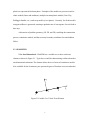


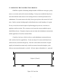
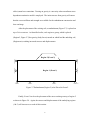

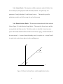
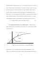
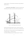


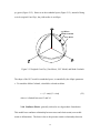


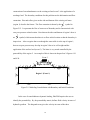


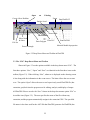

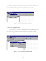
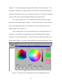


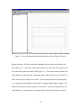

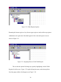
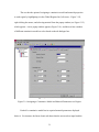
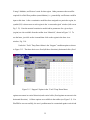
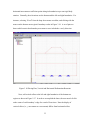


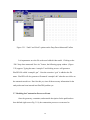

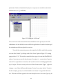
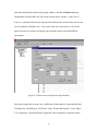

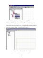


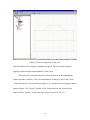
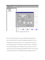
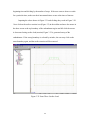
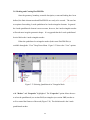

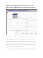
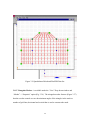
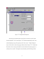
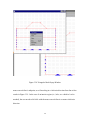
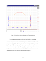

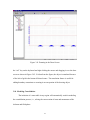
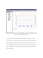


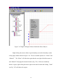
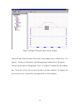
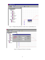


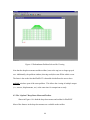

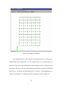
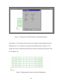


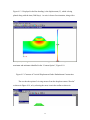
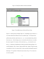
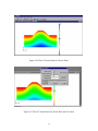


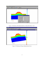

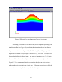
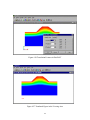
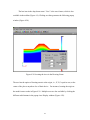
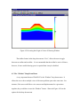

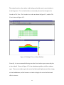


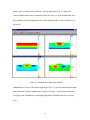
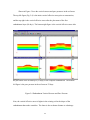
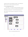
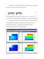


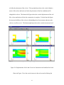
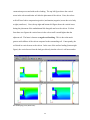

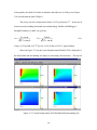
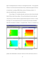


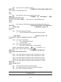


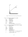


![Comment creuser un tunnel : méthodologie d`excavat[...]](http://vs1.manualzilla.com/store/data/006363996_1-7a025c739c80ffd739a8422978e4c9f6-150x150.png)